discrete element modeling part2. one phase flow
TRANSCRIPT
Numérique avancé – ENSE3 2017
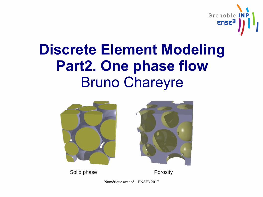
Discrete Element ModelingPart2. One phase flow
Bruno Chareyre

Numérique avancé – ENSE3 2017 p. 2
Content
1. Introduction
2. Fully resolved methods
3. Averaged methods
4. Pore-scale methods
5. Lubrication / dense supsensions
Numérique avancé – ENSE3 2017 p. 3
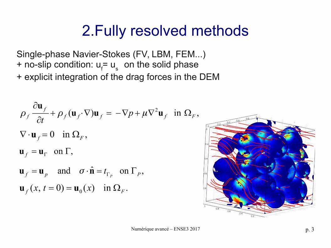
2.Fully resolved methods
Single-phase Navier-Stokes (FV, LBM, FEM...)+ no-slip condition: u
f= u
s on the solid phase
+ explicit integration of the drag forces in the DEM
Numérique avancé – ENSE3 2017 p. 4
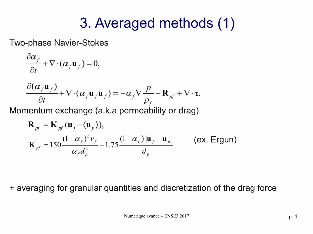
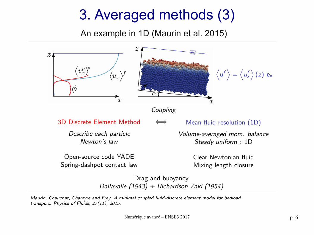
3. Averaged methods (1)Two-phase Navier-Stokes
Momentum exchange (a.k.a permeability or drag)
(ex. Ergun)
+ averaging for granular quantities and discretization of the drag force
Numérique avancé – ENSE3 2017 p. 5
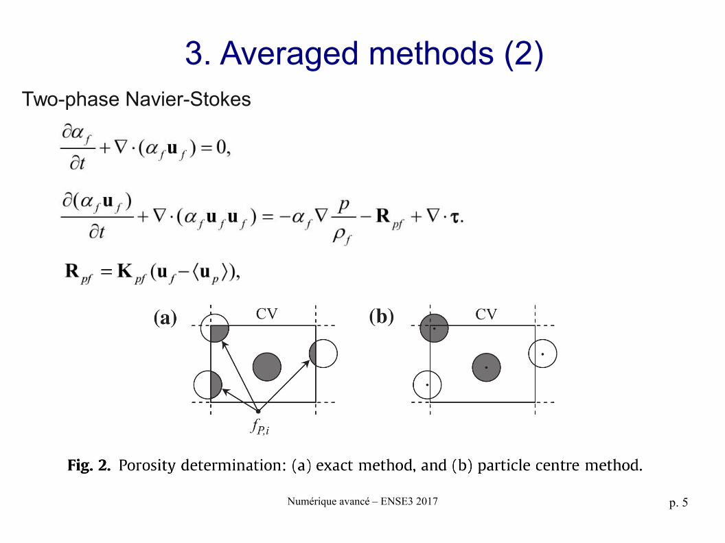
3. Averaged methods (2)Two-phase Navier-Stokes
Numérique avancé – ENSE3 2017 p. 6
3. Averaged methods (3)An example in 1D (Maurin et al. 2015)
Context of this research One fluid phase Two fluid phases (pendular regime) Toward intermediate water contents Conclusions References
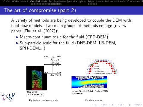
The art of compromise (part 2)
A variety of methods are being developed to couple the DEM withfluid flow models. Two main groups of methods emerge (reviewpaper: Zhu et al. (2007)):
Macro-continuum scale for the fluid (CFD-DEM)
Sub-particle scale for the fluid (DNS-DEM, LB-DEM,SPH-DEM,...)
Equivalent continuum scale Continuum scale
Context of this research One fluid phase Two fluid phases (pendular regime) Toward intermediate water contents Conclusions References
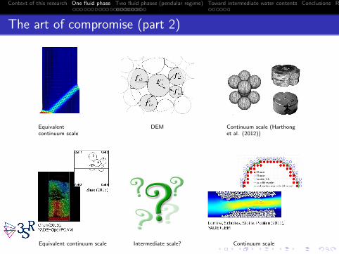
The art of compromise (part 2)
Equivalentcontinuum scale
DEM Continuum scale (Harthonget al. (2012))
Equivalent continuum scale Intermediate scale? Continuum scale
Context of this research One fluid phase Two fluid phases (pendular regime) Toward intermediate water contents Conclusions References
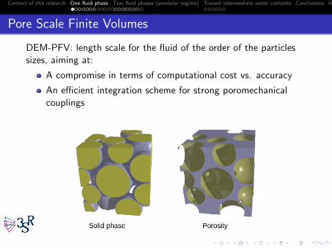
Pore Scale Finite Volumes
DEM-PFV: length scale for the fluid of the order of the particlessizes, aiming at:
A compromise in terms of computational cost vs. accuracy
An efficient integration scheme for strong poromechanicalcouplings
Context of this research One fluid phase Two fluid phases (pendular regime) Toward intermediate water contents Conclusions References
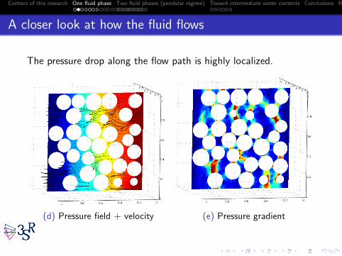
A closer look at how the fluid flows
The pressure drop along the flow path is highly localized.
(d) Pressure field + velocity (e) Pressure gradient
Context of this research One fluid phase Two fluid phases (pendular regime) Toward intermediate water contents Conclusions References
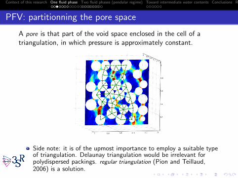
PFV: partitionning the pore space
A pore is that part of the void space enclosed in the cell of atriangulation, in which pressure is approximately constant.
Side note: it is of the upmost importance to employ a suitable typeof triangulation. Delaunay triangulation would be irrelevant forpolydispersed packings. regular triangulation (Pion and Teillaud,2006) is a solution.
Context of this research One fluid phase Two fluid phases (pendular regime) Toward intermediate water contents Conclusions References
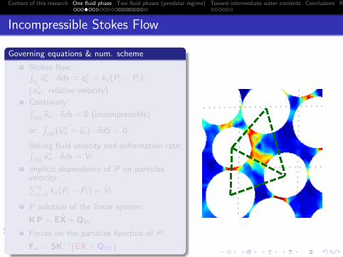
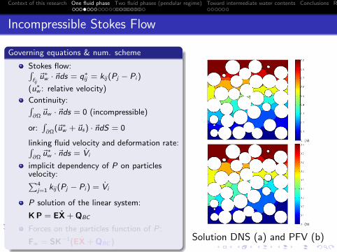
Incompressible Stokes Flow
Governing equations & num. scheme
Stokes flow:∫fij~u∗
w · ~nds = q∗ij = kij (Pj − Pi )
(u∗w : relative velocity)
Continuity:∫∂Ω
~uw · ~nds = 0 (incompressible)
or:∫∂Ω
(~u∗w + ~us ) · ~ndS = 0
linking fluid velocity and deformation rate:∫∂Ω
~u∗w · ~nds = Vi
implicit dependency of P on particlesvelocity:∑4
j=1 kij (Pj − Pi ) = Vi
P solution of the linear system:
KP = EX + QBC
Forces on the particles function of P:
Fw = SK−1(EX + QBC )

Context of this research One fluid phase Two fluid phases (pendular regime) Toward intermediate water contents Conclusions References
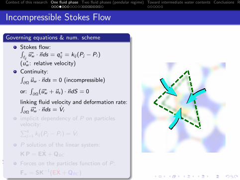
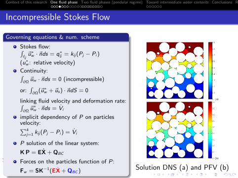
Incompressible Stokes Flow
Governing equations & num. scheme
Stokes flow:∫fij~u∗
w · ~nds = q∗ij = kij (Pj − Pi )
(u∗w : relative velocity)
Continuity:∫∂Ω
~uw · ~nds = 0 (incompressible)
or:∫∂Ω
(~u∗w + ~us ) · ~ndS = 0
linking fluid velocity and deformation rate:∫∂Ω
~u∗w · ~nds = Vi
implicit dependency of P on particlesvelocity:∑4
j=1 kij (Pj − Pi ) = Vi
P solution of the linear system:
KP = EX + QBC
Forces on the particles function of P:
Fw = SK−1(EX + QBC )
Context of this research One fluid phase Two fluid phases (pendular regime) Toward intermediate water contents Conclusions References
Incompressible Stokes Flow
Governing equations & num. scheme
Stokes flow:∫fij~u∗
w · ~nds = q∗ij = kij (Pj − Pi )
(u∗w : relative velocity)
Continuity:∫∂Ω
~uw · ~nds = 0 (incompressible)
or:∫∂Ω
(~u∗w + ~us ) · ~ndS = 0
linking fluid velocity and deformation rate:∫∂Ω
~u∗w · ~nds = Vi
implicit dependency of P on particlesvelocity:∑4
j=1 kij (Pj − Pi ) = Vi
P solution of the linear system:
KP = EX + QBC
Forces on the particles function of P:
Fw = SK−1(EX + QBC ) Solution DNS (a) and PFV (b)
Context of this research One fluid phase Two fluid phases (pendular regime) Toward intermediate water contents Conclusions References
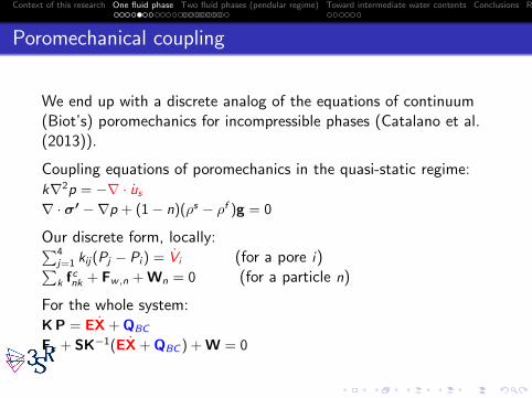
Poromechanical coupling
We end up with a discrete analog of the equations of continuum(Biot’s) poromechanics for incompressible phases (Catalano et al.(2013)).
Coupling equations of poromechanics in the quasi-static regime:k∇2p = −∇ · us
∇ · σ′ −∇p + (1− n)(ρs − ρf )g = 0
Our discrete form, locally:∑4j=1 kij (Pj − Pi ) = Vi (for a pore i)∑k f
cnk + Fw ,n + Wn = 0 (for a particle n)
For the whole system:KP = EX + QBC
Fc + SK−1(EX + QBC ) + W = 0
Context of this research One fluid phase Two fluid phases (pendular regime) Toward intermediate water contents Conclusions References
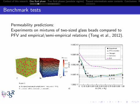
Benchmark tests
Permeability predictions:Experiments on mixtures of two-sized glass beads compared toPFV and empirical/semi-empirical relations (Tong et al., 2012).
Context of this research One fluid phase Two fluid phases (pendular regime) Toward intermediate water contents Conclusions References
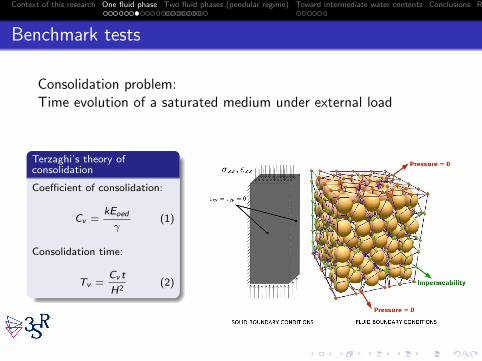
Benchmark tests
Consolidation problem:Time evolution of a saturated medium under external load
Terzaghi’s theory ofconsolidation
Coefficient of consolidation:
Cv =kEoed
γ(1)
Consolidation time:
Tv =Cv t
H2(2)
Context of this research One fluid phase Two fluid phases (pendular regime) Toward intermediate water contents Conclusions References
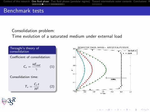
Benchmark tests
Consolidation problem:Time evolution of a saturated medium under external load
Terzaghi’s theory ofconsolidation
Coefficient of consolidation:
Cv =kEoed
γ(1)
Consolidation time:
Tv =Cv t
H2(2)
Context of this research One fluid phase Two fluid phases (pendular regime) Toward intermediate water contents Conclusions References
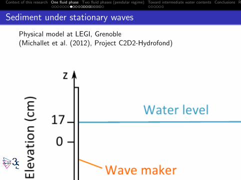
Sediment under stationary waves
Physical model at LEGI, Grenoble(Michallet et al. (2012), Project C2D2-Hydrofond)
(Courtesy of Herve Michallet)

Context of this research One fluid phase Two fluid phases (pendular regime) Toward intermediate water contents Conclusions References
Sediment under stationary waves
Flow regime inside the sediment
Typical values of dimensionless numbers:
Particles Reynolds number: Re ≈ 10−8
Stokes number: Stk →∞ (if relevant)
Mach number: M ≈ 10−8 (numerical model: M = 0)
Steady incompressible viscous flow is a rather good approximation.
Context of this research One fluid phase Two fluid phases (pendular regime) Toward intermediate water contents Conclusions References
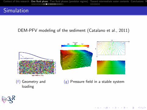
Simulation
DEM-PFV modeling of the sediment (Catalano et al., 2011)
(f) Geometry andloading
(g) Pressure field in a stable system
Context of this research One fluid phase Two fluid phases (pendular regime) Toward intermediate water contents Conclusions References
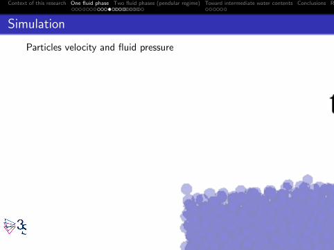
Simulation
Particles velocity and fluid pressure
Context of this research One fluid phase Two fluid phases (pendular regime) Toward intermediate water contents Conclusions References
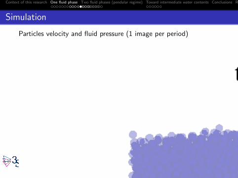
Simulation
Particles velocity and fluid pressure (1 image per period)
Context of this research One fluid phase Two fluid phases (pendular regime) Toward intermediate water contents Conclusions References
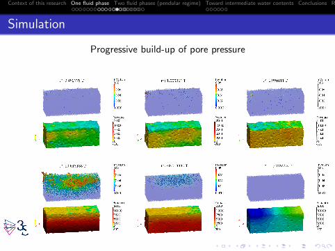
Simulation
Progressive build-up of pore pressure
Context of this research One fluid phase Two fluid phases (pendular regime) Toward intermediate water contents Conclusions References
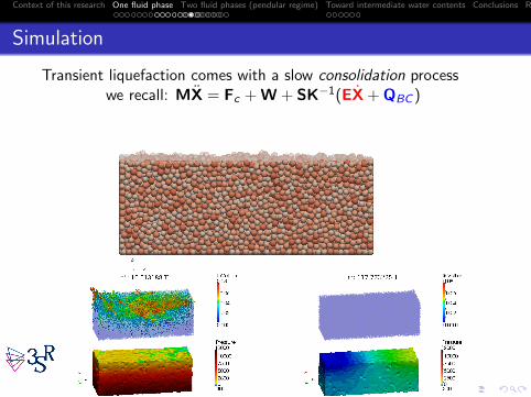
Simulation
Transient liquefaction comes with a slow consolidation processwe recall: MX = Fc + W + SK−1(EX + QBC )

Context of this research One fluid phase Two fluid phases (pendular regime) Toward intermediate water contents Conclusions References
Simulation
Effective stress vanishes (liquefaction)σ′ = 1
Vσ
∑k f
ck ⊗ xk
Context of this research One fluid phase Two fluid phases (pendular regime) Toward intermediate water contents Conclusions References
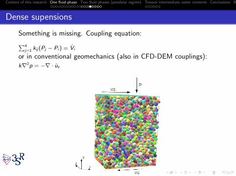
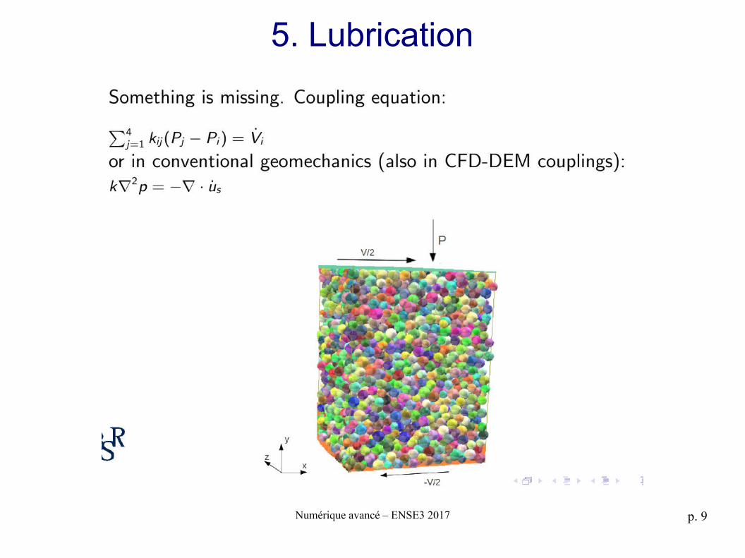
Dense supensions
Something is missing. Coupling equation:∑4j=1 kij (Pj − Pi ) = Vi
or in conventional geomechanics (also in CFD-DEM couplings):k∇2p = −∇ · us
PhD Donia Marzougui (Dir. Chareyre B., Chauchat J.
Context of this research One fluid phase Two fluid phases (pendular regime) Toward intermediate water contents Conclusions References
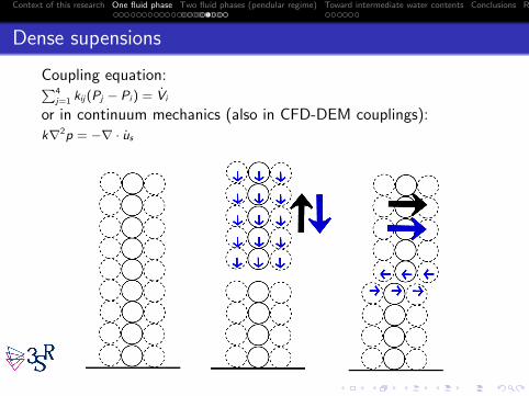
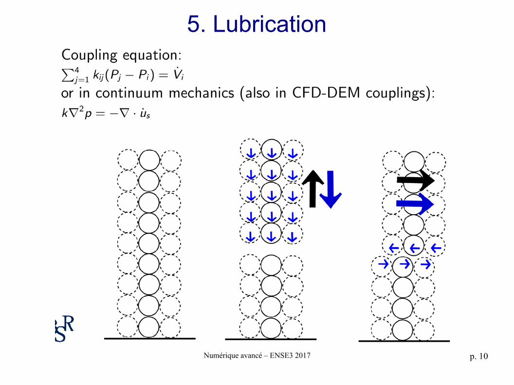
Dense supensions
Coupling equation:∑4j=1 kij (Pj − Pi ) = Vi
or in continuum mechanics (also in CFD-DEM couplings):k∇2p = −∇ · us
Context of this research One fluid phase Two fluid phases (pendular regime) Toward intermediate water contents Conclusions References
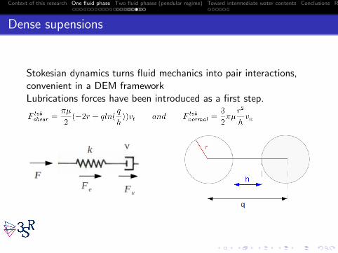
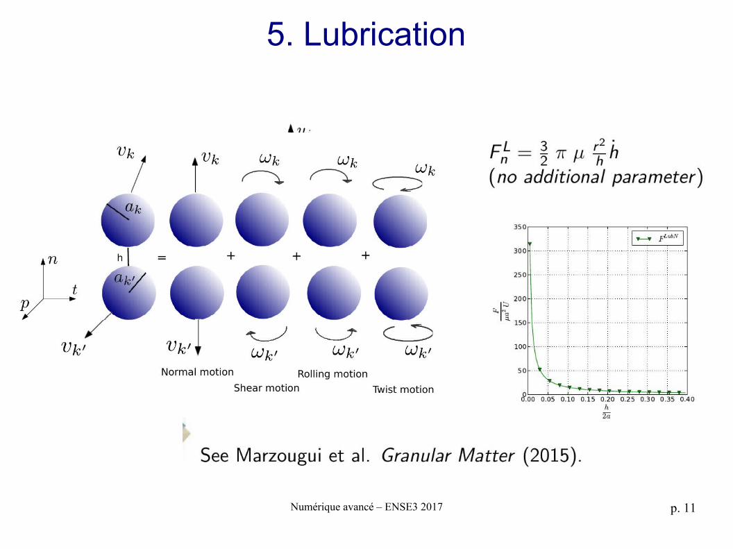
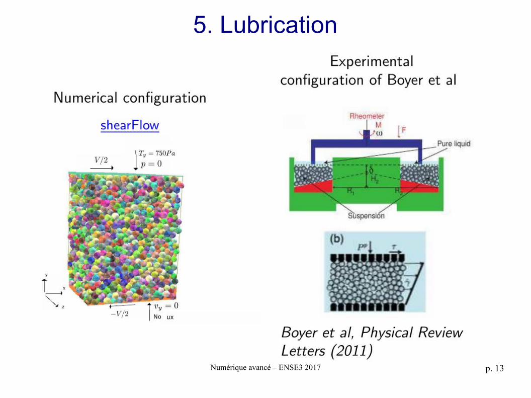
Dense supensions
Stokesian dynamics turns fluid mechanics into pair interactions,convenient in a DEM frameworkLubrications forces have been introduced as a first step.
Numérique avancé – ENSE3 2017 p. 7
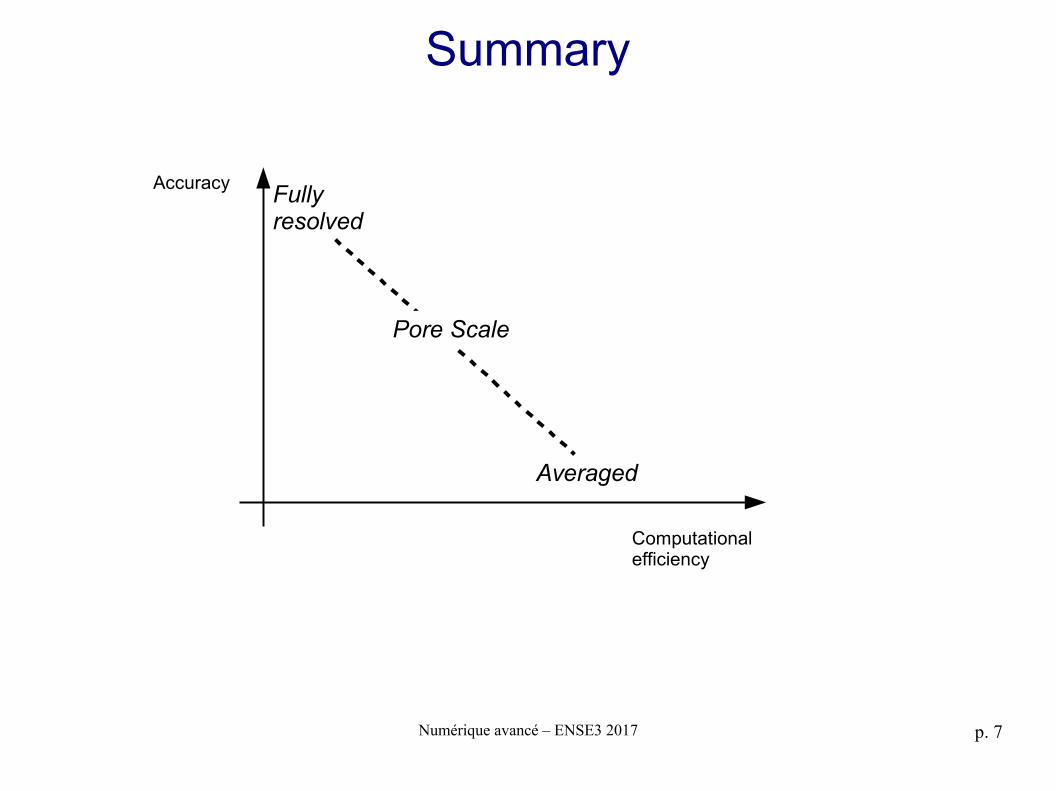
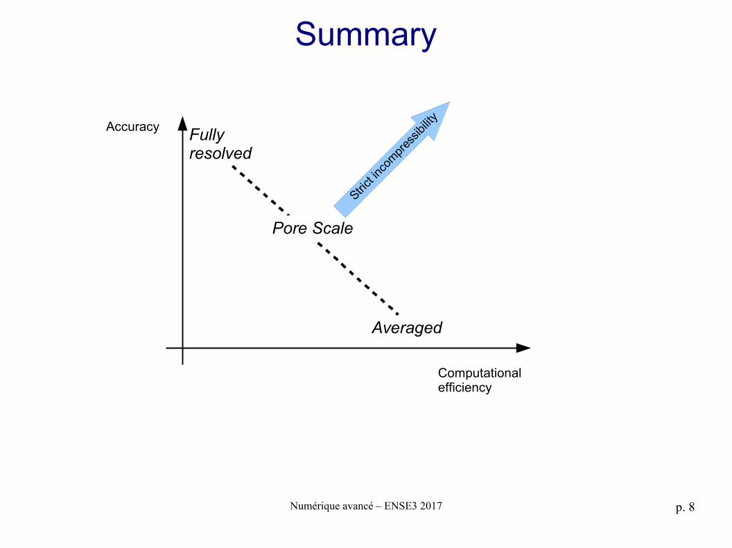
Summary
Computational efficiency
AccuracyFully resolved
Pore Scale
Averaged
Numérique avancé – ENSE3 2017 p. 8
Summary
Computational efficiency
AccuracyFully resolved
Pore Scale
Averaged
Strict
incom
pres
sibilit
y
Numérique avancé – ENSE3 2017 p. 9
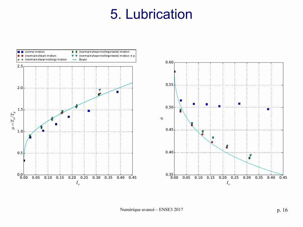
5. Lubrication
Numérique avancé – ENSE3 2017 p. 10
5. Lubrication
Numérique avancé – ENSE3 2017 p. 11
5. Lubrication
Numérique avancé – ENSE3 2017 p. 12
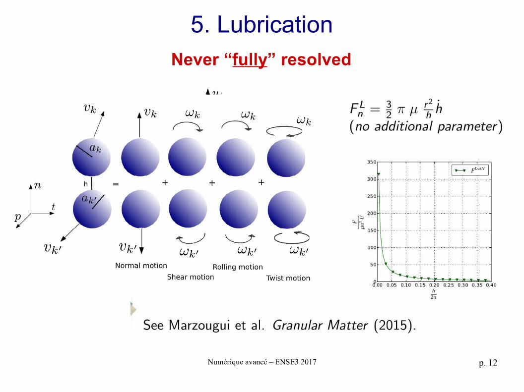
5. LubricationNever “fully” resolved
Numérique avancé – ENSE3 2017 p. 13
5. Lubrication
Numérique avancé – ENSE3 2017 p. 14
5. Lubrication
Numérique avancé – ENSE3 2017 p. 15
5. Lubrication
Numérique avancé – ENSE3 2017 p. 16
5. Lubrication
Numérique avancé – ENSE3 2017 p. 17
Conclusion
- A variety of methods for solving the fluid problem, with three different modeling scales: micro-continuum, pore-scale, macro-continuum (and the corresponding assumptions / computational cost).
- Not all methods handle strict incompressibility efficiently, which may be a problem for strong poro-mechanical coupling.
- None of them will capture the lubrication forces, which dominates the rheology of fluid-grain mixtures. They need to be introduced in addition to the resolved drag forces (possibly with some cut-off).