discrete event simulation prof nelson fonseca state university of campinas, brazil
Post on 22-Dec-2015
213 views
TRANSCRIPT

Discrete Event Simulation
Prof Nelson FonsecaState University of Campinas,
Brazil
Simulation
• Emulation – hardware/firmware simulation
• Monte-carlo simulation – static simulation, typically for evaluation of numerical expressions
• Discrete event simulation – dynamic system, synthetic load
• Trace driven simulation – dynamic systems, traces of real data as input

Networks & Queues

Queuing
Telephone
Computer
Computer

Measures of Interest
• Waiting time in the queue
• Waiting time in the system
• Queue length distribution
• Server utilization
• Overflow probability

Discrete Event Simulation
• Represents the stochastic nature of the system being modeled
• Driven by the occurrence of events
• Statistical experiment

Discrete Event Simulation

Events
• State Variables – Define the state of the system– Example: length of the queue
• Event: change in the system– Examples: arrival of a client,
departure of a client

Discrete Events
• Occurance of event – needs to reflect the changes in the system due to the occurance of that event
Discrete Events
• Primary event – an event which occurrence is scheduled at a certain time
• Conditional event an event triggered by a certain condition becoming true

Discrete Event Simulation
• The future event list (FEL) …– Controls the simulation– Contains all future events that are
scheduled– Is ordered by increasing time of event
notice– Contains only primary events
• Example FEL for some simulation time t≤T1:(t1, Event1) (t2, Event2) (t3, Event3) (t4, Event4)
t1≤ t2≤ t3≤ t4
Discrete Event Simulation
• Operations on the FEL:– Insert an event into FEL (at appropriate
position)– Remove first event from FEL for processing– Delete an event from the FEL
• The FEL is thus usually stored as a linked list
• The simulator spends a lot of time processing the FEL– Efficiency is thus very important!

DES
FELempty?
yes
noRemove and process first primary event
Conditionalevent enabled? noyes
Process conditional event
DES
• Simulation clock register virtual time, not real time
• Can simulate one century in a second

DESSimulation clock: t2
(t2, Arrival) (t3, Service complete)

Book Keeping
• Procedures that collect information (logs) about the dynamics of the simulated system to generate reports
• Can collect information at the occurance of every event or every fixed number of events

Simulating a Queue
Simulation clock:
Arrival Customer Begin Service Serviceinterval arrives service duration complete
5 5 5 2 71 6 7 4 113 9 11 3 143 12 14 1 15
15

Computing Statistics
Average waiting time for a customer: (0+1+2+2)/4=1.25
Arrival Customer Begin Service Serviceinterval arrives service duration complete
5 5 0 5 2 71 6 1 7 4 113 9 2 11 3 143 12 2 14 1 15

Computing Statistics
P(customer has to wait): =3/4=0.75
Arrival Customer Begin Service Serviceinterval arrives service duration complete
5 5 5 2 71 6 W 7 4 113 9 W 11 3 143 12 W 14 1 15
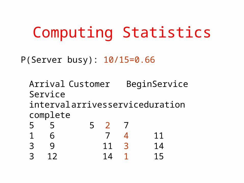
Computing Statistics
P(Server busy): 10/15=0.66
Arrival Customer Begin Service Serviceinterval arrives service duration complete
5 5 5 2 71 6 7 4 113 9 11 3 143 12 14 1 15

Computing Statistics
Average queue length: =(1*1+2*1+2*1)/15=0.33
Arrival Customer Begin Service Serviceinterval arrives service duration complete
5 5 0 5 2 71 0 6 1 7 4 113 0 9 1 11 3 143 0 12 1 14 1 0 15
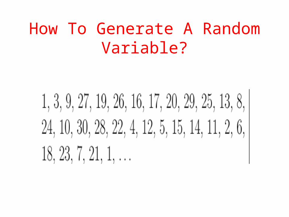
How To Generate A Random Variable?

How To Generate A Random Variable?

How To Generate A Random Variable?
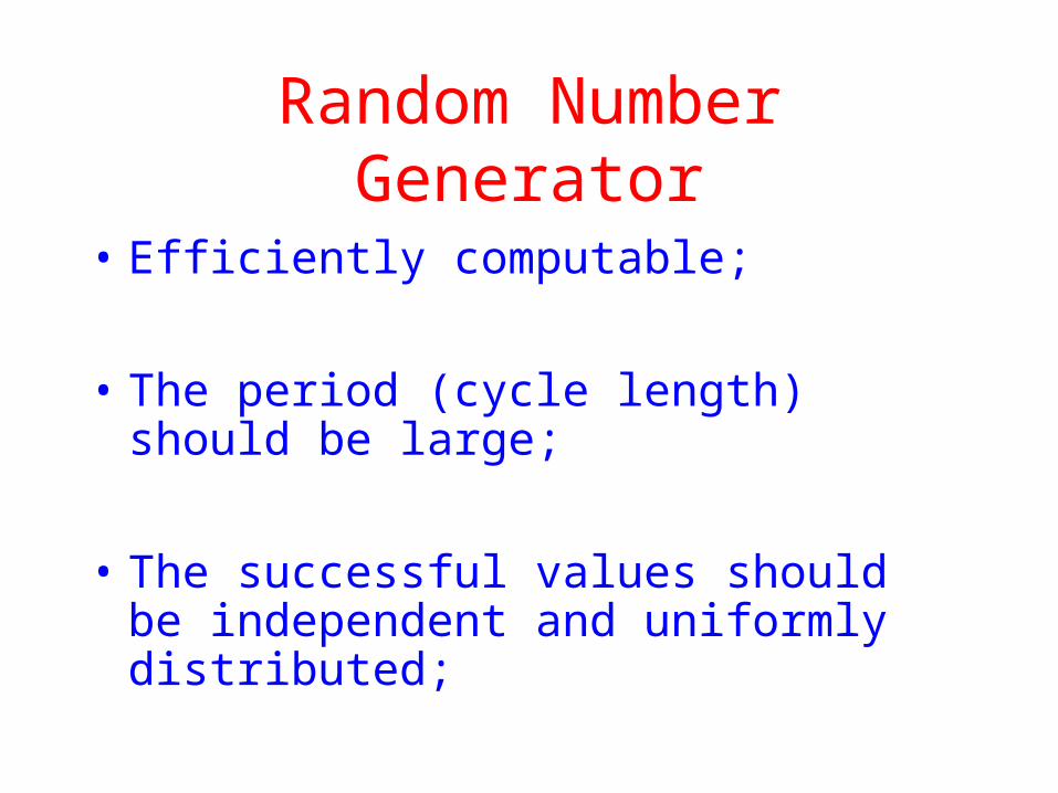
Random Number Generator
• Efficiently computable;
• The period (cycle length) should be large;
• The successful values should be independent and uniformly distributed;

How To Generate A Random Variable?
• Linear congruential method
• Xn+1 = (a Xn + b) modulo m
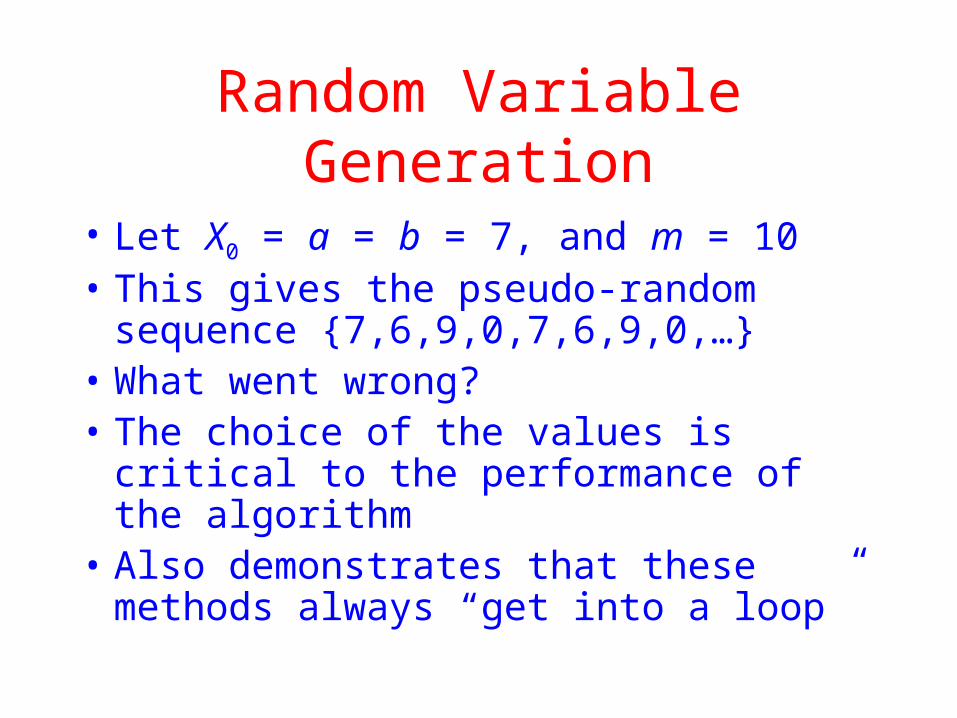
Random Variable Generation
• Let X0 = a = b = 7, and m = 10• This gives the pseudo-random
sequence {7,6,9,0,7,6,9,0,…}• What went wrong?• The choice of the values is critical
to the performance of the algorithm• Also demonstrates that these
methods always “get into a loop”

Linear Congruential Method
• a, b and m affect the period and autocorrelation
• Value depend on the size of memory word
• The modulus m should be large – the period can never be more than m
• For efficiency m should be power of 2– mod m can be obtained by truncation

Linear Congruential Method
• If b is non-zero, the maximum possible period m is obtained if and only if:
– m and b are relatively prime, i.e., has non common factor rather than 1
– Every prime number that is a factor of m should be a factor of a-1

Linear Congruential Method
• If m is a multiple of 4, a-1 should be a multiple of 4;
• All conditions are met if: – m = 2k, a = 4c + 1– c, b and k are positive integer

Multiplicative Congruential Method
• b=0 period reduced, faster
Xn = a Xn-1 modulo m
• m = 2k – maximum period 2k-2
• m prime number – with proper multiplier a maximum period m-1

Unix
• m= 248
• a = 0x5DEECE66D
• b = 0xB
• errand48(), lrand48(), nrand48(), mrand48(), jrand48()

Period

Seeds
• Initial value – right choice to maximize period length
• Depends on a, b and m

Seeds

Multiple Streams of Random Number
• Avoid correlation of events• Single queue: Different streams for
arrival and service time• Multiple queues: multiple streams• Do not subdivide a stream• Do not generate successive seeds
to initially feed multiple streams
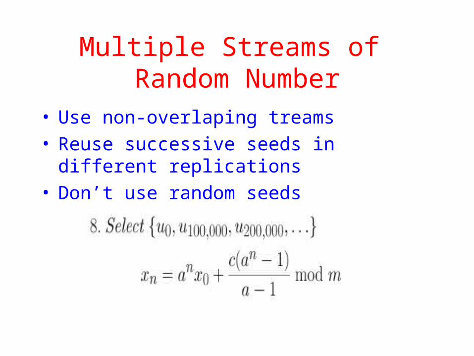
Multiple Streams of Random Number
• Use non-overlaping treams• Reuse successive seeds in different
replications• Don’t use random seeds
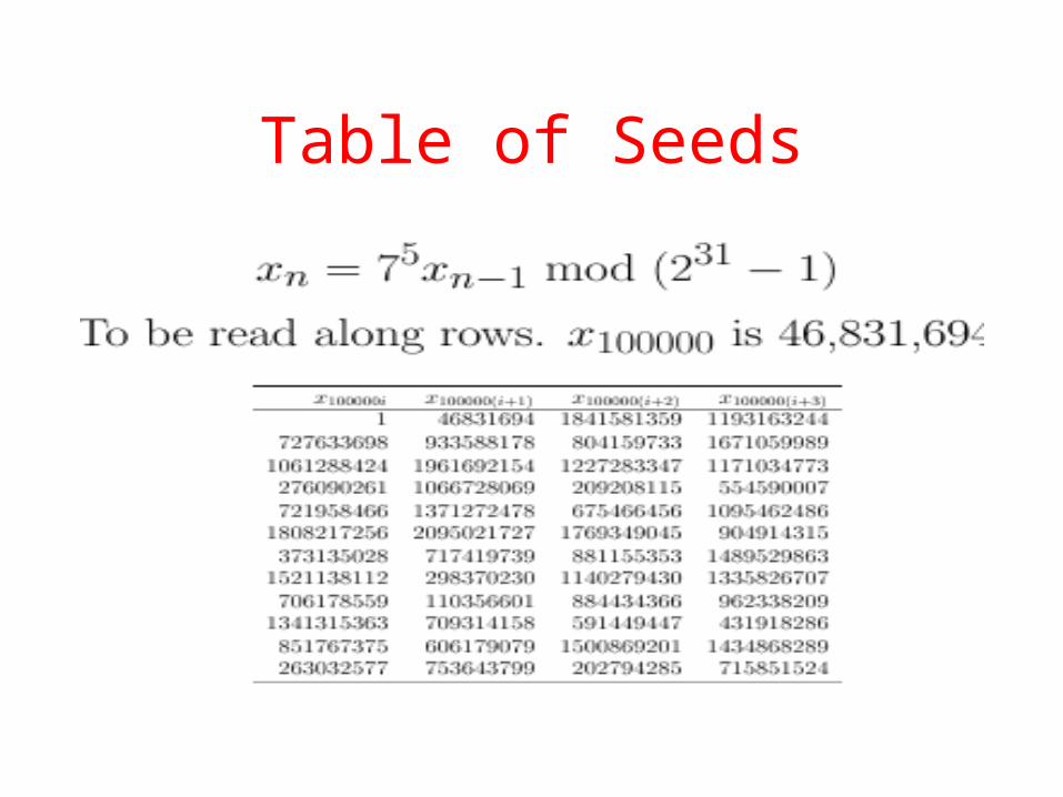
Table of Seeds

Random Number Generators
• Tausworthe Generator
• Extended Fibonacci Generator
• Combined generator

Random Variate Generation
• We have a sequence of pseudo-random uniform variates. How do we generate variates from different distributions?
• Random behavior can be programmed so that the random variables appear to have been drawn from a particular probability distribution
• If f(x) is the desired pdf, then consider the CDF
• This is non-decreasing and lies between 0 and 1
x
x dxxfxF )()(
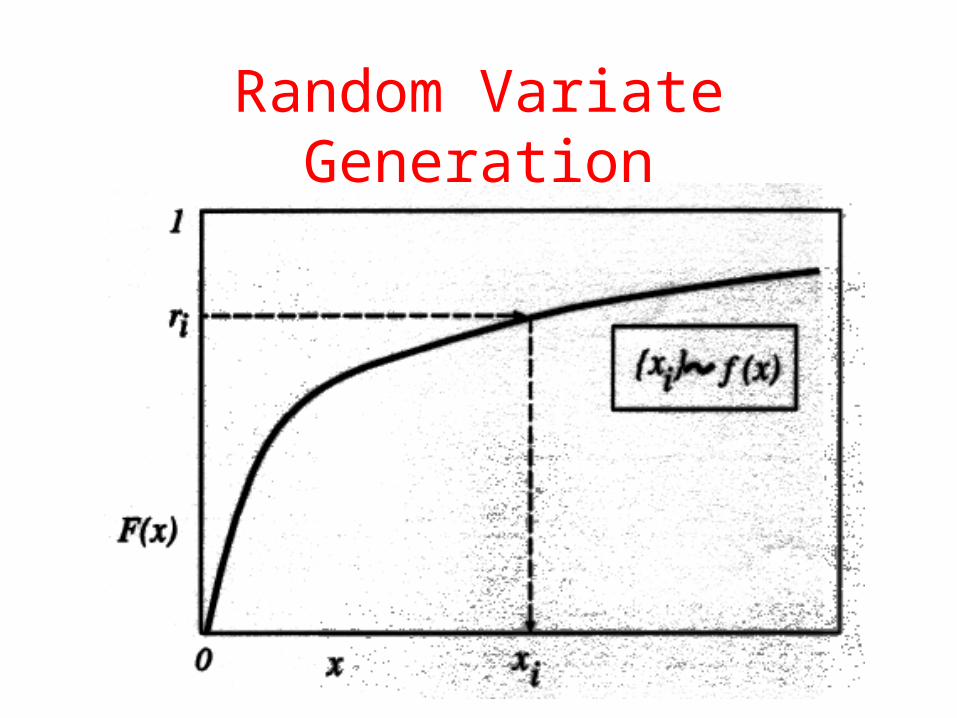
Random Variate Generation
• Given a sequence of random numbers ri distributed over the same range (0,1)
• Let each value of ri be a value of the function Fx(x)
• Then the corresponding value xi is uniquely determined
• The sequence xi is randomly distributed and has the probability density function f(x)
Random Variate Generation

Random Variate Generation

Method of Inverse
• For the exponential distribution
• For positive xi
• Thus
ixix exF 1)(
)1ln(1
)1ln(
1
1
ii
ii
xi
xi
rx
xr
er
eri
i
Method of Inverse
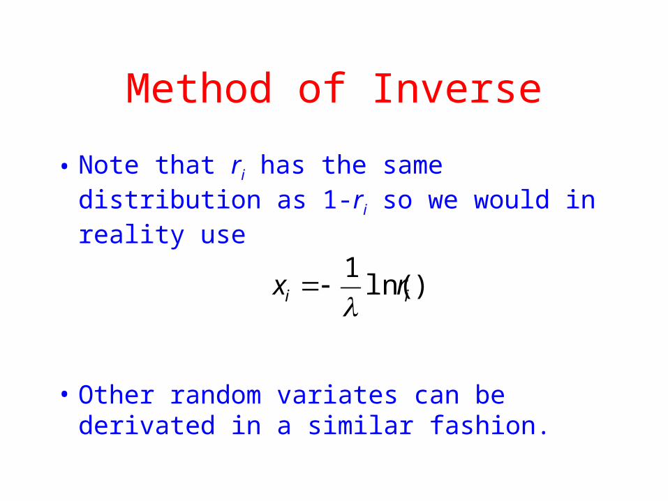
• Note that ri has the same distribution as 1-ri so we would in reality use
• Other random variates can be derivated in a similar fashion.
)ln(1
ii rx
Method of Inverse

Method of Inverse

Rejection-acceptance

Rejection-acceptance

Rejection-acceptance

Composition

Composition

Convolution
• Random variable is given by the sun of independent random variable
• Examples: erlang, binomial, chi-square

Convolution
• Example: Erlang random variable is the sum of independent exponentially distributed random variables
Step1: Generate U1, U2, …Uk independent and uniformly distributed between 0 and 1
Step2: Compute X= –-1 ln(U1 U2…Uk)
)!1/()( 1 kxexf kkxx

Convolution

Characterization
• Algorithm tailored to the variate by drawing from transformation, etc
• Example: Poisson can be generated by continuosly generating exponential distribution until exceeds a certain value
Characterization
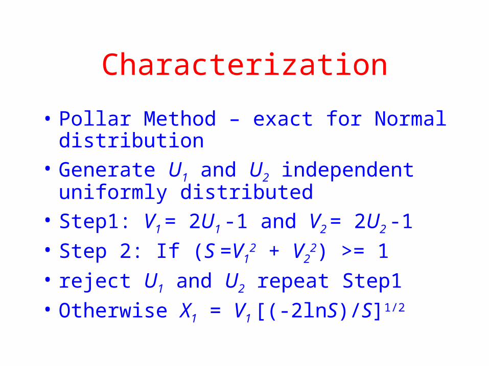
• Pollar Method – exact for Normal distribution
• Generate U1 and U2 independent uniformly distributed
• Step1: V1 = 2U1 -1 and V2 = 2U2 -1• Step 2: If (S =V1
2 + V22) >= 1
• reject U1 and U2 repeat Step1• Otherwise X1 = V1 [(-2lnS)/S]1/2

Random Variate Generation

Random Variate Generation

Steady State Distribution

Transient Removal
• Identifying the end of transient state• Long runs• Proper initialization• Truncations• Initial data collection• Moving average of independent
replication• Batch means
Transient RemovalLong Runs
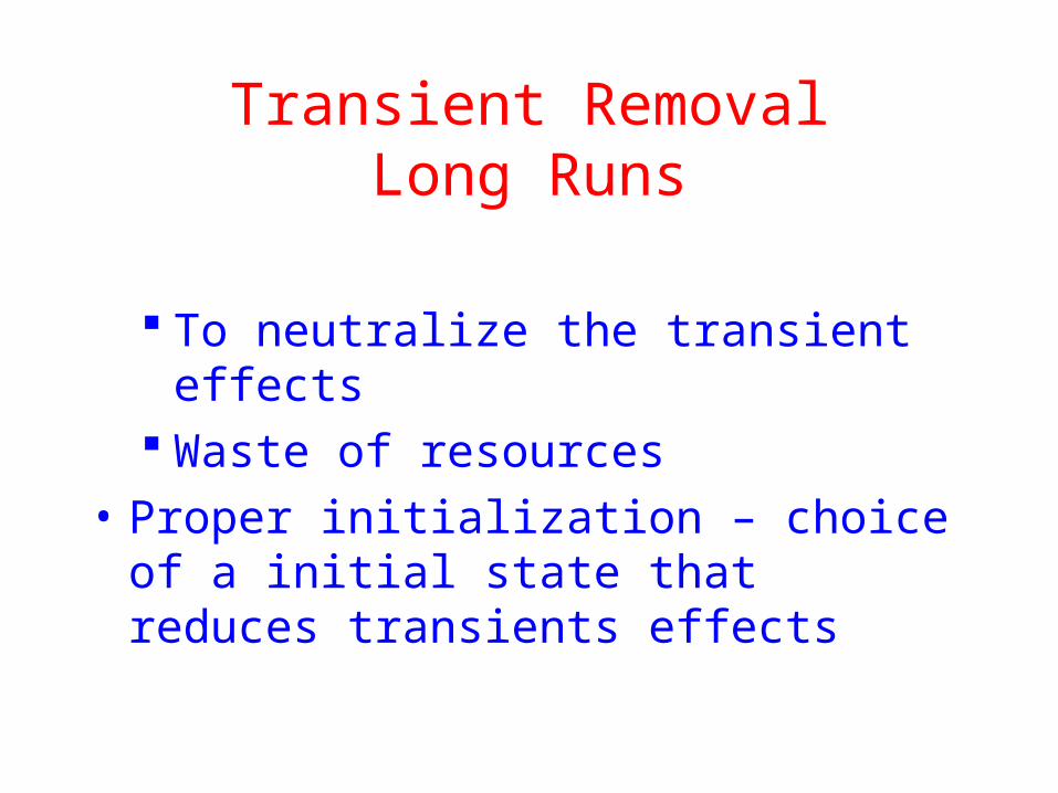
To neutralize the transient effects
Waste of resources• Proper initialization – choice of a
initial state that reduces transients effects

Transient RemovalTruncation
• Low variability in steady state• Plots max-min n – j (j = 1, 2..)
observations• When (j+1)th observation is neither
the minimum nor the maximum – transient ended
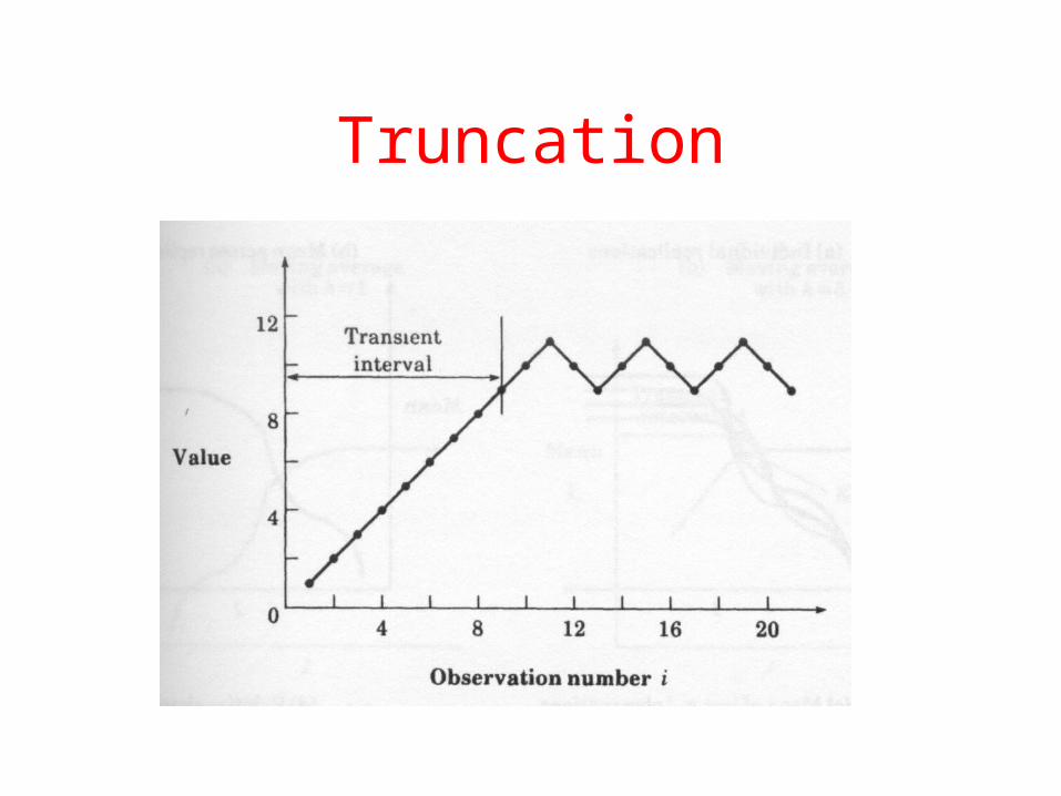
Truncation

Transient RemovalDeletion of Initial
Observation
• No change on average value – steady state
• Produce several replications• Compute the mean• Delete j observation and check whether
the sample mean was achieved. When found such j the duration of transient is determined

Transient RemovalDeletion of Initial
Observation

Transient Removal Moving average
independent replication
• Similar to initial deletion method but the mean is computed over moving time interval instead of overall mean

Transient Removal Moving average
independent replication

Transient RemovalBatch Mean
• Take a long simulation run• Divide the observation into intervals• Compute the mean of this intervals• Try different sizes of batches• When variance of batch mean starts
to decrease – found the size of transient

Transient RemovalBatch Mean

Simulation: A Statistical Experiment
Simulation: A Statistical Experiment
• “Any estimate will be a random variable. Consequently a fixed, deterministic quantity must be estimated by a random quantity”
• “The experimenter must generate from the simulation not only an estimate but also enough information about the probability distribution so that reasonable confidence on the unknown value can be achieved”

Statistical Analysis of Results
• Given that each independent replication of a simulation experiment will yield a different outcome…
• To make a statement the about accuracy we have to estimate the distribution of the estimator
• Need to determine that the distribution becomes asymptotically centered around the true value

Statistical Analysis of Results
• Cannot be established with certainty in the case of a finite simulation
• The usual method used to estimate variability is to produce “confidence interval” estimates

Confidence Interval
Confidence Intervals
• Given some point estimate p a we produce a confidence interval (p-, p+)
• The “true” value is estimated to be contained within the interval with some chosen probability, e.g. 0.9
• The value depends on the confidence level – the greater the confidence, the larger the value of

The central circle has a radiu of 20 cm, only 5% of the arrows are thrown out of the circle
An observer does not know where the circle is centered
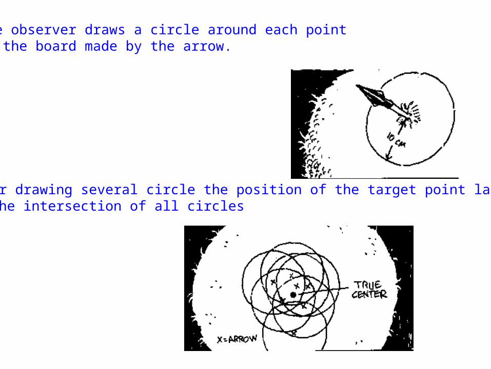
The observer draws a circle around each point on the board made by the arrow.
After drawing several circle the position of the target point laysIn the intersection of all circles
Confidence Intervals
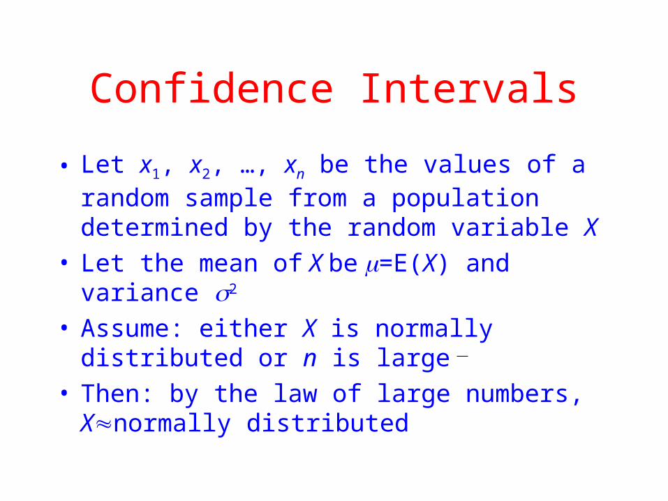
• Let x1, x2, …, xn be the values of a random sample from a population determined by the random variable X
• Let the mean of X be =E(X) and variance 2
• Assume: either X is normally distributed or n is large
• Then: by the law of large numbers, Xnormally distributed

Central Limit Theorem
• The sum of a large number of independent observations from any distribution tends to have a normal distribution:
)/,(~ nNx
Standard deviation

Central Limit Theorem

Confidence Intervals
• Then, given the 100(1-)% confidence interval is given by
where(2)
• z is defined to be the largest value of z such that P(Z>z)= and Z is the standard normal random variable
x
n
z 2/

Confidence Interval
nszxnszx /,/ 2/12/1
Confidence Intervals
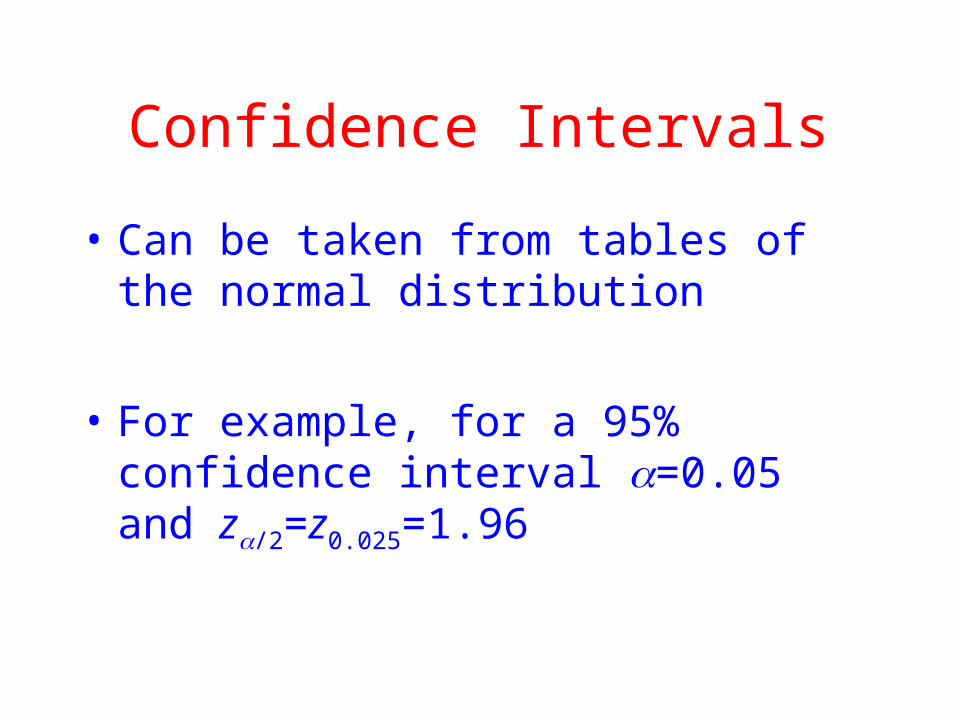
• Can be taken from tables of the normal distribution
• For example, for a 95% confidence interval =0.05 and z/2=z0.025=1.96

Confidence level = 95%, = 0.05 and p = 1 – /2

Example
• = 3,90; s=0,95 e n=32.
• Confidence level of 90%
• Confidence level of 95%
• Confidence level of 99%
)17,4;62,3(32/)95,0)(645,1(90,3
)23,4;57,3(32/)95,0)(960,1(90,3
)33,4;46,3(32/)95,0)(576,2(90,3
x

Using Student`s T
• When we know neither nor we can use the observed sample mean x and sample standard deviation s
• If n is large then we simply use s for in Equation (2).
• If n is small and X is normally distributed then we may use
n
t s2/

Using Student`s T• The ratio for samples from normal
populations follows a t (n-1) distribution
• t/2 is defined by P(T>t/2)=/2
• T has a Student-t distribution with n-1 degrees of freedom
• This is the more frequently used formula in simulation models
nS
x

t Student
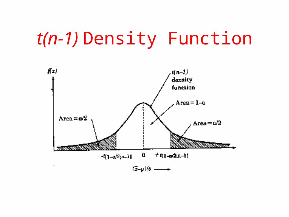
t(n-1) Density Function

Confidence Interval
1}/)2/1(ˆ/)2/1(ˆ{Prob
/
ˆ
)(11
1)(
1
1ˆ
1ˆ
2/11
2/11
2/1
2
1
2
1
222
1
MstMst
Ms
XM
MX
MXX
Ms
XM
X
MM
M
mm
M
mm
M
mm

Confidence Interval

Confidence IntervalVariance Estimation
M
jmm
XMj
X
XM
MM
jmm
XMj
1
1
2)(2
122
12̂
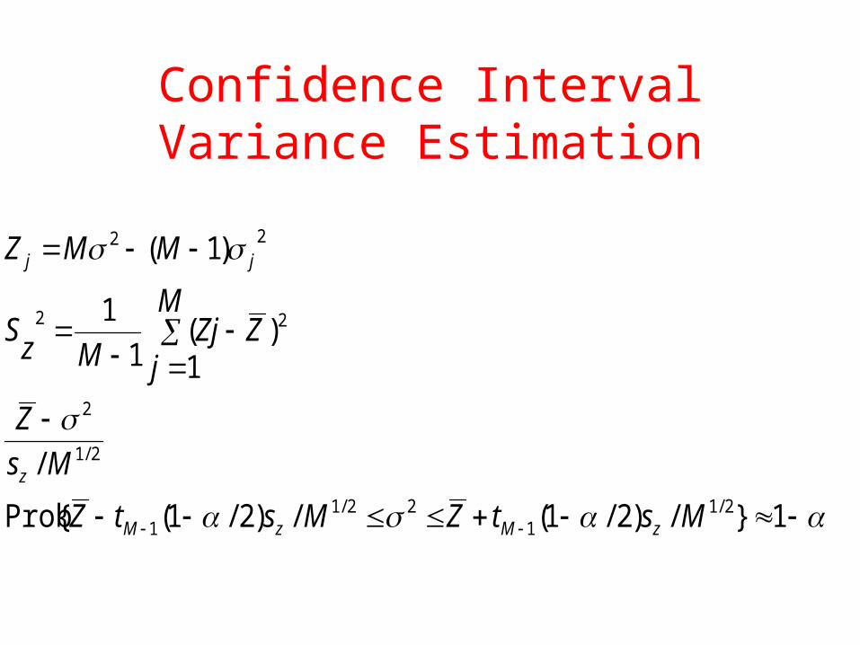
Confidence IntervalVariance Estimation
1}/)2/1(/)2/1({Prob
/
1)(
1
1
)1(
2/11
22/11
2/1
2
22
22
MstZMstZ
Ms
Z
M
jZZj
MzS
MMZ
zMzM
z
jj

Independent Replications
• Generate several sample paths for the model which are statistically independent and identically distributed.
• Reset the model performance measures at the beginning of each replication,
• Use a different random number seed for each independent replication

Independent Replications
• Distributions of the performance measures can then be assumed to have finite mean and variance
• With sufficient replications the average over the replications can be assumed to have a Normal distribution
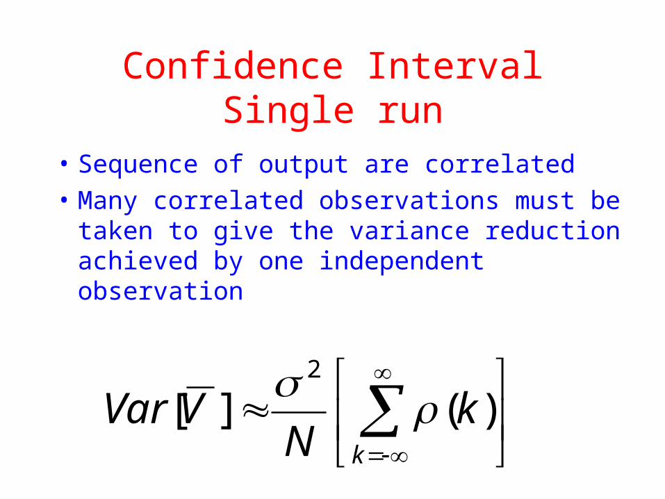
Confidence IntervalSingle run
• Sequence of output are correlated• Many correlated observations must be
taken to give the variance reduction achieved by one independent observation
k
kN
VVar )(][2
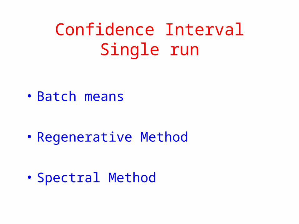
Confidence IntervalSingle run
• Batch means
• Regenerative Method
• Spectral Method
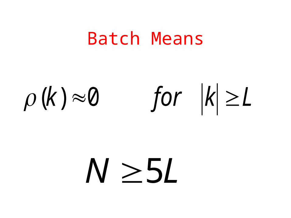
Batch Means
Lkfork 0)(
LN 5

Batch Means
• Divide data in batches (sub-sample) and compute the mean of each batch
• The confidence interval is computed in the same way as in the independent replication method, except that samples are the batch means instead of means from different replications
• Discard lower amount of data than the replication method

Batch Means

Batch Means
Regenerative Method
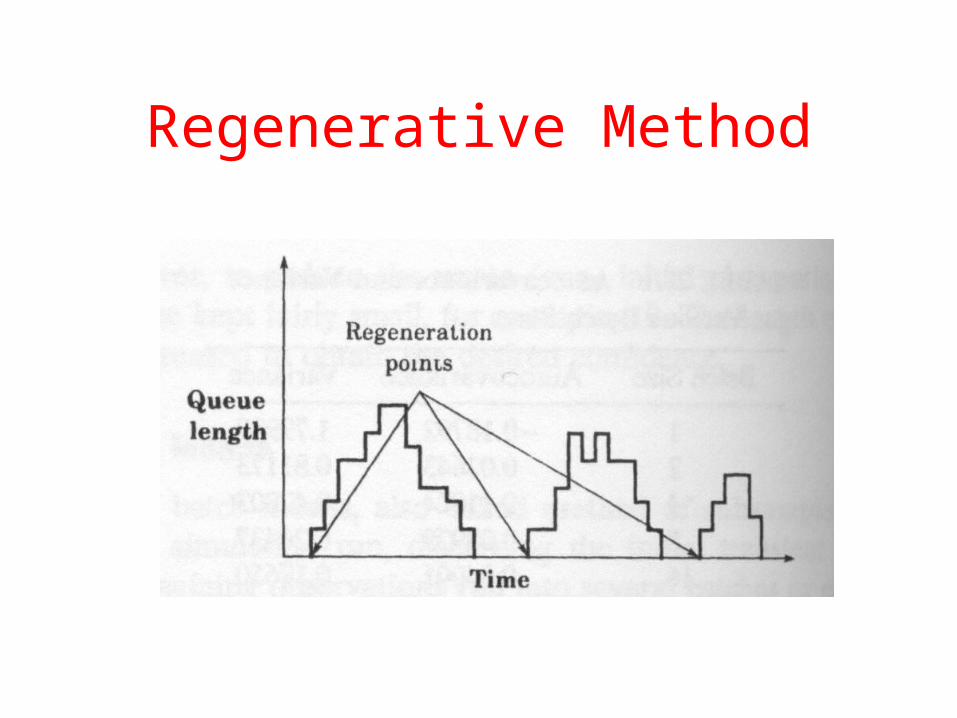
• Points of regeneration – no memory
• Tour - each period of regeneration
• Compute the desired value by taking the mean of the values obtained in each tour
Regenerative Method
Spectral Method
• Compute the correlation between runs
• Does not assume independent runs
• Confidence interval takes into account correlation between runs
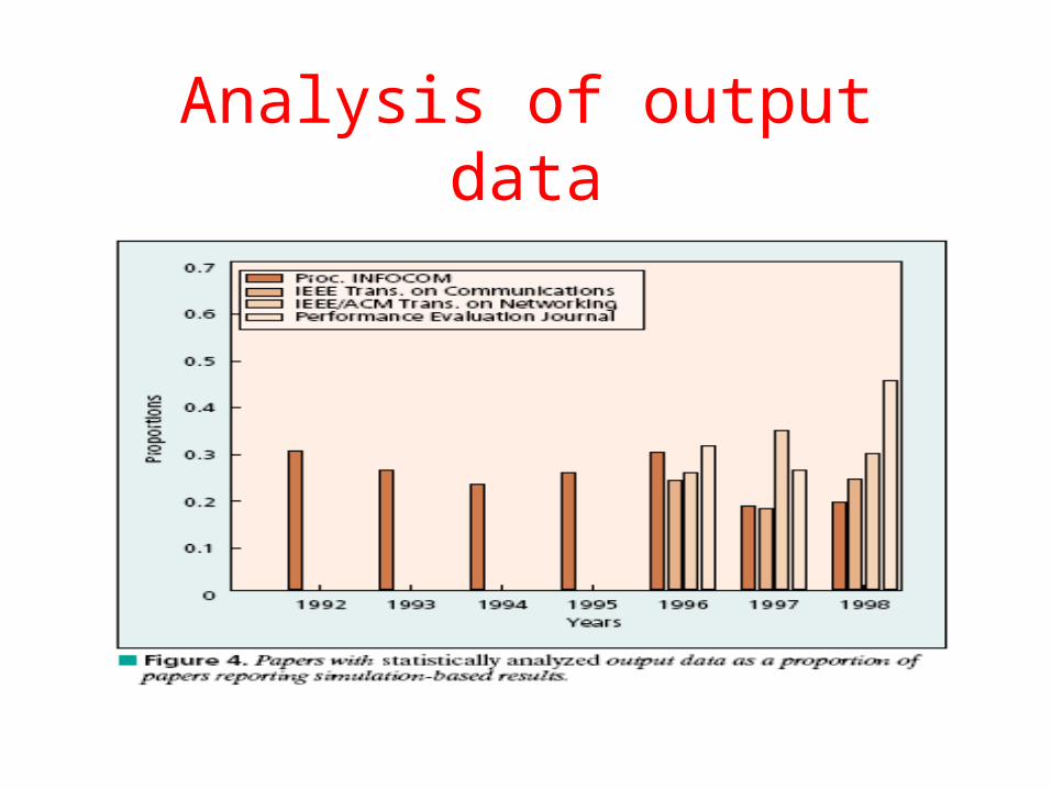
Analysis of output data

Trace Driven Simulation
• Trace – time ordered record of events on a system
– Example : sequence of packets transmitted in a link
• Trace-driven simulation – trace input
Trace Driven Simulation
• Easy validation
• Accurate workload
• Less randomness
• Allow better understanding of complexity of real system

Trace Driven Simulation
• Representativiness
• Finiteness (huge amount of data)
• Difficult to collect data
• Difficult to change input parameters
Multiprocessed Simulation
• Work on a single simulation run
• Distributed Simulation
• Parallel Simulation

References
• Stephen Lavenberg, Computer Performance Modeling Handbook, Academic Press, 1983
• Raj Jain, “The art of Computer Systems Performance Analysis”, John Wiley and Sons, 1991