Discrete optimization methods to fitpiecewise-affine models to data points

E. Amaldi+, S. Coniglio∗?, L. Taccari+

+Dipartimento di Elettronica, Informazione e Bioingegneria,Politecnico di Milano

Piazza Leonardo da Vinci 32, 20133 Milano, Italy∗Lehrstuhl II fur Mathematik

RWTH Aachen UniversityPontdriesch 14-16, 52062 Aachen, Germany

edoardo.amaldi@polimi.it, coniglio@math2.rwth-aachen.de,

leonardo.taccari@polimi.it

Abstract. Fitting piecewise affine models to data points is a perva-sive task in many scientific disciplines. In this work, we address the k-Piecewise Affine Model Fitting with Pairwise Linear Separability problem(k-PAMF-PLS) where, given a set of m points {a1, . . . ,am} ⊂ Rn andthe corresponding observations {b1, . . . , bm} ⊂ R, we have to partitionthe domain Rn into k pairwise linearly separable subdomains and to de-termine an affine submodel (function) for each of them so as to minimizethe total linear fitting error w.r.t. the observations bi.

To solve k-PAMF-PLS to optimality, we propose a mixed-integer linearprogramming (MILP) formulation where symmetries are broken by sep-arating the so-called shifted column inequalities. For medium-to-largescale instances, we develop a four-step heuristic involving, among others,a point reassignment step based on the identification of critical pointsand a domain partition step based on multicategory linear classifica-tion. Differently from traditional approaches proposed in the literaturefor similar fitting problems, in our methods the domain partitioning andsubmodel fitting aspects are taken into account simultaneously.

Computational experiments on real-world and structured randomly gen-erated instances show that, with our MILP formulation with symmetrybreaking constraints, we can solve to proven optimality many small-sizeinstances. Our four-step heuristic turns out to provide close-to-optimalsolutions for small-size instances, while allowing to tackle instances ofmuch larger size. The experiments also show that the combined impactof the main features of our heuristic is quite substantial when comparedto standard variants not including them.

? The work of S. Coniglio was carried out, for a large part, while he was with Di-partimento di Elettronica, Informazione e Bioingegneria, Politecnico di Milano. Thepart carried out while with Lehrstuhl II fur Mathematik, RWTH Aachen University,is supported by the German Federal Ministry of Education and Research (BMBF),grant 05M13PAA, and Federal Ministry for Economic Affairs and Energy (BMWi),grant 03ET7528B.

1 Introduction

Fitting a set of data points in Rn with a combination of low complexity mod-els is a pervasive problem in, essentially, any area of science and engineering.It naturally arises, for instance, in prediction and forecasting when determin-ing a model to approximate the value of an unknown function, or wheneverone wishes to approximate a highly complex nonlinear function with a simplerone. Applications range from optimization (see, e.g., [TV12] and the referencestherein) to data mining (see, e.g., [AM02]) and system identification (see, forinstance, [BGPV03,FTMLM03,TPSM06]), only to cite a few.

Among the different options, piecewise affine models have a number of advan-tages with respect to other model fitting approaches. Indeed, they are compactand simple to evaluate, visualize, and interpret, in contrast to models obtainedwith other techniques such as, e.g., neural networks, while allowing to approxi-mate even highly nonlinear functions.

Given a set of m points A = {a1, . . . ,am} ⊂ Rn, where I = {1, . . . ,m}, withthe corresponding observations {b1, . . . , bm} ⊂ R and a positive integer k, thegeneral problem of fitting a piecewise affine model to the data points {(a1, b1), . . . , (am, bm)}consists in partitioning the sub-domain Rn into k continuous subdomainsD1, . . . , Dk,where J = {1, . . . , k}, and in determining, for each subdomain Dj , an affinesubmodel (an affine function) fj : Dj → R, so as to minimize a measure of

the total fitting error. Adopting the notation fj(x) = wjx − wj0 with coeffi-

cients (wj , wj0) ∈ Rn+1, the j-th affine submodel corresponds to the hyperplane

Hj = {(x, fj(x)) ∈ Rn+1 : fj(x) = wjx−wj0} where x ∈ Dj . The total fitting er-

ror is defined as the sum, over all i ∈ I, of a function of the difference between biand the value fj(i)(ai) provided by the piecewise affine model, where j(i) isthe index of the affine submodel corresponding to the subdomain Dj(i) whichcontains the point ai.

In the literature, different error functions (e.g., linear or quadratic) as wellas different types of domain partition (with linearly or nonlinearly separablesubdomains) have been considered. See Figure 1 (a) for an illustration of thecase with k = 2 and a domain partition with linearly separable subdomains.

In this work, the focus is on the version of the general piecewise affine modelfitting problem with a linear error function (L1 norm) and a domain partitionwith pairwise linearly separable subdomains. We refer to it as to the k-PiecewiseAffine Model Fitting with Pairwise Linear Separability problem (k-PAMF-PLS).A more formal definition of the problem will be provided in Section 3.

k-PAMF-PLS shares a connection with the so-called k-Hyperplane Cluster-ing problem (k-HC), an extension of a classical clustering problem which callsfor k hyperplanes in Rn+1 that minimize the sum, over all the data points{(a1, b1), . . . , (am, bm)}, of the L2 distance from (ai, bi) to the hyperplane it isassigned to. See [BM00,AC13,Con11,Con15] for some recent work on the prob-lem and [ADC13] for the problem variant where we minimize the number ofhyperplanes needed to fit the points within a prescribed tolerance ε. It is nev-ertheless crucial to note that, differently from many of the approaches in the

bi

aiD1D2

bi

ai

(a) (b)

Fig. 1. (a) A piecewise affine model with k = 2, fitting the eight data pointsA = {ai}i∈I and their observations {bi}i∈I with two submodels (in dark grey). Thepoints (ai, bi) assigned to each submodel are indicated by � and N. The model adoptsa linearly separable partition of the domain R2 (represented in light grey). (b) Aninfeasible solution obtained by solving a k-hyperplane clustering problem in R3 withk = 2. Although yielding a smaller fitting error than that in (a), this solution induces apartition A1, A2 of A where the points ai assigned to the first submodel (indicated by�) cannot be linearly separated from those assigned to the second submodel (indicatedby M). In other words, the solution does not allow for a domain partition D1, D2 of R2

with linearly separable subdomains that is consistent with the point partition A1, A2.

literature (which we briefly summarize in Section 2) and depending on the typeof the domain partition that is adopted, a piecewise affine function cannot bedetermined by just solving an instance of k-HC. As illustrated in Figure 1 (b),the two aspects of k-PAMF-PLS, namely, submodel fitting and domain parti-tioning, should be taken into account at once to obtain a solution where thesubmodels and the domain partition are consistent. In this work, we proposeexact and heuristic algorithms for k-PAMF-PLS which simultaneously considerboth aspects.

The paper is organized as follows. After summarizing previous and relatedwork in Section 2, we formally define the problem under consideration in Sec-tion 3. In Section 4, we provide a mixed-integer linear programming (MILP)formulation for k-PAMF-PLS. We then strengthen the formulation, when solv-ing the problem in a branch-and-cut setting, by generating symmetry-breakingconstraints. In Section 5, we propose a four-step heuristic to tackle larger-sizeinstances. Computational results are reported and discussed in Section 6. Sec-tion 7 contains some concluding remarks. Portions of this work appeared, in apreliminary stage, in [ACT11,ACT12].

2 Previous and related work

In the literature, many variants of the general problem of fitting a piecewiseaffine model to data points have been considered. We briefly mention some ofthe most relevant ones in this section.

In some works, the domain is partitioned a priori, exploiting the domain-specific information about the dataset at hand. This approach has a typicallylimited applicability, as it requires knowledge of the underlying structure of thedata, which may often not be available. For some examples, the reader is referredto [TV12] (which admits the use of a predetermined domain partition as a specialcase of a more general approach) and to the references therein.

In other works, a domain partition is easily derived when the attention isrestricted to convex or concave piecewise affine models. Indeed, if the model isconvex, each subdomain Dj is uniquely defined as Dj = {x ∈ Rn : fj(x) ≥fj′(x) ∀j′ ∈ J} (similarly, for concave models, with ≤ instead of ≥). This is,for instance, the case of [MB09] and [MRT05], where the fitting function is thepointwise maximum (or minimum) of a set of k affine functions. A similar caseis that of [RBL04], where the authors address the identification of a special typeof dynamic systems which, due to the properties of the models they consider, donot require an explicit definition of the subdomains.

In the general version of the problem (that we address in this paper), apartition of the domain has to be explicitly derived together with the fittingsubmodels in order to obtain a piecewise affine function from Rn to R. Tothe best of our knowledge, the available methods split the problem into twosubproblems that are solved sequentially: i) a clustering problem aiming atpartitioning the data points and simultaneously fitting each subset with anaffine submodel, and ii) a classification problem asking for a domain parti-tion consistent with the previously determined submodels and the correspond-ing point partition. Note that the clustering problem considers the data points{(a1, b1), . . . , (am, bm)} ⊂ Rn+1, whereas the classification problem considersthe original points {a1, . . . ,am} ⊂ Rn but not the observations bi. The clus-tering phase is typically carried out by either choosing a given number k ofhyperplanes which minimize the fitting error, or by finding a minimum numberof hyperplanes yielding a fitting error of, at most, a given ε. We remark thatthese two-phase approaches, due to deferring the domain partition to the end ofthe method, may lead to poor quality solutions.

Such an approach is adopted, for instance, in [BGPV03]. In the clusteringphase, as proposed in [AM02], the problem of fitting the data points in Rn+1

with a minimum number of linear submodels within a given error tolerance ε > 0is formulated and solved as a Min-PFS problem, which amounts to partitioninga given infeasible linear system into a minimum number of feasible subsystems.Then, in the classification phase, the domain is partitioned via a Support Vec-tor Machine (SVM). In [TPSM06], the authors solve a k-hyperplane clusteringproblem via the heuristic proposed in [BM00] for the clustering phase, resortingto SVM for the classification phase. The authors of [FTMLM03] adopt a vari-ant of k-means1 [Mac67] for the clustering phase, but fit each affine submodel aposteriori by solving a linear regression problem where the weighted least square

1 k-means is a well-known heuristic to partition m points {a1, . . . ,am} into k groups(clusters) so as to minimize the total distance between each point and the centroid(mean) of the corresponding group.

error is minimized and, then, partition the domain via SVM. A similar approachis also adopted in [BS07], where, in the first phase, a k-hyperplane clusteringproblem is solved as a mixed-integer linear program and, in the second phase,the domain partition is derived via Multicategory Linear Classification (MLC).For references to SVM and MLC, see [BM94] and [Vap96].

As already mentioned in the previous section, this kind of approaches mayproduce, in the first phase, affine submodels inducing a partition A1, . . . , Ak

of the points of A which does not allow for a consistent domain partitionD1, . . . , Dk, i.e., for a partition where all the points ai in a subset Aj are con-tained into one and only one subdomain Dj(i). Refer again to Figure 1 (b) foran illustration.

3 Problem definition

In this work, we require that the domain partition D1, . . . , Dk of Rn satisfythe property of pairwise linear separability, which is the basis of the so-calledmulticategory linear classification problem.

3.1 Pairwise linear separability and multicategory linearclassification

Given k groups of points A1, . . . , Ak ⊂ Rn, the multicategory linear classificationproblem calls for a partition of the domain Rn into k subdomains D1, . . . , Dk

where: i) for every j ∈ J , each group Aj is completely contained into the subdo-main Dj , and ii) for any pair of indices j1, j2 ∈ J with j1 6= j2, the subdomainsDj1 and Dj2 of Rn can be linearly separated by a hyperplane.

As shown in [DF66], such a partition can be conveniently defined by in-troducing, for each group of points Aj with j ∈ J , a vector of parameters

(yj , yj0) ∈ Rn+1 such that a point ai ∈ Aj belongs to the subdomain Dj if

and only if, for every j′ 6= j, we have (yj − yj′)ai − (yj0 − yj′

0 ) > 0. Note that,this way, for any pair of indices j1, j2 ∈ J with j1 6= j2, the sets of points Aj1 and

Aj2 are separated by the hyperplane Hj1j2 = {x ∈ Rn : (yj1−yj2)x = yj10 −yj20 }

with coefficients (yj1−yj2 , yj10 −yj20 ) ∈ Rn+1. See Figure 2 (a) for an illustration.

It follows that, for any j ∈ J , the domain Dj is defined as:

Dj ={x ∈ Rn : (yj − yj′)x− (yj0 − y

j′

0 ) > 0 ∀j′ ∈ J \ {j′}}. (1)

If the group of points A1, . . . , Ak are not linearly separable, for any choice ofthe vectors of parameters (yj , yj0) with j ∈ J , there exists at least a pair j1, j2for which the inequality (yj1 − yj2)ai − (yj10 − y

j20 ) > 0 is violated. In this case,

the typical approach is to look for a solution which minimizes the sum, over allthe data points, of the so-called misclassification error. For a point ai ∈ Aj(i),where j(i) is the index of the group it belongs to, the latter is defined as:

max

{0, max

j∈J\{j(i)}

{−(yj(i) − yj)ai + (y

j(i)0 − yj0)

}}, (2)

D1 D2

D3

D4 D5

D1

D2

(a) (b)

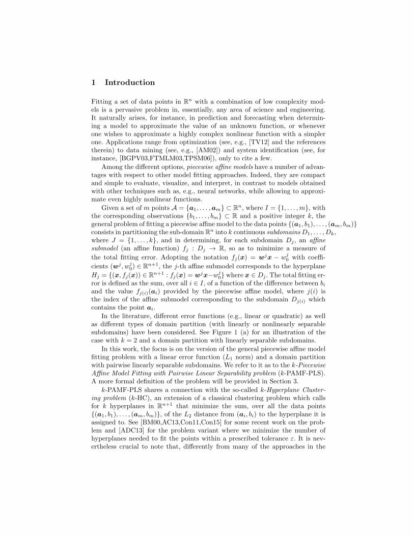
Fig. 2. (a) Pairwise linear separation of five linearly separable groups of points. (b)Classification with minimum misclassification error of two linearly inseparable groupsof points (note the misclassified black point).

thus corresponding to the largest violation among the inequalities (yj(i)−yj)ai−(y

j(i)0 − yj0) > 0. For an illustration, see Figure 2 (b).

Since the set of vectors (yj , yj0), for j ∈ J , satisfying constraint (yj(i)−yj)ai−(y

j(i)0 − yj0) > 0 is an open subset of Rn+1, it is common practice to replace it by

the inhomogeneous constraint (yj(i) − yj)ai − (yj(i)0 − yj0) ≥ 1, which induces a

closed feasible set. This can be done without loss of generality if we assume that

the norm of the vectors (yj(i), yj(i)0 ), (yj , yj0) can be arbitrarily large, for all j ∈ J .

Indeed, if (yj(i) − yj)ai − (yj(i)0 − yj0) > 0 but (yj(i) − yj)ai − (y

j(i)0 − yj0) < 1

for some ai ∈ A, then a feasible solution which satisfies the inhomogeneous

constraint can be obtained by just scaling (yj(i), yj(i)0 ) and (yj , yj0) by a constant

λ ≥ 1

(yj(i)−yj)ai−(yj(i)0 −yj

0). In the inhomogeneous version, the misclassification

error becomes:

max

{0, max

j∈J\{j(i)}

{1− (yj(i) − yj)ai + (y

j(i)0 − yj0)

}}. (3)

3.2 k-Piecewise affine model fitting problem with pairwise linearseparability

We can now provide a formal definition of k-Piecewise Affine Model Fitting withPairwise Linear Separability.

k-PAMF-PLS: Given a set of m points A = {a1, . . . ,am} ⊂ Rn with thecorresponding observations {b1, . . . , bm} ⊂ R and a positive integer k:

i) partition A into k subsets A1, . . . , Ak which are pairwise linearlyseparable via a domain partition D1, . . . , Dk of Rn induced, accordingto Equation (1), by a set of vectors (yj , yj0) ∈ Rn+1, for j ∈ J ,

ii) determine, for each subdomain Dj , an affine function fj : Dj → Rwhere fj(x) = wjx− wj

0 with parameters (wj , wj0) ∈ Rn+1,

so as to minimize the linear error function∑m

i=1 |bi − (wj(i)ai −wj(i)0 )|,

where j(i) ∈ J is the index for which ai ∈ Aj(i) ⊂ Dj(i).

4 Strengthened mixed-integer linear programmingformulation

In this section, we propose an MILP formulation to solve k-PAMF-PLS to opti-mality via branch-and-cut, as implemented in state-of-the-art MILP solvers. Toenhance the efficiency of the solution algorithm, we break the symmetries thatnaturally arise in the formulation by generating symmetry-breaking constraints.

Our MILP formulation is derived by combining a hyperplane clustering for-mulation (to partition the data points into k subsets A1, . . . , Ak and to determinean affine submodel for each of them) with multicategory linear classification con-straints (to guarantee a pairwise linearly separable domain partition D1, . . . Dk,consistent with the k subsets A1, . . . , Ak).

4.1 MILP formulation

For each i ∈ I and j ∈ J , we introduce a binary variable xij which takes value 1if the point ai is contained in the subset Aj and 0 otherwise. Let zi be the

fitting error of point ai ∈ A for each i ∈ I, (wj , wj0) ∈ Rn+1 the parameters of

the submodel of index j ∈ J , and (yj , yj0) ∈ Rn+1, with j ∈ J , the parametersused to enforce pairwise linear separability. Let also M1 and M2 be large enoughconstants (whose value is discussed below). The formulation is as follows:

min

m∑i=1

zi (4)

s.t.

k∑j=1

xij = 1 ∀i ∈ I (5)

zi ≥ bi −wjai + wj0 −M1(1− xij) ∀i ∈ I, j ∈ J (6)

zi ≥ −bi + wjai − wj0 −M1(1− xij) ∀i ∈ I, j ∈ J (7)

(yj1 − yj2)ai − (yj10 − yj2

0 ) ≥ 1−M2(1− xij1) ∀i ∈ I, j1, j2 ∈ J : j1 6= j2 (8)

xij ∈ {0, 1} ∀i ∈ I, j ∈ J (9)

zi ≥ 0 ∀i ∈ I (10)

(wj , wj0) ∈ Rn+1 ∀j ∈ J (11)

(yj , yj0) ∈ Rn+1 ∀j ∈ J. (12)

Constraints (5) guarantee that each point ai ∈ A be assigned to exactly one

submodel. Constraints (6) and (7) impose that zi = |bi−wj(i)ai+wj(i)0 |. Indeed,

together they imply that zi ≥ |bi−wjai +wj0|−M1(1−xij). When xij = 1, this

amounts to imposing zi ≥ |bi −wjai + wj0| (which will be tight in any optimal

solution due to the objective function direction), while being redundant (since

zi ≥ 0) when xij = 0 and M1 is large enough. For each j1 ∈ J , Constraints (8)impose that all the points assigned to the subsetAj1 (for which the term−M2(1−xij) vanishes) belong to the intersection of all the halfspaces defined by (yj1 −yj2)ai − (yj10 − yj20 ) ≥ 1, whereas they are deactivated when xij1 = 0 andM2 is sufficiently large. This way, we impose a zero misclassification error foreach data point, thus guaranteeing pairwise linear separability among the pointsassigned to the different submodels. Note that, if Constraints (8) are dropped, weobtain a relaxation corresponding to a k-hyperplane clustering problem wherethe objective function is measured according to (4), (6) and (7).

It is important to observe that, in principle, there exists no (large enough)finite value for the parameter M1 in Constraints (6) and (7). As an example,the fitting error between a point (a, b) = (e,−1) ∈ Rn+1, where e is the all-onevector, and the affine function f = wa− 1 is equal to ‖w‖1 (the L1 norm of w)and, thus, it is unbounded and arbitrarily large for an arbitrary large ‖w‖1. Letj(i) ∈ J such that xij(i) = 1. The introduction of a finite M1 corresponds toletting:

zi = max

j=j(i) and xij(i)=1︷ ︸︸ ︷|bi −wj(i)ai + w

j(i)0 |,

j 6=j(i) and xij=0︷ ︸︸ ︷max

j∈J\{j(i)}{|bi −wjai + wj

0| −M1}

, (13)

rather than zi = |bi − wj(i)ai + wj(i)0 |. Therefore, a finite M1 introduces a pe-

nalization term into the objective function, equal to:

m∑i=1

max

{0, max

j∈J\{j(i)}{|bi −wjai + wj

0| −M1} − |bi −wj(i)ai + wj(i)0 |

}. (14)

The effect is of penalizing solutions where the fitting error between any pointand any submodel is too large, regardless of the submodels to which each pointis assigned.

We face a similar issue for Constraints (8) due to the presence of the pa-rameter M2. Indeed, for any finite M2 and for xij1 = 0, the constraint implies

(yj1 − yj2)ai − (yj10 − yj20 ) ≥ 1 −M2. Hence, Constraints (8) impose that the

“linear distance”2 between each point ai and the hyperplane separating any pairof subdomains Dj1 , Dj2 be smaller than M2 − 1 even if ai is not contained ineither of the subdomains, i.e., even if ai /∈ Aj1 and ai /∈ Aj2 .

In spite of the lack of theoretically finite values for M1 and M2, setting themto a value a few orders of magnitude larger than the size of the box encapsulatingthe data points in Rn+1 typically suffices to produce good quality (if not optimal)solutions. We will mention an occurrence where this is not the case in Section 6.

2 Given a point a and a hyperplane of equation wx−w0 = 0, the distance from a tothe closest point belonging to the hyperplane amounts to |wa−w0|

‖w‖2. Then, the “linear

distance” mentioned in the text corresponds to the point-to-hyperplane distancemultiplied by ‖w‖2.

4.2 Symmetries

Let X ∈ {0, 1}m×k be the binary matrix with entries {X}ij = xij for i ∈ I andj ∈ J . We observe that Formulation (4)–(12) admits symmetric solutions as aconsequence of the existence of a symmetry group acting on the columns of X.This is because, for any X representing a feasible solution, an equivalent solutioncan be obtained by permuting the columns of X, an operation which correspondsto permuting the labels 1, . . . , k by which the submodels and subdomains areindexed.

From a computational point of view, the solvability of our MILP formu-lation for k-PAMF-PLS is hindered by the existence of symmetries. On theone hand, this is because, when adopting methods based on branch-and-bound,symmetries typically lead to an unnecessarily large search tree where equiva-lent (symmetric) solutions are discovered again and again at different nodes.On the other hand, the presence of symmetries usually leads to weaker Lin-ear Programming (LP) relaxations, for which the barycenter of each set ofsymmetric solutions, which often yields very poor LP bounds, is always fea-sible [KP08]. This is the case of our formulation where, for a sufficiently largeM = M1 = M2 ≥ k

k−1 max{1, |b1|, |b2|, . . . , |bm|}, the LP relaxation of Formu-

lation (4)–(12) admits a solution of value 0. To see this, let xij = 1k for all

i ∈ I, j ∈ J . Constraints (5) are clearly satisfied. Let then zi = 0 for all i ∈ I,(wj , wj

0) = (0, 0) and (yj , yj0) = (0, 0) for all j ∈ J . Constraints (6), (7), and (8)are then satisfied whenever we have, respectively, M1

k−1k ≥ bi, M1

k−1k ≥ −bi,

and M2k−1k ≥ 1.

A way to deal with this issue is to partition the set of feasible solutionsinto equivalence classes (or orbits) under the symmetry group, selecting a sin-gle representative per class. Different options are possible. We refer the readerto [Mar10] for an extensive survey on symmetry in mathematical programming.A possibility, originally introduced in [MDZ01,MDZ06], is of selecting as a rep-resentative the (unique) feasible solution of each orbit where the columns of Xare lexicographically sorted in non-increasing order. According to [KP08], we callthe convex hull of such lexicographically sorted matrices X ∈ {0, 1}n×k orbitope.

4.3 Symmetry breaking constraints from the partitioning orbitope

Since, in our case, X is a partitioning matrix (a matrix X ∈ {0, 1}n×k withexactly a 1 per row), we are interested in the so-called partitioning orbitope,whose complete linear description is given in [KP08].

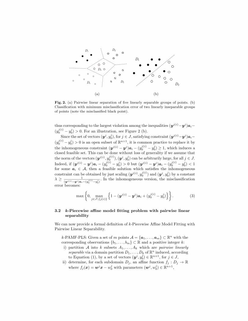
Neglecting the trivial constraints, the partitioning orbitope is defined by theset of so-called Shifted Column Inequalities (SCIs). Call B(i,j) a bar, definedas B(i,j) = {(i, j), (i, j + 1), . . . , (i,min{i, k})}, and col(i,j) a column, definedas col(i,j) = {(j, j), (j + 1, j), ..., (i, j)}. A shifted column S(i,j) is a subset ofthe indices of X obtained by shifting some of the indices in col(i,j) diagonallytowards the upper-left portion of X. For an illustration, see Figure 3. For two

i

j

η

i

j

i

j

(a) (b) (c)

Fig. 3. (a) The bar B(i,j) (in black and dark gray) and the column col(i−1,j−1) (in lightgray). (b) and (c) Two shifted columns (in light gray) obtained by shifting col(i−1,j−1).Note how the shifting operation introduces empty rows.

subsets of indices B(i,j), S(i−1,j−1) ⊂ I × J thus defined, an SCI reads:∑(i′,j′)∈B(i,j)

xi′j′ −∑

(i′,j′)∈S(i−1,j−1)

xi′j′ ≤ 0.

As shown in [KP08], the linear description of the partitioning orbitope is:

k∑j=1

xij = 1 ∀i ∈ I (15)

∑(i′,j′)∈B(i,j)

xi′j′ −∑

(i′,j′)∈S(i−1,j−1)

xi′j′ ≤ 0 ∀B(i,j), S(i−1,j−1) (16)

xij = 0 ∀i ∈ I, j ∈ J : j ≥ i + 1 (17)

xij ≥ 0 ∀i ∈ I, j ∈ J, (18)

where Constraints (16) are SCIs, while Constraints (17) restrict the problem tothe only elements of X that are either on the main diagonal or below it.

Although there are exponentially many SCIs, the corresponding separationproblem can be solved in linear time by dynamic programming, as shown in [KP08].

When solving the MILP formulation (4)–(12) with a branch-and-cut algo-rithm, we generate maximally violated SCIs both at each node of the enumera-tion tree (by separating the corresponding fractional solution) and every time anew integer solution is found (thus separating the integer incumbent solution).

5 Four-step heuristic algorithm

As we will see in Section 6, the introduction of SCIs has a remarkable impacton the solution times. Nevertheless, even with them the MILP formulation onlyallows to solve small to medium size instances in a reasonable amount of com-puting time.

To tackle instances of larger size, we propose an efficient heuristic that takesinto account all the aspects of the problem at each iteration by alternately and

coordinately solving a sequence of subproblems, namely, affine submodel fitting,point partition, and domain partition, as explained in detail in the following.Differently from other heuristic approaches in the literature (see Section 2), thedomain partitioning aspect is considered at each iteration, rather than deferredto a final stage.

We start from a feasible solution composed of a point partition A1, . . . , Ak,a domain partition D1, . . . , Dk (induced by the parameters (yj , yj0) for j ∈ J),

and a set of affine submodels of parameters (wj , wj0), for j ∈ J . Iteratively, the

algorithm tries to improve the current solution by applying the following foursteps (until convergence or until a time limit is met):

i) Submodel Fitting: Given the current point partition A1, . . . , Ak of A ={a1, . . . ,am}, determine for each j ∈ J an affine submodel with parame-ters (wj , wj

0) that minimize the linear fitting error over all the data points{(a1, b1), . . . , (am, bm)} ⊂ Rn+1. As we shall see, this is carried out by solvinga single linear program.

ii) Point Partition: Given the current set of affine submodels fj : Dj → Rwith fj(x) = wjx − wj

0 and j ∈ J , identify a set of critical data points(ai, bi) ∈ Rn+1 and (re)assign them to other submodels in an attempt toimprove (decrease) the total linear fitting error over all the dataset. As de-scribed below, the identification and reassignment of such points is based onan ad hoc criterion and on a related control parameter.

iii) Domain Partition: Given the current point partition A1, . . . , Ak of A ={a1, . . . ,am}, a multicategory linear classification problem is solved via Lin-ear Programming to either find a pairwise linearly separable domain parti-tion D1, . . . , Dk of Rn, consistent with the current point partition, or, if noneexists, to construct a domain partition which minimizes the total misclassi-fication error. In the latter case, i.e., when there is at least an index j ∈ Jfor which Aj 6⊂ Dj , we say that the previously constructed point partitionis not consistent with the resulting domain partition D1, . . . , Dk.

iv) Partition Consistency: If the current point partition and domain parti-tion are inconsistent, the former is modified to make it consistent with thelatter. For every index j ∈ J and every misclassified point ai (if any) be-longing to Aj (i.e., for any ai ∈ A where ai ∈ Aj and ai ∈ Dj′ , for somej, j′ ∈ J such that j 6= j′), ai is reassigned to the subset Aj′ associated withDj′ .

In the following, we describe the four steps in greater detail.

In the Submodel Fitting step, we determine, for each j ∈ J , the submodelparameters (wj , wj

0) yielding the smallest fitting error by solving the following

linear program:

min

m∑i=1

di (19)

s.t. di ≥ bi −wj(i)ai + wj(i)0 ∀i ∈ I (20)

di ≥ −bi + wj(i)ai + wj(i)0 ∀i ∈ I (21)

(wj , wj0) ∈ Rn+1 ∀j ∈ J (22)

di ≥ 0 ∀i ∈ I, (23)

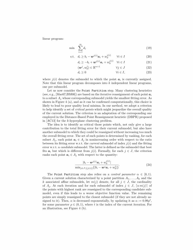
where j(i) denotes the submodel to which the point ai is currently assigned.Note that this linear program decomposes into k independent linear programs,one per submodel.

Let us now consider the Point Partition step. Many clustering heuristics(see, e.g., [Mac67,BM00]) are based on the iterative reassignment of each point ai

to a subset Aj whose corresponding submodel yields the smallest fitting error. Asshown in Figure 4 (a), and as it can be confirmed computationally, this choice islikely to lead to poor quality local minima. In our method, we adopt a criterionto help identify a set of critical points which might jeopardize the overall qualityof the current solution. The criterion is an adaptation of the corresponding oneemployed in the Distance-Based Point Reassignment heuristic (DBPR) proposedin [AC13] for the k-hyperplane clustering problem.

The idea is to identify as critical those points which, not only give a largecontribution to the total fitting error for their current submodel, but also haveanother submodel to which they could be reassigned without increasing too muchthe overall fitting error. The set of such points is determined by ranking, for eachsubset Aj , each point ai ∈ Aj in nonincreasing order with respect to the ratiobetween its fitting error w.r.t. the current submodel of index j(i) and the fittingerror w.r.t. a candidate submodel. The latter is defined as the submodel that bestfits ai but which is different from j(i). Formally, for each j ∈ J , the criterionranks each point ai ∈ Aj with respect to the quantity:

|bi −wj(i)ai + wj(i)0 |

minj∈J\{j(i)}{|bi −wjai + wj0|}. (24)

The Point Partition step also relies on a control parameter α ∈ [0, 1).Given a current solution characterized by a point partition A1, . . . , Ak and thek associated affine submodels, let m(j) denote, for all j ∈ J , the cardinalityof Aj . At each iteration and for each submodel of index j ∈ J , dαm(j)e ofthe points with highest rank are reassigned to the corresponding candidate sub-model, even if this leads to a worse objective function value. The remainingpoints are simply reassigned to the closest submodel (if they are not already as-signed to it). Then, α is decreased exponentially, by updating it as α := 0.99ρt,for some parameter ρ ∈ (0, 1), where t is the index of the current iteration. Foran illustration, see Figure 4 (b).

D1

D2

a1

ai

bi

D1

D2

a1

ai

bi

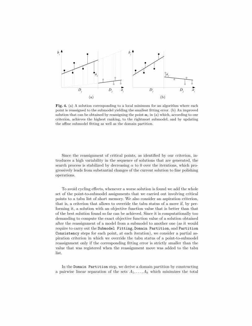
(a) (b)

Fig. 4. (a) A solution corresponding to a local minimum for an algorithm where eachpoint is reassigned to the submodel yielding the smallest fitting error. (b) An improvedsolution that can be obtained by reassigning the point a1 in (a) which, according to ourcriterion, achieves the highest ranking, to the rightmost submodel, and by updatingthe affine submodel fitting as well as the domain partition.

Since the reassignment of critical points, as identified by our criterion, in-troduces a high variability in the sequence of solutions that are generated, thesearch process is stabilized by decreasing α to 0 over the iterations, which pro-gressively leads from substantial changes of the current solution to fine polishingoperations.

To avoid cycling effects, whenever a worse solution is found we add the wholeset of the point-to-submodel assignments that we carried out involving criticalpoints to a tabu list of short memory. We also consider an aspiration criterion,that is, a criterion that allows to override the tabu status of a move if, by per-forming it, a solution with an objective function value that is better than thatof the best solution found so far can be achieved. Since it is computationally toodemanding to compute the exact objective function value of a solution obtainedafter the reassignment of a model from a submodel to another one (as it wouldrequire to carry out the Submodel Fitting, Domain Partition, and Partition

Consistency steps for each point, at each iteration), we consider a partial as-piration criterion in which we override the tabu status of a point-to-submodelreassignment only if the corresponding fitting error is strictly smaller than thevalue that was registered when the reassignment move was added to the tabulist.

In the Domain Partition step, we derive a domain partition by constructinga pairwise linear separation of the sets A1, . . . , Ak which minimizes the total

misclassification error. This is achieved by solving the following linear program:

min

m∑i=1

ei (25)

s.t. ei ≥ −(yj(i) − yj)ai + (yj(i)0 − yjo) + 1 ∀i ∈ I, j ∈ J \ {j(i)} (26)

ei ≥ 0 ∀i ∈ I (27)

(yj , yj0) ∈ Rn+1 ∀j ∈ J, (28)

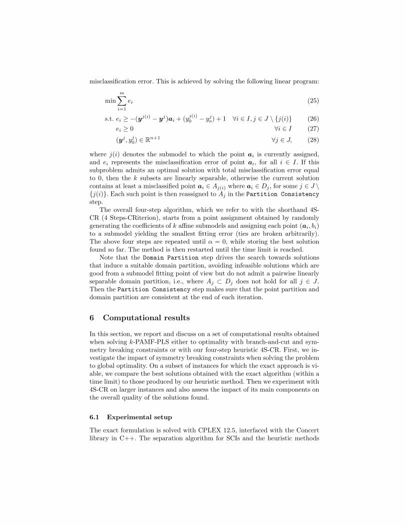
where j(i) denotes the submodel to which the point ai is currently assigned,and ei represents the misclassification error of point ai, for all i ∈ I. If thissubproblem admits an optimal solution with total misclassification error equalto 0, then the k subsets are linearly separable, otherwise the current solutioncontains at least a misclassified point ai ∈ Aj(i) where ai ∈ Dj , for some j ∈ J \{j(i)}. Each such point is then reassigned to Aj in the Partition Consistency

step.The overall four-step algorithm, which we refer to with the shorthand 4S-

CR (4 Steps-CRiterion), starts from a point assignment obtained by randomlygenerating the coefficients of k affine submodels and assigning each point (ai, bi)to a submodel yielding the smallest fitting error (ties are broken arbitrarily).The above four steps are repeated until α = 0, while storing the best solutionfound so far. The method is then restarted until the time limit is reached.

Note that the Domain Partition step drives the search towards solutionsthat induce a suitable domain partition, avoiding infeasible solutions which aregood from a submodel fitting point of view but do not admit a pairwise linearlyseparable domain partition, i.e., where Aj ⊂ Dj does not hold for all j ∈ J .Then the Partition Consistency step makes sure that the point partition anddomain partition are consistent at the end of each iteration.

6 Computational results

In this section, we report and discuss on a set of computational results obtainedwhen solving k-PAMF-PLS either to optimality with branch-and-cut and sym-metry breaking constraints or with our four-step heuristic 4S-CR. First, we in-vestigate the impact of symmetry breaking constraints when solving the problemto global optimality. On a subset of instances for which the exact approach is vi-able, we compare the best solutions obtained with the exact algorithm (within atime limit) to those produced by our heuristic method. Then we experiment with4S-CR on larger instances and also assess the impact of its main components onthe overall quality of the solutions found.

6.1 Experimental setup

The exact formulation is solved with CPLEX 12.5, interfaced with the Concertlibrary in C++. The separation algorithm for SCIs and the heuristic methods

are implemented in C++ and compiled with GNU-g++-4.3. SCIs are addedto the default branch-and-cut algorithm implemented in CPLEX via both alazy constraint callback and a user cut callback, thus separating SCIs for bothinteger and fractional solutions. This way, with lazy constraints we guaranteethe lexicographic maximality of the columns of the partitioning matrix X forany feasible solution found by the method. With user cuts, we also allow forthe introduction of SCIs at the different nodes of the branch-and-cut tree, thustightening the LP relaxations. In 4S-CR (and its variants, as introduced in thefollowing), the Submodel Fitting and Domain Partition steps are carried outby solving the corresponding LPs, namely (19)–(23) and (25)–(28), with CPLEX.

The experiments are conducted on a Dell PowerEdge Quad Core Xeon 2.0 Ghz,with 16 GB of RAM. In the heuristics, we set ρ = 0.5 and adopt a tabu list witha short memory of two iterations.

6.2 Test instances

We consider both a set of structured, randomly generated instances, as well assome real-world ones taken from the UCI repository [FA13].

We classify the random instances into four groups: small (m = 20, 30, 40,50, 60, 75, 100 and n = 2, 3, 4, 5), medium (m = 500 and n = 2, 3, 4, 5), andlarge (m = 1000 and n = 2, 3, 4, 5)3. They are constructed by randomly sam-pling the data points ai and the corresponding observations bi from a randomlygenerated (discontinuous) piecewise affine model with k = 5 pieces and an ad-ditional Gaussian noise. First, we generate k subdomains D1, . . . , Dk by solvinga multiway linear classification problem on k randomly chosen representativepoints in Rn. Then, we randomly choose the submodel parameters (wj , wj

0) forall j ∈ J and sample, uniformly at random, the m points {a1, . . . ,am} ∈ Rn.For each sampled point ai, we keep track of the subdomain Dj(i) which containsit and set bi to the value that the affine submodel of index j(i) takes in ai, i.e.,

wj(i)ai−wj(i)0 . Then, we add to bi an additive Gaussian noise with 0 mean and

a variance which is chosen, for each submodel, by sampling uniformly at randomwithin [ 7

10 ·3

1000 ,3

1000 ]. For convenience, but w.l.o.g., after an instance has beenconstructed, we rescale all its data points (and their observations) so that theybelong to [0, 10]n+1.

As to the real-world instances, we consider four datasets from the UCI reposi-tory: Auto MPG (auto), Breast Cancer Wisconsin Original (breast), ComputerHardware (cpu), and Housing (house). We remove data points with missingfeatures, convert each categorical attribute (if any) to a numerical value, andnormalize the data so that each point belongs to the interval [0, 10]n+1. We thenperform feature extraction via Principal Component Analysis (PCA), using the

3 We do not consider instances with n = 1 since k-PAMF-PLS is pseudopolynomiallysolvable in this case. Indeed, if the domain coincides with R, then the number oflinear domain partitions is, at most, O(mk). An optimal solution to k-PAMF-PLScan thus be found by constructing all such partitions and then solving, for each ofthem, an affine model fitting problem in polynomial time by Linear Programming.

Matlab toolbox PRTools, calling the function PCAM(A,0.9), where A is the Mat-lab data structure where the data points are stored. After preprocessing, theinstances are of the following size: m = 397, n = 3 (auto), m = 698, n = 5(breast), m = 209, n = 5 (cpu), and m = 506, n = 8 (house).

All the instances are solved with different values of k, namely, k = 2, 3, 4, 5.This way, the experiments are in line with a real-world scenario where the com-plexity of the underlying model is unknown.

Throughout the section, speedup factors and average improvements will bereported as ratios of geometric means.

6.3 Exact solutions via the MILP formulations

We test our MILP formulation with and without SCIs on the small dataset,considering four figures:

– total computing time (in seconds) needed to solve the problem, includingthe generation of SCIs as symmetry breaking constraints (Time);

– total number of branch-and-bound nodes that have been generated, dividedby 1000 (Nodes[k]);

– percent gap at the end of the computations (Gap), defined as 100 |LB−UB|10−4+|LB| ,

where LB and UB are the tightest lower and upper bounds that have beenfound; if LB = 0, a “-” is reported;

– total number of generated symmetry breaking constraints (Cuts).

The instances are solved for k = 2, 3, 4, 5, within a time limit of 3600 seconds.We run CPLEX in deterministic mode on a single thread with default settings.In all the cases, we set M = M1 = M2 = 1000.

The results are reported in Tables 1 for k = 2, 3 and in Table 2 for k = 4, 5.In the second table, we omit the results for the instances with n = 4, 5 as, bothwith or without SCIs, no solutions with a finite gap are found within the timelimit (i.e., the lower bound LB is always 0). Note that, for k = 2, symmetry isbroken by just fixing the top left element of the matrix X to 1, i.e., by letting,w.l.o.g., x11 = 1. Hence, we do not resort to the generation of SCIs in this case.

Let us neglect the case of k = 2 and focus on the full set of 56 k-PAMF-PLS problems that are considered for this dataset (28 instances for k = 3 and14 for k = 4, 5). Without SCI inequalities, we achieve an optimal solution in24 cases out of 56 (43%). The introduction of SCIs has a very positive impact.They allow to solve to optimality 10 more instances, for a total of 34 (60.1%).SCIs also yield a substantial reduction in both computing time and numberof nodes. When focusing on the 24 instances solved by both variants of thealgorithm, the overall results show that the introduction of SCIs yields a speedup,on (geometric) average, of almost 3 times, corresponding to a reduction of 66%of the computing times. The number of nodes is reduced by the same factorof 66%. Interestingly, this improvement is obtained by adding a rather smallnumber of cuts which, in practice, prove to be highly effective. See, e.g., theinstance with m = 40, n = 3 which, when solved for k = 3 with SCIs, presents

Table 1. Results obtained on the small dataset when solving the MILP formulation fork = 2 (without SCIs) and for k = 3 (with and without SCIs). For k = 3 and for eachinstance, if both variants achieve an optimal solution, the smallest number of nodesand computing time are highlighted in boldface. If at least a variant does not achievean optimal solution, the smallest gap is highlighted.

k=2 k=3

without SCIs without SCIs with SCIs

n m Time Nodes[k] Gap Time Nodes[k] Gap Time Nodes[k] Gap Cuts

2 20 0.1 0.2 0.0 2.3 2.0 0.0 2.1 1.1 0.0 122 30 0.7 0.5 0.0 4.8 6.5 0.0 4.3 5.0 0.0 102 40 0.7 0.7 0.0 7.9 11.3 0.0 4.1 4.0 0.0 182 50 0.8 0.6 0.0 9.3 9.8 0.0 4.0 5.2 0.0 172 60 1.2 1.0 0.0 14.7 17.9 0.0 8.7 8.3 0.0 82 75 2.4 1.2 0.0 20.2 20.7 0.0 8.8 7.7 0.0 82 100 3.8 1.7 0.0 43.6 28.9 0.0 43.1 28.4 0.0 13

3 20 0.4 0.9 0.0 13.9 29.0 0.0 5.6 9.3 0.0 73 30 0.7 1.2 0.0 58.3 124.4 0.0 35.6 55.1 0.0 203 40 1.8 2.2 0.0 226.9 291.7 0.0 49.1 64.6 0.0 193 50 1.5 3.1 0.0 603.6 467.0 0.0 117.7 122.2 0.0 153 60 4.7 5.1 0.0 615.9 440.3 0.0 171.5 147.8 0.0 223 75 5.4 7.4 0.0 3600.0 802.4 76.7 512.7 324.8 0.0 293 100 9.9 19.6 0.0 3600.0 757.1 89.4 3196.2 1272.8 0.0 42

4 20 1.2 2.3 0.0 131.0 270.1 0.0 35.2 84.0 0.0 104 30 2.1 3.8 0.0 633.1 802.8 0.0 167.8 224.8 0.0 114 40 5.6 11.1 0.0 3600.0 1519.4 79.3 3345.2 1867.2 0.0 214 50 8.6 20.8 0.0 3600.0 1096.8 - 3600.0 1206.0 85.3 194 60 15.2 39.0 0.0 3600.0 970.8 - 3600.0 1238.7 89.7 224 75 50.3 87.1 0.0 3600.0 851.1 - 3600.0 1014.9 86.6 174 100 98.9 192.3 0.0 3600.0 529.5 - 3600.0 508.1 - 26

5 20 1.9 5.6 0.0 679.6 974.1 0.0 170.0 311.7 0.0 115 30 6.3 16.2 0.0 3600.0 1775.3 - 3600.0 2054.0 73.3 185 40 27.7 61.4 0.0 3600.0 1422.8 - 3600.0 1363.3 - 135 50 54.4 125.6 0.0 3600.0 1118.3 - 3600.0 1132.1 - 245 60 491.2 830.6 0.0 3600.0 963.5 - 3600.0 1009.1 - 175 75 1751.1 1841.4 0.0 3600.0 788.0 - 3600.0 815.1 - 175 100 3600.0 3649.2 9.3 3600.0 769.3 - 3600.0 623.1 - 32

Table 2. Results obtained on the small dataset when solving the MILP formulationfor k = 4, 5 with and without SCIs. For each instance, if both variants achieve anoptimal solution, the smallest number of nodes and computing time are highlighted inboldface. If at least a variant does not achieve an optimal solution, the smallest gap ishighlighted.

k=

4k=

5

wit

houth

SC

Isw

ith

SC

Isw

ithout

SC

Iw

ith

SC

I

nn

Tim

eN

odes

[k]

Gap

Tim

eN

odes

[k]

Gap

Cuts

Tim

eN

odes

[k]

Gap

Tim

eN

odes

[k]

Gap

Cuts

220

7.6

12.9

0.0

4.5

4.0

0.0

27

112.2

152.4

0.0

31.1

35.3

0.0

268

230

31.6

41.9

0.0

7.2

9.0

0.0

39

554.8

441.3

0.0

59.6

48.2

0.0

397

240

105.8

115.3

0.0

19.0

18.6

0.0

86

3600.0

1308.2

28.7

98.2

75.1

0.0

472

250

156.0

145.3

0.0

35.8

39.6

0.0

174

3600.0

1347.0

20.3

347.4

153.2

0.0

893

260

411.9

275.1

0.0

244.1

143.0

0.0

86

3600.0

865.1

90.2

1062.9

453.1

0.0

783

275

520.9

328.3

0.0

158.5

118.0

0.0

155

3600.0

577.0

97.6

2385.9

739.7

0.0

1034

2100

3600.0

673.3

15.7

367.0

169.6

0.0

233

3600.0

356.0

98.6

3600.0

319.2

98.2

1105

320

1067.9

1246.5

0.0

118.8

176.2

0.0

67

3600.0

2306.5

-2013.0

1401.2

0.0

428

330

3600.0

1590.5

-2336.6

1480.7

0.0

125

3600.0

1491.6

-3600.0

1236.9

-825

340

3600.0

1188.1

-3600.0

1344.4

34.2

91

3600.0

1077.4

-3600.0

871.3

-385

350

3600.0

896.5

-3600.0

847.6

94.4

174

3600.0

738.2

-3600.0

704.0

-496

360

3600.0

754.1

-3600.0

697.5

-120

3600.0

725.4

-3600.0

597.2

-580

375

3600.0

626.7

-3600.0

458.8

-187

3600.0

444.9

-3600.0

331.0

-843

3100

3600.0

440.5

-3600.0

370.5

-267

3600.0

324.4

-3600.0

221.4

-1691

a speedup in the computing time, when compared to the case without SCIs, of4.6 times (corresponding to a reduction of 78%) with the sole introduction of 19symmetry breaking constraints.

In our preliminary experiments, we observed the generation of a higher num-ber of cuts when employing older versions of CPLEX, such as 12.1 and 12.2whereas, with CPLEX 12.5, their number is significantly smaller. This is, mostlikely, a consequence of the introduction of more aggressive techniques for sym-metry detection and symmetry breaking in the latest versions of CPLEX. Wenevertheless remark that the improvement in computing time provided by theintroduction of SCIs appears to be comparable for all the versions of CPLEX 12,regardless of the number of cuts that are generated.

Although the introduction of SCIs clearly increases the number of instanceswhich can be solved to optimality, the results in Tables 1 and 2 show thatthe exact approach via mixed-integer linear programming might require largecomputing times even for fairly small instances with n ≥ 3 and m ≥ 40 fork ≥ 4. For k = 2, all the instances are solved to optimality, with the soleexception of the instance with m = 100, n = 5 (which reports a gap of 9.3%).For k = 3, Table 1 shows that, already for n = 4 and m ≥ 50, the gap after onehour is still larger than 80%. According to Table 2, the exact approach becomesimpractical for n = 3 and m ≥ 40 for k = 4, and for n = 3 and m ≥ 30 fork = 5.

6.4 Comparison between the four-step heuristic 4S-CR and theMILP formulation

Before assessing the effectiveness of 4S-CR on larger instances, we compare thesolutions it provides with the best ones found via mixed-integer linear program-ming on the small dataset (within the time limit). The results are reported inTable 3. For a fair comparison, 4S-CR is run, for the instances that are solvedto optimality by the exact method, for the same time taken by the latter. Forthe instances for which an optimal solution has not been found, 4S-CR is runup to the time limit of 3600 seconds.

When comparing the quality of the solutions found by 4S-CR with thosefound by the MILP formulation with SCIs, we register, for k = 2, very close tooptimal solutions with, on (geometric) average, a 4% larger fitting error. Thisnumber decreases to 1% for k = 3. For larger values of k, namely k = 4 andk = 5, for which the number of instances that are unsolved when adopting theMILP formulation is much larger, 4S-CR yields solutions that are much betterthan those found via mixed-integer linear programming. When neglecting theinstances with an optimal solution of value 0 (which would skew the geometricmean), the solutions provided by 4S-CR are, on geometric average, better thanthose obtained via the exact method by 14% for k = 4 and by 20% for k = 5.

For k = 2, 3, 4, 5, 4S-CR finds equivalent or better solutions that those ob-tained via mixed-integer linear programming in, respectively, 11, 15, 18, and19 cases, with strictly better solutions in, respectively, 1, 5, 16, and 15 cases.

Table 3. Comparison between the best results obtained for k = 2, 3, 4, 5 on the smallinstances when solving the MILP formulation (with symmetry breaking constraintsand within a time limit of 3600 seconds) and those obtained via 4S-CR. The latter isrun for as much time as that required to solve the MILP formulation (within the timelimit). For each instance, the value of the best solution found is highlighted in boldface.

k = 2 k = 3 k = 4 k = 5

Objective Objective Objective Objectiven m Time MILP 4S-CR Time MILP 4S-CR Time MILP 4S-CR Time MILP 4S-CR

2 20 0.1 18.3 22.4 2.1 9.6 9.6 4.5 6.1 7.1 31.1 4.5 6.12 30 0.1 30.5 30.5 4.3 19.3 19.3 7.2 10.0 10.0 59.6 7.7 8.82 40 0.5 61.3 61.3 4.1 37.8 45.4 19.0 24.7 35.5 98.2 14.8 21.22 50 0.3 56.0 56.0 4.0 39.1 40.9 35.8 26.9 29.5 347.4 22.1 22.12 60 1.2 86.6 91.7 8.7 53.1 61.8 244.1 43.2 53.1 1062.9 35.7 43.52 75 1.7 40.5 45.4 8.8 31.3 31.6 158.5 28.6 30.5 2385.9 27.3 28.42 100 1.6 114.9 114.9 43.1 62.9 62.9 367.0 48.4 48.5 3600.0 187.4 48.4

3 20 0.3 11.3 11.3 5.6 4.3 4.6 118.8 2.3 2.4 2013.0 0.4 0.93 30 0.7 14.1 13.8 35.6 9.4 9.0 2336.6 6.3 6.3 3600.0 4.5 4.73 40 2.9 29.3 32.3 49.1 19.6 21.2 3600.0 14.7 15.5 3600.0 11.7 11.73 50 2.0 48.6 55.5 117.7 26.3 26.3 3600.0 20.2 17.9 3600.0 21.2 15.13 60 4.9 40.0 40.0 171.5 22.7 25.0 3600.0 22.7 17.5 3600.0 17.3 12.93 75 5.9 72.5 82.4 512.7 43.9 47.9 3600.0 35.2 31.6 3600.0 54.0 31.53 100 10.3 86.5 88.0 3196.2 51.3 51.3 3600.0 77.2 33.6 3600.0 69.2 33.2

4 20 1.2 7.5 7.5 35.2 2.3 2.3 3600.0 0.2 0.3 2.1 0.0 0.44 30 1.2 20.0 20.3 167.8 6.8 6.8 3600.0 3.5 3.4 3600.0 1.3 1.44 40 4.1 34.4 34.4 3345.2 16.5 16.5 3600.0 11.0 10.3 3600.0 7.4 6.84 50 6.2 38.0 38.0 3600.0 20.5 20.0 3600.0 19.0 13.4 3600.0 17.7 6.34 60 12.1 40.1 41.0 3600.0 28.8 27.3 3600.0 24.8 17.9 3600.0 21.1 15.54 75 23.0 85.0 88.5 3600.0 49.4 53.9 3600.0 50.4 37.8 3600.0 46.1 32.44 100 57.0 110.3 118.0 3600.0 113.9 74.0 3600.0 139.3 49.7 3600.0 117.6 43.3

5 20 2.6 8.9 8.9 170.0 0.5 0.5 0.3 0.0 0.5 0.6 0.0 0.05 30 4.0 17.1 19.2 3600.0 6.7 6.7 3600.0 1.9 1.7 3600.0 0.3 0.65 40 12.1 37.9 41.7 3600.0 18.7 19.5 3600.0 13.3 8.9 3600.0 6.7 5.15 50 32.0 28.9 29.4 3600.0 21.7 17.9 3600.0 15.8 12.4 3600.0 9.7 8.45 60 457.1 58.4 58.6 3600.0 43.9 44.0 3600.0 37.5 31.9 3600.0 33.6 21.25 75 820.9 62.6 65.0 3600.0 26.7 29.4 3600.0 50.9 20.7 3600.0 53.0 18.45 100 3600.0 79.3 84.1 3600.0 56.0 60.8 3600.0 60.5 49.3 3600.0 61.6 42.9

Overall, when considering the instances jointly, 4S-CR performs as good or bet-ter than mixed-integer linear programming in 63 cases out of 112 (28 instances,each solved 4 times, once per value of k), strictly improving over the latter in 37cases. This indicates that the quality of the solutions found via 4S-CR can bequite high even for small-size instances and that the difference w.r.t. the exactmethod, at least on the instances for which a comparison is viable, seems to beincreasing with the number of points m, the number of dimensions n, and thenumber of submodels k.

Note that, for the instance with m = 30, n = 3 and for both k = 2 and k = 3,the MILP formulation yields, in strictly less than the time limit, a solution whichis worse than the corresponding one found by 4S-CR. As discussed in Section 4,this is most likely due to the selection of too small values for the parameters M1

and M2. Experimentally, we observed that the issue can be avoided by choosingM = M1 = M2 = 10000, although at the cost of a substantially larger computingtime (due to the need for a higher numerical precision to handle the largerdifferences between the magnitudes of the coefficients in the formulation).

6.5 Experiments with 4S-CR on larger instances and impact of themain 4S-CR features

We now present the results obtained with 4S-CR on larger instances and assessthe impact of the main features of 4S-CR (i.e., the criterion for identifying andreassigning critical points in the Point Partition step, the Domain Partition

step, and the Partition Consistency step, applied at each iteration) on thequality of the solutions found.

As already mentioned, we set ρ = 0.5 in all the experiments involving ourcriterion for identifying critical points and we consider a tabu list with a memoryof two iterations. When tuning the parameters, we observed improved results onthe smaller instances when increasing ρ, as opposed to worse ones on the largerinstances. This is, most likely, a consequence of the number of iterations carriedout within the time limit, which becomes much smaller for a larger value of ρ,thus forcing the method to halt with a solution which is too close to the startingone. As to the tabu list, we observed that a short memory of two iterationssuffices to prevent loops. Indeed, due to the nature of the problem as well as dueto the many aspects of k-PAMF-PLS that our method considers, the values of theparameters of the piecewise-affine submodels change often dramatically withinvery few iterations. This way, few iterations taking place after a worsening movetypically suffice to prevent that a point-to-submodel reassignment take placetwice, thus making the occurrence of loops extremely unlikely.

To assess the impact of the Point Partition step based on the criterionfor critical points (and on the corresponding control parameter), we introduce avariant of 4S-CR where, in the former step, every point (ai, bi) is (re)assigned toa submodel yielding the smallest fitting error. This is in line with many popularclustering heuristics, as reported in Section 2. We refer to this method as 4S-CL(where “CL” stands for “closest”).

To evaluate the relevance of considering, in 4S-CR, the domain partitionaspect directly at each iteration (via the Domain Partition and Partition

Consistency steps), we also consider a standard (STD) two-phase method which,first, addresses the clustering aspect of k-PAMF-PLS and, only at the end, be-fore halting, takes the domain partition aspect into account. In the algorithm,which we consider in two versions, we iteratively alternate between the SubmodelFitting and Point Partition steps. In the latter step, we either reassign everypoint to the “closest” submodel (STD-CL) or to that indicated by our criterion(STD-CR). After a local minimum has been reached, a pairwise linearly separa-ble domain partition with minimum misclassification error is derived by solvinga multiway linear classification problem via linear programming, as in Prob-lem (25)–(28).

Since STD-CL is similar to most of the standard techniques proposed in theliterature (see Section 2), we consider it as the baseline method and compare theother methods (4S-CR, 4S-CL, and STD-CR) to it. The results for the medium,large, and UCI datasets, obtained with a time limit of, respectively, 900, 1800,and 900 seconds, are reported in Table 4.

The comparison shows that 4S-CR outperforms the baseline method STD-CLin almost all the cases. When considering the medium instances, 4S-CR yieldsan improvement in objective function value of, on geometric average, 8%, 21%,21%, and 24% for, respectively, k = 2, 3, 4, and 5. On the large instances, theimprovement is of 16%, 24%, 29%, and 24%. For the four UCI instances, theimprovement is of 6%, 9%, 13%, and 16%. When considering the three datasetsjointly, the improvement is of 8%, 21%, 21%, 24%. On geometric average, forall the values of k, 4S-CR improves on the fitting error of STD-CL by 20%. Ona total of 112 instances (for the different values of k) of k-PAMF-PLS, 4S-CRachieves the best solution in 103 cases (92%).

When comparing 4S-CL to STD-CL, we register, on geometric mean andfor the different values of k, an improvement of 4%, 9%, 10%, and 16% for themedium instances, of 12%, 17%, 17%, and 11% for the large ones, and of 4%,9%, 10%, and 16% on the UCI datasets. When considering all the datasets andall the values of k jointly, the improvement is of 12%. Although still substantial,this value is not as large as that for 4S-CR, thus highlighting the relevance of thecriterion based on critical points that is adopted in the Point Partition step.At the same time, it also shows that, even without the criterion, the central ideaof 4S-CR (i.e., considering the domain partition aspect of the problem directlyat each iteration, rather than deferring it to a final phase) has a large positiveimpact on the solution quality.

Most interestingly, the results for STD-CR are quite poor. When consideringall the 112 instances (for the different values of k), the method yields, on geo-metric average, a 4% larger fitting error w.r.t. STD-CL. This is not surprisingas, by constructing a domain partition only at the very end of the algorithm,the solutions that are obtained before its derivation typically contain a largenumber of misclassified points, which yield a large negative contribution to thefinal fitting error. Indeed, when comparing the value of the solutions that are

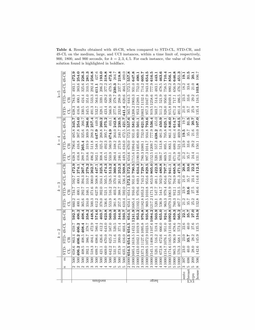
Table 4. Results obtained with 4S-CR, when compared to STD-CL, STD-CR, and4S-CL on the medium, large, and UCI instances, within a time limit of, respectively,900, 1800, and 900 seconds, for k = 2, 3, 4, 5. For each instance, the value of the bestsolution found is highlighted in boldface.

k=

2k

=3

k=

4k=

5

nm

ST

D-

ST

D-

4S-C

L4S-C

RST

D-

ST

D-4S-C

L4S-C

RST

D-

ST

D-4S-C

L4S-C

RST

D-

ST

D-4S-C

L4S-C

RC

LC

RC

LC

RC

LC

RC

LC

R

medium

2500

658.6

863.4

659.7

592.7

660.2

734.7

592.7

472.9

638.3

790.6

485.8

345.7

638.3

784.9

493.1

472.9

2500406.2

406.2

406.2

406.2

400.1

400.1

400.1

274.1

416.8

416.8

387.8

254.0

416.8

400.1

383.6

254.0

2500

408.5

408.5

408.4

408.4

365.6

292.7

394.3

267.4

288.7

265.4

325.6

266.7

330.5

424.4

325.6

226.3

3500

392.1

386.7

378.7

358.2

334.0

346.1

310.7

279.2

318.6

319.9

309.9

286.6

345.5

351.0

310.5

281.3

3500

518.3

484.1

472.9

448.5

500.3

371.6

300.0

262.7

496.2

511.8

288.2

257.4

491.3

533.3

292.4

256.8

3500

699.7

698.6

580.4

574.6

612.2

627.9

508.8

447.1

502.1

548.1

447.9

449.3

532.7

564.3

411.1

427.6

4500

421.1

426.6

412.2

403.7

378.0

392.0

334.1

325.3

308.4

325.2

268.8

260.2

328.1

339.1

206.2

193.0

4500

669.0

670.0

643.0

623.8

536.6

521.1

505.5

474.3

435.5

492.3

395.7

375.2

423.4

429.2

377.2

318.8

4500

642.2

625.2

587.0

569.3

553.9

516.2

528.5

513.2

550.9

580.9

474.9

493.1

566.9

566.9

479.5

472.4

5500

531.7

511.6

520.5

503.9

381.8

403.2

370.4

360.8

280.4

348.2

264.0

242.8

277.6

278.7

230.3

264.7

5500

373.9

399.0

371.4

344.9

257.3

388.7

261.0

252.3

246.1

273.9

240.7

230.5

232.0

298.9

237.7

218.8

5500

635.1

616.0

603.4

593.7

610.4

592.0

536.4

509.8

449.3

616.0

472.5

421.7

441.4

620.6

464.5

489.0

large

21000654.5

654.5

654.5

654.5

654.1

654.1

572.5

572.5

654.6

670.0

572.5

557.6

565.7

644.5

572.5

557.8

21000

1685.4

1618.5

1452.5

1241.9

1685.4

916.0

931.0

790.5

1715.6

1994.0

931.0

581.6

1208.2

1903.3

931.0

647.8

21000

1423.0

1042.1

1019.9

953.2

1102.5

970.6

849.1

634.3

1190.9

1405.6

809.0

501.1

953.2

1289.1

752.0

490.1

31000

1371.2

1127.6

1095.8

976.8

1182.8

1053.2

743.2

729.7

780.3

1089.1

732.0

621.9

1003.7

1132.4

714.2

605.7

31000

1099.5

1072.9

1023.5

935.8

969.5

1010.8

953.6

829.5

997.3

1014.7

934.8

793.6

957.3

1047.9

943.4

654.5

31000

1545.1

1408.3

1107.6

1084.2

1217.2

1171.3

853.9

805.0

1152.5

1209.7

777.9

536.4

919.5

1258.6

777.9

616.5

41000

520.1

516.2

519.4

503.9

520.1

547.7

481.1

422.3

520.1

557.3

438.2

455.0

503.7

514.3

483.1

443.1

41000

672.8

672.6

666.0

655.0

536.9

544.7

502.9

480.8

500.7

513.8

481.9

450.9

511.2

521.9

478.5

463.6

41000

1154.7

1076.1

951.0

924.1

963.3

979.4

854.6

797.7

869.5

895.1

705.8

625.1

928.0

950.6

758.5

710.4

51000

1174.6

1165.9

1110.6

1092.8

1079.3

1061.9

972.2

941.1

910.1

883.1

861.4

846.0

915.8

1049.4

880.2

856.1

51000

985.3

936.9

878.6

859.3

760.3

912.1

704.9

685.8

671.9

689.2

641.4

614.7

671.2

717.1

656.9

646.8

51000

570.3

568.1

573.2

565.2

487.7

531.5

491.3

471.5

474.0

521.2

469.9

464.5

481.4

486.5

476.2

451.3

UCIauto

3397

23.0

23.0

22.6

22.1

21.2

23.9

21.0

20.8

21.2

23.9

19.5

19.7

21.0

23.3

18.2

19.1

bre

ast

5698

40.0

35.7

40.0

35.7

35.7

33.6

35.7

33.6

35.7

33.6

35.7

31.5

35.7

33.6

33.6

31.5

cpu

5209

28.0

28.2

27.6

27.0

25.2

27.5

23.4

22.2

24.4

29.2

21.6

20.7

25.9

29.2

21.0

20.1

house

8506

142.6

145.9

135.5

134.9

132.8

146.6

114.6

112.4

131.1

150.1

110.0

107.0

135.4

134.5

103.8

106.7

found before and after carrying out the domain partition phase at the end of themethod, we register an increase in fitting error of up to 4 times for both STD-CRand STD-CL. This suggests the lack of a strong correlation, in both algorithms,between the quality of the solutions found before and after constructing the fi-nal domain partition. Also note that, with the adoption of our criterion for theidentification of critical points, the Point Partition step becomes more timeconsuming. Indeed, our experiments show that the average number of iterationscarried out in the time limit by STD-CR with respect to those for STD-CL canbe up to 40% smaller (as observed for the large instances with k = 5). There-fore, investing more computing time in a more refined criterion for the Point

Partition step turns out to be not effective for a method (such as STD-CR)which only considers the domain partition aspect in a second phase.

7 Concluding remarks

We have addressed the k-PAMF-PLS problem of fitting a piecewise affine modelwith a pairwise linearly separable domain partition to a set of data points.We have proposed an MILP formulation to solve the problem to optimality,strengthened via symmetry breaking constraints. To solve larger instances, wehave developed a four-step heuristic algorithm which simultaneously deals withthe various aspects of the problem. It is based on two key ideas: a criterion forthe identification of a set of critical points to be reassigned and the introductionof a domain partitioning step at each iteration of the method.

Computational experiments on a set of structured randomly generated andreal-world instances show that with our MILP formulation with symmetry break-ing constraints we can solve to optimality small-size instances, while our four-stepheuristic provides close-to-optimal solutions for small-size instances and allowsto tackle instances of much larger size. The results not only indicate the highquality of the solutions found by 4S-CR when compared to those obtained witheither an exact method or a standard two-phase heuristic algorithm, but theyalso highlight the relevance of the different features of 4S-CR, which must beadopted in a joint way to yield higher quality solutions to k-PAMF-PLS.

References

[AC13] E. Amaldi and S. Coniglio. A distance-based point-reassignment heuristicfor the k-hyperplane clustering problem. European Journal of OperationalResearch, 227(1):22–29, 2013.

[ACT11] E. Amaldi, S. Coniglio, and L. Taccari. Formulations and heuristics forthe k-piecewise affine model fitting problem. In Proc. of 10th Cologne-Twente Workshop on Graphs and Combinatorial Optimization (CTW),Frascati (Rome), Italy, pages 48–51, 2011.

[ACT12] E. Amaldi, S. Coniglio, and L. Taccari. k-Piecewise Affine Model Fitting:heuristics based on multiway linear classification. In Proc. of 11th Cologne-Twente Workshop on Graphs and Combinatorial Optimization (CTW),

Munich, Germany, pages 16–19. Universitat der Bundeswehr Munchen,2012.

[ADC13] E. Amaldi, K. Dhyani, and A. Ceselli. Column generation for the mini-mum hyperplanes clustering problem. INFORMS Journal on Computing,25(3):446–460, 2013.

[AM02] E. Amaldi and M. Mattavelli. The min pfs problem and piecewise linearmodel estimation. Discrete Applied Mathematics, 118(1-2):115–143, 2002.

[BGPV03] A. Bemporad, A. Garulli, S. Paoletti, and A. Vicino. A greedy approachto identification of piecewise affine models. In O. Maler and A. Pnueli, ed-itors, Hybrid Systems: Computation and Control, volume 2623 of LectureNotes in Computer Science, pages 97–112. Springer Berlin Heidelberg,2003.

[BM94] K. Bennet and O. Mangasarian. Multicategory discrimination via linearprogramming. Optimization Methods and Software, 3:27–39, 1994.

[BM00] P. Bradely and O. Mangasarian. k-plane clustering. Journal of GlobalOptimization, 16:23–32, 2000.

[BS07] D. Bertsimas and R. Shioda. Classification and regression via integeroptimization. Operations Research, 55:252–271, 2007.

[Con11] S. Coniglio. The impact of the norm on the k-Hyperplane Clusteringproblem: relaxations, restrictions, approximation factors, and exact for-mulations. In Proc. of 10th Cologne-Twente Workshop on Graphs andCombinatorial Optimization (CTW), Frascati (Rome), Italy, pages 118–121, 2011.

[Con15] S. Coniglio. On the optimization of vector norms and the k-hyperplaneclustering problem: tightened exact and approximated formulations withinan approximation factor. Technical report, Lehrstuhl II fur Mathematik,RWTH Aachen University, 2015.

[DF66] R. Duda and H. Fossum. Pattern classification by iteratively determinedlinear and piecewise linear discriminant functions. IEEE Transactions onElectronic Computers, 15:220–232, 1966.

[FA13] A. Frank and A. Asuncion. UCI machine learning repository, 2013. http://archive.ics.uci.edu/ml.

[FTMLM03] G. Ferrari-Trecate, M. Muselli, D. Liberati, and M. Morari. A clusteringtechnique for the identification of piecewise affine systems. Automatica,39(2):205–217, 2003.

[KP08] V. Kaibel and M. E. Pfetsch. Packing and partitioning orbitopes. Math-ematical Programming, Series A, 114:1–36, 2008.

[Mac67] J. MacQueen. Some methods for classification and analysis of multivariateobservations. In Proc. of 5th Berkeley Symposium on Mathematical Statis-tistics and Probability, Los Angeles, California, volume 1, pages 281–297.California University Press, 1967.

[Mar10] F. Margot. Symmetry in integer linear programming. In M. Junger,T. Liebling, D. Naddef, G. Nemhauser, W. Pulleyblank, G. Reinelt, G. Ri-naldi, and L. Wolsey, editors, 50 Years of Integer Programming 1958-2008,pages 647–686. Springer Berlin Heidelberg, 2010.

[MB09] A. Magnani and S. Boyd. Convex piecewise-linear fitting. Optimizationand Engineering, 10:1–17, 2009.

[MDZ01] I. Mendez-Dıaz and P. Zabala. A polyhedral approach for graph coloring.Electronic Notes in Discrete Mathematics, 7:178–181, 2001.

[MDZ06] I. Mendez-Dıaz and P. Zabala. A branch-and-cut algorithm for graphcoloring. Discrete Applied Mathematics, 154(5):826–847, 2006.

[MRT05] O. Mangasarian, J. Rosen, and M. Thompson. Global minimizationvia piecewise-linear underestimation. Journal of Global Optimization,32(1):1–9, 2005.

[RBL04] J. Roll, A. Bemporad, and L. Ljung. Identification of piecewise affinesystems via mixed-integer programming. Automatica, 40:37–50, 2004.

[TPSM06] M. Tabatabaei-Pour, K. Salahshoor, and B. Moshiri. A modified k-planeclustering algorithm for identification of hybrid systems. In Proc. of 6thWorld Congress on Intelligent Control and Automation (WCICA), vol-ume 1, pages 1333–1337. IEEE, 2006.

[TV12] A. Toriello and J.P. Vielma. Fitting piecewise linear continuous functions.European Journal of Operational Research, 219(1):86–95, 2012.

[Vap96] V. Vapnik. The Nature of Statistical Learning Theory. Springer, 1996.