Discrete Structures (2IT50)

Rob Hoogerwoord & Hans Zantema

August, 2016

1

2

Contents

0.1 Introduction . . . . . . . . . . . . . . . . . . . . . . . . . . . . . . . . . 50.2 Basic set theory . . . . . . . . . . . . . . . . . . . . . . . . . . . . . . . 50.3 The principle of induction . . . . . . . . . . . . . . . . . . . . . . . . . 6

1 Relations 81.1 Binary relations . . . . . . . . . . . . . . . . . . . . . . . . . . . . . . . 81.2 Equivalence relations . . . . . . . . . . . . . . . . . . . . . . . . . . . . 121.3 Operations on Relations . . . . . . . . . . . . . . . . . . . . . . . . . . 16

1.3.1 Set operations . . . . . . . . . . . . . . . . . . . . . . . . . . . 171.3.2 Transposition . . . . . . . . . . . . . . . . . . . . . . . . . . . . 171.3.3 Composition . . . . . . . . . . . . . . . . . . . . . . . . . . . . 181.3.4 Closures . . . . . . . . . . . . . . . . . . . . . . . . . . . . . . . 22

1.4 Exercises . . . . . . . . . . . . . . . . . . . . . . . . . . . . . . . . . . 24

2 Graphs 302.1 Directed Graphs . . . . . . . . . . . . . . . . . . . . . . . . . . . . . . 302.2 Undirected Graphs . . . . . . . . . . . . . . . . . . . . . . . . . . . . . 312.3 A more compact notation for undirected graphs . . . . . . . . . . . . . 332.4 Additional notions and some properties . . . . . . . . . . . . . . . . . 332.5 Connectivity . . . . . . . . . . . . . . . . . . . . . . . . . . . . . . . . 35

2.5.1 Paths . . . . . . . . . . . . . . . . . . . . . . . . . . . . . . . . 352.5.2 Path concatenation . . . . . . . . . . . . . . . . . . . . . . . . . 372.5.3 The triangular inequality . . . . . . . . . . . . . . . . . . . . . 382.5.4 Connected components . . . . . . . . . . . . . . . . . . . . . . 39

2.6 Cycles . . . . . . . . . . . . . . . . . . . . . . . . . . . . . . . . . . . . 402.6.1 Directed cycles . . . . . . . . . . . . . . . . . . . . . . . . . . . 402.6.2 Undirected cycles . . . . . . . . . . . . . . . . . . . . . . . . . . 41

2.7 Euler and Hamilton cycles . . . . . . . . . . . . . . . . . . . . . . . . . 422.7.1 Euler cycles . . . . . . . . . . . . . . . . . . . . . . . . . . . . . 422.7.2 Hamilton cycles . . . . . . . . . . . . . . . . . . . . . . . . . . . 442.7.3 A theorem on Hamilton cycles . . . . . . . . . . . . . . . . . . 442.7.4 A proof by contradiction . . . . . . . . . . . . . . . . . . . . . . 452.7.5 A more explicit proof . . . . . . . . . . . . . . . . . . . . . . . 462.7.6 Proof of the Core Property . . . . . . . . . . . . . . . . . . . . 46

2.8 Ramsey’s theorem . . . . . . . . . . . . . . . . . . . . . . . . . . . . . 492.8.1 Introduction . . . . . . . . . . . . . . . . . . . . . . . . . . . . 492.8.2 Ramsey’s theorem . . . . . . . . . . . . . . . . . . . . . . . . . 502.8.3 A few applications . . . . . . . . . . . . . . . . . . . . . . . . . 53

2.9 Trees . . . . . . . . . . . . . . . . . . . . . . . . . . . . . . . . . . . . . 542.9.1 Undirected trees . . . . . . . . . . . . . . . . . . . . . . . . . . 54

2.10 Exercises . . . . . . . . . . . . . . . . . . . . . . . . . . . . . . . . . . 55

3

3 Functions 593.1 Functions . . . . . . . . . . . . . . . . . . . . . . . . . . . . . . . . . . 593.2 Equality of functions . . . . . . . . . . . . . . . . . . . . . . . . . . . . 603.3 Monotonicity of function types . . . . . . . . . . . . . . . . . . . . . . 603.4 Function composition . . . . . . . . . . . . . . . . . . . . . . . . . . . 613.5 Lifting a function . . . . . . . . . . . . . . . . . . . . . . . . . . . . . . 613.6 Surjective, injective, and bijective functions . . . . . . . . . . . . . . . 643.7 Inverse functions . . . . . . . . . . . . . . . . . . . . . . . . . . . . . . 663.8 Finite sets and counting . . . . . . . . . . . . . . . . . . . . . . . . . . 683.9 Exercises . . . . . . . . . . . . . . . . . . . . . . . . . . . . . . . . . . 72

4 Posets and lattices 744.1 Partial orders . . . . . . . . . . . . . . . . . . . . . . . . . . . . . . . . 744.2 Extreme elements . . . . . . . . . . . . . . . . . . . . . . . . . . . . . . 774.3 Upper and lower bounds . . . . . . . . . . . . . . . . . . . . . . . . . . 804.4 Lattices . . . . . . . . . . . . . . . . . . . . . . . . . . . . . . . . . . . 84

4.4.1 Definition . . . . . . . . . . . . . . . . . . . . . . . . . . . . . . 844.4.2 Algebraic properties . . . . . . . . . . . . . . . . . . . . . . . . 854.4.3 Distributive lattices . . . . . . . . . . . . . . . . . . . . . . . . 874.4.4 Complete lattices . . . . . . . . . . . . . . . . . . . . . . . . . . 88

4.5 Exercises . . . . . . . . . . . . . . . . . . . . . . . . . . . . . . . . . . 90

5 Monoids and Groups 935.1 Operators and their properties . . . . . . . . . . . . . . . . . . . . . . 935.2 Semigroups and monoids . . . . . . . . . . . . . . . . . . . . . . . . . . 955.3 Groups . . . . . . . . . . . . . . . . . . . . . . . . . . . . . . . . . . . . 975.4 Subgroups . . . . . . . . . . . . . . . . . . . . . . . . . . . . . . . . . . 1015.5 Cosets and Lagrange’s Theorem . . . . . . . . . . . . . . . . . . . . . . 1025.6 Permutation Groups . . . . . . . . . . . . . . . . . . . . . . . . . . . . 104

5.6.1 Function restriction and extension . . . . . . . . . . . . . . . . 1045.6.2 Continued Compositions . . . . . . . . . . . . . . . . . . . . . . 1055.6.3 Bijections . . . . . . . . . . . . . . . . . . . . . . . . . . . . . . 1055.6.4 Permutations . . . . . . . . . . . . . . . . . . . . . . . . . . . . 1065.6.5 Swaps . . . . . . . . . . . . . . . . . . . . . . . . . . . . . . . . 1075.6.6 Neighbor swaps . . . . . . . . . . . . . . . . . . . . . . . . . . . 109

5.7 Exercises . . . . . . . . . . . . . . . . . . . . . . . . . . . . . . . . . . 111

6 Combinatorics: the Art of Counting 1146.1 Introduction . . . . . . . . . . . . . . . . . . . . . . . . . . . . . . . . . 1146.2 Recurrence Relations . . . . . . . . . . . . . . . . . . . . . . . . . . . . 121

6.2.1 An example . . . . . . . . . . . . . . . . . . . . . . . . . . . . . 1216.2.2 The characteristic equation . . . . . . . . . . . . . . . . . . . . 1226.2.3 Linear recurrence relations . . . . . . . . . . . . . . . . . . . . 1246.2.4 Summary . . . . . . . . . . . . . . . . . . . . . . . . . . . . . . 127

6.3 Binomial Coefficients . . . . . . . . . . . . . . . . . . . . . . . . . . . . 127

4

6.3.1 Factorials . . . . . . . . . . . . . . . . . . . . . . . . . . . . . . 1276.3.2 Binomial coefficients . . . . . . . . . . . . . . . . . . . . . . . . 1296.3.3 The Shepherd’s Principle . . . . . . . . . . . . . . . . . . . . . 1306.3.4 Newton’s binomial formula . . . . . . . . . . . . . . . . . . . . 131

6.4 A few examples . . . . . . . . . . . . . . . . . . . . . . . . . . . . . . . 1326.4.1 Summary . . . . . . . . . . . . . . . . . . . . . . . . . . . . . . 134

6.5 Exercises . . . . . . . . . . . . . . . . . . . . . . . . . . . . . . . . . . 135

7 Number Theory 1387.1 Introduction . . . . . . . . . . . . . . . . . . . . . . . . . . . . . . . . . 1387.2 Divisibility . . . . . . . . . . . . . . . . . . . . . . . . . . . . . . . . . 1387.3 Greatest common divisors . . . . . . . . . . . . . . . . . . . . . . . . . 1417.4 Euclid’s algorithm and its extension . . . . . . . . . . . . . . . . . . . 1457.5 The prime numbers . . . . . . . . . . . . . . . . . . . . . . . . . . . . . 1487.6 Modular Arithmetic . . . . . . . . . . . . . . . . . . . . . . . . . . . . 152

7.6.1 Congruence relations . . . . . . . . . . . . . . . . . . . . . . . . 1527.6.2 An application: the nine and eleven tests . . . . . . . . . . . . 155

7.7 Fermat’s little theorem . . . . . . . . . . . . . . . . . . . . . . . . . . . 1567.8 Cryptography: the RSA algorithm . . . . . . . . . . . . . . . . . . . . 1577.9 Exercises . . . . . . . . . . . . . . . . . . . . . . . . . . . . . . . . . . 159

5

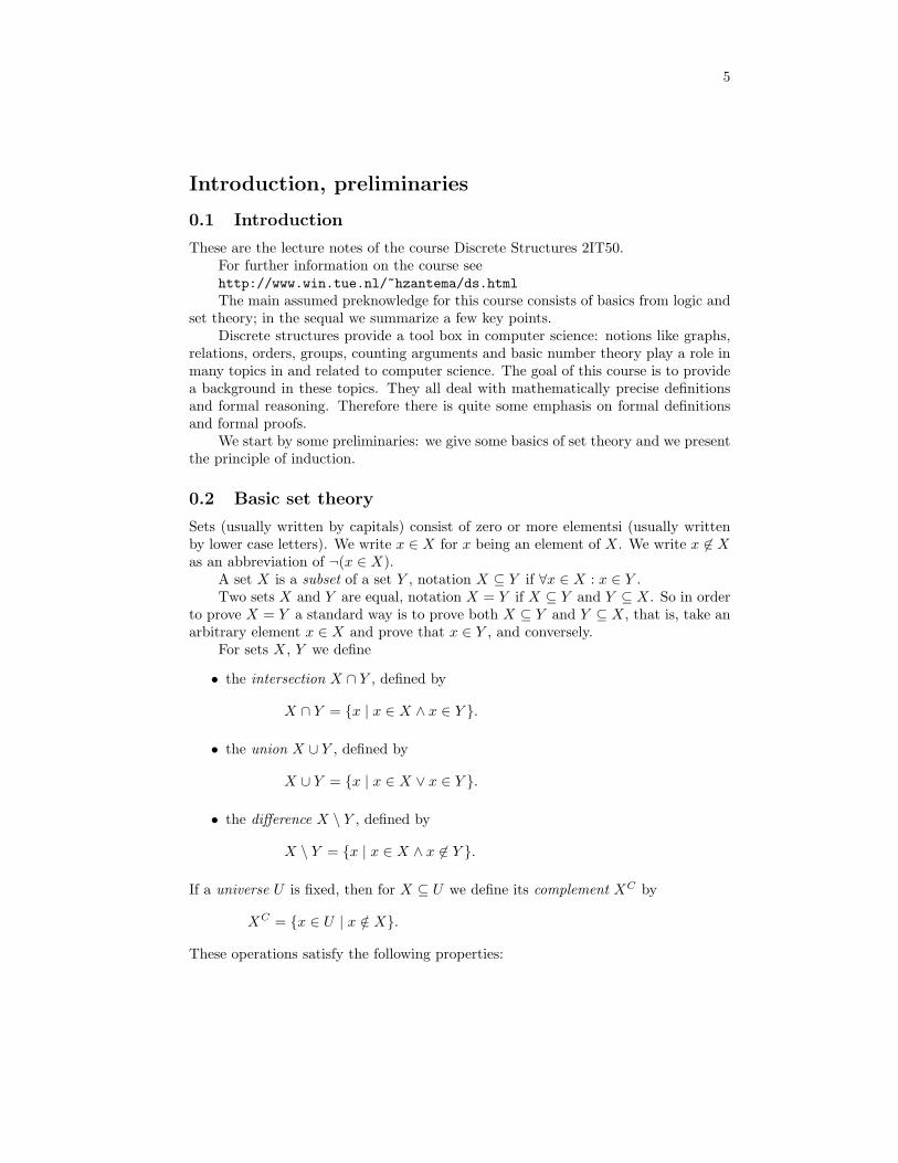
Introduction, preliminaries

0.1 Introduction

These are the lecture notes of the course Discrete Structures 2IT50.For further information on the course seehttp://www.win.tue.nl/~hzantema/ds.htmlThe main assumed preknowledge for this course consists of basics from logic and

set theory; in the sequal we summarize a few key points.Discrete structures provide a tool box in computer science: notions like graphs,

relations, orders, groups, counting arguments and basic number theory play a role inmany topics in and related to computer science. The goal of this course is to providea background in these topics. They all deal with mathematically precise definitionsand formal reasoning. Therefore there is quite some emphasis on formal definitionsand formal proofs.

We start by some preliminaries: we give some basics of set theory and we presentthe principle of induction.

0.2 Basic set theory

Sets (usually written by capitals) consist of zero or more elementsi (usually writtenby lower case letters). We write x ∈ X for x being an element of X. We write x 6∈ Xas an abbreviation of ¬(x ∈ X).

A set X is a subset of a set Y , notation X ⊆ Y if ∀x ∈ X : x ∈ Y .Two sets X and Y are equal, notation X = Y if X ⊆ Y and Y ⊆ X. So in order

to prove X = Y a standard way is to prove both X ⊆ Y and Y ⊆ X, that is, take anarbitrary element x ∈ X and prove that x ∈ Y , and conversely.

For sets X, Y we define

• the intersection X ∩ Y , defined by

X ∩ Y = x | x ∈ X ∧ x ∈ Y .

• the union X ∪ Y , defined by

X ∪ Y = x | x ∈ X ∨ x ∈ Y .

• the difference X \ Y , defined by

X \ Y = x | x ∈ X ∧ x 6∈ Y .

If a universe U is fixed, then for X ⊆ U we define its complement XC by

XC = x ∈ U | x /∈ X.

These operations satisfy the following properties:

6

• Idempotence: X ∩X = X, X ∪X = X.

• Commutativity: X ∩ Y = Y ∩X, X ∪ Y = Y ∪X.

• Associativity: (X ∩ Y ) ∩ Z = X ∩ (Y ∩ Z), (X ∪ Y ) ∪ Z = X ∪ (Y ∪ Z).

• Distributivity: X∪(Y ∩Z) = (X∪Y )∩(X∪Z), X∩(Y ∪Z) = (X∩Y )∪(X∩Z).

• DeMorgan’s Laws: (X ∪ Y )C = XC ∩ Y C , (X ∩ Y )C = XC ∪ Y C .

These rules satisfy the principle of duality: if in a valid rule every symbol ∪ is replacedby ∩ and conversely, then a valid rule is obtained.

The operations presented until now all result in subsets of the same universe.This does not hold for the following two operations:

• The Cartesian product

X × Y = (x, y) | x ∈ X ∧ y ∈ Y .

• The Power set

P(X) = 2X = Y | Y ⊆ X.

0.3 The principle of induction

In proving properties we often use the principle of induction. In its basic version itstates:

Let P be a property depending on natural numbers, for which P (0) holds,and for every n we can conclude P (n+ 1) from the induction hypothesisP (n). Then P (n) holds for every natural number n.

A fruitful variant, sometimes called strong induction is the following:

Let P be a property depending on natural numbers, for which for every nwe can conclude P (n) from the induction hypothesis ∀k < n : P (k). ThenP (n) holds for every natural number n.

Here k, n run over the natural numbers.So the difference is as follows. In the basic version we prove P (n + 1) from the

assumption that P (n) holds, that is, for n being the direct predecessor of the valuen+ 1 for which we want to prove the property. In contrast, in the strong version wetry to prove P (n), assuming that P (k) holds for all predecessors k of n, not only thedirect predecessor.

Surprisingly, we can prove validity of the strong version by only using the basicversion, as follows.

Assume that we can conclude P (n) from the (strong) induction hypothesis ∀k <n : P (k). We have to prove that P (n) holds for every natural number n. We dothis by proving that Q(n) ≡ ∀k < n : P (k) holds for every n, by (the basic version

7

of) induction on n. First we observe that Q(0) holds, which is trivially true since nonatural number k < 0 exists. Next we assume the (basic) induction hypothesis Q(n)and try to prove Q(n + 1) ≡ ∀k < n + 1 : P (k). So let k < n + 1. If k < n then weconclude P (k) by the (basic) induction hypothesis Q(n). If not, then k = n, and byour start assumption we obtain P (n). So we conclude Q(n+ 1) ≡ ∀k < n+ 1 : P (k).So by the basic version of induction we conclude that Q(n) holds for every n. But wehad to conclude that P (n) holds for every n. So let n be arbitrary. Since n < n + 1and we know that Q(n+1) holds, we conclude that P (n) holds, concluding the proof.

8

1 Relations

1.1 Binary relations

A (binary) relation R from set U to set V is a subset of the Cartesian productU×V . If (u, v)∈R , we say that u is in relation R to v . We usually denote this byuRv . Set U is called the domain of the relation and V its range (or: codomain).If U =V we call R an (endo)relation on U .

1.1 Examples.

(a) “Is the mother of” is a relation from the set of all women to the set of all people.It consists of all pairs ( person1 , person2 ) where person1 is the mother ofperson2 . Of course, this relation also is an (endo)relation on the set of people.

(b) “There is a train connection between” is a relation on the set of cities in theNetherlands.

(c) The equality relation “ = ” is a relation on every set. This relation is oftendenoted by I (and also called the “identity” relation). Because, however, everyset has its “own” identity relation we sometimes use subscription to distinguishall these different identity relations. That is, for every set U we define IU by:

IU = (u, u) | u∈U .

Whenever no confusion is possible and it is clear which set is intended, we dropthe subscript and write just I instead of IU , and in ordinary mathematicallanguage we use “ = ”, as always. So, for any set U and for all u, v∈U , wehave: uI v ⇔ u= v .

(d) Integer n divides integer m , notation n|m , if there is an integer q∈Z such thatq∗n=m . Divides | is the relation on Z that consists of all pairs (n,m) ∈ Z× Zwith (∃q : q∈Z : q∗n=m ) .

(e) “Less than” ( < ) and “greater than” ( > ) are relations on R, and on Q,Z, andN as well, and so are “at most” ( ≤ ) and “at least” ( ≥ ).

(f) The set (a, p) , (b, p) , (b, q) , (c, q) is a relation from a, b, c to p, q .

(g) The set (x, y) ∈ R2 | y = x2 is a relation on R.

(h) Let Ω be a set, then “is a subset of” ( ⊆ ) is a relation on the set of all subsetsof Ω .

Besides binary relations we can also consider n -ary relations for any n≥ 0 . An n -aryrelation on sets U0, · · · , Un−1 is a subset of the Cartesian product U0 × · · · × Un−1 .Unless stated otherwise, in this text relations are binary.

Let R be a relation from set U to set V . Then for each element u∈U we define[u ]R as a subset of V , as follows:

9

[u ]R = v∈V | uRv .

(Sometimes [u ]R is also denoted by R(u) .) This set is called the (R -)image of u .Similarly, for v∈V a subset of U called R[v ] is defined by:

R[v ] = u∈U | uRv ,

which is called the (R -)pre-image of v .

1.2 Definition. If R is a relation from finite set U to finite set V , then R can berepresented by means of a so-called adjacency matrix ; sometimes this is convenientbecause it allows computations with (finite) relations to be carried out in terms ofmatrix calculations. We will see examples of this later.

With m for the size – the number of elements – of U and with n for the sizeof V , sets U and V can be represented by finite sequences, by numbering theirelements. That is, we assume U = u1, · · · , um and we assume V = v1, · · · , vn .The adjacency matrix of relation R then is an m×n matrix AR , say, the elementsof which are 0 or 1 only, and defined by, for all i, j : 1≤i≤m ∧ 1≤j≤n :

AR[ i, j ] = 1 ⇔ uiR vj .

Here AR[ i, j ] denotes the element of matrix AR at row i and column j . Note thatthis definition is equivalent to stating that AR[ i, j ] = 0 if and only if ¬(uiR vj ) , forall i, j . Actually, adjacency matrices are boolean matrices in which, for the sake ofconciseness, true is encoded as 1 and false as 0 ; thus, we might as well state that:AR[ i, j ] ⇔ uiR vj .2

Notice that this representation is not unique: the elements of finite sets can be as-signed numbers in very many ways, and the distribution of 0 ’s and 1 ’s over thematrix depends crucially on how the elements of the two sets are numbered. Forinstance, if U has m elements it can be represented by m! different sequences oflength m ; thus, a relation between sets of sizes m and n admits as many as m! ∗ n!(potentially different) adjacency matrices for its representation. Not surprisingly, ifU =V it is good practice to use one and the same element numbering for the two U ’s(in U×U ). If 1≤i≤m then the set [ui ]R is represented by the row with index i inthe adjacency matrix, that is:

[ui ]R = vj | 1≤j≤n ∧ AR[ i, j ] = 1 .

Similarly, for 1≤j≤n we have:

R[vj ] = ui | 1≤i≤m ∧ AR[ i, j ] = 1 .

1.3 Examples.

(a) An adjacency matrix for the relation (a, p) , (b, p) , (b, q) , (c, q) from a, b, cto p, q is:

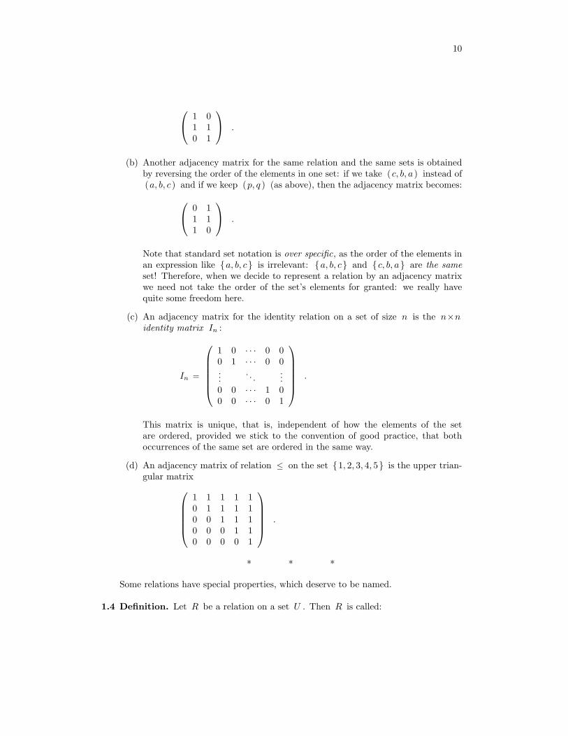
10

1 01 10 1

.

(b) Another adjacency matrix for the same relation and the same sets is obtainedby reversing the order of the elements in one set: if we take (c, b, a ) instead of(a, b, c ) and if we keep (p, q ) (as above), then the adjacency matrix becomes: 0 1

1 11 0

.

Note that standard set notation is over specific, as the order of the elements inan expression like a, b, c is irrelevant: a, b, c and c, b, a are the sameset! Therefore, when we decide to represent a relation by an adjacency matrixwe need not take the order of the set’s elements for granted: we really havequite some freedom here.

(c) An adjacency matrix for the identity relation on a set of size n is the n×nidentity matrix In :

In =

1 0 · · · 0 00 1 · · · 0 0...

. . ....

0 0 · · · 1 00 0 · · · 0 1

.

This matrix is unique, that is, independent of how the elements of the setare ordered, provided we stick to the convention of good practice, that bothoccurrences of the same set are ordered in the same way.

(d) An adjacency matrix of relation ≤ on the set 1, 2, 3, 4, 5 is the upper trian-gular matrix

1 1 1 1 10 1 1 1 10 0 1 1 10 0 0 1 10 0 0 0 1

.

* * *

Some relations have special properties, which deserve to be named.

1.4 Definition. Let R be a relation on a set U . Then R is called:

11

• reflexive, if for all x∈U we have: xRx ;

• irreflexive, if for all x∈U we have: ¬(xRx) ;

• symmetric, if for all x, y∈U we have: xRy ⇔ yRx ;

• antisymmetric, if for all x, y∈U we have: xRy ∧ yRx ⇒ x= y ;

• transitive, if for all x, y, z∈U we have: xRy ∧ yRz ⇒ xRz .

1.5 Examples. We consider some of the examples given earlier:

(a) “Is the mother of” is a relation on the set of all people. It is irreflexive, anti-symmetric, and not transitive.

(b) “There is a train connection between” is symmetric and transitive. If one iswilling to accept traveling over a zero distance as a train connection, then thisrelation also is reflexive.

(c) On every set relation “equals” ( = ) is reflexive, symmetric, and transitive.

(d) Relation “divides” ( | ) is reflexive, antisymmetric, and transitive.

(e) “Less than” ( < ) and “greater than” ( > ) on R are irreflexive, antisymmet-ric, and transitive, whereas “at most” ( ≤ ) and “at least” ( ≥ ) are reflexive,antisymmetric, and transitive.

(f) The relation (x, y)∈R2 | y = x2 is neither reflexive nor irreflexive.

2

For any relation R the proposition (∀x, y : x, y∈U : xRy ⇔ yRx ) is (logically)equivalent to the proposition (∀x, y : x, y∈U : xRy ⇒ yRx ) , which is (formally)weaker. Hence, relation R is symmetric if xRy ⇒ yRx , for all x, y∈U . To provethat R is symmetric, therefore, it suffices to prove the latter, weaker, version of theproposition, whereas to use (in other proofs) that R is symmetric we may use thestronger version.

1.6 Lemma. Every reflexive relation R on set U satisfies: u∈ [u ]R , for all u∈U .

Proof. By calculation:

u∈ [u ]R⇔ definition of [u ]R

uRu

⇔ R is reflexive true

12

1.7 Lemma. Every symmetric relation R on set U satisfies: v ∈ [u ]R ⇔ u∈ [v ]R , forall u, v∈U .

Proof. By calculation:

v ∈ [u ]R⇔ definition of [u ]R

uRv

⇔ R is symmetric v Ru

⇔ definition of [v ]R u∈ [v ]R

* * *

If R is a relation on a finite set S , then special properties like reflexivity, symmetryand transitivity can be read off from the adjacency matrix. For example, R is reflexiveif and only if the main diagonal of R ’s adjacency matrix contains 1 ’s only, that is ifAR[ i, i ] = 1 for all (relevant) i .

Relation R is symmetric if and only if the transposed matrix ATR equals AR .

The transposed matrix MT of an m×n matrix M is the n×m matrix defined by,for all i, j :

MT[j, i ] = M [ i, j ] .

1.2 Equivalence relations

Relations that are reflexive, symmetric, and transitive deserve some special attention:they are called equivalence relations.

1.8 Definition. A relation R is an equivalence relation if and only if it is reflexive,symmetric, and transitive.2

If elements u and v are related by an equivalence relation R , that is, if uRv , thenu and v are also called “equivalent (under R )”.

1.9 Example. On every set relation “equals” ( = ) is an equivalence relation.

1.10 Example. Consider the plane R2 and in it the set S of straight lines. We call twolines in S parallel if and only if they are equal or do not intersect. Hence, two linesin S are parallel if and only if their slopes are equal. Being parallel is an equivalencerelation on the set S .

13

1.11 Example. We consider a fixed d∈Z , d> 0 , and we define a relation R on Zby: mRn if and only if m−n is divisible by d . The latter can be formulatedas (m−n) modd = 0 , and a more traditional mathematical rendering of this ism=n (mod d) . Thus defined, R is an equivalence relation.2

Actually, the last two examples are instances of Theorem 1.13. Before giving thistheorem, first we introduce equivalence classes and prove a lemma about them.If R is an equivalence relation on set U , then, for every u∈U the set [u ]R is calledthe equivalence class of u . Because equivalence relations are reflexive we have, as wehave seen in lemma 1.6 : u∈[u ]R , for all u∈U . From this it follows immediately thatequivalence classes are nonempty. Equivalence classes have several other interestingproperties. For example, the equivalence classes of two elements are equal if and onlyif these elements are equivalent:

1.12 Lemma. Every equivalence relation R on set U satisfies, for all u, v∈U :

[u ]R = [v ]R ⇔ uR v .

Proof. The left-hand side of this equivalence contains the function [ · ]R , whereas theright-hand side does not. To eliminate [ · ]R we rewrite the left-hand side first:

[u ]R = [v ]R⇔ set equality

(∀x : x∈U : x∈[u ]R ⇔ x∈[v ]R )

⇔ definition of [ · ]R (∀x : x∈U : uRx ⇔ vRx ) ,

hence, the lemma is equivalent to:

(∀x : x∈U : uRx ⇔ vRx ) ⇔ uR v .

This we prove by mutual implication.

“⇒ ”: (∀x : x∈U : uRx ⇔ vRx )

⇒ instantiation x := v uRv ⇔ vRv

⇔ R is an equivalence relation, so it is reflexive uR v .

“⇐ ”: Assuming uRv and for any x∈U we prove uRx ⇔ vRx , again by mutualimplication:

uR x

⇔ assumption

14

uR v ∧ uR x

⇔ R is an equivalence relation, so it is symmetric v R u ∧ uR x

⇒ R is an equivalence relation, so it is transitive v R x ,

and:

v R x

⇔ assumption uR v ∧ v R x

⇒ R is an equivalence relation, so it is transitive uR x ,

which concludes the proof of this lemma.

1.13 Theorem. A relation R on a set U is an equivalence relation if and only if a set Vand a function f : U → V exists such that

xR y ⇔ f(x) = f(y)

for all x, y∈U .

Proof.First we prove the ’if’-part: assume such a V and f exists; we have to prove that

R is an equivalence relation.Choose x ∈ U arbitrary, then xRx holds since f(x) = f(x). So R is reflexive.Choose x, y ∈ U arbitrary for which then xRy holds. Then f(x) = f(y), so also

f(y) = f(x), so yRx holds. So R is symmetric.Choose x, y, z ∈ U arbitrary for which xRy and yRz holds. Then f(x) = f(y)

and f(y) = f(z), so also f(x) = f(z). Hence xRz holds. This proves that R istransitive.

Combining these three properties we conclude that R is an equivalence relation,concluding the ’if’-part.

Next we prove the ’only if’-part: assume R is an equivalence relation; we haveto find V and f having the required property.

Choose V to be the set of all subsets of U and define f(x) = [x ]R for all x ∈ U .Then the required property

xR y ⇔ f(x) = f(y)

holds due to Lemma 1.12.

15

1.14 Example. We reconsider Example 1.11. The predicate (m−n) modd = 0 is equiv-alent to mmodd = nmodd , so with Z both for set U and for set V , function f ,defined by f(m) = mmodd , for all m∈Z , does the job.2

As a further investigation of equivalence classes we now observe that they are eitherdisjoint or equal:

1.15 Lemma. Every equivalence relation R on set U satisfies, for all u, v∈U :

[u ]R ∩ [v ]R = ø ∨ [u ]R = [v ]R .

Proof. This proposition is equivalent to:

[u ]R ∩ [v ]R 6= ø ⇒ [u ]R = [v ]R ,

which we prove as follows:[u ]R ∩ [v ]R 6= ø

⇔ definition of ø and ∩ (∃x : x∈U : x∈[u ]R ∧x∈[v ]R )

⇔ definition of [ · ]R (∃x : x∈U : uRx∧ vRx )

⇒ R is symmetric and transitive (∃x : x∈U : uRv )

⇒ predicate calculus uR v

⇔ lemma 1.12 [u ]R = [v ]R

The equivalence classes of an equivalence relation “cover” the set:

1.16 Lemma. Every equivalence relation R on set U satisfies: (⋃

u:u∈U [u ]R) = U .

Proof. By mutual set inclusion. On the one hand, every equivalence class is a subsetof U , that is: [u ]R ⊆ U , for all u∈U ; hence, their union, (

⋃u:u∈U [u ]R) , is a

subset of U as well. On the other hand, we have for every v∈U that v∈[v ]R , so,

also v ∈ (⋃

u:u∈U [u ]R ) . Hence, U is a subset of (⋃

u:u∈U [u ]R ) too.

These lemmas show that the equivalence classes of an equivalence relation form a,so-called, partition of set U .

1.17 Definition. A partition of set U is a set Π of nonempty and disjoint subsets of U ,the union of which equals U . Formally, that set Π is a partition of U means theconjunction of:

16

(a) (∀X : X∈Π : X⊆U ∧ X 6= ø )

(b) (∀X,Y : X,Y ∈Π : X∩Y = ø ∨ X =Y )

(c) (⋃

X:X∈ΠX ) = U

2

Clause (a) in this definition expresses that the elements of a partition of U arenonempty subsets of U , clause (b) expresses that the sets in a partition are disjoint,whereas clause (c) expresses that the sets in a partition together “cover the whole”U . Phrased differently, clause (b) and (c) together express that every element of Uis an element of exactly one of the sets in the partition.

Conversely, every partition also represents an equivalence relation. Every elementof set U is element of exactly one of the subsets in the partition. “Being in the samesubset” (in the partition) is an equivalence relation.

1.18 Theorem. Every partition Π of a set U represents an equivalence relation on U ,the equivalence classes of which are the sets in Π .Proof. Because Π is a partition, every element of U is an element of a unique subsetin Π . Now, the relation “being elements of the same subset in Π ” is an equivalencerelation. Formally, we prove this by defining a function ϕ : U→Π , as follows, for allu∈U and X∈Π :

ϕ(u) =X ⇔ u∈X .

Thus defined, ϕ is a function indeed, because for every u∈U one and only one X∈Πexists satisfying u∈X . Now relation ∼ on U , defined by, for all u, v∈U :

u∼ v ⇔ ϕ(u) = ϕ(v) ,

is an equivalence relation – Theorem 1.13 ! – . Furthermore, by its very constructionϕ satisfies u∈ϕ(u) and, hence, ϕ(u) is the equivalence class of u , for all u∈U .

1.3 Operations on Relations

Relations between two sets are subsets of the Cartesian Product of these two sets.Hence, all usual set operations can be applied to relations as well. In addition, rela-tions admit of some dedicated operations that happen to have nice algebraic proper-ties. It is even possible to develop a viable Relational Calculus, but this falls outsidethe scope of this text.

These relational operations play an important role in the mathematical study ofprogramming constructs, such as recursion and data structures. They are also usefulin some theorems about graphs. We will see applications of this later.

17

1.3.1 Set operations

• For sets U and V , the extreme relations from U to V are the empty relation øand the full relation U×V . For the sake of brevity and symmetry, we denotethese two relations by ⊥ (“bottom”) and > (“top”) , respectively; elementwise, they satisfy, for all u∈U and v∈V :

¬(u⊥v) ∧ u>v .

For example, every relation R satisfies: ⊥⊆R and R⊆> , which is why wecall ⊥ and > the extreme relations.

• If R and S are relations, with the same domain and and with the same range,then R∪S , and R∩S , and R \S are relations too, between the same sets asR and S , and with the obvious meaning. The complement RC of relation Ris >\R .

• These operations have their usual algebraic properties. In particular, > and ⊥are the identity elements of ∪ and ∩ , respectively: R ∪⊥ = R and R ∩> = R .They are zero elements as well, that is: R ∪> = > and R ∩⊥ = ⊥ .

1.3.2 Transposition

With every relation R from set U to set V a corresponding relation exists fromV to U that contains (v, u) if and only if (u, v)∈R . This relation is called thetransposition of R and is denoted by RT . (Some mathematicians use R−1 , butthis may be confusing: transposition is not the same as inversion, especially withfunctions.) Formally, transposition is defined as follows.

1.19 Definition. For every relation R from set U to set V , relation RT from V to Uis defined by, for all v∈V and u∈U :

v RTu ⇔ uRv .

1.20 Lemma. Transposition distributes over all set operations, that is:

⊥T = ⊥ and: >T = > ;(R ∪ S)T = RT ∪ ST ;(R ∩ S)T = RT ∩ ST ;(R \ S)T = RT \ ST ;(RC)T = (RT)C .

1.21 Lemma. Transposition is its own inverse, that is, every relation R satisfies:

(RT)T = R .

2

18

For finite relations there is a direct connection between relation transposition andmatrix transposition:

1.22 Lemma. If AR is an adjacency matrix for relation R then (AR)T is an adjacencymatrix for RT .

1.23 Examples. Properties of relations, like (ir)reflexivity and (anti)symmetry, can nowbe expressed concisely by means of relational operations; for R a relation on set U :

• “R is reflexive ” ⇔ IU ⊆ R

• “R is irreflexive ” ⇔ IU ∩ R = ⊥

• “R is symmetric ” ⇔ RT = R

• “R is antisymmetric ” ⇔ R ∩ RT ⊆ IU

2

Unfortunately, transitivity cannot be expressed so nicely in terms of the set operations.For this we need yet another operation on relations, which turns out to be quite usefulfor other purposes too.

1.3.3 Composition

Let R be a relation from U to V and let S be a relation from V to W . If uRv ,for some v∈V and if vSw , for that same v , then we say that u is related to win the composition of R and S , written as R ;S . So, the composition of R and Sis a relation from U to W . Phrased differently, in this composition u∈U is relatedto w∈W if u and w are “connected via” some “intermediate” value in V . This isrendered formally as follows.

1.24 Definition. If R is a relation from U to V , and if S is a relation from V to W ,then the composition R ; S is the relation from U to W defined by, for all u∈Uand w∈W :

u (R ;S)w ⇔ (∃v : v∈V : uRv ∧ vSw ) .

1.25 Example. Let R = (1, 2) , (2, 3) , (2, 4) , (3, 1) , (3, 3) be a relation from1, 2, 3 to 1, 2, 3, 4 and let S = (1, a) , (2, c) , (3, a) , (3, d) , (4, b) be a rela-tion from 1, 2, 3, 4 to a, b, c, d . Then the composition R ;S is the relation (1, c) , (2, a) , (2, b) , (2, d) , (3, a) , (3, d) , from 1, 2, 3 to a, b, c, d .

1.26 Lemma. For any endorelation R we have:

R is transitive ⇔ (R ;R) ⊆ R .

19

Proof. Assume R is transitive. Let (x, y) ∈ R;R. Then there exists z such that(x, z) ∈ R and (z, y) ∈ R. By transitivity we conclude that (x, y) ∈ R. So we haveproved R;R ⊆ R.

Conversely, assume R;R ⊆ R. Let xRy and yRz. Then by definition of compo-sition we have (x, z) ∈ R;R. Since R;R ⊆ R we conclude (x, z) ∈ R, by which wehave proved that R is transitive.

1.27 Lemma. The identity relation is the identity of relation composition. More precisely,every relation R from set U to set V satisfies: IU ; R = R and R ; IV = R .Proof. We prove the first claim; the second is similar.

If (x, y) ∈ IU ;R then there exists z ∈ U such that (x, z) ∈ IU and (z, y) ∈ R.From the definition of IU we conclude x = z, so from (z, y) ∈ R we conclude (x, y) ∈ R.

Conversely, let (x, y) ∈ R. Then (x, x) ∈ IU , so (x, y) ∈ IU ;R.

1.28 Lemma. Relation composition is associative, that is, all relations R,S, T satisfy:(R ; S) ; T = R ; (S ; T ) .

Proof. For all u, x we calculate:

u ( (R ;S) ; T ) x

⇔ definition of ; (∃w :: u (R ;S)w ∧ wT x )

⇔ definition of ; (∃w :: (∃v :: uRv∧ vSw ) ∧ wT x )

⇔ ∧ over ∃ (∃w :: (∃v :: uRv∧ vSw ∧ wT x ) )

⇔ swapping dummies (∃v :: (∃w :: uRv∧ vSw ∧ wT x ) )

⇔ (almost) the same steps as above, in reverse order u (R ; (S ;T ) ) x

Remark: In other mathematical texts relation composition is sometimes called“(relational) product”, denoted by infix operator ∗ . From a formal pointof view, this is harmless, of course, but it is important to keep in mind thatcomposition is not commutative: generally, R ; S differs from S ;R . Thisis the reason why we prefer to use an asymmetric symbol, “ ; ”, to denotecomposition: from a practical point of view the term “product” and thesymbol “ ∗ ” may be misleading.

2

20

An important property is that relation composition distributes over arbitrary unionsof relations, both from the left and from the right:

1.29 Theorem. Every relation R and every collection Ω of relations satisfies:

R ; (⋃

X:X∈ΩX ) = (⋃

X:X∈ΩR ;X ) ,

and also:

(⋃

X:X∈ΩX ) ; R = (⋃

X:X∈ΩX ;R ) .

Proof. We prove the first claim; the second is similar.(x, y) ∈ R; (

⋃X:X∈ΩX)

⇔ definition composition ∃z : (x, z) ∈ R ∧ (z, y) ∈

⋃X:X∈ΩX

⇔ definition⋃

∃z : (x, z) ∈ R ∧ ∃X ∈ Ω : (z, y) ∈ X⇔ property ∃

∃X ∈ Ω : ∃z : (x, z) ∈ R ∧ (z, y) ∈ X⇔ definition composition

∃X ∈ Ω : (x, y) ∈ R;X

⇔ definition⋃

(x, y) ∈⋃

X:X∈ΩR;X.

Corollary: Relation composition is monotonic, that is, for all relations R,S, T :

S⊆T ⇒ R ; S ⊆ R ; T , and also:

R⊆S ⇒ R ; T ⊆ S ; T .2

* * *

The n -fold composition of a relation R with itself also is written as Rn , as follows.

1.30 Definition. (exponentiation of relations) For any (endo)relation R and for allnatural n , we define (recursively):

R0 = I ∧ Rn+1 = R ;Rn .

2

For example, the formula expressing transitivity of R , as in Lemma 1.26, can nowalso be written as: R2 ⊆ R .

21

1.31 Lemma. For endorelation R and for all natural m and n :

Rm+n = Rm ;Rn .

Proof. We apply induction on m. For m = 0 using Lemma 1.27 we obtain

R0+n = Rn = I;Rn = R0;Rn.

For the induction step we assume the induction hypothesis Rm+n = Rm;Rn.

R(m+1)+n = R(m+n)+1

= R;Rm+n (definition)= R; (Rm;Rn) (induction hypothesis)= (R;Rm);Rn (associativity, Lemma 1.28)= Rm+1;Rn, (definition)

concluding the proof.

* * *

In the representation of relations by adjacency matrices, relation composition is rep-resented by matrix multiplication. That is, if AR is an adjacency matrix for relationR and if AS is an adjacency matrix for relation S then the product matrix AR×AS

is an adjacency matrix for the composition R ;S . This matrix product is well-definedonly if the number of columns of matrix AR equals the number of rows of matrixAS . This is true because the number of columns of AR equals the size of the rangeof relation R . As this range also is the domain of relation S – otherwise compositionof R and S is impossible – this size also equals the number of rows of AS .

Recall that adjacency matrices actually are boolean matrices; hence, the matrixmultiplication must be performed with boolean operations, not integer operations, insuch a way that addition and multiplication boil down to disjunction (“or”) and con-junction (“and”) respectively. So, a formula like (Σj :: AR[ i, j ] ∗AS [j, k ] ) actuallybecomes: (∃j :: AR[ i, j ]∧AS [j, k ] ) .

1.32 Example. Let R = (1, 2) , (2, 3) , (2, 4) , (3, 1) , (3, 3) be a relation from1, 2, 3 to 1, 2, 3, 4 and let S = (1, a) , (2, c) , (3, a) , (3, d) , (4, b) be a relationfrom 1, 2, 3, 4 to a, b, c, d . Then adjacency matrices for R and S are: 0 1 0 0

0 0 1 11 0 1 0

, and:

1 0 0 00 0 1 01 0 0 10 1 0 0

.

The product of these matrices is an adjacency matrix for R ;S : 0 0 1 01 1 0 11 0 0 1

.

22

1.3.4 Closures

Some (endo)relations have properties, like reflexivity, symmetry, or transitivity, whereasother relations do not. For any such property, the closure of a relation with respectto that property is the smallest extension of the relation that does have the property.More precisely, it is fully characterized by the following definition.

1.33 Definition. (closure) Let P be a predicate on relations, then the P-closure ofrelation R is the relation S satisfying the following three requirements:

(a) R ⊆ S ,

(b) P(S) ,

(c) R⊆X ∧ P(X) ⇒ S⊆X , for all relations X.

Indeed, (a) expresses that S is an extension of R , and (b) expresses that S hasproperty P , and (c) expresses that S is contained in every relation X that is anextension of R and that has property P ; this is what we mean by the smallestextension of R .

For instance, if a relation R already has property P , so P(R) holds, then S = Rsatisfies the properties (a), (b) and (c), so we conclude that then the P-closure of Ris R itself.

For any given property P and relation R the P-closure of R need not exist,but if it exists it is unique, as is stated in the following theorem.

1.34 Theorem. If both S and S′ satisfy properties (a), (b) and (c) from Definition 1.33,then S = S′.

Proof. By (a) and (b) for S we conclude R ⊆ S and P(S), so by property (c) for S′

we conclude S′ ⊆ S.By (a) and (b) for S′ we conclude R ⊆ S′ and P(S′), so by property (c) for S

we conclude S ⊆ S′.Combining S′ ⊆ S and S ⊆ S′ yields S = S′.

* * *

The simplest possible property of relations is reflexivity. The reflexive closure of an(endo)relation R now is the smallest extension of R that is reflexive.

1.35 Theorem. The reflexive closure of a relation R is R ∪ I.

Proof. We have to prove (a), (b) and (c) for P being reflexivity. Indeed, R ⊆ R ∪ I,proving (a), and R∪I is reflexive since I ⊆ R∪I, proving (b). For proving (c) assumethat R ⊆ X and X reflexive; we have to prove that R ∪ I ⊆ X. Let (x, y) ∈ R ∪ I.Then (x, y) ∈ R or (x, y) ∈ I. If (x, y) ∈ R then from R ⊆ X we conclude (x, y) ∈ X;if (x, y) ∈ I then from reflexivity we conclude that (x, y) ∈ X. So in both cases wehave (x, y) ∈ X, so R ∪ I ⊆ X, concluding the proof.

23

1.36 Theorem. The symmetric closure of a relation R is R ∪RT.

Proof. We have to prove (a), (b) and (c) for P being symmetry. Indeed, R ⊆ R∪RT,proving (a).

For proving (b) let (x, y) ∈ R ∪RT. If (x, y) ∈ R then (y, x) ∈ RT ⊆ R ∪RT. If(x, y) ∈ RT then (y, x) ∈ (RT)T = R ⊆ R ∪ RT. So in both cases (y, x) ∈ R ∪ RT,proving that iR ∪RT is symmetric, so proving (b).

For proving (c) assume that R ⊆ X and X is symmetric; we have to prove thatR ∪ RT ⊆ X. Let (x, y) ∈ R ∪ RT. If (x, y) ∈ R then from R ⊆ X we conclude(x, y) ∈ X. If (x, y) ∈ RT then (y, x) ∈ R ⊆ X; since X is symmetric we conclude(x, y) ∈ X. So in both cases we have (x, y) ∈ X, concluding the proof.

* * *

The game becomes more interesting when we ask for the transitive closure of a relationR .

We define

R+ =∞⋃

i=1

Ri = R ∪R2 ∪R3 ∪R4 ∪ · · · .

1.37 Theorem. The transitive closure of a relation R is R+.

Proof. We have to prove (a), (b) and (c) for P being transitivity. Indeed, R ⊆ R+,proving (a).

For proving (b) we have to prove that R+ is transitive. So let (x, y), (y, z) ∈ R+.Since R+ =

⋃∞i=1R

i there are i, j ≥ 1 such that (x, y) ∈ Ri and (y, z) ∈ Rj . So(x, z) ∈ Ri;Rj = Ri+j by Lemma 1.31. Since Ri+j ⊆

⋃∞i=1R

i = R+ we conclude(x, z) ∈ R+, concluding the proof of (b).

For proving (c) assume that R ⊆ X and X is transitive; we have to prove thatR+ ⊆ X. For doing so first we prove that Rn ⊆ X for all n ≥ 1, by induction on n. Forn = 1 this is immediate from the assumption R ⊆ X. So next assume the inductionhypothesis Rn ⊆ X and we will prove Rn+1 ⊆ X. Let (x, y) ∈ Rn+1 = R;Rn, so thereexists z such that (x, z) ∈ R and (z, y) ∈ Rn. Since R ⊆ X we conclude (x, z) ∈ X,and by the induction hypothesis we conclude (z, y) ∈ X. Since X is transitive weconclude (x, y) ∈ X. Hence Rn+1 ⊆ X. By the principle of induction we have provedRn ⊆ X for all n ≥ 1.

For (c) we had to prove R+ ⊆ X. So let (x, y) ∈ R+ =⋃∞

i=1Ri. Then there

exists n ≥ 1 such that (x, y) ∈ Rn. Since Rn ⊆ X we conclude (x, y) ∈ X, concludingthe proof.

In computer science the notation + is often used for ‘one or more times’, whilenotation ∗ is often used for ‘zero or more times’. Consistent with this convention wedefine

R∗ =∞⋃

i=0

Ri = I ∪R ∪R2 ∪R3 ∪R4 ∪ · · · .

24

It can be shown that R∗ is the reflexive-transitive closure of R, that is, theP-closure for P being the conjunction of reflexivity and transitivity.

1.4 Exercises

1. Give an example of a relation that is:

(a) both reflexive and irreflexive;

(b) neither reflexive nor irreflexive;

(c) both symmetric and antisymmetric;

(d) neither symmetric nor antisymmetric.

2. For each of the following relations, investigate whether it is (ir)reflexive, (anti-)symmetric, and/or transitive:

(a) R = (x, y)∈R2 | x+1 < y (b) S = (x, y)∈R2 | x< y+1 (c) T = (x, y)∈Z2 | x< y+1

3. Prove that each irreflexive and transitive relation is antisymmetric.

4. Which of the following relations on set U , with U = 1, 2, 3, 4 , is reflexive,irreflexive, symmetric, antisymmetric, or transitive?

(a) (1, 3) , (2, 4) , (3, 1) , (4, 2) ;

(b) (1, 3) , (2, 4) ;

(c) (1, 1) , (2, 2) , (3, 3) , (4, 4) , (1, 3) , (2, 4) , (3, 1) , (4, 2) ;

(d) (1, 1) , (2, 2) , (3, 3) , (4, 4) ;

(e) (1, 1) , (2, 2) , (3, 3) , (4, 4) , (1, 2) , (2, 3) , (3, 4) , (4, 3) , (3, 2) , (2, 1) .

5. Construct for each of the relations in Exercise 4 the adjacency matrix.

6. Let R be a relation on a set U . Prove that, if [u ]R 6= ø , for all u∈U , and ifR is symmetric and transitive, then R is reflexive.

7. The natural numbers admit addition but not subtraction: if a< b the differencea−b is undefined, because it is not a natural number. To achieve a structure inwhich all differences are defined we need the “integer numbers”. These can beconstructed from the naturals in the following way, a process called “definitionby abstraction”.

We consider the set V of all pairs of natural numbers, so V = N×N . On Vwe define a relation ∼ , as follows, for all a, b, c, d∈N :

(a, b) ∼ (c, d) ⇔ a+d = c+b .

25

(a) Prove that ∼ is an equivalence relation.

(b) Formulate in words what this equivalence relation expresses.

(c) We investigate the equivalence classes of ∼ . Obviously, there is a classcontaining the pair (0, 0) . Prove that, in addition, every other classcontains exactly one pair of the shape either (a, 0) or (0, a) , so not bothin the same class, with 1≤ a .

(d) We call the pairs (0, 0) , (a, 0) and (0, a) , with 1≤ a , the “represen-tants” of the equivalence classes. These classes can now be ordered in thefollowing way, by means of their representants:

· · · , (0, 2), (0, 1), (0, 0), (1, 0), (2, 0), (3, 0), · · · .

We call these classes “integer numbers”; a more usual notation of therepresentants is:

· · · ,−2,−1, 0,+1,+2,+3, · · · .

Thus, we obtain the integer numbers indeed. To illustrate this: define, onthe set of representants, two binary operators pls and min that correspondwith the usual “addition” and “subtraction”. Also define the “less than”relation on the set of representants.

8. Prove that every reflexive and transitive endorelation R satisfies: R2 = R .

9. Construct for each relation, named R here, in Exercise 4 an adjacency matrixfor R2 .

10. Suppose R and S are finite relations with adjacency matrices A and B ,respectively. Define adjacency matrices, in terms of A and B , for the relationsR∪S , R∩S , R\S , and RC .

11. Suppose R and S are endorelations. Prove or disprove:

(a) If R and S are reflexive, then so is R ;S .

(b) If R and S are irreflexive, then so is R ;S .

(c) If R and S are symmetric, then so is R ;S .

(d) If R and S are antisymmetric, then so is R ;S .

(e) If R and S are transitive, then so is R ;S .

(f) If R and S are equivalence relations, then so is R ;S .

12. Prove that every endorelation R satisfying R⊆I satisfies:

(a) R is symmetric.

(b) R is antisymmetric.

(c) R is transitive.

26

13. Let D be the set of differentiable functions f : R→ R . On D we define arelation ∼ as follows, for all f, g∈D :

f∼g ⇔ “ function f−g is constant” .

Prove that ∼ is an equivalence relation. How can relation ∼ be defined inthe way of Theorem 1.13 ?

14. We consider the relation ∼ on Z defined by, for all x, y∈Z :

x∼y ⇔ (∃z ∈ Z : x− y = 7z)

Prove that ∼ is an equivalence relation. Describe the equivalence classes of ∼ .In particular, establish how many equivalence classes ∼ has.

15. Let R and S be two equivalence relations on a finite set U satisfying R ⊆ S.

(a) Prove that every equivalence class of R is a subset of an equivalence classof S.

(b) Let nR be the number of equivalence classes of R and let nS be the numberof equivalence classes of S. Prove that nR ≥ nS .

16. On the set U = 1, 2, 3, 4, 5, 6 define the relation

R = (i, i) | i ∈ U ∪ (1, 2), (2, 1), (2, 3), (3, 2), (1, 3), (3, 1), (4, 6), (6, 4).

Show that R is an equivalence relation. Establish what are the equivalenceclasses of R, in particular, how many equivalence classes R has, and how manyelements each of them has.

17. We consider a linear vector space V and a (fixed) subspace W of V On V wedefine a relation ∼ by, for all x, y∈V :

x∼y ⇔ x−y ∈W .

Prove that ∼ is an equivalence relation. Describe the equivalence classes forthe special case that V = R2 W is the straight line given by the equationx1+x2 = 0 . Also characterize, for this special case, the equivalence relation inthe way of Theorem 1.13 .

18. An adjacency matrix for a relation R is:(

0 11 0

). Investigate whether R

is (ir)reflexive, (anti)symmetric, and/or transitive.

19. Prove that (R ;S)T = ST ;RT .

20. (a) Prove that, for all sets A,B,C : A⊆C ∧ B⊆C ⇔ A∪B ⊆ C .

27

(b) Prove that, for all sets A,B : A⊆B ⇔ A∪B = B and also:A⊆B ⇔ A∩B = A .

(c) Prove that relation composition distributes over union, that is:R ; (S∪T ) = (R ;S) ∪ (R ;T ) and: (R∪S) ; T = (R ;T ) ∪ (S ;T ) .

(d) Using the previous result(s), prove that ; is monotonic, that is:S⊆T ⇒ R ; S ⊆ R ; T and also: R⊆S ⇒ R ; T ⊆ S ; T .

21. Prove that, indeed, R ∪ RT is the smallest solution of equation, with unknownX : R⊆X ∧ XT⊆X .

22. Prove that R ;⊥ = ⊥ , for every relation R .

23. Let R,S be relations on a set U , of which R is transitive. Prove that R; (S;R)+

is transitive.

24. We consider a relation R from U to V for which it is given that it is a function.Prove that R is surjective if and only if IV = RT ;R .

25. Relation R , on Z , is defined by mRn ⇔ m+1 = n , for all m,n∈Z . What isrelation R+ ?

26. For some given set Ω , a function φ , mapping subsets of Ω to subsets of Ω , iscalled monotonic if X⊆Y ⇒ φ(X)⊆φ(Y ) , for all X,Y ⊆Ω .

(a) We consider the equations: X : φ(X)⊆X and: X : φ(X) = X , and weassume they have smallest solutions; so, proving the existence of thesesmallest solutions is not the subject of this exercise. Prove that, if φ ismonotonic then the smallest solutions of these equations are equal.

(b) For each of the closures in Subsection 1.3.4, define a function φ such thatthe corresponding equation is equivalent to φ(X)⊆X ; for each case, provethat φ is monotonic. What is Ω in these cases?

27. Prove that R∗ = I ∪ R+ and that R+ = R ;R∗ .

28. Prove that for every endorelation R : “R is transitive” ⇔ R+ = R .

29. We consider two endorelations R and S satisfying R ;S ⊆ S ;R+ . Prove that:R+ ;S ⊆ S ;R+ .

30. Let R,S be relations on a set U satisfying R ⊆ S. Prove that R;R ⊆ S;S.

31. Give an example of relations R,S on a set U satisfying R;R ⊆ S;S, but notR ⊆ S.

32. Let R,S be relations on a set U satisfying R ⊆ S. Prove that R+ ⊆ S+.

33. Let R,S be two relations on a set U , of which R is transitive and S is reflexive.Prove that

(R;S;R)2 ⊆ (R;S)3.

28

34. Let R,S be two relations on a set U .

(a) Prove that (R;S)n;R = R; (S;R)n for all n ≥ 0.

(b) Prove that (R;S)∗;R = R; (S;R)∗.

35. (a) Let R be an endorelation and let S be a transitive relation. Prove that:

R⊆S ⇒ R+⊆S .

(b) Apply this, by defining suitable relations R and S , to prove that everyfunction f on N satisfies:

(∀i : 0≤i<n : fi = fi+1 ) ⇒ f0 = fn , for all n∈N .

36. We call a relation on a set inductive if it admits proofs by Mathematical Induc-tion. Formally, a relation R on a set V is inductive if, for every predicate Pon V :

(∀v : v∈V : (∀u : uRv : P (u)) ⇒ P (v) ) ⇒ (∀v : v∈V : P (v)) .

Prove that, for every relation R :

“R is inductive” ⇒ “R+ is inductive” .

Hint: To prove the right-hand side of this implication one probably will introducea predicate P . To apply the (assumed) left-hand side of the implication onemay select any predicate desired, not necessarily P : use predicate Q definedby, for all v∈V : Q(v) = (∀u : uR∗v : P (u)) .

37. On the natural numbers a distinction is often made between (so-called) “weak”(or “step-by-step”) induction and “strong” (or “course-of-values”) induction.Weak induction is the property that, for every predicate P on N :

P (0) ∧ (∀n :: P (n)⇒P (n+1)) ⇒ (∀n :: P (n)) ,

whereas strong induction is the property that, for every predicate P on N :

(∀n :: (∀m : m<n : P (m))⇒P (n) ) ⇒ (∀n :: P (n)) ,

Show that the proposition:

“weak induction” ⇒ “strong induction” ,

is a special case of the proposition in the previous exercise.

38. Construct an example, as simple as possible, illustrating that relation compo-sition is not commutative, which means that it is not true that: R ;S = S ;R ,for all relations R,S .

29

39. Suppose that endorelation R satisfies I ∩R+ = ⊥ . What does this mean?

40. We investigate some well-known relations on R :

(a) What is the reflexive closure of < ?

(b) What is the symmetric closure of < ?

(c) What is the symmetric closure of ≤ ?

(d) What is the reflexive closure of 6= ?

Compute for each of the relations in Exercise 4 their reflexive, symmetric, andtransitive closures.

30

2 Graphs

2.1 Directed Graphs

Both in Computer Science and in the rest of Mathematics graphs are studied andused frequently. Graphs come in two flavors, directed graphs and undirected graphs.

There is no fundamental difference between directed graphs and relations: adirected graph just is an endorelation on a given set. If V – for Vertexes – is thisset and if E – for Edges – is the relation we call the pair (V,E) a directed graph.Usually, set V will be finite, but this is not really necessary: infinite graphs areconceivable too. A directed graph (V,E) is finite if and only if V is finite. Unlessstated otherwise, we confine our attention to finite graphs. Always set V will benonempty .

Traditionally, the elements of set V are called “vertexes” or “nodes”, whereasthe elements of E , that is, the pairs (u, v) satisfying uE v , are called “directededges” or “arrows”. In this terminology we say that the graph contains “an arrowfrom u to v ” if and only if uE v . Also, in this case, we say that u is a “predecessor”of v and that v is a “successor” of u .

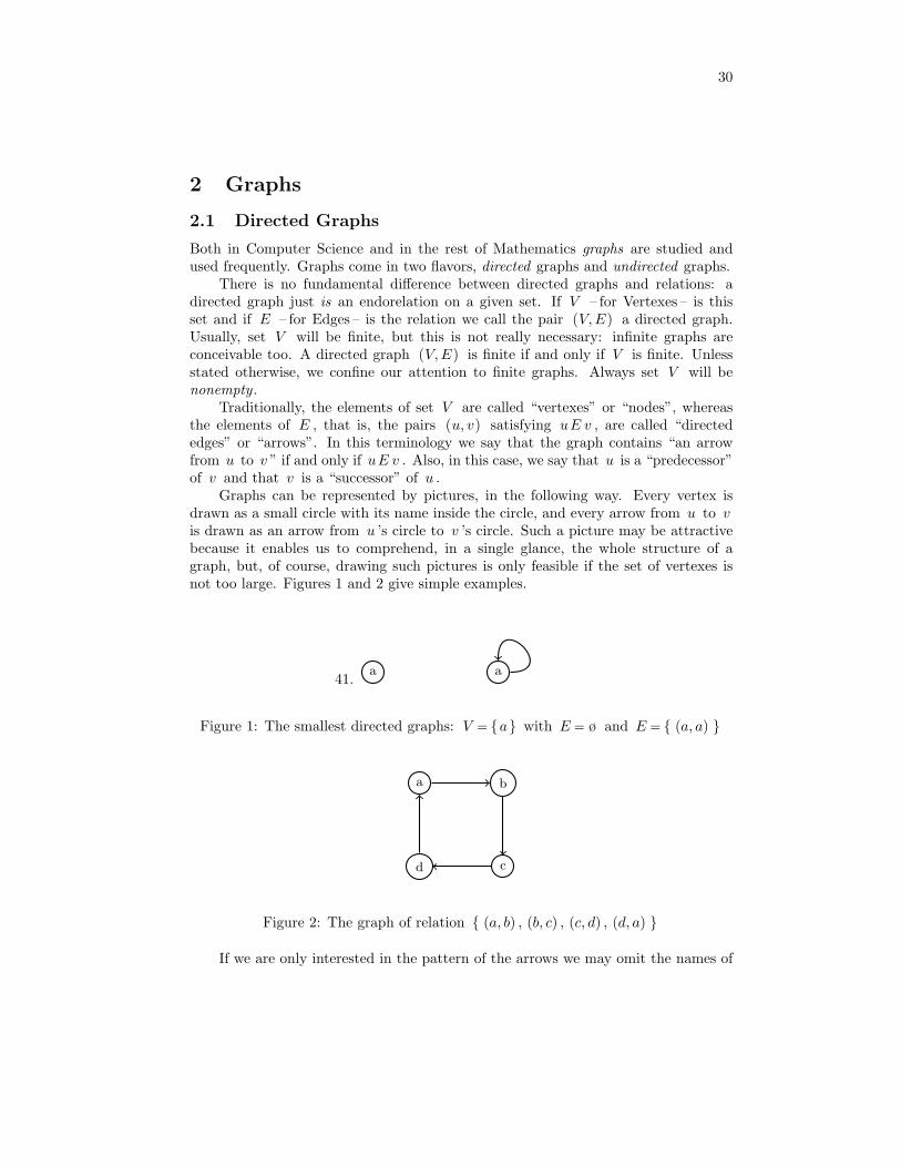
Graphs can be represented by pictures, in the following way. Every vertex isdrawn as a small circle with its name inside the circle, and every arrow from u to vis drawn as an arrow from u ’s circle to v ’s circle. Such a picture may be attractivebecause it enables us to comprehend, in a single glance, the whole structure of agraph, but, of course, drawing such pictures is only feasible if the set of vertexes isnot too large. Figures 1 and 2 give simple examples.

41.a a

Figure 1: The smallest directed graphs: V = a with E = ø and E = (a, a)

a b

cd

Figure 2: The graph of relation (a, b) , (b, c) , (c, d) , (d, a)

If we are only interested in the pattern of the arrows we may omit the names of

31

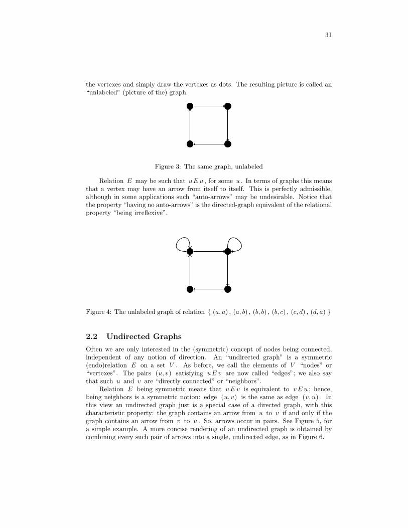
the vertexes and simply draw the vertexes as dots. The resulting picture is called an“unlabeled” (picture of the) graph.

Figure 3: The same graph, unlabeled

Relation E may be such that uE u , for some u . In terms of graphs this meansthat a vertex may have an arrow from itself to itself. This is perfectly admissible,although in some applications such “auto-arrows” may be undesirable. Notice thatthe property “having no auto-arrows” is the directed-graph equivalent of the relationalproperty “being irreflexive”.

Figure 4: The unlabeled graph of relation (a, a) , (a, b) , (b, b) , (b, c) , (c, d) , (d, a)

2.2 Undirected Graphs

Often we are only interested in the (symmetric) concept of nodes being connected,independent of any notion of direction. An “undirected graph” is a symmetric(endo)relation E on a set V . As before, we call the elements of V “nodes” or“vertexes”. The pairs (u, v) satisfying uE v are now called “edges”; we also saythat such u and v are “directly connected” or “neighbors”.

Relation E being symmetric means that uE v is equivalent to vE u ; hence,being neighbors is a symmetric notion: edge (u, v) is the same as edge (v, u) . Inthis view an undirected graph just is a special case of a directed graph, with thischaracteristic property: the graph contains an arrow from u to v if and only if thegraph contains an arrow from v to u . So, arrows occur in pairs. See Figure 5, fora simple example. A more concise rendering of an undirected graph is obtained bycombining every such pair of arrows into a single, undirected edge, as in Figure 6.

32

a b

cd

Figure 5: The graph of (a, b) , (b, a) , (b, c) , (c, b) , (c, d) , (d, c) , (d, a) , (a, d)

Figure 6: The same graph, with undirected edges and unlabeled

There is no fundamental reason why undirected graphs might not also containedges connecting a node to itself. Such edges are called “auto loops”. That is, if uEuthen u is directly connected to itself, so u is a neighbor to itself.1 It so happens,however, that in undirected graphs auto-loops are more a nuisance than useful: manyproperties and theorems obtain a more pleasant form in the absence of auto-loops.

Therefore, we adopt the convention that undirected graphs contain no auto-loops. Formally, this means that an undirected graph is an irreflexive and symmetricrelation.

In the case of finite graphs we sometimes wish to count the number of arrows oredges. We adopt the convention that, in an undirected graph, every pair of directlyconnected nodes counts as a single edge, even though this single edge corresponds totwo arrows in the graph. This reflects the fact that, in a symmetric relation, the pairs(u, v) and (v, u) are indistinguishable. For example, according to this convention,the undirected graph in Figure 6 has four edges.

* * *

We have defined an undirected graph as an irreflexive and symmetric directed graph.Every directed graph can be transformed into an undirected one, just by “ignoring thedirections of the arrows”. In terms of relations this amounts to taking the symmetricclosure of the relation and removal of the auto-arrows: in the undirected graph nodesu and v are neighbors if and only if, in the directed graph, there is an arrow from

1This shows that we should not let ourselves be confused by the connotations of the everyday-lifeword “neighbor”: here the word is used in a strictly technical meaning.

33

u to v or from v to u (or both), provided u 6= v . For example, the directed graphin Figure 4 can thus be transformed into the undirected graph in Figure 6.

2.3 A more compact notation for undirected graphs

We have defined an undirected graph as an irreflexive – no edge between a nodeand itself – and symmetric relation. Although this is correct mathematically, it isnot very practical. For example, the set of edges of the graph in Figure 5 now is (a, b) , (b, a) , (b, c) , (c, b) , (c, d) , (d, c) , (d, a) , (a, d) , in which every edge occurstwice: that nodes a and b , for instance, are connected is represented by the presenceof both (a, b) and (b, a) in the set of edges. Yet, we do wish to consider this connectionas a single undirected edge. It is awkward, then, to have to write down both (a, b)and (b, a) to represent this single edge. We would rather not be forced to distinguishthese pairs.

We obtain a more convenient representation by using two-element2 sets u, v :as set u, v equals set v, u we only need to write this down once. So, in thesequel, an undirected graph will be a pair (V,E) , where V is the set of nodes, asusual, and where E is a set of pairs u, v , with u, v ∈V and u 6= v . For example,the set of edges of the graph in Figure 5 can now be written as: a, b , b, c , c, d , d, a .

In the number of edges, written as #E, we do not double count the edges in twodirections, so in this example we have #E = 4.

Although it is usual to write (., .) for ordered pairs, in which (a, b) 6= (b, a), andin sets elements have no order by which a, b = b, a, in the literature one oftensees (a, b) to denote an edge in an undirected graph.

2.4 Additional notions and some properties

Occasionally, we use infix operators for the relations in directed and undirected graphs.That is, sometimes we write uE v as u→v and we speak of directed graph (V,→ )instead of (V,E) . Similarly, for symmetric relations we sometimes use u∼v insteadof uE v and we speak of undirected graph (V, ∼ ) . So, in this nomenclature, u→vmeans “the graph has an arrow from u to v ” and u∼v means “in the graph u andv are neighbors”.

In a directed graph (V,→ ) , for every node u the number of nodes v satisfyingu→v is called the “out-degree” of u , whereas the number of nodes u satisfyingu→v is called the “in-degree” of v , provided these numbers are finite. Notice thatif V is finite the in-degree and out-degree of every node are finite too. An auto-arrowadds 1 , both to the in-degree and the out-degree of its node.

If relation → is symmetric, so u→v ⇔ v→u for all u, v , then the in-degreeof every node equals its out-degree.

In an undirected graph (V, ∼ ) , the “degree” of a node u is its number ofneighbors, that is, the number of nodes v with u∼v . Thus, the degree of a node

2Undirected graphs contain no auto-edges, so the pair (u, u) is not an edge.

34

in an undirected graph equals the in-degree and the out-degree of that node in theunderlying directed graph.

We write in , out , and deg for “in-degree”, “out-degree”, and “degree” respec-tively.

So for a directed graph (V,E) we have for u, v∈V :

in(v) = #u ∈ V | (u, v) ∈ E out(u) = #v ∈ V | (u, v) ∈ E .

By straightforward addition we obtain:∑v∈V in(v) = #E=

∑u∈V out(u).

For an undirected graph (V,E) we have

deg(u) = #v | u, v ∈ E .

2.1 Theorem. In an undirected graph (V,E) we have

∑v∈V

deg(v) = 2 ∗#E.

Proof. The number of ends of edges can be counted in two ways.In the first one one observes that every edge has two ends, and since there are

#E edges, this number is 2 ∗ #E.In the second one one observes that the degree of a node is the number of ends of

edges to which it is attached. Adding all these yields∑

v∈V deg(v), so these numbersare equal.

* * *

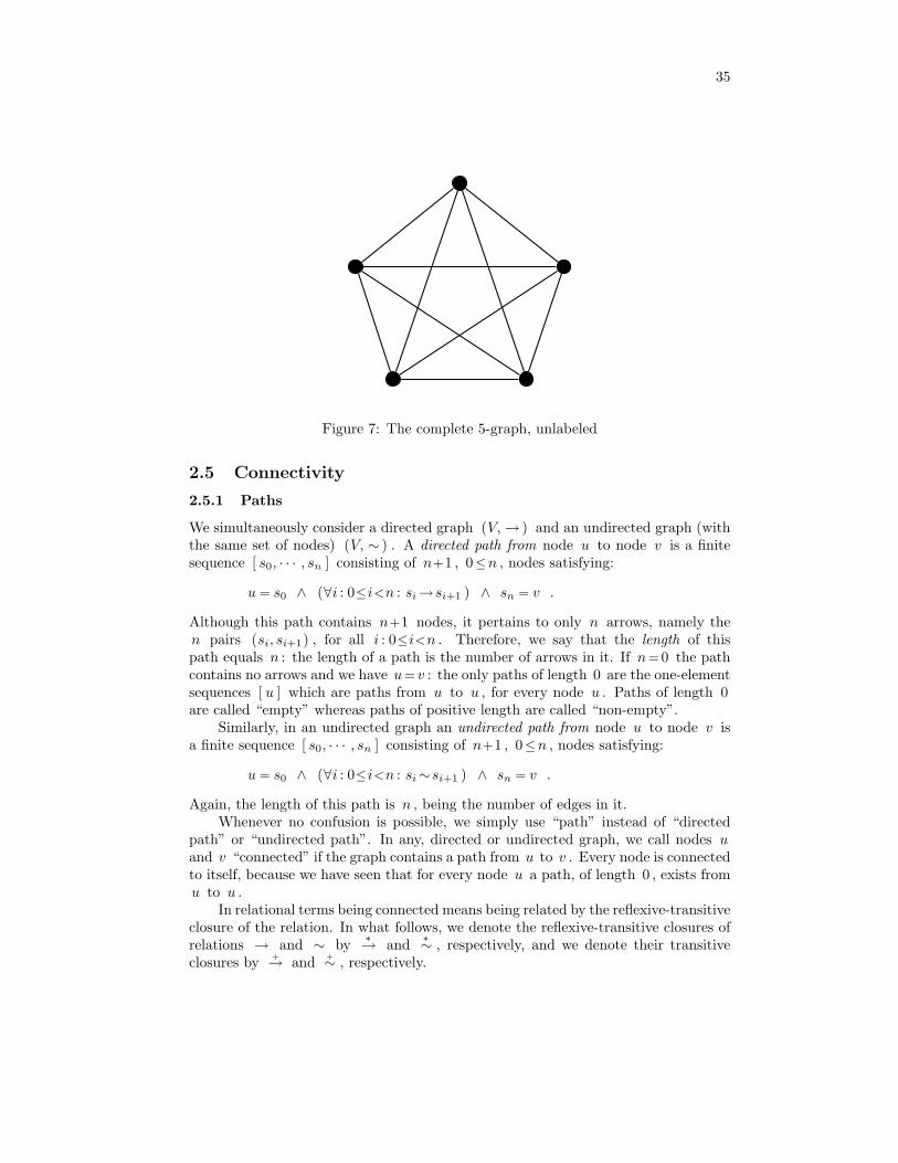
With N for the size of V , so N equals the number of vertexes in the graph, wehave that the degree of every node is at most N−1 . If the degree of a node equalsN−1 then this node is a neighbor of all other nodes. If every node in an undi-rected graph has this property, the graph is called “complete”. Similarly, a directedgraph is complete if it contains an arrow from every node to every node. Thus, thecomplete directed graph corresponds to the complete relation > , whereas the com-plete undirected graph corresponds to the relation >\I (because of the omission ofauto-loops). The complete undirected graph with N nodes is called the completeN -graph. Figure 7, for example, gives a picture of the complete 5 -graph.

35

Figure 7: The complete 5-graph, unlabeled

2.5 Connectivity

2.5.1 Paths

We simultaneously consider a directed graph (V,→ ) and an undirected graph (withthe same set of nodes) (V, ∼ ) . A directed path from node u to node v is a finitesequence [ s0, · · · , sn ] consisting of n+1 , 0≤n , nodes satisfying:

u = s0 ∧ (∀i : 0≤i<n : si→si+1 ) ∧ sn = v .

Although this path contains n+1 nodes, it pertains to only n arrows, namely then pairs (si, si+1) , for all i : 0≤i<n . Therefore, we say that the length of thispath equals n : the length of a path is the number of arrows in it. If n= 0 the pathcontains no arrows and we have u= v : the only paths of length 0 are the one-elementsequences [ u ] which are paths from u to u , for every node u . Paths of length 0are called “empty” whereas paths of positive length are called “non-empty”.

Similarly, in an undirected graph an undirected path from node u to node v isa finite sequence [ s0, · · · , sn ] consisting of n+1 , 0≤n , nodes satisfying:

u = s0 ∧ (∀i : 0≤i<n : si∼si+1 ) ∧ sn = v .

Again, the length of this path is n , being the number of edges in it.Whenever no confusion is possible, we simply use “path” instead of “directed

path” or “undirected path”. In any, directed or undirected graph, we call nodes uand v “connected” if the graph contains a path from u to v . Every node is connectedto itself, because we have seen that for every node u a path, of length 0 , exists fromu to u .

In relational terms being connected means being related by the reflexive-transitiveclosure of the relation. In what follows, we denote the reflexive-transitive closures ofrelations → and ∼ by ∗→ and ∗∼ , respectively, and we denote their transitiveclosures by +→ and +∼ , respectively.

36

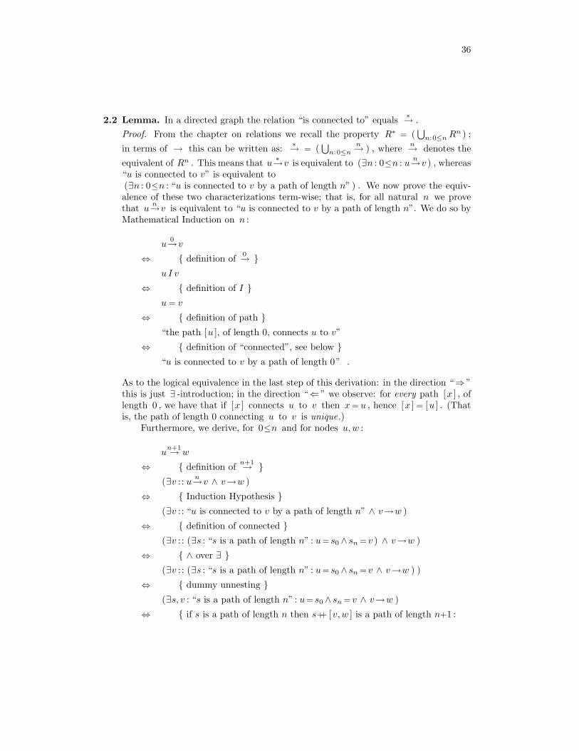
2.2 Lemma. In a directed graph the relation “is connected to” equals ∗→ .Proof. From the chapter on relations we recall the property R∗ = (

⋃n:0≤nR

n ) ;in terms of → this can be written as: ∗→ = (

⋃n:0≤n

n→ ) , where n→ denotes theequivalent of Rn . This means that u ∗→v is equivalent to (∃n : 0≤n : u n→v ) , whereas“u is connected to v” is equivalent to(∃n : 0≤n : “u is connected to v by a path of length n” ) . We now prove the equiv-alence of these two characterizations term-wise; that is, for all natural n we provethat u n→v is equivalent to “u is connected to v by a path of length n”. We do so byMathematical Induction on n :

u0→v

⇔ definition of 0→ u I v

⇔ definition of I u = v

⇔ definition of path “the path [u ], of length 0, connects u to v”

⇔ definition of “connected”, see below “u is connected to v by a path of length 0” .

As to the logical equivalence in the last step of this derivation: in the direction “⇒ ”this is just ∃ -introduction; in the direction “⇐ ” we observe: for every path [x ] , oflength 0 , we have that if [x ] connects u to v then x= u , hence [x ] = [u ] . (Thatis, the path of length 0 connecting u to v is unique.)

Furthermore, we derive, for 0≤n and for nodes u,w :

un+1→ w

⇔ definition of n+1→ (∃v :: u n→v ∧ v→w )

⇔ Induction Hypothesis (∃v :: “u is connected to v by a path of length n” ∧ v→w )

⇔ definition of connected (∃v :: (∃s : “s is a path of length n” : u= s0 ∧ sn = v ) ∧ v→w )

⇔ ∧ over ∃ (∃v :: (∃s : “s is a path of length n” : u= s0 ∧ sn = v ∧ v→w ) )

⇔ dummy unnesting (∃s, v : “s is a path of length n” : u= s0 ∧ sn = v ∧ v→w )

⇔ if s is a path of length n then s++ [v, w ] is a path of length n+1 :

37

dummy transformation (∃t : “t is a path of length n+1” : u= t0 ∧ tn+1 =w )

⇔ definition of connected “u is connected to w by a path of length n+1 ” .

In a very similar way we can prove that the relation “is connected by a non-emptypath length” is equivalent to +→ . Moreover, the proof of the above lemma does notdepend on particular properties of the directed relation → : the lemma and its proofalso are valid for undirected graphs, provided, of course, we replace ∗→ and +→ by∗∼ and +∼ respectively.

* * *

Note that being connected in an undirected graph is a symmetric relation: u isconnected to v if and only if v is connected to u , because [ s0, · · · , sn ] is a pathfrom u to v if and only if the reverse of s , that is, the sequence [ sn, · · · , s0 ] , is apath from v to u .

In directed graphs, being connected is not necessarily symmetric, of course: theexistence of a directed path (usually) does not imply the existence of directed path inthe reverse direction.

2.5.2 Path concatenation

Let s be a directed path of length m from node u to node v , and let t be a directedpath of length n from node v to node w . So, the end point of s , which is v , equalsthe starting point of t , that is, we have sm = t0 .

From s and t we can now construct a directed path, of length m+n , fromnode u to node w ; this is called the “concatenation” of s and t , and we denote itby s++ t . For s and t paths of length m and n , respectively, their concatenations++ t is a path of length m+n , defined as follows:

(s++ t)i = si , for 0≤ i≤m(s++ t)m+i = ti , for 0≤ i≤n

Keep in mind that s++ t is defined only if sm = t0 , and this is implied by thisdefinition: on the one hand (s++ t)m = sm , on the other hand (s++ t)m = t0 . Inthis case, s++ t is a path from u to w indeed. This we prove as follows:

(s++ t)0

= definition of ++ s0

= s is a path from u to v

38

u ,

as required; and, for 0≤ i<m :

(s++ t)i→ (s++ t)i+1

= definition of ++ si→ si+1

= s is a path of length m true

as required; and, for 0≤ i<n :

(s++ t)m+i→ (s++ t)m+i+1

= definition of ++ ti→ ti+1

= t is a path of length n true

as required; and, finally:

(s++ t)m+n

= definition of ++ tn

= t is a path from v to w w ,

as required.

Concatenation of undirected paths is defined in exactly the same way: here con-catenation is actually an operation on sequences of nodes, and the difference between→ and ∼ , that is, the difference between directed and undirected, only plays a rolein the interpretation of such sequences as paths.

We now conclude that, both in directed and in undirected graphs, if a path s ,say, exists from node u to node v and if a path t , say, exists from node v to nodew , then also a path exists from node u to node w , namely s++ t . Thus we haveproved the following lemma.

2.3 Lemma. Both in directed and in undirected graphs, the relation “is connected to”is transitive.2

2.5.3 The triangular inequality

Every path in a graph has a length, which is a natural number. Every non-emptyset of natural numbers has a smallest element. Therefore, if node u is connected tonode v we can speak of the minimum of the lengths of all paths from u to v . Thiswe call the “distance” from u to v . Because, in undirected graphs, connectedness is

39

symmetric, we have, in undirected graphs, that the distance from u to v is equal tothe distance from v to u .

If u is not connected to v we define, for the sake of convenience, the distancefrom u to v to be ∞ (“infinity”), because ∞ can be considered, more or less, as theidentity element of the minimum-operator. Note, however, that ∞ is not a naturalnumber and that we must be very careful when attributing algebraic properties toit. For example, it is viable to define ∞+n = ∞ , for every natural n , and even∞+∞ = ∞ , but ∞−∞ cannot be defined in a meaningful way. An importantproperty is:

(0) n <∞ , for all n ∈ Nat ;

(1) n ≤∞ , for all n ∈ Nat∪∞ .

We denote the distance from u to v by dist(u, v) . Then, function dist is definedas follows, for all nodes u, v :

dist(u, v) = ∞ , if u is not connected to v ;

dist(u, v) = (minn : 0≤n ∧ “a path of length n exists from u to v” : n ) ,if u is connected to v .

Function dist now satisfies what is known in Mathematics as the “triangular inequal-ity”. This lemma holds for both directed and undirected graphs.

2.4 Lemma. All nodes u, v, w satisfy: dist(u,w) ≤ dist(u, v) + dist(v, w) .

Proof. By (unavoidable) case analysis. If dist(u, v) =∞ or dist(v, w) =∞ then alsodist(u, v) + dist(v, w) = ∞ ; now, by property (1) , we have dist(u,w) ≤∞ , so weconclude, for this case: dist(u,w) ≤ dist(u, v) + dist(v, w) , as required.

Remains the case dist(u, v) <∞ and dist(v, w) <∞ . In this case, paths existfrom u to v and from v to w . Let s be a path, of length m , from u to v andlet t be a path, of length n , from v to w . Then, as we have seen in the previoussubsection, s++ t is a path, of length m+n , from u to w . By the definition of dist ,we conclude: dist(u,w) ≤ m+n . As this inequality is true for all such paths s andt , it is true for paths of minimal length as well. Hence, also for this case we have:dist(u,w) ≤ dist(u, v) + dist(v, w) , as required.

2.5.4 Connected components

A directed graph (V,→ ) is strongly connected if every node is connected to everynode, that is, if there is a directed path from every node u to every node v . Inrelational terms, this means that ∗→ = > . The adverb “strongly” stresses the factthat, in directed graphs, strong connectedness is a symmetric notion: for every twonodes u, v there is a path from u to v and there is path from v to u .

40

An undirected graph is connected if every pair of nodes is connected by a path.Relationally, a graph is connected if and only if ∗∼ = > . As we have seen, in undi-rected graphs connectedness is symmetric. It even is an equivalence relation. Aconnected component is a maximal subset of the nodes of the graph that is connected:the connected components of an undirected graph are the equivalence classes of ∗∼ .

Figure 8: An undirected graph with 3 connected components

2.6 Cycles

A cycle in a graph is a non-trivial path from a node to itself. For undirected graphs aproper definition of ‘non-trivial’ needs some care. Generally, a graph may contain fewcycles, many cycles, or no cycles at all. In the latter case the graph is called acyclic.

2.6.1 Directed cycles

In a directed graph a cycle is a (directed) path from a node to itself. For example, ifa→b and b→a then the path [ a , b , a ] is a cycle, and so is the path [ b , a , b ] .Although these are different paths they constitute, in a way, the same cycle. Thesimplest possible case of a directed cycle is [ a , a ] , namely if a→a .

a b

Figure 9: A simple directed cycle

a

Figure 10: An even simpler cycle

41

2.6.2 Undirected cycles

In undirected graphs the notion of cycles is somewhat more complicated. For example,if, in undirected graph (V, ∼ ) , we have a∼b and, hence, also b∼a , then [ a , b , a ]is a path from node a to itself. Yet, we do not wish to consider this a cycle. Moregenerally, we do not wish the pattern [ · · · , a , b , a , · · · ] to occur anywhere in acycle: in a cycle, every next edge should be different from its predecessor. As aconsequence, in an undirected graph the smallest possible cycle involves at least threenodes and three edges. Some texts require even stronger conditions for a path to bea cycle, for instance, that no node occurs more than once. We choose for the weakestversion only excluding directly going back.

These considerations give rise to the following definition.

2.5 Definition. An undirected cycle is a path [ s0, · · · , sn ] , of length n ≥ 3, for whichs0 = sn and (∀i : 0≤i≤n−2 : si 6= si+2 ) and sn−1 6= s1.

The first of these conditions expresses that the path’s last node equals its first node– thus “closing the cycle” – , and the rest expresses that every two successive edgesin the cycle are different. The conjunct sn−1 6= s1 really is needed here: the “last”edge, sn−1, sn , which is the same as sn−1, s0 , and the “first” edge, s0, s1 ,are successive too, which must be different as well.

In Figure 14, for example, we have that [ a, b, d, b, c, a ] is not a cycle, because itcontains edge b, d twice in succession. Without the conjunct sn−1 6= s1 , however,the path [ d, b, c, a, b, d ] would be a cycle, which is undesirable: whether or not acertain collection of nodes constitutes a cycle should not depend on which node is thefirst node of the path representing that cycle.

a b c

Figure 11: No cycles at all

a b

Figure 12: Not even an (undirected) graph

Thus we obtain the following lemma, which expresses that cycles are “invariantunder rotation”. This lemma is useful because it allows us to let any node in a cyclebe the starting node of the path representing that cycle.

42

Figure 13: The smallest undirected cycle

a b

c

d e

f

Figure 14: [ a, b, d, e, f, d, b, c, a ] is a cycle, [ a, b, d, b, c, a ] is not

2.6 Lemma. [Rotation Lemma] For every natural n , 3≤n , a path [ s0, s1, · · · , sn−1, s0 ]is a cycle if and only if the path [ s1, · · · , sn−1, s0, s1 ] is a cycle.2

In a similar way we have a lemma for reversing a cycle.

2.7 Lemma. [Reversal Lemma] For every natural n , 3≤n , a path [ s0, s1, · · · , sn−1, s0 ]is a cycle if and only if the path [ s0, sn−1, sn−2, · · · , s1, s0 ] is a cycle.2

2.7 Euler and Hamilton cycles

2.7.1 Euler cycles

In a undirected graph a cycle with the property that it contains every edge of thegraph exactly once is called an Euler cycle.

2.8 Theorem. For every connected graph (V, ∼ ) with ∼ non-empty we have

(V, ∼ ) contains an Euler cycle ⇔ (∀v : v∈V : deg(v) is even) .

Proof. By mutual implication.

“⇒ ”: We consider an Euler cycle in graph (V, ∼ ) . Let v be a node. Wherever voccurs in the Euler cycle v has a predecessor u , say, in the cycle and a successorw , say, in the cycle. This means that u, v, w are all different and u∼ v and v ∼w .Thus, all edges associated with v occurring in the Euler cycle occur in pairs; hence,the total number of edges associated with v occurring in the Euler cycle is even.

43

Because the cycle is an Euler cycle all of v ’s edges occur in the Euler cycle; hence,deg(v) is even.

“⇐ ”: Assuming (∀v : v∈V : “deg(v) is even”) we prove the existence of an Eulercycle by sketching an algorithm for the construction of an Euler cycle. This algorithmconsists of two phases. In the first phase a collection of (one or more) cycles is formedsuch that every edge of the graph occurs exactly once in exactly one of these cycles.In the second phase, the cycles in this collection are combined into larger cycles, thusreducing the number of cycles in the collection while retaining the property that everyedge of the graph occurs exactly once in exactly one of the cycles in the collection.As soon as this collection contains only one cycle, this one cycle is a Euler cycle.

first phase: Initially all edges are white. The property (∀v : v∈V : “deg(v) is even”)will remain valid for the subgraph formed by V and the white edges only: it is aninvariant of this phase. Another invariant is that all red edges form a collection ofcycles with the property that every red edge of the graph occurs exactly once in exactlyone of these cycles. Initially this is true because there are no red edges: initially thecollection of red cycles is empty. If, on the other hand, all edges are red the collectionof red cycles comprises all edges of the graph, and the first phase terminates. As longas the graph contains at least one white edge, the following step is executed.

Select a white edge, s0, s1 , say. Because deg(s1) is even, node s1 has aneighbor s2 , say, that differs from s0 and such that edge s1, s2 is white as well.Repeating this indefinitely yields an infinite sequence si :0≤i of nodes, pairwise con-nected by white edges. As the graph is finite, this sequence contains a sub-path[ sp, · · · , sq ] , for some p, q with 0≤ p< q , that is a cycle, comprising white edgesonly. Now all white edges in this cycle are turned red. Because, for every node in thiscycle, its associated edges occur in pairs, the number of white edges associated withany node in this cycle is even and, as a result, the degree of all nodes remains evenunder reddening of the white edges in this cycle. This process is repeated as longas white edges exist. Because in a undirected graph every cycle contains at least 3edges the number of white edges thus decreases (by at least 3 ), this first phase willnot go on forever, and will end in a situation where no white edges exist any more.

second phase: The second phase terminates if the collection of red cycles contains onlyone cycle. As long as this collection contains at least two cycles it takes two cyclesthat have a node in common. This is always possible due to the assumption that thegraph is connected: if for a cycle all nodes are on none of the other cycles, this cycleis isolated and does not admit a path to any node on the other cycles, contradictingconnectedness. Now these two cycles with a node v in common can be joined to asingle cycle: if the one cycle is a path s from v to v and the other cycle is a path tfrom v to v, then the concatenation of s and t is a cycle covering both original cycles.It satisfies the cycle condition since s and t are disjoint. In this way the total numberof cycles decreases, while still every edge of the original graph occurs exactly once asan edge of one of the cycles. This process is repeated until only one cycle remainsand all cycles have been glued together; by construction this cycle is an Euler cycle.

44

This proof of existence of an Euler cycle is constructive, and of a quite algorithmicnature. In fact, it gives rise to an algorithm to construct an Euler cycle in anyconnected graph in which all degrees are even, that is linear in the number of edges.

2.7.2 Hamilton cycles

In a (directed or undirected) graph a cycle with the property that it contains everynode of the graph exactly once is called a Hamilton cycle.

A naive algorithm to compute whether a given graph contains a Hamilton cycleis conceptually simple: enumerate all cycles and check whether any of them is aHamilton cycle. This naive algorithm is quite inefficient, of course, but really efficientalgorithms are not (yet) known: the problem to decide whether a graph contains aHamilton cycle is NP-hard , which in practice means that all algorithms will requirean amount of computation time that grows exponentially with the size of the graph.

Notice the contrast in complexity between the notion of Euler and Hamiltoncycles. On the one hand, Theorem 2.8 provides a simple algorithm to evaluate theexistence of an Euler cycle – just calculate the degrees of the nodes – , and its proofcontains a relatively straightforward algorithm for the construction of an Euler cy-cle. On the other hand, calculating the existence of an Hamilton cycle, let aloneconstruction of one, is NP-hard.

Thus, two seemingly similar notions – Euler cycles and Hamilton cycles – happento have essentially different properties.

2.7.3 A theorem on Hamilton cycles

We consider finite, undirected graphs, with at least 4 nodes. We present a theoremgiving a sufficient condition for the existence of Hamilton cycles, namely if the graphcontains “sufficiently many” edges. In our case the notion of “sufficiently many” andthe theorem take the following shape.

2.9 Theorem. We consider an undirected graph with n nodes, 4≤n . If, for every twounconnected nodes, the sum of their degrees is at least n , then the graph contains aHamilton cycle.2

To formalize this, let V be a (fixed) set of nodes, with n = #V , 4≤n . In whatfollows variables u, v, p, q range over V , with p 6= q . The set E of edges is variable;that is, as a function of E we define predicates P and H , as follows:

P (E) = (∀u, v : u 6= v : u, v 6∈E ⇒ deg(u) + deg(v) ≥ n ) , and:

H(E) = “graph (V,E) contains a Hamilton cycle ” .

Predicate P formalizes our particular version of “sufficiently many”: P expressesthat, for every two unconnected nodes, the sum of their degrees is at least n .

Both P and H are monotonic, as follows:

45

monotonicity: For all E and for any two nodes p, q :P (E) ⇒ P (E ∪ p, q ) , and:

H(E) ⇒ H (E ∪ p, q ) .2

In addition, for the extreme cases, the empty graph ⊥ and the complete graph > ,we have:

¬ (P (⊥)) ∧ ¬ (H(⊥)) ∧ P (>) ∧ H(>) .

The theorem now states that every graph satisfying predicate P contains at least oneHamilton cycle.

2.10 Theorem. (∀E :: P (E) ⇒ H(E) ) .2

We present two proofs for this theorem. These proofs are essentially the same, butthey differ in their formulation. The crucial part in both proofs is the following:

Core Property: For set E of edges and for any two nodes p, q with ¬ (p, q ∈E) :

P (E) ∧ H (E ∪ p, q ) ⇒ H(E) .2

Notice that the Core Property also holds if p, q ∈E , but in a trivial way only: thenH (E ∪ p, q ) = H(E) , so in this case the property is void.

We will present a proof for the Core Property later, but first we will show howit is used in the proofs of the Theorem.

2.7.4 A proof by contradiction

The first proof runs as follows, by contradiction. That is, we suppose that the Theoremis false. Then, there exists a set F of edges such that P (F ) and ¬ (H(F )) . Because¬ (H(F )) and H(>) , and because F ⊆> , there also exists a “turning point”, thatis, a set E of edges and a pair p, q of nodes such that:

F ⊆E ∧ ¬ (H(E)) ∧ H (E ∪ p, q ) .

Notice that, because of ¬ (H(E)) ∧ H (E ∪ p, q ) , we have – Leibniz! – thatE 6= E ∪ p, q , hence p, q 6∈E .

Because of the monotonicity of P , and because P (F ) and F ⊆E , set E satisfiesP (E) too. Now, from P (E) and H (E ∪ p, q ) we conclude, using the CoreProperty, H(E) . In conjunction with the assumed ¬ (H(E)) we obtain the desiredcontradiction.

46

2.7.5 A more explicit proof

The reasoning in the previous proof is somewhat strange: the assumption ¬ (H(E))is not really used in the proof proper: it is only used to conclude a contradiction.Therefore, we should be able to construct a more direct proof. In addition what does“there exists a ‘turning point’ ” really mean, mathematically speaking?

Because of the monotonicity of P we have P (E) ⇒ P (E ∪ p, q ) ; therefore,by means of elementary propositional calculus, the Core Property can be rewrittenthus:

(2) (P (E ∪ p, q ) ⇒ H (E ∪ p, q ) ) ⇒ (P (E) ⇒ H(E) ) ,

and this smells very strongly of a proof by Mathematical Induction. As a matter offact, this is Mathematical Induction, albeit in a somewhat unusual direction, namelyfrom larger towards smaller.

Firstly, we have H(>) – the complete graph contains a Hamilton cycle, verymany even – , so we also have P (>) ⇒ H(>) . This is the basis of the induction.

Secondly, property (2) now represents the induction step. Because every set Eof edges can be obtained from a larger set E ∪ p, q , with p, q 6∈E , we aredone.

Notice that the fact that the collection of all possibles sets of edges is finite3 is ofno consequence: although usually applied to infinite sets the principle of MathematicalInduction is perfectly valid in a finite setting.

2.7.6 Proof of the Core Property

We repeat the Core Property, which is the essential part of both proofs of the Theorem.

Core Property: For set E of edges and for any two nodes p, q with p, q 6∈E :

P (E) ∧ H (E ∪ p, q ) ⇒ H(E) .2

To prove this we assume that E is a set of edges and p, q are different nodes, suchthat p, q 6∈E , satisfying P (E) and H (E ∪ p, q ) . The latter means that thegraph (V , E ∪ p, q ) contains a Hamilton cycle. If such a Hamilton cycle doesnot contain edge p, q , then it also is a Hamilton cycle in the graph (V,E) ; hence,H(E) and in this case we are done.

So, remains the case that (V , E ∪ p, q ) contains a Hamilton cycle thatdoes contain edge p, q . Now we have to prove H(E) , that is, we must prove that(V,E) contains a Hamilton cycle as well, that is, without edge p, q .

For this purpose, let [ s0, s1, · · · , sn ] be a Hamilton cycle in (V , E ∪ p, q ) .This means that si | 0≤i<n = V – recall that n = #V – , that sn = s0 , and that(∀i : 0≤i<n : si, si+1 ∈E ∪p, q ) . We assume that this cycle contains edgep, q and, without loss of generality, we assume that s0 = p and s1 = q .

3for our fixed , finite set of nodes

47

s0 = p s1 = q

s2

shsh+1

sn−1

Figure 15: a Hamilton cycle, with edge p, q

In this setting we prove that (V,E) contains a Hamilton cycle. To construct aHamilton cycle not containing edge p, q we take the Hamilton cycle introducedabove, containing edge p, q , as a starting point. Removal of edge p, q destroysthe cycle, and what remains is a path connecting s1 , that is q , to s0 , that is p , thatstill contains all nodes of the graph and all edges of which are in E .Now we must restore the cycle by somehow reconnecting p and q , using edges inE only. We do so by selecting an index h in the interval [ 2 . . n−1 ) such that bothp, sh ∈E and q, sh+1 ∈E . To show that this is possible we need the theorem’sassumption P (E) , which was defined as:

(∀u, v : u 6= v : u, v 6∈E ⇒ deg(u) + deg(v) ≥ n ) .

Applying this to p, q and using p, q 6∈E we obtain:

(3) deg(p) + deg(q) ≥ n .

Let x = # i∈ [ 2 . . n−1 ) | p, si ∈E and let y = #j ∈ [ 2 . . n−1 ) | q, sj+1 ∈E ;now we calculate:

deg(p) + deg(q) ≥ n

⇔ definition of deg (twice), using s0 = p and s1 = q # i∈ [ 1 . . n ) | s0, si ∈E + #j ∈ [ 2 , n ] | s1, sj ∈E ≥ n

⇔ split off i= 1 and i=n−1 , using s0, s1 6∈E and sn−1, sn ∈E 1 + # i∈ [ 2 . . n−1 ) | s0, si ∈E + #j ∈ [ 2 , n ] | s1, sj ∈E ≥ n

⇔ split off j = 2 and j =n , using s1, s2 ∈E and s1, sn 6∈E

48

s0 = p s1 = q

s2

shsh+1

sn−1

Figure 16: The remains of the cycle, after removal of edge p, q

1 + # i∈ [ 2 . . n−1 ) | s0, si ∈E + 1 + #j ∈ [ 3 . . n ) | s1, sj ∈E ≥ n

⇔ dummy transformation j := j+1 1 + # i∈ [ 2 . . n−1 ) | s0, si ∈E + 1 + #j ∈ [ 2 . . n−1 ) | s1, sj+1 ∈E ≥ n

⇔ definitions of x and y , using s0 = p and s1 = q 1 + x + 1 + y ≥ n

⇔ calculus x + y ≥ n− 2 .

So, the number of indexes i in the interval [ 2 . . n−1 ) for which p, si ∈E plusthe number of indexes i in the range [ 2 . . n−1 ) for which q, si+1 ∈E is at leastn− 2 . The size of the interval [ 2 . . n−1 ) , however, only is n− 3 ; hence the two setsof indexes have a non-empty intersection: there exists an index h , h∈ [ 2 . . n−1 ) ,such that both p, sh ∈E and q, sh+1 ∈E .

For every such an index h , [ s0, sh, · · · , s2, s1, sh+1, · · · , sn−1, sn ] is a Hamiltoncycle in the graph (V,E) . Because we have shown the existence of such an h , weconclude the existence of a Hamilton cycle in (V,E) , which was our goal.

remark: The existence of an index h in the interval [ 2 . . n−1 ) implies thatthis interval is nonempty, that is, 2 <n−1 , which boils down to 4≤n .Hence, the proofs of the Theorem presented here are only valid for graphswith at least 4 nodes. It can be easily verified that the Theorem also holdsfor n= 3 : the complete 3 -graph – a “triangle” – is the only one satisfyingpredicate P , and a “triangle” is a Hamilton cycle. For n< 3 the Theorem

49

does not hold.2

s0 = p s1 = q

s2

shsh+1

sn−1

Figure 17: a Hamilton cycle, without edge p, q

2.8 Ramsey’s theorem

2.8.1 Introduction

We are having a party at which every two guests either do know each other or donot know each other. If the number of guests at the party is “large enough” then theparty has at least 5 guests all of which either do know one another or do not knowone another. How large must the party be for this to be true?

F.P. Ramsey has developed some theory for the treatment of problems like this.This theory makes it possible to draw rather global conclusions about undirectedgraphs, independently of their actual structure.

To illustrate this we present a simple theorem that represents his work. In theabove example the guests at the party can be considered the nodes of an undirectedgraph. Any two nodes are connected by an edge if and only if the two correspondingguests do know each other. A set of 5 guests all of which do know one another thenamounts to a subgraph of size 5 that is complete, that is, we say that the whole graphcontains a complete 5-graph. How do we formulate, on the other hand, that from aset of 5 guests every two guests do not know each other? Well, this means that thewhole graph contains 5 nodes every two of which are not connected.

We might as well, however, consider the complement graph, in which two nodesare connected by an edge if and only if the two corresponding guests do not know

50

each other. As a matter of fact, the problem as stated is symmetric in the notionsof “knowing each other” and “not knowing each other”. It is, therefore, awkwardto destroy this symmetry by representing the one concept by the presence of edgesand the other concept by their absence. Moreover, we have two possibilities here, thechoice between which is irrelevant.

To restore the symmetry we, therefore, consider a complete undirected graph, ofwhich the set of edges has been partitioned into two subsets – or more than two, inthe more general case of Ramsey’s theory – . The one subset then represents the pairsof guests who know each other and the other subset represents the pairs of guestswho do not know each other.

Partitioning a set into (disjoint) subsets can be represented conveniently by col-oring . In our case, partitioning the edges of a complete graph into two subsets can berepresented by coloring each edge with one out of two colors. (And, of course, withmore than two colors we can represent partitionings into more than two subsets.)Now, an edge of the one color may represent a pair of guests who do know each other,whereas an edge of the other color may represent a pair of guests who do not knoweach other. Thus, the symmetry between “knowing” and “not knowing” is restored.

2.8.2 Ramsey’s theorem

We consider finite, complete, undirected graphs only. For the sake of brevity, we willuse “k -graph” for the “complete k-graph”, for any natural k , 2≤ k . Formally, acoloring of a graph’s edges is a function from the set of edges to the set of colorsused, red , blue , say, if two colors are sufficient. So, a coloring is a function of typeE→ red , blue , and if c is such a coloring, then for any edge u, v we have eitherc(u, v ) = red or c(u, v ) = blue , but not both simultaneously, as we presumethat red 6= blue : every edge has only one color. In what follows we use variables cand d to denote colorings.

Again for brevity’s sake, we say that the k -graph “contains a red m-graph” ifthe nodes of the k -graph contain a subset of m nodes such that all edges connectingthese nodes are red; that is, these m nodes together with their edges constitute acompletely red m-graph as a subgraph of the k -graph, for any k,m with 2≤m≤ k .

As an example, notice that the 2-graph has two nodes only, connected by onesingle edge; hence, the proposition “the k -graph contains a red 2-graph” is equivalentto the proposition “the k -graph contains at least one red edge”.

The proposition “the k -graph contains a red m-graph” depends on the parame-ters k and m , of course, but also on the actual coloring. So, it is a predicate withthree parameters. Calling this predicate Rd , we define it as follows, together with asimilar predicate Bl , for the color blue, for all k, c,m with 2≤m≤ k :

Rd (k, c,m) ⇔ “the k -graph with coloring c contains a red m-graph” , and:

Bl (k, c,m) ⇔ “the k -graph with coloring c contains a blue m-graph” .

These predicates are monotonic, in the following way. Suppose Rd (k, c,m) , for somek, c,m . Then we also have Rd (k+1 , c ,m) , provided we consider the coloring of the

51

(k+1)-graph as an extension of the coloring of the k -graph – both colorings beingdenoted here by the very same c – , just as the (k+1)-graph can be viewed as anextension of the k -graph. For this purpose we consider the k+1 nodes of the (k+1)-graph as a set of k nodes, forming a k -graph, plus one additional node, which mayremain anonymous. Every coloring of the (k+1)-graph thus induces a coloring of thek -graph; as stated, function c denotes either coloring.

Ramsey’s theorem now is about a function R , say, defined as follows, for allm,n with 2≤m and 2≤m :

R(m,n) = “the smallest of all natural numbers k satisfying:(∀c :: Rd (k, c,m) ∨ Bl (k, c, n) ) ” .

The function value R(m,n) is only well-defined, of course, if at least one naturalnumber k exists satisfying (∀c :: Rd (k, c,m) ∨ Bl (k, c, n) ) : only then we can speakof the smallest such number. Notice that, by definition, if R(m,n) = p then forevery k , p≤ k , the k -graph contains at least one red m-graph or contains at leastone blue n-graph (or both).

The following theorem states that such natural numbers exist and provides anupper bound for R(m,n) .

2.11 Theorem. (Ramsey)

R(m,n) ≤(m+n−2m−1

), for all m,n : 2≤m ∧ 2≤n .

2

Notice that, by definition, R(m,n) is symmetric in m and n , that is, we have:R(m,n) = R(n,m) , because for every coloring c satisfying Rd (k, c,m) ∨ Bl (k, c, n)a coloring d exists – which one? – satisfying Rd (k, d, n) ∨ Bl (k, d,m) . The expres-

sion(m+n−2m−1

)does not look symmetric, at least, not at first sight. Yet, it is,

because binomial coefficients satisfy the following, general property:(m+nm

)=

(m+nn

), for all m,n : 1≤m ∧ 1≤n ,

as a result of which we also have:(m+n−2m−1

)=

(m+n−2n−1

).

Proof of the Theorem: By Mathematical Induction on the value of m+n ;that is, the Induction Hypothesis is:

R(p, q) ≤(p+q−2p−1

), for all p, q : 2≤ p ∧ 2≤ q ∧ p+q<m+n .

52

We distinguish 3 cases.

Firstly, 2≤m ∧ n= 2 : We consider the m-graph. Let c be the color-ing in which all edges of the m-graph are red, so this particular c yieldsRd (m, c,m) . For every other coloring c we have that not all edges of the m-graph are red, so the m-graph contains at least one blue edge, which meansBl (m, c, 2) , for all other c . Combining these cases we obtain (∀c :: Rd (m, c,m) ∨ Bl (m, c, 2) ) ,from which we conclude that R(m,n) ≤m . (Actually, we have R(m,n) = mbecause no smaller graph contains a red m-graph, but the upper bound is all

we need.) Now m =

(m+2−2m−1

), so we conclude R(m,n) ≤

(m+2−2m−1

),

as required.

Secondly, m= 2 ∧ 2≤n : By symmetry with the previous case.

Thirdly, 3≤m ∧ 3≤n : We need an additional property, to be proved later;the need of this property is inspired by a well-known property of binomialcoefficients:

R(m,n)

≤ • property of R , see below, using 3≤m ∧ 3≤n R(m−1 , n) +R(m,n−1)

≤ Induction Hypothesis (twice) (m+n−3m−2

)+

(m+n−3m−1

)= property of binomial coefficients (

m+n−2m−1

).

2

In the above proof of the Theorem we have used the following property of R , whichconstitutes the core of the proof.

property: R(m,n) ≤ R(m−1 , n) +R(m,n−1) , for all m,n : 3≤m ∧ 3≤n .

proof: Let k = R(m−1 , n) +R(m,n−1) . To prove that R(m,n) ≤ k itsuffices to prove Rd (k, c,m) ∨ Bl (k, c, n) , for all colorings c . Therefore,let c be a coloring of the k -graph. Let v be a node of the k -graph and inwhat follows dummy u also ranges over the nodes of the k -graph. We definesubsets X and Y of the nodes, as follows:

X = u∈V | u 6= v ∧ c(u, v ) = red , and:

Y = u∈V | u 6= v ∧ c(u, v ) = blue .

53

Then X and Y and v partition the nodes of the k -graph, so we have:

#X + #Y + 1 = R(m−1 , n) +R(m,n−1) .

From this it can be derived that R(m−1 , n) ≤ #X ∨ R(m,n−1) ≤ #Y ,by contraposition:

#X < R(m−1 , n) ∧ #Y < R(m,n−1)

⇔ all values here are integers #X ≤ R(m−1 , n)−1 ∧ #Y ≤ R(m,n−1)−1

⇒ monotonicity of addition #X+#Y ≤ R(m−1 , n) +R(m,n−1) − 2

⇔ all values here are integers #X+#Y +1 < R(m−1 , n) +R(m,n−1)

⇒ < is irreflexive #X+#Y +1 6= R(m−1 , n) +R(m,n−1) ,

which settles the issue.We now prove the required property, Rd (k, c,m) ∨ Bl (k, c, n) , by dis-

tinguishing the two cases of this disjunction.

Case R(m−1 , n) ≤ #X : From the definition of R we conclude, for our col-oring c , that either Rd (#X, c ,m−1) or Bl (#X, c , n) . If Rd (#X, c ,m−1)then X contains a red (m−1)-graph. By definition of X , we also havec(u, v ) = red , for all u∈X ; hence, X ∪v contains a red m-graph,which implies Rd (k, c,m) as well. If, on the other hand, Bl (#X, c , n) thenwe also have Bl (k, c, n) . In both cases we have Rd (k, c,m) ∨ Bl (k, c, n) ,which concludes this case.

Case R(m,n−1) ≤ #Y : By symmetry.2

2.8.3 A few applications

A party containing 5 guests all knowing one another or all not knowing one anothercan now represented as a complete graph containing a red 5 -graph or a blue 5 -graph.So, asking for the smallest such party is asking for the value of R(5, 5) . As upper

bound for R(5, 5) , Ramsey’s theorem now gives(

84

), which equals 70 . Further

investigation of this problem has revealed that R(5, 5) ∈ [ 43 , 49 ] ; what is the actualvalue of R(5,5) still is an open problem!

* * *

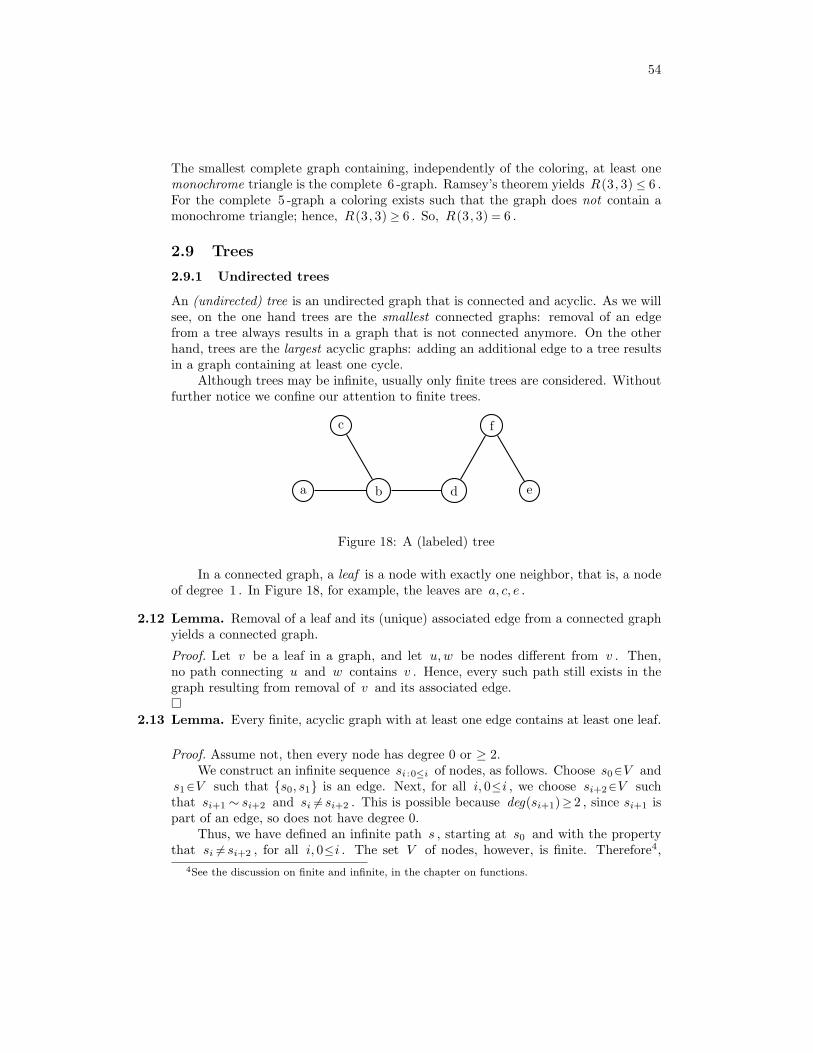
54

The smallest complete graph containing, independently of the coloring, at least onemonochrome triangle is the complete 6 -graph. Ramsey’s theorem yields R(3, 3) ≤ 6 .For the complete 5 -graph a coloring exists such that the graph does not contain amonochrome triangle; hence, R(3, 3) ≥ 6 . So, R(3, 3) = 6 .

2.9 Trees

2.9.1 Undirected trees

An (undirected) tree is an undirected graph that is connected and acyclic. As we willsee, on the one hand trees are the smallest connected graphs: removal of an edgefrom a tree always results in a graph that is not connected anymore. On the otherhand, trees are the largest acyclic graphs: adding an additional edge to a tree resultsin a graph containing at least one cycle.

Although trees may be infinite, usually only finite trees are considered. Withoutfurther notice we confine our attention to finite trees.

a b

c

d e

f

Figure 18: A (labeled) tree

In a connected graph, a leaf is a node with exactly one neighbor, that is, a nodeof degree 1 . In Figure 18, for example, the leaves are a, c, e .

2.12 Lemma. Removal of a leaf and its (unique) associated edge from a connected graphyields a connected graph.

Proof. Let v be a leaf in a graph, and let u,w be nodes different from v . Then,no path connecting u and w contains v . Hence, every such path still exists in thegraph resulting from removal of v and its associated edge.

2.13 Lemma. Every finite, acyclic graph with at least one edge contains at least one leaf.

Proof. Assume not, then every node has degree 0 or ≥ 2.We construct an infinite sequence si :0≤i of nodes, as follows. Choose s0∈V and

s1∈V such that s0, s1 is an edge. Next, for all i, 0≤i , we choose si+2∈V suchthat si+1 ∼ si+2 and si 6= si+2 . This is possible because deg(si+1)≥ 2 , since si+1 ispart of an edge, so does not have degree 0.

Thus, we have defined an infinite path s , starting at s0 and with the propertythat si 6= si+2 , for all i, 0≤i . The set V of nodes, however, is finite. Therefore4,

4See the discussion on finite and infinite, in the chapter on functions.

55

we have sp = sq , for some p, q with 0≤ p< q . Hence, the sub-path [ sp, · · · , sq ] isa cycle connecting sp to itself. This contradicts the assumption of the graph beingacyclic, concluding the proof.

A direct corollary of this lemma is that every tree with at least two nodes containsat least one leaf.

2.14 Theorem. A tree with n , 1≤n , nodes contains n−1 edges.

Proof. By Mathematical Induction on n . A tree with 1 node has 0 edges – afterall, every edge connects two different nodes – , and 1−1 = 0 . Now let (V, ∼ ) be atree with #V = n+1 , where 1≤n . By (the corollary to) the previous lemma thistree has a leaf u , say, so deg(u) = 1 . Hence, there is exactly one node v , say, withu∼ v , so the one-and-only edge involving u is u, v . Now let (W,≈) be the graphobtained from (V, ∼ ) by removal of leaf u and its edge u, v . This means thatW = V \u and that w ≈ x ⇔ w∼ x , for all w, x∈W .

Because v∈V we have #W = #V −1 , so #W = n . The graph (W,≈) is atree because removal of node u and its edge u, v maintains connectedness of theremaining graph and, obviously, introduces no cycles. By Induction Hypothesis, tree(W,≈) contains n−1 edges, hence the original tree (V, ∼ ) contains n edges.

Actually, (finite) trees can be characterized in many different ways. This isillustrated by the following theorem, of which the above theorem is a special case, butfor which we do not give the proof.

2.15 Theorem. For a connected, undirected graph (V,E) the following propositions areequivalent.

(a) (V,E) is acyclic.

(b) For every e∈E the graph (V,E\e) is not connected.

(c) #E = #V −1 .

(d) For all nodes u, v a unique path exists connecting u to v on which every nodeoccurs at most once.

2

2.10 Exercises

1. How many edges does the complete undirected n -graph have, for all n≥ 1 ?Prove the correctness of your answer.

2. An undirected graph (V,E) is called “regular of degree d ”, for some natu-ral number d , if deg(v) = d , for all v∈V . Prove that such a graph satisfiesd ∗ #V = 2 ∗ #E .

56

3. For an undirected graph in which every node has degree 3, show that the totalnumber of nodes is always even.

4. Let (V,E) be an undirected graph satisfying #V = 9 and #E ≥ 14 . Provethat V contains at least one node the degree of which is at least 4 .

5. Given are two connected (undirected) graphs (V,E) and (W,F ) , such thatV ∩W = ø . Let v∈V and w∈W . Prove that the graph(V ∪W , E∪F ∪v, w ) is connected.

6. Let (V,E) be a connected undirected graph, in which V = v1, v2, . . . , vn. LetW = w1, w2, . . . , wn. Prove that the undirected graph (V ∪ W,E′) for E′

defined by

E′ = E ∪ (vi, wi) | i = 1, 2, . . . , n

is connected.

7. Let (V, ∼ ) be a connected undirected graph such that v, w∈V with the fol-lowing properties: deg(v) and deg(w) are odd and deg(u) is even for all othernodes u∈V . Prove that the graph contains an Euler-path connecting v andw , that is, a path containing every edge of the graph exactly once.

8. For two connected undirected graphs (V1, E1) and (V2, E2) it is given that V1 ∩V2 6= ∅. Prove that (V1 ∪ V2, E1 ∪ E2) is connected.

9. Give an undirected graph having a cycle of length 3 and a cycle of length 4, butnot a cycle of length 5.

10. For an undirected graph (V,E) every two non-empty subsets V1 and V2 of Vsatisfy:

(V1 ∪ V2 = V )⇒ (∃v1, v2 : v1 ∈ V1 ∧ v2 ∈ V2 ∧ (v1, v2) ∈ E).

Prove that (V,E) is connected.

(Hint: for a node v consider V1 = u ∈ V | there is a path from v to u.)

11. Let (V,E) be an acyclic undirected graph with two distinct nodes v1, v2 ∈ Vsuch that for every node u ∈ V there is either a path from u to v1 or a pathfrom u to v2, but not both. Prove that #E = #V − 2.

12. A chain in a directed graph (V,→ ) is an infinite sequence si : 0≤i of nodes– that is, a function of type N→V – with the property (∀i : 0≤i : si→si+1 ) .

(a) Prove that finite and acyclic directed graphs do not contain chains.

(b) As a consequence, prove that every finite and acyclic directed graph con-tains at least one node the out-degree of which is zero.

57

13. We consider a (finite) undirected graph in which the degree of every node is atleast 3 . Prove that this graph contains a cycle containing at least 4 nodes.

(Hint: construct vi for i = 0, 1, 2, 3, . . . such that vi−1 → vi and vi 6= vi−1 for i > 0 and

vi 6= vi−2 for i > 1)

14. Let (V,E) be a finite connected undirected graph. Let W be a finite set andf : V →W a bijective function. Prove that the undirected graph

(V ∪W,E ∪ (v, f(v)) | v ∈ V )

is connected.

15. An undirected graph contains two cycles of lengths n, m, respectively, that haveexactly one edge in common. Prove that the graph also has a cycle of lengthn+m− 2.

16. We consider an (finite) undirected graph with n nodes, for n≥ 3 . The degreeof every node in this graph is at least 1 and the graph contains a node of degreen−2 . Prove that this graph is connected.

17. We consider two undirected trees (V,E) and (W,F ) , with V ∩W = ø . Letv0, v1 ∈V and w0, w1 ∈W . Prove that the graph(V ∪W , E∪F ∪v0 , w0 , v1, w1 ) contains a cycle.

18. Let (V,E) be an undirected tree, and v ∈ V . Choose v′ 6∈ V and define V ′ =V ∪ v′ and E′ = E ∪ v, v′. Prove that (V ′, E′) is a tree.

∗ 19. We consider the complete 6 -graph in which every edge has been co loured eitherred or blue. Prove that, independent of the chosen coloring, this graph containsat least 2 monochrome triangles.

20. Prove that an undirected graph with n nodes and in which the number of edgesis greater than n2/4 contains at least one triangle.

21. Give an example of an undirected graph containing an Euler cycle, but notcontaining a Hamilton cycle.

22. Give an example of an undirected graph, with at least 4 nodes, and containinga cycle that is both an Euler cycle and a Hamilton cycle.

23. Give an example of an undirected graph containing an Euler cycle and a Hamil-ton cycle that are different.

24. For i = 1, 2 let (Vi, Ei) be a finite undirected graph for which (vi, v′i) ∈ Ei is an

edge on a Hamilton cycle of (Vi, Ei). Assume V1∩V2 = ∅. Prove that the graph

(V1 ∪ V2, E1 ∪ E2 ∪ (v1, v2), (v′1, v′2))

admits a Hamilton cycle.

58

25. Give an example of a Hamilton cycle in an undirected graph in which everynode has degree 3.

26. Among any group of 21 people, show that there are four people of which eitherevery two of them once played chess together or every two of them never playedchess together. (Hint: use Ramsey theory.)

27. Give an example of a connected, undirected graph with 6 nodes, in which thedegree of every node equals 3 . Also give an example of such a graph in whichthe degree of every node equals 4 .

28. Give an example of an undirected graph with 7 nodes, in which the degree ofevery node equals 2 , and consisting of exactly 2 connected components.

29. Prove that every undirected graph, with 5 nodes and in which the degree ofevery node equals 2 , is connected.

30. Prove that every acyclic, undirected graph, with n nodes and n−1 edges, isconnected.

31. Prove that every undirected graph, with n nodes and at least (n2−3 ∗n+4) /2edges, is connected.

∗ 32. Prove that every undirected graph, with n nodes and at least (n2−3 ∗n+6) /2edges, contains a Hamilton cycle.

59

3 Functions

3.1 Functions

Functions are about the most important building blocks in mathematical reasoning.Functions are almost everywhere. Examples are the well known functions f ∈R→Rgiven by f(x) =x2 , f(x) = sin(x) , or f(x) = 1

x2+1 . Actually, such functions are

relations on R : we say that x∈R is related to y∈R if and only if f(x) = y . Thus,every function f ∈R→R corresponds to the relation (x, y) | f(x) = y . This is thetraditional mathematical way to define functions.

3.1 Definition. A relation R from a set B to a set V is a function – also called amapping – if (and only if) it has the following two properties.

(a) For every b∈B there is at most one v∈V with bRv ;

(b) For every b∈B there is at least one v∈V with bRv ;

Requirement (a) is called the requirement of functionality . This can be formalized asfollows: bRu ∧ bRv ⇒ u = v , for all b∈B and u, v∈V . In words, if b∈B is inrelation to some element of V this element is unique.

Requirement (b) is called the requirement of totality . It states that every b∈Bis related to some element of V .

If relation R is functional but not total then R is called a partial function,so a (truly) partial function only satisfies (a). To emphasize that a function is notpartial, functions satisfying (a) and (b) also are called total functions. Notice thatrequirements (a) and (b) together state that for every b∈B there is exactly one v∈Vsatisfying bRv .

2

By default, functions are total, unless stated otherwise. For functions we usually(but not always) use names f, g, h, . . . or F,G,H, . . . . If f is a (partial or total)function from B to V we write f(b) for the unique element v∈V for which bf v ,if it exists: so, f(b) = v ⇔ bf v .

If f is a total function we call B the domain of f . Now we have f(b)∈V forevery b∈B . If f is a partial function then f ’s domain is the largest subset of B onwhich f is defined. That is, subset A : A⊆B is f ’s domain if and only if it satisfiesboth:

(∀b : b∈A : (∃v : v∈V : bf v) ) , and:

(∀b : b∈B\A : ¬ (∃v : v∈V : bf v) ) .

So, for partial function f from B to V with domain A we have f(b)∈V for everyb∈A and f(b) is undefined for all b not in A . Notice that every partial functionfrom B to V with domain A is a total function from A to V .

60

Combining these observations we conclude that every (partial or total) functionf from B to V with domain A satisfies (∀b : b∈A : f(b)∈V ) , and A=B if andonly if f is total.

The set of all functions from B to V is denoted by B→V , also by V B . Thelatter notation is motivated by the property #(V B) = (#V )#B for finite sets B, V .If f is a function in this set we also say that “f has type B→V ”; also, f ∈B→Vand f : B→V are common ways to denote this.

3.2 Example. We already have encountered numerous examples of functions. Here aresome familiar ones.

(a) polynomial functions like f ∈R→ R , with f(x) = x3 , for all x∈R .

(b) goniometric functions like cos, sin and tan.

(c) √ ∈ R≥0 → R , mapping the non-negative reals to their square roots.

(d) ln ∈ R+→ R, the natural logarithm.

3.2 Equality of functions

If two (total) functions with the same domain have equal values in all points of theircommon domain then these functions are equal, and conversely:

for sets B and V and functions f, gB → V we have f = g if and only if∀x ∈ B : f(x) = g(x).

3.3 Monotonicity of function types

If V ⊆W then every (partial or total) function in B→V also is a (partial or total)function in B→W . Hence, the set B→V of functions to V is a subset of the setB→W of functions to W .

Similarly, if A⊆B then every function f in B→V satisfies: f(b)∈V for everyb∈A . This way, f can be considered as a function of type A→V . Notice, however,that this is not true from a strictly formal point of view. Recalling that a functionis a relation, function f , of type B→V , contains a pair (b, v) , for every b∈B , so,also if ¬(b∈A) , whereas the functions in A→V only contain pairs (b, v) with b∈A .By omitting all pairs (b, v) with ¬(b∈A) , however, function f can be restricted todomain A . Calling the function thus obtained g , it is defined relationally by:

g = (b, v) | b∈A ∧ f(b) = v .

Now function g has type A→V , and it satisfies:

(∀b : b∈A : g(b) = f(b) ) .

In practical situations, however, we usually will not introduce a separate name forthis restricted function g , and we simply state that if A⊆B then every function inB→V can be restricted to A, yielding a function in A→V .

3.3 Example. Every function in R→R can be restricted to a function in N→R , andevery function in N→N also is a function in N→Z .

61

3.4 Function composition

We have seen earlier that if S is a relation from set B to set V and if T is a relationfrom V to a set Z then their composition, as denoted by S ;T , is a relation from Bto Z . The following lemma states that relational composition of two functions itselfis a function again.

3.4 Lemma. If f is a function in B→V and if g is a function in V →Z then therelation f ; g is a function in B→Z .2

It is common mathematical practice to write the composition of two functions fand g as g f , instead of as f ; g . Notice, however, that the difference is purelynotational, as we now have: g f = f ; g . So, according to the above lemma, if fhas type B→V and if g has type V →Z then g f is a function of type B→Z ; itis defined by:

(g f ) (b) = g (f (b) ) , for all b∈B .

3.5 Properties. The following properties (b) and (c) are directly inherited from thecorresponding properties of relational composition.

(a) On set B the identity relation IB is a function from B to B , and IB(b) = b ,for every b∈B . Not surprisingly, IB is also called the identity function on B .

(b) I is the identity of function composition: if f ∈B→V then f IB = f andIV f = f .

(c) Function composition is associative: h (g f ) = (hg) f , for functions f, g, hof appropriate types.

3.5 Lifting a function

Let B and V be sets and let f ∈B→V be a function from B to V . As statedearlier, set B is called the domain of f . Also, set V is called f ’s codomain.

For b∈B element f(b) (in V ) is called the image of b under f , or the value offunction f in point b . The subset of V containing all values f(b) , for all b∈B , iscalled the image of set B under f .

The notion of image can be generalized to arbitrary subsets of B . For any subsetA : A⊆B the image of A under f is a subset of V , namely:

f(b) | b∈A .

This subset depends, in a unique way, on subset A . So, we can define a functionF , say, from the set of all subsets of B to the set of all subsets of V , as follows:

F (A) = f(b) | b∈A , for all A : A⊆B .

62

In common mathematical language the set of all subsets of set B , also calledB ’s power set , is denoted by P(B) or by 2B . The latter notation is motivated by theproperty #(2B) = 2#B for finite sets B. Thus, function F has type P(B)→P(V ) .

This function F also depends on f , of course. For every function f in B→Vthere is corresponding function F in P(B)→P(V ) , as defined above. We call F thelifted version of f ; it has the following properties that can be proved straightforwardly.

3.6 Properties.

(a) F (ø) = ø

(b) F (b) = f(b) , for all b∈B

(c) F distributes over arbitrary unions; that is, for any collection Ω of subsetsof B – so, Ω⊆P(B) – , we have:

F ( (⋃

A:A∈ΩA ) ) = (⋃

A:A∈Ω F (A) )

(d) F is monotonic; that is, for all subsets A0, A1 of B :

A0⊆A1 ⇒ F (A0) ⊆ F (A1)

(e) If F is lifted f and if G is lifted g , then G F is lifted g f .

(f) For every subset A⊆B and subset U⊆V :

F (A) ⊆ U ⇔ (∀b : b∈A : f(b)∈U ) .

Notice that Property (b) shows that, in turn, function F uniquely determinesfunction f from which F was obtained. In a (not too strict) way, F is a generaliza-tion of f , of which f can be considered an instance.

A function f , of type B→V , and its lifted version, of type P(B)→P(V )and called F above, are entirely different functions. Nevertheless, it is commonmathematical practice to denote both by the same name f ; so, instead of f(b) andF (A) we write f(b) and f(A) . This, so-called, overloading of the name f is ratherharmless, but the interpretation of an expression like f(x) now depends on the typeof x : if x∈B the expression just means f(x) , but if x⊆B , that is: x∈P(B) , thenthe expression means F (x) .

We have called the set of function values f(b) , for all b∈B , the image or rangeof f . In terms of lifted f the image of f just is f(B) .

The following properties are easily checked.

3.7 Properties. Functions f ∈B→V and g ∈V →Z satisfy:

(a) (g f )(B) = g(f(B)) .

(b) (g f )(B) ⊆ g(V ) .

63

* * *

An element b∈B satisfying f(b) = v , for some v∈V , is called an original of v underfunction f . As we know, because f is a function every b∈B is related to a uniquevalue, written as f(b) , in V . Conversely, it is not necessarily true that every v∈Vhas a unique original in B : for any v∈V set B may contain 0 , 1 , or many elementsb satisfying f(b) = v . The whole set of such elements b , however, is unique. Thatis, by lifting again, we can define a function G , say, of type P(V )→P(B) , by:

G(U) = b | b∈B ∧ f(b)∈U , for all U : U ⊆V .

Set G(U) is called the pre-image under f of set U . In particular, for anyvalue v∈V , the set of all elements b∈B satisfying f(b) = v now is G(v ) ; so, thepre-image of v is the set of all originals of v .

In common mathematical notation G(U) is written as f−1(U) . As we will seelater, some functions f have the property that, for every v∈V there is a uniqueb∈B with f(b) = v . Then, a function exists, of type V →B , mapping every v tothis unique b . This function is called f ’s inverse and it is denoted by f−1 . FunctionG , as defined here on sets, then is the lifted version of f−1 , which is why it is alsowritten as f−1 . So, generally we have:

f−1(U) = b | b∈B ∧ f(b)∈U , for all U : U ⊆V ,

and if function f has an inverse we have, for all b∈B and v∈V :

b = f−1(v) ⇔ f(b) = v , and:

f−1(v) = f−1(v ) ,

3.8 Example.

(a) Let f ∈R→R with f(x) = x2 for all x∈R . Then f−1 ( [ 0 , 4 ] ) = [−2 , 2 ] .

(b) Consider the function mod 8 in Z→Z . The originals of 3 then are the elementsof the set . . . ,−13,−5, 3, 11, 19, . . . .

3.9 Theorem. Every function f ∈B→V satisfies:

(a) A ⊆ f−1(f(A)) , for all A : A⊆B ;

(b) f(f−1(U)) ⊆ U , for all U : U ⊆V .

Proof.

(a) Let a ∈ A. The f(a) ∈ f(A), so a ∈ f−1(f(A)).

(b) Let y ∈ f(f−1(U)). Then there is x ∈ (f−1(U)) such that f(x) = y. Sincex ∈ (f−1(U)) we have y = f(x) ∈ U .

64

3.10 Example. Let f : R→ R be defined by f(x) = x2 , for all x∈R . Then the rangef−1 (f ( [ 0 , 1 ] ) ) equals [−1 , 1 ] , which properly contains [ 0 , 1 ] . Moreover, we havef−1 (f ( [−4 , 4 ] ) ) = [ 0 , 4 ] , which is properly contained in [−4 , 4 ] . This showsthat we can have strict inclusions in the above theorem.

3.6 Surjective, injective, and bijective functions

Some functions have additional and useful properties. Here we define some of them.

3.11 Definition. A function f : B→V is surjective if every element in V is the value off for at least one value in B , that is, if:

(∃b : b∈B : f(b) = v ) , for all v∈V .

Equivalently, we can state that f is surjective if

∀v ∈ V : #b ∈ B | f(b) = v ≥ 1.

A function f in B→V is injective if every element in V is the value of f for atmost one value in B , that is, if:

f(a) = f(b) ⇒ a = b , for all a, b∈B .

Equivalently, we can state that f is injective if

∀v ∈ V : #b ∈ B | f(b) = v ≤ 1.

A function f in B→V is bijective if it is both surjective and injective. Hence, afunction is bijective if every element in V is the value of f for exactly one value inB :

∀v ∈ V : #b ∈ B | f(b) = v = 1.

2

Sometimes injection, surjection and bijection are used as shorthands for injectivefunction, surjective function and bijective function.

3.12 Lemma. A function f in B→V is surjective if and only if f(B) = V .

Proof. Always holds f(B) ⊆ V , so it remains to prove that surjectivity is equivalent

to V ⊆ f(B):

65

f is surjective

⇔ Definition (∃b : b∈B : f(b) = v) for all v ∈ V⇔ Definition

v ∈ f(B) for all v ∈ V⇔ Definition

V ⊆ f(B).

3.13 Lemma. Let f : B → V and g : V → Z. Then

(a) if g f is injective, then f is injective;

(b) if g f is surjective, then g is surjective;

(c) if f and g are injective, then g f is injective;

(d) if f and g are surjective, then g f is surjective.

(e) if f and g are bijective, then g f is bijective.

Proof.

(a) Let g f is injective, we have to prove that f is injective. Let x, x′ ∈ B satisfyf(x) = f(x′). Then g f(x) = g(f(x)) = g(f(x′)) = (g f)(x′). Since g f isinjective we conclude x = x′. This proves that f is injective.

(b) Let g f is surjective, we have to prove that g is surjective. Let z ∈ Z, we haveto find y ∈ V such that g(y) = z. Since g f is surjective there exists x ∈ Bsuch that z = (g f)(x) = g(f(x), so choosing y = f(x) does the job.

(c) Assume that f and g are injective, we have to prove that g f is injective.So let x, x′ ∈ B such that (g f)(x) = (g f)(x′). Since g is injective andg(f(x)) = (g f)(x) = (g f)(x′) = g(f(x′)) we conclude f(x) = f(x′). Since fis injective we conclude that x = x′, proving that g f is injective.

(d) Assume that f and g are surjective, we have to prove that g f is surjective.Let z ∈ Z. Since g is surjective there exists y ∈ V such that g(y) = z. Since fis surjective there exists x ∈ B such that f(x) = y. Now (g f)(x) = g(f(x)) =g(y) = z, so g f is surjective.

(e) Combine (c) and (d).

3.14 Example. This example illustrates that the “same” function is or is not surjectiveor injective, depending on which domain one considers.

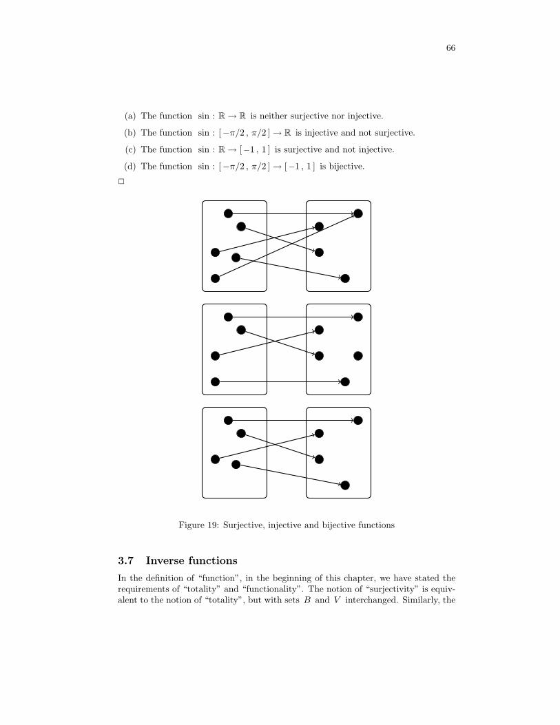
66

(a) The function sin : R→ R is neither surjective nor injective.

(b) The function sin : [−π/2 , π/2 ]→ R is injective and not surjective.

(c) The function sin : R→ [−1 , 1 ] is surjective and not injective.

(d) The function sin : [−π/2 , π/2 ]→ [−1 , 1 ] is bijective.

2

Figure 19: Surjective, injective and bijective functions

3.7 Inverse functions

In the definition of “function”, in the beginning of this chapter, we have stated therequirements of “totality” and “functionality”. The notion of “surjectivity” is equiv-alent to the notion of “totality”, but with sets B and V interchanged. Similarly, the

67

notion of “injectivity” is equivalent to the notion of “functionality”, but with B andV interchanged. Recall that for every relation R from B to V its transpositionRT is the relation from V to B defined by:

v RT b ⇔ bR v , for all b, v .

Function f being surjective now means that relation fT is total, and f being injec-tive means that relation fT is functional. From this we conclude immediately thatif f is bijective relation then fT is a function from V to B . This function happensto be f ’s inverse, and it is denoted by f−1 .

3.15 Definition. Function g in V →B is an inverse of function f in B→V if:

g f = IB ∧ f g = IV .

3.16 Lemma. A function has at most one inverse, that is, if g and h both are inversesof f , then g = h .

Proof. Assume that g and h both are inverses of f . Then

g = g IV = g (f h) = (g f) h = IB h = h.

Lemma 3.16 justifies to speak about ‘the’ inverse of a function rather than ‘an’inverse, and to fix the notation f−1 for it.

3.17 Lemma. Function g is the inverse of function f if and only if f is the inverse ofg .

Proof. Directly by definition.

3.18 Lemma. A function f has an inverse if and only if f is bijective.

Proof. First assume that f : B → V has an inverse g : V → B. Let y ∈ V , thenf(g(y)) = (f g)(y) = IV (y) = y, proving that f is surjective.

Assume that x, x′ ∈ B satisfy f(x) = f(x′). Then

x = IB(x) = (g f)(x) = g(f(x)) = g(f(x′)) = (g f)(x′) = IB(x′) = x′,

proving that f is injective. So f is bijective.Conversely, assume that f : B → V is bijective. Define g : V → B by defining

g(y) to be the unique element x ∈ B such that f(x) = y, for every y ∈ V . Theng(f(x)) = x and f(g(y)) = y for all x ∈ B and all y ∈ V , proving

g f = IB ∧ f g = IV ,

68

hence g is the inverse of f .

3.19 Lemma. If functions f in B→V and g in V →Z both are bijective then

(g f )−1 = f−1 g−1 .

2

Proof. We have to prove that f−1 g−1 is the inverse of g f . This follows from

(f−1 g−1) (g f) = f−1 (g−1 g) f = f−1 IV f = f−1 f = IB

and

(g f) (f−1 g−1) = g (f f−1) g−1 = g IV g−1 = g g−1 = IZ .

3.8 Finite sets and counting

The elements of finite sets can be counted. That is, we can define a function # , say,that maps every finite set to its number of elements. So, for finite set V its numberof elements #V is a natural number. We have that #V = n if and only if there is abijection from V to 1, 2, . . . , n.Without proof we collect some standard properties of # .

3.20 Properties. For all finite sets U, V and value v :

(0) #U = 0 ⇔ U = ø

(1) #v = 1

(2) 0 ≤ #U

(3) # (U ∪V ) = #U + #V − # (U ∩V )

(4) # (U ∪V ) ≤ #U + #V

(5) # (U ∪V ) = #U + #V , if U ∩V = ø

(6) #V = #U + # (V \U ) , if U ⊆V

(7) #U ≤ #V , if U ⊆V

(8) #U = #V ⇔ U = V , if U ⊆V

2

Notice that these properties are mutually dependent. For example, property (4)follows directly from (3) and (2) , property (5) is an instance of (3) , and (6) is aninstance of (5) , whereas (7) follows from (6) and (2) .

69

* * *

Functions on finite sets yield finite images. In what follows function f has typeB→V , where B and V are finite sets.

3.21 Lemma. # (f(B)) ≤ #B

Proof. By induction on the structure of B . If B = ø then f(B) = ø too, hence, inthis case we even have # (f(B)) = #B . If B = A∪b , for some b not in A wehave:

# (f (A∪b) )

= f over ∪ # (f(A)∪ f (b) )

≤ property 3.20 (4) # (f(A)) + # (f (b) )

= definition of f (b) # (f(A)) + # (f(b))

= property 3.20 (1) (twice) # (f(A)) + # (b)

≤ Induction Hypothesis #A + # (b)

= property 3.20 (5) , using ¬(b∈A) # (A∪b)

3.22 Lemma. “f is injective” ⇔ # (f(B)) = #B

Proof. By mutual implication.

“⇒ ”: Very similar to the proof of Lemma 3.21, using that # (f(A)∪ f (b) ) nowis equal to # (f(A)) + # (f (b) ) , because for injective f we have ¬(f(b)∈ f (A) )if ¬(b∈A) .

“⇐ ”: By contraposition, that is, if f is not injective then # (f(B)) 6= #B . If f isnot injective then B contains elements a, b , say, with a 6= b and f(a) = f(b) . Now:

# (f(B))

= a 6= b and f(a) = f(b), so f(B\a) = f(B) # (f(B\a))

≤ Lemma 3.21

70

# (B\a)= a∈B

#B − 1 ,

from which we conclude that # (f(B)) < #B , hence, also # (f(B)) 6= #B .

3.23 Lemma. “f is injective” ⇒ #B ≤ #V

Proof.#B

= f is injective: Lemma 3.22 # (f(B))

≤ f(B)⊆V : property 3.20 (7) #V

3.24 Lemma. “f is surjective” ⇒ #V ≤ #B

Proof.#V

= f is surjective: f(B) = V # (f(B))

≤ Lemma 3.21 #B

3.25 Lemma. “f is bijective” ⇒ #V = #B

Proof.Since f is injective, from Lemma 3.22 we conclude # (f(B)) = #B.Since f is surjective we conclude f(B) = V . So #V = #B.

Without further proofs we observe that the converses to the two latter lemmashold as well.

Properties.

(0) #B ≤ #V ⇒ (∃f : f ∈B→V : “f is injective” )

(1) #V ≤ #B ⇒ (∃f : f ∈B→V : “f is surjective” )

71

Now we are ready for the main theorem of this subsection.

3.26 Theorem. For f a function of type B→V , for finite sets B, V , and if #B = #V ,we have:

“f is injective” ⇔ “f is surjective”

Proof.“f is injective”

⇔ Lemma 3.22 # (f(B)) = #B

⇔ #B = #V # (f(B)) = #V

⇔ f(B)⊆V : property 3.20 (8) f(B) = V

⇔ Lemma 3.12 “f is surjective”

As a consequence of Theorem 3.26 we conclude that for functions from a finiteset to itself, the properties injectivity and surjectivity coincide. Here finiteness isessential. For instance, the function s : N→ N defined by s(x) = x+ 1 for all x ∈ Nis injective, but not surjective since no element maps to 0. Conversely, the functionf : N → N defined by f(x) = x − 1 for all x > 0, and f(0) = 0 is surjective, but notinjective since f(0) = 0 = f(1).

3.27 Example. Suppose p and q are two different prime numbers. We consider thefunction ϕ in [ 0 . . p )→ [ 0 . . p ) , defined by ϕ(x) = (x ∗ q) mod p , for all x∈ [ 0 . . p ) .

We prove that ϕ is a bijection. By Theorem 3.26 it suffices to show that ϕ isinjective. To this end we derive, for x, y ∈ [ 0 . . p ) :

ϕ(x) = ϕ(y)

⇔ definition of ϕ (x ∗ q) mod p = (y ∗ q) mod p

⇔ property of mod ( (x−y) ∗ q ) mod p = 0

⇔ property of mod and | p | ( (x−y) ∗ q )

⇔ “p is prime”: (p | ) distributes over ∗

72

p | (x−y) ∨ p | q⇔ “p and q are prime” and p 6= q , hence : ¬(p | q)

p | (x−y)

⇔ x, y ∈ [ 0 . . p ) , hence −p< x−y < p x = y .

2

3.9 Exercises

1. Set A is given by A = 1 , 2 , 3 , 4. Which of the following relations are func-tions from A to A ?

(a) (1, 3), (2, 4), (3, 1), (4, 2);(b) (1, 3), (2, 4);(c) (1, 1), (2, 2), (3, 3), (4, 4), (1, 3), (2, 4), (3, 1), (4, 2);(d) (1, 1), (2, 2), (3, 3), (4, 4).

2. Suppose f and g are functions from R to R defined by f(x) = x2 and g(x) = x+1for all x ∈ R. What is g f and what is f g?

3. Which of the following functions from 1, 2, 3, 4 to a, b, c, d is injective, sur-jective and/or bijective?

(a) (1, a), (2, d), (3, c), (4, b).(b) (1, b), (2, d), (3, c), (4, b).(c) (1, d), (2, b), (3, a), (4, c).(d) (1, c), (2, d), (3, c), (4, b).

For the bijective functions determine their inverses.

4. Which of the following functions is injective, surjective and/or bijective?

(a) f : R→ R, f(x) = x2 for all x ∈ R.

(b) f : R→ R≥0, f(x) = x2 for all x ∈ R.

(c) f : R≥0 → R≥0, f(x) = x2 for all x ∈ R.

5. Suppose R and S are relations on a set V with R ;S = I and S ;R = I .Prove that both R and S are bijective functions.

6. Let R be a finite relation with adjacency matrix A . Prove the following state-ments:

(a) If every row of A contains exactly one non-zero entry, then R is a function.

73

(b) If, in addition, every column of A contains at most one entry, then functionR is injective.

(c) If every row and column of A contain exactly one 1 , then R is a bijection.What is the adjacency matrix of the inverse function?

7. Let B and V be sets and let R be a relation from B to V . Then, for everyv∈V , we have defined5 the pre-image of v as the set R[v ] , thus:

R[v ] = b∈B | bRv ,

which, obviously, is a subset of B .

(a) Prove that the relation (v , R[v ]) | v∈V is a function from V to P(B)(the set of all subsets of B ).

(b) Prove that, if F is a function in V →P(B) , then the set RF definedby RF = (b, v) | b∈F (v) ∧ v∈V is a relation from B to V , withRF

[v ] = F (v) , for all v∈V .

8. Given are two bijective functions f , of type U→V , and g , of type V →W .Prove that: (g f )−1 = f−1 g−1 .

9. We consider functions f, g, h , of type U→U , such that both gf and hgare bijective. Prove that hgf is bijective as well.

10. Prove that an injective function f in B→V has a partial inverse, that is, apartial function g from V to B such that g f = IB . What is the domain ofg ?

11. (a) Give an example of a set A and a surjective function f : A→ A for whichf(a) = f(b) for some a, b ∈ A, a 6= b.

(b) Prove that this is not possible if A is finite.

12. Let f, g : A→ A for a finite set A for which f g is injective. Prove that bothf and g are surjective.

13. (a) Give an example of two sets A ⊆ B and an injective function f : B → Asuch that A 6= B.

(b) Prove that, if A ⊆ B are finite sets and f : B → A is injective, then A = B.

14. (a) Give an example of a set A and functions f, g : A→ A such that f g = I,but for which no h : A→ A exists such that h f = I.

(b) Prove that this is not possible for A finite.

5See the chapter on relations.

74

4 Posets and lattices

4.1 Partial orders

Many important relations cover some idea of greater and smaller: the partial orders.

4.1 Definition. An (endo)relation v (“under”) on a set P is called a partial order ifit is reflexive, antisymmetric, and transitive. We recall that this means that, for allx, y, z∈P , we have:

• xv x ;

• xv y ∧ y v x ⇒ x= y ;

• xv y ∧ y v z ⇒ xv z .

The pair (P, v ) is called a partially ordered set or, for short, a poset .Two elements x and y in a poset (P, v ) are called comparable if xvy or yvx ,

otherwise they are called incomparable, that is, if ¬(xvy) and ¬(yvx) .A partial order is a total order , also called linear order , if every two elements are

comparable.2

4.2 Lemma. For every poset (P, v ) and for every subset X of P , the pair (X, v ) isa poset too.2

4.3 Example.

• On every set, the identity relation I is a partial order. It is the smallest possiblepartial order relation on that set.

• On the real numbers R the relation ≤ is a total order: every two numbersx, y∈R satisfy x≤ y or y≤x . Restriction of ≤ to any subset of R – forexample, restriction to Q,Z,N – also yields a total order on that subset.

• The power set P(V ) of a set V , that is, the set of all subsets of V , withrelation ⊆ (subset inclusion), is a poset. This P contains a smallest element,namely ø , and a largest element, namely V itself. For #V ≥ 2 the order isnot total: if u, v are distinct then neither u ⊆ v nor v ⊆ u, so u andv are incomparable.

• The relation | (“divides”) is a partial order on the positive naturals, definedby

x | y ⇔ (∃z : z ∈ N : x ∗ z = y).

This order is not total, for instance, 2 and 3 are incomparable.

75

2

4.4 Definition. The irreflexive part of a partial order relation v is denoted by <

(“strictly under”) and is defined by, for all x, y∈P :

x< y ⇔ xvy ∧ x 6= y .

2It is straightforward to prove that the relation < is irreflexive, antisymmetric

and transitive. Further, it directly follows from the definition that for all x, y∈P :xv y ⇔ x<y ∨ x= y .

4.5 Lemma. If (P, v ) is a poset, then the corresponding directed graph, with vertexset P and arrows (x, y) whenever x<y , is acyclic.2

If we want to draw a picture of a finite poset, with the greater elements on topand the smaller elements below, and an arrow from x to y if x v y holds, we usuallydo not draw the whole graph. Edges from a node x to itself, representing x v x arenot drawn, and an edge from x to y with x v y is only drawn if there is no z, distinctfrom both x and y, for which we have x v z and z v y. The resulting directed graph iscalled the Hasse diagram for (P,v), named after the German mathematician HelmutHasse (1898-1979). Hasse diagrams are drawn in such a way that two vertexes x andy with x v y are connected by an edge going upwards. In Theorem 4.14 we will seethat this is always possible. Consequently, the edges in Hasse diagrams do not needan arrow point to indicate the direction. For example the Hasse diagram for the poset(P(a , b , c) ,⊆) is drawn as in Figure 20.

The Hasse diagram is a relation itself, on the same finite set P . In fact, it isthe smallest relation H of which the reflexive transitive closure H∗ coincides with thegiven relation v.

* * *

There are various ways of constructing new posets out of old ones. We discuss someof them. In the sequel both (P, v ) and (Q, v ) are posets. Notice that we usethe same symbol, v , for the two different partial order relations on sets P andQ . If confusion may arise we distinguish the two relations by using vP and vQ ,respectively.

• As already stated in Lemma 4.2, for every subset X of P the pair (X, v )is a poset, with relation v restricted to X . Thus restricted v is called theinduced order on X .

• Relation w (“above”), defined by, for all x, y∈P , xwy ⇔ yvx is a partialorder too, called the dual order to v ; hence, (P, w ) also is a poset.

• Let V be a set. On the set V →P of functions from V to P we can define apartial order vVP , say, as follows, for all f, g ∈ V →P :

76

a, b, c

a, ca, b b, c

ba c

ø

Figure 20: A Hasse diagram of (P(a, b, c) , ⊆ )

f vVP g ⇔ (∀v : v∈V : f(v) vP g(v) ) .

Then (V →P , vVP ) is a poset.

• On the Cartesian product P×Q we can define a partial order as follows. For(p, q) , (x, y) ∈ P×Q we define:

(p, q) v (x, y) ⇔ p vP x ∧ q vQ y .

Thus defined relation v is a partial order, called the product order on P×Q .

• On the Cartesian product P×Q we also can define a partial order as follows.For (p, q) , (x, y) ∈ P×Q we define:

(p, q) v (x, y) ⇔ (p 6=x ∧ p vP x ) ∨ (p=x ∧ q vQ y ) .

This relation v is a partial order too, called the lexicographic order on P×Q .

The notions of product order and lexicographic order can be extended to (finite)products of more than two sets.

A poset’s structure is determined by its partial order relation, as denoted by v in theprevious section. Sometimes we wish to prove equalities in a poset, and then it canbe convenient if we can reformulate an equality in terms of the partial order relation:that enables us to reason in terms of the partial order.

77

The following lemma provides such a connection between equality and the partialorder, apart from the property x = y⇔(xvy ∧ yvx) that holds by reflexivity andanti-symmetry.

4.6 Lemma. In every poset (P, v ) we have, for all x, y ∈P :

(a) x = y ⇔ (∀z : z∈P : xvz ⇔ yvz ) ;

(b) x = y ⇔ (∀z : z∈P : zvx ⇔ zvy ) .

Proof. We prove (a) only; the proof of (b) follows, mutatis mutandis, the same pat-tern. We do so by mutual implication.

“⇒ ”: Assuming x= y we may substitute x for y and vice versa wherever we like; inparticular, if we substitute x for y in our demonstrandum (∀z : z∈P : xvz ⇔ yvz ) ,we obtain (∀z : z∈P : yvz ⇔ yvz ) , which is true because of the reflexivity of ⇔ .

“⇐ ”: Assuming (∀z : z∈P : xvz ⇔ yvz ) , by the instantiation z := x we obtainxv x ⇔ y v x , which is equivalent to y v x , because v is reflexive. Moreover, bythe instantiation z := y we obtain xv y ⇔ y v y , which is equivalent to xv y . Bythe antisymmetry of v we conclude x= y , as required.

4.2 Extreme elements

4.7 Definition. For any subset X of a poset (P, v ) we define, for all m∈P :

(a) m is X ’s maximum, or largest element if:

m∈X ∧ (∀x : x∈X : xvm ) .

(b) m is X ’s minimum, or least element if:

m∈X ∧ (∀x : x∈X : mvx ) .

(c) m is a maximal element of X if:

m∈X ∧ (∀x : x∈X : ¬ (m<x) ) .

(d) m is a minimal element of X if:

m∈X ∧ (∀x : x∈X : ¬ (x<m) ) .

2

Note that by definition ¬(m<x) is equivalent to mvx ⇒ x = m, so maximalityof m can be reformulated as m∈X ∧ (∀x : x∈X : mvx ⇒ x = m) , and similarfor minimality.

Notice the difference between the notions “maximum” and “maximal”. A valuem∈P is X ’s maximum if m∈X and all elements in X are under m , whereas mis a maximal element of X if m∈X and X contains no elements strictly above m .

78

A subset of a partially ordered set does not necessarily contain such extremeelements. The next lemma states that if it exists, however, the maximum of a subsetis unique, and so is the minimum, if it exists. If subset X has a maximum we denoteit by maxX , and its minimum we denote by minX .

4.8 Lemma. Let X be a subset of a poset (P, v ) . If m and n both are X ’s maximumthen m=n . If m and n both are X ’s minimum then m=n .2

Proof. Assume that both m and n are a maximum of X, then by definition m,n ∈ Xand (∀x : x ∈ X : xvm ∧ xvn). So we both have nvm and mvn. Since v isanti-symmetric we conclude m = n.

A subset of a partially ordered set does not necessarily contain maximal or mini-mal elements. Such elements are not unique either: a subset may have many maximalor minimal elements. As a rather trivial example, consider poset (P, IP ) , where theidentity relation IP is the smallest possible partial order on P: x IP y ⇔ x= y . Withthis particular order all elements of a subset X⊆P both are maximal and minimal.

4.9 Definition. Let (P, v ) be a poset. If the whole set P has a minimum this isoften denoted by ⊥ (“bottom”), and if P has a maximum this is often denoted by> (“top”). If P has a minimum the minimal elements of P \⊥ are called P ’satoms.

4.10 Example.

• If we consider the poset of all subsets of a set V , then the empty set ø is theminimum of the poset, whereas the whole set V is the maximum. The atomsare the subsets of V containing just a single element.

• In the poset (N+, | ) the whole set, N+ , has no maximum. Its minimum,however, equals 1 . The atoms are the prime numbers. Surprisingly, in the poset(N, | ) the whole set N has a maximum: the element 0, since by definitionevery number is a divisor of 0.

• If (P, v ) is totally ordered then subset x , y has a maximum and a minimum,for all x, y ∈P .

2

4.11 Lemma. In a poset (P, v ) for every subset X its maximum, if it exists, is a maximalelement of X ; also, its minimum, if it exists, is a minimal element of X .

Proof. Assume m is the maximum of X. Then m ∈ X and xvm for all x ∈ X.Choose x ∈ X satisfying mvx. Then using antisymmetry and xvm we concludex = m, so proving mvx ⇒ x = m. This proves that m is maximal.

The proof for minimal/minimum is similar.

79

4.12 Lemma. If a poset (P, v ) is a total order then every subset X⊆P has at most onemaximal element, which then also is its maximum. Also, X has at most one minimalelement, which then also is its minimum.

Proof. Assume that m is maximal in X and n ∈ X. Then by definition ¬(m<n), som = n or ¬(mvn). If ¬(mvn) then from totality we conclude nvm. So in bothcases we have nvm. This proves that m is the maximum of X. If moreover n ismaximal too, we similarly prove nvm, so by antisymmetry we conclude m = n.

The proof for minimal/minimum is similar.

4.13 Lemma. Let (P, v ) be a nonempty and finite poset. Then P contains a maximalelement and a minimal element.Proof. Choose x1 ∈ P arbitrary. For i = 1, 2, 3, . . . choose xi+1 such that xi <xi+1,that is, xivxi+1 and xi 6= xi+1. If at some point no such xi+1 exists, we have founda maximal element xi.

Otherwise, the process goes on forever yielding an infinite sequence

x1 <x2 <x3 <x4 <x5 < · · · .

Since P is finite, not all xi can be distinct, so there is some i < j such that xi = xj .So xiv∗xj−ivxj = xi. For a transitive relation R one easily proves by inductionRn ⊆ R for n > 0. So if i < j − 1 then xivxj−1. If i = j − 1 then xi = xj−i, soin all cases we conclude xivxj−1. So xivxj−1vxj = xi. Now antisymmetry yieldsxj−1 = xj , contradicting the requirement xi 6= xi+1 in the construction for all i.

4.14 Theorem. [ Topological sorting ] For any finite poset (P, v ) with #P = n thereexists a bijection f : P → 1, 2, . . . , n such that x<y⇒f(x) < f(y) for all x, y ∈ P .

Proof. We prove the theorem by induction on n = #P . For n = 1 we definef(x) = 1 for the single element x of P . It is clearly a bijection, and the other propertyholds since x<y never occurs.

For n > 1 we choose p ∈ P such that p is maximal in P ; this is possible byLemma 4.13. By the induction hypothesis there exists f ′ : P \ p → 1, . . . , n − 1such that f ′(x) < f ′(y) for all x, y ∈ P \ p. Next we define f : P → 1, . . . , nby f(p) = n and f(x) = f ′(x) for x 6= p. It is surjective since f ′ is surjective andf(p) = n; bijectivity follows from Theorem 3.26.

It remains to prove that f(x) < f(y) for all x, y ∈ P satisfying x<y, which wedo by case analysis:

• x = p does not occur since x<y contradicts maximality of x = p,

• if y = p then x ∈ P \ p, so

f(x) = f ′(x) ≤ n− 1 < n = f(p) = f(y),

80

• if x 6= p 6= y then f(x) = f ′(x) < f ′(y) = f(y).

Topological sorting justifies the existence of Hasse diagrams: if every node x isdrawn on height f(x), then for every x<y the element y is drawn higher than x.

4.15 Example. Topological sorting has various applications. For example consider a (so-called) spreadsheet . In a spreadsheet the values in various cells depend on each other,but, in a correct spreadsheet, in an acyclic way only. The value in any particular cell inthe spreadsheet can only be computed if the values in all cells on which this particularcell depends have been computed already. Therefore, an efficient implementation ofthese computations requires that they are performed in the “right” order. This givesrise to a partial order on the set of cells within a spreadsheet. By topological sortingthe set of cells can be linearized in such a way that every cell precedes all cellsdepending on it; thus the computations of the values in the cells can be performed ina linear order.

4.3 Upper and lower bounds

4.16 Definition. For any subset X of a poset (P, v ) we define, for all m∈P :

(a) m is an upper bound of X if: (∀x : x∈X : xvm )

(b) m is a lower bound of X if: (∀x : x∈X : mvx )

2

4.17 Properties.

(a) If P has a maximum > then > is an upper bound of every subset of P .

(b) If P has a minimum ⊥ then ⊥ is a lower bound of every subset of P .

(c) Every element in P is an upper bound and a lower bound of ø .

(d) If it exists maxX is an upper bound of X , for all X⊆P .

(e) If it exists minX is a lower bound of X , for all X⊆P .

2

For any subset X⊆P we can consider the set m∈P | (∀x : x∈X : xvm ) of all upper bounds of X . This set may or may not have a minimum. If it has aminimum, this minimum is called the supremum of X , notation supX . Alternatively,it is sometimes also called X ’s least upper bound , notation lubX .

Similarly, we can consider the set m∈P | (∀x : x∈X : mvx ) of all lowerbounds of X . This set may or may not have a maximum. If it has a maximum, this

81

maximum is called the infimum of X , notation infX . Alternatively, it is sometimesalso called X ’s greatest lower bound , notation glbX .

By combination of the definitions of maximum/minimum and of upper/lowerbounds we can define supremum and infimum in a more direct way.

4.18 Definition. For any subset X of a poset (P, v ) we define, for all m∈P :

(a) m is X ’s supremum if both:

(∀x : x∈X : xvm ) , and:

(∀x : x∈X : xvz ) ⇒ mv z , for all z∈P .

Notice that the first requirement expresses that m is an upper bound of X ,and that the second one expresses that m is under all upper bounds of X .

(b) m is X ’s infimum if both:

(∀x : x∈X : mvx ) , and:

(∀x : x∈X : zvx ) ⇒ z vm , for all z∈P .

2

4.19 Example.

• For a set V its power set P(V ) – the set of all subsets of V – with relation ⊆ is a

poset, and any subset X of P(V ) has a supremum, namely (⋃

U :U∈X U ) ,and

an infimum, namely (⋂

U :U∈X U ) .

• The set N+ of positive natural numbers with relation | (“divides”) is a poset.The supremum of two elements a, b∈N+ is their least common multiple, thatis, the smallest of all positive naturals m satisfying a|m and b|m ; usually,this value is denoted by lcm(a, b) .

Similarly, the greatest common divisor of a and b , denoted by gcd(a, b) , isthe infimum of a , b .

2

4.20 Lemma. For poset (P, v ) and for p∈P we have: supp = p and infp = p .

Proof. By Definition 4.18, to prove supp = p we must prove:

(∀x : x∈p : xvp )

⇔ definition of p (∀x : x= p : xvp )

⇔ 1-pt. rule p v p

⇔ v is reflexive

82

true ,

and, for all z∈P :

(∀x : x∈p : xvz )

⇔ same steps as above p v z ,

which is the desired result.

4.21 Lemma. Let (P, v ) be a poset and X ⊆ P .

(a) If X has a maximum m, then supX = m.

(b) If supX ∈ X, then supX is the maximum of X.

(c) If X has a minimum m, then infX = m.

(d) If infX ∈ X, then infX is the minimum of X.

Proof.

(a) We have to prove that m satisfies the defining properties of supX. The first isthat supX is an upper bound, which follows from the definition of maximum.For the second assume that x is an upper bound of X, we have to prove thatmvx. This follows from the fact that m ∈ X and the definition of upper bound.

(b) Immediate from the definitions.

(c) Similar to (a).

(d) Immediate from the definitions.

An important difference between supremum and maximum of a set is that a set’ssupremum may or may not be an element of that set, whereas a set’s maximum alwaysis an element of that set. The above lemma states, however, that if a set’s supremumis in that set, then this supremum also is the set’s maximum.

The following lemma provides a different but equivalent characterization of supre-mum and infimum that occasionally turns out to be very useful.

4.22 Lemma. Let X be a subset of a poset (P, v ) . For m∈P we have:

(a) m is X ’s supremum if and only if:

(∀z : z∈P : mv z ⇔ (∀x : x∈X : xvz ) ) .

(b) m is X ’s infimum if and only if:

(∀z : z∈P : z vm ⇔ (∀x : x∈X : zvx ) ) .

83

Proof. We prove (a) only; the proof for (b) follows, mutatis mutandis, the same pat-tern. Firstly, we let m be X ’s supremum according to Definition 4.18. Then, forz∈P we prove the equivalence of mv z and (∀x : x∈X : xvz ) , by “cyclic implica-tion”:

m v z

⇔ Definition 4.18: m is an upper bound of X (∀x : x∈X : xvm ) ∧ m v z

⇒ ∀ introduction (∀x : x∈X : xvm ) ∧ (∀x : x∈X : mvz )

⇔ combining terms (∀x : x∈X : xvm ∧ mvz )

⇒ v is transitive (∀x : x∈X : xvz )

⇒ Definition 4.18: m is under all upper bounds m v z .

Secondly, let m satisfy:

(2) (∀z : z∈P : mv z ⇔ (∀x : x∈X : xvz ) ) .

Then we must prove that m is X ’s supremum. Well, m is an upper bound:

(∀x : x∈X : xvm )

⇔ (2) , with z := m m vm

⇔ v is reflexive true ,

and that m is under all upper bounds follows directly from (2) , because ⇔ isstronger than ⇒ .

4.23 Properties.

(a) If P has a maximum > then > = supP and > = inf ø .

(b) If P has a minimum ⊥ then ⊥ = infP and ⊥ = sup ø .

2

84

4.4 Lattices

4.4.1 Definition

In the previous section we have introduced the notions of supremum – least upperbound – and infimum – greatest lower bound – of subsets of a poset. Generally, such asubset does not always have a supremum or an infimum, just as, generally, not everysubset has a maximum or a minimum. (Recall Lemma 4.21, for the relation betweensupremum and maximum, and between infimum and minimum, respectively.)

Partially ordered sets in which particular subsets do have suprema and/or infimaare of interest, in particular “lattices” and “complete lattices”.

4.24 Definition. A poset (P, v ) is a lattice, if for all x, y ∈P the subset x , y has asupremum and an infimum. Because this pertains to two-element sets, it is customaryto use infix-notation to denote their suprema and infima. For these purposes binaryoperators t (“cup”) and u (“cap”) are used: the supremum of x , y then iswritten as x t y and its infimum as x u y .2

4.25 Example. Here are some examples of lattices we already encountered before.

• (R, ≤) is a lattice. For x, y ∈R we have: x t y = xmax y and x u y = xmin y .

• For a set V the poset (P(V ) , ⊆ ) is a lattice, with t = ∪ and u = ∩ .

• The poset (N+ , | ) is a lattice, with a t b = lcm(a, b) , the least common mulit-ple, and a u b = gcd(a, b) , the greatest common divisor.

2

The following lemma actually is a special case of Lemma 4.22, namely for non-empty subsets with at most two elements; that is, this is Lemma 4.22 with X := x , y .

4.26 Lemma. In every lattice (P, v ) we have, for all x, y, z ∈P :

(a) x t y v z ⇔ x v z ∧ y v z ;

(b) z v x u y ⇔ z v x ∧ z v y .

2

Actually, this lemma can serve as an alternative definition of t and u , as theoriginal definition follows from it. As a special case, we obtain the following lemma,expressing that x t y is an upper bound and that x u y is a lower bound.

4.27 Lemma. In every lattice (P, v ) we have, for all x, y ∈P :

(a) x v x t y ∧ y v x t y ;

(b) x u y v x ∧ x u y v y .

85

Proof. Instantiate Lemma 4.26 with z := x t y and z := x u y , respectively.

4.28 Lemma. In every lattice (P, v ) we have, for all x, y ∈P :

(a) x v y ⇔ x t y = y ;

(b) x v y ⇔ x u y = x .

Proof. We prove (a) only, by calculation:

x t y = y

⇔ v is reflexive and antisymmetric x t y v y ∧ y v x t y

⇔ x t y is an upper bound of y x t y v y

⇔ Lemma 4.26 , with z := y x v y ∧ y v y

⇔ v is reflexive x v y

4.4.2 Algebraic properties

The lattice operators have interesting algebraic properties, as reflected by the follow-ing theorem.

4.29 Theorem. Let (P, v ) be a lattice. Then for all x, y, z ∈P we have:

(a) x t x = x and x u x = x : t and u are idempotent ;

(b) x t y = y t x and x u y = y u x : t and u are commutative;

(c) x t (y t z) = (x t y) t z and x u (y u z) = (x u y) u z : t and u are

associative;

(d) x t (x u y) = x and x u (x t y) = x : absorption.

Proof.

(a) See Lemma 4.20.

(b) By symmetry: set x , y equals set y , x .

(c) By (Lemma 4.6), for all w∈P :

86

x t (y t z) v w

⇔ Lemma 4.26 x v w ∧ y t z v w

⇔ Lemma 4.26 x v w ∧ y v w ∧ z v w

⇔ Lemma 4.26 x t y v w ∧ z v w

⇔ Lemma 4.26 (x t y) t z v w .

(d) We prove x t (x u y) = x only, by calculation:

x t (x u y) = x

⇔ Lemma 4.28 x u y v x

⇔ x u y is a lower bound of x true .

Conversely, the following theorem expresses that every structure with operatorshaving the above algebraic properties “is” – can be extended into – a lattice.

4.30 Theorem. Let P be a set with two binary operators t and u ; that is, theseoperators have type P×P → P . Let these operators have algebraic properties (a)through (d), as in the previous theorem. Then the relation v , on P and defined byxv y ⇔ x t y = y for all x, y ∈P , is a partial order, and (P, v ) is a lattice.2

A direct consequence of Theorem 4.29, particularly of the associativity of theoperators, is that every finite and non-empty subset of a lattice has a supremum andan infimum. Notice that the requirement “non-empty” is essential here: in a latticethe empty set may not have a supremum or infimum.

4.31 Theorem. Let (P, v ) be a lattice. Then every finite and non-empty subset of Phas a supremum and an infimum.

Proof. By Mathematical Induction on the size of the subsets, and using Theorem 4.29.

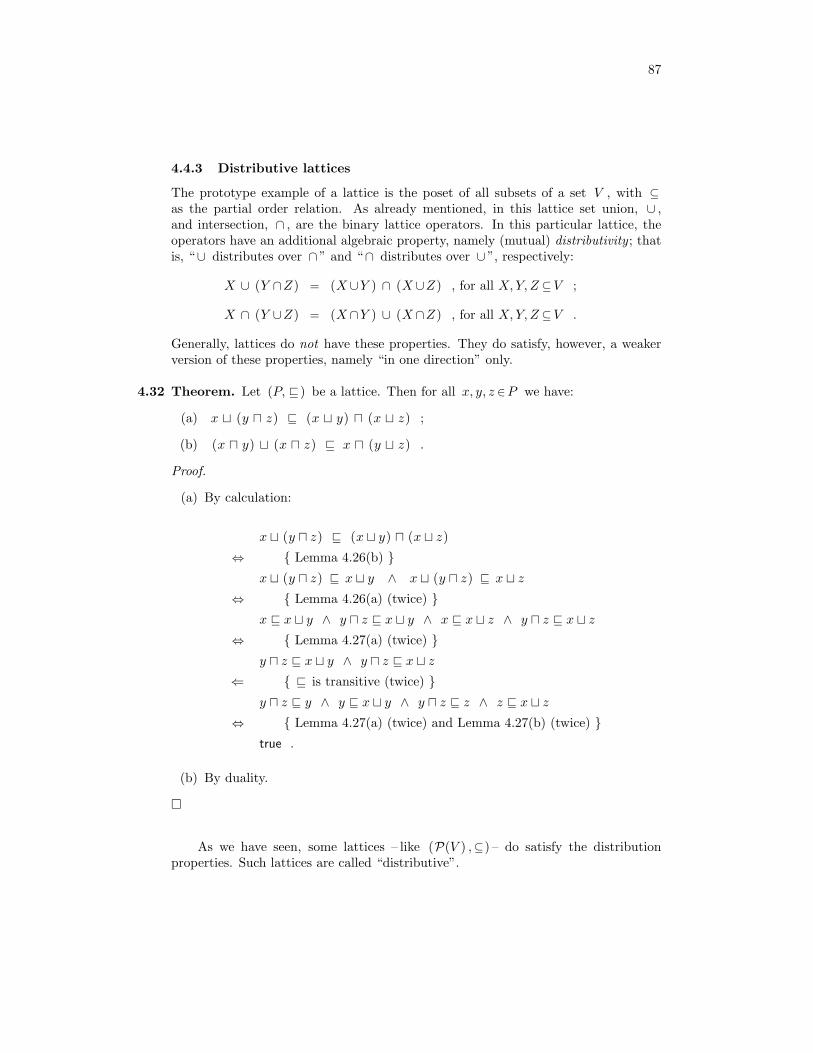
87

4.4.3 Distributive lattices

The prototype example of a lattice is the poset of all subsets of a set V , with ⊆as the partial order relation. As already mentioned, in this lattice set union, ∪ ,and intersection, ∩ , are the binary lattice operators. In this particular lattice, theoperators have an additional algebraic property, namely (mutual) distributivity ; thatis, “∪ distributes over ∩ ” and “∩ distributes over ∪ ”, respectively:

X ∪ (Y ∩Z) = (X∪Y ) ∩ (X∪Z) , for all X,Y, Z ⊆V ;

X ∩ (Y ∪Z) = (X∩Y ) ∪ (X∩Z) , for all X,Y, Z ⊆V .

Generally, lattices do not have these properties. They do satisfy, however, a weakerversion of these properties, namely “in one direction” only.

4.32 Theorem. Let (P, v ) be a lattice. Then for all x, y, z ∈P we have:

(a) x t (y u z) v (x t y) u (x t z) ;

(b) (x u y) t (x u z) v x u (y t z) .

Proof.

(a) By calculation:

x t (y u z) v (x t y) u (x t z)

⇔ Lemma 4.26(b) x t (y u z) v x t y ∧ x t (y u z) v x t z

⇔ Lemma 4.26(a) (twice) x v x t y ∧ y u z v x t y ∧ x v x t z ∧ y u z v x t z

⇔ Lemma 4.27(a) (twice) y u z v x t y ∧ y u z v x t z

⇐ v is transitive (twice) y u z v y ∧ y v x t y ∧ y u z v z ∧ z v x t z

⇔ Lemma 4.27(a) (twice) and Lemma 4.27(b) (twice) true .

(b) By duality.

As we have seen, some lattices – like (P(V ) ,⊆) – do satisfy the distributionproperties. Such lattices are called “distributive”.

88

4.33 Definition. A distributive lattice is a lattice (P, v ) in which t and u distributeover each other; that is, for all x, y, z ∈P :

(a) x t (y u z) = (x t y) u (x t z) ;

(b) x u (y t z) = (x u y) t (x u z) .

2

4.34 Example. Not every lattice is distributive. The smallest example illustrating this has5 elements >, a, b, c,⊥ , say, with this partial order: ⊥ is under all elements, a, b, care under > and are mutually incomparable. (See the Hasse diagram in Figure 21.)In this lattice a t (b u c) = a whereas (a t b) u (a t c) = > .

>

a b c

⊥

Figure 21: The smallest non-distributive lattice

4.4.4 Complete lattices

4.35 Definition. A complete lattice is a partial order in which every subset has a supre-mum and an infimum. In particular, the whole set has a supremum and an infimum,usually denoted by > and ⊥ , respectively. Notice that > and ⊥ also are the lat-tice’s maximum and minimum. (Recall Property 4.23.)2In computer science complete lattices are often used to give precise definitions ofseveral concepts, like semantics of a programming language. A key result that we donot present here is that in a complete lattice every monotone fucntion f : P → P ,that is, x v y ⇒ f(x) v f(y), has a least fixed point, that is, x | f(x) = x has aminimum.

4.36 Lemma. Every finite lattice is complete.

Proof. Let (P, v ) be a finite lattice. By Theorem 4.31 this lattice is almost completealready: every non-empty subset has a supremum and an infimum, so all we must dois prove that ø has a supremum and an infimum. From Property 4.23 we know that

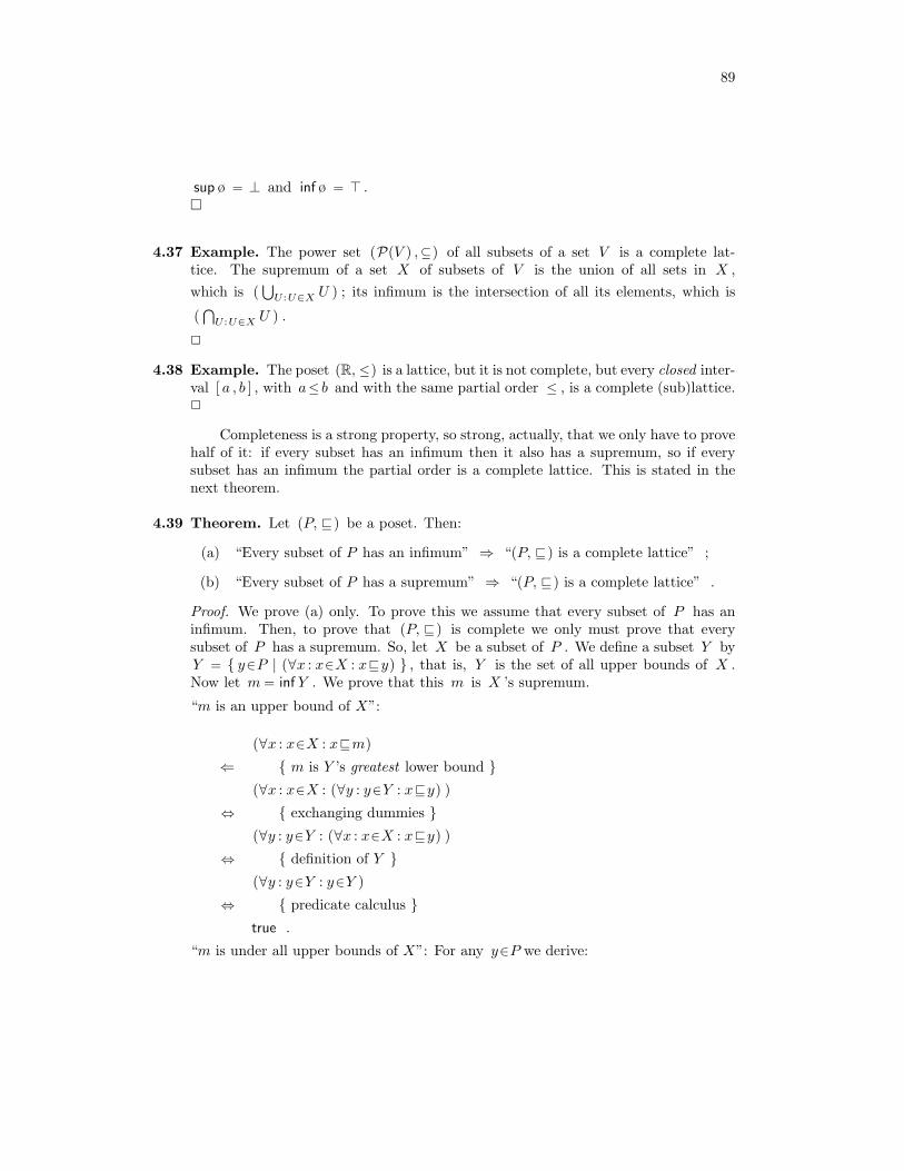
89

sup ø = ⊥ and inf ø = > .

4.37 Example. The power set (P(V ) ,⊆) of all subsets of a set V is a complete lat-tice. The supremum of a set X of subsets of V is the union of all sets in X ,which is (

⋃U :U∈X U ) ; its infimum is the intersection of all its elements, which is

(⋂

U :U∈X U ) .

2

4.38 Example. The poset (R, ≤) is a lattice, but it is not complete, but every closed inter-val [ a , b ] , with a≤ b and with the same partial order ≤ , is a complete (sub)lattice.2

Completeness is a strong property, so strong, actually, that we only have to provehalf of it: if every subset has an infimum then it also has a supremum, so if everysubset has an infimum the partial order is a complete lattice. This is stated in thenext theorem.

4.39 Theorem. Let (P, v ) be a poset. Then:

(a) “Every subset of P has an infimum” ⇒ “(P, v ) is a complete lattice” ;

(b) “Every subset of P has a supremum” ⇒ “(P, v ) is a complete lattice” .

Proof. We prove (a) only. To prove this we assume that every subset of P has aninfimum. Then, to prove that (P, v ) is complete we only must prove that everysubset of P has a supremum. So, let X be a subset of P . We define a subset Y byY = y∈P | (∀x : x∈X : xvy) , that is, Y is the set of all upper bounds of X .Now let m = inf Y . We prove that this m is X ’s supremum.

“m is an upper bound of X”:

(∀x : x∈X : xvm)

⇐ m is Y ’s greatest lower bound (∀x : x∈X : (∀y : y∈Y : xvy) )

⇔ exchanging dummies (∀y : y∈Y : (∀x : x∈X : xvy) )

⇔ definition of Y (∀y : y∈Y : y∈Y )

⇔ predicate calculus true .

“m is under all upper bounds of X”: For any y∈P we derive:

90

(∀x : x∈X : xvy)

⇔ definition of Y y ∈Y

⇒ m is a lower bound of Y m v y .

remark: In the proof of this theorem we introduced set Y as the set of all upperbounds of X . It is possible that X has no upper bounds, in which case Yis empty . This is harmless, because if every subset has an infimum then sohas the empty set. Thus, this proof crucially depends on the property thatalso the empty set has an infimum. Recall that in a non-complete lattice theempty set does not need to have an infimum or supremum. (Also see thediscussion preceding Theorem 4.31.)

2

4.5 Exercises

1. Consider the poset (N+, | ) . Let A = 3, 4, 5, 6, 7, 8, 9, 10, 11, 12.

(a) Establish all minimal and maximal elements of A.

(b) Give a subset of four elements of A that has a maximum.

(c) Give a subset of four elements of A that has a minimum.

2. Give an example of a poset that has exactly one maximal element, but not amaximum element.

3. Draw the Hasse diagram of

X ⊆ 1, 2, 3, 4 | 2 ∈ X ∨ 3 6∈ X

with respect to the partial order ⊆.

4. Let (P, v ) be a poset. Recall that for all x, y∈P :

x< y ⇔ xvy ∧ x 6= y .

Prove that the relation < is irreflexive, antisymmetric, and transitive.

5. Let (P, v ) be a poset. Prove that for all x, y ∈P :

(a) x v y ⇔ (∀z : z∈P : xvz ⇐ yvz ) ;

(b) x v y ⇔ (∀z : z∈P : zvx ⇒ zvy ) .

91

6. Let (P, v ) be a poset and X a subset of P . Prove that an element m∈X ismaximal if and only if for all x∈X we have mvx ⇒ m= x .

7. A poset (U,v) is given with two subsets X and Y for which sup(X) and sup(Y )exist, and sup(X) ∈ Y . Prove that sup(Y ) is an upper bound of X.

8. Let (U,v) be a poset and f : U → U a function. Define the relation ≤ on U by

x ≤ y ⇐⇒ f(x) v f(y).

(a) Prove that (U,≤) is a poset if f is injective.

(b) Give an example of a poset (U,v) and a non-injective function f : U → Usuch that (U,≤) is not a poset.

9. Consider the poset (N+, | ) .

(a) Establish the supremum and the infimum of 1, 2, 3, 4, 5.(b) Establish the supremum and the infimum of 1, 2, 3, 4, 6, 12.(c) Establish the supremum and the infimum of 3, 4, 5, 15, 20, 60.(d) Establish the supremum and the infimum of 3, 4, 5, 12.(e) Establish the supremum and the infimum of the set of all even numbers.

For all set also establish whether the set has a minimum and/or a maximum.

10. Let (U,v) be a poset. Two sets A,B ⊆ U are given, for which sup(A) exists,and for which b ∈ B is minimal in B and sup(A) v b. Prove that A ∩B ⊆ b.

11. Let (P, v ) be a lattice and x, y, z ∈P . Prove that:

(a) x v y ⇒ x t z v y t z ;

(b) x v z ⇒ z t (x u y) = z .

12. We consider the poset (Q , ≤) .

(a) Prove that the set x∈Q | x< 1 has no maximum.

(b) Prove that this set has a supremum.

13. We consider a poset (P, v ) ; let X and Y be subsets of P such that supXand inf Y both exist. In addition it is given that xv y , for all x∈X and y∈Y .Prove that supX v inf Y .

14. We consider a poset (P, v ) ; let X be a subset of P .

(a) Prove that if X contains two (different) maximal elements then X has nomaximum.

(b) Prove that if (∀x, y : x, y∈X : xvy ∨ yvx ) and if X contains a maximalelement then X has a maximum.

92

15. In the figure below you see three diagrams. Which of these diagrams are Hassediagrams? Which of these diagrams represents a lattice?

16. Show that every lattice with at most 4 elements is distributive.

17. Is the poset (N+ , | ) a complete lattice? How about (N , | ) ?

18. Suppose (P, v ) is a lattice and a, b∈P with a v b . Prove that ( [ a , b ] , v )is a lattice too. Here [ a , b ] denotes the interval from (and including) a upto(and including) b ; how would you define this interval?

19. Let (P, v ) be a lattice. Prove that if t distributes over u then u alsodistributes over t .

20. Prove that, in a complete lattice (P, v ) , the extreme element > is the identityelement of u and a zero element of t . Similarly, show that ⊥ is the identityof t and a zero of u .

93

5 Monoids and Groups

5.1 Operators and their properties

We consider a set V . A binary operator on V is a function of type V×V → V ,so such a function maps pairs of elements of V to elements of V . Very often,applications of a binary operator are written in infix-notation, that is, the function’sname is written in between the arguments.

In this chapter we use ∗ to denote any operator on a set V . Using infix-notation, we write the application of ∗ to pair (x, y) ∈ V×V as x ∗ y (instead of themore standard prefix-notation ∗ (x, y) ).

Sometimes binary operators have special properties, which deserve to be named.

5.1 Definition. Let ∗ be a binary operator on a set V . Then ∗ is called:

• idempotent , if for all x∈V we have: x ∗x = x ;

• commutative, if for all x, y ∈V we have: x ∗ y = y ∗x ;

• associative, if for all x, y, z ∈V we have: (x ∗ y) ∗ z = x ∗ (y ∗ z) ;

2

5.2 Examples.

(a) On N addition, + , and multiplication, ∗ , are binary operators; both are com-mutative and associative but not idempotent.

(b) On Z addition, + , and subtraction, − , are binary operators. Subtraction isneither idempotent, nor commutative, nor associative.

(c) On Z maximum, max , and minimum, min , are binary operators; both areidempotent, commutative, and associative.

(d) On the set of finite lists concatenation, ++ , is a binary operator; it is neitheridempotent nor commutative but it is associative.

(e) On the set of all relations relation composition, ; , is an associative binaryoperator; as a special case, so is function composition, , on the set of allfunctions.

2

For an associative operator ∗ , the expressions (x ∗ y) ∗ z and x ∗ (y ∗ z) areequal and, therefore, we may safely omit the parentheses and write x ∗ y ∗ z instead.Thus we do not only save a little writing, we also avoid the choice between twoforms that are equivalent. Therefore, particularly with associative operators it paysto use infix-notation. With prefix-notation no parentheses can be omitted and we arealways forced to decide whether to write ∗ (x , ∗ (y, z) ) or ∗ ( ∗ (x, y) , z) : a ratherirrelevant choice!

94

More important than the possibility to omit parentheses, however, is that asso-ciativity offers a manipulative opportunity in proofs: if we have a formula of the shape(x ∗ y) ∗ z and if ∗ is associative then we may reposition the parentheses and obtainx ∗ (y ∗ z) (and vice versa). So, even if we have omitted the parentheses we betterstay aware of their (hidden) presence and of the opportunity to reposition them. Wewill see examples of this.

5.3 Definition. Let ∗ be a binary operator on a set V . An element I∈V is called ∗ ’sidentity (element) if it satisfies, for all x∈V :

x ∗ I = x ∧ I ∗x = x .

2

Not every binary operator has an identity element but every operator has at mostone identity element; that is, if it exists an operator’s identity element is unique.

5.4 Lemma. Let I and J both be identity elements of binary operator ∗ on a set V .Then I = J .Proof. By calculation:

I

= J is identity element, with x := I I ∗J

= I is identity element, with x := J J .

5.5 Examples.

(a) On N and Z the identity element of + is 0 , and the identity of ∗ is 1 .

(b) On N+ operator + has no identity element.

(c) On Z operator − has no identity element.

(d) On Z operators max and min have no identity elements; on N , however, theidentity element of max is 0 whereas min still has no identity element.

(e) On the set of finite lists the identity element of ++ is [ ] – the empty list – .

(f) The identity element of both relation composition and function composition isthe identity relation/function, I .

2

95

Sometimes we are interested in the relation between two (or even more) binaryoperators. Although we do not elaborate this in this text, we mention one propertythat already has been used extensively in previous chapters.

5.6 Definition. Let ∗ and + (say) be binary operators on a set V . Then we say that∗ distributes (from the left) over + if, for all x, y, z ∈V :

x ∗ (y+z) = (x ∗ y) + (x ∗ z) .

Similarly, ∗ distributes (from the right) over + if, for all x, y, z ∈V :

(y+z) ∗x = (y ∗x) + (z ∗x) .

Of course, if ∗ is commutative the distinction between “left” and “right” disappearsand we just say “distributes over”. (This is the case for almost all examples we haveseen, with relation composition as the most notable exception.)2

5.7 Examples.

(a) On N and Z multiplication, ∗ , distributes over addition, + , but addition doesnot distribute over multiplication.

(b) On Z operator max distributes over min and min distributes over max .

(c) On Z operator + distributes over both max and min .

(d) On N operator ∗ distributes over both max and min , whereas this is not trueon Z .

(e) Set union, ∪ , distributes over set intersection, ∩ , and vice versa.

(f) Relation composition, ; , distributes, from the left and from the right, overunion of relations, ∪ . (Recall that composition is not commutative.)

2

5.2 Semigroups and monoids

So-called algebraic structures are sets with operators having particular properties.The simplest such structure is called a semigroup, which is just a set with an asso-ciative operator.

5.8 Definition. Let ∗ be a binary operator on a set V . The pair (V, ∗ ) is a semigroupif ∗ is associative.2

If the operator in a semigroup has an identity element the structure alreadybecomes a little more interesting.

96

5.9 Definition. A monoid is a triple (V, ∗ , I ) , where ∗ is an associative binary operatoron set V , so (V, ∗ ) is a semigroup, and I , I∈V , is the identity element of ∗ .2

5.10 Examples.

(a) (N, +, 0) is a monoid, whereas (N+, +) is a semigroup but not a monoid.

(b) both (N, ∗ , 1) and (N+, ∗ , 1) are monoids.

(c) Let L∗ denote the set of all finite lists, and let L+ denote the set of all non-empty finite lists. Then (L∗ , ++ , [ ] ) is a monoid, whereas (L+ , ++ ) only is asemigroup.

(d) All relations on a set with operator ; and identity relation I form a monoid.Similarly, all functions on a set, with function composition and the identityfunction form a monoid too.

2

5.11 Definition. Let (V, ∗ , I ) be a monoid. For all x∈V and for all n∈N we define xn

recursively, as follows:

x0 = I ∧ xn+1 = x ∗ xn .

2

5.12 Lemma. Let (V, ∗ , I ) be a monoid. For every x∈V and for all m,n∈N we have:

xm+n = xm ∗ xn .

Proof. The proof of this lemma was already given in the proof of Lemma 1.31 in thechapter on relations. In fact Lemma 1.31 is a special case of the current lemma forthe monoid consisting of all relations on a set U and the monoid operation ‘;’. Sincethe proof of Lemma 1.31 only uses the monoid properties (identity and associativity)of ‘;’, the same proofs holds for arbitrary monoids.

5.13 Definition. Let (V, ∗ , I ) be a monoid. For every x∈V an element y∈V is calledan inverse of x (with respect to ∗ ) if and only if: x ∗ y = I ∧ y ∗x = I .2

An element of a monoid does not necessarily have inverses, but if it has an inverse, itis unique. This is stated by the following lemma.

5.14 Lemma. Let (V, ∗ , I ) be a monoid. Let x, y, z ∈V satisfy:

y ∗ x = I ∧ x ∗ z = I .

Then y = z .

Proof. By calculation:

97

y

= I is identity of ∗ y ∗ I

= x ∗ z = I y ∗ (x ∗ z)

= ∗ is associative (y ∗ x) ∗ z

= y ∗x = I I ∗ z

= I is identity of ∗ z .

Notice that in the proof of this lemma we have only used x ∗ z = I – z is a right-inverse of x – and y ∗x = I – y is a left-inverse of x – , so, actually, we have provedthat all left-inverses are equal to all right-inverses.

5.3 Groups

Algebraically, life becomes really interesting with groups. A group is a monoid inwhich every element has an inverse (with respect to the binary operator).

5.15 Definition. A group is a monoid (V, ∗ , I ) satisfying, for all x∈V :

(3) (∃y : y∈V : x ∗ y= I ∧ y ∗x= I ) .

An Abelian group is a group in which, in addition, operator ∗ is commutative.2

As a matter of fact requirement (3) is stronger than strictly necessary: eitherof the two conjuncts, x ∗ y= I or y ∗x= I , can be dropped without affecting thedefinition. It is only for practical reasons, and because we do not wish to destroy thesymmetry, that we have included both.

5.16 Lemma. Let (V, ∗ , I ) be a monoid satisfying, for all x∈V :

(4) (∃y : y∈V : x ∗ y= I ) .

Then (V, ∗ , I ) is a group.

Proof. To prove that (V, ∗ , I ) is a group we must prove (3) for all x∈V , while using(4) for all x∈V . So, let x∈V and let, using (4) , element y∈V satisfy x ∗ y = I .Now to prove (3) for this particular x it suffices to show that y also satisfies y ∗x= I .Let, using (4) once more but with x := y , element z∈V satisfy y ∗ z = I . Now wecalculate:

98

x

= I is identity of ∗ x ∗ I

= y ∗ z = I x ∗ (y ∗ z)

= ∗ is associative (x ∗ y) ∗ z

= x ∗ y = I I ∗ z

= I is identity of ∗ z .

So, we have x= z ; now z satisfies y ∗ z = I , and substituting x for z in this weobtain y ∗x= I , as required.

The definition of groups states that every element of the set has an inverse. FromLemma 5.14 we already know that, if an element has an inverse, this inverse is unique.The inverse of an element, of course, depends on that element. Therefore, from nowonwards we denote the inverse of every element x∈V by x−1 .

5.17 Definition. Let (V, ∗ , I ) be a group. For every x∈V its inverse, x−1 , satisfies:

x ∗ x−1 = I ∧ x−1 ∗ x = I .

2

In the proof of Lemma 5.16 we have introduced y as the inverse of x , and zas the inverse of y , and then we have proved z = x . So, as an additional result, weobtain the following lemma stating that the inverse of the inverse of an element isthat element itself.

5.18 Lemma. Let (V, ∗ , I ) be a group. Every x∈V satisfies: (x−1)−1 = x .

2

5.19 Lemma. Let (V, ∗ , I ) be a group. All x, y∈V satisfy: (x ∗ y)−1 = y−1 ∗ x−1 .

Proof. Using associativity several times we obtain

(x ∗ y) ∗ (y−1 ∗x−1) = x ∗ (y ∗ y−1) ∗x−1 = x ∗ I ∗x−1 = x ∗x−1 = I

and

(y−1 ∗x−1) ∗ (x ∗ y) = y−1 ∗ (x−1 ∗x) ∗ y = y−1 ∗ I ∗ y = y−1 ∗ y = I,

so y−1 ∗x−1 is the inverse of x ∗ y.

99

5.20 Examples.

(a) Let V = i and let binary operator ∗ on V be defined by i ∗ i = i . Then(V, ∗ , i ) is a group; this is the smallest possible group.

(b) ( Z , + , 0 ) is an (Abelian) group.

(c) ( Q+ , ∗ , 1 ) and ( Q\0 , ∗ , 1 ) are (Abelian) groups.

(d) For any set V we consider the set of all bijections from V to V , here denotedby V ↔V . Then ( (V ↔V ) , , I ) is a group; it is not Abelian. If V is finitethe bijections in V ↔V are also called permutations and the group is called apermutation group.

(e) For a fixed positive natural number n we define operator ⊕ , of type Z×Z→Z ,by x⊕ y = (x+y) modn , for all x, y ∈Z . Then this operator also has type[ 0 . . n )× [ 0 . . n )→ [ 0 . . n ) , and ( [ 0 . . n ) , ⊕ , 0 ) is an Abelian group.

2

A group (V, ∗ , I ) has the property that, for all a, b∈V , equations of the shapex : a ∗x = b can be solved. The solution of such an equation even is unique:

a ∗ x = b

⇒ Leibniz a−1 ∗ (a ∗ x) = a−1 ∗ b

⇔ ∗ is associative (a−1 ∗ a) ∗ x = a−1 ∗ b

⇔ a−1 is a’s inverse I ∗ x = a−1 ∗ b

⇔ I is identity of ∗ x = a−1 ∗ b ,

which shows that every solution to the equation is equal to a−1 ∗ b . Conversely, italso is easy to show that a−1 ∗ b is a solution indeed, because a ∗ (a−1 ∗ b) is, indeed,equal to b .

This is the characteristic property of groups: a group is the simplest possiblestructure in which all equations of the shape x : a ∗x = b can be solved.

5.21 Lemma. Let (V, ∗ , I ) be a group. For all x∈V and n∈N we have:

(x−1)n = (xn)−1

Proof. We have to prove that (x−1)n ∗xn = I = xn ∗ (x−1)n, for all n. We do this byinduction on n.

100

For n = 0 this holds since (x−1)0 = I = x0. For the induction step assume theinduction hypothesis (x−1)n ∗xn = I = xn ∗ (x−1)n. Leaving associativity implicit,we obtain:

(x−1)n+1 ∗xn+1 = (x−1)n ∗x−1 ∗x ∗xn (definition, Lemma 5.12)= (x−1)n ∗ I ∗xn

= (x−1)n ∗xn

= I (induction hypothesis)

andxn+1 ∗ (x−1)n+1 = xn ∗x ∗x−1 ∗ (x−1)n (definition, Lemma 5.12)

= xn ∗ I ∗ (x−1)n

= xn ∗ (x−1)n

= I (induction hypothesis).

5.22 Definition. Let (V, ∗ , I ) be a group. For all x∈V and n∈N we define x−n by:

x−n = (x−1)n

2

5.23 Lemma. Let (V, ∗ , I ) be a group. For every x∈V and for all m,n∈Z we have:

xm+n = xm ∗ xn

Proof. We give the proof by case analysis.

• If m ≥ 0 and n ≥ 0 the lemma coincides with Lemma 5.12.

• If m ≤ 0 and n ≤ 0 write m′ = −m ≥ 0 and n′ = −n ≥ 0, we obtain:

xm+n = x−(m′+n′)

= (xm′+n′)−1 (Lemma 5.21)

= (xn′∗xm′

)−1 (Lemma 5.12)= (xm′

)−1 ∗ (xn′)−1 (Lemma 5.19)

= x−m′∗x−n′

(Lemma 5.21)= xm ∗xn.

• If m ≥ 0 and n < 0 we apply induction on m. For m = 0 it was already provedin the former case. The induction step proceeds as follows. In case n = −1we obtain x(m+1)+n = xm = xm ∗ I = xm ∗xn+1, in case n < −1 then by theinduction hypothesis we also obtain x(m+1)+n = xm+(n+1) = xm ∗xn+1. Sowriting n′ = −n > 0 we derive

x(m+1)+n = xm ∗xn+1 (just derived)= xm ∗x1−n′

= xm ∗ (x−1)n′−1 (Lemma 5.21)= xm ∗x ∗x−1 ∗ (x−1)n′−1 (x ∗x−1 = I)= xm+1 ∗ (x−1)n′

= xm+1 ∗x−n′(Lemma 5.21)

= xm+1 ∗xn.

101

• If m < 0 and n > 0 we have x−m−n = x−n ∗x−m by the former case, yielding

xm+n = ((xm+n)−1)−1 (Lemma 5.18)= (x−m−n)−1 (Lemma 5.21)= (x−n ∗x−m)−1 (observed above)= (x−m)−1 ∗ (x−n)−1 (Lemma 5.19)= xm ∗xn (Lemma 5.21).

5.4 Subgroups

5.24 Definition. Let (V, ∗ , I ) be a group and let U be a subset of V . If (U, ∗ , I ) is agroup this is called a subgroup of (V, ∗ , I ) .2

To verify that (U, ∗ , I ) is a subgroup we do not have to verify that ∗ is associative,that I is the identity element, and that group elements have inverses: these propertiesremain valid. But, we do have to verify that subset U is closed under the groupoperations, that is, to prove that (U, ∗ , I ) is a subgroup we must prove the followingthree properties:

(∀x, y : x, y ∈U : x ∗ y ∈U ) , and:

I ∈U , and:

(∀x : x∈U : x−1 ∈U ) .

5.25 Definition. Let (V, ∗ , I ) be a group.

(a) If ai = I for some a ∈ V and i > 0, then the smallest i > 0 for which ai = I iscalled the order of a.

(b) If a ∈ V we define the subset Ua by Ua = ai | i∈Z . Then (Ua, ∗ , I ) is asubgroup of (V, ∗ , I ) , called the subgroup generated by a .

(c) The group is called cyclic if V contains an element a such that the subgroupgenerated by a is the whole group, that is, ai | i∈Z = V .

2

5.26 Examples.

(a) In ( Z , + , 0 ) the subset of the even integers, with + and 0 , form a subgroup.More generally, for any natural number n the subset of all multiples of n , with+ and 0 , form a subgroup.

(b) ( Q+ , ∗ , 1 ) is a subgroup of ( Q\0 , ∗ , 1 ) .

102

(c) Actually, in ( Z , + , 0 ) the subgroup of all multiples of n , for some natural n ,is the subgroup generated by n .

2

5.27 Definition. A group (V, ∗ , I ) is finite if its set V of elements is finite. For a finitegroup (V, ∗ , I ) the order of the group (V, ∗ , I ) is #V .2

5.28 Examples.

(a) Let group (V, ∗ , I ) be finite of order N and let this group be cyclic. Then Vcontains an element a , say, such that V = ai | 0≤i<N and aN = I .

(b) For positive natural n , the group ( [ 0 . . n ) , ⊕ , 0 ) , with ⊕ as defined in Ex-ample 5.20 (e) , has order n . This group is cyclic, as it is generated by 1 .

2

5.5 Cosets and Lagrange’s Theorem

5.29 Definition. Let (V, ∗ , I ) be a group and let (U, ∗ , I ) be a subgroup. Then forevery a∈V the left coset of a is the subset a ∗ y | y∈U and the right coset of ais the subset x ∗ a | x∈U . The left and right cosets of a are denoted by a ∗U andU ∗ a , respectively.2

Notice that U is a (left and right) coset too, because I ∗U = U and U ∗ I = U .If (V, ∗ , I ) is a group with subgroup (U, ∗ , I ) and for fixed a∈V , we can define

a function ϕ : U→V by ϕ(x) = a ∗x , for all x∈U . Then, the left coset a ∗U justis the image of U under function ϕ , that is, in terms of lifted functions, we havea ∗U = ϕ(U) .

5.30 Lemma. Let (V, ∗ , I ) be a group and let (U, ∗ , I ) be a subgroup. For fixed a∈Vthe function ϕ : U → a ∗U , defined by ϕ(x) = a ∗x , for allx∈U , is bijective.

Proof. Because a ∗U = ϕ(U) function ϕ is surjective. That ϕ is injective as wellfollows from, for all x, y ∈U :

ϕ(x) = ϕ(y)

⇔ definition of ϕ a ∗x = a ∗ y

⇒ Leibniz a−1 ∗ (a ∗x) = a−1 ∗ (a ∗ y)

⇔ ∗ is associative; definition of inverse; identity element x = y .

103

All subsets of a finite set are finite as well. Therefore, in a finite group (V, ∗ , I ) everysubgroup (U, ∗ , I ) is finite too, and so are all (left and right) cosets of this subgroup.In this case we arrive at an important consequence of the above lemma.

Corollary: In a finite group (V, ∗ , I ) with subgroup (U, ∗ , I ) we have, for alla∈V , that # (a ∗U ) = #U and # (U ∗ a) = #U . In words: in a finitegroup with a subgroup all cosets have the same size as the subgroup fromwhich they are derived.

2

Because I ∈U we have a ∈ a ∗U , for all a∈V . For a, b∈V one may well wonderhow the cosets a ∗U and b ∗U are related. By careful analysis we can derive thatthese cosets either are disjoint or are the same, and it so happens that a ∗U = b ∗Uif and only if a−1 ∗ b ∈ U . This gives rise to the following lemma.

5.31 Lemma. Let (V, ∗ , I ) be a group and let (U, ∗ , I ) be a subgroup. On V we definea relation ∼ by, for all a, b∈V : a∼ b ⇔ a−1 ∗ b ∈ U . Then:

(a) ∼ is an equivalence relation;

(b) The left cosets a ∗U , for all a∈V , are the equivalence classes of ∼ .Proof. First we prove that ∼ is a equivalence relation:

• reflexive: for a ∈ V we have a−1 ∗ a = I ∈ U , so a∼a.

• symmetric: for a, b ∈ V satisfying a∼b we have a−1 ∗ b ∈ U , so b−1 ∗ a =(a−1 ∗ b)−1 ∈ U , so b∼a.

• transitive: for a, b, c ∈ V satisfying a∼b and b∼c we have a−1 ∗ b ∈ U andb−1 ∗ c ∈ U , so

a−1 ∗ c = a−1 ∗ I ∗ c = a−1 ∗ (b ∗ b−1) ∗ c = (a−1 ∗ b) ∗ (b−1 ∗ c) ∈ U,

so a∼c.

Next we derive

x ∈ a ∗U ⇔ (∃u ∈ U : x = a ∗u)⇔ (∃u ∈ U : a−1 ∗x = u)⇔ a−1 ∗x ∈ U⇔ a∼x⇔ x ∈ [a],

so [a] = a ∗U , proving (b).

Now we are ready for our final theorem, which is due to the famous mathematicianJoseph Louis Lagrange.

104

5.32 Theorem. [ Lagrange ] The order of every subgroup of a finite group is a divisor ofthe order of the whole group.

Proof. Let M be the order of the group and let N be the order of the subgroup.The equivalence classes of relation ∼ , as defined in Lemma 5.31 , form a partitioningof V . Each of these classes – the left cosets – has size N due to Lemma 5.30 andLemma 3.25. Because V is finite there are only finitely many such cosets: let K bethe number of left cosets. Because these sets are mutually disjoint and because theirunion equals V we have M = K ∗ N , hence N is a divisor of M .

5.6 Permutation Groups

5.6.1 Function restriction and extension

In this section we will be studying functions on intervals of the shape [ 0 . . n ) , forpositive naturals n . If f is a function on the interval [ 0 . . n ) , then we wish to speakof the restriction of f to the interval [ 0 . .m ) , for any naturals m,n : 1≤m≤n ; thisis a function with domain [ 0 . .m ) , and on this domain it has the same values as f .We denote this restriction as f dm – “f take m” – .

5.33 Definition. For function f on [ 0 . . n ) and for m with 1≤m≤n the function f dm ,on [ 0 . .m ) , is defined by:

(f dm) (i) = f(i) , for all i : 0≤i<m .

2

Property: If f , on [ 0 . . n ) , is injective then so is f dm , for all m,n : 1≤m≤n .2

* * *

As a converse to function restriction we also have need of the possibility of functionextension. If f is a function on [ 0 . . n ) then we wish to define a new function, on[ 0 . . n+1 ) , that coincides with f on [ 0 . . n ) and for which the value in n equals apre-specified value v , say. We denote this function as f / v – “f snoc v” – .

5.34 Definition. For function f on [ 0 . . n ) and for any value v , the function f / v , on[ 0 . . n+1 ) , is defined by:

(f / v) (i) = f(i) , for all i : 0≤i<n

(f / v) (n) = v

2

5.35 Lemma. Function f , on [ 0 . . n+1 ) , satisfies:

105

f = (f dn) / f(n) ,

and function f , on [ 0 . . n ) , and value v satisfy:

(f / v) dn = f .

2

5.6.2 Continued Compositions

For any finite list fs of functions, all of the same type V →V , we define the continuedcomposition of (the functions in) list fs . Informally, if list fs has length k then thecontinued composition of fs is:

fs0 fs1 · · · fsk−1 .

Formally, the continued composition of (finite) lists of functions can be defined asa function C , say, such that C (fs ) is the composition of the functions in fs . FunctionC can be defined recursively as follows, for all lists fs, gs of functions and for functionf , all of type V →V .

5.36 Definition.

C ([ ]) = IV

C ([f ]) = f

(5) C (fs ++gs ) = C (fs ) C (gs ) .

2

Notice that we have defined C ([ ]) = IV here because IV is the identity element offunction composition: thus, we guarantee that rule (5) also holds if either fs orgs equals [ ] . Also notice that rule (5) is ambiguous: the decomposition of a list offunctions as a concatenation fs ++gs of two lists fs and gs of functions is not unique,but, fortunately, this is harmless, because of the associativity of function composition:the result will be the same, independently of this decomposition. As a matter of fact,lists are the appropriate data structure here, because of this associativity and becausefunction composition is not commutative.

5.6.3 Bijections

We recall that a bijection on a set V is a function in V →V that is both injective andsurjective. Informally, this means that, for every v∈V , there is exactly one u∈Vsatisfying f(u) = v : that f is injective means that, for every v , there is at most onesuch u , and that f is surjective means that, for every v , there is at least one suchu . For any given set V , the bijections on V have the following properties:

• The identity function IV is a bijection on V ;

• If f and g are bijections on V then so is their composition f g ;

106

• If f is a bijection on V , then f has an inverse, f−1 , and f−1 is a bijectionon V too.

From this we conclude that the bijections on V , with and I , form a group.

5.6.4 Permutations

For finite set V the bijections on V are also called permutations of V . In whatfollows we will restrict our attention to finite sets of a very particular shape, namely,initial segments of the natural numbers. That is, we consider nonempty intervals ofthe shape [ 0 . . n ) , for n : 1≤n . In this section we denote the identity permutationon [ 0 . . n ) as In . Notice that there is only one permutation of [ 0 . . 1 ) , namely I1 .

* * *

We will use Pn to denote the set of all permutations of [ 0 . . n ) , for n : 1≤n . So,Pn is the subset of those functions in [ 0 . . n )→ [ 0 . . n ) that are bijections. In whatfollows, the requirement 1≤n is left implicit. Hence, as permutations are bijections,we now have that (Pn , , In) is a group, for every n .

* * *

Every permutation in Pn can be represented compactly by enumerating its val-ues in a list of length n . That is, if s∈Pn then it is represented by the list[s0, s1, · · · , sn−2, sn−1 ] . Notice that, because every permutation is a bijection, thislist contains each of the naturals i : 0≤i<n exactly once. For example [0, 1, 2, 3 ] isthe identity permutation of [ 0 . . 4 ) , and [3, 0, 1, 2 ] is the permutation that “rotatesthe elements of [ 0 . . 4 ) one place to the left”.

If s∈Pn+1 then s is a permutation of [ 0 . . n+1 ) ; so, s is injective and, there-fore, sdn also is injective on [ 0 . . n ) . Function s also is surjective and if, in addi-tion, sn = n , then sdn also is surjective in [ 0 . . n )→ [ 0 . . n ) . Hence, if (and only if)sn = n then sdn is a permutation in Pn as well. This is expressed by the followinglemma.

5.37 Lemma. (∀s : s∈Pn+1 : sn=n ⇒ sdn ∈Pn ) .

2

Conversely, every permutation in Pn can be extended to a permutation in Pn+1 ina simple way, namely by extending the function with value n .

5.38 Lemma. (∀s : s∈Pn : s/ n ∈ Pn+1 ) .

2

corollary: As a result of these lemmas and of Lemma (5.35) we have:

(∀s : s∈Pn+1 : sn=n ⇒ s = (sdn) / n ) ,

and:

107

(∀s : s∈Pn : s = (s/ n)dn ) .2

This shows that the subset of those permutations in Pn+1 that map n to n isisomorphic to Pn : the functions (dn) and (/ n) are the bijections from that subsetto Pn and back, respectively.

In what follows, therefore, we will identify the subset of the permutations inPn+1 that map n to n and Pn , that is, we will leave the application of the bijectionsimplicit. Thus, for every permutation s∈Pn+1 with sn =n will also say that s∈Pn

and, conversely, we consider every permutation in Pn to be a permutation in Pn+1

as well.

5.6.5 Swaps

For p, q ∈ [ 0 . . n ) we define the permutation p↔q – “p swap q” – as follows:

(p↔q)(p) = q ,(p↔q)(q) = p ,(p↔q)(i) = i , for all i : i∈ [ 0 . . n ) ∧ i 6= p ∧ i 6= q .

So, p↔q is the permutation that interchanges p and q and leaves everything elsein place. Obviously, if p= q then p↔q = In , so, if p= q then p↔q is not a true“swap”, but it is a permutation nevertheless: it equals In . We are mainly interestedin proper swaps, which are swaps p↔q with p 6= q . In the literature proper swapsare also known as “transpositions”.

convention: Because of the isomorphism discussed in the previous section weconsider p↔q to be a permutation in Pn , for every n satisfying p, q ∈ [ 0 . . n ) ,without distinguishing these swaps notationally.

2

Property: Swapping p and q is symmetric in p and q , that is: (p↔q) = (q↔p) ,for all p, q . Usually, we will, however, represent swaps uniquely, by confiningourselves to swaps (p↔q) with p< q .

2

5.39 Lemma. Every swap is its own inverse; that is, for all p, q ∈ [ 0 . . n ) we have:

(p↔q) (p↔q) = In .

proof: Directly from the definitions of and ↔ .2

The following property shows the effect of the composition of a permutation anda swap: the permutation s (p↔q) differs from s only in that sp and sq areinterchanged.

108

Property (6) : For s∈Pn and for p, q ∈ [ 0 . . n ) we have:

(s (p↔q) ) (p) = sq ,(s (p↔q) ) (q) = sp ,(s (p↔q) ) (i) = si , for all i : i∈ [ 0 . . n ) ∧ i 6= p ∧ i 6= q .

proof: Directly from the definitions of and ↔ .2

5.40 Lemma. Every permutation is the continued composition of a finite sequence ofswaps.

proof: The lemma states that, for every n : 1≤n and for every permutation in Pn ,there exists a finite list of swaps, the continued composition of which equals s . Weprove this by Mathematical Induction on n .

base: The only permutation in P1 is I1 , and I1 , being the identity element offunction composition, is the continued composition of [ ] .

step: Let s∈Pn+1 . Let p , 0≤p<n , be such that sp =n . Then we have, by prop-erty (6) , that (s (p↔n) ) (n) = n , from which we conclude, using Lemma (5.37) ,that s (p↔n) ∈ Pn . By Induction Hypothesis, let ss be a (finite) list of swaps thecontinued composition of which equals s (p↔n) ; so, we have: C (ss ) = s (p↔n) .Now we derive:

s

= In is identity of ; Lemma (5.39) s (p↔n) (p↔n)

= definition of ss C (ss ) (p↔n)

= definition of C C (ss ) C ( [ (p↔n) ] )

= definition of C C (ss ++ [ (p↔n) ] ) ,

from which we conclude that permutation s is the continued composition of the listss ++ [ (p↔n) ] of swaps.

2

The proof of this lemma also provides some information on the length of the list ofswaps. The permutation I1 is the continued composition of [ ] , which has length 0 ,that is, 1−1 . If we now, by Induction Hypothesis, assume that list ss has lengthn−1 , then list ss ++ [ (p↔n) ] has length (n+1)−1 . Thus, we conclude that everypermutation in Pn is the composition of n−1 swaps.

Notice that, in the above proof, we have not distinguished the cases p=n andp 6=n , as this is unnecessary: the given proof is valid for either case. If, however,

109

p=n then (p↔n) equals the identity and can, therefore, be omitted. As a result,we conclude that every permutation in Pn is the composition of at most n−1 swaps.

Finally, we note that the representation of a permutation by a list of swaps isnot unique: every finite list of swaps represents some permutation, and one and thesame permutation may be represented by very many different lists of swaps. In thefollowing section, however, we will prove quite a surprising result: the permutationscan be partitioned into two classes, which we will call “even permutations” and “oddpermutations”, and every swap changes the class of the permutation; that is, thecomposition of a permutation and a swap always is in the other class than the originalpermutation. As a consequence, every permutation is even if and only if it is thecomposition of an even number of swaps, independently of the actual composition!

5.6.6 Neighbor swaps

A special case of swaps are the, so-called, “neighbor swaps”, which are swaps of theform (p↔ (p+1)) . As we will see, these provide useful stepping stones in the analysisof even and odd permutations, in the next subsection.

Just as every permutation can be composed from swaps, every swap, in turn, canbe composed from neighbor swaps. To prove this we need the following lemma first.

5.41 Lemma. For every p, q with 0≤p<q we have:

(p↔ (q+1)) = (q↔ (q+1)) (p↔q) (q↔ (q+1)) .

proof: We prove this by showing that (p↔ (q+1)) (i) is equal to((q↔ (q+1)) (p↔q) (q↔ (q+1))) (i) , for all i : 0≤i . This requires distinctionof 4 cases: i= p , i= q , i= q+1 , and all other values of i . We illustrate this for thecase i= q+1 ; the other cases can be verified similarly:

( (q↔ (q+1)) (p↔q) (q↔ (q+1))) (q+1)

= Property (6) ( (q↔ (q+1)) (p↔q) ) (q)

= Property (6) ( (q↔ (q+1))) (p)

= definition of ↔ , using p< q , so p 6= q and p 6= q+1 p

= definition of ↔ ( (p↔ (q+1))) (q+1) .

2

This lemma shows that the swap (p↔ (q+1)) can be defined recursively as the com-position of (p↔q) and 2 neighbor swaps (q↔ (q+1)) . As a result we obtain thefollowing lemma, which turns out useful in the next subsection.

110

5.42 Lemma. Every swap (p↔q) , for p, q with 0≤p<q , is the continued compositionof exactly 2 ∗ k+1 neighbor swaps, where k = q−1−p . Notice that the number2 ∗ k+1 is odd .proof: We prove this by Mathematical Induction on the value of k . The basis of theinduction, of course, is the swap (p↔ (p+1)) , so k= 0 , which all by itself is a singleneighbor swap. For p, q with 0≤p<q , the swap (p↔ (q+1)) is, by Lemma (5.41) ,the composition of (p↔q) and 2 neighbor swaps (q↔ (q+1)) . Hence, if, by In-duction Hypothesis, (p↔q) is the composition of 2 ∗ k+1 neighbor swaps then(p↔ (q+1)) is the composition of 2 ∗ (k+1) +1 neighbor swaps.

2

Aesthetic aside: Because (q↔ (q+1)) = ((q+1)↔q) , the formula in Lemma (5.41)can be rendered in a more symmetric way as:

(p↔ (q+1)) = ( (q+1)↔q ) (p↔q) (q↔ (q+1)) .

For p, q with 0≤p<q , Lemma (5.42) can now be rendered, informally, as:

(p↔q) = (q↔ (q−1)) ( (q−1)↔ (q−2)) · · · ( (p+2)↔ (p+1))

(p↔ (p+1))

( (p+1)↔ (p+2)) · · · ( (q−2)↔ (q−1)) ( (q−1)↔q ) .2

* * *

We are now ready to harvest the results of the above labor. To start with, we observethat the actual number of inversions in a permutation does not give much information,but this number being even or odd does. This we call the parity of a permutation.

5.43 Definition. For s∈Pn the parity of s is:

(#i, j : 0≤i<j<n : sj < si ) mod 2 .

2

If the parity of a permutation equals 0 we also call the permutation “even” and ifits parity equals 1 we also call the permutation “odd”. Now the above analysis boilsdown to the following lemma.

5.44 Lemma. Composition of a permutation with a proper swap changes its parity.2

By “repeated application” – that is, of course, by Mathematical Induction – of thislemma we obtain the following theorem.

5.45 Theorem. If a permutation equals the continued composition of a sequence of properswaps, then its parity equals the parity of the number of swaps.

111

proof: By Mathematical Induction on the length of the sequences, using the previouslemma.2

Notice that this theorem pertains to all possible ways in which a given permutationequals the continued composition of a sequence of proper swaps. As a consequence,if two different such sequences represent the same permutation, then their lengthshave equal parities. So, an even permutation can only be composed from an evennumber of swaps and an odd permutation can only be composed from an odd numberof swaps, independently of how the permutation is composed from swaps.

Having the same parity is an equivalence relation. This relation partitions Pn

into two equivalence classes, containing the even and the odd permutations in Pn ,respectively. Recalling that (Pn , , In) is a group, we now also obtain the followingadditional result.

5.46 Theorem. In the group (Pn , , In) the subset of the even permutations, with and In , form a subgroup of (Pn , , In) . This means that:

a) In is even;

b) if s and t are even then so is s t ;

c) if s is even then so is s−1 .

proof: Left as an exercise.2

5.7 Exercises

1. Prove that every group (V, ∗ , I ) satisfies: I−1 = I .

2. Describe all groups with exactly 2 elements, with 3 elements, and with 4elements.

3. Why is ( N , + , 0 ) not a group?

4. Prove that in every group (V, ∗ , I ) we have, for all x∈V and n∈N :xn = I ⇔ x−n = I .

5. Let (M, ∗, I) be a monoid and let a, b ∈ M satisfy a2 = b3 = I. Prove that(a ∗ b ∗ a)6 = I.

6. For a fixed natural number p , 2≤ p , we define operator ⊗ , of type Z×Z→Z ,by x⊗ y = (x ∗ y) mod p , for all x, y ∈Z . Prove that:

(a) ( [ 0 . . p ) , ⊗ , 1 ) is a monoid;

(b) ( [ 0 . . p ) , ⊗ , 1 ) is not a group;

(c) ( [ 1 . . p ) , ⊗ , 1 ) is a group if and only if p is a prime number.

112

7. What is, in a group (V, ∗ , I ) , the subgroup generated by I ?

8. What is, in the group ( Q\0 , ∗ , 1 ) , the subgroup generated by 2 ?

9. Why is ( Q− , ∗ , 1 ) not a subgroup of ( Q\0 , ∗ , 1 ) ?

10. Show that ( Z , + , 0 ) is cyclic.

11. We consider a group (V, ∗ , I ) . Prove that, for every non-empty subset U⊆V ,the structure (U, ∗ , I ) is a subgroup of (V, ∗ , I ) if and only if:

(∀x, y : x, y ∈U : x ∗ y−1 ∈U ) .

12. We consider, for some positive natural n , the group ( [ 0 . . n ) , ⊕ , 0 ) , with ⊕as defined in Example 5.20 (e) .

(a) Prove that, for all positive natural m , the subgroup generated by m isthe whole group if and only if m and n are relatively prime.

(b) Identify all subgroups of this group.

13. Let (G, ∗, I) be a group and let a ∈ G. Let f : G → G be the function definedby f(x) = x ∗ a for all x ∈ G. Prove that f is bijective.

14. Compute the order of each of the following permutations on a, b, c, d, e:

(a) (a, d), (b, e), (c, c), (d, a), (e, b).(b) (a, a), (b, e), (c, b), (d, d), (e, c).(c) (a, d), (b, b), (c, e), (d, c), (e, a).(d) (a, b), (b, e), (c, a), (d, c), (e, d).(e) (a, d), (b, e), (c, b), (d, a), (e, c).

15. Prove that there is no permutation on a, b, c, d, e of order 8.

16. Prove that there is a permutation on a, b, c, d, e, f, g, h of order 15.

17. (Warning: this exercise is quite hard) We consider a monoid (M, ∗ , I ) withexactly 8 elements. M contains an element g , say, of order 7 . This meansthat g7 = I and that gi 6= I , for all i : 1≤ i< 7 .

(a) Prove that M contains an element h , say, that is not a power of g .

(b) Prove that such h satisfies h ∗ g = h .

18. Identify all subgroups of the group of permutations on 1, 2, 3.

19. Give an example showing that composition of swaps usually is not commutative.That is, give example values for k, l, p, q such that:(k↔ l) (p↔q) 6= (p↔q) (k↔ l) .

113

20. Let a, b be elements of a group. Let a have order n <∞. Prove that b∗a∗ (b−1)has order n.

21. Let f be a permutation on a finite set A, for which a, b ∈ A exist such thata 6= b, f(a) = b and f(b) = a. Prove that the order of f is even.

22. Let a, b be elements of a finite group. Prove that a ∗ b and b ∗ a have the sameorder.

114

6 Combinatorics: the Art of Counting

6.1 Introduction

Combinatorics is the branch of Mathematics in which methods to solve countingproblems are studied. Here is a list of questions that are considered combinatorialproblems. As we will see, some of these problems in this list may look different butactually happen to be (instances of) the same problem.

1. What is the number of sequences of length n and constructed from the symbols0 and 1 only, for any given natural n ?

2. What is the number of sequences of length n and constructed from the symbols0 and 1 only, but containing no two 0 ’s in succession, for any given naturaln ?

3. What is the number of subsets of a given finite set?

4. What is the number of elements of the Cartesian product of two given finitesets?

5. What is the number of possible Hungarian license plates for cars? (A Hungarianlicense plate contains three letters followed by three digits.)

6. What is the number of relations on a given finite set?

7. What is the number of sequences of length n and containing each of the numbers0 , 1 , · · · , n−1 (exactly) once, for given n : 1≤n ?

8. What is the number of sequences of length n and containing different objectschosen from a given collection of m different objects, for given n,m : 1≤n≤m ?

9. What is the number of ways to select n objects from a given collection of mobjects, for given n,m : 1≤n≤m ?

10. What is the number of numbers, in the decimal system, the digits of which areall different?

11. What is the number of “words” consisting of 5 letters?

12. What is the number of ways in which 5 pairs can be formed from a group of10 persons?

13. What is the number of n×n matrices, all elements of which are 0 or 1 ? Howmany of these matrices have an odd determinant?

14. What is the number of steps needed to sort a given finite sequence?

15. What is the minimal number of “yes/no”-questions needed to determine whichone out of a given (finite) set of possibilities is actually the case?

115

16. In a digital signaling system 8 wires are used, each of which may or may notcarry a voltage. For the transmission of a, so-called, “code word” via these wiresexactly 4 wires carry a voltage (and the other 4 wires carry no voltage). Howmany code words are thus possible?

To provide some flavor of the theory needed to answer these questions in a systematicway, we discuss some of these questions here, not necessarily to solve them alreadybut, at least, to shed some light on them.

question 1:

What is the number of sequences of length n and constructed from the symbols 0and 1 only, for any given natural n ? Well, a sequence of n symbols has n positions,each of which may contain a 0 or a 1 . So, each position admits 2 possibilities, andthe choice at each position is independent from the choice at every other position.For n= 2 , for instance, we have a total of 2 ∗ 2 choices, whereas for n= 3 we havea total of 2 ∗ 2 ∗ 2 possibilities. Generally, for arbitrary n the number of possibilitiesis 2n .

This is about the simplest possible counting problem. A systematic way to solveit, which is also applicable to more difficult problems, is by means of induction on n .The only sequence of length 0 is the “empty” sequence, of which there is only one.So, for n= 0 the number of sequences equals 1 . (And, if one wishes to avoid thenotion of the empty sequence, one starts with n= 1 and finds the answer 2 , becausethere are only 2 sequences of length 1 , namely consisting of a single symbol 0 or 1 .)Next, a sequence of length n+1 can be viewed as the extension of a sequence of lengthn with an additional symbol, being 0 or 1 . So, such an extension is possible in twoways, each yielding a new sequence. Hence, the number of sequences of length n+1is twice the number of sequences of length n . Thus, we also arrive at the conclusionthat the number of sequences of length n equals 2n : for n= 0 , the number is 20 ,and each extension doubles the answer, with 2n ∗ 2 = 2n+1 .

question 2:

What is the number of sequences of length n and constructed from the symbols 0and 1 only, but containing no two 0 ’s in succession, for any given natural n ? Thisquestion is harder than the previous one, because of the restriction that the sequencescontain no two 0 ’s in succession: now different positions in the sequence are notindependent anymore, and the question is not as easily answered as the previous one.As an abbreviation, we call the sequences constructed from the symbols 0 and 1only, but containing no two 0 ’s in succession, “admissible”.

To answer this question it pays to introduce a variable – a name – for the answer.Because the answer depends on variable n , the parameter of the problem, we let thisvariable depend on n ; that is, we make it a function on N , as n∈N . So, we say: letai be the number of admissible sequences of length i , for all i∈N . Then a is thefunction, with type N→N . This enables us to try to formulate an equation for awhich, hopefully, we can solve.

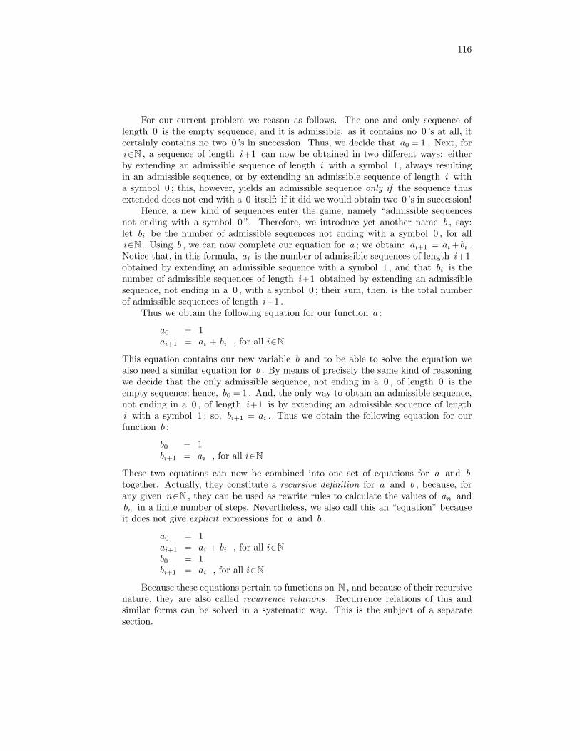
116

For our current problem we reason as follows. The one and only sequence oflength 0 is the empty sequence, and it is admissible: as it contains no 0 ’s at all, itcertainly contains no two 0 ’s in succession. Thus, we decide that a0 = 1 . Next, fori∈N , a sequence of length i+1 can now be obtained in two different ways: eitherby extending an admissible sequence of length i with a symbol 1 , always resultingin an admissible sequence, or by extending an admissible sequence of length i witha symbol 0 ; this, however, yields an admissible sequence only if the sequence thusextended does not end with a 0 itself: if it did we would obtain two 0 ’s in succession!

Hence, a new kind of sequences enter the game, namely “admissible sequencesnot ending with a symbol 0 ”. Therefore, we introduce yet another name b , say:let bi be the number of admissible sequences not ending with a symbol 0 , for alli∈N . Using b , we can now complete our equation for a ; we obtain: ai+1 = ai + bi .Notice that, in this formula, ai is the number of admissible sequences of length i+1obtained by extending an admissible sequence with a symbol 1 , and that bi is thenumber of admissible sequences of length i+1 obtained by extending an admissiblesequence, not ending in a 0 , with a symbol 0 ; their sum, then, is the total numberof admissible sequences of length i+1 .

Thus we obtain the following equation for our function a :

a0 = 1ai+1 = ai + bi , for all i∈N

This equation contains our new variable b and to be able to solve the equation wealso need a similar equation for b . By means of precisely the same kind of reasoningwe decide that the only admissible sequence, not ending in a 0 , of length 0 is theempty sequence; hence, b0 = 1 . And, the only way to obtain an admissible sequence,not ending in a 0 , of length i+1 is by extending an admissible sequence of lengthi with a symbol 1 ; so, bi+1 = ai . Thus we obtain the following equation for ourfunction b :

b0 = 1bi+1 = ai , for all i∈N

These two equations can now be combined into one set of equations for a and btogether. Actually, they constitute a recursive definition for a and b , because, forany given n∈N , they can be used as rewrite rules to calculate the values of an andbn in a finite number of steps. Nevertheless, we also call this an “equation” becauseit does not give explicit expressions for a and b .

a0 = 1ai+1 = ai + bi , for all i∈Nb0 = 1bi+1 = ai , for all i∈N

Because these equations pertain to functions on N , and because of their recursivenature, they are also called recurrence relations. Recurrence relations of this andsimilar forms can be solved in a systematic way. This is the subject of a separatesection.

117

question 3:

What is the number of subsets of a given finite set? Well, every element may or maynot be an element of a subset: for every element of the given set we have a choice outof 2 possibilities, independently of (the choices for) the other elements. Therefore, ifthe given set has n elements, we have n independent choices out of 2 possibilities;hence, the number of subsets of a set with n elements equals 2n .

Actually, this is the very same problem as the one in question 1. The elements ofany finite set can be ordered into a finite sequence, and now every subset of it can berepresented as a sequence of length n consisting of symbols 0 and 1 : a 1 in a givenposition encodes that the corresponding – according to the order chosen – element ofthe given set is an element of the subset, and a 0 in a given position encodes that thecorresponding element of the given set is not an element of the subset. Thus, thereis a one-to-one correspondence – that is: a bijection – between the set of all subsetsof a given set of size n and the set of all sequences of length n consisting of symbols0 and 1 . Thus, question 3 and question 1 are essentially the same, and so are theiranswers.

question 4:

What is the number of elements of the Cartesian product of two given finite sets? LetV and W be finite sets with m and n elements, respectively. The Cartesian productV×W is the set of all pairs (v, w) with v∈V and w∈W . Because v can be chosenout of m elements, and because, independently, w can be chosen out of n elements,the number of possible pairs equals m×n . So, we have: # (V×W ) = #V ∗ #W .

Similarly, the number of elements of the Cartesian product of three finite sets isthe product of the three sizes of these sets: # (U×V×W ) = #U ∗ #V ∗ #W , andso on. The following two questions contain applications of this.

question 5:

What is the number of possible Hungarian license plates for cars? (A Hungarianlicense plate contains three letters followed by three digits.) Each letter is chosen fromthe alphabet of 26 letters, and each digit is one out of 10 decimal digits. Actually,with A for the alphabet and with D for the set of decimal digits, a Hungarian licenseplate number is an element of the Cartesian product A×A×A×D×D×D ; hence, thenumber of possible combinations equals #A ∗ #A ∗ #A ∗ #D ∗ #D ∗ #D , that is:263 ∗ 103 .

question 6:

What is the number of relations on a given finite set? A relation on a set V is asubset of the Cartesian product V×V , so the number of relations on V equals thenumber of subsets of V×V . If V has n elements then V×V has n2 elements, sothe number of relations equals 2n2

.

118

question 7:

What is the number of sequences of length n and containing each of the numbers0 , 1 , · · · , n−1 (exactly) once? Notice that the requirement “containing each of thenumbers 0 , 1 , · · · , n−1 (exactly) once” is rather over specific: that it is about thenumbers 0 , 1 , · · · , n−1 is not very relevant, all that matters is that the sequence con-tains n given different objects. The element in the first position can be chosen outof n possible objects, and this leaves only n−1 objects for the remainder of the se-quence. Hence, the second element can be chosen out of these n−1 objects, and this,in turn, leaves n−2 objects for the (next) remainder of the sequence; and so on, untilwe are left with exactly one object to choose from for the last element of the sequence.Hence, the number of possible such sequences equals n ∗ (n−1) ∗ (n−2) ∗ · · · ∗ 2 ∗ 1 ;this quantity is usually denoted as n! – “n factorial” – .

Here, too, a recursive characterization is possible. The number of sequences oflength 1 , and containing one given object exactly once, equals 1 . And, for any n∈N ,a sequence of length n+1 containing each of n+1 different objects exactly once canbe constructed, firstly, by choosing one of these objects, which can be done in n+1ways, and, secondly, by constructing a sequence of length n containing each of theremaining n objects exactly once; finally, the sequence thus obtained is extended withthe single object chosen in the first step. We conclude that the number of sequencesof length n+1 equals n+1 times the number of sequences of length n . Thus wearrive at this, well-known, recursive definition of n! :

1! = 1(n+1)! = (n+1) ∗ n! , for all n∈N+

question 8:

What is the number of sequences of length n and containing different objects chosenfrom a given collection of m different objects, for given n,m : 1≤n≤m ? One way toapproach this problem is to observe that the m given objects can be arranged into asequence in m! ways, as we have seen in the previous question. The first n objectsof such a sequence then constitute a sequence of length n and containing differentobjects chosen from the given collection of m objects. The order of the remainingm−n objects (in the sequence of length m ), however, is completely irrelevant: theseremaining objects can be ordered in (m−n)! ways, so there are actually (m−n)!sequences of length n , that all begin with the same n objects in the same order, andthat only differ in the order of their last m−n elements. So, to count the numberof sequences of length n we have to divide the number of sequences of length m by(m−n)! . Thus we obtain as answer to our question: m!/ (m−n)! .

question 9:

What is the number of ways to select m objects from a given collection of n objects,for given m,n : 1≤m≤n ? One may well wonder if, and if so how, this question differsfrom the previous one. Well, the previous question was about sequences, whereas this

119

question is about sets. The question can be rephrased as: What is the number ofsubsets of size n of a given set of size m , for given n,m : 1≤n≤m ? Well, everysequence of length n of the kind in the previous question represents such a subset,albeit that the order in which the objects occur in the sequence now is irrelevant.That is, every two sequences, of length n , containing the same objects in possiblydifferent orders now represent the same subset. Actually, for every selection of nobjects there are n! sequences containing these objects and all representing the samesubset. Hence, the number of ways to form a subset of size m from a given set ofsize n equals the answer to the previous question divided by n! . Thus we obtain:m!/ ( (m−n)! ∗n!) . This quantity is called a binomial coefficient and it is usually

denoted as(mn

), which is defined by:

(mn

)=

m!(m−n)! ∗ n!

.

Binomial coefficients happen to have interesting properties which we will study later.

question 10:

What is the number of numbers, in the decimal system, the digits of which are alldifferent? Obviously, such a number consists of at most 10 digits. It is questionablewhether we allow such a number to start with the digit 0 : on the one hand, “0123”does represent a number in the decimal system, on the other hand, we usually donot write down such leading zeroes because they are meaningless: “0123” representsthe same number as “123”. So, let us decide to exclude meaningless leading zeroes.Then, the only number starting with the digit 0 is “0”.

In this case, the problem is most easily solved by distinguishing the possiblenumbers according to their length. We have already observed that the length ofour numbers is at most 10 . For numbers consisting of a single digit we have 10possibilities, as each of the 10 decimal digits is permitted. For numbers of lengthn+1 , 1≤n≤9 , we can choose the first digit in 9 ways, 0 having been excluded asthe first digit. Independently of how this first digit has been chosen we still have 9digits left for the remaining n digits of the number, because now digit 0 is includedagain. So, for these remaining n digits the question becomes: what is the numberof sequences of n digits, chosen from a set of 9 different digits? This question,however, is an instance of problem 8, with m := 9 ; hence, the answer to this questionis 9!/(9−n)! . Thus, we conclude that the number of numbers, in the decimal system,the digits of which are all different, is 10 single-digit numbers, and 9 ∗ 9!/(9−n)!numbers consisting of n+1 digits, for 1≤n≤9 .

question 11:

What is the number of “words” consisting of 5 letters? This depends on what oneconsiders a “word”. If we are asking for the number of 5 -letter words in a specificlanguage the question is a linguistic question, not a mathematical one. So, let us

120

decide that a “word” is just an arbitrary sequence consisting of letters from the 26 -letter alphabet. Then, for every position in the sequence we have an independentchoice out of 26 possibilities, so the number of 5 -letter words equals 265 .

Notice that this question is very similar to questions 1 and 4.

question 12:

What is the number of ways in which 5 pairs can be formed from a group of 10persons? This question does not admit a simple, straightforward answer. Therefore,as in the discussion of question 2, we introduce a variable to represent it: let ai bethe number of ways in which i pairs can be formed from a group of 2 ∗ i persons, forall i∈N+ . The original question, then, amounts to asking for the value of a5 .

For a group of 2 persons, the answer is quite simple: only one pair can be formed,so a1 = 1 . For a group of 2 ∗ (i+1) persons, which is equal to 2 ∗ i+2 , one personcan be matched to 2 ∗ i+1 other persons, and the remaining 2 ∗ i persons can then bearranged into pairs in ai ways. Thus we obtain: ai+1 = (2 ∗ i+1) ∗ ai . Combiningthese results we obtain the following recurrence relations for a :

a0 = 1ai+1 = (2 ∗ i+1) ∗ ai , for all i∈N+

So, informally, we have: ai = (2∗i−1) ∗ (2∗i−3) ∗ · · · ∗ 3 ∗ 1 , and the answer for agroup of 10 persons is 9 ∗ 7 ∗ 5 ∗ 3 ∗ 1 . In some textbooks, the expression for ai isdenoted as (2∗i−1)!! .

question 13:

What is the number of n×n matrices, all elements of which are 0 or 1 ? How manyof these have an odd determinant? The first question has no relation to linear algebra.An n×n matrix has n2 elements, each of which may be 0 or 1 . Hence, the numberof such matrices equals 2n2

. This answer is the same as the answer to question 6,and this is no coincidence. Why?

The problem posed in the second question does belong to linear algebra. Theanswer, which we shall not explain here, is that the number of n×n 0/1 -matriceswith an odd determinant is given by this nice formula:

(Πi : 0≤i<n : 2n−2i ) .

For n= 3 , for example, we thus find 168 matrices with an odd determinant, and344 , namely: 232

−168 , with an even determinant.

question 16:

In a digital signaling system 8 wires are used, each of which may or may not carry avoltage. For the transmission of a, so-called, “code word” via these wires exactly 4wires carry a voltage (and the other 4 wires carry no voltage). How many code wordsare thus possible? Every code words corresponds to a particular selection of 4 wires

121

from the 8 available wires, so the number of possible code words equals the numberof ways to select 4 objects out of a collection of 8 . This is exactly question 9, withn := 4 and m := 8 . Hence, the answer is 8!/(4! ∗ 4!) , which equals 70 .

6.2 Recurrence Relations

6.2.1 An example

In the introduction we have discussed this question: What is the number of sequencesof length n and constructed from the symbols 0 and 1 only, but containing no two0 ’s in succession, for any given natural n ? For the sake of brevity we have calledsuch sequences “admissible”.

To solve this problem we have introduced two functions, a and b , on N , withthe following interpretation, for all i∈N :

ai = “the number of admissible sequences of length i , and:

bi = “the number of admissible sequences of length i,not ending with a 0 ” .

The answer to the above question then is an , and we already have formulated thefollowing set of equations for a and b , also called recurrence relations:

(0) a0 = 1(1) ai+1 = ai + bi , for all i∈N(2) b0 = 1(3) bi+1 = ai , for all i∈N

These recurrence relations form equations for two unknowns, namely a and b .We can, however, use (2) and (3) to eliminate b from equation (1) : after all, we canview (2) and (3) as a definition for b in terms of a . Because of the case distinctionbetween b0 and bi+1 we must apply a similar case distinction to (1) ; that is, wemust split (1) into separate equations for a1 and ai+2 . In the equation for a1 wecan now substitute 1 for b0 (and 1 for a0 ) , and in the equation for ai+2 we cannow substitute ai for bi+1 . Thus we obtain a new set of equations for a in which bdoes not occur anymore:

(4) a0 = 1(5) a1 = 2(6) ai+2 = ai+1 + ai , for all i∈N

Thus, we have obtained a recurrence relation for a in isolation – that is, withoutb – ; the “old” equations (2) and (3) can now be used to define b in terms of a , ifso desired. That is to say, if we are able to derive an explicit – that is, non-recursive –definition for a then (2) and (3) provide an equally explicit definition for b in termsof a . Notice, however, the proviso “if so desired”: we may very well be interested inb too, but our original problem was about a , and we have only introduced b as anadditional, auxiliary variable to be able to formulate equation (1) .

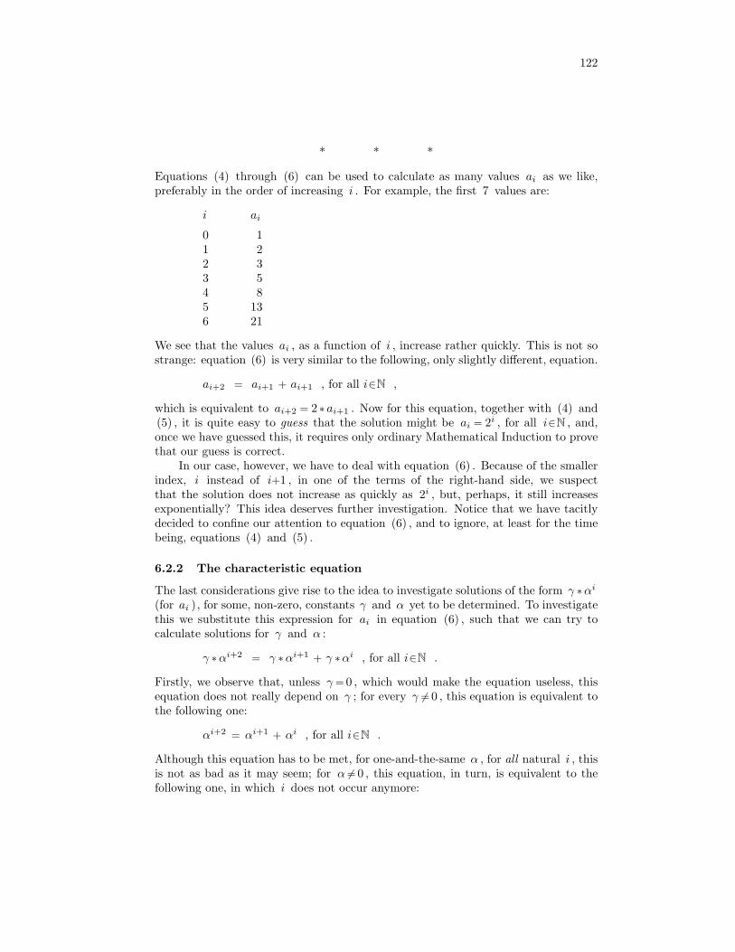
122

* * *

Equations (4) through (6) can be used to calculate as many values ai as we like,preferably in the order of increasing i . For example, the first 7 values are:

i ai

0 11 22 33 54 85 136 21

We see that the values ai , as a function of i , increase rather quickly. This is not sostrange: equation (6) is very similar to the following, only slightly different, equation.

ai+2 = ai+1 + ai+1 , for all i∈N ,

which is equivalent to ai+2 = 2 ∗ ai+1 . Now for this equation, together with (4) and(5) , it is quite easy to guess that the solution might be ai = 2i , for all i∈N , and,once we have guessed this, it requires only ordinary Mathematical Induction to provethat our guess is correct.

In our case, however, we have to deal with equation (6) . Because of the smallerindex, i instead of i+1 , in one of the terms of the right-hand side, we suspectthat the solution does not increase as quickly as 2i , but, perhaps, it still increasesexponentially? This idea deserves further investigation. Notice that we have tacitlydecided to confine our attention to equation (6) , and to ignore, at least for the timebeing, equations (4) and (5) .

6.2.2 The characteristic equation

The last considerations give rise to the idea to investigate solutions of the form γ ∗αi

(for ai ), for some, non-zero, constants γ and α yet to be determined. To investigatethis we substitute this expression for ai in equation (6) , such that we can try tocalculate solutions for γ and α :

γ ∗αi+2 = γ ∗αi+1 + γ ∗αi , for all i∈N .

Firstly, we observe that, unless γ= 0 , which would make the equation useless, thisequation does not really depend on γ ; for every γ 6= 0 , this equation is equivalent tothe following one:

αi+2 = αi+1 + αi , for all i∈N .

Although this equation has to be met, for one-and-the-same α , for all natural i , thisis not as bad as it may seem; for α 6= 0 , this equation, in turn, is equivalent to thefollowing one, in which i does not occur anymore:

123

α2 = α1 + α0 .

Using that α0 = 1 and bringing all terms to one side of the equality we rewrite theequation into this form:

(7) α2 − α1 − 1 = 0 .

This is called the characteristic equation of recurrence relation (6) . What we haveobtained now is the knowledge that if the solution to (6) is to be of the shape γ ∗αi

then α must satisfy (7) .Equation (7) is a quadratic one with two solutions α0 and α1 , say, given by:

(8) α0 = (1+√

5 )/2 and: α1 = (1−√

5 )/2 .

Apparently, we have two possibilities for α here, so ai = αi0 and ai = αi

1 are bothsolutions to our original equation (6) , but there is more. We recall equation (6) :

(6) ai+2 = ai+1 + ai , for all i∈N .

As we will discuss more extensively later, this is a so-called linear and homogeneousrecurrence relation, which has the property that any linear combination of solutionsis a solution as well. In our case, this means that for all possible constants γ0 andγ1 , the definition:

(9) ai = γ0 ∗αi0 + γ1 ∗αi

1 , for all i∈N ,

provides a solution to equation (6) . In fact, it can be proved that all solutions havethis shape, so now we have obtained all solutions to equation (6) .

Recurrence relations (4) through (6) , however, which also constitute a recursivedefinition for a , suggest that the solution should be unique. After all, we are able toconstruct a table containing the values ai , for increasing i , as we did in the previoussection. So, which one out of the infinitely many solutions of the shape given by (9)is the one we are looking for? This means: what should be the values of constants γ0

and γ1 such that we obtain the correct solution? To answer this question we have toconsider equations (4) and (5) again, the ones we have temporarily ignored:

(4) a0 = 1(5) a1 = 2

If we now instantiate (9) , with i := 0 and i := 1 , and using that α0 = 1 and α1 = α ,for any α , we obtain these two special cases:

a0 = γ0 + γ1 and: a1 = γ0 ∗α0 + γ1 ∗α1 .

By substituting these values for a0 and a1 into equations (4) and (5) we obtain thefollowing two new equations, in which γ0 and γ1 are the unknowns now:

γ0 + γ1 = 1γ0 ∗α0 + γ1 ∗α1 = 2

124

With γ0 and γ1 as the unknowns, these are just two linear equations that can besolved by standard algebraic means. In this case we obtain:

γ0 = (2−α1)/(α0−α1) and: γ1 = (α0−2)/(α0−α1) ,

where α0 and α1 are given, above, by definition (8) . Thus we obtain, for all i∈N :

(10) ai = ( (3+√

5 )/2√

5 ) ∗ ( (1+√

5 )/2)i + ( (√

5−3)/2√

5 ) ∗ ( (1−√

5 )/2)i .

The sequence f0, f1, f2, . . . defined by

f0 = 0, f1 = 1, fn+2 = fn+1 + fn for n ≥ 0

is usually called the Fibonacci sequence, named after Fibonacci, also called Leonardofrom Pisa, who lived from around 1170 to around 1250. This sequence has manyapplications in computer science. It is closely related to the sequence ai inverstigatedabove, in fact ai = fi+2 for all i ≥ 0. In the same way as above one derives

fi =(1+√

5 /2)i − (1−√

5 /2)i

√5

for all i ≥ 0. Note that (1+√

5 )/2 ≈ 1.618 and (1−√

5 )/2 ≈ −0.618, so (1−√

5 /2)i

converges very quickly to 0, and up to a constant fi is roughly equal to (1.618)i forlarger i, which grows exponentially.

6.2.3 Linear recurrence relations

The recurrence relation studied in the previous section belongs to a class of recurrencerelations known as linear recurrence relations with constant coefficients. They arecalled linear because function values, like ai+2 , are defined as linear combinationsof other function values, like ai+1 and ai in (6) . Notice that equation (6) can bewritten, slightly more explicitly, as:

ai+2 = 1 ∗ ai+1 + 1 ∗ ai , for all i∈N .

Any formula of the shape c0 ∗x0 + c1 ∗x1 + c2 ∗x2 + · · · is called a linear com-bination of the x s, with the c s being the coefficients. In the case of recurrencerelations, we speak of constant coefficients if they do not depend on i . For example,in our example the coefficients, of ai+1 and ai , are 1 and 1 , respectively, which,indeed, do not depend on i .

The general shape of a linear recurrence relation with constant coefficients is thefollowing one, in which the cj are the coefficients, for all j : 0≤j<k , c0 6= 0, and inwhich k is a constant called the order of the recurrence relation:

(11) ai+k = ck−1 ∗ ai+k−1 + · · · + c1 ∗ ai+1 + c0 ∗ ai , for all i∈N.

125

So, in a k -th order recurrence relation value ai+k is defined recursively in terms ofits k direct predecessors, which are ai+k−1 , · · · , ai+1 , ai , only.

Relation (11) defines ai+k recursively in terms of ai+k−1 , · · · , ai+1 , ai , as alinear combination, for all i∈N , but it does not define the first k elements of functiona ; that is, relation (11) gives no information on the values ak−1 , · · · , a1 , a0 . Thesevalues, therefore, may be, and must be, defined separately. So, a complete k -th orderrecurrence relation consists of relation (11) together with k separate definitions forthe values ai , for all i : 0≤i<k . These definitions also are known as the initialconditions of the recurrence relation.

* * *

Relation (11) is homogeneous, which means that if αi is a solution for ai , then so isγ ∗αi , for any constant γ . Relation (11) is linear , which means that if αi and βi

both are solutions for ai , then so is αi +βi . Combining these two observations weconclude that any linear combination of solutions to (11) is a solution as well. Notethat this conclusion only pertains to equation (11) in isolation, so without regard forthe initial conditions. If the initial conditions are taken into account the recurrencerelation has only one, unique, solution.

As in the example before, we now investigate to what extent equation (11)admits solutions of the shape αi for ai . Notice that, because of the homogeneity, wedo not need to incorporate a constant coefficient: as was the case with the solution tothe example – Section 6.2.2 – , this coefficient will drop out of the equation anyhow.Substitution of αi for ai in (11) transforms it into the following equation for α :

αi+k = ck−1 ∗αi+k−1 + · · · + c1 ∗αi+1 + c0 ∗αi , for all i∈N .

As we are looking for solutions with α 6= 0 , this equation can be further simplifiedinto this, equivalent, form:

(12) αk − ck−1 ∗αk−1 · · · − c1 ∗α − c0 ∗ 1 = 0 .

Now αi is a solution for ai in equation (11) if and only if α is a solution toequation (12) , which, as before, is called the characteristic equation of the recurrencerelation. Notice that this is an algebraic equation of the same order as the order ofthe recurrence relation.

* * *

The simplest case arises when the k -th order characteristic equation has k differentreal roots, αj , say, for j : 0≤j<k . Then, any linear combination of the powers ofthese roots, that is, for all possible coefficients γj , with 0≤j<k , function a definedby:

(13) ai = (Σj : 0≤j<k : γj ∗αij ) , for all i∈N ,

126

is a solution to (11) . Moreover, not only does this yield just a solution to (11) , itcan even be proved that all solutions are thus characterized.

As stated before, when the k initial conditions, that is, the defining relationsfor ai , for 0≤i<k , are taken into account, the solution to the recurrence relation isunique. This means that if the values for ai , for 0≤i<k , have been given, and oncethe αj , for 0≤j<k haven been solved from (11) , definition (13) , for all i : 0≤i<k ,is not a definition anymore but a restriction on the possible values for γj . That is,the set of relations:

(Σj : 0≤j<k : γj ∗αij ) = ai , for all i : 0≤i<k ,

now constitutes a system of k linear equations with unknowns γj , with 0≤j<k , fromwhich these can be solved by means of standard linear-equation solving techniques.

* * *

A somewhat more complicated situation arises if the characteristic equation has mul-tiple roots. A simple example of this phenomenon is the equation:

α2 − 2.8 ∗α + 1.96 = 0 ,

which can be rewritten as:

(α−1.4)2 = 0 .

This means that both roots α0 and α1 are equal to 1.4 .In a general k -th order algebraic equation a root may have a, so-called, multi-

plicity upto k . It can now be proved that, if a certain root αp , say, has, multiplicityq , say, then αi

p , i ∗αip , i2 ∗αi

p , · · · , iq−1 ∗αip are q independent solutions for ai

in equation (11) . These q different solutions account for the multiplicity, also q , ofroot αp . Thus, in total we still obtain k different basis solutions from which linearcombinations can be formed to obtain, again, all solutions of the recurrence relation.

As a simple example, the characteristic equation:

α2 − 2.8 ∗α + 1.96 = 0 ,

has a single root, 1.4 , with multiplicity 2 . Hence, all solutions to the (homoge-neous) recurrence relation of which this is the characteristic equation are of the formγ0 ∗ 1.4i + γ1 ∗ i ∗ 1.4i .

* * *

The situation becomes even more complicated if the characteristic equation has lessthan k , possibly multiple, roots in R : then the equation still has k roots, but some(or all) of them are complex numbers. A very simple example is the equation:

α2 − α + 1 = 0 .

127

As the determinant, namely 1−4 , of this equation is negative, this equation has noroots in R at all, but it has two complex numbers as its roots: (1+

√−3 )/2 and

(1−√−3 )/2 , which are usually written as – with i=

√−1 – : (1+ i ∗

√3 )/2 and

(1− i ∗√

3 )/2 .These complex roots can be used, in the same way as described earlier, to obtain

all solutions to the recurrence relation. Although, definitely, there is quite somemathematical beauty in this, such solutions are not very useful from a practical pointof view. In Subsection ?? we present a more computational way to cope with suchsituations.

6.2.4 Summary

Summarizing, for solving a recurrence relation of the shape

a0 = n0, a1 = n1, ai+2 = c1ai+1 + c0ai for all i ∈ N

for given numbers n0, n1, c0, c1, we have the following approach:

• First ignore the requirements a0 = n0, a1 = n1 and try to find a solution ofai+2 = c1ai+1 + c0ai of the shape ai = αi for all i. This yields the characteristicequation α2 = c1α+ c0.

• Find the two solutions α0 and α1 of this equation, now for every two numbersA,B, the expression ai = Aαi

0 +Bαi1 is a solution of the equation. The numbers

α0 and α1 may be real or complex numbers. In case α0 = α1, then the expressionai = Aαi

0 +Biαi0 is a solution of the equation.

• Finally, find values for A,B such that a0 = n0, a1 = n1 hold.

We observe that if n0, n1, c0, c1 ∈ N then we will obtain ai ∈ N for all i. Inparticular, this holds for counting problems as in our introduction, which are onlyabout natural numbers. For integer n0, n1, c0, c1 the result will always be integer. Inthe mean time we have obtained a solution of the form (10) , in which both α0 , α1 ,and the coefficients A,B are defined in terms of true – non-integer, even irrational –real numbers like

√5 , or even complex numbers. Apparently, however complicated

the resulting formula is, its value is a natural number nevertheless. Isn’t that strange?We conclude that even for problems that are purely about natural or integer

numbers, it turns out to be fruitful to make an excursion into R or C to be able tofind a closed expression for the solution of the problem.

6.3 Binomial Coefficients

6.3.1 Factorials

We already have seen that the product n ∗ (n−1) ∗ (n−2) ∗ · · · ∗ 2 ∗ 1 is denoted asn! – “n factorial” – , for any n∈N+ . Even for n= 0 this product is meaningful: thenit is the empty product, consisting of 0 factors, for which the best possible definitionis the identity element of multiplication, that is: 1 . A recursive definition for n! is:

128

0 ! = 1(n+1) ! = (n+1) ∗ n! , for all n∈N

Factorials occur in solutions to many counting problems. In Section 6.1 we alreadyhave argued that the number of ways to arrange n given, different objects into asequence of length n equals n! . Here we repeat the argument, in a slightly moreprecise way. We do this recursively; for this purpose, we introduce a function a onN with the idea that:

ai = “the number of sequences of length i, containing i different objects” ,for all i∈N .

The number of ways to arrange 0 different objects into a sequence of length 0 equals1 , because the only sequence of length 0 is the empty sequence, and it contains 0objects. So, we conclude: a0 = 1 . Next, to arrange i+1 different objects into asequence of length i+1 we can, firstly, select one object that will be the first elementof the sequence, and, secondly, arrange the remaining i objects into a sequence oflength i . The first object can be selected in i+1 different ways and, independently,the remaining i objects can be arranged in ai ways into a sequence of length i . So,we obtain: ai+1 = (i+1) ∗ ai . Thus, we obtain as recurrence relation for a :

a0 = 1ai+1 = (i+1) ∗ ai , for all i∈N

The solution to this recurrence is ai = i! , for all i∈N .Notice that, while we are speaking here of “different objects”, their actual nature

is irrelevant: all that matters is that they are different. Actually, we even have usedthis tacitly in the above argument: after we have selected one object from a collectionof i+1 different objects, the remaining collection, after removal of the object selected,is a collection of i different objects, independently of which object was selected to beremoved.

* * *

A slightly more complicated problem we also have discussed in Section 6.1 was: whatis the number of ways to select and arrange n different objects from a given collectionof m different objects into a sequence of length n , for given n,m : 0≤n≤m ?

One way to approach this problem is to observe that, as we now know, the mgiven objects can be arranged into a sequence in m! ways. The first n objects of sucha sequence then constitute a sequence of length n that contains n different objectschosen from the given collection of m objects. The order of the last m−n objects(in the sequence of length m ) , however, is completely irrelevant: these remainingobjects can be ordered in (m−n)! ways without affecting the first n objects in thesequence, so there are actually (m−n)! sequences of length n , that all begin withthe same n objects in the same order, and that only differ in the order of theirlast m−n elements. So, to count the number of sequences of length n we have todivide the number of sequences of length m by (m−n)! . Thus we obtain as solution:m!/ (m−n)! .

129

6.3.2 Binomial coefficients

The number of ways to select an (unordered) collection – instead of an (ordered)sequence – of n different objects from a given collection of m different objects, forn,m : 0≤n≤m , can be determined by the following argument. The number of waysto arrange n different objects into a sequence is, as we know, n! . If we are onlyinterested in a collection of such objects, their order is irrelevant, and this meansthat all n! such arrangements are equivalent. So, to obtain the number of possiblecollections we must, again, divide the answer to the previous problem by n! . Thus,we obtain as solution:

m!n! ∗ (m−n)!

.

It so happens that this is an important quantity that has many interesting properties.These quantities are called binomial coefficients, and we introduce a notation for it,which is pronounced as “m over n”:(

mn

)=

m!n! ∗ (m−n)!

, for all n,m : 0≤n≤m .

* * *

For example, we consider all sequences of length m consisting of (binary) digits –“bits”, for short – 0 or 1 . As every bit in such a sequence is either 0 or 1 – so,one out of two possibilities – , independently of the other bits in the sequence, thetotal number of bit sequences of length m equals 2m . If we number the positionsin such a sequence from and including 0 and upto and excluding m , a one-to-onecorrespondence – that is, a bijection – exists between the collection of all subsets ofthe interval [ 0 . .m ) and the collection of all bit sequences of length m : numberi is in a given subset if and only if the corresponding sequence contains a bit 1 atposition i , for all i∈ [ 0 . .m ) .

The collection of bit sequences of length m can be partitioned into m+1 disjointclasses, according to the number of bits 1 in the sequence. That is, we consider thebit sequences, of length m , containing exactly n bits 1 , for n,m : 0≤n≤m . In thesubset↔bit-sequence correspondence every bit sequence containing exactly n bits 1now corresponds to a subset with exactly n elements.

We already know that the number of subsets containing exactly n elements

chosen from a given collection of m elements equals(mn

). Hence, because of the

one-to-one correspondence, the number of bit sequences of length m and containing

exactly n bits 1 also equals(mn

).

Because the bit sequences of length m and containing exactly n bits 1 , for alln with 0≤n≤m , together are all bit sequences of length m , we obtain the following,quite interesting result:

(Σn : 0≤n≤m :(mn

)) = 2m , for all m∈N .

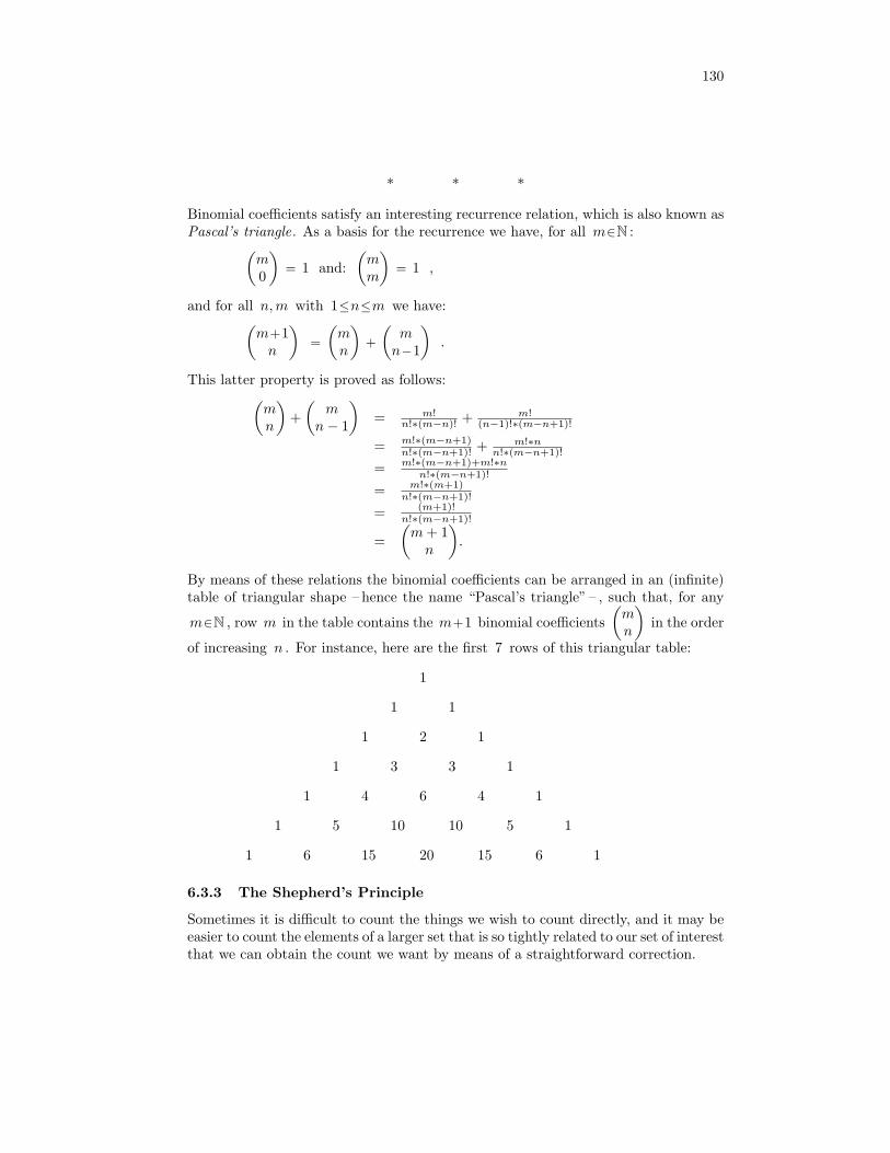
130

* * *

Binomial coefficients satisfy an interesting recurrence relation, which is also known asPascal’s triangle. As a basis for the recurrence we have, for all m∈N :(

m0

)= 1 and:

(mm

)= 1 ,

and for all n,m with 1≤n≤m we have:(m+1n

)=

(mn

)+

(mn−1

).

This latter property is proved as follows:(mn

)+(

mn− 1

)= m!

n!∗(m−n)! + m!(n−1)!∗(m−n+1)!

= m!∗(m−n+1)n!∗(m−n+1)! + m!∗n

n!∗(m−n+1)!

= m!∗(m−n+1)+m!∗nn!∗(m−n+1)!

= m!∗(m+1)n!∗(m−n+1)!

= (m+1)!n!∗(m−n+1)!

=(m+ 1n

).

By means of these relations the binomial coefficients can be arranged in an (infinite)table of triangular shape – hence the name “Pascal’s triangle” – , such that, for any

m∈N , row m in the table contains the m+1 binomial coefficients(mn

)in the order

of increasing n . For instance, here are the first 7 rows of this triangular table:

1

1 1

1 2 1

1 3 3 1

1 4 6 4 1

1 5 10 10 5 1

1 6 15 20 15 6 1

6.3.3 The Shepherd’s Principle

Sometimes it is difficult to count the things we wish to count directly, and it may beeasier to count the elements of a larger set that is so tightly related to our set of interestthat we can obtain the count we want by means of a straightforward correction.

131

This is known as the Shepherd’s Principle, because of the following metaphor. Tocount the number of sheep in a flock of sheep may be difficult: when the sheep stickclosely together one observes a single, cluttered mass of wool in which no individualsheep can be distinguished easily. But, knowing – and assuming! – that every sheephas 4 legs, we can count the legs in the flock and conclude that the number of sheepequals this number of legs divided by 4 .

As a matter of fact, we have already applied this technique, in Subsection 6.3.1:to count the number of sequences of length n and containing n different objectsfrom a given collection of m different objects – the sheep – , we have actually countedthe number of sequences of length m – the legs – and divided this by the number ofways the irrelevant m−n remaining objects can be ordered – the number of legs persheep – .

* * *

To demonstrate the Shepherd’s Principle we discuss a few simple examples. Firstly,the number of anagrams of the word “FLIPJE” just equals the numbers of ways inwhich the 6 different letters can be arranged into a sequence of length 6 . This issimple because the 6 letters are different, and the answer just is 6! .

Secondly, what is the number of anagrams of the word “SHEPHERD”? As thisword contains 8 letters there would be, if all letters would be different, 8! ways toarrange them into an anagram. But the letters are not different: the word contains 2letters “H” and 2 letters “E”; here we assume, of course, that the 2 letters “H” areindistinguishable and also that the 2 letters “E” are indistinguishable. Well, we makethem different temporarily , by tagging them, for example, by means of subscripts:“SH0E0PH1E1RD”. Now all letters are different, and the number of anagrams of thisword – the legs – equals 8! . The number of legs per sheep now is the number of waysin which the tagged letters can be arranged: E0 and E1 can be arranged in 2! waysand, similarly, H0 and H1 can be arranged in 2! ways. So, the number of legs persheep equals 2! ∗ 2! , and, hence, the number of anagrams of “SHEPHERD” – thenumber of sheep – equals 8!/ (2! ∗ 2!) .

Thirdly, what is the number of anagrams of the word “HAHAHAH”? Well, this7 -letter word contains 4 letters “H” and 3 letters “A”; so, on account of the Shep-

herd’s Principle, the answer is 7!/ (4! ∗ 3!) , which equals(

74

). Is this a surprise?

No, because the word is formed from only 2 two different letters, “H” and “A”; so,the number of anagrams of “HAHAHAH” is equal to the number of 7 -letter words,formed from letters “H” and “A” only and containing exactly 4 letters “H”.

As the exact nature of the objects is irrelevant – it really does not matter whetherwe use “H” and “A” or “1” and “0” – , this last question is the same as the questionfor the number of 7 -bit sequences containing exactly 4 bits 1 . Hence, the answersare the same as well.

6.3.4 Newton’s binomial formula

In subsection 6.3.2 we have derived the following relation for binomial coefficients:

132

(Σn : 0≤n≤m :(mn

)) = 2m , for all m∈N .

Actually, this is an instance of the following, more general relation, for all – integer,rational, real, . . . – numbers x, y :

(14) (x+y)m = (Σn : 0≤n≤m :(mn

)∗xn ∗ ym−n ) , for all m∈N .

This is known as Newton’s binomial formula, although it appears to be much olderthan Newton. Newton, however, has generalized the formula by not restricting m tothe naturals but by allowing it even to be a complex number.

We will not elaborate this here; instead we confine ourselves to the observationthat there is a connection between the recurrence relation for binomial coefficients wehave seen earlier:(

m+1n

)=

(mn

)+

(mn−1

),

and relation (14) , by means of the recurrence relation for exponentiation when appliedto (x+y) :

(x+y)m+1 = (x+y) ∗ (x+y)m .

6.4 A few examples

We conclude this chapter with a few more examples, some of which we have alreadysolved, albeit in a slightly different form.

example 1:

A vase contains m balls which have been numbered 0 , 1 , · · · ,m−1 . From this vasewe draw, at random, n balls, for some n : 0≤n≤m . What is the number of possibleresults if the order in which the balls are drawn is relevant?

Notice that, although the balls themselves may not be distinguishable by theirshapes, the fact that they have been numbered makes them distinguishable. So, whatmatters here is that we have a collection of m different objects. The problem athand now is the same as a question we have already answered earlier: What is thenumber of sequences of length n and containing different objects chosen from a givencollection of m different objects, for given n,m : 1≤n≤m ? As we have seen, theanswer to this question is: m!/ (m−n)! .

example 2:

A vase contains m balls which have been numbered 0 , 1 , · · · ,m−1 . From this vasewe draw, at random, n balls, for some n : 0≤n≤m . What is the number of possibleresults if the order in which the balls are drawn is not relevant? We recall that thisquestion is equivalent to the question: What is the number of subsets of size n of a

given finite set of size m ? As we have seen, the answer is(mn

).

133

We also have seen that an alternative way to answer this question is to apply theShepherd’s Principle: the n balls drawn from the vase can be ordered in n! ways; asthis order is irrelevant we have to divide the answer to the previous question by this

very n! ; as a result, we obtain the same answer, of course:(mn

).

example 3:

A vase contains m balls which have been numbered 0 , 1 , · · · ,m−1 , for some positivenatural m . From this vase we draw, at random, n balls, for some n∈N , but nowevery ball drawn is placed back into the vase immediately, that is, before any nextballs are drawn. What is the number of possible results if the order in which the ballsare drawn is relevant? (Notice that in this example we do not need the restrictionn≤m .) The result of this game simply is a sequence, of length n , of numbers in therange [ 0 . .m ) , and the numbers in this sequence are mutually independent. Hence,the answer is: mn .

example 4:

A vase contains m balls which have been numbered 0 , 1 , · · · ,m−1 , for some positivenatural m . From this vase we draw, at random, n balls, for some n∈N , but nowevery ball drawn is placed back into the vase immediately, that is, before any nextballs are drawn. What is the number of possible results if the order in which the ballsare drawn is not relevant? This example is new, and more difficult that the previousones.

An effective technique to solve this and similar problems is to choose the “right”representation of the possible results of the experiment, namely in such a way thatthese results can be counted. In the current example, we might write the down thenumbers of the balls drawn, giving rise to sequences, of length n , and containingnumbers in the range [ 0 . .m ) . In this case, however, this representation is notunique, because the order of these numbers is irrelevant. For instance, the sequence“3011004” is a possible result, but so are the sequence “4011030” and “0001134”;because the order of the numbers in the sequences is irrelevant and because thesethree sequences contain the same numbers, albeit in different orders, these sequencesactually represent only one result, which should be counted only once. So, we needa unique representation, because only then the number of possible results is equal tothe number of possible representatives of these results.

We obtain a unique representation by writing down the numbers of the ballsdrawn in ascending order : then every result corresponds in a unique way to an as-cending sequence, of length n , and containing numbers in the range [ 0 . .m ) . Forinstance, from the three example sequences “3011004” , “4011030” , and “0001134”,the last one is ascending: it uniquely represents the, one-and-only, common resultcorresponding to these sequences.

So, the answer to our original question equals the number of ascending sequences,of length n , and containing numbers in the range [ 0 . .m ) . To be able to count these

134

smoothly, yet another representation happens to be convenient, based on the followingobservation. The sequence “0001134”, for instance, consists of 3 numbers 0 , followedby 2 numbers 1 , followed by 0 numbers 2 , followed by 1 numbers 3 , followed by1 numbers 4 , followed by 0 numbers 5 , where we have assumed m= 6 and n= 7 .So, by counting, for every number in the range [ 0 . .m ) , how often it occurs inthe ascending sequence we can also represent the result of the experiment. For thesequence “0001134”, for instance, the corresponding sequence of counts is “320110”:it contains m numbers, namely one count for every number in the range [ 0 . .m ) ;each count itself is a number in the range [ 0 , m ] and the sum of all counts equalsn , which was the length of the ascending sequence.

The restriction that the sum of the counts equals n is a bit awkward but canbe made more manageable by means of the following coding trick : we represent eachcount by a sequence of as many zeroes as the count – in the unary representation,so to speak – and we separate these sequences of zeroes by means of a digit 1 . Forinstance, again with m= 6 , the counts of the original ascending sequence “0001134”are 3 , 2 , 0 , 1 , 1 , and 0 , which in the zeroes-encoding become “000”, “00”, “ ”, “0”,“0”, and “ ”. Concatenated and separated by digits 1 we obtain: “000100110101”.This is a bit sequence containing exactly n digits 0 , because now the sum of thecounts simply equals the total number of zeroes, and containing exactly m−1 digits1 , because we have m counts separated by m−1 digits 1 . Consequently, the lengthof this bit sequence is m−1+n .

Generally, every ascending sequence of length n and containing numbers in therange [ 0 . .m ) can be represented uniquely by a bit sequence of length m−1+ncontaining exactly n digits 0 and m−1 digits 1 . So, also the results of our ballsdrawing experiment are uniquely represented by these bit sequences. Therefore, thenumber of all possible results equals the number of these bit sequences, which is:(m−1+n

n

).

6.4.1 Summary

Summarizing, for counting the number of possibilities to draw k copies from a set ofn objects, there are four possible results, depending on the context:

• If every copy is drawn from the full set, so the drawn copies are put back, anddrawings in a different order are considered to be different, then the number ofpossibilities is

nk.

• If every copy is drawn from the remaining set, and no copies are put back, anddrawings in a different order are considered to be different, then the number ofpossibilities is

n(n− 1)(n− 2) · · · (n− k + 1) = n!/(n− k)! = k!(nk

).

135

• If every copy is drawn from the remaining set, and no copies are put back, anddrawings in a different order are considered to be the same, then the number ofpossibilities is(

nk

).

• If every copy is drawn from the full set, so the drawn copies are put back, anddrawings in a different order are considered to be the same, then the number ofpossibilities is(

n− 1 + kk

).

6.5 Exercises

1. Let V be a finite set with n elements.

(a) What is the number of functions in V → 0 , 1 ?

(b) What is the number of functions in V → 0 , 1 , 2 ?

(c) What is the number of functions in V →W , with #W =m ?

2. (a) What is the number of “words” consisting of 5 different letters?

(b) What is the number of injective functions in0 , 1 , 2 , 3 , 4→ a , b , c , · · · , z ?

(c) What is the number of injective functions in V →W , with #V =n and#W =m ?

3. Let wi be the number of sequences, of length i , consisting of letters froma , b , c , in which each two successive letters are different, for all i∈N .

(a) Formulate a recurrence relation for w .

(b) Derive an explicit definition for w .

4. Let vi be the number of sequences, of length i , consisting of letters froma , b , c , in which no two letters a occur in direct succession, for all i∈N . Itis given that vi+2 = 2 ∗ vi+1 +2 ∗ vi , for all i∈N .

(a) Determine v0 and v1 .

(b) Values c0 , c1 ,α0 , and α1 exist such that vi = c0 ∗αi0 +c1 ∗αi

1 , for alli∈N . Determine c0 , c1 ,α0 , and α1 .

5. (a) What is the number of 2 -letter combinations in which the 2 letters occurin alphabetical order? For example: “kx” is such a combination, whereas“xk” is not.

136

(b) What is the number of 3 -letter combinations in which the 3 letters occurin alphabetical order?

(c) What is the number of n -letter combinations in which the n letters occurin alphabetical order, for every natural n : n≤26 ?

6. We consider (finite) sequences g , of length n , consisting of natural numbers,with the additional property that gi≤ i , for all i : 0≤i<n . (Here gi denotesthe element at position i in the sequence, where positions are numbered from0 , as usual.)

(a) What is the number of this type of sequences, as a function of n∈N+ ?

(b) Define a bijection between the set of these sequences and the set of allpermutations of [ 0 . . n ) .

7. This exercise is about strings of beads. The answers to the following questionsdepend on which strings of beads one considers “the same”: therefore, give thissome thought to start with.

(a) What is the number of ways to thread n different beads onto a string?

(b) We have 2 ∗n beads in n different colors; per color we have exactly 2beads, which are indistinguishable. What is the number of ways to threadthese beads onto a string?

(c) The same question, but now for 3 ∗n beads, with 3 indistinguishablebeads per color.

(d) What is the number of ways to thread m red and n blue beads onto astring, if, again, beads of the same color are indistinguishable?

8. The sequence of, so-called, Fibonacci numbers is the function F defined recur-sively by: F0 = 0 , F1 = 1 , and Fi+2 = Fi+1 +Fi , for i∈N . The sequence Sof, so-called, partial sums of F is defined by: Sn = (Σi : 0≤i<n : Fi) , for alln∈N . Prove that Sn = Fn+1− 1 , for all n∈N .

9. What is the number of anagrams of the word “STRUCTURES”?

10. Prove that (Σj : 0≤j<i : 2j ) = 2i−1 , for all i∈N .

11. A given function a on N satisfies: a0 = 0 and ai+1 = ai + i , for all i∈N . Derivean explicit definition for a .

12. A given function a on N satisfies: a0 = 0 and ai+1 = 2 ∗ ai + 2i , for all i∈N .Derive an explicit definition for a .

13. A given function a on N satisfies: a0 = 0 and ai+1 = 2 ∗ ai + 2i+1 , for all i∈N .Derive an explicit definition for a .

14. A given function a on N+ satisfies: a1 = 1 and ai+1 = (1+1/i) ∗ ai , for alli∈N+ . Derive an explicit definition for a .

137

15. At the beginning of some year John deposits 1000 Euro in a savings account,on which he receives 8% interest at the end of every year. At the beginning ofeach next year he withdraws 100 Euro. How many years can John maintain thisbehavior, that is, after how many years the balance of his account is insufficientto withdraw yet another 100 Euro?

16. Solve the following recurrence relations for a function a ; in each of the caseswe have a0 = 0 and a1 = 1 , and for all i∈N :

(a) ai+2 = 6 ∗ ai+1−8 ∗ ai ;

(b) ai+2 = 6 ∗ ai+1−9 ∗ ai ;

(c) ai+2 = 6 ∗ ai+1−10 ∗ ai .

17. Solve the recurrence relation ai+2 = 6 ∗ ai+1 +9 ∗ ai , for all i∈N , with a0 = 6and a1 = 9 .

18. The, so-called, Lucas sequence is the function L defined recursively by: L0 = 2 ,L1 = 1 , and Li+2 = Li+1 +Li , for all i∈N . Determine the first 8 elements ofthis sequence, and derive an explicit definition for L .

19. Let V be a finite set with m elements. Let n satisfy: 0≤n≤m . Whatis the number of functions in V → 0 , 1 , with the additional property that#v∈V | f(v) = 1 = n ?

20. A chess club with 20 members must elect a board consisting of a chairman, asecretary, and a treasurer.

(a) What is the number of ways to form a board (from members of the club)if the three positions must be occupied by different persons?

(b) What is the number of ways if it is permitted that a person occupies severalpositions?

(c) What is the number of ways if the rule is that every person occupies atmost 2 positions?

21. What is the number of sequences, of length 27 , consisting of exactly 9 symbols0 , 9 symbols 1 , and 9 symbols 2 ?

22. In a two-dimensional plane, a robot walks from grid point (0 , 0) to grid point(12 , 5) , by successively taking a unit step, either in the positive x -directionor in the positive y -direction; it never takes a step backwards. What is thenumber of possibles routes the robot can walk?

23. What is the number of 8 -digit decimal numbers in which the digits occur indescending order only? For example, “77763331” is such a number, whereas“98764511” is not.

138

7 Number Theory

7.1 Introduction

The basic arithmetic operations we have learned in primary school are addition, sub-traction, multiplication, and division on natural numbers. These operations are mean-ingful, not only for numbers, but also for more general objects, like functions and, inparticular, polynomials. Some properties of the arithmetic operations remain valid inthese more general structures, whereas other properties lose their validity.

In this chapter we study some of the properties of integer numbers, which arethe numbers · · · ,−2 ,−1 , 0 , 1 , 2 , 3 , · · · . The set of these numbers is called Z ; ithas the set N of the natural numbers 0 , 1 , 2 , 3 , · · · as a subset. So, N includes0 . In the earlier days of mathematics 0 was not considered a natural number, butif we “define” the natural numbers as the numbers used for counting then 0 is avery natural number: at the moment I write this, for instance, I have 0 coins in mypocket. (As a child I have learned that “zero is nothing”, but this is not true, ofcourse: although I have 0 coins in my pocket, it is not empty: it contains 0 coinsbut 1 handkerchief and 1 keyring holding 5 keys.) Also, at any given moment mywallet may contain 3 Euros and 0 U.S. dollars. Moreover, 0 has the, very important,algebraic property that it is the identity element of addition: x+0 = x , for all x∈N(and also for x in Z ,Q ,R , of course). In addition, the natural numbers have theproperty that every natural number is equal to the number of its predecessors, wherethe predecessors of x are all natural numbers less than x : for every x∈N , we havethat x is equal to the number of elements of the set y∈N | y<x , and this is alsotrue if x= 0 .

The set of positive naturals is denoted by N+ ; it equals N but without 0 , so wehave N+ = N\0 . When we discuss the prime numbers we will have need of theset of all natural numbers that are at least 2 , so this is N without 0 and 1 . We willcall such numbers “multiples” and denote its set as N+2 . So, N+2 = N\0 , 1 .

7.2 Divisibility

We start our subject with an exploration of divisibility and its, hopefully well-known,properties.

7.1 Definition. For a, d∈Z we say that “ a is divisible by d ” or, equivalently, that “ ais a multiple of d ” or, equivalently, “ d is a divisor of a ” if and only if:

(∃q : q∈Z : a = q ∗ d ) .2

By this definition, every integer is a divisor of 0 , even 0 itself, although 0/0 is notdefined! If, however, d 6= 0 , then for every a∈Z the value q , if it exists, for whicha = q ∗ d is unique, and we write it as a/d , called the “quotient of” a and d . So,note that a/d is well-defined if and only if both a is divisible by d and d 6= 0 .

139

Other simple properties are that every integer is divisible by 1 and by itself, and, asa consequence, 1 is a divisor of every integer.

The relation “is a divisor of” is often denoted by the (infix) symbol | . Thatis, we write d |a for the proposition “ d is a divisor of a ”. Then, as we have seenearlier, (N+ , | ) is a poset: the relation | is reflexive, anti-symmetric, and transitive.

7.2 Lemma. (∀a, d : a, d∈N+ : d |a ⇒ d≤ a ) .

Proof. If d |a for d, a ∈ N+, then a = q ∗ d for some integer q. Since d, a ∈ N+ this isonly possible for q ≥ 1, so a− d = q ∗ d− d = (q − 1) ∗ d ≥ 0.

A direct consequence of Lemma 7.2 is that the set of all (positive) divisors ofa positive natural number is finite: the set of divisors of a∈N+ is a subset of the(finite) interval [ 1 , a ] . Because 1 |a the set of divisors of a is non-empty, for everya∈N+ .Another important property of divisibility (by d ) is that it is invariant under additionof multiples (of d ) . We call this a translation property .

7.3 Lemma. (∀a, d, x : a, d∈N+ ∧ x∈Z : d |a ⇔ d | (a+x ∗ d) ) .

Proof. If d |a then a = q∗d for some integer q. Hence a+x∗d = q∗d+x∗d = (q+x)∗d.Since both q and x are integer, so is q + x, hence d | (a+ x ∗ d).

Conversely, assume d | (a+x∗d). Then a+x∗d = q ∗d for some integer q. Hencea = q ∗ d− x ∗ d = (q − x) ∗ d. Since both q and x are integer, so is q − x, hence d |a.

* * *

We have seen that not every number is divisible by every other number: a/d is notdefined for all a, d , even if d 6= 0 . Division can, however, be defined more generally, ifonly we allow the possibility of a, so-called, remainder . For the sake of this discussionwe restrict ourselves to positive d , so d∈N+ .

The equation, with q ∈Z as the unknown, a = q ∗ d may not have a solution,but we can weaken the equation in such a way that it has a solution, and then thesolution still happens to be unique.

7.4 Theorem. For all a∈Z and d∈N+ unique integers q, r exist satisfying:

a = q ∗ d+r ∧ 0≤ r< d .

Proof. We prove existence of the solution and its uniqueness separately.Existence. We distinguish the cases 0≤ a and a< 0 . For the first case we prove, forall a∈N , existence of a solution by Mathematical Induction on a . Firstly, if a< d ,then q= 0 and r= a are a solution. Secondly, if d≤ a then a−d ∈N and, because1≤ d , we have a−d< a . Now, we assume, by Induction Hypothesis, that q and rsatisfy:

140

a−d = q ∗ d+r ∧ 0≤ r< d .

Then we also have:

a = (q+1) ∗ d+r ∧ 0≤ r< d ,

hence, q+1 and r are a solution for a and d .The proof for the case a< 0 is very similar, but now by Mathematical Induction on−a . Firstly, if −d≤ a then q =−1 and r = a+d are a solution. Secondly, if a≤−dthen we have a+d< 0 and −(a+d) <−a . So let, again by Induction Hypothesis, qand r satisfy:

a+d = q ∗ d+r ∧ 0≤ r< d .

Then we also have:

a = (q−1) ∗ d+r ∧ 0≤ r< d ,

hence, now q−1 and r are a solution for a and d .

Uniqueness. Assume that q0 and r0 satisfy: a = q0 ∗ d + r0 ∧ 0≤ r0 < d , and, simi-larly, assume that q1 and r1 satisfy: a = q1 ∗ d + r1 ∧ 0≤ r1 < d . To prove unique-ness of the solution, then, we must prove q0 = q1 and r0 = r1 . We now derive:

a = q0 ∗ d + r0 ∧ a = q1 ∗ d + r1

⇒ transitivity of = q0 ∗ d + r0 = q1 ∗ d + r1

⇔ algebra r0− r1 = (q1−q0) ∗ d ,

from which we conclude that r0− r1 is a multiple of d . From the restrictions onr0 and r1 , in the above equations, however, it follows that −d < r0−r1 < +d , andthe only multiple of d in this range is 0 . So, we conclude that r0− r1 = 0 , which isequivalent to r0 = r1 . But now we also have (q1−q0) ∗ d = 0 , which, because d 6= 0 ,is equivalent to q0 = q1 , as required.

7.5 Definition. The unique value q mentioned in the theorem is called the “quotient of”a and d , and is denoted as a div d . The unique value r mentioned in the theoremis called the “remainder of” a and d , and is denoted as amod d . As a result weobtain the following relation for div and mod , which we consider their definition,albeit an implicit one:

a = (adivd) ∗ d + amodd ∧ 0≤ amodd< d .2

warning: Most programming languages have operators for quotient and remain-der, even for negative values of d . The definitions of these operators notalways are consistent with the definition given here. They do, however, al-ways yield values q and r that satisfy a = q ∗ d+r , but differences may

141

arise in the additional restrictions imposed upon r . If both a and d arenatural, however, so 0≤ a and 1≤ d , then the operators for quotient andremainder yield the same values as a div d and amod d as defined here. Becareful, though, in cases where either a or d may be negative. In particular,for negative a or d , the operations in several programming languages donot have the translation properties in Lemma 7.7

2

Operators div and mod are a true generalization of division, as they have thefollowing properties that are immediate from the definitions.

7.6 Lemma. For all a∈Z and d∈N+ we have:

amodd= 0 ⇔ d |a , and:

amodd= 0 ⇒ adivd = a/d .2

Operators div and mod have many other useful properties, such as the following, so-called, translation properties. For more properties we refer the reader to the exercises.

7.7 Lemma. For all a∈Z and d∈N+ , and for all x∈Z we have:

(a+x ∗ d) div d = a div d + x , and:

(a+x ∗ d) mod d = amod d

Proof. a + x ∗ d = (adivd)∗ d + amodd + x ∗ d = ((adivd) + x)∗ d + amodd, due to0 ≤ amodd < d and unicity as stated in Theorem 7.4 we conclude the lemma.

7.3 Greatest common divisors

In this section we consider positive natural numbers only. Throughout this chapter weuse names a, b, c, d for variables of type N+ and variables x, y, z to denote variablesof type Z .

As we have seen already in Lemma 7.2 the set of (positive) divisors of a∈N+ isnon-empty, as it contains 1 and a , and it is finite. We denote this set as D(a) .

7.8 Definition. For a∈N+ the set D(a) of (positive) divisors of a is defined by:

D(a) = d∈N+ | d |a .

2

For all a, b∈N+ their respective sets D(a) and D(b) have a non-empty intersection,because both contain 1 , and this intersection is finite as well. The elements of theset D(a) ∩ D(b) are called common divisors of a and b . As an abbreviation we alsodenote this intersection as D(a, b) . So, by definition D(a, b) satisfies:

142

D(a, b) = d∈N+ | d |a ∧ d |b .

Because D(a, b) is non-empty and finite it has a maximum. This maximum is calledthe greatest common divisor of a and b . This depends on a and b , of course, so itis a function, which we call gcd .

7.9 Definition. Function gcd , of type N+×N+→N+ , is defined by, for all a, b∈N+ :

gcd(a, b) = maxD(a, b) ,

or, stated in words, gcd(a, b) is the greatest number of which both a and b is a divisor.2

The common divisors of a and a itself just are the divisors of a , that is, we haveD(a, a) = D(a) ; hence the greatest common divisor of a and a itself just is the great-est divisor of a , which is a . If b< a then a−b∈N+ , and on account of translationLemma 7.3, we conclude that D(a, b) = D(a−b , b) . In words: if b< a then a and bhave the same common divisors as a−b and b ; hence, their greatest common divi-sors are equal as well. Similarly, if a< b then D(a, b) = D(a , b−a) and the greatestcommon divisor of a and b is equal to the greatest common divisor of b and b−a .Thus we obtain the following lemma.

7.10 Lemma. For all a, b∈N+ :

gcd(a, a) = agcd(a, b) = gcd(a−b , b) , if b< agcd(a, b) = gcd(a , b−a) , if a< b

2

Greatest common divisors also have the following, quite surprising, property that thecommon divisors of a and b are the divisors of gcd(a, b) .

7.11 Lemma. For all a, b, c∈N+ with c = gcd(a, b) :

D(a, b) = D(c) .

Proof. By Mathematical Induction on the value a+b . Firstly, if a = b then, as wehave seen, D(a, b) = D(a) and, by Lemma 7.10, we have c = a , so also D(c) = D(a) ;hence, D(a, b) = D(c) . Secondly, if b< a then, as we have seen, D(a, b) = D(a−b , b) ,and, by Lemma 7.10, we have c = gcd(a−b , b) ; now we assume, by Induction Hypoth-esis – because (a−b) +b < a+b – that D(a−b , b) = D(c) ; then it also follows thatD(a, b) = D(c) . Thirdly, the case a< b is similar to the previous case, because thesituation is symmetric in a and b .

As was stated in Section 4.4, gcd coincides with the infimum in the lattice of naturalnumbers with the divisibility relation.A direct consequence of translation Lemma 7.3 is that every common divisor of aand b also is divisor of any linear combination of a and b .

143

7.12 Lemma. For all a, b, d∈N+ and for all x, y ∈Z :

d |a ∧ d |b ⇒ d | (x∗a+y∗b) .2

In particular, gcd(a, b) is a common divisor of a and b ; hence, gcd(a, b) also is adivisor of every linear combination of a and b . There is more to this, however, asthe following theorem shows.

7.13 Theorem. For all a, b∈N+ , integers x, y ∈Z exist satisfying:

gcd(a, b) = x ∗ a + y ∗ b

Proof. A constructive proof is given in the next section, in the form of Euclid’sextended algorithm, which shows how suitable numbers x and y can be calculated.

A consequence of this theorem is that gcd(a, b) is the smallest of all positive linearcombinations of a and b .

7.14 Theorem. For all a, b∈N+ we have:

gcd(a, b) = min x∗a+y∗b | x, y∈Z ∧ 1≤x∗a+y∗b .

Proof. Let xm and ym be integers for which xm ∗ a+ ym ∗ b is positive and minimal.Let c = gcd(a, b) and let xc and yc be integers for which c = xc ∗ a+ yc ∗ b ; onaccount of Theorem 7.13 such numbers exist. Now we must prove: c = xm ∗ a+ ym ∗ b ,which we do by proving c ≤ xm ∗ a+ ym ∗ b and xm ∗ a+ ym ∗ b ≤ c separately:

c ≤ xm ∗ a+ ym ∗ b

⇐ Lemma 7.2, using that both c and xm ∗a+ym ∗b are positive c | (xm ∗ a+ ym ∗ b)

⇐ Lemma 7.12 c | a ∧ c | b

⇔ c= gcd(a, b) true ,

and:

xm ∗ a+ ym ∗ b ≤ c

⇔ definition of xc and yc xm ∗ a+ ym ∗ b ≤ xc ∗ a+ yc ∗ b

⇔ both sides of the inequality are positive, and the LHS is minimal true

144

* * *

Numbers of which the greatest common divisor equals 1 are called relatively primeor also co-prime. As we have seen – Theorem 7.13 – , for all a, b∈N+ integers x, yexist such that

gcd(a, b) = x ∗ a + y ∗ b .

If gcd(a, b) = 1 this amounts to the existence of integers x and y satisfying:

x ∗ a + y ∗ b = 1 .

The following two lemmas are useful consequences of this property.

7.15 Lemma. For all a, b, c∈N+ : gcd(a, b) = 1 ∧ a | (b ∗ c) ⇒ a | c .

Proof. Let gcd(a, b) = 1 and let a | (b ∗ c) ; that is, assume that x, y, z ∈Z satisfy:

(15) x ∗ a + y ∗ b = 1

(16) b ∗ c = z ∗ a

Now we derive:

true

⇔ (15) x ∗ a + y ∗ b = 1

⇒ Leibniz x ∗ a ∗ c + y ∗ b ∗ c = c

⇔ (16) x ∗ a ∗ c + y ∗ z ∗ a = c

⇔ algebra (x ∗ c + y ∗ z ) ∗ a = c

⇒ ∃ -introduction, with q := x ∗ c+y ∗ z (∃q : q∈Z : c = q ∗ a )

⇔ Definition of | a | c

7.16 Lemma. For all a, b, c∈N+ : gcd(a, b) = c ⇒ gcd(a/c , b/c) = 1 .

2

145

7.4 Euclid’s algorithm and its extension

The relations in Lemma 7.10 can be considered as a recursive definition of functiongcd ; that, thus, function gcd is well-defined is, again, proved by Mathematical In-duction on the value a+b . So, the following recursive definition actually constitutesan algorithm for the computation of the greatest common divisor of two positivenaturals. This is known as “Euclid’s algorithm”. For all a, b∈N+ :

gcd(a, b) = if a= b → a[] a> b → gcd(a−b , b)[] a< b → gcd(a , b−a)fi

This version of the algorithm is not particularly efficient , but it is the simplest pos-sible. If, for instance, a is very much larger than b the calculation of gcd(a, b) givesrise to the repeated subtraction a−b , until a does not exceed b anymore. Therefore,a more efficient algorithm can be constructed by means of div and mod operations.

* * *

According to Theorem 7.13 we have that gcd(a, b) is a linear combination of a andb ; this means that, for every a, b∈N+ , integers x, y exist satisfying:

(17) gcd(a, b) = x ∗ a + y ∗ b .

In what follows we call such integers “matching numbers” for gcd(a, b) . Matchingnumbers are not unique: if, for instance, x and y are matching numbers for gcd(a, b)then so are x+b and y−a .

Because Theorem 7.13 is about existence of integers, we can try to prove itconstructively by showing how these numbers can be computed. It so happens thatEuclid’s algorithm can be extended in such a way that, in addition to gcd(a, b) ,integers x and y are calculated that satisfy (17) as well. As a result, provided wehave proved the correctness of the extended algorithm, we not only have a proof ofthe theorem but we also obtain an algorithm to compute these numbers. (And, fromthe point of view of proving the theorem, efficiency is of no concern and the simplestpossible algorithm yields the simplest possible proof.)

As was the case with function gcd we present Euclid’s extended algorithm in theform of a recursively defined function. For this purpose we simply call this functionF here; it maps a pair of positive naturals to a triple consisting of a positive naturaland two integers, namely the GCD of the pair together with matching numbers. Wedenote such a triple as 〈 c , x , y 〉 , in which c , x , and y are the elements of the triple.This means that function F is required to satisfy the following specification.

specification: Function F has type N+×N+→ N+×Z×Z , and for all a, b, c∈N+

and for all x, y ∈Z , function F satisfies:

F (a, b) = 〈 c , x , y 〉 ⇒ c = gcd(a, b) ∧ c = x ∗ a+ y ∗ b

146

2

Notice that this specification does not specify F uniquely: because, as we haveseen, matching numbers are not unique, several different functions F will satisfy thisspecification. This specification only states, firstly, that for every pair of positivenaturals a and b its value F (a, b) is a triple consisting of a positive natural and twointegers, and, secondly, that for every such triple its first element is equal to gcd(a, b)and its second and third elements are matching numbers for gcd(a, b) .

A simple recursive definition for F can now be constructed, based on the fol-lowing considerations, using Mathematical Induction on a+b again. Firstly, if a= bthen gcd(a, b) = a , and a = 1 ∗ a+ 0 ∗ b : hence, in this case x= 1 and y= 0 is anacceptable solution for x and y . Because a= b we also have gcd(a, b) = b ; therefore,x= 0 and y= 1 is an acceptable solution too: this illustrates once more that thenumbers x and y are not unique.

Secondly, if a> b then we have gcd(a, b) = gcd(a−b , b) . Now suppose, by In-duction Hypothesis, that x, y are integers satisfying:

gcd(a−b , b) = x ∗ (a−b) + y ∗ b .

The right-hand side of this equality can be rewritten to:

gcd(a−b , b) = x ∗ a + (y−x) ∗ b ,

and because gcd(a, b) = gcd(a−b , b) this is equivalent to:

gcd(a, b) = x ∗ a + (y−x) ∗ b .

From this we conclude that if x and y are matching numbers for gcd(a−b , b) thenx and y−x are matching numbers for gcd(a, b) .

Finally and similarly, for the case a< b we can show that if x and y are matchingnumbers for gcd(a , b−a) then x−y and y are matching numbers for gcd(a, b) .

We now combine these results into the following recursive definition for F ; thiswe call Euclid’s extended algorithm:

F (a, b) = if a= b → 〈 a , 1 , 0 〉[] a> b → 〈 c , x , y−x 〉

where 〈 c , x , y 〉 = F (a−b , b)

[] a< b → 〈 c , x−y , y 〉where 〈 c , x , y 〉 = F (a , b−a)

fi

This recursive definition is an example of a, so-called, functional program, but it is notdifficult to encode this as a recursive function in languages like PASCAL or JAVA. Aswas the case with Euclid’s algorithm proper, this algorithm is not very efficient, butit can be transformed into a more efficient one by means of division and remainderoperations.

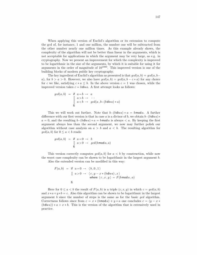
147

When applying this version of Euclid’s algorithm or its extension to computethe gcd of, for instance, 1 and one million, the number one will be subtracted fromthe other number nearly one million times. As this example already shows, thecomplexity of the algorithm will not be better than linear in the arguments, which isnot acceptable for applications in which the argument may be very large, as e.g. incryptography. Now we present an improvement for which the complexity is improvedto be logarithmic in the size of the arguments, by which it is suitable for using it forarguments in the order of magnitude of 101000. This improved version is one of thebuilding blocks of modern public key cryptography.

The key ingredient of Euclid’s algorithm as presented is that gcd(a, b) = gcd(a, b−a), for b > a > 0. However, we also have gcd(a, b) = gcd(a, b − c ∗ a) for any choicefor c we like, satisfying c ∗ a ≤ b. In the above version c = 1 was chosen, while theimproved version takes c = bdiva. A first attempt looks as follows:

gcd(a, b) = if a= b → a[] a> b → · · ·[] a< b → gcd(a , b−(bdiva) ∗ a)fi

This we will work out further. Note that b−(bdiva) ∗ a = bmoda. A furtherdifference with our first version is that in case a is a divisor of b, we obtain b−(bdiva)∗a = 0, and the resulting b−(bdiva) ∗ a = bmoda is always < a. By keeping the firstargument always less than the second argument, we now may further polish ouralgorithm without case analysis on a > b and a < b. The resulting algorithm forgcd(a, b) for 0 ≤ a < b reads:

gcd(a, b) = if a= 0 → b[] a> 0 → gcd(bmoda, a)fi

This version correctly computes gcd(a, b) for a < b by construction, while nowthe worst case complexity can be shown to be logarithmic in the largest argument b.

Also the extended version can be modified in this way:

F (a, b) = if a= 0 → 〈 b , 0 , 1 〉[] a> 0 → 〈 c , y − x ∗ (bdiva) , x 〉

where 〈 c , x , y 〉 = F (bmoda , a)

fi

Here for 0 ≤ a < b the result of F (a, b) is a triple (c, x, y) in which c = gcd(a, b)and x∗a+y ∗b = c. Also this algorithm can be shown to be logarithmic in the largestargument b since the number of steps is the same as for the basic gcd algorithm.Correctness follows since from c = x ∗ (bmoda) + y ∗ a one concludes c = (y − x ∗(bdiva)) ∗ a + x ∗ b. This is the version of the algorithm that is extensively used inpractice.

148

To get a feeling how the algorithm works we apply it by hand to compute valuesx, y satisfying 73x + 87y = 1 = gcd(73, 87). In order to compute F (73, 87) by thealgorithm we have to compute F (14, 73) since 87mod73 = 14, for which we have tocompute F (3, 14), and so on, until we arrive at F (0, 1) = (1, 0, 1). In fact executingthe algorithm corresponds to filling the following table:

a b x y c = x ∗ a+ y ∗ b73 87 31 −26 114 73 −26 5 13 14 5 −1 12 3 −1 1 11 2 1 0 10 1 0 1 1

Here first the columns for a and b are filled from top to bottom. Then in the lastline x = 0 and y = 1 is filled, yielding c = x ∗ a+ y ∗ b = 1. Next the values for x andy are filled from bottom to top in such a way that for every line x∗a+y ∗ b = 1 holds:according to the algorithm this is done by giving y the value of x from the line below,and giving x the value y − x ∗ (bdiva). At the end we fill the first line by x = 31 andy = −26, indeed satisfying the required property 73∗31+87∗(−26) = 1 = gcd(73, 87).

7.5 The prime numbers

In this section we study the set N+2 of multiples, which are the natural numbersfrom 2 onwards. As we have seen, every integer, and, hence, also every multiple isdivisible by 1 and by itself. A multiple with the property that it is not divisible byany other number is called a prime (number).

7.17 Definition. A prime is a multiple that is divisible by 1 and itself only.2

If we would not restrict ourselves to multiples but to positive naturals instead, 1would be a prime too, according to this definition. There are sound, technical reasons,however, not to consider 1 as a prime, which is why we define the primes as a subsetof the multiples. So, the smallest prime is 2 .

7.18 Example. The primes less than 100 are: 2 , 3 , 5 , 7 , 11 , 13 , 17 , 19 , 23 , 29 , 31 , 37 , 4143 , 47 , 53 , 59 , 61 , 67 , 71 , 73 , 79 , 83 , 89 , 97 . Notice that 2 is even and that it is theonly even prime.2

The following lemma expresses that every multiple is divisible by at least one prime.If we would have allowed 1 as a prime number this lemma would have been void.

7.19 Lemma. For every a∈N+2 a prime p exists such that p |a .

Proof. By Mathematical Induction on a . Firstly, if a is a prime then a is a prime

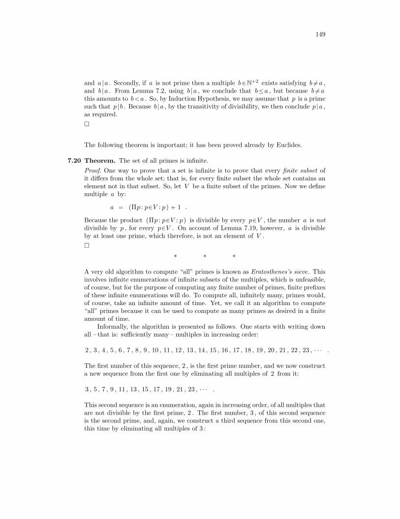
149

and a |a . Secondly, if a is not prime then a multiple b∈N+2 exists satisfying b 6= a ,and b |a . From Lemma 7.2, using b |a , we conclude that b≤ a , but because b 6= athis amounts to b< a . So, by Induction Hypothesis, we may assume that p is a primesuch that p |b . Because b |a , by the transitivity of divisibility, we then conclude p |a ,as required.

The following theorem is important; it has been proved already by Euclides.

7.20 Theorem. The set of all primes is infinite.Proof. One way to prove that a set is infinite is to prove that every finite subset ofit differs from the whole set; that is, for every finite subset the whole set contains anelement not in that subset. So, let V be a finite subset of the primes. Now we definemultiple a by:

a = (Πp : p∈V : p ) + 1 .

Because the product (Πp : p∈V : p ) is divisible by every p∈V , the number a is notdivisible by p , for every p∈V . On account of Lemma 7.19, however, a is divisibleby at least one prime, which therefore, is not an element of V .

* * *

A very old algorithm to compute “all” primes is known as Eratosthenes’s sieve. Thisinvolves infinite enumerations of infinite subsets of the multiples, which is unfeasible,of course, but for the purpose of computing any finite number of primes, finite prefixesof these infinite enumerations will do. To compute all, infinitely many, primes would,of course, take an infinite amount of time. Yet, we call it an algorithm to compute“all” primes because it can be used to compute as many primes as desired in a finiteamount of time.

Informally, the algorithm is presented as follows. One starts with writing downall – that is: sufficiently many – multiples in increasing order:

2 , 3 , 4 , 5 , 6 , 7 , 8 , 9 , 10 , 11 , 12 , 13 , 14 , 15 , 16 , 17 , 18 , 19 , 20 , 21 , 22 , 23 , · · · .

The first number of this sequence, 2 , is the first prime number, and we now constructa new sequence from the first one by eliminating all multiples of 2 from it:

3 , 5 , 7 , 9 , 11 , 13 , 15 , 17 , 19 , 21 , 23 , · · · .

This second sequence is an enumeration, again in increasing order, of all multiples thatare not divisible by the first prime, 2 . The first number, 3 , of this second sequenceis the second prime, and, again, we construct a third sequence from this second one,this time by eliminating all multiples of 3 :

150

5 , 7 , 11 , 13 , 17 , 19 , 23 , · · · .

This sequence contains all multiples that are not divisible by either 2 or 3 ; its firstelement, 5 , is the next prime number, which is the smallest prime that is larger than2 and 3 . And so on. . .

The general properties on account of which this algorithm is correct are easilyformulated. After n steps, for some n∈N , a sequence is obtained that contains, inincreasing order, all multiples that are not divisible by the smallest n prime numbers.The first number of this sequence then, because the sequence is increasing, is itsminimum, and it can be proved that this minimum is the next prime, that is, thesmallest prime number exceeding the smallest n prime numbers. By eliminating allmultiples of this next prime the next sequence is obtained, containing all multiplesnot divisible by the first n+1 primes.

* * *

We have seen that the set of primes is infinite, but we may still ask for the densityof the primes; that is, for any given multiple n we may ask how many primes areless than n . Because the number of potential divisors of n increases with n , thelikelihood – not in the mathematical meaning of the word – that an arbitrary numberis prime may be expected to decrease with increasing numbers.

The, so-called, Prime Number Theorem states that the number of primes less thann is approximately n/ ln(n) . This formula really gives an approximation only; forexample, the number of primes less than 109 equals 50 847 534 , whereas 109/ ln(109)is 48 254 942 (rounded). An elementary proof of the Prime Number Theorem has beenconstructed by the famous Hungarian mathematician Pal Erdos.

The greatest common divisor of a prime p and a positive natural a can haveonly one out of two possible values: either p |a and then gcd(p, a) = p , or ¬ (p |a)and then gcd(p, a) = 1 . An important consequence of this is the following lemma.

7.21 Lemma. For every prime p and for all a, b∈N+ : p | (a∗b) ⇒ p |a ∨ p |b .

Proof. By distinguishing the cases p |a and ¬ (p |a) and, for the latter case, usingLemma 7.15 and gcd(a, p) = 1 if ¬ (p |a) .

7.22 Lemma. If p, q are distinct prime numbers and k ≥ 0, then q is not a divisor of pk.

Proof. Induction on k. For k = 0 clearly q is not a divisor of pk = p0 = 1. Fork > 0 we write pk = p ∗ pk−1. If q |p ∗ pk−1 then by Lemma 7.15 and gcd(p, q) = 1 weconclude q |pk−1, contradicting the induction hypothesis.

The following theorem is known as the Unique Prime Factorization Theorem.Just like we write Σ for summation, we write Π for product. We even take infinite

151

products over all prime numbers as long as all but finitely many are equal to 1: thenthe meaning of the product is the product of the remaining finitely many arguments.

7.23 Theorem. Every positive natural a∈N+ satisfies

a =∏

p primepk(p,a)

in which k(p, a) is the largest number k such that pk |a, for every prime number p.

Proof. We apply induction on a. For a = 1 we have k(p, a) = 0 for all primenumbers, indeed yielding 1 = Πp primep

k(p,1).For a > 1 by Lemma 7.19 a prime q exists such that q |a. We will apply the

induction hypothesis on a/q, yielding a/q = Πp primepk(p,a/q), and we will compare

k(p, a/q) with k(p, a) for all primes p. Since qk(q,a/q) |a/q but not qk(q,a/q)+1 |a/q, weobtain qk(q,a/q)+1 |a but not qk(q,a/q)+2 |a, so k(q, a) = k(q, a/q) + 1.

Next let p be any prime number unequal to q and k any number > 0. We willprove pk |a if and only if pk |a/q. If pk |a/q then a/q = b ∗ pk for some b, yieldinga = pk ∗ (b ∗ q), so pk |a. Conversely let pk |a. Then a = b ∗ pk for some b. Since q |abut not q |pk (by Lemma 7.22), by Lemma 7.21 we conclude q |b, so b = q ∗ c for somec. From a = b∗pk = q ∗ c∗pk we conclude a/q = c∗pk, so pk |a/q. So we have provedpk |a if and only if pk |a/q, so k(p, a) = k(p, a/q).

Combining these results yields

a = q ∗ (a/q)= q ∗

∏p prime p

k(p,a/q) (induction hypothesis)= q ∗ qk(q,a/q) ∗

∏p prime,p6=q p

k(p,a/q) (splitting product)= qk(q,a) ∗

∏p prime,p6=q p

k(p,a) (above observations)=

∏p prime p

k(p,a) (combine product),

concluding the proof.

If a =∏

p prime pk(p,a) and b =

∏p prime p

k(p,b), then it is easily checked thata |b if and only if k(p, a) ≤ k(p, b for all prime numbers p. As a consequence we obtain

gcd(a, b) =∏

p primepmin(k(p,a),k(p,b)).

For instance, 6! = 2 ∗ 3 ∗ 4 ∗ 5 ∗ 6 = 24 ∗ 32 ∗ 51 ∗ 70 and(

83

)= 6 ∗ 7 ∗ 8/(3!) =

23 ∗ 30 ∗ 50 ∗ 71, so gcd(6!,(

83

)) = 23 ∗ 30 ∗ 50 ∗ 70 = 8.

Apart from the Greatest Common Divisor ( gcd ) of two numbers a, b > 0 onemay also consider the Least Common Multiple ( lcm ): lcm(a, b) is defined to be the

152

least number n such that a |n and b |n. Such a number n with a |n and b |n alwaysexists since a ∗ b satisfies the requirements, but a ∗ b does not need to be the smallestone. In fact, from the above observations one easily checks

lcm(a, b) =∏

p primepmax(k(p,a),k(p,b)).

Since for any two numbers k, k′ we have max(k, k′) + min(k, k′) = k + k′, we obtain

gcd(a, b) ∗ lcm(a, b) =∏

p primepmin(k(p,a),k(p,b))+max(k(p,a),k(p,b))

=∏

p primepk(p,a)+k(p,b) = a ∗ b

for all a, b > 0.From these characterizations of gcd and lcm one easily derives that

c |a ∧ c |b ⇔ c |gcd(a, b)

and

a |c ∧ b |c ⇔ gcd(a, b) |c

for all numbers a, b, c > 0. As a consequence, we obtain that (N+, | ) is a lattice, inwhich gcd corresponds to the infimum and lcm corresponds to the supremum.

7.6 Modular Arithmetic

7.6.1 Congruence relations

Almost everybody probably knows that the product of two even integers is even, andthat the product of two odd integers is odd. Also, the sum of two even integers is eventoo, and even the sum of two odd numbers is even. The point is that, apparently,whether the result of an operation, like addition or multiplication, is even or odd onlydepends on whether the arguments of the operation are even or odd.

The proposition that integer “x is even” is equivalent to “x is divisible by 2 ”,which in turn is equivalent to xmod2 = 0 ; similarly, the proposition “x is odd”is equivalent to xmod2 = 1 . That the property “being even” of the sum of twointegers only depends on the “being even” of these two numbers know means that(x+y) mod 2 only depends on xmod2 and ymod2 (and not on xdiv2 or y div2 ).In formula this is rendered as:

(18) (x+y) mod 2 = (xmod2 + ymod2) mod 2 , for all x, y ∈Z .

Properties like these are not specific for 2 as a divisor: similar properties hold forall positive divisors. From the chapter on relations we recall that, for every functionof type B→V , the relation, on its domain B , “having the same function value”

153

is an equivalence relation. For any fixed d∈N+ , the function (modd ) that mapsevery x∈Z to xmodd has type Z→ [ 0 . . d ) . This function induces an equivalencerelation, on Z , of “having the same remainder when divided by d ”. This relationpartitions Z into d different (and, as always, disjoint) equivalence classes, namelyone for every value of the function (modd ) : the equivalence class corresponding toa∈ [ 0 . . d ) is the set

x∈Z | xmodd= a ,

which can also be formulated as:

q ∗ d+a | q∈Z .

In particular, of course, a ∈ x∈Z | xmodd= a , because amodd = a , for everya∈ [ 0 . . d ) .

Now properties similar to (18) also hold in this case; that is, we now have:

(19) (x+y) mod d = (xmodd + ymodd ) mod d , for all x, y ∈Z .

A similar property holds for subtraction and multiplication:

(20) (x ∗ y) mod d = (xmodd ∗ ymodd ) mod d , for all x, y ∈Z .

A consequence of propositions like (19) and (20) is that equivalence is preserved un-der arithmetic operations like addition and multiplication. Using (19) , for instance,we can now derive, for all x, y, z ∈Z :

(21) xmodd = ymodd ⇒ (x+z) mod d = (y+z) mod d .

An equivalence relation that is preserved under a given set of operations is calleda congruence relation. In our case, the relation “having the same remainder whendivided by d ” is congruent with the operations addition, subtraction, and multi-plication. Conversely, we also say that the operations addition, subtraction, andmultiplication are compatible with the relation.

Notation: According to mathematical tradition, the fact that x and y arecongruent modulo d is often denoted as:

x = y (mod d) .

This notation is somewhat awkward, though, because it is not very clearwhat the scope is of the suffix “ (mod d) ”. Apparently, its scope extendsover the complete equality textually preceding it; that is, if we would usesome sort of brackets to delineate the scope of “(mod d)” more explicitly,we should write something like:

|[ x = y (mod d) ]| .

Because the relation is a congruence relation and because it is not the same assheer equality, although it resembles it, it seems better to denote the relationas an infix symbol resembling but different from “ = ”. For example, the

154

symbol “ =mod d ” would be appropriate, as the subscript explicitly indicatesthe nature of the congruence. In this text we will abbreviate this to “ =d ”;so, by definition we now have, for all d∈N+ and x, y ∈Z :

x =d y ⇔ xmodd = ymodd .

For example, congruence property (21) can now be rendered as, for allx, y, z ∈Z :

x =d y ⇒ x+z =d y+z .2

Other algebraic properties are compatible with congruence modulo d too. The num-bers 0 and 1 , for instance, are the identity elements of addition and multiplication,respectively, and this remains so under congruence. In addition, the property that0 is a zero-element of multiplication – that is: 0 ∗x = 0 – is retained. Finally, thatmultiplication distributes over addition remains true as well.

For any given d∈N+ we can now define binary operations ⊕ and ⊗ , say, by,for all x, y ∈Z :

x⊕ y = (x+y) mod d , and:

x⊗ y = (x ∗ y) mod d , and:

(If we would be very strict we should make the dependence on d explicit by writing⊕d and ⊗d .) Now ⊕ and ⊗ have type [ 0 . . d )×[ 0 . . d )→ [ 0 . . d ) and with theseoperators various algebraic structures can be formed, which we mention here withoutfurther elaboration or proofs.

7.24 Theorem. For all d∈N+ :

(a) ( [ 0 . . d ) ,⊕ , 0) is a group.

(b) ( [ 0 . . d ) ,⊗ , 1) is a monoid but not a group.

(c) ( [ 1 . . d ) ,⊗ , 1) is a group if and only if d is prime.

Proof. Most monoid and group axioms are checked straightforwardly, where 0 is theidentity of ⊕ and 1 is the identity of ⊗.

In (b) it is not a group since 0 has no inverse: there is no x ∈ [ 0 . . d ) such thatx⊗0 = 1.

For (c) we also have to check that ⊗ is well-defined, that is, if a, b ∈ [ 1 . . d ) thena⊗b should be in [ 1 . . d ) too, that is, a ∗ bmodd ∈ [ 1 . . d ). If d is not a prime, thisis not the case since we can write d = a ∗ b for a, b ∈ [ 1 . . d ), by which a ∗ bmodd =0 6∈ [ 1 . . d ). If d is prime then well-definedness holds since if a, b ∈ [ 1 . . d ) thena ∗ bmodd 6= 0 due to Lemma 7.21. It remains to prove that every a ∈ [ 1 . . d ) has aninverse. Observe that gcd(a, d) = 1. By the extended Euclid’s algorithm then thereexist x, y such that x ∗ a+ y ∗ d = 1. Hence x ∗ amodd = 1, so x is the inverse of a.

155

7.6.2 An application: the nine and eleven tests

A technique that was commonly applied to verify manual calculations is the, so-called,nine test . This is based on the property that, in our decimal number representation,the remainder of a number when divided by 9 can be easily calculated: it equalsthe remainder of the sum of the number’s digits modulo 9 . As the sum of the digitsof a number usually is much smaller than the number itself, the problem has beenreduced. This process is repeated until a number is obtained that is less than 10 :this last number, then, is the remainder of the original number modulo 9 , exceptwhen it is 9 in which case the remainder is 0 , of course.

For example, the sum of the digits of the number 123456789 equals 45 , and thesum of the digits of 45 is 9 . Hence, the remainder of 123456789 modulo 9 is 0 .

Now to verify a calculation, for instance the addition or multiplication of twolarge numbers, one calculates the remainders modulo 9 of both numbers and of theresult of the calculation, and one performs the same operation, modulo 9 , to theseremainders. If the results match we can be pretty confident that our calculation wascorrect, although we do not have certainty, of course. But, if the results do not matchwe certainly have made an error!

* * *

The property that the remainder modulo 9 of a number equals the remainder modulo9 of the sum of the digits of that number’s decimal representation is based on theobservation that 10mod9 = 1 . Now we have that a number like, for instance, 1437is equal to 143 ∗ 10 + 7 . Therefore, we have:

1437 mod 9

= above property (143 ∗ 10+7) mod 9

= 10 = 9+1 (143 ∗ 9+143 ∗ 1+7) mod 9

= mod over + ; multiples of 9 may be discarded and 7mod9 = 7 (143mod9 + 7) mod 9 .

This calculation shows that 1437 mod 9 is equal to 143 mod 9 plus 7 , modulo 9 ;if now, by Induction Hypothesis, 143 mod 9 is equal to the sum, modulo 9 , of thedigits of 143 then 1437 mod 9 also is equal to the sum of its digits, modulo 9 .

* * *

In general, the decimal representation of natural numbers can be defined in a recursiveway, as follows. A sequence of n decimal digits “ dn−1 · · · d2d1d0 ” represents thenatural number d0 if n= 1 : in this case the sequence just is a single digit, “ d0 ”. Ifn≥ 2 , the number represented by the sequence is equal to the number representedby the sequence of n−1 digits “ dn−1 · · · d2d1 ” times 10 plus d0 .

156

By means of this recursive definition it can be proved, by Mathematical Induc-tion, of course, that the number represented by a sequence of decimal digits and thesum of these digits are congruent modulo 9 . By means of the recursive definitionit also is possible to prove that the number represented by the sequence of digits“ dn−1 · · · d2d1d0 ” is equal to:

(Σi : 0≤i<n : di ∗ 10i ) ,

but in most cases the recursive definition is more manageable than this expression.

* * *

In a very similar, albeit slightly more complicated way we observe that 10 is congruentto −1 modulo 11 , and that 100mod11 is equal to 1 . This is the basis of the eleventest : the remainder of a natural number modulo 11 is equal to the remainder modulo11 of the sum of the digits of that number’s decimal representation, but here thedigits are added with alternating signs, starting at the least-significant digit witha positive sign. The number 123456789 , for example, is congruent modulo 11 to:+9−8+7−6+5−4+3−2+1 , which equals 5 .

As was the case with the nine test, the eleven test can be used to “verify” theresults of calculations.

7.7 Fermat’s little theorem

We prove the following theorem which is known as “Fermat’s little theorem”.

7.25 Theorem. For every prime number p and for every a∈N+ we have:

¬ (p |a) ⇒ ap−1 mod p = 1 .

Proof. Let p be a prime and let a∈N+ . Assume ¬ (p |a) ; this is equivalent toamodp 6= 0 , so we have: 1 ≤ amodp < p ; that is, amodp ∈ [ 1 . . p ) . For the sake ofbrevity, we define b = amodp . Now we have that ap−1 mod p is equal to bp−1 , whereb ∈ [ 1 . . p ) and bp−1 is to be interpreted in terms of ⊗ -operations, instead of ∗ .Hence, we also have bp−1 ∈ [ 1 . . p ) .

By Theorem 7.24, part (c), we have that ( [ 1 . . p ) ,⊗ , 1) is a group, because p isprime. The set bi | 0≤i together with ⊗ and 1 is the subgroup of ( [ 1 . . p ) ,⊗ , 1)generated by b . Because the whole group is finite, of size p−1 , so is this subgroup.Therefore, a number n∈N+ exists such that bn = 1 and bi 6= 1 , for all i : 1≤i<n .Then we have: bi | 0≤i = bi | 0≤i<n , and n is the size of this set.

On account of Lagrange’s Theorem we conclude n | (p−1) . So, let z ∈N satisfyp−1 = z ∗n . Now we derive:

ap−1 mod p

= as observed above bp−1

= definition of z

157

bz∗n

= property of exponentiation (bn)z

= definition of n 1z

= 1 is the identity of ⊗ 1

7.8 Cryptography: the RSA algorithm

We conclude this chapter with a practical application of the theory, namely in thearea of cryptography , which is the art of transmitting messages in a secure way, suchthat these messages cannot be read by anyone else than the intended receiver. For thispurpose the messages are encrypted in such a way that they become unintelligible,except for the intended receiver who is the only one able to decipher the messages.

The algorithms for encryption and decryption themselves usually are not keptsecret, but the parameters used in the process are. In cryptography such parametersusually are called keys.

Here we discuss the, so-called, RSA-algorithm, named after its inventors: Rivest,Shamir, and Adleman. This is an example of a so-called public key system. Thismeans that the keys needed for encryption and decryption are chosen by the receiverof the messages, and the receiver makes the encryption key publicly known: everybodywho wishes to send a message to this particular receiver now can use this publicencryption key. The security of this arrangement is based on the assumption that it is(virtually) impossible to infer the (secret) decryption key from the (public) encryptionkey.

In older encryption schemes the encryption and decryption keys used to be chosenby the sender of the messages, and the sender now was faced with the problem howto communicate the decryption key to the intended receiver(s) in a secure way. In apublic key system this difficulty is avoided.

The security of the RSA-algorithm rest on the assumption that it is very hardto factorize very large numbers into their prime factors. Here “very large numbers”means: numbers the decimal representation of which comprises several hundreds ofdigits.

* * *

The RSA-algorithm is based in two very large prime numbers p and q . Let n = p ∗ q .Let a be any positive natural number not divisible by p or q. Then, by Fermat’s littletheorem, we have:

ap−1 mod p = 1 ∧ aq−1 mod q = 1 .

158

From this it follows that we also have, because 1p−1 and 1q−1 are equal to 1 :

a(p−1)∗(q−1) mod p = 1 ∧ a(p−1)∗(q−1) mod q = 1 .

So a(p−1)∗(q−1) − 1 is divisible by both p and q, so also by p ∗ q since p and q areprime. So

(22) a(p−1)∗(q−1) mod n = 1 .

For every k ≥ 0 we have 1k = 1, so

ak∗(p−1)∗(q−1)+1 modn = a.

Now encryption of a secret message works as follows. Choose an encryptionnumber e with gcd(e, (p − 1) ∗ (q − 1)) = 1. Represent the message by a numberM , with 0 < M < n, not divisible by p or q, for instance, the number of whichthe binary representation is the sequence of bits of the message. Now the encryptedmessage is Me modn. By the extended Euclid’s algorithm find numbers d, k such thatd ∗ e− k ∗ (p− 1) ∗ (q − 1) = 1. Now we obtain

(Me)d modn = Md∗e modn = Mk∗(p−1)∗(q−1)+1 modn = M.

If some person A wants to receive a secret message from B then A chooses twolarge prime numbers p, q, computes n = p ∗ q, chooses a corresponding value e andsends n, e to B in a non-safe way, by which also intruders may know n, e. Next Btakes its secret message M , and computes M ′ = Me modn (encryption), and sendsM ′ to A in a non-safe way, by which also intruders may know M ′. Now A can decryptM ′ to M by computing d as presented above, and computing M ′d modn = M . Thecrucial point is that knowledge of both p and q are required to do this computation,so intruders that may know n, e,M ′ have no clue how to construct the secret messageM . Safety and feasibility of this approach depend on the following assumptions:

• if you know n = p ∗ q, there is no feasible way to establish p and q,

• the extended Euclid’s algorithm is feasible, even for n having thousands of digits,

• for numbers a, b, n of thousands of digits each, computation of ab modn is feasi-ble.

For computing ab modn clearly ab should not be computed since this number cannever be stored: probably the number of digits of this number exceeds the number ofatoms in the universe. Also not b times a multiplication with a should be executed,since b is far too large. But by carefully combining squaring and multiplying by a,and reducing all intermediate result modulo n, computing ab modn is feasible.

Although there is no formal proof that when knowing n, e,M ′ it is not feasible tocompute M , it has turned out to be safe in practice. The RSA algorithm was proposedby Rivest, Shamir and Adleman in 1977. In that time taking prime numbers of 100digits was safe. However, both to increasing computational power and improvedalgorithms the approach is currently not safe any more for 100 digits, but for 1000digits it is.

159

7.9 Exercises

1. Let a, d∈Z and d 6= 0 . Assuming that a is divisible by d , prove that the valueq satisfying a = q ∗ d is unique.

2. (a) What are the divisors of 1 ? Prove the correctness of your answer.

(b) Prove (∀a, d : a∈Z ∧ d∈N+2 : d |a ⇒ ¬ (d | (a+1)) ) .

(c) Prove (∀a, b, d : a, b∈Z ∧ d 6= 0 : d |a ∨ d |b ⇒ d | (a∗b) ) .

(d) Give a simple counter-example illustrating that Lemma 7.21 does not holdif p is not prime, for every p∈N+2 .

3. Prove the following properties of div and mod , using Definition 7.5 ; it is giventhat d∈N+ and that a, b, x∈Z :

(a) 0≤ a< d ⇔ (amodd) = a

(b) 0≤ a< d ⇔ (adivd) = 0

(c) 0≤ a ⇔ 0≤ adivd

(d) (a+d) modd = amodd

(e) (a+d) divd = (adivd) +1

(f) (a+x ∗d) modd = amodd

(g) (a+x ∗d) divd = (adivd) +x

(h) (amodd) modd = amodd

(i) (amodd) divd = 0

(j) (a+b) modd = (amodd + bmodd ) mod d

(k) (a+b) divd = (adivd) + (bdivd) + (amodd+ bmodd) divd

(l) Give (simple) counter examples illustrating that (a+b) modd is not nec-essarily equal to amodd+ bmodd , and that (a+b) divd is not necessarilyequal to adivd+ bdivd .

(m) (a ∗ b) modd = ( (amodd) ∗ (bmodd) ) mod d

(n) amodd = 0 ⇔ d |a(o) amodd = 0 ⇔ adivd = a/d

(p) 1≤a ⇔ adivd< a , provided that 2≤ d

(q) amodd = bmodd ⇔ (a−b) mod d = 0

(r) Determine (−1)divd en (−1)modd

4. Given are c, d∈N+ . Prove that for all a∈Z :(a ∗ d) mod (c ∗ d) = (amodc) ∗ d and:

(a ∗ d) div (c ∗ d) = adivc .

5. (a) Determine the gcd of the numbers 112 and 280 .

160

(b) Determine numbers x and y satisfying: x∗112 + y∗280 = gcd (112 , 280) .

6. Determine, by hand, all prime numbers between 100 and 200 .

7. Prove that x ∗ (x+1) ∗ (x+2) is divisible by 6 , for all x∈Z .

8. Prove that (x2−1)mod8 ∈ 0 , 3 , 7 , for all x∈Z .

9. Resolve 8!− 3 ∗ 7! into prime factors.

10. Determine the lcm of the numbers 1500000021 and 3000000045 .

11. Find integers x, y such that 100 ∗ x+ 17 ∗ y = 1.

12. Find an integer x such that 0 < x < 144 and 83 ∗ xmod144 = 1.

13. Are there integers x, y such that 111 ∗ x + 27 ∗ y = 5? If so, find them, if not,prove this.

14. We consider the number whose decimal representation consists of 38 digits 1 .We call this number X .

(a) Give a, formally correct, mathematical expression for X .

(b) What is the remainder of the division of x by 9 ?

(c) What is the remainder of the division of x by 11 ?

(d) What is the remainder of the division of x by 99 ?

15. Determine all values x∈Z satisfying both: x= 2 (mod 11) and: x= 3 (mod 23) .

16. Resolve(

175

)into prime factors.

17. Determine the gcd and lcm of(

175

)and

(184

).

18. Prove that (n+1) ∗ (n+2) ∗ · · · ∗ (n+k) is divisible by k! , for all n, k ∈N .

19. Prove that a natural number is divisible by 4 if and only if, in the representationof that number in base 17 , the sum of the digits is divisible by 4 .

20. We know that 37 ∗ 43 = 1591 . Determine e∈N in such a way that, for all m∈Z ,we have: m127∗e =1591 m .

21. Represent the number 1000 in base m , for every m ∈ 2 , 3 , 4 , 5 , 6 , 7 , 8 , 9 , 10 .

22. What is the period of the recurring decimal fraction that represents 1/1001001 ?

23. For a natural number n > 10 it is given that 2n modn = 5. Prove that n is nota prime number.

24. Determine all prime numbers p with the property that 33 ∗ p+ 1 is a square.

161

25. A given number requires 10 (ternary) digits for its ternary representation. Howmany digits are needed to represent this number in the decimal system?

26. For natural numbers a, b prove that a | b if and only if D(a) ⊆ D(b).