discrete time markov chains, limiting distribution and … · classification of markov chain...
TRANSCRIPT

Discrete Time Markov Chains, LimitingDistribution and Classification
Bo Friis Nielsen1
1DTU Informatics
02407 Stochastic Processes 3, September 19 2017
Bo Friis Nielsen Limiting Distribution and Classification

Discrete time Markov chains
Today:
I Discrete time Markov chains - invariant probabilitydistribution
I Classification of statesI Classification of chains
Next week
I Poisson process
Two weeks from now
I Birth- and Death Processes
Bo Friis Nielsen Limiting Distribution and Classification

Regular Transition Probability Matrices
P =∣∣∣∣Pij
∣∣∣∣ , 0 ≤ i , j ≤ N
Regular: If Pk > 0 for some kIn that case limn→∞ P(n)
ij = πj
Theorem 4.1 (Page 168) let P be a regular transitionprobability matrix on the states 0,1, . . . ,N. Then the limitingdistribution π = (π0, π1, πN) is the unique nonnegative solutionof the equations
πj =N∑
k=0
πkPij , π = πP
N∑k=0
πk = 1, π1 = 1
Bo Friis Nielsen Limiting Distribution and Classification

Interpretation of πj ’s
I Limiting probabilities limn→∞ P(n)ij = πj
I Long term averages limn→∞11∑m
n=1 P(n)ij = πj
I Stationary distribution π = πP
Bo Friis Nielsen Limiting Distribution and Classification

Interpretation of πj ’s
I Limiting probabilities limn→∞ P(n)ij = πj
I Long term averages limn→∞11∑m
n=1 P(n)ij = πj
I Stationary distribution π = πP
Bo Friis Nielsen Limiting Distribution and Classification

Interpretation of πj ’s
I Limiting probabilities limn→∞ P(n)ij = πj
I Long term averages limn→∞11∑m
n=1 P(n)ij = πj
I Stationary distribution π = πP
Bo Friis Nielsen Limiting Distribution and Classification

Interpretation of πj ’s
I Limiting probabilities limn→∞ P(n)ij = πj
I Long term averages limn→∞11∑m
n=1 P(n)ij = πj
I Stationary distribution π = πP
Bo Friis Nielsen Limiting Distribution and Classification

A Social Mobility Example
Son’s ClassLower Middle Upper
Lower 0.40 0.50 0.10Father’s Middle 0.05 0.70 0.25Class Upper 0.05 0.50 0.45
P8 =
∣∣∣∣∣∣∣∣∣∣∣∣
0.0772 0.6250 0.29780.0769 0.6250 0.29810.0769 0.6250 0.2981
∣∣∣∣∣∣∣∣∣∣∣∣
π0 = 0.40π0 + 0.05π1 + 0.05π2
π1 = 0.50π0 + 0.70π1 + 0.50π2
π2 = 0.10π0 + 0.25π1 + 0.45π2
1 = π0 + π1 + π2
Bo Friis Nielsen Limiting Distribution and Classification

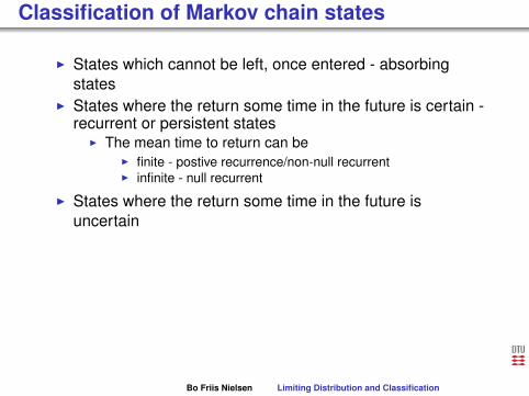
Classification of Markov chain states
I States which cannot be left, once entered - absorbingstates
I States where the return some time in the future is certain -recurrent or persistent states
I The mean time to return can beI finite - postive recurrence/non-null recurrentI infinite - null recurrent
I States where the return some time in the future isuncertain - transient states
I States which can only be visited at certain time epochs -periodic states
Bo Friis Nielsen Limiting Distribution and Classification

Classification of Markov chain states
I States which cannot be left, once entered
- absorbingstates
I States where the return some time in the future is certain -recurrent or persistent states
I The mean time to return can beI finite - postive recurrence/non-null recurrentI infinite - null recurrent
I States where the return some time in the future isuncertain - transient states
I States which can only be visited at certain time epochs -periodic states
Bo Friis Nielsen Limiting Distribution and Classification

Classification of Markov chain states
I States which cannot be left, once entered - absorbingstates
I States where the return some time in the future is certain -recurrent or persistent states
I The mean time to return can beI finite - postive recurrence/non-null recurrentI infinite - null recurrent
I States where the return some time in the future isuncertain - transient states
I States which can only be visited at certain time epochs -periodic states
Bo Friis Nielsen Limiting Distribution and Classification

Classification of Markov chain states
I States which cannot be left, once entered - absorbingstates
I States where the return some time in the future is certain
-recurrent or persistent states
I The mean time to return can beI finite - postive recurrence/non-null recurrentI infinite - null recurrent
I States where the return some time in the future isuncertain - transient states
I States which can only be visited at certain time epochs -periodic states
Bo Friis Nielsen Limiting Distribution and Classification

Classification of Markov chain states
I States which cannot be left, once entered - absorbingstates
I States where the return some time in the future is certain -recurrent or persistent states
I The mean time to return can beI finite - postive recurrence/non-null recurrentI infinite - null recurrent
I States where the return some time in the future isuncertain - transient states
I States which can only be visited at certain time epochs -periodic states
Bo Friis Nielsen Limiting Distribution and Classification

Classification of Markov chain states
I States which cannot be left, once entered - absorbingstates
I States where the return some time in the future is certain -recurrent or persistent states
I The mean time to return can be
I finite - postive recurrence/non-null recurrentI infinite - null recurrent
I States where the return some time in the future isuncertain - transient states
I States which can only be visited at certain time epochs -periodic states
Bo Friis Nielsen Limiting Distribution and Classification

Classification of Markov chain states
I States which cannot be left, once entered - absorbingstates
I States where the return some time in the future is certain -recurrent or persistent states
I The mean time to return can beI finite
- postive recurrence/non-null recurrentI infinite - null recurrent
I States where the return some time in the future isuncertain - transient states
I States which can only be visited at certain time epochs -periodic states
Bo Friis Nielsen Limiting Distribution and Classification

Classification of Markov chain states
I States which cannot be left, once entered - absorbingstates
I States where the return some time in the future is certain -recurrent or persistent states
I The mean time to return can beI finite - postive recurrence/non-null recurrent
I infinite - null recurrent
I States where the return some time in the future isuncertain - transient states
I States which can only be visited at certain time epochs -periodic states
Bo Friis Nielsen Limiting Distribution and Classification

Classification of Markov chain states
I States which cannot be left, once entered - absorbingstates
I States where the return some time in the future is certain -recurrent or persistent states
I The mean time to return can beI finite - postive recurrence/non-null recurrentI infinite
- null recurrent
I States where the return some time in the future isuncertain - transient states
I States which can only be visited at certain time epochs -periodic states
Bo Friis Nielsen Limiting Distribution and Classification

Classification of Markov chain states
I States which cannot be left, once entered - absorbingstates
I States where the return some time in the future is certain -recurrent or persistent states
I The mean time to return can beI finite - postive recurrence/non-null recurrentI infinite - null recurrent
I States where the return some time in the future isuncertain - transient states
I States which can only be visited at certain time epochs -periodic states
Bo Friis Nielsen Limiting Distribution and Classification
Classification of Markov chain states
I States which cannot be left, once entered - absorbingstates
I States where the return some time in the future is certain -recurrent or persistent states
I The mean time to return can beI finite - postive recurrence/non-null recurrentI infinite - null recurrent
I States where the return some time in the future isuncertain
- transient statesI States which can only be visited at certain time epochs -
periodic states
Bo Friis Nielsen Limiting Distribution and Classification

Classification of Markov chain states
I States which cannot be left, once entered - absorbingstates
I States where the return some time in the future is certain -recurrent or persistent states
I The mean time to return can beI finite - postive recurrence/non-null recurrentI infinite - null recurrent
I States where the return some time in the future isuncertain - transient states
I States which can only be visited at certain time epochs -periodic states
Bo Friis Nielsen Limiting Distribution and Classification

Classification of Markov chain states
I States which cannot be left, once entered - absorbingstates
I States where the return some time in the future is certain -recurrent or persistent states
I The mean time to return can beI finite - postive recurrence/non-null recurrentI infinite - null recurrent
I States where the return some time in the future isuncertain - transient states
I States which can only be visited at certain time epochs
-periodic states
Bo Friis Nielsen Limiting Distribution and Classification

Classification of Markov chain states
I States which cannot be left, once entered - absorbingstates
I States where the return some time in the future is certain -recurrent or persistent states
I The mean time to return can beI finite - postive recurrence/non-null recurrentI infinite - null recurrent
I States where the return some time in the future isuncertain - transient states
I States which can only be visited at certain time epochs -periodic states
Bo Friis Nielsen Limiting Distribution and Classification

Classification of States
I j is accessible from i if P(n)ij > 0 for some n
I If j is accessible from i and i is accessible from j we saythat the two states communicate
I Communicating states constitute equivalence classes (anequivalence relation)
I i communicates with j and j communicates with k then iand k communicates
Bo Friis Nielsen Limiting Distribution and Classification

First passage and first return timesWe can formalise the discussion of state classification by use ofa certain class of probability distributions
- first passage timedistributions. Define the first passage probability
f (n)ij = P{X1 6= j ,X2 6= j , . . . ,Xn−1 6= j ,Xn = j |X0 = i}
This is the probability of reaching j for the first time at time nhaving started in i .What is the probability of ever reaching j?
fij =∞∑
n=1
f (n)ij ≤ 1
The probabilities f (n)ij constitiute a probability distribution. Onthe contrary we cannot say anything in general on
∑∞n=1 p(n)
ij(the n-step transition probabilities)
Bo Friis Nielsen Limiting Distribution and Classification

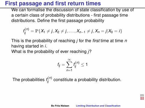
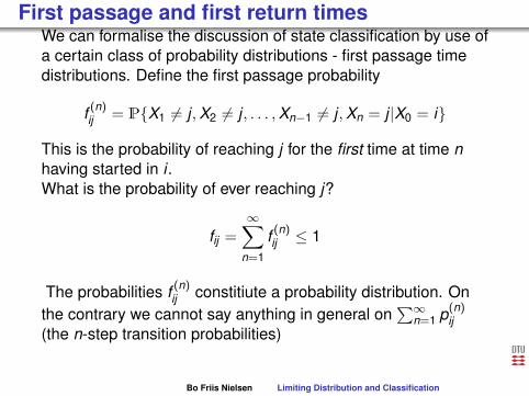
First passage and first return timesWe can formalise the discussion of state classification by use ofa certain class of probability distributions - first passage timedistributions.
Define the first passage probability
f (n)ij = P{X1 6= j ,X2 6= j , . . . ,Xn−1 6= j ,Xn = j |X0 = i}
This is the probability of reaching j for the first time at time nhaving started in i .What is the probability of ever reaching j?
fij =∞∑
n=1
f (n)ij ≤ 1
The probabilities f (n)ij constitiute a probability distribution. Onthe contrary we cannot say anything in general on
∑∞n=1 p(n)
ij(the n-step transition probabilities)
Bo Friis Nielsen Limiting Distribution and Classification

First passage and first return timesWe can formalise the discussion of state classification by use ofa certain class of probability distributions - first passage timedistributions. Define the first passage probability
f (n)ij =
P{X1 6= j ,X2 6= j , . . . ,Xn−1 6= j ,Xn = j |X0 = i}
This is the probability of reaching j for the first time at time nhaving started in i .What is the probability of ever reaching j?
fij =∞∑
n=1
f (n)ij ≤ 1
The probabilities f (n)ij constitiute a probability distribution. Onthe contrary we cannot say anything in general on
∑∞n=1 p(n)
ij(the n-step transition probabilities)
Bo Friis Nielsen Limiting Distribution and Classification

First passage and first return timesWe can formalise the discussion of state classification by use ofa certain class of probability distributions - first passage timedistributions. Define the first passage probability
f (n)ij = P{X1 6= j ,X2 6= j , . . . ,Xn−1 6= j ,Xn = j |X0 = i}
This is the probability of reaching j for the first time at time nhaving started in i .What is the probability of ever reaching j?
fij =∞∑
n=1
f (n)ij ≤ 1
The probabilities f (n)ij constitiute a probability distribution. Onthe contrary we cannot say anything in general on
∑∞n=1 p(n)
ij(the n-step transition probabilities)
Bo Friis Nielsen Limiting Distribution and Classification

First passage and first return timesWe can formalise the discussion of state classification by use ofa certain class of probability distributions - first passage timedistributions. Define the first passage probability
f (n)ij = P{X1 6= j ,X2 6= j , . . . ,Xn−1 6= j ,Xn = j |X0 = i}
This is the probability of reaching j for the first time at time nhaving started in i .
What is the probability of ever reaching j?
fij =∞∑
n=1
f (n)ij ≤ 1
The probabilities f (n)ij constitiute a probability distribution. Onthe contrary we cannot say anything in general on
∑∞n=1 p(n)
ij(the n-step transition probabilities)
Bo Friis Nielsen Limiting Distribution and Classification

First passage and first return timesWe can formalise the discussion of state classification by use ofa certain class of probability distributions - first passage timedistributions. Define the first passage probability
f (n)ij = P{X1 6= j ,X2 6= j , . . . ,Xn−1 6= j ,Xn = j |X0 = i}
This is the probability of reaching j for the first time at time nhaving started in i .What is the probability of ever reaching j?
fij =∞∑
n=1
f (n)ij ≤ 1
The probabilities f (n)ij constitiute a probability distribution. Onthe contrary we cannot say anything in general on
∑∞n=1 p(n)
ij(the n-step transition probabilities)
Bo Friis Nielsen Limiting Distribution and Classification

First passage and first return timesWe can formalise the discussion of state classification by use ofa certain class of probability distributions - first passage timedistributions. Define the first passage probability
f (n)ij = P{X1 6= j ,X2 6= j , . . . ,Xn−1 6= j ,Xn = j |X0 = i}
This is the probability of reaching j for the first time at time nhaving started in i .What is the probability of ever reaching j?
fij
=∞∑
n=1
f (n)ij ≤ 1
The probabilities f (n)ij constitiute a probability distribution. Onthe contrary we cannot say anything in general on
∑∞n=1 p(n)
ij(the n-step transition probabilities)
Bo Friis Nielsen Limiting Distribution and Classification

First passage and first return timesWe can formalise the discussion of state classification by use ofa certain class of probability distributions - first passage timedistributions. Define the first passage probability
f (n)ij = P{X1 6= j ,X2 6= j , . . . ,Xn−1 6= j ,Xn = j |X0 = i}
This is the probability of reaching j for the first time at time nhaving started in i .What is the probability of ever reaching j?
fij =∞∑
n=1
f (n)ij
≤ 1
The probabilities f (n)ij constitiute a probability distribution. Onthe contrary we cannot say anything in general on
∑∞n=1 p(n)
ij(the n-step transition probabilities)
Bo Friis Nielsen Limiting Distribution and Classification

First passage and first return timesWe can formalise the discussion of state classification by use ofa certain class of probability distributions - first passage timedistributions. Define the first passage probability
f (n)ij = P{X1 6= j ,X2 6= j , . . . ,Xn−1 6= j ,Xn = j |X0 = i}
This is the probability of reaching j for the first time at time nhaving started in i .What is the probability of ever reaching j?
fij =∞∑
n=1
f (n)ij ≤ 1
The probabilities f (n)ij constitiute a probability distribution. Onthe contrary we cannot say anything in general on
∑∞n=1 p(n)
ij(the n-step transition probabilities)
Bo Friis Nielsen Limiting Distribution and Classification
First passage and first return timesWe can formalise the discussion of state classification by use ofa certain class of probability distributions - first passage timedistributions. Define the first passage probability
f (n)ij = P{X1 6= j ,X2 6= j , . . . ,Xn−1 6= j ,Xn = j |X0 = i}
This is the probability of reaching j for the first time at time nhaving started in i .What is the probability of ever reaching j?
fij =∞∑
n=1
f (n)ij ≤ 1
The probabilities f (n)ij constitiute a probability distribution.
Onthe contrary we cannot say anything in general on
∑∞n=1 p(n)
ij(the n-step transition probabilities)
Bo Friis Nielsen Limiting Distribution and Classification

First passage and first return timesWe can formalise the discussion of state classification by use ofa certain class of probability distributions - first passage timedistributions. Define the first passage probability
f (n)ij = P{X1 6= j ,X2 6= j , . . . ,Xn−1 6= j ,Xn = j |X0 = i}
This is the probability of reaching j for the first time at time nhaving started in i .What is the probability of ever reaching j?
fij =∞∑
n=1
f (n)ij ≤ 1
The probabilities f (n)ij constitiute a probability distribution. Onthe contrary we cannot say anything in general on
∑∞n=1 p(n)
ij
(the n-step transition probabilities)
Bo Friis Nielsen Limiting Distribution and Classification
First passage and first return timesWe can formalise the discussion of state classification by use ofa certain class of probability distributions - first passage timedistributions. Define the first passage probability
f (n)ij = P{X1 6= j ,X2 6= j , . . . ,Xn−1 6= j ,Xn = j |X0 = i}
This is the probability of reaching j for the first time at time nhaving started in i .What is the probability of ever reaching j?
fij =∞∑
n=1
f (n)ij ≤ 1
The probabilities f (n)ij constitiute a probability distribution. Onthe contrary we cannot say anything in general on
∑∞n=1 p(n)
ij(the n-step transition probabilities)
Bo Friis Nielsen Limiting Distribution and Classification

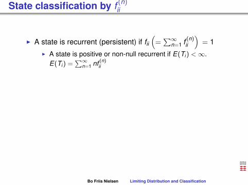
State classification by f (n)ii
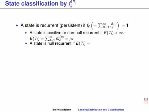
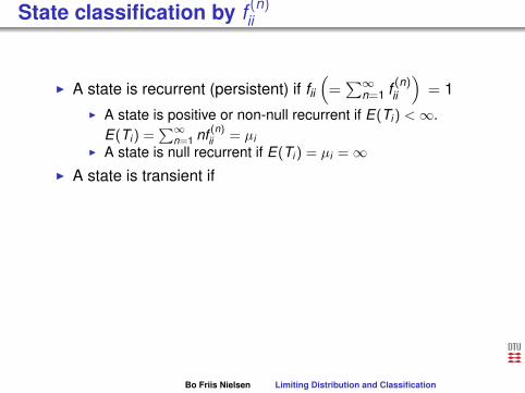
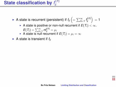
I A state is recurrent (persistent) if fii(=∑∞
n=1 f (n)ii
)= 1
I A state is positive or non-null recurrent if E(Ti) <∞.E(Ti) =
∑∞n=1 nf (n)ii = µi
I A state is null recurrent if E(Ti) = µi =∞I A state is transient if fii < 1.
In this case we define µi =∞ for later convenience.I A peridoic state has nonzero pii(nk) for some k .I A state is ergodic if it is positive recurrent and aperiodic.
Bo Friis Nielsen Limiting Distribution and Classification

State classification by f (n)ii
I A state is recurrent (persistent) if
fii(=∑∞
n=1 f (n)ii
)= 1
I A state is positive or non-null recurrent if E(Ti) <∞.E(Ti) =
∑∞n=1 nf (n)ii = µi
I A state is null recurrent if E(Ti) = µi =∞I A state is transient if fii < 1.
In this case we define µi =∞ for later convenience.I A peridoic state has nonzero pii(nk) for some k .I A state is ergodic if it is positive recurrent and aperiodic.
Bo Friis Nielsen Limiting Distribution and Classification

State classification by f (n)ii
I A state is recurrent (persistent) if fii
(=∑∞
n=1 f (n)ii
)= 1
I A state is positive or non-null recurrent if E(Ti) <∞.E(Ti) =
∑∞n=1 nf (n)ii = µi
I A state is null recurrent if E(Ti) = µi =∞I A state is transient if fii < 1.
In this case we define µi =∞ for later convenience.I A peridoic state has nonzero pii(nk) for some k .I A state is ergodic if it is positive recurrent and aperiodic.
Bo Friis Nielsen Limiting Distribution and Classification

State classification by f (n)ii
I A state is recurrent (persistent) if fii(=∑∞
n=1 f (n)ii
)
= 1I A state is positive or non-null recurrent if E(Ti) <∞.
E(Ti) =∑∞
n=1 nf (n)ii = µiI A state is null recurrent if E(Ti) = µi =∞
I A state is transient if fii < 1.In this case we define µi =∞ for later convenience.
I A peridoic state has nonzero pii(nk) for some k .I A state is ergodic if it is positive recurrent and aperiodic.
Bo Friis Nielsen Limiting Distribution and Classification

State classification by f (n)ii
I A state is recurrent (persistent) if fii(=∑∞
n=1 f (n)ii
)= 1
I A state is positive or non-null recurrent if E(Ti) <∞.E(Ti) =
∑∞n=1 nf (n)ii = µi
I A state is null recurrent if E(Ti) = µi =∞I A state is transient if fii < 1.
In this case we define µi =∞ for later convenience.I A peridoic state has nonzero pii(nk) for some k .I A state is ergodic if it is positive recurrent and aperiodic.
Bo Friis Nielsen Limiting Distribution and Classification

State classification by f (n)ii
I A state is recurrent (persistent) if fii(=∑∞
n=1 f (n)ii
)= 1
I A state is positive or non-null recurrent if
E(Ti) <∞.E(Ti) =
∑∞n=1 nf (n)ii = µi
I A state is null recurrent if E(Ti) = µi =∞I A state is transient if fii < 1.
In this case we define µi =∞ for later convenience.I A peridoic state has nonzero pii(nk) for some k .I A state is ergodic if it is positive recurrent and aperiodic.
Bo Friis Nielsen Limiting Distribution and Classification

State classification by f (n)ii
I A state is recurrent (persistent) if fii(=∑∞
n=1 f (n)ii
)= 1
I A state is positive or non-null recurrent if E(Ti)
<∞.E(Ti) =
∑∞n=1 nf (n)ii = µi
I A state is null recurrent if E(Ti) = µi =∞I A state is transient if fii < 1.
In this case we define µi =∞ for later convenience.I A peridoic state has nonzero pii(nk) for some k .I A state is ergodic if it is positive recurrent and aperiodic.
Bo Friis Nielsen Limiting Distribution and Classification

State classification by f (n)ii
I A state is recurrent (persistent) if fii(=∑∞
n=1 f (n)ii
)= 1
I A state is positive or non-null recurrent if E(Ti) <∞.
E(Ti) =∑∞
n=1 nf (n)ii = µiI A state is null recurrent if E(Ti) = µi =∞
I A state is transient if fii < 1.In this case we define µi =∞ for later convenience.
I A peridoic state has nonzero pii(nk) for some k .I A state is ergodic if it is positive recurrent and aperiodic.
Bo Friis Nielsen Limiting Distribution and Classification
State classification by f (n)ii
I A state is recurrent (persistent) if fii(=∑∞
n=1 f (n)ii
)= 1
I A state is positive or non-null recurrent if E(Ti) <∞.E(Ti) =
∑∞n=1 nf (n)ii
= µiI A state is null recurrent if E(Ti) = µi =∞
I A state is transient if fii < 1.In this case we define µi =∞ for later convenience.
I A peridoic state has nonzero pii(nk) for some k .I A state is ergodic if it is positive recurrent and aperiodic.
Bo Friis Nielsen Limiting Distribution and Classification

State classification by f (n)ii
I A state is recurrent (persistent) if fii(=∑∞
n=1 f (n)ii
)= 1
I A state is positive or non-null recurrent if E(Ti) <∞.E(Ti) =
∑∞n=1 nf (n)ii = µi
I A state is null recurrent if E(Ti) = µi =∞I A state is transient if fii < 1.
In this case we define µi =∞ for later convenience.I A peridoic state has nonzero pii(nk) for some k .I A state is ergodic if it is positive recurrent and aperiodic.
Bo Friis Nielsen Limiting Distribution and Classification

State classification by f (n)ii
I A state is recurrent (persistent) if fii(=∑∞
n=1 f (n)ii
)= 1
I A state is positive or non-null recurrent if E(Ti) <∞.E(Ti) =
∑∞n=1 nf (n)ii = µi
I A state is null recurrent if
E(Ti) = µi =∞I A state is transient if fii < 1.
In this case we define µi =∞ for later convenience.I A peridoic state has nonzero pii(nk) for some k .I A state is ergodic if it is positive recurrent and aperiodic.
Bo Friis Nielsen Limiting Distribution and Classification
State classification by f (n)ii
I A state is recurrent (persistent) if fii(=∑∞
n=1 f (n)ii
)= 1
I A state is positive or non-null recurrent if E(Ti) <∞.E(Ti) =
∑∞n=1 nf (n)ii = µi
I A state is null recurrent if E(Ti) =
µi =∞I A state is transient if fii < 1.
In this case we define µi =∞ for later convenience.I A peridoic state has nonzero pii(nk) for some k .I A state is ergodic if it is positive recurrent and aperiodic.
Bo Friis Nielsen Limiting Distribution and Classification

State classification by f (n)ii
I A state is recurrent (persistent) if fii(=∑∞
n=1 f (n)ii
)= 1
I A state is positive or non-null recurrent if E(Ti) <∞.E(Ti) =
∑∞n=1 nf (n)ii = µi
I A state is null recurrent if E(Ti) = µi =∞
I A state is transient if fii < 1.In this case we define µi =∞ for later convenience.
I A peridoic state has nonzero pii(nk) for some k .I A state is ergodic if it is positive recurrent and aperiodic.
Bo Friis Nielsen Limiting Distribution and Classification
State classification by f (n)ii
I A state is recurrent (persistent) if fii(=∑∞
n=1 f (n)ii
)= 1
I A state is positive or non-null recurrent if E(Ti) <∞.E(Ti) =
∑∞n=1 nf (n)ii = µi
I A state is null recurrent if E(Ti) = µi =∞I A state is transient if
fii < 1.In this case we define µi =∞ for later convenience.
I A peridoic state has nonzero pii(nk) for some k .I A state is ergodic if it is positive recurrent and aperiodic.
Bo Friis Nielsen Limiting Distribution and Classification
State classification by f (n)ii
I A state is recurrent (persistent) if fii(=∑∞
n=1 f (n)ii
)= 1
I A state is positive or non-null recurrent if E(Ti) <∞.E(Ti) =
∑∞n=1 nf (n)ii = µi
I A state is null recurrent if E(Ti) = µi =∞I A state is transient if fii
< 1.In this case we define µi =∞ for later convenience.
I A peridoic state has nonzero pii(nk) for some k .I A state is ergodic if it is positive recurrent and aperiodic.
Bo Friis Nielsen Limiting Distribution and Classification

State classification by f (n)ii
I A state is recurrent (persistent) if fii(=∑∞
n=1 f (n)ii
)= 1
I A state is positive or non-null recurrent if E(Ti) <∞.E(Ti) =
∑∞n=1 nf (n)ii = µi
I A state is null recurrent if E(Ti) = µi =∞I A state is transient if fii < 1.
In this case we define µi =∞ for later convenience.I A peridoic state has nonzero pii(nk) for some k .I A state is ergodic if it is positive recurrent and aperiodic.
Bo Friis Nielsen Limiting Distribution and Classification

State classification by f (n)ii
I A state is recurrent (persistent) if fii(=∑∞
n=1 f (n)ii
)= 1
I A state is positive or non-null recurrent if E(Ti) <∞.E(Ti) =
∑∞n=1 nf (n)ii = µi
I A state is null recurrent if E(Ti) = µi =∞I A state is transient if fii < 1.
In this case we define µi =∞ for later convenience.
I A peridoic state has nonzero pii(nk) for some k .I A state is ergodic if it is positive recurrent and aperiodic.
Bo Friis Nielsen Limiting Distribution and Classification

State classification by f (n)ii
I A state is recurrent (persistent) if fii(=∑∞
n=1 f (n)ii
)= 1
I A state is positive or non-null recurrent if E(Ti) <∞.E(Ti) =
∑∞n=1 nf (n)ii = µi
I A state is null recurrent if E(Ti) = µi =∞I A state is transient if fii < 1.
In this case we define µi =∞ for later convenience.I A peridoic state has nonzero pii(nk) for some k .
I A state is ergodic if it is positive recurrent and aperiodic.
Bo Friis Nielsen Limiting Distribution and Classification

State classification by f (n)ii
I A state is recurrent (persistent) if fii(=∑∞
n=1 f (n)ii
)= 1
I A state is positive or non-null recurrent if E(Ti) <∞.E(Ti) =
∑∞n=1 nf (n)ii = µi
I A state is null recurrent if E(Ti) = µi =∞I A state is transient if fii < 1.
In this case we define µi =∞ for later convenience.I A peridoic state has nonzero pii(nk) for some k .I A state is ergodic
if it is positive recurrent and aperiodic.
Bo Friis Nielsen Limiting Distribution and Classification

State classification by f (n)ii
I A state is recurrent (persistent) if fii(=∑∞
n=1 f (n)ii
)= 1
I A state is positive or non-null recurrent if E(Ti) <∞.E(Ti) =
∑∞n=1 nf (n)ii = µi
I A state is null recurrent if E(Ti) = µi =∞I A state is transient if fii < 1.
In this case we define µi =∞ for later convenience.I A peridoic state has nonzero pii(nk) for some k .I A state is ergodic if it is positive recurrent and aperiodic.
Bo Friis Nielsen Limiting Distribution and Classification

Classification of Markov chains
I We can identify subclasses of states with the sameproperties
I All states which can mutually reach each other will be ofthe same type
I Once again the formal analysis is a little bit heavy, but try tostick to the fundamentals, definitions (concepts) and results
Bo Friis Nielsen Limiting Distribution and Classification

Classification of Markov chains
I We can identify subclasses of states with the sameproperties
I All states which can mutually reach each other will be ofthe same type
I Once again the formal analysis is a little bit heavy,
but try tostick to the fundamentals, definitions (concepts) and results
Bo Friis Nielsen Limiting Distribution and Classification

Classification of Markov chains
I We can identify subclasses of states with the sameproperties
I All states which can mutually reach each other will be ofthe same type
I Once again the formal analysis is a little bit heavy, but try tostick to the fundamentals,
definitions (concepts) and results
Bo Friis Nielsen Limiting Distribution and Classification

Classification of Markov chains
I We can identify subclasses of states with the sameproperties
I All states which can mutually reach each other will be ofthe same type
I Once again the formal analysis is a little bit heavy, but try tostick to the fundamentals, definitions (concepts) and results
Bo Friis Nielsen Limiting Distribution and Classification

Properties of sets of intercommunicating states
I (a) i and j has the same periodI (b) i is transient if and only if j is transientI (c) i is null persistent (null recurrent) if and only if j is null
persistent
Bo Friis Nielsen Limiting Distribution and Classification

Properties of sets of intercommunicating states
I (a) i and j has the same period
I (b) i is transient if and only if j is transientI (c) i is null persistent (null recurrent) if and only if j is null
persistent
Bo Friis Nielsen Limiting Distribution and Classification

Properties of sets of intercommunicating states
I (a) i and j has the same periodI (b) i is transient if and only if j is transient
I (c) i is null persistent (null recurrent) if and only if j is nullpersistent
Bo Friis Nielsen Limiting Distribution and Classification

Properties of sets of intercommunicating states
I (a) i and j has the same periodI (b) i is transient if and only if j is transientI (c) i is null persistent (null recurrent) if and only if j is null
persistent
Bo Friis Nielsen Limiting Distribution and Classification
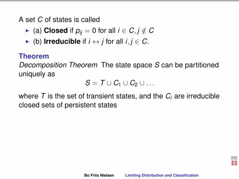
A set C of states is called
I (a) Closed if pij = 0 for all i ∈ C, j /∈ CI (b) Irreducible if i ↔ j for all i , j ∈ C.
TheoremDecomposition Theorem The state space S can be partitioneduniquely as
S = T ∪ C1 ∪ C2 ∪ . . .
where T is the set of transient states, and the Ci are irreducibleclosed sets of persistent states �
LemmaIf S is finite, then at least one state is persistent(recurrent) andall persistent states are non-null (positive recurrent) �
Bo Friis Nielsen Limiting Distribution and Classification

A set C of states is calledI (a) Closed if pij = 0 for all i ∈ C, j /∈ C
I (b) Irreducible if i ↔ j for all i , j ∈ C.
TheoremDecomposition Theorem The state space S can be partitioneduniquely as
S = T ∪ C1 ∪ C2 ∪ . . .
where T is the set of transient states, and the Ci are irreducibleclosed sets of persistent states �
LemmaIf S is finite, then at least one state is persistent(recurrent) andall persistent states are non-null (positive recurrent) �
Bo Friis Nielsen Limiting Distribution and Classification

A set C of states is calledI (a) Closed if pij = 0 for all i ∈ C, j /∈ CI (b) Irreducible if i ↔ j for all i , j ∈ C.
Theorem
Decomposition Theorem The state space S can be partitioneduniquely as
S = T ∪ C1 ∪ C2 ∪ . . .
where T is the set of transient states, and the Ci are irreducibleclosed sets of persistent states �
LemmaIf S is finite, then at least one state is persistent(recurrent) andall persistent states are non-null (positive recurrent) �
Bo Friis Nielsen Limiting Distribution and Classification

A set C of states is calledI (a) Closed if pij = 0 for all i ∈ C, j /∈ CI (b) Irreducible if i ↔ j for all i , j ∈ C.
TheoremDecomposition Theorem The state space S can be partitioneduniquely as
S = T ∪ C1 ∪ C2 ∪ . . .
where T is the set of transient states, and the Ci are irreducibleclosed sets of persistent states �
LemmaIf S is finite, then at least one state is persistent(recurrent) andall persistent states are non-null (positive recurrent) �
Bo Friis Nielsen Limiting Distribution and Classification
A set C of states is calledI (a) Closed if pij = 0 for all i ∈ C, j /∈ CI (b) Irreducible if i ↔ j for all i , j ∈ C.
TheoremDecomposition Theorem The state space S can be partitioneduniquely as
S = T ∪ C1 ∪ C2 ∪ . . .
where T is the set of transient states, and the Ci are irreducibleclosed sets of persistent states
�
LemmaIf S is finite, then at least one state is persistent(recurrent) andall persistent states are non-null (positive recurrent) �
Bo Friis Nielsen Limiting Distribution and Classification

A set C of states is calledI (a) Closed if pij = 0 for all i ∈ C, j /∈ CI (b) Irreducible if i ↔ j for all i , j ∈ C.
TheoremDecomposition Theorem The state space S can be partitioneduniquely as
S = T ∪ C1 ∪ C2 ∪ . . .
where T is the set of transient states, and the Ci are irreducibleclosed sets of persistent states �
LemmaIf S is finite, then at least one state is persistent(recurrent) andall persistent states are non-null (positive recurrent) �
Bo Friis Nielsen Limiting Distribution and Classification

Basic Limit Theorem
Theorem 4.3 The basic limit theorem of Markov chains
(a) Consider a recurrent irreducible aperiodic Markovchain. Let P(n)
ii be the probability of entering state iat the nth transition, n = 1,2, . . . , given thatX0 = i . By our earlier convention P(0)
ii = 1. Let f (n)iibe the probability of first returning to state i at thenth transition n = 1,2, . . . , where f (0)ii = 0. Then
limn→∞
P(n)ii =
1∑∞n=0 nf (n)ii
=1mi
(b) under the same conditions as in (a),limn→∞ P(n)
ji = limn→∞ P(n)ii for all j .
Bo Friis Nielsen Limiting Distribution and Classification

An example chain (random walk with reflectingbarriers)
P
=
0.6 0.4 0.0 0.0 0.0 0.0 0.0 0.00.3 0.3 0.4 0.0 0.0 0.0 0.0 0.00.0 0.3 0.3 0.4 0.0 0.0 0.0 0.00.0 0.0 0.3 0.3 0.4 0.0 0.0 0.00.0 0.0 0.0 0.3 0.3 0.4 0.0 0.00.0 0.0 0.0 0.0 0.3 0.3 0.4 0.00.0 0.0 0.0 0.0 0.0 0.3 0.3 0.40.0 0.0 0.0 0.0 0.0 0.0 0.3 0.7
With initial probability distribution p(0) = (1,0,0,0,0,0,0,0) or
X0 = 1.
Bo Friis Nielsen Limiting Distribution and Classification

An example chain (random walk with reflectingbarriers)
P =
0.6 0.4 0.0 0.0 0.0 0.0 0.0 0.00.3 0.3 0.4 0.0 0.0 0.0 0.0 0.00.0 0.3 0.3 0.4 0.0 0.0 0.0 0.00.0 0.0 0.3 0.3 0.4 0.0 0.0 0.00.0 0.0 0.0 0.3 0.3 0.4 0.0 0.00.0 0.0 0.0 0.0 0.3 0.3 0.4 0.00.0 0.0 0.0 0.0 0.0 0.3 0.3 0.40.0 0.0 0.0 0.0 0.0 0.0 0.3 0.7
With initial probability distribution p(0) = (1,0,0,0,0,0,0,0) orX0 = 1.
Bo Friis Nielsen Limiting Distribution and Classification

An example chain (random walk with reflectingbarriers)
P =
0.6 0.4 0.0 0.0 0.0 0.0 0.0 0.00.3 0.3 0.4 0.0 0.0 0.0 0.0 0.00.0 0.3 0.3 0.4 0.0 0.0 0.0 0.00.0 0.0 0.3 0.3 0.4 0.0 0.0 0.00.0 0.0 0.0 0.3 0.3 0.4 0.0 0.00.0 0.0 0.0 0.0 0.3 0.3 0.4 0.00.0 0.0 0.0 0.0 0.0 0.3 0.3 0.40.0 0.0 0.0 0.0 0.0 0.0 0.3 0.7
With initial probability distribution p(0) = (1,0,0,0,0,0,0,0) or
X0 = 1.
Bo Friis Nielsen Limiting Distribution and Classification

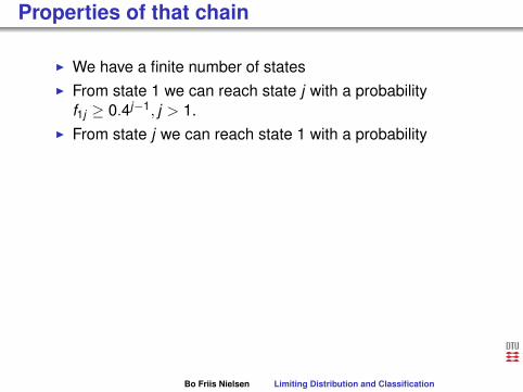
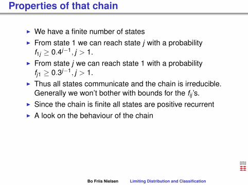
Properties of that chain
I We have a finite number of statesI From state 1 we can reach state j with a probability
f1j ≥ 0.4j−1, j > 1.I From state j we can reach state 1 with a probability
fj1 ≥ 0.3j−1, j > 1.I Thus all states communicate and the chain is irreducible.
Generally we won’t bother with bounds for the fij ’s.I Since the chain is finite all states are positive recurrentI A look on the behaviour of the chain
Bo Friis Nielsen Limiting Distribution and Classification

Properties of that chain
I We have a finite number of states
I From state 1 we can reach state j with a probabilityf1j ≥ 0.4j−1, j > 1.
I From state j we can reach state 1 with a probabilityfj1 ≥ 0.3j−1, j > 1.
I Thus all states communicate and the chain is irreducible.Generally we won’t bother with bounds for the fij ’s.
I Since the chain is finite all states are positive recurrentI A look on the behaviour of the chain
Bo Friis Nielsen Limiting Distribution and Classification

Properties of that chain
I We have a finite number of statesI From state 1 we can reach state j
with a probabilityf1j ≥ 0.4j−1, j > 1.
I From state j we can reach state 1 with a probabilityfj1 ≥ 0.3j−1, j > 1.
I Thus all states communicate and the chain is irreducible.Generally we won’t bother with bounds for the fij ’s.
I Since the chain is finite all states are positive recurrentI A look on the behaviour of the chain
Bo Friis Nielsen Limiting Distribution and Classification

Properties of that chain
I We have a finite number of statesI From state 1 we can reach state j with a probability
f1j ≥ 0.4j−1, j > 1.I From state j we can reach state 1 with a probability
fj1 ≥ 0.3j−1, j > 1.I Thus all states communicate and the chain is irreducible.
Generally we won’t bother with bounds for the fij ’s.I Since the chain is finite all states are positive recurrentI A look on the behaviour of the chain
Bo Friis Nielsen Limiting Distribution and Classification

Properties of that chain
I We have a finite number of statesI From state 1 we can reach state j with a probability
f1j ≥ 0.4j−1,
j > 1.I From state j we can reach state 1 with a probability
fj1 ≥ 0.3j−1, j > 1.I Thus all states communicate and the chain is irreducible.
Generally we won’t bother with bounds for the fij ’s.I Since the chain is finite all states are positive recurrentI A look on the behaviour of the chain
Bo Friis Nielsen Limiting Distribution and Classification

Properties of that chain
I We have a finite number of statesI From state 1 we can reach state j with a probability
f1j ≥ 0.4j−1, j > 1.
I From state j we can reach state 1 with a probabilityfj1 ≥ 0.3j−1, j > 1.
I Thus all states communicate and the chain is irreducible.Generally we won’t bother with bounds for the fij ’s.
I Since the chain is finite all states are positive recurrentI A look on the behaviour of the chain
Bo Friis Nielsen Limiting Distribution and Classification
Properties of that chain
I We have a finite number of statesI From state 1 we can reach state j with a probability
f1j ≥ 0.4j−1, j > 1.I From state j we can reach state 1 with a probability
fj1 ≥ 0.3j−1, j > 1.I Thus all states communicate and the chain is irreducible.
Generally we won’t bother with bounds for the fij ’s.I Since the chain is finite all states are positive recurrentI A look on the behaviour of the chain
Bo Friis Nielsen Limiting Distribution and Classification

Properties of that chain
I We have a finite number of statesI From state 1 we can reach state j with a probability
f1j ≥ 0.4j−1, j > 1.I From state j we can reach state 1 with a probability
fj1 ≥ 0.3j−1,
j > 1.I Thus all states communicate and the chain is irreducible.
Generally we won’t bother with bounds for the fij ’s.I Since the chain is finite all states are positive recurrentI A look on the behaviour of the chain
Bo Friis Nielsen Limiting Distribution and Classification

Properties of that chain
I We have a finite number of statesI From state 1 we can reach state j with a probability
f1j ≥ 0.4j−1, j > 1.I From state j we can reach state 1 with a probability
fj1 ≥ 0.3j−1, j > 1.
I Thus all states communicate and the chain is irreducible.Generally we won’t bother with bounds for the fij ’s.
I Since the chain is finite all states are positive recurrentI A look on the behaviour of the chain
Bo Friis Nielsen Limiting Distribution and Classification

Properties of that chain
I We have a finite number of statesI From state 1 we can reach state j with a probability
f1j ≥ 0.4j−1, j > 1.I From state j we can reach state 1 with a probability
fj1 ≥ 0.3j−1, j > 1.I Thus all states communicate and the chain is irreducible.
Generally we won’t bother with bounds for the fij ’s.I Since the chain is finite all states are positive recurrentI A look on the behaviour of the chain
Bo Friis Nielsen Limiting Distribution and Classification

Properties of that chain
I We have a finite number of statesI From state 1 we can reach state j with a probability
f1j ≥ 0.4j−1, j > 1.I From state j we can reach state 1 with a probability
fj1 ≥ 0.3j−1, j > 1.I Thus all states communicate and the chain is irreducible.
Generally we won’t bother with bounds for the fij ’s.
I Since the chain is finite all states are positive recurrentI A look on the behaviour of the chain
Bo Friis Nielsen Limiting Distribution and Classification

Properties of that chain
I We have a finite number of statesI From state 1 we can reach state j with a probability
f1j ≥ 0.4j−1, j > 1.I From state j we can reach state 1 with a probability
fj1 ≥ 0.3j−1, j > 1.I Thus all states communicate and the chain is irreducible.
Generally we won’t bother with bounds for the fij ’s.I Since the chain is finite all states are positive recurrent
I A look on the behaviour of the chain
Bo Friis Nielsen Limiting Distribution and Classification
Properties of that chain
I We have a finite number of statesI From state 1 we can reach state j with a probability
f1j ≥ 0.4j−1, j > 1.I From state j we can reach state 1 with a probability
fj1 ≥ 0.3j−1, j > 1.I Thus all states communicate and the chain is irreducible.
Generally we won’t bother with bounds for the fij ’s.I Since the chain is finite all states are positive recurrentI A look on the behaviour of the chain
Bo Friis Nielsen Limiting Distribution and Classification

A number of different sample paths Xn’s
0 10 20 30 40 50 60 701
2
3
4
5
6
7
8
0 10 20 30 40 50 60 701
2
3
4
5
6
7
8
0 10 20 30 40 50 60 701
2
3
4
5
6
7
8
0 10 20 30 40 50 60 701
2
3
4
5
6
7
8
Bo Friis Nielsen Limiting Distribution and Classification

A number of different sample paths Xn’s
0 10 20 30 40 50 60 701
2
3
4
5
6
7
8
0 10 20 30 40 50 60 701
2
3
4
5
6
7
8
0 10 20 30 40 50 60 701
2
3
4
5
6
7
8
0 10 20 30 40 50 60 701
2
3
4
5
6
7
8
Bo Friis Nielsen Limiting Distribution and Classification

A number of different sample paths Xn’s
0 10 20 30 40 50 60 701
2
3
4
5
6
7
8
0 10 20 30 40 50 60 701
2
3
4
5
6
7
8
0 10 20 30 40 50 60 701
2
3
4
5
6
7
8
0 10 20 30 40 50 60 701
2
3
4
5
6
7
8
Bo Friis Nielsen Limiting Distribution and Classification

A number of different sample paths Xn’s
0 10 20 30 40 50 60 701
2
3
4
5
6
7
8
0 10 20 30 40 50 60 701
2
3
4
5
6
7
8
0 10 20 30 40 50 60 701
2
3
4
5
6
7
8
0 10 20 30 40 50 60 701
2
3
4
5
6
7
8
Bo Friis Nielsen Limiting Distribution and Classification

A number of different sample paths Xn’s
0 10 20 30 40 50 60 701
2
3
4
5
6
7
8
0 10 20 30 40 50 60 701
2
3
4
5
6
7
8
0 10 20 30 40 50 60 701
2
3
4
5
6
7
8
0 10 20 30 40 50 60 701
2
3
4
5
6
7
8
Bo Friis Nielsen Limiting Distribution and Classification

The state probabilities
p(n)j
0 10 20 30 40 50 60 700
0.1
0.2
0.3
0.4
0.5
0.6
0.7
0.8
0.9
1
Bo Friis Nielsen Limiting Distribution and Classification

The state probabilities
p(n)j
0 10 20 30 40 50 60 700
0.1
0.2
0.3
0.4
0.5
0.6
0.7
0.8
0.9
1
Bo Friis Nielsen Limiting Distribution and Classification

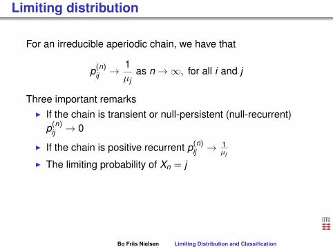
Limiting distribution
For an irreducible aperiodic chain, we have that
p(n)ij
→ 1µj
as n→∞, for all i and j
Three important remarksI If the chain is transient or null-persistent (null-recurrent)
p(n)ij → 0
I If the chain is positive recurrent p(n)ij →
1µj
I The limiting probability of Xn = j does not depend on thestarting state X0 = i
Bo Friis Nielsen Limiting Distribution and Classification

Limiting distribution
For an irreducible aperiodic chain, we have that
p(n)ij →
1µj
as n→∞, for all i and j
Three important remarks
I If the chain is transient or null-persistent (null-recurrent)p(n)
ij → 0
I If the chain is positive recurrent p(n)ij →
1µj
I The limiting probability of Xn = j does not depend on thestarting state X0 = i
Bo Friis Nielsen Limiting Distribution and Classification

Limiting distribution
For an irreducible aperiodic chain, we have that
p(n)ij →
1µj
as n→∞, for all i and j
Three important remarksI If the chain is transient or null-persistent (null-recurrent)
p(n)ij → 0
I If the chain is positive recurrent p(n)ij →
1µj
I The limiting probability of Xn = j does not depend on thestarting state X0 = i
Bo Friis Nielsen Limiting Distribution and Classification

Limiting distribution
For an irreducible aperiodic chain, we have that
p(n)ij →
1µj
as n→∞, for all i and j
Three important remarksI If the chain is transient or null-persistent (null-recurrent)
p(n)ij → 0
I If the chain is positive recurrent p(n)ij →
1µj
I The limiting probability of Xn = j does not depend on thestarting state X0 = i
Bo Friis Nielsen Limiting Distribution and Classification
Limiting distribution
For an irreducible aperiodic chain, we have that
p(n)ij →
1µj
as n→∞, for all i and j
Three important remarksI If the chain is transient or null-persistent (null-recurrent)
p(n)ij → 0
I If the chain is positive recurrent p(n)ij →
1µj
I The limiting probability of Xn = j
does not depend on thestarting state X0 = i
Bo Friis Nielsen Limiting Distribution and Classification

Limiting distribution
For an irreducible aperiodic chain, we have that
p(n)ij →
1µj
as n→∞, for all i and j
Three important remarksI If the chain is transient or null-persistent (null-recurrent)
p(n)ij → 0
I If the chain is positive recurrent p(n)ij →
1µj
I The limiting probability of Xn = j does not depend on thestarting state X0 = i
Bo Friis Nielsen Limiting Distribution and Classification

The stationary distribution
I A distribution that does not change with n
I The elements of p(n) are all constantI The implication of this is p(n) = p(n−1)P = p(n−1) by our
assumption of p(n) being constantI Expressed differently π = πP
Bo Friis Nielsen Limiting Distribution and Classification

The stationary distribution
I A distribution that does not change with nI The elements of p(n) are all constant
I The implication of this is p(n) = p(n−1)P = p(n−1) by ourassumption of p(n) being constant
I Expressed differently π = πP
Bo Friis Nielsen Limiting Distribution and Classification
The stationary distribution
I A distribution that does not change with nI The elements of p(n) are all constantI The implication of this is p(n)
= p(n−1)P = p(n−1) by ourassumption of p(n) being constant
I Expressed differently π = πP
Bo Friis Nielsen Limiting Distribution and Classification

The stationary distribution
I A distribution that does not change with nI The elements of p(n) are all constantI The implication of this is p(n) = p(n−1)P
= p(n−1) by ourassumption of p(n) being constant
I Expressed differently π = πP
Bo Friis Nielsen Limiting Distribution and Classification
The stationary distribution
I A distribution that does not change with nI The elements of p(n) are all constantI The implication of this is p(n) = p(n−1)P = p(n−1)
by ourassumption of p(n) being constant
I Expressed differently π = πP
Bo Friis Nielsen Limiting Distribution and Classification

The stationary distribution
I A distribution that does not change with nI The elements of p(n) are all constantI The implication of this is p(n) = p(n−1)P = p(n−1) by our
assumption of p(n) being constant
I Expressed differently π = πP
Bo Friis Nielsen Limiting Distribution and Classification
The stationary distribution
I A distribution that does not change with nI The elements of p(n) are all constantI The implication of this is p(n) = p(n−1)P = p(n−1) by our
assumption of p(n) being constantI Expressed differently
π = πP
Bo Friis Nielsen Limiting Distribution and Classification

The stationary distribution
I A distribution that does not change with nI The elements of p(n) are all constantI The implication of this is p(n) = p(n−1)P = p(n−1) by our
assumption of p(n) being constantI Expressed differently π =
πP
Bo Friis Nielsen Limiting Distribution and Classification

The stationary distribution
I A distribution that does not change with nI The elements of p(n) are all constantI The implication of this is p(n) = p(n−1)P = p(n−1) by our
assumption of p(n) being constantI Expressed differently π = π
P
Bo Friis Nielsen Limiting Distribution and Classification

The stationary distribution
I A distribution that does not change with nI The elements of p(n) are all constantI The implication of this is p(n) = p(n−1)P = p(n−1) by our
assumption of p(n) being constantI Expressed differently π = πP
Bo Friis Nielsen Limiting Distribution and Classification

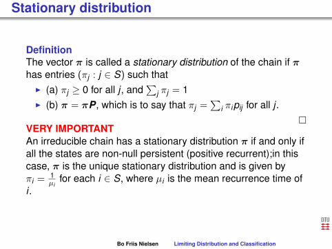
Stationary distribution
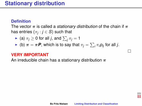
DefinitionThe vector π is called a stationary distribution of the chain if πhas entries (πj : j ∈ S) such that
I (a) πj ≥ 0 for all j , and∑
j πj = 1I (b) π = πP, which is to say that πj =
∑i πipij for all j .
�VERY IMPORTANTAn irreducible chain has a stationary distribution π if and only ifall the states are non-null persistent (positive recurrent);in thiscase, π is the unique stationary distribution and is given byπi =
1µi
for each i ∈ S, where µi is the mean recurrence time ofi .
Bo Friis Nielsen Limiting Distribution and Classification

Stationary distribution
DefinitionThe vector π is called a stationary distribution of the chain if πhas entries (πj : j ∈ S) such thatI (a) πj ≥ 0 for all j , and
∑j πj = 1
I (b) π = πP, which is to say that πj =∑
i πipij for all j .�
VERY IMPORTANTAn irreducible chain has a stationary distribution π if and only ifall the states are non-null persistent (positive recurrent);in thiscase, π is the unique stationary distribution and is given byπi =
1µi
for each i ∈ S, where µi is the mean recurrence time ofi .
Bo Friis Nielsen Limiting Distribution and Classification

Stationary distribution
DefinitionThe vector π is called a stationary distribution of the chain if πhas entries (πj : j ∈ S) such thatI (a) πj ≥ 0 for all j , and
∑j πj = 1
I (b) π = πP, which is to say that πj =∑
i πipij for all j .�
VERY IMPORTANT
An irreducible chain has a stationary distribution π if and only ifall the states are non-null persistent (positive recurrent);in thiscase, π is the unique stationary distribution and is given byπi =
1µi
for each i ∈ S, where µi is the mean recurrence time ofi .
Bo Friis Nielsen Limiting Distribution and Classification
Stationary distribution
DefinitionThe vector π is called a stationary distribution of the chain if πhas entries (πj : j ∈ S) such thatI (a) πj ≥ 0 for all j , and
∑j πj = 1
I (b) π = πP, which is to say that πj =∑
i πipij for all j .�
VERY IMPORTANTAn irreducible chain has a stationary distribution π
if and only ifall the states are non-null persistent (positive recurrent);in thiscase, π is the unique stationary distribution and is given byπi =
1µi
for each i ∈ S, where µi is the mean recurrence time ofi .
Bo Friis Nielsen Limiting Distribution and Classification

Stationary distribution
DefinitionThe vector π is called a stationary distribution of the chain if πhas entries (πj : j ∈ S) such thatI (a) πj ≥ 0 for all j , and
∑j πj = 1
I (b) π = πP, which is to say that πj =∑
i πipij for all j .�
VERY IMPORTANTAn irreducible chain has a stationary distribution π if and only ifall the states are non-null persistent
(positive recurrent);in thiscase, π is the unique stationary distribution and is given byπi =
1µi
for each i ∈ S, where µi is the mean recurrence time ofi .
Bo Friis Nielsen Limiting Distribution and Classification

Stationary distribution
DefinitionThe vector π is called a stationary distribution of the chain if πhas entries (πj : j ∈ S) such thatI (a) πj ≥ 0 for all j , and
∑j πj = 1
I (b) π = πP, which is to say that πj =∑
i πipij for all j .�
VERY IMPORTANTAn irreducible chain has a stationary distribution π if and only ifall the states are non-null persistent (positive recurrent);
in thiscase, π is the unique stationary distribution and is given byπi =
1µi
for each i ∈ S, where µi is the mean recurrence time ofi .
Bo Friis Nielsen Limiting Distribution and Classification

Stationary distribution
DefinitionThe vector π is called a stationary distribution of the chain if πhas entries (πj : j ∈ S) such thatI (a) πj ≥ 0 for all j , and
∑j πj = 1
I (b) π = πP, which is to say that πj =∑
i πipij for all j .�
VERY IMPORTANTAn irreducible chain has a stationary distribution π if and only ifall the states are non-null persistent (positive recurrent);in thiscase, π is the unique stationary distribution
and is given byπi =
1µi
for each i ∈ S, where µi is the mean recurrence time ofi .
Bo Friis Nielsen Limiting Distribution and Classification

Stationary distribution
DefinitionThe vector π is called a stationary distribution of the chain if πhas entries (πj : j ∈ S) such thatI (a) πj ≥ 0 for all j , and
∑j πj = 1
I (b) π = πP, which is to say that πj =∑
i πipij for all j .�
VERY IMPORTANTAn irreducible chain has a stationary distribution π if and only ifall the states are non-null persistent (positive recurrent);in thiscase, π is the unique stationary distribution and is given byπi =
1µi
for each i ∈ S,
where µi is the mean recurrence time ofi .
Bo Friis Nielsen Limiting Distribution and Classification
Stationary distribution
DefinitionThe vector π is called a stationary distribution of the chain if πhas entries (πj : j ∈ S) such thatI (a) πj ≥ 0 for all j , and
∑j πj = 1
I (b) π = πP, which is to say that πj =∑
i πipij for all j .�
VERY IMPORTANTAn irreducible chain has a stationary distribution π if and only ifall the states are non-null persistent (positive recurrent);in thiscase, π is the unique stationary distribution and is given byπi =
1µi
for each i ∈ S, where µi is the mean recurrence time ofi .
Bo Friis Nielsen Limiting Distribution and Classification

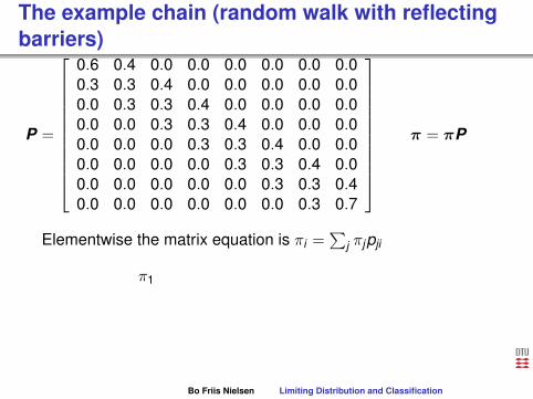
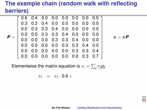
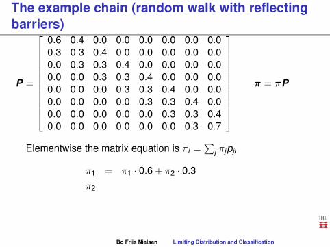
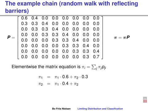
The example chain (random walk with reflectingbarriers)
P =
0.6 0.4 0.0 0.0 0.0 0.0 0.0 0.00.3 0.3 0.4 0.0 0.0 0.0 0.0 0.00.0 0.3 0.3 0.4 0.0 0.0 0.0 0.00.0 0.0 0.3 0.3 0.4 0.0 0.0 0.00.0 0.0 0.0 0.3 0.3 0.4 0.0 0.00.0 0.0 0.0 0.0 0.3 0.3 0.4 0.00.0 0.0 0.0 0.0 0.0 0.3 0.3 0.40.0 0.0 0.0 0.0 0.0 0.0 0.3 0.7
π = πP
Elementwise the matrix equation is πi =∑
j πjpji
π1 = π1 · 0.6 + π2 · 0.3π2 = π1 · 0.4 + π2 · 0.3 + π3 · 0.3π3 = π2 · 0.4 + π3 · 0.3 + π4 · 0.3
Bo Friis Nielsen Limiting Distribution and Classification
The example chain (random walk with reflectingbarriers)
P =
0.6 0.4 0.0 0.0 0.0 0.0 0.0 0.00.3 0.3 0.4 0.0 0.0 0.0 0.0 0.00.0 0.3 0.3 0.4 0.0 0.0 0.0 0.00.0 0.0 0.3 0.3 0.4 0.0 0.0 0.00.0 0.0 0.0 0.3 0.3 0.4 0.0 0.00.0 0.0 0.0 0.0 0.3 0.3 0.4 0.00.0 0.0 0.0 0.0 0.0 0.3 0.3 0.40.0 0.0 0.0 0.0 0.0 0.0 0.3 0.7
π = πP
Elementwise the matrix equation is πi =∑
j πjpji
π1
= π1 · 0.6 + π2 · 0.3π2 = π1 · 0.4 + π2 · 0.3 + π3 · 0.3π3 = π2 · 0.4 + π3 · 0.3 + π4 · 0.3
Bo Friis Nielsen Limiting Distribution and Classification

The example chain (random walk with reflectingbarriers)
P =
0.6 0.4 0.0 0.0 0.0 0.0 0.0 0.00.3 0.3 0.4 0.0 0.0 0.0 0.0 0.00.0 0.3 0.3 0.4 0.0 0.0 0.0 0.00.0 0.0 0.3 0.3 0.4 0.0 0.0 0.00.0 0.0 0.0 0.3 0.3 0.4 0.0 0.00.0 0.0 0.0 0.0 0.3 0.3 0.4 0.00.0 0.0 0.0 0.0 0.0 0.3 0.3 0.40.0 0.0 0.0 0.0 0.0 0.0 0.3 0.7
π = πP
Elementwise the matrix equation is πi =∑
j πjpji
π1 = π1
· 0.6 + π2 · 0.3π2 = π1 · 0.4 + π2 · 0.3 + π3 · 0.3π3 = π2 · 0.4 + π3 · 0.3 + π4 · 0.3
Bo Friis Nielsen Limiting Distribution and Classification
The example chain (random walk with reflectingbarriers)
P =
0.6 0.4 0.0 0.0 0.0 0.0 0.0 0.00.3 0.3 0.4 0.0 0.0 0.0 0.0 0.00.0 0.3 0.3 0.4 0.0 0.0 0.0 0.00.0 0.0 0.3 0.3 0.4 0.0 0.0 0.00.0 0.0 0.0 0.3 0.3 0.4 0.0 0.00.0 0.0 0.0 0.0 0.3 0.3 0.4 0.00.0 0.0 0.0 0.0 0.0 0.3 0.3 0.40.0 0.0 0.0 0.0 0.0 0.0 0.3 0.7
π = πP
Elementwise the matrix equation is πi =∑
j πjpji
π1 = π1 · 0.6 +
π2 · 0.3π2 = π1 · 0.4 + π2 · 0.3 + π3 · 0.3π3 = π2 · 0.4 + π3 · 0.3 + π4 · 0.3
Bo Friis Nielsen Limiting Distribution and Classification

The example chain (random walk with reflectingbarriers)
P =
0.6 0.4 0.0 0.0 0.0 0.0 0.0 0.00.3 0.3 0.4 0.0 0.0 0.0 0.0 0.00.0 0.3 0.3 0.4 0.0 0.0 0.0 0.00.0 0.0 0.3 0.3 0.4 0.0 0.0 0.00.0 0.0 0.0 0.3 0.3 0.4 0.0 0.00.0 0.0 0.0 0.0 0.3 0.3 0.4 0.00.0 0.0 0.0 0.0 0.0 0.3 0.3 0.40.0 0.0 0.0 0.0 0.0 0.0 0.3 0.7
π = πP
Elementwise the matrix equation is πi =∑
j πjpji
π1 = π1 · 0.6 + π2
· 0.3π2 = π1 · 0.4 + π2 · 0.3 + π3 · 0.3π3 = π2 · 0.4 + π3 · 0.3 + π4 · 0.3
Bo Friis Nielsen Limiting Distribution and Classification

The example chain (random walk with reflectingbarriers)
P =
0.6 0.4 0.0 0.0 0.0 0.0 0.0 0.00.3 0.3 0.4 0.0 0.0 0.0 0.0 0.00.0 0.3 0.3 0.4 0.0 0.0 0.0 0.00.0 0.0 0.3 0.3 0.4 0.0 0.0 0.00.0 0.0 0.0 0.3 0.3 0.4 0.0 0.00.0 0.0 0.0 0.0 0.3 0.3 0.4 0.00.0 0.0 0.0 0.0 0.0 0.3 0.3 0.40.0 0.0 0.0 0.0 0.0 0.0 0.3 0.7
π = πP
Elementwise the matrix equation is πi =∑
j πjpji
π1 = π1 · 0.6 + π2 · 0.3
π2 = π1 · 0.4 + π2 · 0.3 + π3 · 0.3π3 = π2 · 0.4 + π3 · 0.3 + π4 · 0.3
Bo Friis Nielsen Limiting Distribution and Classification
The example chain (random walk with reflectingbarriers)
P =
0.6 0.4 0.0 0.0 0.0 0.0 0.0 0.00.3 0.3 0.4 0.0 0.0 0.0 0.0 0.00.0 0.3 0.3 0.4 0.0 0.0 0.0 0.00.0 0.0 0.3 0.3 0.4 0.0 0.0 0.00.0 0.0 0.0 0.3 0.3 0.4 0.0 0.00.0 0.0 0.0 0.0 0.3 0.3 0.4 0.00.0 0.0 0.0 0.0 0.0 0.3 0.3 0.40.0 0.0 0.0 0.0 0.0 0.0 0.3 0.7
π = πP
Elementwise the matrix equation is πi =∑
j πjpji
π1 = π1 · 0.6 + π2 · 0.3π2
= π1 · 0.4 + π2 · 0.3 + π3 · 0.3π3 = π2 · 0.4 + π3 · 0.3 + π4 · 0.3
Bo Friis Nielsen Limiting Distribution and Classification

The example chain (random walk with reflectingbarriers)
P =
0.6 0.4 0.0 0.0 0.0 0.0 0.0 0.00.3 0.3 0.4 0.0 0.0 0.0 0.0 0.00.0 0.3 0.3 0.4 0.0 0.0 0.0 0.00.0 0.0 0.3 0.3 0.4 0.0 0.0 0.00.0 0.0 0.0 0.3 0.3 0.4 0.0 0.00.0 0.0 0.0 0.0 0.3 0.3 0.4 0.00.0 0.0 0.0 0.0 0.0 0.3 0.3 0.40.0 0.0 0.0 0.0 0.0 0.0 0.3 0.7
π = πP
Elementwise the matrix equation is πi =∑
j πjpji
π1 = π1 · 0.6 + π2 · 0.3π2 = π1
· 0.4 + π2 · 0.3 + π3 · 0.3π3 = π2 · 0.4 + π3 · 0.3 + π4 · 0.3
Bo Friis Nielsen Limiting Distribution and Classification

The example chain (random walk with reflectingbarriers)
P =
0.6 0.4 0.0 0.0 0.0 0.0 0.0 0.00.3 0.3 0.4 0.0 0.0 0.0 0.0 0.00.0 0.3 0.3 0.4 0.0 0.0 0.0 0.00.0 0.0 0.3 0.3 0.4 0.0 0.0 0.00.0 0.0 0.0 0.3 0.3 0.4 0.0 0.00.0 0.0 0.0 0.0 0.3 0.3 0.4 0.00.0 0.0 0.0 0.0 0.0 0.3 0.3 0.40.0 0.0 0.0 0.0 0.0 0.0 0.3 0.7
π = πP
Elementwise the matrix equation is πi =∑
j πjpji
π1 = π1 · 0.6 + π2 · 0.3π2 = π1 · 0.4
+ π2 · 0.3 + π3 · 0.3π3 = π2 · 0.4 + π3 · 0.3 + π4 · 0.3
Bo Friis Nielsen Limiting Distribution and Classification
The example chain (random walk with reflectingbarriers)
P =
0.6 0.4 0.0 0.0 0.0 0.0 0.0 0.00.3 0.3 0.4 0.0 0.0 0.0 0.0 0.00.0 0.3 0.3 0.4 0.0 0.0 0.0 0.00.0 0.0 0.3 0.3 0.4 0.0 0.0 0.00.0 0.0 0.0 0.3 0.3 0.4 0.0 0.00.0 0.0 0.0 0.0 0.3 0.3 0.4 0.00.0 0.0 0.0 0.0 0.0 0.3 0.3 0.40.0 0.0 0.0 0.0 0.0 0.0 0.3 0.7
π = πP
Elementwise the matrix equation is πi =∑
j πjpji
π1 = π1 · 0.6 + π2 · 0.3π2 = π1 · 0.4 + π2
· 0.3 + π3 · 0.3π3 = π2 · 0.4 + π3 · 0.3 + π4 · 0.3
Bo Friis Nielsen Limiting Distribution and Classification

The example chain (random walk with reflectingbarriers)
P =
0.6 0.4 0.0 0.0 0.0 0.0 0.0 0.00.3 0.3 0.4 0.0 0.0 0.0 0.0 0.00.0 0.3 0.3 0.4 0.0 0.0 0.0 0.00.0 0.0 0.3 0.3 0.4 0.0 0.0 0.00.0 0.0 0.0 0.3 0.3 0.4 0.0 0.00.0 0.0 0.0 0.0 0.3 0.3 0.4 0.00.0 0.0 0.0 0.0 0.0 0.3 0.3 0.40.0 0.0 0.0 0.0 0.0 0.0 0.3 0.7
π = πP
Elementwise the matrix equation is πi =∑
j πjpji
π1 = π1 · 0.6 + π2 · 0.3π2 = π1 · 0.4 + π2 ·
0.3 + π3 · 0.3π3 = π2 · 0.4 + π3 · 0.3 + π4 · 0.3
Bo Friis Nielsen Limiting Distribution and Classification

The example chain (random walk with reflectingbarriers)
P =
0.6 0.4 0.0 0.0 0.0 0.0 0.0 0.00.3 0.3 0.4 0.0 0.0 0.0 0.0 0.00.0 0.3 0.3 0.4 0.0 0.0 0.0 0.00.0 0.0 0.3 0.3 0.4 0.0 0.0 0.00.0 0.0 0.0 0.3 0.3 0.4 0.0 0.00.0 0.0 0.0 0.0 0.3 0.3 0.4 0.00.0 0.0 0.0 0.0 0.0 0.3 0.3 0.40.0 0.0 0.0 0.0 0.0 0.0 0.3 0.7
π = πP
Elementwise the matrix equation is πi =∑
j πjpji
π1 = π1 · 0.6 + π2 · 0.3π2 = π1 · 0.4 + π2 · 0.3 +
π3 · 0.3π3 = π2 · 0.4 + π3 · 0.3 + π4 · 0.3
Bo Friis Nielsen Limiting Distribution and Classification

The example chain (random walk with reflectingbarriers)
P =
0.6 0.4 0.0 0.0 0.0 0.0 0.0 0.00.3 0.3 0.4 0.0 0.0 0.0 0.0 0.00.0 0.3 0.3 0.4 0.0 0.0 0.0 0.00.0 0.0 0.3 0.3 0.4 0.0 0.0 0.00.0 0.0 0.0 0.3 0.3 0.4 0.0 0.00.0 0.0 0.0 0.0 0.3 0.3 0.4 0.00.0 0.0 0.0 0.0 0.0 0.3 0.3 0.40.0 0.0 0.0 0.0 0.0 0.0 0.3 0.7
π = πP
Elementwise the matrix equation is πi =∑
j πjpji
π1 = π1 · 0.6 + π2 · 0.3π2 = π1 · 0.4 + π2 · 0.3 + π3
· 0.3π3 = π2 · 0.4 + π3 · 0.3 + π4 · 0.3
Bo Friis Nielsen Limiting Distribution and Classification

The example chain (random walk with reflectingbarriers)
P =
0.6 0.4 0.0 0.0 0.0 0.0 0.0 0.00.3 0.3 0.4 0.0 0.0 0.0 0.0 0.00.0 0.3 0.3 0.4 0.0 0.0 0.0 0.00.0 0.0 0.3 0.3 0.4 0.0 0.0 0.00.0 0.0 0.0 0.3 0.3 0.4 0.0 0.00.0 0.0 0.0 0.0 0.3 0.3 0.4 0.00.0 0.0 0.0 0.0 0.0 0.3 0.3 0.40.0 0.0 0.0 0.0 0.0 0.0 0.3 0.7
π = πP
Elementwise the matrix equation is πi =∑
j πjpji
π1 = π1 · 0.6 + π2 · 0.3π2 = π1 · 0.4 + π2 · 0.3 + π3 · 0.3
π3 = π2 · 0.4 + π3 · 0.3 + π4 · 0.3
Bo Friis Nielsen Limiting Distribution and Classification

The example chain (random walk with reflectingbarriers)
P =
0.6 0.4 0.0 0.0 0.0 0.0 0.0 0.00.3 0.3 0.4 0.0 0.0 0.0 0.0 0.00.0 0.3 0.3 0.4 0.0 0.0 0.0 0.00.0 0.0 0.3 0.3 0.4 0.0 0.0 0.00.0 0.0 0.0 0.3 0.3 0.4 0.0 0.00.0 0.0 0.0 0.0 0.3 0.3 0.4 0.00.0 0.0 0.0 0.0 0.0 0.3 0.3 0.40.0 0.0 0.0 0.0 0.0 0.0 0.3 0.7
π = πP
Elementwise the matrix equation is πi =∑
j πjpji
π1 = π1 · 0.6 + π2 · 0.3π2 = π1 · 0.4 + π2 · 0.3 + π3 · 0.3π3 = π2 · 0.4 + π3 · 0.3 + π4 · 0.3
Bo Friis Nielsen Limiting Distribution and Classification

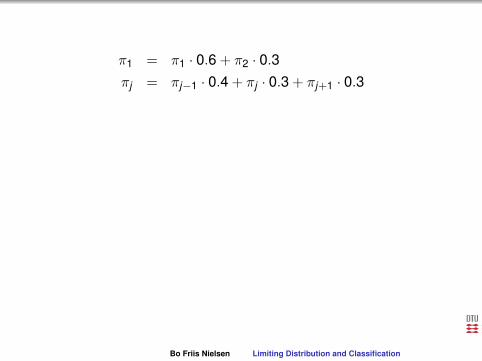
π1 = π1 · 0.6 + π2 · 0.3
πj = πj−1 · 0.4 + πj · 0.3 + πj+1 · 0.3π8 = π7 · 0.4 + π8 · 0.7
Or
π2 =1− 0.6
0.3π1
πj+1 =1
0.3((1− 0.3)πj − 0.4πj−1)
Can be solved recursively to find:
πj =
(0.40.3
)j−1
π1
Bo Friis Nielsen Limiting Distribution and Classification
π1 = π1 · 0.6 + π2 · 0.3πj = πj−1 · 0.4 + πj · 0.3 + πj+1 · 0.3
π8 = π7 · 0.4 + π8 · 0.7
Or
π2 =1− 0.6
0.3π1
πj+1 =1
0.3((1− 0.3)πj − 0.4πj−1)
Can be solved recursively to find:
πj =
(0.40.3
)j−1
π1
Bo Friis Nielsen Limiting Distribution and Classification

π1 = π1 · 0.6 + π2 · 0.3πj = πj−1 · 0.4 + πj · 0.3 + πj+1 · 0.3π8 = π7 · 0.4 + π8 · 0.7
Or
π2 =1− 0.6
0.3π1
πj+1 =1
0.3((1− 0.3)πj − 0.4πj−1)
Can be solved recursively to find:
πj =
(0.40.3
)j−1
π1
Bo Friis Nielsen Limiting Distribution and Classification

π1 = π1 · 0.6 + π2 · 0.3πj = πj−1 · 0.4 + πj · 0.3 + πj+1 · 0.3π8 = π7 · 0.4 + π8 · 0.7
Or
π2 =1− 0.6
0.3π1
πj+1 =1
0.3((1− 0.3)πj − 0.4πj−1)
Can be solved recursively to find:
πj =
(0.40.3
)j−1
π1
Bo Friis Nielsen Limiting Distribution and Classification

π1 = π1 · 0.6 + π2 · 0.3πj = πj−1 · 0.4 + πj · 0.3 + πj+1 · 0.3π8 = π7 · 0.4 + π8 · 0.7
Or
π2 =1− 0.6
0.3π1
πj+1 =1
0.3((1− 0.3)πj − 0.4πj−1)
Can be solved recursively to find:
πj =
(0.40.3
)j−1
π1
Bo Friis Nielsen Limiting Distribution and Classification

π1 = π1 · 0.6 + π2 · 0.3πj = πj−1 · 0.4 + πj · 0.3 + πj+1 · 0.3π8 = π7 · 0.4 + π8 · 0.7
Or
π2 =1− 0.6
0.3π1
πj+1 =1
0.3((1− 0.3)πj − 0.4πj−1)
Can be solved recursively
to find:
πj =
(0.40.3
)j−1
π1
Bo Friis Nielsen Limiting Distribution and Classification

π1 = π1 · 0.6 + π2 · 0.3πj = πj−1 · 0.4 + πj · 0.3 + πj+1 · 0.3π8 = π7 · 0.4 + π8 · 0.7
Or
π2 =1− 0.6
0.3π1
πj+1 =1
0.3((1− 0.3)πj − 0.4πj−1)
Can be solved recursively to find:
πj =
(0.40.3
)j−1
π1
Bo Friis Nielsen Limiting Distribution and Classification

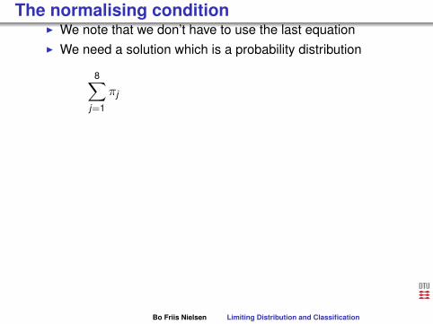
The normalising conditionI We note that we don’t have to use the last equation
I We need a solution which is a probability distribution
8∑j=1
πj = 1,8∑
j=1
(0.40.3
)j−1
π1 = π1
7∑k=0
(0.40.3
)k
N∑i=0
ai =
1−aN+1
1−a N <∞,a 6= 1N + 1 N <∞,a = 1
11−a N =∞, |a| < 1
Such that
1 = π11−
(0.40.3
)8
1− 0.40.3
⇔ π1 =1− 0.4
0.3
1−(0.4
0.3
)8
Bo Friis Nielsen Limiting Distribution and Classification

The normalising conditionI We note that we don’t have to use the last equationI We need a solution which is a probability distribution
8∑j=1
πj = 1,8∑
j=1
(0.40.3
)j−1
π1 = π1
7∑k=0
(0.40.3
)k
N∑i=0
ai =
1−aN+1
1−a N <∞,a 6= 1N + 1 N <∞,a = 1
11−a N =∞, |a| < 1
Such that
1 = π11−
(0.40.3
)8
1− 0.40.3
⇔ π1 =1− 0.4
0.3
1−(0.4
0.3
)8
Bo Friis Nielsen Limiting Distribution and Classification
The normalising conditionI We note that we don’t have to use the last equationI We need a solution which is a probability distribution
8∑j=1
πj
= 1,8∑
j=1
(0.40.3
)j−1
π1 = π1
7∑k=0
(0.40.3
)k
N∑i=0
ai =
1−aN+1
1−a N <∞,a 6= 1N + 1 N <∞,a = 1
11−a N =∞, |a| < 1
Such that
1 = π11−
(0.40.3
)8
1− 0.40.3
⇔ π1 =1− 0.4
0.3
1−(0.4
0.3
)8
Bo Friis Nielsen Limiting Distribution and Classification

The normalising conditionI We note that we don’t have to use the last equationI We need a solution which is a probability distribution
8∑j=1
πj = 1,8∑
j=1
(0.40.3
)j−1
π1 = π1
7∑k=0
(0.40.3
)k
N∑i=0
ai =
1−aN+1
1−a N <∞,a 6= 1N + 1 N <∞,a = 1
11−a N =∞, |a| < 1
Such that
1 = π11−
(0.40.3
)8
1− 0.40.3
⇔ π1 =1− 0.4
0.3
1−(0.4
0.3
)8
Bo Friis Nielsen Limiting Distribution and Classification

The normalising conditionI We note that we don’t have to use the last equationI We need a solution which is a probability distribution
8∑j=1
πj = 1,8∑
j=1
(0.40.3
)j−1
π1
= π1
7∑k=0
(0.40.3
)k
N∑i=0
ai =
1−aN+1
1−a N <∞,a 6= 1N + 1 N <∞,a = 1
11−a N =∞, |a| < 1
Such that
1 = π11−
(0.40.3
)8
1− 0.40.3
⇔ π1 =1− 0.4
0.3
1−(0.4
0.3
)8
Bo Friis Nielsen Limiting Distribution and Classification

The normalising conditionI We note that we don’t have to use the last equationI We need a solution which is a probability distribution
8∑j=1
πj = 1,8∑
j=1
(0.40.3
)j−1
π1 = π1
7∑k=0
(0.40.3
)k
N∑i=0
ai =
1−aN+1
1−a N <∞,a 6= 1N + 1 N <∞,a = 1
11−a N =∞, |a| < 1
Such that
1 = π11−
(0.40.3
)8
1− 0.40.3
⇔ π1 =1− 0.4
0.3
1−(0.4
0.3
)8
Bo Friis Nielsen Limiting Distribution and Classification
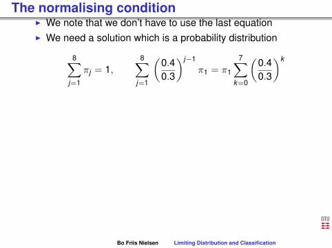
The normalising conditionI We note that we don’t have to use the last equationI We need a solution which is a probability distribution
8∑j=1
πj = 1,8∑
j=1
(0.40.3
)j−1
π1 = π1
7∑k=0
(0.40.3
)k
N∑i=0
ai =
1−aN+1
1−a N <∞,a 6= 1N + 1 N <∞,a = 1
11−a N =∞, |a| < 1
Such that
1 = π11−
(0.40.3
)8
1− 0.40.3
⇔ π1 =1− 0.4
0.3
1−(0.4
0.3
)8
Bo Friis Nielsen Limiting Distribution and Classification
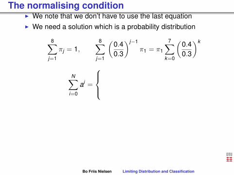
The normalising conditionI We note that we don’t have to use the last equationI We need a solution which is a probability distribution
8∑j=1
πj = 1,8∑
j=1
(0.40.3
)j−1
π1 = π1
7∑k=0
(0.40.3
)k
N∑i=0
ai =
1−aN+1
1−a N <∞,a 6= 1
N + 1 N <∞,a = 11
1−a N =∞, |a| < 1
Such that
1 = π11−
(0.40.3
)8
1− 0.40.3
⇔ π1 =1− 0.4
0.3
1−(0.4
0.3
)8
Bo Friis Nielsen Limiting Distribution and Classification

The normalising conditionI We note that we don’t have to use the last equationI We need a solution which is a probability distribution
8∑j=1
πj = 1,8∑
j=1
(0.40.3
)j−1
π1 = π1
7∑k=0
(0.40.3
)k
N∑i=0
ai =
1−aN+1
1−a N <∞,a 6= 1N + 1 N <∞,a = 1
11−a N =∞, |a| < 1
Such that
1 = π11−
(0.40.3
)8
1− 0.40.3
⇔ π1 =1− 0.4
0.3
1−(0.4
0.3
)8
Bo Friis Nielsen Limiting Distribution and Classification

The normalising conditionI We note that we don’t have to use the last equationI We need a solution which is a probability distribution
8∑j=1
πj = 1,8∑
j=1
(0.40.3
)j−1
π1 = π1
7∑k=0
(0.40.3
)k
N∑i=0
ai =
1−aN+1
1−a N <∞,a 6= 1N + 1 N <∞,a = 1
11−a N =∞, |a| < 1
Such that
1 = π11−
(0.40.3
)8
1− 0.40.3
⇔ π1 =1− 0.4
0.3
1−(0.4
0.3
)8
Bo Friis Nielsen Limiting Distribution and Classification
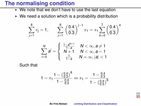
The normalising conditionI We note that we don’t have to use the last equationI We need a solution which is a probability distribution
8∑j=1
πj = 1,8∑
j=1
(0.40.3
)j−1
π1 = π1
7∑k=0
(0.40.3
)k
N∑i=0
ai =
1−aN+1
1−a N <∞,a 6= 1N + 1 N <∞,a = 1
11−a N =∞, |a| < 1
Such that
1 = π11−
(0.40.3
)8
1− 0.40.3
⇔ π1 =1− 0.4
0.3
1−(0.4
0.3
)8
Bo Friis Nielsen Limiting Distribution and Classification

The solution of π = πP
I More or less straightforward, but one problemI if x is a solution such that x = xP then obviously
(kx) = (kx)P is also a solution.I Recall the definition of eigenvalues/eigen vectorsI If Ay = λy we say that λ is an eigenvalue of A with an
associated eigenvector y . Here y is a right eigenvector,there is also a left eigenvector
Bo Friis Nielsen Limiting Distribution and Classification

The solution of π = πP
I More or less straightforward,
but one problemI if x is a solution such that x = xP then obviously
(kx) = (kx)P is also a solution.I Recall the definition of eigenvalues/eigen vectorsI If Ay = λy we say that λ is an eigenvalue of A with an
associated eigenvector y . Here y is a right eigenvector,there is also a left eigenvector
Bo Friis Nielsen Limiting Distribution and Classification

The solution of π = πP
I More or less straightforward, but one problem
I if x is a solution such that x = xP then obviously(kx) = (kx)P is also a solution.
I Recall the definition of eigenvalues/eigen vectorsI If Ay = λy we say that λ is an eigenvalue of A with an
associated eigenvector y . Here y is a right eigenvector,there is also a left eigenvector
Bo Friis Nielsen Limiting Distribution and Classification

The solution of π = πP
I More or less straightforward, but one problemI if x is a solution such that x = xP
then obviously(kx) = (kx)P is also a solution.
I Recall the definition of eigenvalues/eigen vectorsI If Ay = λy we say that λ is an eigenvalue of A with an
associated eigenvector y . Here y is a right eigenvector,there is also a left eigenvector
Bo Friis Nielsen Limiting Distribution and Classification
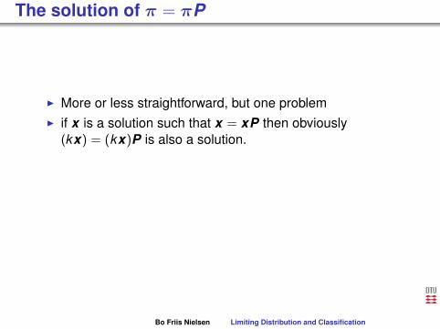
The solution of π = πP
I More or less straightforward, but one problemI if x is a solution such that x = xP then obviously
(kx) = (kx)P is also a solution.
I Recall the definition of eigenvalues/eigen vectorsI If Ay = λy we say that λ is an eigenvalue of A with an
associated eigenvector y . Here y is a right eigenvector,there is also a left eigenvector
Bo Friis Nielsen Limiting Distribution and Classification

The solution of π = πP
I More or less straightforward, but one problemI if x is a solution such that x = xP then obviously
(kx) = (kx)P is also a solution.I Recall the definition of eigenvalues/eigen vectors
I If Ay = λy we say that λ is an eigenvalue of A with anassociated eigenvector y . Here y is a right eigenvector,there is also a left eigenvector
Bo Friis Nielsen Limiting Distribution and Classification

The solution of π = πP
I More or less straightforward, but one problemI if x is a solution such that x = xP then obviously
(kx) = (kx)P is also a solution.I Recall the definition of eigenvalues/eigen vectorsI If Ay = λy we say that λ is an eigenvalue of A with an
associated eigenvector y . Here y is a right eigenvector,there is also a left eigenvector
Bo Friis Nielsen Limiting Distribution and Classification

The solution of π = πP continued
I The vector π is a left eigenvector of P.
I The main theorem says that there is a unique eigenvectorassociated with the eigenvalue 1 of P
I In practice this means that the we can only solve but anormalising condition
I But we have the normalising condition by∑
j πj = 1 thiscan expressed as π1 = 1. Where
1 =
11...1
Bo Friis Nielsen Limiting Distribution and Classification

The solution of π = πP continued
I The vector π is a left eigenvector of P.I The main theorem says that there is a unique eigenvector
associated with the eigenvalue 1 of P
I In practice this means that the we can only solve but anormalising condition
I But we have the normalising condition by∑
j πj = 1 thiscan expressed as π1 = 1. Where
1 =
11...1
Bo Friis Nielsen Limiting Distribution and Classification

The solution of π = πP continued
I The vector π is a left eigenvector of P.I The main theorem says that there is a unique eigenvector
associated with the eigenvalue 1 of PI In practice this means that the we can only solve but a
normalising condition
I But we have the normalising condition by∑
j πj = 1 thiscan expressed as π1 = 1. Where
1 =
11...1
Bo Friis Nielsen Limiting Distribution and Classification

The solution of π = πP continued
I The vector π is a left eigenvector of P.I The main theorem says that there is a unique eigenvector
associated with the eigenvalue 1 of PI In practice this means that the we can only solve but a
normalising conditionI But we have the normalising condition by
∑j πj = 1
thiscan expressed as π1 = 1. Where
1 =
11...1
Bo Friis Nielsen Limiting Distribution and Classification

The solution of π = πP continued
I The vector π is a left eigenvector of P.I The main theorem says that there is a unique eigenvector
associated with the eigenvalue 1 of PI In practice this means that the we can only solve but a
normalising conditionI But we have the normalising condition by
∑j πj = 1 this
can expressed as π1 = 1. Where
1 =
11...1
Bo Friis Nielsen Limiting Distribution and Classification

Roles of the solution to π = πP
For an irreducible Markov chain, (the condition we need toverify)
I The stationary solution. If p(0) = π then p(n) = π for all n.I The limiting distribution, i.e. p(n) → π for n→∞ (the
Markov chain has to be aperiodic too). Also p(n)ij → πj .
I The mean recurrence time for state i is µi =1πi
.I The mean number of visits in state j between two
successive visits to state i is πjπi
.I The long run average probability of finding the Markov
chain in state i is πi . πi = limn→∞1n∑n
k=1 p(k)i also true for
periodic chains.
Bo Friis Nielsen Limiting Distribution and Classification

Roles of the solution to π = πP
For an irreducible Markov chain, (the condition we need toverify)I The stationary solution.
If p(0) = π then p(n) = π for all n.I The limiting distribution, i.e. p(n) → π for n→∞ (the
Markov chain has to be aperiodic too). Also p(n)ij → πj .
I The mean recurrence time for state i is µi =1πi
.I The mean number of visits in state j between two
successive visits to state i is πjπi
.I The long run average probability of finding the Markov
chain in state i is πi . πi = limn→∞1n∑n
k=1 p(k)i also true for
periodic chains.
Bo Friis Nielsen Limiting Distribution and Classification

Roles of the solution to π = πP
For an irreducible Markov chain, (the condition we need toverify)I The stationary solution. If p(0) = π then p(n) = π for all n.
I The limiting distribution, i.e. p(n) → π for n→∞ (theMarkov chain has to be aperiodic too). Also p(n)
ij → πj .I The mean recurrence time for state i is µi =
1πi
.I The mean number of visits in state j between two
successive visits to state i is πjπi
.I The long run average probability of finding the Markov
chain in state i is πi . πi = limn→∞1n∑n
k=1 p(k)i also true for
periodic chains.
Bo Friis Nielsen Limiting Distribution and Classification

Roles of the solution to π = πP
For an irreducible Markov chain, (the condition we need toverify)I The stationary solution. If p(0) = π then p(n) = π for all n.I The limiting distribution,
i.e. p(n) → π for n→∞ (theMarkov chain has to be aperiodic too). Also p(n)
ij → πj .I The mean recurrence time for state i is µi =
1πi
.I The mean number of visits in state j between two
successive visits to state i is πjπi
.I The long run average probability of finding the Markov
chain in state i is πi . πi = limn→∞1n∑n
k=1 p(k)i also true for
periodic chains.
Bo Friis Nielsen Limiting Distribution and Classification

Roles of the solution to π = πP
For an irreducible Markov chain, (the condition we need toverify)I The stationary solution. If p(0) = π then p(n) = π for all n.I The limiting distribution, i.e. p(n)
→ π for n→∞ (theMarkov chain has to be aperiodic too). Also p(n)
ij → πj .I The mean recurrence time for state i is µi =
1πi
.I The mean number of visits in state j between two
successive visits to state i is πjπi
.I The long run average probability of finding the Markov
chain in state i is πi . πi = limn→∞1n∑n
k=1 p(k)i also true for
periodic chains.
Bo Friis Nielsen Limiting Distribution and Classification
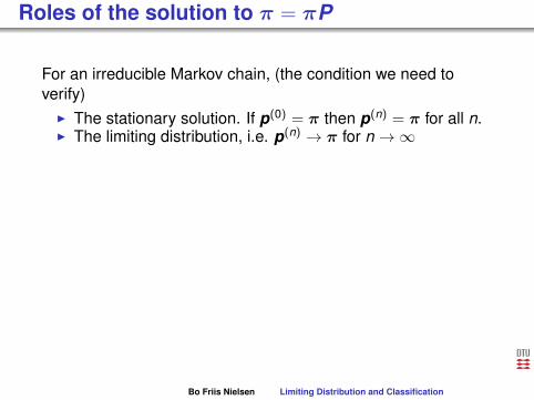
Roles of the solution to π = πP
For an irreducible Markov chain, (the condition we need toverify)I The stationary solution. If p(0) = π then p(n) = π for all n.I The limiting distribution, i.e. p(n) → π for n→∞
(theMarkov chain has to be aperiodic too). Also p(n)
ij → πj .I The mean recurrence time for state i is µi =
1πi
.I The mean number of visits in state j between two
successive visits to state i is πjπi
.I The long run average probability of finding the Markov
chain in state i is πi . πi = limn→∞1n∑n
k=1 p(k)i also true for
periodic chains.
Bo Friis Nielsen Limiting Distribution and Classification

Roles of the solution to π = πP
For an irreducible Markov chain, (the condition we need toverify)I The stationary solution. If p(0) = π then p(n) = π for all n.I The limiting distribution, i.e. p(n) → π for n→∞ (the
Markov chain has to be aperiodic too).
Also p(n)ij → πj .
I The mean recurrence time for state i is µi =1πi
.I The mean number of visits in state j between two
successive visits to state i is πjπi
.I The long run average probability of finding the Markov
chain in state i is πi . πi = limn→∞1n∑n
k=1 p(k)i also true for
periodic chains.
Bo Friis Nielsen Limiting Distribution and Classification

Roles of the solution to π = πP
For an irreducible Markov chain, (the condition we need toverify)I The stationary solution. If p(0) = π then p(n) = π for all n.I The limiting distribution, i.e. p(n) → π for n→∞ (the
Markov chain has to be aperiodic too). Also p(n)ij
→ πj .I The mean recurrence time for state i is µi =
1πi
.I The mean number of visits in state j between two
successive visits to state i is πjπi
.I The long run average probability of finding the Markov
chain in state i is πi . πi = limn→∞1n∑n
k=1 p(k)i also true for
periodic chains.
Bo Friis Nielsen Limiting Distribution and Classification

Roles of the solution to π = πP
For an irreducible Markov chain, (the condition we need toverify)I The stationary solution. If p(0) = π then p(n) = π for all n.I The limiting distribution, i.e. p(n) → π for n→∞ (the
Markov chain has to be aperiodic too). Also p(n)ij → πj .
I The mean recurrence time for state i is µi =1πi
.I The mean number of visits in state j between two
successive visits to state i is πjπi
.I The long run average probability of finding the Markov
chain in state i is πi . πi = limn→∞1n∑n
k=1 p(k)i also true for
periodic chains.
Bo Friis Nielsen Limiting Distribution and Classification

Roles of the solution to π = πP
For an irreducible Markov chain, (the condition we need toverify)I The stationary solution. If p(0) = π then p(n) = π for all n.I The limiting distribution, i.e. p(n) → π for n→∞ (the
Markov chain has to be aperiodic too). Also p(n)ij → πj .
I The mean recurrence time for state i
is µi =1πi
.I The mean number of visits in state j between two
successive visits to state i is πjπi
.I The long run average probability of finding the Markov
chain in state i is πi . πi = limn→∞1n∑n
k=1 p(k)i also true for
periodic chains.
Bo Friis Nielsen Limiting Distribution and Classification

Roles of the solution to π = πP
For an irreducible Markov chain, (the condition we need toverify)I The stationary solution. If p(0) = π then p(n) = π for all n.I The limiting distribution, i.e. p(n) → π for n→∞ (the
Markov chain has to be aperiodic too). Also p(n)ij → πj .
I The mean recurrence time for state i is µi
= 1πi
.I The mean number of visits in state j between two
successive visits to state i is πjπi
.I The long run average probability of finding the Markov
chain in state i is πi . πi = limn→∞1n∑n
k=1 p(k)i also true for
periodic chains.
Bo Friis Nielsen Limiting Distribution and Classification

Roles of the solution to π = πP
For an irreducible Markov chain, (the condition we need toverify)I The stationary solution. If p(0) = π then p(n) = π for all n.I The limiting distribution, i.e. p(n) → π for n→∞ (the
Markov chain has to be aperiodic too). Also p(n)ij → πj .
I The mean recurrence time for state i is µi =1πi
.
I The mean number of visits in state j between twosuccessive visits to state i is πj
πi.
I The long run average probability of finding the Markovchain in state i is πi . πi = limn→∞
1n∑n
k=1 p(k)i also true for
periodic chains.
Bo Friis Nielsen Limiting Distribution and Classification

Roles of the solution to π = πP
For an irreducible Markov chain, (the condition we need toverify)I The stationary solution. If p(0) = π then p(n) = π for all n.I The limiting distribution, i.e. p(n) → π for n→∞ (the
Markov chain has to be aperiodic too). Also p(n)ij → πj .
I The mean recurrence time for state i is µi =1πi
.I The mean number of visits in state j between two
successive visits to state i
is πjπi
.I The long run average probability of finding the Markov
chain in state i is πi . πi = limn→∞1n∑n
k=1 p(k)i also true for
periodic chains.
Bo Friis Nielsen Limiting Distribution and Classification

Roles of the solution to π = πP
For an irreducible Markov chain, (the condition we need toverify)I The stationary solution. If p(0) = π then p(n) = π for all n.I The limiting distribution, i.e. p(n) → π for n→∞ (the
Markov chain has to be aperiodic too). Also p(n)ij → πj .
I The mean recurrence time for state i is µi =1πi
.I The mean number of visits in state j between two
successive visits to state i is πjπi
.
I The long run average probability of finding the Markovchain in state i is πi . πi = limn→∞
1n∑n
k=1 p(k)i also true for
periodic chains.
Bo Friis Nielsen Limiting Distribution and Classification

Roles of the solution to π = πP
For an irreducible Markov chain, (the condition we need toverify)I The stationary solution. If p(0) = π then p(n) = π for all n.I The limiting distribution, i.e. p(n) → π for n→∞ (the
Markov chain has to be aperiodic too). Also p(n)ij → πj .
I The mean recurrence time for state i is µi =1πi
.I The mean number of visits in state j between two
successive visits to state i is πjπi
.I The long run average probability of finding the Markov
chain in state i is πi .
πi = limn→∞1n∑n
k=1 p(k)i also true for
periodic chains.
Bo Friis Nielsen Limiting Distribution and Classification

Roles of the solution to π = πP
For an irreducible Markov chain, (the condition we need toverify)I The stationary solution. If p(0) = π then p(n) = π for all n.I The limiting distribution, i.e. p(n) → π for n→∞ (the
Markov chain has to be aperiodic too). Also p(n)ij → πj .
I The mean recurrence time for state i is µi =1πi
.I The mean number of visits in state j between two
successive visits to state i is πjπi
.I The long run average probability of finding the Markov
chain in state i is πi . πi = limn→∞1n∑n
k=1 p(k)i
also true forperiodic chains.
Bo Friis Nielsen Limiting Distribution and Classification
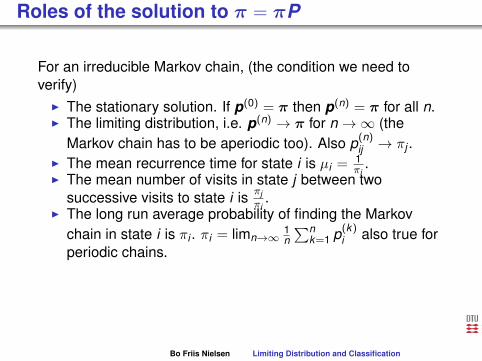
Roles of the solution to π = πP
For an irreducible Markov chain, (the condition we need toverify)I The stationary solution. If p(0) = π then p(n) = π for all n.I The limiting distribution, i.e. p(n) → π for n→∞ (the
Markov chain has to be aperiodic too). Also p(n)ij → πj .
I The mean recurrence time for state i is µi =1πi
.I The mean number of visits in state j between two
successive visits to state i is πjπi
.I The long run average probability of finding the Markov
chain in state i is πi . πi = limn→∞1n∑n
k=1 p(k)i also true for
periodic chains.
Bo Friis Nielsen Limiting Distribution and Classification

Example (null-recurrent) chain
P =
p1 p2 p3 p4 p5 . . .1 0 0 0 0 . . .0 1 0 0 0 . . .0 0 1 0 0 . . .0 0 0 1 0 . . .0 0 0 0 1 . . .. . . . . . . . . . . . . . . . . .
For pj > 0 the chain is obviously irreducible.The main theorem tells us that we can investigate directly forπ = πP.
π1 = π1p1 + π2 π2 = π1p2 + π3 πj = π1pj + πj+1
Bo Friis Nielsen Limiting Distribution and Classification

Example (null-recurrent) chain
P =
p1 p2 p3 p4 p5 . . .1 0 0 0 0 . . .0 1 0 0 0 . . .0 0 1 0 0 . . .0 0 0 1 0 . . .0 0 0 0 1 . . .. . . . . . . . . . . . . . . . . .
For pj > 0 the chain is obviously irreducible.
The main theorem tells us that we can investigate directly forπ = πP.
π1 = π1p1 + π2 π2 = π1p2 + π3 πj = π1pj + πj+1
Bo Friis Nielsen Limiting Distribution and Classification
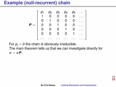
Example (null-recurrent) chain
P =
p1 p2 p3 p4 p5 . . .1 0 0 0 0 . . .0 1 0 0 0 . . .0 0 1 0 0 . . .0 0 0 1 0 . . .0 0 0 0 1 . . .. . . . . . . . . . . . . . . . . .
For pj > 0 the chain is obviously irreducible.The main theorem tells us that we can investigate directly forπ = πP.
π1 = π1p1 + π2 π2 = π1p2 + π3 πj = π1pj + πj+1
Bo Friis Nielsen Limiting Distribution and Classification

Example (null-recurrent) chain
P =
p1 p2 p3 p4 p5 . . .1 0 0 0 0 . . .0 1 0 0 0 . . .0 0 1 0 0 . . .0 0 0 1 0 . . .0 0 0 0 1 . . .. . . . . . . . . . . . . . . . . .
For pj > 0 the chain is obviously irreducible.The main theorem tells us that we can investigate directly forπ = πP.
π1
= π1p1 + π2 π2 = π1p2 + π3 πj = π1pj + πj+1
Bo Friis Nielsen Limiting Distribution and Classification

Example (null-recurrent) chain
P =
p1 p2 p3 p4 p5 . . .1 0 0 0 0 . . .0 1 0 0 0 . . .0 0 1 0 0 . . .0 0 0 1 0 . . .0 0 0 0 1 . . .. . . . . . . . . . . . . . . . . .
For pj > 0 the chain is obviously irreducible.The main theorem tells us that we can investigate directly forπ = πP.
π1 = π1
p1 + π2 π2 = π1p2 + π3 πj = π1pj + πj+1
Bo Friis Nielsen Limiting Distribution and Classification

Example (null-recurrent) chain
P =
p1 p2 p3 p4 p5 . . .1 0 0 0 0 . . .0 1 0 0 0 . . .0 0 1 0 0 . . .0 0 0 1 0 . . .0 0 0 0 1 . . .. . . . . . . . . . . . . . . . . .
For pj > 0 the chain is obviously irreducible.The main theorem tells us that we can investigate directly forπ = πP.
π1 = π1p1 +
π2 π2 = π1p2 + π3 πj = π1pj + πj+1
Bo Friis Nielsen Limiting Distribution and Classification

Example (null-recurrent) chain
P =
p1 p2 p3 p4 p5 . . .1 0 0 0 0 . . .0 1 0 0 0 . . .0 0 1 0 0 . . .0 0 0 1 0 . . .0 0 0 0 1 . . .. . . . . . . . . . . . . . . . . .
For pj > 0 the chain is obviously irreducible.The main theorem tells us that we can investigate directly forπ = πP.
π1 = π1p1 + π2
π2 = π1p2 + π3 πj = π1pj + πj+1
Bo Friis Nielsen Limiting Distribution and Classification

Example (null-recurrent) chain
P =
p1 p2 p3 p4 p5 . . .1 0 0 0 0 . . .0 1 0 0 0 . . .0 0 1 0 0 . . .0 0 0 1 0 . . .0 0 0 0 1 . . .. . . . . . . . . . . . . . . . . .
For pj > 0 the chain is obviously irreducible.The main theorem tells us that we can investigate directly forπ = πP.
π1 = π1p1 + π2 π2
= π1p2 + π3 πj = π1pj + πj+1
Bo Friis Nielsen Limiting Distribution and Classification
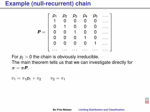
Example (null-recurrent) chain
P =
p1 p2 p3 p4 p5 . . .1 0 0 0 0 . . .0 1 0 0 0 . . .0 0 1 0 0 . . .0 0 0 1 0 . . .0 0 0 0 1 . . .. . . . . . . . . . . . . . . . . .
For pj > 0 the chain is obviously irreducible.The main theorem tells us that we can investigate directly forπ = πP.
π1 = π1p1 + π2 π2 = π1
p2 + π3 πj = π1pj + πj+1
Bo Friis Nielsen Limiting Distribution and Classification

Example (null-recurrent) chain
P =
p1 p2 p3 p4 p5 . . .1 0 0 0 0 . . .0 1 0 0 0 . . .0 0 1 0 0 . . .0 0 0 1 0 . . .0 0 0 0 1 . . .. . . . . . . . . . . . . . . . . .
For pj > 0 the chain is obviously irreducible.The main theorem tells us that we can investigate directly forπ = πP.
π1 = π1p1 + π2 π2 = π1p2
+ π3 πj = π1pj + πj+1
Bo Friis Nielsen Limiting Distribution and Classification

Example (null-recurrent) chain
P =
p1 p2 p3 p4 p5 . . .1 0 0 0 0 . . .0 1 0 0 0 . . .0 0 1 0 0 . . .0 0 0 1 0 . . .0 0 0 0 1 . . .. . . . . . . . . . . . . . . . . .
For pj > 0 the chain is obviously irreducible.The main theorem tells us that we can investigate directly forπ = πP.
π1 = π1p1 + π2 π2 = π1p2 + π3
πj = π1pj + πj+1
Bo Friis Nielsen Limiting Distribution and Classification
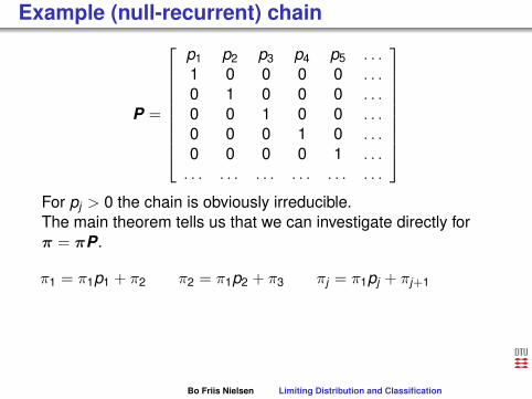
Example (null-recurrent) chain
P =
p1 p2 p3 p4 p5 . . .1 0 0 0 0 . . .0 1 0 0 0 . . .0 0 1 0 0 . . .0 0 0 1 0 . . .0 0 0 0 1 . . .. . . . . . . . . . . . . . . . . .
For pj > 0 the chain is obviously irreducible.The main theorem tells us that we can investigate directly forπ = πP.
π1 = π1p1 + π2 π2 = π1p2 + π3 πj = π1pj + πj+1
Bo Friis Nielsen Limiting Distribution and Classification

π1 = π1p1 + π2 π2 = π1p2 + π3 πj = π1pj + πj+1
we get
π2 = (1−p1)π1 π3 = (1−p1−p2)π1 πj = (1−p1 · · ·−pj−1)π1
πj = (1− p1 · · · − pj−1)π1 ⇔ πj = π1
1−j−1∑i=1
pi
⇔ πj = π1
∞∑i=j
pi
Normalisation
∞∑j=1
πj = 1∞∑
j=1
π1
∞∑i=j
pi = π1
∞∑i=1
i∑j=1
pi = π1
∞∑i=1
ipi
Bo Friis Nielsen Limiting Distribution and Classification

π1 = π1p1 + π2 π2 = π1p2 + π3 πj = π1pj + πj+1
we get
π2
= (1−p1)π1 π3 = (1−p1−p2)π1 πj = (1−p1 · · ·−pj−1)π1
πj = (1− p1 · · · − pj−1)π1 ⇔ πj = π1
1−j−1∑i=1
pi
⇔ πj = π1
∞∑i=j
pi
Normalisation
∞∑j=1
πj = 1∞∑
j=1
π1
∞∑i=j
pi = π1
∞∑i=1
i∑j=1
pi = π1
∞∑i=1
ipi
Bo Friis Nielsen Limiting Distribution and Classification

π1 = π1p1 + π2 π2 = π1p2 + π3 πj = π1pj + πj+1
we get
π2 = (1−p1)π1
π3 = (1−p1−p2)π1 πj = (1−p1 · · ·−pj−1)π1
πj = (1− p1 · · · − pj−1)π1 ⇔ πj = π1
1−j−1∑i=1
pi
⇔ πj = π1
∞∑i=j
pi
Normalisation
∞∑j=1
πj = 1∞∑
j=1
π1
∞∑i=j
pi = π1
∞∑i=1
i∑j=1
pi = π1
∞∑i=1
ipi
Bo Friis Nielsen Limiting Distribution and Classification

π1 = π1p1 + π2 π2 = π1p2 + π3 πj = π1pj + πj+1
we get
π2 = (1−p1)π1 π3 = (1−p1−p2)π1
πj = (1−p1 · · ·−pj−1)π1
πj = (1− p1 · · · − pj−1)π1 ⇔ πj = π1
1−j−1∑i=1
pi
⇔ πj = π1
∞∑i=j
pi
Normalisation
∞∑j=1
πj = 1∞∑
j=1
π1
∞∑i=j
pi = π1
∞∑i=1
i∑j=1
pi = π1
∞∑i=1
ipi
Bo Friis Nielsen Limiting Distribution and Classification

π1 = π1p1 + π2 π2 = π1p2 + π3 πj = π1pj + πj+1
we get
π2 = (1−p1)π1 π3 = (1−p1−p2)π1 πj = (1−p1 · · ·−pj−1)π1
πj = (1− p1 · · · − pj−1)π1 ⇔ πj = π1
1−j−1∑i=1
pi
⇔ πj = π1
∞∑i=j
pi
Normalisation
∞∑j=1
πj = 1∞∑
j=1
π1
∞∑i=j
pi = π1
∞∑i=1
i∑j=1
pi = π1
∞∑i=1
ipi
Bo Friis Nielsen Limiting Distribution and Classification
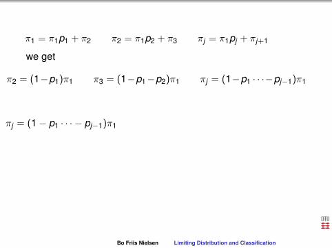
π1 = π1p1 + π2 π2 = π1p2 + π3 πj = π1pj + πj+1
we get
π2 = (1−p1)π1 π3 = (1−p1−p2)π1 πj = (1−p1 · · ·−pj−1)π1
πj = (1− p1 · · · − pj−1)π1
⇔ πj = π1
1−j−1∑i=1
pi
⇔ πj = π1
∞∑i=j
pi
Normalisation
∞∑j=1
πj = 1∞∑
j=1
π1
∞∑i=j
pi = π1
∞∑i=1
i∑j=1
pi = π1
∞∑i=1
ipi
Bo Friis Nielsen Limiting Distribution and Classification

π1 = π1p1 + π2 π2 = π1p2 + π3 πj = π1pj + πj+1
we get
π2 = (1−p1)π1 π3 = (1−p1−p2)π1 πj = (1−p1 · · ·−pj−1)π1
πj = (1− p1 · · · − pj−1)π1 ⇔ πj = π1
1−j−1∑i=1
pi
⇔ πj = π1
∞∑i=j
pi
Normalisation
∞∑j=1
πj = 1∞∑
j=1
π1
∞∑i=j
pi = π1
∞∑i=1
i∑j=1
pi = π1
∞∑i=1
ipi
Bo Friis Nielsen Limiting Distribution and Classification

π1 = π1p1 + π2 π2 = π1p2 + π3 πj = π1pj + πj+1
we get
π2 = (1−p1)π1 π3 = (1−p1−p2)π1 πj = (1−p1 · · ·−pj−1)π1
πj = (1− p1 · · · − pj−1)π1 ⇔ πj = π1
1−j−1∑i=1
pi
⇔ πj = π1
∞∑i=j
pi
Normalisation
∞∑j=1
πj = 1
∞∑j=1
π1
∞∑i=j
pi = π1
∞∑i=1
i∑j=1
pi = π1
∞∑i=1
ipi
Bo Friis Nielsen Limiting Distribution and Classification
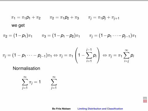
π1 = π1p1 + π2 π2 = π1p2 + π3 πj = π1pj + πj+1
we get
π2 = (1−p1)π1 π3 = (1−p1−p2)π1 πj = (1−p1 · · ·−pj−1)π1
πj = (1− p1 · · · − pj−1)π1 ⇔ πj = π1
1−j−1∑i=1
pi
⇔ πj = π1
∞∑i=j
pi
Normalisation
∞∑j=1
πj = 1∞∑
j=1
π1
∞∑i=j
pi = π1
∞∑i=1
i∑j=1
pi = π1
∞∑i=1
ipi
Bo Friis Nielsen Limiting Distribution and Classification

π1 = π1p1 + π2 π2 = π1p2 + π3 πj = π1pj + πj+1
we get
π2 = (1−p1)π1 π3 = (1−p1−p2)π1 πj = (1−p1 · · ·−pj−1)π1
πj = (1− p1 · · · − pj−1)π1 ⇔ πj = π1
1−j−1∑i=1
pi
⇔ πj = π1
∞∑i=j
pi
Normalisation
∞∑j=1
πj = 1∞∑
j=1
π1
∞∑i=j
pi =
π1
∞∑i=1
i∑j=1
pi = π1
∞∑i=1
ipi
Bo Friis Nielsen Limiting Distribution and Classification

π1 = π1p1 + π2 π2 = π1p2 + π3 πj = π1pj + πj+1
we get
π2 = (1−p1)π1 π3 = (1−p1−p2)π1 πj = (1−p1 · · ·−pj−1)π1
πj = (1− p1 · · · − pj−1)π1 ⇔ πj = π1
1−j−1∑i=1
pi
⇔ πj = π1
∞∑i=j
pi
Normalisation
∞∑j=1
πj = 1∞∑
j=1
π1
∞∑i=j
pi = π1
∞∑i=1
i∑j=1
pi
= π1
∞∑i=1
ipi
Bo Friis Nielsen Limiting Distribution and Classification

π1 = π1p1 + π2 π2 = π1p2 + π3 πj = π1pj + πj+1
we get
π2 = (1−p1)π1 π3 = (1−p1−p2)π1 πj = (1−p1 · · ·−pj−1)π1
πj = (1− p1 · · · − pj−1)π1 ⇔ πj = π1
1−j−1∑i=1
pi
⇔ πj = π1
∞∑i=j
pi
Normalisation
∞∑j=1
πj = 1∞∑
j=1
π1
∞∑i=j
pi = π1
∞∑i=1
i∑j=1
pi = π1
∞∑i=1
ipi
Bo Friis Nielsen Limiting Distribution and Classification
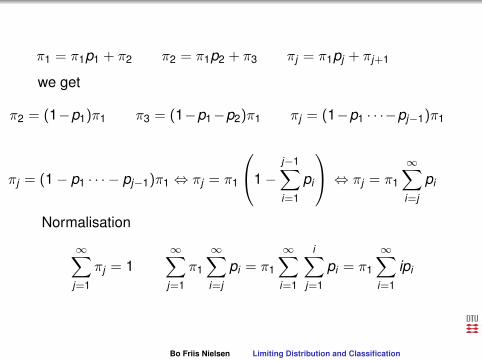
π1 = π1p1 + π2 π2 = π1p2 + π3 πj = π1pj + πj+1
we get
π2 = (1−p1)π1 π3 = (1−p1−p2)π1 πj = (1−p1 · · ·−pj−1)π1
πj = (1− p1 · · · − pj−1)π1 ⇔ πj = π1
1−j−1∑i=1
pi
⇔ πj = π1
∞∑i=j
pi
Normalisation
∞∑j=1
πj = 1∞∑
j=1
π1
∞∑i=j
pi = π1
∞∑i=1
i∑j=1
pi = π1
∞∑i=1
ipi
Bo Friis Nielsen Limiting Distribution and Classification
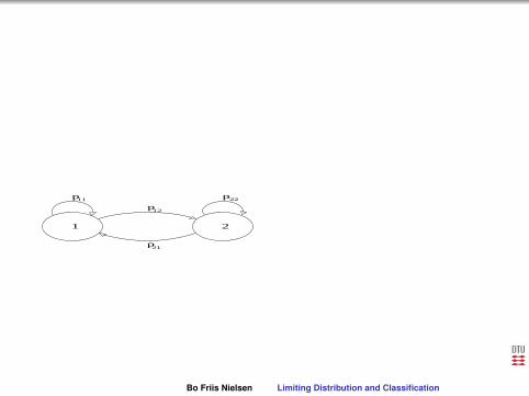
1 2
p
p
pp11
12
22
21
P =
[p11 p12p21 p22
]
Bo Friis Nielsen Limiting Distribution and Classification

1 2
p
p
pp11
12
22
21
P =
[p11 p12p21 p22
]
Bo Friis Nielsen Limiting Distribution and Classification
Reversible Markov chains
I Solve sequence of linear equations instead of the wholesystem
I Local balance in probability flow as opposed to globalbalance
I Nice theoretical construction
Bo Friis Nielsen Limiting Distribution and Classification

Reversible Markov chains
I Solve sequence of linear equations instead of the wholesystem
I Local balance in probability flow as opposed to globalbalance
I Nice theoretical construction
Bo Friis Nielsen Limiting Distribution and Classification
Reversible Markov chains
I Solve sequence of linear equations instead of the wholesystem
I Local balance in probability flow as opposed to globalbalance
I Nice theoretical construction
Bo Friis Nielsen Limiting Distribution and Classification

Bo Friis Nielsen Limiting Distribution and Classification
Local balance equations
πi
=∑
j
πjpji πi · 1 =∑
j
πjpji πi∑
j
pij =∑
j
πjpji
∑j
πipij =∑
j
πjpji
Term for term we getπipij = πjpji
If they are fulfilled for each i and j , the global balance equationscan be obtained by summation.
Bo Friis Nielsen Limiting Distribution and Classification
Local balance equations
πi =∑
j
πj
pji πi · 1 =∑
j
πjpji πi∑
j
pij =∑
j
πjpji
∑j
πipij =∑
j
πjpji
Term for term we getπipij = πjpji
If they are fulfilled for each i and j , the global balance equationscan be obtained by summation.
Bo Friis Nielsen Limiting Distribution and Classification

Local balance equations
πi =∑
j
πjpji
πi · 1 =∑
j
πjpji πi∑
j
pij =∑
j
πjpji
∑j
πipij =∑
j
πjpji
Term for term we getπipij = πjpji
If they are fulfilled for each i and j , the global balance equationscan be obtained by summation.
Bo Friis Nielsen Limiting Distribution and Classification

Local balance equations
πi =∑
j
πjpji πi · 1
=∑
j
πjpji πi∑
j
pij =∑
j
πjpji
∑j
πipij =∑
j
πjpji
Term for term we getπipij = πjpji
If they are fulfilled for each i and j , the global balance equationscan be obtained by summation.
Bo Friis Nielsen Limiting Distribution and Classification

Local balance equations
πi =∑
j
πjpji πi · 1 =∑
j
πjpji
πi∑
j
pij =∑
j
πjpji
∑j
πipij =∑
j
πjpji
Term for term we getπipij = πjpji
If they are fulfilled for each i and j , the global balance equationscan be obtained by summation.
Bo Friis Nielsen Limiting Distribution and Classification
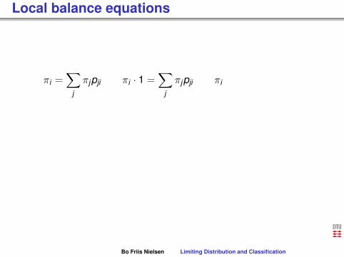
Local balance equations
πi =∑
j
πjpji πi · 1 =∑
j
πjpji πi
∑j
pij =∑
j
πjpji
∑j
πipij =∑
j
πjpji
Term for term we getπipij = πjpji
If they are fulfilled for each i and j , the global balance equationscan be obtained by summation.
Bo Friis Nielsen Limiting Distribution and Classification

Local balance equations
πi =∑
j
πjpji πi · 1 =∑
j
πjpji πi∑
j
pij
=∑
j
πjpji
∑j
πipij =∑
j
πjpji
Term for term we getπipij = πjpji
If they are fulfilled for each i and j , the global balance equationscan be obtained by summation.
Bo Friis Nielsen Limiting Distribution and Classification

Local balance equations
πi =∑
j
πjpji πi · 1 =∑
j
πjpji πi∑
j
pij =∑
j
πjpji
∑j
πipij =∑
j
πjpji
Term for term we getπipij = πjpji
If they are fulfilled for each i and j , the global balance equationscan be obtained by summation.
Bo Friis Nielsen Limiting Distribution and Classification

Local balance equations
πi =∑
j
πjpji πi · 1 =∑
j
πjpji πi∑
j
pij =∑
j
πjpji
∑j
πipij =∑
j
πjpji
Term for term we getπipij = πjpji
If they are fulfilled for each i and j , the global balance equationscan be obtained by summation.
Bo Friis Nielsen Limiting Distribution and Classification

Local balance equations
πi =∑
j
πjpji πi · 1 =∑
j
πjpji πi∑
j
pij =∑
j
πjpji
∑j
πipij =∑
j
πjpji
Term for term we get
πipij = πjpji
If they are fulfilled for each i and j , the global balance equationscan be obtained by summation.
Bo Friis Nielsen Limiting Distribution and Classification

Local balance equations
πi =∑
j
πjpji πi · 1 =∑
j
πjpji πi∑
j
pij =∑
j
πjpji
∑j
πipij =∑
j
πjpji
Term for term we getπipij = πjpji
If they are fulfilled for each i and j , the global balance equationscan be obtained by summation.
Bo Friis Nielsen Limiting Distribution and Classification

Local balance equations
πi =∑
j
πjpji πi · 1 =∑
j
πjpji πi∑
j
pij =∑
j
πjpji
∑j
πipij =∑
j
πjpji
Term for term we getπipij = πjpji
If they are fulfilled for each i and j , the global balance equationscan be obtained by summation.
Bo Friis Nielsen Limiting Distribution and Classification
Why reversible?
P{Xn−1 = i ∩ Xn = j} = P{Xn−1 = i}P{Xn = j |Xn−1 = i}
= P{Xn−1 = i}pij
and for a stationary chain
πipij
For a reversible chain (local balance) this is πipij = πjpji =P{Xn−1 = j}P{Xn = i |Xn−1 = j} = P{Xn−1 = j ∩ Xn = i} thereversed sequence.
Bo Friis Nielsen Limiting Distribution and Classification

Why reversible?
P{Xn−1 = i ∩ Xn = j}
= P{Xn−1 = i}P{Xn = j |Xn−1 = i}
= P{Xn−1 = i}pij
and for a stationary chain
πipij
For a reversible chain (local balance) this is πipij = πjpji =P{Xn−1 = j}P{Xn = i |Xn−1 = j} = P{Xn−1 = j ∩ Xn = i} thereversed sequence.
Bo Friis Nielsen Limiting Distribution and Classification

Why reversible?
P{Xn−1 = i ∩ Xn = j} = P{Xn−1 = i}
P{Xn = j |Xn−1 = i}
= P{Xn−1 = i}pij
and for a stationary chain
πipij
For a reversible chain (local balance) this is πipij = πjpji =P{Xn−1 = j}P{Xn = i |Xn−1 = j} = P{Xn−1 = j ∩ Xn = i} thereversed sequence.
Bo Friis Nielsen Limiting Distribution and Classification
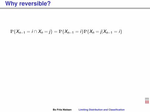
Why reversible?
P{Xn−1 = i ∩ Xn = j} = P{Xn−1 = i}P{Xn = j |Xn−1 = i}
= P{Xn−1 = i}pij
and for a stationary chain
πipij
For a reversible chain (local balance) this is πipij = πjpji =P{Xn−1 = j}P{Xn = i |Xn−1 = j} = P{Xn−1 = j ∩ Xn = i} thereversed sequence.
Bo Friis Nielsen Limiting Distribution and Classification

Why reversible?
P{Xn−1 = i ∩ Xn = j} = P{Xn−1 = i}P{Xn = j |Xn−1 = i}
= P{Xn−1 = i}pij
and for a stationary chain
πipij
For a reversible chain (local balance)
this is πipij = πjpji =P{Xn−1 = j}P{Xn = i |Xn−1 = j} = P{Xn−1 = j ∩ Xn = i} thereversed sequence.
Bo Friis Nielsen Limiting Distribution and Classification

Why reversible?
P{Xn−1 = i ∩ Xn = j} = P{Xn−1 = i}P{Xn = j |Xn−1 = i}
= P{Xn−1 = i}pij
and for a stationary chain
πipij
For a reversible chain (local balance) this is πipij = πjpji
=P{Xn−1 = j}P{Xn = i |Xn−1 = j} = P{Xn−1 = j ∩ Xn = i} thereversed sequence.
Bo Friis Nielsen Limiting Distribution and Classification

Why reversible?
P{Xn−1 = i ∩ Xn = j} = P{Xn−1 = i}P{Xn = j |Xn−1 = i}
= P{Xn−1 = i}pij
and for a stationary chain
πipij
For a reversible chain (local balance) this is πipij = πjpji =P{Xn−1 = j}
P{Xn = i |Xn−1 = j} = P{Xn−1 = j ∩ Xn = i} thereversed sequence.
Bo Friis Nielsen Limiting Distribution and Classification
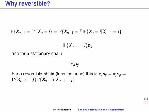
Why reversible?
P{Xn−1 = i ∩ Xn = j} = P{Xn−1 = i}P{Xn = j |Xn−1 = i}
= P{Xn−1 = i}pij
and for a stationary chain
πipij
For a reversible chain (local balance) this is πipij = πjpji =P{Xn−1 = j}P{Xn = i |Xn−1 = j}
= P{Xn−1 = j ∩ Xn = i} thereversed sequence.
Bo Friis Nielsen Limiting Distribution and Classification
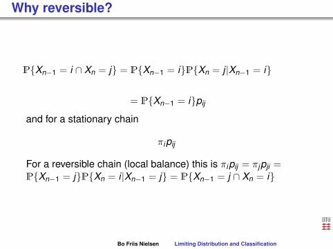
Why reversible?
P{Xn−1 = i ∩ Xn = j} = P{Xn−1 = i}P{Xn = j |Xn−1 = i}
= P{Xn−1 = i}pij
and for a stationary chain
πipij
For a reversible chain (local balance) this is πipij = πjpji =P{Xn−1 = j}P{Xn = i |Xn−1 = j} = P{Xn−1 = j ∩ Xn = i}
thereversed sequence.
Bo Friis Nielsen Limiting Distribution and Classification

Why reversible?
P{Xn−1 = i ∩ Xn = j} = P{Xn−1 = i}P{Xn = j |Xn−1 = i}
= P{Xn−1 = i}pij
and for a stationary chain
πipij
For a reversible chain (local balance) this is πipij = πjpji =P{Xn−1 = j}P{Xn = i |Xn−1 = j} = P{Xn−1 = j ∩ Xn = i} thereversed sequence.
Bo Friis Nielsen Limiting Distribution and Classification

Another look at a similar question
P{Xn−1 = j |Xn = i} = P{Xn−1 = j ∩ Xn = i}P{Xn = i}
=P{Xn−1 = j}P{Xn = i |Xn−1 = j}
P{Xn = i}=P{Xn−1 = j}pji
P{Xn = i}For a stationary chain we get
πjpji
πi
The chain is reversible if P{Xn−1 = j |Xn = i} = pij leading tothe local balance equations
pij =πjpji
πi
Bo Friis Nielsen Limiting Distribution and Classification

Another look at a similar question
P{Xn−1 = j |Xn = i}
=P{Xn−1 = j ∩ Xn = i}
P{Xn = i}
=P{Xn−1 = j}P{Xn = i |Xn−1 = j}
P{Xn = i}=P{Xn−1 = j}pji
P{Xn = i}For a stationary chain we get
πjpji
πi
The chain is reversible if P{Xn−1 = j |Xn = i} = pij leading tothe local balance equations
pij =πjpji
πi
Bo Friis Nielsen Limiting Distribution and Classification

Another look at a similar question
P{Xn−1 = j |Xn = i} = P{Xn−1 = j ∩ Xn = i}
P{Xn = i}
=P{Xn−1 = j}P{Xn = i |Xn−1 = j}
P{Xn = i}=P{Xn−1 = j}pji
P{Xn = i}For a stationary chain we get
πjpji
πi
The chain is reversible if P{Xn−1 = j |Xn = i} = pij leading tothe local balance equations
pij =πjpji
πi
Bo Friis Nielsen Limiting Distribution and Classification

Another look at a similar question
P{Xn−1 = j |Xn = i} = P{Xn−1 = j ∩ Xn = i}P{Xn = i}
=P{Xn−1 = j}P{Xn = i |Xn−1 = j}
P{Xn = i}=P{Xn−1 = j}pji
P{Xn = i}For a stationary chain we get
πjpji
πi
The chain is reversible if P{Xn−1 = j |Xn = i} = pij leading tothe local balance equations
pij =πjpji
πi
Bo Friis Nielsen Limiting Distribution and Classification
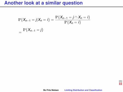
Another look at a similar question
P{Xn−1 = j |Xn = i} = P{Xn−1 = j ∩ Xn = i}P{Xn = i}
=P{Xn−1 = j}
P{Xn = i |Xn−1 = j}P{Xn = i}
=P{Xn−1 = j}pji
P{Xn = i}For a stationary chain we get
πjpji
πi
The chain is reversible if P{Xn−1 = j |Xn = i} = pij leading tothe local balance equations
pij =πjpji
πi
Bo Friis Nielsen Limiting Distribution and Classification

Another look at a similar question
P{Xn−1 = j |Xn = i} = P{Xn−1 = j ∩ Xn = i}P{Xn = i}
=P{Xn−1 = j}P{Xn = i |Xn−1 = j}
P{Xn = i}
=P{Xn−1 = j}pji
P{Xn = i}For a stationary chain we get
πjpji
πi
The chain is reversible if P{Xn−1 = j |Xn = i} = pij leading tothe local balance equations
pij =πjpji
πi
Bo Friis Nielsen Limiting Distribution and Classification
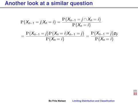
Another look at a similar question
P{Xn−1 = j |Xn = i} = P{Xn−1 = j ∩ Xn = i}P{Xn = i}
=P{Xn−1 = j}P{Xn = i |Xn−1 = j}
P{Xn = i}=P{Xn−1 = j}pji
P{Xn = i}
For a stationary chain we get
πjpji
πi
The chain is reversible if P{Xn−1 = j |Xn = i} = pij leading tothe local balance equations
pij =πjpji
πi
Bo Friis Nielsen Limiting Distribution and Classification

Another look at a similar question
P{Xn−1 = j |Xn = i} = P{Xn−1 = j ∩ Xn = i}P{Xn = i}
=P{Xn−1 = j}P{Xn = i |Xn−1 = j}
P{Xn = i}=P{Xn−1 = j}pji
P{Xn = i}For a stationary chain we get
πjpji
πi
The chain is reversible if P{Xn−1 = j |Xn = i} = pij leading tothe local balance equations
pij =πjpji
πi
Bo Friis Nielsen Limiting Distribution and Classification

Another look at a similar question
P{Xn−1 = j |Xn = i} = P{Xn−1 = j ∩ Xn = i}P{Xn = i}
=P{Xn−1 = j}P{Xn = i |Xn−1 = j}
P{Xn = i}=P{Xn−1 = j}pji
P{Xn = i}For a stationary chain we get
πjpji
πi
The chain is reversible if P{Xn−1 = j |Xn = i} = pij leading tothe local balance equations
pij =πjpji
πi
Bo Friis Nielsen Limiting Distribution and Classification

Exercise 10 (16/12/91 ex.1)
In connection with an examination of the reliability of somesoftware intended for use in control of modern ferries one isinterested in examining a stochastic model of the use of acontrol program.The control program works as " state machine " i.e. it can be ina number of different levels, 4 are considered here. The levelsdepend on the physical state of the ferry. With every shift oftime unit while the program is run, the program will change fromlevel j to level k with probability pjk .
Bo Friis Nielsen Limiting Distribution and Classification

Two possibilities are considered:
The program has no errors and will run continously shifting between the fourlevels.The program has a critical error. In this case it is possible that the error isfound, this happens with probality qi , i = 1, 2, 3, 4 depending on the level.The error will be corrected immediately and the program will from then on bewithout faults.Alternatively the program can stop with a critical error (the ferry will continueto sail, but without control). This happens with probability ri , i = 1, 2, 3, 4.In general qi + ri < 1, a program with errors can thus work and the error isnot nescesarily discovered. It is assumed that detection of an error, as wellas the apperance of a fault happens coincidently with shift between levels.The program starts running in level 1, and it is known that the programcontains one critical error.
Bo Friis Nielsen Limiting Distribution and Classification
Two possibilities are considered:The program has no errors and will run continously shifting between the fourlevels.
The program has a critical error. In this case it is possible that the error isfound, this happens with probality qi , i = 1, 2, 3, 4 depending on the level.The error will be corrected immediately and the program will from then on bewithout faults.Alternatively the program can stop with a critical error (the ferry will continueto sail, but without control). This happens with probability ri , i = 1, 2, 3, 4.In general qi + ri < 1, a program with errors can thus work and the error isnot nescesarily discovered. It is assumed that detection of an error, as wellas the apperance of a fault happens coincidently with shift between levels.The program starts running in level 1, and it is known that the programcontains one critical error.
Bo Friis Nielsen Limiting Distribution and Classification

Two possibilities are considered:The program has no errors and will run continously shifting between the fourlevels.The program has a critical error. In this case it is possible that the error isfound, this happens with probality qi , i = 1, 2, 3, 4 depending on the level.The error will be corrected immediately and the program will from then on bewithout faults.
Alternatively the program can stop with a critical error (the ferry will continueto sail, but without control). This happens with probability ri , i = 1, 2, 3, 4.In general qi + ri < 1, a program with errors can thus work and the error isnot nescesarily discovered. It is assumed that detection of an error, as wellas the apperance of a fault happens coincidently with shift between levels.The program starts running in level 1, and it is known that the programcontains one critical error.
Bo Friis Nielsen Limiting Distribution and Classification

Two possibilities are considered:The program has no errors and will run continously shifting between the fourlevels.The program has a critical error. In this case it is possible that the error isfound, this happens with probality qi , i = 1, 2, 3, 4 depending on the level.The error will be corrected immediately and the program will from then on bewithout faults.Alternatively the program can stop with a critical error (the ferry will continueto sail, but without control). This happens with probability ri , i = 1, 2, 3, 4.
In general qi + ri < 1, a program with errors can thus work and the error isnot nescesarily discovered. It is assumed that detection of an error, as wellas the apperance of a fault happens coincidently with shift between levels.The program starts running in level 1, and it is known that the programcontains one critical error.
Bo Friis Nielsen Limiting Distribution and Classification

Two possibilities are considered:The program has no errors and will run continously shifting between the fourlevels.The program has a critical error. In this case it is possible that the error isfound, this happens with probality qi , i = 1, 2, 3, 4 depending on the level.The error will be corrected immediately and the program will from then on bewithout faults.Alternatively the program can stop with a critical error (the ferry will continueto sail, but without control). This happens with probability ri , i = 1, 2, 3, 4.In general qi + ri < 1, a program with errors can thus work and the error isnot nescesarily discovered. It is assumed that detection of an error, as wellas the apperance of a fault happens coincidently with shift between levels.
The program starts running in level 1, and it is known that the programcontains one critical error.
Bo Friis Nielsen Limiting Distribution and Classification

Two possibilities are considered:The program has no errors and will run continously shifting between the fourlevels.The program has a critical error. In this case it is possible that the error isfound, this happens with probality qi , i = 1, 2, 3, 4 depending on the level.The error will be corrected immediately and the program will from then on bewithout faults.Alternatively the program can stop with a critical error (the ferry will continueto sail, but without control). This happens with probability ri , i = 1, 2, 3, 4.In general qi + ri < 1, a program with errors can thus work and the error isnot nescesarily discovered. It is assumed that detection of an error, as wellas the apperance of a fault happens coincidently with shift between levels.The program starts running in level 1, and it is known that the programcontains one critical error.
Bo Friis Nielsen Limiting Distribution and Classification
Solution: Question 1
Formulate a stochastic process ( Markov chain) in discretetime describing this system.
The model is a discrete time Markov chain. A possibledefinition of states could be
0: The programme has stopped.1-4: The programme is operating safely in level i .5-8: The programme is operating in level i-4, the critical
error is not detected.The transition matrix A is
A =
1 ~0 ~0~0 P 0~r Diag(qi)P Diag(Si)P
Bo Friis Nielsen Limiting Distribution and Classification

Solution: Question 1
Formulate a stochastic process ( Markov chain) in discretetime describing this system.
The model is a discrete time Markov chain.
A possibledefinition of states could be
0: The programme has stopped.1-4: The programme is operating safely in level i .5-8: The programme is operating in level i-4, the critical
error is not detected.The transition matrix A is
A =
1 ~0 ~0~0 P 0~r Diag(qi)P Diag(Si)P
Bo Friis Nielsen Limiting Distribution and Classification

Solution: Question 1
Formulate a stochastic process ( Markov chain) in discretetime describing this system.
The model is a discrete time Markov chain. A possibledefinition of states could be
0: The programme has stopped.1-4: The programme is operating safely in level i .5-8: The programme is operating in level i-4, the critical
error is not detected.The transition matrix A is
A =
1 ~0 ~0~0 P 0~r Diag(qi)P Diag(Si)P
Bo Friis Nielsen Limiting Distribution and Classification

Solution: Question 1
Formulate a stochastic process ( Markov chain) in discretetime describing this system.
The model is a discrete time Markov chain. A possibledefinition of states could be
0: The programme has stopped.
1-4: The programme is operating safely in level i .5-8: The programme is operating in level i-4, the critical
error is not detected.The transition matrix A is
A =
1 ~0 ~0~0 P 0~r Diag(qi)P Diag(Si)P
Bo Friis Nielsen Limiting Distribution and Classification

Solution: Question 1
Formulate a stochastic process ( Markov chain) in discretetime describing this system.
The model is a discrete time Markov chain. A possibledefinition of states could be
0: The programme has stopped.1-4: The programme is operating safely in level i .
5-8: The programme is operating in level i-4, the criticalerror is not detected.
The transition matrix A is
A =
1 ~0 ~0~0 P 0~r Diag(qi)P Diag(Si)P
Bo Friis Nielsen Limiting Distribution and Classification

Solution: Question 1
Formulate a stochastic process ( Markov chain) in discretetime describing this system.
The model is a discrete time Markov chain. A possibledefinition of states could be
0: The programme has stopped.1-4: The programme is operating safely in level i .5-8: The programme is operating in level i-4, the critical
error is not detected.
The transition matrix A is
A =
1 ~0 ~0~0 P 0~r Diag(qi)P Diag(Si)P
Bo Friis Nielsen Limiting Distribution and Classification
Solution: Question 1
Formulate a stochastic process ( Markov chain) in discretetime describing this system.
The model is a discrete time Markov chain. A possibledefinition of states could be
0: The programme has stopped.1-4: The programme is operating safely in level i .5-8: The programme is operating in level i-4, the critical
error is not detected.The transition matrix A is
A =
1 ~0 ~0~0 P 0~r Diag(qi)P Diag(Si)P
Bo Friis Nielsen Limiting Distribution and Classification
Solution: Question 1
Formulate a stochastic process ( Markov chain) in discretetime describing this system.
The model is a discrete time Markov chain. A possibledefinition of states could be
0: The programme has stopped.1-4: The programme is operating safely in level i .5-8: The programme is operating in level i-4, the critical
error is not detected.The transition matrix A is
A =
1
~0 ~0~0 P 0~r Diag(qi)P Diag(Si)P
Bo Friis Nielsen Limiting Distribution and Classification

Solution: Question 1
Formulate a stochastic process ( Markov chain) in discretetime describing this system.
The model is a discrete time Markov chain. A possibledefinition of states could be
0: The programme has stopped.1-4: The programme is operating safely in level i .5-8: The programme is operating in level i-4, the critical
error is not detected.The transition matrix A is
A =
1 ~0
~0~0 P 0~r Diag(qi)P Diag(Si)P
Bo Friis Nielsen Limiting Distribution and Classification

Solution: Question 1
Formulate a stochastic process ( Markov chain) in discretetime describing this system.
The model is a discrete time Markov chain. A possibledefinition of states could be
0: The programme has stopped.1-4: The programme is operating safely in level i .5-8: The programme is operating in level i-4, the critical
error is not detected.The transition matrix A is
A =
1 ~0 ~0
~0 P 0~r Diag(qi)P Diag(Si)P
Bo Friis Nielsen Limiting Distribution and Classification

Solution: Question 1
Formulate a stochastic process ( Markov chain) in discretetime describing this system.
The model is a discrete time Markov chain. A possibledefinition of states could be
0: The programme has stopped.1-4: The programme is operating safely in level i .5-8: The programme is operating in level i-4, the critical
error is not detected.The transition matrix A is
A =
1 ~0 ~0~0
P 0~r Diag(qi)P Diag(Si)P
Bo Friis Nielsen Limiting Distribution and Classification

Solution: Question 1
Formulate a stochastic process ( Markov chain) in discretetime describing this system.
The model is a discrete time Markov chain. A possibledefinition of states could be
0: The programme has stopped.1-4: The programme is operating safely in level i .5-8: The programme is operating in level i-4, the critical
error is not detected.The transition matrix A is
A =
1 ~0 ~0~0 P
0~r Diag(qi)P Diag(Si)P
Bo Friis Nielsen Limiting Distribution and Classification
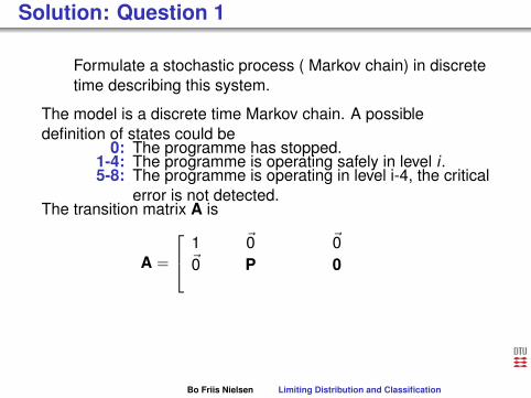
Solution: Question 1
Formulate a stochastic process ( Markov chain) in discretetime describing this system.
The model is a discrete time Markov chain. A possibledefinition of states could be
0: The programme has stopped.1-4: The programme is operating safely in level i .5-8: The programme is operating in level i-4, the critical
error is not detected.The transition matrix A is
A =
1 ~0 ~0~0 P 0
~r Diag(qi)P Diag(Si)P
Bo Friis Nielsen Limiting Distribution and Classification

Solution: Question 1
Formulate a stochastic process ( Markov chain) in discretetime describing this system.
The model is a discrete time Markov chain. A possibledefinition of states could be
0: The programme has stopped.1-4: The programme is operating safely in level i .5-8: The programme is operating in level i-4, the critical
error is not detected.The transition matrix A is
A =
1 ~0 ~0~0 P 0~r
Diag(qi)P Diag(Si)P
Bo Friis Nielsen Limiting Distribution and Classification

Solution: Question 1
Formulate a stochastic process ( Markov chain) in discretetime describing this system.
The model is a discrete time Markov chain. A possibledefinition of states could be
0: The programme has stopped.1-4: The programme is operating safely in level i .5-8: The programme is operating in level i-4, the critical
error is not detected.The transition matrix A is
A =
1 ~0 ~0~0 P 0~r Diag(qi)P
Diag(Si)P
Bo Friis Nielsen Limiting Distribution and Classification
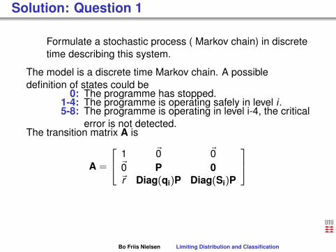
Solution: Question 1
Formulate a stochastic process ( Markov chain) in discretetime describing this system.
The model is a discrete time Markov chain. A possibledefinition of states could be
0: The programme has stopped.1-4: The programme is operating safely in level i .5-8: The programme is operating in level i-4, the critical
error is not detected.The transition matrix A is
A =
1 ~0 ~0~0 P 0~r Diag(qi)P Diag(Si)P
Bo Friis Nielsen Limiting Distribution and Classification
Question 1 - continued
The model is a discrete time Markov chain. Where P = {pij}
~r =
r1r2r3r4
Diag(Si) =
S1 0 0 00 S2 0 00 0 S3 00 0 0 S4
Si = 1− ri − qi
Diag(qi) =
q1 0 0 00 q2 0 00 0 q3 00 0 0 q4
Bo Friis Nielsen Limiting Distribution and Classification

Question 1 - continued
The model is a discrete time Markov chain.
Where P = {pij}
~r =
r1r2r3r4
Diag(Si) =
S1 0 0 00 S2 0 00 0 S3 00 0 0 S4
Si = 1− ri − qi
Diag(qi) =
q1 0 0 00 q2 0 00 0 q3 00 0 0 q4
Bo Friis Nielsen Limiting Distribution and Classification

Question 1 - continued
The model is a discrete time Markov chain. Where P = {pij}
~r =
r1r2r3r4
Diag(Si) =
S1 0 0 00 S2 0 00 0 S3 00 0 0 S4
Si = 1− ri − qi
Diag(qi) =
q1 0 0 00 q2 0 00 0 q3 00 0 0 q4
Bo Friis Nielsen Limiting Distribution and Classification

Question 1 - continued
The model is a discrete time Markov chain. Where P = {pij}
~r =
r1r2r3r4
Diag(Si) =
S1 0 0 00 S2 0 00 0 S3 00 0 0 S4
Si = 1− ri − qi
Diag(qi) =
q1 0 0 00 q2 0 00 0 q3 00 0 0 q4
Bo Friis Nielsen Limiting Distribution and Classification
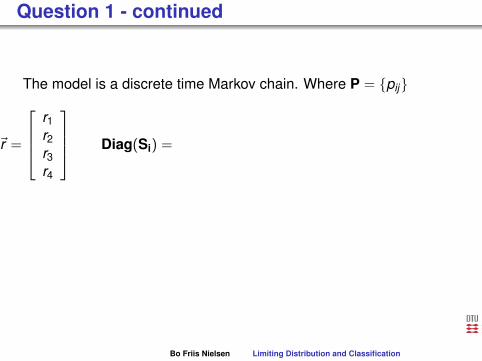
Question 1 - continued
The model is a discrete time Markov chain. Where P = {pij}
~r =
r1r2r3r4
Diag(Si) =
S1 0 0 00 S2 0 00 0 S3 00 0 0 S4
Si = 1− ri − qi
Diag(qi) =
q1 0 0 00 q2 0 00 0 q3 00 0 0 q4
Bo Friis Nielsen Limiting Distribution and Classification

Question 1 - continued
The model is a discrete time Markov chain. Where P = {pij}
~r =
r1r2r3r4
Diag(Si) =
S1 0 0 00 S2 0 00 0 S3 00 0 0 S4
Si = 1− ri − qi
Diag(qi) =
q1 0 0 00 q2 0 00 0 q3 00 0 0 q4
Bo Friis Nielsen Limiting Distribution and Classification

Question 1 - continued
The model is a discrete time Markov chain. Where P = {pij}
~r =
r1r2r3r4
Diag(Si) =
S1 0 0 00 S2 0 00 0 S3 00 0 0 S4
Si = 1− ri − qi
Diag(qi) =
q1 0 0 00 q2 0 00 0 q3 00 0 0 q4
Bo Friis Nielsen Limiting Distribution and Classification

Question 1 - continued
The model is a discrete time Markov chain. Where P = {pij}
~r =
r1r2r3r4
Diag(Si) =
S1 0 0 00 S2 0 00 0 S3 00 0 0 S4
Si = 1− ri − qi
Diag(qi)
=
q1 0 0 00 q2 0 00 0 q3 00 0 0 q4
Bo Friis Nielsen Limiting Distribution and Classification

Question 1 - continued
The model is a discrete time Markov chain. Where P = {pij}
~r =
r1r2r3r4
Diag(Si) =
S1 0 0 00 S2 0 00 0 S3 00 0 0 S4
Si = 1− ri − qi
Diag(qi) =
q1 0 0 00 q2 0 00 0 q3 00 0 0 q4
Bo Friis Nielsen Limiting Distribution and Classification

Question 1 - continued
Or without matrix notation:
A =
1 0 0 0 0 0 0 0 00 p11 p12 p13 p14 0 0 0 00 p21 p22 p23 p24 0 0 0 00 p31 p32 p33 p34 0 0 0 00 p41 p42 p43 p44 0 0 0 0r1 q1p11 q1p12 q1p13 q1p14 S1p11 S1p12 S1p13 S1p14r2 q2p21 q2p22 q2p23 q2p24 S2p21 S2p22 S2p23 S2p24r3 q3p31 q3p32 q3p33 q3p34 S3p31 S3p32 S3p33 S3p34r4 q4p41 q4p42 q4p43 q4p44 S4p41 S4p42 S4p43 S4p44
Bo Friis Nielsen Limiting Distribution and Classification

Question 1 - continued
Or without matrix notation:
A
=
1 0 0 0 0 0 0 0 00 p11 p12 p13 p14 0 0 0 00 p21 p22 p23 p24 0 0 0 00 p31 p32 p33 p34 0 0 0 00 p41 p42 p43 p44 0 0 0 0r1 q1p11 q1p12 q1p13 q1p14 S1p11 S1p12 S1p13 S1p14r2 q2p21 q2p22 q2p23 q2p24 S2p21 S2p22 S2p23 S2p24r3 q3p31 q3p32 q3p33 q3p34 S3p31 S3p32 S3p33 S3p34r4 q4p41 q4p42 q4p43 q4p44 S4p41 S4p42 S4p43 S4p44
Bo Friis Nielsen Limiting Distribution and Classification

Question 1 - continued
Or without matrix notation:
A =
1 0 0 0 0 0 0 0 0
0 p11 p12 p13 p14 0 0 0 00 p21 p22 p23 p24 0 0 0 00 p31 p32 p33 p34 0 0 0 00 p41 p42 p43 p44 0 0 0 0r1 q1p11 q1p12 q1p13 q1p14 S1p11 S1p12 S1p13 S1p14r2 q2p21 q2p22 q2p23 q2p24 S2p21 S2p22 S2p23 S2p24r3 q3p31 q3p32 q3p33 q3p34 S3p31 S3p32 S3p33 S3p34r4 q4p41 q4p42 q4p43 q4p44 S4p41 S4p42 S4p43 S4p44
Bo Friis Nielsen Limiting Distribution and Classification
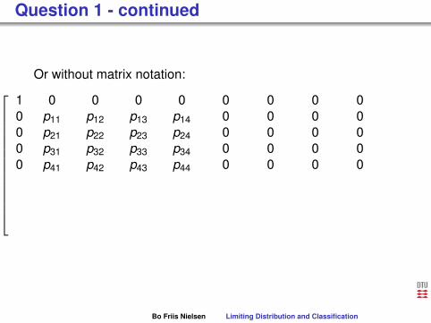
Question 1 - continued
Or without matrix notation:
A =
1 0 0 0 0 0 0 0 00 p11 p12 p13 p14 0 0 0 00 p21 p22 p23 p24 0 0 0 00 p31 p32 p33 p34 0 0 0 00 p41 p42 p43 p44 0 0 0 0
r1 q1p11 q1p12 q1p13 q1p14 S1p11 S1p12 S1p13 S1p14r2 q2p21 q2p22 q2p23 q2p24 S2p21 S2p22 S2p23 S2p24r3 q3p31 q3p32 q3p33 q3p34 S3p31 S3p32 S3p33 S3p34r4 q4p41 q4p42 q4p43 q4p44 S4p41 S4p42 S4p43 S4p44
Bo Friis Nielsen Limiting Distribution and Classification

Question 1 - continued
Or without matrix notation:
A =
1 0 0 0 0 0 0 0 00 p11 p12 p13 p14 0 0 0 00 p21 p22 p23 p24 0 0 0 00 p31 p32 p33 p34 0 0 0 00 p41 p42 p43 p44 0 0 0 0r1 q1p11 q1p12 q1p13 q1p14 S1p11 S1p12 S1p13 S1p14r2 q2p21 q2p22 q2p23 q2p24 S2p21 S2p22 S2p23 S2p24r3 q3p31 q3p32 q3p33 q3p34 S3p31 S3p32 S3p33 S3p34r4 q4p41 q4p42 q4p43 q4p44 S4p41 S4p42 S4p43 S4p44
Bo Friis Nielsen Limiting Distribution and Classification

Solution question 2
Characterise the states in the Markov chain.
With reasonable assumptions on P (i.e. irreducible) we getState 0 Absorbing1 Positive recurrent2 Positive recurrent3 Positive recurrent4 Positive recurrent5 Transient6 Transient7 Transient8 Transient
Bo Friis Nielsen Limiting Distribution and Classification

Solution question 2
Characterise the states in the Markov chain.
With reasonable assumptions on P (i.e. irreducible) we get
State 0 Absorbing1 Positive recurrent2 Positive recurrent3 Positive recurrent4 Positive recurrent5 Transient6 Transient7 Transient8 Transient
Bo Friis Nielsen Limiting Distribution and Classification

Solution question 2
Characterise the states in the Markov chain.
With reasonable assumptions on P (i.e. irreducible) we getState 0
Absorbing1 Positive recurrent2 Positive recurrent3 Positive recurrent4 Positive recurrent5 Transient6 Transient7 Transient8 Transient
Bo Friis Nielsen Limiting Distribution and Classification
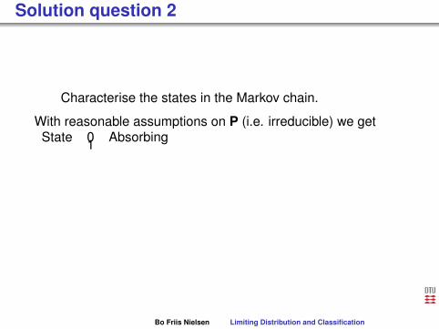
Solution question 2
Characterise the states in the Markov chain.
With reasonable assumptions on P (i.e. irreducible) we getState 0 Absorbing1
Positive recurrent2 Positive recurrent3 Positive recurrent4 Positive recurrent5 Transient6 Transient7 Transient8 Transient
Bo Friis Nielsen Limiting Distribution and Classification

Solution question 2
Characterise the states in the Markov chain.
With reasonable assumptions on P (i.e. irreducible) we getState 0 Absorbing1 Positive recurrent2
Positive recurrent3 Positive recurrent4 Positive recurrent5 Transient6 Transient7 Transient8 Transient
Bo Friis Nielsen Limiting Distribution and Classification
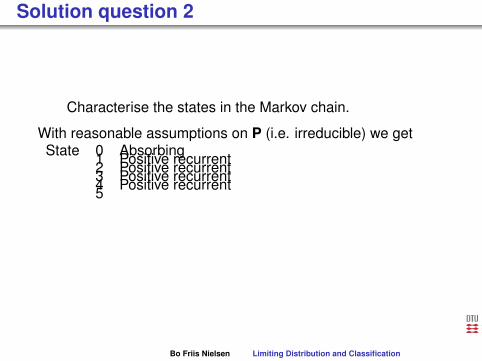
Solution question 2
Characterise the states in the Markov chain.
With reasonable assumptions on P (i.e. irreducible) we getState 0 Absorbing1 Positive recurrent2 Positive recurrent3 Positive recurrent4 Positive recurrent5
Transient6 Transient7 Transient8 Transient
Bo Friis Nielsen Limiting Distribution and Classification

Solution question 2
Characterise the states in the Markov chain.
With reasonable assumptions on P (i.e. irreducible) we getState 0 Absorbing1 Positive recurrent2 Positive recurrent3 Positive recurrent4 Positive recurrent5 Transient6 Transient7 Transient8 Transient
Bo Friis Nielsen Limiting Distribution and Classification

Solution question 3
We now consider the case where the stability of the system hasbeen assured, i.e. the error has been found and corrected, andthe program has been running for long time without errors. Theparameters are as follows.
Pi,i+1 = 0.6 i = 1,2,3 Pi,i−1 = 0.2 i = 2,3,4Pi,j = 0 |i − j | > 1 qi = 10−3i ri = 10−3i−5
Characterise the stochastic proces, that describes thestable system.
The system becomes stable by reaching one of the states 1-4.The process is ergodic from then on. The procces is areversible ergodic Markov chain in discrete time.
Bo Friis Nielsen Limiting Distribution and Classification

Solution question 3
We now consider the case where the stability of the system hasbeen assured, i.e. the error has been found and corrected, andthe program has been running for long time without errors. Theparameters are as follows.Pi,i+1 = 0.6 i = 1,2,3 Pi,i−1 = 0.2 i = 2,3,4Pi,j = 0 |i − j | > 1 qi = 10−3i ri = 10−3i−5
Characterise the stochastic proces, that describes thestable system.
The system becomes stable by reaching one of the states 1-4.
The process is ergodic from then on. The procces is areversible ergodic Markov chain in discrete time.
Bo Friis Nielsen Limiting Distribution and Classification

Solution question 3
We now consider the case where the stability of the system hasbeen assured, i.e. the error has been found and corrected, andthe program has been running for long time without errors. Theparameters are as follows.Pi,i+1 = 0.6 i = 1,2,3 Pi,i−1 = 0.2 i = 2,3,4Pi,j = 0 |i − j | > 1 qi = 10−3i ri = 10−3i−5
Characterise the stochastic proces, that describes thestable system.
The system becomes stable by reaching one of the states 1-4.The process is ergodic from then on.
The procces is areversible ergodic Markov chain in discrete time.
Bo Friis Nielsen Limiting Distribution and Classification

Solution question 3
We now consider the case where the stability of the system hasbeen assured, i.e. the error has been found and corrected, andthe program has been running for long time without errors. Theparameters are as follows.Pi,i+1 = 0.6 i = 1,2,3 Pi,i−1 = 0.2 i = 2,3,4Pi,j = 0 |i − j | > 1 qi = 10−3i ri = 10−3i−5
Characterise the stochastic proces, that describes thestable system.
The system becomes stable by reaching one of the states 1-4.The process is ergodic from then on. The procces is areversible ergodic Markov chain in discrete time.
Bo Friis Nielsen Limiting Distribution and Classification

Solution question 4
For what fraction of time will the system be in level 1.
We obtain the following steady state equations
πi = 3i−1π1
4∑i=1
3i−1π1 = 1⇔ 40π1 = 1
π1 =140
The sum∑4
i=1 3i−1 can be obtained by using∑4i=1 3i−1 = 1−34
1−3 = 40.
4∑i=1
3i−1π1 = 1⇔ 1− 34
1− 3π1 = 1
Bo Friis Nielsen Limiting Distribution and Classification

Solution question 4
For what fraction of time will the system be in level 1.We obtain the following steady state equations
πi = 3i−1π1
4∑i=1
3i−1π1 = 1⇔ 40π1 = 1
π1 =140
The sum∑4
i=1 3i−1 can be obtained by using∑4i=1 3i−1 = 1−34
1−3 = 40.
4∑i=1
3i−1π1 = 1⇔ 1− 34
1− 3π1 = 1
Bo Friis Nielsen Limiting Distribution and Classification
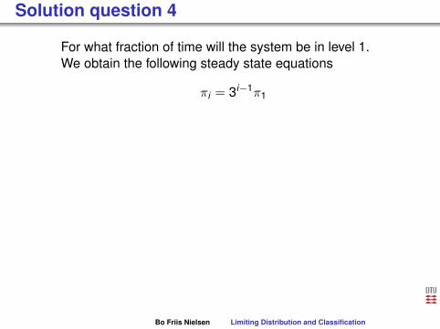
Solution question 4
For what fraction of time will the system be in level 1.We obtain the following steady state equations
πi = 3i−1π1
4∑i=1
3i−1π1 = 1
⇔ 40π1 = 1
π1 =140
The sum∑4
i=1 3i−1 can be obtained by using∑4i=1 3i−1 = 1−34
1−3 = 40.
4∑i=1
3i−1π1 = 1⇔ 1− 34
1− 3π1 = 1
Bo Friis Nielsen Limiting Distribution and Classification

Solution question 4
For what fraction of time will the system be in level 1.We obtain the following steady state equations
πi = 3i−1π1
4∑i=1
3i−1π1 = 1⇔ 40π1 = 1
π1 =140
The sum∑4
i=1 3i−1 can be obtained by using∑4i=1 3i−1 = 1−34
1−3 = 40.
4∑i=1
3i−1π1 = 1⇔ 1− 34
1− 3π1 = 1
Bo Friis Nielsen Limiting Distribution and Classification

Solution question 4
For what fraction of time will the system be in level 1.We obtain the following steady state equations
πi = 3i−1π1
4∑i=1
3i−1π1 = 1⇔ 40π1 = 1
π1 =140
The sum∑4
i=1 3i−1 can be obtained by using∑4i=1 3i−1 = 1−34
1−3 = 40.
4∑i=1
3i−1π1 = 1⇔ 1− 34
1− 3π1 = 1
Bo Friis Nielsen Limiting Distribution and Classification
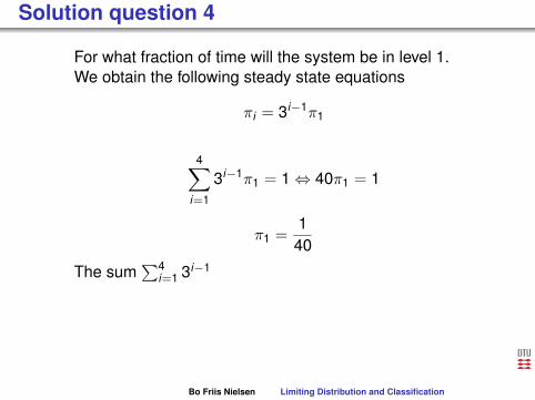
Solution question 4
For what fraction of time will the system be in level 1.We obtain the following steady state equations
πi = 3i−1π1
4∑i=1
3i−1π1 = 1⇔ 40π1 = 1
π1 =140
The sum∑4
i=1 3i−1
can be obtained by using∑4i=1 3i−1 = 1−34
1−3 = 40.
4∑i=1
3i−1π1 = 1⇔ 1− 34
1− 3π1 = 1
Bo Friis Nielsen Limiting Distribution and Classification
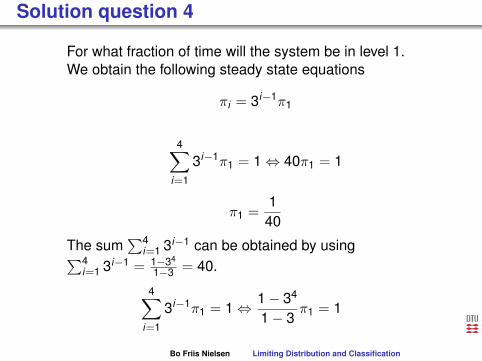
Solution question 4
For what fraction of time will the system be in level 1.We obtain the following steady state equations
πi = 3i−1π1
4∑i=1
3i−1π1 = 1⇔ 40π1 = 1
π1 =140
The sum∑4
i=1 3i−1 can be obtained by using∑4i=1 3i−1 = 1−34
1−3 = 40.
4∑i=1
3i−1π1 = 1⇔ 1− 34
1− 3π1 = 1
Bo Friis Nielsen Limiting Distribution and Classification