.... =,

.NASATechnical

Paper2989 ......

/

-]

i

-=_ =

w

5 9__/7 /6_

Discrete-VortexModel for theSymmetric-VortexFlow on Cones

Thomas G. Gainer

1 (" = ,Tt'; :,YH_tc-TP, I(-V_'_iCTc X r--LOW dkl CONES (NA__A)

i 20 0 L.SCL OIA Uncl as

-- HI/O2 02o47_3

https://ntrs.nasa.gov/search.jsp?R=19900011630 2018-07-28T06:27:36+00:00Z

.......... - . .

_ _ m

=

n

NASATechnical

Paper2989

1990

National Aeronautics andSpace Administration

Office of ManagementScientific and TechnicalInformation Division

Discrete-VortexModel for theSymmetric-VortexFlow on Cones

Thomas G. Gainer

Langley Research Center

Hampton, Virginia

Summary

A relatively simple but accurate potential-flow

model has been developed for studying the

symmetric-vortex flow on cones. The model is a mod-

ified version of the model first developed by Bryson,

in which discrete vortices and straight-line feeding

sheets were used to represent the flow field. It dif-

fers, however, in the zero-force condition used to po-sition the vortices and determine their circulation

strengths. The Bryson model imposed the condition

that the net force on the feeding sheets and discrete

vortices must be zero. The proposed model satisfies

this zero-force condition by having the vortices move

as free vortices, at a velocity equal to the local cross-

flow velocity at their centers. When the free-vortex

assumption is made, a solution is obtained in theform of two nonlinear algebraic equations that relate

the vortex-center coordinates and vortex strengths

to the cone angle and angle of attack. The vortex-center locations calculated using the model are in

good agreement with experimental values. The conenormal forces and center locations are in good agree-

ment with the vortex cloud method of calculating

symmetric flow fields.

Introduction

The symmetric-vortex flow on cones has beenstudied in several investigations in connection with

the high-angle-of-attack performance of aircraft and

missiles. Designers would like to use the lift pro-

duced by these flows to improve maneuvering ca-

pability, but they also want to understand and be

able to predict adverse flow patterns, such as vortex

asymmetry, that can occur. Vortex asymmetries usu-

ally occur at moderate to high angles of attack and

can cause serious stability and control problems. A

thorough knowledge of the symmetric-vortex flowfield could lead to a better understanding of why and

under what conditions these asymmetries occur.

The previous analytical studies of conical vor-tex flow have included Navier-Stokes solutions, ob-

tained mainly at supersonic speeds (refs. 1 to 3), and

potential-flow solutions, obtained using free-sheet

methods (refs. 4 to 7). More recently, a vortex cloud

method (refs. 8 and 9) has been developed that allowsvortex flow characteristics to be determined for cones

as well as general forebody shapes. These methods,

however, involve fairly complicated time-stepping or

iteration procedures, and the results available in the

literature cover only a limited number of cone angles

and angles of attack. The effects of the different pa-

rameters governing conical vortex flow have not been

clearly defined.

This report describes a relatively simple discrete-

vortex model for studying the vortex flow on cones.

The model is based on the Bryson model described in

references 10 and 11, but uses a different zero-force

condition than that used by Bryson to locate thevortices and determine their circulation strengths.

Bryson imposed the condition that there be zero net

force on a system consisting of primary vortices and

straight-line feeding sheets. In the present model,

this zero-force condition is satisfied by having the

vortices move as free vortices, that is, at velocities

equal to the local flow velocities at their centers.

The assumptions of a free vortex and conicalflow enable a solution to be obtained in the form

of two nonlinear algebraic equations that relate vor-

tex position, vortex strength, and the parameter

tan c_/tan_. Together with information about the

separation point, these relationships can be used to

obtain a solution for a given cone angle and angle ofattack.

The vortex centers calculated using the present

method are shown to be in good agreement with

the experimental data obtained at incompressiblelaminar-flow conditions in reference 12. When the

measured separation points are used, the method

gives an accurate prediction of the travel of the vortex

centers as the cone goes through an angle-of-attack

range. The vortex-center locations and normal forces

predicted using the method also agree with those pre-

dicted using the vortex cloud method of references 8and 9 for the same circulation strength.

Symbols

a

all, bll

a12, b12

a21, b21

X-axis influence coefficient

(symmetric-vortex alignment)

X- and Y-axis influence coeffi-

cients, respectively, that express

influence of image of vortex 1 onconditions at center of vortex 1 for

asymmetric-vortex alignment (see

fig. B1)

X- and Y-axis influence coefficients,

respectively, that express influenceof vortex 2 and its image on con-

ditions at vortex 1 for asymmetric-

vortex alignment (see fig. B1)

X- and Y-axis influence coefficients,

respectively, that express influence

of vortex 1 and its image on con-

ditions at vortex 2 for asymmetric-

vortex alignment (see fig. B1)

a22, b22

Ck

Ck,avail

Ck,req

Cy

CN

D

dp

F

FF.S.

i

k

L

MV

r

TO

S

t

U

X- and Y-axis influence coeffi-

cients, respectively, that expressinfluence of image of vortex 2 onconditions at center of vortex 2 for

asymmetric-vortex alignment (seefig. B1)

Y-axis influence coefficient

(symmetric-vortex alignment)

nondimensionai vortex strength,F

2nroUccsin a

nondimensional vortex strengthmade available for vortex formation

by boundary-layer separation oncone

nondimensional vortex strengthrequired to meet the zero-forcecondition

Normal force

normal-force coefficient, (1/2)pU2 S

local normal-force coefficient,measured in X-Y plane at agiven z-station along cone axis,Local normal force

(1/2)pU2 D

diameter of cone base

differential pressure across a feedingsheet

force exerted on vortex system bybody at a given cross section

pressure force on feeding sheet

local normal force

Kutta-Joukowski force acting atvortex center

unit vector along imaginary axis

vorticity reduction factor

length of cone

momentum of vortex pair

radial distance in crossflow plane,

radius of cone cross section

base area of cone

time

X-axis component of velocity,nondimensionalized with respectto U_ sin a, that results from free-

stream flow around cone at a givencross section

V_

V

v

w

x

x !

Y

yi

z

F

I_avail

P

¢

¢,

velocity at edge of boundary layerat a separation point on cone

free-stream velocity

= _z, X-axis component of velocityat a point in flow field, nondimen-sionalized with respect to U_ sin a

Y-axis component of velocity,nondimensionalized with respectto Uc¢ sin a, that results from free-stream flow around cone at a givencross section

induced velocity at vortex center,Uk + ivk

= _,, Y-axis component of velocity

at a point in flow field, nondimen-sionalized with respect to Uc¢ sin a

complex potential, ¢ + i¢

X-axis coordinate (see fig. 1)

X/?" o

Y-axis coordinate (see fig. 1)

= y/ro

Z-axis coordinate (see fig. 1)

cone angle of attack

circulation, positive clockwise infirst (+x, +y) quadrant of X-Yplane

circulation made available for

vortex formation by boundary-layerseparation taking place on cone

cone semi-apex angle

-- x + iy, complex coordinate of apoint in flow field

complex coordinate of origin offeeding sheet (see fig. A1)

= tan-l(z_), angle measured frompositive X-axis to a point in flowfield

fluid density

velocity potential

angular distance to separation pointon cone at a given cross section,measured from negative X-axis (seefig. 1)

¢ stream function

Subscripts and superscripts:

k primary vortex index

(-) complex conjugate

1 refers to conditions at center of

vortex 1 (see fig. BI/

2 refers to conditions at center of

vortex 2 (see fig. B1)

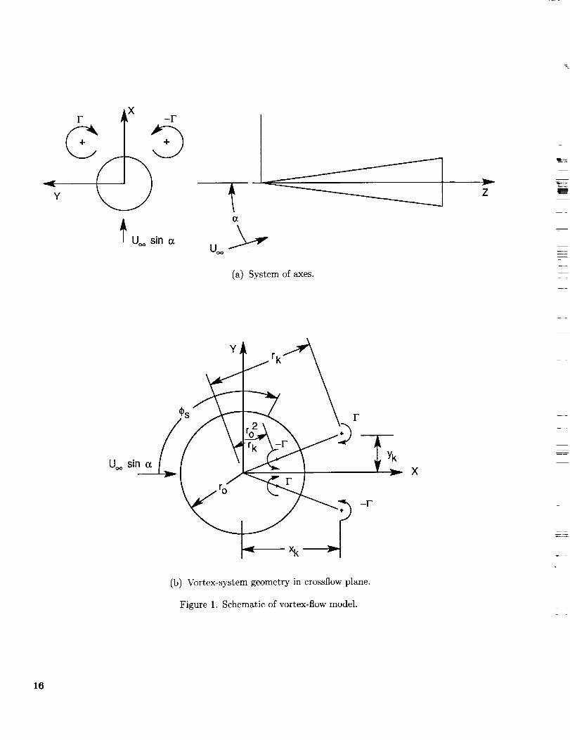
Mathematical Development

Basic Flow Model

The model used (see fig. 1/ is the two-dimensional,discrete-vortex model that is described in refer-

ence 13 and used by a number of investigators, butwith a source term added to simulate conical flow.

The model assumes incompressible potential flow.

The flow at each cross section is represented by two

primary vortices placed at the positions x k and +Ykwith image vortices placed inside the cone at the po-

sitions shown in figure 1 to satisfy the tangent-flow

boundary condition on the surface. The added source

term has a strength that varies with the distance z

along the cone axis and simulates the velocities thatoccur normal to the surface at each cross section in

conical flow. The complex potential for this systemis

+2"_ir [ln(_-_k)-ln( _-r2_¢k]

- In(_- _k) +In _--E]J

- roU_ cos _ tan _ In _ (1)

The first term on the right-hand side in equa-

tion (1) is the complex potential for the free-stream

flow around the cross section; the second through

fifth terms are those for the primary vortices andtheir images; the last term is the source term addedfor conical flow. This source term assumes the flow

is purely conical, that is, all flow quantities are con-

stant along rays emanating from the cone apex. Thisterm does not account for the end effects that result

from the cone having a finite length. (For examples

of more complex representations that do account for

end effects, see ref. 14. /

The real part of equation (1 / gives the velocity

potential

( )¢=U_sina 1+x2+y2 x

F

27rroUoo sin

- tan-1 _x-----k)

_tan-t(Y+Y_______k_+tan -1 ___

-- roUo_ cos _ tan 6 In # + y2 (21

The imaginary part of equation (1) gives thestream function

( )¢=Uoosina 1 x 2+y2 Y

+ In - 2 + (v - vk)2

-- In V/(x - Xk) 2 + (y + yk) 2

-- roUoc cos a tan _ tan 8 (3)

The nondimensional velocity in the x direction,

written in terms of x _ and yl coordinates is given by

u_---r

+

+

xl2+ y,2 (zt2 + y,2)2]

F

27rroU_ sin

r2 i\ 2 r2 i'_2+(y'+

- + +

r 2 I

---- 2

tan 6 cos/9(4)+ tan a/_

yl2V_, +

This velocity can be written as

tan 6 cos 0u = u + aCE+ -- (5)

tall ol ¢X/2 + yt2

where a is an X-axis influence coefficient equal tor in

the sum of the terms multiplied by 27rroUe_sine

equation (4).

The velocity in the y-direction is given by

xly I Fv= -2 +

(x,2 + y,212 2rroUccsin_

+

2 2 r2 t 2

+(,'-

+(¢

tan 6 sin 0+

tan _ V_ + yt2

x/ _ r2 I

(6)

This velocity can be written as

tan 6 sin 0= (7)v V+bC k+tan_/-a

yt2Vz, +

where b is a Y-axis-oriented influence coefficient

equal to the sum of the terms multiplied byr in equation (6).

2rcroUo_ sin c_

Solution for Conical Flow

The basic flow problem can be solved if the lo-

cations and circulation strengths of the primary vor-

tices are known. Equation (2) defines a velocity po-

tential 05 that is a function of x and y and satisfiesthe Laplace equation and the boundary conditions

of the problem. The Laplace equation is automat-ically satisfied because each of the singularities in-

volved satisfies the Laplace equation. One bound-

ary condition--that the flow must be tangent to the

body at the surface_is satisfied by the image systemused. The other boundary condition--that the flow

velocity at infinity must be equal to the free-stream

velocity--is satisfied because the velocity induced by

each of the singularities varies inversely withthe dis-

tance from the singularity.

Once this velocity potential is defined, the veloci-

ties at different points in the potential flow field and

the forces on the body can be determined. The prob-

lem then becomes one of determining the locationsand circulation strengths of the vortex centers for

different cone angles and angles of attack. These lo-

cations and strengths are usually determined by im-

posing a zero-force condition to constrain the motion

of the primary vortices.

Zero-Force Condition

The zero-force condition imposed in the present

method is that the primary vortices move as free

vortices, that is, at a velocity equal to the localfluid velocity of the vortex centers. This condition

is expressed mathematically by

d_kvk"= d-T (8)

This condition is a departure from the zero-force

condition used by Bryson and others (e.g., see refs. 7

and 10), for which the force on a feeding sheet that

extends into the vortex is balanced out by an equaland opposite force at the vortex center; thus, there

is no net force on the vortex system. However, the

use of equation (8) is justified in appendix A.

L

_qE:_

Conical Flow Assumptions

Equation (8) relates the induced velocity at the

vortex center to the absolute velocity _t of the cen-ter relative to the axis-system origin. This absolute

velocity can be expressed in terms of cone semi-apex

angle and angle of attack by assuming conical flow

and making use of the impulsive-flow analogy. Ac-

cording to the impulsive-flow analogy (e.g., ref. 15),

the flow at a given cross section of the cone is equiva-lent to that about a two-dimensional cylinder whose

radius is expanding with time, where time in the two-dimensional plane is related to the distance along the

axis of the three-dimensional cone by

zt = (9)

Voo cos a

If the flow is assumed to be conical, the movement ofthe vortex center is known. The center moves radially

away from the cone axis as either time (in the two-

dimensional plane) or distance z (along the three-dimensional body) increases. Therefore, the velocity

of the vortex center at a given cross section must

point in the radial direction and have a magnitude of

drk (drk (10)dtt - Uoccos a \ dz ]

Now the derivative with respect to z can be

written as

dr k _ (drk_ Idro_ = (drk_tan 6 (11)dz \ dro ] \ dz ] \ dro ]

Since, for conical flow, the nondimensional distanceto the vortex center remains constant for a given cone

angle and angle of attack,

drk ( rk ) (12)-- _o tan6 Uoccosa

The velocity of the vortex center, nondimensionalized

with respect to Ucc sin a, can therefore be written as

1 (drk_= (rk) tan_ (13)Uoc sin a \ dt ] -_o _an a

Equations for Ck and tan a/tan 6

In terms of nondimensionalized X- and Y-axis ve-

locity components, the zero-force condition (eq. (8))becomes

Uk+akCk+tan6 (c°sOk_ = (rk) tan_t_---Gt_--f7Go] 7o _ co_0_ (14)

Vk +bkCk + _ trk/ro] _ t-'_"_asin0k

(For an extension of the zero-force equations

(eqs. (14) and (15)) to asymmetric-vortex align-

ments, see appendix B.) Here, Ck,req is a requirednondimensional vortex strength--it is needed to meet

the zero-force condition for a given vortex-center

location. The influence coefficients ak and bk in

equations (14) and (15) omit the respective terms

Y'-Yk , (see eq. (4)) and -(x'-x_)v t 2 2(x'-x_)_+(V-Yk)_ (x-_k) +(¢-_)

(see eq. (6)) since, in potential flow calculations, itcan be assumed that a discrete straight-line vortex

has no influence on itself. (See ref. 16.)

Combining the terms containing tan a/tan 6 and

dividing equation (15) by equation (14) gives

V k + bkCk

V k q- akC k----tan0 k (16)

from which the circulation required to meet the zero-force condition can be determined as

- (Uk tan Ok - Vk) (17)Ck,req = (ak tanOk -- bk)

Since the factors defining the nondimensional vortex

strength in equation (17)--Uk, Vk,ak, and bk--are

functions of xk and Yk only, this nondimensional

strength is uniquely defined by the vortex-centerlocation.

The value of tan a/tan 6 corresponding to a givenvortex-center location and nondimensional vortex

strength can be determined from either equation (14)

or (15) as follows:

1 ) cos Oktana (rk/r°)- rk---]Go

tan

(Vk + bkCk)(18)

Equations (17) and (18) form the basis of the

present method; they provide two equations in terms

of the known parameter tan a/tan 6 and the three un-

known parameters _Xk, Yk, and Ck,req. A third equa-tion that is available for solving the problem is an

equation for the vortex strength. The nondimen-sional vortex strength given by equation (17) is that

required to meet the zero-force condition, but justwhat value this strength achieves for a given value of

tan a/tan _ depends on how much circulation is madeavailable for vortex formation by the boundary-layer

separation that is taking place on the cone. Thisavailable circulation can be determined from the rate

q_

at which circulation is generated at the separation

points on the cone.

Determination of Available Circulation

If the location of the separation point on the cone

is known, having been either measured or calculated

using a boundary-layer-separation criterion such as

that employed in the vortex cloud program of refer-

ences 8 and 9, then the rate at which circulation is

generated can be approximated by the relationship:

where Ue is the edge velocity at the separation point

(it includes the velocities induced by the vortices).The k factor is a vorticity modification factor that

accounts for the fact that, in general, not all the

vorticity generated by the boundary-layer separation

is entrained into the primary vortices. A k factor of

0.6 is usually assumed. (See ref. 8.)

Since, for conical flow, F varies linearly with t,

dr.,,_il = r_,,_il (20)dt t

By using equation (9), equation (19) can be writtenas

Ck,av_l = -_r n a tan 5

which is the nondimensional vortex strength available

for a given value of tan a/tan 5.

Calculation of Normal-Force Coefficients

Once the nondimensional vortex strengths and

locations of the vortex centers have been determined,the normal forces on the cone can be calculated from

the equations derived in appendix C. The equation

used for calculating the local normal-force coefficient

at a given cross section is

The equation for the normal-force coefficient for the

complete cone is

° s n0 ]s oo o o(23)

Results and Discussion

that is, at a velocity equal to the local crossflow ve-

locity at their centers. The vortex-center positions

and circulation strengths needed to meet this condi-

tion for different cone angles and angles of attack are

shown in figure 2. Figure 2 shows contours, obtained

by iteration from equations (17) and (18), of con-

stant circulation strength (solid lines) and the values

of tan a/tan 5 (dashed lines); these contours are plot-

ted as functions of the coordinates of the primary

vortex center, x_ and ylk. Figure 2 can be used intwo ways. If the available circulation strength has

been determined for a given cone angle and angle of

attack--either by a boundary-layer calculation or by

experiment--the contours in figure 2 can be used tolocate the coordinates of the vortex center. If, on

the other hand, the vortex-center location has been

measured experimentally, these contours can be used

to approximate the circulation strengths of the vor-

tices. In either case, the complete potential-flow field

can be mapped out, and forces on the body can bedetermined.

The curves in figure 2 show a limit to vortex-center travel. The vortex centers would not be ex-

pected to go beyond the curve for which tan a/tan 5

is infinite (a cone angle of attack of 90°). The curve

that defines this limit is the so-called FSppl curve.

(See refs. 13 and 17.) The FSppl curve gives thelocations of the vortex centers for which the veloc-

ity Vk* at the center is zero for a constant-diametercylinder in two-dimensional flow. It can be shown

that this condition corresponds to having the denom-

inators in the equations for tana/tan5 (eqs. (18))equal to zero, which would produce an infinite value

of tan a/tan 5. The FSppl curve, therefore, definesthe limit of vortex-center travel for conical flow.

Comparison of Calculated Center

Locations With Experiment

Figure 3 shows measured vortex-center locations

from reference 12 superimposed on the constant C kand tan a/tan 5 curves of figure 2. The experimental

results were obtained in a water tunnel at a Reynolds

number (ba._,ed on cone length i 0fabout 2.7 x 104.

(The boundary layers for this condition were de-

scribed in ref. 12 as being steady and laminar.) The

results are shown for cone semi-apex angles of 7.5 °

and 12.5 ° in figures 3(a) and 3(b), respectively. The

values of tan a/tan_ for individual data points are

indicated in the figures. These results show that asthe angle of attack is increased, the vortex center

Vortex-Center Locations as a Function of moves-upward, toward curves for higher values of

Ck and tana/tan5 Ck, and to the right, toward curves for higher val-

In the present method, the primary vortices are ues of tan a/tan 5. For both cones, the measured

kept force-free by having them move as free vortices, vortex-center location for a given value of tan a/tan 5

i

6

is approximately that needed to meet the zero-force

requirement of the present method. At a value of

tan a/tan 5 of approximately 2.0, for example, theexperimental data indicate a vortex-center location

at about xk/ro = 1.16 and yk/ro = 0.33; these val-

ues are in good agreement with those needed to meetthe zero-force requirement.

The nondimensional vortex strengths of the pri-

mary vortices for the test results shown in figure 3

were not defined in reference 12; however, they were

calculated in the present investigation by using the

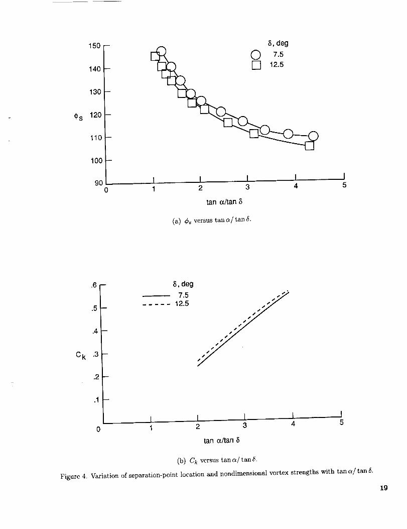
measured separation point locations given in refer-ence 12. These measured locations are shown for

the 7.5 ° and 12.5 ° cones in figure 4(a). The vortex

strengths for a given value of tan a/tan 5 and a given

separation point were determined by constructing,

for that value of tana/tanS, a curve of Yk/ro ver-

sus xk/ro similar to those shown in figures 2 and

3, and then iterating along this curve until the vor-

tex strength required to meet the zero-force condition

(eq. (17)) matched that being made available at the

separation point (eq. (21)). The nondimensional vor-

tex strengths determined by this iteration procedurefor the two cones are presented in figure 4(b), which

shows that this vortex strength was approximately a

linear function of tan a/tan 5.

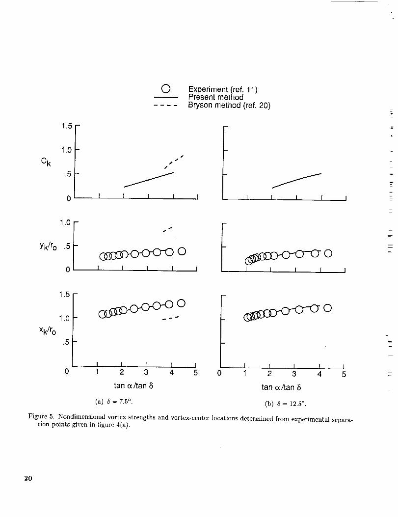
Figures 5(a) and 5(b) compare the nondimen-

sional vortex strengths given in figure 4(b) with those

determined by using the Bryson equations; these fig-

ures also compare the vortex-center locations deter-

mined by each method with the experimental-centerlocations obtained from reference 12. The vortex-

center locations calculated using the present method

are in generally good agreement with the measuredvalues over the range of values of tan a/tan 5 shown.

The predictions made with the Bryson method, on

the other hand, were not nearly as good. Because

of the relationship between Cs and tan a/tan 5 con-

tained in the Bryson zero-force equation, solutions

with the Bryson method were possible for only cer-tain segments of the curves of Cs versus tan a/tan 5

shown in figure 4(a). That is, for the 7.5 ° cone, solu-

tions were possible only for values of tan a/tan 5 be-

tween about 3.6 and 4.4; for the 12.5 ° cone, no solu-

tions were possible over the complete range of values

of tan a/tan 5 for which data were taken. The nondi-

mensional vortex strengths determined by the Bryson

method were significantly higher than those deter-

mined by the present method. The vortex-centerlocations were much farther away from the axis of

asymmetry for a given value of tan a/tan 5 than in-

dicated by either the present calculations or the ex-

perimental data.

Comparison With Vortex Cloud Results

To further verify the basic assumption of the

present method--for the cone, the vortices remain

force-free by traveling with the local crossflow

velocity--calculations made using the present

method are compared in this section with predictions

made using the vortex cloud method of references 8and 9. The vortex cloud method uses discrete vor-

tices generated at the separation points on the bodyto model the vortex wake. These discrete vortices are

assumed to travel at the local crossflow velocity and

eventually wrap up into the equivalent of the primary

vortices modeled in the present investigation. The

method uses a modified Stratford separation criterion

to determine the locations of the separation points

and assumes circulation is generated at the rate in-

dicated by equation (19) at these points. To provide

a common basis of comparison for the two methods,the calculations for both are based on the separation-

point locations and nondimensional vortex strengths

determined by the vortex cloud method.

The flow fields depicted by the two methods are

compared in figure 6. The points indicated by the

symbols are the locations of the individual vortex el-ements used in the vortex cloud method. The stream-

lines indicated in figure 6 are those calculated using

the present method. (The streamlines shown are not

actually streamlines, but rather, projections in thecrossflow plane of the paths followed by individual

particles in the three-dimensional flow.) The vortex-

center locations indicated by the two methods are in

good agreement for the three angles of attack shown.

Normal-force coefficients calculated using the

present method and the vortex cloud method are

compared in figures 7 to 9. Figure 7 shows the

variations of local normal-force coefficient cN with

distance along the body z/L for different angles of

attack. Figures 8 and 9 show the variations in to-tal normal-force coefficient with tan a/tan 5 for cone

semi-apex angles of 5° and 7.5 °, respectively. The

nondimensional vortex strengths used in obtainingthese results were those determined for the different

cone angles and angles of attack by the vortex cloud

program; these strengths are shown as a function of

tan a/tan 5 in figures 8(a) and 9(a).

Figure 7 shows generally good agreement between

the local normal-force coefficients calculated using

the two methods, based on the same nondimensional

vortex strength. The local normal-force coefficients

calculated using the vortex cloud method show some

oscillation with increasing values of z/L, particularlyfor the 5 ° cone. This oscillation is probably the result

of errors in the iteration procedure used in the vortexcloud calculations for these particular cases. The

7

present method shows a straight-line variation in cN

with z/L, which is in keeping with the conical-flowassumptions on which the method is based.

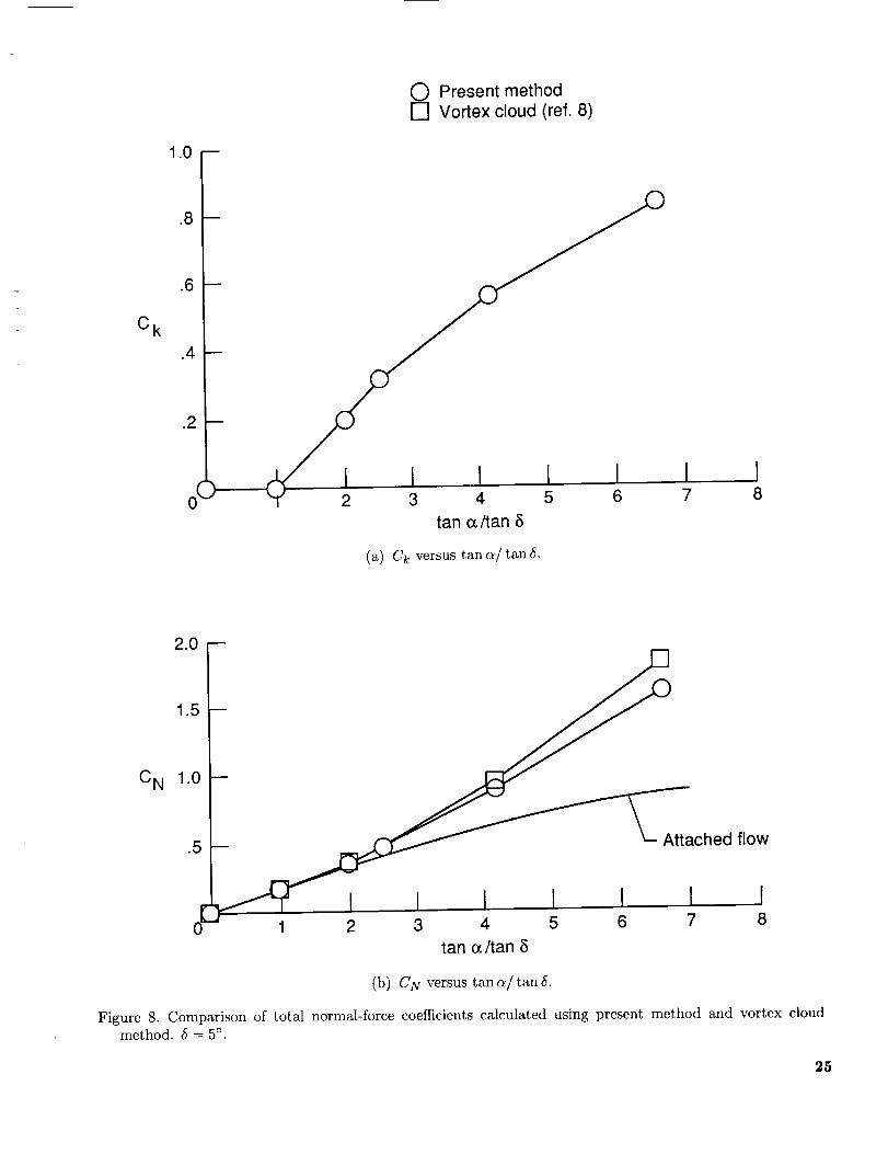
To indicate the level of the normal force produced

by vortex flow on the two cones, figures 8 and 9

show the attached-flow normal-force coefficients (thenormal-force coefficients for the cones without vor-

tex flow, as determined from slender-body theory)

and the total normal-force coefficients (the sum ofthe attached-flow and vortex-flow normal'force Coef-

ficients). Figures 8 and 9 show that the nondimen- 1.

sional vortex strengths--as calculated by the vortex

cloud method--were slightly higher for the 7.5 ° cone

than for the 5° cone at a given value of tan (_/tan _i.These higher values of C k resulted in a noticeably 2.higher level of total normal force for the 7.5 ° cone.The normal-force coefficients for the vortex cloud

method were generally lower than those calculated

by the present method. At least some of this lowerlevel of overall normal force was the result of a lower

3.level of local normal force produced toward the end

of the cone by end effects. The overall level of agree-ment, however, was good.

Conclusions

A potential-flow model has been developed forstudying the symmetric-vortex flow on cones. Themodel assumes conical flow conditions and satisfies

the zero-force condition on the primary vortices by

having them move at the local induced-flow veloc-

ity. The solution obtained is in the form of two

nonlinear algebraic equations that relate the vortex-

center locations, the vortex strengths, and the ratio

of the tangent of the angle of attack to the tangent of

the cone semi-apex angle tan (_/tan _. The followingconclusions can be derived from the results of this

investigation:

The assumption that the vortex maintains a zero-

force condition by being a free vortex, that is, by

moving at a velocity equal to the local crossflowvelocity, appears valid.

When measured separation-location points were

used to calculate the available circulation, the

vortex-center locations calculated using thepresent method were in good agreement with low-speed laminar water-tunnel data.

The vortex-center locations and normal forces cal-

culated using this method were in good agree-ment with those calculated using the vortex cloudmethod of references 8 and 9 for the same vortex

strengths.

NASA Langley Research CenterHampton, VA 23665-5225March 22, 1990

_=.1

Appendix A

Justification for Zero-Force Condition

Used in Present Method

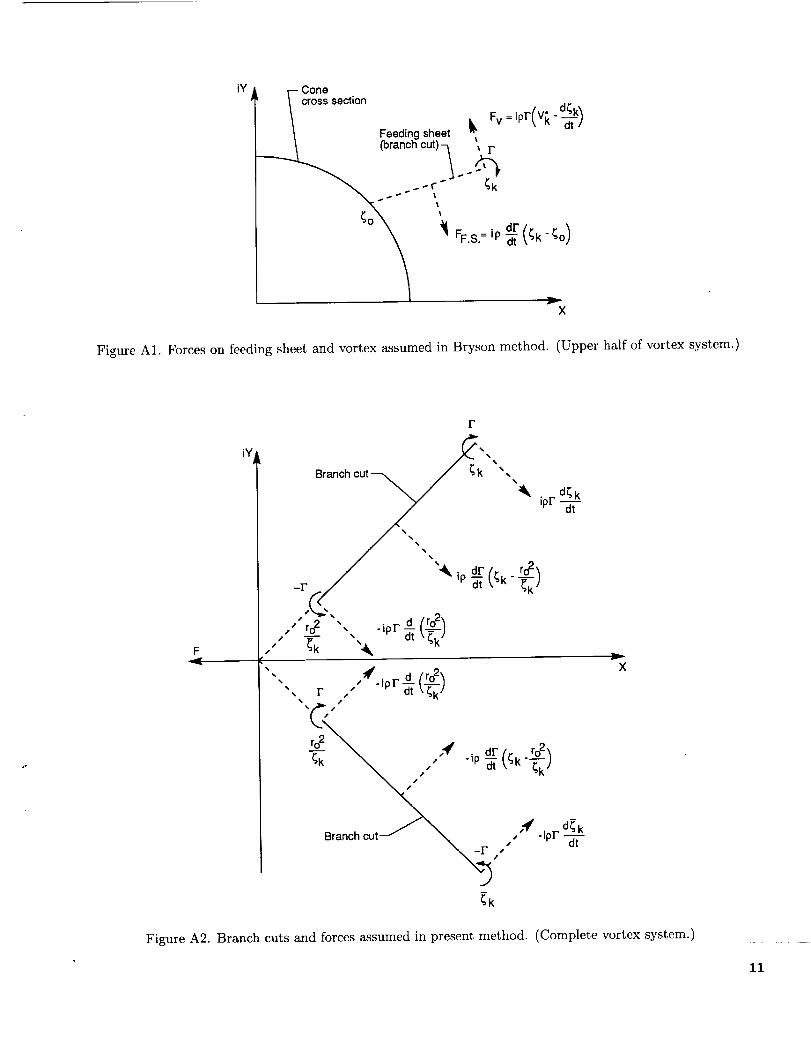
Zero-Force Condition Used by Bryson

The zero-force condition used to determine vor-

tex positions and strengths in a concentrated vortexmodel is based on the principle that an isolated po-tential vortex should sustain no force. (See ref. 7.) Inthe Bryson method (ref. 10), the zero-force equationis developed by installing a feeding sheet (fig. A1) andbalancing out the force on the feeding sheet with anequal and opposite force on the vortex. This feedingsheet is assumed to be the path along which vor-ticity is fed into the primary vortex and acts as amathematical branch cut, which is needed to makethe velocity potential for the system single-valued.There is a discontinuity in ¢ equal to the circulationstrength across this branch cut, and since F varieswith distance along the cone axis, ¢ also varies withthis distance. Since time and distance along the coneaxis are related (see eq. (9) of text), there will be, ac-cording to the unsteady Bernoulli equation, a pres-sure difference across the feeding sheet of

aT

dp = p-_ (A1)

When integrated over the length of the feeding sheet,this pressure difference results in a pressure force of

.aTFF.s.= - (A2)

Bryson required that this force be balanced out byan equal and opposite force at the vortex center.

The force at the vortex center arises from a non-

zero local-flow velocity at the center, and accordingto the Kutta-Joukowski theorem, is given by

Fv = ipF V_ - dt ](A3)

This force consists of two parts: (1) the force ipFV_is due to the induced effects at the vortex center.

(Here, Vk*, the induced velocity, is equal to the free-stream crossflow velocity plus the velocities inducedby all of the singularities in the system, except theprimary vortex itself; the velocity induced by a pri-mary vortex at its own center is assumed to be zero.)

The force -ipF_ is due to the absolute motion(2)of the vortex center.

Combining equations (A2) and (A3) gives thefollowing zero-force equation used by Bryson:

-'p-_ (Ck - G) + ipF V{ - dCk'_dt ] =0 (A4)

Zero-Force Condition Used in PresentMethod

The zero-force equation used by Bryson repre-sents one way of resolving the problem of how tomake the velocity potential single-valued and at thesame time ensure zero net force on the vortex system.This solution is not completely satisfactory, however,since it requires a pressure force on the feeding sheetthat is balanced out only "in the mean" to get zeronet force on the vortex system. In the present paper,a new approach is taken; the branch cut is assumedto lie between the primary vortex and its image (in-stead of between the primary vortex and a separa-tion point). Then, when the equation for the forceson the vortex system is written out, it shows thatthe pressure force on the branch cut is actually partof the change in momentum that the vortex system

undergoes in response to the force exerted on it bythe body. Therefore, the pressure force should notbe balanced out. (See fig. (A2).)

The momentum of a pair of vortices of equal cir-culation strength is equal to the product of the fluiddensity, the circulation, and the distance between thevortices. (See refs. 18 and 19.) For the system shownin figure (A2), the total momentum is given by thefollowing:

MV = ipF ( _k - r2 _k]- ipr (_k -- r2°_-_k](A5)

The force F that the body exerts on the fluid isequal to the rate of change of momentum. Taking thederivative of MV with respect to time and expandingthe results gives

- _pl _- + (A6)

If the branch cuts are taken between the primaryvortices and their images, as shown in figure (A2),the first term in equation (A6) can be interpretedas a force on the upper branch cut and the sec-ond term as a force on the lower branch cut. These

forces are of the same form as Bryson's feeding-sheet

9

force (eq. (A2)), but they act over the distance be-

tween the primary and image vortices instead of the

length _k --_o. The terms ipF_ and -ipF_t inequation (A6) can be interprete_ as forces caused

by the absolute motion of the primary vortices; like-

wise, the terms--iPF_t_\_k] and ipF_ (_)can

be interpreted as forces associated with the motion

of the image vortices. (These forces are shown as

dashed vectors in fig. (A2) because, in accordance

with d'Alembert's principle, they are effective forces,

equal but opposite in direction to rates of change in

momentum, rather than actual forces.)

The effective forces shown in figure (A2) combinewith the force F that the body exerts on the fluid to

form a system in equilibrium. Since these forces are

in equilibrium, there cannot be an additional force

that is due to induced effects acting at the vortex

center; if there were, the force on the body would not

be equal to that given by the momentum theorem.

The zero-force condition to impose with the vor-

tex system in figure (A2), therefore, is that there canbe no force due to induced effects acting at the vortex

center. For the cone in the present study, this con-

dition was imposed by requiring that each primary

vortex move as a free vortex, that is, at a velocityequal to the local flow velocity at its center:

V_ = d_k (AT)dt

In the present method, the feeding sheet has es-

sentially been removed from consideration; a feeding

sheet per se is not considered necessary with this typeof concentrated vortex model. The branch cut from

the primary vortex center to its image vortex center

serves to make the velocity potential single-valued.And while the vortices are assumed to be fed in some

way so that their circulation strengths increase with

distance along the cone axis, the actual manner in

which they are fed is not considered important. In

the actual flow, vorticity is fed into primary vortices

along curved feeding sheets, as best depicted in the

vortex , cloud or the free vortex sheet methods. In

those methods, however, as in the present method,there are no pressure forces associated with the feed-

ing sheets that would have to be balanced out bya force on the vortex. The curved sheets in thos_methods are assumed to be free surfaces that cannot

sustain a pressure force.

Also, the requirement that there be no force due

to induced effects at the vortex center does not

necessarily mean that the vortex moves with the local

crossflow velocity in all types of flow fields. In an

unsteady flow field, the vortex velocity must be equal

to the local flow velocity at a given instant; however,

since the vortex can also undergo motions caused byunsteady effects, the vortex velocity, in general, is not

equal to the local flow velocity. The requirement of

equation (AT), therefore, does not necessarily apply

to problems such as the vortex flow over cylindersand narrow delta wings, where other constraints on

the vortex system may have to be considered.

10

iY

,branchout)

_s ,_o-_(_ _ol

Figure A1. Forces on feeding sheet and vortex assumed in Bryson method. (Upper half of vortex system.)

F

iY

r

Branch cut _ k" __,,,,

""'... ,o_. i_,'_'_'_

-r t _'_k _k )

" , d (ro_/,/ ro2 , -ipF-_ \_k /.," _k "._

"" , "Np' - d (ro2_,, _ , -,p=-- _,=---)

_ i / clt r_k

¢,_.',,,rr°2 _ ,4 • drl,. ro2_

_k ,,,,, "'P-_ _,_k_)

/,4 -ior d_k

_k

X

Figure A2. Branch cuts and forces assumed in present method. (Complete vortex system.)

11

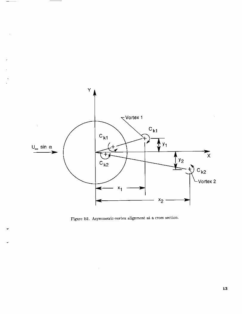
Appendix B

Extension of Zero-Force Condition to

Asymmetric Vortices

The zero-force condition on which the presentmethod is based--that the primary vortices moveas free vortices_an be extended to include vor-

tices that have different circulation strengths and areasymmetrically aligned about the y = 0 axis. (Seefig. B1.) This is done by writing a zero-force equa-tion similar to equations (14) and (15) at each of thetwo primary vortex centers as follows:

At vortex 1,

rl 1 / tandfUITallCkl+al2Ck2= _o rl/ro t--_ cos 01 (B1)

(rl 1 ) tan_sin01 (B2)V1 _- bll Ckl -I- bl2Ck2 = r-o rl/ro tan _

At vortex 2,

U2+a21C_l+a22C_= _o r27ro _cosO_

V2+b21Ckl +b22Ck2 = _ r27ro _-_sin02 (B4)

Combining equations (B1) and (B2) gives thefollowing equation:

(all tan01 - bll)Ckl + (a12 tan01

- bl2)Ck2 = - (U1 tan01 -- Yl) (B5)

Combining equations (B3) and (B4) gives thefollowing equation:

(a21 tan02 -- b21)ekl + (a22 tan02

- b22) Ck2 = - (U2 tan 02 - V2) (B6)

Equations (B5) and (B6) can be solved simultane-ously to give the circulation strengths C1 and C2 forassumed primary vortex positions. Equations (B1)and (B3) can then be solved to give the following val-ues of tan _/tan _ (designated by subscripts 1 and 2for vortices 1 and 2, respectively).

From equation (B1),

tan_ (rl/ro-- rl@o)c°sO1

t--_n_ ] l = U1 + a11Ck1 + al2Ck2(B7)

From equation (B3),

tan (_ (r2/ro--r_@ro)c°s02ta_n_]2 = U2 + a21Ckl + a22Ck2 (B8)

A solution is obtained when the vortex centers arelocated such that

tana_ = (tan_tantf] 1 \ t-a-_n_ ] 2

(B9)

Asymmetric solutions have been obtained usingthe basic Bryson equations in reference 20. Solutions

using the general asymmetric form of the presentmethod have been obtained in reference 21.

=

=

12

Y

Uoosin a

Ckl

Ck2

•Vortex 1

x 1

Ckl

Yl

x 2

XY2

Ck2

2

Figure B1. Asymmetric-vortex alignment at a cross section.

13

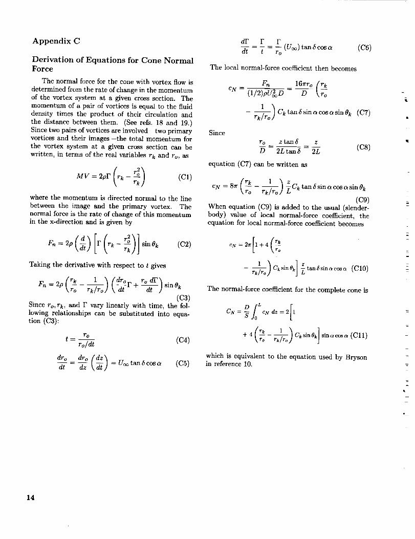
Appendix C

Derivation of Equations for Cone NormalForce

The normal force for the cone with vortex flow is

determined from the rate of change in the momentumof the vortex system at a given cross section. The

momentum of a pair of vortices is equal to the fluiddensity times the product of their circulation and

the distance between them. (See refs. 18 and 19.)Since two pairs of vortices are involved--two primaryvortices and their images--the total momentum forthe vortex system at a given cross section can be

written, in terms of the real variables rk and ro, as

( rd_ (C1)MV = 2pF r k- rk ]

where the momentum is directed normal to the line

between the image and the primary vortex. Thenormal force is the rate of change of this momentumin the x-direction and is given by

Fn=2p(d) [F(rk r2_lsinOk (C2)

Taking the derivative with respect to t gives

(r k 1 ) (droF ro dF_Fn = 2p _o rk/ro \dt + dt ] sin 0k

(c3)Since ro, rk, and F vary linearly with time, the fol-

lowing relationships can be substituted into equa-tion (C3):

ro

t- ro/dt (C4)

..o..o-_- = d---z = U_ tan 6 cos _ (C5)

dF F F

dt t ro(Uoc) tan 6 cos a (C6)

The local normal-force coefficient then becomes

Fn 167fro (r kCN = (1/2)P U2 D -- -D _o

1)rk/r ° Ck tan 6 sin a cos a sin 0k (C7)

Since

ro z tan

D 2L tan

equation (C7) can be written as

2L (C8)

r k 1 ) zcN = 87r _o rk/ro -LCktan_sinac°sv_sinOk

(c9)When equation (C9) is added to the usual (slender-body) value of local normal-force coefficient, theequation for local normal-force coefficient becomes

1) ].r_ro GsinOk Z tan 6sin a cosa (C10)

The normal-force coefficient for the complete cone is

°/? [CN = -_ C N dz = 2 1

+4(r-_o ra--/ro1 ) CksinOk]sin'c°s"(CII)

which is equivalent to the equation used by Brysonin reference 10.

!

v

=

IL

i

14

References

1. McRae, David S.: The Conically Symmetric Navier Stokes

Numerical Solution for Hypersonic Cone Flow at High

Angle of Attack. AFFDL-TR-76-139, U.S. Air Force,

Mar. 1977. (Available from DTIC as AD A042 072.)

2. McRae, D. S.; Peake, D. J.; and Fisher, D. F.: A

Computational and Experimental Study of High Reynolds

Number Viscous/Inviscid Interaction About a Cone at

High Angle of Attack. AIAA-80-1422, July 1980.

3. Peake, David J.; Owen, F. Kevin; and Higuchi,

Hiroshi: Symmetrical and Asymmetrical Separations

About a Yawed Cone. High Angle of Attack Aerodynam-

ics, AGARD-CP-247, Jan. 1979, pp. 16-1-16-27.

4. Fiddes, S. P.: A Theory of the Separated Flow Past a Slen-

der Elliptic Cone at Incidence. Computation of Viscous-

lnviscid Interactions, AGARD-CP-291, Feb. 1981,

pp. 30-1-30-14.

5. Smith, J. H. B.: Theoretical Modelling of Three-

Dimensional Vortex Flows in Aerodynamics. Aerodynam-

ics of Vortical Type Flows in Three Dimensions, AGARD-

CP-342, July 1983, pp. 17-1-17-21.

6. Dyer, D. E.; Fiddes, S. P.; and Smith, J. H. B.: Asymmet-

ric Vortex Formation b'_rom Cones at Incidence--A Simple

lnviscid Model. Tech. Rep. 81130, British Royal Aircraft

Establ., Oct. 1981.

7. Smith, J. H. B.: Improved Calculations of Leading-

Edge Separation From Slender Delta Wings. Tech. Rep.

No. 66070, British Royal Aircraft Establ., Mar. 1966.

8. Mendenhall, Michael R.; and Lesieutre, Daniel J.: Predic-

tion of Vortex Shedding From Circular and Noncircular

Bodies in Subsonic Flow. NASA CR-4037, 1987.

9. Mendenhall, Michael R.; and Perkins, Stanley C., Jr.:

Vortex Cloud Model for Body Vortex Shedding and Track-

ing. Tactical Missile Aerodynamics, Michael J. Hemsch

and Jack N. Nielsen, eds., American Inst. of Aeronautics

and Astronautics, Inc., c.1986, pp. 519-571.

10. Bryson, A. E.: Symmetric Vortex Separation on Circular

Cylinders and Cones. Trans. ASME, Ser. E: J. Appl.

Mech., vol. 26, no. 4, Dec. 1959, pp. 643-648.

11. Moore, Katharine: Line- Vortex Models of Separated

Flow Past a Circular Cone at Incidence. Tech. Memo.

Aero 1917, British Royal Aircraft Establ., Oct. 1981.

12. Rainbird, W. J.; Crabbe, R. S.; and Jurewicz, L. S.:

A Water Tunnel Investigation of the Flow Separation

About Circular Cones at Incidence. N.R.C. No. 7633

(Aeronaut. Rep. LR-385), National Research Council of

Canada, Sept. 1963.

13. Milne-Thomson, L. M.: Theoretical Hydrodynamics, Fifth

ed. Revised. Macmillan Press Ltd., 1968.

14. Wu, Jain-Ming; and Lock, Robert C.: A Theory for

Subsonic and Transonic Flow Over a Cone--With and

Without Small Yaw Angle. RD-74-2 (Proj. No. (DA)

1M262303A214), Tennessee Univ. Space Inst., Dec. 1973.

(Available from DTIC as AD 776 374.)

15. Sarpkaya, qMrgut: Separated Flow About Lifting Bodies

and Impulsive Flow About Cylinders. AIAA J., vol. 4,

no. 3, Mar. 1966, pp. 414-420.

16. Batchelor, G. K.: An Introduction to Fluid Dynamics.

Cambridge Univ. Press, 1970.

17. FSppl, Ludwig: Vortex Motion Behind a Circular Cylin-

der. NASA TM-77015, 1983.

18. Von Khrmgn, Th.; and Sears, W. R.: Airfoil Theory for

Non-Uniform Motion. J. Aeronuat. Sci., vol. 5, no. 10,

Aug. 1938, pp. 379-390.

19. Sarpkaya, T.: An Analytical Study of Separated Flow

About Circular Cylinders. Trans. ASME, Ser. D: J. Basic

Eng., vol. 90, no. 4, Dec. 1968, pp. 511-520.

20. Dyer, D. E.; Fiddes, S. P.; and Smith, J. H. B.: Asymmet-

ric Vortex Formation From Cones at Incidence_A Sim-

ple Inviscid Model. Aeronaut. Q., vol. XXXIII, pt. 4,

Nov. 1982, pp. 293-312.

21. Chin, S.; and Lan, C. Edward: Calculation of Symmetric

and Asymmetric Vortex Separation on Cones and Tangent

Ogives Based on Discrete Vortex Models. NASA CR-4122,

1988.

15

XF -F

Y

(X

(a) System of axes.

r

Z

Yrk

U_ sin (_

F

X

.._ -r

(b) Vortex-system geometry in crossflow plane.

Figure 1. Schematic of vortex-flow model.

16

Yk/ro

Uoosin _ F Cone surface

.6

.4

.2

Constant C kConstant tan a/tan

FSppl curve

I I 1 I I I.2 .4 .6 .8 1.0 1.2 1.4 1.6

xk/r o

I I1.8 2.0

Figure 2. Solution field of vortex-center locations for different values of C k and tan c_/tan 5.

17

.8 ._ Constant C k"_ .... Constant tan a/tan5

, _ ........ F6ppl curve

.6 .0 O

\1 ;\4._-,,'s'° ..

Yk/r° "4 F _2"0_2.5_ ,_5._"'"I , ,&_,. 4.4.'°.6

nl.4J/ t_,# ,"2 n / Is_"• I I I,' ,"2

I / #t, °° "

.__ | i1#,"

1 2 ,,_,_

o 1 I I1.0 1.2 1.4 1.6

xk/r o

(a) 5 = 7.5 °.

.8 I_ Constant C k| _. Constant tana/tan

/ ^',_ ........ F_l oo_,.

°F\',,

1.4 ,-'*'"

21--1 o 0 '"• /n t _,,,,:2

/' ,' ,t""I #, °1.2--_ .',.."

I ;,'='"

o _"/" I I Iv

1.O 1.2 1.4 1.6

xk/r o

(b) 5=12.5 ° .

Figure 3. Comparison of calculated and measured vortex-center locations.

18

Cs

150

140

130

120

110

100

5, deg

(_ 7.5

9o I I I I I0 1 2 3 4 5

tan a/tan

(a) Cs versus tan a/tan _.

.6

.5

.4

C k .3

.2

.1

_, deg

7.512.5

I I I I I0 1 2 3 4 5

tan a/tan 5

(b) Ck versus tan a/tan _.

Figure 4. Variation of separation-point location and nondimensional vortex strengths with tan a� tan _.

19

Ck

1.5

1.0

,5

0

1.0

Yk/ro .5

0

0

s"

Jt I I I I

(E_SDO-O0O 0I I I I 1

Experiment (ref. 11)Present method

Bryson method (ref. 20)

fI I, I I 1

(_2_>-o-o-£r o1 I I I

=

xk/r o

1.5

1.0

.5

(_t30--0-0-0 0

I I I I I I I I I ,I0 1 2 3 4 5 0 1 2 3 4 5

tan cz/tan 5 tan 0_/tan 5

(a) _ = 7.5°. (b) 5=12.5 ° .

Figure 5. Nondimensional vortex strengths and vortex-center locations determined from experimental separa-

tion points given in figure 4(a).

20

U si n ,,,_.._

Point vortices(vortex cloud)

(a) Oz-----10°.

|

!

(b) o_= 20°.

Figure 6. Comparison of vortex rollup depicted by vortex cloud method (refs. 7 and 8) with streamlinescalculated using present method. 5 = 5°.

21

U sin

z

(c) a = 30°.

Figure 6. Concluded.

=

22

= 30 °

Present method

Vortex cloud(ref. 8)

©

c N .3a. = 20 °

= 10 °

I I I I.4 .6 .8 1.0

z/L

(a) 5 = 5°.

Figure 7. Comparison of local normal-force coefficients calculated using present method and vortex cloud

method.

23

Present method

a = 30 °

.5 Vortex cloud(ref. 8) _

.4

= 22.5 °

CN .3

.2

.1

0

I 1 I 1.2 .4 16 .8

z/L

(b) 5 = 7.So.

Figure 7. Concluded.

I1.0

24

C k

1.0

.8

.6

.4

.2

oC

0 Present methodr-I vortex cloud (ref. 8)

r

I I I 1 I

tan o_/tan 8

(a) Ck versus tan a� tan 6.

I I7 8

C N

2.0

1.5

1.0

.5

$

ched flow

I I I I I I I1 2 3 4 5 6 7 8

tan o_/tan 8

(b) CN versus tan a� tan 6.

Figure 8. Comparison of total normal-force coefficients calculated using present method and vortex cloudmethod. 6 = 5 °.

25

C k

1.0

.2

O Present methodI--I Vortex cloud (ref. 8)

Bryson method (ref. 10)

.8

.6

.4

o' I I5 6

tan a/tan 8

(a) Ck versus tan a/tan 5.

I7

18

2.0

1.5

C N 1.0

.5

F

I I01_ 1 2 3 4 5 6 7 - 8

tan (z/tan 8

Attached flow

(b) CN versus tan a/tan 5.

Figure 9. Comparison of total normal-force coefficients calculated using present method and vortex cloudmethod. 5 = 7.5 °.

26

Report DocumentationPageF4afionar Aeronaul_cs and

Space Adrn_n,s_ration

1. ReportNAsANO.TP_2989 2. Government Accession No. 3. Recipient's Catalog No.

4. Title and Subtitle

Discrete-Vortex Model for the Symmetric-Vortex Flow on Cones

7. Author(s)

Thomas G. Gainer

9. Performing Organization Name and Address

NASA Langley Research CenterHampton, VA 23665-5225 11.

12. Sponsoring Agency Name and Address 13.

National Aeronautics and Space AdministrationWashington, DC 20546-0001 14.

5. Report Date

May 1990

6. Performing Organization Code

8. Performing Organization Report No.

L-16586

10. Work Unit No.

505-60-21-06

Contract or Grant No.

Type of Report and Period Covered

Technical Paper

Sponsoring Agency Code

15. Supplementary Notes

16. Abstract

A relatively simple but accurate potential-flow model has been developed for studying thesymmetric-vortex flow on cones. The model is a modified version of the model first developed byBryson, in which discrete vortices and straight-line feeding sheets were used to represent the flowfield. It differs, however, in the zero-force condition used to position the vortices and determinetheir circulation strengths. The Bryson model imposed the condition that the net force on thefeeding sheets and discrete vortices must be zero. The proposed model satisfies this zero-forcecondition by having the vortices move as free vortices, at a velocity equal to the local crossflowvelocity at their centers. When the free-vortex assumption is made, a solution is obtained in theform of two nonlinear algebraic equations that relate the vortex-center coordinates and vortexstrengths to the cone angle and angle of attack. The vortex-center locations calculated usingthe model are in good agreement with experimental values. The cone normal forces and centerlocations are in good agreement with the vortex cloud method of calculating symmetric flow fields.

17. Key Words (Suggested by Authors(s))

Aeronautics

Aerodynamics

18. Distribution Statement

Unclassified--Unlimited

Subject Category 02

19. Security Classif. (of this report)Unclassified 120 SecurityClassif"(°f this page)Unclassified 121 N°' °f Pages122"Price27 A03

NASA FORM 1626 OCT

For sale by the National Technical Information Service, Springfield, Virginia 22161-2171

NASA-Langley,1990

2

!:-