Eur. Phys. J. D 23, 421–436 (2003)DOI: 10.1140/epjd/e2003-00065-1 THE EUROPEAN

PHYSICAL JOURNAL D

Discrete gap solitons in a diffraction-managed waveguide array

P.G. Kevrekidis1, B.A. Malomed2,a, and Z. Musslimani3

1 Department of Mathematics and Statistics, University of Massachusetts, Amherst MA 01003-4515, USA2 Department of Interdisciplinary Studies, Faculty of Engineering, Tel Aviv University, Tel Aviv 69978, Israel3 Department of Applied Mathematics, University of Colorado, Campus Box 526, Boulder CO 80309-0526, USA

Received 14 September 2002 / Received in final form 4 February 2003Published online 24 April 2003 – c© EDP Sciences, Societa Italiana di Fisica, Springer-Verlag 2003

Abstract. A model including two nonlinear chains with linear and nonlinear couplings between them, andopposite signs of the discrete diffraction inside the chains, is introduced. In the case of the cubic [χ(3)]nonlinearity, the model finds two different interpretations in terms of optical waveguide arrays, based on thediffraction-management concept. A continuum limit of the model is tantamount to a dual-core nonlinearoptical fiber with opposite signs of dispersions in the two cores. Simultaneously, the system is equivalent toa formal discretization of the standard model of nonlinear optical fibers equipped with the Bragg grating.A straightforward discrete second-harmonic-generation [χ(2)] model, with opposite signs of the diffractionat the fundamental and second harmonics, is introduced too. Starting from the anti-continuum (AC) limit,soliton solutions in the χ(3) model are found, both above the phonon band and inside the gap. Solitonsabove the gap may be stable as long as they exist, but in the transition to the continuum limit theyinevitably disappear. On the contrary, solitons inside the gap persist all the way up to the continuumlimit. In the zero-mismatch case, they lose their stability long before reaching the continuum limit, butfinite mismatch can have a stabilizing effect on them. A special procedure is developed to find discretecounterparts of the Bragg-grating gap solitons. It is concluded that they exist at all the values of thecoupling constant, but are stable only in the AC and continuum limits. Solitons are also found in theχ(2) model. They start as stable solutions, but then lose their stability. Direct numerical simulations inthe cases of instability reveal a variety of scenarios, including spontaneous transformation of the solitonsinto breather-like states, destruction of one of the components (in favor of the other), and symmetry-breaking effects. Quasi-periodic, as well as more complex, time dependences of the soliton amplitudes arealso observed as a result of the instability development.

PACS. 05.45.Yv Solitons – 42.50.Md Optical transient phenomena: quantum beats, photon echo,free-induction decay, dephasings and revivals, optical nutation, and self-induced transparency –63.20.Ry Anharmonic lattice modes

1 Introduction

1.1 Objectives of the work

Solitary-wave excitations in discrete nonlinear dynami-cal models (lattices) is a subject of great current inter-est, which was strongly bolstered by experimental ob-servation of solitons in arrays of linearly coupled opticalwaveguides [1] and development of the diffraction man-agement (DM) technique, which makes it possible to effec-tively control the discrete diffraction in the array, includ-ing a possibility to reverse its sign (make the diffractionanomalous) [2,3]. It has recently been shown that a latticesubject to periodically modulated DM can also supportstable solitons, both single-component ones [4,5] and two-component solitons with nonlinear coupling between thecomponents via the cross-phase-modulation (XPM) [6].

a e-mail: malomed@eng.tau.ac.il

Two-component nonlinear-wave systems, both contin-uum and discrete, which feature a linear coupling betweenthe components, constitute a class of media which can sup-port gap solitons (GSs). A commonly known example ofa continuum medium that gives rise to GSs is a nonlinearoptical fiber carrying a Bragg grating [7,8], whose stan-dard model is based on the equations

iΨt + iΨx +(|Ψ |2 + 2|Φ|2)Ψ + Φ = 0,

iΦt − iΦx +(|Φ|2 + 2|Ψ |2)Φ+ Ψ = 0, (1)

where Ψ(x, t) and Φ(x, t) are amplitudes of the right- andleft-propagating waves, and the Bragg-reflection coeffi-cient is normalized to be 1. Another optical system thatmay give rise to GSs is a dual-core optical fiber with asym-metric cores, in which the dispersion coefficients have op-posite signs [9].

422 The European Physical Journal D

In this work, we demonstrate that the use of the DMtechnique provides for an opportunity to build a dou-ble lattice in which two discrete subsystems with oppo-site signs of the effective diffraction are linearly coupled,thus opening a way to theoretical and experimental studyof discrete GSs, as well as of solitons of different types(solitons in linearly coupled lattices with identical discretediffraction in the two subsystems have recently been con-sidered in Ref. [10]; a possibility of the existence of discreteGSs in a model of a nonlinear-waveguide array consistingof alternating cores with two different values of the prop-agation constant was also considered recently [11]). Theobjective of the work is to introduce this class of systemsand find fundamental solitons in them, including the in-vestigation of their stability. We will also consider, in amore concise form, another physically relevant possibility,viz., a discrete system with a second-harmonic-generating(SHG) nonlinearity, in which the diffraction has oppositesigns at the fundamental and second harmonics. Solitonswill be found and investigated in the latter system too.

It is relevant to start with equations on which our χ(3)

model (the one with the cubic nonlinearity) is based,

idψn

dt= − (C∆2 + q)ψn

−(|ψn|2 + β |φn|2

)ψn − κφn = 0, (2)

idφn

dt= δ (C∆2 + q)φn

−(|φn|2 + β |ψn|2

)φn − κψn = 0, (3)

where ψn(t) and φn(t) are complex dynamical variablesin the two arrays (sublattices), κ and β being coeffi-cients of the linear and XPM coupling between them,and t is actually not time, but the propagation distancealong waveguides, in the case of the most physically rele-vant optical interpretation of the model. The operatorsC∆2ψn ≡ C (ψn+1 + ψn−1 − 2ψn) and (−δ)C∆2φn ≡(−δ)C (φn+1 + φn−1 − 2φn) represent discrete diffractioninduced by the linear coupling between waveguides insideeach array, the diffraction being normal in the first sublat-tice and anomalous in the second, with a negative relativediffraction coefficient −δ and intersite coupling constant C(one may always set C > 0, which we assume below).Physical reasons for having −δ < 0 are explained below.Finally, the real coefficient q accounts for a wavenumbermismatch between the sublattices.

We also choose a similar SHG model, following thewell-known pattern of discrete SHG systems with normaldiffraction at both harmonics [12,13]:

idψn

dt= −C∆2ψn − ψ�

nφn, (4)

2idφn

dt= δC∆2φn − ψ2

n − κφn, (5)

where the asterisk stands for the complex conjugationand κ is a real mismatch parameter. In this case too, weassume −δ < 0.

Fig. 1. Two parallel asymmetric arrays of optical waveguidesthat are described by equations (2, 3), provided that parallelbeams propagate obliquely across both arrays. Arrows indicatemisaligned directions at which light is coupled into the arrays;inside them, both propagation directions are identical.

There are at least two different physical realizations ofthe χ(3) model based on equations (2, 3). First, one mayconsider two parallel arrays of nonlinear waveguides withdifferent effective values n(1) and n(2) of the refractive in-dex in them corresponding to a given (oblique) directionof the light propagation. To this end, the waveguides be-longing to the two arrays may be fabricated from differ-ent materials; alternatively, they may simply differ by thetransverse size of waveguiding cores, or by the refractiveindex of the filling between the cores, see, e.g., Figure 1.The difference in the effective refractive index gives riseto the mismatch parameter q in equations (2, 3). Moreimportantly, it may also give rise to different coefficientsof the discrete diffraction. Indeed, the DM technique as-sumes launching light into the array obliquely, the effectivediffraction coefficient in each array being [2]

D(1,2) = 2Cd2 cos(k

(1,2)⊥ d

), (6)

where d is the spacing of both arrays, and k(1,2)⊥ are trans-

verse components of the two optical wave vectors. As itfollows from equation (6), the diffraction coefficients aredifferent if k(1)

⊥ �= k(2)⊥ .

Despite the fact that k(1)⊥ and k

(2)⊥ are assumed dif-

ferent, we assume that the propagation directions of thelight beams are parallel in the two arrays, as a conspicu-ous walkoff (misalignment) between them will easily de-stroy any coherent pattern. On the other hand, the lightcoupled into both arrays has the same frequency, hencethe absolute values of the two wave vectors are related asfollows: k(1)/k(2) = n(1)/n(2), where n(1,2) are the above-mentioned effective refractive indices. Combining the lat-ter relation and the classical refraction law, and takinginto regard the condition that the propagation directionsare parallel inside the arrays, one readily arrives at theconclusion that

k(1)⊥ /k

(2)⊥ = n(1)/n(2). (7)

Note that the two incidence angles θ(1,2) (at the interfacebetween the arrays and air) are related in a similar way,

P.G. Kevrekidis et al.: Discrete gap solitons in a diffraction-managed waveguide array 423

(sin θ(1))/(sin θ(2)) = n(1)/n(2), hence the incident beams(in air) must be misaligned, in order to be aligned in thearrays.

Equation (6) shows that there is a critical direction ofthe beam in each array, corresponding to k

(1,2)⊥ d = π/2,

at which the effective diffraction coefficient changes itssign [2]. Due to the difference between k

(1)⊥ and k

(2)⊥ , the

critical directions are different in the two arrays. Then, ifthe common propagation direction in the arrays is chosento be between the two critical directions, equation (6) givesdifferent signs of the two diffractive coefficients. Note thatthis interpretation of the model implies no XPM couplingbetween the arrays, i.e., β = 0 in equations (2, 3).

An alternative realization is possible in a single array ofbimodal optical fibers, into which two parallel beams withorthogonal polarizations, u and v, are launched obliquely.If the two polarizations are circular ones, then β = 2 inequations (2, 3), and the asymmetry between the beams,which makes it possible to have different signs of the co-efficient (6) for them, may be induced by birefringence,which, in turn, can be easily generated by twist appliedto the fibers [14]. The birefringence also gives rise to themismatch q. As for the linear mixing between the two po-larizations, which is assumed in the model, it can be easilyinduced if the fibers are, additionally, slightly deformed,having an elliptic cross-section [14]. If the two polariza-tions are linear, then the birefringence is induced by theelliptic deformation, and the linear mixing is induced bythe twist, the XPM coefficient being 2/3 in this case (as-suming that, as usual, the birefringence makes it possibleto neglect four-wave mixing nonlinear terms [14]).

It is interesting to note that the discrete model basedon equations (2, 3) with κ = 0 is exactly tantamountto a formal discretization of the above-mentioned con-tinuum model which was introduced in reference [9] todescribe a dual-core optical fiber with opposite signs ofdispersion in the cores. Another quite noteworthy featureof the present model is that, if β = 2, it turns out tobe formally equivalent to a discretization of the standardBragg-grating model (1), which is produced by replac-ing Ψx → (Ψn+1 − Ψn−1) /2 and Φx → (Φn+1 − Φn−1) /2.Indeed, making the substitution (“staggering transforma-tion”)

Ψn ≡ inφn, Φn ≡ inψn, (8)

one concludes that the discrete version of equations (1)takes precisely the form of equations (2, 3) with δ = 1,q = 2C, κ = 1, and β = 2.

1.2 The linear spectrum

Before proceeding to the presentation of numerical resultsfor solitons found in the system of equations (2, 3), it isrelevant to understand at which values of the propagationconstant Λ (spatial frequency) solitons with exponentiallydecaying tails may exist in this model. There are two re-gions in which they may be found. Firstly, inside the gapof the system’s linear spectrum one may find discrete gap

solitons, i.e., counterparts of the GSs found in the con-tinuum version of the model in reference [9]. Secondly,solitons specific to the discrete model may be found abovethe phonon band. To analyze these possibilities, an asymp-totic expression for the tail,

ψn, φn ∼ exp (iΛt− λ |n|) (9)

is to be substituted into the linearized version of equa-tions (2, 3).

Investigating the possibility of the existence of solitonsabove the phonon gap, it is sufficient to focus on the par-ticular case δ = 1 and q = 0, when the system’s spectrumtakes a simple form (we have also considered more generalcases with positive δ different from 1 and q �= 0, concludingthat they do not yield anything essentially different fromthis case). The final result, produced by a straightforwardalgebra, is that solitons are possible in the region

Λ2 > Λ2edge ≡ 16C2 + κ2, (10)

±Λedge being edges of the phonon band. In what followsbelow, we will assume Λ > 0, as in this case positive andnegative values of Λ are equivalent.

To understand the possibility of the existence of thediscrete GSs, we, first, set δ = 1 as above, but keep themismatch q as an arbitrary parameter. Then, the gap iseasily found to be

Λ2 < Λ2gap ≡

q2 + κ2 if q < 0,

κ2 if 0 ≤ q ≤ 4C,

(q − 4C)2 + κ2 if q > 4C

(11)

(recall that, by definition, C > 0). An essential role of themismatch parameter is that it makes the gap broader if itis negative.

In the more general case, δ �= 1, two different layerscan be identified in the gap, similar to what was found inthe continuum limit [9]. For instance, if q = 0, the innerand outer layers are

0 < Λ2 <4δ

(δ + 1)2κ2, and

4δ(δ + 1)2

κ2 < Λ2 < κ2 (12)

(in the case δ = 1, the outer layer disappears). The differ-ence between the layers is the same as in the continuumlimit [9]: in the outer layer, solitons, if any, have mono-tonically decaying tails, i.e., real λ in equation (9), whilein the inner layer λ is complex, and, accordingly, solitontails are expected to decay with oscillations.

1.3 The structure of the work

The rest of the paper is organized as follows. In Section 2,we display results for solitons found above the phononband, i.e., in the region (10). The evolution of the soli-tons is monitored, starting from the anti-continuum (AC)limit C = 0, and gradually increasing C. Any branch

424 The European Physical Journal D

of soliton solutions in this region must disappear, ap-proaching the continuum limit. Indeed, as the radiationband (frequently called “phonon band”, referring to linearphonon modes in the lattice dynamics) becomes infinitelybroad in this limit, see equation (10), the solution branchwith Λ = const will crash hitting the swelling phononband. However, in many cases the soliton of this type isfound to remain stable as long as it exists, so it may beeasily observed experimentally in the optical array.

In Section 3 we present results for solitons existing in-side the gap. In the outer layer [which is defined as perEq. (12), provided that δ �= 1], we were able to find onlysolitons of an “antidark” type, that sat on top of a non-vanishing background. However, in the inner layer [recallit occupies the entire gap in the case δ = 1, according toEq. (12)], true solitons are easily found (in accord with theprediction, their tails decay with oscillations). In the caseq = 0, these solutions appear as stable ones in the AClimit, get destabilized at some finite critical value of C,and continue, as unstable solutions, all the way up to thecontinuum limit, never disappearing. It is quite interestingthat sufficiently large negative mismatch strongly extendsthe stability range for these solitons.

As was mentioned above, the χ(3) model based onequations (2, 3) may be considered as a discretization ofthe standard gap-soliton system (1). In this connection, itis natural to search for discrete counterparts of the usualGSs in the latter system. However, the discrete GSs foundin Section 3 do not have any counterpart in the continuumsystem (1), as the staggering transformation (8) makes di-rect transition from the discrete equations (2, 3) to thecontinuum system (1) impossible. At the end of Section 3,we specially consider discrete solitons which are directlyrelated to GSs in the system (1). We find that such soli-tons exist indeed at all the values of C, their drastic differ-ence from those found in Sections 2 and 3 is that they areessentially complex solutions to the stationary version ofequations (2, 3). At all finite values of C, they are unsta-ble, but the instability asymptotically vanishes in the ACand continuum limits, C → 0 and C → ∞.

In Section 4, we briefly consider the SHG model (4, 5).Solitons are found in this model too, and their stabilityis investigated. When the solitons are linearly unstable,the development of their instability is examined (in allSects. 2, 3, and 4) by means of direct numerical sim-ulations, which show that the instability may initiate atransition to a localized breather, or to lattice turbulence,or, sometimes, complete decay of the soliton into latticephonon waves.

2 Solitons above the phonon band

2.1 General considerations

Stationary solutions to equations (2, 3) are sought for theform

ψn = eiΛtun, φn = eiΛtvn, (13)

where Λ is the propagation constant defined above. Infigures displayed below, the stationary solutions will becharacterized by the norms of their two components,

P 2u ≡

+∞∑n=−∞

u2n, P 2

v ≡+∞∑

n=−∞v2

n . (14)

Once such solutions are numerically identified by meansof a Newton-type numerical scheme, we then proceed toinvestigate their stability, assuming that the solution isperturbed as follows:

ψn = [un + εan exp(iωt)+εbn exp(−iω�t)] exp(iΛt), (15)

φn = [vn + εcn exp(iωt) + εdn exp(−iω�t)] exp(iΛt),(16)

where ε is an infinitesimal amplitude of the perturba-tion, and ω is the eigenvalue corresponding to the lin-ear (in)stability mode. The set of the resulting linearizedequations for the perturbations {a, b�, c, d�;ω} is subse-quently solved as an eigenvalue problem. This is done byusing standard numerical linear algebra subroutines builtinto mathematical software packages [15]. If all the eigen-values ω are purely real, the solution is marginally stable;on the contrary, the presence of a nonzero imaginary partof ω indicates that the soliton is unstable. When the so-lutions were unstable, their dynamical evolution was fol-lowed by means of fourth-order Runge-Kutta numericalintegrators, to identify the development and outcome ofthe corresponding instabilities.

In what follows below, we describe different classes ofsoliton solutions, which are generated, in the AC limit, byexpressions with different symmetries. Still another classof solitons, which carries over into the usual GSs in thecontinuum system (1), will be considered in the next sec-tion.

2.2 Solution families which are symmetricin the anti-continuum limit

As it was said above, in this section we set δ = 1 andq = 0, since comparison with more general numericallyfound results has demonstrated that this case adequatelyrepresents the general situation, as concerns the existenceand stability of solitons. Figure 2 shows a family of solitonsolutions found for κ = 0.1, Λ = 2 and β = 0, as a functionof the coupling constant C. In this case, the family starts,in the AC limit (C = 0), with a solution that consists of asymmetric excitation localized at a single lattice site n0,with

un0 = vn0 = ±√Λ− κ

1 + β, (17)

and terminates at finite C. Figure 2 demonstrates thatthis branch is always unstable. The termination of thebranch happens when it comes close to the phonon band,that swells with the increase of C. The branch terminates

P.G. Kevrekidis et al.: Discrete gap solitons in a diffraction-managed waveguide array 425

0 0.05 0.1 0.15 0.2 0.25 0.3 0.35 0.4 0.450.5

1

1.5

2

P

C

40 45 50 55 60

0

0.5

1

1.5

u n , v n

n −4 −2 0 2 4−1

−0.5

0

0.5

1

ωi

ωr

40 45 50 55 60

0

0.5

1

1.5

u n , v n

n−4 −2 0 2 4

−0.4

−0.2

0

0.2

0.4

ωi

ωr

0 0.05 0.1 0.15 0.2 0.25 0.3 0.35 0.4 0.450

0.1

0.2

0.3

0.4

0.5

0.6

0.7

0.8

0.9

1

ωi

C

Fig. 2. The top panel shows the norms Pu (lower curve) and Pv

(upper curve) of the two components of the soliton solutionvs. C, up to the point where the branch terminates. The nextset of panels shows two examples of the solution at C = 0.1(the upper row) and C = 0.464 (just near the terminationpoint of the branch; the lower row), together with the spectralplanes of the corresponding linear stability eigenvalues (thevertical and horizontal coordinates in the plane correspond tothe imaginary and real parts of ω). The profiles of the un and vn

components are shown, respectively, by circles and stars. Thesesolutions are always unstable. The bottom panel shows theimaginary part of the single unstable eigenfrequency vs. C.

at C = 0.464, when the upper edge of the band is atΛedge =

√κ2 + 16C2 ≈ 1.859, according to equation (10).

This value is still smaller than the fixed value of the soli-ton’s propagation constant, Λ = 2, for which the solitonbranch is displayed in Figure 2. The branch, if it could becontinued, would crash into the upper edge of the phononband at C = 0.499. The slightly premature terminationof this soliton family is a consequence of the nonlinearcharacter of the solutions, as the above prediction for thetermination point was based on the linear approximation.

Fig. 3. Evolution of the unstable soliton from Figure 2 in thecase C = 0.1, β = 0, and κ = 0.1. The top panel showsthe fields’ spatial profiles (the circles correspond to |ψn|2, andthe stars to |φn|2) for t = 4 (left panel), t = 192 (middle panel)and t = 196 (right panel). The first profile is nearly identical tothe initial condition, while the other two were chosen close topoints where the oscillating amplitude of the resultant breatherattains its maximum and minimum. The bottom panel showsthe field evolution at the central lattice site (n = 50), clearlydemonstrating the breathing nature of the established state.The solid and dashed lines are, respectively, |ψ50|2 and |φ50|2.In this case, the instability growth rate of the initial soliton is≈0.8; in view of this large value, it was not necessary to addany initial perturbation to trigger the instability.

An example of the development of the instability ofthis solution, as found from direct simulations of the fullequations (2, 3), is given in Figure 3 for C = 0.1. It isclearly seen that the unstable soliton turns into a stablebreather.

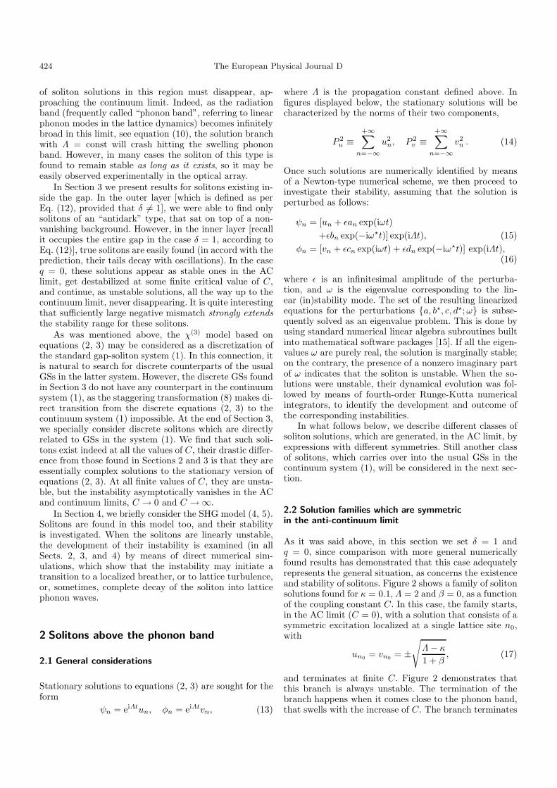
On the contrary, in the presence of XPM with thephysically relevant value of β = 2, a similar solutionbranch, found for the same values κ = 0.1 and Λ = 2,is stable for all C, until it terminates at C = 0.499. Notethat, at this point, the upper edge (10) of the phonon bandis Λedge = 1.999, which is extremely close to Λ = 2, i.e.,the termination of the solution family is indeed accountedfor by its crash into the swelling phonon band. Details ofthis stable branch are shown in Figure 4.

Direct simulations of this solution have corroboratedits stability (details are not shown here). In fact, in allthe cases when solitons are found to be stable in termsof the linearization eigenvalues (see other cases below),direct simulations fully confirm their dynamical stability.

2.3 Solution families which are anti-symmetricin the anti-continuum limit

Another branch of solutions is initiated, in the AC limit,by an anti-symmetric excitation localized at a single

426 The European Physical Journal D

0 0.1 0.2 0.3 0.4 0.50

0.5

1

1.5

P

C

40 45 50 55 60

0

0.5

1

u n , v n

n−3 −2 −1 0 1 2 3

−2

0

2

ωi

ωr

30 40 50 60 70

−0.2

0

0.2

u n , v n

n−4 −2 0 2 4

−4

−2

0

2

4

ωi

ωr

Fig. 4. The same as in Figure 2, but for the case β = 2. Themiddle and lower panels display examples of the soliton solu-tions at C = 0.1 and C = 0.499, respectively. In the top panel,the upper and lower curves now correspond to the vn and un

components, i.e., opposite to the case shown in Figure 1. Noticethat this branch is always stable until it terminates, thereforethe figure does not contain a counterpart of the dependenceshown in the bottom panel of Figure 2.

lattice site, cf. equation (17):

un0 = −vn0 = ±√Λ+ κ

1 + β· (18)

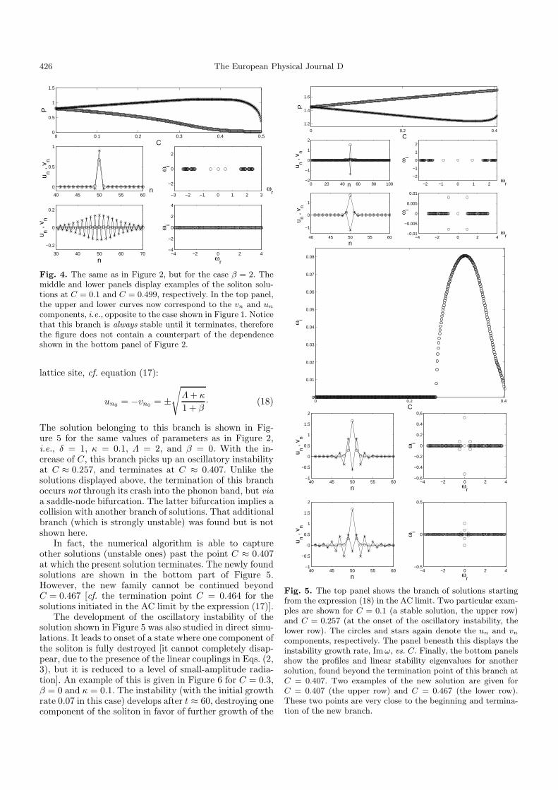
The solution belonging to this branch is shown in Fig-ure 5 for the same values of parameters as in Figure 2,i.e., δ = 1, κ = 0.1, Λ = 2, and β = 0. With the in-crease of C, this branch picks up an oscillatory instabilityat C ≈ 0.257, and terminates at C ≈ 0.407. Unlike thesolutions displayed above, the termination of this branchoccurs not through its crash into the phonon band, but viaa saddle-node bifurcation. The latter bifurcation implies acollision with another branch of solutions. That additionalbranch (which is strongly unstable) was found but is notshown here.

In fact, the numerical algorithm is able to captureother solutions (unstable ones) past the point C ≈ 0.407at which the present solution terminates. The newly foundsolutions are shown in the bottom part of Figure 5.However, the new family cannot be continued beyondC = 0.467 [cf. the termination point C = 0.464 for thesolutions initiated in the AC limit by the expression (17)].

The development of the oscillatory instability of thesolution shown in Figure 5 was also studied in direct simu-lations. It leads to onset of a state where one component ofthe soliton is fully destroyed [it cannot completely disap-pear, due to the presence of the linear couplings in Eqs. (2,3), but it is reduced to a level of small-amplitude radia-tion]. An example of this is given in Figure 6 for C = 0.3,β = 0 and κ = 0.1. The instability (with the initial growthrate 0.07 in this case) develops after t ≈ 60, destroying onecomponent of the soliton in favor of further growth of the

0 0.2 0.4

1.2

1.4

1.6

P

C

0 20 40 60 80 100−2

−1

0

1

2

u n , v n

n −2 −1 0 1 2

−2

−1

0

1

2

ωi

ωr

40 45 50 55 60

−1

0

1

u n , v n

n−4 −2 0 2 4

−0.01

−0.005

0

0.005

0.01

ωi

ωr

0 0.2 0.40

0.01

0.02

0.03

0.04

0.05

0.06

0.07

0.08

ωi

C

40 45 50 55 60−1

−0.5

0

0.5

1

1.5

2

u n , v n

n−4 −2 0 2 4

−0.6

−0.4

−0.2

0

0.2

0.4

0.6ω

i

ωr

40 45 50 55 60−1

−0.5

0

0.5

1

1.5

2

u n , v n

n−4 −2 0 2 4

−0.5

0

0.5

ωi

ωr

Fig. 5. The top panel shows the branch of solutions startingfrom the expression (18) in the AC limit. Two particular exam-ples are shown for C = 0.1 (a stable solution, the upper row)and C = 0.257 (at the onset of the oscillatory instability, thelower row). The circles and stars again denote the un and vn

components, respectively. The panel beneath this displays theinstability growth rate, Imω, vs. C. Finally, the bottom panelsshow the profiles and linear stability eigenvalues for anothersolution, found beyond the termination point of this branch atC = 0.407. Two examples of the new solution are given forC = 0.407 (the upper row) and C = 0.467 (the lower row).These two points are very close to the beginning and termina-tion of the new branch.

P.G. Kevrekidis et al.: Discrete gap solitons in a diffraction-managed waveguide array 427

0 20 40 60 80 100 120 140 160 180 2000

0.5

1

1.5

2

2.5

3

|ψ50

|2 , |φ

50|2

t

45 50 550

0.5

1

1.5

2

2.5

3

|ψn|2 ,

|φn|2

n30 40 50 60 70

0

0.5

1

1.5

2

2.5

3

|ψn|2 ,

|φn|2

n

Fig. 6. Dynamical development of the oscillatory instabilityof the anti-symmetric solution for C = 0.3, β = 0 and κ = 0.1.The meaning of the symbols is as in Figure 3. The top leftand right panels show the field configuration at t = 4 andt = 196, respectively. The bottom panel once again shows thefield evolution at the central site.

other one. In this case, a uniformly distributed noise per-turbation of an amplitude 10−4 was added to acceleratethe onset of the instability, as the initial instability is veryweak (which implies that the unstable soliton may be ob-served in experiment).

A counterpart of the solution from Figure 5, but withβ = 2, rather than β = 0, is shown in Figure 7. Thisbranch is always unstable (i.e., in the case of the solu-tions starting from the anti-symmetric expression in theAC limit, the XPM nonlinearity destabilizes the solitons,while in the case of the branch that was initiated by thesymmetric expression in the AC limit, the same XPMnonlinearity was stabilizing). It terminates at C ≈ 0.219,again through a saddle-node bifurcation. As in the previ-ous case, a new family of solutions can be captured by thenumerical algorithm past the termination point. The newfamily is found for 0.22 < C < 0.498, and it is also shownin Figure 7. Comparing the value Λedge = 1.995 given byequation (10) in this case with the actual value Λ = 2 ofthe soliton’s propagation constant, we conclude that thetermination of the latter branch is caused by its collisionwith the phonon band. Notice also that the latter branchbecomes unstable only very close to its termination point,at C > 0.494.

In the case of β = 2, direct simulations show thatthe instability of the anti-symmetric branch gives rise torearrangement of the solution into a very regular breathershown in Figure 8 for C = 0.1 and κ = 0.1.

2.4 Solution families which are asymmetricin the anti-continuum limit

Additional branches of the solutions may start in the AClimit from asymmetric configurations, provided that Λ isstill larger, namely for Λ > 2κ. In particular, such anextra branch can be initiated by the following AC-limit

0 0.1 0.2

0.4

0.6

0.8

1

1.2

P

C

40 45 50 55 60−1

0

1

u n , v n

n −2 0 2−0.5

0

0.5

ωi

ωr

45 50 55

−1

−0.5

0

n−2 0 2

−0.5

0

0.5

ωi

ωr

u n , v n

0 0.1 0.20

0.05

0.1

0.15

0.2

0.25

0.3

0.35

0.4

0.45

0.5

ωi

C

40 45 50 55 60

0

0.5

1

1.5

u n , v n

n−2 0 2

−3

−2

−1

0

1

2

3

ωi

ωr

40 45 50 55 60

0

0.5

1

1.5

u n , v n

n−5 0 5

0ωi

ωr

Fig. 7. The same as in Figure 5, but for β = 2. This branch isalways unstable (as is shown by the middle plot demonstratingthe instability growth rate vs. C) in its range of existence,0 < C < 0.219. Examples of the solution displayed in theupper part of the figure are given for C = 0.1 and C = 0.219.The lower part shows the new solution family found past thetermination point of the unstable branch. Example of the newsolutions are given for C = 0.22 (stable, the upper row) andC = 0.498 (just prior to the termination of the new family, thelower row). The instability of this branch sets in at C ≈ 0.494,i.e., very close to the termination point.

428 The European Physical Journal D

0 20 40 60 80 100 120 140 160 180 2000

0.2

0.4

0.6

0.8

1

1.2

1.4

t

|ψ50

|2 , |φ

50|2

45 50 550

0.5

1

1.5

|ψn|2 ,

|φn|2

n45 50 55

0

0.5

1

1.5

n45 50 55

0

0.5

1

1.5

n

Fig. 8. The development of the instability accounted for bythe imaginary eigenfrequency (with the growth rate ≈ 0.45) ofthe anti-symmetric branch, in the case of C = 0.1, κ = 0.1.The top panels pertain to t = 4 (left), t = 100 (middle) andt = 120 (right). The latter two have again been chosen closeto the points where the oscillating amplitude of the resultantbreather attains its maximum and minimum, respectively. Theinstability sets in around t ≈ 40; no external perturbation wasadded to the initial condition in this case.

solution excited at a single site n = n0 (here, β = 0), cf.equations (17, 18):

u2n0

=12

[Λ ±

√Λ2 − 4κ2

], (19)

vn0 = κ−1(Λun0 − u3n0

) . (20)

An example of this solution for the upper sign in equa-tion (19) is shown, for Λ = 2, κ = 0.5 and δ = 1, inFigure 9. Such asymmetric branches may be stable forsufficiently weak coupling (in this case, for C < 0.204),but they eventually become unstable, and disappear soonthereafter (at C ≈ 0.213, in this case).

The evolution of the instability (for C > 0.204) for thisasymmetric branch is strongly reminiscent of that shownin Figure 3, resulting in a persistent breathing state.

The branch that commences from the AC expres-sion (19) with the lower sign is shown for Λ = 2, κ = 0.75and δ = 1 in Figure 10. The branch remains stable as longas it exists, i.e., for C < 0.46. At this point, it disappearscolliding with the phonon band, whose upper edge is lo-cated, according to equation (10), at Λedge ≈ 1.987, whichis very close to the family’s fixed propagation constant,Λ = 2.

3 Gap solitons

3.1 Solitons in the inner layer of the gap

All the solutions that were examined in the previous sec-tion had their propagation constant above the upper edgeof the phonon spectrum. Another issue of obvious interest

0 0.05 0.1 0.15 0.2

0.5

1

1.5

P

C

40 45 50 55 60

0

0.5

1

1.5

u n , v n

n−4 −2 0 2 4

−1

−0.5

0

0.5

1

ωi

ωr

40 45 50 55 60

0

0.5

1

1.5

u n , v n

n−4 −2 0 2 4

−1

−0.5

0

0.5

1

ωi

ωr

0 0.1 0.20

0.1

0.2

0.3

0.4

0.5

0.6

ωi

C

Fig. 9. The solution branch generated, in the AC limit, bythe asymmetric expressions (19, 20) with the upper sign. Thenotation is the same as in Figure 2. Two examples of the solu-tion are shown for C = 0.1 and C = 0.213. The most unstableeigenvalue is shown, vs. C, in the bottom panel. The instabilitysets in at C ≈ 0.204, and the branch terminates at C ≈ 0.213.

is to study possible gap solitons (GSs), whose propagationconstant is located inside the gap (11), i.e., below the loweredge of the phonon band. Unlike the solitons found abovethe band, GSs may persist up to the continuum limit.

An example of such a solution for Λ = 0.75, κ = −1,δ = 0.9, and β = 0 is shown in Figure 11. In the AC limit,this branch starts with the expression (17). The branchis stable for small C, but then it becomes unstable dueto oscillatory instabilities. The first two instabilities occurat C = 0.242 and C = 0.349, as is shown in Figure 11.Past the onset of the instabilities, this branch continuesto exist (as an unstable one) indefinitely with the increaseof C, and carries over into an (unstable) GS in the con-tinuum limit. At large values of C, the distinct phononbands, which are clearly seen in the example of the eigen-value spectrum shown for C = 0.4 in Figure 11, eventuallycollide, and their opposite Krein signs (see the definitionand discussion of these in Ref. [16]), give rise to a whole

P.G. Kevrekidis et al.: Discrete gap solitons in a diffraction-managed waveguide array 429

0 0.05 0.1 0.15 0.2 0.25 0.3 0.35 0.4 0.450

0.5

1

1.5

C

P

40 45 50 55 60

0

0.5

1

u n , v n

n−4 −2 0 2 4

−1

0

1

ωi

ωr

30 40 50 60 70

−0.2

0

0.2

u n , v n

n−4 −2 0 2 4

−1

0

1

ωr

ωi

Fig. 10. The same as in Figure 9, but generated by the ex-pression (19) with the lower sign. This solution is always stableuntil it terminates at C ≈ 0.458. Examples of the solution forC = 0.2 and C = 0.458 (the latter case is chosen just prior tothe termination of the branch) are shown, as usual, by meansof their profiles and linear stability eigenfrequencies.

set of oscillatory instabilities. The result is clearly seen inthe example of the eigenvalue spectrum shown in the bot-tom panel of Figure 11 for a large value of the couplingconstant, C = 4. The characteristic size of the instabilitygrowth rate (largest imaginary part of the eigenvalue) isnearly the same for C = 0.4 and C = 4, in the latter caseit being ≈ 0.09. Notice, however, that, as the continuumlimit is approached, the instabilities may be suppressed, ina part or completely, by finite-size effects (for an exampleof such finite-size restabilization, see Ref. [17]).

The development of the oscillatory instability of GSbelonging to the inner layer is displayed, for C > 0.242,in Figure 12 for C = 0.4, δ = 0.9, κ = −1 and β = 0. Inthis particular case, there are two oscillatory instabilitieswhose growth rates are in the interval 0.1 < ωi < 0.2. Asa result, symmetry breaking occurs, resulting in a shift ofthe central position of the soliton (from the site n = 50to n = 49). Oscillatory features in the dynamics are alsoobserved in the latter case, and a small amount of energyis emitted as radiation.

Similar results were obtained for smaller values of Λ,for instance, Λ = 0.25. It was verified too that this sce-nario persists in the presence of the XPM nonlinearity(i.e., for β = 2), as it is shown in Figure 13. In the lattercase, the evolution of the instability with the increase of Cis quite interesting, as it is nonmonotonic. The instabilityfirst arises at C ≈ 0.11 (due to a collision between discreteeigenvalues with opposite Krein signs). Subsequent resta-bilization takes place at C ≈ 0.16, but the solutions areunstable again for C > 0.36, and remain unstable there-after, up to the continuum limit.

In the case of β = 2, the dynamical development of theoscillatory instabilities is similar to the β = 0 case, againdemonstrating symmetry-breaking effects.

0 0.05 0.1 0.15 0.2 0.25 0.3 0.35 0.4 0.45 0.5

1.4

1.6

1.8

P

C

40 45 50 55 60−0.5

0

0.5

1

1.5

u n , v n

n −4 −2 0 2 4−1

−0.5

0

0.5

1

ωi

ωr

40 45 50 55 60−0.5

0

0.5

1

1.5

u n , v n

n−4 −2 0 2 4

−0.5

0

0.5

ωi

ωr

0 0.05 0.1 0.15 0.2 0.25 0.3 0.35 0.4 0.45 0.50

0.1

0.2

ωi

C

30 35 40 45 50 55 60 65 70−0.5

0

0.5

1

1.5

2

2.5

u n , v n

n

−15 −10 −5 0 5 10 15−0.1

0

0.1

ωi

ωr

Fig. 11. The branch of the gap-soliton solutions with Λ = 0.75,κ = −1, δ = 0.9, and β = 0. The upper part of the figureshows the norms of the two components of the soliton, andexamples of the solutions for C = 0.1 (stable) and C = 0.4(after the onset of the first oscillatory instability). The middlepanel shows the instability growth rates, while the lower partof the figure gives an example of a solution belonging to thisbranch, found at a much larger value of the coupling constant,C = 4. This solution family extends, as an unstable one, up tothe continuum limit.

430 The European Physical Journal D

0 20 40 60 80 100 120 140 160 180 2000

0.5

1

1.5

2

2.5

3

t

|ψ50

|2 , |φ

50|2

45 50 550

0.5

1

1.5

2

2.5

|ψn|2 ,

|φn|2

n40 50 60

0

0.5

1

1.5

2

2.5

n30 40 50 60 70

0

0.5

1

1.5

2

2.5

n

Fig. 12. The evolution of the unstable gap soliton belong-ing to the inner layer, for C = 0.4, δ = 0.9, κ = −1, andβ = 0. The top panels shows the wave field distribution att = 4 (left), t = 124 (middle) and t = 132 (right). Symmetry-breaking effects are clearly visible. A random perturbation ofan amplitude 10−4 was added to the initial condition in orderto catalyze the onset of the instability, which occurs at t > 40.

3.2 Solutions in the outer layer of the gap

In all the cases considered in the previous subsections,the soliton’s propagation constant Λ belonged to the innerlayer of the gap, see equation (12). We have also examinedthe situation when Λ belongs to the outer layer defined inequation (12) (the outer layer exists unless δ = 1). Anexample is shown in Figure 14, where β = 0, κ = −1,δ = 0.1, and Λ ≈ 0.787 is chosen to be in the middleof the outer layer. In this case, we typically obtained de-localized solitons, sitting on top of a finite background(they are sometimes called “antidark” solitons). As canbe observed from Figure 14, such solutions may be stablefor sufficiently weak coupling, but become unstable as thecontinuum limit is approached, although they do not dis-appear in this limit (in Ref. [9] such delocalized solitonswere found in the continuum counterpart of the presentmodel).

The instability development in the case of the outer-layer GSs is demonstrated, for C = 0.549, β = 0, κ = −1and δ = 0.1, in Figure 15. In this case, the non-vanishingbackground is also perturbed by the instability, resultingin, plausibly, chaotic oscillations throughout the lattice.Symmetry-breaking effects, which shift the central peakfrom its original position, are observed too in this case.

3.3 Stabilization of the gap solitons by mismatch

The above considerations show that, inside the inner layerof the gap, it is easy to identify families of soliton solu-tions that persist in the continuum limit as C → ∞. How-ever, all the examples considered above showed that thesolutions get destabilized at finite C and remain unstable

0 0.2 0.4 0.6 0.8 1 1.2 1.4 1.6 1.8 20.5

1

1.5

2

P

C

40 45 50 55 60−0.5

0

0.5

1

u n−v n

n −3 −2 −1 0 1 2 3−0.5

0

0.5

ωi

ωr

40 45 50 55 60−0.5

0

0.5

1

1.5

u n−v n

n−10 −5 0 5 10

−0.5

0

0.5

ωi

ωr

0 0.05 0.1 0.15 0.2 0.25 0.3 0.35 0.4 0.45 0.50

0.02

0.04

0.06

0.08

0.1

0.12

0.14

0.16

0.18

Max

i(ωi)

C

Fig. 13. The same as the previous figure, but for β = 2. Exam-ples of the solutions are shown for C = 0.2 (upper row, stable)and C = 1.6 (lower row, unstable due to several oscillatory in-stabilities). The bottom panel demonstrates the nonmonotonicevolution of the instability of this solution with the increaseof C.

40 45 50 55 60−0.5

0

0.5

1

1.5

u n , v n

n−4 −2 0 2 4

−1

−0.5

0

0.5

1

ωi

ωr

40 45 50 55 60−0.5

0

0.5

1

1.5

2

u n , v n

n−4 −2 0 2 4

−0.2

−0.1

0

0.1

0.2

ωi

ωr

Fig. 14. Solutions with non-decaying oscillatory backgroundfor propagation constants belonging to the outer layer definedby equation (12). The top panel shows a stable solution forC = 0.158, and the bottom panel shows an unstable one ofC = 0.576. These solutions are unstable for all C > 0.341.

P.G. Kevrekidis et al.: Discrete gap solitons in a diffraction-managed waveguide array 431

0 20 40 60 80 100 120 140 160 180 2000

0.5

1

1.5

2

2.5

3

3.5

|ψ50

|2 , |φ

50|2

t

30 40 50 60 700

0.5

1

1.5

2

2.5

3

|ψn|2 ,

|φn|2

n0 20 40 60 80 100

0

0.2

0.4

0.6

0.8

1

|ψn|2 ,

|φn|2

n

Fig. 15. The time evolution of the outer-layer gap solitons forC = 0.549, β = 0, κ = −1 and δ = 0.1. The initial condition isperturbed by a random uniformly distributed perturbation ofan amplitude 10−4. The result of the instability is the excita-tion of background oscillations, as well as a shift of the soliton’speak from its original position. The top left and right spatialprofiles correspond to t = 4 and t = 200, respectively.

with the subsequent increase of C. Therefore, a challeng-ing problem is to find solution families that would remainstable for large values of C.

In fact, the introduction of a finite mismatch q (recallit was set equal to zero in all the examples consideredabove) may easily stabilize the discrete GSs. To this end,we pick up a typical example, with C = 0.5, κ = −1,δ = 0.5, Λ = 0.75, and β = 0, when the GS exists but isdefinitely unstable in the absence of the mismatch. Fig-ures 16 and 18 show the effect of positive and negativevalues of the mismatch on the solitons. As is seen, largevalues of the positive mismatch can make the instabilityvery weak, but cannot completely eliminate it. However,sufficiently large negative mismatch readily makes the soli-tons truly stable. Thus, adding the negative mismatch isthe simplest way to stabilize the solitons at large C, whichis not surprising, as equation (11) demonstrates that thenegative mismatch makes the gap broader.

As an example of the dynamical evolution of unstablesolitons in the case of positive mismatch, in Figure 17 wedisplay the case of C = 0.5, κ = −1, β = 0, δ = 0.5 andq = 1. In this case, the evolution leads to the establishmentof a breather with a rather complex dynamical behavior.

The instability development in the case of negativemismatch, q = −2.5, is demonstrated in Figure 19. A lo-calized breather with quasi-periodic intrinsic dynamics isobserved in this case as an eventual state.

3.4 Discrete counterparts of gap solitonsfrom the Bragg-grating model

As was shown in the introduction, the particular case ofequations (2, 3) with κ = 1, δ = 1, and β = 2 may beinterpreted, with regard to the transformation (8), as a

0 0.5 1 1.5 2 2.5 3 3.5 4 4.5 50.5

1

1.5

2

P

q

0 0.5 1 1.5 2 2.5 3 3.5 4 4.5 50

0.1

0.2

0.3

Max

i(ωi)

q

40 45 50 55 60−0.5

0

0.5

1

1.5

2

u n , v n

n−4 −2 0 2 4

−0.5

0

0.5

ωi

ωr

40 45 50 55 60−1

0

1

2

u n , v n

n −4 −2 0 2 4−0.02

−0.01

0

0.01

0.02

ωi

40 45 50 55 60−0.5

0

0.5

1

1.5

2

u n , v n

n−5 0 5

−4

−2

0

2

4x 10

−3

ωi

ωr

ωr

Fig. 16. A family of the gap-soliton solutions obtained forfixed values C = 0.5, κ = −1, δ = 0.5, Λ = 0.75, and β = 0, bycontinuation to positive values of the mismatch parameter q.The top panel and the one beneath it show the evolution of thenorms of the two components of the solution, and of the largestinstability growth rate, with the increase of q. Other panelsshow examples of the solution (as usual, in terms of profiles ofthe two components and linear stability eigenvalues) for q = 0,q = 2, and q = 5, from top to bottom.

discretization of the standard Bragg-grating system (1).This continuum model gives rise to a family of exact GSsolutions [7],

Ψ = U(x) exp (−it cos θ) ,Φ = V (x) exp (−it cos θ) , (21)

U(x) =sin θ√

3sech

(x sin θ − i

2θ

),

V = −U∗, (22)

where the real parameter θ takes values 0 < θ < π. Apart of this interval, 0 < θ < θcr ≈ 1.01 (π/2), is filledwith stable solitons [18], while the remaining part containsunstable ones.

All the discrete GSs considered above are not coun-terparts of the continuum solitons given by equa-tions (21, 22). Establishing a direct correspondence

432 The European Physical Journal D

0 20 40 60 80 100 120 140 160 180 2000

1

2

3

4

5

6

t

|ψ50

|2 , |φ

50|2

30 40 50 60 700

1

2

3

4

5

|ψn|2 ,

|φn|2

n30 40 50 60 70

0

1

2

3

4

5

|ψn|2 ,

|φn|2

n

Fig. 17. The dynamical evolution in the unstable case withC = 0.5, κ = −1, β = 0, δ = 0.5 and q = 1 (positive mismatch).The top left and right panels correspond to t = 4 and t = 396,respectively. A complex pattern of the amplitude evolution isobserved in this case. The initial condition contains a randomperturbation with an amplitude 5 × 10−5.

−5 −4.5 −4 −3.5 −3 −2.5 −2 −1.5 −1 −0.5 00.5

1

1.5

2

2.5

3

P

q

−5 −4.5 −4 −3.5 −3 −2.5 −2 −1.5 −1 −0.5 00

0.05

0.1

0.15

0.2

0.25

Max

i(ωi)

q

40 45 50 55 60−0.5

0

0.5

1

1.5

2

u n , v n

n−4 −2 0 2 4

−0.4

−0.2

0

0.2

0.4

ωi

ωr

40 45 50 55 60

0

0.5

1

1.5

2

2.5

u n , v n

n−5 0 5

−0.1

−0.05

0

0.05

0.1

ωi

ωr

40 45 50 55 60

0

1

2

3

u n , v n

n−10 −5 0 5 10

−1

−0.5

0

0.5

1

ωi

ωr

Fig. 18. The same as in Figure 16, but for negative values ofthe mismatch. Examples of the solutions are given for q = 0,q = −2, and q = −5, from top to bottom.

0 50 100 150 200 250 300 350 4000

0.5

1

1.5

2

2.5

t

|ψ50

|2 , |φ

50|2

30 40 50 60 700

0.5

1

1.5

2

2.5

|ψn|2 ,

|φn|2

n30 40 50 60 70

0

0.5

1

1.5

2

2.5

|ψn|2 ,

|φn|2

n

Fig. 19. The evolution of the unstable discrete gap solitonin with C = 0.5, κ = −1, β = 0, δ = 0.5 and q = −2.5(negative mismatch). The top left and right panels show thefield profiles for t = 4 and t = 196, respectively. The timeevolution of the amplitudes is shown in the bottom panel. Arandom perturbation of an amplitude 10−4 was used in thiscase.

between the latter ones and discrete solitons of equa-tions (2, 3) is complicated by two problems: the trans-formation (8) does not have a continuum limit, and realsymmetric or anti-symmetric GSs with |Λ| < κ do not ex-ist in the AC limit, as is seen from equations (17, 18), i.e.,the usual starting point of the analysis is not available inthis case.

We have considered discrete analogs of the Bragg-grating GSs in the following way. First, we took a formaldiscrete counterpart of the waveforms (21) and (22), andused them as an initial guess, to generate numerically ex-act solutions of a direct discrete version of equations (1).Then the transformation (8) was applied to these solu-tions, and the result was used as an initial guess to find anumerically exact stationary solution of equations (2, 3)[as the discrete version of Eqs. (1), subject to the trans-formation (8), is tantamount to Eqs. (2, 3), the last stepwas engaged only to check the consistency of the numeri-cal scheme; the two solution are indeed completely identi-cal, see an example in Fig. 20]. This procedure naturallygenerates new discrete gap solitons, a crucial difference ofwhich from all the types considered above is that they aretruly complex solutions, see examples in Figures 20 and 21[to produce these examples, we started with θ = π/4 inEq. (22)].

Then, the solution was numerically continued, decreas-ing C, back to the AC limit, in order to identify its AC“stem”. The result is shown in Figure 21. Obviously, thisAC state is very different from all those considered above(in particular, it is complex).

Finally, linear-stability eigenvalues were calculated forthis new branch of the discrete GSs. The result (seeFig. 22) is that this branch is unstable for all finite valuesof C, getting asymptotically stable in both limits C → 0

P.G. Kevrekidis et al.: Discrete gap solitons in a diffraction-managed waveguide array 433

80 85 90 95 100 105 110 115 1200

0.05

0.1

0.15

0.2

0.25

|ψn|2

n

80 85 90 95 100 105 110 115 1200

0.05

0.1

0.15

0.2

0.25

|φn|2

Fig. 20. Absolute values of the fields in a new complex discretegap-soliton solution, which was obtained, at C = 1.24, from thediscretization of the Bragg-grating model (1) [the initial guessused a formal discrete counterpart of the expressions (22) withθ = π/4]. Then, the transformation (8) was applied to thissolution, and (in order to check the consistency of the numer-ical scheme) it was used as an initial condition of the Newtonmethod to find a solution to equations (2, 3). The continuousand dashed lines (which completely overlap) show the resultingprofiles generated by the procedure: one corresponds to the so-lution for the discrete version of the Bragg-grating model, andone to the direct solution of equations (2, 3).

and C → ∞ [large values of C are not shown in Fig. 22];the stability regained in the latter limit complies with theabove-mentioned fact that a subfamily of the continuumBragg-grating gap solitons are dynamically stable. Noticethat the natural norm of the continuum soliton differsfrom that of the discrete one, given by equation (14), by anadditional multiplier C−1/2 (which is proportional to theeffective lattice spacing). We have checked that the thusrenormalized norm of the soliton converges as C → ∞,although data for large C is not displayed in Figure 22.

4 Solitons in the model with the quadraticnonlinearity

Stationary solutions of the SHG system (4) and (5) arelooked for in an obvious form, cf. equations (13):

ψn = eiΛtun, φn = e2iΛtvn, (23)

and in this case we only consider the (most characteristic)case δ = 1. The linearization of equations (4, 5) demon-strates that one may expect termination of a soliton-solution branch, due to its collision with the phonon band,at (or close to) the point

Λ = κ/4 + C, (24)

and the gap between two phonon bands is

0 < Λ < κ/4 (25)

(it exists only if κ > 0).

80 90 100 110 120−0.5

0

0.5

Re,

Im(ψ

n)

80 90 100 110 120−0.5

0

0.5

Re,

Im(φ

n)

95 100 105−0.4

−0.2

0

0.2

0.4

Re,

Im(ψ

n)

95 100 105−0.4

−0.2

0

0.2

0.4

Re,

Im(φ

n)

n

−4 −2 0 2 4−0.2

−0.1

0

0.1

0.2

ωi

ωr

−2 −1 0 1 2−0.2

−0.1

0

0.1

0.2

ωi

ωr

Fig. 21. Left panels show profiles of real and imaginary partsof the fields ψn and φn in the discrete counterpart of the Bragg-grating gap soliton from Figure 20. Right panels show stabilityeigenvalues for the same soliton. The upper and lower parts ofthe figure pertain to the soliton at C = 1.24 (the same valueas in Fig. 20), and to its continuation to the anti-continuumlimit, C = 0. In the left panels, circles (joined by solid lines)refer to the real parts, and stars (connected by dashed lines)correspond to the imaginary parts of the corresponding fields.

0 0.2 0.4 0.6 0.8 1 1.2

0.5

0.6

0.7

0.8

0.9

1

1.1

1.2

P

C

0 0.2 0.4 0.6 0.8 1 1.20

0.05

0.1

0.15

0.2

0.25

0.3

0.35

Max

(ωi)

Fig. 22. The norm of the solution to equations (2, 3) which isthe discrete counterpart of the Bragg-grating gap soliton (up-per panel), and its two unstable eigenvalues (solid and dashedlines in the lower panel), vs. the coupling constant. Continua-tion of the figure to larger values of C shows that the solitonbecomes asymptotically stable as C → ∞.

Stationary solutions were constructed, again, by meansof continuation starting from the AC limit, where the ex-citation localized on a single site of the lattice assumes theform

vn0 = Λ, (26)

un0 = ±√vn0(4Λ− κ). (27)

Note that solutions with the propagation constant belong-ing to the gap (25) do not exist close to the AC limit.Indeed, the AC expression (27) shows that a necessary

434 The European Physical Journal D

0 0.005 0.01 0.015 0.020

0.2

0.4

0.6

P

C

40 45 50 55 60−0.1

0

0.1

0.2

u n , v n

n −0.4 −0.2 0 0.2 0.4−0.4

−0.2

0

0.2

0.4

ωi

ωr

40 45 50 55 60

−0.2

0

0.2

u n , v n

n−0.2 0 0.2

−0.05

0

0.05

ωi

ωr

0 0.005 0.01 0.015 0.020

0.01

0.02

0.03

0.04

0.05

ωi

C

Fig. 23. The family of the discrete SHG solitons found forκ = 0.9, δ = 1, and Λ = 0.25. The top panel shows the evo-lution of the norms of the fundamental- (circles) and second-frequency (stars) components of the soliton, which are definedthe same way as in equation (14), with the increase of C. Ex-amples of solutions are displayed for C = 0.01, below the in-stability threshold, which is Ccr = 0.015 (the upper row), andfor C = 0.024, just prior to the termination of the branch atC = 0.025 (the lower row). The bottom panel shows the evolu-tion of the instability growth rate (imaginary part of the mostunstable eigenvalue).

condition for its existence is 4Λ > κ. On the other hand,Λ stays in the gap (25) if 4Λ < κ, so the two conditionsare incompatible.

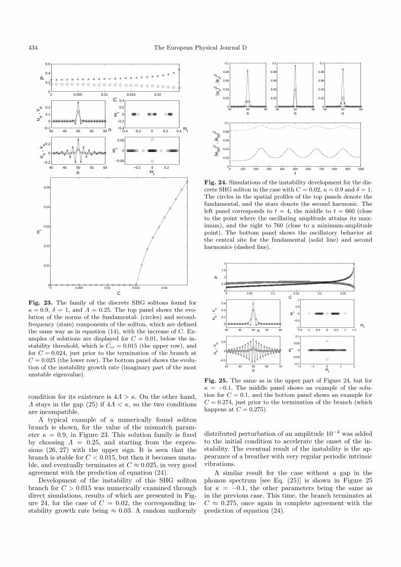
A typical example of a numerically found solitonbranch is shown, for the value of the mismatch param-eter κ = 0.9, in Figure 23. This solution family is fixedby choosing Λ = 0.25, and starting from the expres-sions (26, 27) with the upper sign. It is seen that thebranch is stable for C < 0.015, but then it becomes unsta-ble, and eventually terminates at C ≈ 0.025, in very goodagreement with the prediction of equation (24).

Development of the instability of this SHG solitonbranch for C > 0.015 was numerically examined throughdirect simulations, results of which are presented in Fig-ure 24, for the case of C = 0.02, the corresponding in-stability growth rate being ≈ 0.03. A random uniformly

0 100 200 300 400 500 600 700 800 900 10000

0.02

0.04

0.06

0.08

0.1

t

|ψ50

|2 , |φ

50|2

40 50 600

0.02

0.04

0.06

0.08

0.1

|ψn|2 ,

|φn|2

n40 50 60

0

0.02

0.04

0.06

0.08

0.1

n40 50 60

0

0.02

0.04

0.06

0.08

0.1

n

Fig. 24. Simulations of the instability development for the dis-crete SHG soliton in the case with C = 0.02, κ = 0.9 and δ = 1.The circles in the spatial profiles of the top panels denote thefundamental, and the stars denote the second harmonic. Theleft panel corresponds to t = 4, the middle to t = 660 (closeto the point where the oscillating amplitude attains its max-imum), and the right to 760 (close to a minimum-amplitudepoint). The bottom panel shows the oscillatory behavior atthe central site for the fundamental (solid line) and secondharmonics (dashed line).

0 0.05 0.1 0.15 0.2 0.250

0.5

1

1.5

2

P

C

40 45 50 55 60

0

0.2

0.4

0.6

u n , v n

n −1.5 −1 −0.5 0 0.5 1 1.5−1

−0.5

0

0.5

1

ωi

ωr

30 40 50 60 70

−0.5

0

0.5

n

u n , v n

−2 −1 0 1 2−0.1

−0.05

0

0.05

0.1

ωi

ωr

Fig. 25. The same as in the upper part of Figure 24, but forκ = −0.1. The middle panel shows an example of the solu-tion for C = 0.1, and the bottom panel shows an example forC = 0.274, just prior to the termination of the branch (whichhappens at C = 0.275).

distributed perturbation of an amplitude 10−4 was addedto the initial condition to accelerate the onset of the in-stability. The eventual result of the instability is the ap-pearance of a breather with very regular periodic intrinsicvibrations.

A similar result for the case without a gap in thephonon spectrum [see Eq. (25)] is shown in Figure 25for κ = −0.1, the other parameters being the same asin the previous case. This time, the branch terminates atC ≈ 0.275, once again in complete agreement with theprediction of equation (24).

P.G. Kevrekidis et al.: Discrete gap solitons in a diffraction-managed waveguide array 435

0 0.01 0.02 0.03 0.04 0.05 0.060

0.5

1

C

P

40 45 50 55 60

−0.2

0

0.2

u n , v n

n−0.5 0 0.5−1

−0.5

0

0.5

1

ωi

ωr

0 20 40 60 80 100−0.5

0

0.5

u n , v n

n−0.5 0 0.5

0ωi

ωr

0 0.01 0.02 0.03 0.04 0.05 0.060

0.01

0.02

0.03

0.04

0.05

0.06

0.07

0.08

ωi

C

Fig. 26. The same as in Figure 23, but for the lower sign inequation (27). The middle panel of the top subplot displays anexample of a stable solution for C = 0.01, while the bottompanel shows a solution for C = 0.061, close to the terminationof the branch. In this case, κ = 0.75, δ = 1, and Λ = 0.25.

Lastly, another characteristic branch of solutions canbe constructed starting from the pattern given by equa-tions (27) with the lower sign. This solution family is dis-played in Figure 26, for κ = 0.75, δ = 1, and Λ = 0.25. Thebranch is stable for sufficiently weak coupling, but then itbecomes unstable for C > 0.046. The branch disappearscolliding with the phonon band at C ≈ 0.062, once againin full agreement with the prediction of equation (24).

An example of the development of instability of thepresent solution, that takes place at C > 0.046, is shownin Figure 27 for C = 0.055 (κ = 0.75; δ = 1). A randominitial perturbation with an amplitude 10−4 was added tothe initial condition in this case. As is seen, the evolutionresults in complete destruction of the pulse into small-amplitude radiation waves.

5 Conclusion

In this work, we have introduced a model which includestwo nonlinear dynamical chains with linear and nonlin-ear couplings between them, and opposite signs of the

0 100 200 300 400 500 600 700 800 900 10000

0.02

0.04

0.06

0.08

0.1

0.12

0.14

|ψ50

|2 , |φ

50|2

t

40 50 600

0.05

0.1

|ψn|2 ,

|φn|2

n40 50 60

0

0.05

0.1

n40 50 60

0

0.05

0.1

n

Fig. 27. The evolution of the unstable SHG soliton in the caseof C = 0.055, κ = 0.75 and δ = 1. The top left, middle, andright panels correspond to the profiles at t = 4, t = 160, andt = 400. The bottom panel, as before, shows the time evolutionof amplitudes at the central site.

discrete diffraction inside the chains. In the case of thecubic nonlinearity, the model finds two distinct interpre-tations in terms of nonlinear optical waveguide arrays,based on the diffraction-management concept. A contin-uum limit of the model is tantamount to a dual-corenonlinear optical fiber with opposite signs of dispersionin the two cores. Simultaneously, the system is equiva-lent to a formal discretization of the standard model ofBragg-grating solitons. A straightforward discrete second-harmonic-generation [χ(2)] model, with opposite signs ofthe diffractions at the fundamental and second harmon-ics, was introduced too. Starting from the anti-continuum(AC) limit and gradually increasing the coupling constant,soliton solutions in the χ(3) model were found, both abovethe phonon band and inside the gap. Above the gap, thesolitons may be stable as long as they exist, but with tran-sition to the continuum limit they inevitably disappear.On the contrary, solitons in the gap persist all the way upto the continuum limit. In the zero-mismatch case, theyalways become unstable before reaching the continuumlimit, but finite mismatch may strongly stabilize them. Aseparate procedure had to be developed to search for dis-crete counterparts of the well-known Bragg-grating gapsolitons. As a result, it was found that discrete solitons ofthis type exist at all values of the coupling constant C, butthey appear to be stable solely in the limit cases C = 0 andC = ∞. Solitons were also found in the χ(2) model. Theytoo start as stable solutions, but then lose their stability.

In the cases when the solitons were found to be un-stable, simulations of their dynamical evolution reveal avariety of different scenarios. These include establishmentof localized breathers featuring periodic, quasi-periodic,or very complex intrinsic dynamics, or destruction of onecomponent of the soliton, as well as symmetry-breakingeffects, and even complete decay of both components intosmall-amplitude radiation. The outcome depends on the

436 The European Physical Journal D

type of the nonlinearity (cubic or quadratic), and on thenature of the unstable solution.

B.A.M. acknowledges hospitality of the Department of AppliedMathematics at the University of Colorado, Boulder, and ofthe Center for Nonlinear Studies at the Los Alamos NationalLaboratory. P.G.K. gratefully acknowledges the hospitality ofthe Center for Nonlinear Studies of the Los Alamos NationalLaboratory, as well as partial support from the University ofMassachusetts through a Faculty Research Grant, from theClay Mathematics Institute through a Special Project PrizeFellowship and from NSF-DMS-0204585. Work at Los Alamosis supported by the U.S. Department of Energy, under contractW-7405-ENG-36. We appreciate valuable discussions with M.J.Ablowitz and A. Aceves.

References

1. H.S. Eisenberg, Y. Silberberg, R. Morandotti, A. Boyd,J.S. Aitchison, Phys. Rev. Lett. 81, 3383 (1998); H.S.Eisenberg, R. Morandotti, Y. Silberberg, J.M. Arnold,G. Pennelli, J.S. Aitchison, J. Opt. Soc. Am. B 19,2938 (2002); J.W. Fleischer, T. Carmon, M. Segev, N.K.Efremidis, D.N. Christodoulides, Phys. Rev. Lett. 90,023902 (2003)

2. H.S. Eisenberg, Y. Silberberg, R. Morandotti, A. Boyd,J.S. Aitchison, Phys. Rev. Lett. 85, 1863 (2000)

3. T. Pertsch, T. Zentgraf, U. Peschel, F. Lederer, Phys. Rev.Lett. 88, 093901 (2002)

4. M.J. Ablowitz, Z.H. Musslimani, Phys. Rev. Lett. 87,254102 (2001)

5. U. Peschel, F. Lederer, J. Opt. Soc. Am. B 19, 544 (2002)

6. M.J. Ablowitz, Z.H. Musslimani, Phys. Rev. E 65, 056618(2002)

7. D.N. Christodoulides, R.I. Joseph, Phys. Rev. Lett. 62,1746 (1989); A.B. Aceves, S. Wabnitz, Phys. Lett. A 141,37 (1989)

8. C.M. de Sterke, J.E. Sipe, Progr. Opt. 33, 203 (1994);R. Kashyap, Fiber Bragg gratings (Academic Press, SanDiego, 1999)

9. D.J. Kaup, B.A. Malomed, J. Opt. Soc. Am. B 15, 2838(1998)

10. J. Hudock, P.G. Kevrekidis, B.A. Malomed, D.N.Christodoulides, Discrete vector solitons in two-dimensional nonlinear waveguide arrays: solutions,stability and dynamics, Phys. Rev. E (in press)

11. A.A. Sukhorukov, Yu.S. Kivshar, Opt. Lett. 27, 2112(2002)

12. S. Darmanyan, A. Kobyakov, F. Lederer, Phys. Rev. E57, 2344 (1998); V.M. Agranovich, O.A. Dubovsky, A.M.Kamchatnov, P. Reineker, Mol. Cryst. Liq. Cryst. 355, 25(2001); A.A. Sukhorukov, Yu.S. Kivshar, O. Bang, C.M.Soukoulis, Phys. Rev. E 63, 016615 (2001)

13. C. Etrich, F. Lederer, B.A. Malomed, T. Peschel, U.Peschel, Progr. Opt. 41, 483 (2000)

14. G.P. Agrawal, Nonlinear Fiber Optics (Academic Press,San Diego, 1995)

15. In particular, eigenvalue subroutines implemented withinMatlab (see e.g., www.mathworks.com) were used

16. J.-C. van der Meer, Nonlinearity 3, 1041 (1990); S. Aubry,Physica D 103, 201 (1997)

17. M. Johansson, Yu.S. Kivshar, Phys. Rev. Lett. 82, 85(1999)

18. B.A. Malomed, R.S. Tasgal, Phys. Rev. E 49, 5787 (1994);I.V. Barashenkov, D.E. Pelinovsky, E.V. Zemlyanaya,Phys. Rev. Lett. 80, 5117 (1998)