Discriminative Models for Spoken Language Understanding

Ye-Yi Wang, Alex AceroMicrosoft Research, Redmond, Washington USA

ICSLP 2006

2

Outline

• Abstract

• Introduction

• Conditional models for SLU

• Discriminative training– Conditional random fields (CRFs)– Perceptron – Minimum classification error (MCE)– Large margin (LM)

• Experimental results

• Conclusions

3

Abstract

• This paper studies several discriminative models for spoken language understanding (SLU)

• While all of them fall into the conditional model framework, different optimization criteria lead to conditional random fields, perceptron, minimum classification error and large margin models

• The paper discusses the relationship amongst these models and compares them in terms of accuracy, training speed and robustness to data sparseness

4

Introduction

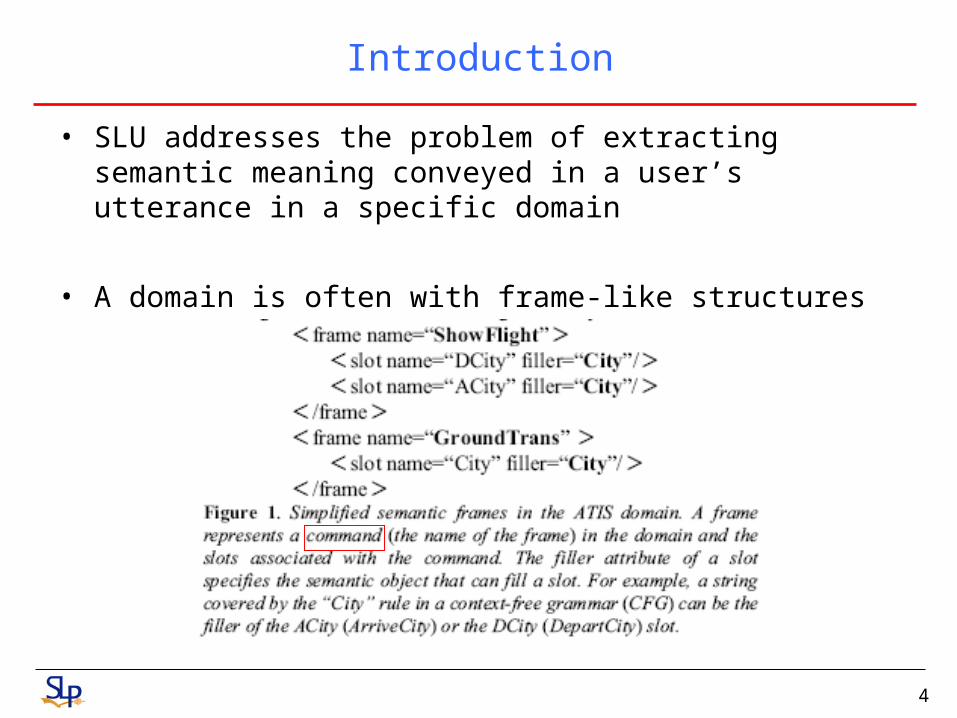
• SLU addresses the problem of extracting semantic meaning conveyed in a user’s utterance in a specific domain

• A domain is often with frame-like structures

5

Introduction

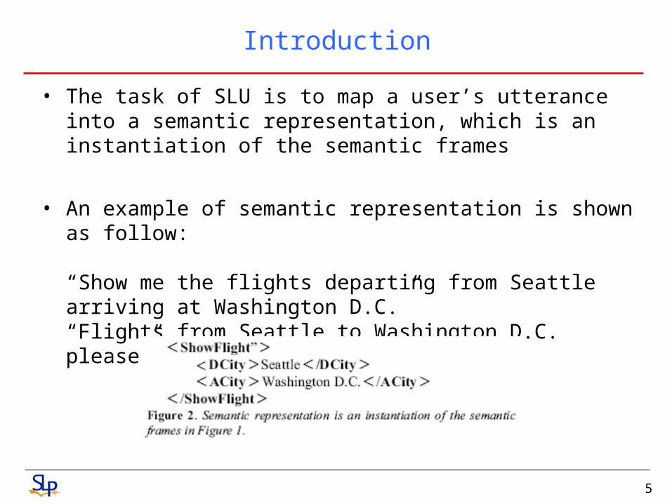
• The task of SLU is to map a user’s utterance into a semantic representation, which is an instantiation of the semantic frames

• An example of semantic representation is shown as follow: “Show me the flights departing from Seattle arriving at Washington D.C.” “Flights from Seattle to Washington D.C. please”

6

Introduction

• SLU is traditionally solved with a knowledge-based approach

• In the past decade many data-driven generative statistical models have been proposed for the problem

• Among them a HMM/CFG composite model integrates knowledge-based approach in a statistical learning framework, which uses CFG rules to define the slot fillers and HMM to disambiguate command and slots in an utterance

• The HMM/CFG composite model achieves the understanding accuracy at the same level as the best performing semantic parsing system based on a manually developed grammar in ATIS evaluation

7

Conditional models for SLU

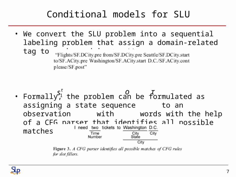
• We convert the SLU problem into a sequential labeling problem that assign a domain-related tag to each word in an utterance

• Formally, the problem can be formulated as assigning a state sequence to an observation with words with the help of a CFG parser that identifies all possible matches of CFG rules for slot fillers

τs1 o τ

8

Conditional models for SLU

• The model has to resolve several types of ambiguity:

• 1. Filler/non-filler ambiguity– e.g. “two” can be the filler of a NumOfTickets slot, or the preambl

e of the ACity slot

• 2. CFG ambiguity:– e.g. “Washington” can be CFG-covered as either a City or a State

• 3. Segmentation ambiguity:– e.g. “[Washington] [D.C.]” for two Cities v.s “[Washington D.C.]” r

epresents a single city

• 4. Semantic label ambiguity:– e.g. “Washington D.C.” can fill either “ACity” or a “DCity” slot

9

Conditional models for SLU

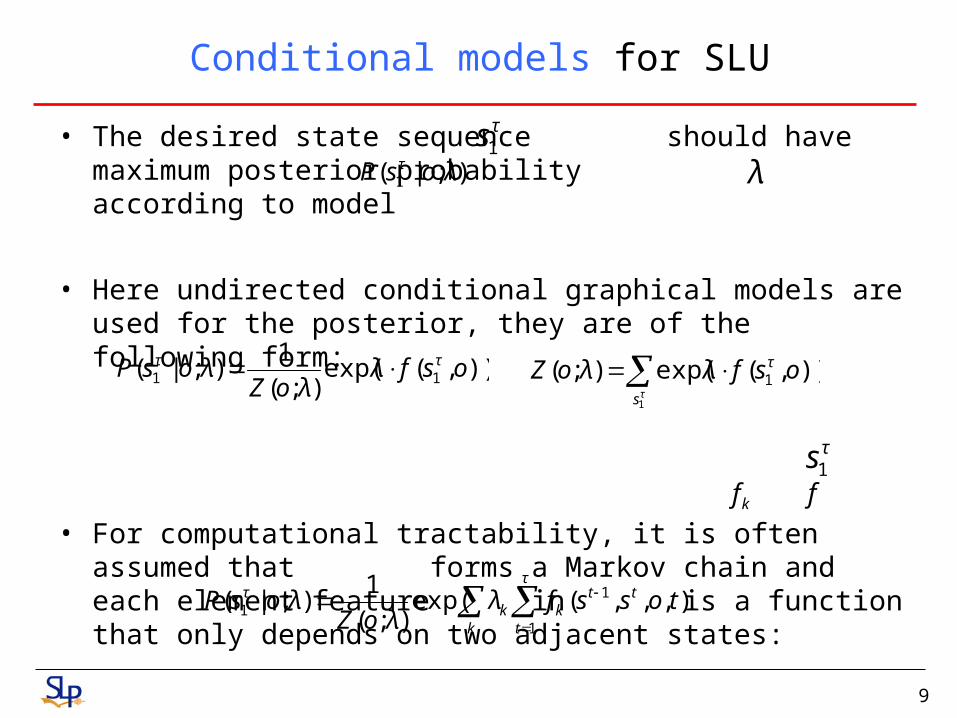
• The desired state sequence should have maximum posterior probability according to model

• Here undirected conditional graphical models are used for the posterior, they are of the following form:

• For computational tractability, it is often assumed that forms a Markov chain and each element feature in is a function that only depends on two adjacent states:

τs1);|( 1 λosP τ λ

)),(exp();(

1);|( 11 osfλ

λoZλosP ττ

τs

τ osfλλoZ1

)),(exp();( 1

τs1kf f

k

τ

t

ttkk

τ tossfλλoZ

λosP1

11 )),,,(exp(

);(

1);|(

10

Conditional models for SLU

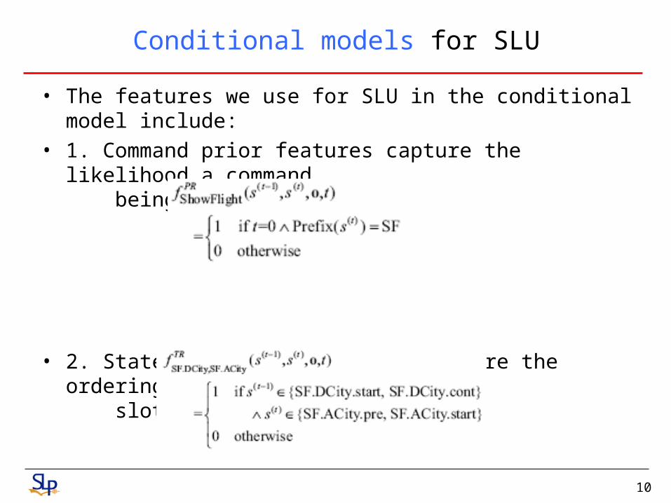
• The features we use for SLU in the conditional model include:

• 1. Command prior features capture the likelihood a command being issued by a user:

• 2. State transition features capture the ordering of different slot in a command:

11

Conditional models for SLU

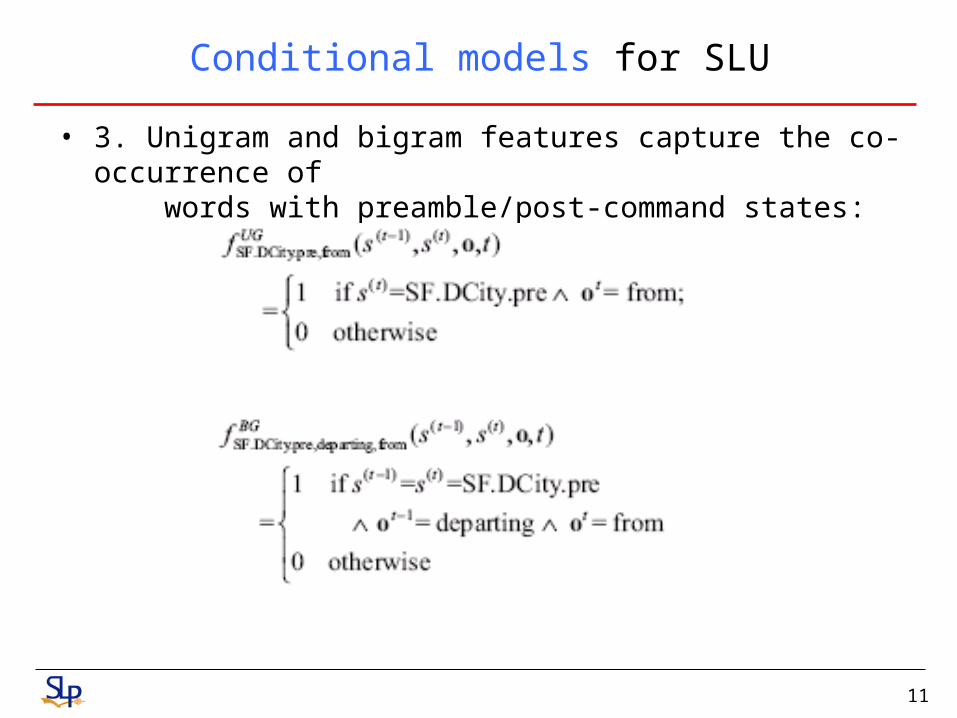
• 3. Unigram and bigram features capture the co-occurrence of words with preamble/post-command states:

12

Conditional models for SLU

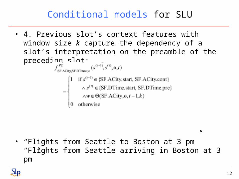
• 4. Previous slot’s context features with window size k capture the dependency of a slot’s interpretation on the preamble of the preceding slot:

• “Flights from Seattle to Boston at 3 pm”“Flights from Seattle arriving in Boston at 3 pm”

13

Conditional models for SLU

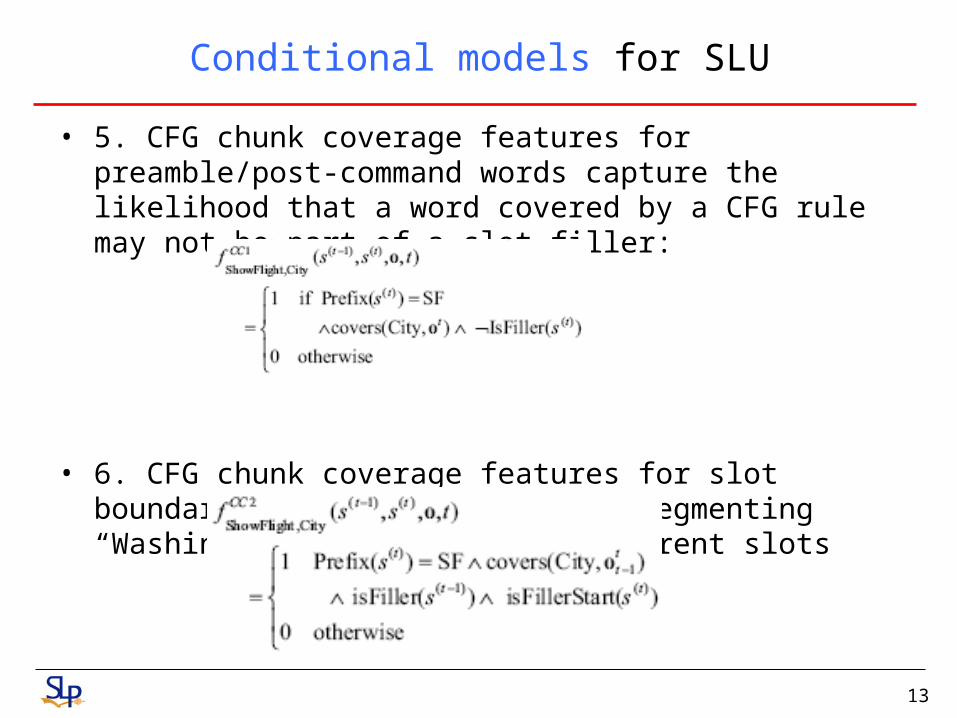
• 5. CFG chunk coverage features for preamble/post-command words capture the likelihood that a word covered by a CFG rule may not be part of a slot filler:

• 6. CFG chunk coverage features for slot boundaries prevent errors like segmenting “Washington D.C.” into two different slots

14

Discriminative Training – Conditional random fields

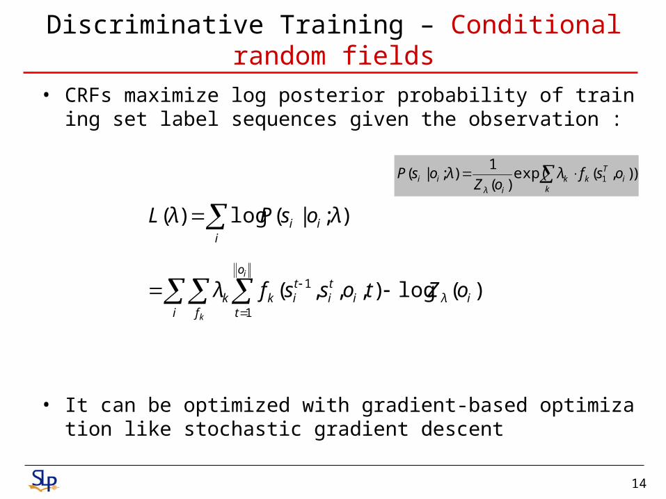
• CRFs maximize log posterior probability of training set label sequences given the observation :

• It can be optimized with gradient-based optimization like stochastic gradient descent

i fiλ

o

ti

ti

tikk

iii

k

i

oZtossfλ

λosPλL

)(log),,,(

);|(log)(

1

1

)),(exp()(

1);|( 1

ki

Tkk

iλii osfλ

oZλosP

15

Discriminative Training – Conditional random fields

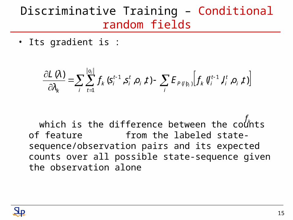
• Its gradient is :

which is the difference between the counts of feature from the labeled state-sequence/observation pairs and its expected counts over all possible state-sequence given the observation alone

ii

ti

tikolP

i

o

ti

ti

tik

k

tollfEtossfλ

λLi

i

),,,(),,,()( 1

)|(1

1

kf

16

Discriminative Training – Perceptron

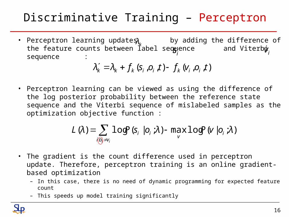
• Perceptron learning updates by adding the difference of the feature counts between label sequence and Viterbi sequence :

• Perceptron learning can be viewed as using the difference of the log posterior probability between the reference state sequence and the Viterbi sequence of mislabeled samples as the optimization objective function :

• The gradient is the count difference used in perceptron update. Therefore, perceptron training is an online gradient-based optimization

– In this case, there is no need of dynamic programming for expected feature count– This speeds up model training significantly

kλ

),,(),,( tovftosfλλ iikiikkk

is iv

ii voi

iv

ii λovPλosPλL:

);|(logmax);|(log)(

17

Discriminative Training – MCE

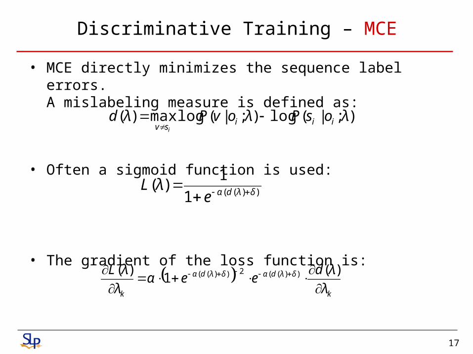
• MCE directly minimizes the sequence label errors. A mislabeling measure is defined as:

• Often a sigmoid function is used:

• The gradient of the loss function is:

))((1

1)(

δλdαeλL

);|(log);|(logmax)( λosPλovPλd iiisv i

k

δλdαδλdα

k λ

λdeeα

λ

λL

)(1

)( ))((2))((

18

Discriminative Training – MCE

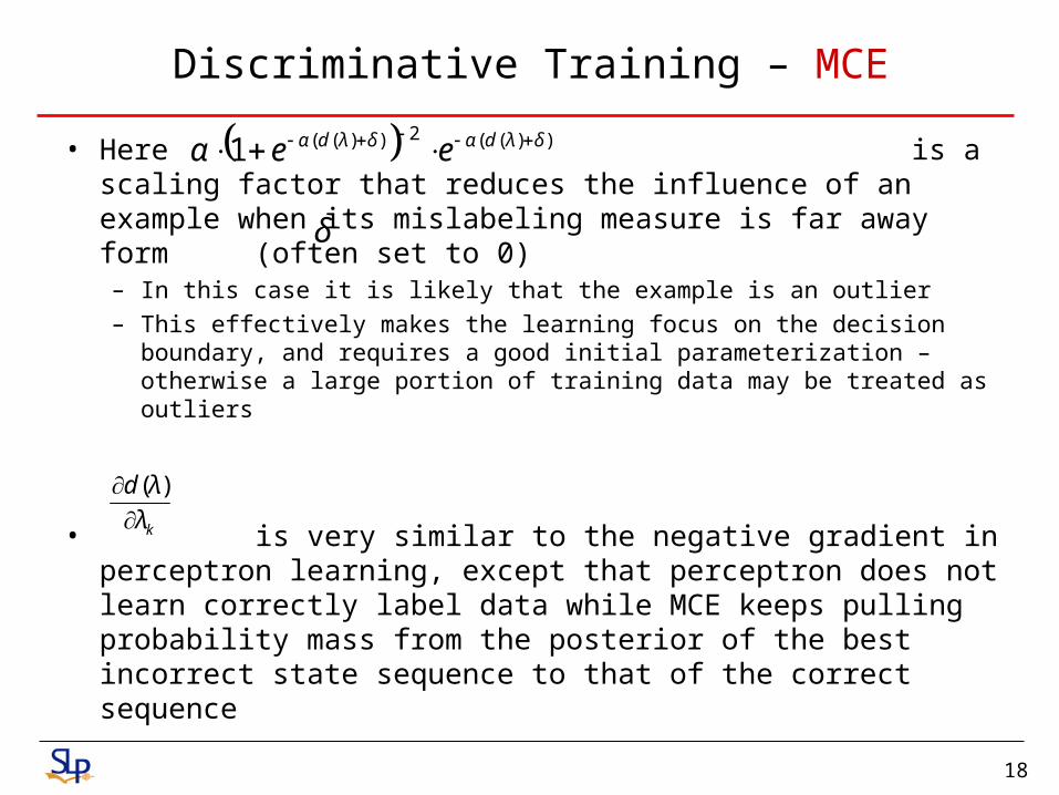
• Here is a scaling factor that reduces the influence of an example when its mislabeling measure is far away form (often set to 0) – In this case it is likely that the example is an outlier

– This effectively makes the learning focus on the decision boundary, and requires a good initial parameterization – otherwise a large portion of training data may be treated as outliers

• is very similar to the negative gradient in perceptron learning, except that perceptron does not learn correctly label data while MCE keeps pulling probability mass from the posterior of the best incorrect state sequence to that of the correct sequence

))((2))((1 δλdαδλdα eeα

δ

kλ

λd

)(

19

Discriminative Training – Large margin

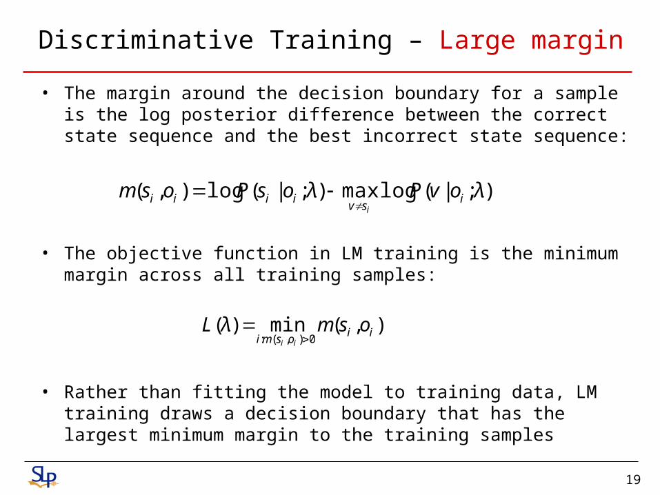
• The margin around the decision boundary for a sample is the log posterior difference between the correct state sequence and the best incorrect state sequence:

• The objective function in LM training is the minimum margin across all training samples:

• Rather than fitting the model to training data, LM training draws a decision boundary that has the largest minimum margin to the training samples

);|(logmax);|(log),( λovPλosPosm isv

iiiii

),(min)(0),(:

iiosmi

osmλLii

20

Discriminative Training – Large margin

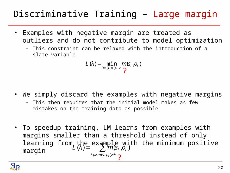
• Examples with negative margin are treated as outliers and do not contribute to model optimization

– This constraint can be relaxed with the introduction of a slate variable

• We simply discard the examples with negative margins– This then requires that the initial model makes as few mistakes on the training data

as possible

• To speedup training, LM learns from examples with margins smaller than a threshold instead of only learning from the example with the minimum positive margin

0),(:

),()(ii osmρi

ii osmλL

),(min)(),(:

iiεosmi

osmλLii

?

?

21

Corpus

• ATIS 3 category A– Training set (~1700 utterances)– 1993 test set (470 utterances , 1702 slots)– Development set (410 utterances)– Manually annotated for the experiments

22

Experimental Results – SLU accuracy

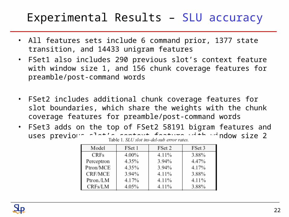
• All features sets include 6 command prior, 1377 state transition, and 14433 unigram features

• FSet1 also includes 290 previous slot’s context feature with window size 1, and 156 chunk coverage features for preamble/post-command words

• FSet2 includes additional chunk coverage features for slot boundaries, which share the weights with the chunk coverage features for preamble/post-command words

• FSet3 adds on the top of FSet2 58191 bigram features and uses previous slot’s context feature with window size 2

23

Experimental Results – Training speed

• Perceptron takes much fewer iterations and much less time per iteration than CRFs

• MCE converges faster than LM after perceptron initialization– This may due to the fact that all data participate in MCE training,

while only those with small positive margins participate in LM training

24

Experimental Results – Robustness to data sparseness

• CRFs and CRF-initialized MCE/LM models are more robust to data sparseness than perceptron and perceptron-initialized MCE/LM models

25

Conclusions

• We have introduced different discriminative training criteria for conditional models for SLU, and compared CRFs, perceptron, MCE and LM models in terms of accuracy, training speed and robustness to data sparseness

• Perceptron and perceptron-initialized MCE and LM models are much faster to train, and the accuracy gap becomes smaller when more data are available

• It is a good trade-off to use perceptron-initialized MCE or LM if training speed is crucial for an application, or a large amount of training data is available