DISCUSSION PAPER SERIES

DP14012 (v. 3)

FINANCE AND GREEN GROWTH

Ralph De Haas and Alexander Popov

FINANCIAL ECONOMICS

ISSN 0265-8003

FINANCE AND GREEN GROWTHRalph De Haas and Alexander Popov

Discussion Paper DP14012 First Published 19 September 2019

This Revision 07 January 2021

Centre for Economic Policy Research 33 Great Sutton Street, London EC1V 0DX, UK

Tel: +44 (0)20 7183 8801 www.cepr.org

This Discussion Paper is issued under the auspices of the Centre’s research programmes:

Financial Economics

Any opinions expressed here are those of the author(s) and not those of the Centre for EconomicPolicy Research. Research disseminated by CEPR may include views on policy, but the Centreitself takes no institutional policy positions.

The Centre for Economic Policy Research was established in 1983 as an educational charity, topromote independent analysis and public discussion of open economies and the relations amongthem. It is pluralist and non-partisan, bringing economic research to bear on the analysis ofmedium- and long-run policy questions.

These Discussion Papers often represent preliminary or incomplete work, circulated to encouragediscussion and comment. Citation and use of such a paper should take account of its provisionalcharacter.

Copyright: Ralph De Haas and Alexander Popov

FINANCE AND GREEN GROWTH

Abstract

We study how countries' financial structure affects their transition to low-carbon growth. Usingglobal industry-level data, we document that carbon-intensive industries reduce emissions faster ineconomies with deeper stock markets. Two channels underpin this stylized fact. First, stockmarkets reallocate investment towards energy-efficient sectors. Second, in countries with deeperstock markets, carbon-intensive sectors engage in more green innovation, resulting in lowercarbon emissions per unit of output. Only one-tenth of these industry-level reductions in domesticemissions are offset by carbon embedded in imports. A firm-level analysis of an exogenous shockto the cost of equity in Belgium confirms our findings.

JEL Classification: G10, O4, Q5

Keywords: Financial Development, Financial structure, Carbon Emissions, Innovation

Ralph De Haas - dehaasr@ebrd.comEBRD and CEPR

Alexander Popov - alexander.popov@ecb.intECB

AcknowledgementsWe thank Francesca Barbiero, Victoria Robinson, and Alexander Stepanov for outstanding research assistance and ThorstenBeck, Maurice Bun, Francesca Cornelli (discussant), Antoine Dechezlepretre, Kathrin de Greiff, Hans Degryse, Manthos Delis,Rodolphe Desbordes, Michael Ehrmann, Tim Eisert (discussant), Mara Faccio (discussant), Sergei Guriev, Florian Heider,Deborah Lucas, Mikael Homanen, Luc Laeven, Arik Levinson, Steven Ongena, Andrea Presbitero (discussant), Orkun Saka,Robert Sparrow (discussant), Vahap Uysal (discussant), Karen van der Wiel (discussant), and participants at the 8th DevelopmentEconomics Workshop (Wageningen University), 3rd CEPR Annual Spring Symposium in Financial Economics (Imperial College),12th Swiss Winter Conference on Financial Intermediation (Lenzerheide), Chicago Financial Institutions Conference, WesternFinance Association (WFA) Meeting, CEPR Conference on Financial Intermediation and Corporate Finance (Athens), and seminarsat the EBRD, University of New South Wales, University of Barcelona, Queen's University Belfast, Tinbergen Institute, CopenhagenBusiness School, London School of Economics, ECB, University of Bristol, Dutch Bureau for Economic Policy Analysis, IMF,Federal Reserve Board of Governors, Bank of England, De Nederlandsche Bank, Renmin University of China, Xiamen University,University of Sussex, University of Bonn, LSE Systemic Risk Centre, and the Humboldt University Climate-Finance webinar foruseful comments. The opinions expressed are the authors' and not necessarily those of the EBRD, the ECB, or the Eurosystem. Aprevious version of this paper circulated under the title \Finance and Carbon Emissions".

Powered by TCPDF (www.tcpdf.org)

Finance and Green Growth∗

Ralph De Haas†

EBRD, CEPR, and Tilburg University

Alexander PopovECB

Abstract

We study how countries’ financial structure affects their transition to low-carbongrowth. Using global industry-level data, we document that carbon-intensive indus-tries reduce emissions faster in economies with deeper stock markets. Two channelsunderpin this stylized fact. First, stock markets reallocate investment towards energy-efficient sectors. Second, in countries with deeper stock markets, carbon-intensivesectors engage in more green innovation, resulting in lower carbon emissions per unitof output. Only one-tenth of these industry-level reductions in domestic emissions areoffset by carbon embedded in imports. A firm-level analysis of an exogenous shock tothe cost of equity in Belgium confirms our findings.

JEL classification: G10, O4, Q5.

Keywords: Financial development, financial structure, carbon emissions, innovation

∗We thank Francesca Barbiero, Victoria Robinson, and Alexander Stepanov for outstanding research as-sistance and Thorsten Beck, Maurice Bun, Francesca Cornelli (discussant), Antoine Dechezlepretre, Kathrinde Greiff, Hans Degryse, Manthos Delis, Rodolphe Desbordes, Michael Ehrmann, Tim Eisert (discussant),Mara Faccio (discussant), Sergei Guriev, Florian Heider, Deborah Lucas, Mikael Homanen, Luc Laeven, ArikLevinson, Steven Ongena, Andrea Presbitero (discussant), Orkun Saka, Robert Sparrow (discussant), VahapUysal (discussant), Karen van der Wiel (discussant), and participants at the 8th Development EconomicsWorkshop (Wageningen University), 3rd CEPR Annual Spring Symposium in Financial Economics (Impe-rial College), 12th Swiss Winter Conference on Financial Intermediation (Lenzerheide), Chicago FinancialInstitutions Conference, Western Finance Association (WFA) Meeting, CEPR Conference on Financial In-termediation and Corporate Finance (Athens), and seminars at the EBRD, University of New South Wales,University of Barcelona, Queen’s University Belfast, Tinbergen Institute, Copenhagen Business School, Lon-don School of Economics, ECB, University of Bristol, Dutch Bureau for Economic Policy Analysis, IMF,Federal Reserve Board of Governors, Bank of England, De Nederlandsche Bank, Renmin University of China,Xiamen University, University of Sussex, University of Bonn, LSE Systemic Risk Centre, and the HumboldtUniversity Climate-Finance webinar for useful comments. The opinions expressed are the authors’ and notnecessarily those of the EBRD, the ECB, or the Eurosystem. A previous version of this paper circulatedunder the title “Finance and Carbon Emissions”.†Corresponding author. European Bank for Reconstruction and Development (EBRD), One Exchange

Square, EC2A 2JN, London, email: dehaasr@ebrd.com.

1 Introduction

The 2015 Paris Climate Conference (COP21) has put finance firmly at the heart of the debate

on climate change. The leaders of the G20 stated their intention to scale up green-finance

initiatives to fund low-carbon infrastructure and other climate solutions. Key examples

include the burgeoning market for green bonds, the establishment of the British Green

Investment Bank, and the creation of a green credit department by the largest bank in the

world—ICBC in China.

Somewhat paradoxically, the interest in green finance has also laid bare our limited

understanding of the relation between regular finance and the environment. To date, no

rigorous evidence exists on how finance affects industrial pollution as economies grow. Are

expanding banking sectors and stock markets detrimental to the environment as they fuel

economic growth and the concomitant emission of pollutants? Or can financial development

steer economies towards sustainable growth by favoring “green” sectors over “brown” ones?

A better understanding of the link between finance and pollution is important because most

of the global transition to a low-carbon economy will need to be funded by the private

financial sector if international climate goals are to be met on time (UNEP, 2011). Insights

into how banks and stock markets affect carbon emissions can also help policy makers to

benchmark the ability of special green-finance initiatives to cut emissions.

To analyze the channels that connect finance, industrial composition, and environmental

degradation—as measured by the emission of CO2—we exploit a 48-country, 16-industry, 26-

year panel.1 To preview our results, we first demonstrate that for given levels of economic and

financial development, CO2 emissions per capita are significantly lower in economies where

equity financing is more important relative to bank lending. Subsequent analysis at the

industry level shows that industries that pollute more for technological reasons, start to emit

relatively less carbon dioxide where and when stock markets expand. Our analysis reveals

two distinct channels that underpin these results. First—holding cross-industry differences

in technology constant—stock markets tend to reallocate investment towards more carbon-

efficient sectors. Second, stock markets facilitate the development of cleaner technologies by

1CO2 emissions are the main source of global warming as they account for over half of all radiative forcing(net solar retention) by the earth (IPCC, 1990; 2007). The monitoring and regulation of anthropogenic CO2

emissions is therefore at the core of international climate negotiations. CO2 emissions also proxy for otherair pollutants caused by fossil fuels such as methane, carbon monoxide, SO2, and nitrous oxides.

1

polluting industries. In particular, we show that deeper stock markets are associated with

more green patenting in carbon-intensive industries. This patenting effect is strongest for

inventions to increase the energy efficiency of industrial production. In line with this positive

role of stock markets for green innovation, our industry-level data show that carbon emissions

per unit of value added decline relatively more in carbon-intensive sectors in countries where

stock markets account for an increasing share of all corporate funding. Additional analysis

shows that neither the reallocation of investment towards more energy-efficient sectors nor

the increased energy efficiency in carbon-intense sectors are merely side effects of sectoral

variation in R&D-intensity or firms’ reliance on tangible assets.

The domestic green benefits of more developed stock markets may be offset by more

pollution abroad, for instance because equity-funded firms offshore the most carbon-intensive

parts of their production processes to foreign pollution havens. We show that the reduction

in emissions by carbon-intensive sectors due to domestic stock market development is indeed

accompanied by an increase in carbon embedded in imports of final and intermediary goods

of the same sector. This effect is stronger for ‘footloose’ industries that can more easily

outsource part of their production abroad. However, the domestic greening effect dominates

the pollution outsourcing effect by a factor of ten. This indicates that stock markets have

a genuine cleansing effect on polluting industries and do not simply help such industries to

shift carbon-intensive activities to pollution havens.

A concern in interpreting our industry-level panel evidence is the influence of omitted

factors that could confound the observed relation between the relative importance of stock

markets and the CO2 emissions of relatively polluting sectors. We deal with this issue in

three ways. First, and most importantly, we saturate our regressions with an exhaustive

set of interactive fixed effects (country-industry fixed effects as well as unobservable country

and industry trends). These fixed effects control for a host of potential confounding factors,

including general economic development and changes in environmental regulation. Second,

we employ policy shocks to both equity markets and banking sectors as instruments for the

size and structure of financial systems across countries and years. Third, we take advantage

of the fact that one of the countries in our sample, Belgium, introduced a notional interest

deduction (NID) for corporate equity in 2006. This policy shock provides an exogenous

source of variation to the cost of equity financing. Using firm-level data from Orbis and the

European Emissions Trading System (ETS), we trace how the NID reform caused Belgian

2

firms to increase their equity ratio (by about 5% of the sample mean) and to reduce the

carbon intensity of their production. Importantly, these results also hold in a difference-in-

differences setting where we compare the treated Belgian firms to a control group of firms in

the Netherlands (a neighboring country that did not reform its corporate tax law but was

exposed to similar economic shocks). The results also hold when we match Belgian firms to

observationally similar firms in the same 2-digit industry from a broader set of neighboring

countries and again apply a difference-in-differences framework.

This paper contributes to (and connects) three strands of the literature. First, we inform

the debate on economic growth and environmental pollution. Early work on this topic

focused on the environmental Kuznets hypothesis, according to which pollution increases at

early development stages but declines once a country surpasses a certain income level. Two

main mechanisms underlie this hypothesis. First, during the early stages of development, a

move from agriculture to manufacturing and heavy industry is associated with both higher

incomes and more pollution per capita. After some point, the economy moves towards

light industry and services, and this shift goes hand-in-hand with a leveling off or even a

reduction in pollution (Hettige, Lucas, and Wheeler, 1992 and Hettige, Mani, and Wheeler,

2000). Second, when economies develop, breakthroughs at the technological frontier (or

the adoption of technologies from more advanced countries) may substitute clean for dirty

technologies and reduce pollution per unit of value added (within a given sector).

While empirical work provides evidence for a Kuznets curve for a variety of pollutants,

the evidence for CO2 emissions is mixed.2 Schmalensee, Stoker, and Judson (1998) find an

inverse U-curve in the relationship between per capita GDP and CO2 emissions while Holtz-

Eakin and Selden (1995) show that CO2 emissions increase with per capita GDP but merely

stabilize when economies reach a certain income level. Our contribution is to explore the

role of finance in shaping the relation between economic growth and carbon emissions. In

particular, we assess how a country’s financial structure—the relative importance of stock

markets versus banks as corporate funding sources—affects the two main channels that

underpin the Kuznets hypothesis: a shift towards less-polluting sectors and an innovation-

driven reduction in pollution within sectors.

Second, a more recent literature views the link between growth and environmental pollu-

2Grossman and Krueger (1995) find a Kuznets curve for the pollution of urban air and river basins. SeeDasgupta, Laplante, Wang, and Wheeler (2002) for a literature review on the environmental Kuznets curve.

3

tion through the lens of endogenous growth theory (Aghion and Howitt, 1998). Acemoglu,

Aghion, Bursztyn, and Hemous (2012) and Acemoglu, Akcigit, Hanley, and Kerr (2016)

develop endogenous growth models with directed technical change. In these models, sus-

tainable growth depends on temporary carbon taxes and research subsidies that redirect

innovation towards clean technologies.3 A key macro parameter in these models is the elas-

ticity of substitution between clean (energy efficient) and dirty (carbon intense) production.4

Within a country, this substitution can reflect that industries become cleaner over time or

that resources shift towards sectors with a higher share of clean energy inputs. Our contri-

bution is to show how (changes in) the structure of a country’s financial system can shape

both these drivers of the elasticity of substitution between clean and dirty inputs.

Third, our results contribute to the literature on the relation between financial structure

and economic development. A substantial body of empirical evidence has by now estab-

lished that growing financial systems contribute to economic growth in a causal sense (King

and Levine, 1993).5 Earlier studies suggested that the structure of the financial system—

bank-based or market-based—matters little: both credit markets and stock markets con-

tribute positively to economic growth (Levine and Zervos, 1998; Beck and Levine, 2002;

Jerzmanowski, 2017). However, more recent research qualifies this finding by showing that

the impact of banking on growth declines (and the impact of stock markets increases) as

national income rises (Demirguc-Kunt, Feyen, and Levine, 2013; Gambacorta, Yang, and

Tsatsaronis, 2014), potentially explaining growth threshold effects in overbanked economies

(Arcand, Berkes, and Panizza, 2015). Our contribution is to show that the structure of the

financial system also matters for the degree of environmental degradation that accompanies

the process of economic development.

This paper is structured as follows. Section 2 discusses the link between financial struc-

ture and carbon emissions. Sections 3 and 4 then describe our empirical methodology and

data, respectively. Section 5 presents the empirical results and Section 6 concludes.

3Empirically, Aghion, Dechezlepretre, Hemous, Martin, and Van Reenen (2016) show how higher fuelprices redirect the car industry towards clean innovation (electric and hybrid technologies) and away fromdirty technology (internal combustion engines).

4Using industry-level data, Papageorgiou, Saam, and Schulte (2017) estimate that this elasticity is rela-tively high, at just below three, for the aggregate non-energy sector of the economy.

5For comprehensive surveys of this literature, see Levine (2005), Beck (2008), and Popov (2018).

4

2 Stock Markets, Banks, and Carbon Emissions

Financial structure, defined as the relative importance of equity versus credit markets, can

have an environmental impact if different forms of finance affect environmental pollution

to a different extent or through different channels. The existing literature suggests several

reasons why banks and stock markets may differentially affect industrial pollution.

On the banking side, three main arguments have been made. First, banks typically

operate with a relatively short horizon (the loan maturity) and may ignore whether funded

assets will become less valuable (or even stranded) in the more distant future. Ongena,

Delis, and de Greiff (2018) show how banks only recently started to price the climate risk

of lending to firms with large fossil fuel reserves. Anecdotal evidence also suggests that in

recent years banks became more sensitive to the financial and reputational risks associated

with lending to polluting firms (Zeller, 2010). Such a narrow focus on reputational risk

and environmental liability may of course not prevent banks with a short-term horizon from

lending to less visibly polluting industries, like those emitting large amounts of CO2.

Second, there is a large body of evidence indicating that bank lending (and debt funding

more generally) is ill-suited to finance innovative, high-risk–high-return projects. To the

extent that technological innovation is an important mechanism to contain environmental

pollution, this implies that banks may be relatively ineffective in reducing such pollution.

Several mechanisms can play a role. Banks may be technologically conservative: they fear

that funding new (and possibly cleaner) technologies erodes the value of collateral that

underlies existing loans that represent older (dirtier) technologies (Minetti, 2011). Banks

can also hesitate to finance green technologies if these involve assets that are intangible and

firm-specific (Hall and Lerner, 2010) and therefore difficult to collateralize (Carpenter and

Petersen, 2002). Asset intangibility and uncertainty are indeed characteristic of many energy

technology startups (Nanda, Younge, and Fleming, 2015). Lastly, banks may simply lack

the skills to assess early-stage (green) technologies (Ueda, 2004).6

Third, even if banks ignore environmental risk due to their short-term horizon (at least

until recently), and even if they are badly equipped to finance frontier innovation, their

lending may still alleviate firms’ financial constraints, including constraints that hold back

6In line with this skeptical view of banks as financiers of innovative technologies, Hsu, Tian, and Xu(2014) provide cross-country evidence that industries that depend on external finance and are high-techintensive are less likely to file patents in countries with more developed credit markets.

5

investment in pollution abatement. In line with this, Levine, Lin, Wang, and Xi (2018) show

how positive credit supply shocks in U.S. counties reduced local air pollution. In a similar

vein, Goetz (2019) finds that financially constrained firms reduced toxic emissions when their

capital cost decreased as a result of the U.S. Maturity Extension Program.

What about stock markets? First, mirroring the above arguments, equity may be better

suited to finance high-risk–high-return innovations, including new technologies to increase en-

ergy efficiency and reduce carbon emissions.7 Second, if equity investors care about (future)

pollution costs, then stock prices will rationally discount cash flows of polluting industries.

A key question is therefore to what extent investors take carbon emissions into account when

assessing longer-term corporate risk. Hart and Zingales (2017) develop a model predicting

that public firms, with their diffuse ownership and limited personal responsibility of each

voting investor, display an ‘amoral drift’ away from pro-social decisions, in contrast to closely

held private firms. In line with this, Shive and Forster (2020) find that private firms in the

U.S. emit fewer greenhouse gases as compared to otherwise similar public firms.

Yet, a growing body of evidence suggests that investors, especially institutional ones,

increasingly do take longer-term climate-change related risk into account and put pressure

on companies to reduce carbon emissions. Survey evidence by Krueger, Sautner, and Starks

(2020) shows that a large proportion of investment managers believe that climate risk is

already affecting their portfolio companies. Almost 40 percent of the surveyed investors

are therefore aiming to reduce the carbon footprint of their portfolios, including through

active engagement with management.8 Gibson Brandon and Krueger (2018) find that espe-

cially institutional investors with a longer-term horizon hold equity portfolios with a better

environmental footprint. Dyck et al. (2019) show likewise that institutional shareholder

ownership is positively and causally related to firms’ environmental and social performance.

Ormazabal et al. (2020) focus on the “Big Three” institutional investors (BlackRock, Van-

guard and State Street Global Advisors) and find a strong negative association between the

7Brown, Martinsson, and Petersen (2017) show that while credit markets foster growth in industries thatrely on external finance for physical capital accumulation, equity markets have a comparative advantage infinancing technology-led growth. In line with this, Kim and Weisbach (2008) find that most of the fundsthat firms raise in public stock issues are invested in R&D.

8Oil majors recently gave in to investor pressure to disclose the impact of climate policies on futureactivities (ExxonMobil) or to set carbon emissions targets (Royal Dutch Shell). Glencore, a coal miningcompany, announced that in response to investor demands it would cap coal production (Financial Times,2017; The Economist, 2018; Wall Street Journal, 2019).

6

ownership of equity by these investors, especially when they hold a significant stake, and

firms’ subsequent carbon emissions. Mutual funds and other institutional investors may also

benefit from pushing companies to reduce carbon emissions because this helps to attract en-

vironmentally responsible investment clients (Ceccarelli, Ramelli and Wagner, 2020). In line

with this, Hartzmark and Sussman (2019) show how a sudden increase in the transparency of

U.S. mutual funds’ sustainability ratings led to net inflows (outflows) into high-sustainability

(low-sustainability) funds.

Investor concerns about corporate exposure to climate-change risk is also affecting asset

prices and firms’ funding costs. Ilhan, Sautner, and Vilkov (2020) show for a sample of S&P

500 companies that higher emissions increase tail risk in put options and that this effect

is concentrated in high-emission industries. This suggests that stock market participants,

in particular institutional investors, take carbon emissions into account when assessing cor-

porate risk. Likewise, Bolton and Kacperczyk (2020) find that stocks of U.S. firms with

higher carbon emissions earn higher returns.9 Moreover, institutional investors appear to

shun carbon-intensive companies, although this effect is limited to direct emissions from

production and to the most carbon-intense industries.

In sum, whether banks or stock markets are better suited to reducing carbon emissions

remains an important open question. The aim of this paper is therefore to provide robust

empirical evidence—at the country, industry, and firm level—on the link between a country’s

financial structure and the amount of carbon dioxide that firms emit.

3 Empirical Methodology and Identification

We first estimate a regression to map financial sector trends into carbon emissions and where

countries are the unit of observation. In doing so, we distinguish between the size and the

structure of the financial system. We define financial sector size (or Financial Development,

FD) as the sum of private credit and stock market capitalization divided by the country’s

9Cheng, Ioannou, and Serafeim (2014) confirm for a cross-country sample of listed firms that increasedenvironmental responsibility improves firms’ access to finance. Chava (2014) shows how the environmentalprofile of a firm affects both the cost of its equity and its debt capital, suggesting that both banks andequity investors take environmental concerns into account. Higher capital costs can be an important channelthrough which investor concerns affect firm behavior and their pollution intensity. If higher capital costsoutweigh the cost of greening the production structure, firms will switch to a more expensive but less pollutingtechnology (Heinkel, Kraus, and Zechner, 2001).

7

gross domestic product:

FDc,t =Creditc,t + Stockc,t

GDPc,t

(1)

Next, we define Financial Structure (FS) as the share of stock market financing out of

total financing through credit and stock markets:

FSc,t =Stockc,t

Creditc,t + Stockc,t(2)

In both cases, Credit is the sum of credit extended to the private sector by deposit money

banks and other credit institutions while Stock is the value of all publicly traded shares.

With these proxies at hand, we proceed to estimate the following specification:

CO2c,t

Populationc,t

= β1FDc,t−1 + β2FSc,t−1 + β3Xc,t−1 + ϕc + φt + εc,t (3)

Here, CO2c,t

Populationc,tdenotes total per capita emissions of carbon dioxide in country c dur-

ing year t. Both Financial Development (FD) and Financial Structure (FS) are 1-period

lagged. Xc,t−1 is a vector of time-varying country-specific variables, such as the state of

environmental regulation, that can account for a sizeable portion of the variation in cross-

country CO2 emissions. Another important factor is economic development, the pollution

impact of which can be positive at early stages of development as the economy utilizes the

cheapest technologies available, and negative at later stages when the economy innovates to

reduce pollution (one of the environmental Kuznets-curve arguments). We account for this

by including the logarithm of per capita GDP, both on its own and squared. The phase of

the business cycle can also have an impact on pollution. For example, the economy may

cleanse itself from obsolete technologies during recessions.10 To account for this, we include

a dummy equal to 1 if the economy experiences negative growth.

10See Gali and Hammour (1991) and Caballero and Hammour (1994). Recessions may involve an envi-ronmental cleansing effect when inferior-technology companies are also the least energy efficient ones. Arecession will then prune these companies and improve the energy efficiency of the average (surviving) firm.Any such positive effects may be counterbalanced, however, if renewable energy investments are put on hold,thus delaying the introduction of cleaner technologies. Indeed, Campello, Graham, and Harvey (2010) showthat firms that were financially constrained during the global financial crisis cut spending on technology andcapital investments and bypassed attractive investment opportunities.

8

ϕc is a vector of country dummies that net out the independent impact on carbon emis-

sions of unobservable country-specific time-invariant influences, such as comparative advan-

tage or voters’ appetite for regulation. φt is a vector of year dummies that purge our estimates

from the effect of unobservable global trends common to all countries, such as the “Great

Moderation”, the adoption of a new technology across countries around the same time, or a

collapse in the demand for tradeables that reduces transportation intensity. Finally, εc,t is

an idiosyncratic error term. We cluster the standard errors by country to account for the

possibility that they are correlated within a country over time.

Interpreting the results from Model (3) as causal assumes that financial development is

unaffected by current or expected per capita carbon emissions, and that carbon intensity

and financial development are not affected by a common factor. The latter assumption is

questionable. For example, if global demand increases for products by carbon-intensive in-

dustries that rely on external finance, CO2 emissions and Financial Development increase

simultaneously without there necessarily being a causal link from finance to carbon emis-

sions. Alternatively, a reduction in income taxes can result simultaneously in higher stock

market investment and higher consumption, inducing a spurious positive correlation between

Financial Structure and carbon emissions. We address this point through a Two-Stage Least

Squares (2SLS) procedure in which policy changes induce exogenous shocks to financial sys-

tem size and structure. The first instrument measures pro-competitive bank regulation,

based on Abiad et al. (2008). It captures the degree to which domestic banking markets are

open to entry by foreign banks; open to entry by new domestic banks; open to branching

by existing banks; and open to the emergence of universal banks. The idea behind this

instrument is that bank liberalization should increase the size but reduce the equity share of

the financial system. The second instrument measures equity market liberalization (Bekaert

et al., 2005) and is a dummy equal to one in the years after equity markets open up to

investment by foreign investors. The idea is that opening up to foreign portfolio investment

should increase the equity share of the domestic financial system. Because both instruments

focus specifically on financial liberalization events, we expect the exclusion restriction to be

met as these shocks only influence carbon emissions through their impact on the size and/or

the structure of a country’s financial system.

Next, in the main part of our analysis, we estimate the impact of Financial Development

and Financial Structure on carbon emissions at the sector level. More specifically, we assess

9

the relative role of within-country financial development and financial structure for different

types of industries, depending on their technological propensity to emit carbon dioxide. The

working hypothesis is that shocks to the size and structure of financial systems impact dif-

ferentially per capita carbon emissions in carbon-intensive relative to carbon-light industries

in one and the same country. To test this hypothesis, we employ the following cross-country,

cross-industry regression framework:

CO2c,s,t

Populationc,t= β1FDc,t−1 × Carbon intensitys + β2FSc,t−1 × Carbon intensitys

+β3Xc,s,t−1 + ϕc,s + φc,t + θs,t + εc,s,t

(4)

Here, CO2c,s,t

Populationc,tdenotes total per capita emissions of carbon dioxide by industry s in

country c during year t.11 As in Model (3), FDc,t−1 is the sum of total bank credit to

the private sector and the total value of all listed shares, normalized by GDP, in country c

during year t− 1. FSc,t−1 is the total value of all listed shares, divided by the sum of total

credit to the private sector and the value of all listed shares, in country c during year t− 1.

Carbon intensitys is a time-invariant, sector-specific variable that measures the average

carbon dioxide emissions of sector s per unit of value added, in the global sample during

the sample period (see Table 1). The underlying assumption is that the global average of a

sector’s emissions per unit of value added captures the sector’s inherent propensity to pollute.

In robustness tests, we employ a proxy for Carbon intensitys that captures average carbon

dioxide emissions by the respective sector in the United States (over the sample period) and

another one based on the industry’s global average emissions in any given year.

In the most saturated version of Model (4), we control for Xc,s,t−1, a vector of interac-

tions between the industry benchmark for carbon intensity and time-varying country-specific

factors that capture economic development (GDP per capita), the size of the market (pop-

ulation), and the business cycle (whether the country is in a recession). This controls for

the possibility that the association between financial development and carbon emissions is

contaminated by concurrent developments in a country’s economy. Lastly, we saturate the

empirical specification with interactions of country and sector dummies (ϕc,s), interactions

of country and year dummies (φc,t), and interactions of sector and year dummies (θs,t). ϕc,s

11We express the industry-level carbon dioxide emissions in per capita terms to have uniform scalingacross countries; make the coefficients comparable to those in the country-level regressions; and to allow theindustry effects to sum up to aggregate effects.

10

nets out all variation that is specific to a sector in a country and does not change over

time (e.g., the comparative advantage of agriculture in France). φc,t eliminates the impact

of unobservable, time-varying factors that are common to all industries within a country

(e.g., voters’ demand for environmental protection). θs,t controls for all variation coming

from unobservable, time-varying factors that are specific to an industry and common to all

countries (e.g., technological development in air transport).12

In the next two steps, we test for the channels via which financial systems exert an im-

pact on carbon emissions. The first channel is one whereby—holding technology constant—

financial markets (or some types thereof) reallocate investment away from technologically

carbon-intensive towards technologically ‘green’ industries. This channel manifests itself if

energy-efficient sectors grow relatively faster in countries dominated by either banks or stock

markets. The second channel is one whereby—holding the industrial structure constant—

some forms of finance are better at improving the energy efficiency of technologically ‘dirty’

industries, bringing them closer to their technological frontier. This channel will result in

carbon-intensive sectors becoming greener over time in countries dominated by either banks

or stock markets.

We test for the presence of the first channel using the following regression model:

∆V alue addedc,s,t = β1FDc,t−1 × Carbon intensitys + β2FSc,t−1 × Carbon intensitys+β3Xc,s,t−1 + ϕc,s + φc,t + θs,t + εc,s,t

(5)

where relative to Model (4), the only change is that the dependent variable is now the

percentage change in value added between year t − 1 and year t by industry s in country

c. The evolution of this variable over time measures the industry’s growth relative to other

industries in the country. It can therefore capture the degree of reallocation that takes

place in the economy from technologically carbon-intensive towards technologically green

12Institutional investors may avoid carbon-intensive sectors (Bolton and Kacperczyk, 2020). Any variationin institutional ownership at the sector-country and year-country level will be absorbed by our fixed effects.Yet, institutional ownership at the country-sector level may also evolve over time and this change may becorrelated with our main independent variable of interest, the interaction between financial structure anda sector’s carbon intensity. We do not disentangle this potential role of changes in institutional ownershipin stock markets (at the country-year-sector level) from the more general impact of changes in financialstructure, but acknowledge that this is a potentially important mechanism through which stock marketdevelopment can affect sectoral carbon emissions.

11

industries. Earlier work has shown how well-developed stock and credit markets make coun-

tries more responsive to global common shocks by allowing firms to better take advantage of

time-varying sectoral growth opportunities (Fisman and Love, 2007). Evidence also suggests

that financially developed countries increase investment more (less) in growing (declining)

industries (Wurgler, 2000).

We test for the presence of the second mechanism using the following regression model:

CO2c,s,t

V alue addedc,s,t= β1FDc,t−1 × Carbon intensitys + β2FSc,t−1 × Carbon intensitys

+β3Xc,s,t−1 + ϕc,s + φc,t + θs,t + εc,s,t

(6)

where relative to Model (4), the only change is that the dependent variable is now the

total emissions of carbon dioxide by industry s in country c during year t, divided by the

total value added of industry s in country c during year t. The evolution of this variable

over time thus measures the change in an industry’s energy efficiency—that is, how dirty the

production process is per unit of value added.

Lastly, to gauge whether improvements in carbon efficiency over time are due to own

innovation (as opposed to technological adoption), we evaluate the following model:

Patentsc,s,tPopulationc,t

= β1FDc,t−1 × Carbon intensitys + β2FSc,t−1 × Carbon intensitys+β3Xc,s,t−1 + ϕc,s + φc,t + θs,t + εc,s,t

(7)

The dependent variable is one of several measures of green patent production, in industry

s in country c during year t, divided by the population in country c in year t. These variables

capture the propensity of industries to engage in green innovation. This propensity may be

stronger in carbon-intensive industries as well as in countries with a more developed financial

system or one dominated by a particular type of finance.

4 Data

This section introduces the four main data sources we use. We first describe the data

on carbon emissions, then the industry-level data on value added and green patents, and

finally the country-level data on financial development. We also discuss the matching of the

industry-level data. Appendix Table A1 contains variable definitions and data sources.

12

4.1 CO2 emissions

We obtain data on CO2 emissions from fuel combustion at the sectoral level from the Inter-

national Energy Agency (IEA).13 The original data set contains information for 137 countries

over the period 1974–2015. Information on CO2 emissions is reported both at the aggregate

level and for a total of 16 industrial sectors, which are based on NACE Rev. 1.1. These

sectors encompass each country’s entire economy, and not just the manufacturing sector,

which is important given that some of the main CO2-polluting activities, such as energy

supply and land transportation, are of a non-manufacturing nature. The 16 sectors are: (1)

Agriculture, hunting, forestry, and fishing; (2) Mining and quarrying; (3) Food products,

beverages, and tobacco; (4) Textiles, textile products, leather, and footwear; (5) Wood and

products of wood and cork; (6) Pulp, paper, paper products, printing, and publishing; (7)

Chemical, rubber, plastics, and fuel products; (8) Other non-metallic mineral products; (9)

Basic metals; (10) Fabricated metal products, machinery, and equipment; (11) Transport

equipment; (12) Electricity, gas, and water supply; (13) Construction; (14) Land transport

– transport via pipelines; (15) Water transport; and (16) Air transport.

We next produce a data set of countries that each have a fair representation of industries

with non-missing CO2 data. We drop countries that have fewer than half of the sectors with

at least 10 years of CO2 emissions data. This results in a final data set of 48 countries with

at least 8 sectors with at least 10 years of CO2 emissions data. We combine the country-level

and the industry-level data on CO2 emissions with data on each country’s population, which

allows us to construct the dependent variables in Models (3), (4), and (7).

4.2 Industry value added

To calculate the dependent variables in Models (5) and (6), we need industry data on value

added. We obtain these from two sources. The first one is the United Nations Industrial

Development Organization (UNIDO) data set, which contains data on value added in manu-

facturing (21 industries) for all countries in the IEA data set. The second one is the OECD’s

STAN Database for Structural Analysis which provides data on value added for all sectors

in the economy, but it only covers the 28 OECD countries in our final data set. We can

therefore calculate proxies for CO2 emissions per unit of value added, for value added growth,

1380% of anthropogenic CO2 emissions are due to the combustion of fossil fuels (Pepper et al., 1992).

13

and for each sector’s share of total output in the country, for two separate data sets. One

contains all 48 countries with data on CO2, as well as all manufacturing sectors, while the

other comprises 28 of the 48 countries, as well as all sectors in the economy. The main tests

in the paper are based on the former data set with a view to maximizing country coverage,

but we also include tests based on the latter data set to maximize sector coverage. We

winsorize the data on value added growth at a maximum of 100% growth and decline. To

make value added by the same industry comparable across countries, we convert all nominal

output into US$ and then deflate it to create a time series of real industrial output.

4.3 Green patents

To evaluate Model (7), we use the largest international patent database—the Patent Statis-

tical database (PATSTAT) of the European Patent Office (EPO)—to calculate the number

of green patents across countries, sectors, and years. Because of an average delay in data

processing in PATSTAT of 3.5 years, our patent data end in 2015. We follow the method-

ological guidelines of the OECD Patent Statistics Manual and take the year of the priority

filing as the reference year. If a patent does not have a priority filling, the reference year is

the year of the application filling. This ensures that we closely track the timing of inventive

performance. We take the country of residence of the inventor as the reference country. If a

patent has multiple inventors from different countries, we use fractional counts: each country

is attributed a corresponding share of the patent. Every patent indicator is based on data

from a single patent office and we use the United States as the primary patent office.14

PATSTAT classifies each patent according to the International Patent Classification

(IPC). We round this classification to 4-character IPC codes and use the concordance table

of Lybbert and Zolas (2014) to convert these codes into ISIC 2-digit sectors.15 We then

use these data to construct three patenting variables. The first one, ‘Green patents’, counts

all patents granted to a particular country, sector, and year and that belong to the EPO

14In unreported robustness checks, we calculate patent indicators using the EPO as the primary office.The correlation coefficients between the US and European indicators range between 0.75 and 0.81.

15PATSTAT also classifies patents according to NACE 2. A drawback of this classification is that it onlycovers manufacturing. Given that our scope is broader, we do not use this as our baseline approach but onlyin robustness checks. To ensure comparability between both approaches, we convert NACE 2 into ISIC 3.1.The correlation coefficients between both indicator types vary between 0.93 and 0.98.

14

Y02/Y04S climate change mitigation technology (CCMT) tagging scheme.16 CCMTs include

all technological inventions to reduce the amount of greenhouse gas emitted when produc-

ing or consuming energy. The scheme is the most reliable method for identifying green

patents and has become the standard in studies on green innovation (Popp, 2019). The

second variable, ‘Green patents (excluding transportation and waste)’, counts all granted

CCMT patents except for those with the tag Y02T (Climate change mitigation technologies

related to transportation) or Y02W (Climate change mitigation technologies related to solid

and liquid waste treatment). The third variable, ‘Green patents (industrial production)’,

only counts CCMT patents that belong to the arguably most important category of patents

(Y02P) for our purposes: patents related to inventions to increase the energy efficiency of

the industrial production or processing of goods.

4.4 Country-level data

Our measures of financial system size and structure, FD and FS, are calculated using two

country-specific data series. The first one is the value of total credit by financial intermedi-

aries to the private sector (lines 22d and 42d in the IMF International Financial Statistics)

normalized by GDP. These data exclude credit by central banks, credit to the public sec-

tor, and cross claims of one group of intermediaries on another. They count credit from all

financial institutions rather than only deposit money banks. The data come from Beck et

al. (2016) and are available for all countries in the data set.17 The second country-specific

data series is the value of all stocks, normalized by GDP. This is a measure of the total value

of traded stock, not of the intensity with which trading occurs. These data too come from

Beck et al. (2016) and are available for all countries as well. The correlation between FD

and FS in the sample is 0.19, suggesting that while the two variables are not excessively

correlated, it is important to study their impact on carbon emissions simultaneously

Chart 1 plots the annual sample average of FD and FS between 1974 and 2015. During

these four decades, the overall size of financial systems more than tripled (relative to gross

domestic product). Chart 1 also shows that the relative importance of stock markets more

16We disregard empty sector-year-country cells, so that we effectively focus on the intensive margin ofgreen innovation.

17In unreported tests, we document that the results of the paper go through (and are indeed statisticallystronger) if we only use the corporate-lending segment of private credit, for those countries for which thesedata are available.

15

than doubled during this period. That is, stock markets tend to catch up with credit markets

at later stages of development. One issue is that both data series are patchy before 1990,

especially for Central and Eastern European countries. We therefore drop these observations

so that our final data set comprises 48 countries observed between 1990 and 2015.18

We also use data on real per capita GDP, population, and recessions (defined as an

instance of negative GDP growth) from the World Development Indicators. Lastly, we use the

OECD Environmental Policy Stringency Index (EPS), a country-specific and internationally

comparable measure of the stringency of environmental policy. It captures the degree to

which environmental policies put an explicit or implicit price on polluting or environmentally

harmful behavior and ranges between 0 (not stringent) and 6 (very stringent).19

4.5 Concordance and summary statistics

Our data are available in different industrial classifications. The original IEA data on carbon

dioxide emissions are classified across 16 industrial sectors, using IEA’s classification. The

UNIDO and STAN data on value added are classified in 2-digit industrial classes using the

ISIC classification. This calls for a concordance procedure to match the disaggregated ISIC

sectors with the broader IEA sectors. The matching results in a total of 16 industrial sectors

with data on both carbon dioxide emissions and industrial output. While some sectors

are uniquely matched between IEA and UNIDO/STAN, others result from the merging of

ISIC classes. For example, ISIC 15 “Food products and beverages” and ISIC 16 “Tobacco

products” are merged into ISIC 15–16 “Food products, beverages, and tobacco”, to be

matched to the corresponding IEA industry class.

Appendix Table A2 summarizes the data. At the country level, we use aggregate CO2

emissions (in metric tons), divided by population. The average country emits 6.78 metric

tons of CO2 per capita each year. The financial variables show that in the average country,

the sum of private credit and stock market capitalization exceeds gross domestic product.

However, there is a large dispersion, with FD as small as 0.03 in Azerbaijan in 1999, and

as large as 4.16 in Switzerland in 2007. The same holds for FS: while the share of stock

markets in the total financial system is on average 0.39, it is only one-tenth of a percent in

Bulgaria in 1997, but 0.82 in Finland in 2000. The data on GDP per capita indicate that the

18See Online Appendix Table OA1 for a list of these countries.19See Botta and Kozluk (2014) for more details.

16

data set contains a good mix of developing countries, emerging markets, and industrialized

economies. The median country has a GDP per capita of $14,051 and a population of 14.4

million. On average, a country is in a recession once every five years.

The industry-level data from UNIDO show that the median industry emits 0.071 metric

tons of carbon dioxide per capita per year, and 0.269 metric ton per US$ thousand of value

added. Over the sample period, the median industry grows by 0.1% per year and makes

up about 0.6% of total manufacturing. These values are relatively consistent across the

UNIDO and STAN data sets. However, the median STAN industry records larger per capita

emissions than the median UNIDO industry because the four heaviest polluters—ISIC 40 and

41 “Electricity, gas, and water supply,” ISIC 60 “Land transport – transport via pipelines,”

ISIC 61 “Water transport,” and ISIC 62 “Air transport”—are not manufacturing industries.

In terms of green patents, the average country-industry produces around 0.2 such patents

per 1 million people in both samples.

Table 1 presents the concordance key to map 62 ISIC classes into 16 IEA ones, including

9 manufacturing sectors. It also summarizes, by sector, our main industrial benchmark,

‘Carbon intensity’, calculated as the average emissions of carbon dioxide per unit of value

added by all firms in the respective sector across the world and over the whole sample period.

5 Empirical Results

This section investigates the relation between finance and carbon emissions at the country

level (Section 5.1), industry level (Section 5.2), and firm-level (Section 5.3). Section 5.4

presents robustness tests.

5.1 Finance and pollution: Aggregate results

Table 2 reports results, using aggregate data, on the link between finance and carbon emis-

sions. We estimate three versions of Model (3). The first one is an OLS model on the full

sample. The second one applies OLS to a sample of 28 OECD countries, so that we can

control for environmental regulation. Third, we run a 2SLS model on the full sample, using

banking liberalization and equity-market liberalization events as instruments. Because not

all data are available for each country-year, the number of observations is reduced to at most

17

1,074 (out of a possible 1,248).

In column (1), we regress per capita carbon emissions on FD and FS, the other country

controls, and country and year dummies. We fail to reject the null hypothesis that financial

system size is uncorrelated with per capita carbon emissions. At the same time, controlling

for the size of financial systems, per capita carbon emissions are lower in countries where

firms get more of their funding from stock markets. The point estimate is significant at the

5% level. Column (2) uses the sub-sample of 28 OECD countries, so that we can control for

the stringency of environmental regulation. The same pattern obtains in the data. While

the overall size of financial systems is not associated with carbon emissions, when we control

for this size, more equity-based economies emit fewer carbon emissions per capita. The data

also confirm that more stringent environmental regulation is significantly and negatively

correlated with aggregate per capita emissions, all else equal.

In both regressions, we account for the fact that financial development correlates with

general economic development, and so the former may pick up the effect of higher incomes

on the demand for pollution. We therefore add GDP per capita and the square thereof. In

the full sample, the Kuznetz-curve effect survives controlling for financial system size and

structure: per capita CO2 emissions increase and then decrease with economic development.

The specification indicates that carbon emissions start declining at an annual income of

around $65,463 which is the 95th percentile in our country-level income distribution.

We include two other controls, both of which have the expected sign. First, more populous

countries emit fewer carbon emissions per capita, suggesting a negative pollution premium to

market size. Second, recessions are associated with lower per capita CO2 emissions. There

are two explanations for this. First, output declines during a recession, reducing overall

pollution too. Second, firms may use downturns to purge themselves from obsolete (and

more carbon-intensive) technologies (Caballero and Hammour, 1994).

We next move to our 2SLS results. Columns (3) and (4) report the first-stage. Both

instruments are significantly correlated with financial sector size and structure. By making

it easier for banks to enter and branch out, bank liberalization events increase the size

of financial systems. By allowing inward portfolio investment, equity market liberalization

events increase the share of equity financing. The relation with the overall size of the financial

system is negative, suggesting that equity liberalization tends to slow down banking sector

growth (controlling for the strictness of bank regulation). The first-stage Wald statistics,

18

reported as F -statistics, are consistent with the critical value for the IV regression to have

no more than 10% of the bias of the OLS estimate (Stock and Yogo, 2005).

Column (5) provides the second-stage 2SLS results. Even when inducing exogenous

shocks to FD and FS, the earlier patterns hold. Financial development on its own is uncor-

related with carbon emissions. But, importantly, for a given level of financial and economic

development, a country’s economy generates fewer carbon emissions per capita if it receives

more of its funding from stock markets. The absolute value of the point estimate increases

substantially in the 2SLS model, which suggests that unobservable factors that correlate

positively with the equity share of overall finance also do so with per capita emissions.

Numerically, the point estimate in column (5) suggests that increasing the share of equity

financing by 1 percentage point, while holding the size of the financial system constant,

reduces aggregate per capita carbon emissions by 0.077 metric tons. What are the aggregate

implications of this? We note that for several countries that are not financial centers and

have large banking sectors, such as Australia, Canada, Finland, and the Netherlands, FS

is approximately 0.5 throughout the sample period. Suppose that we take all countries

below this threshold and lift them to FS = 0.5, and we leave every country with FS > 0.5

unchanged. For about 80% of the countries in the data set, this would imply an average

increase in FS of 0.2 (from an average of around 0.3). Doing so would reduce per capita

pollution by around 1.54 metric tons. Given average per capita emissions of 6.8 (Appendix

Table A2), this would reduce current aggregate per capita emissions by about 22.6%. This

is more than half of the 40% reduction in emissions that countries committed to achieve by

2030 in the context of the Paris Agreement.

5.2 Finance and pollution: Industry-level results

5.2.1 Per capita carbon emissions

We next turn to sector-level data. We start by constructing a proxy for each industry’s

natural propensity to pollute that is exogenous to pollution in each particular industry-

country. Our main proxy is industry-specific average CO2 emissions per unit of value added,

calculated across all countries and years in the sample (Table 1). The assumption is that a

long-term global average better reflects the technological capabilities of an industry than its

performance in an individual country. In later robustness tests, we allow this benchmark to

19

change over time to account for the possibility that the technological frontier evolves. We

also take inspiration from Rajan and Zingales (1998) and calculate each industry’s average

CO2 emissions per unit of value added in the United States. The assumption in this case

is that an industry’s pollution intensity in a country with few regulatory impediments and

with deep and liquid financial markets reflects its inherent propensity to pollute.

In Table 3, we evaluate Model (4) to test whether the difference in carbon emissions by

technologically more versus less carbon-intensive sectors becomes smaller in countries with

financial systems that expand and/or become more skewed towards equity. Crucially, all

regressions in Table 3 (and thereafter) are saturated with country-sector dummies, country-

year dummies, and sector-year dummies. This ensures that the statistical associations we

measure in the data are not contaminated by unobservable factors that are specific to a sector

in a country and that do not change over time; by unobservable time-varying factors that

are common to all industries within a country; and to unobservable, time-varying factors

that are specific to an industry and common to all countries. We cluster standard errors at

the country-sector level.

Table 3 confirms the findings from the aggregate tests in Table 2. Column (1) shows that

carbon-intensive sectors do not generate relatively higher CO2 emissions per capita in coun-

tries with growing financial sectors. However, in column (2) we find that carbon-intensive

sectors produce relatively fewer per capita CO2 emissions in countries with relatively rapidly

expanding stock markets. This effect is significant at the 5% statistical level. We also note

that sectors that produce a larger share of overall value added, pollute more per capita than

smaller sectors.

These patterns hold when we include FD and FS together in column (3). Overall

financial sector size again does not matter for CO2 emissions. Yet, controlling for financial

development, an increase in the equity dependence of an economy generates a larger decline

in CO2 emissions in carbon-intensive industries. Column (4) reruns the specification in the

preceding column while accounting for the potential endogeneity in financial sector size and

structure. We again use the indices of banking liberalization and equity market liberalization

events to induce exogenous variation in the two main characteristics—size and structure—of

the financial system.

The results in column (4) strongly suggest that our earlier findings are not driven by

reverse causality whereby trends in carbon emissions increase an economy’s relative use of

20

equity finance, or by omitted variable bias whereby an unobservable factor causes a simulta-

neous decline in carbon emissions and an increase in the equity reliance of the economy. We

continue to find that in countries with expanding equity markets (relative to banking sec-

tors) carbon-intensive sectors generate fewer carbon emissions per capita. This relationship

is economically meaningful too. Take a country at the 25th percentile of FS (Germany) and

one at the 75th percentile (Australia). The interaction coefficient of pollution intensity and

FS in column (4) (−0.0925) means that giving Australia’s financial structure to Germany,

while keeping the size of its financial system constant, would reduce CO2 emissions by 0.14

metric tons in the most relative to the least polluting industry.

5.2.2 Channels

Our main finding so far is that per capita carbon emissions decline—more so in technolog-

ically carbon-intensive sectors—as the relative importance of equity funding grows. This

raises the question via which channels equity translates into lower carbon emissions? There

are two main potential channels. The first one is cross-industry reallocation whereby—

holding technology constant—stock markets reallocate investment towards greener sectors.

The second one is within-industry technological innovation whereby—holding industrial

structure constant—industries develop and implement greener technologies when access to

equity improves. We now test whether any of the two, or both, channels are operational.

Cross-industry reallocation. In Table 4, we test for the first channel using Model (5).

The dependent variable is the growth in value added in an industry in a particular country

and year. All regressions are again saturated with country-sector dummies, country-year

dummies, and sector-year dummies. A negative coefficient on the interaction term of interest

would imply that financial development reallocates investment away from carbon-intensive

sectors. This test is conceptually similar to Wurgler (2000) who finds that in countries with

deeper financial systems, investment is higher in booming than in declining sectors.

Column (1) shows that technologically carbon-intensive sectors do not grow at a different

rate, relative to greener sectors, in countries with larger financial systems. In column (2),

we find that carbon-intensive sectors grow more slowly (or, conversely, that green industries

grow faster) in countries with expanding stock markets. This effect is significant at the 10%

statistical level. We document the same patterns when we control for the size and structure

21

of financial systems jointly (column (3)) and when using IV instead of OLS (column (4)).

According to all specifications, larger sectors grow more slowly, a result in line with theories

of growth convergence.

We conclude that our evidence supports the conjecture that—holding cross-sector differ-

ences in technology constant—stock markets promote a reallocation of investment towards

greener (in the carbon-emissions sense) sectors. This partially explains the negative associ-

ation between financial structure and industry-level CO2 emissions per capita (Table 3).

Within-industry efficiency improvement. In Table 5, we test the second channel by

estimating Model (6). The dependent variable is sector-level annual CO2 emissions per unit

of value added and, once again, all regressions are saturated with country-sector dummies,

country-year dummies, and sector-year dummies. In this case, a negative coefficient on the

interaction term of interest would imply that financial development results in a technolog-

ical improvement within an environmentally dirty industry, regardless of its level of overall

growth. Yet, column (1) returns no evidence that within-sector carbon efficiency is affected

by changes in the size of the financial system. This aligns with our previous evidence where

we found no statistical association between the size of a country’s financial system and per

capita carbon emissions in relatively polluting versus green sectors.

We next look at the independent role of financial structure for carbon emissions per unit

of value added. Column (2) indicates that stock market development plays an important

role in within-sector efficiency. In particular, carbon emissions per unit of value added de-

cline relatively more in carbon-intensive sectors, in countries where stock market funding

accounts for an increasing share of overall funding (holding overall funding constant). This

effect is significant at the 1% statistical level. This pattern also obtains when we include the

size and structure of financial systems simultaneously (column (3)) and when we account

for the potential endogeneity in financial sector size and structure (column (4)). Indeed,

the absolute value of the point estimate increases relative to the OLS case, indicating that

unobservable factors that correlate positively with the equity share of overall finance also

correlate positively with carbon intensity. CO2 emissions per unit of value added would

decrease significantly if a country was to convert some of its bank funding into equity financ-

ing. Going back to our earlier thought experiment, the interaction coefficient of pollution

intensity and FS (−9.36) indicates that giving Germany (a country at the 25th percentile

22

of FS) the financial structure of Australia (at the 75th percentile of FS), while keeping the

size of its financial system constant, would reduce CO2 emissions by 2.8 metric tons per US$

1 million of value added in the most, relative to the least, polluting industry.

Table 5 suggests that stock markets facilitate the development and/or adoption of greener

technologies in carbon-intensive sectors. This evidence thus helps explain the role that stock

markets play in reducing per capita carbon emissions over time, as documented in Table 3.

5.2.3 Finance and green innovation

We find that CO2 emissions per unit of value added decline with stock market development,

especially in carbon-intensive industries. An intuitive interpretation is that this reflects the

propensity of carbon-intensive industries to become more carbon-efficient in countries where

more financing comes from equity markets. Such an effect could come from two directions:

either companies adopt already existing green technology20 or they develop such technologies

from scratch.21 We now provide direct evidence for the latter conjecture by using data on

industrial patenting (see Section 4.3) to estimate Model (7). We report OLS and 2SLS

results in Panels A and B of Table 6 and again test for the role of FD and FS jointly.

Both panels indicate that carbon-intensive sectors do not have a different propensity

to patent green technologies (compared with greener sectors) in countries with deepening

financial systems. This holds for all three green patent definitions. However, we do find that

the number of green patents increases faster in carbon-intensive sectors in countries with

deepening stock markets (column (1) in both panels). We find the same when excluding

green patents related to transportation and waste (column (2) in both panels). Strikingly,

when we focus on the ‘greenest’ patents, those intended to increase energy efficiency in

the production or processing of goods, we again find that an increasing share of equity

funding is strongly associated with an increase in these patents. This effect is significant at

the 1% level (column (3) in both panels) and is economically meaningful, too. The 2SLS

20Schumpeterian growth models suggest that financial constraints may prevent firms in less-developedcountries from exploiting R&D carried out in countries closer to the technological frontier (Aghion, Howitt,and Mayer-Foulkes, 2005).

21Howell (2017) shows that firms that receive grant funding from the U.S. Small Business Innovation Re-search Program generate more revenue and patent more (compared with similar but unsuccessful applicants).These effects are largest for financially constrained firms and those in sectors related to clean energy andenergy efficiency.

23

coefficient of 0.6024 in column (3) of Panel B indicates that moving from the 25th to the 75th

percentile of financial structure is associated with an increase in green patents generated by

an industry at the 75th percentile of carbon intensity—relative to one at the 25th percentile

of pollution intensity—of 0.14 patents per million (three times the sample mean). These

results complement those of Hsu, Tian and Xu (2014), who show that industries relying on

external finance and are high-tech intensive are more (less) likely to file patents in countries

with deeper equity (credit) markets. We show that stock markets also play an important

role in enabling carbon-intensive industries to make their production processes more energy

efficient through green innovation.22

5.2.4 OECD sample

One may query whether our results are driven by a particular sample choice. Our find-

ings so far are based on the UNIDO sample which features more countries (48) but fewer

sectors (9 manufacturing ones).23 The UNIDO sample contains many developing countries

and emerging markets and may thus produce empirical regularities that are driven by the

manufacturing industry in countries with relatively low economic and financial development.

We now replicate our main tests in the OECD sample, using data from STAN. This allows

us to run our tests on a sample of fewer countries (28) but more sectors (16), encompassing

the whole economy with the exception of services. This is potentially important because

the heaviest polluters in terms of carbon emissions per unit of value added are not part of

manufacturing (Table 1). Including them ensures that our results are not driven by a special

relationship between finance and carbon emissions in the manufacturing sector.

With this strategy in hand, we replicate the most saturated versions of Models (4)–(6),

the ones with country-sector dummies, country-year dummies, and sector-year dummies—in

the OECD sample. Table 7 reports OLS and 2SLS results in the odd and even columns,

respectively. We still find that deeper stock markets are associated with a reduction in per

22Financial development could also affect industry-level pollution through within-industry shifts acrossproducts with different pollution intensities. Shapiro and Walker (2018) show that such within-industryreallocation has not been a significant driver of the sharp reduction in US manufacturing pollution since the1990s. Instead, this reduction mainly reflects lower pollution per unit of value added within narrowly definedproduct categories. Our results are in line with this and highlight the role of stock markets in enabling greeninnovation.

23It is worth noting that together with primary industry, the manufacturing sector accounts for almost40% of worldwide greenhouse gas emissions (Martin, de Preux, and Wagner, 2014).

24

capita pollution levels (columns (1) and (2)) and that this result is fully driven by an increase

in within-industry efficiency (columns (5) and (6)). We do not find a differential impact of

deeper stock markets on growth in carbon-intensive versus greener sectors (columns (3) and

(4)). Table 7 thus suggests that the negative relationship between stock market development

and carbon emissions is by and large not a feature of a sample dominated by lower-income

countries or by economies at early stages of financial development.

5.2.5 Mechanisms

Our results so far raise a natural question about the deeper mechanisms at play. They suggest

that financial structure affects aggregate carbon emissions via two distinct channels. When

financial systems become more skewed towards equity markets, green sectors grow relatively

faster and, second, carbon-intensive sectors become more energy efficient, partly due to

increased green innovation and patenting. What are the deeper economic forces underpinning

these two channels? There is no ex-ante theory about why financial systems—or segments

thereof—should affect directly the relative performance of carbon-intensive sectors. At the

same time, there are a number of theories that could explain our results even in the absence

of such a direct effect.

One possibility is that energy-efficient sectors are more innovation intensive than carbon-

intensive sectors, and stock markets tend to be better at funding innovation than banks (Kim

and Weisbach, 2008; Brown, Martinsson, and Petersen, 2017). For example, as discussed

in Section 2, banks may lack the skills to evaluate early-stage technologies (Ueda, 2004) or

operate with a time horizon that is incompatible with the funding of long-term R&D. If

this is the case, then controlling for a sector’s propensity to innovate could explain away the

statistical association between financial structure and a reallocation from carbon-intensive

towards more energy-efficient sectors.

Another possibility is that carbon-intensive firms own more tangible assets while energy-

efficient firms depend more on intangible assets. Banks may then refuse to finance green

projects because intangible assets are hard to collateralize (Carpenter and Petersen, 2002;

Hall and Lerner, 2010). Equity markets, on the other hand, may be better suited to finance

green firms with intangible assets. If this mechanism is driving our results, then a sector’s

asset tangibility is another factor that can explain the statistical association between financial

structure and reallocation towards relatively energy-efficient sectors.

25

Third, it is possible that stock markets dominate banks in ways that are related more

directly to climate risk. In particular, environmental disasters expose firms to potential

litigation costs, which is why stock markets tend to be more sensitive to the financing of

firms that perform badly in environmental terms (Klassen and McLaughlin, 1996). Large-

scale ecological accidents, such as the Bhopal disaster or the Exxon Valdez oil spill, are

associated with severe litigation risk (Salinger, 1992). When it comes to future litigation

risk, shareholders have skin in the game while creditors are exempt. As a consequence,

equity investors may have an incentive to either stay away from carbon-intensive sectors or,

conditional on investing in them, to push for a ‘greening’ of their production technologies in

order to reduce future litigation risk. If this is the case, then controlling for the likelihood

of future litigation could moot the association between financial structure and the energy-

efficiency improvement in carbon-intensive sectors.

To test for whether these mechanisms are at play, we augment our principal regression

framework with the interaction of FD and FS with three alternative industry benchmarks.

The first one is R&D intensity. In the spirit of Rajan and Zingales (1998), this proxy takes

the industry-median value of R&D investment over total assets, for large mature companies

in Compustat (data come from Laeven, Klapper, and Rajan, 2006). The second benchmark

is Asset tangibility, measured as the ratio of an industry’s tangible assets to total assets (the

data, also derived from large mature companies, come from Braun, 2003). The third bench-

mark is Litigation risk. This variable is constructed as the total environmental penalties

and fines paid by a sector in the U.S. over the period 2000–2014 (following both administra-

tive and judicial legal cases) divided by the sector’s value added over the same period. The

penalty data come from the Environmental Protection Agency (EPA)’s Enforcement and

Compliance History Online (ECHO) data set. Online Appendix Table A10 reports industry-

level correlations between carbon intensity, R&D intensity, asset tangibility, and litigation

risk (Table 1 provides sector averages). The statistics suggest that all of the mechanisms dis-

cussed above could be at play. Carbon-intensive sectors are less R&D-intensive (correlation

of -0.37), more asset-tangible (0.40), and also more litigation-prone (0.75).

We investigate the empirical relevance of these mechanisms in Table 8 and do so separately

for the two channels at play: between-sector reallocation and within-sector improvements in

energy efficiency. In Panel A, we test for the possibility that the relative expansion of green

sectors in countries with deepening stock markets is explained by such sectors being more

26

R&D-intensive, less asset-tangible, and less litigation-prone. We augment Model (5) with

interactions of FD and FS with the three benchmarks just discussed, introducing them one

by one. Odd (even) columns present our OLS (IV) results.

We find that, as expected, R&D-intensive sectors grow faster in countries with deepening

stock markets (columns (1) and (2)). We also find that sectors rich in tangible assets expand

faster in economies that rely more on bank financing (columns (3) and (4)). These results

are entirely in line with the intuition discussed. Importantly, in both cases the impact of

financial structure on growth in energy-efficient relative to carbon-intensive sectors remains

in the 2SLS specifications and even becomes stronger (columns (2) and (4)). This suggests

that the reallocation of investment towards relatively energy-efficient sectors in countries

with deepening stock markets is not merely a side effect of these sectors also being more

innovative and less rich in tangible assets. At the same time, we find that litigation risk does

not explain cross-sector reallocation (columns (5) and (6)).

In Panel B, we test whether carbon-intensive sectors also being less R&D-intensive, more

asset-tangible, and more litigation-prone, explains the increase in energy efficiency in such

sectors in countries with deepening stock markets. We do not find that carbon emissions per

unit of value added decline relatively more in R&D-intensive sectors as stock markets develop

(columns (1) and (2)). The same is true when we control for the possibility that equity-

markets induce innovation in asset-intangible sectors (columns (3) and (4)). At the same

time, across all four specifications we again continue to find that stock market development

leads to a cleaning of carbon-intense industries relative to more energy-efficient ones.

Importantly, stock-market deepening also reduces carbon emissions per unit of value

added in litigation-prone sectors in the 2SLS specification (column (6)). Moreover, this

weakens somewhat the statistical association between financial structure and the reduction

in the gap in energy efficiency between relatively polluting and relatively clean sectors. The

technological ‘greening’ of carbon-intensive sectors as stock markets develop is therefore

to some degree also explained by equity investors being concerned about litigation risk.

These results go in the same direction as a number of recent findings in the literature. In

particular, Fernando, Sharfman, and Uysal (2017) find that institutional investors tend to

avoid stocks with high environmental risk exposure, while Akey and Appel (2020) show that

increased liability protection leads to higher toxic emissions as a result of lower investment

in abatement technologies. At the same time, even in this regression, financial structure

27

continues to be strongly and negatively correlated with carbon emissions per unit of value

added in carbon-intensive sectors. We therefore conclude that neither R&D-intensity, asset

tangibility, nor litigation risk can fully explain the results documented earlier in Table 5.

Our findings thus leave a role for alternative mechanisms that are more difficult to test, such

as individual investors having different social objectives than banks, for example.

5.2.6 Finance, imports, and carbon leakage

An important issue to address is that the decline in domestic carbon emissions due to stock

market development might be offset by the outsourcing of carbon-intensive activities to other

countries, including so-called pollution havens (Eskeland and Harrison, 2003; Aichele and

Felbermayr, 2015). This would result in a concomitant increase in carbon embedded in

imports of intermediate inputs or final consumer goods. Stock market funding is ultimately

provided by investors with their own social objectives (Bolton, Li, Ravina, and Rosenthal,

2020) and investors may be more sensitive to firms that perform badly in environmental

terms. One unintended consequence may be that firms close domestic operations, but open

foreign ones, under the assumption that poor environmental performance away from home

is more acceptable (or less observable) to investors. If so, then the decline in pollution

domestically would be neutralized by a proportionate increase in pollution elsewhere (carbon

leakage), making for a null effect from a global point of view.24

To test this hypothesis, we download detailed data from the World Input-Output Database

on bilateral imports and exports. We then calculate the amount of carbon emissions em-

bedded in the import of goods for each country-sector-year in the following way. First, we

determine what shares of output in a country-sector-year is exported versus sold domesti-

cally, and we split the associated CO2 proportionately. We then determine what share of

total exports by a particular sector in country i was imported by country j, and we assign

to country j a proportionate share of the overall CO2 associated with these exports. Next,

we sum over all WIOD countries i that export to country j to get the full amount of CO2

associated with the import in country j of goods (of a particular sector) produced abroad.

24A related concern is that stock market development involves substantial within-country cross-sectorspillovers through, for example, purchased materials and outsourced activities (so-called scope 3 emissions).While addressing the role of upstream and downstream spillovers is beyond the scope of this paper, we areless concerned about such indirect emissions because of the clear negative aggregate relationship betweenfinancial structure and country-level emissions shown in Table 2.

28

We also determine the final user in country j of these imported goods, and assign each

a proportionate share of the associated CO2 emissions abroad. There are five final-user

categories: households; the same sector; other sectors; gross fixed capital formation (GFCF);

and the government. In the case of the same sector and other sectors, these are typically

purchases of intermediate inputs—for instance, purchases of car parts produced in Indonesia

for the production of cars in Germany. In the case of households and the government, these

are typically purchases of final goods (e.g., cars). Lastly, in the case of GFCF, these are

(for example) cars and car parts imported by German firms to be used as investment goods

rather than intermediate inputs. For each of these categories, we calculate per capita carbon

emissions, to make the analysis comparable to Table 3.

Previous evidence suggests that outsourcing to pollution havens may be particularly likely

for ‘footloose’ sectors with a lower cost of relocating operations abroad (Ederington, Levin-

son, and Minier, 2005). This suggests that carbon emissions associated with the production

of imported goods will be higher in such footloose sectors. We acquire data from Ederington,

Levinson, and Minier (2005) on the costs of relocating production abroad, and aggregate it

to match our sector classification.25 The combination of these new data allows us to test

whether in countries with a growing share of equity financing, carbon embedded in imports

increases in case of carbon-intensive sectors, especially if the industry can relatively easily

outsource (parts of) its production.

Table 9 reports estimates from a modified Model (4) where the dependent variable is per

capita CO2 emissions associated with the production of imported goods (in total and for

the five user categories). Column (1) shows that in countries where equity markets gain in

relative importance, imports from carbon-intensive sectors go up. This means that part of

the decline in domestic carbon emissions due to increased equity financing is neutralized by

an increase in carbon emitted during the production of imports. However, the magnitude

of the point estimate is one-half of the one in Table 3, column (3), and overall imports are

only around one-fifth of domestic production. The increase in carbon emissions associated

with the production of imported goods is therefore only around one-tenth of the reduction in

domestic carbon emissions due to the relative growth of equity markets. The analysis across

25We classify sectors by their product market transportation costs. Industries where such costs are highare less likely to relocate abroad because the distance between production and consumers is then too costlyto overcome. The classification is based on industry fixed effect coefficients from a regression of transportcosts on distance and distance squared. See Appendix A of Ederington et al. (2005) for details.

29

final users reveals further interesting patterns. Goods purchased by households account

for around 5% of the overall increase in CO2 embedded in imported goods (column (2)).

Intermediate goods purchased by the same sector (column (3)) and by other sectors (column

(4)) account for the remaining 95%, in a roughly equal proportion. There is no increase in

carbon embedded in imports of either capital goods (GFCF) or government purchases.

In Online Appendix Table OA2, we distinguish between sectors for which production is

difficult to outsource due to high transportation costs (Panel A) and sectors that can out-

source more easily (Panel B). As expected, the overall effect on carbon emissions associated

with the foreign production of imported goods is much stronger for footloose sectors (Panel

B, column (1)) than for immobile ones (Panel A, column (1)). That is, when stock market

development leads to a domestic reduction in per capita carbon emissions in a relatively

polluting industry, then this greening effect is offset more (but still far from completely) in

the case of sectors whose products can be easily sourced abroad.

Interestingly, the import of consumer goods and of intermediates play intuitively different

roles. The relatively small contribution of households to the increase in carbon emissions

abroad that we documented for the full sample in Table 9 is much stronger for relatively

immobile industries (Panel A, column (2)). Instead, the contribution of outsourcing by

domestic industrial sectors is much stronger in the case of relatively footloose industries

(Panel B, columns (3) and (4)). These results are consistent with the idea that the more

footloose a sector is, the more it outsources the production of intermediary goods abroad.

For immobile sectors we instead observe that a domestic greening is accompanied by an

increase in households buying final consumer goods abroad (as well as some firms buying

investment goods abroad, column (5) in Panel A).

Overall, our estimates indicate that the reduction in carbon emissions in carbon-intensive

sectors due to domestic stock market development is accompanied by an increased reliance

of these sectors on the production of intermediary goods abroad (and to a much smaller

extent an increase in household consumption of imports). This holds in particular for more

footloose sectors. Yet, in terms of magnitudes, the increase in carbon embedded in sectoral

imports remains dominated by a greening of the domestic economy by a factor of ten. In all,

our findings are therefore in line with Levinson (2009) and Shapiro and Walker (2018) who

show that the cleanup of US manufacturing since the late 1980s mainly reflects technological

progress and only to a very limited extent the shifting of polluting industries overseas.

30

5.3 Finance and pollution: Firm-level results

We have not yet documented the link between the type of finance used and environmental

performance at the firm level. To support the evidence on the within-industry greening

effect of stock markets, it must be the case that when firms move towards more equity

financing, they tend to invest more in pollution-reducing technologies and generate fewer

carbon emissions per unit of value added. Demonstrating this chain of events is difficult

because firms’ choice of funding sources is typically endogenous, making the causal link from

equity to lower carbon emissions tenuous.

To address this issue, we use a new firm-level data set and a plausibly exogenous policy

change that reduced the cost of equity funding to firms. Specifically, we exploit the 2006

introduction of a tax shield for equity in Belgium that allowed firms to deduct from their

taxable income an interest calculated on the basis of their equity. This notional interest

deduction (NID) or allowance for corporate equity (ACE) reduced the relative tax advantage

of debt funding and made equity funding relatively cheaper for firms.26 Existing evidence

indicates that this policy change indeed significantly increased the share of equity in Belgian

firms’ funding structure (Schepens, 2016 and Hebous and Ruf, 2017).

We use a sample of Belgian non-financial corporations that we observe before and after

the introduction of the NID. We collect information on all Belgian firms that report annual

emissions under the EU Emissions Trading System (ETS). More specifically, we use firm-

level data on metric tons of carbon dioxide equivalent, which describes for a given mixture

and amount of emitted greenhouse gas, the amount of CO2 that would have the same global

warming potential. From Orbis we obtain data to calculate annual equity ratios, defined

as shareholder funds as a percentage of total current plus non-current liabilities. We have

non-missing information on both emissions and financials for 159 Belgian firms.

We compare these Belgian firms to two control groups. First, we use 101 ETS-reporting

Dutch corporations. The Netherlands is a neighboring country with a similar economy and

history27, but it did not introduce a tax shield on equity in 2006 or later. This control group

helps ensure that we do not capture a global (or regional) move toward more equity funding

26The NID allows firms to deduct from their taxable income a notional charge that equals the product ofthe book value of equity and a benchmark interest rate (the 10-year government bond yield). The BelgianNID is “hard” in the sense that the allowance is calculated over the total book value of equity instead ofnewly issued equity only (as in a “soft” NID).

27Both countries were part of the United Kingdom of the Netherlands until 1839.

31

unrelated to the Belgian reform.

Second, we use as a control group all ETS-reporting firms in the Netherlands, France,

Germany and Luxembourg. These are all of Belgium’s neighboring countries, closely eco-

nomically integrated and sharing the same currency. This larger control group allows us to

match each treated Belgian firm with a similar control firm before applying our difference-in-

difference estimator (Heckman, Hidehiko, and Todd, 1997). We match strictly within 2-digit

industries and further refine the match using nearest-neighbor propensity score matching.

The following variables enter the propensity score model: tangibility (tangible assets/total

assets); profitability (EBITDA/total assets); size (log of total assets); and a dummy for neg-

ative operating revenues. All firm characteristics refer to 2004, two years before the Belgian

reform came into force.

With these data in hand, we can answer two questions. First, did Belgian firms use more

equity after the introduction of the NID in 2006? And second, did Belgian firms reduce their

carbon emissions after 2006 and, if so, did they do so relative to control firms in neighboring

countries? To answer these questions, we first compare the panel of Belgian firms before and

after the introduction of the NID. In a second step, we then compare their development with

that of both control groups in a difference-in-differences framework. To mimic our previous

analysis, we calculate sector-specific carbon intensities as the median carbon emissions by

sales or by assets for all 33 countries for which firm-level CO2 data are available from the

ETS. We do this for all 24 sectors available in Orbis. The regressions include firm fixed

effects, as well as year fixed effects where appropriate.

We report the results in Table 10. Column (1) of Panel A documents a significant increase

in the share of equity funding after the introduction of the NID, confirming the existing

literature.28 On average, after 2006, Belgian firms used 0.64 percentage points more equity

(an increase of 5% of the sample mean). This increase in the share of equity in firms’ capital

structure is significant at the 5% statistical level. Columns (2) and (3) further indicate that

after 2006, Belgian firms in relatively polluting industries experienced a reduction in their

carbon equivalent emissions per sales and per assets, respectively. Both effects are significant

at the 1% statistical level, and represent a 20% reduction in the difference in emissions

28The observation period for columns (1) in all three panels is a symmetric window 1995–2018 aroundthe 2006 NID introduction in Belgium. For columns (2)-(3) a shorter period is used (2005–2018) since ETSreporting on carbon emissions only started in 2005.

32

between an industry at the 25th and one at the 75th percentile of emissions intensity.

Panel B provides difference-in-differences results using the Dutch ETS-reporting firms

as controls. We find that as a result of the NID introduction, Belgian firms became less

leveraged over time, also when compared to Dutch neighboring firms (column (1)). While

the data indicate a downward trend in firm leverage in the Netherlands as well, the post-2006

drop in leverage among Belgian firms is about 60% larger. The results in columns (2) and (3)

confirm that after 2006, Belgian firms in relatively polluting industries reduced their carbon

equivalent emissions per sales and per assets, also when compared to Dutch firms.

Panel C reports difference-in-differences results using matched firms from all neighboring

countries as a control group. The results are striking in that they show how Belgian firms

significantly increased their use of equity after 2006, also when compared to observationally

similar firms in adjacent countries (column (1)). Moreover, while the carbon intensity of ETS

firms in relatively polluting industries in these comparison countries increased post-2006, this

increase is much smaller among the Belgian firms (columns (2)-(3)).29

In short, the results in Table 10 confirm at the firm-level what we documented at the

industry level: a higher reliance on equity funding, due to an exogenous shift in firms’ incen-

tives to fund themselves with equity, results in fewer carbon equivalent emissions, plausibly

due to the implementation of greener technologies.

5.4 Robustness tests

One potential concern with our empirical specification is that we assume that the impact

of shocks to financial sector size and structure is relatively contemporaneous (1-year lag).

Changes in overall financing and in the equity share thereof may nevertheless take more time

to fully propagate through the economy. To account for this, we now impose a structure

that aggregates the data over 5-year periods (1990–1993, 1994–1998, 1999–2003, 2004–2008,

2009–2013). We then test for the impact of shocks to financial sectors during one 5-year pe-

riod on carbon emissions and sector growth during the next 5-year period. Online Appendix

Table OA3 reports the estimates from these alternative tests. The specifications control for

the time-varying size of each sector as a share of the economy and for country-sector dum-

mies, country-period dummies, and sector-period dummies. We find strong support for the

29Results are robust to clustering the standard errors at either the firm or the country level.

33

three stylized facts that we already documented: in countries with deepening stock markets,

and relative to technologically greener industries, carbon-intensive industries generate fewer

carbon emissions per capita (column (1)), grow more slowly (column (2)), and generate fewer

emissions per unit of value added (column (3)). These effects are statistically significant at

least at the 10% level, and at least at the 5% level in two of the three tests.

In Online Appendix Table OA4 we include both components of FD—the volume of bank

credit and the value of traded stocks—separately in the regression. Column (1) suggests that

an increase in stock market size a negative effect on CO2 emissions at the industry level. The

latter is driven by a reduction in relative growth rates in carbon-intensive sectors (column

(2)) and by a reduction in carbon emissions per unit of value added in carbon-intensive

sectors (column (3)), confirming the main results of the paper.

Next, our baseline results in Tables 3–5 are confirmed when we control for how dependent

on external finance a sector is (Online Appendix Table OA5) and when we employ alternative

benchmarks for carbon intensity, calculated using US data or contemporaneous sector-specific

global averages (Online Appendix Table OA6). Furthermore, we document that our main

results hold up well when we include the depth of corporate bond markets (Online Appendix

Table OA7) or the size of private equity investment (Online Appendix Table OA8) in the

calculation of FD and FS. The latter likely reflects that private equity, such as venture

capital and angel investments, is often instrumental for generating early-stage innovation

(Kortum and Lerner, 2000). Lastly, the main results also survive when we control for

country-industry-specific fuel subsidies (Online Appendix Table OA9). Fuel subsidies may

blunt firms’ incentives to make their production technology more energy efficient, even when

firms can access stock markets to finance such green investments.

6 Conclusions

The 2018 Sveriges Riksbank Nobel Prize in Economic Sciences was awarded to William

Nordhaus for integrating climate change into long-run macroeconomic analysis. Economists,

both theorists and empiricists, are increasingly analyzing the interdependent relationships

between economic growth and global warming. As yet, many questions remain unanswered

and economic research lags behind the proliferation of climate policies. The rapid growth of

green finance initiatives is a case in point and contrasts sharply with the paucity of evidence

34

on the link between conventional finance and carbon emissions.

To quantify this role, we study the relation between financial development and structure,

on the one hand, and CO2 emissions, on the other hand, in a large panel of countries and

sectors over the period 1990–2015. We find that for a given level of economic development

and environmental protection, financial sector size has no impact on CO2 emissions, but that

a financial structure tilted towards equity financing reduces per capita emissions significantly.

When further analyzing the role of financial structure for sectors that generate more carbon

emissions per unit of value added, due to intrinsic technological reasons, we find that such

industries emit relatively less carbon in countries with deepening stock markets.

This first set of results can be interpreted in light of the Kuznets-curve argument that

industrial pollution follows an inverse U-shape over the development cycle. Our results

imply that this pattern of per capita pollution over time is intimately related to the sequential

development of different types of financial markets. As stock markets tend to deepen at later

stages of development than credit markets, our findings show that the evolution of financial

structure directly contributes to the concave relationship between economic development and

environmental quality as documented in the literature (e.g. Grossman and Krueger, 1995).

We next study the channels that underpin these country- and sector-level results. We

find strong evidence for the conjecture that stock markets facilitate the adoption of cleaner

technologies in polluting industries. Further analysis of sectoral patenting data confirms that

deeper stock markets are associated with more green innovation in carbon-intensive sectors.

We also document weaker evidence that—holding cross-industry differences in technology

constant—stock markets help reallocate investment towards more energy-efficient sectors.

These empirical regularities still obtain in the data when we use policy interventions in

equity and credit markets to instrument for financial market size and structure. Moreover,

we also show that the beneficial effect of stock market development in terms of lower carbon

emissions is only to a very limited extent offset by higher imports of ‘dirty’ intermediate or

final consumer goods. Lastly, we confirm our main results at the firm level by using data on

carbon emissions from the European Emissions Trading System and by exploiting a Belgian

policy shock that suddenly increased firms’ use of equity funding.

In sum, we show that stock-market based financial systems are tightly associated with

fewer greenhouse gas emissions. Why? There is increasing evidence that investors value

environmentally sustainable behavior by firms (see Section 2). Such investors can reduce

35

their carbon footprint in two ways: by engaging with investee firms with the goal of reducing

their carbon emissions and by divesting from carbon-intensive stocks. The two channels

that underpin our results (cross-sectoral reallocation and within-sector increases in energy

efficiency) are in line with these active and passive roles of equity investors. Moreover,

our results on underlying mechanisms indicate that neither the reallocation of investment

towards more energy-efficient sectors nor the increased energy efficiency in carbon-intense

sectors are merely side effects of sectoral variation in R&D-intensity or firms’ reliance on

tangible assets.

Overall, our findings indicate that countries with a bank-based financial system that aim

to green their economy, such as through the promotion of green bonds or other green-finance

initiatives, could consider stimulating the development of conventional equity markets as

well. This holds especially for middle-income countries where carbon dioxide emissions

have increased more or less linearly during the development process. There, according to

our findings, stock markets could play an important role in making future growth greener,

in particular by stimulating innovation that leads to cleaner production processes within

industries. An important way to facilitate the deepening of stock markets in such countries

is to improve the legal protection of (minority) shareholders (Pagano and Volpin, 2006).

In parallel, countries can try to counterbalance the tendency of credit markets to finance

relatively carbon-intensive industries. Examples include the green guidelines that China and

Brazil recently introduced to encourage banks to improve their environmental performance

and to lend more to firms that are part of the low-carbon economy. From an industry

perspective, adherence to the so-called Carbon Principles, Climate Principles, and Equator

Principles should also contribute to a greening of bank lending.30 Strict adherence to these

principles can also make governmental climate change policies more effective by accelerating

capital reallocation and investment towards low-carbon technologies.

Lastly, countries that want to limit the negative environmental externalities stemming

from a financial system that is overly reliant on bank lending (and debt more generally) can

30The Carbon Principles are guidelines to assess the climate change risks of financing electric powerprojects. The Climate Principles comprise a similar but broader framework. Lastly, the Equator Principlesare a risk management framework to assess and manage environmental and social risk in large projects.Equator Principle banks commit not to lend to borrowers that do not comply with their environmentaland social policies and procedures, and to require borrowers with greenhouse gas emissions above a certainthreshold to implement measures to reduce such emissions.

36

reduce tax-code favoritism towards debt (such as the deductibility of interest payments and

double taxation of dividends in the U.S.). An example is the notional interest deduction

that Belgium introduced in 2006 and that we analyzed in this paper. Similarly, as part of

the European Commission’s work on the Capital Markets Union, a common corporate tax

base has been proposed to address the current debt bias in corporate taxation. A so-called

Allowance for Growth and Investment will give firms equivalent tax benefits for equity and

debt. Our results suggest that, to the extent that such policies indeed move economies to-

wards more equity-funded investments, they will also have important environmental benefits

by making low-carbon technologies easier to finance.

37

References

[1] Abiad, A., E. Detragiache, and T. Tressel, 2008. A New Database of Financial Reforms.

IMF Working Paper 08/266, International Monetary Fund, Washington, DC.

[2] Acemoglu, D., P. Aghion, L. Bursztyn, and D. Hemous, 2012. The Environment and

Directed Technical Change. American Economic Review 102(1), 131–166.

[3] Acemoglu, D., U. Akcigit, D. Hanley, and W. Kerr, 2016. Transition to Clean Technology.

Journal of Political Economy 124(1), 52–104.

[4] Aghion, P., A. Dechezlepretre, D. Hemous, R. Martin, and J. Van Reenen, 2016. Car-

bon Taxes, Path Dependency, and Directed Technical Change: Evidence from the Auto

Industry. Journal of Political Economy 124(1), 1–51.

[5] Aghion, P. and P. Howitt, 1998. Endogenous Growth Theory. MIT Press, Cambridge,

MA.

[6] Aghion, P., P. Howitt, and D. Mayer-Foulkes, 2005. The Effect of Financial Development

on Convergence: Theory and Evidence. Quarterly Journal of Economics 120(1), 173–222.

[7] Aichele, R. and G. Felbermayr, 2015. Kyoto and Carbon Leakage: An Empirical Analysis

of the Carbon Content of Bilateral Trade Review of Economics and Statistics 97(1), 104–

115.

[8] Akey, P. and I. Appel, 2020. The Limits of Limited Liability: Evidence from Industrial

Pollution. Journal of Finance 76(1), 5–55.

[9] Arcand, J., Berkes, E., and U. Panizza, 2015. Too Much Finance? Journal of Economic

Growth 20, 105–148.

[10] Beck, T., 2008. The Econometrics of Finance and Growth. Policy Research Working

Paper No. 4608, World Bank, Washington, D.C.

[11] Beck, T., A. Demirguc-Kunt, and R. Levine, 2016. A New Database on Financial De-

velopment and Structure (updated). World Bank Economic Review 14, 597–605.

[12] Beck, T. and R. Levine, 2002. Industry Growth and Capital Allocation: Does Having a

Market- or Bank-Based System Matter? Journal of Financial Economics 64, 147–180.

[13] Bekaert, G., C. Harvey, and C. Lundblad, 2005. Does Financial Liberalization Spur

Growth? Journal of Financial Economics 77, 3–55.

38

[14] Bolton, P. and M.T. Kacperczyk, 2020. Do Investors Care about Carbon Risk? Journal

of Financial Economics, forthcoming.

[15] Bolton, P., T. Li, E. Ravina, and H. Rosenthal, 2020. Investor Ideology. Journal of

Financial Economics 137(2), 320–352.

[16] Botta, E. and T. Kozluk, 2014. Measuring Environmental Policy Stringency in OECD

Countries: A Composite Index Approach. OECD Economics Department Working Papers,

No. 1177, OECD, Paris.

[17] Braun, M., 2003. Financial Contractibility And Assets’ Hardness: Industrial Composi-

tion And Growth. Harvard University mimeo.

[18] Brown, J., G. Martinsson, and B.C. Petersen, 2017. Stock Markets, Credit Markets,

and Technology-led Growth. Journal of Financial Intermediation 32, 45–59.

[19] Caballero, R. and M. Hammour, 1994. The Cleansing Effect of Recessions. American

Economic Review 84, 1350–1368.

[20] Campello, M., J. Graham, and C. Harvey, 2010. The Real Effects of Financial Con-

straints: Evidence from a Financial Crisis. Journal of Financial Economics 97(3), 470–

487.

[21] Carpenter, R. and B. Petersen, 2002. Capital Market Imperfections, High-Tech Invest-

ment, and New Equity Financing. Economic Journal 112, F54–F72.

[22] Ceccarelli, M., S. Ramelli, and A. Wagner, 2020. Low-Carbon Mutual Funds. mimeo.

[23] Chava, S., 2014. Environmental Externalities and Cost of Capital. Management Science

60(9), 2223–2247.

[24] Cheng, B., I. Ioannou, and G. Serafeim, 2014. Corporate Social Responsibility and

Access to Finance. Strategic Management Journal 35(1), 1–23.

[25] Dasgupta, S., B. Laplante, H. Wang, and D. Wheeler, 2002. Confronting the Environ-

mental Kuznets Curve. Journal of Economic Perspectives 16(1), 147–168.

[26] Dyck, A., K.V. Lins, L. Roth, and H.F. Wagner, 2019. Do Institutional Investors Drive

Corporate Social Responsibility? International Evidence. Journal of Financial Economics

131, 693–714.

[27] Demirguc-Kunt, A., E. Feyen, and R. Levine, 2013. The Evolving Importance of Banks

and Securities Markets. World Bank Economic Review 27(3), 476–490.

39

[28] Duygan-Bump, B., A. Levkov, and J. Montoriol-Garriga, 2015. Financing Constraints

and Unemployment: Evidence from the Great Recession. Journal of Monetary Economics

75, 89–105.

[29] The Economist, 2018. Staring Down the Barrel. December 8.

[30] Ederington, J., Levinson, A., and J. Minier, 2005. Footloose and Pollution-Free. Review

of Economics and Statistics 87(1), 92–99.

[31] Eskeland, G. and A. Harrison, 2003. Moving to Greener Pastures? Multinationals and

the Pollution Haven Hypothesis. Journal of Development Economics 70(1), 1–23.

[32] Fernando, C., M. Sharfman, and V. Uysal, 2017. Corporate Environmental Policy and

Shareholder Value: Following the Smart Money. Journal of Financial and Quantitative

Analysis 52(5), 2023–2051.

[33] Financial Times, 2017. ExxonMobil Bows to Shareholder Pressure on Climate Reporting.

December 12.

[34] Fisman, R., and I. Love, 2007. Financial Dependence and Growth Revisited. Journal of

the European Economic Association 5, 470–479.

[35] Frankel, J., and D. Romer, 1999. Does Trade Cause Growth? American Economic

Review 89, 379–399.

[36] Frankel, J., E. Stein, and S.-J. Wei, 1995. Trading Blocs and the Americas: The Natural,

the Unnatural, and the Supernatural. Journal of Development Economics 47, 61–95.

[37] Gali, J. and M. Hammour, 1991. Long-Run Effects of Business Cycles. Columbia Uni-

versity Graduate School of Business Working Paper No. 92-26, New York.

[38] Gambacorta, L., J. Yang, and K. Tsatseronis, 2014. Financial Structure and Growth.

BIS Quarterly Review March, 21–35, Bank for International Settlements, Basel.

[39] Gibson Brandon, R. and P. Krueger, 2018. The Sustainability Footprint of Institutional

Investors. ECGI Working Paper No. 571, European Corporate Governance Institute, Brus-

sels.

[40] Goetz, M., 2019. Financing Conditions and Toxic Emissions, SAFE Working Paper No.

254, Frankfurt am Main.

[41] Grossman, G. and A. Krueger, 1995. Economic Growth and the Environment. Quarterly

Journal of Economics 110, 353–377.

40

[42] Hall, B. and J. Lerner, 2010. The Financing of R&D and Innovation. In: Handbook of

the Economics of Innovation, Hall, B.H. and N. Rosenberg (eds.). Elsevier, North Holland.

[43] Hart, O. and L. Zingales, 2017. Companies Should Maximize Shareholder Welfare Not

Market Value. Journal of Law, Finance, and Accounting 2(2), 247–274.

[44] Hartzmark, S.M. and A.B. Sussman, 2019. Do Investors Value Sustainability? A Natural

Experiment Examining Ranking and Fund Flows. Journal of Finance 74(6), 2789–2837.

[45] Hebous, S. and M. Ruf, 2017. Evaluating the Effects of ACE Systems on Multinational

Debt Financing and Investments. Journal of Public Economics 156, 131–149.

[46] Heckman, J.J., I. Hidehiko, and P.E. Todd, 1997. Matching as an Econometric Evalua-

tion Estimator: Evidence from Evaluating a Job Training Program. Review of Economic

Studies 64, 605–654.

[47] Heinkel, R., A. Kraus, and J. Zechner, 2001. The Impact of Green Investment on Cor-

porate Behavior. Journal of Financial and Quantitative Analysis 36, 431–449.

[48] Hettige, H., R.E.B. Lucas, and D. Wheeler, 1992. The Toxic Intensity of Industrial Pro-

duction: Global Patterns, Trends and Trade Policy. American Economic Review Papers

& Proceedings 82, 478–481.

[49] Hettige, H., M. Mani, and D. Wheeler, 2000. Industrial Pollution in Economic Develop-

ment: The Environmental Kuznets Curve Revisited. Journal of Development Economics

62, 445–476.

[50] Holtz-Eakin, D. and T.M. Selden, 1995. Stoking the Fires? CO2 Emissions and Eco-

nomic Growth. Journal of Public Economics 57, 85–101.

[51] Howell, S.T., 2017. Financing Innovation: Evidence from R&D Grants. American Eco-

nomic Review 107(4), 1136–1164.

[52] Hsu, P.-H., X. Tian, and Y. Xu, 2014. Financial Development and Innovation: Cross-

Country Evidence. Journal of Financial Economics 112, 116–135.

[53] Ilhan, E., Z. Sautner, and G. Vilkov, 2020. Carbon Tail Risk. Review of Financial

Studies, forthcoming.

[54] Intergovernmental Panel on Climate Change (IPCC), 1990. Climate Change: The IPCC

Scientific Assessment Cambridge, UK: Cambridge University Press.

41

[55] Intergovernmental Panel on Climate Change (IPCC), 2007. Climate Change 2007: The

Physical Science Basis Cambridge, UK: Cambridge University Press.

[56] Jerzmanowski, M., 2017. Finance and Sources of Growth. Evidence from the U.S. States.

Journal of Economic Growth 22, 97–122.

[57] Kim, W. and M.S. Weisbach, 2008. Motivations for Public Equity Offers: An Interna-

tional Perspective. Journal of Financial Economics 87, 281–307.

[58] King, R.G. and R. Levine, 1993. Finance, Entrepreneurship and Growth. Theory and

Evidence. Journal of Monetary Economics 32(3), 513–542.

[59] Klassen, R. and C. McLaughlin, 1996. The Impact of Environmental Management on

Firm Performance. Management Science 8, 1199–1214.

[60] Kortum, S. and J. Lerner, 2000. Asessing the Contribution of Venture Capital to Inno-

vation. RAND Journal of Economics 31, 674–692.

[61] Krueger, P., Z. Sautner, and L.T. Starks, 2020. The Importance of Climate Risks for

Institutional Investors. Review of Financial Studies 33(3), 1067–1111.

[62] Laeven, L., Klapper, L., and R. Rajan, 2006. Entry Regulation as a Barrier to En-

trepreneurship. Journal of Financial Economics 82, 591–629.

[63] Laeven, L. and F. Valencia, 2013. Systemic Banking Crises Database. IMF Economic

Review 61(2), 225–270.

[64] Levine, R., and S. Zervos, 1998. Stock Markets, Banks, and Economic Growth. American

Economic Review 88, 537–558.

[65] Levine, R., 2005. Finance and Growth: Theory, Evidence, and Mechanisms. In The

Handbook of Economic Growth, eds., Philippe Aghion and Steve Durlauf, Amsterdam,

Netherlands: North-Holland.

[66] Levine, R., C. Lin, Z. Wang, and W. Xie, 2018. Bank Liquidity, Credit Supply, and the

Environment. NBER Working Paper No. 34275, National Bureau of Economic Research,

Cambridge, MA.

[67] Levinson, A., 2009. Technology, International Trade, and Pollution from US Manufac-

turing. American Economic Review 99(5), 2177–2192.

42

[68] Lybbert, T. and N. Zolas, 2014. Getting Patents and Economic Data to Speak to Each

Other: An Algorithmic Links With Probabilities Approach for Joint Analyses of Patenting

and Economic Activity. Research Policy 43(3), 530–542.

[69] Martin, R., L. de Preux, and U. Wagner, 2014. The Impact of a Carbon Tax on Manu-

facturing: Evidence from Microdata. Journal of Public Economics 117, 1–14.

[70] Martin, P. and H. Rey, 2004. Financial Super-Markets: Size Matters for Asset Trade.

Journal of International Economics 64, 335–361.

[71] Minetti, R., 2011. Informed Finance and Technological Conservatism. Review of Finance

15, 633–692.

[72] Nanda, R., K. Younge, and L. Fleming, 2015. Innovation and Entrepreneurship in Re-

newable Energy. In:The Changing Frontier: Rethinking Science and Innovation Policy,

edited by A. Jaffe and B. Jones, 199–232, Chicago: University of Chicago Press.

[73] Ongena, S., M. Delis, and K. de Greiff, 2018. Being Stranded on the Carbon Bubble?

Climate Policy Risk and the Pricing of Bank Loans. CEPR Discussion Paper No. 12928.

[74] Ormazabal, G., J. Azar, M. Duro, and I. Kadach, 2020. The Big Three and Corporate

Carbon Emissions Around the World. CEPR Discussion Paper No. 15522.

[75] Pagano, M. and P. Volpin, 2006. Shareholder Protection, Stock Market Development,

and Politics. Journal of the European Economic Association 4(2-3), 315–341.

[76] Papageorgiou, C., M. Saam, and P. Schult, 2017. Substitution Between Clean and Dirty

Energy Inputs: A Macroeconomic Perspective. Review of Economics and Statistics 99(2),

281–290.

[77] Pepper, W., J. Leggett, R. Swarf, J. Wasson, J. Edmonds, and I. Mintzer, 1992. Emis-

sion Scenarios for the IPCC. An Update: Assumptions, Methodology, and Results. mimeo,

U.S. Environmental Protection Agency.

[78] Popov, A., 2018. Evidence on Finance and Economic Growth. In Handbook of Finance

and Development, Beck, T., Levine, R. (eds.), Edward Edgar Publishing.

[79] Popp, D., 2019. Environmental Policy and Innovation: A Decade of Research. NBER

Working Paper No. 25631, National Bureau of Economic Research, Cambridge, MA.

[80] Rajan, R. and L. Zingales, 1998. Financial Dependence and Growth. American Eco-

nomic Review 88, 559–586.

43

[81] Salinger, M., 1992. Value Event Studies. Review of Economics and Statistics 74, 671–

677.

[82] Schepens, G., 2016. Taxes and Bank Capital Structure. Journal of Financial Economics

120, 585–600.

[83] Schmalensee, R., T. Stoker, and R.A. Judson, 1998. World Carbon Dioxide Emissions:

1950–2010. Review of Economics and Statistics 80(1), 15–27.

[84] Shapiro, J.S. and R. Walker, 2018. Why is Pollution from US Manufacturing Declining?

The Roles of Environmental Regulation, Productivity, and Trade. American Economic

Review 108(12), 3814–3854.

[85] Shive, S. and M. Forster, 2020. Corporate Governance and Pollution Externalities of

Public and Private Firms. Review of Financial Studies 33, 1296–1330.

[86] Stock, J. and M. Yogo, 2005. Testing for Weak Instruments in IV Regressions. In: Iden-

tification and Inference for Econometric Models: Essays in Honor of Thomas Rothenberg,

80–108. Cambridge: Cambridge University Press.

[87] Ueda, M., 2004. Banks Versus Venture Capital: Project Evaluation, Screening, and

Expropriation. Journal of Finance 59, 601–621.

[88] United Nations Environment Programme (UNEP), 2011. Towards a Green Economy:

Pathways to Sustainable Development and Poverty Eradication, New York.

[89] Wall Street Journal, 2019. Glencore, Once King Coal, Bows to Investor Pressure over

Climate. February 20.

[90] Wurgler, J., 2000. Financial Markets and the Allocation of Capital. Journal of Financial

Economics 58, 187–214.

[91] Zeller, T. Jr., 2010. Banks Grow Wary of Environmental Risks. New York Times, August

30. http://www.nytimes.com/2010/08/31/business/energy-environment/31coal.html

44

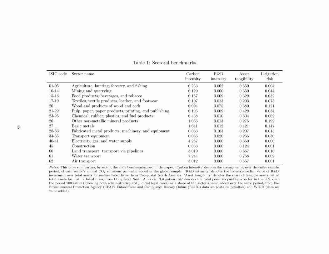
Table 1: Sectoral benchmarks

ISIC code Sector name Carbonintensity

R&Dintensity

Assettangibility

Litigationrisk

01-05 Agriculture, hunting, forestry, and fishing 0.233 0.002 0.350 0.00410-14 Mining and quarrying 0.129 0.000 0.350 0.04415-16 Food products, beverages, and tobacco 0.167 0.009 0.329 0.03217-19 Textiles, textile products, leather, and footwear 0.107 0.013 0.203 0.07520 Wood and products of wood and cork 0.094 0.075 0.380 0.12121-22 Pulp, paper, paper products, printing, and publishing 0.195 0.009 0.429 0.03423-25 Chemical, rubber, plastics, and fuel products 0.438 0.010 0.304 0.06226 Other non-metallic mineral products 1.066 0.013 0.275 0.19227 Basic metals 1.641 0.012 0.421 0.14728-33 Fabricated metal products, machinery, and equipment 0.033 0.103 0.207 0.01534-35 Transport equipment 0.056 0.020 0.255 0.03040-41 Electricity, gas, and water supply 4.257 0.000 0.350 0.00045 Construction 0.033 0.000 0.124 0.00160 Land transport transport via pipelines 3.019 0.000 0.667 0.01661 Water transport 7.244 0.000 0.758 0.00262 Air transport 3.012 0.000 0.557 0.001

Notes: This table summarizes, by sector, the main benchmarks used in the paper. ‘Carbon intensity’ denotes the average value, over the entire sampleperiod, of each sector’s annual CO2 emissions per value added in the global sample. ‘R&D intensity’ denotes the industry-median value of R&Dinvestment over total assets for mature listed firms, from Compustat North America. ‘Asset tangibility’ denotes the share of tangible assets out oftotal assets for mature listed firms, from Compustat North America. ‘Litigation risk’ denotes the total penalties paid by a sector in the U.S. overthe period 2000-2014 (following both administrative and judicial legal cases) as a share of the sector’s value added over the same period, from theEnvironmental Protection Agency (EPA)’s Enforcement and Compliance History Online (ECHO) data set (data on penalties) and WIOD (data onvalue added).

45

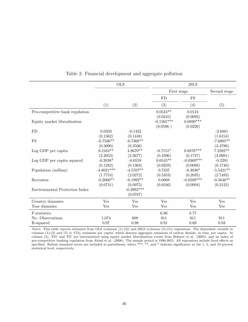
Table 2: Financial development and aggregate pollution

OLS 2SLS

First stage Second stage

FD FS

(1) (2) (3) (4) (5)

Pro-competitive bank regulation 0.0534** 0.0124(0.0245) (0.0093)

Equity market liberalization -0.1565*** 0.0890***(0.0596 ) (0.0226)

FD 0.0333 -0.1422 -2.6861(0.1362) (0.1448) (1.6154)

FS -0.7336** -0.7308** -7.6905**(0.3090) (0.3506) (3.4790)

Log GDP per capita 6.2162** 4.8670** -0.7151* 0.6876*** 7.2392**(2.2053) (2.3677) (0.4596) (0.1747) (3.0981)

Log GDP per capita squared -0.2038* -0.0559 0.0545** -0.0369*** -0.2291(0.1282) (0.1363) (0.0259) (0.0098) (0.1740)

Population (million) -4.8021*** -4.5707** 0.7337 -0.3836* -5.5421**(1.7754) (2.0272) (0.5353) (0.2035) (2.7483)

Recession -0.2060** -0.1992** 0.0068 -0.0509*** -0.5646**(0.0741) (0.0975) (0.0246) (0.0094) (0.2123)

Environmental Protection Index -0.2993***(0.0787)

Country dummies Yes Yes Yes Yes YesYear dummies Yes Yes Yes Yes Yes

F-statistics 6.96 8.77No. Observations 1,074 608 911 911 911R-squared 0.97 0.98 0.91 0.69 0.93

Notes: This table reports estimates from OLS (columns (1)-(2)) and 2SLS (columns (3)-(5)) regressions. The dependent variable incolumns (1)-(2) and (5) is ‘CO2 emissions per capita’ which denotes aggregate emissions of carbon dioxide, in tons, per capita. Incolumn (5), ‘FD’ and ‘FS’ are instrumented using equity market liberalization events from Bekaert et al. (2005), and an index ofpro-competitive banking regulation from Abiad et al. (2008). The sample period is 1990-2015. All regressions include fixed effects asspecified. Robust standard errors are included in parentheses, where ***, **, and * indicate significance at the 1, 5, and 10 percentstatistical level, respectively.

46

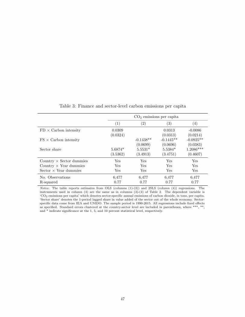
Table 3: Finance and sector-level carbon emissions per capita

CO2 emissions per capita

(1) (2) (3) (4)

FD × Carbon intensity 0.0309 0.0313 -0.0086(0.0324) (0.0313) (0.0214)

FS × Carbon intensity -0.1438** -0.1445** -0.0925**(0.0699) (0.0696) (0.0383)

Sector share 5.6874* 5.5531* 5.5384* 1.2086***(3.5362) (3.4913) (3.4751) (0.4607)

Country × Sector dummies Yes Yes Yes YesCountry × Year dummies Yes Yes Yes YesSector × Year dummies Yes Yes Yes Yes

No. Observations 6,477 6,477 6,477 6,477R-squared 0.77 0.77 0.77 0.77

Notes: The table reports estimates from OLS (columns (1)-(3)) and 2SLS (column (4)) regressions. Theinstruments used in column (4) are the same as in columns (3)-(4) of Table 2. The dependent variable is‘CO2 emissions per capita’ which denotes sector-specific annual emissions of carbon dioxide, in tons, per capita.‘Sector share’ denotes the 1-period lagged share in value added of the sector out of the whole economy. Sector-specific data come from IEA and UNIDO. The sample period is 1990-2015. All regressions include fixed effectsas specified. Standard errors clustered at the country-sector level are included in parentheses, where ***, **,and * indicate significance at the 1, 5, and 10 percent statistical level, respectively.

47

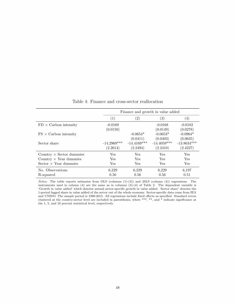
Table 4: Finance and cross-sector reallocation

Finance and growth in value added

(1) (2) (3) (4)

FD × Carbon intensity -0.0169 -0.0168 -0.0182(0.0150) (0.0149) (0.0278)

FS × Carbon intensity -0.0654* -0.0653* -0.0964*(0.0411) (0.0403) (0.0635)

Sector share -14.2969*** -14.4169*** -14.4059*** -13.8634***(2.2614) (2.2494) (2.2410) (2.4227)

Country × Sector dummies Yes Yes Yes YesCountry × Year dummies Yes Yes Yes YesSector × Year dummies Yes Yes Yes Yes

No. Observations 6,229 6,229 6,229 6,197R-squared 0.56 0.56 0.56 0.51

Notes: The table reports estimates from OLS (columns (1)-(3)) and 2SLS (column (4)) regressions. Theinstruments used in column (4) are the same as in columns (3)-(4) of Table 2. The dependent variable is‘Growth in value added’ which denotes annual sector-specific growth in value added. ‘Sector share’ denotes the1-period lagged share in value added of the sector out of the whole economy. Sector-specific data come from IEAand UNIDO. The sample period is 1990-2015. All regressions include fixed effects as specified. Standard errorsclustered at the country-sector level are included in parentheses, where ***, **, and * indicate significance atthe 1, 5, and 10 percent statistical level, respectively.

48

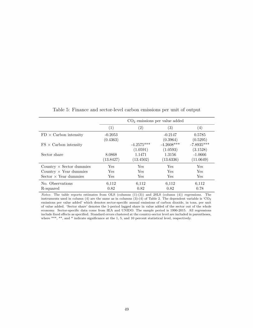
Table 5: Finance and sector-level carbon emissions per unit of output

CO2 emissions per value added

(1) (2) (3) (4)

FD × Carbon intensity -0.2053 -0.2147 0.5785(0.4363) (0.3964) (0.5295)

FS × Carbon intensity -4.2575*** -4.2608*** -7.8935***(1.0591) (1.0593) (3.1528)

Sector share 8.0868 1.1471 1.3156 -1.0666(13.8427) (13.4502) (13.6336) (11.0649)

Country × Sector dummies Yes Yes Yes YesCountry × Year dummies Yes Yes Yes YesSector × Year dummies Yes Yes Yes Yes

No. Observations 6,112 6,112 6,112 6,112R-squared 0.82 0.82 0.82 0.78

Notes: The table reports estimates from OLS (columns (1)-(3)) and 2SLS (column (4)) regressions. Theinstruments used in column (4) are the same as in columns (3)-(4) of Table 2. The dependent variable is ‘CO2

emissions per value added’ which denotes sector-specific annual emissions of carbon dioxide, in tons, per unitof value added. ‘Sector share’ denotes the 1-period lagged share in value added of the sector out of the wholeeconomy. Sector-specific data come from IEA and UNIDO. The sample period is 1990-2015. All regressionsinclude fixed effects as specified. Standard errors clustered at the country-sector level are included in parentheses,where ***, **, and * indicate significance at the 1, 5, and 10 percent statistical level, respectively.

49

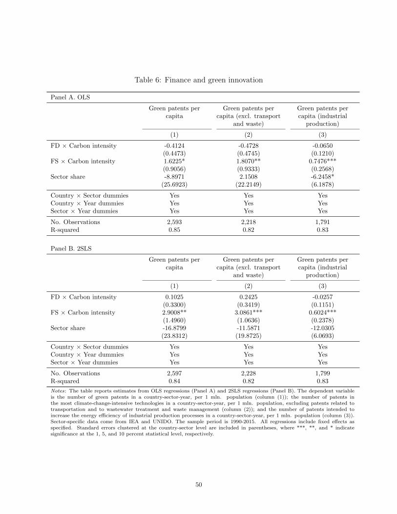
Table 6: Finance and green innovation

Panel A. OLS

Green patents percapita

Green patents percapita (excl. transport

and waste)

Green patents percapita (industrial

production)

(1) (2) (3)

FD × Carbon intensity -0.4124 -0.4728 -0.0650(0.4473) (0.4745) (0.1210)

FS × Carbon intensity 1.6225* 1.8070** 0.7476***(0.9056) (0.9333) (0.2568)

Sector share -8.8971 2.1508 -6.2458*(25.6923) (22.2149) (6.1878)

Country × Sector dummies Yes Yes YesCountry × Year dummies Yes Yes YesSector × Year dummies Yes Yes Yes

No. Observations 2,593 2,218 1,791R-squared 0.85 0.82 0.83

Panel B. 2SLS

Green patents percapita

Green patents percapita (excl. transport

and waste)

Green patents percapita (industrial

production)

(1) (2) (3)

FD × Carbon intensity 0.1025 0.2425 -0.0257(0.3300) (0.3419) (0.1151)

FS × Carbon intensity 2.9008** 3.0861*** 0.6024***(1.4960) (1.0636) (0.2378)

Sector share -16.8799 -11.5871 -12.0305(23.8312) (19.8725) (6.0693)

Country × Sector dummies Yes Yes YesCountry × Year dummies Yes Yes YesSector × Year dummies Yes Yes Yes

No. Observations 2,597 2,228 1,799R-squared 0.84 0.82 0.83

Notes: The table reports estimates from OLS regressions (Panel A) and 2SLS regressions (Panel B). The dependent variableis the number of green patents in a country-sector-year, per 1 mln. population (column (1)); the number of patents inthe most climate-change-intensive technologies in a country-sector-year, per 1 mln. population, excluding patents related totransportation and to wastewater treatment and waste management (column (2)); and the number of patents intended toincrease the energy efficiency of industrial production processes in a country-sector-year, per 1 mln. population (column (3)).Sector-specific data come from IEA and UNIDO. The sample period is 1990-2015. All regressions include fixed effects asspecified. Standard errors clustered at the country-sector level are included in parentheses, where ***, **, and * indicatesignificance at the 1, 5, and 10 percent statistical level, respectively.

50

Table 7: Finance and sector-level carbon emissions: OECD countries

CO2 emissions per capita Growth in value added CO2 emissions pervalue added

OLS 2SLS OLS 2SLS OLS 2SLS

(1) (2) (3) (4) (5) (6)

FD × Carbon intensity -0.0059 -0.0151 0.0080 0.0125 -0.0993 0.2213*(0.0171) (0.0269) (0.0102) (0.0143) (0.1203) (0.1276)

FS × Carbon intensity -0.1760*** -0.0920** -0.0120 0.0436 -1.6519*** -5.5866***(0.0550) (0.0448) (0.0400) (0.0804) (0.3522) (1.2686)

Sector share 0.5653 0.4912 -4.7391*** -3.9138*** -0.3212 0.7121(0.4325) (0.3319) (0.9607) (0.6807) (1.0936) (1.3691)

Country × Sector dummies Yes Yes Yes Yes Yes YesCountry × Year dummies Yes Yes Yes Yes Yes YesSector × Year dummies Yes Yes Yes Yes Yes Yes

No. Observations 3,368 3,368 3,132 3,132 3,210 3,210R-squared 0.94 0.94 0.62 0.60 0.88 0.86

Notes: The table reports estimates from OLS regressions (columns (1), (3), and (5)), and 2SLS regressions (columns (2), (4), and (6)).The dependent variable is the sector’s annual emissions of carbon dioxide, in tons, per capita (columns (1) and (2)); the sector’s annualgrowth in value added (columns (3) and (4)); and the sector’s annual emissions of carbon dioxide, in tons, per unit of value added(columns (5) and (6)). Sector-specific data for 33 OECD countries come from IEA and STAN. The sample period is 1990-2015. Allregressions include fixed effects as specified. Standard errors clustered at the country-sector level are included in parentheses, where***, **, and * indicate significance at the 1, 5, and 10 percent statistical level, respectively.

51

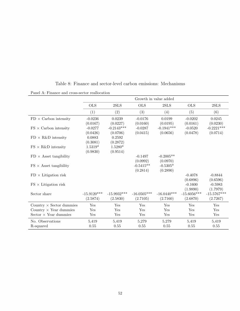
Table 8: Finance and sector-level carbon emissions: Mechanisms

Panel A: Finance and cross-sector reallocation

Growth in value added

OLS 2SLS OLS 2SLS OLS 2SLS

(1) (2) (3) (4) (5) (6)

FD × Carbon intensity -0.0236 0.0239 -0.0176 0.0199 -0.0202 0.0245(0.0167) (0.0227) (0.0160) (0.0195) (0.0161) (0.0230)

FS × Carbon intensity -0.0277 -0.2143*** -0.0287 -0.1941*** -0.0520 -0.2221***(0.0426) (0.0706) (0.0415) (0.0656) (0.0478) (0.0714)

FD × R&D intensity 0.0883 0.2592(0.3081) (0.2872)

FS × R&D intensity 1.5319* 1.5280*(0.9830) (0.9514)

FD × Asset tangibility -0.1497 -0.2005**(0.0992) (0.0970)

FS × Asset tangibility -0.5415** -0.5305*(0.2814) (0.2890)

FD × Litigation risk -0.4078 -0.8844(0.6896) (0.6596)

FS × Litigation risk -0.1600 -0.5983(1.9890) (1.7979)

Sector share -15.9120*** -15.9932*** -16.0505*** -16.0440*** -15.6056*** -15.5767***(2.5874) (2.5830) (2.7105) (2.7160) (2.6870) (2.7267)

Country × Sector dummies Yes Yes Yes Yes Yes YesCountry × Year dummies Yes Yes Yes Yes Yes YesSector × Year dummies Yes Yes Yes Yes Yes Yes

No. Observations 5,419 5,419 5,279 5,279 5,419 5,419R-squared 0.55 0.55 0.55 0.55 0.55 0.55

52

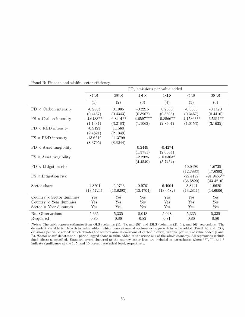
Panel B: Finance and within-sector efficiency

CO2 emissions per value added

OLS 2SLS OLS 2SLS OLS 2SLS

(1) (2) (3) (4) (5) (6)

FD × Carbon intensity -0.2553 0.1905 -0.2215 0.2533 -0.3555 -0.1470(0.4457) (0.4343) (0.3907) (0.3695) (0.3457) (0.4416)

FS × Carbon intensity -4.6483** -6.8401** -4.6597*** -5.8566** -4.1536*** -6.5611**(1.1381) (3.2183) (1.1063) (2.8407) (1.0153) (3.1625)

FD × R&D intensity -0.9123 1.1560(2.4821) (2.1349)

FS × R&D intensity -13.6212 11.3799(8.3795) (8.8244)

FD × Asset tangibility 0.2449 -0.4274(1.3751) (2.0364)

FS × Asset tangibility -2.2926 -10.8363*(4.4549) (5.7454)

FD × Litigation risk 10.0498 1.6725(12.7883) (17.6392)

FS × Litigation risk -22.4192 -91.9465**(36.5820) (43.4210)

Sector share -1.8204 -2.9763 -9.9761 -6.4004 -3.8441 1.9620(13.5724) (13.6293) (13.4704) (13.0582) (13.2811) (14.6006)

Country × Sector dummies Yes Yes Yes Yes Yes YesCountry × Year dummies Yes Yes Yes Yes Yes YesSector × Year dummies Yes Yes Yes Yes Yes Yes

No. Observations 5,335 5,335 5,048 5,048 5,335 5,335R-squared 0.80 0.80 0.82 0.81 0.80 0.80

Notes: The table reports estimates from OLS (columns (1), (3), and (5)) and 2SLS (columns (2), (4), and (6)) regressions. Thedependent variable is ‘Growth in value added’ which denotes annual sector-specific growth in value added (Panel A) and ‘CO2

emissions per value added’ which denotes the sector’s annual emissions of carbon dioxide, in tons, per unit of value added (PanelB). ‘Sector share’ denotes the 1-period lagged share in value added of the sector out of the whole economy. All regressions includefixed effects as specified. Standard errors clustered at the country-sector level are included in parentheses, where ***, **, and *indicate significance at the 1, 5, and 10 percent statistical level, respectively.

53

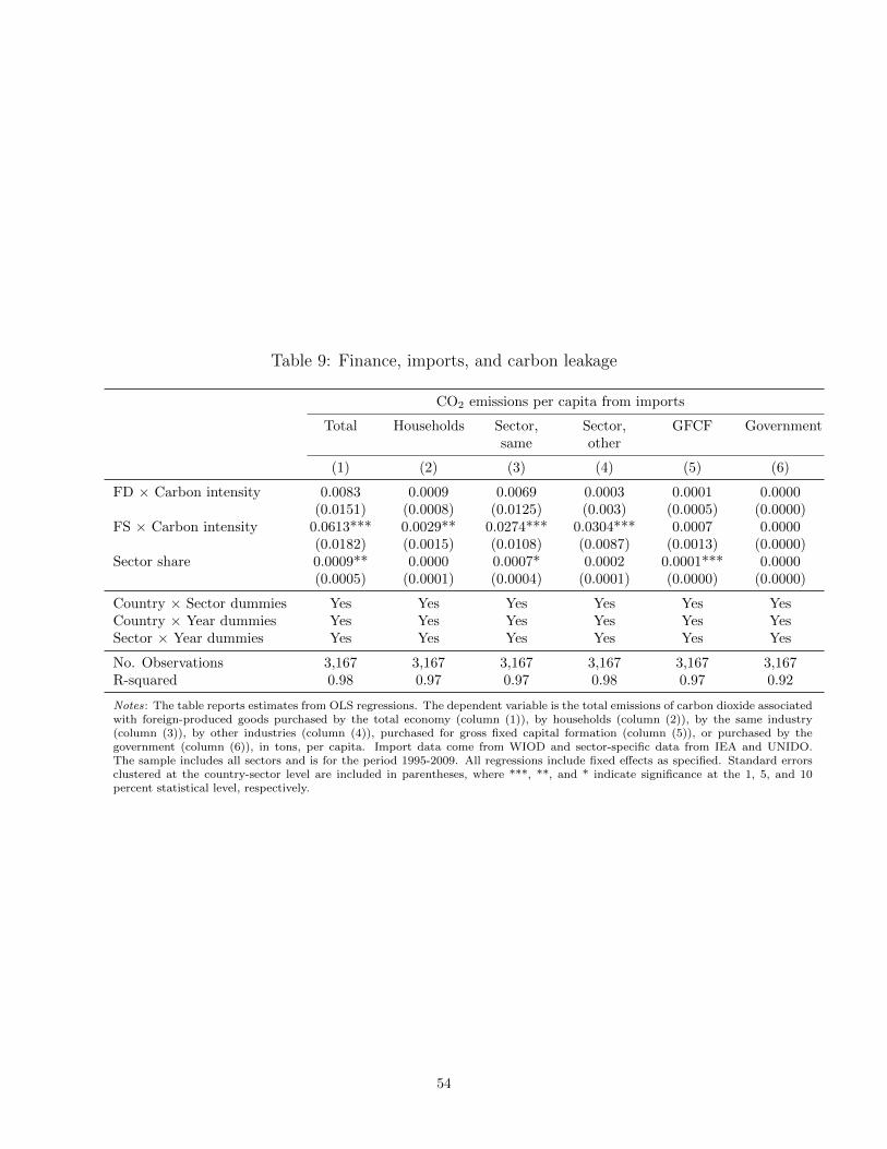
Table 9: Finance, imports, and carbon leakage

CO2 emissions per capita from imports

Total Households Sector,same

Sector,other

GFCF Government

(1) (2) (3) (4) (5) (6)

FD × Carbon intensity 0.0083 0.0009 0.0069 0.0003 0.0001 0.0000(0.0151) (0.0008) (0.0125) (0.003) (0.0005) (0.0000)

FS × Carbon intensity 0.0613*** 0.0029** 0.0274*** 0.0304*** 0.0007 0.0000(0.0182) (0.0015) (0.0108) (0.0087) (0.0013) (0.0000)

Sector share 0.0009** 0.0000 0.0007* 0.0002 0.0001*** 0.0000(0.0005) (0.0001) (0.0004) (0.0001) (0.0000) (0.0000)

Country × Sector dummies Yes Yes Yes Yes Yes YesCountry × Year dummies Yes Yes Yes Yes Yes YesSector × Year dummies Yes Yes Yes Yes Yes Yes

No. Observations 3,167 3,167 3,167 3,167 3,167 3,167R-squared 0.98 0.97 0.97 0.98 0.97 0.92

Notes: The table reports estimates from OLS regressions. The dependent variable is the total emissions of carbon dioxide associatedwith foreign-produced goods purchased by the total economy (column (1)), by households (column (2)), by the same industry(column (3)), by other industries (column (4)), purchased for gross fixed capital formation (column (5)), or purchased by thegovernment (column (6)), in tons, per capita. Import data come from WIOD and sector-specific data from IEA and UNIDO.The sample includes all sectors and is for the period 1995-2009. All regressions include fixed effects as specified. Standard errorsclustered at the country-sector level are included in parentheses, where ***, **, and * indicate significance at the 1, 5, and 10percent statistical level, respectively.

54

Table 10: Finance and pollution: Firm-level evidence

Panel A. Belgium

Equity ratio CO2 emissions persales

CO2 emissions perassets

(1) (2) (3)

Post 2006 0.0989***(0.0058)

Post 2006 × Carbon intensity -0.0011*** -0.0001***(0.0002) (0.0000)

Firm fixed effects Yes Yes YesYear dummies No Yes YesNo. Observations 3,240 1,773 1,821No. Firms 159 159 159R-squared 0.55 0.66 0.80

Panel B. Difference-in-Differences (Belgium vs. the Netherlands)

Equity ratio CO2 emissions persales

CO2 emissions perassets

(1) (2) (3)

Post 2006 0.0615***(0.0084)

Post 2006 × Belgium 0.0374***(0.0103)

Post 2006 × Carbon intensity 0.0000 -0.0001(0.0002) (0.0001)

Post 2006 × Carbon intensity × Belgium -0.0011*** -0.0001*(0.0002) (0.0000)

Firm fixed effects Yes Yes YesCountry × Year dummies No Yes YesNo. Observations 5,020 2,356 2,676No. Firms 260 260 260R-squared 0.56 0.66 0.83

Panel C. Difference-in-Differences (Matched sample: Belgium, France, Germany, Luxembourg, and the Netherlands)

Equity ratio CO2 emissions persales

CO2 emissions perassets

(1) (2) (3)

Post 2006 0.0061(0.0066)

Post 2006 × Belgium 0.0938***(0.0090)

Post 2006 × Carbon intensity 0.1292*** 0.1466***(0.0460) (0.0336)

Post 2006 × Carbon intensity × Belgium -0.1093** -0.1373***(0.0515) (0.0429)

Firm fixed effects Yes Yes YesCountry × Year dummies No Yes YesNo. Observations 5,809 3,165 3,287No. Firms 296 296 296R-squared 0.58 0.93 0.93

Notes: This table reports estimates from OLS regressions (Panel A); difference-in-differences regressions (Panel B); anddifference-in-differences regressions combined with nearest neighbor matching (Panel C). The dependent variables arethe ratio of the firm’s shareholder funds to total current plus non-current liabilities (column (1)); the firm’s emissionsof carbon dioxide equivalent, in tons, divided by total sales (column (2)); and the firm’s emissions of carbon dioxideequivalent, in tons, divided by total assets (column (3)). Belgium introduced an allowance for corporate equity (ACE)in 2006. ‘Post’ is a dummy variable equal to one in 2007 and thereafter. ‘Carbon intensity’ denotes the sector average,over the entire period 2005-2018, of firms’ CO2 equivalent emissions per sales (column (2)) or per assets (column (3)), forthe 33 countries for which firm-level CO2 equivalent data are available from the ETS. Data on equity ratios, sales, andassets come from Orbis. The sample period is 19952018 (column (1)) and 20052018 (columns (2)-(3)). All regressionsinclude fixed effects as specified. Standard errors are included in parentheses, where ***, **, and * indicate significanceat the 1, 5, and 10 percent statistical level, respectively.

55

Appendix

Table A1: Variable definitions and sources

Variable Definition Data source

CO2 emissions percapita

Aggregate or sector-specific emissions of carbon dioxide, in tons,divided by the country’s population.

UNIDO; OECD

Financial development(FD)

Sum of private-sector credit and value of all listed stocks,divided by the country’s GDP, 1-period lagged.

Beck et al. (2019)

FD with bondsSum of credit to the private sector, the value of all listed stocks,and the value of all issued private corporate bonds, divided bythe country’s GDP, 1-period lagged.

Beck et al. (2019)

Financial structure(FS)

Value of all listed stocks, divided by the sum of credit to theprivate sector and the value of all listed stocks, 1-period lagged.

Beck et al. (2019)

FS with bondsSum of the value of all listed stocks divided by the sum of creditto the private sector, the value of all listed stocks, and the valueof all issued private corporate bonds 1-period lagged.

Beck et al. (2019)

GDP per capita Country’s per capita GDP. WDI

Population Country’s population, in millions of inhabitants. WDI

RecessionDummy variable equal to 1 if the country experiences negativeGDP growth.

WDI

Environmentalprotection index

Index that measures the stringency of environmental protectiontaking values from 0 (not stringent) to 6 (very stringent).

OECD; Bottaand Kozluk(2014)

Pro-competitive bankregulation

Index of how pro-bank entry regulation is. Values of 4 or 5indicate fully liberalized; 3 indicates largely liberalized; 2 or 1indicates partially repressed and 0 indicates fully repressed.

Abiad et al.(2008)

Equity marketliberalization

Dummy variable equal to 1 if the country’s stock market is opento foreign portfolio investment.

Bekaert et al.(2005)

Growth in value added Sector-specific growth in value added. UNIDO; OECD

CO2 emissions pervalue added

Aggregate or sector-specific emissions of carbon dioxide, in tons,divided by the sector’s value added (in thousand dollars).

UNIDO; OECD

Imported CO2

emissions per capitaSector-specific carbon dioxide embedded in imports, in tons,divided by the country’s population.

WIOD

Continued on next page.

56

Table A1 cont.: Variable definitions and sources

Variable Definition Data source

Green patents percapita

Number of green patents in a country-sector-year, per 1 millionpopulation.

UNIDO; OECD;PATSTAT

Green patents percapita (excl. transportand waste)

Number of patents in the most climate-change-intensivetechnologies in a country-sector-year, per 1 million population,excluding patents related to transportation and to waste watertreatment and waste management.

UNIDO; OECD;PATSTAT

Green patents percapita (industrialproduction)

Number of patents related to inventions to increase the energyefficiency of industrial production or processing of goods in acountry-sector-year, per 1 million population.

UNIDO; OECD;PATSTAT

Sector share Share in value added of the sector out of the whole economy. UNIDO; OECD

Carbon intensityAverage value, over the entire sample period, of a sector’s CO2

emissions per value added in the global sample.IEA; UNIDO;STAN

Carbon intensity(contemporaneous)

Average value, for each year, of each sector’s CO2 emissions pervalue added, for all countries in the sample.

IEA; UNIDO;STAN

Carbon intensity (US)Average value, over the entire sample period, of each sector’sCO2 emissions per value added in the US.

IEA; UNIDO;STAN

R&D intensityIndustry-median value of R&D investment over total assets formature listed firms, from Compustat North America.

Laeven et al.(2006)

Asset tangibilityShare of tangible assets out of total assets for mature listedfirms, from Compustat North America.

Braun (2003)

Litigation riskTotal penalties paid by a sector in the U.S. during 2000-2014(following both administrative and judicial legal cases) as ashare of the sector’s value added over the same period.

EPA and ECHO;WIOD

Stock/GDPOne-period lagged ratio of the value of all listed stocks to thecountry’s GDP.

Beck et al. (2016)

Credit/GDPOne-period lagged ratio of credit to the private sector to thecountry’s GDP.

Beck et al. (2016)

External dependenceShare of capital investment financed with sources other thanretained earnings, for Compustat firms during 1990–2000.

Compustat

Fuel subsidiesDifference between the observed price of fuel and the benchmarkprice of fuel for a particular country-sector.

IMF EnergySubsidiesTemplate

Equity ratio Shareholder funds/current plus non-current liabilities (in %). Orbis

CO2 emissions persales

Firms’ emissions of carbon dioxide, in tons, divided by totalsales.

ETS; Orbis

CO2 emissions perassets

Firms’ emissions of carbon dioxide, in tons, divided by totalassets.

ETS; Orbis

Notes: This table provides definitions and data sources for all variables used in the paper. UNIDO: United NationsIndustrial Development Organization. OECD: Organisation for Economic Co-operation and Development. WDI: WorldDevelopment Indicators. IEA: International Energy Agency. PATSTAT: European Patent Office (EPO) Worldwide PatentStatistical Database. STAN: STAN Data set for Structural Analysis (OECD). EPA and ECHO: Environmental ProtectionAgency (EPA)’s Enforcement and Compliance History Online (ECHO) data set. WIOD: World Input-Output Database.ETS: EU Emissions Trading System. Orbis: Orbis - Bureau van Dijk.

57

Table A2: Summary statistics

Variable Mean Median St. dev. Min Max

Country-level

CO2 emissions per capita 6.784 6.008 4.908 0.098 32.404Financial development (FD) 1.242 1.111 0.814 0.028 4.159Financial structure (FS) 0.390 0.393 0.161 0.001 0.823GDP per capita 23.322 14.051 21.821 0.553 135.553Population 0.078 0.014 0.223 0.001 1.357Recession 0.246 0.000 0.412 0.000 1.000Environmental protection index 1.612 1.480 0.917 0.210 4.130Pro-competitive bank regulation 2.689 3.000 0.652 0.000 3.000Equity market liberalization 0.857 1.000 0.350 0.000 1.000

Sector-level (UNIDO)

CO2 emissions per capita 0.436 0.071 1.160 0.000 15.479Growth in value added -0.004 0.001 0.179 -1.000 1.000CO2 emissions per value added 1.457 0.269 5.148 0.000 196.941Green patents per capita 0.153 0.000 0.947 0.000 32.858Green patents per capita 0.112 0.000 0.735 0.000 28.013

(excl. transport and waste)Green patents per capita 0.044 0.000 0.243 0.000 8.354

(industrial production)Sector share 0.019 0.006 0.059 0.001 0.912

Sector-level (OECD)

CO2 emissions per capita 0.579 0.112 1.378 0.000 15.478Growth in value added 0.002 0.006 0.119 -1.000 1.000CO2 emissions per value added 1.498 0.214 5.020 0.000 216.825Green patents per capita 0.216 0.000 0.977 0.000 21.130Green patents per capita 0.165 0.000 0.825 0.000 20.850

(excl. transport and waste)Green patents per capita 0.066 0.000 0.274 0.000 6.252

(industrial production)Sector share 0.020 0.014 0.022 0.001 0.282

Firm-level (Orbis and ETS)

Equity ratio 0.395 0.381 0.256 0.000 1.000CO2 emissions per sales 0.009 0.007 0.013 0.000 0.129CO2 emissions per assets 0.012 0.009 0.014 0.000 0.098

Notes: This table summarizes the data used in the paper. Summary statistics for country-, sector- and firm-level CO2 emissions are expressed in metric tons (1000 kg). At the country- and sector-level, these variables aremeasured in kilotons (16 kg) in the regression analyses. Appendix Table A1 contains all variable definitions.

58

Chart 1: Global financial development and financial structure over time

Notes: The chart plots population-weighted global ‘Financial development’ and ‘Financial structure’ between 1975 and 2015.

59

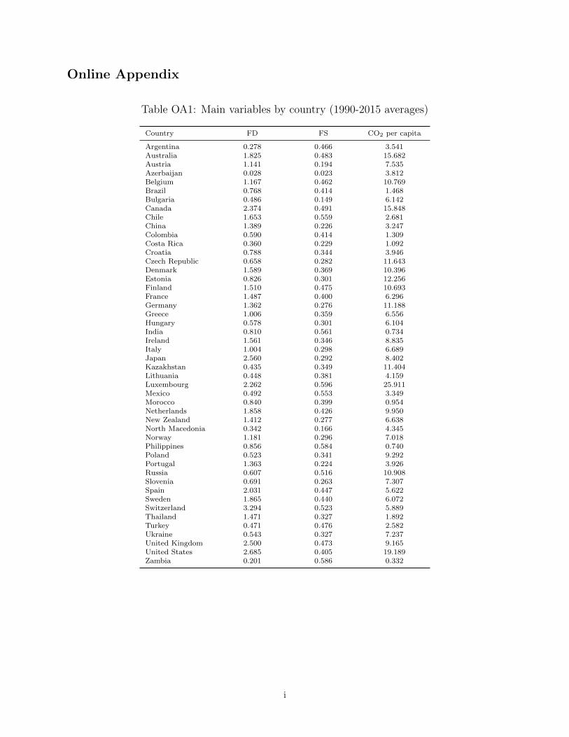
Online Appendix

Table OA1: Main variables by country (1990-2015 averages)

Country FD FS CO2 per capita

Argentina 0.278 0.466 3.541Australia 1.825 0.483 15.682Austria 1.141 0.194 7.535Azerbaijan 0.028 0.023 3.812Belgium 1.167 0.462 10.769Brazil 0.768 0.414 1.468Bulgaria 0.486 0.149 6.142Canada 2.374 0.491 15.848Chile 1.653 0.559 2.681China 1.389 0.226 3.247Colombia 0.590 0.414 1.309Costa Rica 0.360 0.229 1.092Croatia 0.788 0.344 3.946Czech Republic 0.658 0.282 11.643Denmark 1.589 0.369 10.396Estonia 0.826 0.301 12.256Finland 1.510 0.475 10.693France 1.487 0.400 6.296Germany 1.362 0.276 11.188Greece 1.006 0.359 6.556Hungary 0.578 0.301 6.104India 0.810 0.561 0.734Ireland 1.561 0.346 8.835Italy 1.004 0.298 6.689Japan 2.560 0.292 8.402Kazakhstan 0.435 0.349 11.404Lithuania 0.448 0.381 4.159Luxembourg 2.262 0.596 25.911Mexico 0.492 0.553 3.349Morocco 0.840 0.399 0.954Netherlands 1.858 0.426 9.950New Zealand 1.412 0.277 6.638North Macedonia 0.342 0.166 4.345Norway 1.181 0.296 7.018Philippines 0.856 0.584 0.740Poland 0.523 0.341 9.292Portugal 1.363 0.224 3.926Russia 0.607 0.516 10.908Slovenia 0.691 0.263 7.307Spain 2.031 0.447 5.622Sweden 1.865 0.440 6.072Switzerland 3.294 0.523 5.889Thailand 1.471 0.327 1.892Turkey 0.471 0.476 2.582Ukraine 0.543 0.327 7.237United Kingdom 2.500 0.473 9.165United States 2.685 0.405 19.189Zambia 0.201 0.586 0.332

i

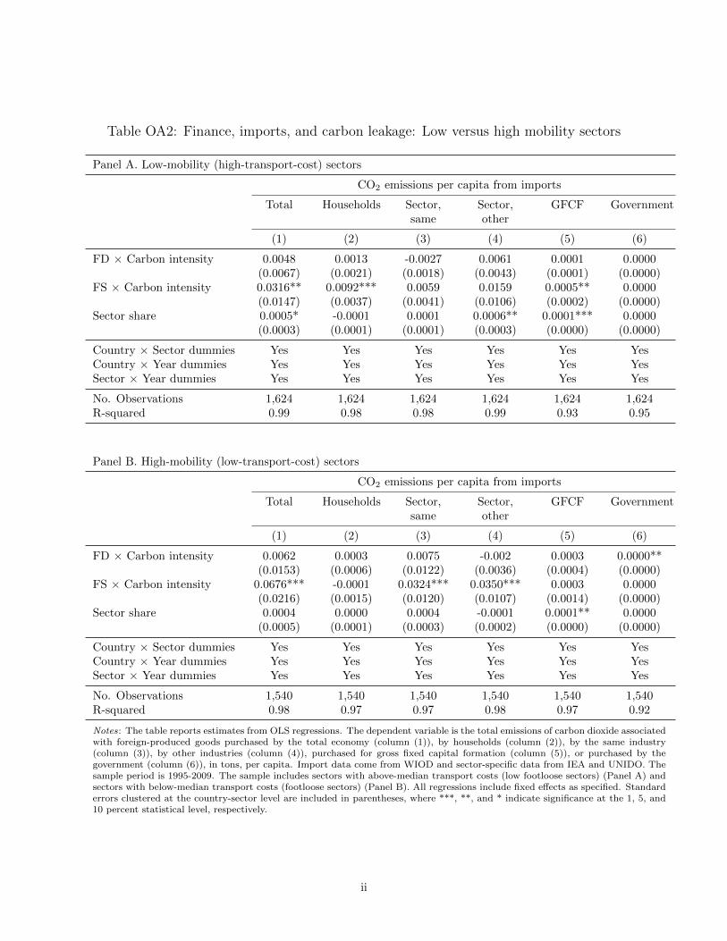
Table OA2: Finance, imports, and carbon leakage: Low versus high mobility sectors

Panel A. Low-mobility (high-transport-cost) sectors

CO2 emissions per capita from imports

Total Households Sector,same

Sector,other

GFCF Government

(1) (2) (3) (4) (5) (6)

FD × Carbon intensity 0.0048 0.0013 -0.0027 0.0061 0.0001 0.0000(0.0067) (0.0021) (0.0018) (0.0043) (0.0001) (0.0000)

FS × Carbon intensity 0.0316** 0.0092*** 0.0059 0.0159 0.0005** 0.0000(0.0147) (0.0037) (0.0041) (0.0106) (0.0002) (0.0000)

Sector share 0.0005* -0.0001 0.0001 0.0006** 0.0001*** 0.0000(0.0003) (0.0001) (0.0001) (0.0003) (0.0000) (0.0000)

Country × Sector dummies Yes Yes Yes Yes Yes YesCountry × Year dummies Yes Yes Yes Yes Yes YesSector × Year dummies Yes Yes Yes Yes Yes Yes

No. Observations 1,624 1,624 1,624 1,624 1,624 1,624R-squared 0.99 0.98 0.98 0.99 0.93 0.95

Panel B. High-mobility (low-transport-cost) sectors

CO2 emissions per capita from imports

Total Households Sector,same

Sector,other

GFCF Government

(1) (2) (3) (4) (5) (6)

FD × Carbon intensity 0.0062 0.0003 0.0075 -0.002 0.0003 0.0000**(0.0153) (0.0006) (0.0122) (0.0036) (0.0004) (0.0000)

FS × Carbon intensity 0.0676*** -0.0001 0.0324*** 0.0350*** 0.0003 0.0000(0.0216) (0.0015) (0.0120) (0.0107) (0.0014) (0.0000)

Sector share 0.0004 0.0000 0.0004 -0.0001 0.0001** 0.0000(0.0005) (0.0001) (0.0003) (0.0002) (0.0000) (0.0000)

Country × Sector dummies Yes Yes Yes Yes Yes YesCountry × Year dummies Yes Yes Yes Yes Yes YesSector × Year dummies Yes Yes Yes Yes Yes Yes

No. Observations 1,540 1,540 1,540 1,540 1,540 1,540R-squared 0.98 0.97 0.97 0.98 0.97 0.92

Notes: The table reports estimates from OLS regressions. The dependent variable is the total emissions of carbon dioxide associatedwith foreign-produced goods purchased by the total economy (column (1)), by households (column (2)), by the same industry(column (3)), by other industries (column (4)), purchased for gross fixed capital formation (column (5)), or purchased by thegovernment (column (6)), in tons, per capita. Import data come from WIOD and sector-specific data from IEA and UNIDO. Thesample period is 1995-2009. The sample includes sectors with above-median transport costs (low footloose sectors) (Panel A) andsectors with below-median transport costs (footloose sectors) (Panel B). All regressions include fixed effects as specified. Standarderrors clustered at the country-sector level are included in parentheses, where ***, **, and * indicate significance at the 1, 5, and10 percent statistical level, respectively.

ii

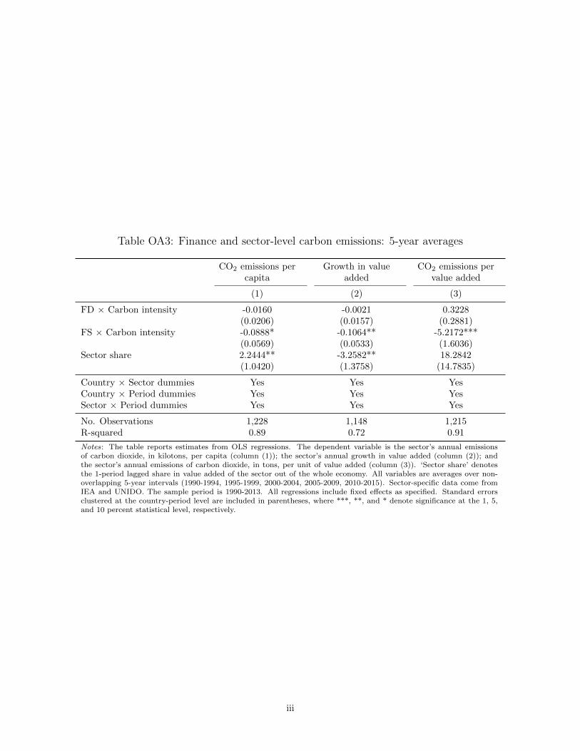
Table OA3: Finance and sector-level carbon emissions: 5-year averages

CO2 emissions percapita

Growth in valueadded

CO2 emissions pervalue added

(1) (2) (3)

FD × Carbon intensity -0.0160 -0.0021 0.3228(0.0206) (0.0157) (0.2881)

FS × Carbon intensity -0.0888* -0.1064** -5.2172***(0.0569) (0.0533) (1.6036)

Sector share 2.2444** -3.2582** 18.2842(1.0420) (1.3758) (14.7835)

Country × Sector dummies Yes Yes YesCountry × Period dummies Yes Yes YesSector × Period dummies Yes Yes Yes

No. Observations 1,228 1,148 1,215R-squared 0.89 0.72 0.91

Notes: The table reports estimates from OLS regressions. The dependent variable is the sector’s annual emissionsof carbon dioxide, in kilotons, per capita (column (1)); the sector’s annual growth in value added (column (2)); andthe sector’s annual emissions of carbon dioxide, in tons, per unit of value added (column (3)). ‘Sector share’ denotesthe 1-period lagged share in value added of the sector out of the whole economy. All variables are averages over non-overlapping 5-year intervals (1990-1994, 1995-1999, 2000-2004, 2005-2009, 2010-2015). Sector-specific data come fromIEA and UNIDO. The sample period is 1990-2013. All regressions include fixed effects as specified. Standard errorsclustered at the country-period level are included in parentheses, where ***, **, and * denote significance at the 1, 5,and 10 percent statistical level, respectively.

iii

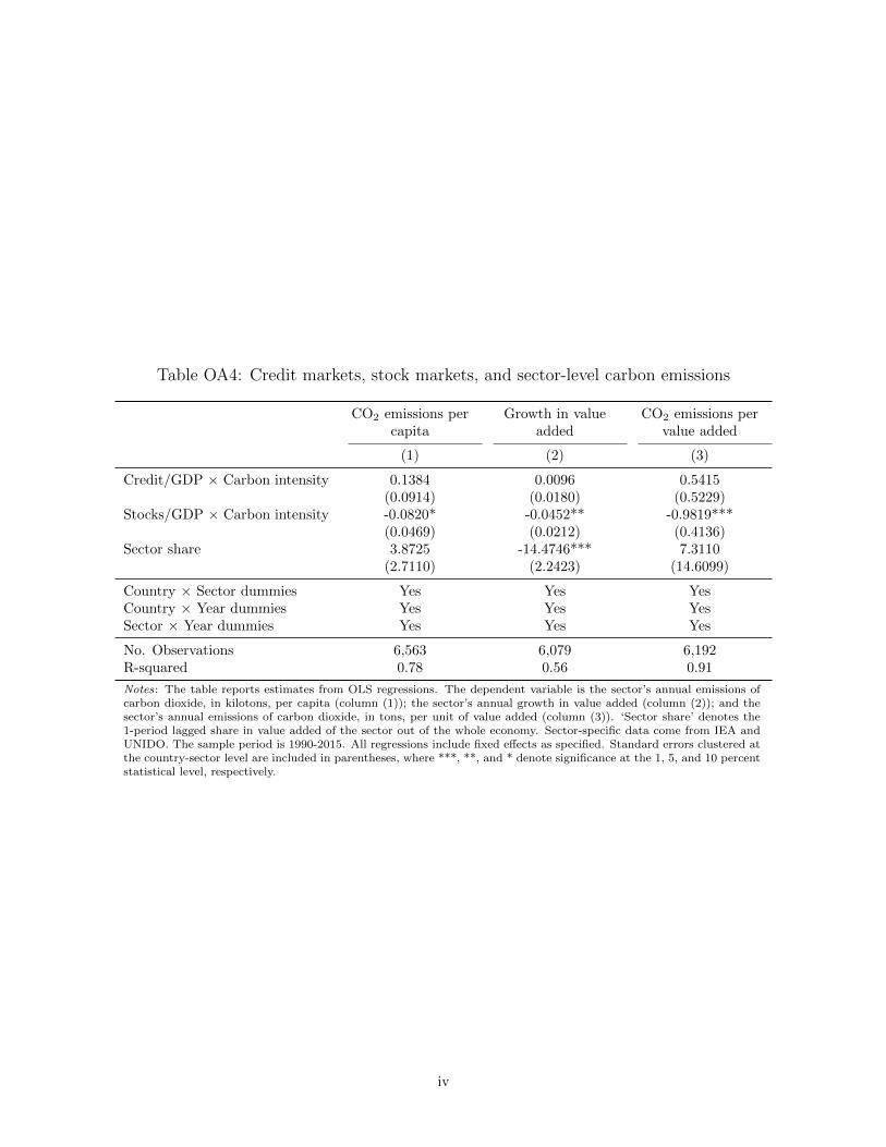
Table OA4: Credit markets, stock markets, and sector-level carbon emissions

CO2 emissions percapita

Growth in valueadded

CO2 emissions pervalue added

(1) (2) (3)

Credit/GDP × Carbon intensity 0.1384 0.0096 0.5415(0.0914) (0.0180) (0.5229)

Stocks/GDP × Carbon intensity -0.0820* -0.0452** -0.9819***(0.0469) (0.0212) (0.4136)

Sector share 3.8725 -14.4746*** 7.3110(2.7110) (2.2423) (14.6099)

Country × Sector dummies Yes Yes YesCountry × Year dummies Yes Yes YesSector × Year dummies Yes Yes Yes

No. Observations 6,563 6,079 6,192R-squared 0.78 0.56 0.91

Notes: The table reports estimates from OLS regressions. The dependent variable is the sector’s annual emissions ofcarbon dioxide, in kilotons, per capita (column (1)); the sector’s annual growth in value added (column (2)); and thesector’s annual emissions of carbon dioxide, in tons, per unit of value added (column (3)). ‘Sector share’ denotes the1-period lagged share in value added of the sector out of the whole economy. Sector-specific data come from IEA andUNIDO. The sample period is 1990-2015. All regressions include fixed effects as specified. Standard errors clustered atthe country-sector level are included in parentheses, where ***, **, and * denote significance at the 1, 5, and 10 percentstatistical level, respectively.

iv

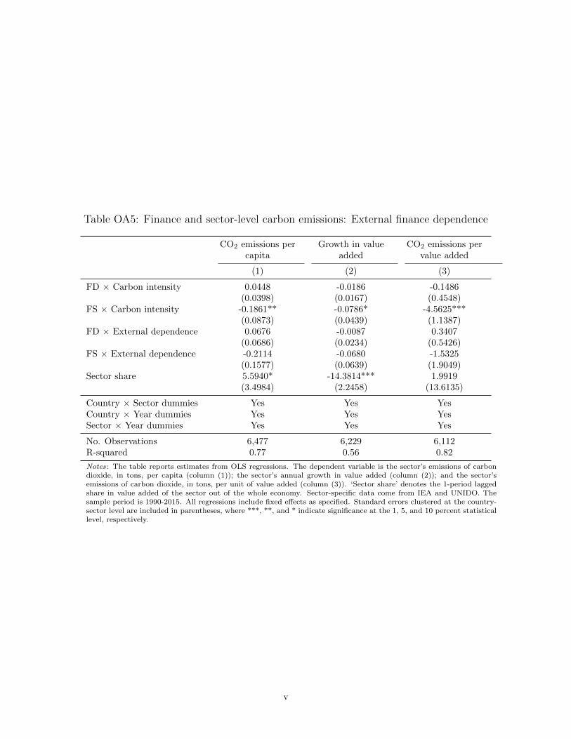
Table OA5: Finance and sector-level carbon emissions: External finance dependence

CO2 emissions percapita

Growth in valueadded

CO2 emissions pervalue added

(1) (2) (3)

FD × Carbon intensity 0.0448 -0.0186 -0.1486(0.0398) (0.0167) (0.4548)

FS × Carbon intensity -0.1861** -0.0786* -4.5625***(0.0873) (0.0439) (1.1387)

FD × External dependence 0.0676 -0.0087 0.3407(0.0686) (0.0234) (0.5426)

FS × External dependence -0.2114 -0.0680 -1.5325(0.1577) (0.0639) (1.9049)

Sector share 5.5940* -14.3814*** 1.9919(3.4984) (2.2458) (13.6135)

Country × Sector dummies Yes Yes YesCountry × Year dummies Yes Yes YesSector × Year dummies Yes Yes Yes

No. Observations 6,477 6,229 6,112R-squared 0.77 0.56 0.82

Notes: The table reports estimates from OLS regressions. The dependent variable is the sector’s emissions of carbondioxide, in tons, per capita (column (1)); the sector’s annual growth in value added (column (2)); and the sector’semissions of carbon dioxide, in tons, per unit of value added (column (3)). ‘Sector share’ denotes the 1-period laggedshare in value added of the sector out of the whole economy. Sector-specific data come from IEA and UNIDO. Thesample period is 1990-2015. All regressions include fixed effects as specified. Standard errors clustered at the country-sector level are included in parentheses, where ***, **, and * indicate significance at the 1, 5, and 10 percent statisticallevel, respectively.

v

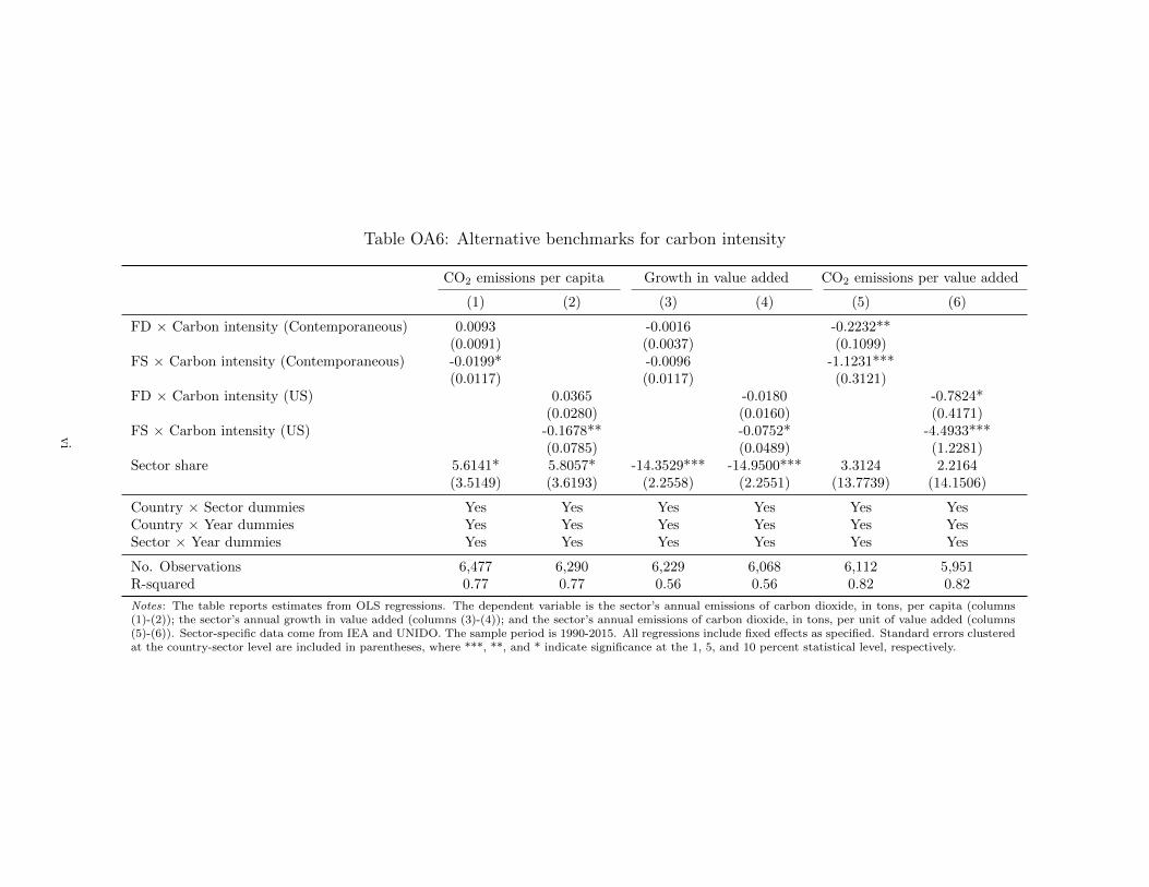
Table OA6: Alternative benchmarks for carbon intensity

CO2 emissions per capita Growth in value added CO2 emissions per value added

(1) (2) (3) (4) (5) (6)

FD × Carbon intensity (Contemporaneous) 0.0093 -0.0016 -0.2232**(0.0091) (0.0037) (0.1099)

FS × Carbon intensity (Contemporaneous) -0.0199* -0.0096 -1.1231***(0.0117) (0.0117) (0.3121)

FD × Carbon intensity (US) 0.0365 -0.0180 -0.7824*(0.0280) (0.0160) (0.4171)

FS × Carbon intensity (US) -0.1678** -0.0752* -4.4933***(0.0785) (0.0489) (1.2281)

Sector share 5.6141* 5.8057* -14.3529*** -14.9500*** 3.3124 2.2164(3.5149) (3.6193) (2.2558) (2.2551) (13.7739) (14.1506)

Country × Sector dummies Yes Yes Yes Yes Yes YesCountry × Year dummies Yes Yes Yes Yes Yes YesSector × Year dummies Yes Yes Yes Yes Yes Yes

No. Observations 6,477 6,290 6,229 6,068 6,112 5,951R-squared 0.77 0.77 0.56 0.56 0.82 0.82

Notes: The table reports estimates from OLS regressions. The dependent variable is the sector’s annual emissions of carbon dioxide, in tons, per capita (columns(1)-(2)); the sector’s annual growth in value added (columns (3)-(4)); and the sector’s annual emissions of carbon dioxide, in tons, per unit of value added (columns(5)-(6)). Sector-specific data come from IEA and UNIDO. The sample period is 1990-2015. All regressions include fixed effects as specified. Standard errors clusteredat the country-sector level are included in parentheses, where ***, **, and * indicate significance at the 1, 5, and 10 percent statistical level, respectively.

vi

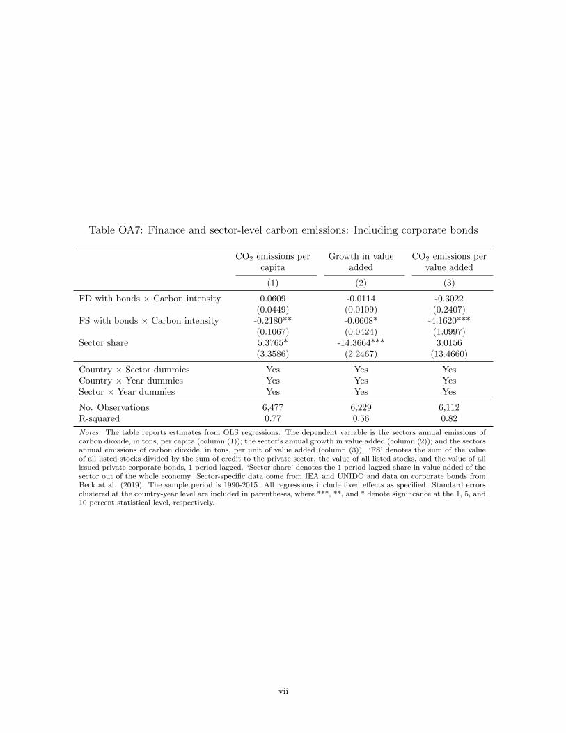
Table OA7: Finance and sector-level carbon emissions: Including corporate bonds

CO2 emissions percapita

Growth in valueadded

CO2 emissions pervalue added

(1) (2) (3)

FD with bonds × Carbon intensity 0.0609 -0.0114 -0.3022(0.0449) (0.0109) (0.2407)

FS with bonds × Carbon intensity -0.2180** -0.0608* -4.1620***(0.1067) (0.0424) (1.0997)

Sector share 5.3765* -14.3664*** 3.0156(3.3586) (2.2467) (13.4660)

Country × Sector dummies Yes Yes YesCountry × Year dummies Yes Yes YesSector × Year dummies Yes Yes Yes

No. Observations 6,477 6,229 6,112R-squared 0.77 0.56 0.82

Notes: The table reports estimates from OLS regressions. The dependent variable is the sectors annual emissions ofcarbon dioxide, in tons, per capita (column (1)); the sector’s annual growth in value added (column (2)); and the sectorsannual emissions of carbon dioxide, in tons, per unit of value added (column (3)). ‘FS’ denotes the sum of the valueof all listed stocks divided by the sum of credit to the private sector, the value of all listed stocks, and the value of allissued private corporate bonds, 1-period lagged. ‘Sector share’ denotes the 1-period lagged share in value added of thesector out of the whole economy. Sector-specific data come from IEA and UNIDO and data on corporate bonds fromBeck at al. (2019). The sample period is 1990-2015. All regressions include fixed effects as specified. Standard errorsclustered at the country-year level are included in parentheses, where ***, **, and * denote significance at the 1, 5, and10 percent statistical level, respectively.

vii

Table OA8: Finance and sector-level carbon emissions: Including private equity

CO2 emissions percapita

Growth in valueadded

CO2 emissions pervalue added

(1) (2) (3)

FD × Carbon intensity 0.0514 0.0063 -0.4776(0.0433) (0.0171) (0.6563)

FS × Carbon intensity -0.2174** -0.0232 -5.9141***(0.0947) (0.0581) (1.7080)

Sector share 16.9155* -12.5589*** 3.6895(10.6717) (2.2024) (18.1962)

Country × Sector dummies Yes Yes YesCountry × Year dummies Yes Yes YesSector × Year dummies Yes Yes Yes

No. Observations 3,688 3,548 3,593R-squared 0.76 0.57 0.74

Notes: The table reports estimates from OLS regressions. The dependent variable is the sector’s annual emissions of carbondioxide, in tons, per capita (column (1)); the sector’s annual growth in value added (column (2)); and the sector’s annualemissions of carbon dioxide, in tons, per unit of value added (column (3)). Sector-specific data come from IEA and UNIDOand data on private equity from the European Venture Capital Association. The sample period is 1990-2015. All regressionsinclude fixed effects as specified. Standard errors clustered at the country-sector level are included in parentheses, where ***,**, and * indicate significance at the 1, 5, and 10 percent statistical level, respectively.

viii

Table OA9: Finance and sector-level carbon emissions: Controlling for fuel subsidies

CO2 emissions percapita

Growth in valueadded

CO2 emissions pervalue added

(1) (2) (3)

FD × Carbon intensity 0.0278 -0.0160 -0.1688(0.0307) (0.0149) (0.3999)

FS × Carbon intensity -0.1503** -0.0605* -3.9049***(0.0777) (0.0424) (1.1052)

FD × Fuel subsidies 0.5756** -0.4921 -0.6325(0.2722) (0.3645) (8.5471)

FS × Fuel subsidies 0.2418 0.3190 -42.7516**(0.7594) (0.7432) (18.2014)

Sector share 5.7019* -14.6130*** -0.5884(3.6422) (2.3108) (13.4153)

Country × Sector dummies Yes Yes YesCountry × Year dummies Yes Yes YesSector × Year dummies Yes Yes Yes

No. Observations 6,167 6,079 5,806R-squared 0.77 0.56 0.84

Notes: The table reports estimates from OLS regressions. The dependent variable is the sector’s annual emissionsof carbon dioxide, in tons, per capita (column (1)); the sector’s annual growth in value added (column (2));and the sector’s annual emissions of carbon dioxide, in kilotons, per unit of value added (column (3)). Sector-specific data come from IEA, IMF, and UNIDO. The sample period is 1990-2015. All regressions include fixedeffects as specified. Standard errors clustered at the country-year level are included in parentheses, where ***,**, and * indicate significance at the 1, 5, and 10 percent statistical level, respectively.

ix

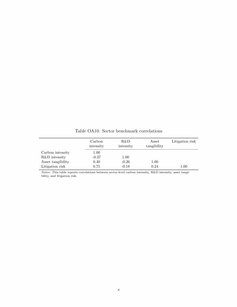
Table OA10: Sector benchmark correlations

Carbonintensity

R&Dintensity

Assettangibility

Litigation risk

Carbon intensity 1.00R&D intensity -0.37 1.00Asset tangibility 0.40 -0.26 1.00Litigation risk 0.75 -0.18 0.24 1.00

Notes: This table reports correlations between sector-level carbon intensity, R&D intensity, asset tangi-bility, and litigation risk.

x