Disease and Diversity in Long-termEconomic Development

Javier A. Birchenall∗

University of California at Santa Barbara

November 19, 2014

Abstract

Ethnographic data on large and impressive structures and archeological

censuses of cities suggest that during the pre-colonial era, sub-Saharan Africa

lacked widespread state-consolidated power typical of large tributary empires

such as the Incas and the Aztecs in tropical America. Ethnographic data also

suggest that disease (i.e., environmentally-determined pathogen stress) limited

pre-colonial economic development and state consolidation partly through a

promoting of ethnic diversity. The effects of disease and ethnic diversity persist

for a long time; pre-colonial factors continue to determine current income per

capita and current indices of ethnolinguistic fractionalization.

JEL classification: J11; O11; P51

Communications to: Javier A. Birchenall

Department of Economics, 2127 North Hall

University of California, Santa Barbara CA 93106

Phone/fax: (805) 893-5275

E-mail: Javier.Birchenall@ucsb.edu

∗I would like to thank Philip Babcock, Sambit Bhattacharyya, Hoyt Bleakley, Bob Fogel, DavidCarr, Juan Carlos Cordoba, Dave Donaldson, Stanley Engerman, James Fenske, Nicola Gennaioli, Ana

Maria Ibáñez, Hyeok Jeong, Michael Kevane, Gary Libecap, Peter Lindert, Ted Miguel, Kris Mitchener,

Nathan Nunn, Pekka Hämäläinen, Phil Hoffman, Jeff Nugent, Bonnie Queen, James Robinson, Jean-

Laurent Rosenthal, Raaj Sah, Romain Wacziarg, Warren Whatley, and seminar participants at multiple

locations for very useful comments.

1 Introduction

Africa’s transition into modern economic growth has been slow. As a focal point, the

literature on African economic growth has emphasized modern influences such as the

legacies of European colonialism and the slave trade; see, e.g., Acemoglu et al. ([1], [2],

[3]), Bates et al. [9], Glaeser et al. [34], Nunn [53], and Nunn and Wantchekon [54]. There

are also, as counterpoints, lines of continuity that emphasize pre-colonial conditions; see,

e.g., Bockstette et al. [14], Englebert [28], Fenske [29], Gennaioli and Rainer [33], Herbst

[36], Michalopoulos [47], and Michalopoulos and Papaioannou ([48], [49]). This paper is

an empirical study of comparative development that emphasizes the long-term effects of

disease. Its main thesis is that sub-Saharan Africa lagged behind comparable areas long

before the European expansion, and that Africa’s adverse disease environments have been

central in limiting social, economic, and political integration since the pre-colonial era.

A long-term perspective is important in comparative economic development because

the modern influences set off by the European expansion operated in regions with signif-

icant differences. The absence of well-established data, however, is a critical limitation

in studying the pre-colonial era. In this paper, I heavily rely on Murdock and White’s

[52] Standard Cross Cultural Sample (SCCS) though I will also consider alternative data

sources such as Chandler’s [17] inventory of medium and large cities. The SCCS consists

of disaggregate data from 186 ethnographically well-described societies with different sub-

sistence strategies. The SCCS was designed to be representative of all the pre-industrial

societies in the world and it was constructed to maximize independence in terms of cultural

and historical origin. Societies are thoroughly described from historic and ethnographic

literature at the time coinciding with or just after contact with Western cultures when

some reliable observer (i.e., traveler, missionary, trader, colonial agent, or anthropolo-

gist) first visited the society and wrote about it in sufficient detail; see, e.g., Pryor [58].

The SCCS represents the earliest systematic “snapshot” of former European colonies in

tropical Africa and the New World.

The SCCS measures various economic aspects of pre-modern societies such as the de-

gree of complexity in the buildings of a given society. Particularly, the SCCS records

1

information about the presence and scope of large or impressive structures. A physical

structure is easy to recognize by Western observers hence it is an aspect of pre-colonial so-

cieties that can be measured with relatively high precision. Interpreting physical evidence

is also less arbitrary that interpreting, for example, measures of political centralization

available in the SCCS or in their predecessors, i.e., Murdock’s [51] Ethnographic Atlas.

(Agricultural societies in sub-Saharan Africa, for instance, are on average ranked as high

as Eurasian societies in political centralization in the SCCS.1) Historically, impressive

structures are a manifestation of the state’s capacity to consolidate power, or the capac-

ity of urban elites, to extract resources from peasants. The existence of large structures

is thus a reasonable proxy for the presence of large tributary empires and the state’s

capacity to generate, extract, and mobilize resources in society.

In the SCCS, the presence and scope of large structures is significantly different be-

tween African societies and the rest of the world. Differences are evident even with respect

to tropical America, an area that was comparable to sub-Saharan Africa in many relevant

dimensions. To validate this finding, I show that Chandler’s [17] inventory of cities also

suggests that sub-Saharan Africa had fewer and less densely populated cities than tropical

America. In particular, while there were no large cities south of the Sahara around the

time of the European expansion, Teothihuacán, currently Mexico city, was among the ten

largest cities of the world in 400 AD; see Chandler ([17], p. 464). Overall, Westerners’ di-

rect accounts of large or impressive structures and archeological inventories of cities both

suggest that state structures in pre-colonial Africa were less sophisticated (i.e., smaller in

scale and scope) than those of European and Asian empires, and even less sophisticated

than those of the tributary empires of tropical America.2

Evidence drawn from the SCCS also shows that pathogen stress, a measure of the

1Gennaioli and Rainer [33], Heldring and Robinson [35], Michalopoulos and Papaioannou [48], and

Osafo-Kwaako and Robinson [55] are among the studies that rely on measures of political centralization

from the previous ethnographic surveys. Their goal is to study pre-colonial conditions within Africa and

not comparative aspects within former European colonies. Later on I discuss some shortcomings of using

measures of political centralization in the SCCS to study comparative development.2This finding conforms well with existing discussions by African economic historians who have de-

scribed pre-colonial state structures in Africa as weak; see, e.g., Connah [19], Curtin et al. [22], Englebert

[28], Fortes and Evans-Pritchard [32], Herbst [36], and Hopkins [38].

2

prevalence and severity of serious pathogenic diseases, is strongly and negatively related

with the existence and scope of large or impressive structures. This relationship is driven

primarily (but not exclusively) by African societies which, for a multiplicity of environ-

mental reasons, have faced more adverse disease environments than societies in tropical

areas elsewhere; see, e.g., Crosby [21], Curtin et al. [22], Diamond and Panosian [25],

McNeill [46], and Wolfe et al. [64]. This association is potentially causal. Reverse causal-

ity is not an important concern. Moreover, the pathogens considered here are typically

transmitted through vectors environmentally determined, they are not by-products of

changes in food production, and they have a regional distribution concentrated in trop-

ical Africa. Even as a correlative relationship, the negative association between disease

and pre-colonial development is stable and robust across numerous specifications.

The previous association does not provide a mechanism by which disease and devel-

opment interacted in the past. Parasite avoidance, however, triggers reproductive, social,

and cultural isolation between human populations; see, e.g., Azevado [8], Cashdan [16],

and Fincher and Thornhill [30]. Parasites, as Kurzban and Leary ([40], p. 192) note,

put the “brakes” on sociality. In the SCCS, African societies are indeed more ethnically

diverse than anywhere else in the world. Pathogen stress, for instance, has a strong and

positive influence on pre-colonial ethnic diversity. Moreover, the effects of disease and

ethnic diversity on economic outcomes persist for long periods of time. Pathogen stress

and pre-colonial ethnic diversity are strongly associated with current income per capita

and current indices of ethnolinguistic fractionalization. Tentatively, these findings sug-

gest that Africa’s pre-colonial and current weak state capacities (relative, for example, to

tropical America) are partly a consequence of Africa’s unique disease environment and its

fostering of ethnic diversity.

A notable feature of this paper is its focus on the pre-colonial era.3 The literature

3Economists have almost exclusivelly associated pre-colonial differences with technological disparities

often using a Malthusian logic; see, e.g., Ashraf and Galor [5]. This logic works well to account for

economic and demographic differences between agricultural areas (i.e., the Near East and China) and

non-agricultural ones (i.e., North America and Austrialia). The Malthusian logic, however, fails to account

for the comparative development of tropical areas because their technological conditions were relatively

similar.

3

typically examines direct links between pre-colonial aspects and modern outcomes. An

association between pre-colonial aspects and modern outcomes, however, could arise be-

cause of factors that pre-dated the European arrival or because of factors that emerged

in response to European influences.4 The influence of disease on current economic con-

ditions, for example, has been interpreted in direct terms (see, e.g., Bhattacharyya [11],

Bloom and Sachs [15], and Kamarck [39]) but also indirectly through the effect of settler

mortality on colonial institutions and human capital (see, e.g., Acemoglu et al. [1] and

Glaeser et al. [34]). The analysis of pre-colonial data suggests that disease limits eco-

nomic development but not exclusively through its effect on European settlements and

institutions, as argued by the colonial origin hypothesis in Acemoglu et al. [1].

The importance of disease in long-term outcomes resounds with McNeill’s [46] thesis

and related literature; e.g., Price-Smith [57], Rosen [59], and Zinsser [65]. In Plagues and

People, McNeill [46] used the historical record to show that disease limited the consoli-

dation of pre-modern states and empires contributing, for example, to the collapse of the

Roman Empire and China’s ancient Han Dynasty. Regarding Africa, McNeill ([46], p.

43) argued that

“[high exposure to disease], more than anything else, is why Africa remained

backward in the development of civilization when compared to temperate lands

(or tropical zones like those in the Americas), where prevailing ecosystems

where less elaborated and correspondingly less inimical to simplification by

human action.”

The analysis of disease and ethnic diversity also complements an emerging literature

that examines the causes of high ethnic fragmentation in Africa. Michalopoulos [47], for

example, identified a positive effect of physical barriers (i.e., barriers geographically deter-

4Methodologically, considering influences that pre-date the European arrival serves to discriminate be-

tween competing fundamental forces behind the comparative development of former European colonies.

An example of pre-dating influences is indirect rule or the use of pre-colonial intermediaries and institu-

tions to exercise colonial control. An example of emerging influences are extractive institutions motivated

by differences in disease environments or endowments. Both views are prominent in the literature; see,

e.g., Acemoglu et al. [1] and Bockstette et al. [14]. Heldring and Robinson [35] provide a recent assess-

ment of the effect of colonization in Africa that recognizes these multiple lines of influence.

4

mined) on current ethnolinguistic fractionalization and Michalopoulos and Papaioannou

[49] studied the effect political barriers (i.e., artificial country boundaries) on current eco-

nomic outcomes and civil conflict in Africa. This paper is consistent with the notion that

disease acts as a social barrier that limits social, political, and economic integration. This

argument is mathematically formulated in Birchenall [13].

The paper unfolds as follows. Section 2 introduces the main data sources; Section

3 documents the association between disease and pre-colonial development; Section 4

documents the association between pre-colonial factors and current outcomes; and Section

5 concludes.

2 Data and measurement

Societal data. The Standard Cross-Cultural Sample (SCCS) was developed by Mur-

dock and White [52] during the 1960s. The SCCS contains 186 pre-industrial societies

with various subsistence strategies, including hunter-gatherers, fishers, pastoralists, hor-

ticulturalists, and agriculturalists. The SCCS provides extensive coded data constructed

from historical records and published field research by ethnographers. Information about

these societies is obtained through narratives and descriptions of Westerners in their first

encounters with these societies. There is no “pristine” society in the SCCS; many of

the native societies in Africa were not reached by Europeans until late in the nineteenth

century or early in the twentieth century; see Table 1 below. The key, as pointed out by

Pryor ([58], pp. 24-25), is to “ask how much these preindustrial societies have changed

over the millennia until the pinpointed date.” I assume that contamination in the SCCS

is not a serious problem and that potential biases are corrected by controls for the date of

pinpointing of the society. Further, the SCCS is not a random sample of all pre-industrial

societies and, by construction, the SCCS is prone to measurement errors.5

5The societies in the SCCS are a culturally independent sub-sample of the Ethnographic Atlas, also

consolidated by George Murdock; see Murdock [52]. The Atlas contains many more societies than the

SCCS but there is less information for each society, i.e., there is no measure of physical structures in

the Atlas, which is one of the central outcomes of interest in this paper. Later sections examine current

economic outcomes.

5

The SCCS, however, has wide geographic coverage and it is the earliest and most

complete systematic assessment of pre-industrial societies in the world. The geographic

composition of the 186 societies is as follows: 32 societies are in sub-Saharan Africa, 35

in South and Central America, 24 in West Eurasia, 34 in East Eurasia, 31 in the insular

Pacific and 30 in North America.6 In the sample, there are 122 agricultural societies dis-

tributed relatively equally among the major regions of the world. The remaining societies

are proto- or pre-agricultural societies such as the early agricultural societies of North

America and hunter-gatherers (i.e., societies in which the contribution of agriculture to

the local food supply is less than 10 percent according to the coded variable §v3 in the

SCCS). I will add a control for pre- and proto-agricultural societies because their eco-

nomic and political organizations are very different from the organization of agricultural

societies; simply excluding these societies leads to virtually identical results.

Table 1 summarizes the main variables used here. I first focus on the degree of com-

plexity in the buildings and structures in a given society. I use the coded variable for large

or impressive structures, which is §v66 in the SCCS. (I present complementary evidence

of alternative proxies of pre-modern sophistication later on, and in a subsequent section

I examine current income per capita.) Large and impressive structures have been histor-

ically associated with tributary empires, urban life, and surplus extraction. As Curtin

et al. ([22], p. 72) note, “only a state with its permanent officials and central direction

could easily mobilize the wealth of society for special purposes such as temple building

or the support of a priesthood, a nobility, or a royal lineage.” Moreover, as I noted in

the introduction, large or impressive structures can be measured retrospectively with a

high degree of accuracy and subjective assessments are much less important than in other

economic and political measures in the SCCS. Large or impressive structures is organized

in an ordinal scale with higher values representing higher complexity, as typically done in

6The geographical distribution of societies is slightly different from the one in the SCCS (§v200)

because I treat South and Central America as a single unit. These regions and the West Indies form a

single Neotropical region. (North America is part of the Nearctic zone.) Communication between South

and Central America was far more common than between Central and North America; see Diamond [24].

I also treat African societies in the Sahel as part of sub-Saharan Africa whereas, in the SCCS, some are

seen as part of Eurasia. Obviously, later on I perform sensitivity analyses to examine if changes in the

grouping affect the findings.

6

the SCCS. For agricultural societies, this variable is coded as follows, §v66: 1 = None (47

cases), 2 = Residences of influential individuals (18), 3 = Secular or public buildings (26),

4 = Religious or ceremonial buildings (24), 5 = Military structures (3), 6 = Economic

or industrial buildings (4 cases). The ordering in the SCCS might not represent higher

sophistication so I will also examine a dichotomous variable for the presence of religious,

military, or industrial structures only, or for cases in which §v66 3.

The SCCS provides a measure of political centralization in the form of jurisdictional

hierarchy beyond the local community. This measure is coded as follows, §v237: 1 = No

political authority beyond community, 2 = Petty chiefdoms, 3 = Larger chiefdoms, 4 =

States, and 5 = Large states. (Several empirical studies listed later on have recently made

use of this measure.) I will also use population density (§v64, defined as number of people

per square mile) and community size (§v63). Both variables are ordinal scales from 1 to

7 but they essentially represent the logarithm of density and size respectively. Controls

for geography include distance from the Equator and log-altitude (§v183), and a measure

of the agricultural potential in the region where the societies are located. Potential for

agriculture is an index based on land slope, soil quality, and climate (§v921). I also use

an explicit measure of food surplus in the society (§v21). Technological sophistication

is a measure associated with the existence of writing and records (§v149), the fixity of

residence (§v150), technological specialization (i.e., presence of pottery, metal work, and

loom weaving, §v153), land transport (§v154), monetary exchange (§v155), and social

stratification (§v158). I add these measures to construct an overall index. This practice

is standard in the SCCS.7

Measures of ethnic diversity were compiled by Cashdan [16], who calculated the num-

ber of ethnic groups present within a given radius (100-500 miles in 50-mile increments)

of each SCCS society out of a “universe” of ethnographic societies in the world. My

baseline analysis considers measures based on a 500 mile radius (§v1872) although, I also

7Africa seems to have experienced an independent origin of iron work often cited as being part of the

advancements spread with the Bantu expansions. As Austen ([7], p. 14) note, however, “iron apparently

made no dramatic impact upon early African agriculture.” Cattle domestication also seems to have had

an independent origin; see Austen ([7], chapter 1). Important independent achievements in writing,

mathematics, and science also took place in the New World; see Mann ([44], pp. 16-20 and pp. 63-65).

7

present results with a 250 miles radius (§v1867). To measure the extent of disease preva-

lence during the pre-colonial era, I rely on a general measure of pathogen stress (§v1260),

whose values were obtained from medical and public health sources on the latitude and

longitude of the sample societies, using data as close as possible to the defined dates for

the sample societies’ SCCS data; see Low [42].8 A total of seven pathogens (leishmanias,

trypanosomes, malaria, schistosomes, filariae, spirochetes, and leprosy) are recorded in

§v1253-1259 and are rated on a 3-point scale for frequency and severity. The individual

scores are added to yield a total pathogen stress score. A high score represents many

types of pathogens and more severe exposure. I will later on consider just the presence

(regardless of the severity) of the pathogen as a robustness check. In principle, an analy-

sis of individual pathogens is possible, but total pathogen stress is the central variable

of interest as there is no reason to predict special associations with particular pathogens.

Further, pathogens and their severity tend to be spatially concentrated, and an analysis

based on a single disease would fail to recognize these complementarities.

Baseline measurement. The summary characteristics of the agricultural societies

in the SCCS in Table 1 suggest the following significant differences:

(i) Large or impressive structures were less prevalent in Africa compared to Eurasia or

tropical America. The difference recorded by the SCCS is accurate to the extent that one

cannot nowadays point to a large sub-Saharan city in pre-modern times or to evidence of

large public works typical of tributary empires. Pre-colonial cities and empires did exist

in Africa long before Muslim and European contact; see, e.g., Connah [19], Coquery-

Vidrovitch [20], Davidson [23], Hull [41], and footnote 12 (below). Cities and centralized

states, however, appear to be smaller in scale in sub-Saharan Africa than in any other

agricultural society, especially given the technological sophistication of societies in Africa

and Africa’s repeated contact with the rest of the Old World.

(ii) Measured political centralization in sub-Saharan Africa was on average as high

as in Eurasia, and higher than in tropical America. A recent empirical literature re-

lies on measures of political centralization from ethnographic data to study pre-colonial

8Low [42] studied disease and marriage systems. Thus there is no a priori sense of bias in the disease

measures, which is an advantage of the indicators of disease in the SCCS.

8

conditions in sub-Saharan Africa; see, e.g., Fenske [29], Gennaioli and Rainer [33], and

Michalopoulos and Papaiannou [48], and Osafo-Kwaako and Robinson [55]. These authors

have shown that political centralization is correlated with public goods provision and eco-

nomic features such as the use of money among societies within Africa. It is unclear,

however, if measures of political centralization provide an accurate description of compar-

ative aspects of development on a scale that includes non-African societies. A difficulty

is that measures of centralization in the SCCS might be relative and hence fail to capture

absolute differences across world regions. In the case of large buildings and structures, a

later subsection uses (independent) archeological data to validate the ethnographic data.

Table 1. Descriptive statistics for agricultural societies in the SCCS.

Overall Region

mean Std. Dev. Africa America Eurasia

A. Large or impressive structures (§v66)Large or impressive structures 2.42 1.40 1.50() 2.03 2.91

B. Centralization and demography

Political centralization 2.45 1.21 2.57() 1.60 2.71

Population density 4.65 1.69 4.80() 3.24 5.10

Community size 3.92 1.63 3.92 3.50 4.08

C. Geography and technology

Distance from equator 16.64 12.48 9.15() 13.30 20.67

Log-altitude 4.28 2.67 5.74() 4.65 3.63

Agricultural potential 17.70 2.52 18.42() 18.30 17.21

Food surplus and storage 1.90 0.73 1.69() 1.76 2.02

Technological sophistication 22.66 6.46 21.88() 18.34 24.55

D. Disease environments and ethnic diversity

Pathogen stress 14.00 3.02 17.46() 13.73 12.82

Ethnic groups within 250 miles 7.34 9.51 18.73() 3.76 4.31

Ethnic groups within 500 miles 23.09 26.19 59.19() 11.34 13.64

E. Date of pinpointing of the society (§v838)Pinpointing date 1876 219.05 1915() 1868 1866

Note.— The sample is based on 122 agricultural societies in the SCCS. Means for societies in

(sub-Saharan) Africa, (South and Central) America, and Eurasia, respectively. Many of these

variables are ordinal in scale. () and () denote significant one-sided difference (at 10 percent

level) between Africa and America, and Africa and Eurasia, respectively.

(iii) In terms of demography, technology, and geography, tropical America is closer to

9

sub-Saharan Africa than Eurasia. For example, there is no statistical difference within

the tropics in terms of agricultural potential and food surpluses. There is also no differ-

ence in community sizes between the regions listed in the table. Population density and

technological sophistication are actually higher in sub-Saharan Africa compared to trop-

ical America (although equal to Eurasia’s population density). The similarities in these

aspects are expected because agriculture originated independently in these tropical areas

at similar times, around 4,000 BC and 4,500 BC; see Smith [60]. In addition, both areas

had similar numbers of potentially domesticable animals, and large-seeded grass species

suitable for agriculture; see Diamond ([24], Tables 8.1 and 9.2). In both, axes run mostly

from North to South; see Diamond ([24], p. 177), and the total area of these continents is

relatively the same; see McEvedy and Jones [45] and Table 5, below. Finally, Africa and

tropical America are the only continents that cross the equator so their climates are also

quite similar.

(iv) Pathogen stress is higher in sub-Saharan Africa relative to agricultural societies

in any other part of the world. This difference is expected because tropical parasitic and

infectious diseases have been heavily concentrated in sub-Saharan Africa. As noted by

Diamond and Panosian ([25], pp. 32-33), for example, “there is [also] an asymmetry for

the major infectious diseases of the tropics: they too arose overwhelmingly in the Old

World, rather than in the New World.” In their discussion of the geographic origins of

tropical disease, they note that

“even the most significant diseases which originated in the New World tropics,

Chagas’ disease and leishmaniasis (the latter also arose in the Old World trop-

ics), have much less human impact than any of the six leading diseases of the

Old World tropics (yellow fever, falciparum malaria, vivax malaria, cholera,

dengue fever, and East African sleeping sickness). From Columbus’s voyage of

AD 1492 until the 1640s, European explorers and settlers in the New World

suffered few deaths from indigenous disease, compared to the sizeable mortal-

ity that Europeans suffered in the Old World tropics and Native Americans

suffered from introduced Eurasian diseases. For example, after Pizarro arrived

10

in the tropics of Peru with an army of 168 Spaniards, not more than one or

two of them died of disease over the next two years.”

Pathogen stress is plausibly exogenous, at least to the extent that the pathogens stud-

ied in the SCCS are primarily determined by environmental conditions and not by human

action. In particular, the pathogens reported by the SCCS are largely unrelated to eco-

nomic conditions (i.e., sanitation, childhood immunization, etc.) and this implies that

reverse causality is not an important concern. Further, these pathogens are typically

transmitted through vectors environmentally determined and not through an oral-fecal

route which is strongly affected by urbanization and public health interventions. They do

not typically provoke immune reactions and these diseases are not by-products of changes

in food production, as many of the “crowd diseases” in temperate areas; see, e.g., Wolfe

et al. [64]. The African origin of these pathogens, and the reasons for their geographic

concentration, provide further reassurance to the exogeneity of disease.9

Finally, (v) ethnic diversity is also higher in sub-Saharan Africa compared to agricul-

tural societies in any other part of the world. The measures of ethnic diversity in the

SCCS are based on physical distance between societies. This measurement procedure dif-

fers from indices of ethnolinguistic fractionalization, which measure the probability that

two randomly drawn people within a country will be from different ethnic groups. Since

9Far more tropical diseases originated and are still found in Africa partly because humans and Old

World monkeys and apes are genetically closer and this implies higher disease transfers; see, e.g., Diamond

and Panosian [25] and Wolfe et al. [64]. Further, as McNeill ([46], p. 15) notes, “the array of parasites

that infest wild primate populations is known to be formidable.” Monkeys and apes in the Old World

also serve as reservoirs and origin for many of the human diseases in Africa. (AIDS being a particular

illustration in modern times.) This is not the case for NewWorld monkeys. The absence of large mammals

in the New World also meant reduced opportunities for disease transfers and therefore more healthier

environments; see Wolfe et al. [64]. The unequal distribution of pathogens between Africa and tropical

America is evident in the unbalanced nature of disease exchange after the European expansion; see, e.g.,

Crosby [21], Diamond [24], and Hoeppli [37]. The origin of diseases such as malaria in tropical Africa must

be so early in human existence that some populations in Africa have developed adaptations at the genetic

level. It is also relevant to clarify a common misconception about tropical disease in the Americas. As

Diamond and Panosian ([25], pp. 33-34) note, “[m]any people initially associate the New World tropics

with heavy mortality from infectious diseases when recalling the role of infection in the failed efforts by

the French to construct a Panama Canal in 1881-88, and the similar obstacle infectious diseases posed

when the United States subsequently undertook the building of the Panama Canal in the early 1900s

(McCullough, 1977). The key to American success at the Canal was the defeat of the disease problem.

But the diseases that caused so much mortality in Panama were yellow fever and malaria introduced from

Africa.”

11

societies are the political unit of the SCCS, it is not possible, and perhaps not even ade-

quate, to construct identical measures as those used for countries. Since community sizes

are relatively equal in the SCCS, measures based on physical distance are likely to align

well with those based on political units. Indeed, ethnic diversity in the SCCS is strongly

positively correlated with measures of ethnolinguistic fractionalization in Easterly and

Levine [26]. Further, as discussed in Cashdan [16], SCCS measures of ethnic diversity are

highly correlated with alternative estimates of linguistic diversity.

Reduced-form effects of disease. Under the assumption that pathogen stress

is environmentally determined, the basic empirical strategy is straightforward. I first

estimate regression equations of the following form:

= ·Disease + · + , (1)

where measures the complexity of large or impressive structures in society , Disease

is the measure of pathogen stress in society , and are a series of controls that are

meant to capture aspects that are potentially important for the presence and scope of

large structures. The coefficient measures the reduced-form effect of pathogen stress

conditional on the controls .

Table 2 reports the reduced-form estimates. Column (1) includes pathogen stress,

not including any covariates. The point estimate is −0102 (standard error 0026) sothat large or impressive structures were less complex in agricultural societies affected

by heavy pathogen stress. Since only large societies can afford to devote resources to

the construction of large or impressive structures, column (2) controls for demographic

influences through the size of the society. This variable is statistically significant in some

specifications but the size and significance of changes little with the addition of this

control. Column (3) controls for geographic characteristics of these societies such as

latitude, altitude, and agricultural potential. These controls marginally lower the value

of . There is, however, no statistical difference in the point estimates of pathogen stress

between columns (1) and (3). In column (4), I include controls for the amount of food

surplus in the society and its technological sophistication. These variables are important

12

for large buildings and structures in all specifications, but the point estimate for pathogen

stress actually becomes more negative. In column (4), the point estimate for pathogen

stress is −0102 (s.e. 0031), which is not distinguishable from the point estimate in (1).

Finally, in column (5), I add the date of pinpointing of the society to control for potential

measurement biases, but this variable has no effect in the estimation.

Table 2. Reduced form estimates for the impact of disease on pre-colonial societies.

Dependent variable: Large or impressive structures

(1) (2) (3) (4) (5) (6) (7)

Pathogen −0.102∗∗∗ −0.106∗∗∗ −0.088∗∗ −0.102∗∗∗ −0.101∗∗∗ −0.074∗∗stress (0.026) (0.025) (0.031) (0.031) (0.030) (0.032)

Sub-Saharan −0.961∗∗∗ −0.506∗∗Africa (0.20) (0.25)

Community 0.22∗∗∗ 0.20∗∗∗ 0.09 0.07 0.07

size (0.05) (0.05) (0.06) (0.06) (0.06)

Distance from 0.00 −0.01 −0.01 −0.01equator (0.01) (0.01) (0.01) (0.01)

Log-altitude −0.05 −0.04 −0.04 −0.02(0.04) (0.03) (0.03) (0.03)

Agricultural −0.01 −0.01 −0.01 −0.01potential (0.03) (0.02) (0.02) (0.02)

Food surplus 0.30∗∗ 0.31∗∗ 0.30∗∗

(0.13) (0.13) (0.13)

Technological 0.06∗∗∗ 0.06∗∗∗ 0.05∗∗∗

sophistication (0.02) (0.01) (0.01)

Pinpointing −0.00 −0.00date (0.001) (0.001)

R2 0.18 0.24 0.24 0.32 0.32 0.20 0.34

N. Obs. 186 185 181 181 181 186 181

Note.— All specifications include (non-reported) controls for pre- and proto-agricultural so-

cieties. In parentheses are robust standard errors. ∗∗∗, ∗∗ and ∗ denote statistical significance atthe 1, 5, and 10 percent levels, respectively.

Columns (6) and (7) have a separate purpose. In both, I have included an African

indicator for societies in this region, as in analyses of the African dummy in modern

growth regressions; see, e.g., Collier and Gunning [18]. Column (6) simply shows the

mean difference between Africa and Eurasia. This difference is negative and significant.

13

In column (7), I have included all controls and the African indicator variable. The point

estimate for pathogen stress declines to −0074 but it is still significant. Thus the negativerelationship between pathogen stress and large or impressive structures is not exclusively

driven by African societies or by the controls in (7).

The size of the estimated impact of pathogen stress is large. The difference in pathogen

stress between tropical Africa and tropical America is 373 = (1746 − 1373), and thedifference between tropical Africa and Eurasia is 464, Table 1. Further, the difference

in large or impressive structures for these same regions is −053 and −141, respectively,Table 1. A point estimate of −010 indicates that about 70 percent (037053) of thedifference between Africa and tropical America can be accounted for by differences in

pathogen stress. Similarly, about 30 percent (046141) of the difference between Eurasia

and Africa can be accounted for due to differences in pathogen stress. Finally, notice that

many controls in are endogenous. The fact that the estimates for change little makes

the assumption of exogeneity in pathogen stress more credible.

Sensitivity analysis. Table 3 verifies the robustness of the previous findings in

multiple ways. Instead of using the order assumed by the SCCS, in panel I.A, I consider a

dichotomous variable for the presence of religious, military, or industrial structures, which

are considerably more likely to provide evidence of strong pre-colonial state capacity. In

panel I.B, I use a probit estimate and the previous dichotomous dependent variable and

report the point estimates for . In both cases, however, there is a negative and robust

association between pathogen stress and this alternative measure of state capacity, even

in column (7) that includes a sub-Saharan Africa indicator.

In panel II.A, I consider the existence of the pathogens in the local environment of

the society regardless of the severity and endemicity of the disease. The presence of the

disease may be considered “more exogenous” than a measure that combines presence and

severity. In this specification, the relationship between large structures and disease is

equally strong. Panel II.B uses an order probit regression instead of a linear regression.

The results, once again, are virtually unchanged. In panel II.C, I substitute community

size for population density as a demographic control; there is also a negative association

14

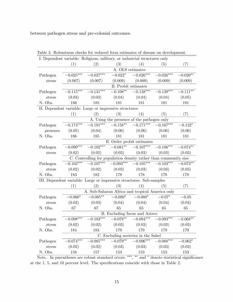
between pathogen stress and pre-colonial outcomes.

Table 3. Robustness checks for reduced form estimates of disease on development.

I. Dependent variable: Religious, military, or industrial structures only

(1) (2) (3) (4) (5) (7)

A. OLS estimates

Pathogen −0.025∗∗∗ −0.027∗∗∗ −0.022∗ −0.026∗∗∗ −0.026∗∗∗ −0.020∗∗stress (0.007) (0.007) (0.009) (0.009) (0.009) (0.009)

B. Probit estimates

Pathogen −0.115∗∗∗ −0.131∗∗∗ −0.108∗∗ −0.138∗∗∗ −0.139∗∗∗ −0.111∗∗stress (0.03) (0.03) (0.04) (0.04) (0.04) (0.05)

N. Obs. 186 185 181 181 181 181

II. Dependent variable: Large or impressive structures

(1) (2) (3) (4) (5) (7)

A. Using the presence of the pathogen only

Pathogen −0.174∗∗∗ −0.191∗∗∗ −0.158∗∗ −0.171∗∗∗ −0.167∗∗∗ −0.122∗presence (0.05) (0.04) (0.06) (0.06) (0.06) (0.06)

N. Obs. 186 185 181 181 181 181

B. Order probit estimates

Pathogen −0.099∗∗∗ −0.102∗∗∗ −0.081∗∗ −0.107∗∗∗ −0.106∗∗∗ −0.074∗∗stress (0.02) (0.02) (0.03) (0.03) (0.03) (0.03)

C. Controlling for population density rather than community size

Pathogen −0.102∗∗∗ −0.107∗∗∗ −0.093∗∗∗ −0.105∗∗∗ −0.103∗∗∗ −0.073∗∗stress (0.02) (0.02) (0.03) (0.03) (0.03) (0.03)

N. Obs. 183 182 178 178 178 178

III. Dependent variable: Large or impressive structures. Sub-samples

(1) (2) (3) (4) (5) (7)

A. Sub-Saharan Africa and tropical America only

Pathogen −0.060∗ −0.085∗∗ −0.080∗ −0.080∗ −0.07∗ −0.05stress (0.03) (0.03) (0.04) (0.04) (0.04) (0.04)

N. Obs. 67 67 65 65 65 65

B. Excluding Incas and Aztecs

Pathogen −0.098∗∗∗ −0.103∗∗∗ −0.078∗∗ −0.094∗∗∗ −0.093∗∗∗ −0.068∗∗stress (0.02) (0.02) (0.03) (0.03) (0.03) (0.03)

N. Obs. 184 183 179 179 179 179

C. Excluding societies in the Sahel

Pathogen −0.074∗∗∗ −0.085∗∗∗ −0.079∗∗ −0.096∗∗∗ −0.088∗∗∗ −0.062∗stress (0.02) (0.02) (0.03) (0.03) (0.03) (0.03)

N. Obs. 158 157 153 153 153 153

Note.— In parentheses are robust standard errors. ∗∗∗, ∗∗ and ∗ denote statistical significanceat the 1, 5, and 10 percent level. The specifications coincide with those in Table 2.

15

Finally, in panel III, I examine alternative sub-samples. I restrict the sample to tropical

areas only as a way to create a more meaningful comparison. I also exclude the Incas

and Aztecs from the sample to increase comparability, and even exclude sub-Saharan

African societies in the Sahel. In all these cases, the pattern observed in Table 2 remains

unaltered with only minimal changes in the point estimates. The only notable change is

in specifications (5) and (7) in panel III. In this set of regressions, which compare Africa

and tropical America, the estimate of becomes insignificant once an African indicator

is included. This is expected since the sample sizes are considerably smaller and the

variation in pathogen stress within the New World was limited.

Cities. The SCCS contains alternative measures of economic conditions but most

of them are difficult to validate.10 Anthropometric measures are also available but they

are not informative about comparative development.11 Archeological censuses of cities

are available and they can be used to corroborate the previous patterns. Archeological

censuses are not disaggregated at the level of societies but inventories of cities and their

sizes vary over time and so they complement the “snapshot” in the SCCS.

Table 4 reports the number of cities with populations over 20 and 40 thousand inhab-

itants in sub-Saharan Africa and tropical America, which, as I noted before, are quite

comparable regions. (There is no systematic information about tropical cities and towns

with less than 20 thousand inhabitants.) The inventory of cities comes from Chandler [17]

which, according to Connah [19], provides accurate patterns of city formation in Africa.

10The SCCS contains a very large number of variables (i.e., over two thousand variables) some which

could also serve as proxies for pre-colonial conditions. There are two limitations in using additional vari-

ables in the SCCS to assess pre-colonial development. First, one must be able to examine the SCCS data

against independent assessments in order to identify systematic errors and biases. The use of urbaniza-

tion in this subsection serves this purpose. Beyond urbanization, there seems to be no independent data

for many of the aspects coded in the SCCS including measures of political centralization. Second, a large

number of variables in the SCCS report information only about societies that are still present today. This

means that many of the variables have a large number of missing observations. Using these variables will

yield an incomplete (and perhaps incorrect) assessment of pre-colonial conditions.11By this I mean biological standards of living based on anthropometric measures such as height. In

particular, individuals in some African societies (i.e., the Tutsi) are exceptionally tall because height

is a genetic adaptation that helps diffuse heat. Individuals in other societies (i.e., the Pygmies), are

exceptionally short because they lack, due to genetic reasons, the growth spur during adolescence. Any

cross-sectional inference based on height would be uninformative because of the importance of these

genetic adaptations. In a separate line of inquiry, Ehret [27] used linguistic archaeology to trace out the

diffusion and origin of pre-colonial technologies but only for sub-Saharan Africa.

16

Table 4 reports different time periods and divides sub-Saharan Africa into three sub-

regions. The cities in regions with high Arab influence are coded as Muslims while the

Middle Nile and Ethiopia are regions likely influenced by ancient Egypt. The cities in the

rest of sub-Saharan Africa could be considered as “indigenous” though such classification

is not necessarily relevant for the analyses presented here.12 Table 4 shows that during

pre-Muslim times (i.e., 800), the number of medium- and large-sized cities in sub-Saharan

Africa, 5 and 1, was half of the number of cities in tropical America, 10 and 2. After 1200,

city formation changed rapidly in Africa due to the Arab-Muslim influence. In 1500, for

example, Africa and tropical America had an equal number of large cities.

Table 4. Cities in Africa and the New World.

Sub-Saharan Africa South

Year North Middle Nile North and Central

Africa Muslims and Ethiopia Rest Total America America

A. Number of cities with populations over 20,000 inhabitants

800 10 0 2 3 5 0 10

1000 13 0 1 4 5 0 9

1200 18 6 2 4 12 0 10

1300 18 8 2 5 15 0 11

1400 18 8 2 9 19 0 18

1500 19 13 3 8 24 1 16

B. Number of cities with populations over 40,000 inhabitants

800 4 0 0 1 1 0 2

1500 7 4 0 2 6 0 6

Note.— Data from Chandler ([17], pp. 39-57). The indigenous cities in sub-Saharan Africa

cover mostly Ghana, Zimbabwe and the Bantus. The middle Nile corresponds to Dongola

(modern Sudan) and Kaffa. North Africa includes cities in the Mediterranean (i.e., Arabian,

Egypt, Spanish Africa, and Aloa) and the Maghreb.

For comparative purposes, it is useful to note that the indigenous civilizations in South

12As Coquery-Vidrovitch ([20], p. 98) notes, cities in the area of Muslim influence “were more or

less Islamized throughout history, but they were certainly not historical ‘Muslim cities,’ except perhaps

Timbuktu.” Ancient Egypt apparently did not have a strong influence on sub-Saharan Africa although

cities appeared in the middle Nile earlier than in other areas. Meroë is the best known case. In 430 B.C.,

Meroë had about 20,000 inhabitants (Chandler [17], p. 461). Gold, ivory, slaves, and other mineral,

animal and vegetable products were traded with Eurasia through the Nubian corridor that connected

tropical Africa with Egypt. It has been suggested that this corridor was a cultural cul-de-sac, but such

description might be inaccurate; see Connah ([19], p. 19). There were also many ancient Swahili coastal

trading states in the eastern coast of Africa such as Kilwa; see Coquery-Vidrovitch ([20], Chapter 2).

17

and Central America originated in tropical rainforests similar to the African rainforest.

Moreover, none of their major cities were coastal and, in terms of latitude, their tropical

cities were close to the cities in sub-Saharan Africa. For example, the latitude of the main

cities of the Inca empire was about −13◦ and most Aztec cities were located at latitudesnear 20◦ to 22◦. In Africa, the ruins of the Great Zimbabwe are located at a latitude

of −20◦, while the cities of the Mali empire and predecessors (i.e., Djenné-Djenno, Gao,Kumbi Saleh), at a latitude of 15◦. The latitudes of Meroë and Aksum (in East Africa)

were 16◦ and 14◦. None of these cities were coastal. (An exception are the Swahili coastal

trading cities in the eastern coast; see footnote 12 for detailed references on city formation

in Africa.)

The previous inventory of cities has direct value but it also serves to estimate urban-

ization rates, which are perceived as more meaningful measures of pre-modern conditions;

see, e.g., Acemoglu et al. [2]. To measure urbanization rates, Table 5 reports demographic

data from Biraben [12] and McEvedy and Jones [45], which are independent sources.

Table 5. Pre-colonial population size in Africa and the Americas.

Biraben [12] McEvedy and Jones [45]

Region Area 400 BC AD 1000 1500 AD 1000 1500

Africa

North 2 10 14 9 9 8 11 8

Sub-Saharan 25 7 12 30 78 8 22 38

The Americas

North 20 1 2 2 3 0.4 0.7 1.3

South and Central 20 7 10 16 39 4 8 13

World population 153 252 253 461 170 265 425

Note.— Population in millions. Area (mill. km2) from McEvedy and Jones [45]. North Africa

includes the Maghreb, Libya and Egypt. The area in North Africa does not include the Sahara.

North America includes the US, Canada, and the Caribbean.

To construct the urbanization rate in sub-Saharan Africa, relative to tropical America,

I use the size of the urban population in Table 4 and the total population sizes in Table

18

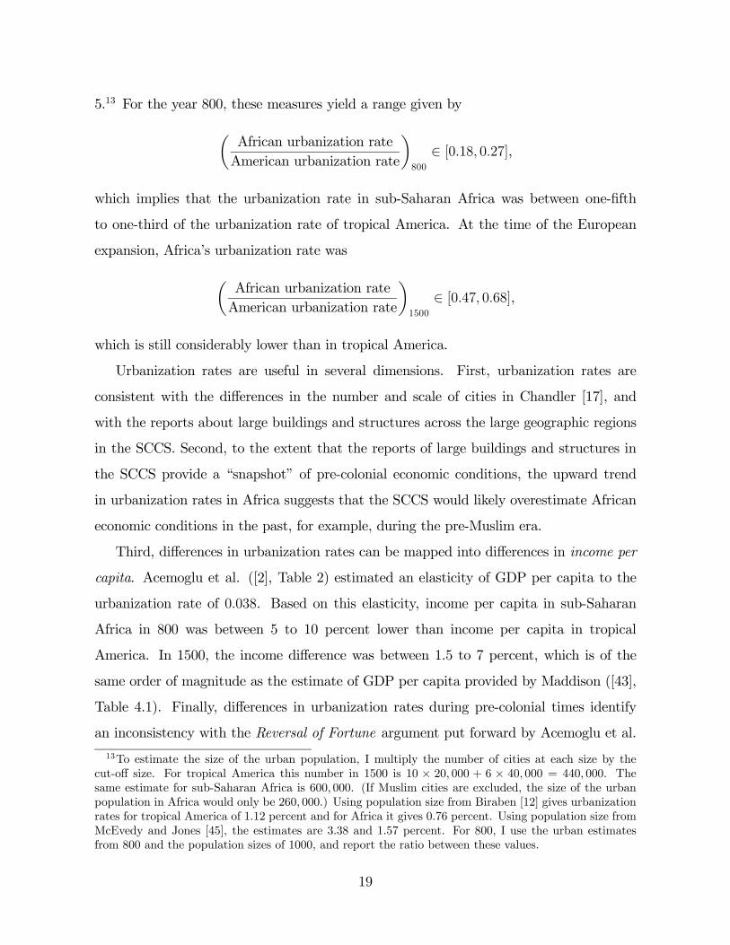
5.13 For the year 800, these measures yield a range given by

µAfrican urbanization rate

American urbanization rate

¶800

∈ [018 027],

which implies that the urbanization rate in sub-Saharan Africa was between one-fifth

to one-third of the urbanization rate of tropical America. At the time of the European

expansion, Africa’s urbanization rate was

µAfrican urbanization rate

American urbanization rate

¶1500

∈ [047 068],

which is still considerably lower than in tropical America.

Urbanization rates are useful in several dimensions. First, urbanization rates are

consistent with the differences in the number and scale of cities in Chandler [17], and

with the reports about large buildings and structures across the large geographic regions

in the SCCS. Second, to the extent that the reports of large buildings and structures in

the SCCS provide a “snapshot” of pre-colonial economic conditions, the upward trend

in urbanization rates in Africa suggests that the SCCS would likely overestimate African

economic conditions in the past, for example, during the pre-Muslim era.

Third, differences in urbanization rates can be mapped into differences in income per

capita. Acemoglu et al. ([2], Table 2) estimated an elasticity of GDP per capita to the

urbanization rate of 0038. Based on this elasticity, income per capita in sub-Saharan

Africa in 800 was between 5 to 10 percent lower than income per capita in tropical

America. In 1500, the income difference was between 1.5 to 7 percent, which is of the

same order of magnitude as the estimate of GDP per capita provided by Maddison ([43],

Table 4.1). Finally, differences in urbanization rates during pre-colonial times identify

an inconsistency with the Reversal of Fortune argument put forward by Acemoglu et al.

13To estimate the size of the urban population, I multiply the number of cities at each size by the

cut-off size. For tropical America this number in 1500 is 10 × 20 000 + 6 × 40 000 = 440 000. Thesame estimate for sub-Saharan Africa is 600 000. (If Muslim cities are excluded, the size of the urban

population in Africa would only be 260 000.) Using population size from Biraben [12] gives urbanization

rates for tropical America of 1.12 percent and for Africa it gives 0.76 percent. Using population size from

McEvedy and Jones [45], the estimates are 3.38 and 1.57 percent. For 800, I use the urban estimates

from 800 and the population sizes of 1000, and report the ratio between these values.

19

[2]. In particular, among former European colonies, Acemoglu et al. [2] found a strong

negative relationship between urbanization rates in 1500 and current income per capita.

The previous findings suggest that there has been no reversal in the ranking of economic

conditions in the tropical world, i.e., between sub-Saharan Africa and tropical America.14

In Acemoglu et al.’s [2] language, the findings imply that sub-Saharan Africa expe-

rienced a Persistence of Misfortunes: sub-Saharan Africa has remained relatively poor

compared to tropical America. This is not a contradiction of Acemoglu et al. [2]. Ace-

moglu et al. [2], for instance, explain why North America and Australia are richer than

tropical America and Africa. Their analysis, however, is not informative about why sub-

Saharan Africa still lags behind tropical America.

Since land areas are roughly the same (Table 5), Tables 1 and 5 also imply that

sub-Saharan Africa was more densely populated than tropical America, and almost as

densely populated as North Africa and Eurasia. This pattern seems to conflict with the

urbanization rankings. Population density, however, was not systematically associated

with urbanization and state consolidation in Africa.15 In all other regions of the world,

urbanization rates and population densities are strongly positively associated. Africa’s

distinct pattern has been previously documented in multiple independent analyses of po-

litical scientists; see, e.g., Fortes and Evans-Pritchard [32] and Vengroff [62]. In Appendix

A, I indeed verify that large and impressive structures are strongly positively associated

to population density in all regions of the world but sub-Saharan Africa. Appendix A

also discusses some of the main limitations of using population density as a measure of

pre-colonial sophistication.

14Acemoglu et al. ([2], Table 3 (1)) provides a point estimate of urbanization rates in 1500 on current

GDP per capita for former European colonies of −0078 (standard error 0.026). This estimate implies thatcurrent GDP per capita in Africa should be as much as 25 percent higher than in tropical America but

current differences in income per capita are of the order of 4:1 favoring Latin America. Their empirical

analysis of urbanization excluded sub-Saharan Africa arguing for measurement difficulties, although they

used data from Chandler [17] for other world regions.15Data on population density contradict Herbst [36], who argued that the lack of state consolidation in

pre-colonial Africa was a consequence of a relatively low population density. Herbst [36] argued that low

population density made state control more difficult and competition for space less attractive. Implicit

in Herbst [36] is a comparison between state formation in Africa and Europe. The comparison between

pre-colonial Africa and the Americas suggests a weaker link between state formation and population

densities. The Americas had smaller population densities than Africa but their independent development

of states resembles to an astonishing degree those patterns seen in the earliest states of Eurasia.

20

3 Disease, diversity, and development

Pathogen stress is negatively associated with the presence of large buildings and structures

during the pre-colonial era. This association is robust and consistent with independently

assessed measures of urbanization. Pathogen stress is primarily determined by environ-

mental conditions, so the previous association is likely the result of a causal process.

Obviously, such an association might simply be the reflection of omitted variables, mis-

specification errors, and/or measurement errors. Given the data limitations, it is not

possible to rule out any of these explanations. Another important shortcoming is the lack

of specific channels of causation. Pathogens could have a direct influence on pre-colonial

outcomes through, for example, a biological channel associated with reduced work energy;

see, e.g., Bloom and Sachs [15], Fogel [31], and Kamarck [39]. Pathogens could also have

an indirect influence on the social, economic, and political organization of society.16 This

section empirically examines an indirect mechanism based on the hypothesis that disease

limits economic development by increasing social fragmentation.

A causal process. The theoretical foundations for a causal process between disease

and diversity are spelled out in a separate paper, Birchenall [13]. The underlying logic,

however, is fairly simple: in settled agricultural societies, pathogen avoidance encourages

social fragmentation leading to more diverse populations.

Segregation due to disease is consistent with well-known social barriers. In fact, dis-

ease, as an isolating force in agrarian societies, is so common that social stigma is discussed

many times in the Old Testament.17 In another context, William McNeill argued that

parasitic disease in India lead to social segregation in the form of a rigid caste system.

McNeill ([46], pp. 66-67) argues that “the taboos on personal contact across caste lines,

16A well-known example of an indirect channel is the influence of disease on European settlements and

institutions studied by Acemoglu et al. [1]. The SCCS includes indigenous groups at the time of the

European arrival so, in principle, this channel has to be ruled out.17The Old Testament also tells the tale of the Tower of Babel, in which language diversity resulted in

the lack of large-scale coordination and communication. These discussions represent in a simple (but not

unique) way the general view proposed here. Other visible examples of social segregation that dealt with

disease during pre-modern times are public health quarantines and sanatoriums. Social segregation due

to disease is also present in nonhuman species as discussed by Kurzban and Leary ([40], p. 191). They

provide several examples of parasite avoidance in fish and social exclusion of polio-stricken chimpanzees.

21

and the elaborate rules for bodily purification in case of inadvertent infringement of such

taboos, suggests the importance fear of disease probably had in defining a safe distance

between the various social groups that became the castes of historic Indian society.” The

end result was that “the homogenizing process fell short of the ‘digestive’ pattern char-

acteristic of the other Old World civilizations. Consequently, the cultural uniformity and

sociological cohesion of the Indian peoples has remained relatively weak in comparison

to the more unitary structures characteristic of the northerly civilizations of Eurasia.”

India, for example, is the only non-African country with high levels of ethnolingusitic

fractionalization; see Easterly and Levine ([26], Table III).

Segregation is also consistent with the increased benefits of economic and geographic

isolation in high-disease areas. One social adaptation to disease was the tendency for

trade in pre-colonial Africa to be conducted at the border of territories, rather than at

centralized markets. Azevado ([8], p. 127) notes that: “[b]efore the European arrival

in the interior of central Africa, trade was localized and organized in such a way that

one ethnic group transported its goods to the limits of its district, and the next group

did the same.” As Curtin et al. ([22], pp. 93-94) noted, this pattern of exchange was

also common in the trans-Saharan trade networks as “aliens encountered severe health

problems in West Africa, and merchants tended to turn back at the deserts’ edge.”

Another adaptation to disease in tropical areas is the use of high altitude settlements.

High altitude settlements were characteristic of the Incas and Aztecs in the Americas,

whose capital cities were located in the interior and at high altitudes. High altitude

settlements, while protective against tropical diseases, increased transportation cost and

reduced incentives for trade and social integration. A number of studies have suggested

that mountains are frequently refuge areas that are difficult to conquer and integrate.

Indeed, Michalopoulos [47] has proposed an tested hypothesis to account for modern

ethnolinguistic fractionalization in Africa emphasizing land quality and elevation.18 In

18Particular case studies about the role of geography on the Nigerian highlands and the Liangshan

mountains between China and Tibet have been referenced by Cashdan ([16], p. 977). Disease also

limited trade in sub-Saharan Africa through a separate mechanism briefly discussed by Hull ([41], p.9):

“the tsetse fly, which attacked animals and rendered them unreliable as conveyors of goods. Consequently,

nearly everything had to be carried atop human heads. Transport was therefore expensive and enormously

22

Birchenall [13] I provide a complementary discussion of this and similar adaptations to

disease.

Finally, segregation due to disease is consistent with systematic studies of biologists

and anthropologists. For example, Cashdan [16] and Fincher and Thornhill [30] studied

the geographical patterns of ethnic group distributions and language in the world. They

concluded that environmental factors such as unpredictable climate, pathogen stress, and

habitat diversity shape ethnic diversity. In particular, Cashdan ([16], pp. 975-976) con-

cludes that “one of the strongest environmental predictors of high ethnic diversity is

pathogen stress” and that “this pattern of relationships suggests that pathogens may

be an important force in limiting the size of chiefdom/states.” Similarly, Fincher and

Thornhill ([30], p. 1289) conclude that “the worldwide distribution of indigenous human

language diversity is strongly positively related to human parasite diversity.”

Empirical estimates for disease and diversity in the SCCS. This subsection

documents a strong positive association between pathogen stress and pre-colonial ethnic

diversity. This association, driven primarily (but not exclusively) by African societies, can

be interpreted as causal under the assumption that disease is exogenous. Later in this

section I also show that there is a strong negative association between ethnic diversity

and state capacity (i.e., large buildings and structures). The nature of this relationship

is complicated because ethnic diversity and state capacity are both endogenous variables

and it is difficult to make causal claims. Later on in this section I provide some additional

remarks on this issue.

Figure 1 plots the number of ethnic groups within 500 miles of each agricultural society

in the SCCS against pathogen stress, across the main geographic regions studied here.

The figure shows a strong positive association between disease and ethnic diversity; more

ethnic groups are present in more disease-prone areas. The figure also shows that the

previous relationship is primarily (but not exclusively) driven by African societies.

Table 6 presents OLS estimates of equation (1) using the number of ethnic groups

within 500 miles as dependent variable, and similar specifications as Table 2. Overall,

inefficient.”

23

‐20

0

20

40

60

80

100

120

5 10 15 20 25

Number of ethnic groups within 500 m

Pathogen stress

Sub‐Saharan Africa Tropical America

Regression line (over all areas) Eurasia (including North Africa)

Figure 1: Pathogen stress and ethnic diversity in agricultural societies in the SCCS.

the relationship between pathogen stress and ethnic diversity is positive. Column (1)

includes no controls and shows that higher pathogen stress is associated with higher

ethnic diversity. The magnitude and significance of this effect is robust to the addition

of demographic controls in the form of community size, column (2). Community size

is an important control because measures of ethnic diversity in the SCCS are based on

physical distance. Column (3) controls for geographic factors such as latitude, altitude,

and agricultural potential. Latitude and altitude often play a significant role. For instance,

ethnic diversity is concentrated in tropical and mountainous areas. The point estimate

for disease declines in column (3) from 46 to 33, but the statistical significance of the

point estimates survives the inclusion of these geographic controls. This suggests that the

association between pathogen stress and diversity is not masking channels of geographic

variability previously studied by the literature; see, e.g., Michalopoulos [47]. Controlling

for food surplus and technological sophistication in the society, column (4), leaves the

24

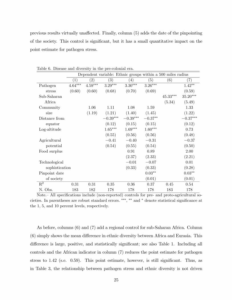
previous results virtually unaffected. Finally, column (5) adds the date of the pinpointing

of the society. This control is significant, but it has a small quantitative impact on the

point estimate for pathogen stress.

Table 6. Disease and diversity in the pre-colonial era.

Dependent variable: Ethnic groups within a 500 miles radius

(1) (2) (3) (4) (5) (6) (7)

Pathogen 4.64∗∗∗ 4.59∗∗∗ 3.29∗∗∗ 3.30∗∗∗ 3.26∗∗∗ 1.42∗∗

stress (0.60) (0.60) (0.68) (0.70) (0.69) (0.59)

Sub-Saharan 45.33∗∗∗ 35.20∗∗∗

Africa (5.34) (5.49)

Community 1.06 1.11 1.08 1.59 1.33

size (1.19) (1.21) (1.40) (1.45) (1.22)

Distance from −0.39∗∗∗ −0.39∗∗∗ −0.37∗∗ −0.37∗∗∗equator (0.12) (0.15) (0.15) (0.12)

Log-altitude 1.65∗∗∗ 1.69∗∗∗ 1.60∗∗∗ 0.73

(0.55) (0.56) (0.56) (0.48)

Agricultural −0.41 −0.40 −0.31 −0.37potential (0.54) (0.55) (0.54) (0.50)

Food surplus 0.91 0.89 2.00

(2.37) (2.33) (2.21)

Technological −0.01 −0.07 0.01

sophistication (0.33) (0.33) (0.28)

Pinpoint date 0.03∗∗ 0.03∗∗

of society (0.01) (0.01)

R2 0.31 0.31 0.35 0.36 0.37 0.45 0.54

N. Obs. 183 182 178 178 178 183 178

Note.— All specifications include (non-reported) controls for pre- and proto-agricultural so-

cieties. In parentheses are robust standard errors. ∗∗∗, ∗∗ and ∗ denote statistical significance atthe 1, 5, and 10 percent levels, respectively.

As before, columns (6) and (7) add a regional control for sub-Saharan Africa. Column

(6) simply shows the mean difference in ethnic diversity between Africa and Eurasia. This

difference is large, positive, and statistically significant; see also Table 1. Including all

controls and the African indicator in column (7) reduces the point estimate for pathogen

stress to 142 (s.e. 0.59). This point estimate, however, is still significant. Thus, as

in Table 3, the relationship between pathogen stress and ethnic diversity is not driven

25

exclusively by African societies or by the controls included in column (7). This observation

is important because Tables 1 and 6 show that the regional variation in ethnic diversity is

large. For example, the R2 in Table 6, column (6), suggests that the sub-Saharan African

control accounts for a considerable fraction of the total variation in ethnic diversity in

the world. Columns (6) and (7) also show that the set of controls in Table 6 account for

about 20 percent of Africa’s ethnic diversity, as measured by the decline in the African

indicator in column (7) relative to column (6); the African indicator declines by about 20

percent, from 45 to 35.

To assess the quantitative significance of disease, one can use the point estimates of

Table 6 and the difference in pathogen stress between Africa and tropical America, 373,

or the difference between Africa and Eurasia, 464. The point estimate for disease in

column (7), 142, the lowest point estimate in Table 6, implies that one should see about

53 and 65 more ethnic groups in Africa relative to the previous regions. Pathogen stress

thus accounts for about 11 and 14 percent of the baseline differences seen in Table 1. A

difficulty with Table 6, and therefore with the previous quantitative assessment, is that

the estimates of disease on diversity are not as “stable” as in Tables 2 and 3. The decline

in these point estimates as the number of controls increases suggests the presence of an

omitted variable correlated with disease and diversity. Given the large number of variables

assembled in the SCCS (see footnote 10), there is no limit to the controls one can add

to the previous specifications. Economic theory, however, suggests only a limited number

of potential determinants of ethnic diversity. I consider some of them in the sensitivity

analyses below.

Sensitivity analysis. This subsection examines the robustness of the previous find-

ings by paying special attention to alternative sub-samples and additional controls. I also

consider some more standard checks, such as those in Table 3. Panel I.A in Table 7,

for example, considers just the presence of the pathogens in the local environment. The

point estimate for disease follows the same pattern as in Table 6, but disease becomes

insignificant once the African indicator is included. (The p-value, however, is only 0.11

in column (7).) As in Table 6, column (7), the effects of disease weaken because most of

26

the variation in ethnic diversity happens to be between African and non-African regions,

and the African indicator absorbs most of this variation. Panels I.B and I.C show that

replacing community size for population density as a control has no effect on the point

estimates but restores significance in column (7), and that using the number of ethnic

groups in a 250 mile radius yields similar results.

Panel II in Table 7 studies several sub-samples. One of the most interesting compar-

isons is between tropical America and sub-Saharan Africa. The New World developed

independently from the Old World, and as I previously noted, tropical America and sub-

Saharan Africa shared many similarities in terms of technology and geography, but an

important asymmetry in their disease environments. Despite the large reduction in sam-

ple sizes, the point estimates of disease in this comparison (panel II.A) are larger and

more precisely estimated than in the benchmark cases of Table 6.

Sub-Saharan Africa had repeated contact with Eurasia through the Nile River, the

Sahara (by the Arab trade that started during the seventh century AD), and the Indian

ocean (by the East African trade in medieval times).19 Given their repeated interactions

before the European expansion, panel II.B considers a comparison between Eurasia and

sub-Saharan Africa. In this case, the effects of disease are also stronger than in Table 6.

The only sub-samples in which disease has no systematic effect on ethnic diversity

are those that include North and sub-Saharan Africa, and those that exclude tropical

Africa entirely, panels C and D. It is not accurate to state that disease does not matter

in these specifications. Disease has a positive effect on diversity even when demographic

controls are in place, columns (1) and (2). This positive effect, however, is accounted for

by the geographic, technological, and environmental factors included in columns (3) and

(4). Thus geographic, technological, and environmental factors that help explain ethnic

diversity in non-African societies are insufficient to account for Africa’s ethnic diversity.

19In fact, contact was enough to expose Africa to the epidemiological conditions of Eurasia. McNeill

([46], p. 130) noted that “when African slaves began to come to the new world after 1500, they suffered

no spectacular die-off from contact with European diseases, which is sufficient demonstration that in their

African habitat some exposure to the standard childhood diseases of civilization must have occurred.”

As Curtin et al. ([22], p. 242) note, even in the more distant regions, “the Bantu-speaking farmers of

southern Africa had some immunities to help protect them from the European diseases that exterminated

the indigenous people of Tasmania and decimated those of Patagonia.”

27

Table 7. Robustness checks for reduced form estimates of disease and diversity.

I. Dependent variable (for A and B): Ethnic groups within a 500 miles radius

(1) (2) (3) (4) (5) (7)

A. Using the presence of the pathogen only

Pathogen 7.58∗∗∗ 7.49∗∗∗ 4.78∗∗∗ 4.81∗∗∗ 4.72∗∗∗ 1.65

presence (1.15) (1.14) (1.25) (1.29) (1.26) (1.05)

B. Controlling for population density rather than community size

Pathogen 4.64∗∗∗ 4.64∗∗∗ 3.29∗∗∗ 3.38∗∗∗ 3.35∗∗∗ 1.55∗∗∗

stress (0.60) (0.59) (0.67) (0.68) (0.68) (0.59)

C. Using ethnic groups within a 250 miles radius as dependent var.

Pathogen 1.49∗∗∗ 1.47∗∗∗ 1.04∗∗∗ 1.05∗∗∗ 1.04∗∗∗ 0.50∗∗

stress (0.22) (0.22) (0.25) (0.26) (0.26) (0.22)

II. Dependent variable: Ethnic groups within a 500 miles radius. Sub-samples

(1) (2) (3) (4) (5) (7)

A. Sub-Saharan Africa and tropical America only

Pathogen 5.48∗∗∗ 5.26∗∗∗ 3.64∗∗∗ 3.42∗∗∗ 3.34∗∗∗ 1.69∗

stress (0.86) (0.87) (1.09) (1.12) (1.05) (0.93)

N. Obs. 67 67 65 65 65 65

B. Societies in the Old World

Pathogen 5.87∗∗∗ 5.80∗∗∗ 4.88∗∗∗ 5.13∗∗∗ 5.13∗∗∗ 2.82∗∗

stress (0.62) (0.61) (0.74) (0.73) (0.73) (0.78)

N. Obs. 118 117 113 113 113 113

C. Sub-Saharan and North Africa only

Pathogen 6.75∗∗∗ 6.49∗∗∗ 1.75 2.27∗ 2.30∗ 1.41

stress (1.20) (1.19) (1.26) (1.14) (1.17) (1.29)

N. Obs. 43 43 41 41 41 41

D. Non-African societies

Pathogen 1.40∗∗∗ 1.40∗∗∗ 0.37 0.33 0.35 0.35

stress (0.43) (0.44) (0.57) (0.55) (0.54) (0.54)

N. Obs. 151 150 148 148 148 148

III. Dependent variable: Ethnic groups within a 500 miles radius. Added controls

(1) (2) (3) (4) (5) (7)

A. Controlling for slavery

Pathogen 4.38∗∗∗ 4.33∗∗∗ 2.93∗∗∗ 2.95∗∗∗ 2.79∗∗∗ 1.34∗∗

stress (0.58) (0.58) (0.64) (0.66) (0.65) (0.56)

B. Controlling for political centralization

Pathogen 4.69∗∗∗ 4.64∗∗∗ 3.37∗∗∗ 3.36∗∗∗ 3.30∗∗∗ 1.50∗∗

stress (0.62) (0.62) (0.69) (0.69) (0.69) (0.60)

C. Controlling for large buildings and structures

Pathogen 4.50∗∗∗ 4.41∗∗∗ 3.19∗∗∗ 3.16∗∗∗ 3.16∗∗∗ 1.45∗∗

stress (0.58) (0.58) (0.65) (0.68) (0.67) (0.59)

Note.— In parentheses are robust standard errors. ∗∗∗, ∗∗ and ∗ denote statistical significanceat the 1, 5, and 10 percent level. The specifications coincide with those in Tables 2 and 6.

28

Omitted variables might still be unaccounted for. I next consider additional specifica-

tions that add controls that have been shown to be relevant for explaining ethnic diversity.

Panel III.A includes a control for the presence of slavery in the society.20 Slavery was prac-

ticed during pre-colonial times in Africa and it is a likely determinant of ethnic diversity.

As Nunn ([53], p. 164) noted, “slave trades tended to weaken the links between villages,

thus discouraging the formation of larger communities and broader ethnic identities.” The

effect of slavery (not reported) is often statistically significant but its inclusion does not

weaken the baseline estimates.

Linguistic, cultural, and ethnic fragmentation tend to disappear after the consolida-

tion of states; see, e.g., Weber [63].21 Food surplus and technological sophistication are

important determinants of state consolidation. They are indeed statistically significant

determinants of the presence and scope of large buildings and structures; see, columns (4),

(5), and (7) of Table 2. These variables, however, do not weaken the effect of disease on

diversity in the previous specifications. Panel III, specifications B and C, add controls for

political centralization and the presence of large buildings and structures. These controls

leave the baseline estimates of disease on diversity unaffected.

Finally, the effect of disease on ethnic diversity is primarily driven by sub-Saharan

Africa. It is thus possible that an “African factor” might be responsible for the previous

findings. A biased (i.e., Eurocentric) view of Africa or Africa’s long history relative to

other world regions are some examples of such “African factor.” (For instance, as Ashraf

and Galor [6] and Spolaore and Wacziarg [61] argue, Africa’s long history is likely re-

sponsible for Africa’s high genetic diversity and possibly its ethnic diversity.) To examine

this possibility, I consider the effect of disease on diversity in pre- and proto-agricultural

20A detailed analysis of slavery and forced labor during the pre-colonial era is beyond the scope of this

paper but it has been partly carried out by Patterson [56] for some societies in the SCCS. Patterson [56]

coded the presence and approximate origin of slave populations in the world. I use §v917 in the SCCS,as a control.21Weber ([63], p. 7), for example, noted in his analysis of state consolidation in France that “[d]iversity

had not bothered earlier centuries very much. It seem part of the nature of things, whether from place

to place or one social group to another. But the Revolution had brought with it the concept of na-

tional unity as an integral and integrating ideal at all levels, and the ideal of oneness stirred concern

about shortcomings. Diversity became imperfection, injustice, failure, something to be noted and to be

remedied.”

29

societies (i.e., hunter-gatherers). These societies are smaller in scale, less politically so-

phisticated, and geographically mobile so one should expect no effect of pathogenic stress

on diversity, i.e., pathogen avoidance is more easily achieved in small and mobile soci-

eties. If there is a built-in bias toward Africa or an “African factor,” one should also find

a significant African indicator for this hunter-gatherers.

Table 8. Disease and diversity in non—agricultural societies.

Dep. var.: Ethnic groups in 500 m.

(1) (2) (3)

Pathogen 0.15 −2.30stress (1.02) (1.66)

Sub-Saharan 27.16∗∗ 22.83

Africa (13.39) (17.10)

Full set of controls No No Yes

R2 0.00 0.08 0.25

N. Obs. 64 64 64

Note.— The sample is based on pre- and proto-agricultural societies. Full set of controls

corresponds to specification (7) in Table 6. In parentheses are robust standard errors. ∗∗∗, ∗∗

and ∗ denote statistical significance at the 1, 5, and 10 percent levels, respectively.

Table 8 presents three specifications. In (1), I control for disease but no other covariate,

in (2) I include an African indicator and no other control, and in (3) I control for all the

influences considered in the richest specification of Table 6. Sample sizes are small, but

column (1) finds no relationship between ethnic diversity and disease for non-agricultural

societies. There is, however, a significant difference in ethnic diversity between African and

non-African regions, column (2). The point estimate of the African indicator is smaller

than in Table 6 and its explanatory power and statistical significance are smaller. More

importantly, once the full set of controls is included, the African indicator and pathogen

stress both become insignificant. Thus there appears to be no systematic relationship

between disease and diversity for non-agricultural societies and no systematic difference

in ethnic diversity between non-agricultural societies in Africa and non-African regions.22

22These estimates also serve to discount systematic differences between Africa and non-African regions

due to sample selection and prejudice about Africa. For example, since most of the population movements

30

Empirical estimates for diversity and development in the SCCS. In modern

samples, ethnic, linguistic, religious, and cultural diversity have adverse effects of economic

outcomes and public policies; see, e.g., Alesina et al. [4], Ashraf and Galor [6], Bellows

and Miguel [10], Easterly and Levine [26], Miguel and Gugerty [50], and Spolaore and

Wacziarg [61]. This sub-section shows that there is a negative association between ethnic

diversity and the presence of large buildings and structures in the SCCS. The existing

literature often interprets this association as causal. In a long-term perspective, such

interpretation is not straightforward because ethnic diversity is endogenous.

Table 9. Large or impressive structures and ethnic diversity during the pre-colonial era.

Dependent variable: Large or impressive structures

(1) (2) (3) (4) (5) (7)

A. OLS correlations

Ethnic groups −0.008∗∗∗ −0.009∗∗∗ −0.006∗ −0.007∗∗ −0.006∗ 0.000

within 500 m. (0.003) (0.003) (0.003) (0.003) (0.003) (0.004)

R2 0.16 0.21 0.21 0.28 0.29 0.31

B. IV (second-stage)

Ethnic groups −0.021∗∗∗ −0.023∗∗∗ −0.027∗∗ −0.031∗∗∗ −0.031∗∗∗ −0.053∗within 500 m. (0.005) (0.005) (0.010) (0.010) (0.010) (0.031)

C. Augmented OLS

Ethnic groups −0.004 −0.004 −0.003 −0.003 −0.002 −0.002within 500 m. (0.03) (0.03) (0.03) (0.03) (0.03) (0.04)

Pathogen −0.081∗∗ −0.084∗∗∗ −0.078∗∗ −0.091∗∗ −0.092∗∗ −0.078∗∗stress (0.03) (0.03) (0.03) (0.03) (0.03) (0.03)

R2 0.18 0.23 0.23 0.31 0.32 0.33

N. Obs. 183 182 178 178 178 178

Note.— The instrumental variable strategy uses pathogen stress as instrument for ethnic

diversity. In parentheses are robust standard errors. ∗∗∗, ∗∗ and ∗ denote statistical significanceat the 1, 5, and 10 percent level. The specifications follow those of Tables 2 and 6.

I present three econometric specifications in Table 9 and discuss some statistical issues

about the interpretation of these estimates in Appendix B. These specifications rely on

in the long pre-agricultural period have been out of Africa, the sample of societies in Africa may be

a negatively selected sample of hunter-gatherers whereas the hunter-gatherers that migrated into the

Americas had positive attributes that later conduced to faster agricultural developments. Further, because

most of the societies in Africa were described at the peak of colonization, there may be prejudice against

African societies. The fact that there are no predictable differences between the non-agricultural societies

in Africa and the rest of the world suggests that prejudice and selection may not be crucial concerns.

31

the same set of controls as Tables 2 and 6. In particular, column (7) includes an African

indicator which is often statistically significant but whose value is not reported for con-

venience.23 First, panel A considers OLS correlations. Second, panel B considers an

instrumental variable strategy with pathogen stress as an instrument for ethnic diversity.

The validity of this strategy rests on two assumptions. Pathogen stress needs to be a

source of exogenous variation in ethnic diversity, which is a point demonstrated by Tables

6 and 7. More critically, conditional on the included controls, pathogen stress should

influence large or impressive structures only through ethnic diversity. This exclusion re-

striction is unlikely to hold because there are multiple unobserved influences of disease

on development. Thus there is an upward bias in an IV strategy. (I make this point

explicit in Appendix B.) Finally, panel C includes both ethnic diversity and pathogen

stress as predictors of large structures. There is a downward bias in this specification

due to over-controling because disease and diversity are strongly correlated. (I also make

this point explicit in Appendix B). These empirical strategies are likely biased in different

directions so they are complementary with no single one dominating the others.

Table 9 presents the results from the previous three specifications. In virtually all

instances, the point estimates of ethnic diversity on large buildings and structures are

negative. The OLS estimates are not distinguishable (statistically speaking) across speci-

fications and lose significance only once the African indicator is included. The IV estimates

are always significant. Moreover, the IV estimates are larger in absolute value than the

OLS correlations, and they become more negative as more controls are added, which is

expected given that there might be channels other than ethnic diversity through which

disease influenced economic outcomes in the past. Finally, despite the negative signs,

there are no significant point estimates for diversity once pathogen stress is included in

panel C. The point estimate for pathogen stress are marginally reduced relative to the

reduced-form estimates in Table 2. Both of these changes are expected given the pos-

itive effect of disease on ethnic diversity (Appendix B contains a formal discussion of

these points). Overall, Table 9 shows that there is a negative association between ethnic

23For convenience, I also do not report the point estimates for the controls. I also omit a number of

robustness checks (such as those of Tables 3 and 7) though they are available in Appendix C.

32

diversity and pre-colonial economic development. There are, however, large margins in

the previous estimates so the exact magnitude of the association between diversity and

development is difficult to pin down.24

4 The persistence of pre-modern influences

This section reports four empirical findings: (i) pathogen stress is negatively associated

with current income per capita, (ii) pathogen stress is positively associated with cur-

rent measures of ethnolinguistic fractionalization (from Easterly and Levine [26]), (iii)

pre-colonial ethnic diversity is negatively associated with current economic conditions

and positively associated with current ethnolingusitic fractionalization (ELF), and (iv)

pathogen stress is a central contributor to the mortality of European settlers during col-

onization, i.e., pathogen stress renders settler mortality insignificant as a predictor of the

current political institutions studied in Acemoglu et al. [2].

Data, merging, and additional controls. In order to link the SCCS to current

outcomes, I match each of the 186 societies to the countries where these societies located.

Appendix D lists the countries on which each society resided according to the latitude

and longitude provided by the SCCS. (To ensure a correct imputation, I used the Human

Relations Area Files, which separately lists the location of different cultures around the

world.) The matching of the SCCS to countries is fairly straightforward for agricultural

societies because there is limited geographic mobility in these societies. A concern is that,

sometimes, many societies locate in one country, and sometimes one society locates in

many countries. I allow for both possibilities and average SCCS variables across countries.

This concern is important because divided societies are more likely to experience civil wars

as noted by Michalopoulos and Papaioannou [49]. As a robustness check, I have also used

the country where the society is primarily located but the results are virtually identical.

24For example, the IV estimates in column (5) suggest a difference in large or impressive structures

between Africa and Eurasia of −0031 × (59 − 16) = −13, which is close to the actual difference, i.e.,−141 = 150−291; see Table 1. The OLS estimate in (5) suggests that ethnic diversity would account forabout one-fifth of the difference between these regions, and the augmented OLS estimate in (5) suggests

that ethnic diversity accounts for less than 10 percent of their difference.

33

Some societies, notably China, have been politically independent and unified for cen-

turies. For these societies, there is only a subtle distinction between pre-modern societies

and modern states. Other societies, notably the empires in the New World, were disinte-

grated by European influences. The use of modern income per capita thus requires special

care due to colonization. I control for colonial influences in three main ways. First, I focus

on former colonies only. This essentially restricts the sample to countries in Africa and

the New World, which has been an important comparison throughout the paper. Second,

I control for population densities in 1500 since they were arguably an important deter-

minant of colonial policies. Less densely populated colonies provided fewer incentives for

extractive institutions; see Acemoglu et al. [2]. Finally, I control for whether the country

was a British, French, German, Spanish, Italian, Dutch, or Portuguese colony. I also

add numerous controls associated with religion, natural endowments, and geography and

climate.25

Pathogen stress, current income per capita, and current ELF. Table 10

presents two sets of results. Panel A reports the reduced-form association between the

log of GDP per capita in 1995 and pathogen stress. This reduced-form regression are the

modern version of Tables 2 and 3. Panel A shows that pathogen stress has a negative

effect on income per capita. Controls for colonial influences, columns (2) and (3), weaken

the point estimate of pathogen stress but disease and current income per capita are still

negatively associated in these specifications. There is indeed a strong negative and statis-

tically significant reduced-form effect of pathogen stress on income per capita even after

the many additional controls for natural endowments and geography are in place. To gain

some perspective, there is a total of 28 controls in specification (6).

25Unless otherwise noted, I will rely on the variables coded by Acemoglu et al. ([2], Appendix 2) since

I want to explicitly minimize any interference introduced by including multiple variables from the SCCS.

I obtained all the data from their online Appendix. Religion includes controls for catholic, protestant,

muslim, and other. Endowments include mineral reserves associated with coal production, and measures

of natural reserves as percent of the world for gold, iron, silver, zinc, and oil. This set of controls also

includes whether a country is landlocked or an island. Geography controls for average temperature,

minimum monthly high, maximum monthly high, minimum monthly low, and maximum monthly low.

It also includes humidity variables associated with morning minimum, morning maximum, afternoon

minimum, and afternoon maximum as well as soil quality in the form of steppe (low latitude), steppe

(middle latitude), desert (middle latitude), dry steppe wasteland, desert dry winter, and highland. In

total, the richest specification has 28 controls.

34

Table 10. Income per capita, disease, and ethnolinguistic fragmentation.

(1) (2) (3) (4) (5) (6)

A. Dependent variable: Current log-GDP per capita

Pathogen −0.219∗∗∗ −0.161∗∗∗ −0.130∗∗∗ −0.135∗∗∗ −0.108∗∗∗ −0.084∗∗stress (0.026) (0.027) (0.033) (0.033) (0.040) (0.044)

R2 0.43 0.54 0.63 0.65 0.73 0.80

N.Obs/N.controls 67/1 66/2 66/10 65/12 65/20 65/28

B. Dependent variable: Current ethnolinguistic fractionalization (ELF)

Pathogen 0.035∗∗∗ 0.037∗∗∗ 0.030∗∗∗ 0.032∗∗∗ 0.034∗∗ −0.008stress (0.009) (0.011) (0.011) (0.011) (0.014) (0.016)

R2 0.13 0.14 0.34 0.41 0.57 0.68

N.Obs/N.controls 71/1 68/2 68/9 68/12 68/20 68/28

Controls included

Pop. density 1500 No Yes Yes Yes Yes Yes

Colonizer id. No No Yes Yes Yes Yes

Religion No No No Yes Yes Yes

Endowments No No No No Yes No

Geography No No No No No Yes

Note.— In parentheses are robust standard errors. ∗∗∗, ∗∗ and ∗ denote statistical significanceat the 1, 5, and 10 percent level. For variable definitions please see the main text, specially

footnote 25.

Panel B uses the average of five different indices of ethnolinguistic fractionalization

from Easterly and Levine [26], as used in Acemoglu et al. [1]. These regressions are

the modern version of Tables 6 and 7. Panel B shows three things: first, the influence

of pathogen stress on ELF is positive and statistically significant, with the exception

of specification (6) in which pathogen stress is not significantly different from zero (for

reasons that I briefly discuss later on). Second, in all other specifications, the point

estimate for pathogen stress is remarkable stable. Table 10, panel B, thus suggests that

pathogen stress is important for understanding current ethnic fragmentation and that

the effects of disease were not drastically perturbed by colonial influences. Third, an

important component of ethnolingusitic fragmentation is environmentally determined and

specification (6) has a large number of environmental controls relative to the number of

observations. Thus including temperature, humidity, latitude and similar variables render

pathogen stress insignificant because there is a strong correlation between these exogenous

factors, the severity of pathogen stress, and ethnic fragmentation.

35

Recall from Table 1 that the difference in pathogen stress in sub-Saharan Africa and

tropical America is 373 = 1746− 1373. This difference changes little once the societieshave been matched to actual countries. (For instance, the difference at the country level

is 33 = 1688 − 1358.) The log-income per capita gap between both regions in the

sample is −105 = ln($4 478) − ln($1 564). Using the OLS point estimate of panel

A, column (6), the lowest point estimate in the table, gives a predicted difference of

−0084 × 373 = −031. This difference is about 30 percent of the actual difference

between both regions, which is a large value especially since I have already considered

some competing explanations. For example, as I have controlled for colonizer identities

and population density in 1500, the estimates already take into account potential colonial

influences associated with differential colonial policies and the Reversal of Fortune studied

by Acemoglu et al. [2]. I have also controlled for religion, natural endowments, and

geography and climate. In fact, the R2 in the richest specification is about 80 percent.26

Appendix C considers several alternative specifications. I use the presence of the

previously listed pathogens discounting their severity and endemicity. I also add controls

for food surplus and technological sophistication based on the SCCS data. The findings

of Table 10 remain unchanged in these specifications. I also expand the sample to include

non-colonies, and find that pathogen stress plays a larger role on income per capita and

ethnic fragmentation in this specification. In other checks, I excluded sub-Saharan Africa

from the sample. None of the results are significant, which is consistent with the discussion

of the previous section. Sub-Saharan Africa is the most important source of variation in

pathogen stress and ethnic diversity or ethnolinguistic fractionalization in the data. Thus

excluding this region renders most estimates insignificant. Even a contrast between North

Africa and sub-Saharan, however, often yields strong and significant results. Finally, I

include countries in tropical America and Africa only. In this case, the point estimates

are also often negative and significant as in Table 10.

Ethnic diversity, current income per capita, and current ELF. Table 11

26I cannot directly control for urbanization which is a more precise measure of pre-colonial conditions

in Acemoglu et al. [2]. The measures of urbanization previously developed for sub-Saharan Africa apply

to the entire area and do not vary within Africa. One of the robustness checks in Appendix C adds large

or impressive structures as a control. This leaves the main results of Table 10 intact.

36

presents three sets of results: panel IA reports OLS correlations between GDP per capita

and pre-colonial ethnic diversity. Panel IB reports the same correlations but with current

ELF instead of the pre-colonial measure. The correlations between income and ELF are

well-known (Easterly and Levine [26]) but the general change in the point estimates in

Panel B provides a useful benchmark for Panel A. Finally, panel II reports OLS correla-

tions between pre-colonial ethnic diversity and current ELF.

Table 11. Income per capita, ethnolinguistic fractionalization, and ethnic diversity.

I. Dependent variable: Current log-GDP per capita

(1) (2) (3) (4) (5) (6)

A. Pre-colonial ethnic diversity

Ethnic groups −0.019∗∗∗ −0.014∗∗∗ −0.009∗∗ −0.010∗∗ −0.004 −0.003within 500 m. (0.003) (0.003) (0.004) (0.004) (0.004) (0.004)

R2 0.23 0.47 0.57 0.59 0.70 0.79

N.Obs/N.controls 67/1 66/2 66/10 65/12 65/20 65/28

B. Current ethnolinguistic fractionalization

Ethnolinguistic −1.382∗∗∗ −1.264∗∗∗ −1.083∗∗∗ −1.119∗∗∗ −0.838∗∗∗ −0.783∗∗fractionalization (ELF) (0.31) (0.26) (0.28) (0.30) (0.28) (0.33)

R2 0.18 0.50 0.58 0.58 0.70 0.75

N.Obs/N.controls 87/1 85/2 85/9 85/12 84/20 84/28

II. Dependent variable: Current ethnolinguistic fractionalization (ELF)

(1) (2) (3) (4) (5) (6)

Ethnic groups 0.66∗∗∗ 0.77∗∗∗ 0.65∗∗∗ 0.66∗∗∗ 0.60∗∗∗ 0.45∗∗∗

within 500 m. (×100) (0.07) (0.08) (0.09) (0.09) (0.12) (0.10)

R2 0.32 0.37 0.51 0.56 0.64 0.71

N.Obs/N.controls 71/1 68/2 68/9 68/12 68/20 68/28

Controls included

Pop. density 1500 No Yes Yes Yes Yes Yes

Colonizer id. No No Yes Yes Yes Yes

Religion No No No Yes Yes Yes

Endowments No No No No Yes No

Geography No No No No No Yes

Note.— In parentheses are robust standard errors. ∗∗∗, ∗∗ and ∗ denote statistical significanceat the 1, 5, and 10 percent level. For variable definitions please see the main text, specially

footnote 25.

Ethnic diversity and income per capita are endogenous variables so a causal assess-

ment of their relationship is difficult. Table 11, panels A and B, shows that diversity is

37

negatively correlated with income per capita. The correlation between pre-colonial ethnic

diversity and income is weaker than the correlation between current ELF and income.

The general pattern in panels A and B, however, is similar in the sense that the addi-

tion of controls weakens these correlations. For example, the point estimates in panel A

decline as the endowments and geographic controls are added; specifications (5) and (6)

are not statistically significant. One difference between these panels is that panel A has

considerably fewer observations compared to panel B. For instance, as Appendix C shows

(Table C4, panel C), if non-colonies are added to the sample in Table 11, pre-colonial

ethnic diversity remains significant even in the richest specifications.27

Panel II provides a more compelling view of the role of pre-colonial diversity on cur-

rent outcomes. This panel shows that pre-colonial and current measures of diversity are

strongly positively related and that their relationship is stable across specifications. This

means that colonization did not drastically alter the role of pre-colonial influences on

current diversity. For instance, if the current high levels of ethnic fragmentation in Africa

were solely due to colonial factors, one should see a marked decline in the point estimates

in panel II, columns (2) and (3). Likewise, religion, endowments, and geographic factors

do not lead to a decline in the point estimate for ethnic diversity. Table 11 thus shows

that pre-colonial diversity is associated with current outcomes though its effects are more

likely to be channeled through ELF rather than as a direct influence on income per capita.

Pathogen stress and colonial origins. The colonial origins hypothesis proposed

by Acemoglu et al. [1] considers a competing causal path through which disease lowers

income per capita. Briefly stated, this hypothesis argues that disease, as measured by

the mortality rates of potential European settlers, influences current outcomes through

27This significance of pre-colonial diversity on current income per capita once non-colonies are added

to the sample could be due simply to larger sample sizes or to the fact that past ethnic diversity is more

important for non-colonies than for European colonies. For instance, a homogenous population during

pre-modern times might be an important determinant of modern economic growth; see, e.g., Ashraf

and Galor [6] and Spolaore and Wacziarg [61] for discussions centered on the role of genetic diversity

on current economic outcomes. Separately, Appendix C instruments pre-colonial ethnic diversity with

pathogen stress (as in Table 9, panel B) and also finds larger and more significant effects. There is no need

to emphasize the IV strategy because this strategy is likely upward-biased, as discussed in Appendix B.

Appendix C also uses, for robustness, measures of ethnic diversity based on the number of ethnic groups

within a 250 miles radius and several other checks. In general, the point estimates change in the same

way as in the main tables, but all specifications yield negative and often significant results.

38

their effect on European settlements and institutions.28 This subsection briefly shows that

pathogen stress in the SCCS was an important component behind the mortality faced by

European settlers, and that its inclusion as a determinant of current institutions renders

settler mortality insignificant.

Table 12. Protection against expropriation risk, settler mortality, and pathogen stress.

(1) (2) (3) (4) (5) (6)

Dependent variable: Protection against expropriation risk

Pathogen stress −0.361∗∗∗ −0.327∗∗∗ −0.257∗∗∗ −0.242∗∗∗(0.046) (0.059) (0.068) (0.069)

Settler mortality −0.646∗∗∗ −0.654∗∗∗ −0.238 −0.234(0.125) (0.152) (0.179) (0.197)

Linked to SCCS No Yes Yes Yes Yes Yes

Country in AJR Yes Yes No Yes Yes Yes

Only colonies No No No No No Yes

R2 0.30 0.29 0.42 0.40 0.42 0.38

N. Obs. 74 58 81 58 58 54

Note.— In parentheses are robust standard errors. ∗∗∗, ∗∗ and ∗ denote statistical significanceat the 1, 5, and 10 percent level. Linked to SCCS means that at least one society in the SCCS

resided in the country. Country in AJR means that the country is part of the sample studied

by Acemoglu et al. [1]. Only colonies means that the country is a former European colony.

Table 12 examines the influence of disease on the protection against expropriation

risk. Column (1) includes settler mortality on the baseline sample of Acemoglu et al. [1].

Column (2) presents the same estimate for the 58 countries with data on settler mortality

also linked to the SCCS. The point estimate in both columns is virtually identical and

consistent with Acemoglu et al. ([1], Tables 3-6). Columns (3) and (4) show that the

sample in which pathogen stress and settler mortality are both available is representative.

More importantly, column (5) shows that when both pathogen stress and settler mortality

are included as predictors of protection against expropriation risk, the value of settler

mortality becomes insignificant. Column (6) in turn shows that restricting the sample

28A modified view, proposed by Glaeser et al. [34], argues that European settlements also influenced

human capital and not exclusively political institutions. Both views, however, place the influence of

disease during colonization at the center stage of current economic disparities.

39

to former colonies has no effect on the previous estimates. Table 12 thus shows that

pathogen stress is a better predictor of current institutions than settler mortality. It also

implies, in conjunction with previous findings, that disease matters for current economic

outcomes but not only through the selective penetration of European settlers, as stated

in the colonial origins hypothesis.

5 Final remarks

This paper empirically assessed the influence of disease on long-term comparative eco-

nomic development focusing on the influence of pathogen stress on pre-colonial state

consolidation in sub-Saharan Africa. To measure the state’s capacity to generate, ex-

tract, and mobilize resources in a society, I used the complexity of large or impressive

structures in the Standard Cross-Cultural Sample, a rich ethnographic account of pre-

industrial societies described at the time of first contact with Westerners. Ethnographic

data suggests that adverse disease environments limited the pace at which small-scale

societies developed into large-scale tributary empires and states in Africa.

This paper argued that these effects are present partly because parasitic diseases,

highly prevalent in tropical Africa due to environmentally given reasons, trigger repro-

ductive, social, and cultural isolation between human populations. Evidence of this causal

mechanism includes William McNeill’s historical analysis (McNeill [46]) as well as many

studies by social scientists discussed and analytically formalized in a companion paper

(Birchenall [13]). In the ethnographic data, high disease prevalence is associated with

high levels of ethnic diversity. This association is also robust across specifications and

controls, but the effects of disease on the social organization of pre-colonial societies tend

to be concentrated in sub-Saharan Africa. The effects of disease on economic develop-

ment and ethnic diversity are quite persistent and remain relevant even once many relevant

controls for colonial influences are taken into account. Tentatively, these findings suggest

that Africa’s slow transition into modern economic growth has some deep roots in its

pre-colonial past.

40

References

[1] Acemoglu, D., Johnson, S., and Robinson, J.A. (2001) “The Colonial Origins of

Comparative Development: An Empirical Investigation,” American Economic Re-

view, Vol. 91, 1369-1401.

[2] Acemoglu, D., Johnson, S., and Robinson, J.A. (2002) “Reversal of Fortune: Geog-

raphy and Institutions in the Making of the Modern World Income Distributions,”

Quarterly Journal of Economics, Vol. 107, 1231-1294.

[3] Acemoglu, D., Johnson, S., and Robinson, J.A. (2003) “An African Success Story:

Botswana,” in Rodrik D. (Ed.) In Search of Prosperity: Analytic Narratives

on Economic Growth, Princeton University Press, 80-122.

[4] Alesina, A., Devleeschauwer, A., Easterly, A., Kurlat, S., and Wacziarg, R. (2003)

“Fractionalization,” Journal of Economic Growth, Vol. 8, 155-194.

[5] Ashraf, Q. and Galor, O. (2011) “Dynamics and Stagnation in the Malthusian

Epoch,” American Economic Review, Vol. 101, 2003-2041.

[6] Ashraf, Q. and Galor, O. (2013) “The ‘Out of Africa’ Hypothesis, Human Genetic

Diversity, and Comparative Economic Development,” American Economic Review,

Vol. 103, 1-46.

[7] Austen, R.A. (1987) African Economic History: Internal Development and

External Dependency, James Currey.

[8] Azevado, M.J. (1980) “Epidemic Disease among the Sara of Southern Chad, 1890-

1940,” in Hartwig, G.W. and Patterson, K.D., Disease in African History, Duke

University Press, 119-152.

[9] Bates, R.H., Coatsworth, J.H., and Williamson, J.G. (2007) “Lost Decades: Postin-

dependence Performance in Latin America and Africa,” Journal of Economic History,

Vol. 67, 917-943.

41

[10] Bellows, J. and Miguel, E. (2009) “War and Local Collective Action in Sierra Leone,”

Journal of Public Economics, Vol. 93, 1144-1157.

[11] Bhattacharyya , S. (2009) “Root Causes of African Underdevelopment,” Journal of

African Economies, Vol. 18, 745-780.

[12] Biraben, J-N. (1979) “Essai sur L’évolution du Nombre des Hommes,” Population,

Vol. 34, 13-25.

[13] Birchenall, J.A. (2014) “A Theory of Disease and Development,” UCSB Mimeo.

[14] Bockstette, V., Chanda, A., and Putterman, L. (2002) “States and Markets: The

Advantage of an Early Start,” Journal of Economic Growth, Vol. 7, 347-369.

[15] Bloom, D.E. and Sachs, J. (1998) “Geography, Demography, and Economic Growth

in Africa,” Brookings Papers on Economic Activity, Economic Studies Program, Vol.

29, 207-296.

[16] Cashdan, E. (2001) “Ethnic Diversity and its Environmental Determinants: Effects

of Climate, Pathogens, and Habitat Diversity,” American Anthropologist, Vol. 103,

968-991.

[17] Chandler, T. (1987) Four Thousand Years of Urban Growth: An Historical

Census, St. Davis University Press.

[18] Collier, P. and Gunning, J.W. (1999) “Explaining African Economic Performance,”

Journal of Economic Literature, Vol. 37, 64-111.

[19] Connah, G. (2001) African Civilizations: An Archaeological Perspective,

Cambridge University Press.

[20] Coquery-Vidrovitch, C. (2011) The History of African Cities South of the

Sahara: From the Origins to Colonization, Wiener: Princeton.

[21] Crosby, A.W. (2003)The Columbian Exchange: Biological and Cultural Con-

sequences of 1492, Greenwood Publishing Group.

42

[22] Curtin, P., Feierman, S., Thompson, L., and Vansina, J. (1995) African History:

From Earliest Times to Independence, Longman: New York.

[23] Davidson, B. (1959) The Lost Cities of Africa, Little, Brown and Company.

[24] Diamond, J. (1997) Guns, Germs and Steel: The Fates of Human Societies,

Vintage.

[25] Diamond, J. and Panosian, C. (2006) “Continental Asymmetry of the Origins of Hu-

man Infectious Diseases,” in Hämäläinen, P. (Ed.)When Disease Makes History:

Epidemics and Great Historical Turning Points, Helsinki Univ. Press, 17-44.

[26] Easterly, W. and Levine, R. (1997) “Africa’s Growth Tragedy: Policies and Ethnic

Divisions,” Quarterly Journal of Economics, Vol. 112, 1203-1250.

[27] Ehret, C. (1998) An African Classical Age: Eastern and Southern Africa in

World History, 1,000 B.C. to A.D. 400, University of Virginia Press.

[28] Englebert, P. (2000) State Legitimacy and Development in Africa, Lynne Ri-

enner Publishers.

[29] Fenske, J. (2014) “Ecology, Trade, And States In Pre-Colonial Africa,” Journal of

the European Economic Association, Vol. 12(3), 612-640.

[30] Fincher, C.L. and Thornhill, R. (2008) “A Parasite-drivenWedge: Infectious Diseases

may Explain Language and other Biodiversity,” Oikos, Vol. 117, 1289 1297.

[31] Fogel, R. (1994) “Economic Growth, Population Theory, and Physiology: The Bear-

ing of Long-Term Processes on the Making of Economic Policy,” American Economic

Review, Vol. 84, 369-395.

[32] Fortes, M. and Evans-Pritchard, E.E. (1940) African Political Systems, Oxford

University Press.

[33] Gennaioli, N. and Rainer, I. (2007) “The Modern Impact of Precolonial Centraliza-

tion in Africa,” Journal of Economic Growth, Vol. 12, 185-234.

43

[34] Glaeser, E.L., La Porta, R., Lopez-de-Silanes, F., and Shleifer, A. (2004) “Do Insti-

tutions Cause Growth?,” Journal of Economic Growth, Vol. 9, 271-303.

[35] Heldring, L. and Robinson, J.A. (2012) “Colonialism and Economic Development in

Africa,” NBER Working Paper No. 18566.

[36] Herbst, J. (2000) States and Power in Africa: Comparative Lessons in Au-

thority and Control, Princeton University Press.

[37] Hoeppli, R. (1969) “Parasitic Diseases in Africa and the Western Hemisphere: Early

Documentation and Transmission by the Slave Trade,” Acta Tropica, Supplementum

No. 10.

[38] Hopkins, A.G. (1973) An Economic History of West Africa, Columbia Univer-

sity Press.

[39] Kamarck, A. (1967) The Economics of African Development, Praeger Publish-

ers.

[40] Kurzban, R. and Leary, M.R. (2001) “Evolutionary Origins of Stigmatization: the

Functions of Social Exclusion,” Psychological Bulletin, Vol. 127, 187-208.

[41] Hull, R.W. (1976) African Cities and Towns before the European Conquest,

W.W. Norton.

[42] Low, B.S. (1990) “Marriage Systems and Pathogen Stress in Human Societies,”

American Zoologist, Vol. 30, 325-339.

[43] Maddison, A. (2001) The World Economy: A Millennial Perspective, OECD

Development Centre.

[44] Mann, C.C. (2005) 1491: NewRevelations of the Americas Before Columbus,

Alfred A. Knopf.

[45] McEvedy, C. and Jones, R. (1985) Atlas of World Population History, Penguin

Books.

44

[46] McNeill, W.H. (1976) Plagues and People, Anchor Books.

[47] Michalopoulos, S. (2012) “The Origins of Ethnolinguistic Diversity,” American Eco-

nomic Review, Vol. 102, 1508-1539.

[48] Michalopoulos, S. and Papaioannou, E. (2013) “Pre-Colonial Ethnic Institutions and

Contemporary African Development,” Econometrica, Vol. 81, 113-152.

[49] Michalopoulos, S. and Papaioannou, E. (2013) “The Long-Run Effects of the Scram-

ble for Africa,” NBER Working Paper No. 17620.

[50] Miguel, E. and Gugerty, M.K. (2005) “Ethnic Diversity, Social Sanctions, and Public

Goods in Kenya,” Journal of Public Economics, Vol. 89., 2325-2368.

[51] Murdock, G.P. (1967) Ethnographic Atlas, University of Pittsburgh Press.

[52] Murdock, G.P. and White, D.R. (1969) “Standard Cross-Cultural Sam-

ple,” Ethnology, Vol. 9, 329-369. Updates are available online at

http://repositories.cdlib.org/imbs/socdyn/wp/Standard_Cross-Cultural_Sample

[53] Nunn, N. (2008) “The Long-Term Effects of Africa’s Slave Trades,”Quarterly Journal

of Economics, Vol. 123, 139-176.

[54] Nunn, N. and Wantchekon, L. (2011) “The Slave Trade and the Origins of Mistrust

in Africa,” American Economic Review, Vol. 101, 3221-3252.

[55] Osafo-Kwaako, P. and Robinson, J. (2013) “Political Centralization in pre-Colonial

Africa,” Journal of Comparative Economics, Vol. 41, 6-21.

[56] Patterson, O. (1982) Slavery and Social Death: A Comparative Study, Har-

vard University Press.

[57] Price-Smith, A.T. (2008) Contagion and Chaos: Disease, Ecology, and Na-

tional Security in the Era of Globalization, MIT press.

45

[58] Pryor, F.L. (2005) Economic Systems of Foraging, Agricultural, and Indus-

trial Societies, Cambridge University Press.

[59] Rosen, W. (2007) Justinian’s Flea: Plague, Empire, and the Birth of Europe,

Penguin.

[60] Smith, B.D. (1995) The Emergence of Agriculture, Scientific American Library.

[61] Spolaore, E. and Wacziarg, R. (2009) “The Diffusion of Development,” Quarterly

Journal of Economics, Vol. 124, 469-529.

[62] Vengroff, R. (1976) “Population Density and State Formation in Africa,” African

Studies Review, Vol. 19, 67-74.

[63] Weber, E. (1976) Peasants into Frenchmen: The Modernization of Rural

France, 1870-1914, Stanford University Press.

[64] Wolfe, N.D., Dunavan, C.P., and Diamond, J. (2007) “Origins of Major Human

Infectious Diseases,” Nature, Vol. 447, 279-283.

[65] Zinsser, H. (1935) Rats, Lice and History, Little, Brown and Company.

46

6 Appendix A: Population density and urbanization

During the pre-colonial era, sub-Saharan Africa was more densely populated than tropical

America. Yet, urbanization rates were lower and large and impressive structures were

less prevalent in Africa than in any other region. This Appendix demonstrates that

African development followed a divergent pattern for urbanization by showing that in all

other world regions in the SCCS, large and impressive structures are strongly positively

associated with population density. In sub-Saharan Africa, these variables are statistically

independent. This Appendix also provides additional remarks about this pattern and the

use of population density to measure economic conditions during the pre-colonial era.

Table A1. OLS correlation between large or impressive structures and population density.

Tropical

All Sub-Saharan Non-African Tropical America

societies Africa societies Eurasia America (no empires)

(1) (2) (3) (4) (5) (6)

I. Dependent variable: Large or impressive structures

Population 0.22∗∗∗ −0.29 0.28∗∗∗ 0.23∗∗∗ 0.37∗∗∗ 0.30∗

density (0.05) (0.23) (0.05) (0.07) (0.12) (0.15)

R2 0.20 0.14 0.30 0.27 0.35 0.29

II. Dependent variable: Religious, military, or industrial structures only

Population 0.06∗∗∗ −0.05 0.08∗∗∗ 0.07∗∗∗ 0.13∗∗∗ 0.10∗∗

density (0.01) (0.05) (0.01) (0.02) (0.03) (0.04)

R2 0.12 0.10 0.16 0.13 0.35 0.26

N. Obs. 184 32 152 118 34 32

Note.— No empires means that the Incas and Aztecs have been excluded. All specifications

include a (non-reported) control for pre- and proto-agricultural societies. In parentheses are

robust standard errors. ∗∗∗, ∗∗ and ∗ denote statistical significance at the 1, 5, and 10 percentlevel.

Table A1, panel I, shows that there is no systematic association between population

density and the presence of large buildings and impressive structures in Africa. Panel II

shows the same results for the presence of religious, military, or industrial structures only.

These results contrast with a positive association in all other agricultural societies in the

world. Specifically, column (1) of Table A14 reports the OLS correlation between the

47

presence of large buildings and population density in all societies. Column (2) examines

the same correlation within Africa. This correlation is actually negative although not

statistically significant. In non-African regions, this correlation is strong and positive,

column (3). This is also true for societies in Eurasia, column (4). In tropical America, the

correlation is actually stronger than in non-African societies, column (5), and not solely

driven by the presence of large empires such as the Incas and the Aztecs, column (6).

The pattern documented in Table A1 has also been evident to African political scien-

tists. Fortes and Evans-Pritchard ([32], pp. 7-8), for example, in discussing the influence

of demography on African political systems, noted that

“it would be incorrect to suppose that governmental institutions are found

in those societies with greatest [population] density. The opposite seems to

be equally likely, judging by our material. The density of the Zulu is 3.5, of

the Ngwato 2.5, of the Bemba 3.75 per square mile, while that of the Nuer is

higher and of the Tallensi and Logoli very much higher. It might be supposed

that the dense permanent settlements of the Tallensi would necessarily lead

to the development of a centralized form of government, whereas the wide

dispersion of shifting villages among the Bemba would be incompatible with

centralized rule. The reverse is actually the case. In addition to the material

collected in this book, evidence from other African societies could be cited to

prove that a large population in a political unit and a high degree of political

centralization do not necessarily go together with great density.”

Population density provides a poor indication of political centralization in Africa. Pop-

ulation density might also be a poor proxy for economic conditions in the pre-colonial era.

Acemoglu et al. [2] provide several reservations regarding the use of population density

as a proxy for pre-modern conditions. The current empirical link between population

density and income per capita is weaker than that of urbanization. For instance, there is

no cross-sectional association between population density and income per capita today.

This means that differences in population density during the pre-colonial era cannot be

48

transalted into differences in income per capita. In contrast, the association between ur-

banization and income per capita is strong and robust even today; see Acemoglu et al.

([2], Table II). The use of population density as an indicator of pre-colonial conditions

is based on a Malthusian logic; see, e.g., Ashraf and Galor [5]. However, as Acemoglu

et al. ([2], 1243) noted, while the Malthusian model suggests that higher densities may

reflect higher income per capita, “the main thrust of Malthus’ work was how a higher than

equilibrium level of population increases death rates and reduces birth rates to correct

itself. A high population density could therefore be reflecting an ‘excess’ of population,

causing low income per capita.”

49

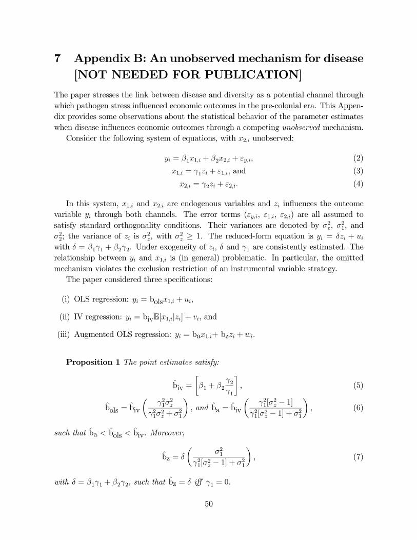
7 Appendix B: An unobserved mechanism for disease

[NOT NEEDED FOR PUBLICATION]

The paper stresses the link between disease and diversity as a potential channel through

which pathogen stress influenced economic outcomes in the pre-colonial era. This Appen-

dix provides some observations about the statistical behavior of the parameter estimates

when disease influences economic outcomes through a competing unobserved mechanism.

Consider the following system of equations, with 2 unobserved:

= 11 + 22 + , (2)

1 = 1 + 1, and (3)

2 = 2 + 2. (4)

In this system, 1 and 2 are endogenous variables and influences the outcome

variable through both channels. The error terms (, 1, 2) are all assumed to

satisfy standard orthogonality conditions. Their variances are denoted by 2, 21, and

22; the variance of is 2, with 2 ≥ 1. The reduced-form equation is = +

with = 11 + 22. Under exogeneity of , and 1 are consistently estimated. The

relationship between and 1 is (in general) problematic. In particular, the omitted

mechanism violates the exclusion restriction of an instrumental variable strategy.

The paper considered three specifications:

(i) OLS regression: = bols1 + ,

(ii) IV regression: = bivE[1|] + , and

(iii) Augmented OLS regression: = ba1+ bz + .

Proposition 1 The point estimates satisfy:

b̂iv =

∙1 + 2

21

¸, (5)

b̂ols = b̂iv

µ21

2

212 + 21

¶, and b̂a = b̂iv

µ21[

2 − 1]

21[2 − 1] + 21

¶, (6)

such that b̂a b̂ols b̂iv. Moreover,

b̂z =

µ21

21[2 − 1] + 21

¶, (7)

with = 11 + 22, such that b̂z = iff 1 = 0.

50

In the context of the paper, the previous econometric model suggests that the reduced-

form estimate is consistent but not informative about direct or indirect influences of

disease on development. The “first-stage” (3) for the effect of disease on diversity can

be consistently estimated. However, it is not possible to identify the (causal) effect of

diversity on economic outcomes unless one assumes that 2 = 0 (or that 2 = 0). Under

such exclusion restriction, b̂iv = 1. The problematic case is when 22 6= 0 = 1 since

b̂iv = 221, which is unrelated to the causal effect of diversity on development. It is

not possible to rule out this case as 2 is unobserved. One can rely on the correlation

between observables and ethnic diversity as a way to determine the correlation between

unobservables and diversity that would nulify the effect of diversity on development; see,

e.g., Bellows and Miguel ([10], Appendix A). This strategy requires the control variables

to be “representative,” which is difficult to assess.29

Table B1. Hypothesis testing for no effect of disease on diversity in system (2)-(4).

(1) (2) (3) (4) (5) (7)

P-value for test

H0: b̂a = b̂ols 0.021 0.011 0.037 0.016 0.015 0.093

H0: b̂z = 0.248 0.217 0.472 0.364 0.511 0.659

Note.— The specifications correspond to those of Table 9. For example, column (7) includes

the full set of controls and the African indicator.

Moreover, if one assumes that there is no effect of disease on ethnic diversity, i.e.,

1 = 0, the previous ordering should change: one should see b̂a = b̂ols and b̂iv →∞ (i.e.,

the instrument is weak), and b̂z = . These equality restrictions are tested in Table B1.

The tests show that the OLS and Augmented OLS estimates of diversity are statistically

different even once the African indicator is included (column (7)). These findings are

reassuring about the influence of disease on ethnic diversity. The reduced-form estimate

of disease , however, is indistinguishable from the Augmented OLS estimate.

Proof of Proposition 1. Since the statistical structure in (2)-(4) is rather sim-

ple, the behavior of the point estimates can be determined in closed-form. The OLS

regression yields estimates b̂ols = ( 1)(1), which can be written as b̂ols =

( 1)(1), or more compactly as

b̂ols = 1

µ()

(1)

¶= 1

µ2

212 + 21

¶.

29Regardless of the exclusion restriction, one should see b̂a b̂ols b̂iv. The empirical findings fromspecifications (i)-(iii) in Table 9 are consistent with the previous ordering.

51

This expression can be written in terms of primitives as

b̂ols = 1

µ21

2

212 + 21

¶+ 2

21

µ21

2

212 + 21

¶,

=

∙1 + 2

21

¸µ21

2

212 + 21

¶. (8)

The IV regression yields estimates ( ) = b̂iv(1 ) or more compactly as

( ) = b̂iv(1 ), which can be written in terms of primitives as

b̂iv =

∙1 + 2

21

¸. (9)

The augmented OLS regression yields

b̂a =b1 − bb11− b1b1

, and b̂z =b − b1b11− b1b1

,

where b is the slope of the regression of on ; see Johnston ([1], p. 81). For instance,

b1 = b̂ols, b = , b1 = 1,and b1 = 1(1), so that simple substitutions

yield

b̂a =b̂ols − b11− 1b1

=(1)b̂ols − 1(1)− 21

,

which can be further simplified as

b̂a = 1

µ[2 − 1]

21[2 − 1] + 21

¶.

In terms of primitives, the previous expresion is

b̂a = 1

µ21[

2 − 1]

21[2 − 1] + 21

¶+ 2

21

µ21[

2 − 1]

21[2 − 1] + 21

¶,

=

∙1 + 2

21

¸µ21[

2 − 1]

21[2 − 1] + 21

¶. (10)

Likewise, one can obtain

b̂z = − b̂ols11− 1b1

=

µ21

21[2 − 1] + 21

¶. (11)

Then, (8), (9), (10), and (11) imply that the point estimates of 1 on , and on

satisfy (6).

52

8 Appendix C: Robustness checks and supplemental

results for Tables 9, 10, and 11 [NOT NEEDED

FOR PUBLICATION]

Results complementing Table 9. Table C1 presents robustness checks for Table 9,

panel A. These results show that the negative OLS correlation between ethnic diversity

and large or impressive structures is robust to additional controls and sub-samples. The

estimates are based on non-agricultural societies only.

Table C1. Robustness checks for Table 9, panel A. OLS estimates.

Dependent variable: Large or impressive structures

(1) (2) (3) (4) (5) (7)

A. An alternative measure of ethnic diversity

Ethnic groups −0.034∗∗∗ −0.038∗∗∗ −0.025∗∗ −0.025∗∗ −0.023∗∗ −0.004within 250 m. (0.009) (0.009) (0.010) (0.010) (0.010) (0.010)

B. Using religious, military, or industrial structures only

Ethnic groups −0.002∗∗∗ −0.003∗∗∗ −0.002∗ −0.002∗∗ −0.002 0.002

within 500 m. (0.001) (0.001) (0.001) (0.001) (0.001) (0.001)

N. Obs. 119 118 114 114 114 114

C. Controlling for density instead of population size

Ethnic groups −0.014∗∗∗ −0.016∗∗∗ −0.011∗∗∗ −0.011∗∗∗ −0.011∗∗∗ −0.003within 500 m. (0.003) (0.004) (0.004) (0.004) (0.004) (0.007)

N. Obs. 119 117 113 113 113 113

D. Societies in sub-Saharan Africa and tropical America

Ethnic groups −0.009∗∗ −0.013∗∗∗ −0.015∗∗∗ −0.016∗∗∗ −0.015∗∗∗ −0.012∗within 500 m. (0.003) (0.003) (0.004) (0.004) (0.004) (0.007)

N. Obs. 52 52 50 50 50 50

E. Societies in sub-Saharan Africa and Eurasia

Ethnic groups −0.018∗∗∗ −0.019∗∗∗ −0.014∗∗∗ −0.014∗∗∗ −0.014∗∗∗ −0.005within 500 m. (0.003) (0.003) (0.004) (0.004) (0.004) (0.007)

N. Obs. 93 92 88 88 88 88

F. Excluding societies in sub-Saharan Africa

Ethnic groups 0.005 0.008 0.013 0.009 0.011 0.011

within 500 m. (0.011) (0.009) (0.010) (0.010) (0.011) (0.011)

N. Obs. 93 92 90 90 90 90

Note.— The specifications follow those of Table 2 and 6. In parentheses are robust standard

errors. ∗∗∗, ∗∗ and ∗ denote statistical significance at the 1, 5, and 10 percent level.

53

Results complementing Tables 10 and 11. Table C2 presents robustness checks

for Table 10, panel A. The table presents OLS correlations between pathogen stress and

current income per capita for alternative specifications, controls, and sub-samples.

Table C2. Robustness checks for Table 10, panel A. Pathogen stress and GDP per capita.

Dependent variable: log-GDP per capita

(1) (2) (3) (4) (5) (6)

A. Using the presence of pathogens only

Pathogen −0.409∗∗∗ −0.305∗∗∗ −0.267∗∗∗ −0.273∗∗∗ −0.259∗∗∗ −0.248∗∗∗presence (0.04) (0.05) (0.06) (0.06) (0.08) (0.08)

N. Obs. 67 66 66 65 65 65

B. Adding pre-colonial food surplus and tech. sophistication as controls

Pathogen −0.172∗∗∗ −0.155∗∗∗ −0.128∗∗∗ −0.131∗∗∗ −0.102∗∗ −0.06stress (0.03) (0.03) (0.03) (0.02) (0.04) (0.04)

N. Obs. 67 66 66 65 65 65

C. Including non-colonies

Pathogen −0.234∗∗∗ −0.233∗∗∗ −0.207∗∗∗ −0.190∗∗∗ −0.180∗∗∗ −0.104∗∗stress (0.02) (0.02) (0.02) (0.02) (0.02) (0.04)

N. Obs. 89 88 88 87 87 88

D. Excluding sub-Saharan Africa

Pathogen −0.197∗∗∗ −0.101∗∗ −0.082∗∗ −0.091∗∗ −0.018 −0.045stress (0.03) (0.03) (0.04) (0.04) (0.06) (0.09)

N. Obs. 40 39 39 39 39 39

E. Only Africa (sub-Saharan and North)

Pathogen −0.112∗∗ −0.111∗∗ −0.139∗∗∗ −0.141∗∗∗ −0.180∗∗ 0.06

stress (0.05) (0.05) (0.04) (0.05) (0.06) (0.11)

N. Obs. 32 32 32 31 31 31

F. Sub-Saharan Africa and South and Central America

Pathogen −0.191∗∗∗ −0.166∗∗∗ −0.101∗∗ −0.100∗∗ −0.107∗∗ −0.008stress (0.03) (0.03) (0.04) (0.03) (0.05) (0.06)

N. Obs. 51 51 51 50 50 50

Note.— In parentheses are robust standard errors. ∗∗∗, ∗∗ and ∗ denote statistical significanceat the 1, 5, and 10 percent level. Each specification corresponds to those of Table 10.

54

Table C3 presents robustness checks for Table 10, panel B. It shows that pathogen

stress helps predict current indices of ethnolinguistic fractionalization. The previous as-

sociation only weakens when all the environmental controls are in place or when Africa is

excluded from the sample.

Table C3. Robustness checks for Table 10, panel B. Pathogen stress and ELF.

Dependent variable: Ethnolinguistic fractionalization

(1) (2) (3) (4) (5) (6)

A. Using the presence of pathogens only

Pathogen 0.059∗∗∗ 0.061∗∗∗ 0.058∗∗∗ 0.063∗∗∗ 0.074∗∗ 0.017

presence (0.01) (0.02) (0.02) (0.02) (0.02) (0.03)

N. Obs. 71 68 68 68 68 68

B. Adding pre-colonial food surplus and tech. sophistication

Pathogen 0.033∗∗∗ 0.035∗∗∗ 0.028∗∗ 0.030∗∗ 0.033∗∗ −0.014stress (0.01) (0.01) (0.01) (0.01) (0.01) (0.01)

N. Obs. 71 68 68 68 68 68

C. Including non-colonies

Pathogen 0.043∗∗∗ 0.045∗∗∗ 0.043∗∗∗ 0.048∗∗∗ 0.053∗∗∗ −0.004stress (0.007) (0.007) (0.008) (0.009) (0.009) (0.016)

N. Obs. 87 84 84 84 84 84

D. Excluding sub-Saharan Africa

Pathogen 0.001 −0.006 −0.006 −0.032 0.005 −0.019stress (0.01) (0.01) (0.01) (0.01) (0.01) (0.04)

N. Obs. 44 41 41 41 41 41

E. Only Africa (sub-Saharan and North)

Pathogen 0.019 0.030∗∗ 0.035∗∗ 0.029 0.048∗∗ −0.049stress (0.01) (0.01) (0.01) (0.02) (0.02) (0.03)

N. Obs. 34 33 33 33 33 33

F. Sub-Saharan Africa and South and Central America

Pathogen 0.045∗∗∗ 0.047∗∗∗ 0.021 0.026∗ 0.023 −0.011stress (0.01) (0.01) (0.01) (0.02) (0.02) (0.02)

N. Obs. 53 52 52 52 52 52

Note.— In parentheses are robust standard errors. ∗∗∗, ∗∗ and ∗ denote statistical significanceat the 1, 5, and 10 percent level. Each specification corresponds to those of Table 10.

55

Table C4 presents robustness checks for Table 11, panel A, which pertain to the OLS

correlations between pre-colonial ethnic diversity and current income per capita.

Table C4. Robustness checks for Table 11, panel A. Ethnic diversity and GDP per capita.

Dependent variable: log-GDP per capita

(1) (2) (3) (4) (5) (6)

A. Adding food surplus and tech. sophistication as controls

Ethnic groups −0.014∗∗∗ −0.014∗∗∗ −0.012∗∗∗ −0.012∗∗ −0.008∗ −0.005in 500 m. (0.003) (0.003) (0.004) (0.005) (0.004) (0.004)

N. Obs. 67 66 66 65 66 66

B. Using an alternative measure of ethnic diversity

Ethnic groups −0.056∗∗∗ −0.038∗∗∗ −0.026∗∗ −0.027∗∗ −0.016 −0.010in 250 m. (0.01) (0.01) (0.01) (0.01) (0.01) (0.01)

N. Obs. 67 66 66 65 66 66

C. Including non-colonies

Ethnic groups −0.023∗∗∗ −0.023∗∗∗ −0.019∗∗∗ −0.020∗∗∗ −0.016∗∗∗ −0.008∗in 500 m. (0.003) (0.003) (0.004) (0.005) (0.005) (0.005)

N. Obs. 87 86 86 85 85 86

D. Excluding sub-Saharan Africa

Ethnic groups −0.015 −0.005 −0.010 −0.015 −0.016 0.007

in 500 m. (0.01) (0.01) (0.01) (0.01) (0.01) (0.01)

N. Obs. 40 39 39 39 39 39

E. Only Africa (sub-Saharan and North)

Ethnic groups −0.009∗∗ −0.008∗∗ −0.008∗ −0.008 −0.006 0.015

in 500 m. (0.004) (0.004) (0.004) (0.007) (0.005) (0.007)

N. Obs. 32 32 32 31 32 32

F. Sub-Saharan Africa and South and Central America

Ethnic groups −0.017∗∗∗ −0.014∗∗∗ −0.007 −0.006 −0.005 0.002

in 500 m. (0.003) (0.003) (0.005) (0.005) (0.005) (0.005)

N. Obs. 51 51 51 50 51 51

Note.— In parentheses are robust standard errors. ∗∗∗, ∗∗ and ∗ denote statistical significanceat the 1, 5, and 10 percent level. Each specification corresponds to those of Table 11.

56

Table C5 presents IV estimates of pre-colonial ethnic diversity and current income per

capita, using pathogen stress as instrument for ethnic diversity. This strategy is likely

biased becuase the exclusion restriction is difficult to accept. Yet, as noted in the text, the

IV strategy serves as a complementary strategy relative to the baseline OLS correlations.

Table C5. Pre-colonial ethnic diversity and current income (IV, second-stage).

Dependent variable: log-GDP per capita

(1) (2) (3) (4) (5) (6)

A. Using the presence of pathogens only

Ethnic groups −0.045∗∗∗ −0.033∗∗∗ −0.034∗∗∗ −0.035∗∗∗ −0.030∗∗ −0.038in 500 m. (0.012) (0.009) (0.012) (0.012) (0.013) (0.024)

N. Obs. 67 66 66 65 66 66

B. Adding food surplus and tech. sophistication as controls

Ethnic groups −0.033∗∗∗ −0.029∗∗∗ −0.029∗∗∗ −0.030∗∗∗ −0.023∗∗ −0.022in 500 m. (0.009) (0.008) (0.009) (0.010) (0.012) (0.014)

N. Obs. 67 66 66 65 66 66

C. Using an alternative measure of ethnic diversity

Ethnic groups −0.150∗∗∗ −0.111∗∗∗ −0.097∗∗∗ −0.107∗∗ −0.071∗∗ −0.083∗in 250 m. (0.040) (0.032) (0.036) (0.040) (0.033) (0.047)

N. Obs. 67 66 66 65 66 66

D. Including non-colonies

Ethnic groups −0.047∗∗∗ −0.046∗∗∗ −0.046∗∗∗ −0.038∗∗∗ −0.042∗∗∗ −0.035∗in 500 m. (0.009) (0.008) (0.010) (0.007) (0.010) (0.018)

N. Obs. 87 86 86 85 85 86

E. Excluding sub-Saharan Africa

Ethnic groups −0.290 −0.225 −0.116 −0.118 −0.035 −0.130in 500 m. (0.403) (0.431) (0.152) (0.115) (0.060) (0.411)

N. Obs. 40 39 39 39 39 39

F. Only Africa (sub-Saharan and North)

Ethnic groups −0.018∗∗ −0.017∗∗ −0.022∗∗ −0.037∗∗ −0.024∗∗ −0.141in 500 m. (0.008) (0.008) (0.008) (0.013) (0.011) (0.686)

N. Obs. 32 32 32 31 32 32

F. Sub-Saharan Africa and South and Central America

Ethnic groups −0.030∗∗∗ −0.028∗∗∗ −0.022∗∗ −0.024∗∗ −0.018∗∗ −0.007in 500 m. (0.006) (0.007) (0.009) (0.010) (0.009) (0.048)

N. Obs. 51 51 51 50 51 51

Note.— In parentheses are robust standard errors. ∗∗∗, ∗∗ and ∗ denote statistical significanceat the 1, 5, and 10 percent level. Each specification corresponds to those of Table 8.

57

9 Appendix D: Country codes for the SCCS [NOT

NEEDED FOR PUBLICATION]

The following list reports the countries where each of the 186 societies in the SCCS is

present:

1 = ZAF,NAM,BWA, 2 = NAM,BWA,AGO, 3 = MOZ,ZAF, 4 = ZMB, NAM,

AGO,BWA, 5 = AGO,6 = CGO,AGO, 7 = ZMB, 8 = TZA,MWI, 9 = TZA, 10 = TZA,

11 = KEN, 12 = UGA, 13 = CGO, 14 = CGO, 15 = CMR, 16 = NGA,CMR, 17 = NGA,

18 = BEN,NGA, 19 = GHA, 20 = SLE, 21 = SEN,GMB,MRT, 22 = MLI,BFA,SEN, 23

= GHA, 24 = MLI, 25 = NER,NGA,CMR,26 = NGA,NER,SDN,CMR,GHA,CIV,TCD,

27 = TCD,CMR, 28 = ZAR,SDN,CAF, 29 = SDN, 30 = SDN, 31 = SDN, 32 = ETH, 33

= ETH, 34 = KEN,TZA, 35 = ETH, 36 = SOM,ETH,YEM,KEN,DJI, 37 = ETH, 38 =

ERI, 39 = SDN,EGY, 40 = TCD,LBY,NER,NGA, 41 = NER,MLI,DZA,BFA,LBY, 42 =

MAR, 43 = EGY, 44 = ISR, 45 = IRQ, 46 = SAU, 47 = TUR, 48 = ALB, 49 = ITA, 50 =

ESP,FRA, 51 = IRL, 52 = NOR,SWE,FIN, 53 = RUS, 54 = RUS, 55 = TUR,RUS, 56 =

ARM,RUS, 57 = TUR,IRN,IRQ, SYR, 58 = IRN, 59 = PAK,IND, 60 = IND, 61 = IND,

62 = IND,BGD, 63 = IND,NPL, 64 = PAK, 65 = KAZ,UZB,CHN,MNG, 66 = MNG, 67

= CHN,VNM,THA, 68 = IND,NPL,BTN, 69 = IND,BGD, 70 = IND,BUR, 71 = BUR,

72 = LAO, 73 = VNM, 74 = VNM, 75 = KHM, 76 = THA, 77 = BUR,MYS,SGP,THA,

78 = IND, 79 = IND, 80 = LKA, 81 = MDG, 82 = MYS, 83 = IDN, 84 = IDN, 85 =

MYS, 86 = MYS,PHL, 87 = IDN, 88 = IDN, 89 = IDN, 90 = AUS, 91 = AUS, 92 =

PNG, 93 = IDN, 94 = IDN, 95 = PNG, 96 = PNG, 97 = PNG, 98 = PNG, 99 = PNG,

100 = SLB, 101 = VUT, 102 = FJI,NZL 103 = PYF, 104 = NZL,AUS, 105 = PYF, 106

= WSM, 107 = KIR, 108 = MHL, 109 = FSM, 110 = FSM, 111 = PLW, 112 = PHL,

113 = CHN, 114 = CHN, 115 = CHN, 116 = KOR, 117 = JPN, 118 = JPN,RUS, 119

= RUS, 120 = RUS, 121 = RUS, 122 = USA, 123 = USA, 124 = CAN, 125 = CAN,

126 = CAN,USA, 127 = CAN, 128 = CAN, 129 = CAN, 130 = USA, 131 = CAN,USA,

132 = CAN, 133 = USA, 134 = USA, 135 = USA, 136 = USA, 137 = USA, 138 = USA,

139 = CAN,USA, 140 = USA, 141 = USA, 142 = USA, 143 = USA, 144 = CAN,USA,

145 = USA, 146 = USA, 147 = USA, 148 = USA,MEX, 149 = USA, 150 = USA, 151 =

USA,MEX, 152 = MEX, 153 = MEX, 154 = MEX, 155 = GTM, 156 = HND,NIC, 157 =

CRI, 158 = PAN,COL, 159 = COL,VEN, 160 = HTI, 161 = DMA, 162 = VEN,GUY, 163

= VEN,BRA, 164 = GUY, 165 = SUR, 166 = BRA, 167 = BRA,COL, 168 = ECU,COL,

169 = ECU,PER, 170 = PER,BRA, 171 = PER, 172 = BOL,PER,CHI, 173 = BOL, 174

= BRA, 175 = BRA, 176 = BRA, 177 = BRA, 178 = BRA, 179 = BRA, 180 = BRA, 181

= PRY,URY,BRA, 182 = PRY, 183 = ARG, 184 = CHL, 185 = ARG, 186 = ARG,CHL.

58

References

[1] Johnston, J. (1984) Econometric Methods, McGraw Hill.

59