diseño aerogenerador1

Local design, testing and manufacturing of small mixedairfoil wind turbine blades of glass ®ber reinforced plastics

Part I: Design of the blade and root

S.M. Habalia,*, I.A. Salehb

aMechanical Engineering Department, Faculty of Engineering and Technology, University of Jordan, Amman, JordanbRenewable Energy Center, Royal Scienti®c Society, Amman, Jordan

Received 27 October 1998; accepted 16 May 1999

Abstract

Wind energy has attracted a great deal of attention in recent years in Jordan as one of the possiblealternative renewable energy resources. Almost of the local research and development activities in this®eld were directed to explore, develop, and optimal utilization of energy systems. The time has come toestablish a link between local scienti®c (academic) work and local industries to produce a usabletechnology which will increase the local share in an inevitably emerging wind energy industry in Jordan.To achieve this goal, a well founded manufacturing base is required. The most important component ofa Wind Energy Converter is the rotor. The e�ciency of a rotor is characterized by its pro®le (airfoilsection) and the corresponding aerodynamic design. A selection procedure of airfoil section and theaerodynamic design of the blade for a small wind turbine are discussed and implemented in this paper(Part I). It is found that for small blades up to 5 m long, two di�erent air foils mixed at the outer thirdof the span will be su�cient and demonstrated good strength and aerodynamic characteristics. As acomposite material, the Glass Fiber Reinforced Plastic was used in designing the rotor blade. This rotorwas then installed on 15 kW grid-connected-pitch-controlled machine. A static proof load test indicatedthat this blade could withstand loads ten times the normal working thrust, and a ®eld performance testshowed that the rotor blade has a 41.2% measured average power coe�cient. # 1999 Elsevier ScienceLtd. All rights reserved.

Keywords: Mixed airfoil blades of CM; Mixed airfoil blades of GRP; Mixed airfoil blades rotor of GRP; Design ofmixed airfoil-blades rotor of GRP

Energy Conversion & Management 41 (2000) 249±280

0196-8904/00/$ - see front matter # 1999 Elsevier Science Ltd. All rights reserved.PII: S0196-8904(99)00103-X

www.elsevier.com/locate/enconman

* Corresponding author.E-mail address: [email protected] (S.M. Habali)

Abbreviations: CM, Composite Materials; GRP, Glass Fiber Reinforced Plastics.

Nomenclature

Az Blade-cross sectional area perpendicular to z axis (blade axis)a Axial interface factora ' Tangential interface factorB Number of bladesL Lift forceD Drag forceCD Drug coe�cientCL Lift coe�cientCm Moment coe�cientCx Force coe�cient in x directionCy Force coe�cient in y direction.c Chord lengthd Diameterdi Inside diameterdo Outside diameterE Modulus of elasticityF Circulation reduction factorG Circulation of one blade at radius rG1 Circulation of rotor with in®nite number of bladesFc Centrifugal forceFx Force component in x directionFy Force component in y directionFz Force component in z directionFt Tangential forcemx Bending moment about x axismy Bending moment about y axisf Tip losses factor, Line frequencyG Shear modulusIx Area moment of inertia around x axis.Iy Area moment of inertia around y axisIz Area moment of inertia around the z axis (polar moment of inertia)m Time rate of change of air massP PowerCp Power coe�cientp Ambient pressureQ TorqueR Total radiusr Local radiusT Thrust forceU Local wind velocity

S.M. Habali, I.A. Saleh / Energy Conversion & Management 41 (2000) 249±280250

1. Introduction

In order for a wind energy industry to be established in Jordan, a founded manufacturingbase is required. Jordan has virtually hundreds of di�erent kinds of industries, but no one isspecialized in manufacturing wind system components. Thus, a problem exists which will beaddressed in this paper to establish a local manufacturing procedure and capability for GlassFiber Reinforced Plastic (GRP) wind turbine blades and to identify the basic components ofthis technology which are required from the local market.Wind turbine blades must be designed to operate in the most unpredictably severe

environmental conditions and still give satisfactory performances for the lifetime of the system.Rotor blade design relies heavily on aerodynamic theory, since the blade is an aerodynamicbody having special geometry characterized mainly by an airfoil cross section. Extensivecalculations will be necessary in order to determine the blade parameters, such as chord,thickness and twist distributions and taper, that are matched with the selected airfoil section. Abrief summary of rotor blade design is, therefore, given to de®ne the various parametersgoverning blade design and with the help of a special software, a complete aerodynamicanalysis was performed. A three-dimensional (3D) solid model is then created and a FEManalysis was performed using a powerful computer which yielded a simulation to the actualblade operating under loads. A ®nal blade was veri®ed and a full scale model was made.

V Wind speed velocitya Angle of attackat Angle of attack of blade tipb Twist angle of bladeZ E�ciencyl Tip speed ratio of rotor bladeF Flow angle of relative wind speed to the airfoilFt Flow angle of relative wind speed to the airfoil tipO Angular speed of rotoro Angular speed of waker Density of airs Magnitude of stresse Magnitude of strainLb Length of bladeFEM Finite Element Methodrcm Blade center of mass measured from the rootGRP Glass Fiber Reinforced Plastic3D Three dimensionalSERI Solar Energy Research Institute.NACANational Advisory Committee of Aeronautics.WEC Wind Energy Converter

S.M. Habali, I.A. Saleh / Energy Conversion & Management 41 (2000) 249±280 251

For practical purposes, more than one airfoil section must be chosen to ®t the thicknessdistribution where, closer to the root, a thick section is needed for structural reasons, and thinnersections are used along the outboard region with a smooth transition from root to tip. One of theobjectives of this research work is to develop the basic engineering design of GRP blades and alsoto establish the procedure for the local manufacturing. Ultimately, this work will contributetoward the initiation of a GRP blade test facility which can lead to establishing a local design code.Much computer software has been written to simulate what happens in reality during the rotor

blade ¯ight and to attempt to predict the resulting aerodynamic loads and their variations. Forexample, Harten [1] used a software package called loads that analyzes blade loads for rigidrotors of simple geometry for the Grumman WS33 wind turbine and calculated that thesensitivity of the load predictions to the phase of the turbulent wind simulation record stressedthe need for improving wind simulation techniques. The blades are designed and constructed towithstand loads resulting from normal operation, gusts, or turbulence, which induce majoralternating stresses, and therefore, the material used (GRP) must be capable of resisting thefatigue resulting from them. In this context, a variety of blade designs were suggested by Park [2],but more advanced blades having optimized geometry were introduced by Jackson et al. [3]. Ingeneral, the design of a wind turbine rotor consists of two steps, as given by Lysen [4]:

1. the choice of basic parameters: type of airfoil, tip speed ratio and2. calculations of the setting angles and chord length at di�erent positions along the blade.

One of the most recent developments in blade design, which was consulted during this study, isthe special purpose thin airfoil family introduced by Tangler et al. [5] through the solar energyresearch institute (SERI), Golden, Colorado. These SERI blades were described by Davidson[6] as `the blades of the future' and could produce 31% more power than the traditionalDanish made blades. Most modern blades, however, have pro®les of the NACA 63nnn series.These pro®les have shown excellent properties for wind turbine blades, but some improvementscan still be achieved in the pro®les in the inner portion of the blades in order to make thepro®le su�ciently thick while still having high lifting force. For this reason, developments areproceeding to design thick airfoils for the in board region of rotor blades. An example of thisis the SERI S897 pro®le. Other examples are: the LS(1)-0421 and the NACA 63-621 pro®les. Itis interesting to notice the big di�erence among these pro®les; however all are suited for use.During the course of this work, one Jordanian company was identi®ed and has succeeded in

adapting to this new technology and, according to the procedure set forth, had produced ahigh quality 5 m GRP blade. The blade has also passed successfully the pre-assigned stress testand, when installed on a functional wind turbine, performed satisfactorily with a favorablepower coe�cient of 41.2%.

2. Design of the rotor blade

2.1. Blade size and material

The philosophy underlying the choice of the blade size was that a small blade will be toosti� by nature and unable to exhibit the behavior of full size blades used for electricity


generation. On the other hand, a large blade will exceed the capabilities of the technical and®nancial resources. Hence, the decision was made to experiment with a 5 m long blade whichhas the characteristics of large blades and the handling convenience of small blades.The choice of the material based on some considerations, such as the material weight and

strength besides it's availability in Jordan, so that it can be adapted to mass production. Thischoice of the GRP can be related to many attributes, one of which is the availability of thepolyester resin which is locally produced.

2.2. Blade shape and pro®le

2.2.1. Aerodynamic theory

2.2.1.1. Overview of rotor blade aerodynamics. Rotor blade design relies heavily on aerodynamictheory. The blade is an aerodynamic body having a special geometry mainly characterized byan airfoil cross section. Extensive calculations are necessary to determine the blade parameters,such as chord, thickness and twist distributions over the blade length and taper that arematched with the selected airfoil sections. For practical purposes, more than one airfoil sectionmust be chosen to ®t the thickness distribution, where the thickness decreases with the radiusof the rotor (blade length) and a smooth transition condition is satis®ed.The ¯ight of a rotor blade is a complex phenomenon which can not be modeled exactly.

This complexity arises from the fact that the ¯ow of the air around the blade is 3D withvarious vortex sheddings, resulting from the variable rotational speed. This is also coupled withthe variation of wind speed distribution along the blade caused by the wind shear and the largescale boundary layer on the earth surface. This phenomenon, however, can be approximatelydescribed by imposing several assumptions. One of the simplest descriptions of extractingenergy from the wind is the one dimensional, incompressible, non-viscous ¯ow model using theaxial momentum theory, including the rotational wake e�ects. More recently, Wilson andLissaman [7] have analyzed the aerodynamic performance of wind turbines.The momentum theory cannot provide the necessary information on how to design the rotor

blades. However, the momentum theory when combined with the blade element theory willthen yield this kind of information.

2.2.1.2. The axial momentum theory. Three principal assumptions are made:

. the ¯ow is completely axial,

. the ¯ow is rotationally symmetric, and

. no friction occurs when the air passes the wind turbine rotor.

From Fig. 1 we obtain:

. the continuity equation:

UA � U1A1 �1�. momentum (thrust) equation:

T � _m�VÿU1� � rAU�VÿU1� �2�


. Bernoulli upwind

p0 � 0:5rV 2 � p� 0:5rU 2 �3�. Bernoulli downwind

p0 � 0:5rU 21 � p 0 � 0:5rU 2 �4�

Thus,

Dp � pÿ p 0 � 0:5rÿV 2 ÿU 2

1

� �5�Combining Eqs. (2) and (5) with

T � ADp �6�yields

U � 0:5�V�U1� �7�The power extracted will then be:

P � 0:5 _mÿV 2 ÿU 2

1

� � 0:5rUAÿV 2 ÿU 2

1

� �8�Now, denoting a power coe�cient by

Cp � P

0:5rV 3A�9�

and knowing that the ¯ow has been retarded at the rotor disc by slowing down a certainamount a, then we get:

U � �1ÿ a�V �10�Eqs. (7) and (10) give

Fig. 1. Axial ¯ow model.


U1 � �1ÿ 2a�V �11�Substituting Eqs. (10) and (11) into Eq. (8) and the result into Eq. (9) gives the powercoe�cient of

Cp � 4a�1ÿ a�2 �12�which has a maximum when a � 1=3, as shown in Fig. 2.In order to enhance the results and make them close to reality, the e�ect of wake rotation

will be included. In describing this e�ect, the assumption is made that upstream of the rotor,the ¯ow is entirely axial and that the ¯ow downstream rotates with an angular velocity o , butremains irrotational.Expressions for torque and power may be obtained by considering the ¯ow through an

annulus at radius r with area

dA � 2pr dr �13�By changing the momentum in the air in the tangential direction, tangential forces Ft act uponthe rotor as:

dFt � _m dV � rU dAor �14�Substitute Eq. (13) into Eq. (14) we obtain

dFt � 2prUor2 dr �15�The torque generated in the annulus dr is:

dQ � 2prUor3 dr �16�and since

P � Qo �17�the power extracted is

Fig. 2. Power coe�cient Ð axial interference factor curve.


dP � 2prOUor3 dr �18�The total torque and the power of the rotor become

Q � 2pr�Uor3 dr �19�

and

P � 2prO�Uor3 dr �20�

In order to be able to calculate torque and power, one must have the values of the wake'sangular velocities o by introducing the tangential induction factor a ' [6] as:

a 0 � 0:5oO

�21�

2.2.1.3. Blade element theory. Two main assumptions govern this theory:

. The forces and the moments acting on a blade element are solely due to the lift and dragcharacteristics of the pro®le section of that blade element.

. There should be no interference between adjacent blade elements because the forces on eachelement are calculated with their local wind velocities. The ¯ow around the blade element (oflength dr ) at radius r may be considered as a two-dimensional ¯ow as shown in Fig. 3. Inthis representation, the angular velocity O of the rotor is assumed to have the value of the®nal rotational velocity o in the wake, [4], which is an approximation to Eq. (21) by settinga 0 � 1.

Fig. 3. Velocity and forces at a blade element at radius r.


De®ning

dq � 0:5rW 2 dA � 0:5rW 2c dr �22�gives:

CL � dL

dq�23�

CD � dD

dq�24�

Cx � dFx

dq�25�

and

Cy � dFy

dq�26�

The following trigonometric relations may be obtained from Fig. 3:

a � Fÿ b �27�

tan F � �1ÿ a�V�1� a 0 �Or �28�

Cy � CLcos F� CDsin F �29�

Cx � CLsin Fÿ CDcos F �30�Expressions for the thrust, dT, and the torque, dQ, for an element dr at radius r can now bederived as follows:

dT � BCy dq � BCy0:5rW 2c dr �31�and

dQ � BCx dqr � BCx0:5rW 2cr dr �32�where B is the number of blades.The thrust and torque equations were also derived using the axial moment theory, but with

the assumption that no friction occurs. Hence, in order to equate the two results, we mustassume CD � 0, then equating Eq. (2) to Eqs. (31) and (16) to Eq. (32) gives:

a

1ÿ a� cBCy

8prsin2F�33�


and

a 0

1� a 0� cBCx

8prsin Fcos F�34�

From Fig. 3 we can conclude that:

W � U

sin F� V�1ÿ a�

sin F�35�

or

W � Or�1� a 0 �cos F

�36�

The local solidity ratio of the rotor is de®ned as:

s � cB

2pr�37�

Solving Eqs. (33) and (34) for a and a ', respectively, gives:

a � 1ÿ4sin2F=sCy

�� 1�38�

and

a 0 � 1

�4sin Fcos F=sCx� ÿ 1�39�

With a ®nite number of blades (e.g. B � 3), the assumption that the ¯ow through the rotor isrotationally symmetric obviously does not hold, in addition to the dimensional ¯owassumption. The e�ects due to the ®nite number of blades results in the performance lossesconcentrated near the tip of the blade. This phenomenon, known as the tip losses model, was®rst analyzed by Prandtl [8]. The tip losses are expressed by a circulation reduction factorde®ned by:

F � BGG1� 2

parcos�eÿf� �40�

where G is the actual circulation of one blade at radius r, and G1 is the circulation of a rotorwith an in®nite number of blades as was calculated in the axial momentum theory, and

f � �B=2��Rÿ r�rsin F

�41�

Prandtl [13] gives, as a result, the modi®ed axial and tangential velocity factors:

a � 1

�4sin2F�F=ÿsCy

�� 1�42�


and

a 0 � 1

�4sin Fcos F�F=�sCx� ÿ 1�43�

Note that the Prandtl factor F does not change the relation between the two factors aspreviously derived.

3. Airfoil selection

Airfoils chosen for wind turbine applications have focused on the half century old NACA23nnn and NACA 44nn airfoil series. The NACA 23nnn series were found by Tangler [5], toexperience a large drop in maximum lift coe�cient, CL,max, as the airfoil becomes solid (dirty).This problem was also found on the NACA 44nnn series, however to a lesser extent.In an e�ort to solve this blade soiling problem, manufacturers began using the LS-1 and

NACA 63nnn series of airfoils. Both of these airfoil sections have their camber further backwhich provides some improvement in reducing the airfoil's CL,max sensitivity to roughnesse�ects. In addition, the NACA 63nnn provided a lower CL,max which helped control peakpower. However, this characteristic is desirable only over the tip region of the blade, and whenused on the inboard region, a degradation in energy production is expected. The LS-1 serieshave the opposite problem. This airfoil provides a desirable high CL,max toward the blade rootbut contributes to excessive peak power when used over the outboard portion of the blade.The excessive peak power must then be controlled, with undesirable reduction in blade solidityor a less e�cient blade operating pitch angle. Fig. 4a shows the two airfoil pro®les: LS(1)-0421and NACA 63-621.The FX-S airfoil family has in it's series the characteristics required for the outboard region

and also the tip. This family has a stable lift coe�cient (CL) at high angles of attack (low windspeed). In addition, their moment coe�cient, Cm, is smooth and almost constant over thewhole range of operating angles of attack [9]. The airfoil FX66-S-196, shown in Fig. 4b, will beselected for the outboard region of our blade.The inboard region of the blade must be thicker and have more material to withstand the

higher stresses and also have a smoother geometry transition to the circular connecting ¯angeat the root. The NACA 63-621 pro®le, shown in Fig. 4a, is selected for the inboard regionwhich has these characteristics and is very similar to the FX 66- S-196 pro®le. In addition, thepro®le similarities will simplify the transition from the inner to outer board regions.

4. Determination of the blade data

The design and construction of sophisticated wind turbine blades requires enormousamounts of data. Most important are those describing the geometry and structuralcharacteristics of the blade, such as length (radius of the rotor), thickness distribution, chordlength distribution, twist, root connection, etc.


4.1. Radius of the rotor

The radius of the rotor, i.e. the length of the rotor's blade, can be determined from therotor's area which depends in it's value on the rated power of the wind turbine. The ratedpower can be calculated from the equation

Prat � 0:5rV 3ratACp,rat �44�

The ®rst step is to identify the output capacity of the proposed wind turbine. This is an opendecision that depends on the needs and desires of the investor who wants to build the windmachine. The rated power, Prat, could range from a few hundred Watts to the order ofMegawatts.In our case, the rated power is taken at 20 kW. The rated power is only de®ned for pitch

controlled machines at one value of wind speed and power coe�cient. These two values can bechosen by experience and will directly in¯uence the size of the wind turbine rotor, i.e. thediameter. There are some theoretical bases for choosing the rated wind speed for a given windturbine [10]. However, experience has shown that most machines have a rated speed around 10m/s (Vrat � 10 m/s) and for small fast running machines lower values can be realized. Hence,for this design, Vrat � 9:5 m/s is selected.The maximum power coe�cient attained for an ideal wind turbine is Cp,max � 16=27 � 59%,

as was previously shown in Fig. 2. Also, from manufacturer data and test results of Ta'ani etal. [11], most machines of this size operate at Cp � 0:4�� 40%�, which is chosen for this design.Furthermore, for this design, the air density is selected as r � 1:25 kg/m3.

Fig. 4. Pro®les acceptable for use by mixed wind turbine blades: (a) on inboard region of the blade, and (b) on

outboard region of blade.


With the previous parameters selection, the only remaining unknown is the rotor's area thatcan be calculated from Eq. (44) as:A � Prat=�0:5rV 3

ratCp,rat� � 20000=�0:5� 1:25�9:5�30:4� � 93:3m2, and the diameter of the rotor will be d � �4A=p�0:5 � 10:9 m.

4.2. Dimensions of rotor

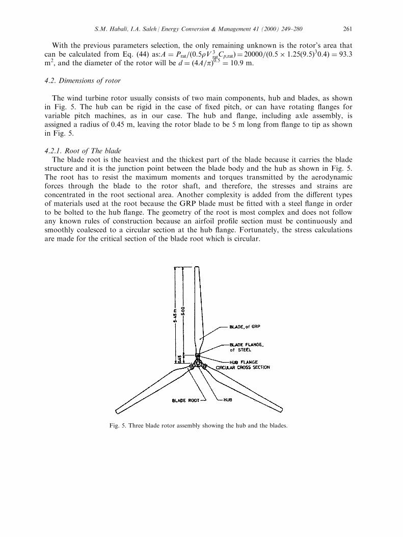
The wind turbine rotor usually consists of two main components, hub and blades, as shownin Fig. 5. The hub can be rigid in the case of ®xed pitch, or can have rotating ¯anges forvariable pitch machines, as in our case. The hub and ¯ange, including axle assembly, isassigned a radius of 0.45 m, leaving the rotor blade to be 5 m long from ¯ange to tip as shownin Fig. 5.

4.2.1. Root of The bladeThe blade root is the heaviest and the thickest part of the blade because it carries the blade

structure and it is the junction point between the blade body and the hub as shown in Fig. 5.The root has to resist the maximum moments and torques transmitted by the aerodynamicforces through the blade to the rotor shaft, and therefore, the stresses and strains areconcentrated in the root sectional area. Another complexity is added from the di�erent typesof materials used at the root because the GRP blade must be ®tted with a steel ¯ange in orderto be bolted to the hub ¯ange. The geometry of the root is most complex and does not followany known rules of construction because an airfoil pro®le section must be continuously andsmoothly coalesced to a circular section at the hub ¯ange. Fortunately, the stress calculationsare made for the critical section of the blade root which is circular.

Fig. 5. Three blade rotor assembly showing the hub and the blades.


4.3. Loading conditions

There are no special o�cial design rules for wind turbine blades based on speci®ed loading[12]. The evaluation of the ultimate strength and fatigue characteristics of rotor blade is basedon a static proof test [12]. The static proof load is derived from the assumption of an extremethrust load of trot � 300 N/m2 over the swept area. The total load acting on the rotor is then

Trot � trotArot �ÿ300 N=m2

��93:3 m2� � 27990 N

This load is equally shared among the three blades and distributed in a triangular pattern fromzero at the root center to the maximum value at the tip. This means that each blade of ourthree bladed rotor should withstand an extreme load of

Tblade � Trot=B � 27990 N=3 � 9330 N � 9:33 kN=blade

The blade should withstand this load without sustaining any damage.On fatigue, the certi®cation criterion states that at a load factor of 0:5�150� Arot=B�, [12],

the measured strain for GRP must be less than 0.2% in the side of the blade undercompression and less than 0.3% in the side of the blade under tension. Therefore, we have twoload cases:

Case 1: trot � 300 N/m2, Load 1 = (300 N/m2) (93.3 m2)/3 = 9.33 kN/bladeCase 2: trot � 150 N/m2, Load 2 � 150 N/m2 � 93.3 m2/3 = 4.665 kN/blade

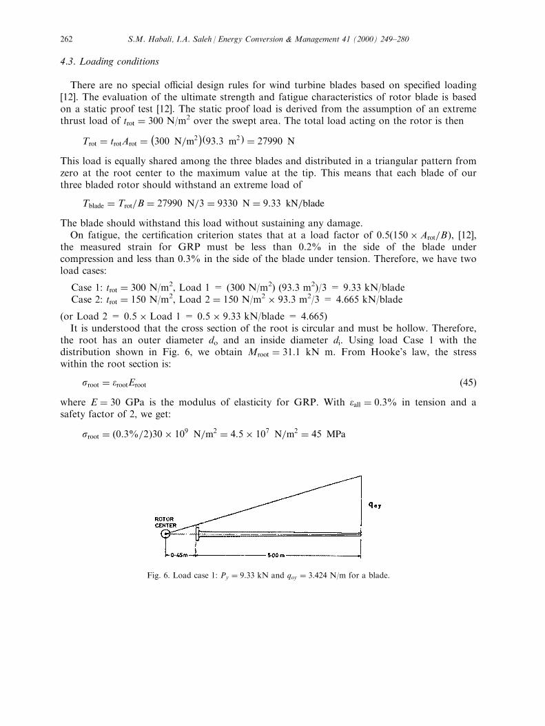
(or Load 2 = 0.5 � Load 1 = 0.5 � 9.33 kN/blade = 4.665)It is understood that the cross section of the root is circular and must be hollow. Therefore,

the root has an outer diameter do and an inside diameter di. Using load Case 1 with thedistribution shown in Fig. 6, we obtain Mroot � 31:1 kN m. From Hooke's law, the stresswithin the root section is:

sroot � erootEroot �45�where E � 30 GPa is the modulus of elasticity for GRP. With eall � 0:3% in tension and asafety factor of 2, we get:

sroot � �0:3%=2�30� 109 N=m2 � 4:5� 107 N=m2 � 45 MPa

Fig. 6. Load case 1: Py � 9:33 kN and qoy � 3:424 N/m for a blade.


Also, from the ¯exure formula, we have:

sroot � Mroot � rroot

Iroot

�46�

With: Iroot � p�d 4o ÿ d 4

i � and rroot � do

2 , Eq. (46) becomes

sroot � 32Mrootdo

2pÿd 4

o ÿ d 4i

� �47�

or

4:5� 107 N=m2 � �158:32� 103 Nm�doÿd 4

o ÿ d 4i

� �48�

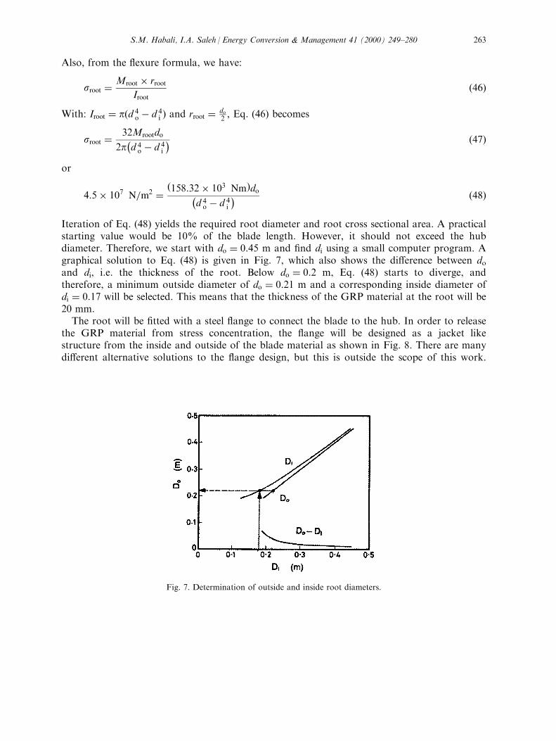
Iteration of Eq. (48) yields the required root diameter and root cross sectional area. A practicalstarting value would be 10% of the blade length. However, it should not exceed the hubdiameter. Therefore, we start with do � 0:45 m and ®nd di using a small computer program. Agraphical solution to Eq. (48) is given in Fig. 7, which also shows the di�erence between doand di, i.e. the thickness of the root. Below do � 0:2 m, Eq. (48) starts to diverge, andtherefore, a minimum outside diameter of do � 0:21 m and a corresponding inside diameter ofdi � 0:17 will be selected. This means that the thickness of the GRP material at the root will be20 mm.The root will be ®tted with a steel ¯ange to connect the blade to the hub. In order to release

the GRP material from stress concentration, the ¯ange will be designed as a jacket likestructure from the inside and outside of the blade material as shown in Fig. 8. There are manydi�erent alternative solutions to the ¯ange design, but this is outside the scope of this work.

Fig. 7. Determination of outside and inside root diameters.


The important criteria are avoiding sudden changes in geometry and keeping the glass ®berscontinuous from root to tip.

4.3.1. Blade taper (¯apwise)The blade geometry has two di�erent views, the ¯apwise view and the edgewise view as can

be seen from Fig. 9.A ¯apwise view of the proposed blade in Fig. 9a de®nes the chord length distribution of the

selected airfoil over the blade length and also shows the root region and the working region ofthe blade. The working region is the portion of the blade which has the actual airfoil section,

Fig. 8. Design of the blade root.

Fig. 9. Viewing the rotor blade geometry: (a) Flap-wise, and (b) Edge-wise.


and the root region is the portion which compensates the geometry between the airfoil pro®leand the completely circular section at the hub ¯ange and, therefore, does not contribute topower generation. The chord taper of the working region is also chosen linear to simplifymanufacturing.For a streamlined body with the dimensions already calculated and de®ned for the length,

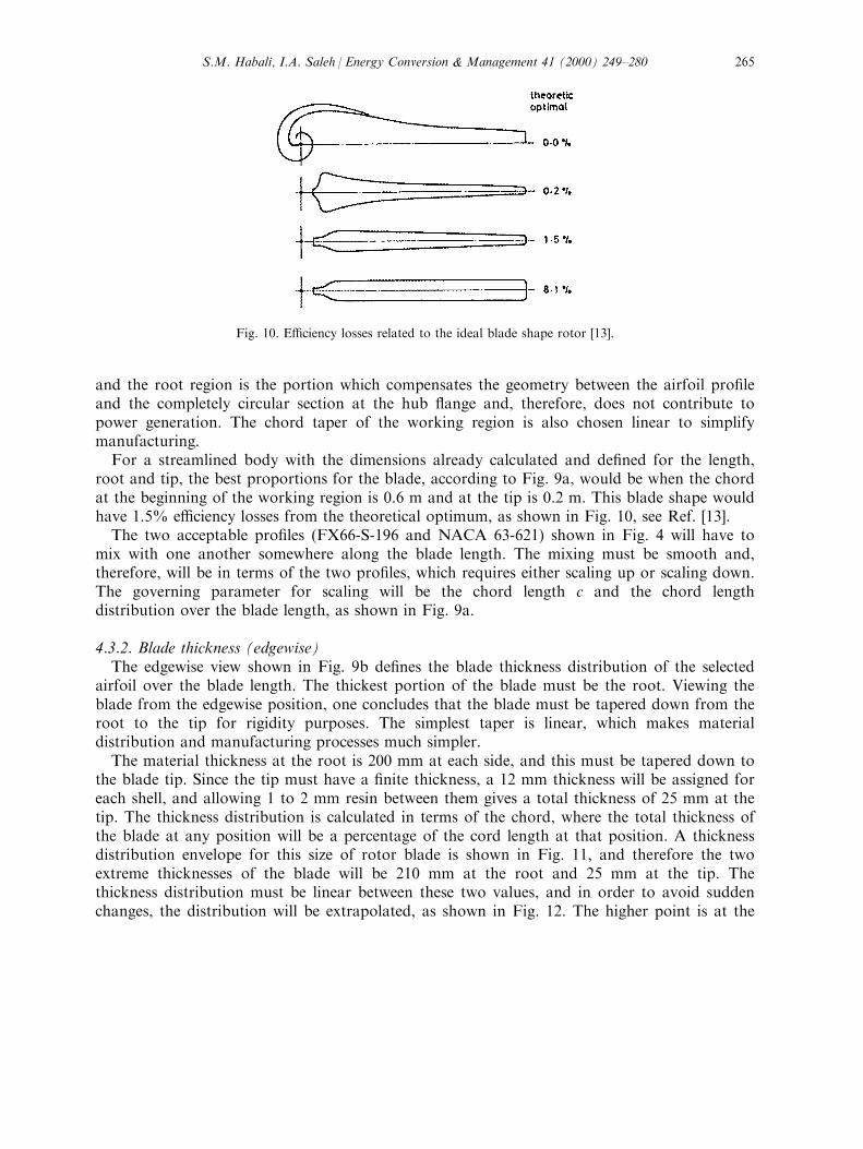
root and tip, the best proportions for the blade, according to Fig. 9a, would be when the chordat the beginning of the working region is 0.6 m and at the tip is 0.2 m. This blade shape wouldhave 1.5% e�ciency losses from the theoretical optimum, as shown in Fig. 10, see Ref. [13].The two acceptable pro®les (FX66-S-196 and NACA 63-621) shown in Fig. 4 will have to

mix with one another somewhere along the blade length. The mixing must be smooth and,therefore, will be in terms of the two pro®les, which requires either scaling up or scaling down.The governing parameter for scaling will be the chord length c and the chord lengthdistribution over the blade length, as shown in Fig. 9a.

4.3.2. Blade thickness (edgewise)The edgewise view shown in Fig. 9b de®nes the blade thickness distribution of the selected

airfoil over the blade length. The thickest portion of the blade must be the root. Viewing theblade from the edgewise position, one concludes that the blade must be tapered down from theroot to the tip for rigidity purposes. The simplest taper is linear, which makes materialdistribution and manufacturing processes much simpler.The material thickness at the root is 200 mm at each side, and this must be tapered down to

the blade tip. Since the tip must have a ®nite thickness, a 12 mm thickness will be assigned foreach shell, and allowing 1 to 2 mm resin between them gives a total thickness of 25 mm at thetip. The thickness distribution is calculated in terms of the chord, where the total thickness ofthe blade at any position will be a percentage of the cord length at that position. A thicknessdistribution envelope for this size of rotor blade is shown in Fig. 11, and therefore the twoextreme thicknesses of the blade will be 210 mm at the root and 25 mm at the tip. Thethickness distribution must be linear between these two values, and in order to avoid suddenchanges, the distribution will be extrapolated, as shown in Fig. 12. The higher point is at the

Fig. 10. E�ciency losses related to the ideal blade shape rotor [13].


edge of the steel ¯ange, where this ¯ange should have a curvature (outward) at the end toavoid stress concentration rises. The lower point, however, cannot fall on the blade because thetip will be chamfered to remove sharp edges for better aerodynamic performance.

4.3.3. Pro®le mixing (pro®le matching)From the pro®le system designation, the two selected pro®les (NACA 63-621) and (FX 66-S-

196) have maximum thicknesses of 21 and 19.6% of chord, respectively. In order to match anairfoil pro®le to any given thickness, the pro®le thickness is simply multiplied by a certainpercentage that makes it match that thickness. In this design, the point of mixing the twopro®les was chosen at the beginning of the last third of the blade which should result in a thickblade. At this point, the FX pro®le will be inserted but with a small percentage whichguarantees a smooth transition from the NACA pro®le.

Fig. 11. Envelope of the blade thickness.

Fig. 12. Distribution of the blade thickness over the blade length.


At the next region, however, these percentages will be reversed in favor of the FX pro®le,and depending on the size of the blade, this transition could be carried on for several positions.The following position then will be purely FX pro®le with either a scale up or a scale downfactor. Table 1 lists the blade parameters with the pro®le matching sequence.

4.3.4. Twist of the bladeThe twist of the blade is de®ned in terms of the chord line. Blade twist angle is a synonym

for the pitch angle, however the twist de®nes the pitch settings at each position along the bladeaccording to local ¯ow conditions. From the velocity triangle in Fig. 3 and as explained byHabali and Saleh [14], the pitch angle b is large near the root, where the rotational speed (isVt � rO) low and small at the tip where the rotational speed is high. This situation suggests amatch between the twist and rotational speed, since the relative wind velocity W is

W � U� Or �49�Here is a decision to be made:

. ®xing O and searching for the optimum twist b, or

. ®xing b and searching for the optimum O.

The ®rst choice is better because it is easier for designing the gear and the generator. O waschosen to be 75 rpm. As a ®rst estimate of the twist, we use the equation for twist of the zerolift line:

b � ��Rat=r� ÿ at� ÿ k�1ÿ r=R� �50�where at is the angle of attack at the tip and k is a constant such that k > 0. at can becalculated from the velocity triangle shown in Fig. 3 as follows: knowing that O � 75 rpm �2p� 75=60 s � 7:8575 1/s, we obtain a rotational tip speed of Vt � RO � 39:27 m/s. Taking amean free stream wind speed of U = 7 m/s, which is usually taken as a design wind speed [7],

Table 1Complete blade data and pro®le mixing

Station(m)

Chord(mm)

Thickness(mm)

Thickness(%)

Twist(degree)

Pro®le NACA 63-621 = N21, FXS 66-196 = F196

0.8 600 178 29.7 16.0 1.41 (N21)1.2 562 163 29.0 12.8 1.38 (N21)

1.6 524 149 28.4 10.1 1.35 (N21)2.0 486 134 27.6 7.8 1.31 (N21)2.4 448 120 26.8 5.8 1.28 (N21)

2.8 410 105 25.6 4.2 1.22 (N21)3.2 371 91 24.5 2.8 0.85 (N21) + 0.34 (F196)3.6 333 76 22.8 1.8 0.25 (N21) + 0.90 (F196)4.0 295 61 20.7 0.9 1.06 (F196)

4.4 257 47 18.3 0.4 0.93 (F196)4.8 219 32 14.6 0.2 0.74 (F196)5.0 200 25 12.5 0.0 0.64 (F196)


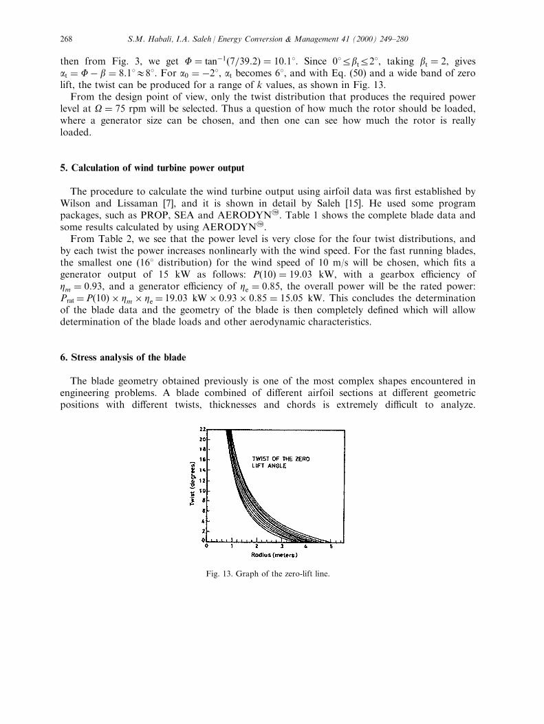
then from Fig. 3, we get F � tanÿ1�7=39:2� � 10:18. Since 08RbtR28, taking bt � 2, givesat � Fÿ b � 8:18188. For a0 � ÿ28, at becomes 68, and with Eq. (50) and a wide band of zerolift, the twist can be produced for a range of k values, as shown in Fig. 13.From the design point of view, only the twist distribution that produces the required power

level at O � 75 rpm will be selected. Thus a question of how much the rotor should be loaded,where a generator size can be chosen, and then one can see how much the rotor is reallyloaded.

5. Calculation of wind turbine power output

The procedure to calculate the wind turbine output using airfoil data was ®rst established byWilson and Lissaman [7], and it is shown in detail by Saleh [15]. He used some programpackages, such as PROP, SEA and AERODYN2. Table 1 shows the complete blade data andsome results calculated by using AERODYN2.From Table 2, we see that the power level is very close for the four twist distributions, and

by each twist the power increases nonlinearly with the wind speed. For the fast running blades,the smallest one (168 distribution) for the wind speed of 10 m/s will be chosen, which ®ts agenerator output of 15 kW as follows: P�10� � 19:03 kW, with a gearbox e�ciency ofZm � 0:93, and a generator e�ciency of Ze � 0:85, the overall power will be the rated power:Prat �P�10� � Zm � Ze � 19:03 kW� 0:93� 0:85 � 15:05 kW. This concludes the determinationof the blade data and the geometry of the blade is then completely de®ned which will allowdetermination of the blade loads and other aerodynamic characteristics.

6. Stress analysis of the blade

The blade geometry obtained previously is one of the most complex shapes encountered inengineering problems. A blade combined of di�erent airfoil sections at di�erent geometricpositions with di�erent twists, thicknesses and chords is extremely di�cult to analyze.

Fig. 13. Graph of the zero-lift line.


Therefore, an approximate solution using the Finite-Element Method (FEM) will be anultimate choice of solution.

6.1. Blade aerodynamic forces (blade loadings)

The blade geometry obtained previously forms the main data necessary to formulate a modelin order to calculate the aerodynamic forces and other data, such as the operating parameters.The procedure for calculating the aerodynamic blade loadings is shown in detail by Saleh [15].For these calculations, the programs:

. LOADS (developed at Oregon State University in 1980 to analyze blade loads for rigidrotors of simple geometry including ¯apwise ¯exing and unsteady aerodynamics, withoutyawing and without pitch variations), see Ref. [1].

. YawDyn for yaw considerations [16], and

. MOSTAB, SEACC and AERODYN

were used. The data input to the program will be the blade geometry, as shown in Table 1, andthe programs will be run for a range of wind speeds and pitch angle, in addition to twelvedi�erent yaw positions. Table 3 gives the values of the force and moment components actingon the blade during operation at a maximum wind speed of 25 m/s and zero-pitch angle(b � 0). Fig. 14 shows all loading types acting on the ¯ying blade.The shear force Vy and the bending moment mx are the dominant components, and,

therefore, will be studied at di�erent settings of pitch angles (08RbR408). Table 4 shows themaximum shear forces and the maximum bending moments for a maximum operating windspeed of 25 m/s and a pitch angle range extending from 08 to 408 in increments of 48. Therotational speed of the rotor is O � 75 rpm. It can be seen from these tables that the shearforce Vy and the bending moment mx reach their maximum values near the blade root forvanishing pitch angle. Much higher loads would occur if the wind is blowing at a skew anglerelative to the blade, which is called the yaw e�ect. Another computer run was made tocalculate the loads resulting from 30 yaw angle, which is considered as the maximum skewencountered during continuous operation.

6.2. Blade reaction forces

For stress analysis purposes, only the force distribution per length (¯apwise) will becalculated because this force represents the maximum load in the most critical direction.

Table 2P (4 m/s), P (10 m/s), and P (16 m/s) for the four-twist distributions

Twist (degree) rpm Pitch (degree) P (4) (kW) P (10) (kW) P (16) (kW)

22 75 0.0 1.06 20.13 23.3820 75 0.0 1.00 19.45 21.9518 75 0.0 0.98 19.50 21.11

16 75 0.0 0.98 19.03 21.22


Furthermore, according to the German DIN, blade loads shall be calculated at an extreme gustof 42 m/s speed. Table 5 shows thrust load (qy) and drag load (qx) distributions over the bladelength for 25 and 42 m/s wind speeds, respectively, and 308 yaw and zero pitch angles. Thisload distribution is plotted in Fig. 15 to show the loading con®guration during the maximumoperating conditions. The area under the curves was also graphically integrated to identify thetotal loads. It is noticed that the reactions to the total load under the 42 m/s curve, i.e., the Fy

(42 m/s) load, represents the load Case 2 studied previously.

6.3. Properties of the blade

6.3.1. Material-mechanical propertiesThe used material is assigned as GRP material with the mechanical properties given in Table

6.

Fig. 14. Aerodynamic loads and moments.

Table 3Blade loads and moments along the blade during normal operation at a maximum wind speed of 25 m/s and zero

pitch angle

Radial position (m) Forces and moments

qx (N/m) qy (N/m) Vx (N) Vy (N) mx (Nm) my (Nm) mc (Nm)

0.00 0.00 0.00 335 1561 1055 5286 0.001.25 140 320 355 1561 612 3334 33741.95 115 346 266 1329 397 2326 2359

2.61 97 373 196 1091 245 1523 15423.23 83 394 140 855 142 923 9313.78 71 401 98 633 76 508 5114.27 63 400 65 473 36 246 246

4.69 57 391 40 273 15 99 995.02 53 374 22 147 4 30 305.26 52 359 9 60 1 5 5

5.40 54 344 1 8 0 0 05.45 0 0 0 0 0 0 0


Table 4Maximum shear forces Vy and maximum bending moment mx for di�erent pitch angles b

Radial position r � z, (m) Vy (N) and mx (Nm) Pitch angle settings b (degree)

0 4 8 12 16 20 24 28 32 36 40

0.0 Vy 1561 1497 1440 1392 1347 1314 1255 1115 893 619 0

mx 5286 5079 4914 4791 4673 4604 4378 3767 2832 1737 8071.25 Vy 1561 1497 1440 1392 1347 1314 1255 1115 893 619 0

mx 3334 3207 3114 3051 2989 2962 2809 2374 1716 964 372

1.95 Vy 1329 1276 1231 1197 1168 1148 1099 971 760 485 170mx 2326 2240 2182 2148 2111 2102 1987 1645 1138 577 168

2.61 Vy 1091 1048 1016 996 978 966 926 809 596 338 153mx 1523 1469 1438 1420 1400 1401 1315 1054 687 304 48

3.23 Vy 855 823 803 793 781 755 746 626 423 209 111mx 923 893 877 869 857 864 799 611 373 163 ÿ4

3.78 Vy 633 612 601 597 586 589 561 437 273 110 57

mx 508 492 485 481 475 484 433 314 179 48 ÿ154.27 Vy 437 423 418 415 407 417 381 276 159 45 0

mx 246 239 236 232 232 237 202 140 74 11 ÿ114.69 Vy 273 266 262 259 256 266 226 155 81 11 ÿ9

mx 99 96 95 93 95 95 77 51 25 1 ÿ55.02 Vy 147 143 142 138 141 142 113 74 35 ÿ1 ÿ17

mx 30 29 29 28 29 28 22 14 6 ÿ1 ÿ25.26 Vy 60 58 58 56 60 55 42 27 12 ÿ2 ÿ21

mx 5 5 5 5 5 5 3 2 1 0 05.40 Vy 8 8 8 8 9 7 6 3 1 0 ÿ21

mx 0 0 0 0 0 0 0 0 0 0 05.45 Vy 0 0 0 0 0 0 0 0 0 0 0

mx 0 0 0 0 0 0 0 0 0 0 0

Table 5Blade loads qx (N/m) and qy (N/m) distributions for: 25 and 42 m/s wind speeds and 308 yaw and 08 pitch angles

Radial position R � z, (m) qy (25 m/s) (N/m) qx (25 m/s) (N/m) qy (42 m/s) (N/m) qx (42 m/s) (N/m)

0.00 0.0 0.0 0.0 0.0

1.25 395 200 908 4141.95 468 182 996 3362.61 531 166 1047 276

3.23 578 152 1062 2273.78 603 139 1043 1894.27 611 130 1003 162

4.69 598 121 948 1425.02 557 107 886 1295.26 531 103 833 1235.40 513 109 791 124

5.45 0.0 0.0 0.0 0.0


6.3.2. Blade-mass propertiesThe blade-mass properties are calculated and given in Table 7. The second moments of area

(Ix�z� and Iy�z�) distribution over the blade length is shown in Fig. 16. Furthermore, the fourcritical sections of the blade are shown in Fig. 17.

6.4. Finite element modeling

6.4.1. Geometric solid modelingIn order to utilize FEM, a solid model for the blade must be created ®rst to de®ne the

surface boundaries and domain contained in it. The contained domain will determine the shapeand the number of elements that could be used in the analysis. The solid model is created inARIES in three steps as mentioned by Saleh [15]. One of the most powerful solid modelers isthe ARIES Mechanical Computer Aided Engineering Design (MCAED) software used by theRenewable Research Center (RERC) at the Royal Scienti®c Society. This package was

Fig. 15. Con®guration of load distribution for 25 and 42 m/s wind speeds.

Table 6

GRP mechanical properties

Density r � 1:4� 10ÿ6 kg/mm3

Tensile yield strength syt � 63 MPaUltimate tensile strength su � 129 MPa

Modulus of elasticity E � 6 GPaCompressive strength syc � 170 MPaShear modulus G � 2:5424 GPaPoisson's ratio n � 0:18Glass content c = 50%


developed by ARIES Technology in Lowell, Massachusetts, USA, for mechanical engineeringdesign and analysis. The FEM model consists of three phases, as shown in Fig. 18 and in AriesTechnology (1993) [17]. The modeling is the preprocessing phase of the ®nite element process,which includes geometry creating, de®nitions of loading and restraining conditions andconstructing of an e�cient mesh.Taking the maximum loads on the blade at 42 m/s from Table 5 and Fig. 15, we get a

maximum thrust load (¯apwise) of Fy,root � 4:82 kN applied at the aerodynamic center of theblade, which is located at 0:5Lb � 0:5� 5:45 m � 2:725 m. Then, at the root section, we have:

. the thrust force Fy,root � 4:517 kN,

. the moment Mx,root�4:82 kN� 2:5333 m�11:443 kN m,

. the drag force Fx,root � 1:023 kN, and

. the moment My,root � 1:023 kN � 2.5333 m = 2.592 kN m.

Table 7Blade mass properties

Weight = 1156.87 N Mass = 117.97 kgVolume = 8.4263 � 107 mm3 Density = 1.4 � 10ÿ6 kg/mm3

Area = 7.4522 � 106 mm2

Properties with respect to origin at the hub

Ox � 0:0 Oy � 0:0 Oz � 0:0Mass moment of inertia (kg/mm2)Ix � 2:544� 108 Iy � 2:560� 108 Iz � 2:172� 106

Center of gravity (mm)Cgx � 44:27 Cgy � 17:59 Cgz � 1668Root cross sectional area propertiesAroot = 18800 mm2 Ix,root � 70:844� 106 mm4 Iy,root � 55:374� 106 mm4

Fig. 16. Distribution of second moments of inertia Ix and Iy along the blade.


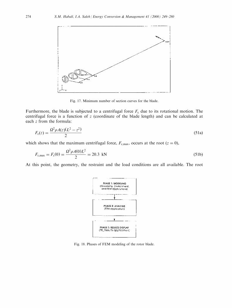
Furthermore, the blade is subjected to a centrifugal force Fc due to its rotational motion. Thecentrifugal force is a function of z (coordinate of the blade length) and can be calculated ateach z from the formula:

Fc�z� � O2rA�z��L2 ÿ z2�2

�51a�

which shows that the maximum centrifugal force, Fc,max, occurs at the root (z � 0),

Fc,max � Fc�0� � O2rA�0�L2

2� 20:3 kN �51b�

At this point, the geometry, the restraint and the load conditions are all available. The root

Fig. 17. Minimum number of section curves for the blade.

Fig. 18. Phases of FEM modeling of the rotor blade.


region geometry is meshed using a TETRAHYDRON element of four nodes and three degreesof freedom at each node (ux,uy,uz), see Fig. 19. The modeled region contains 1103 nodes and3867 elements. The model, at this point, is considered complete and ready to be submitted tothe built-in module of the well known FE package ANSYS within ARIES in order to beanalyzed. This is the second phase of the FE modeling which is the processing phase. Fig. 20shows the forces at the root region as a computer output.The third and the last phase of the FE modeling is the results display which is the post

processing phase. The most important output required here is the displacements and stressesresulting from the applied loads. Fig. 21a shows the forces and the moments whereas Fig. 21bshows the stress distribution at the root section.

7. Results and discussion

7.1. Stress, strain and de¯ection

The results of the analysis using FEM are displayed after completing the calculation. Theresults indicate a maximum (principal) stress of smax � 9:348 N/mm2 = 9.348 MPa occuring atthe tension side of the root cross section of the blade. Comparing this stress with sy,GRP � 63MPa gives a factor of safety of 6.7. This principal stress is also compared with the root stresssroot � 45 MPa calculated previously for a factor of safety of 2. The di�erence between the tworesults (smax and sroot) is due to the centrifugal and drag forces added to the model by the FEanalysis and the additional cross sectional area at the root section represented by therectangular spar at the blade center. The stress distribution over the blade length is di�cult tobe plotted since each ®ber has its own stress distribution. Generally, we can say the stress szshows a decreasing nonlinear variation over the blade length. However, the stress distributionover the root cross section is shown in Fig. 21b.

Fig. 19. Tetrahydron element of four nodes with three degrees of freedom (ux,uy,uz) per node.


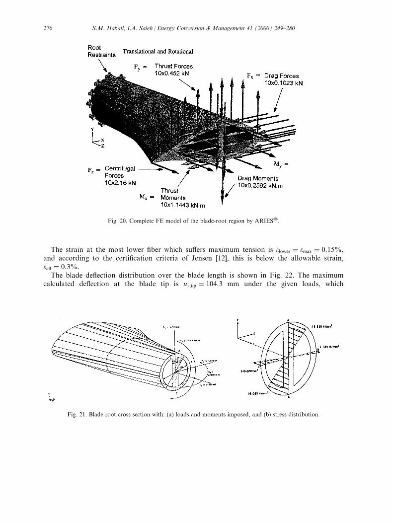
The strain at the most lower ®ber which su�ers maximum tension is elower � emax � 0:15%,and according to the certi®cation criteria of Jensen [12], this is below the allowable strain,eall � 0:3%.The blade de¯ection distribution over the blade length is shown in Fig. 22. The maximum

calculated de¯ection at the blade tip is uy,tip � 104:3 mm under the given loads, which

Fig. 20. Complete FE model of the blade-root region by ARIES2.

Fig. 21. Blade root cross section with: (a) loads and moments imposed, and (b) stress distribution.


concludes the analysis by insuring enough margin for safety of the design especially duringextreme operating situations.In order to analyze the FEM solution, simple straight forward bending strength calculations

will indicate its accuracy. This is accomplished through using the ¯exure formula for thecombined loadings

sz�x,y,z� � Fc

Az2

Myx

Iy2

Mxy

Ix�52�

where the positive sign corresponds to tension and the minus sign to compression. The rootcross section shown in Fig. 21a has the properties:

Ix,root � pÿd 4

o ÿ d 4i

�64

� bh3

12� 70:8440308� 106 mm4

Iy,root � pÿd 4

o ÿ d 4i

�64

� hb3

12� 55:374030� 106 mm4

and

Az,root � 18800 mm2:

Thus, Eq. (52) provides the stress distribution over the root cross section:

sz,root�x,y� � �1:079824:9142x216:9600y

Fig. 22. Curve-®t extrapolation of blade de¯ection (uy) during extreme operating conditions at 42 m/s wind speed.


The sense of the forces and moments shown in Fig. 21a determines the signs of the stresses.This stress represents a complex surface that extends over the root cross sectional area.Therefore, the outer-most ®ber stresses at points A, B, C and D of the root cross section,shown in Fig. 21b, are:

sA � ÿ15:835 MPa

sB � ÿ3:789 MPa

sC � �18:085 MPa

sD � �6:040 MPa:

The maximum tensile stress is sC � 18:085 MPa occuring at point C, which is much lower thansyt,GRP � 63 MPa with a factor of safety of 3.5. The maximum compressive stress is sA �15:835 MPa occurring at point A, which is much lower than sYC,GRP � 170 MPa, with a factorof safety of 10.7.The results obtained by the FEM solution gave the maximum (principal) stress as 9.3487

MPa which certainly falls within the stress distribution shown in Fig. 21b. The reason for thedi�erence between the FEM results and the foregoing analysis results is that in the later one,concentrated load representation was used at the root to represent the actual distributedaerodynamic loads.From the previous discussion, two conclusions can be obtained:

1. The FEM solution is satisfactory and acceptable.2. The blade material for the given root design can withstand the applied loads with enough

safety margin.

8. Conclusions and recommendations

. Rotor inertia has a great e�ect on power production, where during start up before reachingthe cut in speed, the rotor requires higher torque to start turning and production but muchless torque is needed to produce the same unit power after it has run up to full speed.

. The necessary data for evaluation of the rotor blade performance can be produced by theresults of measurements. The power curve is the most important piece of information. For apitch regulated wind turbine, the performance of this design of GRP blades can only be seenin the part of the power curve up to the rated power of 15 kW at 10 m/s. Beyond this point,the performance of the blade is overshadowed by the control system which dumps all excesspower (over the rated), thereby indicating a decrease in e�ciency as indicated by the Cp±lcurve.

. The wind shear (horizontal or vertical) has also an e�ect on the strength of the blade. Thise�ect is more clear with large rotors, but it still has a markable in¯uence on small turbines.


. For a fully satisfactorily analysis using the FEM, large computers with very advancedsoftware have to be used. Automatic mesh generation and satisfactory solutions have to beexamined.

. For fully understanding the mechanical behaviour of the rotor blades, tests should beperformed by conducting a thorough fatigue test program, which is usually characterized bybeing costly and time consuming.

. Since the blade root exhibited durability and resilience during testing and operation, it isrecommended that the design of the blade root be more theoretically investigated using thetheory of elasticity for anisotropic composite materials in three dimensions.

. It is recommended that other pro®les and other composite materials for other wind regimesbe studied.

References

[1] Harten JR. Evaluation of prediction methodology for blade loads on a horizontal axis wind turbine. In: NinthASME Wind Energy Symposium, SED-9:. New Orleans, LA, January 14±18. 1990. p. 105±10.

[2] Park J. Simpli®ed wind power systems for experimentation. Brownsville, CA: Hellion Inc, 1975.[3] Jackson KL, Migliore PG. Design of wind turbine blades employing advanced airfoils. In: West Wind Industry,

Inc., Windpower-87 Conference. San Francisco, CA, October. 1987.

[4] Lysen EH. In: 2nd ed, Introduction to wind energy, CWD 82-1. Netherlands: Amersfort, 1983.[5] Tangler J, Smith B, Jager D, Olson, T. Atmospheric performance of the special-purpose SERI thin-airfoil

family, Final results. Solar Energy Research Institute, 1817 Code Blvd., Golden, CO., Presented at ECWEC 90,

Madrid, 1990.[6] Davidson R. Danes to test run new american blades. Windpower monthly.[7] Wilson RE, Lissaman PBS. Applied aerodynamics of wind power of wind power machines. National Science

Foundation. Under Grant No. GI-41840, Oregon State University, OR, May, 1974.[8] Prandtl L. Appendix to wind turbines with minimum energy losses. In: Betz A, editor. Goettenger News,

Goettenger, 1919, pp. 193±217.[9] Miley SJ. A catalog of low Reynolds number airfoil data for wind turbine applications, USDOE, Wind Energy

Tech. Division, Report-3387, UC-60, February, 1982.[10] Mikhail AS. Wind power for developing nations. USDOE, Wind Tech. Division, SERI/ TR-762-966, UC

Category: 60, July, 1980.

[11] Ta'ani R, Amr M, Saleh I. Water pumping from deep wells by using Aeroman 12.5/14 wind energy converter.In: 16th International Sonnenforum, Berlin 2. DGS-Sonnenenergie Verlag GmbH, Muenchen, Germany,August 22±September 2. 1988.

[12] Jensen PH. Static test of wind turbine blades. Test station for wind mills, Risoe National Laboratory, Roskilde,Denmark, April, Jensen PH, Krogsgaard J, Lundsger P, Rasmussen F. Fatigue testing of wind turbine blades.EWEA Conference and Exhibition, Rome, Italy, October, 1986.

[13] Moment R, Pastore J. Wind energy conversion. In: A Short Seminar Presented to the Royal Scienti®c Society

by Rocky Flats Wind Energy Research Center, Rockwell International Corporation, USAID, March. 1984. p.10±4.

[14] Habali SM, Saleh IA. Pitch control criteria for small wind turbines. In: Proceedings of the 1992 International

Renewable Energy Conference, 2:. University of Jordan, Amman, Jordan. 1992. p. 459±559.[15] Saleh I. Testing and performance of locally manufactured glass ®ber wind turbine blade. Master thesis, College

of Engineering and Technology, University of Jordan, Amman, Jordan. March, 1994.


[16] Hansen AC, Cui X. A summary of experiences in the analysis of rigid rotor yaw control systems. In: NinthASME Wind Energy Symposium. SED-9:. ASME, NY, January. 1990. p. 181±7.

[17] Aries Technology, Inc. Finite element modeling reference manual, P/N2806301, Aries Technology, Inc., 600Su�olk Street, Lowell, Masschusetts 01854, 1993.


diseño aerogenerador1

Documents

rotor blade

local design

small blades

x directionfy force

abstractwind energy

y directionfz force

x directioncy force

theaerodynamic design