disi - university of trento algorithms and performance
TRANSCRIPT

PhD Dissertation
International Doctorate School in Information and
Communication Technologies
DISI - University of Trento
ALGORITHMS AND PERFORMANCE ANALYSIS FOR
SYNCHROPHASOR AND GRID STATE ESTIMATION
Grazia Barchi
Advisor:
Prof. Dario Petri
University of Trento
January 2015


Dedicated to everyone I love,
especially to my two grandmothers


Abstract
The electrical quantities of future power networks are expected to exhibit strong fluc-
tuations caused by dynamic bidirectional energy flows transferred from/to a multitude
of “prosumers”. Such variations have to be accurately measured in real-time either for
efficient power distribution or for safety and protection purposes. This task can be ac-
complished by the Phasor Measurement Units (PMUs), which measure the phasor of
voltage or current waveforms synchronized to the Coordinated Universal Time (UTC).
Accuracy of synchrophasor measurements is one of the many open challenges that need to
be addressed in order to guarantee smart grid reliability and availability. Synchrophasor
measurement has gained an undisputed relevance in the research community working on
power delivery issues for various reasons. Among them, state estimation (SE) of both
transmission and distribution networks is one of the most important. Within this general
context, this dissertation covers two complementary topics.
In the first part, starting from the concept of synchrophasor and from the definition of
the parameters to evaluate PMU performances, useful guidelines to design a filter-based
synchrophasor estimator are provided. Afterwards, an extensive performance comparison
of some state-of-the-art synchrophasor estimation algorithms is reported in most of the
static and dynamic conditions described in the IEEE Standards C37.118.1-2011. Also, a
novel technique able to address both static and dynamic disturbances is presented and
analyzed in depth. In this respect, special attention is devoted to phasor angle estimation
accuracy, which is particularly important for active distribution networks.
The second part of the dissertation is focused on the role and the impact of PMUs
for grid state estimation. After recalling the state estimation problem and the traditional
Weighted Least Square (WLS) technique to solve it, a general uncertainty sensitivity
analysis to different types of measurements is introduced and justified both theoretically
and through simulations. Afterwards, the effect of a growing number of PMUs on WLS-
based state estimation uncertainty is evaluated as a function of instrumental accuracy
and line parameters tolerance. Finally, a Bayesian linear state estimator (BLSE) based
on a linear approximation of power flow equations for distribution networks is presented.
The main advantage of BLSE is that in most cases it is so accurate as the WLS technique,
but it is computationally lighter, faster and more stable from the numerical point of view.
Keywords– Phasor Measurement Unit, synchrophasor estimation, state estimation, power
system measurement, uncertainty.


Acknowledgements
This work is the conclusion of three years of passionate research, which has involved also
several other people.
First of all, I would like to express my gratitude to my advisor, Prof. Dario Petri, for
his guidance and motivation during the whole PhD program. I would like to thank Dr.
David Macii and Dr. Daniele Fontanelli for their suggestions and precious support.
Special thanks goes to Prof. Kameshwar Poolla and to Prof. Alexandra von Meier for
the opportunity that they gave me to be a visiting scholar at the University of California,
Berkeley; and to Prof. Luca Schenato, Dr. Reza Arghandeh and Dr. Guido Cavraro for
the fruitful scientific collaboration while I was there.
Finally, I would like to thank my family and my friends for their endless support and
the colleagues who I have met in these years.
Grazia


Publications as author and co-author
International Journals
[J.1 ] G. Barchi, D. Fontanelli, D. Macii and D. Petri, “On the Accuracy of Phasor
Angle Measurements in Power Networks”, on IEEE Trans. Instrumentation and
Measurement,vol., no., pp., . 2015
[J.2 ] G. Barchi, D. Macii, D. Belega and D. Petri, “Performance of synchrophasor
estimators in transient conditions: A comparative analysis”, IEEE Trans. Instru-
mentation and Measurement,vol.62, no.9, pp.2410-2418, Sept. 2013
[J.3 ] G. Barchi, D. Macii and D. Petri, “Synchrophasor Estimators Accuracy: A Com-
parative Analysis,” IEEE Trans. Instrumentation and Measurement,vol.62, no.5,
pp.963-973, May 2013
International Conference Proceedings
[I.1 ] L. Schenato, G. Barchi, D. Macii, R. Arghandeh, K. Poolla and A. Von Meier,
“Bayesian Linear State Estimation using Smart Meters and PMUs Measurements
in Distribution Grids,” IEEE International Conference on Smart Grid Communica-
tions 2014, pp. 1-6, Venice, Italy, 3-6 Nov 2014.
[I.2 ] D. Macii, G. Barchi and D. Petri,“Uncertainty Sensitivity Analysis of WLS-based
Grid State Estimators,” IEEE International Workshop on Applied Measurements for
Power Systems, pp. 1-6, Aachen, Germany, 24-27 Sep 2014.
[I.3 ]D. Macii,G. Barchi and L.Schenato, “On the Role of Phasor Measurement Units
for Distribution System State Estimation,” IEEE Workshop on Environmental,
Energy and Structural Monitoring, pp. 1-6, Naples, Italy, 17-18 Sep 2014.
[I.4 ]G. Barchi, D. Fontanelli, D. Macii and D. Petri, “Frequency-domain Phase Mea-
surement Algorithms for Distribution Systems,” IEEE International Instrumenta-
tion and Measurement Technology Conference (I2MTC), pp. 1828-1833, Montev-
ideo, Uruguay, 12-15 May 2014.
[I.5 ]G. Barchi, D. Macii, and D. Petri, “Phasor Measurement Units for Smart Grids:
Estimation Algorithms and Performance Issues”, AEIT Meeting 2013, Oct. 2013.
[I.6 ]D. Macii, G. Barchi and D. Petri, “Design Guidelines of Digital Filters for Syn-
chrophasor Estimation”, IEEE International Instrumentation and Measurement Tech-
nology Conference (I2MTC), pp.1579-1584, May 2013.

[I.7 ]G. Barchi, D. Macii and D. Petri,“Effect of transient conditions on DFT-based
synchrophasor estimator performance”, IEEE International Workshop on Applied
Measurements for Power Systems (AMPS), pp. 1-6, Sep. 2012.
[I.8 ] G. Barchi and D. Petri,“An improved dynamic synchrophasor estimator”, IEEE
International Energy Conference and Exhibition (ENERGYCON), pp. 812-817, Sep.
2012.
[I.9 ]G. Barchi, D. Macii and D. Petri, “Accuracy of One-cycle DFT-based Synchropha-
sor Estimators in Steady-state and Dynamic Conditions”, IEEE International In-
strumentation and Measurement Technology Conference (I2MTC), pp. 1529-1534,
May 2012.
i

ii

Contents
1 Introduction 1
1.1 Context of the research . . . . . . . . . . . . . . . . . . . . . . . . . . . . . 1
1.2 Objectives and contribution of the research work . . . . . . . . . . . . . . . 4
2 Synchrophasors and PMUs 7
2.1 Phasor Measurement Unit . . . . . . . . . . . . . . . . . . . . . . . . . . . 7
2.2 Concept of synchrophasor in the series of standards
IEEE C37.118-2011 . . . . . . . . . . . . . . . . . . . . . . . . . . . . . . . 9
2.2.1 Synchrophasor, frequency and ROCOF definitions . . . . . . . . . . 10
2.2.2 Measurement evaluation . . . . . . . . . . . . . . . . . . . . . . . . 12
2.3 Reference signal processing models . . . . . . . . . . . . . . . . . . . . . . 13
2.3.1 P-Class filter model . . . . . . . . . . . . . . . . . . . . . . . . . . . 15
2.3.2 M-Class filter model for phasor . . . . . . . . . . . . . . . . . . . . 15
2.4 Proposed guidelines for filter-based
synchrophasor estimation . . . . . . . . . . . . . . . . . . . . . . . . . . . . 16
2.4.1 Filter design criteria . . . . . . . . . . . . . . . . . . . . . . . . . . 16
2.4.2 Simulation Results . . . . . . . . . . . . . . . . . . . . . . . . . . . 20
2.5 Conclusion . . . . . . . . . . . . . . . . . . . . . . . . . . . . . . . . . . . . 25
3 Synchrophasor Estimation Algorithms 27
3.1 Literature overview . . . . . . . . . . . . . . . . . . . . . . . . . . . . . . . 27
3.2 Analyzed Synchrophasor Estimators . . . . . . . . . . . . . . . . . . . . . . 28
3.3 Accuracy performance analysis . . . . . . . . . . . . . . . . . . . . . . . . . 32
3.3.1 Effect of static off-nominal frequency-offset . . . . . . . . . . . . . . 32
3.3.2 Effect of amplitude and phase modulation . . . . . . . . . . . . . . 35
3.3.3 Effect of harmonics . . . . . . . . . . . . . . . . . . . . . . . . . . . 40
3.3.4 Effect of wideband noise . . . . . . . . . . . . . . . . . . . . . . . . 42
3.4 Transient performance analysis . . . . . . . . . . . . . . . . . . . . . . . . 45
3.4.1 Amplitude Step Change . . . . . . . . . . . . . . . . . . . . . . . . 46
iii

3.4.2 Phase Step Change . . . . . . . . . . . . . . . . . . . . . . . . . . . 51
3.4.3 Linear Frequency Ramp . . . . . . . . . . . . . . . . . . . . . . . . 52
3.5 Conclusion . . . . . . . . . . . . . . . . . . . . . . . . . . . . . . . . . . . . 54
4 A Dynamic DFT-based Synchrophasor Estimator 57
4.1 Interpolated Dynamic DFT IpD2FT estimator . . . . . . . . . . . . . . . . 57
4.2 Computational Complexity . . . . . . . . . . . . . . . . . . . . . . . . . . . 61
4.3 Simulation results . . . . . . . . . . . . . . . . . . . . . . . . . . . . . . . . 61
4.3.1 Accuracy performance analysis . . . . . . . . . . . . . . . . . . . . 62
4.3.2 Transient performance analysis . . . . . . . . . . . . . . . . . . . . 66
4.4 The problem of Phasor Angle Estimation . . . . . . . . . . . . . . . . . . . 70
4.4.1 Simulation and results . . . . . . . . . . . . . . . . . . . . . . . . . 71
4.5 Jitter and time alignment uncertainty . . . . . . . . . . . . . . . . . . . . . 81
4.6 Conclusion . . . . . . . . . . . . . . . . . . . . . . . . . . . . . . . . . . . . 83
5 State Estimation and Measurement Uncertainty Sensitivity 85
5.1 Introduction on SE . . . . . . . . . . . . . . . . . . . . . . . . . . . . . . . 86
5.2 Measurement model and observability condition . . . . . . . . . . . . . . . 87
5.3 The WLS state estimator . . . . . . . . . . . . . . . . . . . . . . . . . . . . 89
5.4 Uncertainty Sensitivity Analysis . . . . . . . . . . . . . . . . . . . . . . . . 91
5.5 Uncertainty Sensitivity Optimization . . . . . . . . . . . . . . . . . . . . . 93
5.6 Simulation results . . . . . . . . . . . . . . . . . . . . . . . . . . . . . . . . 96
5.7 Conclusion . . . . . . . . . . . . . . . . . . . . . . . . . . . . . . . . . . . . 100
6 Role of PMU in Distribution System State Estimation 103
6.1 PMUs and State Estimation: an overview . . . . . . . . . . . . . . . . . . 103
6.2 Impact of PMUs on WLS-based State Estimators . . . . . . . . . . . . . . 105
6.2.1 A PMU placement strategy . . . . . . . . . . . . . . . . . . . . . . 105
6.2.2 Simulation Results . . . . . . . . . . . . . . . . . . . . . . . . . . . 106
6.3 An alternative approach for power flow analysis and state estimation . . . 111
6.3.1 Grid model description . . . . . . . . . . . . . . . . . . . . . . . . . 111
6.3.2 Linear power flow computation . . . . . . . . . . . . . . . . . . . . 113
6.3.3 The Bayesian linear state estimator (BLSE) . . . . . . . . . . . . . 115
6.3.4 Simulation Results . . . . . . . . . . . . . . . . . . . . . . . . . . . 117
6.4 Conclusion . . . . . . . . . . . . . . . . . . . . . . . . . . . . . . . . . . . . 119
7 Conclusions 121
iv

A Grid Network parameters 125
A.1 Network 15-bus . . . . . . . . . . . . . . . . . . . . . . . . . . . . . . . . . 125
A.2 IEEE 33-bus . . . . . . . . . . . . . . . . . . . . . . . . . . . . . . . . . . . 127
Bibliography 129
List of Tables 133
List of Figures 133
v


Chapter 1
Introduction
1.1 Context of the research
The worldwide growing demand for electrical energy and, at the same time, the compelling
need for reducing carbon dioxide emissions, have recently created new challenges not
only in the traditional area of energy generation from renewable sources, but also in
power flow control and management. In 2008 the yearly electricity production worldwide
was in the order of about 15,000 billion kWh, but a large increment is envisioned in
the near future especially in those countries (most notably India and China) that have
been experiencing an outstanding economic growth for several years [1]. Of course, the
emissions of carbon dioxide related to energy consumption have enormously grown as
well in the same countries (see Fig. 1.1), thus leading to a significant global increment of
greenhouse gas emissions, in spite of the increasingly aggressive policies for their reduction
in Europe and North America. While, till now, more than 50% of the primary energy
consumption per capita has been due to European or North American users (see Fig. 1.2),
this situation is expected to change drastically in the near future as soon as large masses
of people with improved economic conditions will have steady access to electricity. It is
wellknown that an increasing energy demand, greenhouse gas emission can be reduced
only with a massive deployment of generators based on renewable sources. Even if their
penetration has constantly grown in the last 25 years, especially in Asia as shown in
Fig. 1.3, the way towards a fully sustainable energetic scenario is still very long. In this
context, in industrialized countries the forthcoming widespread deployment of distributed
micro-generators and energy storage elements will turn typical consumers into significant
producers of electrical energy, thus substantially changing the present structure of the
power grid [2]. In particular, the old paradigm based on a few large power plants and
on quite different passive networks for transmission and distribution is expected to be
replaced by active networks in which all the actors involved will enable bidirectional power

2 Introduction
Figure 1.1: Total carbon dioxide emissions from the consumption of energy (millions metric tons) [Source:
Energy Information Administration, U.S. Government]
flows supported by suitable infrastructures for both communication and protection. The
introduction of information and communication technologies (ICT) in the power networks
creates the so-called smart power grids. In the near future the smart grid will allow us
to integrate small production plants and new loads devices (e.g. the electric vehicles)
thus giving to prosumers (producers-consumers) an active role in electricity pricing. At
the same time continuous service, adequate amplitude and frequency stability at the
minimum cost, security, and an acceptable impact on the environment will have to be
ensured and possibly improved. The term continuous service refers mainly to reliability
and availability of the network [3]. Indeed, in the recent years much research work has
focused on solutions to increase transmission capacity with a low environmental impact,
to improve system operation after the integration of variable energy resources (VERs)
such as wind-based or photovoltaic plants [4], and to avoid catastrophic black-outs like
those happened in the North-East of U.S. and in Italy in 2003.
Traditionally, grid monitoring relies on Supervisory Control and Data Acquisition
(SCADA) systems that collect information related to breaker status as well as measure-
ment data of meaningful electrical quantities of the network (such as bus voltages or
injected currents) through Remote Terminal Units (RTUs). On the basis of such data,
various countermeasures can be taken in response to a particular event. Unfortunately,
while a SCADA system typically takes several seconds to support decisions, today some
events require much faster response times. For such reasons, new advanced Wide Area
Monitoring/Measurement System (WAMS) are used for monitoring, protection and con-
trol services.

Context of the research 3
Figure 1.2: Total primary energy consumption per capita (millions Btu per person) [Source: Energy
Information Administration, U.S. Government]
The WAMS is an infrastructure able to acquire data from strategic points of the grid.
The increasing diffusion of Distributed Generation (DG), i.e. small production plants
based on renewable energy sources, requires novel measurement systems and techniques
characterized by a good trade-off between accuracy and responsiveness [5]. For this reason,
in the last years various advanced measurement instruments have been introduced at
the transmission and distribution level in order to reinforce the existing infrastructure.
Among them, the so-called Phasor Measurement Units (PMUs) play a central role in
WAMS. Generally speaking, a PMU is able to measure the phasors of electrical quantities
(i.e. currents or voltages) over intervals of various length synchronized to the Coordinated
Universal Time (UTC) [6]. The reference time is usually provided by a Global Positioning
System (GPS) receiver. Using multiple PMUs in different points allows us to take a
snapshot of the state of the network at a given time. The main advantages of the PMU-
based measurements compared to the conventional current/voltage measurements are:
higher accuracy in both magnitude and phase, availability of synchronous data and fast
reporting rates (i.e. ranging between about 10 Hz and 100 Hz). Unfortunately, such high
rates (which are expected to grow further in the future) require to store and to manage
huge amounts of data, thus creating serious scalability issues due to the data tsunami that
could affect next-generation active distribution networks [7]. Because of this problem and
of other economic or logistic reasons, at the moment the PMUs are supposed just to
support and to complement other traditional measurement techniques, e.g. those based
on smart meters. However, as soon as the active distribution networks will be available
on a wide scale, cheaper PMUs with enhanced functionalities could be used directly to
support multiple applications possibly using the same infrastructure, thus further boosting

4 Introduction
Figure 1.3: Total renewable electricity net generation (Billions kWh) [Source: Energy Information Ad-
ministration, U.S. Government]
the role of this type of instruments. These applications include (but are not limited to)
fast protection equipment (i.e. with response times in the order of few ms) [8], voltage
stability and oscillation monitoring [9, 10], fault detection and location [11], islanding
maneuvers [12, 13], state estimation [14] and load modeling [15].
1.2 Objectives and contribution of the research work
Next-generation PMUs are required to exhibit superior accuracy and responsiveness at
lower costs. Also, they are supposed to measure not only phasors, but also waveform
frequencies and frequency changes. Even if PMU performances are affected by different
uncertainty sources, the estimation algorithm plays an essential role in instrument per-
formance. Several novel estimation techniques have been developed in the last years in
the attempt of both mitigating the effect of static disturbances (such as harmonics and
inter-harmonics) and tracking fast phasor changes due to intrinsic variations of the net-
work operating conditions. Due to the recent definition of various algorithms based on
the so-called phasor dynamic model, a detailed comparison between their performances
can be hardly found in the literature. So one of the primary goals of this research work
is to fill at least partially this gap by presenting and testing quite famous estimation
algorithms in a common and widely accepted framework: the conditions described in the
IEEE Standards C37.118.1-2011 and its Amendment IEEE C37.118.1a-2014.
In addition, a novel estimator that exhibits high accuracy, good responsiveness and
a reasonable computational complexity is described and analyzed. Special attention will

Objectives and contribution of the research work 5
be devoted to the problem of phasor angle estimation, which is quite unexplored and is
particularly important at the distribution level, where PMU deployment is expected to
be massive in the near future.
The second part of the thesis covers a complementary aspect, namely the role of PMUs
for grid state estimation, which is considered as one of the most relevant applications of
synchrophasor measurements. Many works related to this topic already exist, but most
of them focus on optimal PMU placement to maximize state estimation accuracy or to
minimize the overall monitoring costs. In this thesis instead the emphasis is mainly on how
the number and the accuracy of synchrophasor measurements influence state estimation
especially at the distribution level. At first, a theoretical analysis of the sensitivity to
measurement uncertainty of the well-known Weighted Least Squares (WLS) estimation
technique is reported (properly supported by meaningful simulations) in order to identify
what types of measurements are most critical for state estimation. Thus this analysis paves
the way to a deeper understanding of the impact of PMUs on state estimation uncertainty
in distribution systems. Then, a novel linear Bayesian state estimation algorithm relying
on both PMU-based phasor measurements and real/reactive power pseudo-measurements
is proposed in order to achieve reasonably accurate state estimates with less numerical
problems and with a lower computation burden than using the WLS approach.
In conclusion, the thesis is structured as follows.
Chapter 2 deals with an overview of synchrophasor measurements and PMUs. At first,
the common structure of PMUs is described, along with how the synchrophasor data
are collected. Then, important definitions as well as some static and dynamic testing
conditions based on the IEEE Standard C37.118.1-2011 are introduced. Such testing
conditions will be also used in Chapter 3 and Chapter 4. Finally, some general guidelines
to design a filter for synchrophasor estimation are reported.
In Chapter 3 three state-of-the-art techniques for synchrophasor estimation are de-
scribed and their performances are extensively analyzed and compared under the steady-
state and dynamic conditions reported in the IEEE Standard C37.118.1-2011.
In Chapter 4 a novel synchrophasor estimator is proposed and validated through simu-
lations in most of the conditions reported in the Standard. In view of using this algorithm
in PMUs for distribution systems (where a superior phase measurement accuracy is re-
quired), the phasor angle measurement accuracy alone is analyzed and compared with
the accuracy of other two state-of-the-art algorithms.
In Chapter 5 the problem of state estimation is introduced and the classic static
WLS state estimator is recalled. A sensitivity analysis to measurement uncertainty is
performed to identify which kinds of measurements are preferable for state estimation to
achieve observability when their number is minimum. In this way, the role of PMU-based

6 Introduction
measurements in state estimation with respect to other traditional measurements is also
partially clarified. This aspect is further analyzed in Chapter 6, which investigates more
in depth how a growing number of PMUs and their accuracy affect grid state estimation
accuracy. This analysis, mainly focused on distribution systems, paves the way to the
definition of a novel Bayesian and Linear State Estimation (BLSE) algorithm, which
proves to be faster and more numerically stable than the traditional WLS-based approach.
Finally, Chapter 7 summarizes the main results of the research work and provides an
overview of ongoing and future activities.

Chapter 2
Synchrophasors and PMUs
As stated in Chapter 1, the PMUs are the key elements of the WAMS, as they measure the
phasors of different waveforms over a wide area at the same time. This chapter presents
at first an overview of a common PMU architecture which the specific function of each
block. Then, the main concepts taken from the current synchrophasor Standard IEEE
C37.118.1-2011 and used in the rest of the thesis are introduced. At last some guidelines
to design suitable filters for synchrophasor measurement are proposed.
2.1 Phasor Measurement Unit
The first prototypes of PMUs were built at the Virginia Tech in the early 1980s. At
present, PMUs by different manufacturers may differ in various important aspects. Nonethe-
less, a quite general PMU architecture is shown in Fig. 2.1 [6]. The input waveform, i.e.
Anti-aliasing filter
A/D Converter
PhasorMicro-processor
Phase-lockedoscillator
GPS receiver Modem
Analog inputs
Figure 2.1: A common Phasor Measurement Unit architecture. Source: [6].
Part of this chapter was published in
D. Macii, G. Barchi and D. Petri, “Design Guidelines of Digital Filters for Synchrophasor Estimation”, IEEE
International Instrumentation and Measurement Technology Conference (I2MTC), pp.1579-1584, May 2013.

8 Synchrophasors and PMUs
voltage or current, is acquired by a signal conditioning module (that typically just con-
sists of an anti-aliasing filter), followed by an Analog-to-Digital Converter (ADC). The
sampling clock signal (with a frequency in the order of tens of kilo-samples/second) is
phase-locked with a train of pulses synchronized to the UTC through a GPS receiver or
through wired synchronization protocols such as IRIG-B or the Precision Time Protocol
(PTP) [16]). The digitized electrical waveform is sent to an embedded processing com-
ponent, such as a microprocessor (µP), which calculates the synchronized phasor using a
specific estimation algorithm, frequency and rate of change of frequency (ROCOF). Addi-
tionally, it relies on the synchronization block to time-stamp the measurements. Finally,
the estimated values are transmitted to other PMUs or the Phasor Data Concentrators
(PDCs), which are able to collect data from different PMUs and align their in time. Gen-
erally, four types of files are exchanged between PMUs, i.e. configuration, header and
data files. In addition, command files are used to control the PMUs from a higher level of
the network hierarchy [17]. The PMUs are placed and installed in power system substa-
tions. In order to use PMUs measurement in different applications (e.g. state estimation,
fault detection, stability estimation, control...), they have to be controlled remotely. For
such reasons a hierarchical architecture that involves PMUs, communication systems and
PDC, as shown in Fig. 2.2 has to be realized. The PMUs measurement data can be stored
locally for diagnostic purposes or can be sent to PDCs for high-level filtering and mon-
itoring. Many applications require data from several PMUs. After bad data exclusion,
time-stamps alignment, coherent records are gathered by the PDCs themselves. In order
to extend the PDCs data-gathering capability the Super Data Concentrator or direct (
monitoring system/station) is used at a higher hierarchical level.
PMU
Phasor Data Concentrator
Super Data Concentrator
PMU PMU PMU
Phasor Data Concentrator
Storage Storage
Data storage
Real-time application
Figure 2.2: Phasor measurement systems architecture [6].

Concept of synchrophasor in the series of standardsIEEE C37.118-2011 9
2.2 Concept of synchrophasor in the series of standards
IEEE C37.118-2011
The goal of PMU is to perform real-time and accurate measurements of the phasors
synchronized to the UTC, in order to track possible variations, to detect abnormal phe-
nomena and to support control operations in power grid. However, to operate correctly it
is necessary that synchrophasor measurements and data messaging are compliant with the
definition and the performance requirements of suitable Standards. The synchrophasor
definition was standardized for the first time in 1995 in the IEEE Std 1344. This standard
introduces also concepts such time accuracy, synchronization to UTC and requirements
for waveform sampling. Ten years later, more complete and meaningful changes were in-
troduced in the IEEE Std C37.118-2005. This specifies how to evaluate the measurement
performance and the message structure for synchrophasor data. It defines the Total Vec-
tor Error (TVE) as the main accuracy index and its limits in steady-state conditions in
order to fulfill the compliance requirements. However the need to analyze synchrophasor
performance also under dynamic conditions (i.e in presence of amplitude/phase variations
or frequency ramp) led to the current and revised version in late 2011.
The new standard, IEEE Std C37.118-2011, is divided in two parts: the first one, i.e
IEEE Std C37.118.1-2011 in the following simply called ”the Standard” [18], provides
the definitions of synchrophasor, waveform frequency and rate of change of frequency
(ROCOF). Moreover it deals with the compliance boundaries and tests to evaluate the
performance of PMUs under steady-state and dynamic conditions. The second part,
IEEE Std C37.118.2-2011 deals with the synchrophasor data transfer and data formats
[17]. Two performance classes are defined in the Standard IEEE C37.118.1-2011, i.e. P-
class and M-class, in order to meet orthogonal applicative needs. The P-class PMUs are
mainly oriented to those applications requiring a fast measurement response time (e.g.
for safety-critical, protection purposes). Conversely, the M-class PMUs are used when
measurement accuracy is more important than measurement speed. All the compliance
tests under steady-state and dynamic conditions are specified in the Standard. Recently,
an amendment of the Standard, called IEEE C37.118.1a-2014 was published in order
to fix some inconsistencies and to relax some constraints difficult to meet especially re-
lated to frequency and ROCOF estimation (see 2.2.1). In spite of the recent publication
of Amendment IEEE Std C37.118.1a-2014 in the rest of the dissertation the IEEE Std
C37.118.1-2011 will be considered as reference document, except in the few particular
cases.
According to the Standard, the PMU supports a reporting rate at multiple or sub-
multiples of the nominal frequency. The compliant reporting rate values, expressed in

10 Synchrophasors and PMUs
Frames per second, for 50 Hz and 60 Hz systems are listed in the Tab.2.1. Other reporting
rates(100 frames/s or 120 frames/s or rates lower than 10 frames/s, such as 1 frames/s),
are also encouraged.
Table 2.1: PMU reporting rates[18].
System frequency 50Hz 60 Hz
Reporting rates (Fs - frames per second) 10 25 50 10 12 15 20 30 60
In the following the main concepts introduced in the Standard and used in the rest of
dissertation are presented and explained.
2.2.1 Synchrophasor, frequency and ROCOF definitions
Model signal and synchrophasor
In AC power systems an electrical waveform (i.e. current or voltage) x(t) of nominal
frequency f0 (i.e. 50 Hz or 60 Hz) can be expressed as
x(t) = A cos(2πf0t+ φ) (2.1)
where A is the amplitude and φ is the initial phase. A common representation of (2.1)
through its complex static phasor is defined as
X =A√2ejφ. (2.2)
A synchronized phasor or synchrophasor of an electrical signal in (2.1) is the value X
in (2.2) at a known reference time, tr, synchronized to the Coordinated Universal Time
(UTC) [18]. The convention reported in the Standard for synchrophasor representation is
shown in Fig. 2.3. On the left, the synchrophasor angle is 0 degrees when the maximum
of (2.1) occurs at the UTC second rollover, on the right the synchrophasor angle is –90
degrees when the positive zero crossing occurs at the UTC second rollover.
In steady-state conditions the waveform frequency, amplitude and phase parameters
can be considered as constant during the whole observation interval, while in a more
realistic scenario they are affected by both amplitude and phase variations caused by
power oscillations and other disturbances. So, in order to analyze the behavior of a power
system under both steady-state and dynamic conditions, a generalization of the electrical
waveform model in (2.1) is
x(t) = A[1 + εa(t)] · cos[2πf0(1 + δ)t+ εp(t) + φ] + η(t) (2.3)

Concept of synchrophasor in the series of standardsIEEE C37.118-2011 11
t=0(1 PPS)
𝑋 = 𝐴2
A A
t=0(1 PPS)
𝑋 = 𝐴2 𝑒
−𝑗𝜋2
Figure 2.3: Convention for synchrophasor representation [18].
where A, f0 and φ have the same meaning as in (2.1), 2πδf0t is the accumulated phase shift
due to the static fractional off-nominal frequency offset δ, εa(t) describes the time-varying
amplitude fluctuations, εp(t) includes possible phase fluctuations and η(t) generally in-
cludes possible narrowband components (e.g. harmonics and additive wideband noise).
Since both amplitude and phase in (2.3) change as a function of time, the synchropha-
sor at the UTC reference time tr is defined as
Xr = X(tr) =A(tr)√
2ejϕ(tr) =
A√2
[1 + εa(tr)] · ej[2πf0(1+δ)tr+εp(tr)+φ] (2.4)
Frequency and rate of change of frequency estimation
A last generation PMU is able to measure not only the synchrophasor, but also the
waveform frequency and the rate of change frequency estimation (ROCOF). Starting
from equation (2.3), if εa(·) and η(·) are negligible, the sinusoidal signal can be rewritten
as
x(t) = A cos[ϕ(t)] (2.5)
where ϕ(t) = 2πf0(1 + δ)t+ εp(t) + φ. Thus frequency of signal x(t) in (2.5) at time tr is
defined by
fr = f(tr) =1
2π
dϕ(tr)
dt= f0 + f0δ +
1
2π
dεp(tr)
dt= f0 + ∆f(tr) (2.6)
where ∆f(tr) is the instantaneous deviation frequency from the nominal value. Finally,
the corresponding ROCOF is defined as follow
ROCOFr = ROCOF (tr) =df(tr)
dt=
1
2π
d2ϕ(tr)
dt2=d∆f(tr)
dt(2.7)

12 Synchrophasors and PMUs
Figure 2.4: Graphical representation of TVE definition.
2.2.2 Measurement evaluation
Total Vector Error
The estimation accuracy of the synchrophasor measured by PMU is in the Standard
typically expressed in terms of Total Vector Error (TVE). Indeed, TVE combines the
effect of magnitude errors, phase errors and synchronization uncertainty. If we denote the
estimated phasor as ˆX and the actual phasor value as X, the TVE can be defined as
TV Er =| ˆXr − Xr||Xr|
(2.8)
where the subscript r indicates that both the estimated and the actual value of the phasor
are computed at the reference time tr.
Frequency and ROCOF measurement error
In the last version of the Standard the frequency measurement error and the ROCOF
measurement error are given by the difference between the actual values and the estimated
values. They are defined as
FEr = |fr − fr| = |∆fr −∆fr| (2.9)
RFEr =
∣∣∣∣dfrdt − dfrdt
∣∣∣∣ (2.10)
where the subscript r indicates that both the estimated and the actual value of the phasor
are computed at the reference time tr.

Reference signal processing models 13
TVE[
%]
Time
Step input t=0
response time
1%
Figure 2.5: Example of amplitude step change over the time [18].
Response time and delay time
In order to evaluate the performance of an algorithm when sudden amplitude or phase
change occurs, the Standard suggests to evaluate both the response time and the delay
time. Especially the response time will be used in the following. However both definitions
as they are reported in the Standard are recalled.
The measurement response time “is the time to transition between two steady-state mea-
surements before and after a step change is applied to the input. It shall be determined as
the difference between the time that the measurement leaves a specified accuracy limit and
the time it reenters and stays within that limit when a step change is applied to the PMU
input.[...] Accuracy limits are the TVE, FE, and RFE values for the phasor, frequency,
and ROCOF measurements, respectively”[18]. In the case of TVE (that is the only pa-
rameter considered in next sections) the limit specified by the Standard is set equal to
1%. In Fig. 2.5 an example of TVE response time resulting from an amplitude step is
shown.
The delay time is defined as “the time when the stepped parameter achieves a value that
is halfway between the starting and ending steady-state values”[18].
2.3 Reference signal processing models
Since the PMUs can be made by different manufactures there is no indication in the
Standard on the preferred estimation algorithm. Annex C of IEEE Std C37.118.1-2011
describes a reference signal processing model used to verify the Standard requirements.
However the following disclaimer is also reported in the Standard: “It is given for in-
formation purpose only, and does not imply being the only (or recommended) method for
estimation synchrophasor”[18]. Basically, the phasor estimation model relies on frequency

14 Synchrophasors and PMUs
Antialiasingfilter
ADCAnalog front-end
LP filterW(ω)
LP filterW(ω)
Synchronized Clock to UTC
Quadrature oscillator (f0)
sin 2πf0 cos2πf0
Re
Im
x(t) x[n]
Mag
Ang
Figure 2.6: Block diagram of the synchrophasor estimation model suggested in the Standard IEEE
C37.118.1-2011.
down-conversion and digital low-pass filtering of the in-phase and quadrature components
of voltage and current waveforms. Two examples of low-pass filters having quite different
performances in terms of latency and accuracy are also reported in the same annex: one
for protection-oriented applications (P-class reference model) and the other when high
measurement accuracy is required (M-class reference model). Starting from (2.3), if the
phase fluctuations εp(t) are negligible, but δ 6= 0, then phasor (2.4) rotates at a constant
rate δf0. The block diagram of the basic synchrophasor estimation model described in
Annex C of the Standard is shown in Fig. 2.6 [18]. The expression of the estimator is
ˆXr =
√
2W (0)·∑N−1
2
n=−N−12
w[n]x[r + n] · e−j 2πM (r+n) N odd√
2W (0)·∑N
2
n=−N2
w[n]x[r + n] · e−j 2πM (r+n) N even(2.11)
where:
• x[·] is the digitized input waveform sampled at a rate fs by the front-end analog-to-
digital converter (ADC);
• N is the number of impulse response coefficients of the chosen filter;
• M = fs/f0 represents the number of samples in one nominal waveform cycle. Ac-
cordingly, 2π/M is the angular frequency of the two quadrature digital sine-waves
that are mixed with the input signal;
• w[·] is the impulse response of the adopted low-pass Finite Impulse Response filter;
• W (ν) is the frequency response of the filter, ν = f/fs is the normalized digital
frequency and W (0) is the filter DC gain.
Estimator (2.11) returns the synchrophasor value referred to the observation interval
centered at time tr. Such a timestamp coincides with the sampling instant r/fs, when N

Reference signal processing models 15
is odd, whereas it lies between two subsequent samples (i.e., at time (r − 1/2)/fs), when
N is even. As a consequence, while W (ν) is generally designed to provide a linear phase
response, in (2.11) no phase delay is introduced by the filter (i.e. its phase response is
zero). Notice that if we refer to C = N/M as the number of nominal waveform cycles
in N samples, (2.11) can be equivalently regarded as the C − th sample of the windowed
Discrete-time Fourier Transform of the sequence x[·] centered at time tr. Therefore, the
estimation approach described in [18] and the windowed DFT-based phasor estimators
basically coincide, since the adopted sliding window simply acts as a filter [19].
2.3.1 P-Class filter model
The Annex C suggests a fixed-length two-cycle triangular FIR filter, with an odd number
of samples, regardless of PMU reporting rates. The filter coefficients w[n] are:
w[n] =
(1− 2
N + 2|n|)
(2.12)
where n = −N/2, .., N/2 and N is the filter order. The P-class filter works well at
the nominal frequency when the observation interval matches exactly the period of the
collected sine-wave. However in presence of off-nominal frequency deviations, a magnitude
correction applied to the final phasor is required [18].
2.3.2 M-Class filter model for phasor
The M-class requires that the filter is able to attenuate significantly the signals above the
Nyquist frequency for a given reporting rate. This filter provides more accurate results
in the presence of noise and interfering signals, but with longer reporting delays. In the
amendment to the Standard the filter mask specifications are shown in Fig. 2.7. The
window coefficients can be computed with
w[n] =sin(
2π × 2FfrFsamp
× n)
2π × 2FfrFsamp
× nh[n] (2.13)
where n = −N/2, ..., N/2, N is the filter order, Ffr is the low-pass filter reference frequency
(which depend on the reporting rate), Fsamp is the sampling frequency and h(n) is the
Hamming window sequence.

16 Synchrophasors and PMUs
Figure 2.7: Reference algorithm filter frequency response mask specification for M class [18].
2.4 Proposed guidelines for filter-based
synchrophasor estimation
As shown in paragraph 2.3.1 and 2.3.2, the Standard reports two examples of low-pass
filters with different performances in terms of latency and accuracy. However, no clear
filter design criteria are provided. In [20] and [21] the authors describe and analyze
the performance of two orthogonal filters with time-frequency characteristics that are
particularly suitable for fault location and measurement. In [22] a raised-cosine filter with
a negligible phase distortion is described to halve the phasor estimation delay. In [23] and
[24] two filters for P-class and M-class phasor estimation, respectively, are proposed to
improve the performance of the basic model reported in Annex C of the Standard.
In this section, the same model is used as a starting point to identify optimal filter
design criteria. Some simulation results support the proposed analysis.
2.4.1 Filter design criteria
According to (2.3), an electrical waveform in dynamic conditions can be regarded as an
amplitude and phase modulated signal around a carrier of frequency (1 + δ) · f0. If we
suppose, for the sake of simplicity, that the modulating signals are two sine waves, εa(t)
and εp(t) can be expressed as
εa(t) = ka cos[2πδaf0t+ αa] (2.14)

Proposed guidelines for filter-basedsynchrophasor estimation 17
and
εp(t) = kp cos[2πδpf0t+ αp] (2.15)
where ka (with ka ≤ kaM ) is the amplitude modulation index, δa = fa/f0 is the corre-
sponding fractional frequency, kp (with kp ≤ kpM ) is the amplitude (expressed in radians)
of the phase modulation signal and δp = fp/f0 is the fractional modulation frequency.
Under this assumption, it can be easily proved that the spectrum of (2.3) consists of an
infinite series of monochromatic terms located at frequencies [h·(1+δ)+m·δp+l·δa]·f0, for
h ≤ 1, and l = –1, 0, 1 [25]. This is due to the fact each tone resulting from phase modu-
lation is in turn modulated also in amplitude, thus generating three spectral components
at frequencies (m · δp + l·δa)·f0. The two side terms (i.e., shifted by ±δa·f0 with respect to
m · δp·f0) are proportional to ka. Moreover, the amplitude of each triple of spectral com-
ponents is proportional to Jm(kp), i.e. the first-kind Bessel function of order m computed
at kp. Since the values of |Jm(kp)|, for a given kp, decrease monotonically as a function
of |m|, the effective bandwidth of (2.3) containing 98% of the signal power around the
carrier is 2 · β · f0, with β = (kp + 1)δp + δa [25]. Notice that, in accordance with (2.4),
εa(t) and εp(t) are intrinsically part of the phasor to be estimated, whereas harmonics
in (2.3) represent a disturbance and, consequently, must be suitably filtered to improve
synchrophasor estimation. By mixing the digitized input sequence with two quadrature
sine-waves of nominal frequency f0 (or equivalently, of normalized frequency 1/M), the
fundamental component as well as the modulating terms of (2.3) are down-converted to
the baseband, around frequency δ · f0. Thus, if the static fractional frequency offset δ
lies in the interval [–δM , δM ] (where δM represents the maximum value of the frequency
measurement uncertainty assured by the considered PMU), the one-sided normalized filter
bandwidth that must be used to preserve both static and dynamic phasor contributions is:
BWp =(δp + βM) · f0
fs=δM + (kpM + 1) · δpM + δaM
M, (2.16)
where βM , δaM and δpM denote the maximum allowed values of β, δa and δp, respectively.
Such values can be hardly known a priori. However, for filter design purposes, they can
be set in compliance with the requirements of some standard document such as the IEEE
C37.118.1-2011 and the amendment IEEE C37.118.1a-2014. It is worth noticing that
βM/M is the bandwidth increment needed to track fast phasor fluctuations.
Fig. 2.8 provides a qualitative overview of the main features of the low-pass filter to be
used for phasor estimation after signal down-conversion. Parameters r1 and r2 represent
the maximum ripple amplitudes in the filter pass-band. In general, the flatness in-band
requirements can be relaxed in the frequency interval [±δM/M,±(δM + βM)/M ] (i.e.
r2 > r1), because phase and amplitude fluctuations are expected to be quite small (e.g.,
in the order of 0.1 rad and 10% of phasor nominal amplitude, respectively). Observe that

18 Synchrophasors and PMUs
1M
1 − 2δ𝑀M
1 + 2δ𝑀M
δ𝑀M
𝛽𝑀M
2M
1 + 3δ𝑀M
1 − 3δ𝑀M
2+ δ𝑀M
1 + 𝑟11 − 𝑟11 + 𝑟2
1 − 𝑟2
2 + δ𝑀 + 𝛽𝑀M
Static and dynamic band
Image frequency and 3rd harmonic
2nd harmonic2− δ𝑀M
2 − δ𝑀 − 𝛽𝑀M
𝑟3𝑟4
Figure 2.8: Qualitative representation of the filter design requirements in the frequency domain, including
static and dynamic in-band flatness specifications, second-order and third-order harmonic attenuation and
image tone cancellation.
the transition band of the filter must not exceed (1–2δM)/M . This value corresponds to
the lower end of the frequency interval [(1–2δM)/M, (1+2δM)/M ], where the second-order
signal harmonic lies as a result of signal down-conversion.
In the following, we will refer to r3 as the maximum amplitude of the filter frequency
response in the band [(1–2δM)/M, (1 + 2δM)/M ]. A similar attenuation affects the resid-
ual DC offset of the acquired signal as well, which after down-conversion is located
at normalized frequency –1/M . The frequency band around 2/M deserves some spe-
cial attention, because it includes two different contributions. First of all, the band
[(2–3δM)/M, (2 + 3δM)/M ] contains the down-converted third-order harmonic of the col-
lected signal. In addition, (2 + δ)/M represents the normalized image frequency after
down-conversion. This means that the band [(2−δM–βM)/M,(2+δM+βM)/M ] has exactly
the same spectral content as the band [(–δM–βM)/M, (δM+βM)/M ]. Thus, the magnitude
of the filter frequency response in the band [(2–δM–βM)/M, (2 + δM + βM)/M ] must be
attenuated by a factor r4 r3, in order to make the joint effect of the image compo-
nent and the third-order harmonic negligible on estimation results. worth noticing that
amplitude of the harmonic is generally at most one order of magnitude smaller than the
fundamental. Therefore, if the filter magnitude for ν ≥ (2 + δM + βM)/M is smaller
than r4, the influence of higher-order harmonics on phasor estimation results becomes
negligible. As known, the main performance parameter describing the accuracy of phasor
measurement is the Total Vector Error (TVE) [18]. In particular, if (2.11) is applied to
(2.3) to estimate the dynamic phasor described by (2.4), the following expression holds,

Proposed guidelines for filter-basedsynchrophasor estimation 19
i.e.
TV E =
∣∣∣ ˆXr − Xr
∣∣∣∣∣Xr
∣∣ =
∣∣∣ ˆXb,r + ˆXi,r +∑H
h=2ˆXh,r − Xr
∣∣∣∣∣Xr
∣∣6
∣∣∣ ˆXb,r − Xr
∣∣∣∣∣Xr
∣∣ +
∣∣∣ ˆXi,r
∣∣∣∣∣Xr
∣∣ +H∑h=2
∣∣∣ ˆXh,r
∣∣∣∣∣Xr
∣∣ , (2.17)
where ˆXb,r is the baseband waveform component of the estimated phasor (namely the
component of interest of the input signal), ˆXi,r is the error contribution caused by the
infiltration of the image component and ˆXh,r, for h = 1, · · · , H are the error terms due to
imperfect harmonics filtering. If the phase modulation index is small enough (namely if
kp 1, as it is typically expected in practice), then J0(kp) ≈ 1, |J−1(kp)| = |J1(kp)| < 0.1
and |Jm(kp)| ≈ 0, for m > 1. Therefore, after a few algebraic steps it can be shown that
the following inequality holds, i.e.
| ˆXb,r − Xr || Xr |
< r1+ | r2 − r1 | ·
[kaM
2+
kaM+1
10
](1− kaM )
. (2.18)
As far as the image and harmonic contributions are concerned, it is straightforward to
show that ∣∣∣ ˆXi,r
∣∣∣∣∣Xr
∣∣ +H∑h=2
∣∣∣ ˆXh,r
∣∣∣∣∣Xr
∣∣ ∣∣Xr
∣∣ 6 r4 +r3X2 +
∑Hh=3 r4Xh
X(1− kaM ). (2.19)
If TV Emax represents the maximum tolerable TVE value, the following general design
conditions must be fulfilled:
• 1− r1 ≤ |W (ν)| ≤ 1 + r1 with r1 ≤ F1 · TV Emax for ν ∈[0, δM
M
];
• 1− r2 ≤ |W (ν)| ≤ 1 + r2 with r2 ≤ F2 · TV Emax for ν ∈[δMM, δM+βM
M
];
• |W (ν)| ≤ r3 with r3 ≤ F3 · TV Emax for ν ∈[
1−2δMM
, 2−δM−βMM
];
• |W (ν)| ≤ r4 with r4 ≤ F4 · TV Emax for ν ∈[
2−δM−βMM
,+∞];
• F1 + |F2 − F1| ·
[kaM
2+kaM+1
10
]1−ka + F4 +
F3X2+∑Hh=3 F4Xh
X(1−kaM )≤ 1; (2.20)

20 Synchrophasors and PMUs
where F1, F2, F3 and F4 are adimensional factors that can be used to adjust filter pass-
band and stop-band magnitude, so as to assure that TVE values are smaller than or equal
to TV Emax both in static and dynamic conditions. Evidently, no unique criteria exist to
select the values of fractions F1, F2, F3 and F4.
However, a few rules of thumb can be followed in order to make filter design simpler.
For instance, F2 can be up to one order of magnitude larger than F1, since the value of
kaM in the second term of design conditions above is about 0.1 [18]. This helps relaxing
the flatness filter requirements in the pass-band. The impact of harmonic distortion
depends on the relative amplitude of each harmonic with respect to the fundamental
tone. According to the Standard [18], the relative amplitude of each harmonic till the
50th (i.e. Ah = Xh/X for h = 2, · · · , H, with H = 50 [18]) can be so large as 1% or 10% of
the fundamental tone for P-class and M-class, respectively. As known, the second-order
harmonic is the most critical, but it can be hardly removed due to the narrow transition
band requirements of the filter. Thus, relaxing r3 is essential for filter design feasibility
over reasonably short intervals. Therefore, since 1(1−ka)
≈ 1+kaM the relative contribution
of the second-order harmonic to TVE becomes comparable to F1 if F3 ≈ F1
A2(1+kaM ).
Similarly, the overall joint TVE contribution due to image infiltration and higher-order
harmonics may become comparable to F1 when F4 ≈ F1
(H−2)(1+kaM ) maxh=1,··· ,H
(Ah)+1. Notice
that if the P-class specifications are good enough for the intended application, the TVE
is generally dominated by image infiltration. In the case of M-class requirements instead,
harmonic distortion is typically the main source of estimation uncertainty.
2.4.2 Simulation Results
In order to confirm the validity of the design criteria described in Section 2.4.1, two exam-
ples of filters have been proposed. Such filters do not result from any specific optimization
procedure. Indeed, they have been obtained using known filter design techniques itera-
tively, while checking if condition (2.20) is satisfied a posteriori, but the globally compli-
ance with the Standard is not guaranteed. All simulations have been performed assuming
that fs = 6.4 kHz and M = 128.
Example 1: Two-cycle filter
The accuracy of three two-cycle FIR filters have been compared, i.e.
• a 255-order filter with a triangular impulse response similar to the one suggested in
the Annex C of the Standard IEEE C37.118.1-2011 [18];
• a filter minimizing the effect of phasor image infiltration [19];

Proposed guidelines for filter-basedsynchrophasor estimation 21
Amplitude[dB]
Normalized frequency (ν)
𝛽𝑀𝑀
𝛿𝑀 + 𝛽𝑀𝑀 1 + 2𝛿𝑀
𝑀2 − 𝛿𝑀 − 𝛽𝑀
𝑀
𝑟4
𝑟31 ± 𝑟1
1 ± 𝑟2
Figure 2.9: Frequency response magnitude of an equiripple FIR filter potentially compliant with the
P-class requirements specified in the Standard IEEE C37.118.1-2011.
• an equiripple filter resulting from the Parks-McClellan algorithm and based on the
general criteria described in Section 2.4.1 with δM = 0.1, βM = 0.21, TV Emax ≈ 1%,
F1 = 0.8, F2 = 8,F3 = 60.7 and F4 = 0.32.
A common feature of all the considered filters is that their impulse response is about
two nominal waveform cycles long. The frequency response magnitude of the designed
FIR filter is shown in Fig. 2.9. The envelopes of the TVE curves resulting from 300
simulation runs (each one corresponding to a different set of random initial phases of
the sine-waves in (2.3) and (2.4)) are shown in Fig. 2.10(a)- 2.10(b) as a function of the
off-nominal frequency offset δ, with |δ| ≤ δM . All parameter values have been set in
accordance with the worst-case P-class static and dynamic testing conditions specified
in the Standard [18]. In Fig. 2.10(a) no fluctuations nor harmonics disturbances are
considered, whereas the curves in Fig. 2.10(b) result from the joint effect of worst-case
amplitude modulation (with ka = 0.1 and δa = 0.1), phase modulation (with kp = 0.1 and
δp = 0.1) and 50 harmonics, each one with a magnitude equal to 1% of the fundamental
tone. However, while according to the Standard, one harmonic at a time should be added
to the signal, in Fig. 2.10(b) all harmonics are added together, which is a worse and more
realistic scenario. For static P-class compliance, TVE cannot exceed 1% for |δ| ≤ 4% even
under the effect of harmonic distortion. This limit is extended to 3% when the effect of
amplitude and phase modulations is taken into account. Notice that even in the presence
of worst-case static and dynamic contributions, the TV Emax constraint is met. Quite
interestingly, the maximum TVE values associated with the designed filter around the

22 Synchrophasors and PMUs
−10 −8 −6 −4 −2 0 2 4 6 8 100
1
2
3
4
5
δ [%]
TV
E [%
]
Designed
Image rejection
Standard−inspired
(a)
−10 −8 −6 −4 −2 0 2 4 6 8 100
1
2
3
4
5
δ [%]
TV
E [%
]
Designed
Image rejection
Standard− inspired
(b)
Figure 2.10: Maximum TVE curves for three different two-cycle filters (i.e., using a triangular impulse
response [18], minimizing the image tone infiltration [19], and using the criteria described in this sec-
tion): (a) off-nominal frequency offset δ only; (b) joint effect of off-nominal frequency offsets, amplitude
modulation, phase modulation and 50 harmonics with amplitude equal to 1% of the fundamental.
nominal frequency (i.e., for δ ≈ 0) are slightly higher than the corresponding values of the
other two solutions, because the DC gain of the proposed filter is slightly larger than 1.
Nevertheless, its global behavior is better, because the chosen filter tends to minimize the
joint effect of different contributions over the whole spectrum. Observe also that the TVE
pattern of the designed filter is asymmetric because its frequency response magnitude in
the band [(1–2δM)/M, (1 + 2δM)/M ] decreases monotonically. As a consequence, the
attenuation of the second-order harmonic between (1–2δM)/M and (1 + 2δM)/M grows

Proposed guidelines for filter-basedsynchrophasor estimation 23
Amplitude[dB]
Normalized frequency (ν)
𝛽𝑀𝑀
𝛿𝑀 + 𝛽𝑀𝑀 1 + 2𝛿𝑀
𝑀
2 − 𝛿𝑀 − 𝛽𝑀𝑀
𝑟4
𝑟3
1 ± 𝑟11 ± 𝑟2
Figure 2.11: Frequency response magnitude of a least squares FIR filter compliant with the M-class
requirements specified in the Standard IEEE C37.118.1-2011.
accordingly.
Example 2: Four-cycle filter
As explained in Section 2.4.1, M-class filter design requires tighter filtering specifications
due to the presence of possible large harmonics. For this reason, filter impulse responses
must be longer than in the P-class case. In the following, the performance of three
four-cycle long filters are compared through simulations, i.e.
• a 512-order filter resulting from the product between a Hamming window and a
truncated sinc sequence, as described in Annex C of Standard IEEE C37.118.1-2011
for a reporting rate of 50 fps [18];
• the four-cycle raised cosine filter (RCF) proposed in [26];
• a linear-phase FIR filter resulting from least-squares error minimization and based on
the general criteria described in Section 2.4.1 with δM = 0.1, βM = 0.21, TV Emax ≈0.5%, F1 = 0.4, F2 = 18, F3 = 1.59 and F4 = 0.22.
The frequency response magnitude of the designed filter is shown in Fig. 2.11. The
envelopes of the TVE patterns of all filters under the effect of off-nominal frequency
offsets only, and worst-case amplitude modulation, phase modulation and harmonics are
shown in Fig. 2.12(a) and 2.12(b), respectively. The simulation parameters are the same

24 Synchrophasors and PMUs
−10 −8 −6 −4 −2 0 2 4 6 8 100
0.5
1
1.5
2
δ [%]
TV
E [%
]
DesignedRaised Cosine
Standard− inspired
(a)
−10 −5 0 5 100
0.5
1
1.5
2
δ [%]
TV
E [%
]
Designed
Raised Cosine
Standard−inspired
(b)
Figure 2.12: Maximum TVE curves of three different four-cycle filters (i.e., using a Hamming-windowed
sinc sequence [18], a raised cosine [26], or the criteria described in this section): (a) off-nominal frequency
offset δ only; (b) joint effect of off-nominal frequency offsets, amplitude modulation, phase modulation
and 50 harmonics with amplitude equal to 10% of the fundamental.
as in the previous case, except for harmonics amplitude, which is now equal to 10% of the
fundamental. Clearly, the performance of the filter based on the approach suggested in
the Standard is quite disappointing, whereas the RCF exhibits superior accuracy around
the nominal frequency (i.e., for δ ≈ 0). This is mainly due to its maximal flatness in the
pass-band. Even if such a filter was not explicitly designed using the criteria described in
Section 2.4.1, as a matter of fact, it meets them almost everywhere, with a small exception
around frequencies ±(δM +βM)/M , where the lower bound 1–r2 is violated. Observe that

Conclusion 25
the maximum TVE of the proposed filter instead is approximately constant and below
0.5%, as expected.
2.5 Conclusion
This chapter introduces the synchrophasor estimation problem. Starting from the de-
scription of a general PMU, the main quantities of interest are defined and some practical
guidelines to design filters for synchrophasor estimation based on the architecture of An-
nex C of IEEE Std C37.118.1-2011 are proposed. Such criteria rely on:
i) a detailed analysis of the spectral characteristics of the power waveforms to be mon-
itored in both static and dynamic conditions as they are defined with the Standard
IEEE C37.118.1-2011;
ii) the impact of the main uncertainty contributions on the overall TVE.
In general, the tight transition band requirements make lowpass filter design challenging,
especially when the observation interval is shorter than four waveform cycles. Some
simulation results confirm the correctness of the proposed design methodology. However,
to assure accurate and fast synchrophasor estimation, more sophisticated algorithms and
techniques are needed.

26 Synchrophasors and PMUs

Chapter 3
Synchrophasor Estimation
Algorithms
In the recent years a multitude of synchrophasor estimators have been proposed in the
literature. Some of them rely from the static phasor model; others rely are on a dynamic
model. In this chapter, starting from a short literature review of the main synchrophasor
measurement methods, an extended comparative analysis of three selected techniques is
presented, while considering the well known one-cycle DFT estimator as a reference bench-
mark. The performance analysis is done under the steady-state and dynamic conditions
specified in the IEEE Standard C37.118.1-2011.
3.1 Literature overview
The traditional synchrophasor measurements algorithms are based on the static phasor
concept. One of the most widely used techniques implemented is the windowed Discrete
Fourier Transform (DFT) shown in (2.11). It is simple, fast and exhibits good performance
applied to data records with a possible different length corresponding to a half, one or
multiple waveform cycles at the nominal frequency of 50 Hz or 60 Hz. The most used is
the one-cycle DFT. However, the DFT returns very inaccurate results in the case of the
significant off-nominal frequency offset. Performance can be greatly improved through
suitable windows as in [19] or using the so-called interpolated-DFT (IpDFT) algorithm,
which compensates the scalloping loss of the window spectrum by interpolating the DFT
Part of this chapter were published in
G. Barchi, D. Macii and D. Petri, “Synchrophasor Estimators Accuracy: A Comparative Analysis,” IEEE Trans.
Instr. and Meas.,vol.62, no.5, pp.963-973, May 2013.
G. Barchi, D. Macii, D. Belega and D. Petri, “Performance of synchrophasor estimators in transient conditions:
A comparative analysis”, IEEE Trans. Instr. and Meas.,vol.62, no.9, pp.2410-2418, Sept. 2013.

28 Synchrophasor Estimation Algorithms
values around the fundamental waveform frequency [27].
Several variants of this basic method have been proposed in the last years. Among
them, the half-cycle DFT-based techniques proved to be particularly effective to track
sudden phasor changes during transients [28],[29], but they are also quite sensitive to
noise, harmonics and out-of-band interferers.
Conversely, the two-cycle DFT solutions assure better accuracy in static conditions,
but at the expense of a lower responsiveness when the waveform parameters change sig-
nificantly within a single period. Alternative solutions based on sample value adjustment
to compensate for the lack of the coherence in the presence of frequency offset have been
proposed [30]. The classic DFT algorithms are fairly inaccurate also under dynamic or
transient conditions [31], [32], [33]. So, in the last years various alternatives based on the
Taylor’s series expansion of the phasor have been proposed.
The temporal evolution of the phasor can be indeed tracked with good accuracy by
estimating its first- and second-order derivative with respect to the time, e.g. through
finite difference equations of two or three non-overlapped subsequent one-cycle DFTs [34].
Alternatively, the dynamic phasor and its derivatives can be estimated through least-
square (LS) [35] or weighted least squares (WLS) optimization [36]. A similar approach
is also used in the so-called Taylor-Fourier Transform (TFT), which in addition provides
one-shot estimates of the derivatives of the complex envelops of the largest harmonics
through a linear transform.
Although the basic performance of different synchrophasor estimators has been ana-
lyzed in the literature [37, 38], an extensive characterization with respect to the require-
ments of the Standard IEEE C37.118.1-2011 is not available yet.
3.2 Analyzed Synchrophasor Estimators
In the previous chapter a generic electrical waveform x(t) is defined in (2.3), where its
related synchrophasor at the UTC reference time tr is expressed by (2.4). Considering
X(t) as the phasor at a generic time t = tr + ∆t (with ∆t small enough), the phasor itself
can be described with a good approximation by its Taylor’s series expansion truncated to
the Kth order term, with K arbitrary, i.e.
X(t) ∼= Xr + X ′r∆t+X ′′r2!
∆t2 + ...+XKr
K!∆tK (3.1)
where XKr , for k = 1, ..., K is the kth-order derivative of (2.4) computed at the reference
time.
Assume that a PMU collects N samples of x(t) in an observation interval synchronized
to the UTC at a sampling rate fs = M ·f0. A basic approach to avoid unnecessary phase

Analyzed Synchrophasor Estimators 29
estimation errors is to center each observation interval at the time in which the phasor
has to be estimated. If an even number of samples N is considered, the interval central
point lies exactly between the two central samples. This equivalently means that each
sampling instant must be shifted by 1/2 sample with respect to the reference timestamp in
order to assure centering. Conversely, if N is an odd number, the center of the observation
interval just coincides with one of the available samples, and no time shift is required. The
data record used to estimate the phasor at time tr can be formalized using the following
expression, i.e.
xr[n]=A
[1+εar
(n+r+s
fs
)]·cos
[2π
M(n+r+s)+εpr
(n+r+s
fs
)+φ
]+ η[n] (3.2)
where, n=−(N − 1)/2−s, · · · , (N − 1)/2−s, s= 0 or 1/2 depending on whether N is
an odd or an even number, respectively; and η(n) includes both the harmonics of the
fundamental component and the additive wideband noise. Observe that (3.2) holds for
any value of r, i.e. not only for disjoint observation intervals, but also when they are just
shifted by one sample at a time.
As described in section 3.1, various phasor estimators of (3.2) exist. The most common
one is the basic DFT, here defined as:
ˆXDFTr =
√2
N
N−12−s∑
n=−N−12−s
xr[n]e−j2πM
(n+s). (3.3)
If the duration of the observation intervals in which synchrophasors are estimated coincides
with a single, nominal waveform cycle, then N = M . It is interesting to observe that
the complexity of (3.3) is O(N), since just one spectral sample (i.e. corresponding to
the fundamental waveform component) must be computed. In particular, N complex
quantities (i.e. 2N real numbers corresponding to the exponential terms in (3.3)) and N
real-valued samples have to be stored into memory at the same time. Therefore, about
2N real-valued products and additions are required to return a single estimate. Observe
that (3.3) can hardly track fast phasor variations, because it implicitly relies on a 0-order
Taylor model, i.e. K = 0 in (3.1).
If we assume K = 1, a possible dynamic phasor estimator is [34]
ˆX4PMr ≈ ˆXDFT
r − jˆXDFT ∗r − ˆXDFT ∗
r−1
2M sin(
2πM
) , (3.4)
where ˆXDFTr is given by (3.3) for N = M , ˆXDFT ∗
r is the complex conjugate of ˆXDFTr and
ˆXDFTr−1 is the DFT of the data record in the one-cycle observation interval centered at time
tr−1. This phasor estimator is sometimes referred to as 4-parameter (4PM) model, as it

30 Synchrophasor Estimation Algorithms
relies on four real-valued parameters (i.e., the real and imaginary parts of the synchropha-
sors estimated in two consecutive and disjoint one-cycle observation intervals). In terms of
memory and computational resources, the requirements of the 4PM phasor estimator are
almost the same as those of the one-cycle DFT estimator, provided that the ˆXDFTr−1 values
are temporarily buffered. Of course the accuracy of (3.4) depends on how well this esti-
mator is able to track phasor variations. However, in the following just the case of disjoint
intervals will be analyzed, in accordance with the original algorithm definition [34].
If the Taylor’s series expansion of the phasor includes also the second-order derivative
with respect to time (namely the phasor’s acceleration, for K = 2) and, again, N = M
samples are used to compute each DFT values, a more sophisticated phasor estimator is
ˆX6PMr ≈ ˆXDFT
r − j
(32
ˆXDFT ∗r − 2 ˆXDFT ∗
r−1 + 12
ˆXDFT ∗r−2
)2M sin
(2πM
)−
(1− 1
M
) ( ˆXDFTr − 2 ˆXDFT
r−1 + ˆXDFTr−2
)24
−cos(
2πM
) ( ˆXDFT ∗r − 2 ˆXDFT ∗
r−1 + ˆXDFT ∗r−2
)2M2 · sin2
(2πM
) .
(3.5)
This estimator is usually referred to 6-parameter (6PM) model, as it relies on 6 real
values (i.e., the real and imaginary parts of the phasors estimated in three consecutive
and disjoint one-cycle observation intervals). Evidently, also in this case the memory and
computational resources of the 6PM algorithm are roughly the same as those of a one-
cycle DFT phasor estimator, provided that the ˆXDFTr−1 and ˆXDFT
r−2 values are temporarily
stored. Observe that both in (3.4) and (3.5) the first- and second-order phasor derivatives
are estimated through finite difference expressions.
Alternatively, the phasor and its derivatives can be obtained from a least squares
minimization of the error between (3.1) and the values resulting from a linear transform of
the data sequence acquired in the rth observation interval. In particular, if xr is theN -long
column vector containing the samples of (3.2) and XrK =[X∗rK , X
∗rK−1
, ..., X∗r0 , Xr0 , ...,
XrK−1, XrK
]Tis the column vector composed by coefficients XrK = XK
r
k!fksand their complex
counterparts X∗rK , for k = 0, ..., K, the phasor estimates and the corresponding derivatives
result from [39][36]
ˆXrK = 2(BHKW
HWBK
)−1BHKW
HWxr, (3.6)

Analyzed Synchrophasor Estimators 31
where
W =
w1 0 · · · 0
0 w2 · · · 0...
.... . .
...
0 0 · · · wN
(3.7)
is a diagonal matrix containing the coefficients of the window mitigating the spectral effect
of rectangular windowing and
BK =
BK,1 BK,3
BK,2 BK,4
(3.8)
is a Nx2(K+1) complex matrix. The elements of the individual sub-matrices BK,1, BK,2,
BK,3 and BK,4 are defined as follows [36]:
(bk,1)lq =
(l − N − 1
2
)K−qej(
N−12−l) 2π
M
l = 0, · · · , N − 1
2− s and q = 0, · · · , K
(bk,2)lq = (l − s)K−qe−j(l−s)2πM
l = 1, · · · , N − 1
2+ s and q = 0, · · · , K
(bk,3)lq =
(l − N − 1
2
)qe−j(
N−12−l) 2π
M
l = 0, · · · , N − 1
2− s and q = 0, · · · , K
(bk,4)lq = (l − s)qe−j(l−s)2πM
l = 1, · · · , N − 1
2+ s and q = 0, · · · , K.
(3.9)
It is worth noticing that even if all K + 1 terms of model (3.1) are computed in one
shot from (3.6), the phasor estimated in the center of the considered observation interval
corresponds just to the zero-order element of the output vector, i.e. ˆXTWLSr = ˆXr0 ,
where the acronym TWLS stands for Taylor Weighted Least Squares. The computational
requirements of the TWLS phasor estimator strongly depend on how it is implemented.
If we assume that the elements in (3.6) (which consists of constant complex numbers for
given values of K, N , M and W ) are pre-computed and statically stored into memory
as a look-up table, (3.6) requires 4N × (K + 1) +N real values at a time, and about
4N × (K + 1) real products and additions to return a single estimate. In addition, if
just the phasor estimate ˆXr0 is required, the number of real-valued sums and products

32 Synchrophasor Estimation Algorithms
is given by a single row-column product, which requires 2N operations. In conclusion,
the computational complexity burden of the TWLS algorithm, if properly optimized, is
similar to the complexity of a plain DFT phasor estimator.
3.3 Accuracy performance analysis
In this section several simulations results are reported to compare the performance of
DFT, 4PM, 6PM and TWLS estimators under the effect of various steady-state and
dynamic tests. Specifically, the following cases are considered:
A. effect of static off-nominal frequency offsets;
B. effect of amplitude and phase modulation;
C. effect of harmonics;
D. effect of wideband noise.
Generally, the accuracy of phasor estimators is expressed in terms of TVE, which is
defined in (2.8). Since the TVE depends on both the chosen estimators and the actual
phasor value at reference time tr it will be expressed in the following as, TVEmr where the
superscript m ∈=DFT, 4PM, 6PM, TWLS refers to the specific estimator considered.
3.3.1 Effect of static off-nominal frequency-offset
Assume that the rth data record (3.2) is affected by a static fractional frequency offset
δ 6= 0, so that the actual waveform fundamental frequency is f = (1 + δ) · f0, and no
significant amplitude or phase variations occur in the same observation interval. In terms
of notation this equivalently means that in (3.2) η[n] = 0, εar = 0 and
εpr [n] =2πδ
M(n+ r ·N) − N − 1
2≤n≤N − 1
2(3.10)
for r ∈ Z. When a one-cycle DFT is used as a synchrophasor estimator, the maximum
TVE values can be expressed by the following function of δ [19]:
TVEDFTmax (δ) ∼=
π2δ2
6+
∣∣∣∣ δ
2 + δ
∣∣∣∣ . (3.11)
Similarly, it is possible to show that the maximum TVE associated with (3.4) is approxi-
mately given by
TVE4PMmax (δ) ∼=
(π2
6− 1
4+
1
4
√1 + 4π2
)δ2 ∼= 3.0 · δ2. (3.12)

Accuracy performance analysis 33
Proof of expression (3.12).
If (3.3) is used to estimate the phasor, the corresponding estimator can be equivalently
expressed as [19]:
ˆXDFTr = Xr ·DN(−δ)
[1 + e−j2ϕr
DN(2 + δ)
DN(−δ)
](3.13)
where
DN(δ) =1
N· sin(πδ)
sin(πδN
)(3.14)
is the normalized Dirichlet kernel. Moreover, for δ close to zero we have that
DN(δ) ∼=(
1− π2δ2
6
), |δ| ≤ 10% (3.15)
and
DP ·M(2 + δ)
DP ·M(−δ)=
sin(πδN
)
sin(π(2+δ)N
) ∼= δ
2 + δ∼=δ
2
(1− δ
2
), |δ| ≤ 10% (3.16)
which results from the Taylor’s series expansions of (3.14) around δ = 0, truncated to the
first-order term. Accordingly, (3.13) can be approximately expressed as
ˆXDFTr
∼= Xr ·[1− π2δ2
6+ e−j2ϕr
δ
2
(1− δ
2
)·(
1− π2δ2
6
)]∼= Xr ·
[1− π2δ2
6+ e−j2ϕr
δ
2
(1− δ
2
)](3.17)
If a one cycle observation interval is used the difference between the rth and the (r−1)th
reference timestamps is equal to 1/f0 and the corresponding phase difference is ϕr−ϕr−1 =
2π · (1 + δ). Therefore, the difference between subsequent non-overlapped DFT-based
phasor estimates is given by
ˆXDFTr − ˆXDFT
r−1 = Xr ·[DN(−δ)(1−e−j2πδ) + e−j2ϕrDN(2 + δ)(1− ej2πδ)
]∼= Xr ·
[(1−π
2δ2
6
)(j2πδ+2π2δ2)+e−j2ϕr
δ
2
(1− δ
2
)(−j2πδ + 2π2δ2)
]∼= Xr · j2πδ
[1−jπδ+e−j2ϕr
δ
2
(1− δ
2
)(−1−jπδ)
]∼= Xr · j2πδ
[1− jπδ − e−j2ϕr δ
2
](3.18)
where in (3.18) the polynomial terms in δ of order higher than one can be neglected. By
replacing (3.17) and (3.18) into (3.4) (since we can assume that M 2δ), it follows that

34 Synchrophasor Estimation Algorithms
the 4PM estimator can be expressed as
ˆX4PMr = ˆXDFT
r − j
(ˆXDFT ∗r − ˆXDFT ∗
r−1
)2M · sin
(2πM
)∼= ˆXDFT
r − j
(ˆXDFT ∗r − ˆXDFT ∗
r−1
)4π
∼= Xr ·[1−
(π2
6− 1
4
)δ2 − e−j2ϕr δ
2
2
(1
2+ jπ
)]. (3.19)
Thus, by applying (2.8) the corresponding TVE is
TVE4PMr =
∣∣∣∣(π2
6− 1
4
)+ e−j2ϕr
1
2
(1
2+ jπ
)∣∣∣∣δ2 (3.20)
and (3.12) results simply from the maximum of (3.20).
A polynomial approximation of the TVE expression of the 6PM estimator also holds
and it is given by
TVE6PMmax (δ) ∼= 82 · δ4 + 1.6 · δ3 + 0.7 · δ2 + 0.007 · δ. (3.21)
Expression (3.21) results from a polynomial fitting of the worst-case values obtained
by changing randomly the initial phase φ of waveform in the range [0, 2π], for a fixed
fractional off-nominal frequency offset (i.e. δ = 0%, ±2%, ±4%, ±6%, ±8%, ±10%).
Similar considerations hold for the TWLS estimator, whose maximum TVE curves are
hard to find analytically, because they depend on the number of considered K derivative
terms in the model and on the elements of the matrix W used in (3.6). Assuming that
K = 3 and that a Kaiser window with β = 8 is used [36], the maximum TVE curve
associated with ˆXTWLSr for N = 4M + 1 (i.e. when four-cycle long observation intervals
are considered), is given by
TVE6PMmax (δ) ∼= 9.1 · δ4 + 0.0004 · δ3 + 0.001 · δ2 − 0.000001 · δ. (3.22)
In Fig. 3.1 the TVE curves based on (3.11)–(3.22) are plotted as a function of δ in the
range [–10%, 10%], as specified in the Standard IEEE C37.118.1. This interval corresponds
to the broadest frequency variation range over which the TVE must be kept below 1%
to assure M-class compliance at the maximum reporting rate [18]. Multiple Monte Carlo
simulations consisting of 2000 runs each and obtained with different seeds for N ≥ 64 and
different values of in φr in [0, 2π] and δ in[–10%, 10%] confirm that expressions (3.11)-
(3.22) are very accurate. Indeed, the maximum absolute value of the differences between
(3.11)-(3.22) and the respective simulation results range between 1.0 · 10−6 for TWLS to

Accuracy performance analysis 35
−10 −5 0 5 100
1
2
3
4
5
6
7
δ [%]
TV
E [%
]
DFT
6PM6PM
4PM
DFT
4PM
TWLS TWLS
Figure 3.1: Maximum TVE values for different phasor estimators in steady-steate conditions as a function
of the fractional frequency offset.
2.0 · 10−4 for 6PM. Observe that in Fig. 3.1 the accuracy of all the considered estimators
degrades as the frequency offset increases.
However, the sensitivity of the one-cycle DFT, 4PM, 6PM and TWLS techniques to
growing frequency offsets is clearly smaller and smaller, till becoming almost negligible
(i.e. close to 0.1%) in the TWLS case. All curves (except the TVE pattern associated
with the one-cycle DFT) are below 1% as long as |δ| is smaller than 4%. Thus, 4PM,
6PM and TWLS are potentially compliant with the steady state P-class requirements of
the Standard IEEE C37.118.1-2011 (i.e.,TVEmmax ≤ 1% in the range ±2 Hz). However,
only the TWLS technique is potentially M-class compliant, since it does not exceed the
1% boundary for δ = ±10%. Evidently, the considered estimators (as they are commonly
proposed in the literature) rely on a different number of collected waveform cycles to
return a single phasor estimate, i.e. one cycle for DFT, two cycles for 4PM, three cycles
for 6PM and four-cycles (plus 1 sample) for TWLS.
3.3.2 Effect of amplitude and phase modulation
Assume that the electrical waveform (3.2) exhibits significant sinusoidal oscillations in
amplitude or in phase. In such cases, according to the Standard IEEE C37.118.1-2011,
the TVE must be below 3% when:
i) the modulation depth factors are up to 0.1;
ii) the modulating signal frequencies lie between 0.1 Hz and 2 Hz for P-class compliance,
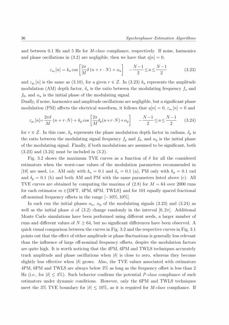
36 Synchrophasor Estimation Algorithms
and between 0.1 Hz and 5 Hz for M-class compliance, respectively. If noise, harmonics
and phase oscillations in (3.2) are negligible, then we have that η[n] = 0,
εar [n] = ka cos
[2π
Mδ (n+ r ·N) + αa
]−N−1
2≤n≤N−1
2(3.23)
and εpr [n] is the same as (3.10), for a given r ∈ Z. In (3.23) ka represents the amplitude
modulation (AM) depth factor, δa is the ratio between the modulating frequency fa and
f0, and αa is the initial phase of the modulating signal.
Dually, if noise, harmonics and amplitude oscillations are negligible, but a significant phase
modulation (PM) affects the electrical waveform, it follows that η[n] = 0, εar [n] = 0 and
εpr [n]=2πδ
M(n+ r·N) + kp cos
[2π
Mδp(n+r·N)+αp
]−N−1
2≤n≤N−1
2(3.24)
for r ∈ Z. In this case, kp represents the phase modulation depth factor in radians, δp is
the ratio between the modulating signal frequency fp and f0, and αp is the initial phase
of the modulating signal. Finally, if both modulations are assumed to be significant, both
(3.23) and (3.24) must be included in (3.2).
Fig. 3.2 shows the maximum TVE curves as a function of δ for all the considered
estimators when the worst-case values of the modulation parameters recommended in
[18] are used, i.e. AM only with ka = 0.1 and δa = 0.1 (a), PM only with kp = 0.1 rad
and δp = 0.1 (b) and both AM and PM with the same parameters listed above (c). All
TVE curves are obtained by computing the maxima of (2.8) for M = 64 over 2000 runs
for each estimator m ∈DFT, 4PM, 6PM, TWLS and for 101 equally spaced fractional
off-nominal frequency offsets in the range [−10%, 10%].
In each run the initial phases αa, αp of the modulating signals (3.23) and (3.24) as
well as the initial phase φ of (3.2) change randomly in the interval [0, 2π]. Additional
Monte Carlo simulations have been performed using different seeds, a larger number of
runs and different values of N ≥ 64, but no significant differences have been observed. A
quick visual comparison between the curves in Fig. 3.2 and the respective curves in Fig. 3.1
points out that the effect of either amplitude or phase fluctuations is generally less relevant
than the influence of large off-nominal frequency offsets, despite the modulation factors
are quite high. It is worth noticing that the 4PM, 6PM and TWLS techniques accurately
track amplitude and phase oscillations when |δ| is close to zero, whereas they become
slightly less effective when |δ| grows. Also, the TVE values associated with estimators
4PM, 6PM and TWLS are always below 3% as long as the frequency offset is less than 2
Hz (i.e., for |δ| ≤ 4%). Such behavior confirms the potential P-class compliance of such
estimators under dynamic conditions. However, only the 6PM and TWLS techniques
meet the 3% TVE boundary for |δ| ≤ 10%, as it is required for M-class compliance. If

Accuracy performance analysis 37
−10 −5 0 5 100
1
2
3
4
5
6
7
δ [%]
TV
E [
%]
6PM
4PM
DFT DFT
4PM
6PM
TWLS TWLS
(a)
−10 −5 0 5 100
2
4
6
8
δ [%]
TV
E [
%]
DFT
4PM
6PM6PM
4PM
DFT
TWLS TWLS
(b)
−10 −5 0 5 100
2
4
6
8
δ [%]
TV
E [%
]
DFT DFT
TWLS
6PM
4PM4PM
6PM
TWLS
(c)
Figure 3.2: Worst-case TVE patterns associated with different phasor estimators under the influence of
static off-nominal frequency offsets and sinusoidal amplitude modulation with ka = 0.1 and δa = 0.1
(a), off-nominal frequency offsets and sinusoidal phase modulation with kp = 0.1 rad and δp = 0.1 (b) or
both (c).

38 Synchrophasor Estimation Algorithms
Table 3.1: Maximum additional contribution to the TVE associated with different synchrophasor esti-
mators due to AM or/and PM. All modulation parameters are set equal to the worst-case conditions
recommended in the Standard IEEE C37.118.1-2011.
∆md DFT 4PM 6PM TWLS
AM 0.5% 0.3% 0.4% 0.08%
PM 0.8% 0.6% 0.6% 0.08%
AM+PM 0.9% 0.9% 0.9% 0.1%
we refer to ∆md , for d ∈ AM, PM, AM+PM, as the largest TVE increments due to
AM, PM or both, an upper-bound to the TVE in the presence of amplitude and/or phase
modulation is given by:
TVEmUBd
(δ) = TVEmmax(δ) + ∆m
d (3.25)
where the superscript m ∈DFT, 4PM, 6PM, TWLS refers to the chosen estimation
technique and TVEmmax results from (3.11)-(3.22), respectively. The values of ∆m
d are
summarized in Tab. 3.1 and are generally smaller than the TVE caused by the off-nominal
frequency offsets alone, provided that |δ| is large enough. The only exceptions refer to
the case of TWLS estimator, whose ∆md values become comparable to the maximum TVE
contributions due to the off-nominal frequency offsets alone, especially when both AM
and PM occur. In any case the sensitivity of all algorithms to PM oscillations is always
slightly larger than to AM fluctuations. The sensitivity of the four considered estimators
to the various modulation parameters has been analyzed by changing both the modulation
depth factor and the modulating frequency.
Fig. 3.3 shows the additional contributions to the maximum TVE values due to
PM, after compensating the influence of the off-nominal frequency offsets. The lines
in Fig. 3.3(a)-3.3(b) refer to different estimators and are plotted as a function of the
modulation factor kp, for δ = 0% and δ = 10%, respectively, after setting δp = 0.1 in
both cases.
Fig. 3.3(c)-3.3(d) shows the TVE increments due to PM as a function of δp, for δ = 0%
and δ = 10%, respectively, after setting kp= 0.1 rad. It is worth noticing that in most cases
the maximum TVE values grow roughly linearly with the modulation parameters. As
stated above, the 4PM and 6PM techniques effectively track the phasor variations around
the nominal frequency with increasingly better performance. However, their sensitivity to
PM degrades and become comparable to the DFT technique when |δ| grows. Therefore,
when δ is close to one of the extreme values recommended in the Standard (i.e. |δ| =10%), the 4PM and 6PM techniques outperform the DFT estimator mostly because of
their capability to mitigate the TVE growth caused by the off-nominal frequency offsets,

Accuracy performance analysis 39
0 0.02 0.04 0.06 0.08 0.10
0.2
0.4
0.6
0.8
kp
Ma
x T
VE
in
cre
me
nt
[%]
δ=0%
6PM
4PM
DFT
TWLS
(a)
0 0.02 0.04 0.06 0.08 0.10
0.2
0.4
0.6
0.8
kp
Max
TV
E in
crem
ent [%
]
δ=10%
6PM
4PMDFT
TWLS
(b)
0 0.02 0.04 0.06 0.08 0.10
0.2
0.4
0.6
0.8
δp
Ma
x T
VE
incr
em
en
t [%
]
δ=0%
6PM
4PM
DFT
TWLS
(c)
0 0.02 0.04 0.06 0.08 0.10
0.2
0.4
0.6
0.8
δp
Max
TV
E in
crem
ent [%
]δ=10%
6PM
4PM
DFT
TWLS
(d)
Figure 3.3: Worst-case TVE increments as a function of different PM parameters for δ = 0% (a)-(c) and
δ = 10% (b)-(d). In (a) and (b) δp = 0.1, while in (c) and (d) kp = 0.1.
regardless of the amount of amplitude or phase modulations.
On the contrary, the TWLS estimator is more insensitive than the others to PM, while
the influence of static frequency offsets and PM on the TVE are comparable. The results
of the TVE sensitivity analysis to the AM parameters are shown in Fig. 3.4. The meaning
of the curves and the values of the dual modulation parameters δa and ka is the same
as those in Fig. 3.3. The trend of the various patterns and the related considerations
are also quite similar. Even if the curves in Fig. 3.4(d) do not exhibit a linear behavior
any longer, the DFT, 4PM, 6PM and TWLS estimators (in this order) have increasingly
better performance in tracking possible AM fluctuations.
In addition, the AM sensitivity variations of each method are less affected by static off-
nominal offsets than in the PM case.

40 Synchrophasor Estimation Algorithms
0 0.02 0.04 0.06 0.08 0.10
0.1
0.2
0.3
0.4
0.5
ka
Max
TV
E in
crem
ent [%
]
δ=0%
6PM
4PM
DFT
TWLS
(a)
0 0.02 0.04 0.06 0.08 0.10
0.1
0.2
0.3
0.4
0.5
ka
Max
TV
E in
crem
ent [%
]
δ=10%
6PM
4PMDFT
TWLS
(b)
0 0.02 0.04 0.06 0.08 0.10
0.1
0.2
0.3
0.4
0.5
δa
Max
TV
E in
crem
ent [%
]
δ=0%
6PM
4PM
DFT
TWLS
(c)
0 0.02 0.04 0.06 0.08 0.10
0.1
0.2
0.3
0.4
0.5
δa
Max
TV
E in
crem
ent [%
]δ=10%
DFT
6PM
4PM
TWLS
(d)
Figure 3.4: Worst-case TVE increments as a function of different AM parameters for δ = 0% (a)-(c) and
δ = 10% (b)-(d). In (a) and (b) δa = 0.1, while in (c) and (d) ka = 0.1.
3.3.3 Effect of harmonics
In the previous section the effect of harmonics or wideband noise was assumed to be
negligible. In the following the influence of either disturbance is evaluated separately. In
terms of notation, the effect of harmonics in (3.2) can be modeled as
η[n]=H∑h=2
Xh ·cos
[2π
Mh(1 + δ)
(n+r ·+1
2
)+αh
]− N − 1
2≤n≤ N − 1
2(3.26)
for r ∈ Z. In (3.26) Ah and αh are the amplitude and the initial phase of the hth
harmonic for h = 1, . . . , H and H is the number of harmonics with a significant amplitude.
According to the Standard IEEE C37.118.1-2011, the first 50 harmonics should be taken
into account individually. In particular, a necessary condition for P-class or M-class
compliance is to assure that TV E ≤ 1% when the amplitude of each harmonic up to the
50th is either 1% or 10% of the fundamental component, respectively. In order to assess
the impact of harmonic distortion, several Monte Carlo simulations have been performed

Accuracy performance analysis 41
−10 −5 0 5 100
2
4
6
8
10
δ [%]
TV
E [
%]
DFTDFT
4PM
6PM6PM
4PM
TWLS TWLS
(a)
−10 −5 0 5 100
2
4
6
8
10
δ [%]
TV
E [
%]
6PM 6PM
4PM 4PM
DFTDFT
TWLS TWLS
(b)
Figure 3.5: Worst-case TVE patterns associated with different phasor estimators under the influence
of harmonics, static frequency offsets and sinusoidal amplitude and phase modulations with ka = 0.1,
δa = 0.1, kp = 0.1 rad and δp = 0.1. In (a) just the second-order harmonic is included, while in (b) all
harmonics till the 50th are considered. In both cases the amplitude of all harmonics is set equal to 1%
of the fundamental tone.
including AM and PM modulation, different static off-nominal frequency offsets in the
range [−10%, 10%] and one or multiple harmonics of relative amplitude equal to 1% of the
fundamental component. Each simulation consists of 2000 runs. Also M=128 samples per
cycle was used to avoid aliasing problems. In each run the initial phases of the modulating
signals, the fundamental tone and the harmonics change randomly in the interval [0, 2π].

42 Synchrophasor Estimation Algorithms
Fig. 3.5 shows the worst-case TVE patterns for every analyzed estimator when just only
the second harmonic or all harmonics till the 50th are considered, respectively. In all cases
the fundamental component is modulated both in amplitude and in phase with parameter
values equal to the maxima specified in the Standard C37.118.1-2011 (i.e. ka=0.1, δa=0.1,
kp=0.1 rad and δp=0.1). The corresponding upper bound to the TVE can be expressed
as
TVEmUBH,d
(δ) ∼= TVEmmax(δ) + ∆m
d +H∑h=1
∆mhd, (3.27)
where m ∈DFT, 4PM, 6PM, TWLS, d ∈AM, PM, AM+PM, TVEmmax(δ) results
from (3.11)-(3.22), the ∆md values are those described in 3.1, and the sum
∑Hh=1 ∆m
hd
represents the cumulative worst-case TVE increment due to the superimposition of H
harmonics. The individual contributions associated with the second-order and the third-
order harmonic (namely for h = 2, h = 3) when their relative amplitude is equal to
1% of the fundamental component are reported in Tab.3.2. As expected, the second-
order harmonic has the largest influence due to its minimal spectral distance from the
fundamental frequency. Observe that the TVE increments for h = 3 become negligible
when the 6PM or the TWLS techniques are used. No precise ∆m3d
values are reported in
this case because they are so small as to be comparable with the uncertainty due to the
finite number of simulation runs. Similarly, the values of ∆mhd
for h > 3 are not reported in
Tab.3.2, because they are negligible in all cases. In fact, when the off-nominal frequency
offset δ changes between [−10%, 10%], the harmonic frequencies do not fall any longer on
the zero-crossings of the discrete-time window Fourier transform (e.g. rectangular in all
cases except the TWLS) that multiplies the input data. As a result, the worst-case TVE
influence of the second- and third-order harmonics depends on how the magnitude of the
window spectrum side-lobes affect the considered estimator.
Fig. 3.5 shows also that the 6PM and TWLS techniques assure a maximum TVE value
lower than 1% under the joint effect of AM, PM and harmonics when |δ| ≥ 4%. However,
when harmonics with a relative amplitude up to 10% are considered (as it is required for
M-class compliance) the values of ∆mhd
(not reported here for the sake of brevity) become
about 1 order of magnitude larger than those in Tab. 3.2. Accordingly, the overall 1%
TVE limit specified in the Standard IEEE C37.118.1-2011 is exceeded and the M-class
compliance cannot be achieved by anyone of the considered estimators.
3.3.4 Effect of wideband noise
In order to analyze the impact of wideband noise on phasor estimator accuracy, further
Monte Carlo simulations have been performed assuming that η[n] is a white, Gaussian
noise sequence with a zero mean and a variable standard deviation. No harmonics and

Accuracy performance analysis 43
off-nominal offsets have been included in this new set of simulations. Again, the AM and
PM modulation parameters are equal to the maxima specified in the Standard C37.118.1-
2011 (i.e., ka = 0.1, δa = 0.1, kp = 0.1 rad and δp = 0.1) and M=128 samples per cycle
are acquired. However, the values of φ, αa and αp in (3.2), (3.23) and (3.24), respectively,
in this case do not change randomly. In fact, they are chosen in such a way that the
TVE values associated to the various estimators reach their respective maxima. Hence,
during simulations, the TVE contribution due to amplitude and phase modulations is
constant and equal to the maximum value reported in Fig. 3.2(c) for a certain value of
δ. In every simulation run, 1000 noise sequences of given variance have been added to a
waveform of known power. This procedure has been repeated for different signal-to-noise
ratio (SNR) values.
The TVE mean values and standard deviations related to the DFT, 4PM, 6PM and
TWLS techniques are plotted as a function of SNR for δ = 0% in Fig. 3.6, respectively.
Observe that when the SNR exceeds 40 dB, the effect of wideband noise is negligible. In
fact, the mean value patterns converge to the same results reported in Fig. 3.2 when δ =
0%. In addition, the TVE standard deviations for SNR ≥ 40 dB are in the order of 0.1%
or below. Quite interestingly, the standard deviation curves are almost independent of
the chosen estimation technique. Additional simulation results confirm that they are also
quite independent of the off-nominal frequency offset. It is worth noticing that the mean
values are significantly influenced by noise, only when the “native” TVE contribution
caused by off-nominal offsets and/or modulations is smaller than the TVE fluctuations
introduced by noise. Indeed, when the SNR is below a certain threshold, the additive
noise affecting the numerator of (2.8) may change the sign of the quantity ˆXmr − Xr. In
such cases, the TVE values are biased by the modulus operator in (2.8). When instead
the magnitude of the noise-related TVE fluctuations is not large enough to change the
sign of ˆXmr − Xr , the TVE bias due to noise is negligible.
In Fig. 3.6(a) this behavior is particularly evident for the DFT estimator. Indeed, the
Table 3.2: Maximum TVE increments of different synchrophasor estimators due to the second-order and
the third-order harmonics alone. The amplitude of both harmonics is set equal to 1% of the fundamental
component.
∆mhh
h=2 h=3
DFT 4PM 6PM TWLS DFT 4PM 6PM TWLS
AM 0.30% 0.20% 0.30% 0.20% 0.20% 0.10% < 0.1% < 0.1%
PM 0.30% 0.30% 0.30% 0.20% 0.20% 0.20% < 0.1% < 0.1%
AM+PM 0.30% 0.30% 0.30% 0.20% 0.20% 0.20% < 0.1% < 0.1%

44 Synchrophasor Estimation Algorithms
10 20 30 40 50 600
0.5
1
1.5
2
2.5
3
3.5
4
SNR [dB]
Me
an o
f T
VE
[%
]
DFT
6PM4PM
TWLS
(a)
10 20 30 40 50 600
0.5
1
1.5
2
2.5
3
3.5
4
SNR [dB]
Std
. D
ev.
of
TV
E [
%]
DFT
6PM4PM
TWLS
(b)
Figure 3.6: Mean (a) and standard deviation (b) values of the TVE associated with different phasor
estimators as a function of the SNR for δ = 0% and under the influence of sinusoidal amplitude and
phase modulations with ka = 0.1, δa = 0.1, kp = 0.1 rad and δp = 0.1. In all cases the initial phases of
both the fundamental component and the modulating signals are set so as to maximize the TVE.
TVE mean value curve tends to increase suddenly when the SNR is below 25 dB. The TVE
mean value curves associated with the others estimators instead start growing for larger
SNR values since their “native” TVE contribution due to modulations and/or off-nominal
frequency offsets is smaller. Notice that the growth rate of the TVE mean value curves is
larger than the growth rate of the respective standard deviation curves. Furthermore, if

Transient performance analysis 45
we just focus our attention on the increment in TVE as a function of the noise power (or
equivalently for decreasing SNR values) after removing the “native” TVE component, it
can be observed that the noise sensitivity of the DFT estimator is slightly lower than the
sensitivity of the 4PM, 6PM and TWLS techniques.
3.4 Transient performance analysis
In this section several simulations results are reported to compare the performance of
DFT, 4PM, 6PM and TWLS phasor estimators under the effect of various transient
disturbances. Specifically, the following cases are considered:
A. amplitude step changes both in nominal and off-nominal frequency conditions;
B. phase step changes both in nominal and off-nominal frequency conditions;
C. frequency linear ramps.
The values of all parameters modeling the transient phenomena described above are varied
within the boundaries specified in the Standard, while M=64 in all cases. For the sake of
clarity, different types of disturbances will be analyzed in different subsections. Generally,
the accuracy of phasor estimators is expressed in terms of TVE, which is defined as (2.8).
However, in some applications (e.g., when the maximum tolerable timing-related phase
error must be evaluated a priori [38]), the individual values of magnitude and phase
estimation errors can be more useful. In particular, such quantities are defined as:
ea =| ˆXm
r | − | Xr || Xr |
eb = ∠ ˆXmr − ∠Xr (3.28)
In the case of step variations the main performance parameters of interest are: the peak
values of TVE and (3.28), and the response time defined in section 2.2.2. In the Standard
the threshold to compute the response time is set equal to 1%. However, given that 1%
represents a cumulative upper bound for the whole PMU, a smaller threshold (e.g., 0.3%)
is advisable when just the estimation algorithm is considered. Thus, in the following,
the response time values related to both TVEmr = 1% and TVEm
r = 0.3% are reported.
Further simulations performed to estimate the delay time show that the values are always
in the order of 1-2 ms for all the considered estimators, i.e. negligible compared to the
latencies introduced by the input transducers and the front-end PMU circuitry. In the
case of linear frequency variations, the estimator performance is assessed in terms of
TVE as a function of the frequency rate of change of the collected waveform. Again,
the rate of change and the maximum frequency offset values are chosen in accordance
with the Standard.

46 Synchrophasor Estimation Algorithms
−6 −4 −2 0 2 4 6−2
−1
0
1
2
ea [%]
ep [
cra
d]
6PMDFT
TWLS 4PM
6PMTWLS
DFT4PM
Figure 3.7: Maximum and minimum envelopes of the phase estimation errors as a function of the relative
magnitude errors for 200 values of the waveform initial phase in [0, 2π]. In all cases, δ = 0% and ka = 10%.
3.4.1 Amplitude Step Change
If both an amplitude step and a possible static frequency offset affect (3.2), the functions
εa(t) and εp(t) are defined, respectively, as
εa(t) = kau(t− td) εp = 2πf0δt (3.29)
where ka is the relative size of the step with respect to amplitude A, u(t) is the unit step
function, td represents the time at which the step occurs and δ is the relative off-nominal
frequency offset. It is quite clear that, for a given value of ka, the effect of a step on the
estimated synchrophasor depends on when it occurs within a waveform cycle.
The curves in Fig. 3.7 show the maximum and the minimum envelopes of ep(·) (expressed
in crad) as a function of ea(·) (expressed in %) in nominal frequency conditions (i.e. for
δ = 0) and for ka = 10%. Such envelopes have been computed assuming that the step
occurs always at the same time, with the waveform initial phase changing linearly by
π/100 in [0, 2π]. Different line colors refer to different estimators, i.e. DFT (black line),
4PM (blue line), 6PM (green line) and TWLS (red line). Since the TVE is almost equal
to the quadrature sum of phase and magnitude errors [38], it is evident that in this case
the TVE values are dominated by the magnitude errors. Further simulation results (not
reported here for the sake of brevity) confirm that the magnitude error increment due to
an amplitude step of given size ka is approximately the same regardless of the value of δ.
The curves in Fig. 3.8 show the worst-case TVE values returned by the four considered
estimators as a function of ka in the range [−10%, 10%] and for δ = 0%, as suggested in
[18]. Observe that two curves are plotted for each estimator. In fact, they refer to the

Transient performance analysis 47
−10 −5 0 5 100
2
4
6
8
ka [%]
TV
E [
%]
TWLS
DFT
6PM
4PM
TWLS
6PM
DFT
4PM
Figure 3.8: Maximum and minimum worst-case TVE patterns as a function of the relative step magnitude
ka. All patterns are obtained by changing the waveform initial phase values and the moment when the
step occurs in a cycle.
minimum and maximum worst-case TVE values obtained by changing both td and φ .
Note also that the TVE grows almost linearly with |ka| and that the behavior of the four
estimators is very similar. Since the upper-bound to the TVE in the presence of both
off-nominal frequency offsets and amplitude modulation is approximately given by the
sum of both contributions [40], a similar behavior holds even when an amplitude step is
considered. Indeed, by extrapolating the results of Fig. 3.8, it can be easily shown that
TVEmapeak
(ka, δ) ≈
ba1ka + TVEmoffδ ka ≥ 0
ba2ka + TVEmoffδ ka < 0
(3.30)
where m ∈DFT, 4PM, 6PM,TWLS and TVEmoff (δ) is the maximum TVE contribution
caused by the off-nominal frequency offset δ [40].
Coefficients ba1 = 0.51 ± 0.06 and ba2 = −0.58 ± 0.07 represent the TVE growth rates
caused by the step in nominal frequency conditions (i.e., when δ = 0). Consider that the
uncertainty associated with both coefficients is due to both the chosen estimator and the
phase of the signal when the step occurs.
Fig. 3.9 displays the worst-case response time values expressed in nominal waveform
cycles, as a function of ka in the range [−10%, 10%] for δ = 0% and δ = 4% and for
two different TVE thresholds, i.e. 1% and 0.3%, respectively. All curves have been
obtained by changing the time at which the step occurs within a full waveform cycle and
by computing the maximum response times for the same value of ka. The evident curve
asymmetry visible in Fig. 3.9(b) and 3.9(d) is due to the positive off-nominal frequency

48 Synchrophasor Estimation Algorithms
−10 −5 0 5 100
0.5
1
1.5
ka [%]
resp
onse
tim
e [c
ycle
]
δ=0%
TWLS
4PM
6PM
DFT
6PM
TWLS
DFT
4PM
(a)
−10 −5 0 5 100
0.5
1
1.5
ka [%]
resp
onse
tim
e [c
ycle
]
δ=4%
4PM
6PM6PM
4PM
TWLSTWLS
(b)
−10 −5 0 5 100
0.5
1
1.5
2
2.5
3
ka [%]
resp
onse
tim
e [c
ycle
]
δ=0%
6PM
DFT
TWLS
4PM
6PM
DFT
4PM
TWLS
(c)
−10 −5 0 5 100
0.5
1
1.5
2
2.5
3
ka [%]
resp
onse
tim
e [c
ycle
]δ=4%
6PM6PM
TWLS TWLS
(d)
Figure 3.9: Worst-case response time values expressed in nominal waveform cycles as a function of the
amplitude step size ka for TVE=1% and δ = 0% (a), TVE=1% and δ = 4% (b), TVE=0.3% and δ = 0%
(c), TVE=0.3% and δ = 4% (d). Curves are missing when the response time of the related estimator is
undefined. This happens in (b) and (d) when the static off-nominal TVE is larger than the 1% or 0.3%
threshold.
offset. The discontinuous behavior observable in some of the curves is due to the fact that
the TVE patterns associated with some phasor estimators exhibit multiple and irregular
ripples of decreasing amplitude in the time domain, as shown in Fig. 3.10. The reported
TVE patterns have been obtained using a step of relative size ka = 5% for δ = 0% in
(a) and δ = 4% in (b), respectively. In both cases φ = 0. Of course, when the step
size increases, the ripple amplitude grows accordingly. As a consequence, the 1% or 0.3%
TVE thresholds are suddenly and progressively crossed by multiple ripples, especially if
the 6PM technique is used. An analytical expression describing the TVE pattern as a
function of time when a one-cycle DFT phasor estimator is applied to a waveform of
nominal frequency (i.e. with δ = 0%) is reported in the following.
Proof of expression of amplitude or phase steps effect on DFT estimators. Let us assume

Transient performance analysis 49
0 0.05 0.1 0.15 0.20
1
2
3
4
5
time [s]
TV
E [
%]
δ=0%
TWLS
DFT
6PM4PM
(a)
0 0.05 0.1 0.15 0.20
1
2
3
4
5
time [s]
TV
E [
%]
δ=4%
DFT
4PM6PMTWLS
(b)
Figure 3.10: TVE patterns as a function of time for δ = 0% (a) and δ = 4% (b), assuming that a step of
relative size ka = 5% occurs after 0.1 s the time reference.
that an ideal electric sine wave of nominal frequency f0 (i.e. with δ=0%) is affected by an
amplitude or a phase step described by (3.29) or (3.35), respectively, at time td = d/fs.
Since steps do not change waveform frequency, when t ≥ td x(t) can be easily rearranged
as a sum of two sine waves of frequency f0, i.e.
x(t) = X1cos[2πf0t+ φ] +X2 cos[2πf0t+ γ] (3.31)
where X1 = A, X2 = ka · A, and γ = φ if an amplitude step occurs, or X1 = A · cos kp,
X2 = A · sin kp, and γ = φ+ π2
when a phase step is applied. As a result, the phasor at a

50 Synchrophasor Estimation Algorithms
generic reference time tr = r/fs with r ∈ Z is given by
Xr =
A√2· ejϕr r < d
X1√2· ejϕr + X2√
2· ejγr r > d
(3.32)
where ϕr is defined as in (2.4), while γr = ϕr or γr = ϕr + π2
depending on whether an
amplitude or a phase step occurs. Suppose that the samples of (3.31) are collected by a
PMU in ideal conditions (without considering noise or disturbances) and that (3.3), with
N = M , is used to estimate (3.32). Since waveform sampling and acquisition is perfectly
coherent (i.e., f0 = M · fs), if the DFT observation interval does not include the step, no
magnitude or phase errors affect the estimation result. On the contrary, when the step
occurs within an observation interval, the estimation errors depend on how many samples
are collected before d and r. From these simple considerations, it can be easily shown that
TVEDFTr =
0 r < d− M−12
+ s| ˆXDFTr − A√
2·ejϕr |
| A√2·ejϕr | d− M−1
2+ s 6 r < d
| ˆXDFTr −X1√
2·ejϕr−X2√
2·ejγr |
|X1√2·ejϕr X2√
2·ejγr |
d ≤ r 6 d+ M−12− s
0 r ≥ d+ M−12− s
(3.33)
where s=0 or 1/2 depending on whether M is an odd or an even number, respectively,
and ˆXDFTr is the phasor estimated by (3.3). In particular after several algebraic steps, it
can be proved that
ˆXDFTr =
1
M√
2(A · Er +X1 · Fr +X2 ·Gr) (3.34)
where
Er = (d− r + M−12
)ejϕr +sin[ 2πM (d−r+M−1
2 )]sin( 2π
M )e−j[
2πM (M+1
2−d−)φ]
Fr = (r + M−12− d)ejϕr +
sin[ 2πM (r+M−12−d)]
sin( 2πM )
e−j[2πM (M+1
2+d)+φ]
Gr = (r + M−12− d)ejγr +
sin[ 2πM (r+M−12−d)]
sin( 2πM )
e−j[2πM (M+1
2+d)+γ].
Observe that, in accordance with (3.32), the leftmost terms of Er, Fr and Gr in (3.4.1) are
responsible for the almost triangular TVE pattern behavior visible in Fig. 3.10(a). The
rightmost terms in (3.4.1) instead cause TVE oscillations and ripples whose size depends
on the relationship between φ and d. In the case of the DFT phasor estimator, such
terms are very small, so they do not affect the response times significantly. However, in
the other estimators (e.g. 6PM), they can be much larger.

Transient performance analysis 51
−10 −5 0 5 100
2
4
6
8
10
kp [degree]
TV
E [%
]
TWLS
6PM
4PM
DFT
4PM
6PM
DFT
TWLS
Figure 3.11: Maximum and minimum worst-case TVE patterns as a function of the relative step magni-
tude kp. All patterns are obtained by changing the waveform initial phase values and the moment when
the step occurs in a cycle.
The agreement between this expression and corresponding simulation results reported
in Fig. 3.10(a) is excellent. Similar expressions could be also derived for the other analyzed
estimators. Observe that some response time curves (namely those associated with the
DFT phasor estimator in off-nominal conditions and the 4PM estimator for δ = 4% and
TVE= 0.3%) are missing. In such cases the TVE patterns are never steadily below the
target threshold. Therefore, the response times are undefined. In all the other cases, the
response time values are below the boundaries reported in [18] (i.e., 1.7/f0 = 0.034 s for
P-class and M-class PMUs at the maximum reporting rate) when the TVE threshold is
set to 1%. When the threshold is lowered to 0.3%, the response times generally tend to
grow and become more sensitive to possible off-nominal frequency offsets. However, the
TWLS technique is quite robust. Observe that, in all cases, when |ka| is small enough,
the response times are zero, because the maximum TVE values are always smaller than
the given threshold.
3.4.2 Phase Step Change
If a step affects the phase of waveform (3.2), but no significant amplitude variations occur,
the functions εa(t) and εp(t) can be expressed as
εa(t) = 0 and εp(t) = 2πf0δt+ kpu(t− td). (3.35)
The worst-case TVE curves related to the four considered estimators as a function of kpin the range [−10, 10] are shown in Fig. 3.11 for δ = 0%. Similarly to what is reported

52 Synchrophasor Estimation Algorithms
in Fig. 3.8 all TVE patterns exhibit similar values and grow linearly with |kp|. Therefore,
also in this case the maximum TVE values caused by possible out-of-range phase steps
can be easily extrapolated by means of the following expression
TVEmppeak
= (kp, δ) ≈ bp|kp|+ TVEmoff (δ), (3.36)
where m ∈ DFT, 4PM, 6PM, TWLS, bp = 0.93± 0.09 is the TVE growth rate caused
by the phase step when δ=0%, and the meaning of TVEmoff (δ) is the same as in Section
3.3.1.Consider that if kp is expressed in crad rather than in degrees, then bp = 0.53±0.05.
Therefore, the TVE sensitivity of all estimators to amplitude and phase steps is quite
similar. Observe also that the uncertainty associated to the TVE growth rate depends
on the phase of the waveform when the step occurs, as well as on the properties of the
considered estimator. Nonetheless, the step-related TVE increments are quite similar for
all techniques, regardless of the value of δ. Moreover, they are almost symmetric with
respect to kp and they are dominated by the phase error contribution. In Fig. 3.12 the
worst-case response time curves are plotted as a function of kp in the range [−10, 10], for
δ = 0% and δ = 4% and for two different TVE thresholds, i.e. 1% and 0.3%, respectively.
Response time values have been obtained by changing linearly the time at which the step
occurs within a full waveform cycle and are expressed in waveform cycles at the nominal
frequency. Different line color refer to different estimators, in accordance with the notation
already used. The considerations about the curves in Fig. 3.12 are the same as those in
Fig. 3.9. However, in this case the maximum response time of the 6PM technique exceeds
the 1.7/f0 limit reported in [18] when |kp| > 8. Again some DFT and 4PM curves
are missing in Fig. 3.12(b)- 3.12(d) because the TVE is never steadily below the chosen
threshold. Quite interestingly, the TWLS method exhibits excellent performance (smaller
than 1 cycle) when the TVE threshold is set to 1%, even if the observation interval is
about four cycles long. However, when the TVE threshold is set to 0.3%, the response
time may become much longer. It is also worth noticing that the responsiveness of the
TWLS method is very insensitive to δ. This is due to the very good performance of this
estimator in tackling possible static frequency offsets.
3.4.3 Linear Frequency Ramp
If the frequency of the electrical waveform (3.2) is subjected to a linear variation and no
amplitude changes occur, then εa and εp can be expressed as
εa(t) = 0 and εp = πRf t2 (3.37)
where Rf represents the frequency rate expressed in Hz/s.

Transient performance analysis 53
−10 −5 0 5 100
0.5
1
1.5
2
2.5
kp [degree]
resp
on
se tim
e [cy
cle
]
δ=0%
6PM6PM
DFTTWLS TWLS
DFT
4PM 4PM
(a)
−10 −5 0 5 100
0.5
1
1.5
2
2.5
kp [degree]
resp
on
se tim
e [cy
cle
]
δ=4%
4PMTWLS
6PM
4PMTWLS
6PM
(b)
−10 −5 0 5 100
0.5
1
1.5
2
2.5
3
kp [degree]
resp
on
se tim
e [cy
cle
]
δ=0%
6PM
TWLS
4PM
DFT DFT
4PM
TWLS
6PM
(c)
−10 −5 0 5 100
0.5
1
1.5
2
2.5
3
kp [degree]
resp
on
se tim
e [cy
cle
]
δ=4%
TWLS
6PM
TWLS
6PM
(d)
Figure 3.12: Worst-case response time values expressed in nominal cycles as a function of the phase step
size kp for TVE=1% and δ=0% (a), TVE=1% and δ=4% (b), TVE= 0.3% and δ=0% (c), TVE= 0.3%
and δ= 4% (d). Curves are missing when the response time is undefined. This happens when the TVE
is larger (or smaller) than 1% or 0.3%, for any value of kp.
In Fig. 3.13 the upper TVE envelopes associated with the one-cycle DFT, the 4PM,
the 6PM and the TWLS estimators, are plotted as a function of time over an interval of 5
s. In all cases the frequency rate is set equal to the upper bound specified in the Standard,
namely 1 Hz/s [18]. Clearly, the TVE grows with time, as expected. However, while the
TVE increment related to the TWLS estimator is basically negligible, one-cycle DFT,
4PM and 6PM violate the 1%. Clearly, the TVE grows with time, as expected. However,
while the TVE increment related to the TWLS estimator is basically negligible, one-cycle
DFT, 4PM and 6PM violate the 1% constraint recommended in the Standard after about
1 s, 3 s and 4 s, respectively. It is worth noticing that the relative frequency increment
during a single waveform cycle is very small. In fact, the relative off-nominal frequency
offset accumulated in a single waveform cycle when Rf = 1 Hz/s is just 4·10−4. Therefore,
the frequency changes can be regarded as quasi-static and the ramp can be reasonably

54 Synchrophasor Estimation Algorithms
0 1 2 3 4 50
1
2
3
4
5
6
7
time [s]
TV
E [%
]
6PM
4PM
DFT
TWLS
Figure 3.13: Maximum TVE envelopes in the presence of a linear frequency ramp growing with a rate of
1 Hz/s.
approximated by a staircase function built by accumulating small, frequency steps in
successive observation intervals. This interpretation explains why the TVE envelopes
shown in Fig. 3.13 are very close to the worst-case TVE curves reported as a function
of δ in [40] and why the TWLS technique exhibits the best performance. Indeed, this
estimator is excellent in static off-nominal conditions.
3.5 Conclusion
In this chapter after a presentation of state-of-art estimators, the performances of three
selected synchrophasor estimators are analyzed and compared with the classic one-cycle
DFT. The proposed analysis is divided in two parts.
In Section 3.3 the effect of static off-nominal frequency offsets, amplitude and phase
oscillations, harmonics and noise is evaluated. We purposely took into account such phe-
nomena in order to assess their impact on the estimator accuracy even in complex sce-
narios, i.e. when the electrical waveforms are affected by both quasi-stationary changes
and fast fluctuations. The reported simulation results and the corresponding analytical or
numerical upper bound expressions show that the 4PM and the 6PM techniques (which
track the time-varying synchrophasor behavior by estimating its first- and second-order
derivatives over subsequent non-overlapped observation intervals) have a moderate com-
plexity and can be compliant with the P-class accuracy requirements of the Standard
IEEE C37.118.1-2011, both under steady-steady and dynamic conditions, provided that
the SNR is large enough. However, neither one can assure M-class accuracy compliance

Conclusion 55
at a reporting rate equal to or larger than 50 sample/s, since the TVE boundaries are
violated in static conditions when the off-nominal frequency offset is about ±10%. The
Taylor Weighted Least Squares (TWLS) phasor estimators generally assure better accu-
racy in all conditions, especially if a window is used to weigh the samples of the collected
data records. However, also in this case the M-class accuracy compliance can be hardly
achieved when four waveform cycles are used. Further analysis to evaluate the accuracy
of these synchrophasor estimators in presence of out-of-band interferers show that all of
them are sensitive and not compliant with the Standard limits.
In Section 3.4 the performances of the same estimators have been analyzed in some
meaningful transient conditions described in the Standard IEEE C37.118.1-2011. The
classic one-cycle DFT technique has been also included as a reference. The reported
simulation results show that the TWLS approach is preferable in almost all conditions,
in spite of a longer observation interval. In the presence of amplitude or phase steps,
its response time is very insensitive to off-nominal frequency offsets and it is shorter
than one nominal waveform cycle, when the TVE threshold is set to 1%. The peak
TVE values of all estimators during step transients are generally comparable and can
be so high as a few percent. Therefore, no significant differences exist between such
techniques in terms of estimation accuracy. In the case of linear frequency ramps based
on the parameters reported in the Standard, all estimators work in quasi-static conditions.
Therefore, responsiveness is not an issue and accuracy is the same as under the effect of
static frequency offsets. Again, the TWLS estimator outperforms the other techniques.
Indeed, it is the only one to meet the 1% TVE limit during the transient in worst-
case conditions.

56 Synchrophasor Estimation Algorithms

Chapter 4
A Dynamic DFT-based
Synchrophasor Estimator
In this chapter, a novel algorithm for synchrophasor, frequency and ROCOF estimation
is defined and analyzed in depth. The proposed algorithm has been preliminary pre-
sented in [41]. At first the theoretical analysis underlying the new algorithm is presented.
Afterwards, the estimation accuracy and the algorithm performances are thoroughly an-
alyzed through simulations under different steady-state and transient testing conditions
described in the Standard IEEE C37.118.1-2011. The simulation results are a subset of
those reported in [41], since only the phasor estimation accuracy is considered in this
dissertation. Moreover, the performances of the same algorithm for phasor angle estima-
tion only are analyzed in depth. This could be particularly useful at the distribution level
where angle measurement accuracy ha to be much higher than at the transmission level.
4.1 Interpolated Dynamic DFT IpD2FT estimator
Let xr[n] be the real part of the electrical waveform acquired by a PMU as presented in
(2.3),i.e.
xr[n] = ReA[1 + εa(tr + nTs)] · ej[2πfx(tr+nTs)+φ]= Re
√2pr[n]ej
2πM
(1+δ)n (4.1)
where the operator Re· extracts the real part of its argument, A is the waveform
amplitude, Ts = 1/fs is the nominal sampling period, φ is the waveform initial phase
Part of this chapter was published in
G. Barchi, D. Fontanelli, D. Macii and D. Petri, “On the Accuracy of Phasor Angle Measurements in Power
Networks”, on IEEE Trans. Instr. and Meas.,vol.64, no., pp., 2015.

58 A Dynamic DFT-based Synchrophasor Estimator
and εa(·) and εp(·) are the intrinsic amplitude and phase fluctuations, respectively. Note
that in (4.1), the expression pr[n] denotes the waveform phasor referred to frequency
fx = f0(1 + δ) at a generic sampling time tr +n · Ts already introduced in (2.4). This can
be rewritten as:
pr[n] =A√2
[1 + εa(tr + nTs)] ej[2πf0(1+δ)tr+εp(tr+nTs)+φ]
=A√2
[1 + εar [n]] · ej[2πf0(1+δ)+εpr [n]+φ] (4.2)
As explained in Chapter 3, when a waveform phasor changes rapidly within the same
observation interval, the static phasor model is no longer adequate for estimation purposes.
In this situation, the waveform synchrophasor p′r[n] can be better described by its Taylor’s
series expansion around time tr truncated to the kth order term. As a result, (4.1) can
be rewritten as
xr[n] ∼=√
2
2
K∑k=0
(nkpr,ke
j 2πM
(1+δ)n + nkp∗r,ke−j 2π
M(1+δ)n
)(4.3)
where pr,k = 1K!p
(k)r (tr) · T ks , and p
(k)r (tr) is the kth order derivative of (4.2) computed at
time tr and the superscript ” ∗ ” denote the conjugate operator. It is worth noticing that
a digitized waveform processed by a PMU includes various disturbances. Therefore, it is
not expressed by (4.1), but rather by
sr[n] = xr[n] + εhr [n] + εnr [n] (4.4)
where εhr [·] includes all unwanted narrowband components (e.g. the first H harmonics
along with other possible out-of-band interferers), and εnr [·] is the additive wideband
noise. Assuming that in (4.4) both narrowband and wideband disturbances are negligible
(i.e. εhr [·] ≈ εnr [·] ≈ 0), if the windowed discrete-time Fourier transform is applied to
(4.3), it follows that [42], [19]:
Swr(λ) ∼= Xwr(λ) ∼=√
2
N
N−12∑
n=−N−12
xr[n]w[n]e−j2πNλn
∼=K∑k=0
pr,kWk(λ− ν) + p∗r,kWk(λ+ ν) (4.5)
where the real variable λ denotes the frequency expressed in bins, ν=fx·N·Ts= (1+δ)·N/Mis the fundamental frequency of (4.1) also expressed in bins,
W0(λ) =1
N
N−12∑
n=−N−12
w[n]e−j2πNλn (4.6)

Interpolated Dynamic DFT IpD2FT estimator 59
is the normalized discrete-time Fourier transform of the adopted window w[·] and
Wk(λ) =1
N
N−12∑
n=−N−12
nkw[n]e−j2πNλn =
(jN
2π
k) dkW (λ)
dλk(4.7)
(with k > 0) is a continuous function proportional to its derivative of order k. Consider
that in (4.5) ν can be also more conveniently expressed as C + ξ, where C = [N/M ]
represent the nominal (integer) number of observed cycles,
ξ =
C · δ if C ·M is odd
C · δ + 1+δM
if C ·M is even(4.8)
Indeed, if C ·M is an even number, an additional sample is required in order to process
records consisting of an odd number of samples. If the phasor Taylor’s series is truncated
to the second order (i.e., K = 2) and the chosen window exhibits an even symmetry with
respect to its central sample, the values of (4.5) for λ = C + h, h = 1, 0,−1, can be
rearranged as follows [41]
Swr∼= WP (ξ) · Pr +WI(ξ) · P ∗r (4.9)
where
Swr =
Swr(C − 1)
Swr(C)
Swr(C + 1)
Pr =
pr0
pr1
pr2
P ∗r =
p∗r0
p∗r1
p∗r2
(4.10)
and matrices
WP (ξ) =
W0(−1− ξ) W1(−1− ξ) W2(−1− ξ)W0(−ξ) W1(−ξ) W2(−ξ)W0(1− ξ) W1(1− ξ) W2(1− ξ)
(4.11)
WI(ξ) =
W0(2C − 1 + ξ) W1(2C − 1 + ξ) W2(2C − 1 + ξ)
W0(2C + ξ) W1(2C + ξ) W2(2C + ξ)
W0(2C + 1 + ξ) W1(2C + 1 + ξ) W2(2C + 1 + ξ)
(4.12)
consist just of real elements. If ξ is known, the real and the imaginary parts of vector Prare given by
RePr = [WP (ξ) +WI(ξ)]−1 ·ReSwr
ImPr = [WP (ξ)−WI(ξ)]−1 · ImSwr
(4.13)

60 A Dynamic DFT-based Synchrophasor Estimator
In particular, by denoting the solution of (4.13) with Pr = [pr0 , pr1 , pr2 ]T the synchrophasor
estimate at the reference time tr is simply pr0 . If ξ is unknown instead (which is the most
common case), the values of Pr can be obtained iteratively as follows. At first, ξ in (4.11)
and (4.12) is assumed to be equal to 0. Then, (4.13) is computed and the value of ξ is
obtained from (4.8), once the fractional frequency deviation δ is estimated from
δ(tr) =M
2π
Impr1 p∗r0|pr0|2
(4.14)
The new value of ξ is then replaced into (4.13) and the same procedure is repeated till
when the results of (4.14) do not change significantly. The algorithm flow chart is shown
in Fig. 4.1. Indeed the convergence of the algorithm, which relies on a gradient-based
approach (similarly to the classic Newton-Raphson method) is always guaranteed. In
the following, the algorithm expressed by (4.5)-(4.14) will be referred to as Interpolated
Dynamic DFT-based (IpD2FT) synchrophasor estimator [41].
Compute
Estimated frequency deviation
Initialize
Compute Does result change
significantly?
NO
EstimatedSynchrophasor
YES
Figure 4.1: Flow chart of the Interpolated Dynamic Discrete Fourier Transform (IpD2FT) algorithm.

Computational Complexity 61
4.2 Computational Complexity
As known, the evaluation of one DFT sample requires N complex products and N -1
complex additions. Therefore, complexity is O(N), i.e. proportional to the number of
collected samples. The complexity of the IpD2FT algorithm is still linear with N , but it
is larger than both DFT and TWLS estimators for various reasons, i.e.
• at least K+1 DFT samples of the transform of the acquired waveform have to be
computed;
• 2(K + 1)2 samples of the window spectrum have to be evaluated to build matrices
(4.11) and (4.12) ;
• such matrices have to be inverted;
• the algorithm is repeated L times;
• finally at the end of each iteration a new value of ξ has to be estimated using (4.14)
and (4.8).
Evidently, the computational cost of the last operations for obtaining ξ is negligible
compared with the rest of the algorithm. Therefore, assuming that the number of it-
erations L is fixed, the order of complexity of the IpD2FT estimator is approximately
O((K+ 1)·N) + 2L·[O((K+ 1)2·N) +O((K+ 1)3)], where the cubic rightmost term refers
to the complexity of inverting a (K+1)×(K+1) matrix, using the Gauss–Jordan elimina-
tion technique. Even if the overall complexity of the IpD2FT looks quite larger than the
other solutions, in practice the values of both K and L are small (e.g. K=2 and L=3).
Thus, the overall processing time to return a single phasor estimate is still dominated by
the number of samples N , and it is just slightly higher than using a basic DFT estimator.
4.3 Simulation results
In order to analyze the performance of the proposed algorithm, multiple Monte Carlo
simulations have been performed, considering fs=6.45 kHz (i.e. M = 129) and different
observation intervals, i.e. C=2, C=3, C=4 and C=6. The classic B-term cosine-class
window functions given by [43]:
w[n] =B−1∑b=0
ab cos
(2π
Nbn
)n = −(N − 1)
2, · · · , (N − 1)
2(4.15)
have been used. Of course the coefficients ab, with b=0,...,B-1, depend on the specific
window chosen since their spectra exhibit complementary performances. In particular
two types of windows are considered in the following: the Minimum Side-Lobe Level
(MSL) and the Maximum Side-Lobe level Decay (MSD) windows.

62 A Dynamic DFT-based Synchrophasor Estimator
−10 −5 0 5 100
0.02
0.04
0.06
0.08
0.1
0.12
0.14
0.16
δ [%]
max
(TV
E)
[%]
2T−MSL
3T−MSD
3T−MSL
2T−MSD
Figure 4.2: Maximum TVE values as a function of the off-nominal frequency deviations and joint effect
of amplitude and phase modulations with C=3, K=2 and different windows, i.e. 2- and 3-term MSD, 2-
and 3-term MSL [41].
4.3.1 Accuracy performance analysis
The accuracy performance of the IpD2FT estimator has been evaluated in different sce-
narios recommended by the Standard.
Fig. 4.2 shows the maximum values of TVE obtained after three iterations using 2-
term and 3-term MSL and MSD windows, respectively over a 3-cycle observation interval
(namely with C= 3 and N = 387). The worst-case TVE values are plotted as a function
of δ in the range [−0.1, 0.1] under the effects of amplitude modulation (AM) and phase
modulation (PM), but without any other disturbances (i.e. εhr [·] and εnr [·]). Amplitude
and phase of the modulating sine waves εa(t) and εp(t) are fixed and equal to the worst-
case values reported in the Standard, i.e. 0.1·A and 0.1·f0 in the case of AM, and 0.1 rad
and 0.1·f0 for PM, respectively. The initial phases of both the fundamental component
and the modulated signals are chosen randomly in [0, 2π] and the maxima result from 300
runs.
Table 4.1 reports the maximum normalized values of TVE for four different observation
interval length (i.e. C=2, C=3 , C=4 and C=6 ) and for different types of windows. In
order to better highlight the potential compliance with the requirements of the Standard,
the values reported in the Table are normalized by the respective threshold values TVEth.
Such thresholds refer to the case of M-class PMUs with a reporting rate RR/20 fps. The
values that exceed the Standard requirements are shadowed, in this way they are easily

Simulation results 63
identified in the Table.
In all cases the synchrophasor Taylor’s series is truncated to the second-order term
(i.e. K = 2). Some simulation have been performed assuming K = 3 and changing
(4.10)–(4.13) accordingly. However even if the robustness of the algorithm increases in
present of fluctuations, it becomes more sensitive to other disturbances (i.e. harmonics
and wide-band noise). So K=2 guarantees globally better performance. The considered
test conditions summarized below:
a) influence of a static relative frequency deviation δ alone, changing linearly in the
range |δ|≤ 0.1, in compliance with the worts-case requirements of the Standard
IEEE C37.118.1-2011;
b) sine-wave with static frequency deviation δ, like in case a, affected by zero-mean
additive wideband Gaussian noise with variance corresponding to a Signal-to-Noise
Ratio (SNR) of 60 dB. Since this case is not considered in the Standard, the threshold
is the same as in case a;
c) sine-wave affected by a static relative frequency deviation in the range |δ|≤ 0.1 and
by a second-order harmonic with magnitude equal to 10% of the fundamental tone;
d) similar to case c, but considering just the third-order harmonic with magnitude
equal to 10% of the fundamental tone;
e) AM waveform with a carrier fundamental frequency affected by an off-nominal rel-
ative deviation |δ|≤ 0.1 and with amplitude and frequency of the modulating signal
equal to 0.1·A and 0.1·f0, respectively;
f) AM+PM waveform with the carrier fundamental frequency affected by an off-nominal
relative deviation |δ|≤ 0.1 and with AM and PM modulating frequencies and am-
plitude equal to 0.1 · f0 and 0.1 · A (for AM) and 0.1 rad (for PM), respectively;
g) sine-wave at nominal frequency perturbed by an out-of-band sinusoidal interferer
with magnitude equal to 10% of the fundamental, phase chosen randomly in [0, 2π)
and frequency no smaller than 10 Hz, no larger than 2f0 and lying outside the
interval (f0–RR/2, f0 +RR/2) when RR = 50 fps.
The results reported in Tab. 4.1 lead to the following conclusions.
In case a, the estimation error, due mainly to the spectral leakage of the waveform
image component and by the Taylor’s series approximation error, is negligible compared
with the threshold specified in the Standard.
In case b the combined effect of frequency deviation and wide-band Gaussian noise
does not affect the TVE index.
In case c, the presence of 2nd-order harmonic when C=2 and C=3 may cause large
TVE values, i.e. the well beyond compliance thresholds. Indeed, the discrete-time Fourier

64 A Dynamic DFT-based Synchrophasor Estimator
Tab
le4.1:
Max
imu
mT
VE
norm
alizedby
thresh
oldT
VEth
(i.e.T
VE
/T
VEth
)va
lues
obtain
edu
sing
the
IpD
2FT
-based
estimator
with
the
Tay
lor’sseries
trun
cated
toord
erK
=2
and
with
diff
erentB
-termM
SL
an
dM
SD
win
dow
sover
2-3-
4-an
d6-cy
clein
tervals,resp
ectively[41].
Case
Test
conditio
ns
TVEth
C=
2–M
SL
C=3–M
SL
C=4–M
SL
C=6–M
SD
B=2
B=3
B=4
B=2
B=3
B=4
B=2
B=3
B=4
B=2
B=3
B=4
aF
req.
dev
.only
(±10%
)1
00
0.0
20
00
00
00
00
bF
req.
dev
.+noise
(60
dB
)bia
s1
00
00
00
00
00
00
std.
10.0
20.0
20.0
20.0
10.0
10.0
10.0
10.0
10.0
10.0
10.0
10.0
1
cF
req.
dev
.+2nd
harm
(10%
)1
6.6
8.2
11
1.3
3.3
4.7
0.1
20.5
1.4
0.0
60.0
20.0
4
dF
req.
dev
.+3rd
harm
(10%
)1
0.1
30.2
11.2
0.1
30.0
10
0.1
0.0
10
0.0
10
0
eF
req.
dev
.+A
M3
0.0
30.0
30.1
40.0
40.0
10.0
10.0
60.0
30.0
20.1
60.0
80.0
5
fF
req.
dev
.+A
M+
PM
30.0
30.0
30.1
50.0
50.0
10.0
10.0
80.0
40.0
30.2
60.1
20.0
7
gO
ut-o
f-band
interferen
ceonly
1.3
7.1
27.7
98.8
15.2
15.9
86.4
92.5
53.9
64.8
70.0
41.3
82.6
4

Simulation results 65
transform of a multi-frequency signal results from the superposition of the window spec-
trum replicas centered at different tones. If B is equal to or greater than C-1 (as it
happens in Tab. 4.1), the vector Xwr is heavily affected by the contribution of the sec-
ond harmonic, which interferes through the window spectrum main-lobe, thus heavily
perturbing the estimation result. Moreover, the amount of interference grows when B
increases, because the window spectrum main-lobe becomes wider. On the other hand,
when B is smaller than C-1, the interference caused by the harmonics is due to the spec-
trum side-lobes of the chosen window. Thus, as the difference between C and B grows,
the estimation accuracy improves.
Similar considerations hold in case d, even though the third-order harmonics are less
critical than the second-order ones, because the corresponding spectrum main-lobes are
farther apart from the fundamental. Higher-order harmonics are not considered because
they are filtered by the adopted windows.
The effect of amplitude and phase fluctuations, in case e and f is more relevant over
longer observation intervals, regardless of the chosen window. This behavior, which is
opposite to what happens in presence of off-nominal frequency deviations and harmonics,
suggests that a trade-off is necessary in order to fulfill all the Standard requirements.
Finally, in case g the values in Tab.4.1 show that out-of-band interfering tones inter-
harmonics generally cause large errors.. However, this effect can be mitigated by using
windows with a smaller number of terms (e.g. 2) and/or by prolonging the observation
interval length. Unfortunately, full M-class compliance in the presence of worst-case out-
of-band interferers cannot be achieved using observation intervals up to six cycles.
A comparison analysis between the IpD2FT-based algorithm and other techniques
presented in the literature could provide some useful information. For example, consid-
ering the TWLS-based method analyzed in Chapter 3 (which is the best among those in
Section 3.3 - 3.4) interesting considerations can be drawn. Obviously, due to the many
parameters involved and to the dependence of TWLS algorithm on the window a full
detailed one-to-one comparison is not feasible at this time. However, with reference to
the results published [36] and reported in Chapter 3 when the TWLS estimator relies on
a Kaiser window with β = 8 over four-cycle observation intervals, we can find that the
values of TVE/TVEth in conditions very similar to those of cases a, b, c, d, of Tab. 4.1,
are approximately in the range [0.1, 0.3], i.e. well below the boundaries of the Standard,
but larger than those of IpD2FT . This is mainly due to the iterative frequency estimation
approach, which is more effective than TWLS minimization Instead under the effect of
modulations, (cases e, f ) the accuracy of TWLS-based approach is about one order of
magnitude better than IpD2FT, because dynamic change tracking is more effective. How-
ever, both techniques largely meet the requirements of the Standard in the most cases.

66 A Dynamic DFT-based Synchrophasor Estimator
−3 −2 −1 0 1 2 30
1
2
3
4
5
6
Time from step [cycle]
TV
E [%
]
4T−MSD
2T−MSD
Figure 4.3: Envelopes of TVE patterns as a function of time when a 10% amplitude step occurs and
the IpD2FT algorithm is applied over 6-cycle observation intervals (C = 6) using 2-term or 4-term MSD
windows. The dotted horizontal lines refer to the limits for response time estimation reported in the
Standard IEEE C37.118.1-2011 [41].
Conversely in the presence of narrowband out-of-band interferers, (case g) the results
over one and two cycles reported in [44] and in Tab.4.1 show that both synchrophasor
estimators are not compliant.
4.3.2 Transient performance analysis
The behavior of the IpD2FT-based estimation algorithm with K=2 in transient conditions
has been analyzed through further simulations under the effect of amplitude or phase step
changes and frequency linear variations. In both cases, it is assumed that δ=0, εhr [·] = 0
and εnr [·] = 0. Amplitude steps and phase steps of different size (i.e. εa(t) ≤ ±0.1A and
εp(t) ≤ ±10, respectively) are applied independently. The performances are evaluated
in terms of response times.
Fig. 4.3 shows the worst-case envelopes of TVE as a function of time, when a 10%
amplitude step occurs at time t = 0 and the IpD2FT-based estimation algorithm is applied
over six-cycle observation intervals (i.e. C=6) using 2-term or 4-term MSD windows. The
envelopes are computed over multiple curves with the initial phase of the fundamental
tone changing linearly in [0, 2π]. The Standard recommends a TVE limit equal to 1% for
response time estimation. That limit is indicated in the plot with a dotted horizontal line.
Observe that, in the worst-case, the estimation errors exhibit some ripples. In particular,
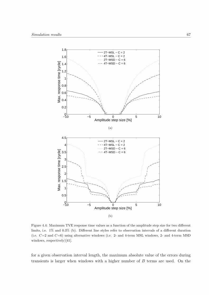
Simulation results 67
−10 −5 0 5 100
0.2
0.4
0.6
0.8
1
1.2
1.4
1.6
1.8
Amplitude step size [%]
Max
. res
pons
e tim
e [c
ycle
]
2T−MSL − C = 24T−MSL − C = 22T−MSD − C = 64T−MSD − C = 6
(a)
−10 −5 0 5 100
0.5
1
1.5
2
2.5
3
3.5
4
4.5
Amplitude step size [%]
Max
. res
pons
e tim
e [c
ycle
]
2T−MSL − C = 24T−MSL − C = 22T−MSD − C = 64T−MSD − C = 6
(b)
Figure 4.4: Maximum TVE response time values as a function of the amplitude step size for two different
limits, i.e. 1% and 0.3% (b). Different line styles refer to observation intervals of a different duration
(i.e. C=2 and C=6) using alternative windows (i.e. 2- and 4-term MSL windows, 2- and 4-term MSD
windows, respectively)[41].
for a given observation interval length, the maximum absolute value of the errors during
transients is larger when windows with a higher number of B terms are used. On the

68 A Dynamic DFT-based Synchrophasor Estimator
contrary, the response times are shorter since the window function in the time domain
decreases more quickly to zero when the number of terms grows [43]. This behavior is
confirmed also in Fig. 4.4, which displays the maximum TVE response time values as a
function of the amplitude step size for two different limits, i.e. 1% (a) (as recommended
in [18] for the whole PMU) and 0.3% (b) (assuming that the estimation accuracy due
to the algorithm only exceeds no more than 1/3 of the total PMU target accuracy). In
the figure, different line styles refer to four different estimators, i.e. 2- and 4-term MSL
windows over two-cycle observation intervals and 2- and 4-term MSD windows over six-
cycle observation intervals respectively. As expected, the response times are lower when
the observation intervals are shorter, but they grow when the limit decreases. In fact, the
TVE patterns need more time to settle below a lower limit. The discontinuous behavior
of the curves in Fig. 4.4(b) is due to the TVE ripples (like those shown in Fig. 4.4(a)),
which cross the 0.3% limit not just once (like in the 1% case), but multiple times before
lying steadily below 0.3%. The worst-case TVE response time curves resulting from phase
steps in the range [−10, 10] are quite similar to those shown in Fig. 4.4 and exhibit a
similar dependence on both observation interval length and number of window terms (the
corresponding curves are not reported for the sake of brevity). However, the maximum
response time values due to phase steps are slightly larger than those due to amplitude
steps. This behavior is confirmed in Tables 4.2 - 4.3, which reports a more compact
and exhaustive comparison between the maximum TVE response times associated with
different IpD2FT-based estimators, when either ±10% amplitude steps or ±10 phase
steps occur. All numbers are expressed in terms of nominal waveform cycles. Again, the
results in the Table refer to four iterations of the IpD2FT algorithm with the Taylor’s
series truncated to order K=2 and in three different pairs of configurations, i.e.
• using a 2- or a 4-term MSL windows over two-cycle observation intervals (C=2);
• using a 2- or a 4-term MSL windows over four-cycle observation intervals (C=4);
• using a 2- or a 4-term MSD windows over six-cycle observation intervals (C=6).
Two sets of limits are considered in each case, i.e. those reported in the Standard [18]
for the whole PMU and three smaller thresholds chosen arbitrarily under the assumption
that the maximum estimation errors due to the algorithm only is at most a fraction
of the total PMU accuracy limits reported in the Standard i.e. TV Elim = 0.3%. The
values shadowed in Tables 4.2-4.3 refer to those conditions that do not meet the P-Class
compliance boundaries, namely 1.7 nominal waveform cycles for TVE. Consider that
the M-class response time boundaries in the Standard depend on the reporting rate, but
in any case they are larger than the corresponding P-class values. Therefore, results
in Tables 4.2-4.3 that are compliant with P-class requirements are also compliant with

Simulation results 69
Table 4.2: Maximum TVE response time of the IpD2FT-based estimator with the Taylor’s series truncated
to order K=2, as a result of amplitude step changes. All values (expressed in nominal waveform cycles)
are computed in nominal frequency conditions from the instant when TVE exceeds the respective limits
(TVElim) to the time after which they permanently stay below such limits. The red values refer to the
conditions that violate the P Class boundaries reporte in the Standard [41].
Test type Amplitude step (±10%)
Window length C=2 C=4 C=6
Window type MSL MSL MSD
B=2 B=4 B=2 B=4 B=2 B=4
TVElim [%] 1 0.6 0.5 1.2 0.9 1.6 1.1
0.3 1.6 1.3 3.0 2.2 4 2.9
Table 4.3: Maximum TVE response time of the IpD2FT-based estimator with the Taylor’s series truncated
to order K=2, as a result of phase step changes. All values (expressed in nominal waveform cycles) are
computed in nominal frequency conditions from the instant when TVE exceeds the respective limits
(TVElim) to the time after which they permanently stay below such limits. The red values refer to the
conditions that violate the P Class boundaries reporte in the Standard [41].
Test type Phase step ( ±10)
Window length C=2 C=4 C=6
Window type MSL MSL MSD
B=2 B=4 B=2 B=4 B=2 B=4
TVElim [%] 1 0.9 0.8 1.3 1.0 1.8 1.3
0.3 1.8 1.4 3.4 2.6 4.5 3.3
M-class. In general, four-cycle observation intervals assure a good trade-off between
accuracy and responsiveness. However, by increasing the observation interval length,
responsiveness degrades. It is quite interesting to observe that when TVElim = 1% the
maximum TVE response times over C=4 cycles are comparable with those obtained with
a four-cycle TWLS estimator based on a Kaiser window with β=8 (i.e. about 1 cycle) as
shown in Chapter 3. On the contrary, when TVElim = 0.3% the TWLS responsiveness is
considerably better (i.e. slightly longer than 1 cycle against 2 to 3 cycles in the case of the
proposed algorithm). Probably this is due to the smaller size of the TVE ripples resulting
from the application of both the TWLS estimator and the adopted window [39]. The
transient behavior of the IpD2FT-based algorithm during ramps of system frequency has
been also analyzed in the worst-case conditions described in [18], i.e. by choosing different
random initial phases in [0, 2π] and by changing linearly the fundamental frequency from
f0− 5 Hz to f0+5 Hz at a rate of 1 Hz/s. Again, the algorithm relies on the second order
(K=2) and the same observation interval lengths and window types described previously,

70 A Dynamic DFT-based Synchrophasor Estimator
i.e. 2- and 4-term MSL windows over C=2 cycles, 2- and 4-term MSL windows over C=4
cycles and 2- and 4-term MSD windows over C=6 cycles. The corresponding maximum
values of TVE normalized by the respective worst-case thresholds reported in the Standard
(i.e. TVEramp = 1% for M-class compliance) are reported in Table 4.4.
Table 4.4: Maximum TVE values obtained using the IpD2FT-based estimator with the Taylor’s series
truncated to order K=2 for linear frequency ramp changes in [f0−5,f0 +5] Hz. All values are normalized
by the worst-case threshold reported in the Standard [18], i.e. TVEramp=1%.
Test type Frequency ramp
Window length C=2 C=4 C=6
Window type MSL MSL MSD
B=2 B=4 B=2 B=4 B=2 B=4
TVElim[%] 1 0 0.09 0.01 0 0.01 0
4.4 The problem of Phasor Angle Estimation
Various recent research works have emphasized the importance of measuring current or
voltage phasor angle with high accuracy at the distribution level. Indeed, the phase offsets
of the waveforms in different points of distribution networks are normally quite small, but,
at the same time, they may vary considerably (both in terms of amplitude and speed),
as a result of significant changes in generation or load profiles. In fact, active distribu-
tion networks are characterized by reduced line lengths, limited power flows and higher
distortion levels than those of transmission networks [45]. Such features suggest that
the PMU accuracy requirements at the distribution level are expected to be higher than
those specified in the Standard C37.118.1-2011, although no phase measurement uncer-
tainty limits are explicitly reported in [18] and [46]. In addition, at the distribution level
the PMUs could be used to monitor electromechanical transients, which generally lead to
non-negligible deviations from the nominal frequency. As a result, synchrophasors angles
could be poorly estimated if waveform frequency changes within the chosen observation
intervals are too relevant to be accurately measured. Moreover, both voltage magnitudes
and phases greatly depend on the levels of demand and distributed generation at a given
time [47]. Therefore, a PMU for distribution systems should not only track waveform
phasors, frequency and ROCOF in real-time under dynamic conditions [34],[39], but it
should be also able to measure phasor angles with uncertainty in the order a few mrad or
less [48], as it is confirmed by the specifications of some novel instruments currently under
development [49]. Generally, the phase errors result from three main contributions, i.e.
unwanted phase shifts introduced by instrument transformers (which are in the order of a

The problem of Phasor Angle Estimation 71
few crad) [50], offsets caused by the estimation algorithm itself and deviations due to the
limited time synchronization accuracy [51] or, sometimes, to the need to reconstruct the
phasor values at times different from tr [52]. The contribution of instrument transformers
is not related to the PMU, so it is out the scope of this section. The uncertainty contribu-
tions due to the synchrophasor estimation algorithm is probably the most interesting, as
it depends also on the features of the signals to be monitored. Since this issue is seldom
considered in the literature, in this section the angle measurement accuracy of three al-
gorithms, namely the classic DFT (3.3), the TWLS (3.6) and the IpD2FT (4.5)–(4.14), is
extensively analyzed. In all cases, the worst-case phasor angle measurement uncertainty
of the three considered estimators has been evaluated, simply computing Argpr.
4.4.1 Simulation and results
The accuracy of the considered phasor angle estimators has been evaluated through exten-
sive Monte Carlo simulations in various conditions based on the Standards C37.118.1-2011
and EN 50160-2010 [18],[53]. In fact, the latter document is specifically focused on power
quality requirements at the distribution level and it “specifies the main characteristics of
the voltage at a network user’s supply terminals in low, medium and high voltage AC elec-
tricity networks under normal operative conditions” [53]. Moreover, in order to test the
accuracy of the phasor angle estimators in transient conditions closer to those of distribu-
tion networks, some additional simulations under the influence of decaying DC offsets are
reported at the end of the tests. The choice of using two sets of testing conditions (and in
some case their combination) is due to the fact that the Standard C37.118.1-2011 (along
with its Amendment C37.118.1a-2014 [46]) deals with PMU performance regardless of how
or where these instruments are used. On the contrary, the Standard EN 50160-2010 is
specifically focused on the features of the voltage waveforms at the distribution level. All
simulations rely on the same general assumption used in Section 4.3. The absolute values
of the maximum phase errors associated with the DFT, IpD2FT and TWLS estimation
algorithms are shown in Tables 4.5, 4.6 and 4.7, respectively. All data are expressed in
mrad. The tests taken into consideration comprise the same conditions already used to
build Tab. 4.1, i.e. (case a – g), but includes a few additional ones, which are likely to
better represent the operating conditions of active distribution networks, i.e.
h) the fundamental frequency is assumed to be nominal, but the collected waveform is
affected by an amplitude step of magnitude equal to ±10% of the nominal value;
i) the fundamental frequency is assumed to be nominal, but the collected waveform
is affected by a phase step of ±10 (i.e. ±π/18), according with the worst-case
conditions reported in [18];

72 A Dynamic DFT-based Synchrophasor Estimator
j) the waveform exhibits a fundamental frequency deviation δ in the range [−0.1, 0.1]
and it is perturbed by all harmonics till the 25th. Each harmonic amplitude is
compliant with the worst-case specified in the Standard EN 50160-2010 [53];
k) finally, we consider the superposition of the harmonic disturbances described in case
j with the AM and PM modulations described case f.
The results reported in Tables 4.5, 4.6 and 4.7 show the following considerations. In
the case of static off-nominal frequency deviations only (case a) the IpD2FT method is
slightly better than the TWLS approach and both techniques outperform the DFT-based
estimator. However, the maximum phase errors associated with any algorithm can be
made negligible by increasing the observation interval length. Such results are basically
the same as those obtained by changing linearly δ at a rate of 1 Hz/s, as described in the
case of ramp testing in [18] and [46], since this rate of change of frequency causes very
small frequency changes when considering short observation intervals.
In the presence of noise, case b, the DFT-based estimator provides the best accuracy,
while the dynamic estimators exhibit similar performances. Also, the standard deviations
of the estimation is reduced by using longer observation intervals.
The classic DFT-based approach is generally also less sensitive to harmonics than the
IpD2FT estimator, which in turn performs better than the TWLS algorithm in cases c),
d) and j). The higher sensitivity of the dynamic approaches to harmonics is mainly due
to the use of phasor derivatives. Again, in all cases considered the maximum phase errors
can be reduced by increasing the observation interval length.
Under the effect of amplitude and/or phase modulation, in cases e) and f), both the
TWLS technique and the IpD2FT algorithm outperform the classic DFT-based estimator,
as expected, since they take advantage of the dynamic phasor model. However, unlike
the previous cases, the accuracy of all techniques degrades when C grows. This is quite
intuitive because phasor changes are smoothed by longer intervals.
The considerations above suggest that, in the presence of both steady-state harmonic
distortion and modulations (case k), for a given type of window, the best accuracy results
from the trade-off between opposite trends. This is not clearly visible from Tables 4.5 -
4.7, since, with the chosen values of C, the effect of harmonics prevails over modulations.
As a consequence, the maximum phase errors for a given number of window terms B,
apparently decrease monotonically. However, further simulations confirm that, the phase
error values exhibit a growing trend as soon as, by increasing C, the effect of modulations
prevails over harmonic distortion.
When a large out-of-band interferer is close to the fundamental tone (case g) the phase
errors associated with all estimators become quite large. However, the DFT estimator is
much less sensitive to the out-of-band interferers than the IpD2FT algorithm. In turn,

The problem of Phasor Angle Estimation 73
Tab
le4.
5:M
axim
um
abso
lute
valu
esof
the
ph
ase
esti
mati
on
erro
rs(e
xp
ress
edin
mra
d)
ob
tain
edw
ith
the
class
icD
FT
-base
dp
haso
res
tim
ati
on
algo
rith
min
diff
eren
tte
stin
gco
nd
itio
ns.
2-,3
-or
4-te
rmM
SD
win
dow
sov
erob
serv
ati
on
inte
rvals
wit
ha
du
rati
on
bet
wee
nab
ou
t2
an
d6
wav
efor
mcy
cles
.
Case
Test
conditions
Max
[mra
d]
2-term
MSD
3-term
MSD
4-term
MSD
C=
2C
=3
C=
4C
=3
C=
4C
=5
C=
4C
=5
C=
6
aF
req.
dev
.only
[−10%,1
0%
]1|e
rr.|
3.5
1.5
0.8
0.2
0.1
0.0
0.0
0.0
0.0
bF
req.
dev
.[−
10%,1
0%
]1+
|err
.bia
s|0.1
0.1
0.1
0.1
0.1
0.1
0.1
0.1
0.1
nois
e(S
NR
=40
dB
)er
r.st
d.
dev
.1.3
1.1
0.7
0.7
0.7
0.6
0.7
0.6
0.6
cF
req.
dev
.+2nd
harm
.(1
0%
)1|e
rr.|
15.6
4.3
1.5
6.4
0.5
0.1
3.0
0.1
0.0
dF
req.
dev
.+3rd
harm
.(1
0%
)1|e
rr.|
4.3
1.5
0.8
0.2
0.1
0.0
0.0
0.0
0.0
eF
req.
dev
.+A
M1
|err
.|8.5
12.8
19.9
7.2
12.2
18.5
8.8
13.5
19.0
fF
req.
dev
.+A
M1+
PM
1|e
rr.|
10.4
16.8
28.2
10.3
17.8
26.5
13.0
19.4
26.6
g10%
out-
of-
band
inte
rfer
ers1
|err
.|50.0
17.3
0.8
38.9
16.5
4.3
29.9
14.1
5.0
h10%
magnit
ude
step
1|e
rr.|
8.1
5.2
3.9
6.9
5.1
4.1
6.2
4.9
4.1
i10
phase
step
1|e
rr.|
102
96.4
94.0
99.4
96.2
94.4
98.1
95.9
94.4
jF
req.
dev
.+25
harm
.(1
0%
)2|e
rr.|
5.8
2.0
0.9
1.4
0.1
0.0
0.6
0.0
0.0
kF
req.
dev
.+A
M1+
PM
1+
25
harm
.2|e
rr.|
13.6
17.8
28.8
11.4
17.7
26.6
13.3
19.1
27.1
1C
ondit
ions
com
pliant
wit
hth
ere
quir
emen
tsof
the
Sta
ndard
IEE
EC
37.1
18.1
-2011
2C
ondit
ions
com
pliant
wit
hth
ere
quir
emen
tsof
the
Sta
ndard
EN
50160-2
010

74 A Dynamic DFT-based Synchrophasor Estimator
Tab
le4.6
:M
axim
um
ab
solu
tevalu
esof
the
ph
aseestim
atio
nerro
rs(ex
pressed
inm
rad
)ob
tained
with
the
classicIp
D2F
Tp
hasor
estimation
algorith
mfo
rK
=2
ind
ifferen
ttestin
gco
nd
itions.
2-,3-
or
4-term
MS
Dw
ind
ows
overob
servationin
tervalsw
itha
du
rationb
etween
ab
out
2an
d
6w
aveform
cycles
Case
Test
conditio
ns
Max
[mra
d]
2-te
rmM
SD
3-te
rmM
SD
4-te
rmM
SD
C=
2C
=3
C=
4C
=3
C=
4C
=5
C=
4C
=5
C=
6
aF
req.
dev
.only
[−10%,1
0%
] 1|err.|
0.0
0.0
0.0
0.0
0.0
0.0
0.0
0.0
0.0
bF
req.
dev
.[−
10%,1
0%
] 1+
|err.bia
s|0.1
0.1
0.1
0.1
0.1
0.1
0.1
0.1
0.1
noise
(SN
R=
40
dB
)err.
std.
dev
.1.1
0.9
0.8
1.0
0.9
0.8
0.9
0.9
0.8
cF
req.
dev
.+2nd
harm
.(1
0%
)1
|err.|71.9
21.9
2.8
46.9
12.6
0.6
28.7
7.6
0.4
dF
req.
dev
.+3rd
harm
.(1
0%
)1
|err.|2.8
0.4
0.2
0.1
0.0
0.0
0.0
0.0
0.0
eF
req.
dev
.+A
M1
|err.|2.1
0.8
1.0
0.3
0.5
1.1
0.3
0.7
1.4
fF
req.
dev
.+A
M1+
PM
1|err.|
2.1
0.8
1.2
0.3
0.6
1.4
0.4
0.8
1.7
g10%
out-o
f-band
interferers
1|err.|
98.3
73.9
43.3
85.4
64.3
39.2
75.6
55.2
34.4
h10%
magnitu
de
step1
|err.|14.9
9.5
7.2
12.6
9.1
7.1
10.6
8.3
6.9
i10
phase
step1
|err.|117
105
100
109
103
100
106
102
99.2
jF
req.
dev
.+25
harm
.(1
0%
)2
|err.|15.7
4.4
0.6
9.4
2.5
0.1
5.7
1.5
0.1
kF
req.
dev
.+A
M1+
PM
1+25
harm
. 2|err.|
16.4
5.2
1.6
10.4
3.1
1.4
6.3
2.3
1.7
1C
onditio
ns
com
plia
nt
with
the
requirem
ents
of
the
Sta
ndard
IEE
EC
37.1
18.1
-2011
2C
onditio
ns
com
plia
nt
with
the
requirem
ents
of
the
Sta
ndard
EN
50160-2
010

The problem of Phasor Angle Estimation 75
Tab
le4.
7:M
axim
um
abso
lute
valu
esof
the
ph
ase
esti
mati
on
erro
rs(e
xp
ress
edin
mra
d)
ob
tain
edw
ith
the
class
icT
WL
Sp
haso
res
tim
ati
on
algo
rith
mfo
rK
=2
ind
iffer
ent
test
ing
con
dit
ion
s.2-
,3-
or
4-t
erm
MS
Dw
ind
ows
over
ob
serv
ati
on
inte
rvals
wit
ha
du
rati
on
bet
wee
nab
ou
t2
an
d
6w
avef
orm
cycl
es
Case
Test
conditions
Max
[mra
d]
2-term
MSD
3-term
MSD
4-term
MSD
C=
2C
=3
C=
4C
=3
C=
4C
=5
C=
4C
=5
C=
6
aF
req.
dev
.only
[−10%,1
0%
]1|e
rr.|
0.6
0.0
0.0
0.2
0.0
0.0
0.0
0.0
0.0
bF
req.
dev
.[−
10%,1
0%
]1+
|err
.bia
s|0.1
0.1
0.1
0.1
0.1
0.1
0.1
0.1
0.1
nois
e(S
NR
=40
dB
)er
r.st
d.
dev
.1.2
1.0
0.8
1.1
0.9
0.8
1.0
0.9
0.8
cF
req.
dev
.+2nd
harm
.(1
0%
)1|e
rr.|
84.9
38.2
6.3
67.3
35.6
12.4
55.4
30.6
12.6
dF
req.
dev
.+3rd
harm
.(1
0%
)1|e
rr.|
3.1
0.3
0.0
1.0
0.0
0.0
0.2
0.0
0.0
eF
req.
dev
.+A
M1
|err
.|0.8
0.4
1.0
0.3
0.4
0.9
0.2
0.5
0.9
fF
req.
dev
.+A
M1+
PM
1|e
rr.|
1.1
0.6
1.8
0.5
0.7
1.7
0.4
0.9
1.8
g10%
out-
of-
band
inte
rfer
ers1
|err
.|107
83.6
59.1
96.8
80.4
63.0
89.9
77.1
61.9
h10%
magnit
ude
step
1|e
rr.|
20.7
11.6
8.4
16.6
11.5
9.0
14.3
11.0
9.0
i10
phase
step
1|e
rr.|
122
107
102
116
107
103
112
107
103
jF
req.
dev
.+25
harm
.(1
0%
)2|e
rr.|
17.4
7.7
1.3
13.6
7.1
2.5
11.2
6.1
2.5
kF
req.
dev
.+A
M1+
PM
1+
25
harm
.2|e
rr.|
18.4
8.7
3.0
14.9
8.2
3.3
12.3
7.2
3.6
1C
ondit
ions
com
pliant
wit
hth
ere
quir
emen
tsof
the
Sta
ndard
IEE
EC
37.1
18.1
-2011
2C
ondit
ions
com
pliant
wit
hth
ere
quir
emen
tsof
the
Sta
ndard
EN
50160-2
010

76 A Dynamic DFT-based Synchrophasor Estimator
this is less sensitive than the TWLS estimator. Also, accuracy improves as the observation
interval length increases since the frequency distance between the fundamental component
and the interfering tone increases.
The maximum phase errors associated with the three estimators in transient condi-
tions, i.e. under the effect of amplitude steps (case h) or phase steps (case i), respectively
are also reported in the Tables. The DFT estimator is less sensitive to transients than
the IpD2FT algorithm. This, however, performs clearly better than the TWLS. As ex-
pected, the maximum error due to a phase step is much larger than the maximum error
related to a magnitude step, as the former impacts directly on the phase of the waveform.
Observe that in all the considered cases the errors tend to decrease, even if slowly, as
the observation interval length grows. When the IpD2FT algorithm is considered, the
number of terms of the Taylor’s series deserves a special attention. Indeed, if K increases
(e.g. K=3), the observation interval length has to increase as well to avoid significant
spectral interferences due to other spectral components such as harmonics or the image
tone. As a result, the IpD2FT algorithm responsiveness degrades, but accuracy tends to
slightly improve by using K=3 rather than K=2. However, by increasing K the algorithm
becomes more sensitive to wideband noise (i.e. in case b). Ultimately, K=2 provides a
good trade-off between overall accuracy and responsiveness.
In Fig. 4.5 the maximum absolute values of the phase estimation errors associated with
the DFT-based technique (a), the IpD2FT algorithm (b), and the TWLS estimator (c),
respectively, are compared in the testing conditions related to case j. The error curves
are plotted as a function of δ for C = B+ 2 cycles when a B− term MSD window is used
(with B = 2, 3 or 4). The plots confirm that the DFT-based solution is slightly more
robust to harmonics than the others. However, the TWLS estimator can be significantly
affected by harmonics when δ is negative.
Fig. 4.6 shows the maximum absolute values of the phase estimation errors associated
with the DFT-based technique (a), the IpD2FT algorithm (b), and the TWLS estimator
(c), under the testing conditions related to the (case f ). The adopted windows and the
observation interval lengths are the same as those used in Fig. 4.5. However, in this
case the IpD2FT algorithm and the TWLS estimator clearly outperform the classic DFT–
based approach.
Fig 4.7(a)-(b) provides an example of the transient behavior of all the analyzed es-
timators under the testing conditions related to the cases h) and i), respectively. In
Fig. 4.7(a)-(b) the maximum phase error envelopes associated with the three estimators
are plotted as a function of time expressed in nominal waveform cycles, when the ob-
servation interval is about C = 4 cycles long and a 2-term MSD window is used. The
curves confirm that when an amplitude step occurs the maximum error introduced by the

The problem of Phasor Angle Estimation 77
−10 −5 0 5 100
0.2
0.4
0.6
0.8
1
δ [%]
Max
. |P
hase
Err
or| [
mra
d]
2−term MSD, C=4
3−term MSD, C=5
4−term MSD, C=6
(a)
−10 −5 0 5 100
0.2
0.4
0.6
0.8
1
δ [%]
Max
. |P
hase
Err
or| [
mra
d]
3−term MSD, C=5
2−term MSD, C=4
4−term MSD, C=6
(b)
−10 −5 0 5 100
0.5
1
1.5
2
2.5
3
δ [%]
Max
. |P
hase
Err
or| [
mra
d]
2−term MSD, C=4
3−term MSD, C=5
4−term MSD, C=6
(c)
Figure 4.5: Maximum absolute values of the phase estimation errors associated with the classic DFT-
based technique (a), the IpD2FT algorithm (b), and the TWLS estimator (c), as a function of the static
off-nominal frequency deviation δ and under the effect of a worst-case total harmonic distortion compliant
with the Standard EN 50160:2010.

78 A Dynamic DFT-based Synchrophasor Estimator
−10 −5 0 5 105
10
15
20
25
30
δ [%]
Max
. |P
hase
Err
or| [
mra
d]
3−term MSD, C=5
2−term MSD, C=4
4−term MSD, C=6
(a)
−10 −5 0 5 100
0.5
1
1.5
2
δ [%]
Max
. |P
hase
Err
or| [
mra
d]
3−term MSD, C=5
2−term MSD, C=4
4−term MSD, C=6
(b)
−10 −5 0 5 100
0.5
1
1.5
2
δ [%]
Max
. |P
hase
Err
or| [
mra
d]
4−term MSD, C=6
3−term MSD, C=5
2−term MSD, C=4
(c)
Figure 4.6: Maximum absolute values of the phase estimation errors associated with the DFT-based
technique (a), the IpD2FT algorithm (b), and the TWLS estimator (c), under the joint effect of: static
off-nominal frequency deviations δ 6= 0, amplitude modulation (AM) and phase modulation (PM). The
modulating signals are two sine-waves of amplitude equal to 10% of the fundamental and 0.1 rad for AM
and PM, respectively, and frequencies equal to 0.1 · f0.

The problem of Phasor Angle Estimation 79
−2 −1 0 1 2 3 4 50
1
2
3
4
5
6
7
8
9
Number of cycles
Max
. |P
hase
Err
or| [
mra
d]
Amplitude step response
IpD2FT
TWLS
DFT
(a)
−2 −1 0 1 2 3 4 5−100
−50
0
50
100
Number of cycles
Max
. |P
hase
Err
or| [
mra
d]
Phase step response
IpD2FT
DFT
TWLS
(b)
Figure 4.7: Phase errors envelopes as a function of time (expressed in nominal waveform cycles) when
either a 10% magnitude step (a) or a 10 phase step occurs (b). Different line color refer to the DFT-
based technique, the IpD2FT algorithm and the TWLS estimator, when a 2-term MSD window is used
over a four-cycle observation interval. The small diamonds highlight when the step occurs.

80 A Dynamic DFT-based Synchrophasor Estimator
DFT-based estimator is generally smaller than the maximum error associated with the
IpD2FT algorithm or by the TWLS technique. Conversely, in the presence of phase steps,
errors are much larger and quite similar. Quite interestingly, the duration of transients
is almost the same for all estimators in both case h) and case i). Additional simulation
results, not reported for the sake of brevity, show that the error peaks during transients
are almost proportional to the step size, both in magnitude or in phase.
Since the effect of transients is particularly interesting in the case of distribution net-
works, some additional results under the influence of decaying DC offsets are reported
in Fig. 4.8. The three curves displayed on Fig.4.8 with different line styles represent the
maximum phase errors associated with the three considered estimators, when the observa-
tion interval is C=5 cycles and a 3-term MSD window is used. In all cases, exponentially
decreasing DC offsets with initial amplitude equal to 70% of the fundamental and time
constant τ in the range between 0.1 and 10 s are added to a sinusoidal voltage waveform
of frequency f0 [54]. Each point of the curves is the maximum phase error resulting from
200 initial phase values chosen at random in [0, 2π). The decaying DC offset always start
at the beginning of the observation intervals. The reported results show that the DFT
approach is the least sensitive to the influence of such disturbances. Accuracy is about one
order of magnitude worse for the IpD2FT algorithm and at least two orders of magnitude
0 2 4 6 8 1010
−3
10−2
10−1
100
101
102
τ [s]
Max
. |P
hase
Err
or| [
mra
d]
TWLS
IpD2FT
DFT
Figure 4.8: Maximum phase errors as a function of the time constant of an additive decaying DC offset
of initial amplitude equal to 70% of the nominal waveform amplitude. Different line color refer to the
DFT-based technique, the IpD2FT algorithm and the TWLS estimator, respectively, when a 3-term MSD
window is used over a five-cycle-long observation interval.

Jitter and time alignment uncertainty 81
worse than the TWLS estimator. By changing the observation interval length or the type
of window, similar patterns are obtained. Observe that the phase errors associated with
the DFT and IpD2FT estimators exhibit a monotonically decreasing trend. This is due to
the fact that when τ grows, the spectral content of the decaying DC offsets is increasingly
concentrated around zero, i.e. faraway from the spectral samples used by the algorithms.
On the contrary, the sensitivity of the TWLS estimator to decaying DC offsets is not only
larger, but it is also almost independent of the values of τ . This is due to the fact that
the TWLS estimator relies on the weighted least square fitting in the time domain of a
dynamic (i.e. oscillating) phasor model, which does not include any decaying DC offset.
Therefore, such terms cannot be tracked with good accuracy regardless of the value of τ .
4.5 Jitter and time alignment uncertainty
The analysis performed in the previous sections was focused on the effect of phasor es-
timation algorithms only. However, as stated in the Section 4.4, additional uncertainty
contributions arise from: sampling jitter, limited synchronization accuracy, and the need
to estimate the phase of a waveform at times different from the center of the considered
observation interval. The sampling jitter depends on the fact that even if the sampling
clock is disciplined by a GPS receiver or by some other synchronization technique (e.g.
the IEEE 1588 Precision Time Protocol [55]), the input waveform within the rth obser-
vation interval is actually sampled at times which slightly differ from tr + nTs. If we
denote with δT the random time fluctuations of the sampling period Ts, the equivalent
effect of this term on phasor estimation algorithms is to inject an additional phase modu-
lation term in the signal model. This means that εpr [n] in (4.1) should be rather replaced
by ε′pr [n] = εpr [n] + 2π∑n
i=0 δTs [i]. In addition, because of the limited synchronization
accuracy, even if the delays due to the acquisition stage are properly estimated and com-
pensated, the phase in the center of the considered observation interval is affected by
some uncertainty. In particular, if tj models the synchronization uncertainty, then the
corresponding phase uncertainty at reference time tr can be approximated by a first-order
Taylor series expansion as follows:
∆ϕjr ≈(
2πf0(1 + δ) +dεpdt|t=tr
)tj. (4.16)
In practice, the values of tj usually range from some hundreds of ns to a few µs. For
instance, if the worst-case synchronization uncertainty is 1 µs, the absolute value of the
maximum phase error ∆ϕjmax is about 0.4 mrad, i.e. smaller than (or at most comparable
to) the algorithm-related phasor estimation errors in most of the conditions considered.

82 A Dynamic DFT-based Synchrophasor Estimator
A further uncertainty contribution affecting phasor angle measurements arises from
the need to reconstruct the phasor data at times different from the reported ones. In fact,
the PMU reporting rate depends on various factors, such as the performance class of the
instrument (i.e. P-class or M-class [18]), the specific features of the PMU employed and
the chosen instrument settings. When multiple streams of data are collected by (PDC)
at different rates, all measurements results need to be aligned in time. In such cases, the
phasor angle ϕ′r at a generic time t′r = tr + ∆t results approximately from [52]
ϕ′r∼= ϕr + 2π
[(fr − f0)∆t+
∆t2
2ROCOFr
], (4.17)
where ϕr, fr and ROCOFr are the phase, the frequency and the ROCOF values at time
tr. In practice, both fr and ROCOFr are affected by some uncertainty that propagates
to the phase estimate. If we denote with FEr and RFEr as the frequency and ROCOF
measurement errors in the rth observation interval, it results immediately from (4.17)
that the phase error due to time alignment is:
∆ϕar = 2π
(FEr ·∆t+
∆2t
2·RFEr
). (4.18)
In [52] it is noticed that the maximum FE and RFE values in the steady-state conditions
reported in the Standard IEEE C37.118.1-2011 are too strict for P-class instruments and
too loose for M-class PMUs. In fact, new and more sensible limits have been recently pub-
lished in an Amendment to the same Standard [46]. In steady-state conditions (namely
in the presence of off-nominal frequency deviations, harmonics and/or out-of-band inter-
ferers) the new FE and RFE upper bounds for P-class PMUs are 0.005 Hz and 0.4 Hz/s,
respectively. In the case of M-class instruments instead, the scenario is more complex as
the maximum FE values are 0.0025 Hz, 0.005 Hz, or 0.01 Hz depending on the consid-
ered testing condition, while the RFE limit is specified only in the off-nominal case (0.1
Hz/s). In dynamic conditions (particularly, when significant amplitude or phase modu-
lations occur), depending on the PMU reporting rate, the FE and RFE limits lie in the
following intervals: [0.03, 0.06] Hz and [0.6, 2.3] Hz/s, respectively, for a P-class PMU and
[0.12, 0.30] Hz and [2.3, 14] Hz/s for an M-class PMU. By replacing the maximum values
reported above in to (4.18) and noticing that the time misalignment ∆t could be up to 70
ms for a P-class PMU, or up to 300 ms for an M-class PMU [52], it follows immediately
that the worst-case phase errors ϕamax are:
• up to about 8 mrad in steady-state conditions and up to about 62 mrad in dynamic
conditions when considering P-class PMUs;
• up to about 47 mrad in steady-state conditions and between about 350 mrad (fast
reporting rates) to about 876 mrad (slow reporting rates) under the effect of modu-
lations for P-class PMUs.

Conclusion 83
Thus, the time alignment uncertainty may quickly become the main contributor to the
overall phase error.
4.6 Conclusion
In this chapter, a novel synchrophasor estimation algorithm based on a dynamic model is
presented and analyzed in various steady-state and transient conditions. Several simula-
tion results suggest that using a proper MSL window most of the M-class requirements of
the Standard IEEE C37.118.1-2011 can be met using four-cycle observation intervals. The
main uncertainty contribution affecting synchrophasor estimation accuracy are harmon-
ics, wideband noise and out-of-band interferers. By increasing the observation interval
duration, their impact decrease. However, the responsiveness in presence of amplitude or
phase step changes and the estimation accuracy under the effect of amplitude or phase
fluctuations degrade.
The second part of this chapter is focused on the phasor angle estimation accuracy
of three different algorithms (i.e. the classic DFT-based algorithm, the Interpolated Dy-
namic DFT algorithm (IpD2FT) and Taylor Weighted Least Square (TWLS)), with a
special attention to the disturbances at the distribution level. Using a common set of
window functions and observation intervals, it turns out that the classic DFT-based es-
timator is less sensitive to harmonics, out-of-band interferers, amplitude or phase steps.
The IpD2FT and TWLS estimators instead are particularly accurate in the presence of
waveform amplitude and/or phase fluctuations. While the TWLS technique is globally
slightly better in dynamic conditions, the IpD2FT algorithm exhibits a lower sensitivity
to steady-state disturbances, step-like changes and decaying DC offsets. Apparently, no
estimator is able to provide best results in all situations. In addition, the accuracy of all
the considered methods can be strongly affected by quick frequency or phase variations,
as it may happen during transients. Finally, it is worth emphasizing that even though
sampling and synchronization jitter have usually a minor impact on the overall phase
error, possible time misalignments between the results returned by different PMUs (e.g.
due to frequency and ROCOF limited measurement accuracy) could lead to intolerably
large phase errors.

84 A Dynamic DFT-based Synchrophasor Estimator

Chapter 5
State Estimation and Measurement
Uncertainty Sensitivity
As known, electrical quantities, such as voltages, currents as well as active and reactive
powers, have to be continuously monitored by system operators in order to use them for
grid state estimation (SE). Currently, the SE requirements in terms of accuracy and re-
sponsiveness are changing as a result of smart grid evolution. In this context, the accurate
measurement data coming from PMUs can substantially enhance SE and the correspond-
ing applications. The purpose of this chapter is to review the definition, the properties and
the sensitivity to measurement uncertainty of one of the most commonly used algorithms
for SE, i.e. the Weighted Least Squares (WLS) technique. Even though the SE problem
has been traditionally focused on transmission networks, currently and, even more in the
future, distribution system state estimation (DSSE) is envisioned to become of primary
importance for correct grid operation. In fact, the traditional sharp distinction between
transmission and distribution networks (whose features were clearly different in the past)
is expected to blur in grids where widespread micro-generation and dynamic load changes
will bring about significant and time-varying bidirectional power flows [56]. Since the
definition and the properties of WLS-based SE are basically the same in both contexts, a
proper and general mathematical analysis of the sensitivity of this technique to different
kinds of measurements is important to minimize their number, regardless of technology-
or budget-related constraints. This problem is not totally new as it was already investi-
gated some years ago [57]. For instance, [58] includes various analytical expressions that
can be used to evaluate how measurement schemes, transmission line modeling, and other
Part of this chapter was published in
D. Macii, G. Barchi, D. Petri, “Uncertainty sensitivity analysis of WLS-based grid state estimators,” IEEE
International Workshop on Applied Measurements for Power Systems Proceedings (AMPS), 2014,vol., no., pp.1,6,
24-26 Sept.2014.

86 State Estimation and Measurement Uncertainty Sensitivity
network parameters affect the goodness of a state estimate. However, this chapter will
be specifically focused on the sensitivity analysis to measurement uncertainty, assuming
that just a minimum amount of measurements is used to assure full state observability.
5.1 Introduction on SE
In the field of power systems, state estimation (SE) refers to the set of algorithms and
techniques that combine measurement results, network topology, and network parameter
values to determine the state of a grid at a given time [59]. Many management tasks like
voltage regulation, stability monitoring, contingency analysis and dispatching, depend on
knowledge of the state of the network. In the past, SE was mainly used at the transmission
level, where the measurement data are collected through the network and provided by the
SCADA system at a certain time. A typical SCADA system relies on quasi-steady state
operative condition and it is unable to monitor fast transient phenomena. In the presence
of dynamic events, such as load variations or topology changes, the measurements provided
by SCADA can be affected by time skew due to the lack of synchronization, which can
lead inaccurate estimates of the system state [7].
Various SE techniques exist and they can be roughly classified as static or dynamic [7].
The main difference between them is that in the dynamic case, the evolution of state
variables over time is described by a dynamic system model based on a set of differential
or finite difference equations. In particular, the definition of an internal model relaxes
the need for measuring all the outputs of the system. In fact, a dynamic estimator, such
as a Kalman Filter, relies partially on the internal system model to achieve observability
and to track possible changes over time [60]. If no internal model are available, then just
a static estimator can be used. In this case, the state of the networks can be observed
only through at least so many independent measurements as the number of state variables.
The main drawback of dynamic estimators is that they are more difficult to apply because
they require good knowledge of the underlying model parameters. Moreover, the model
has to be robust enough to be usable in a variety of conditions.
In this chapter and in the following only static state estimators will be considered.
The most common used algorithm for SE is based on the Weighted Least Square (WLS)
method. Various formulation of the WLS-based SE approach exist. In the most classic
case the state variables are the magnitude and the angles of the nodal voltages; with the
network being described by a single-phase model. The three-phase formulation of the
same estimator is described in [61]. A dual SE approach where the state variables are
the branch currents expressed in Cartesian coordinates is instead formalized in [62]. Two
alternative formulations based on the same idea are reported in [63] and [64], respectively.

Measurement model and observability condition 87
5.2 Measurement model and observability condition
Let us consider a network composed by N buses and B lines. Generally, the state of the
network is modeled by x = [θT ,V T ]T where θT = [θ2, θ3, ..., θN ]T is the vector of the
voltage phasor angles at buses 2, ..., N (the phase of bus number 1 is usually taken as
a reference, i.e. θ1 = 0) and V T = [V1, V2, ..., VN ]T is the vector of the N bus voltage
magnitudes. In general, the state of the network can be observed through the well-known
measurement model [59], i.e.
z = h(x) + εz =
P flow(x)
P inj(x)
Qflow(x)
Qinj(x)
V (x)
θ(x)
I(x)
β(x)
+ εz (5.1)
where:
• h(x) is a nonlinear vector function of the state variables;
• P flow = [Pflow1,Pflow2
,. . .,PflowB ]T and Qflow = [Qflow1, Qflow2
, . . . , QflowB ]T are the
vectors of real and reactive power, respectively, flowing through network lines;
• P inj = [Pinj1 ,Pinj2 ,. . ., PinjN ]T and Qinj = [Qinj1 ,Qinj2 ,. . .,QinjN ]T are the vectors of
real and reactive power injected at bus n = 1, . . . , N ;
• V = [V1,V2,. . .,VN ]T and θ = [θ2,θ3,. . .,θN ]T are identity functions of the state, i.e.
V (x) = V and θ(x) = θ;
• I=[I1,I2,. . ., IB]T and β=[β1,β2,. . . ,βB]T are the magnitudes and the phases of the
line currents;
Note that εz is a column vector including all measurement uncertainty contributions. In
the following, we will refer to σ2i as the variance associated with the ith measurement. It
is worth emphasizing that x is a function of time, although the time variable is generally
omitted to keep notation simpler.
The explicit expression of P flow(x), P inj(x),Qflow(x),Qinj(x), I(x), β(x) are widely
available in the literature, e.g. in [59]. If we assume that each network branch is described

88 State Estimation and Measurement Uncertainty Sensitivity
k mgkm bkm
gsk+jbsk gsm+jbsm
Figure 5.1: Two-port π-model of a network branch [59].
by the two-port π model shown in Fig. 5.1 and that Ykm = Gkm + Bkm is the element
(k,m) of the network bus admittance matrix, the following expressions hold [59]:
• the real and reactive power injection at bus k are
Pinjk = Vk∑m∈Nk
Vm(Gkm cos θkm +Bkm sin θkm) (5.2)
Qinjk = Vk∑m∈Nk
Vm(Gkm sin θkm −Bkm cos θkm); (5.3)
• the real and reactive power flow from bus k to bus m are given by
Pflowkm =V 2km(gsk + gkm)−VkVm(gkm cos θkm + bkm sin θkm) (5.4)
Qflowkm =−V 2km(bsk + bkm)−VkVm(gkm sin θkm − bkm cos θkm); (5.5)
• the real and imaginary part of the line current flow magnitude from bus k to bus m
are defined as
IREkm = Vk(gsk + gkm) cos θk− Vk(bsk+bkm) sin θk
− V (m)gkm cos θm+Vmbkm sin θm; (5.6)
IIMkm= Vk(bsk + bkm) cos θk + Vk(gsk + gkm) sin θk
− Vmbkm cos θm − Vmgkm sin θm; (5.7)
Thus the magnitude and the angle of the corresponding branch current is simply
given by:
Ikm =√I2REkm
+ I2IMkm
(5.8)
βkm = arctan
(IIMkm
IREkm
); (5.9)
In expression (5.2)-(5.9)
− Vk, θk are the voltage magnitude and phase angle at bus k, respectively;

The WLS state estimator 89
− θkm = θk − θm;
− gkm+jbkm is the admittance of the series branch connecting buses k and m;
− gsk + jbsk is the admittance of the shunt branch connected at bus k;
− Nk is the set of bus numbers that are directly connected to bus k.
Note that (5.1) may consists of up to M = 4N + 4B − 1 equations, but in practice just
a subset M ′ ≤M of them is typically used to estimate the 2N − 1 state variables. If the
network internal dynamic is generally supposed to be negligible (i.e. the linearized system
state matrix is a 2N−1×2N−1 identity matrix), then it can be easily proved from basic
systems theory that the state of the network is observable if and only if the observability
matrix associated with the linearized system around its state x = x(t) at a given time t
has a full column rank. This is indeed possible if and only if rankH(x) = 2N −1 where
H(x) =
∂P flow∂θ
∂P flow∂V
∂P inj∂θ
∂P inj∂V
∂Qflow∂θ
∂Qflow∂V
∂Qinj∂θ
∂Qinj∂V
∂V∂θ
∂V∂V
∂θ∂θ
∂θ∂V
∂I∂θ
∂I∂V
∂β∂θ
∂β∂V
(5.10)
is the Jacobian of h(x). Therefore, at least M ′=2N−1 measurement equations of (5.1)
with linearly independent coefficients in H(x) are needed to estimate x.
5.3 The WLS state estimator
The well-known WLS state estimator relies on the minimization of the cost function
J(x) = [z − h(x)]TR−1[z − h(x)], (5.11)
where R is the covariance matrix associated with the selected measurements. Usually, such
contributions are assumed to be uncorrelated (i.e. Eεziεzj = 0, ∀i 6= j = 1, . . . ,M ′,
where E· denotes the expectation operator). Therefore, R = diag(σ21, . . . , σ
2M ′). By
computing the gradient of J(x) and its Taylor series truncated to the first order around
xk for k ≥ 0, the state at iteration k+1 can be obtained using the Gauss-Newton method,
i.e. [59]
xk+1 =xk+[HT (xk)R−1H(xk)]
−1HT (xk)R−1(z−h(xk)). (5.12)

90 State Estimation and Measurement Uncertainty Sensitivity
Observe that (5.12) converges to a solution if and only if [HT (xk)R−1H(xk)]
−1 is nonsin-
gular, or, equivalently, if and only if rankH(xk) = 2N − 1 ∀k, in accordance with the
observability condition expressed in Section 5.2. Since, normally, at time t the iterative
Gauss-Newton method is supposed to converge to the actual state x, the WLS returns
meaningful results if and only if H(x) exhibits full column rank in a reasonably large
neighborhood of x. The flow chart of WLS algorithm is shown in Fig.5.2. However, it
is well known that WLS method suffers from possible of convergence problems due to
numerical instabilities, which may occur when R−1 is ill-conditioned or when virtual mea-
surements (e.g. zero-power injection) exist. In such cases, the standard WLS methods
can be modified by using the QR Chorlesky decomposition or the Lagrange multiplier
techniques.
Set index k=1
Calculate G(xk)
Calculate x
k=H(x
k)TR-1(z-h(x
k))
Start
Decompose G(xk)
and solve for Δxk
Initialize state vector xk
max |Δxk|≤ ?
End
YES
NOδmax
Figure 5.2: Flow chart of weighted least square method.

Uncertainty Sensitivity Analysis 91
5.4 Uncertainty Sensitivity Analysis
If εz is the vector of uncertainty contributions related to the available M ′ ≥ 2N − 1
measurements, it follows immediately from (5.12) that the vector εx of the estimation
errors associated to a generic state x results from
εx=F (x)εz (5.13)
where F (x) = [HT (x)R−1H(x)]−1HT (x)R−1 can be referred to as sensitivity matrix, as it
provides information about the effect of different measurements on the estimates of each
state variable. The covariance matrix of the state estimates is simply given by:
Φx=Eεx ·εTx =F (x)Eεz ·εTz F T(x)=F (x)RF T(x). (5.14)
Observe that if just a minimum set of measurements M ′ = 2N − 1 is used and if
rankH(x) = 2N − 1, then F (x) = H−1(x), which is independent of R. Since R is
a diagonal matrix comprising the absolute variances of the individual measured quanti-
ties, this can be rewritten as
R = ZRr, (5.15)
where:
• Z = diag(z21 , z
22 , . . . , z
2M ′) is a diagonal matrix including the squared values of the
electrical quantities that should be ideally observed if measurement uncertainty were
negligible (i.e. when εz ≈ 0);
• Rr = diag(σ2r1, σ2
r2, . . . , σ2
rM′) is the diagonal matrix built using the respective relative
measurement uncertainties (except in the case of phase measurement, where the
absolute uncertainty values are considered).
Thus, if M ′ = 2N − 1, expression (5.14) can be also rewritten as
Φx=H−1(x)ZWiH−1T (x)σ2
ri= UFiσ
2ri
(5.16)
where the weights of matrix Wi = diag(σ2r1
σ2ri
, . . . , 1, . . . ,σ2rM′σ2ri
) are the relative measurement
uncertainties with respect to the ith one chosen as a reference. In essence, (5.16) highlights
how the estimation uncertainty of each state variable depends on the uncertainty of the
ith measurement.
If no a-priori information about measurement uncertainty is available, a reasonable
approach to perform a global sensitivity analysis is to assume that σr1=. . .=σr2N−1=σr. In
this case, Wi is a (2N−1)× (2N−1) identity matrix and UFi = UF contains the increment
rates of the elements of the covariance matrix Φx with respect to σ2r . Even if assuming

92 State Estimation and Measurement Uncertainty Sensitivity
that all measurements are affected by the same uncertainty is not realistic in practice,
this approach provides a fair indication of the sensitivity of state estimation to different
kinds of measurements. As a result, some measurements could be included (or excluded)
a priori in (from) a possible experimental setup.
Unfortunately, UF consists of (2N −1)×(2N −1) values. Thus, even if it can be useful
to analyze the uncertainty sensitivity of individual state variables, it does not provide a
global overview of the sensitivity of the whole WLS state estimator to a generic set of
2N − 1 measurements. To this purpose, a scalar function combining all state estimation
errors should be defined.
The individual estimator errors can be potentially expressed in terms of vectorial
error, to take into account the joint effect of magnitude and phase estimation errors.
With reference to bus i = 1, . . . , N , the vector error associated to the ith bus voltage
phasor is defined as
εVEi= |(Vi + εVi)e
j(θi+εθi ) − Viejθi |
=√ε2Vi
+ 2 (Vi + εViVi) (1− cos εθi), (5.17)
where εθi and εVi are the phase and magnitude estimation errors. If the mean values of
the estimation errors εθ = [εθ1 , . . . , εθN ]T and εV = [εV1 , . . . , εVN ]T are negligible, from
a first-order Taylor series approximation of the square of (5.17) it can be easily shown
that
Eε2VEi ≈ Eε2
Vi+ ViEε2
θi i = 1, . . . , N. (5.18)
If the sensitivity matrix F (x) is split into two N ×M ′ matrices [F Tθ (x), F T
V (x)]T related
to vectors θ and V , respectively, (with an all-zeros row added on top of Fθ(x) to take
into account the state variable θ1 = 0) and if σr1=. . .=σr2N−1=σr, it follows from (5.14)
that
Eεθ ·εTθ = Fθ(x)ZF Tθ (x)σ2
r =Gθθ(x)σ2r
EεV ·εTV = FV (x)ZF TV (x)σ2
r =GV V (x)σ2r. (5.19)
Thus, we can define the following two global scalar performance parameters based on (5.18),
i.e. the root average mean square error
RAMSE =
√√√√ 1
N
N∑i=1
Eε2VEi = SAσr, (5.20)
and the root maximum mean square error
RMMS =√
maxi=1,...,N
Eε2VEi = SMσr. (5.21)

Uncertainty Sensitivity Optimization 93
If GV Vii(x) and Gθθii(x) are the ith elements of the main diagonal of GV V (x) and Gθθ(x),
respectively, it follows from (5.19) that
SA =
√√√√ 1
N
N∑i=1
(GV Vii(x) + V 2i Gθθii(x)) (5.22)
and
SM =√
maxi=1,...,N
(GV Vii(x) + V 2i Gθθii(x)). (5.23)
Expressions (5.22) and (5.23) provide the average and maximum measurement uncertainty
sensitivity of the WLS state estimator to a given set of 2N − 1 measurements. In the
following, we will refer to a measurement configuration or simply a configuration as any
set of M ′ = 2N − 1 measurements extracted from (5.1).
5.5 Uncertainty Sensitivity Optimization
In theory, the configuration characterized by i) a minimum amount of measurement points,
ii) full state observability and iii) minimum worst-case sensitivity to measurement uncer-
tainty, can be found by solving a constrained, nonlinear and combinatorial optimiza-
tion problem. Let ξ = [ξ1, ξ2, . . . , ξM ]T be a binary vector, whose ith element is set equal
to 1 if the ith measurement is used for state estimation or 0 otherwise. As it is explained
in Section 5.4, if M ′ = 2N − 1 measurements are considered, then F (x) = H−1(x). This
condition can be equivalently expressed by defining the expanded matrix
Fe(ξ,x) = [HTe (x)ΞHe(x)]−1HT
e (x)Ξ (5.24)
where He(x) is the maximum-size Jacobian of (5.1), when all measurement equations are
considered (i.e. when M ′ = M), and Ξ = diag(ξ) with 1Tξ = 2N − 1. Notice that, as a
result of the constraint 1Tξ = 2N − 1, Fe(ξ,x) consists just of 2N − 1 nonzero columns.
By splitting Fe(ξ,x) into Feθ(ξ,x) and FeV (ξ,x), and by replacing such matrices and Ze(i.e. Z for M ′ = M) into (5.19), then also (5.22) and (5.23) depend on ξ and can be
regarded as possible cost functions that could be minimized to find the minimum average
or maximum sensitivity to measurement uncertainty. Assuming for instance, that SAchosen as a cost function (since it is continuous and generally differentiable), the general

94 State Estimation and Measurement Uncertainty Sensitivity
optimization problem described above can be formalized as follows:
minξ SA(ξ)
(a) ξi = 0, 1 i = 1, . . . ,M
(b) rank(He(x)Ξ) = 2N − 1
(c) 1Tξ = 2N − 1
(d) Aξ ≤ 0
(e) Dξ = 0
(5.25)
where A is an N ×M sparse matrix, whose element (n, j) is defined as follows:
Anj =
−1 (j=n+2B+2N+1 for 1 ≤n ≤N−1) ∨(j = n+2B+3N for N ≤n ≤N+B − 1)
1 (j = n+2B+3N for 1 ≤n ≤N−1) ∨(j = n+3B+3N for N ≤n ≤N+B − 1)
0 otherwise
(5.26)
0 is an all-zero vector, and D is a sparse (2B + N) ×M matrix whose element (n, j) is
defined as follows
Dnj =
1 j=n
−1 j= n+B+N
0 otherwise.
(5.27)
The rationale of the constraints (a)-(e) is shortly explained below. Constraint (a) is binary
because we can just include (1) or not include (0) the ith measurement for i = 1, . . . ,M .
However, we are interested in a minimum number of measurements assuring observability,
i.e. 2N−1. This leads to constraint (b). Unfortunately, not all combinations of 2N − 1
measurement equations may assure a full-rank Jacobian H(x). Thus, constraint (c) is
needed to avoid incurring singular matrices when (5.18) is computed. The inequality
linear constraint (d) is due to the fact that, when bus voltages or branch currents are
considered, generally either just magnitude or both magnitude and phase (i.e. voltage
or current phasors) are measured. Finally, the linear equality constraint (e) implies that
the real and reactive power injected at a generic bus (or dually the real and reactive
power flows in a branch) are always taken in pairs, since, in practice, these quantities are
typically measured together by the same instrument.
It is worth emphasizing that a solution to (5.25) certainly exists because the number of

Uncertainty Sensitivity Optimization 95
possible combinations is finite, but in general this solution could not be unique. Moreover,
(5.25) is a NP-hard problem, because it is somehow related to the problem of finding the
set of all 2N−1 linearly independent rows of He(x), whose cardinality is certainly smaller
than(
M2N−1
), but, nonetheless, it grows exponentially with N .
In this involved scenario, a suboptimal solution to (5.25) can be found in a stochastic
sense by applying the following algorithm, i.e.
• the constraint (a) can be initially relaxed (i.e. ξi ∈ [0, 1] for i = (1, . . . ,M) to
exploit the continuity and general differentiability of (5.22). Also, using fractional
values of ξi has the equivalent effect of perturbing the elements of He(x) around x,
which is beneficial to evaluate the numerical robustness of the ongoing optimization
result. In fact, since the WLS estimation algorithm is iterative and relies on Jacobian
values that generally fluctuate as the estimated state converges, by slightly changing
the values of (5.24), possible configurations that could make HTe (·)ΞHe(·) singular
are more likely to be detected and removed from the optimization procedure.
• As a consequence of the relaxation of constraint (a), constraints (b) and (c) change
as follows:
(b’) rank(He(x)[Ξ]) = 2N − 1
(c’) 1T [ξ] = 2N − 1(5.28)
where in (5.28) [·] denotes the rounding operator.
• Optimization is performed by combining a random search (RS) and a pattern search
(PS) heuristic approaches. Both RS and PS can be used even when the gradient
of the problem to be optimized is not available or when the cost function is not
differentiable. Unfortunately, the PS approach may also easily lead to local opti-
mal results [65], while pure RS solutions could suffer from long convergence times.
Therefore, the PS is repeated each time starting from different randomly chosen
feasible solutions (i.e. binary configurations meeting the given constrains). To im-
prove the space exploration at every iteration l ≤ L of the PS based algorithm, the
initial configuration is randomly chosen external to the hyperspheres that have been
potentially explored during previous PS iterations. Such hyperspheres are centered
in one of the previously used initial points and have a radius equal to the euclidean
distance between such center points and the respective PS solution vector ξl.
• After L iterations all optimal candidate solutions are compared and the best one is
selected.
The values of L can be chosen with a trial-and-error approach so as to ensure a reasonable
trade-off between level of confidence and convergence time.

96 State Estimation and Measurement Uncertainty Sensitivity
5.6 Simulation results
The theoretical analysis Section 5.4 has been validated through simulations and has been
used to investigate the uncertainty sensitivity of the WLS-based state estimator in a
variety of conditions. All simulations have been performed in Matlab. The small grid
chosen as a case study is the rural distribution network described in [66] and further
analyzed in [67]. Fig. 5.3 shows the network that consists of 15 buses, 14 branches and a
11-kV feeder (node 1).
Substation
1 2 3 4 5
6
78
9
10
11
12
13
15
14
Figure 5.3: Small 15-node rural network [66].
The single-line network data and the nominal values of real and reactive power are
summarized in Appendix A (Tab. A.1 and Tab. A.2 respectively). All loads are supposed
to be affected by zero-mean random changes up to about ±50% of the nominal value, in
accordance with the assumption reported in [67]. The power flow analysis of the network
has been performed using the Matpower toolbox [68]. In particular, 500 values of bus
voltage magnitude and phases (with respect to node 1) have been computed for real
and reactive loads changing randomly as a function of time. In nominal load conditions
such values simply coincide with those reported in [67]. More in general, every set of bus
voltage magnitudes and angles resulting from the power flow analysis can be regarded as a
snapshot of the actual state of the network at different time. In the case study considered,
the maximum number M of measurement equations is 115, but just M ′=2N − 1=29 of
them are needed in principle for state estimation.
In the first set of tests, the measurement configurations have been generated ran-
domly, but with the same constraints described in Section 5.5, have been imposed to
avoid situations that are manifestly meaningless.

Simulation results 97
For the sake of clarity these constraints are shortly recalled below:
1. real and reactive power injection measurements on a given bus are always included
in pairs. In other words, if Pinji belongs to a configuration, then Qinji must be also
included in the same configuration, and vice versa;
2. real and reactive power flow measurements related to the same line are always in-
cluded in pairs;
3. no voltage or current phase measurements alone can be included in a configuration.
If a phase measurement belongs to a configuration, also the corresponding magnitude
measurement is included in the same configuration (this is the case when PMUs are
supposed to be used);
4. the chosen set of measurements must assure full state observability. This means that
the rank of H(x) in the neighborhood of the actual state x at time t must be equal
to 2N − 1, as explained in Section 5.2.
Using the constraints described above, 150 random configurations have been generated
to estimate the state of the network. To assess the overall uncertainty sensitivity, in
each simulation run the uncertainty of all measurements is constant and has been chosen
between 0.1% and 10% for true measurements and between 10% and 50% for pseudo
measurements. It is worth emphasizing that the purpose of these Monte Carlo simulations
is just to validate the theoretical analysis described in Section 5.4 in multiple conditions.
Once the differences between the state values resulting from the power flow analysis
and the state estimates associated with each configuration are computed, at first the
RAMSE and RMMSE values are calculated as a function of σr. Then, the average slope
coefficients of such functions (namely the simulated values of SA and SM) are compared
with the theoretical results based on (5.22) and (5.23). Fig.5.4(a)-(b) shows the simulated
(solid lines) and theoretical (dotted lines) values of SA and SM , respectively. To improve
visualization, data are sorted in ascending order and a few outliers (whose sensitivity
was particularly large) have been removed. Clearly, in both plots the theoretical and
simulated sensitivity coefficients are very close, regardless of the configuration considered.
This confirms the correctness of the proposed analysis. The practical usefulness of (5.20)-
(5.23) is threefold.
First of all,(5.20) and (5.21) can be used to predict the overall state estimation
uncertainty, once the nominal values of loads, network parameters and σr are given.
If the individual measurement uncertainties σri for i = 1, . . . , 2N − 1 differ signifi-
cantly from one another, then RAMSE and RMMSE can be estimated numerically
from (5.18), provided that the elements of Wi in (5.16) are known. If such coefficients
are not available, the worst-case RAMSE or RMMSE values can be obtained by setting

98 State Estimation and Measurement Uncertainty Sensitivity
20 40 60 80 100 120 1400
0.5
1
1.5
2
No. of configurations
SA
(a)
20 40 60 80 100 120 1400
1
2
3
4
5
No. of configurations
SM
(b)
Figure 5.4: Comparison between simulated (solid lines) and theoretical (dotted lines) average (a) and
maximum (b) global sensitivity coefficients for 150 random configurations consisting of 2N − 1 measure-
ments assuring full state observability. To improve readability the sensitivity coefficients have been sorted
in ascending order.
σr = maxi=1,...,2N−1σri. Another potential use of (5.22) and (5.23) is related to the pos-
sibility to infer quickly (i.e. without running long simulations) the values of σr that can
assure given estimation accuracy requirements. An example of this type of application
is reported in Fig. 5.5, which shows the values of RMMSE of three different configu-
rations as a function of σr. Configuration A (solid line) refers to the case of real and

Simulation results 99
0 1 2 3 4 50
1
2
3
4
5
6
σr [%]
TV
ER
MM
S [
%]
Figure 5.5: Theoretical root maximum mean square error values as a function of σr in 3 cases, i.e. using 14
real and reactive power injection measurements plus one voltage magnitude measurement (Configuration
A - solid line); using voltage phasor measurements only (Configuration B - dashed line) and, finally,
using 5 real and reactive power flow measurements, 1 voltage magnitude, 2 voltage phasors and 6 current
phasor measurements (Configuration C - dash-dotted line). Cross-, circle- and plus-shaped markers refer
to the respective results of classic WLS-based estimation.
reactive power injection measurements at buses i = 2, . . . , 15, plus an additional voltage
magnitude measurement at bus 1. Configuration B (dashed line) is obtained assuming
to measure nodal voltage phasors only. Configuration C (dash-dotted line) consists of
a variety of measurements, i.e. real and reactive power flows over lines 2, 4, 8, 10, 11,
voltage magnitude at bus 7, phasors of voltages at nodes 13 and 14 and, finally, phasors
of currents over lines 5, 6, 7, 9, 13 and 14. In all cases, the theoretical lines approximate
(and extrapolate) very well the values of RMMSE obtained numerically with the WLS
estimator (highlighted by cross-, circle- and plus-shaped markers for configuration A, B
and C, respectively). Observe that if, for instance, the worst-case error boundary is set
equal to 0.02 p.u. (dotted horizontal line), the relative uncertainty of different groups of
measurements should not exceed 1.8% for configuration A, 2% for configuration B and
0.65% for configuration C. Obviously, when sensitivity is higher, relative measurement un-
certainty has to be decreased accordingly to keep the estimation error within the wanted
boundaries.
Finally, either (5.22) or (5.23) can be used as cost functions of the constrained and
nonlinear optimization problem formalized in Section 5.5. The stems in Fig. 5.6 represent
the frequencies of occurrence of the various types of measurements over L = 200 solutions

100 State Estimation and Measurement Uncertainty Sensitivity
0
10
20
30
40
50
60
70
80
90
100
Fre
quen
cy o
f occ
urre
nce
[%]
Pflow
Pinj
Qflow
Qinj V θ I β
Figure 5.6: Frequency of occurrence of different kinds of measurements over L = 200 results of the random
search algorithm minimizing SA in the considered case study.
of the PS-based heuristic optimization algorithm described in Section 5.5 when it is applied
to the network in Fig. 5.3. Observe that different kinds of measurements are grouped into
homogeneous categories highlighted by different colors. Within each group the ith stem
refers either to the ith bus (with i = 1, ..., 15 of nodal measurements) or to the ith line
(with i = 1, ..., 14 for line measurements). Notice that in the specific case under analysis,
there are some measurements that have never been included in any potential solution (e.g.
P inj and Qinj). Clearly, this means that such measurements are unlikely to minimize SA.
On the contrary in the current example the measurements with the highest probabilities
to minimize SA refer to: the real and reactive power flows over lines 1−12 in Tab.A1. By
adding also the voltage magnitude measurement at bus 13 and the current phasors (i.e.
magnitude and phase) of lines 13 and 14, the best configurations is finally determined.
This is characterized by SA = 0.94. It is worth noticing that many other configurations
with comparable uncertainty sensitivity (i.e. with SA ranging between 0.9 and 1.2) exist.
So we cannot ensure that the solutions obtained with the proposed algorithm is the
global optimum. However, it is certainly slightly suboptimal with a level of confidence
that increases as the number of iterations L grows.
5.7 Conclusion
State estimation is a well-known problem that is particularly and increasingly critical for
future energy grids. Besides the traditional issues concerning with accuracy and numerical
robustness, fine-grained network observability and scalability are difficult to address as

Conclusion 101
the number of measurements and the amount of data to be processed grows.
In this chapter, the classic Weighted Least Square (WLS) state estimator has been re-
viewed to point out to what extent results are affected by measurement uncertainty when a
minimum number of measurements able to assure full observability is used. The proposed
theoretical analysis provides a straightforward criterion to predict the overall worst-case
state estimation accuracy or, dually, to establish the maximum measurement uncertainty
able to keep the average or worst-case estimation accuracy within given boundaries. The
sensitivity coefficients could be also used as cost functions of an optimization problem to
determine what types of measurements are most likely to minimize the overall average or
maximum growth rate of the mean square estimation errors.
The results of the optimization procedure in a simple case study show quite inter-
estingly, that the use of PMUs, even if generally recommended to improve accuracy and
observability does not necessarily minimize the sensitivity to measurement uncertainty.
Indeed, if measurement uncertainty values are comparable, a suitable mixture of PMU-
based and other measurements can further improve estimation accuracy. Some additional
research efforts are currently ongoing to analyze the uncertainty sensitivity when measure-
ments with different levels of accuracy and precision (e.g. true and pseudo-measurements)
are combined together.

102 State Estimation and Measurement Uncertainty Sensitivity

Chapter 6
Role of PMU in Distribution System
State Estimation
The purpose of this chapter is to analyze the role and the impact of PMUs in Distribu-
tion System State Estimation (DSSE) under the assumption that network observability
is guaranteed. At first the classic Weighted Least Square (WLS) algorithm is considered
and a simple algorithm based on a greedy approach is used to evaluate the impact of a
growing number of PMUs on state estimation accuracy. Afterwards, a Bayesian linear
state estimator (BLSE) based on a fully linear approximation of the power flow equa-
tions is proposed and its performances are analyzed and compared with those of WLS
estimator. In both cases the simulation results show that deploying few, but accurate,
PMUs generally provide better performance than using a larger number of less accurate
instruments, thus shedding some light on possible trade-offs between number, accuracy
and cost of PMUs.
6.1 PMUs and State Estimation: an overview
As shown in Chapter 5, SE generally relies on the solution of a non-linear optimization
problem that has multiple local minima, is computationally expensive and may suffer from
numeral problems. Although there is a well-established tradition and an extensive litera-
ture on SE for transmission networks, only recently the SE problem has been taken into
Parts of this Chapter were published in
D. Macii, G. Barchi, L. Schenato, ”On the Role of Phasor Measurement Units for Distribution System State
Estimation,”IEEE Workshop on Environmental Energy and Structural Monitoring Systems (EESMS) 2014 , vol.,
no., pp.1,6, 17-18 Sept. 2014.
L. Schenato, G. Barchi, D. Macii, R. Arghandeh, K. Poolla, A. Von Meier; ”Bayesian Linear State Estimation
using Smart Meters and PMUs Measurements in Distribution Grids” Proceeding of IEEE International Conference
on Smart Grid Communications (SmartGirdComm14) Nov. 2014.

104 Role of PMU in Distribution System State Estimation
consideration at the distribution level [61]. Primarily, this is because measurement data
in distribution networks tend to be very scarce and often nonexistent beyond the substa-
tions. Moreover, transmission and distribution networks generally have different features.
The former ones transfer large amounts of power and are characterized by mesh topolo-
gies, high line reactance-resistance (X/R) ratios and a quite limited number of lines and
buses. On the contrary, distribution systems typically transfer limited amounts of power,
exhibit a radial topology consisting of many nodes with low X/R values and unbalanced
loads. These circumstances have changed in recent years, due to the increasing pene-
tration of distributed energy resources, which may introduce variability, uncertainty and
even instabilities. Consequently, there is a growing interest in Distribution System State
Estimation methods based on the joint use of pseudo-measurements and measurements
from PMUs possibly using cheaper instrument than those available nowadays [49, 73].
Currently, one of the main state estimation methods also for DSSE is the same WLS-
based algorithm, described in Chapter 5. However, to correctly capture the dynamic
phenomena that characterize the distribution level some SE solutions rely explicitly on
three-phase branch currents [74, 63], linearized models for pseudo-measurements [75], or
unsynchronised phasor measurements [76]. The introduction of PMUs has increased the
accuracy of SE algorithms, by measuring not only magnitudes, but also phase angle dif-
ferences between voltages phasors at different nodes [69]. As explained in Chapter 5, a
system is observable if at least so many independent measurements as the number of state
variables are used. This suggests that a PMU should be used in each node of the network.
Unfortunately, for economic and technical constraints, this is not feasible. Thus, the best
solution is to combine traditional and PMU measurements. The inclusion of PMUs in
state estimation creates two critical problems [7]:
• how to combine traditional and PMU measurements;
• how to place the PMUs in the network in order to maximize observability and
performances.
The first issue can be tackled in two possible ways, as discussed in [70]. In the first one,
the PMU data can be combined with those resulting from traditional measurements in a
single stage (it is also the method used in current and in the previous chapter). Alter-
natively, a two-stage scheme can be used to improve the state estimated from traditional
measurement equipment, e.g. by applying a post-processing step based on PMU phasor
data. Both approaches can reach the same accuracy, and the best practice depends on
the particular scenario.
The optimal PMU Placement (OPP) problem is a constrained optimization problem
that aims at minimizing the number of devices while ensuring observability and given
uncertainty boundaries. Alternatively, we can maximize the estimation accuracy when

Impact of PMUs on WLS-based State Estimators 105
a maximum number of PMUs is available. The literature proposes several algorithms
to solve this problem and a comprehensive review is presented in [71].This problem can
been tackled in several different ways, e.g. using genetic algorithms, particle swarm
optimization (PSO), integer programming or binary search. For instance, in [72] a genetic
algorithm for joint PMUs and smart meters optimal placement is described in the specific
context of distribution networks.
6.2 Impact of PMUs on WLS-based State Estimators
In the specific context of distribution networks, the most commonly used instruments are:
smart meters and PMUs [72]. Assuming that only active and reactive power injection
data are available and that the PMUs are used to measure either nodal voltage phasors
or branch current phasors, it follows that the general measurement model described by
equation (5.1) can be simplified as follows:
z = h(x) =
P (x)
Q(x)
V (x)
θ(x)
+ εz or z = h(x) =
P (x)
Q(x)
I(x)
β(x)
+ εz (6.1)
where the meaning of the various quantities is the same as described in Section 5.2.
Consider that, for the sake of simplicity, in (6.1) P (x) and Q(x) refer just to P inj(x)
and Qinj(x) respectively, since no power flow measurements will be considered in the
following. Again, a necessary condition to leave full system observability is that the total
number of available measurements is larger than 2N − 1.
6.2.1 A PMU placement strategy
If P PMUs are available for state estimation, a relevant problem is where to place them
to achieve best accuracy. If the cost function is the RAMSE defined in (5.20), then the
placement problem can be formalized as follows:
Mop(P ) := arg minM
RAMSE(M) (6.2)
s.t. |M| = K
RAMSEop(P ) := RAMSE(Mop(P )) (6.3)
where RAMSEop(P ) is the minimum value of (5.20), which is achieved when the opti-
mal set Mop(P ) of P PMUs is used. Obviously, RAMSEop(P ) is a monotonically non-
increasing function of the number of PMUs, i.e. RAMSEop(P ) ≥ RAMSEop(P + 1).

106 Role of PMU in Distribution System State Estimation
Observe that (6.2) is a combinatorial problem; so its solution is NP-hard and maybe
unfeasible when large grids are considered. This is the reason why heuristic approaches
based on genetic algorithms or PSO are frequently used for placement [77].
However, in this chapter our main purpose is just to analyze the impact of a growing
number of PMUs on state estimation accuracy. Therefore, a simple greedy PMU place-
ment procedure, based on the addition of one PMU at a time, is sufficient to evaluate
the best local performance improvement. The algorithm (formally described in the fol-
lowing inset) is computationally more tractable than the original problem, as it requires
at most N(N−1)2
iterations to find a set of PMU positions. However, if we denote with
Mgr(P ) as the set of K locations resulting from the application of the greedy algorithm,
the optimality of this solution is guaranteed only when P = 0, 1 or N , whereas in general
RAMSEgr(P ) = RAMSE(Mgr(P )) ≥ RAMSEop(P ), ∀P = 2, . . . , N−1.
Algorithm 1 The greedy PMU placement algorithm
Require: Φx
1: Mgr(0) := ∅,M(0) := 2, . . . , N2: for τ = 1 to N do
3: k(τ)=arg mink∈M(τ−1)RAMSE(Mgr(τ−1) ∪ k)
4: Mgr(τ) =Mgr(τ − 1) ∪ k(τ)
5: M(τ) =M(τ − 1) \ k(τ)
6: RAMSEgr(τ) = RAMSE(Mgr(τ))
7: end for
6.2.2 Simulation Results
The impact of PMUs on state estimation has been analyzed in a simple case study based
on the IEEE 33-bus distribution radial network [78].
The feeder of the network is at bus 1. This is also the reference node for phasor angle
estimation (i.e. θ1 = 0). The topology of the network is shown in Fig. 6.1. The line
parameters and its nominal load values, expressed in terms of active and reactive powers
are reported in Tab. A.3 and Tab. A.4 respectively.
In real scenarios, the actual load profiles may change significantly over time. To a first
approximation, the statistical distribution of such profiles over reasonably long time in-
tervals is generally regarded as normal. However, recent studies showed that a Gaussian
mixture model (GMM) better fits experimental data [79]. In the developed simulator,
the load profiles can be generated randomly as a function of time on the basis of differ-
ent stochastic models (i.e. uniform, Gaussian or GMM with different variance and mean
values on each node). For any given power profile, at first the active and reactive power

Impact of PMUs on WLS-based State Estimators 107
produced by the generator(s) is computed. Then, a full power flow analysis is performed
using the Matpower toolbox [68]. In this way, the actual phasors of nodal voltages and
branch currents at a given time are obtained. The magnitude and the phase of such
nodal voltages are then compared with the results of the WLS algorithm based on dif-
ferent sets of measurements to evaluate estimation accuracy in various conditions. Two
inputs common to all simulations are:
• the nominal values of all active and reactive loads (i.e. pseudo-measurements with
uncertainty in the order of 30%-50%), which provide the full grid observability,
• the magnitude of bus 1 voltage measured with 0.3% standard relative uncertainty.
The PMU accuracy, expressed in terms of TVE, is assumed to lie in the interval [0.1%, 1%].
The lower end of this interval is compatible with the specifications of several high-
performance instruments available on the market (e.g., the 1133A PMU by Arbiter Sys-
tems). The upper end instead is the worst-case limit in most of the operating conditions
reported in the Standard C37.118.1-2011 [18].
Fig. 6.2 shows the RAMSE values as a function of the number of deployed PMUs.
Such values result from 300 state estimates for each set of measurements. The load
profiles are generated using GMM distributions resulting from the superimposition of up
to 4 Gaussian curves. The mean values of each active or reactive load are within ±10%
of the nominal data reported in Appendix A Tab. A.4. The corresponding standard
deviations are equal to 33% of the nominal values. The respective variances are used as
Figure 6.1: IEEE 33 node distribution network

108 Role of PMU in Distribution System State Estimation
0 5 10 15 20 25 300
1
2
3
4
5
6x 10
−3
No. of PMUs
RA
MS
E [p
.u.]
Figure 6.2: RAMSE values as a function of the number of PMU measurements. The solid lines refer to
the results achieved when both nodal voltage magnitudes and phases are measured, the dashed lines are
obtained assuming that only the respective voltage magnitudes are available. The worst-case PMU TVE
is assumed to be either 0.1% (cross markers) or 1% (circle markers).
weights of the pseudo-measurements in (5.11).
In Fig. 6.2, the PMUs are supposed to measure voltage magnitudes and phases directly
with two different accuracies, i.e. 0.1% (solid lines with cross markers) and 1% (solid lines
with circle markers). The PMUs are placed sequentially (one by one) in the order provided
by the greedy algorithm described in Section 6.2.1. Generally, this order may change as
a function of measurement uncertainty. The results of PMU-based state estimation are
also compared with those obtained using voltage magnitudes only (dotted lines with cross
and circle markers for 0.1% and 1% markers, respectively).
The curves in Fig. 6.3 represent the RAMSE values as a function of the number of PMUs
when they measure the currents of branch phasors instead of the state variables directly
(solid lines). Load profiles, instrumental accuracy and placement strategy are the same as
those used to plot Fig.6.2. Again, the results of PMU-based state estimation are compared
with those obtained using current magnitudes only (dotted lines). The results shown
in Figs. 6.2 and 6.3 (as well as other similar results based on other distribution networks
and not reported here for the sake of brevity) suggest the following interesting remarks.
1. As expected, measuring voltage or current phasors can considerably improve state
estimation accuracy compared to the case when magnitudes only are measured. This
emphasizes the importance of phase data, especially at the distribution level [48],

Impact of PMUs on WLS-based State Estimators 109
0 5 10 15 20 25 300
1
2
3
4
5
6x 10
−3
No. of PMUs
RA
MS
E [p
.u.]
Figure 6.3: RAMSE values as a function of the number of PMU measurements.The solid lines refer to
the results achieved when both branch current magnitudes and phases are measured, the dashed lines
are obtained assuming that only the respective current magnitudes are available. The worst-case PMU
TVE is assumed to be 0.1% either (cross markers) or 1% (circle markers).
even when angle differences are very small.
2. The impact of PMU uncertainty on estimation accuracy is relevant when the state
variables (i.e. voltage magnitudes and angles) are measured directly. However,
when they are derived indirectly from current phasors, the influence of instrumental
uncertainty is less noticeable. This is maybe due to the approximation errors in
linearizing functions I(x) and β(x) in (6.1). In fact, linearization errors can be
comparable or even larger than measurement uncertainty.
3. While a few PMUs can considerably improve estimation accuracy, the law of dimin-
ishing returns clearly holds in the considered scenarios. As a rule of thumb, installing
PMUs with the same accuracy in more than about 1/3 of nodes or branches is unnec-
essarily expensive, as no significant performance improvements are achieved. This
behavior is independent of the PMU placement sequence, although the RAMSE
values change as a function of the placement strategy.
4. Further simulations confirm that the qualitative behavior described above is inde-
pendent of both the load profile stochastic model and the variance of loads, although
numerical results and placement sequence generally change from case to case.
Fig. 6.4 shows more clearly the relationship between root average mean square estima-
tion error and PMU accuracy (also expressed in terms of maximum TVE) when voltage

110 Role of PMU in Distribution System State Estimation
0.1 0.2 0.3 0.4 0.5 0.6 0.7 0.8 0.9 10
0.5
1
1.5
2
2.5
3
3.5
4
4.5
5x 10
−3
Max. TVE [%]
RA
MS
E [p
.u.]
1 PMU2 PMUs3 PMUs4 PMUs5 PMUs
Figure 6.4: RAMSE values as a function of PMU accuracy (also expressed in terms of TVE), when 1,
2, 3, 4 or 5 PMUs are used to measure voltage phasors.
phasors are measured. Every RAMSE value results from 500 estimates. Observe that
the overall estimation accuracy depends almost linearly on PMU worst-case instrumen-
tal uncertainty, but the growth rate is quite independent of the number of PMUs. It is
worth emphasizing that a given target estimation accuracy could be reached using either
a few high-performance PMUs or a larger number of less accurate instruments. Thus,
the best solution essentially depends on the relationship between cost and accuracy of
different classes of PMUs. In the present example, the slowly growing trend intuitively
suggests that using a minimal number of high-performance instruments is probably the
best choice. However, further analyses and a proper cost quantification are needed to draw
ultimate conclusions. The robustness of state estimation to possible changes of loads and
line parameters as a function of the number of PMUs has been also evaluated. Similar
analyses, but in different conditions and with different performance metrics, are already
available in the literature, e.g. in [80]. In our case, several Monte Carlo simulations have
been performed assuming that line resistances and reactances are affected by uniformly
distributed tolerances within ±5%, ±10%, ±15% and ±20% of the respective nominal
values shown in Tab. A.3. In particular, 100 realizations of network parameters have
been generated in each case. For every realization two different power flow analyses have
been performed: the first one in nominal conditions (i.e. assuming that loads are constant
and equal to those reported in Tab. A.4) and the second one using the same GMM load
profiles adopted in previous simulations. In each scenario the state of the network has

An alternative approach for power flow analysis and state estimation 111
been estimated using pseudo-measurements and PMUs with 1% max TVE. No more than
15 PMUs have been used because, as explained above, results do not change significantly
when the number of PMUs grows further.
Fig. 6.5(a)-(b) shows the box-and-whisker plots of the RAMSE values as a function
of the number of PMUs when the tolerance of the line parameters is 20% (the values
obtained with tolerances of 5%, 10%, 15% exhibit slightly smaller variances; so they
are not reported because they are not particularly meaningful). Fig. 6.5(a) refers to the
nominal load case. Fig. 6.5(b) reports the results of the GMM load model. The plots show
that the effect of different load profiles is noticeable only when no PMUs are used. In all
the other cases, the estimation results when the GMM load model is used are just slightly
worse than those in nominal load conditions. Observe that the impact of line parameters
variations on state estimation is not particularly relevant and it is approximately the same
in both Fig. 6.5(a) and 6.5(b). In fact, the maximum dispersion of the RAMSE values
is always smaller than ±0.1% and it tends to decrease further when the number of PMUs
grows. Therefore, if enough PMUs are deployed, the impact of line parameter tolerances
is negligible regardless of the load profile.
6.3 An alternative approach for power flow analysis and state
estimation
The contribution of the rest of this chapter is twofold. First, a Bayesian linear state
estimator (BLSE) based on a fully linear approximation of the power flow equations is
presented. Secondly an evaluation of the performances of this estimator with respect
to the classic WLS techniques are presented. In particular, it is shown, via numerical
Monte Carlo simulations on the same IEEE 33-node distribution grid that, under some
assumption, the BLSE offers the same performance as the WLS state estimator, but with
the benefit of being numerically faster and more robust.
6.3.1 Grid model description
Starting from the notation used in [81, 82], a grid can be modelled as a graph G = V , Ewhere V = 1, . . . , N is the set of nodes or buses and E = 1, 2, . . . , B is the ordered set
of the lines of the grid. Each edge ` is represented by the `-th row of the incidence matrix
A ∈ −1, 0, 1B×N where all elements are zeros except for one entry set to −1 (source
node) and another entry set to 1 (terminal node). The impedance matrix Z ∈ CB×B
is a diagonal complex matrix given by Z = diagz1, . . . , zB, where z` is the impedance
of the `-th line. Without loss of generality we will assume that the node 1 correspond

112 Role of PMU in Distribution System State Estimation
0
1
2
3
4
5
6
7x 10
−3
0 1 2 3 4 5 6 7 8 9 10 11 12 13 14 15No. of PMUs
RA
MS
E [p
.u.]
0
1
2
3
4
5
6
7x 10
−3
0 1 2 3 4 5 6 7 8 9 10 11 12 13 14 15No. of PMUs
RA
MS
E [p
.u.]
Figure 6.5: Box-and-whisker plots of the root average mean square error (RAMSE) as a function of
the number PMUs, in (a) nominal load conditions and (b) in the case of GMM loads with a standard
deviation equal to 33% of the nominal value. In all cases the worst-case PMU accuracy is 1%.

An alternative approach for power flow analysis and state estimation 113
to the substation or point where the distribution network under analysis is connected to
the main grid. Let v1, v2, . . . , vN ∈ C and i1, . . . , iN ∈ C be the vectors representing the
phasors of bus voltages and of the injected current, respectively. The symbol ik represents
the phasor of the current injected into the k-th node. We also denote with c1, . . . , cB ∈ Cthe phasors of the currents flowing across the `-th line from the source node to the sink
node defined by the `-th row of the incidence matrix A. Let us define the complex column
vectors v+ = [v1 . . . vN ]T ∈ CN , i+ = [i . . . iN ]T ∈ CN , and c = [c1 . . . cB]T ∈ CB. The
Kirchhoff’s laws at all nodes and lines of the grid can be compactly written as:
AT c+ i+ = 0 (KCL), (6.4)
Av+ + Zc = 0 (KV L) (6.5)
Since Z is invertible we can combine the previous two equations into a single matrix
expression that relates voltage and current phasors at each node of the grid:
L+v+ = i+, L+ := ATZ−1A (6.6)
where L+ ∈ CN×N is referred to as the admittance matrix of the grid. We assume that
the node representing the feeder acts as an ideal voltage source generator, i.e.
v1 = V1 (6.7)
where V1 ∈ R is the nominal voltage at the PCC. The previous expression implies that
|v1| = V1 and ∠v1 = θ1 = 0. We also assume that all the power loads (also referred to as
PQ loads) are constant i.e.
Sk = vki∗k = Pk + jQk, k = 1, . . . , N (6.8)
where Sk ∈ C is the (complex) power. Note that when Pk > 0 then the active power
is injected into the node according to the current direction defined above. If no load is
attached to a specific node k, as, for example, in the case of nodes connecting a lateral
line with the main line, we can simply assume Sk = 0, which indirectly implies ik = 0
since under normal grid operating conditions vk 6= 0.
6.3.2 Linear power flow computation
The previous section defines the set of equations that voltage and current phasors need
to satisfy in each node of the network. Let us define the complex column vectors
v = [v2 . . . vN ]T ∈ CN−1, i = [i2 . . . iN ]T ∈ CN−1. Under assumption (6.7), then the

114 Role of PMU in Distribution System State Estimation
constraints given by Eqn. (6.6) can be equivalently rewritten as: L11 L12
L21 L
︸ ︷︷ ︸
L+
v1
v
︸ ︷︷ ︸
v+
=
i1
i
︸ ︷︷ ︸
i+
⇔L21V1 + Lv = i
i1 = −∑N
k=2 ik
If the grid is connected, then L ∈ C is invertible, therefore we have v = L−1(i − L21V1).
Since L1N = 1N and v1 = V1, then L−1L21 = −1N , therefore the previous equation can
be written as
v = V11N + L−1i (6.9)
If we define the complex column vector S = [S2 . . . SN ]T ∈ CN−1, then equations (6.7),
(6.8) and (6.9) can be equivalently written as:
v1 = V1 (6.10)
v i∗ = S (6.11)
v − L−1i = V11N (6.12)
i1 +N∑k=2
ik = 0 (6.13)
where the symbol ”” denotes the component-wise product and i∗ is the component-wise
complex conjugate of the current vector i. If the PCC voltage V1 and the load vector S are
known, then the previous equations represent a set of 2N (complex) nonlinear equations
in 2N (complex) unknown variables v1, . . . , vN , i1, . . . , iN . The previous set of nonlinear
equations may have no solutions or multiple solutions. Under the assumption that at
least one feasible solution exists, the solution of the previous set of equations reduces to
the problem of solving Eqn. (6.12) and Eqn. (6.11). One possible numerical procedure
to compute a feasible solution (which is also the most efficient in terms of power loss
over the lines) is expressed by Algorithm 2. This algorithm coincides with the forward-
backward sweep method used to solve power flow equations [83] when the grid is radial,
but it is somewhat more general since it can also be used for mesh networks. Alternative
approaches for power flow analysis are the well-known Gauss-Seidel and Newton-Raphson
methods. In the following, we adopted the proposed algorithm, since it also provides a
link with the linear model approximation described below.
The power flow equations (6.10)-(6.13) are highly non-linear and this makes the prob-
lem of state estimation in the presence of noisy measurements and uncertainty very dif-
ficult and numerically intensive. Recently, a linear approximation has been proposed
for modeling the power flow equations [81, 82]. This approximation can be obtained by

An alternative approach for power flow analysis and state estimation 115
Algorithm 2 Power Flow computation
Require: S ∈ CN , V1 ∈ R, r ∈ (0, 1), T ∈ Nv[0] = V11N
2: τ = 0
repeat
4: τ = τ + 1
i[τ ] = S∗
v[τ−1] . Component-wise division
6: v[τ ] = V11N + L−1i[τ ]
S[τ ] = v[τ ] i∗[τ ]
8: until ‖S[τ ]− S‖ < r‖s‖ or τ > T
if τ > T then
10: No solution found
end if
stopping the power flow computation in Algorithm 2 after the first iteration, i.e.
i[1] =1
V1
S∗, v[1] = V11N +1
V1
L−1S∗. (6.14)
The previous two equations show that the current and the voltage phasors are approx-
imately linear in the power loads S. Obviously, the linearization error is not zero, i.e.
e[1] := v − v[1] 6= 0, v being the actual voltage vector of the grid nodes. However, it has
been shown that if the term ‖L−1‖‖S‖V 21
is sufficiently smaller than unity, then the lineariza-
tion error is small. This assumption is acceptable whenever the voltage magnitude drop
and the phase angle difference between the PCC and any node in the network are smaller
that 5 − 10% and 2 − 5o, respectively [84]. This approximation shares some similarities
with the DC power flow model approximation [85]. However, the main difference is that
in the DC power flow model, the resistance of the lines is assumed to be negligible, while
in the linear model above the matrix L includes the resistive terms. While neglecting the
resistive component in high-voltage transmission networks is a fair first order assumption,
in low-voltage distribution networks this is not the case. Therefore, the linear model
presented here may be more suitable for the distribution setting.
6.3.3 The Bayesian linear state estimator (BLSE)
In this section, the linear approximation of the power flow equations described in (6.14)
is used to derive the best estimator in a Bayesian framework. More specifically, the pre-
diction of active and reactive loads can be used to derive a-priori information about the
statistical distributions of voltage phasors. Such distributions can be computed off-line
and, once PMU measurements are available, they can be used to improve the estimates

116 Role of PMU in Distribution System State Estimation
of the true voltage phasors and to reduce the uncertainty given by the a-posteriori sta-
tistical distributions of the state estimation errors. By using a notation similar to that
introduced in previous sections, we can denote with symbol ∼ the quantities that are
actually measured to estimate the state. For instance, Sk = Pk + jQk, with Pk = Pk + εpkand Qk = Qk + εqk are the complex power injection measured at bus k. In the following,
we will refer to σL as the relative standard deviation of load variations (that can be re-
garded also as standard uncertainty for the pseudo-measurements Pk and Qk ). On the
basis of the a-priori information about loads we obtain that:
v0 := E[v] = V11N +1
V1
L−1S∗ (6.15)
Σ0 : = E[(v−v0)(v−v0)H ] = σ2L
1
V 21
L−1Σs(L−1)∗ (6.16)
Σs = diag|S1|2, . . . , |SN |2 (6.17)
where the symbol ()H indicates the transpose and conjugate (i.e. Hermitian) operator.
The previous estimator is the optimal estimator among all possible linear estimators based
on pseudo-measurements. The vector v0 corresponds to the nominal voltage phasors
according to the load prediction and Σ0 is the corresponding error covariance matrix.
Note that, because pseudo-measurements are assumed to be available at all nodes, then
the state of the grid is observable even without any PMU measurement. Adding PMU
measurements will simply improve estimation performance. If a PMU measurement is
available at node k, we define the complex measurement voltage phasor as
vk = (Vk + εvk)ej(θk+εθk ) = vk + εrlk + εimk (6.18)
where εrl and εim are approximately independent and zero-mean uncertainty contribu-
tions. If, for the sake of simplicity, the uncertainties contributions of the real and the
imaginary part of phasor measurement are supposed to be the same, we have that
E[(εrlk )2] = E[(εimk )2] = σ2PMUV
21 (6.19)
and
E[vk] = vk,E[|vk − v2k|] = 2V 2
1 σ2PMU (6.20)
where σPMU is the standard relative uncertainty deviation. Thus, the PMU measurement
provides an unbiased estimate of the true voltage phasor with variance twice as large as
V 21 σ
2PMU . If we finally define vM := [vm1 · · · vmP ] ∈ CP , where P is the number of PMU,
then we can write
vM = CMv + V1εrlM + jV1ε
imM, (6.21)
E[εrlM(εrlM)H ] = σ2PMUIP (6.22)

An alternative approach for power flow analysis and state estimation 117
where εrlM and εimM are the measurement uncertainty terms associated with the PMUs
belonging to set M, IP is the P×P identity matrix, and CM ∈ RP×N is a matrix whose
`-th row has all zeros except for the p`-th entry which is set to one. In practice CMis a selection matrix that associates the PMU measurement vm` with the corresponding
voltage vm` . In the context of Bayesian estimation, the optimal voltage estimate based
on vM and on the prior distribution v0, is given by
v := E[v | vM] = v0 +G(vM − CMv0) (6.23)
ΣM =Σ0−Σ0CTM(CMΣ0C
TM+2V 2
1 σ2PMUIK)−1︸ ︷︷ ︸
G
CMΣ0 (6.24)
where Σ0 = E[(v − v)(v − v)H ]. Note that the matrices G and ΣM can be computed off-
line, i.e. they do not depend on the actual PMU measurement vector vM. Therefore, the
computation of (6.23) can be performed very rapidly on-line even for very large networks.
6.3.4 Simulation Results
In this section the proposed BLSE state estimator is compared with the classic WLS-
based approach, whose behavior has been extensively analyzed before. The IEEE 33-node
distribution network is the same as in the previous section, always shown in Fig. 6.1. The
performance of BLSE and WLS estimators has been analyzed in Matlab by computing
the parameter RAMSE(M) defined in (A.2) over MC = 1000 Monte Carlo runs.
In the first test case the accuracy of BLSE and WLS is evaluated as a function of the
relative uncertainty σL of the pseudo-measurements of active and reactive injected power,
assuming that no PMUs are used. Fig. 6.6 reports the RAMSE for both BLSE and WLS
methods. At the beginning, the BSLE estimation accuracy is worse than WLS. However,
the difference between the results of such techniques tends to decrease as σL increase. The
figure also reports the theoretical RAMSE curve of the BSLE estimator as it results from
RAMSEth =√
1Ntrace(Σ0). This looks slightly optimistic compared to the Monte-Carlo
performance, probably because of the linearization error. The second test case, reported
in Fig. 6.7, compares the accuracy of theoretical RAMSEth and the simulation results of
BSLE and WLS using active and reactive power measurements with σL = 0.5 (50%) and
an increasing number of PMUs with TVE=0.1 % placed using Algorithm 1. In all cases
the σPMU values are computed starting from the maximum TVE ones, assuming that the
uncertainty contributions on the real and imaginary parts are the same. The figure shows
that the theoretical performance of RMSE matches almost exactly the simulation results
of both BSLE and WLS. The final test case, reported in Fig. 6.8, compares the accuracy
of BSLE and WLS using active and reactive power measurements with σL = 0.5 (50%)

118 Role of PMU in Distribution System State Estimation
0 10 20 30 40 50 60 70 80 90 1000
0.002
0.004
0.006
0.008
0.01
0.012
0.014
0.016
0.018
0.02
σL[%]
RA
MS
E [
p.u
.]
Figure 6.6: RAMSE voltage curves corresponding to different values of load standard deviation, σL, for
theoretical RAMSE (red dashed line), BLSE (black solid line with markers) WLS (black solid line).
0 5 10 15 20 25 30 351
2
3
4
5
6
7
8
9x 10
−3
Num.of PMUs
RA
MS
E (
p.u.
)
σL=50%
Figure 6.7: RAMSE curves as a function of number of PMUs. The relative uncertainty of pseudo-
measurements is σL = 0.5%. The curves are theoretical RAMSE (red dashed line), BLSE (black solid
line with markers) WLS (black solid line) for PMU accuracy 0.001 %. The instruments are positioned
sequentially according to the greedy placement algorithm.
and TVE equal to 1%, 0.1% and 0.05% with an increasing number of PMUs placed using
Algorithm 1.

Conclusion 119
0 5 10 15 20 25 30 350
0.002
0.004
0.006
0.008
0.01
Num. of PMUs
RA
MS
E (
p.u.
)
σL=50%
TVE=1%
TVE=0.1%TVE=1%
Figure 6.8: RAMSE curves as a function of number of PMUs. The relative uncertainty of pseudo-
measurements is σL =0.5%. Simulation-based results associated with the BLSE(solid line with markers)
and WLS (solid line) estimator for PMU with 1% (blue color), 0.1% (green color) or 0.01% (magenta color)
accuracy. The instruments are positioned sequentially according to the greedy placement algorithm.
6.4 Conclusion
This chapter presents the impact of PMUs on distribution system state estimation based
on the WLS algorithm and on a novel Bayesian linear approach. Once the system ob-
servability problem is solved, the benefit of using PMUs in state estimation is maximum
when such instruments measure the state variables directly. In this case, the asymptotic
estimation uncertainty strongly depends on instrumental accuracy. However, installing
PMUs in more than about 1/3 of the network nodes is unnecessary, as this would not
change performance noticeably regardless of the tolerance affecting line parameters.
In the second part of the chapter it is demonstrated that the proposed Bayesian linear
state estimator (BLSE) provides the same performance as the standard WLS estimator
but with a reduced computational burden. The main novelty of this approach is that
its performances can be computed off-line and can be used to address several problems
such as optimal PMU placement or trade-offs between number of PMUs versus their
accuracy, without running extensive Monte-Carlo simulations. Moreover, because the
estimation error in distribution systems tends to be dominated by uncertainty in loads
and scarcity of instrumented nodes, the linearized method along with the use of high
precision PMUs may be a suitable way to facilitate on-line state estimation where it was
previously impractical. Future research direction include the extension of the proposed

120 Role of PMU in Distribution System State Estimation
strategy to unbalanced three-phase networks, large scale networks, possibly using dynamic
state estimation techniques such as Kalman filters.

Chapter 7
Conclusions
In modern power systems frequency, amplitude and phase of electrical waveforms are
subjected to quick and significant changes as well as to heavy disturbances due to the
increasing presence of distributed generators, storage systems and large nonlinear loads,
e.g. electric vehicles. As the penetration of these technologies grows, further and more
critical dynamic conditions are expected in the grid, particularly at the distribution level.
As a result, distribution networks will shift from the traditional purely passive, unidirec-
tional and consumer-oriented structure towards a bidirectional power flow paradigm, thus
becoming more similar to transmission networks.
In this context, the PMUs will play a relevant role in enhancing the next-generation
wide-area measurement systems (WAMS). The synchrophasor measurement data provided
by PMUs are usually affected by different uncertainty sources, such as instrument trans-
former contributions, magnitude and phase distortion due to the front-end acquisition
stage, quantization noise, ADC nonlinear distortion, synchronization jitter, and errors
due to the specific estimation algorithm employed. In order to meet the high accuracy
requirements of next-generation active distribution networks, minimizing the uncertainty
contributions due to the signal processing algorithm both under static and dynamic condi-
tions is essential. In addition, responsiveness under the effect of transients (e.g. step-like
changes) and computational complexity are extremely important for real-time monitoring.
The first part of this thesis is completely focused on the issues above. Starting from an
introduction about the definition and the meaning of synchrophasor, in Chapter 2 useful
guidelines to design the filter for the general PMU architecture suggested in the IEEE
Standard C37.118.1 are proposed. Such criteria are used to meet some of the accuracy
requirements described in the Standard in static and dynamic conditions for protection
and measurement applications respectively. In Chapter 3 an exhaustive analysis of four
selected state-of-art phasor estimators is performed. The simulation results in several
testing conditions (i.e. static off-nominal frequency offset only, amplitude and phase

122 Conclusions
modulation, wide-band noise, harmonics, amplitude or phase step, frequency ramp) show
that the dynamic phasor model (i.e. modeling also the phasor variations by considering
the first 2 or 3 terms of the phasor Taylor’s series expansion around the reference time)
generally returns much better results, especially in the presence of amplitude or phase
modulations. Among the considered dynamic estimators, the so-called Taylor Weighted
Least Squares (TWLS) method ensures high accuracy, is optimal under the influence of
noise and exhibits suitable response times after step changes in amplitude or in phase.
However, it is still quite sensitive to harmonics (especially the second-order one), inter-
harmonics and does not compensate perfectly the effect of static off-nominal frequency
deviations. These problems are partially addressed by the synchrophasor estimation algo-
rithm called IpD2FT and presented in Chapter 4, which is still based on the same Taylor
phasor dynamic model used for TWLS, but relies on three frequency samples around the
fundamental and is able to estimate and to compensate iteratively the effect of off-nominal
frequency offsets. After an analytical description of the algorithm, this technique has been
evaluated under the same testing conditions considered in Chapter 3. The results show
that its performances in dynamic conditions are slightly worse than those of the TWLS
estimator, especially when the observation interval length grows. However, the IpD2FT
behaves generally better when just off-nominal frequency offsets and harmonics are con-
sidered, as expected. In general, the TVE accuracy requirements reported in the Standard
are met in most conditions just using observation intervals of a few nominal cycles, with
the only exception of the out-of-band inter-harmonics disturbances that require longer
intervals to be removed. Moreover, the IpD2FT estimator exhibits good responsiveness
in transient conditions and a higher, but still reasonable, computational complexity, since
three iterations are usually enough for convergence. Due to the relevance that phase
measurements have recently gained at the distribution level, the phasor angle estima-
tion accuracy of the IpD2FT algorithm has been also analyzed and compared with the
accuracy of other techniques. Again, the simulation results show that the IpD2FT algo-
rithm performs slightly better than the TWLS estimator in static conditions and slightly
worse in dynamic conditions. Nonetheless, it could be a good candidate for phasor angle
measurement in distribution networks.
In the second part of the thesis a complementary problem is studied, i.e. the role
and the impact of PMUs on grid state estimation. After shortly recalling the problem
of state estimation based on the classic Weighted Least Squares (WLS) approach, in
Chapter 5 the sensitivity of the WLS-based state estimator to the uncertainty of different
types of measurements is analyzed theoretically. The proposed analysis, even if with some
limitations (due mainly to the fact that all measurements are assumed to be affected by the
same relative standard uncertainty) provides a useful criterion to choose a minimum set

123
of measurements able to minimize the mean or maximum growth rate of state estimation
uncertainty. The results of a heuristic optimization procedure in a simple case study show,
quite interestingly, that the use of PMUs does not necessarily minimize the sensitivity
to measurement uncertainty. Indeed, if the uncertainty values are comparable, a suitable
mixture of PMU-based and other measurements can further improve state estimation
accuracy. In Chapter 6 the impact of PMUs on distribution system state estimation based
on the WLS method is investigated more in detail. Moreover, a novel linear Bayesian
state estimator is proposed. The main results related to this topic can be summarized
as follows: (i) the number of deployed PMUs is less important than their accuracy, i.e.
a lower number of more accurate PMUs ensures generally better state estimation results
than many and less accurate PMUs; (ii) if we assume that network observability is ensured
by pseudo-measurements, installing PMUs and that each PMU measures just one voltage
or one current only, in more than about 1/3 of the network nodes is unnecessary, as the
state estimation uncertainty does not improve noticeably if additional PMUs are deployed,
even when the tolerances of line parameters are significant; (iii) the linear Bayesian state
estimator, despite the linearization error which can influence estimation results in almost
nominal load conditions, is generally so accurate as the WLS estimator, but it has the
advantage to be faster; a feature that could be relevant for active distribution networks.
At the moment various research activities are ongoing. In the area of synchrophasor al-
gorithms for PMUs, the main idea is to use both the least-squares approach of the TWLS
and the iterative frequency estimation and compensation scheme of the IpD2FT technique
in order to exploit the benefits of both solutions. This could improve performances in
both static and dynamic conditions. It is worth emphasizing that the testing conditions
described in the IEEE Standard C37.118.1 were mainly defined for transmission systems.
The level of disturbances and the amount of amplitude, frequency and phase fluctuations
in the case of distribution networks are still unclear and they are a subject of active re-
search in the scientific community. Investigating this topic is of paramount importance
to understand in which conditions the existing PMU technologies are acceptable or to
what extent algorithms and instruments have to be improved further. For instance, DC
decaying offsets are expected to be large and likely in distribution networks. For this
reason, recently some attempts have been done to include this additional type of distur-
bances in the measurement model. As far as the use of PMUs for state estimation is
concerned, the proposed uncertainty sensitivity analysis has to be extended to the case of
an arbitrary number of measurement points, with no restrictions on the uncertainty level.
An analysis of this kind could provide an interesting and deeper insight on the impact of
PMUs on state estimation accuracy, thus extending the results and conclusions reported
in Chapter 6.

124 Conclusions

Appendix A
Grid Network parameters
A.1 Network 15-bus
Table A.1: Branch data of the 15-bus distribution network described in [66].
Branch no. From bus To bus r [Ω] x [Ω]
1 1 2 1.3531 1.3235
2 2 3 1.1702 1.1446
3 3 4 0.8411 0.8227
4 4 5 1.5235 1.0276
5 2 9 2.0132 1.3579
6 9 10 1.6867 1.1377
7 2 6 2.5573 1.7249
8 6 7 1.0882 0.7340
9 6 8 1.2514 0.8441
10 3 11 1.7955 1.2111
11 11 12 2.4485 1.6515
12 12 13 2.0132 1.3579
13 4 14 2.2308 1.5047
14 4 15 1.1970 0.8074

126 Grid Network parameters
Table A.2: Nominal real and reactive loads [66].
Bus no. PL [kW] QL[kvar]
1 (feeder) 0.0 0.0
2 44.1 44.7
3 70.0 71.0
4 140.0 142.0
5 44.1 44.7
6 140.0 142.0
7 140.0 142.0
8 70.0 71.0
9 70.0 71.0
10 44.1 44.7
11 140.0 142.0
12 70.0 71.0
13 44.1 44.7
14 70.0 71.0
15 140.0 142.0

IEEE 33-bus 127
A.2 IEEE 33-bus
Table A.3: Bus connections and line resistance/reactance values of the IEEE 33-bus radial distribution
network.
Branch no. From bus To bus r [Ω] x [Ω]
1 1 2 0.0922 0.047
2 2 3 0.493 0.2511
3 3 4 0.366 0.1864
4 4 5 0.3811 0.1941
5 5 6 0.819 0.707
6 6 7 0.1872 0.6188
7 7 8 0.7114 0.2351
8 8 9 1.03 0.74
9 9 10 1.044 0.74
10 10 11 0.1966 0.065
11 11 12 0.3744 0.1298
12 12 13 1.468 1.155
13 13 14 0.5416 0.7129
14 14 15 0.591 0.526
15 15 16 0.7463 0.545
16 16 17 1.289 1.721
17 17 18 0.732 0.574
18 2 19 0.164 0.1565
19 19 20 1.5042 1.3554
20 20 21 0.4095 0.4784
21 21 22 0.7089 0.9373
22 3 23 0.4512 0.3083
23 23 24 0.898 0.7091
24 24 25 0.896 0.7011
25 6 26 0.203 0.1034
26 26 27 0.2842 0.1447
27 27 28 1.059 0.9337
28 28 29 0.8042 0.7006
29 29 30 0.5075 0.2585
30 30 31 0.9744 0.963
31 31 32 0.3105 0.3619
32 32 33 0.341 0.5302

Table A.4: Real and reactive nominal power loads of the IEEE 33-bus radial distribution network.
Bus no. PL [kW] QL [kvar]
1 0 0
2 100 60
3 90 40
4 120 80
5 60 30
6 60 20
7 200 100
8 200 100
9 60 20
10 60 20
11 45 30
12 60 35
13 60 35
14 120 80
15 60 10
16 60 20
17 60 20
18 90 40
19 90 40
20 90 40
21 90 40
22 90 40
23 90 50
24 420 200
25 420 200
26 60 25
27 60 25
28 60 20
29 120 70
30 200 600
31 150 70
32 210 100
33 60 40

Bibliography
[1] M. Amin and J. Stringer, “The electric power grid: Today and tomorrow,” MRS Bulletin, vol. 33, pp.
399–407, Apr. 2008.
[2] F. Rahimi and A. Ipakchi, “Demand response as a market resource under the smart grid paradigm,” Smart
Grid, IEEE Transactions on, vol. 1, no. 1, pp. 82–88, June 2010.
[3] A. Keyhani, Design of Smart Power Grid Renewable Energy Systems, July 2011.
[4] Report, “An interdisciplinary mit study, the future of electric grid,” Dec. 2011.
[5] L. Peretto, “The role of measurements in the smart grid era,” Instrumentation Measurement Magazine,
IEEE, vol. 13, no. 3, pp. 22–25, June 2010.
[6] A. Padke and J. Thorp, Synchronized Phasor Measurements and Their Applications. Springer, 2008.
[7] Yih-Fang Huang, S. Werner, Jing Huang, N. Kashyap, and V. Gupta, “State estimation in electric power
grids: Meeting new challenges presented by the requirements of the future grid,” IEEE Signal Processing
Magazine, vol. 29, no. 5, pp. 33–43, Sep. 2012.
[8] E. Schweitzer, D. Whitehead, G. Zweigle, K. Ravikumar, and G. Rzepka, “Synchrophasor-based power
system protection and control applications,” in Modern Electric Power Systems (MEPS), 2010 Proceedings
of the International Symposium, Sept 2010, pp. 1–10.
[9] G. Liu, J. Quintero, and V. Venkatasubramanian, “Oscillation monitoring system based on wide area syn-
chrophasors in power systems,” in Bulk Power System Dynamics and Control - VII. Revitalizing Operational
Reliability, 2007 iREP Symposium, Aug 2007, pp. 1–13.
[10] S. Corsi and G. Taranto, “A real-time voltage instability identification algorithm based on local phasor
measurements,” Power Systems, IEEE Transactions on, vol. 23, no. 3, pp. 1271–1279, Aug 2008.
[11] C.-S. Yu, C.-W. Liu, S.-L. Yu, and J.-A. Jiang, “A new pmu-based fault location algorithm for series
compensated lines,” Power Delivery, IEEE Transactions on, vol. 17, no. 1, pp. 33–46, Jan 2002.
[12] M. Ropp, S. Perlenfein, D. Joshi, C. Mettler, M. Mills-Price, M. Scharf, K. Gubba Ravikumar, and G. Zweigle,
“Synchrophasors for island detection,” in Photovoltaic Specialists Conference (PVSC), 2012 38th IEEE, June
2012, pp. 000 602–000 607.
[13] A. Borghetti and L. Peretto, “Power system islands, autonomous microgrids and relevant instrumentation,”
in Innovative Smart Grid Technologies (ISGT), 2012 IEEE PES, Jan 2012, pp. 1–7.
[14] N. Abbasy and H. Ismail, “A unified approach for the optimal pmu location for power system state estima-
tion,” Power Systems, IEEE Transactions on, vol. 24, no. 2, pp. 806–813, May 2009.
[15] V. Vignesh, S. Chakrabarti, and S. Srivastava, “An experimental study on the load modelling using pmu
measurements,” in T D Conference and Exposition, 2014 IEEE PES, April 2014, pp. 1–5.
[16] F. Steinhauser, C. Riesch, and M. Rudigier, “Ieee 1588 for time synchronization of devices in the electric
power industry,” in Precision Clock Synchronization for Measurement Control and Communication (ISPCS),
2010 International IEEE Symposium on, Sept 2010, pp. 1–6.

130 Bibliography
[17] “Ieee standard for synchrophasor data transfer for power systems,” IEEE Std C37.118.2-2011 (Revision of
IEEE Std C37.118-2005), pp. 1–53, Dec 2011.
[18] “Ieee standard for synchrophasor measurements for power systems,” IEEE Std C37.118.1-2011 (Revision of
IEEE Std C37.118-2005), pp. 1–61, Dec 2011.
[19] D. Macii, D. Petri, and A. Zorat, “Accuracy analysis and enhancement of dft-based synchrophasor estimators
in off-nominal conditions,” Instrumentation and Measurement, IEEE Transactions on, vol. 61, no. 10, pp.
2653–2664, Oct 2012.
[20] de la O JA, H. Altuve, and I. Diaz, “A new digital filter for phasor computation. i. theory,” in Power Industry
Computer Applications., 1997. 20th International Conference on, May 1997, pp. 78–83.
[21] H. Altuve, I. Diaz, and de la O JA, “A new digital filter for phasor computation. ii. evaluation,” in Power
Industry Computer Applications., 1997. 20th International Conference on, May 1997, pp. 84–89.
[22] J. de la O Serna, “Reducing the delay of phasor estimates under power system oscillations,” Instrumentation
and Measurement, IEEE Transactions on, vol. 56, no. 6, pp. 2271–2278, Dec 2007.
[23] A. Roscoe, I. Abdulhadi, and G. Burt, “P-class phasor measurement unit algorithms using adaptive filtering
to enhance accuracy at off-nominal frequencies,” in Smart Measurements for Future Grids (SMFG), 2011
IEEE International Conference on, Nov 2011, pp. 51–58.
[24] ——, “Filters for m class phasor measurement units,” in Applied Measurements for Power Systems (AMPS),
2012 IEEE International Workshop on, Sept 2012, pp. 1–6.
[25] J. G. Proakis and M. Salehi, Communication Systems Engineering. Prentice Hall Int., 1994.
[26] J. de la O Serna and K. Martin, “Improving phasor measurements under power system oscillations,” Power
Systems, IEEE Transactions on, vol. 18, no. 1, pp. 160–166, Feb 2003.
[27] D. Belega and D. Petri, “Accuracy analysis of the multicycle synchrophasor estimator provided by the
interpolated dft algorithm,” Instrumentation and Measurement, IEEE Transactions on, vol. 62, no. 5, pp.
942–953, May 2013.
[28] T. Sidhu, X. Zhang, and V. Balamourougan, “A new half-cycle phasor estimation algorithm,” Power Delivery,
IEEE Transactions on, vol. 20, no. 2, pp. 1299–1305, April 2005.
[29] C.-S. Yu, Y.-S. Huang, and J.-A. Jiang, “A full- and half-cycle dft-based technique for fault current filtering,”
in Industrial Technology (ICIT), 2010 IEEE International Conference on, March 2010, pp. 859–864.
[30] M. Akke and J. Thorp, “Sample value adjustment improves phasor estimation at off-nominal frequencies,”
Power Delivery, IEEE Transactions on, vol. 25, no. 4, pp. 2255–2263, Oct 2010.
[31] J. Warichet, T. Sezi, and J. Maun, “Considerations about synchrophasors measurement in dynamic system
conditions,” International Journal of Electrical Power Energy Systems, vol. 31, no. 9, pp. 452 – 464, 2009.
[32] B. Zeng, Z. Teng, Y. Cai, S. Guo, and B. Qing, “Harmonic phasor analysis based on improved fft algorithm,”
Smart Grid, IEEE Transactions on, vol. 2, no. 1, pp. 51–59, March 2011.
[33] R. Mai, Z. He, L. Fu, B. Kirby, and Z. Q. Bo, “A dynamic synchrophasor estimation algorithm for online
application,” Power Delivery, IEEE Transactions on, vol. 25, no. 2, pp. 570–578, April 2010.
[34] W. Premerlani, B. Kasztenny, and M. Adamiak, “Development and implementation of a synchrophasor
estimator capable of measurements under dynamic conditions,” Power Delivery, IEEE Transactions on,
vol. 23, no. 1, pp. 109–123, Jan 2008.
[35] J. de la O Serna and K. Martin, “Improving phasor measurements under power system oscillations,” Power
Systems, IEEE Transactions on, vol. 18, no. 1, pp. 160–166, Feb 2003.

Bibliography 131
[36] M. Platas-Garza and J. de la O Serna, “Dynamic phasor and frequency estimates through maximally flat
differentiators,” Instrumentation and Measurement, IEEE Transactions on, vol. 59, no. 7, pp. 1803–1811,
July 2010.
[37] P. Castello, C. Muscas, and P. Pegoraro, “Performance comparison of algorithms for synchrophasors mea-
surements under dynamic conditions,” in Applied Measurements for Power Systems (AMPS), 2011 IEEE
International Workshop on, Sept 2011, pp. 25–30.
[38] P. Castello, M. Lixia, C. Muscas, and P. Pegoraro, “Impact of the model on the accuracy of synchrophasor
measurement,” Instrumentation and Measurement, IEEE Transactions on, vol. 61, no. 8, pp. 2179–2188,
Aug 2012.
[39] J. de la Serna, “Dynamic phasor estimates for power system oscillations,” Instrumentation and Measurement,
IEEE Transactions on, vol. 56, no. 5, pp. 1648–1657, Oct 2007.
[40] G. Barchi, D. Macii, and D. Petri, “Synchrophasor estimators accuracy: A comparative analysis,” Instru-
mentation and Measurement, IEEE Transactions on, vol. 62, no. 5, pp. 963–973, May 2013.
[41] D. Petri, D. Fontanelli, and D. Macii, “A frequency-domain algorithm for dynamic synchrophasor and fre-
quency estimation,” Instrumentation and Measurement, IEEE Transactions on, vol. 63, no. 10, pp. 2330–
2340, Oct 2014.
[42] D. Belega and D. Petri, “Accuracy analysis of the multicycle synchrophasor estimator provided by the
interpolated dft algorithm,” Instrumentation and Measurement, IEEE Transactions on, vol. 62, no. 5, pp.
942–953, May 2013.
[43] A. H. Nuttall, “Some windows with very good sidelobe behavior,” Acoustics, Speech and Signal Processing,
IEEE Transactions on, vol. 29, no. 1, pp. 84–91, Feb 1981.
[44] D. Belega, D. Macii, and D. Petri, “Fast synchrophasor estimation by means of frequency-domain and time-
domain algorithms,” Instrumentation and Measurement, IEEE Transactions on, vol. 63, no. 2, pp. 388–401,
Feb 2014.
[45] M. Paolone, A. Borghetti, and C. Nucci, “A synchrophasor estimation algorithm for the monitoring of active
distribution networks in steady state and transient conditions,” in Power Systems Computation Conference
(PSCC), Stockholm, Sweden,, Aug. 2011.
[46] “Ieee standard for synchrophasor measurements for power systems – amendment 1: Modification of selected
performance requirements,” IEEE Std C37.118.1a-2014 (Amendment to IEEE Std C37.118.1-2011), pp.
1–25, April 2014.
[47] L. Ochoa and D. Wilson, “Angle constraint active management of distribution networks with wind power,”
in Innovative Smart Grid Technologies Conference Europe (ISGT Europe), 2010 IEEE PES, Oct 2010, pp.
1–5.
[48] A. Borghetti, C. Nucci, M. Paolone, G. Ciappi, and A. Solari, “Synchronized phasors monitoring during the
islanding maneuver of an active distribution network,” IEEE Transactions on Smart Grid, vol. 2, no. 1, pp.
82–91, Mar. 2011.
[49] A. von Meier, D. Culler, A. McEachern, and R. Arghandeh, “Micro-synchrophasors for distribution systems,”
in IEEE PES Innovative Smart Grid Technologies Conference (ISGT), Feb. 2014, pp. 1–5.
[50] “Ieee standard requirements for instrument transformers.” IEEE Std C57.13-1993, pp. i–, Mar 1994.
[51] P. Ferrari, A. Flammini, S. Rinaldi, and G. Prytz, “Evaluation of time gateways for synchronization of
substation automation systems,” Instrumentation and Measurement, IEEE Transactions on, vol. 61, no. 10,
pp. 2612–2621, Oct 2012.

132 Bibliography
[52] A. Roscoe, I. Abdulhadi, and G. Burt, “P and m class phasor measurement unit algorithms using adaptive
cascaded filters,” Power Delivery, IEEE Transactions on, vol. 28, no. 3, pp. 1447–1459, July 2013.
[53] “Voltage characteristics of electricity supplied by public electricity distribution networks,” IEC EN 50160
Standard, November 1994.
[54] P. Romano and M. Paolone, “Enhanced interpolated-dft for synchrophasor estimation in fpgas: Theory,
implementation, and validation of a pmu prototype,” Instrumentation and Measurement, IEEE Transactions
on, vol. PP, no. 99, pp. 1–1, 2014.
[55] C. De Dominicis, P. Ferrari, A. Flammini, S. Rinaldi, and M. Quarantelli, “On the use of ieee 1588 in
existing iec 61850-based sass: Current behavior and future challenges,” Instrumentation and Measurement,
IEEE Transactions on, vol. 60, no. 9, pp. 3070–3081, Sept 2011.
[56] K. Moslehi and R. Kumar, “A reliability perspective of the smart grid,” IEEE Transactions on Smart Grid,
vol. 1, no. 1, pp. 57–64, Jun. 2010.
[57] T. Stuart and C. Herczet, “A sensitivity analysis of weighted least squares state estimation for power sys-
tems,” IEEE Transactions on Power Apparatus and Systems, vol. PAS-92, no. 5, pp. 1696–1701, Sep. 1973.
[58] R. Minguez and A. Conejo, “State estimation sensitivity analysis,” IEEE Transactions on Power Systems,
vol. 22, no. 3, pp. 1080–1091, Aug. 2007.
[59] A. Abur and A. Exposito, Power System State Estimation (Theory and Implementation). Marcel Dekker,
2004.
[60] S. Sarri, M. Paolone, R. Cherkaoui, A. Borghetti, F. Napolitano, and C. Nucci, “State estimation of active
distribution networks: Comparison between wls and iterated kalman-filter algorithm integrating pmus,”
in Innovative Smart Grid Technologies (ISGT Europe), 2012 3rd IEEE PES International Conference and
Exhibition on, Oct 2012, pp. 1–8.
[61] M. Baran and A. Kelley, “State estimation for real-time monitoring of distribution systems,” IEEE Trans-
actions on Power Systems, vol. 9, no. 3, pp. 1601–1609, Aug. 1994.
[62] ——, “A branch-current-based state estimation method for distribution systems,” IEEE Transactions on
Power Systems, vol. 10, no. 1, pp. 483–491, Feb. 1995.
[63] H. Wang and N. Schulz, “A revised branch current-based distribution system state estimation algorithm and
meter placement impact,” IEEE Transactions on Power Systems, vol. 19, no. 1, pp. 207–213, Feb. 2004.
[64] Whei-Min Lin, Jen-Hao Teng, and Shi-Jaw Chen, “A highly efficient algorithm in treating current measure-
ments for the branch-current-based distribution state estimation,” IEEE Transactions on Power Delivery,
vol. 16, no. 3, pp. 433–439, Jul. 2001.
[65] C. Audet and J. E. Dennis Jr., “Analysis of generalized pattern searches,” SIAM Journal on Optimization,
vol. 13, no. 3, pp. 889–903, Aug. 2002.
[66] D. Das, D. Kothari, and A. Kalam, “Simple and efficient method for load flow solution of radial distribution
networks,” International Journal of Electrical Power and Energy Systems, vol. 17, no. 5, pp. 335 – 346, Oct.
1995.
[67] P. Pegoraro and S. Sulis, “On the uncertainty evaluation in distribution system state estimation,” in Proc.
IEEE International Conference on Smart Measurements for Future Grids (SMFG), Bologna, Italy, Nov.
2011, pp. 59–63.
[68] R. Zimmerman, C. Murillo-Sanchez, and R. Thomas, “Matpower’s extensible optimal power flow architec-
ture,” in Proc. IEEE Power Energy Society General Meeting (PES ’09), Calgary, Canada, Jul. 2009, pp.
1–7.

Bibliography 133
[69] J. T. A. Phadke and K. Karimi, “State estimation with phasor measurements,” IEEE Transactions on Power
Systems, vol. 1, pp. 233–238, 1986.
[70] M. Zhou, V. Centeno, J. Thorp, and A. Phadke, “An alternative for including phasor measurements in state
estimators,” Power Systems, IEEE Transactions on, vol. 21, no. 4, pp. 1930–1937, Nov 2006.
[71] N. Manousakis, G. Korres, and P. Georgilakis, “Taxonomy of pmu placement methodologies,” Power Systems,
IEEE Transactions on, vol. 27, no. 2, pp. 1070–1077, May 2012.
[72] J. Liu, J. Tang, F. Ponci, A. Monti, C. Muscas, and P. Pegoraro, “Trade-offs in pmu deployment for state
estimation in active distribution grids,” IEEE Transactions on Smart Grid, vol. 3, no. 2, pp. 915–924, Jun.
2012.
[73] D. Laverty, R. Best, P. Brogan, I. Al Khatib, L. Vanfretti, and D. Morrow, “The openPMU platform for
open-source phasor measurements,” IEEE Transactions on Instrumentation and Measurement, vol. 62, no. 4,
pp. 701–709, Apr. 2013.
[74] C. Lu, J. Teng, and W.-H. Liu, “Distribution system state estimation,” IEEE Transactions on Power Systems,
vol. 10, pp. 229–240, 1995.
[75] D. Haughton and G. Heydt, “A linear state estimation formulation for smart distribution systems,” IEEE
Transactions on Power Systems, vol. 28, no. 2, pp. 1187–1195, 2013.
[76] P. Janssen, T.Sezi, and J.-C. Maun, “Distribution system state estimation using unsynchronized phasor
measurements,” in Proceedings of IEEE Innovative Smart Grid Technologies Conference Europe (ISGT2012
Europe), 2012.
[77] W. Yuill, A. Edwards, S. Chowdhury, and S. P. Chowdhury, “Optimal pmu placement: A comprehensive
literature review,” in IEEE Power and Energy Society General Meeting, San Diego, CA, USA, Jul. 2011, pp.
1–8.
[78] P. Babu, C. P. Rakesh, M. Kumar, G. Srikanth, and D. Reddy, “A novel approach for solving distribution
networks,” in Proc. 2009 Annual IEEE India Conference (INDICON), Gujarat, India, Dec. 2009, pp. 1–5.
[79] R. Singh, B. Pal, and R. Jabr, “Statistical representation of distribution system loads using gaussian mixture
model,” IEEE Transactions on Power Systems, vol. 25, no. 1, pp. 29–37, Feb. 2010.
[80] G. D’Antona and M. Davoudi, “Effect of phasor measurement unit on power state estimation considering
parameters uncertainty,” in Proc. IEEE International Workshop on Applied Measurements for Power Systems
(AMPS), Aachen, Germany, Sep. 2012, pp. 1–5.
[81] S. Bolognani and S. Zampieri, “A distributed control strategy for reactive power compensation in smart
microgrids,” IEEE Transactions on Automatic Control, vol. 58, no. 11, pp. 2818–2833, 2013.
[82] ——, “On the existence and linear approximation of the power flow solution in power distribution networks,”
University of Padova, Technical report (available on http://arxiv.org, 2014.
[83] U. Eminoglua and M. Hocaoglub, “Distribution systems forward/backward sweep-based power flow algo-
rithms: A review and comparison study,” Electric Power Components and Systems, vol. 37, no. 1, pp.
91–110, 2008.
[84] W. H. Kersting, “Radial distribution test feeders,” in IEEE Power Engineering Society Winter Meeting,
vol. 2, 2001, pp. 908–912.
[85] K. Purchala, L. Meeus, D. Van Dommelen, and R. Belmans, “Usefulness of dc power flow for active power
flow analysis,” in Power Engineering Society General Meeting, 2005. IEEE, June 2005, pp. 454–459 Vol. 1.


List of Tables
2.1 PMU reporting rates[18]. . . . . . . . . . . . . . . . . . . . . . . . . . . . . 10
3.1 Maximum additional contribution to the TVE associated with different syn-
chrophasor estimators due to AM or/and PM. All modulation parameters
are set equal to the worst-case conditions recommended in the Standard
IEEE C37.118.1-2011. . . . . . . . . . . . . . . . . . . . . . . . . . . . . . 38
3.2 Maximum TVE increments of different synchrophasor estimators due to
the second-order and the third-order harmonics alone. The amplitude of
both harmonics is set equal to 1% of the fundamental component. . . . . . 43
4.1 Maximum TVE normalized by threshold TVEth (i.e. TVE/TVEth) values
obtained using the IpD2FT-based estimator with the Taylor’s series trun-
cated to order K=2 and with different B-term MSL and MSD windows
over 2- 3- 4- and 6-cycle intervals, respectively [41]. . . . . . . . . . . . . . 64
4.2 Maximum TVE response time of the IpD2FT-based estimator with the Tay-
lor’s series truncated to order K=2, as a result of amplitude step changes.
All values (expressed in nominal waveform cycles) are computed in nomi-
nal frequency conditions from the instant when TVE exceeds the respective
limits (TVElim) to the time after which they permanently stay below such
limits. The red values refer to the conditions that violate the P Class
boundaries reporte in the Standard [41]. . . . . . . . . . . . . . . . . . . . 69
4.3 Maximum TVE response time of the IpD2FT-based estimator with the
Taylor’s series truncated to order K=2, as a result of phase step changes.
All values (expressed in nominal waveform cycles) are computed in nominal
frequency conditions from the instant when TVE exceeds the respective
limits (TVElim) to the time after which they permanently stay below such
limits. The red values refer to the conditions that violate the P Class
boundaries reporte in the Standard [41]. . . . . . . . . . . . . . . . . . . . 69

136 List of Tables
4.4 Maximum TVE values obtained using the IpD2FT-based estimator with the
Taylor’s series truncated to order K=2 for linear frequency ramp changes
in [f0− 5,f0 + 5] Hz. All values are normalized by the worst-case threshold
reported in the Standard [18], i.e. TVEramp=1%. . . . . . . . . . . . . . . 70
4.5 Maximum absolute values of the phase estimation errors (expressed in
mrad) obtained with the classic DFT-based phasor estimation algorithm in
different testing conditions. 2-,3- or 4-term MSD windows over observation
intervals with a duration between about 2 and 6 waveform cycles. . . . . . 73
4.6 Maximum absolute values of the phase estimation errors (expressed in
mrad) obtained with the classic IpD2FT phasor estimation algorithm for
K=2 in different testing conditions. 2-,3- or 4-term MSD windows over
observation intervals with a duration between about 2 and 6 waveform cycles 74
4.7 Maximum absolute values of the phase estimation errors (expressed in
mrad) obtained with the classic TWLS phasor estimation algorithm for
K=2 in different testing conditions. 2-,3- or 4-term MSD windows over
observation intervals with a duration between about 2 and 6 waveform cycles 75
A.1 Branch data of the 15-bus distribution network described in [66]. . . . . . . 125
A.2 Nominal real and reactive loads [66]. . . . . . . . . . . . . . . . . . . . . . 126
A.3 Bus connections and line resistance/reactance values of the IEEE 33-bus
radial distribution network. . . . . . . . . . . . . . . . . . . . . . . . . . . 127
A.4 Real and reactive nominal power loads of the IEEE 33-bus radial distribu-
tion network. . . . . . . . . . . . . . . . . . . . . . . . . . . . . . . . . . . 128

List of Figures
1.1 Total carbon dioxide emissions from the consumption of energy (millions
metric tons) [Source: Energy Information Administration, U.S. Government] 2
1.2 Total primary energy consumption per capita (millions Btu per person)
[Source: Energy Information Administration, U.S. Government] . . . . . . 3
1.3 Total renewable electricity net generation (Billions kWh) [Source: Energy
Information Administration, U.S. Government] . . . . . . . . . . . . . . . . 4
2.1 A common Phasor Measurement Unit architecture. Source: [6]. . . . . . . 7
2.2 Phasor measurement systems architecture [6]. . . . . . . . . . . . . . . . . 8
2.3 Convention for synchrophasor representation [18]. . . . . . . . . . . . . . . 11
2.4 Graphical representation of TVE definition. . . . . . . . . . . . . . . . . . 12
2.5 Example of amplitude step change over the time [18]. . . . . . . . . . . . . 13
2.6 Block diagram of the synchrophasor estimation model suggested in the
Standard IEEE C37.118.1-2011. . . . . . . . . . . . . . . . . . . . . . . . . 14
2.7 Reference algorithm filter frequency response mask specification for M class
[18]. . . . . . . . . . . . . . . . . . . . . . . . . . . . . . . . . . . . . . . . 16
2.8 Qualitative representation of the filter design requirements in the frequency
domain, including static and dynamic in-band flatness specifications, second-
order and third-order harmonic attenuation and image tone cancellation. . 18
2.9 Frequency response magnitude of an equiripple FIR filter potentially com-
pliant with the P-class requirements specified in the Standard IEEE C37.118.1-
2011. . . . . . . . . . . . . . . . . . . . . . . . . . . . . . . . . . . . . . . . 21
2.10 Maximum TVE curves for three different two-cycle filters (i.e., using a tri-
angular impulse response [18], minimizing the image tone infiltration [19],
and using the criteria described in this section): (a) off-nominal frequency
offset δ only; (b) joint effect of off-nominal frequency offsets, amplitude
modulation, phase modulation and 50 harmonics with amplitude equal to
1% of the fundamental. . . . . . . . . . . . . . . . . . . . . . . . . . . . . . 22

138 List of Figures
2.11 Frequency response magnitude of a least squares FIR filter compliant with
the M-class requirements specified in the Standard IEEE C37.118.1-2011. . 23
2.12 Maximum TVE curves of three different four-cycle filters (i.e., using a
Hamming-windowed sinc sequence [18], a raised cosine [26], or the criteria
described in this section): (a) off-nominal frequency offset δ only; (b) joint
effect of off-nominal frequency offsets, amplitude modulation, phase mod-
ulation and 50 harmonics with amplitude equal to 10% of the fundamental. 24
3.1 Maximum TVE values for different phasor estimators in steady-steate con-
ditions as a function of the fractional frequency offset. . . . . . . . . . . . . 35
3.2 Worst-case TVE patterns associated with different phasor estimators under the influ-
ence of static off-nominal frequency offsets and sinusoidal amplitude modulation with
ka = 0.1 and δa =0.1 (a), off-nominal frequency offsets and sinusoidal phase modulation
with kp =0.1 rad and δp =0.1 (b) or both (c). . . . . . . . . . . . . . . . . . . . . 37
3.3 Worst-case TVE increments as a function of different PM parameters for
δ = 0% (a)-(c) and δ = 10% (b)-(d). In (a) and (b) δp = 0.1, while in (c)
and (d) kp = 0.1. . . . . . . . . . . . . . . . . . . . . . . . . . . . . . . . . 39
3.4 Worst-case TVE increments as a function of different AM parameters for
δ = 0% (a)-(c) and δ = 10% (b)-(d). In (a) and (b) δa = 0.1, while in (c)
and (d) ka = 0.1. . . . . . . . . . . . . . . . . . . . . . . . . . . . . . . . . 40
3.5 Worst-case TVE patterns associated with different phasor estimators under
the influence of harmonics, static frequency offsets and sinusoidal amplitude
and phase modulations with ka = 0.1, δa = 0.1, kp = 0.1 rad and δp = 0.1.
In (a) just the second-order harmonic is included, while in (b) all harmonics
till the 50th are considered. In both cases the amplitude of all harmonics
is set equal to 1% of the fundamental tone. . . . . . . . . . . . . . . . . . 41
3.6 Mean (a) and standard deviation (b) values of the TVE associated with
different phasor estimators as a function of the SNR for δ = 0% and under
the influence of sinusoidal amplitude and phase modulations with ka = 0.1,
δa = 0.1, kp = 0.1 rad and δp = 0.1. In all cases the initial phases of both
the fundamental component and the modulating signals are set so as to
maximize the TVE. . . . . . . . . . . . . . . . . . . . . . . . . . . . . . . 44
3.7 Maximum and minimum envelopes of the phase estimation errors as a func-
tion of the relative magnitude errors for 200 values of the waveform initial
phase in [0, 2π]. In all cases, δ = 0% and ka = 10%. . . . . . . . . . . . . . 46

List of Figures 139
3.8 Maximum and minimum worst-case TVE patterns as a function of the
relative step magnitude ka. All patterns are obtained by changing the
waveform initial phase values and the moment when the step occurs in a
cycle. . . . . . . . . . . . . . . . . . . . . . . . . . . . . . . . . . . . . . . . 47
3.9 Worst-case response time values expressed in nominal waveform cycles as
a function of the amplitude step size ka for TVE=1% and δ = 0% (a),
TVE=1% and δ = 4% (b), TVE=0.3% and δ = 0% (c), TVE=0.3% and
δ = 4% (d). Curves are missing when the response time of the related
estimator is undefined. This happens in (b) and (d) when the static off-
nominal TVE is larger than the 1% or 0.3% threshold. . . . . . . . . . . . 48
3.10 TVE patterns as a function of time for δ = 0% (a) and δ = 4% (b),
assuming that a step of relative size ka = 5% occurs after 0.1 s the time
reference. . . . . . . . . . . . . . . . . . . . . . . . . . . . . . . . . . . . . 49
3.11 Maximum and minimum worst-case TVE patterns as a function of the
relative step magnitude kp. All patterns are obtained by changing the
waveform initial phase values and the moment when the step occurs in a
cycle. . . . . . . . . . . . . . . . . . . . . . . . . . . . . . . . . . . . . . . 51
3.12 Worst-case response time values expressed in nominal cycles as a function
of the phase step size kp for TVE=1% and δ=0% (a), TVE=1% and δ=4%
(b), TVE= 0.3% and δ= 0% (c), TVE= 0.3% and δ= 4% (d). Curves are
missing when the response time is undefined. This happens when the TVE
is larger (or smaller) than 1% or 0.3%, for any value of kp. . . . . . . . . . 53
3.13 Maximum TVE envelopes in the presence of a linear frequency ramp grow-
ing with a rate of 1 Hz/s. . . . . . . . . . . . . . . . . . . . . . . . . . . . . 54
4.1 Flow chart of the Interpolated Dynamic Discrete Fourier Transform (IpD2FT)
algorithm. . . . . . . . . . . . . . . . . . . . . . . . . . . . . . . . . . . . 60
4.2 Maximum TVE values as a function of the off-nominal frequency deviations
and joint effect of amplitude and phase modulations with C=3, K=2 and
different windows, i.e. 2- and 3-term MSD, 2- and 3-term MSL [41]. . . . . 62
4.3 Envelopes of TVE patterns as a function of time when a 10% amplitude
step occurs and the IpD2FT algorithm is applied over 6-cycle observation
intervals (C = 6) using 2-term or 4-term MSD windows. The dotted hori-
zontal lines refer to the limits for response time estimation reported in the
Standard IEEE C37.118.1-2011 [41]. . . . . . . . . . . . . . . . . . . . . . . 66

140 List of Figures
4.4 Maximum TVE response time values as a function of the amplitude step
size for two different limits, i.e. 1% and 0.3% (b). Different line styles refer
to observation intervals of a different duration (i.e. C=2 and C=6) using
alternative windows (i.e. 2- and 4-term MSL windows, 2- and 4-term MSD
windows, respectively)[41]. . . . . . . . . . . . . . . . . . . . . . . . . . . . 67
4.5 Maximum absolute values of the phase estimation errors associated with the
classic DFT-based technique (a), the IpD2FT algorithm (b), and the TWLS
estimator (c), as a function of the static off-nominal frequency deviation
δ and under the effect of a worst-case total harmonic distortion compliant
with the Standard EN 50160:2010. . . . . . . . . . . . . . . . . . . . . . . 77
4.6 Maximum absolute values of the phase estimation errors associated with
the DFT-based technique (a), the IpD2FT algorithm (b), and the TWLS
estimator (c), under the joint effect of: static off-nominal frequency devi-
ations δ 6= 0, amplitude modulation (AM) and phase modulation (PM).
The modulating signals are two sine-waves of amplitude equal to 10% of
the fundamental and 0.1 rad for AM and PM, respectively, and frequencies
equal to 0.1 · f0. . . . . . . . . . . . . . . . . . . . . . . . . . . . . . . . . 78
4.7 Phase errors envelopes as a function of time (expressed in nominal waveform
cycles) when either a 10% magnitude step (a) or a 10 phase step occurs
(b). Different line color refer to the DFT-based technique, the IpD2FT
algorithm and the TWLS estimator, when a 2-term MSD window is used
over a four-cycle observation interval. The small diamonds highlight when
the step occurs. . . . . . . . . . . . . . . . . . . . . . . . . . . . . . . . . . 79
4.8 Maximum phase errors as a function of the time constant of an additive
decaying DC offset of initial amplitude equal to 70% of the nominal wave-
form amplitude. Different line color refer to the DFT-based technique, the
IpD2FT algorithm and the TWLS estimator, respectively, when a 3-term
MSD window is used over a five-cycle-long observation interval. . . . . . . 80
5.1 Two-port π-model of a network branch [59]. . . . . . . . . . . . . . . . . . 88
5.2 Flow chart of weighted least square method. . . . . . . . . . . . . . . . . . 90
5.3 Small 15-node rural network [66]. . . . . . . . . . . . . . . . . . . . . . . . 96
5.4 Comparison between simulated (solid lines) and theoretical (dotted lines)
average (a) and maximum (b) global sensitivity coefficients for 150 ran-
dom configurations consisting of 2N − 1 measurements assuring full state
observability. To improve readability the sensitivity coefficients have been
sorted in ascending order. . . . . . . . . . . . . . . . . . . . . . . . . . . . 98

List of Figures 141
5.5 Theoretical root maximum mean square error values as a function of σrin 3 cases, i.e. using 14 real and reactive power injection measurements
plus one voltage magnitude measurement (Configuration A - solid line);
using voltage phasor measurements only (Configuration B - dashed line)
and, finally, using 5 real and reactive power flow measurements, 1 voltage
magnitude, 2 voltage phasors and 6 current phasor measurements (Config-
uration C - dash-dotted line). Cross-, circle- and plus-shaped markers refer
to the respective results of classic WLS-based estimation. . . . . . . . . . . 99
5.6 Frequency of occurrence of different kinds of measurements over L = 200
results of the random search algorithm minimizing SA in the considered
case study. . . . . . . . . . . . . . . . . . . . . . . . . . . . . . . . . . . . . 100
6.1 IEEE 33 node distribution network . . . . . . . . . . . . . . . . . . . . . . 107
6.2 RAMSE values as a function of the number of PMU measurements. The
solid lines refer to the results achieved when both nodal voltage magnitudes
and phases are measured, the dashed lines are obtained assuming that only
the respective voltage magnitudes are available. The worst-case PMU TVE
is assumed to be either 0.1% (cross markers) or 1% (circle markers). . . . 108
6.3 RAMSE values as a function of the number of PMU measurements.The
solid lines refer to the results achieved when both branch current magni-
tudes and phases are measured, the dashed lines are obtained assuming that
only the respective current magnitudes are available. The worst-case PMU
TVE is assumed to be 0.1% either (cross markers) or 1% (circle markers). . 109
6.4 RAMSE values as a function of PMU accuracy (also expressed in terms
of TVE), when 1, 2, 3, 4 or 5 PMUs are used to measure voltage phasors. . 110
6.5 Box-and-whisker plots of the root average mean square error (RAMSE) as
a function of the number PMUs, in (a) nominal load conditions and (b)
in the case of GMM loads with a standard deviation equal to 33% of the
nominal value. In all cases the worst-case PMU accuracy is 1%. . . . . . . 112
6.6 RAMSE voltage curves corresponding to different values of load standard
deviation, σL, for theoretical RAMSE (red dashed line), BLSE (black solid
line with markers) WLS (black solid line). . . . . . . . . . . . . . . . . . . 118
6.7 RAMSE curves as a function of number of PMUs. The relative uncertainty
of pseudo-measurements is σL = 0.5%. The curves are theoretical RAMSE
(red dashed line), BLSE (black solid line with markers) WLS (black solid
line) for PMU accuracy 0.001 %. The instruments are positioned sequen-
tially according to the greedy placement algorithm. . . . . . . . . . . . . . 118

142 List of Figures
6.8 RAMSE curves as a function of number of PMUs. The relative uncertainty
of pseudo-measurements is σL=0.5%. Simulation-based results associated
with the BLSE(solid line with markers) and WLS (solid line) estimator for
PMU with 1% (blue color), 0.1% (green color) or 0.01% (magenta color)
accuracy. The instruments are positioned sequentially according to the
greedy placement algorithm. . . . . . . . . . . . . . . . . . . . . . . . . . . 119