Disparities in Complex Price Negotiations:The Role of Consumer Age and Gender∗

Ambarish Chandra Sumeet Gulati James M. Sallee

January 12, 2015

Abstract

Although negotiated prices in consumer markets are rare in North America today,two important exceptions—housing and automobiles—make up the biggest purchasesin most consumers’ lives. Negotiated prices in these markets create the possibilityof large disparities in outcomes among consumers and we establish that, in the newcar market, there is huge variation in final transaction prices. We show that averagedifferences between demographic groups explains at least 20% of this variation. Ourresults suggest that the complex nature of vehicle transactions leads to price dispersionin this market. Older consumers perform worse in new car negotiations, even aftercontrolling for all observable aspects of the transaction, and the age premium is greaterfor women than for men. We then show that the worst performing groups are also theleast likely to participate in this market.

Keywords: Gender; Age; Automobiles; Negotiations; Bargaining. JEL Codes: J14,J16, L62.

∗Chandra: Department of Management, University of Toronto (on leave) and Department of Economics,University at Albany, ambarishchandra@gmail.com; Gulati: Food and Resource Economics, University ofBritish Columbia, sumeet.gulati@ubc.ca; Sallee: Harris School of Public Policy, University of Chicago,sallee@uchicago.edu. We are grateful for helpful suggestions from Kathy Baylis, Jim Brander, Don Fullerton,Keith Head, John Jones, Nisha Malhotra, Carol McAusland, and Torrey Shanks.

1

1 Introduction

In North America, consumers generally participate in markets that have fixed, as opposed tonegotiated, prices. Yet, two of the biggest purchases in most consumers’ lives—housing andautomobiles—involve negotiated prices. Both these purchases are also extremely complexand require sophistication on the part of consumers to understand the many margins thatcan affect the final price. Given the large sums of money involved in these markets, as wellas wide variation in consumers’ information and bargaining abilities, it is likely that thereare significant differences in the final prices paid for similar goods.

Potential variation in negotiated prices may be of interest to economists for three rea-sons. First, the process of negotiating can generate significant transaction costs, and maytherefore lead to inefficiencies.1 Consumers invest considerable time on research prior to bar-gaining or bidding, and often participate in multiple negotiations. Second, large differencesin negotiated prices may deepen economic inequality if, for example, lower-income consumersalso obtain worse outcomes. Finally, consumers concerned about overpaying relative to aperceived ‘fair’ price may delay participating in such markets, or avoid them altogether.2

Therefore, it is important for economists to understand whether, and to what extent,there are systematic differences in negotiated outcomes. This is relevant not just for the twomarkets we have highlighted, but also for a host of other scenarios where personal negotia-tions are important, such as in wage negotiations and bargaining with financial institutionsover loan terms. In this paper we study negotiated prices and ask two questions: first,what is the extent of variation in final transaction prices? Second, do these prices varysystematically across demographic groups, specifically according to the age and gender ofconsumers?

The ideal market for such a study would provide data on both negotiated prices andconsumer demographics, and would also involve transactions of identical goods. However,as mentioned earlier, most everyday markets have fixed prices.3 Conversely, in marketswith negotiation, it is difficult to obtain price data as negotiations often occur in private orinformal settings; for example, when bargaining for loans with financial institutions, sellinggoods such as used cars via Craigslist, or hiring contractors for residential services. Thehousing market is a possibility, but housing units vary widely in characteristics.

The new vehicle market in the US offers an ideal setting for a number of reasons. First,final prices in this market are almost always negotiated. Second, this market involves thesale of many identical goods: knowing the make, model and trim of a vehicle pins downalmost exactly the good transacted. Other differences in transactions, such as the location

1A large theoretical literature acknowledges the importance of such transaction costs and seeks to under-stand why purchases such as housing and automobiles involve negotiated prices; see Bester (1993) and Wang(1995). Recent empirical research shows that the transaction costs of negotiations in other markets can besignificant; Allen et al. (2014) study mortgage negotiations and Jindal and Newberry (2014) examine homeappliances.

2Surveys routinely show that the majority of car buyers dislike the negotiating process; a 2011 KellyBlue Book survey showed that 59% of consumers “hate” haggling, and a 2008 survey in Marketing Magazineestimates this fraction at over 80%.

3Note that we are specifically interested in consumer markets. Many business-to-business transactionsinvolve negotiated prices; recent studies of such markets include Grennan (2013) and Gowrisankaran et al.(2013).

2

of car dealers and the timing of the transaction, can be controlled for. Finally, we have a verylarge sample of new car transactions with data on prices and consumer characteristics. Thisincludes the final price paid by consumers, the dealer’s opportunity cost for the particularvehicle sold, and consumer demographics. Using these data we construct precise measuresof the dealer’s margin in each transaction and examine whether these vary systematicallyacross consumer groups.

Following Busse and Silva-Risso (2010), we estimate equations for dealer margins con-trolling for a range of demand and supply covariates. Our data are from a major marketingfirm, and are drawn from a very large set of new car transactions in the United States be-tween 2002 and 2007; we also have data from Canada which serve as an additional test ofour findings. Taking advantage of the large size of our sample, we study the variation indealer margins within model, year, state and trim combinations, and across several genderand age categories. Our estimating strategy minimizes the potential impact of other factors:whether the vehicle was leased or financed; whether it was purchased at the end of the monthor year, when dealers face incentives to increase sales; whether certain dealers were morelikely to offer discounts in a manner correlated with customer demographics; whether thevehicle was in greater demand—measured by the average time the particular model stayedon dealers’ lots—and whether there was a trade-in vehicle associated with the transaction.

Previous research into the automobile industry has examined the role of gender and otherdemographics in price negotiations. Ayres and Siegelman (1995) used an audit study andfound that women and minorities are disadvantaged in the new car market, as both groupsare offered higher initial prices by dealers, and also negotiate higher final prices. Sincethen, a number of studies have re-examined the issue of gender differences in the new carmarket, including Goldberg (1996) and Harless and Hoffer (2002), and do not find evidenceof worse outcomes for women. More recently, Morton et al. (2003) show that, while minoritycustomers pay a higher price than others, this can be explained by their lower access tosearch and referral services. Similarly, Busse et al. (2013) find that women are quoted highervehicle repair prices than men when callers signal that they are uninformed about prices,but these differences disappear when callers mention an expected price for the repair.4

No previous study has examined the interaction of age and gender in the new car market,or in any market with negotiated prices.5 Our study does so explicitly, and also makesother contributions to the existing literature. First, we examine more than ten milliontransactions in the new car market, a far larger sample than was available in the earlierstudies described above. Second, we have detailed data on the characteristics of each vehiclesold, as well as on final transaction prices, dealers’ invoice prices and transfers betweenmanufacturers and dealers. This allows us to calculate dealer margins, rather than relyingon the transaction price, which was the variable of interest in most prior work, but whichincludes many unobserved components. Finally, we exploit the size and high level of detail

4Other studies that examine negotiation in the automobile industry include Morton et al. (2001), Chenet al. (2008) and Langer (2011).

5Harless and Hoffer (2002) do examine customer age in the new car market, finding that older consumersgenerally pay more on average, but do not disaggregate the relative performance of each gender across agecohorts. Similarly, Harding et al. (2003) use the age of customers as a control, but focus specifically ongender in their study of housing transactions. Langer (2011) examines the interaction between the genderand marital status of car buyers, but does not explicitly study age effects either.

3

in our data to control for fine combinations of vehicle models, trims and markets, therebyalleviating concerns of unobserved interactions among these which may have affected priorstudies of the role of demographics in new car sales.

Our results reveal large disparities in transaction prices, along with a consistent pattern ofcertain demographic groups overpaying relative to others.6 We find that there are differencesof many hundreds of dollars in dealer margins for virtually identical vehicles; the differencebetween the 75th and 25th percentiles within a given model-trim-state combination is almost$1,200, even after controlling for all observable aspects of the transaction. By comparison,the average dealer margin in the data is also around $1,200, implying that price dispersionis significant. We then show that around 20% of this difference is explained by averagedifferences in the age and gender of consumers: older consumers pay a clear premium fornew cars, and older women in particular appear to obtain the worst outcomes. These resultsare insensitive to a range of robustness checks, and are apparent on a state-by-state basisacross the U.S.; they even extend to the Canadian market. Revealingly, we then show thatparticipation in the new car market is the lowest for older women, suggesting the possibilitythat some of these consumers avoid the new car market altogether due to their poor outcomesin negotiations.

What explains our findings? An extensive literature suggests that women fare worsein negotiations, especially wage negotiations, either due to discrimination or their own re-luctance to negotiate.7 However, systematic discrimination against women is an unlikelyexplanation for our results, given that we find younger women perform no worse than menof the same age. Similarly, age-based explanations for our results, such as the establishedfinding that older consumers are less likely to comparison shop and obtain multiple quotes(Lambert-Pandraud et al. (2005)), are not sufficient to explain the disparate outcomes formen and women across older age groups.

A promising explanation for our results lies in differences in search and negotiation costsacross various demographic groups. Morton et al. (2011) show that search costs and incom-plete information have an important effect on negotiations, and that car buyers who areaware of dealers’ reservation prices can capture a significant share of the dealer’s margin.These factors are likely to be more important with the rise of the Internet. Now, savvy shop-pers can infer the dealer’s cost from visiting websites such as Edmunds.com, while consumerswho do not use the Internet will be at a disadvantage in such negotiations. In separate work,Goldfarb and Prince (2008) document the digital divide in Internet use; revealingly, theirresults show that women and older consumers are less likely to use the Internet, controllingfor other factors.8

However, a strikingly different possibility is that our results reveal a ‘cohort effect’. Specif-ically, it is possible that younger female consumers negotiate better than older women dueto their superior educational attainment and labor market outcomes, relative to men of thesame age. The last several decades have seen dramatic improvements in socio-economic out-

6Note our use of the term ‘disparity’ does not mean that we rule out the possibility of welfare enhancingprice discrimination.

7See studies cited above, as well as List (2004) and Leibbrandt and List (2012).8Goldfarb and Prince do not interact the age and gender of users. Our analysis of Internet use data

confirms that older consumers are less likely to use the Internet, although we find no difference across menand women among different age groups.

4

comes for women. Indeed, women in their twenties and thirties today have better educationaloutcomes on average than men, and have also succeeded in narrowing the employment andwage gap. By contrast, women in their sixties or older were far less likely to have partic-ipated in the labor force or earned a college degree when they were the same age. Thesedifferences could lead to lower information in the new car market for older women; this isespecially important given the complexity of the transaction and the various margins thataffect final prices including financing, monthly payments, and the trade-in allowance. Demo-graphic data in both the United States and Canada suggest that these trends are correlatedwith our findings, although a state-by-state analysis does not reveal any patterns due to thelack of data on education and labor force participation in our sample. Nevertheless, if thishypothesis is correct, it implies that today’s cohort of young women are unlikely to do worsethan their male counterparts as they age. In other words, the gender gap in negotiation mayhave permanently closed, or even reversed.

Beyond the reasons for our results, the simple fact that the new car market featuresnegotiated prices, as well as our documented finding that final prices vary widely, imply thatdealers have the ability to price discriminate. One way to reduce disparities in negotiatedoutcomes is to address the source of dealers’ market power. Increased information can playan important role in achieving this goal, especially as the car market, like the housing market,is a complex transaction and one in which consumers differ in their level of sophistication.Indeed, our results suggest that less complex vehicle transactions, such as those withoutnegotiations over trade-in vehicles, have lower price dispersion and relatively better outcomesfor older consumers and women. Thus, the complex nature of vehicle negotiations appearsto allow dealers, who conduct many such transactions, to price discriminate at the expenseof certain groups of consumers.

In Section 2 we present the data used in our study. In Section 3 we present the empiricalframework. Section 4 contains our main results along with various checks for the robustnessof our findings. Section 5 discusses various explanations for our results. We conclude brieflyin Section 6.

2 Data

We use data provided by automobile dealers to a major market research firm. These datainclude more than 250 key observations for each vehicle transaction including: a) vehiclecharacteristics: vehicle trim, number of doors, exterior color, engine type, transmission,dealer’s invoice price including both factory and dealer installed accessories, and suggestedretail price; b) transaction characteristics: date of the transaction, transacted price, re-bates offered, how long the vehicle was on the dealer’s lot, and whether the vehicle wasfinanced, leased or a cash purchase, how much was financed, other details on financing/lease;c) trade-in characteristics: the price of the trade-in vehicle, and its under- or over- valuation;d) customer demographics: gender, age, city and state of purchase. Dealers are not selectedrandomly, as they must agree to be included in the database. However, this is the mostcomprehensive dataset on new vehicle purchases that we are aware of. Our sample of thedata is approximately 20% of new vehicle sales in the US from April 1st, 2002 to October31st, 2006, a total of 9,694,875 transactions (a distribution of observations across states is

5

in Table 7 of the Appendix). As a part of our robustness exercises, we also use data, fromthe same source, on approximately one million transactions ocurring in Canada, from May1st, 2004 to April 15th, 2009.

Our main variables of interest are: the age and gender of the ‘primary’ customer, andthe dealer’s margin (profit) from a transaction. In joint purchases the primary customer isthe one listed first on the invoice. Age is determined from the customer’s date of birth, andgender is determined by a computer algorithm analyzing the first name.9

We calculate dealer margin as the difference between the vehicle price and the vehicle cost(also known as a dealer’s invoice price).10 The dealer margin from the sale of a new vehicleis determined in a complex negotiation between customer and dealer, one that has severalsub-negotiations. The parties negotiate: a price of the new vehicle, a price for the vehicletraded-in, details around finance and lease conditions, the price of an extended warranty,and the choice of options (features in addition to those offered in the base). To obtain agood deal, one needs not just to ‘haggle’ well but also to understand the complex details foreach sub-negotiation. Our measure of dealer margin includes profits made (or lost) from thetrade-in of the vehicle and from finance and lease arrangements. It includes ‘holdback,’ atransfer from the manufacturer to the dealer. It does not include profits made from the saleof extended warranties.11

In this paper we focus on the dealer margin, rather than the vehicle’s price. The choiceof options implies that vehicles differ in their attributes even within the same model-yearand trim. The value of options is represented in both the vehicle price and vehicle cost andthe difference between the two captures the outcome of this complex negotiation better thanthe price can.12

2.1 Summarizing Our Data

In Table 1 we present selected summary statistics across vehicle segments. The bottomrow summarizes the entire dataset. The average vehicle sold for approximately $27,071,generated $1,215 in dealer margin and was on the lot for 59 days. The average customerwas 46 years old, and the proportion of male buyers was 63%. Correspondingly, the medianvehicle sold for $25,384, generated $1,010 in dealer margin, was on the lot for 28 days, andwas bought by a 45 year old male customer. Luxury vehicles have the highest prices and

9Mis-identification by the algorithm is possible, creating some measurement error in this variable.10Vehicle price for each transaction is the price listed on contract before taxes/title fees/insurance. For

our dataset this is the price that the customer pays for the vehicle and for factory and dealer installedaccessories and options contracted for at the time of sale. This price is adjusted by a profit or loss made inthe associated trade-in, manufacturer to dealer rebates, but not for any customer cash rebate. This price isnot the Manufacturer’s Suggested Retail Price (MSRP). The vehicle cost is the dealer’s cost for the vehicle.For our dataset this is the retailer’s ‘net’ or ‘dead’ cost for the vehicle and for both factory and dealerinstalled accessories contracted for at the time of sale. It includes transportation costs.

11Alternative specifications in the Robustness Section(4.3) are designed to test the impact from excludingor including these sub-components of dealer margin.

12The term ‘dealer margin’ should not be interpreted as a direct measure of profit. This constructedmargin is occasionally negative, which does not necessarily mean that dealers lose money on the transaction,although that is possible. Instead, there are other reasons why dealers may record negative margins, includingresponding to manufacturer provided incentives; clearing out cars with low demand; taking losses on thenew car in order to make profits on the trade-in; or generating future servicing incomes.

6

Segment Mean Median

MaleCust

FemaleCust

VehPrice

DealerMarg

TurnDays

CustAge

VehPrice

DealerMarg

TurnDays

CustAge

Compact (16%) 52.6% 47.4% $17,133 $852 53.0 44.3 $16,463 $705 25 44Large (<1%) 72.8% 27.2% $26,413 $1,080 84.5 66.6 $26,390 $977 53 68Luxury (8%) 64.2% 35.8% $39,411 $1,694 46.4 49.1 $35,531 $1,512 20 49Midsize (18%) 55.7% 44.3% $23,023 $1,011 57.6 48.6 $22,284 $865 29 48Pickup (17%) 81.7% 18.3% $28,343 $1,269 69.0 44.6 $27,802 $1,106 39 44SUV (28%) 61.3% 38.7% $31,010 $1,342 58.8 44.8 $29,418 $1,152 28 44Sporty (4%) 64.0% 36.0% $27,529 $1,485 61.6 42.7 $24,922 $1,186 26 43Van (6%) 68.6% 31.4% $26,995 $1,245 61.6 46.6 $26,657 $1,036 28 43Total (100%) 63.3% 36.7% $27,071 $1,215 58.8 45.9 $25,384 $1,010 28 45

Source: Authors’ Calculations

Table 1: Statistics across Segments.

dealer margins. Luxury, compact, and sports cars stayed on dealers’ lots for fewer daysthan other segments. Pickup trucks have the highest proportion of male customers, whileCompact cars have the highest proportion of female customers.

Measures of central tendency for our variables vary substantially even across the largeststates. While females make up 34.8% of all customers in California, they make up 42% inMassachussetts. The median dealer margin is $930 in Ohio, and $1,135 in California.13 Thereis also considerable variation across manufacturers.14 The highest selling manufacturer inour dataset was General Motors, followed by Ford, Toyota and Honda. Sports vehicle brandPorsche had the highest median vehicle price at $56,118, the highest dealer margin at $3,228,and the highest proportion of male customers at 77.8%. Hyundai sold vehicles with the lowestmedian vehicle price at $18,402, the lowest dealer margin at $532, and the highest proportionof female customers at 47.1%.

The average transaction price, vehicle cost, and dealer margin also vary substantiallyby age and gender. We illustrate this in Figure 1 where we plot the mean transacted priceand vehicle cost, separately for each gender, among customers under 80 years old. Forboth genders the average transaction prices, as well as the average vehicle costs, are highestamong 36–37 year olds and lowest among 18-year olds. Prices and costs have a twin-peakdistribution with the second peak occurring at age 61 for men and 59 for women. On average,men purchase vehicles that are about $2,000 more expensive, according to both transactionprice and vehicle cost, than those bought by women of the same age.

Dealer margins follow a similar distribution across age groups, which is not surprisingas margins tend to rise with the transaction price. However, if we plot dealer margin asa percentage of vehicle cost an interesting pattern emerges (see figure 2). Among malecustomers, dealer margins as a percentage of vehicle cost first fall with age and then rise.Among female customers, there is only a slight initial decline, but generally average dealer

13We illustrate these differences in Appendix Table 8, presenting selected summary statistics across theten states with the highest observations—approximately 67.5% of the observations in our data.

14See Appendix Table 9.

7

Figure 1: Vehicle Price and Cost by Age (21-80 years).

Panel A: Male Customers

2000

022

000

2400

026

000

2800

030

000

Pric

e &

Vehi

cle

Cos

t ($)

20 40 60 80Age

Mean Vehicle Price Mean Vehicle Cost

Panel B: Female Customers

1800

020

000

2200

024

000

2600

028

000

Pric

e &

Vehi

cle

Cos

t ($)

20 40 60 80Age

Mean Vehicle Price Mean Vehicle Cost

margins as a percentage of vehicle cost tend to rise with the age of the customer.

Figure 2: Dealer Margin as a Percentage of Vehicle Cost by Age (21-80 years).

Panel A: Male Customers

4.6

4.8

55.

2D

eale

r Mar

gin/

Vehi

cle

Cos

t (%

)

20 40 60 80Age

Panel B: Female Customers4.

64.

85

5.2

5.4

Dea

ler M

argi

n/Ve

hicl

e C

ost (

%)

20 40 60 80Age

When we examine the proportion of male and female customers across age groups weobserve a pattern of ‘missing women’ (see columns titled Row % in Table 2). From comprisingalmost 50% of transactions among under 25 year-olds, women comprise only 32% of alltransactions among consumers over 70. This pattern of declining shares of female consumerswith age is intriguing, and is likely to be related to our findings; we return to this issue inSection 5.

3 Estimating Strategy

Our goal is to examine whether there are systematic differences in the performance of variousdemographic groups when negotiating prices in the new car market. We can do this in acomprehensive manner given the high level of detail in the data: each transaction recordsthe make, model, model-year and trim of the vehicle, as well as the date of the sale andother features of the transaction.

We do not have direct information on certain options and after-market purchases whichmay affect the transaction price. However, the information on these options and accessories

8

Gender

Age Category Male Female TotalNo. Col % Row

%No. Col % Row

%No. Col % Row

%

Age Under 25 279,721 4.7 50.7 271,921 7.8 49.3 551,642 5.8 100.0Age 25-30 440,851 7.3 57.6 324,133 9.3 42.4 764,984 8.1 100.0Age 30-35 606,300 10.1 63.1 354,206 10.2 36.9 960,506 10.1 100.0Age 35-40 703,949 11.7 64.7 384,088 11.0 35.3 1,088,037 11.5 100.0Age 40-45 781,372 13.0 63.8 444,170 12.7 36.2 1,225,542 12.9 100.0Age 45-50 785,989 13.1 63.1 458,736 13.2 36.9 1,244,725 13.1 100.0Age 50-55 709,303 11.8 63.5 406,902 11.7 36.5 1,116,205 11.8 100.0Age 55-60 599,316 10.0 65.7 313,537 9.0 34.3 912,853 9.6 100.0Age 60-65 410,178 6.8 67.0 201,835 5.8 33.0 612,013 6.4 100.0Age 65-70 276,398 4.6 68.1 129,380 3.7 31.9 405,778 4.3 100.0Age Over 70 414,755 6.9 67.6 199,164 5.7 32.4 613,919 6.5 100.0Total 6,008,132 100.0 63.3 3,488,072 100.0 36.7 9,496,204 100.0 100.0

Source: Authors’ Calculations

Table 2: Sales by Age Category

is embedded in our data on the vehicle’s invoice price, which the dealer records and reports toour data provider. Therefore, if a customer purchases a certain after-market option, such asa ski rack or all-weather tires, the value of this option will be added to both the transactionprice and the dealer’s invoice price. For this reason, examining the dealer’s margin, as wecan do in our data, is superior to examining either the transaction price or the discount fromthe manufacturer’s suggested price, which were employed in previous research (for example,Goldberg (1996) and Langer (2011)). If certain demographic groups generate systemati-cally different dealer margins, holding constant the attributes of the purchased vehicle andother features of the transaction, then we can confidently attribute these differences to thenegotiating process.

We keep in mind two goals. The first is to examine dealer margins within as uniforma product as possible. Our very large sample size enables us to examine variation within acombination of vehicle model, model-year, trim and state. This is helped by the presence ofmany high-selling vehicle models, which have over 100,000 transactions during our sampleperiod (some have almost 300,000 transactions). These popular models draw customersfrom a wide range of gender and age groups and therefore allow us to identify the variationacross gender and age combinations while keeping constant the characteristics of the vehicle.Figure 3 shows the customer age distributions, separately for each gender, for two of the mostpopular car models during our sample period—the Honda Accord and the Toyota Camry.Both models are purchased by substantial numbers of consumers in each age and gendercategory, which enables our empirical identification strategy.

The second goal is to minimize the potential bias from omitted variables. Recent researchindicates that besides model and dealer characteristics, transaction characteristics influenceprice and dealer profits. Whether the vehicle was leased or financed, or whether the vehicle

9

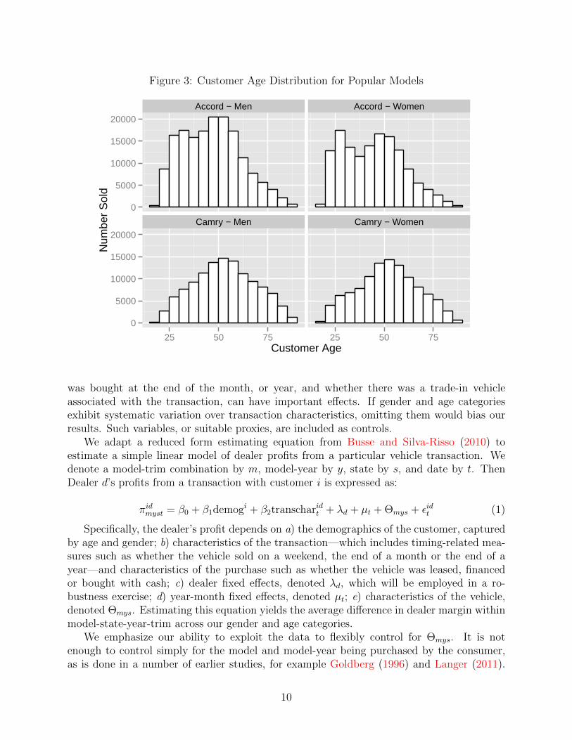
Figure 3: Customer Age Distribution for Popular Models

Accord − Men Accord − Women

Camry − Men Camry − Women

0

5000

10000

15000

20000

0

5000

10000

15000

20000

25 50 75 25 50 75Customer Age

Num

ber

Sol

d

was bought at the end of the month, or year, and whether there was a trade-in vehicleassociated with the transaction, can have important effects. If gender and age categoriesexhibit systematic variation over transaction characteristics, omitting them would bias ourresults. Such variables, or suitable proxies, are included as controls.

We adapt a reduced form estimating equation from Busse and Silva-Risso (2010) toestimate a simple linear model of dealer profits from a particular vehicle transaction. Wedenote a model-trim combination by m, model-year by y, state by s, and date by t. ThenDealer d’s profits from a transaction with customer i is expressed as:

πidmyst = β0 + β1demogi + β2transcharidt + λd + µt + Θmys + εidt (1)

Specifically, the dealer’s profit depends on a) the demographics of the customer, capturedby age and gender; b) characteristics of the transaction—which includes timing-related mea-sures such as whether the vehicle sold on a weekend, the end of a month or the end of ayear—and characteristics of the purchase such as whether the vehicle was leased, financedor bought with cash; c) dealer fixed effects, denoted λd, which will be employed in a ro-bustness exercise; d) year-month fixed effects, denoted µt; e) characteristics of the vehicle,denoted Θmys. Estimating this equation yields the average difference in dealer margin withinmodel-state-year-trim across our gender and age categories.

We emphasize our ability to exploit the data to flexibly control for Θmys. It is notenough to control simply for the model and model-year being purchased by the consumer,as is done in a number of earlier studies, for example Goldberg (1996) and Langer (2011).

10

This is because, even within a given model, customers can choose different trims in a mannerthat may be correlated with their demographics.15 But even controlling for the model andtrim, as has been done in other studies, for example Harless and Hoffer (2002), may not beenough. This is partly because there may be other options that consumers purchase, whichwe capture by examining dealer margins, but also because prices or margins for a givenmodel-trim combination are likely to vary across markets due to differences in consumerdemand or the network of dealers.

To address all of these possible issues we control in our regressions for the combination ofa model, model-year, trim and the state of purchase, and estimate demographic differenceswithin these combinations. As a concrete example, we compare consumers purchasing a 2007Honda Civic LX in California with other consumers purchasing exactly the same vehicle inthe same state, while also accounting for unobserved options in each purchase. In additionalrobustness checks we include fixed-effects for the city and state in which the purchaserresides. No prior study of demographics in new car sales has accounted for such a fine level ofvariation across transactions. We argue that, once all of these features of various transactionsare accounted for, differences in dealer margins must emerge from the negotiation processrather than from different vehicle choices by consumers, as we discuss in more detail below.

4 Results

We now present our results. This section is divided into four parts. We first documentthe extent of variation in new car prices, showing that there are huge differences in finalprices paid for the same new car, even after controlling for all observable characteristics ofthe transaction. Next, we show that the demographics of consumers explain a significantportion of these differences. We then show that these results do not change in response to awide variety of robustness checks. Finally, we extend our results to the Canadian market.

4.1 Variation in Dealer Margins

In this subsection we establish that there is huge variation in negotiated prices for newvehicles. Differences in the final prices for the same new car model can be many hundredsof dollars, even accounting for all observable aspects of the transaction.

We emphasize again that our main variable of interest is the dealer’s margin on the newcar, which is recorded as the difference between the purchase price and the dealer’s invoiceprice, for reasons discussed in Section 3. In Table 3, we summarize two measures of dispersionin dealer margins. We focus on the difference between the 90th and 10th percentiles of thedealer margin distribution, as well as between the 75th and 25th percentiles. Examiningthese percentiles allows us to consistently measure and compare the dispersion in pricespaid across various subsamples of the data, while also ignoring outlier observations that candistort such comparisons.

The first line of the Table shows these measures of dispersion for the full sample of almost10 million observations. The difference in dealer margins between the 90th and 10th per-

15Indeed, we will show later that this is precisely the case, as women tend to buy not just cheaper modelsthan men, but also cheaper trims within a given model.

11

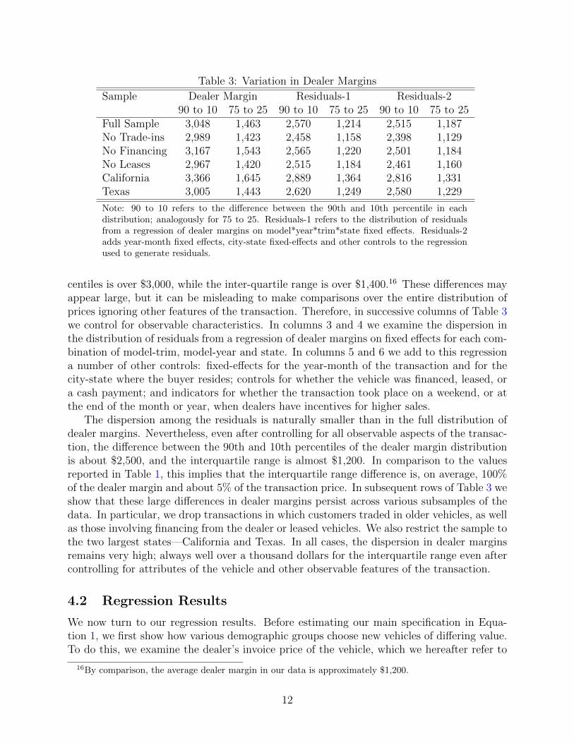
Table 3: Variation in Dealer Margins

Sample Dealer Margin Residuals-1 Residuals-290 to 10 75 to 25 90 to 10 75 to 25 90 to 10 75 to 25

Full Sample 3,048 1,463 2,570 1,214 2,515 1,187No Trade-ins 2,989 1,423 2,458 1,158 2,398 1,129No Financing 3,167 1,543 2,565 1,220 2,501 1,184No Leases 2,967 1,420 2,515 1,184 2,461 1,160California 3,366 1,645 2,889 1,364 2,816 1,331Texas 3,005 1,443 2,620 1,249 2,580 1,229

Note: 90 to 10 refers to the difference between the 90th and 10th percentile in eachdistribution; analogously for 75 to 25. Residuals-1 refers to the distribution of residualsfrom a regression of dealer margins on model*year*trim*state fixed effects. Residuals-2adds year-month fixed effects, city-state fixed-effects and other controls to the regressionused to generate residuals.

centiles is over $3,000, while the inter-quartile range is over $1,400.16 These differences mayappear large, but it can be misleading to make comparisons over the entire distribution ofprices ignoring other features of the transaction. Therefore, in successive columns of Table 3we control for observable characteristics. In columns 3 and 4 we examine the dispersion inthe distribution of residuals from a regression of dealer margins on fixed effects for each com-bination of model-trim, model-year and state. In columns 5 and 6 we add to this regressiona number of other controls: fixed-effects for the year-month of the transaction and for thecity-state where the buyer resides; controls for whether the vehicle was financed, leased, ora cash payment; and indicators for whether the transaction took place on a weekend, or atthe end of the month or year, when dealers have incentives for higher sales.

The dispersion among the residuals is naturally smaller than in the full distribution ofdealer margins. Nevertheless, even after controlling for all observable aspects of the transac-tion, the difference between the 90th and 10th percentiles of the dealer margin distributionis about $2,500, and the interquartile range is almost $1,200. In comparison to the valuesreported in Table 1, this implies that the interquartile range difference is, on average, 100%of the dealer margin and about 5% of the transaction price. In subsequent rows of Table 3 weshow that these large differences in dealer margins persist across various subsamples of thedata. In particular, we drop transactions in which customers traded in older vehicles, as wellas those involving financing from the dealer or leased vehicles. We also restrict the sample tothe two largest states—California and Texas. In all cases, the dispersion in dealer marginsremains very high; always well over a thousand dollars for the interquartile range even aftercontrolling for attributes of the vehicle and other observable features of the transaction.

4.2 Regression Results

We now turn to our regression results. Before estimating our main specification in Equa-tion 1, we first show how various demographic groups choose new vehicles of differing value.To do this, we examine the dealer’s invoice price of the vehicle, which we hereafter refer to

16By comparison, the average dealer margin in our data is approximately $1,200.

12

as the vehicle cost. The vehicle cost is determined in advance of the transaction and so doesnot reflect any elements of the negotiating process. Therefore, differences in vehicle costsacross demographic groups must purely reflect different choices by consumers.

Table 4 presents the results from regressing the log of the vehicle cost in each transactionon demographic characteristics and other controls. The omitted demographic group is maleconsumers under the age of 25. In column 1 we control simply for the state in whichthe transaction took place, as well as year*month fixed effects. The results show that thecheapest vehicles are bought by women under 25, who pay about 8% less than men of thesame age. The most expensive vehicles are purchased by 35–40 year old men who pay 20%more than the omitted category.

Differences in vehicle costs can be driven either by the consumer’s choice of model, orby the choice of more expensive trims within a model. Therefore, in column 2 we controlfor the combination of state, model and model-year. This naturally produces much smallerdifferences, since any variation now must be driven almost entirely by the choice of vehicletrim. Nevertheless, we see a significant relationship between gender and the choice of trim.Within a given model, women appear to consistently buy cheaper trims than men of the sameage; the difference is, on average, about 0.7% of the cost of the vehicle, which is statisticallysignificant in almost all age groups, and which translates to about $200 on average. Incolumn 3 we estimate fixed-effects for the interaction of state, model, model-year and trim.Differences between the genders now are tiny and generally not significant. Any remainingdifferences must be due to consumers’ choice of accessories and aftermarket options, whichwill be controlled for in our regressions of dealer margin.

These results suggest that there are clear gender differences in the choice of models, aswell as trims within a model, which are important to control for in order to credibly establishdifferences in negotiating patterns across demographic groups, which is what we turn to nowin our estimation of Equation 1.

Table 5 presents results from a set of regressions where the dependent variable is thedealer’s margin on each transaction and the main regressors of interest are the age andgender of consumers.17 The omitted age group is male consumers below 25. Column 1includes fixed-effects for the State of the transaction, Column 2 uses model*model-year*statefixed-effects, and Column 3 uses model*model-year*trim*state fixed-effects. All regressionsalso include year*month fixed-effects to control for general trends in vehicle costs and prices.Standard errors are clustered by model*model-year.

The results in the first column show that dealers, on average, make $137 less from femaleconsumers under the age of 25 than from male consumers of the same age. Male consumersbetween 60 and 65 years generate approximately $200 more in margins than the omittedgroup of male consumers under 25, and about $340 more than female consumers under 25.

Note, however, that since Column 1 does not control for the make, model or trim of thevehicle, the results for different age and gender groups may be driven by the types of cars theypurchase. For example, if young, female consumers tend to buy cheaper models or trims, andif dealers make lower margins on cheaper cars, then the results may just reflect these choices

17We do not transform the dealer margin by taking a log, as this would require dropping observationswhere margins are negative. Later, we show that our results are robust to using only transactions withpositive dealer margins and expressing the dependent variable in logs.

13

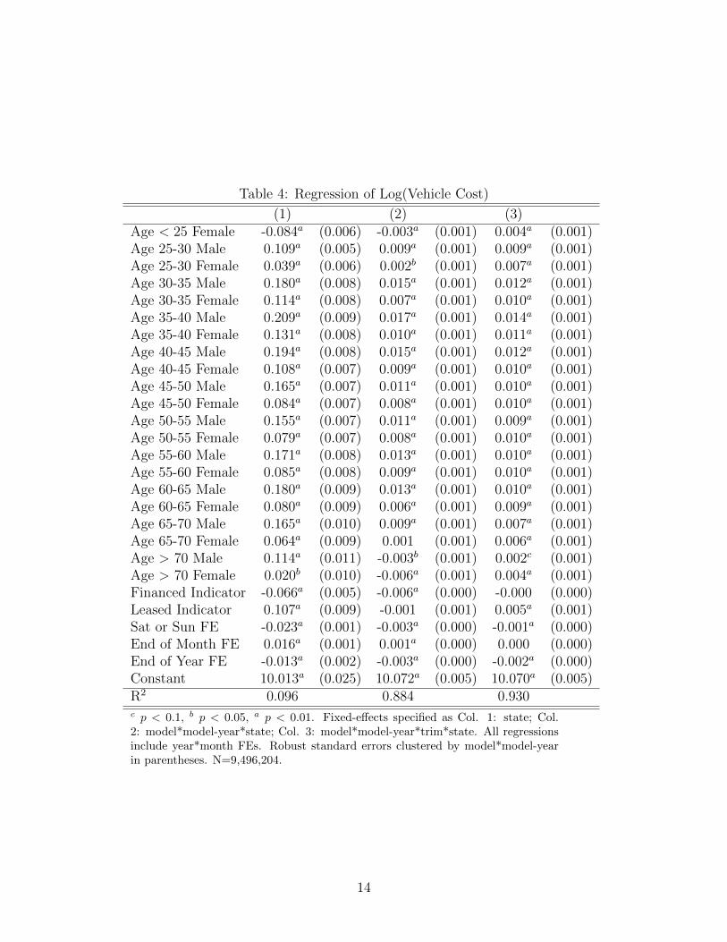
Table 4: Regression of Log(Vehicle Cost)

(1) (2) (3)Age < 25 Female -0.084a (0.006) -0.003a (0.001) 0.004a (0.001)Age 25-30 Male 0.109a (0.005) 0.009a (0.001) 0.009a (0.001)Age 25-30 Female 0.039a (0.006) 0.002b (0.001) 0.007a (0.001)Age 30-35 Male 0.180a (0.008) 0.015a (0.001) 0.012a (0.001)Age 30-35 Female 0.114a (0.008) 0.007a (0.001) 0.010a (0.001)Age 35-40 Male 0.209a (0.009) 0.017a (0.001) 0.014a (0.001)Age 35-40 Female 0.131a (0.008) 0.010a (0.001) 0.011a (0.001)Age 40-45 Male 0.194a (0.008) 0.015a (0.001) 0.012a (0.001)Age 40-45 Female 0.108a (0.007) 0.009a (0.001) 0.010a (0.001)Age 45-50 Male 0.165a (0.007) 0.011a (0.001) 0.010a (0.001)Age 45-50 Female 0.084a (0.007) 0.008a (0.001) 0.010a (0.001)Age 50-55 Male 0.155a (0.007) 0.011a (0.001) 0.009a (0.001)Age 50-55 Female 0.079a (0.007) 0.008a (0.001) 0.010a (0.001)Age 55-60 Male 0.171a (0.008) 0.013a (0.001) 0.010a (0.001)Age 55-60 Female 0.085a (0.008) 0.009a (0.001) 0.010a (0.001)Age 60-65 Male 0.180a (0.009) 0.013a (0.001) 0.010a (0.001)Age 60-65 Female 0.080a (0.009) 0.006a (0.001) 0.009a (0.001)Age 65-70 Male 0.165a (0.010) 0.009a (0.001) 0.007a (0.001)Age 65-70 Female 0.064a (0.009) 0.001 (0.001) 0.006a (0.001)Age > 70 Male 0.114a (0.011) -0.003b (0.001) 0.002c (0.001)Age > 70 Female 0.020b (0.010) -0.006a (0.001) 0.004a (0.001)Financed Indicator -0.066a (0.005) -0.006a (0.000) -0.000 (0.000)Leased Indicator 0.107a (0.009) -0.001 (0.001) 0.005a (0.001)Sat or Sun FE -0.023a (0.001) -0.003a (0.000) -0.001a (0.000)End of Month FE 0.016a (0.001) 0.001a (0.000) 0.000 (0.000)End of Year FE -0.013a (0.002) -0.003a (0.000) -0.002a (0.000)Constant 10.013a (0.025) 10.072a (0.005) 10.070a (0.005)R2 0.096 0.884 0.930c p < 0.1, b p < 0.05, a p < 0.01. Fixed-effects specified as Col. 1: state; Col.2: model*model-year*state; Col. 3: model*model-year*trim*state. All regressionsinclude year*month FEs. Robust standard errors clustered by model*model-yearin parentheses. N=9,496,204.

14

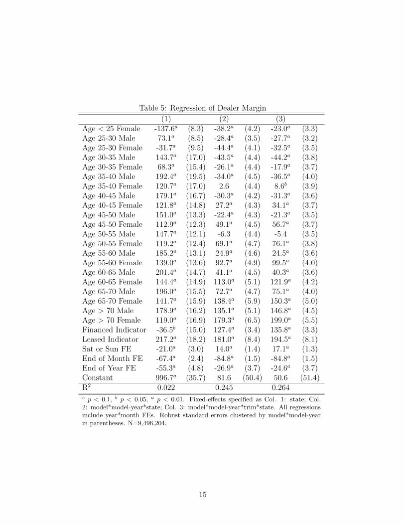
Table 5: Regression of Dealer Margin

(1) (2) (3)Age < 25 Female -137.6a (8.3) -38.2a (4.2) -23.0a (3.3)Age 25-30 Male 73.1a (8.5) -28.4a (3.5) -27.7a (3.2)Age 25-30 Female -31.7a (9.5) -44.4a (4.1) -32.5a (3.5)Age 30-35 Male 143.7a (17.0) -43.5a (4.4) -44.2a (3.8)Age 30-35 Female 68.3a (15.4) -26.1a (4.4) -17.9a (3.7)Age 35-40 Male 192.4a (19.5) -34.0a (4.5) -36.5a (4.0)Age 35-40 Female 120.7a (17.0) 2.6 (4.4) 8.6b (3.9)Age 40-45 Male 179.1a (16.7) -30.3a (4.2) -31.3a (3.6)Age 40-45 Female 121.8a (14.8) 27.2a (4.3) 34.1a (3.7)Age 45-50 Male 151.0a (13.3) -22.4a (4.3) -21.3a (3.5)Age 45-50 Female 112.9a (12.3) 49.1a (4.5) 56.7a (3.7)Age 50-55 Male 147.7a (12.1) -6.3 (4.4) -5.4 (3.5)Age 50-55 Female 119.2a (12.4) 69.1a (4.7) 76.1a (3.8)Age 55-60 Male 185.2a (13.1) 24.9a (4.6) 24.5a (3.6)Age 55-60 Female 139.0a (13.6) 92.7a (4.9) 99.5a (4.0)Age 60-65 Male 201.4a (14.7) 41.1a (4.5) 40.3a (3.6)Age 60-65 Female 144.4a (14.9) 113.0a (5.1) 121.9a (4.2)Age 65-70 Male 196.0a (15.5) 72.7a (4.7) 75.1a (4.0)Age 65-70 Female 141.7a (15.9) 138.4a (5.9) 150.3a (5.0)Age > 70 Male 178.9a (16.2) 135.1a (5.1) 146.8a (4.5)Age > 70 Female 119.0a (16.9) 179.3a (6.5) 199.0a (5.5)Financed Indicator -36.5b (15.0) 127.4a (3.4) 135.8a (3.3)Leased Indicator 217.2a (18.2) 181.0a (8.4) 194.5a (8.1)Sat or Sun FE -21.0a (3.0) 14.0a (1.4) 17.1a (1.3)End of Month FE -67.4a (2.4) -84.8a (1.5) -84.8a (1.5)End of Year FE -55.3a (4.8) -26.9a (3.7) -24.6a (3.7)Constant 996.7a (35.7) 81.6 (50.4) 50.6 (51.4)R2 0.022 0.245 0.264c p < 0.1, b p < 0.05, a p < 0.01. Fixed-effects specified as Col. 1: state; Col.2: model*model-year*state; Col. 3: model*model-year*trim*state. All regressionsinclude year*month FEs. Robust standard errors clustered by model*model-yearin parentheses. N=9,496,204.

15

Figure 4: Dealer Margin across demographic groups, relative to Men under 25

0

100

200

<25 25−30 30−35 35−40 40−45 45−50 50−55 55−60 60−65 65−70 70+Age Group

Dea

ler

Mar

gin

Gender

female

male

rather than differences in negotiation. Therefore, in column 2 of Table 5, we estimate thesame relationship as before, but we include model*model-year*state fixed-effects. We nowfind that there appears to be a clear age premium in new car negotiations—the youngestconsumers pay considerably less than older consumers for identical vehicles. We also findthat, with the exception of the youngest age category of consumers under 25, men negotiatelower prices on average than women of the same age. These differences are small at first,but grow steadily among older consumers. In column 3, we estimate this relationship withina vehicle’s model-trim. We find that the differences persist, and are in fact somewhat largeramong older consumers.

Thus, not only does the premium paid by consumers rise with age, but it does so muchmore steeply for women than for men. We illustrate this in Figure 4, by plotting the coeffi-cient estimates from Column 3 of Table 5. The shaded regions around each plot are the 95%confidence intervals. F-tests indicate that the coefficients for men and women of the sameage are almost always significantly different from each other at the 1% level. (The exceptionis the 25-30 age group.)

According to the coefficients from column 3, dealer margins are the lowest for 30–35 yearold men, who pay $36 less than the omitted category of men under 25, and highest for women

16

over 70 who overpay by $200. Therefore, there is a $236 difference, on average, between thehighest and lowest paying demographic groups. The average dealer margin earned across allvehicles in our data is $1,215 (see Table 1). Thus, the oldest women generate a margin thatis almost 20% higher than the lowest paying consumers who buy the same vehicle.

Turning to the other factors that may influence dealer margins, we see from the thirdcolumn in Tables 5 that dealers make $135–195 higher margins on cars that are leased orfinanced, relative to outright cash purchases. This accords with common observations aboutthe new car market. Finally, dealers clearly earn lower margins at the end of the month andyear. On average, their margins are lower by $85 and $109 (the sum of the end-of-monthand end-of-year coefficients) at these times, again conforming to casual observations, andconfirming that dealers respond to manufacturer incentives at the end of calendar monthsand years. Note that these lower margins may be caused either by dealers being willingto sacrifice profits to meet sales quotas, or by more price-conscious consumers choosing topurchase cars at these times, knowing the incentives that dealers face.

4.3 Robustness

In this section we show that our results are not driven by omitted variables, outlier observa-tions, or selection. We present the main coefficients of interest graphically in Figures 5 and 6.In each figure, the solid blue line represents dealer margins on female customers relative tomen under 25, while the dashed red line corresponds to margins on male customers. Theseresults are obtained from regressions using the same specification as Column 3 of Table 5,which include fixed effects for model-year-province-trim and for year-months.18

We start by examining particular segments—Compact cars and SUVs in Panels A andB of Figure 5. These segments are disproportionately associated with certain age groups;younger consumers are more likely to purchase small cars, while middle-aged consumers,especially those who are married, are more likely to purchase family cars such as SUVs. Wethen examine domestic (North American) and foreign manufacturers separately in panels Cand D. Anecdotal reports suggest that dealers of foreign cars are less likely to negotiate onfinal prices; if so, this may affect our results if demographic groups differ in their propensityto purchase foreign cars.

In Panel E of Figure 5 we include dealer profits from service contracts in our definitionof dealer margins. Our data indicate that these service contracts are disproportionatelylikely to be purchased by older buyers, and therefore may affect negotiated prices and therecorded dealer margin if dealers are willing to sacrifice profits on the new car sale, expectingto make these up on the sale of service contracts.19 Note, though, that such behavior wouldstrengthen our earlier results.

We then show, in Panel F, that our results are robust to examining popular car modelsalone; this is to verify that are results are not driven by unusual consumer or dealer behaviorin vehicles with low sales. We define high-selling car models as those with at least 50,000

18We do not present confidence intervals in these figures to avoid crowding. Regression results, and thefull set of clustered standard errors for these exercises, are presented in Tables 10, 11, 12 and 13 in the onlineappendix.

19Sallee (2011) cites the purchasing of a service contracts as evidence that a car buyer is less savvy.

17

Figure 5: Dealer Margins for subsamples, by Gender and Age

A: Compacts B: SUVs C: Domestic

D: Foreign E: Service Contracts F: High Selling

0

100

200

0

100

200

25−30 40−45 55−60 70+ 25−30 40−45 55−60 70+ 25−30 40−45 55−60 70+Age Group

Dea

ler

Mar

gin

Gender

female

male

Figure 6: Dealer Margins for subsamples, by Gender and Age

A: No Trade−ins B: No Financing C: No Leases

D: California E: Texas F: Florida−100

0

100

200

−100

0

100

200

25−30 40−45 55−60 70+ 25−30 40−45 55−60 70+ 25−30 40−45 55−60 70+Age Group

Dea

ler

Mar

gin

Gender

female

male

18

units sold during our sample period. This limits our sample to 53 models, out of an initialset of more than 600 models, but they comprise around 56% of total sales.

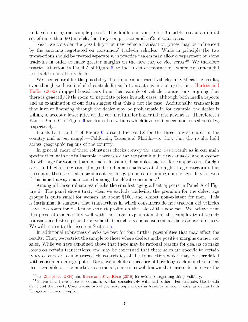
Next, we consider the possibility that new vehicle transaction prices may be influencedby the amounts negotiated on consumers’ trade-in vehicles. While in principle the twotransactions should be treated separately, in practice dealers may allow overpayment on sometrade-ins in order to make greater margins on the new car, or vice versa.20 We thereforerestrict attention, in Panel A of Figure 6, to the subset of transactions where consumers didnot trade-in an older vehicle.

We then control for the possibility that financed or leased vehicles may affect the results,even though we have included controls for such transactions in our regressions. Harless andHoffer (2002) dropped leased cars from their sample of vehicle transactions, arguing thatthere is generally little room to negotiate prices in such cases, although both media reportsand an examination of our data suggest that this is not the case. Additionally, transactionsthat involve financing through the dealer may be problematic if, for example, the dealer iswilling to accept a lower price on the car in return for higher interest payments. Therefore, inPanels B and C of Figure 6 we drop observations which involve financed and leased vehicles,respectively.

Panels D, E and F of Figure 6 present the results for the three largest states in thecountry and in our sample—California, Texas and Florida—to show that the results holdacross geographic regions of the country.

In general, most of these robustness checks convey the same basic result as in our mainspecification with the full sample: there is a clear age premium in new car sales, and a steeperrise with age for women than for men. In some sub-samples, such as for compact cars, foreigncars, and high-selling cars, the gender difference narrows at the highest age categories, butit remains the case that a significant gender gap opens up among middle-aged buyers evenif this is not always maintained among the oldest consumers.21

Among all these robustness checks the smallest age-gradient appears in Panel A of Fig-ure 6. The panel shows that, when we exclude trade-ins, the premium for the oldest agegroups is quite small for women, at about $100, and almost non-existent for men. Thisis intriguing; it suggests that transactions in which consumers do not trade-in old vehiclesleave less room for dealers to extract profits on the sale of the new car. We believe thatthis piece of evidence fits well with the larger explanation that the complexity of vehicletransactions fosters price dispersion that benefits some consumers at the expense of others.We will return to this issue in Section 5.

In additional robustness checks we test for four further possibilities that may affect theresults. First, we restrict the sample to those where dealers make positive margins on new carsales. While we have explained above that there may be rational reasons for dealers to makelosses on certain transactions, one may be concerned that these sales are specific to certaintypes of cars or to unobserved characteristics of the transaction which may be correlatedwith consumer demographics. Next, we include a measure of how long each model-year hasbeen available on the market as a control, since it is well known that prices decline over the

20See Zhu et al. (2008) and Busse and Silva-Risso (2010) for evidence regarding this possibility.21Notice that these three sub-samples overlap considerably with each other. For example, the Honda

Civic and the Toyota Corolla were two of the most popular cars in America in recent years, as well as bothforeign-owned and compact.

19

course of a model-cycle, and demographic groups may vary in their propensity to purchasevehicles over their model-cycles. Next, we include as a regressor the number of days thatthe vehicle has been on the dealer’s lot—popular cars typically turnover very quickly and sodealers may be willing to reduce margins on cars that are not in high demand. Finally, weinclude fixed-effects for the city and state in which the purchaser resides, to control for finemarket-level differences in demand or supply that may not be captured by state fixed-effects,especially in large states.22 The results, which are reported in the appendix, in all four casesare very similar to our main results.

4.4 Extension to the Canadian market

We briefly show in this section that our results are similar when extended to the Canadianmarket. The automobile industries in Canada and the U.S. are closely integrated, andthe North American manufacturers, in particular, operate production on both sides of theborder. All of the major domestic and foreign manufacturers offer the same set of vehiclesin both countries, albeit with occasional differences in the names of car models, and minordifferences in specifications. The process of customer negotiation for new cars is also almostidentical in the U.S. and Canada.

Our data provider gave us access to a sample of approximately 1 million new car transac-tions in Canada. Most of the relevant variables are identical to those in the U.S. sample. Oneadditional variable contained in the Canadian data is an identifier for the dealer at whichthe vehicle was purchased. As a result we can examine whether including dealer fixed-effectshas any effect on the results. In the U.S. data used above, the most we could include in thisregard was the geographic location of the consumer, which effectively controlled for regionalvariation in final prices, but did not allow for systematic differences in the behaviour of in-dividual car dealers. This may be a concern if, for example, dealers located in smaller citiesor suburban locations charge lower prices for exactly the same car as a city dealer who faceshigher costs. If the demographic distribution of consumers in these two locations is alsodifferent—for example, if older consumers are more likely to live near high-cost dealers—then this selection of consumer types may drive our results. We control for this possibility byincluding dealer fixed-effects in the Canadian sample, which allow us to look within dealers.

Figure 7 presents the coefficients from running our main regression specification on thesample of Canadian auto transactions.23 The left panel shows the main regression whilethe right panel adds dealer fixed-effects. There are two main points of interest. First,the results we obtained for the United States hold broadly in Canada as well. One clearexception appears to be that young, female consumers in Canada outperform their malecounterparts. However, the two main results from the US sample—that there appears tobe an age premium, and that this premium rises more steeply with age for women than formen—continue to hold in the Canadian market.

The second point of interest is that adding dealer fixed-effects has virtually no effecton the estimated age and gender effects. This is visually apparent from Figure 7, and ths

22This is computationally very intensive as there are over 50,000 individual city-state combinations in thedata. For this exercise we restricted the sample to the 75% of observations accounted for by larger townsand cities.

23The full regression results are in the online appendix.

20

Figure 7: Dealer Margins for subsamples, by Gender and Age: Canadian Data

A: Canada B: Canada, Dealer FEs

−100

−50

0

50

100

25−30 40−45 55−60 70+ 25−30 40−45 55−60 70+Age Group

Dea

ler

Mar

gin

Gender

female

male

conclusion holds up when examining the coefficients in detail. This suggests that the resultsin our main sample using US data are not driven by systematic differences in dealer behavior.

4.5 Summary

We emphasize three findings emerging from our results—see Figures 4, 5, 6 and 7. a) There isconsiderable variation in the prices paid for new cars, even after controlling for all observablefeatures of the transaction—the difference between the 75th and 25th percentiles of thedistribution of dealer margin residuals is well over a thousand dollars (compared to theaverage dealer margin of $1,215). b) There appears to be a clear age premium in new carsales, with older consumers paying significantly more than younger consumers for the samevehicle, and a steady, almost monotonic, increase in margins with age. c) There also appearsto be a gender divide that increases with age; as a result, older women pay the most among allconsumers for a given vehicle, which is about $240 more than the lowest paying consumers.

These results are interesting and perhaps also surprising. We control for the combinationof model, state and trim of each vehicle. We also control for the timing of the transaction, thelocation of the buyer (through the state of residence, but also the city in a robustness check),and the dealer’s cost of the purchased vehicle. We come very close to examining differences indealer margins for identical products sold at the same time to different consumers. Therefore,any remaining differences in dealer margins beyond these controls must derive purely fromidiosyncratic differences between customers. We further show that average differences acrossage and gender groups account for around 20% of the remaining variation. We now turn tothe question of why consumer demographics should affect the negotiating process.

21

5 Discussion of the Results

In this section we discuss potential explanations for our findings. We first address the concernthat our results may not accurately reflect outcomes for the gender and age group associatedwith each transaction. In particular, one may be concerned that the person negotiating forthe car is not always the same as the primary buyer listed on the invoice, and that thismay be particularly likely for women and younger consumers, who may be accompanied byfriends or family members negotiating on their behalf.24 However, third person negotiationis unlikely to explain our pattern of results. Younger consumers—both men and women—generally obtain the best negotiating outcomes. If these consumers are helped in bargainingby their fathers, for example, it would be strange that these men do a better job negotiatingfor their children than for themselves. On the other hand, if we believe that a fraction ofcars sold to women involve negotiations by male partners, our results will understate thetrue gender differences in negotiation. In that case, women on their own are likely to doeven worse than our results indicate.

Similarly there may be sample selection driven by marriage—women are perhaps lesslikely to be listed as the primary buyer on “family cars” bought jointly with their husbands.If this selection removes superior female negotiators from our sample, our results will notrepresent the entire female population.25 However, the sample selection explanation requiresnot just that married women are less likely to be listed as the primary buyer, but also that thisproportion increases with age. In addition, it requires the sample of women purchasing carsby themselves (potentially single) to be worse negotiators, on average, than married womenjointly negotiating with their partners. These possibilities cannot be ruled out, but theyrequire unlikely conditions. We see no clear reason why single older women would inherentlybe worse negotiators than women of the same age who are married or in a relationship.26

Further, if this were in fact true, it would imply that the results would be different for thosesegments that comprise a high proportion of family cars. Recall, however, that our resultswere no different for SUVs—which are typical family cars—than for our full sample. We alsofind similar results for the Van segment, see Table 10 in the Appendix.

In our dataset the proportion of female buyers falls with customer age—see Panel A inFigure 8—partially supporting the view that older married women are less likely to be listedas the primary buyer. However, in panel B of the same figure we illustrate the likelihood ofbeing married, by age group, for females in the United States in 2005. The probability thata woman is married crosses 60% by her mid-thirties and then begins to decline after age 45,falling quite sharply after age 60, due to the effects of both divorce and bereavement. Thus,women in their 60s or older are significantly less likely to be married than women in their30s and 40s, suggesting that the marriage-based explanation does not influence our results.

Thus, we believe it is unlikely that our results are driven by selection—i.e. by the removalof better negotiators from the cohort of older women in our sample. Instead, our results maybe consistent with causality running in the opposite direction: the worse performance ofolder women in new car negotiations may lead some of them to drop out of the market

24See Goldberg (1996) for a discussion of this issue.25See Langer (2011) for a detailed discussion related to this issue.26Census data indicate that unmarried women in the 40–60 age group are more likely to participate in the

labor force than married women, and that the two groups have similar levels of educational attainment.

22

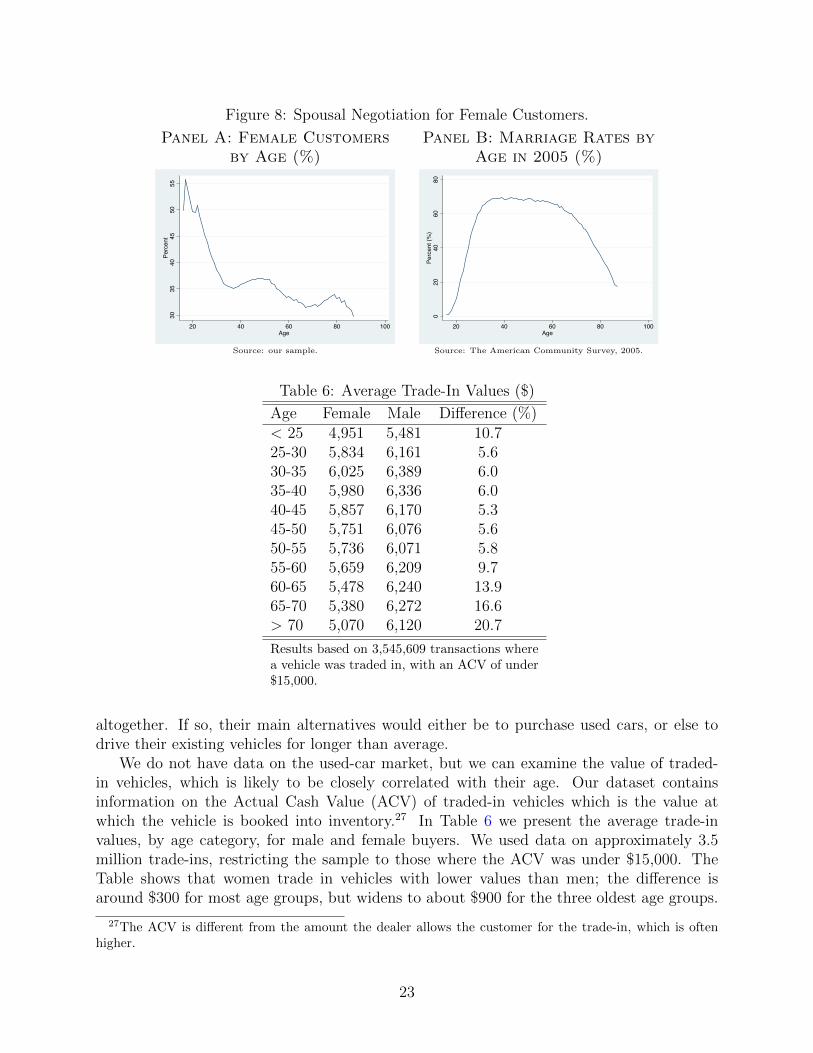
Figure 8: Spousal Negotiation for Female Customers.

Panel A: Female Customersby Age (%)

3035

4045

5055

Percent

20 40 60 80 100Age

Source: our sample.

Panel B: Marriage Rates byAge in 2005 (%)

020

4060

80Pe

rcen

t (%

)

20 40 60 80 100Age

Source: The American Community Survey, 2005.

Table 6: Average Trade-In Values ($)

Age Female Male Difference (%)< 25 4,951 5,481 10.725-30 5,834 6,161 5.630-35 6,025 6,389 6.035-40 5,980 6,336 6.040-45 5,857 6,170 5.345-50 5,751 6,076 5.650-55 5,736 6,071 5.855-60 5,659 6,209 9.760-65 5,478 6,240 13.965-70 5,380 6,272 16.6> 70 5,070 6,120 20.7

Results based on 3,545,609 transactions wherea vehicle was traded in, with an ACV of under$15,000.

altogether. If so, their main alternatives would either be to purchase used cars, or else todrive their existing vehicles for longer than average.

We do not have data on the used-car market, but we can examine the value of traded-in vehicles, which is likely to be closely correlated with their age. Our dataset containsinformation on the Actual Cash Value (ACV) of traded-in vehicles which is the value atwhich the vehicle is booked into inventory.27 In Table 6 we present the average trade-invalues, by age category, for male and female buyers. We used data on approximately 3.5million trade-ins, restricting the sample to those where the ACV was under $15,000. TheTable shows that women trade in vehicles with lower values than men; the difference isaround $300 for most age groups, but widens to about $900 for the three oldest age groups.

27The ACV is different from the amount the dealer allows the customer for the trade-in, which is oftenhigher.

23

Proportionately, the average gender difference in trade-in values is 5–6% for consumers underage 55, but over 20% for those above 70. Clearly, older women trade in lower valued carsthan younger women, relative to men of the same age. One possible explanation is that olderwomen drive their cars for longer before trading them in, which explains, at least in part,our earlier finding that women are less represented among older cohorts of car buyers.

Our results therefore suggest the possibility that we raised early on in this paper—thatloss aversion or perceived differences in negotiating ability may cause some demographicgroups to avoid markets that involve negotiation.

We now turn to explanations for our results. Any comprehensive explanation of our re-sults should account for both the age and gender-related patterns documented. There is alarge literature on gender differences in negotiations, primarily over wages, and some consen-sus that women perform worse in such negotiations either due to discrimination or their ownreluctance to negotiate; see Babcock and Laschever (2003), List (2004) and Leibbrandt andList (2012). In the new car market itself, Ayres and Siegelman (1995) famously showed thatwomen were initially offered worse terms, although these results were later contested. How-ever, our findings argue against systematic discrimination against women, primarily becausethere is clear evidence that among younger cohorts women perform no worse than men, andpossibly even a little better.

Analogously, there may be reasons that older consumers perform worse in negotiations.Prior research has shown that older consumers are less likely to try new brands or products;see Lambert-Pandraud and Laurent (2010). More relevant to our study, Lambert-Pandraudet al. (2005) find evidence in the new car market that older customers are more likely topurchase the same brand as their existing vehicle. They also consider fewer brands, fewerdealers, and fewer models than younger customers. Such an attachment to brands canallow dealers to extract higher profits from older customers. Both these studies offer severalexplanations for age related brand attachment including: change aversion, cognitive decline,and even nostalgia. While this is a relevant explanation for our findings, it does not fullyexplain the gender based differences that we observe.

A plausible explanation for our results may lie in differences in search and negotiationcosts across various demographic groups. Morton et al. (2011) show that search costs and in-complete information have an important effect on negotiations, particularly that consumerswith information of dealers’ reservation prices capture larger shares from their margin. Thisis more important with access to the Internet, as online car referral services such as Ed-munds.com often reveal dealer costs. If certain consumers are less likely to access the Inter-net for research, their higher search and negotiating costs could lead to poorer negotiations.Goldfarb and Prince (2008) document the digital divide in Internet use, showing that womenand older consumers are less likely to use the Internet, controlling for other factors (they donot interact age and gender). In Panel A of Figure 9 we present the fraction of the popula-tion accessing the Internet from any location by sex and age in 2007. Our data on Internetuse is from the Integrated Public Use Microdata Series of the Current Population Survey forthe USA (King et al., 2013).28 We find that older individuals in the US are markedly lesslikely to use the Internet, however the data do not indicate large differences across gender(females are represented by the solid line and males by the dashed line).

28We use the variable titled “person accesses the internet at any location,” from IPUMS-USA.

24

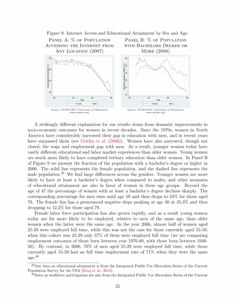
Figure 9: Internet Access and Educational Attainment by Sex and Age.

Panel A: % of PopulationAccessing the Internet from

Any Location (2007)20

4060

80U

sing

Inte

rnet

Any

whe

re (%

)

20 40 60 80Age

Female Male

Source: PUMS-CPS, University of Minnesota,www.ipums.org.

Panel B: % of Populationwith Bachelors Degree or

More (2006)

1015

2025

3035

Bach

elor

s D

egre

e or

Hig

her (

%)

20 40 60 80Age

Female Male

Source: PUMS-CPS, University of Minnesota,www.ipums.org.

A strikingly different explanation for our results stems from dramatic improvements insocio-economic outcomes for women in recent decades. Since the 1970s, women in NorthAmerica have considerably narrowed their gap in education with men, and in recent yearshave surpassed them (see Goldin et al. (2006)). Women have also narrowed, though notclosed, the wage and employment gap with men. As a result, younger women today havevastly different educational and labor market experiences than older women. Young womenare much more likely to have completed tertiary education than older women. In Panel Bof Figure 9 we present the fraction of the population with a bachelor’s degree or higher in2006. The solid line represents the female population, and the dashed line represents themale population.29 We find large differences across the genders. Younger women are morelikely to have at least a bachelor’s degree when compared to males, and other measuresof educational attainment are also in favor of women in these age groups. Beyond theage of 47 the percentage of women with at least a bachelor’s degree declines sharply. Thecorresponding percentage for men rises until age 59 and then drops to 24% for those aged79. The female line has a pronounced negative slope peaking at age 30 at 35.3% and thendropping to 12.2% for those aged 79.

Female labor force participation has also grown rapidly, and as a result young womentoday are far more likely to be employed, relative to men of the same age, than olderwomen when the latter were the same age. In the year 2006, almost half of women aged25-29 were employed full time, while this was not the case for those currently aged 55-59;when this cohort was 25-29 only 37% of them were employed full time (we are comparingemployment outcomes of those born between year 1976-80, with those born between 1946-50). By contrast, in 2006, 70% of men aged 25-29 were employed full time, while thosecurrently aged 55-59 had an full time employment rate of 71% when they were the sameage.30

29Our data on educational attainment is from the Integrated Public Use Microdata Series of the CurrentPopulation Survey for the USA (King et al., 2013).

30Data on workforce participation are also from the Integrated Public Use Microdata Series of the Current

25

Socio-economic trends in Canada have matched those in the US, with clear evidencethat women have dramatically improved their levels of educational attainment and alsonarrowed the gap in employment with men, over the last few decades. As a result, it isthe case in Canada, too, that older women today have lower levels of education and laborforce participation, relative to men, than women in their 20s. Therefore, these demographictrends may well explain the similar pattern of results that we established for the Canadianmarket.

Our results are consistent with the notion that the similar educational attainment andlabor force participation of young women, relative to men of the same age, allows them toperform as well in negotiations. Women above the age of 60 are much less likely to have com-pleted high-school or college, or to have been employed full-time when they were younger.These differences can potentially cause older women to have lower information in the new carmarket and perhaps also to negotiate with less confidence. This is likely to play an impor-tant role given the complexity of negotiations, which include discussions around financing,monthly payments, trade-in allowances and service contracts. Correspondingly, this may ex-plain why younger women of today are as good negotiators as their male counterparts. Notethat if this explanation is correct, it is unlikely that today’s cohort of younger women willdo worse than their male counterparts as they age. The difference in relationships observedis therefore likely to be specific to the cohorts currently observed, rather than reflecting anongoing effect.

We also performed a state-by-state analysis to examine whether these trends were par-ticularly apparent in US states or Canadian provinces that had the greatest or lowest socio-economic changes for women. These results were inconclusive, primarily because we neededto assign state-wide averages for educational attainment and labor force participation to oursample of buyers in each state. If we had microdata on education and employment for theconsumers in our sample, it is possible that we would have found more conclusive evidencein this regard.

Nevertheless, we do see some evidence that transactions with lower levels of complexityhave less dispersed prices and smaller age- and gender-related premiums. Recall, from Sec-tion 4, that the smallest age-gender gradient was obtained on the sub-sample of the datawhere customers did not trade-in an existing vehicle. Negotiations over the trade-in con-stitute an important part of the overall car buying process, along with discussions aboutother issues. Dealers, who perform many such negotiations, have considerably more expe-rience and information on these matters than consumers, and it is likely that they can usethe complexity of transactions to their advantage. For example, they may offer consumersseemingly attractive terms on the new car, only to make up the difference through a lowertrade-in allowance, higher interest rates, profitable service contracts, extended warranties,and other fees. It is revealing, therefore, that transactions that do not feature trade-insalso have smaller differences across demographic groups, suggesting that trade-in allowancesare one way for dealers to profit on less informed customers. This fits well with the largerexplanation that consumers with more information, which could be driven by better educa-tion or even simply by better access to information on the Internet, perform better in pricenegotiations.

Population Survey. We use the data from the question regarding work status during their last week.

26

Our results relate closely to those of Langer (2011), who studied the relative performanceof married and single men and women in the new car market.31 Our results complementher finding that single men generally pay more than single women, which is probably therelevant comparison since Langer argues that the opposite result for married consumers maybe driven by selection of the stronger negotiating spouse. We view our results as extendingthose in Langer (2011) since we can break down the gender based results by the age ofconsumers, in a manner that has not been done so far in the literature.

6 Conclusions

In this paper we examine price negotiations in the new car market, with an emphasis onhow age and gender characteristics relate to disparate outcomes. We began by establishinglarge variation in prices paid for almost identical new cars. We then demonstrate systematicdifferences in how consumers of each gender, and various age groups, perform in price ne-gotiations. In general, older consumers pay more for new cars, but the trend is particularlystark among older women. As a result, women above the age of 70 generate almost $250more in dealer margins—which is about 20% of the average dealer margin—than the lowestpaying customers, even after controlling for all observable aspects of the transaction. It isrevealing, therefore, that older women are also the least represented among new car buyers.Our results are robust to cutting the data in many ways, and to adding a large number ofcovariates.

We also see evidence that younger women do as well, or better, than men of their age in thenew vehicle market. This is concurrent with the reversal of the gender gap in education, andthe narrowing of the gender gap in employment and wages. It could be that the rapid increasein women’s education, as well as the improvement in their earnings and work experiencerelative to men, has given women better information and more confidence while conductingprice negotiations. Therefore it could also be that the improvements women have seen frommore advanced education and greater work opportunities are not restricted only to the labormarket. This has important implications for other markets involving negotiations, such asthe housing market.

The main limitation of drawing this conclusion is that our results are based on a cross-section of transactions, albeit one that employs a very large sample of consumers drawnfrom the entire range of the age distribution. Confirmation of our hypothesis that genderdifferences in negotiation are related to educational and labor force outcomes requires apanel that tracks cohorts over a much longer period and uses micro data on socio-economiccharacteristics. Since such data do not currently exist in the automobile industry, our findingsshould be regarded as suggestive until they can be confirmed in future research.

Irrespective of the reasons underlying our findings, further research on markets withnegotiated prices is important. The existence of a negotiated markup in the automobilesector is indicative of market power. One potential solution for reducing age and genderbased disadvantages is to address the source of this market power. If one of the reasons for

31There are also a number of important differences: Langer uses a structural model to predict optimalmarkups from transaction price data, whereas we use reduced-form techniques based on direct calculationof dealer margins.

27

disparate outcomes is the lack of information, increasing the flow of information and easeof its access will help. Establishing the existence of demographic-based disparities in othernegotiated price markets, and identifying reasons behind these, should be goals for futureresearch in this area.

References

Allen, J., R. Clark, and J.-F. Houde (2014). Search frictions and market power in negotiatedprice markets. Technical report, National Bureau of Economic Research.

Ayres, I. and P. Siegelman (1995, June). Race and gender discrimination in bargaining fora new car. American Economic Review 85 (3), 304–21.

Babcock, L. R. and S. Laschever (2003). Women Don’t Ask: Negotiation and the GenderDivide. Princeton University Press.

Bester, H. (1993). Bargaining versus price competition in markets with quality uncertainty.The American Economic Review , 278–288.

Busse, M. R., C. R. Knittel, and F. Zettelmeyer (2013). Are consumers myopic? evidencefrom new and used car purchases. The American Economic Review 103 (1), 220–256.

Busse, M. R. and J. M. Silva-Risso (2010). ”one discriminatory rent” or ”double jeopardy”:Multicomponent negotiation for new car purchases. The American Economic Review ,470–474.

Chen, Y., S. Yang, and Y. Zhao (2008). A simultaneous model of consumer brand choiceand negotiated price. Management science 54 (3), 538–549.

Goldberg, P. K. (1996, June). Dealer price discrimination in new car purchases: Evidencefrom the consumer expenditure survey. Journal of Political Economy 104 (3), 622–54.

Goldfarb, A. and J. Prince (2008). Internet adoption and usage patterns are different:Implications for the digital divide. Information Economics and Policy 20 (1), 2–15.

Goldin, C., L. F. Katz, and I. Kuziemko (2006). The homecoming of american college women:The reversal of the college gender gap. Journal of Economic Perspectives 20 (4), 133–156.

Gowrisankaran, G., A. Nevo, and R. Town (2013). Mergers when prices are negotiated:Evidence from the hospital industry. Technical report, National Bureau of EconomicResearch.

Grennan, M. (2013). Price discrimination and bargaining: Empirical evidence from medicaldevices. The American Economic Review 103 (1), 145–177.

Harding, J. P., S. S. Rosenthal, and C. Sirmans (2003). Estimating bargaining power in themarket for existing homes. Review of Economics and statistics 85 (1), 178–188.

28

Harless, D. W. and G. E. Hoffer (2002, March). Do women pay more for new vehicles?evidence from transaction price data. American Economic Review 92 (1), 270–279.

Jindal, P. and P. Newberry (2014). Price negotiations and bargaining costs.

King, M., S. Ruggles, J. T. Alexander, S. Flood, K. Genadek, M. B. Schroeder, B. Trampe,and R. Vick (2013). Integrated public use microdata series, current population survey:Version 3.0 [machine-readable database]. 2010. Minneapolis: University of Minnesota.

Lambert-Pandraud, R. and G. Laurent (2010). Why do older consumers buy older brands?the role of attachment and declining innovativeness. Journal of Marketing 74 (5), 104–121.

Lambert-Pandraud, R., G. Laurent, and E. Lapersonne (2005). Repeat purchasing of newautomobiles by older consumers: empirical evidence and interpretations. Journal of Mar-keting 69 (2), 97–113.

Langer, A. (2011). Demographic preferences and price discrimination in new vehicle sales.manuscript, University of Michigan.

Leibbrandt, A. and J. A. List (2012). Do women avoid salary negotiations? evidence froma large scale natural field experiment. Technical report, National Bureau of EconomicResearch.

List, J. A. (2004, February). The nature and extent of discrimination in the marketplace:Evidence from the field. The Quarterly Journal of Economics 119 (1), 49–89.

Morton, F. S., J. Silva-Risso, and F. Zettelmeyer (2011). What matters in a price negotiation:Evidence from the us auto retailing industry. Quantitative Marketing and Economics 9 (4),365–402.

Morton, F. S., F. Zettelmeyer, and J. Silva-Risso (2001). Internet car retailing. The Journalof Industrial Economics 49 (4), 501–519.

Morton, F. S., F. Zettelmeyer, and J. Silva-Risso (2003). Consumer information and dis-crimination: Does the internet affect the pricing of new cars to women and minorities?Quantitative Marketing and Economics 1 (1), 65–92.

Sallee, J. M. (2011). The surprising incidence of tax credits for the toyota prius. AmericanEconomic Journal: Economic Policy , 189–219.

Wang, R. (1995). Bargaining versus posted-price selling. European Economic Review 39 (9),1747–1764.

Zhu, R., X. Chen, and S. Dasgupta (2008). Can trade-ins hurt you? exploring the effectof a trade-in on consumers’ willingness to pay for a new product. Journal of MarketingResearch 45 (2), 159–170.

29

A Appendix (Not For Publication)

A.1 Additional Summary Tables

In Table 7 we list the number of observations across states. States are sorted from thosewith the highest number of observations to the lowest number.

In Table 8 we summarize our main variables of interest by the ten states with the highestnumber of observations in the dataset. The bottom row presents summary statistics for thissubset of states, not the entire dataset. The state with most observations is California. It isalso the state with the highest median vehicle price (at $26,284), dealer margin (at $1,512),and proportion of male customers (at 65.2%). In California, the median vehicle stays ona dealer’s lots for 24 days, and the median customer is 44 years old. The smallest stateamongst the top ten is Massachusetts, and the state with the lowest median vehicle priceand dealer margin is Ohio. Here the median vehicle sold for $23,376 and generated a mediandealer margin of $930.

In Table 9 we summarise our main variables of interest by major manufacturer.

A.2 Additional Regression Results

30

State No. Column%

Cumul%

California 1,578,726 16.6 16.6Florida 1,080,350 11.4 28.0Texas 1,045,433 11.0 39.0New Jersey 443,149 4.7 43.7New York 427,217 4.5 48.2Pennsylvania 416,015 4.4 52.6Ohio 404,459 4.3 56.8Maryland 345,112 3.6 60.5Illinois 338,737 3.6 64.0Massachusetts 326,589 3.4 67.5Arizona 285,363 3.0 70.5Georgia 267,238 2.8 73.3Minnesota 255,669 2.7 76.0Michigan 211,025 2.2 78.2Virginia 206,877 2.2 80.4Washington 189,975 2.0 82.4North Carolina 156,426 1.6 84.0Colorado 151,700 1.6 85.6Oregon 149,597 1.6 87.2Indiana 144,546 1.5 88.7Missouri 137,651 1.4 90.2Tennessee 120,721 1.3 91.4Nevada 98,155 1.0 92.5Louisiana 91,043 1.0 93.4Oklahoma 87,797 0.9 94.3New Hampshire 54,208 0.6 94.9Delaware 39,610 0.4 95.3Wisconsin 39,567 0.4 95.8South Carolina 38,386 0.4 96.2Kansas 36,850 0.4 96.5Utah 36,532 0.4 96.9Connecticut 34,960 0.4 97.3Kentucky 31,607 0.3 97.6Arkansas 30,289 0.3 98.0New Mexico 27,657 0.3 98.2Alabama 24,244 0.3 98.5West Virginia 18,998 0.2 98.7Iowa 16,811 0.2 98.9Mississippi 16,066 0.2 99.0Hawaii 15,473 0.2 99.2Maine 13,520 0.1 99.3District of Columbia 11,624 0.1 99.5Rhode Island 10,583 0.1 99.6Vermont 9,354 0.1 99.7South Dakota 6,140 0.1 99.7Idaho 5,675 0.1 99.8North Dakota 4,974 0.1 99.9Nebraska 4,781 0.1 99.9Wyoming 4,192 0.0 100.0Montana 2,731 0.0 100.0Alaska 1,802 0.0 100.0Total 9,496,204 100.0

Source: Authors’ Calculations

Table 7: Observations across States.

31

State Mean Median

MaleCust

FemaleCust

VehPrice

DealerMarg

TurnDays

CustAge

VehPrice

DealerMarg

TurnDays

CustAge

California (n=1,578,726) 65.2% 34.8% $28,418 $1,365 52.4 44.7 $26,284 $1,135 24 44Florida (n=1,080,350) 62.0% 38.0% $26,848 $1,162 57.3 48.4 $24,994 $935 29 47Illinois (n=338,737) 64.7% 35.3% $26,152 $1,179 63.9 45.4 $24,660 $981 32 45Maryland (n=345,112) 59.7% 40.3% $26,508 $1,195 55.9 46.0 $24,674 $991 26 45Massachusetts (n=326,589) 58.0% 42.0% $26,642 $1,168 54.4 46.0 $24,697 $968 24 45New Jersey (n=443,149) 60.2% 39.8% $27,565 $1,150 53.6 46.6 $25,775 $956 25 46New York (n=427,217) 61.4% 38.6% $27,090 $1,246 56.3 46.6 $25,349 $1,054 27 46Ohio (n=404,459) 58.2% 41.8% $24,759 $1,059 57.3 46.6 $23,376 $930 26 46Pennsylvania (n=416,015) 62.6% 37.4% $25,646 $1,195 61.6 46.1 $24,300 $1,028 29 46Texas (n=1,045,433) 64.2% 35.8% $27,305 $1,201 62.5 44.7 $25,785 $1,003 32 44Total (n=6,405,787) 62.6% 37.4% $27,100 $1,222 57.0 46.0 $25,273 $1,013 27 45

Source: Authors’ Calculations.

Ten states listed in this table cumulatively comprise 67.5% of all observations in our data.

Table 8: Summary Statistics for Ten States with Highest Number of Observations.

32

Manufacturer Mean Median

MaleCust

FemaleCust

VehPrice

DealerMarg

TurnDays

CustAge

VehPrice

DealerMarg

TurnDays

CustAge

BMW (1%) 64.0% 36.0% $42,102 $2,129 30.9 44.1 $40,782 $2,006 11 44Chrysler (11%) 67.1% 32.9% $27,028 $1,053 78.7 45.8 $26,605 $901 48 45Ford (15%) 70.3% 29.7% $27,707 $1,189 76.2 46.4 $26,928 $1,038 45 45General Motors (19%) 68.5% 31.5% $29,205 $1,321 70.2 47.4 $27,894 $1,156 38 46Honda (12%) 57.8% 42.2% $23,705 $1,326 35.0 44.3 $22,556 $1,094 16 44Hyundai (3%) 52.9% 47.1% $18,398 $664 63.3 47.1 $18,402 $532 40 47Isuzu (0%) 57.7% 42.3% $24,315 $1,106 130.3 42.8 $24,100 $880 99 42Jaguar (0%) 61.3% 38.7% $43,740 $1,913 68.3 53.2 $40,016 $1,654 36 53Kia (1%) 53.6% 46.4% $19,036 $755 78.3 45.2 $19,239 $609 51 44Land Rover (0%) 68.1% 31.9% $50,150 $2,513 52.0 42.2 $48,145 $2,311 24 41Mazda (2%) 59.2% 40.8% $21,422 $817 71.7 41.6 $21,137 $681 40 41Mercedes-Benz (1%) 62.4% 37.6% $51,027 $1,632 37.6 48.5 $48,600 $1,356 15 48Mitsubishi (1%) 53.3% 46.7% $23,086 $1,192 87.6 40.9 $22,241 $955 50 41Nissan (8%) 60.8% 39.2% $26,031 $1,187 52.6 43.0 $25,200 $953 28 42Porsche (0%) 77.2% 22.8% $59,615 $3,169 78.0 45.8 $56,118 $3,228 41 45Saab (0%) 61.8% 38.2% $32,116 $1,244 67.4 44.2 $31,300 $1,180 37 44Subaru (1%) 57.1% 42.9% $24,092 $1,071 60.8 47.7 $23,612 $951 33 48Suzuki (0%) 53.9% 46.1% $18,374 $871 94.2 45.3 $17,300 $727 60 45Toyota (14%) 58.7% 41.3% $25,601 $1,203 29.5 47.6 $24,181 $931 13 47Volkswagen (2%) 56.2% 43.8% $26,822 $1,254 56.9 41.9 $23,996 $1,085 28 41Volvo (0%) 58.5% 41.5% $35,235 $1,038 48.3 46.0 $35,246 $786 24 45Total (100%) 63.3% 36.7% $27,071 $1,215 58.8 45.9 $25,384 $1,010 28 45

Source: Authors’ Calculations

Table 9: Summary Statistics for Manufacturers.

33

Table 10: Regression of Dealer Margin: Compacts, SUVs, Vans, Domestic

Compacts SUVs Vans DomesticAge < 25 Female -36.0a (3.6) -28.0a (7.3) 17.4 (34.7) -18.7a (5.2)Age 25-30 Male -15.4a (4.8) -44.4a (7.1) -61.2b (27.9) -14.3a (4.9)Age 25-30 Female -20.6a (4.7) -46.2a (7.5) -60.4b (24.6) -19.6a (5.6)Age 30-35 Male -31.3a (5.3) -56.4a (7.3) -106.3a (26.8) -28.0a (5.8)Age 30-35 Female -6.3 (5.7) -28.6a (7.5) -57.2b (27.7) -0.7 (5.7)Age 35-40 Male -20.7a (5.3) -47.4a (7.3) -96.0a (26.6) -18.5a (6.0)Age 35-40 Female 18.9a (5.8) -4.9 (7.6) -43.5 (26.6) 20.9a (6.0)Age 40-45 Male -31.8a (5.6) -36.8a (7.4) -94.7a (25.4) -21.7a (5.5)Age 40-45 Female 26.1a (5.5) 34.9a (7.4) -23.7 (26.9) 42.5a (5.6)Age 45-50 Male -40.7a (6.4) -17.8a (6.8) -61.3b (24.9) -14.1a (5.1)Age 45-50 Female 31.4a (5.6) 67.4a (7.5) 24.4 (24.2) 61.7a (5.5)Age 50-55 Male -34.1a (6.1) 8.5 (7.0) -29.7 (25.9) 4.8 (4.8)Age 50-55 Female 45.2a (5.9) 89.1a (7.4) 65.3b (26.9) 81.2a (5.3)Age 55-60 Male -8.6 (6.3) 37.8a (7.7) -5.4 (25.9) 32.5a (5.2)Age 55-60 Female 66.5a (6.2) 116.8a (7.8) 91.1a (26.8) 98.6a (5.8)Age 60-65 Male 19.0a (6.2) 60.0a (7.7) 26.8 (26.2) 42.3a (5.0)Age 60-65 Female 90.6a (6.5) 146.6a (8.1) 133.7a (27.5) 122.6a (6.3)Age 65-70 Male 52.1a (5.8) 100.6a (9.0) 66.2b (27.2) 71.1a (5.6)Age 65-70 Female 102.9a (8.7) 182.7a (10.2) 166.4a (29.9) 156.2a (7.1)Age > 70 Male 114.6a (6.8) 183.2a (9.0) 137.4a (25.6) 142.3a (5.8)Age > 70 Female 129.1a (6.9) 240.3a (11.6) 250.3a (30.0) 213.5a (7.9)Financed Indicator 134.2a (7.3) 134.1a (5.0) 127.5a (11.7) 123.1a (4.0)Leased Indicator 267.8a (19.1) 171.0a (13.6) 244.9a (26.3) 173.9a (8.9)Sat or Sun FE 6.4b (2.7) 21.0a (2.6) 10.7b (4.8) 10.5a (1.9)End of Month FE -52.7a (2.4) -94.6a (2.7) -88.6a (5.2) -80.1a (2.2)End of Year FE -31.3a (7.9) -13.0c (6.7) -47.3b (19.5) -24.0a (5.0)Constant 190.8a (67.2) 13.6 (93.4) 123.6 (220.1) 374.3a (55.2)R2 0.260 0.263 0.341 0.173Obs 1532616 2726520 597018 4458653c p < 0.1, b p < 0.05, a p < 0.01. All regressions include year*month and model*model-year*trim*state FEs. Robust standard errors clustered by model*model-year in parentheses.

34

Table 11: Regression of Dealer Margin: Foreign, Service Contracts, High-selling

Foreign Svc. Contract High SellingAge < 25 Female -27.3a (4.2) -34.5a (3.9) -22.4a (4.4)Age 25-30 Male -40.0a (3.7) -47.7a (3.7) -24.1a (4.2)Age 25-30 Female -42.8a (4.1) -51.3a (4.0) -27.3a (4.7)Age 30-35 Male -59.2a (4.3) -78.4a (4.4) -37.2a (5.1)Age 30-35 Female -31.3a (4.5) -38.3a (4.3) -9.6b (4.8)Age 35-40 Male -53.6a (4.4) -75.7a (4.6) -28.9a (5.5)Age 35-40 Female -1.5 (4.7) -7.8c (4.5) 14.6a (5.3)Age 40-45 Male -39.5a (4.3) -68.7a (4.3) -29.2a (5.0)Age 40-45 Female 27.0a (4.5) 25.8a (4.2) 42.3a (4.8)Age 45-50 Male -27.0a (4.7) -53.2a (4.2) -24.1a (4.7)Age 45-50 Female 52.4a (4.7) 57.5a (4.4) 58.5a (5.0)Age 50-55 Male -13.7a (4.7) -31.9a (4.2) -11.0b (4.6)Age 50-55 Female 71.9a (5.0) 82.4a (4.5) 77.4a (5.0)Age 55-60 Male 18.5a (4.9) 2.1 (4.3) 19.8a (4.9)Age 55-60 Female 99.6a (5.4) 109.1a (4.8) 101.8a (5.4)Age 60-65 Male 41.1a (5.1) 20.9a (4.3) 39.7a (4.5)Age 60-65 Female 121.3a (5.5) 133.5a (5.0) 124.9a (5.5)Age 65-70 Male 83.2a (5.8) 59.6a (4.6) 79.8a (5.1)Age 65-70 Female 146.3a (6.9) 162.2a (6.0) 147.1a (6.7)Age > 70 Male 155.4a (6.7) 122.5a (5.1) 152.8a (6.2)Age > 70 Female 186.4a (7.4) 192.5a (6.4) 186.6a (7.4)Financed Indicator 143.6a (4.7) 293.0a (4.6) 156.6a (4.6)Leased Indicator 210.1a (11.3) 196.9a (9.1) 281.2a (10.4)Sat or Sun FE 22.6a (1.8) 38.4a (1.5) 15.7a (1.8)End of Month FE -89.7a (2.1) -93.0a (1.6) -80.9a (2.1)End of Year FE -22.2a (5.1) -27.0a (4.0) -30.1a (5.0)Constant -190.6b (74.2) 210.0a (51.9) 167.6b (74.0)R2 0.340 0.241 0.192Obs 5037551 9496204 5369989c p < 0.1, b p < 0.05, a p < 0.01. All regressions include year*month and model*model-year*trim*state FEs. Robust standard errors clustered by model*model-year in parenthe-ses.

35

Table 12: Regression of Dealer Margin: No Trades, No financing, no leases

No Tradeins No Financing No LeasesAge < 25 Female -29.2a (4.2) -20.0a (5.5) -25.3a (3.6)Age 25-30 Male -40.9a (4.4) -53.2a (5.3) -24.6a (3.4)Age 25-30 Female -42.9a (4.8) -47.7a (5.7) -32.6a (3.8)Age 30-35 Male -62.2a (4.9) -70.4a (5.5) -42.6a (4.1)Age 30-35 Female -29.9a (5.0) -49.3a (5.6) -14.0a (4.0)Age 35-40 Male -56.2a (5.0) -66.0a (5.3) -35.3a (4.2)Age 35-40 Female -7.6 (4.9) -19.6a (5.7) 9.1b (4.0)Age 40-45 Male -58.3a (4.4) -51.0a (5.3) -33.1a (3.9)Age 40-45 Female 11.5b (4.6) 12.2b (5.5) 31.3a (3.7)Age 45-50 Male -57.4a (4.3) -32.1a (5.2) -25.7a (3.7)Age 45-50 Female 22.7a (4.6) 37.2a (5.3) 53.3a (3.8)Age 50-55 Male -51.5a (4.4) -16.9a (5.2) -10.2a (3.5)Age 50-55 Female 33.5a (4.6) 56.5a (5.5) 72.0a (3.9)Age 55-60 Male -32.5a (4.4) 12.4b (5.4) 21.2a (3.7)Age 55-60 Female 45.7a (5.1) 78.9a (6.0) 94.7a (4.1)Age 60-65 Male -22.7a (4.6) 28.1a (5.5) 34.9a (3.7)Age 60-65 Female 58.9a (5.2) 101.2a (6.1) 119.8a (4.4)Age 65-70 Male 4.8 (5.0) 56.9a (6.1) 70.6a (4.1)Age 65-70 Female 80.2a (6.4) 131.0a (7.2) 147.9a (5.1)Age > 70 Male 43.5a (4.9) 138.1a (6.4) 148.3a (4.5)Age > 70 Female 105.5a (6.3) 188.5a (7.4) 202.5a (5.5)Financed Indicator 155.4a (4.1) 140.5a (3.2)Leased Indicator 264.2a (9.5) 195.6a (8.9)Sat or Sun FE 9.7a (1.6) 22.9a (2.0) 7.9a (1.3)End of Month FE -81.6a (1.7) -83.6a (1.9) -82.4a (1.6)End of Year FE -33.5a (4.4) -17.4a (5.5) -31.0a (3.9)Constant -64.5 (58.2) -46.2 (63.7) 69.0 (53.0)R2 0.306 0.329 0.265Obs 5136841 3583585 7925372c p < 0.1, b p < 0.05, a p < 0.01. All regressions include year*month and model*model-year*trim*state FEs. Robust standard errors clustered by model*model-year in parenthe-ses.

36

Table 13: Regression of Dealer Margin: California, Texas, Florida

California Texas FloridaAge < 25 Female 3.8 (8.0) -31.4a (9.7) -29.3a (9.5)Age 25-30 Male -23.1a (7.3) -56.9a (9.5) -9.4 (8.2)Age 25-30 Female -31.1a (7.9) -53.3a (10.1) -36.7a (8.8)Age 30-35 Male -42.8a (7.7) -83.7a (9.5) -18.0b (8.3)Age 30-35 Female -20.9b (9.0) -42.3a (10.0) -3.0 (8.9)Age 35-40 Male -32.7a (7.7) -78.2a (10.1) -13.6 (8.8)Age 35-40 Female 26.0a (8.3) -3.7 (10.2) 6.2 (9.2)Age 40-45 Male -29.2a (7.1) -74.2a (9.1) -0.6 (8.9)Age 40-45 Female 57.0a (8.1) 23.5b (9.5) 42.7a (8.7)Age 45-50 Male -20.4a (7.5) -51.2a (8.9) 7.6 (8.1)Age 45-50 Female 78.2a (8.0) 59.4a (9.6) 56.8a (8.7)Age 50-55 Male -9.6 (7.3) -28.2a (8.4) 22.1a (8.2)Age 50-55 Female 104.4a (8.7) 88.6a (9.5) 80.7a (8.8)Age 55-60 Male 26.9a (7.8) 11.0 (8.6) 46.0a (8.5)Age 55-60 Female 139.1a (9.3) 130.3a (10.0) 105.3a (9.9)Age 60-65 Male 49.8a (8.2) 20.3b (9.6) 61.2a (9.3)Age 60-65 Female 154.8a (10.2) 149.2a (11.8) 140.1a (10.9)Age 65-70 Male 99.5a (8.9) 78.6a (10.5) 102.6a (10.3)Age 65-70 Female 191.3a (12.0) 199.7a (13.7) 157.1a (11.6)Age > 70 Male 185.1a (8.8) 135.6a (9.9) 175.6a (11.0)Age > 70 Female 245.2a (10.6) 234.8a (13.3) 220.8a (11.6)Financed Indicator 194.4a (6.2) 346.9a (7.3) 120.9a (5.3)Leased Indicator 235.7a (14.3) 257.6a (17.0) 151.5a (14.8)Sat or Sun FE 39.3a (3.2) 28.2a (3.5) 17.7a (3.5)End of Month FE -100.4a (3.0) -103.7a (3.8) -92.9a (3.2)End of Year FE -19.9b (8.9) -35.5a (10.0) -0.9 (10.3)Constant -232.9a (81.7) 259.5a (58.2) -47.8 (60.0)R2 0.249 0.185 0.227Obs 1578726 1045433 1080350c p < 0.1, b p < 0.05, a p < 0.01. All regressions include year*month and model*model-year*trim*state FEs. Robust standard errors clustered by model*model-year in parenthe-ses.

37

Table 14: Regression of Dealer Margin: Pos Margins, Model-Cycle, Days to Turn, City FEs

Pos. Margins Model-Cycle Days To Turn City-State FEsAge < 25 Female -24.5a (3.4) -23.0a (3.3) -22.9a (3.4) -20.2a (3.3)Age 25-30 Male -23.9a (3.3) -27.7a (3.2) -27.5a (3.2) -25.7a (3.0)Age 25-30 Female -28.2a (3.7) -32.5a (3.5) -32.9a (3.5) -31.6a (3.2)Age 30-35 Male -40.8a (4.0) -44.2a (3.8) -44.3a (3.8) -36.3a (2.9)Age 30-35 Female -14.6a (4.0) -17.9a (3.7) -17.8a (3.8) -15.9a (3.1)Age 35-40 Male -36.7a (4.1) -36.5a (4.0) -36.5a (4.0) -26.0a (2.8)Age 35-40 Female 6.7c (4.1) 8.6b (3.9) 8.8b (3.9) 13.6a (3.1)Age 40-45 Male -34.7a (3.9) -31.2a (3.6) -31.8a (3.6) -19.3a (2.8)Age 40-45 Female 26.8a (3.8) 34.1a (3.7) 34.3a (3.7) 42.4a (3.0)Age 45-50 Male -27.3a (3.8) -21.3a (3.5) -21.8a (3.6) -9.6a (2.8)Age 45-50 Female 43.3a (3.8) 56.7a (3.7) 56.5a (3.7) 62.7a (3.0)Age 50-55 Male -15.0a (3.7) -5.3 (3.5) -5.9c (3.5) 4.1 (2.8)Age 50-55 Female 60.0a (3.9) 76.1a (3.8) 75.3a (3.8) 82.4a (3.1)Age 55-60 Male 7.8b (3.7) 24.6a (3.6) 23.3a (3.7) 29.6a (2.9)Age 55-60 Female 77.7a (4.1) 99.5a (4.0) 98.9a (4.1) 103.1a (3.3)Age 60-65 Male 21.9a (3.7) 40.4a (3.6) 38.4a (3.6) 43.8a (3.1)Age 60-65 Female 97.6a (4.4) 122.0a (4.2) 122.2a (4.3) 121.8a (3.7)Age 65-70 Male 53.2a (4.0) 75.2a (4.0) 74.3a (4.0) 75.0a (3.4)Age 65-70 Female 121.9a (5.0) 150.4a (5.0) 150.0a (5.1) 144.4a (4.3)Age > 70 Male 116.3a (4.2) 146.9a (4.5) 146.7a (4.5) 145.9a (3.2)Age > 70 Female 163.9a (5.6) 199.1a (5.5) 199.1a (5.6) 194.2a (3.7)Financed Indicator 152.7a (3.2) 135.8a (3.3) 138.3a (3.2) 129.5a (1.1)Leased Indicator 220.1a (7.9) 194.3a (8.1) 197.6a (8.1) 196.9a (1.4)Sat or Sun FE 28.8a (1.2) 17.2a (1.3) 19.9a (1.4) 22.3a (0.9)End of Month FE -67.0a (1.3) -56.9a (1.6) -84.5a (1.5) -86.0a (1.0)End of Year FE -20.5a (3.4) -23.5a (3.7) -22.6a (3.7) -21.8a (3.4)Model-Cycle Time -1.9a (0.1)R2 0.282 0.264 0.265 0.277Obs 8199586 9496204 9212811 7122663c p < 0.1, b p < 0.05, a p < 0.01. All regressions include year*month and model*model-year*trim*stateFEs. Robust standard errors clustered by model*model-year in parentheses.

38

Table 15: Regression of Dealer Margin: The Canadian Market

Canada Can. + Dealer FEsAge < 25 Female -115.3a (13.7) -101.3a (13.0)Age 25-30 Male -26.7b (12.8) -19.6 (12.1)Age 25-30 Female -82.1a (13.1) -67.3a (12.4)Age 30-35 Male -49.3a (12.4) -43.5a (11.8)Age 30-35 Female -61.8a (13.2) -53.4a (12.5)Age 35-40 Male -44.1a (12.2) -33.0a (11.6)Age 35-40 Female -26.7b (13.1) -16.3 (12.4)Age 40-45 Male -31.8a (12.0) -20.4c (11.3)Age 40-45 Female 7.8 (12.6) 17.2 (11.9)Age 45-50 Male -13.5 (11.9) -4.7 (11.2)Age 45-50 Female 38.5a (12.4) 48.2a (11.8)Age 50-55 Male 4.3 (12.0) 13.9 (11.4)Age 50-55 Female 51.5a (12.7) 64.4a (12.0)Age 55-60 Male -2.3 (12.4) 16.4 (11.7)Age 55-60 Female 65.9a (13.3) 85.4a (12.6)Age 60-65 Male -3.3 (13.1) 10.9 (12.5)Age 60-65 Female 57.2a (14.7) 77.8a (14.0)Age 65-70 Male 25.9c (14.2) 39.5a (13.5)Age 65-70 Female 66.2a (16.7) 80.3a (15.8)Age > 70 Male 63.0a (13.3) 80.7a (12.6)Age > 70 Female 112.2a (15.8) 131.8a (15.0)Financed Indicator 180.9a (5.8) 207.7a (5.5)Leased Indicator 198.7a (5.7) 236.0a (5.5)Sat or Sun FE 23.1a (5.5) 11.0b (5.2)End of Month FE -60.9a (4.0) -53.4a (3.8)End of Year FE -93.6a (16.2) -91.6a (15.3)Constant 2432.0a (27.7) 3254.9a (715.6)R2 0.264 0.341c p < 0.1, b p < 0.05, a p < 0.01. All regressions includeyear*month and model*model-year*trim*province FEs. Robuststandard errors clustered by model*model-year in parentheses.N=510,866.

39