dispersive wave solutions of the klein-gordon equation in ... · the klein-gordon equation...
TRANSCRIPT
Alma Mater Studiorum · Universita di Bologna
Scuola di Scienze
Corso di Laurea in Fisica
Dispersive Wave Solutions of theKlein-Gordon equation in Cosmology
Relatore:
Prof. Francesco Mainardi
Correlatore:
Prof. Roberto Casadio
Presentata da:
Andrea Giusti
Sessione II
Anno Accademico 2012/2013
Alma Mater Studiorum · Universita di Bologna
Scuola di Scienze
Corso di Laurea in Fisica
Onde Dispersive come soluzionidell’equazione di Klein-Gordon in
Cosmologia
Relatore:
Prof. Francesco Mainardi
Correlatore:
Prof. Roberto Casadio
Presentata da:
Andrea Giusti
Sessione II
Anno Accademico 2012/2013


Abstract
The Klein-Gordon equation describes a wide variety of physical phenomenasuch as in wave propagation in Continuum Mechanics and in the theoreticaldescription of spinless particles in Relativistic Quantum Mechanics.Recently, the dissipative form of this equation turned out to be a fundamentalevolution equation in certain cosmological models, particularly in the so calledk-Inflation models in the presence of tachyonic fields.The purpose of this thesis consists in analysing the effects of the dissipativeparameter on the dispersion of the wave solutions. Indeed, the resulting disper-sion may be normal or anomalous depending on the relative magnitude of thedissipation parameter with respect to the pure dispersive parameter. Typicalboundary value problems of cosmological interest are studied with illuminatingplots of the corresponding fundamental solutions (Green’s functions).
iii

iv

Sommario
L’equazione di Klein-Gordon descrive una ampia varieta di fenomeni fisici comela propagazione delle onde in Meccanica dei Continui ed il comportamento delleparticelle spinless in Meccanica Quantistica Relativistica.Recentemente, la forma dissipativa di questa equazione si e rivelata essere unalegge di evoluzione fondamentale in alcuni modelli cosmologici, in particolarenell’ambito dei cosiddetti modelli di k-inflazione in presenza di campitachionici.L’obiettivo di questo lavoro consiste nell’analizzare gli effetti del parametro dis-sipativo sulla dispersione nelle soluzioni dell’equazione d’onda. Saranno inoltrestudiati alcuni tipici problemi al controno di particolare interesse cosmologicoper mezzo di grafici corrispondenti alle soluzioni fondamentali (Funzioni diGreen).
v

vi
Introduction
Cosmology is in many respects the physics of extremes. On the one handit handles the largest length scales as it tries to describe the dynamics of thewhole Universe. On these scales gravity is the dominant force and (general) rel-ativistic effects become very important. Cosmology also deals with the longesttime scales. It describes the evolution of the Universe during the last 13.7billion years and tries to make predictions for the future of our Universe. In-deed, most cosmologists are working on events that happened in the very earlyuniverse with extreme temperatures and densities. These extreme conditionsare also present and can be observed today in our Universe in, for example,supernovae, black holes, quasars and highly energetic cosmic rays.When one try to describe the dynamics of the very early Universe, which ischaracterized by extremely high energies concentrated in a very tiny region ofspace, he must deal with both relativistic and quantum effects.It is an experimental fact that particle physics processes dominated the veryearly eras of the Universe. A very important consequence of the latter consistin the fact that they leads to a very weird hypothesis: repulsive gravita-tional effects could have dominated the dynamics of the very early Universe.This is exactly the basic idea of the Theory of the Inflationary Universe,first proposed by Alan Guth in 1981.In the early stages of inflationary theory there were hopes to describe theinflation through the Standard Model of particle physics. One of the variousproposals consisted in assuming a close relation between the inflaton fields andthe GUTs-transition. However, this idea never worked out in a convincing wayand, consequently, inflaton fields lived their own life quite detached from therest of Theoretical Particle Physics.Theoretical physicists are now trying to describe this era in the context of Uni-fied Theories, of which the most important candidates are the SuperstringTheory and the M-theory.In this thesis we investigate a (1 + 1)-Dimensional Model for InhomogeneousFluctuations in the Tachyon Cosmology, which represents a classical exampleof kinetically driven inflation. Precisely, In our model we assume a specific form
vii

viii
of an Inflaton Field as well as for the Potential Density; these assumptions arecompletely justified in terms of Superstring Theory. These hypothesis lead toan evolution equation for the time-dependent e inhomogeneous perturbation,in a homogeneous background, which is described by the Dissipative Klein-Gordon Equation. In particular, we find that the Dispersive Wave Solutionsof this particular case undergoes an anomalous dispersion.
The outline of this thesis is the following. In Chapter 1 we introduce thebasic mathematical tool which we will use in the second chapter. In partic-ular, we try to give a formal definition for the concepts of Linear DispersiveWaves and Linear Dispersive Waves with Dissipation.In Chapter 2 we analyse in very details the Klein-Gordon Equation with Dis-sipation. Particularly, we will start with studying the Dispersion Relations,then we will solve analytically the Signalling Problem and the Cauchy Problemfor this equation using integral transform methods (Laplace and Fourier).In Chapter 3 we introduce a few basic concepts of Inflationary Physics andString Cosmology. Precisely, we will focus on concept of k-Inflation.In Chapter 4 we will finally describe in details the Tachyon Matter Cosmologyand we will solve a Toy Model for small inhomogeneous perturbation of thetachyon field around time-dependent background solution.

ix
Acknowledgements I would like to take this opportunity to thank the var-ious individuals to whom I am indebted, not only for their help in preparingthis thesis, but also for their support and guidance through-out my studies.The particular choice of topic for this thesis proved to be very rewarding asit allowed me to explore many interrelated areas of Physics and Mathematicsthat are of great interest to me. Thus I would first like to extend my thanksto my supervisors, Prof. Francesco Mainardi and Prof. Roberto Casadio, forencouraging me to pursue this topic and for providing me with very friendlyand insightful guidance when it was needed.Furthermore, I would like to thank my fellow students for their support andtheir feedback.Finally, I would like to thank those who have not directly been part of myacademic life yet, but they have been of central importance in the rest of mylife. First, and foremost, my parents, Antonella and Maurizio, for their unre-lenting support and for teaching me the value of things. Also, to my sisters,Giulia and Giorgia, who have had to deal with my unending rants and otheroddities. I would also thank some of my dearest friends, in particular Simoneand Martina, for their help and support in preparing this thesis. I also offer mythanks and apologies to my girlfriend, Claudia, for putting up with weekendsof me working on my thesis and with my endless, uninteresting updates on thelatest traumatic turn of events. You are as kind as you are beautiful.
In conclusion, I would like to dedicate this thesis to my grandparents,Marcellino and Margherita, who are the best people I have ever met.
x
La matematica e caratterizzata da un lato da una grande liberta,
dall’altro dall’intuizione che il mondo e fatto di cose visibili e invisibili;
essa ha forse una capacita, unica fra le altre scienze,
di passare dall’osservazione delle cose visibili
all’immaginazione delle cose invisibili.
Questo forse e il segreto della forza della matematica.
Ennio De Giorgi
Physics is essentially an intuitive and concrete science.
Mathematics is only a means for expressing the laws that govern phenomena.
Albert Einstein
Per quanto mi riguarda,
mi sembra di essere un ragazzo
che gioca sulla spiaggia e trova
di tanto in tanto
una pietra o una conchiglia
piu belle del solito,
mentre il grande oceano della verita
resta sconosciuto davanti a me.
Sir Isaac Newton
Contents
I Linear Dispersive Waves with Dissipation 1
1 Introduction to Partial Differential Equation 31.1 Green’s Functions . . . . . . . . . . . . . . . . . . . . . . . . . . 61.2 Linear Dispersive Waves . . . . . . . . . . . . . . . . . . . . . . 91.3 Linear Dispersive Waves with Dissipation . . . . . . . . . . . . . 13
2 Klein-Gordon Equation with Dissipation 172.1 Dispersion Relations . . . . . . . . . . . . . . . . . . . . . . . . 182.2 The Signalling Problem . . . . . . . . . . . . . . . . . . . . . . . 222.3 The Cauchy Problem . . . . . . . . . . . . . . . . . . . . . . . . 25
II Inflationary Cosmology 29
3 The Physics of Inflation 313.1 Introduction to Standard Cosmology . . . . . . . . . . . . . . . 323.2 Inflation . . . . . . . . . . . . . . . . . . . . . . . . . . . . . . . 373.3 k-Inflation . . . . . . . . . . . . . . . . . . . . . . . . . . . . . . 43
3.3.1 Basics of String Cosmology . . . . . . . . . . . . . . . . 443.3.2 A brief introduction to k-Inflation . . . . . . . . . . . . . 48
4 Tachyon Matter Cosmology 514.1 Introduction . . . . . . . . . . . . . . . . . . . . . . . . . . . . . 534.2 Cosmology with Rolling Tachyon Matter . . . . . . . . . . . . . 544.3 Fluctuations in Rolling Tachyon . . . . . . . . . . . . . . . . . . 554.4 A Toy Model for Inhomogeneous Fluctuations in the Tachyon
Cosmology . . . . . . . . . . . . . . . . . . . . . . . . . . . . . . 56
A Dispersion Relations - Calculations 59
xi

xii CONTENTS
Part I
Linear Dispersive Waves withDissipation
1

Chapter 1
Introduction to PartialDifferential Equation
A Partial Differential Equation (PDE) is an equation involving an unknownfunction, its partial derivatives, and the independent variables. PDE’s areclearly ubiquitous in science; the unknown function might represent such quan-tities as temperature, electrostatic potential, concentration of a material, ve-locity of a fluid, displacement of an elastic material, acoustic pressure, etc.These quantities may depend on many variables, and one would like to findhow the unknown quantity depends on these variables.Typically a PDE can be derived from physical laws and/or modelling assump-tions that specify the relationship between the unknown quantity and thevariables on which it depends.
So, often we are given a model in the form of a PDE which embodies physicallaws and modeling assumptions, and we want to find a solution and study itsproperties. Some classical examples of PDE in Physics are:
The Heat Equation ∂u∂t
= ∆u , u = u(x, y, z, t)Navier-Stokes Equation ∂v
∂t+ v · ∇v = −1
ρ∇p+ f + ν∆v
The Wave Equation ∂2u∂t2
= c2∆u , u = u(x, y, z, t)
In all the previous example we distinguished the role of time from space vari-ables. If we aim to clarifies the formal definition of a PDE for a scalar functionu, it is convenient to indicate with x ∈ Rn the vector of independent variables(which may also include the time variable) and with Dku the collection of kth-order partial derivatives of u.
3

4 Introduction to Partial Differential Equation
Then, we have
Definition 1 (PDE of order α). For a given domain Ω ⊂ Rn, a functionu : Ω → R and a real function F ∈ C1 such that
∇qkF (qα, . . . , q1, u,x) 6= 0
the equationF (Dαu, . . . , Du, u,x) = 0 (1.1)
with α = (α1, . . . αn) multi-index such that:
Dα :=∂|α|
∂xα11 · · · ∂xαn
n
, |α| = α1 + · · ·+ αn
is called PDE of order α.
Remark (Notation). We will use
ux1 , ux2 , ux2x2 , ux1x1 , ux1x2 , . . .
to denote the partial derivatives of u with respect to independent variablesx = (x1, . . . , xn) ∈ Rn.For much of this paper, we will consider equations involving a variable repre-senting time, which we denote by t. In this case, we will often distinguish thetemporal domain from the domain for the other variables, and we generally willuse Ω ⊂ Rn to refer to the domain for the other variables only. For instance, ifu = u(x, t) , the domain for the function u is a subset of Rn+1, perhaps Ω×Ror Ω × [0,+∞). In many physical applications, the other variables representspatial coordinates. /
We say that a function u solves a PDE if the relevant partial derivativesexist and if the equation holds at every point in the domain when you plugin u and its partial derivatives. This definition of a solution is often called aclassical solution, however, not every PDE has a solution in this sense, and itis sometimes useful to define a notion of weak solution.The independent variables vary in a domain Ω, which is an open set thatmay or may not be bounded. A PDE will often be accompanied by boundaryconditions or initial conditions that prescribe the behaviour of the unknownfunction u at the boundary ∂Ω of the domain under consideration. There aremany boundary conditions, and the type of condition used in an applicationwill depend on modelling assumptions.Prescribing the value of the solution u = g, ∀x ∈ ∂Ω, for a certain function g,is called the Dirichlet boundary condition.
5
If g = 0, we say that the boundary condition is homogeneous.There are many other types of boundary conditions, depending on the equa-tion and on the application. Some boundary conditions involve derivatives ofthe solution. For example, instead of u = g(x, y) on the boundary, we mightimpose ν · ∇u = g(x, y), ∀(x, y) ∈ ∂Ω, for a certain function g and a certainexterior unit normal vector ν = ν(x, y). This is called the Neumann boundarycondition.There are also applications for which it is interesting to consider terminal con-ditions imposed at a future time; these are called terminal value problems.
Solving a certain Boundary Value Problem means finding a function that sat-isfies both the PDE and the boundary conditions. However, in many cases weare not able to find an explicit representation for the solution, which meansthat ”solving” the problem sometimes means showing that a solution exists orapproximating it numerically.
Finally, we have some useful definitions and notations.
Definition 2. A PDE is said to be linear if it has the form∑|α|≤k
Aα(x)Dαu = f(x) (1.2)
A semilinear PDE has the form∑|α|=k
Aα(x)Dαu+ A0(Dk−1u, . . . , Du, u,x) = f(x) (1.3)
A quasilinear PDE has the form∑|α|=k
Aα(Dk−1u, . . . , Du, u,x)Dαu+ A0(Dk−1u, . . . , Du, u,x) = f(x) (1.4)
An equation that depends in a nonlinear way on the highest order derivativesis called fully nonlinear PDE.
If an equation is linear and f ≡ 0, the equation is called homogeneous, other-wise it is called inhomogeneous.

6 Introduction to Partial Differential Equation
1.1 Green’s Functions
Consider a set Ω ⊂ Rn and two function u, f : Ω → R for simplicity.Suppose that we want to solve a linear, inhomogeneous equation of the form
Lu(x) = f(x) +HBC (1.5)
with HBC stands for homogeneous boundary conditions and L is a linear selfad-joint operator on L2(Ω). We will assume that equation (1.5) admits a uniquesolution for every f . This is not the case for all linear operators; for thosethat do not admit unique solutions, there is an extended notion of generalizedGreen’s functions which we do not pursue here.
Definition 3 (Green’s Function). If equation (1.5) has a solution of the form
u(x) =
∫Ω
G(x,y)f(y)dy , ∀f (1.6)
then the function G(x,y) is called Green’s function for the problem (1.5).
The physical interpretation for the previous definition is straightforward.We can think of u(x) as the response at the point x to the influence givenby f(x). For example, if the problem involve the elasticity, u might be thedisplacement cased by an external force f .
Theorem 1. If there exists a function G such that G is a Green’s function forthe problem (1.5) then this function is also unique.
Proof. Suppose that there is another function G∗ such that
u(x) =
∫Ω
G∗(x,y)f(y)dy , ∀f
then
u(x) =
∫Ω
G∗(x,y)f(y)dy =
∫Ω
G(x,y)f(y)dy
=⇒∫
Ω
[G(x,y)−G∗(x,y)] f(y)dy = 0 , ∀f
Thus we conclude that G = G∗. So the Green’s function is unique.

1.1 Green’s Functions 7
Relationship to the Dirac δ generalized function
Part of the problem with the definition (1.6) is that it do not tell us how toconstruct G.Consider the function f as a point source at x0 ∈ Ω, i.e. f(x) = δ(x − x0).Plugging into (1.6) we learn that the solution to
Lu(x) = δ(x− x0) +HBC (1.7)
is just
u(x) =
∫Ω
G(x,y)δ(y− x0)dy = G(x,x0) (1.8)
In other words, we find that the Green’s function G(x,y) formally satisfies
LxG(x,y) = δ(x− y) (1.9)
where the subscript means that the linear operator acts only on x. This equa-tion physically says thatG(x,y) is the influence felt at x is due to a source at y.
The equation (1.9) is clearly a more useful way of defining G since we can,in many cases, solve this almost homogeneous equation, either by direct inte-gration or using Fourier techniques.
Remark. In particular, the equation (1.9) can be rewritten as two conditions:LxG(x,y) = 0 , ∀x ∈ Ω : x 6= y∫B(y,r)
LxG(x,y)dx = 1 , ∀B(y, r), r > 0(1.10)
where B(y, r) stand for a ball centred at y with radius r.In addition to the conditions (1.10), G must also satisfy the homogeneousboundary conditions as the solution u does in the original problem. /
Example 1 (One dimensional Poisson equation). Suppose u, f : R→ R solvethe ordinary differential equation
uxx = f,
u(0) = u(L) = 0.(1.11)
Obviously, the corresponding Green’s function will solveGxx(x, x0) = 0, x 6= x0;
G(0, x0) = G(L, x0) = 0;∫ x0+r
x0−rGxx(x, x0)dx = 1 , ∀r > 0 : [x0 − r, x0 + r] ⊂ [0, L]
(1.12)
8 Introduction to Partial Differential Equation
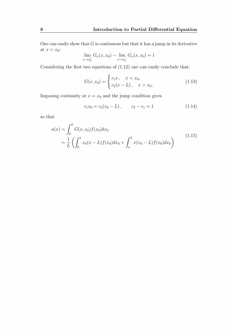
One can easily show that G is continuous but that it has a jump in its derivativeat x = x0:
limx→x+0
Gx(x, x0)− limx→x−0
Gx(x, x0) = 1
Considering the first two equations of (1.12) one can easily conclude that:
G(x, x0) =
c1x , x < x0,
c2(x− L) , x > x0,(1.13)
Imposing continuity at x = x0 and the jump condition gives
c1x0 = c2(x0 − L) , c2 − c1 = 1 (1.14)
so that
u(x) =
∫ L
0
G(x, x0)f(x0)dx0
=1
L
(∫ x
0
x0(x− L)f(x0)dx0 +
∫ L
x
x(x0 − L)f(x0)dx0
) (1.15)
1.2 Linear Dispersive Waves 9
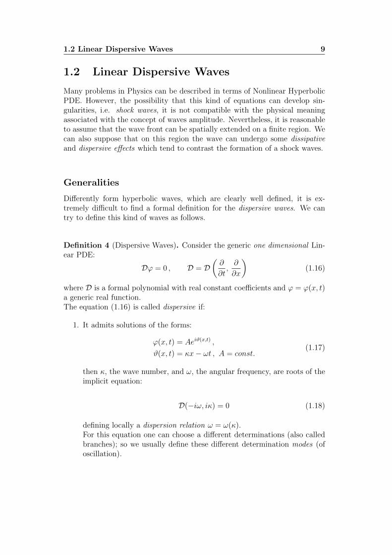
1.2 Linear Dispersive Waves
Many problems in Physics can be described in terms of Nonlinear HyperbolicPDE. However, the possibility that this kind of equations can develop sin-gularities, i.e. shock waves, it is not compatible with the physical meaningassociated with the concept of waves amplitude. Nevertheless, it is reasonableto assume that the wave front can be spatially extended on a finite region. Wecan also suppose that on this region the wave can undergo some dissipativeand dispersive effects which tend to contrast the formation of a shock waves.
Generalities
Differently form hyperbolic waves, which are clearly well defined, it is ex-tremely difficult to find a formal definition for the dispersive waves. We cantry to define this kind of waves as follows.
Definition 4 (Dispersive Waves). Consider the generic one dimensional Lin-ear PDE:
Dϕ = 0 , D = D(∂
∂t,∂
∂x
)(1.16)
where D is a formal polynomial with real constant coefficients and ϕ = ϕ(x, t)a generic real function.The equation (1.16) is called dispersive if:
1. It admits solutions of the forms:
ϕ(x, t) = Aeiϑ(x,t) ,
ϑ(x, t) = κx− ωt , A = const.(1.17)
then κ, the wave number, and ω, the angular frequency, are roots of theimplicit equation:
D(−iω, iκ) = 0 (1.18)
defining locally a dispersion relation ω = ω(κ).For this equation one can choose a different determinations (also calledbranches); so we usually define these different determination modes (ofoscillation).

10 Introduction to Partial Differential Equation
2. The dispersion relation is real valued, which formally means ω(κ) ∈ R,and
ω′′(κ) 6= 0 , almost everywhere (1.19)
The function ω′′(κ) is then called dispersion.
Consider n ∈ Z, for ϑ(x, t) = 2nπ we have that Reϕ is maximum, instead,for ϑ(x, t) = (2n + 1)π then Reϕ is minimum. In both cases, the equationsdescribes linear manifolds in spacetime (straight lines in 1 + 1 dimensions),which evolves with velocity
vp(κ) =ω(κ)
κ, (Phase Velocity) (1.20)
in the direction specified by the wave number.Moreover, we have that:
κ = ϑx , ω = −ϑt
And then one can easily deduce the following statement
κt + ωx = 0 (1.21)
that clearly follows immediately form the Schwarz’s Lemma (concerning themultiple derivation).The latter equation represent the conservation of the number of maxima ofϑ(x, t).
Example 2. Consider the Schrodinger equation
iϕt + γϕxx = 0 , ϕ ∈ C (1.22)
If we propose a solution of this equation of the form:
ϕ(x, t) = A exp [i(κx− ωt)] , A = const.
we obtain that (ω, κ) must undergo the following dispersion relation:
ω − γκ2 = 0
Thus, the Schrodinger equation, if γ ∈ R \ 0, is a dispersive wave equationwith dispersion ω′′(κ) = 2γ.

1.2 Linear Dispersive Waves 11
Wave Packets
From the linearity of the equation (1.16), the general solution of the latter canbe cast as a superposition of monochromatic plane waves
ϕ(x, t) =
∫dκA(κ) exp [i(κx− ω(κ)t)] (1.23)
where A(κ) is an arbitrary function of the wave number. A solution of thisform is called wave packet.As we know from the previous section, the quantity ω′′(κ) is non vanishing,then the phase velocity of any wave composing the wave packet depends onthe wave number κ; vp = vp(κ). Consequently, the wave packet spreads out ast flows.
Although the wave packet tends to spread out with time, the wave packetstill carries information that can be detected for t 1, in an appropriatetime-scale. Given that, in such time the wave packet (more properly, the sin-gle waves composing the packet) will have been propagated also in space then,from the condition t 1, clearly it follows that x 1 in an appropriatespace-scale.Then, it is convenient to study the behaviour of the wave packet in the limitsuch that
t→∞, x→∞, x
t→ O(1)
This case is realized for an observer which, in some way, travels along the wave,as we will clarifier later.Let us therefore study the wave packet in this limit.We can recast the equation (1.23) as follows:
ϕ(x, t) =
∫dκA(κ) exp (−it χ(κ, x/t))
χ(κ, x/t) = −κ xt
+ ω(κ)(1.24)
which clearly shows that, per unit of κ, the exponential oscillate rapidly.Using the saddle point approximation one can prove that, in this limit, we canobtain the following asymptotic behaviour of the wave packet:
ϕ(x, t) ∼ A(x, t) exp [iΘ(x, t)] (1.25)
with
A(x, t) = A0
√2π
|ω′′(κ0)|t , and Θ(x, t) = κ0x− ω(κ0)t (1.26)
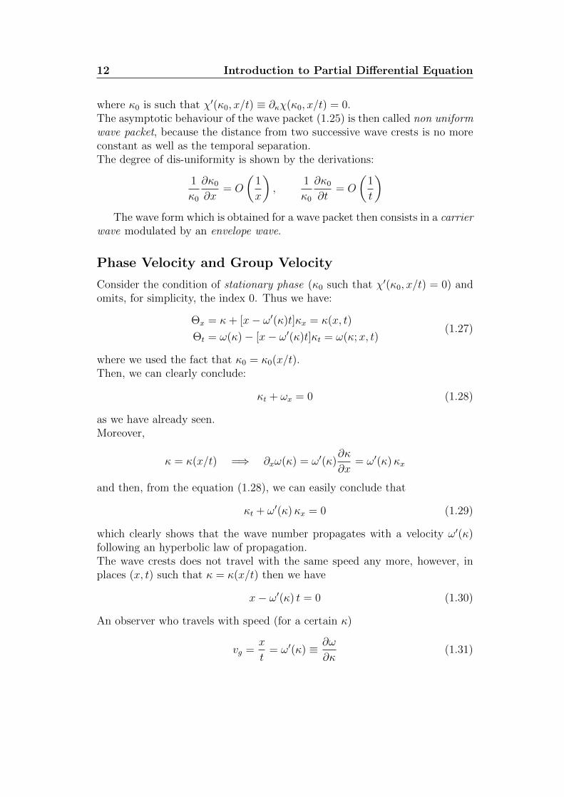
12 Introduction to Partial Differential Equation
where κ0 is such that χ′(κ0, x/t) ≡ ∂κχ(κ0, x/t) = 0.The asymptotic behaviour of the wave packet (1.25) is then called non uniformwave packet, because the distance from two successive wave crests is no moreconstant as well as the temporal separation.The degree of dis-uniformity is shown by the derivations:
1
κ0
∂κ0
∂x= O
(1
x
),
1
κ0
∂κ0
∂t= O
(1
t
)The wave form which is obtained for a wave packet then consists in a carrier
wave modulated by an envelope wave.
Phase Velocity and Group Velocity
Consider the condition of stationary phase (κ0 such that χ′(κ0, x/t) = 0) andomits, for simplicity, the index 0. Thus we have:
Θx = κ+ [x− ω′(κ)t]κx = κ(x, t)
Θt = ω(κ)− [x− ω′(κ)t]κt = ω(κ;x, t)(1.27)
where we used the fact that κ0 = κ0(x/t).Then, we can clearly conclude:
κt + ωx = 0 (1.28)
as we have already seen.Moreover,
κ = κ(x/t) =⇒ ∂xω(κ) = ω′(κ)∂κ
∂x= ω′(κ)κx
and then, from the equation (1.28), we can easily conclude that
κt + ω′(κ)κx = 0 (1.29)
which clearly shows that the wave number propagates with a velocity ω′(κ)following an hyperbolic law of propagation.The wave crests does not travel with the same speed any more, however, inplaces (x, t) such that κ = κ(x/t) then we have
x− ω′(κ) t = 0 (1.30)
An observer who travels with speed (for a certain κ)
vg =x
t= ω′(κ) ≡ ∂ω
∂κ(1.31)
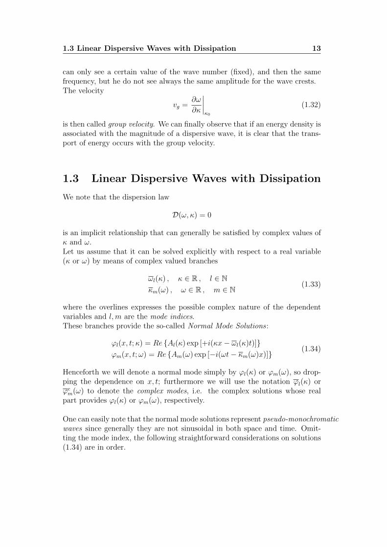
1.3 Linear Dispersive Waves with Dissipation 13
can only see a certain value of the wave number (fixed), and then the samefrequency, but he do not see always the same amplitude for the wave crests.The velocity
vg =∂ω
∂κ
∣∣∣∣κ0
(1.32)
is then called group velocity. We can finally observe that if an energy density isassociated with the magnitude of a dispersive wave, it is clear that the trans-port of energy occurs with the group velocity.
1.3 Linear Dispersive Waves with Dissipation
We note that the dispersion law
D(ω, κ) = 0
is an implicit relationship that can generally be satisfied by complex values ofκ and ω.Let us assume that it can be solved explicitly with respect to a real variable(κ or ω) by means of complex valued branches
ωl(κ) , κ ∈ R , l ∈ Nκm(ω) , ω ∈ R , m ∈ N
(1.33)
where the overlines expresses the possible complex nature of the dependentvariables and l,m are the mode indices.These branches provide the so-called Normal Mode Solutions :
ϕl(x, t;κ) = Re Al(κ) exp [+i(κx− ωl(κ)t)]ϕm(x, t;ω) = Re Am(ω) exp [−i(ωt− κm(ω)x)] (1.34)
Henceforth we will denote a normal mode simply by ϕl(κ) or ϕm(ω), so drop-ping the dependence on x, t; furthermore we will use the notation ϕl(κ) orϕcm(ω) to denote the complex modes, i.e. the complex solutions whose realpart provides ϕl(κ) or ϕm(ω), respectively.
One can easily note that the normal mode solutions represent pseudo-monochromaticwaves since generally they are not sinusoidal in both space and time. Omit-ting the mode index, the following straightforward considerations on solutions(1.34) are in order.

14 Introduction to Partial Differential Equation
1. The first solution of (1.34) is sinusoidal in space with wavelength λ =2π/κ, but it is not necessarily sinusoidal in time, since:
ω(κ) = ωr(κ) + iωi(κ) (1.35)
then, only if ω ∈ R the solution effectively represents a monochromaticwave both in space and time. In general, this wave exhibits a pseudo-period T = 2π/ωr and it propagates with speed (the phase velocity)
vp(κ) :=ωr(κ)
κ(1.36)
exhibiting, if ωi(κ) ≤ 0, an exponential time-decay in amplitude providedby the time-damping factor :
γ(κ) := −ωi(κ) ≥ 0 (1.37)
The last three equations allow us to write a given normal mode as:
ϕ(κ) = exp(−γ(κ)t)Re A(κ) exp [+iκ(x− vp(κ)t)] (1.38)
2. The second solution of (1.34) is sinusoidal in time with period T = 2π/ω,but it is not necessarily sinusoidal in space, since κ may be complex, say
κ(ω) = κr(ω) + iκi(ω) (1.39)
then, only if κ ∈ R the solution effectively represents a monochromaticwave both in space and time. In general, this wave exhibits a pseudo-wavelength λ = 2π/κr and it propagates with speed (the phase velocity)
vp(ω) :=ω
κr(ω)(1.40)
exhibiting, if κi(ω) ≥ 0, an exponential space-decay in amplitude pro-vided by the space-damping factor :
δ(ω) := κi(ω) ≥ 0 (1.41)
The last three equations allow us to write a given normal mode as:
ϕ(ω) = exp(−δ(ω)x)Re A(ω) exp [−iω(t− x/vp(ω))] (1.42)
The (real) solution of a given problem, of type (1) and (2), is assumed to beuniquely determined with complex normal modes by a suitable superposition

1.3 Linear Dispersive Waves with Dissipation 15
of Fourier integrals. Hence, we can write:
ϕ(1)(x, t) =∑l
∫Cl
αl(κ)Al(κ) exp [+i(κx− ωl(κ)t)] dκ =
=∑l
∫Cl
αl(κ)ϕl(κ)dκ
ϕ(2)(x, t) =∑m
∫Cm
βm(ω)Am(ω) exp [−i(ωt− κm(ω)x)] dω =
=∑m
∫Cm
βm(ω)ϕm(ω)dω
(1.43)
where the path of integration C denotes either the real axis R or, when singularpoints occur on it, a suitable parallel line (in the complex plane) which ensurethe convergence and αl(κ), βm(ω) are complex functions to be determined tosatisfy the initial or boundary conditions.
16 Introduction to Partial Differential Equation

Chapter 2
Klein-Gordon Equation withDissipation
Examples of linear hyperbolic systems, which are of physical interest for theirdispersive properties and energy propagation, are provided by the following1-dimensional wave equation.
ϕtt + 2αϕt + β2ϕ = c2ϕxx (2.1)
where ϕ = ϕ(x, t) and α, β, c ∈ R+0 .
In particular, α , β denote two non negative parameters which have dimensionof a frequency [T ]−1 and c denotes the characteristic velocity. When αβ = 0one can recognize some well known equations:
1. D’Alembert Equation when α = β = 0;
2. Klein-Gordon Equation when β > α = 0;
3. Viscoelastic Maxwell Equation when 0 = β < α;
Then, in modern Mathematical Physics, the equation (2.1) is known as theKlein-Gordon Equation with Dissipation (KGD) or Dissipative Klein-GordonEquation.
The KGD is quite interesting since it provides instructive examples both ofnormal dispersion (usually met in the absence of dissipation) and anomalousdispersion (always present in viscoelastic waves). Parameters α and β actuallyplay a fundamental role in the characterization of the dispersion properties ofthe solution and so does the non dimensional parameter m = α/β as well, aswe will see in the next section.
17
18 Klein-Gordon Equation with Dissipation
2.1 Dispersion Relations
The dispersive feature of the KGD are independent from the physical phe-nomenon to which the equation refers since they are obtained formally fromthe associated dispersion relations. Nevertheless, we must distinguish twocases:
(i) Complex frequency ω ∈ C and real wave number κ ∈ R;
(ii) Real frequency ω ∈ R and complex wave number κ ∈ C.
Thus, we agree to write for plane waves:
ϕ(x, t) = A exp(−γt) cos(κx− ωt) , ω = ω − iγϕ(x, t) = A exp(−δx) cos(κx− ωt) , κ = κ+ iδ
(2.2)
where γ > 0 and δ > 0 are usually called time and space attenuation factors,respectively.If we introduce the (2.2) in the KGD we clearly obtain:
−ω2 + c2κ2 − 2iαω + β2 = 0
−ω2 + c2κ2 − 2iαω + β2 = 0(2.3)
which represent the dispersion relations for the KGD.If we consider, for example, the first relation of the (2.3), recalling the definitionω = ω − iγ, we immediately get:
−(ω − iγ)2 + c2κ2 − 2iα(ω − iγ) + β2 = 0 (2.4)
and then
(−ω2 + γ2 + c2κ2 − 2αγ + β2) + i(2ωγ − 2ωα) = 0 (2.5)
thus − ω2 + γ2 + c2κ2 − 2αγ + β2 = 0
2ωγ − 2ωα = 0(2.6)
and we finally obtain the dispersion relation in terms of ω = ω(κ):
ω(κ) = cκ
√1 +
β2 − α2
c2κ2(2.7)
If we now recall the definitions of phase and group velocity, we obtain:
vp(κ) =ω(κ)
κ=
√c2 +
β2 − α2
κ2
vg(κ) =∂ω(κ)
∂κ=
c2κ√c2κ2 + β2 − α2
(2.8)
2.1 Dispersion Relations 19
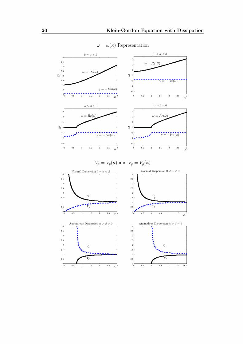
If we quote the plots of the (2.7) and (2.8) we can point out the followingconsideration:
1. For 0 ≤ α < β: vp ≥ vg ≥ 0 - normal dispersion;
2. For 0 ≤ β < α: vg ≥ vp ≥ 0 - anomalous dispersion;
3. For 0 < α = β: vg = vp = c with constant attenuation γ = α andδ = α/c - no dispersion/distortionless.
Now, if we consider the dissipative properties which arise from the KGD wemust again take in account the equations (2.3). If we consider the two cases ofdispersion ((ω, κ) and (ω, κ)), as shown in (2.2), we can immediately concludethat:
ω = ω(κ) = Re(ω)
γ = γ(κ) = −Im(ω)and
κ = κ(ω) = Re(κ)
δ = δ(ω) = Im(κ)(2.9)
Thus, considering the (2.3) we conclude that:
ω = iα±√c2κ2 + (β2 − α2)
|κ(ω)| = 1
c√
2
√(ω2 − β2) +
√(ω2 − β2)2 + (2αω)2
|δ(ω)| = 1
c√
2
√√(ω2 − β2)2 + (2αω)2 − (ω2 − β2)
(2.10)
which gives us an expression for Re(ω), Im(ω), Re(κ) and Im(κ) dependingbasically on κ, ω and sgn(β2 − α2).If we quote the plots of the (2.9) we can point out that in the κ-representationone can notice a cut-off in κ if 0 ≤ β < α, while in the ω-representation thecut-off arise only in absence of dissipation, i.e. α = 0.
20 Klein-Gordon Equation with Dissipation
ω = ω(κ) Representation
0 0.5 1 1.5 2 2.5 30
0.5
1
1.5
2
2.5
3
3.5
40 = α < β
κ
ω
0 0.5 1 1.5 2 2.5 3
−3
−2
−1
0
1
2
3
0 < α < β
κ
ω
0 0.5 1 1.5 2 2.5 3
−3
−2
−1
0
1
2
3
α > β > 0
κ
ω
0 0.5 1 1.5 2 2.5 3
−3
−2
−1
0
1
2
3
α > β = 0
κ
ω
γ = −Im(ω) γ = −Im(ω)
ω = Re(ω)
γ = −Im(ω)
ω = Re(ω)
γ = −Im(ω)
ω = Re(ω) ω = Re(ω)
Vp = Vp(κ) and Vg = Vg(κ)
0 0.5 1 1.5 2 2.5 30
0.5
1
1.5
2
2.5
3
3.5
4Normal Dispersion 0 = α < β
κ 0 0.5 1 1.5 2 2.5 30
0.5
1
1.5
2
2.5
3
3.5
4
Normal Dispersion 0 < α < β
κ
0 0.5 1 1.5 2 2.5 30
0.5
1
1.5
2
2.5
3
3.5
4Anomalous Dispersion α > β > 0
κ 0 0.5 1 1.5 2 2.5 30
0.5
1
1.5
2
2.5
3
3.5
4Anomalous Dispersion α > β = 0
κ
Vp
VgVg
Vg
Vp
VpVp
Vg
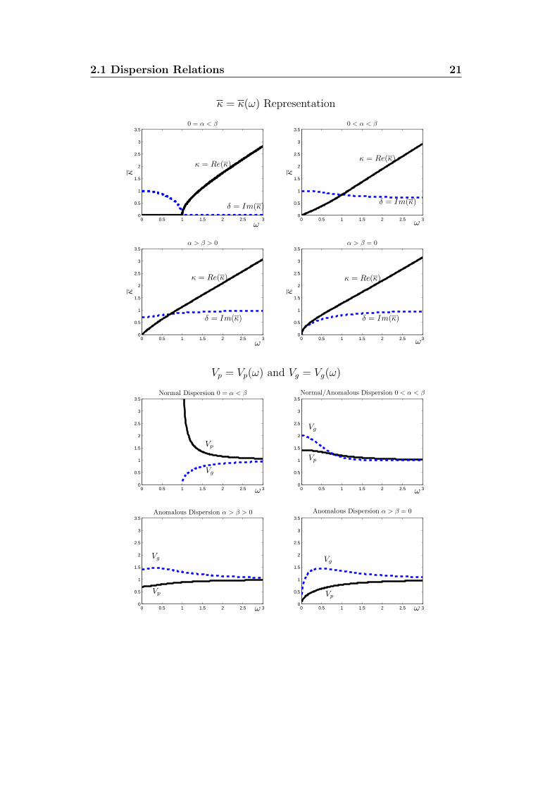
2.1 Dispersion Relations 21
κ = κ(ω) Representation
0 0.5 1 1.5 2 2.5 30
0.5
1
1.5
2
2.5
3
3.5
ω
κ0 = α < β
0 0.5 1 1.5 2 2.5 30
0.5
1
1.5
2
2.5
3
3.50 < α < β
ω
κ
0 0.5 1 1.5 2 2.5 30
0.5
1
1.5
2
2.5
3
3.5α > β > 0
ω
κ
0 0.5 1 1.5 2 2.5 30
0.5
1
1.5
2
2.5
3
3.5α > β = 0
ω
κ
δ = Im(κ)
δ = Im(κ) δ = Im(κ)
κ = Re(κ)κ = Re(κ)
δ = Im(κ)
κ = Re(κ) κ = Re(κ)
Vp = Vp(ω) and Vg = Vg(ω)
0 0.5 1 1.5 2 2.5 30
0.5
1
1.5
2
2.5
3
3.5Normal Dispersion 0 = α < β
ω 0 0.5 1 1.5 2 2.5 30
0.5
1
1.5
2
2.5
3
3.5Normal/Anomalous Dispersion 0 < α < β
ω
0 0.5 1 1.5 2 2.5 30
0.5
1
1.5
2
2.5
3
3.5Anomalous Dispersion α > β > 0
ω 0 0.5 1 1.5 2 2.5 30
0.5
1
1.5
2
2.5
3
3.5
Anomalous Dispersion α > β = 0
ω
Vg
Vg
Vg
Vp
Vp
Vp Vp
Vg
22 Klein-Gordon Equation with Dissipation
2.2 The Signalling Problem
As usual for any PDE occurring in mathematical physics, we must specifysome boundary conditions in order to guarantee the existence, the uniquenessand, in some lucky cases, the determination of a solution of physical interestto the problem.The two basic problems for PDE’s are usually referred to as the Signallingproblem and the Cauchy problem. The former consist in a mixed initial andboundary value problem where the solution is to be found for x > 0 and t > 0,from the data prescribed at t = 0 and x = 0.
Considering the KGD equation (2.1), we propose the following conditions forthe Signalling Problem:
ϕ(x, 0) = ϕt(x, 0) = 0;
ϕ(0, t) = Ψ(t);
ϕ(+∞, t) = 0
for x ≥ 0, t ≥ 0 (2.11)
Then, if we consider the (2.1), the solution of this equation can be easilyobtained using the Laplace transform technique.Indeed, if we recall the definition of the Laplace Transform with respect to thetime variable t:
f(s) ≡ L[f(t)] :=
∫ ∞0
e−stf(t)dt , f(t)÷ f(s) (2.12)
we can clearly conclude that
ϕt(x, t)÷ sϕ(x, s)− ϕ(x, 0) , ϕtt(x, t)÷ s2ϕ(x, s)− sϕ(x, 0)− ϕt(x, 0)
and then, applying these results to the KGD and considering the bound-ary/initial conditions furnished by the Signalling Problem (2.11), one can con-clude that:
ϕtt + 2αϕt + β2ϕ = c2ϕxxL
=⇒ s2ϕ+ 2αsϕ+ β2ϕ = c2ϕxx (2.13)
thus
ϕxx − δ ϕ = 0 , δ =s2 + 2αs+ β2
c2(2.14)
with the boundary/initial conditions:ϕ(0, s) = Ψ(s);
ϕ(+∞, s) = 0(2.15)
2.2 The Signalling Problem 23
The equation (2.14) is an ordinary differential equation in the spatial coordi-nate x which is extremely easy to solve. Indeed, the general solution for the(2.14) is given by:
ϕ(x, s) = c1(s) exp(√δ x) + c2(s) exp(−
√δ x) (2.16)
Now, considering the conditions (2.15) one can easily conclude that:
c1(s) = 0 , c2(s) = Ψ(s)
thus
ϕ(x, s) = Ψ(s) exp(−√δ x) , δ =
s2 + 2αs+ β2
c2(2.17)
or, more explicitly
ϕ(x, s) = Ψ(s) exp(−xc
√(s+ α)2 + β2 − α2
)(2.18)
Now, if we define
τ = t− x
c, ξ =
x
c, χ =
√|β2 − α2| (2.19)
and
F+(ξ, τ) :=J1
(χ√τ(τ + 2ξ)
)√τ(τ + 2ξ)
, if β2 − α2 > 0
F−(ξ, τ) :=I1
(χ√τ(τ + 2ξ)
)√τ(τ + 2ξ)
, if β2 − α2 < 0
(2.20)
then we have:
ϕ(x, s)÷ ϕ(x, t) = Ψ ∗ L−1[exp
(−xc
√(s+ α)2 ± χ2
)]=
= Ψ ∗[e−αξδ(τ)∓ χξe−αξe−ατ F±(ξ, τ) Θ(τ)
] (2.21)
thus
ϕ(ξ, τ) = exp(−αξ)[Ψ(τ)∓ χξ exp(−ατ)F±(ξ, τ) ∗ Ψ(τ)
](2.22)
where J1 and I1, which appear in F±, denote the ordinary and the modifiedBessel function of the first order, respectively.Clearly, the first term of the equation (2.22) represents the input signal, prop-agating at velocity c and exponentially attenuated in space; the second one is
24 Klein-Gordon Equation with Dissipation
responsible for the distortion of the signal that depends on the position and onthe time elapsed from the wave front. The amount of distortion can be mea-sured by the parameter χ that indeed vanishes for α = β, which represents thedistortion-less case.
Remark. The convolution is to be intended in Laplace sense:
(f ∗ g)(t) :=
∫ t
0
f(t− τ)g(τ)dτ
Moreover, Θ(τ) is the Heaviside step function.

2.3 The Cauchy Problem 25
2.3 The Cauchy Problem
Let us now consider the Cauchy problem (or initial value problem), where thesolution is to be found for x ∈ R and t > 0 from the data prescribed at t = 0.Consider the KGD problem; if we rename the function ϕ = ϕ(x, t) as:
ϕ(x, t) = e−αtv(x, t) (2.23)
the equation (2.1) immediately become:
vtt − c2vxx ± χ2v = 0 (2.24)
which clearly is the one dimensional Klein-Gordon equation with m2 = ±χ2.If we want to study the initial value problem for the latter equation then wehave to solve the following Cauchy problem:
vtt − c2vxx ± χ2v = S0δ(x)δ(t)
v(x, 0) = U0δ(x)
vt(x, 0) = V0δ(x)
x ∈ R, t > 0 (2.25)
where v = v(x, t), α, β, c ∈ R+0 and S0, U0, V0 ∈ R (with initial conditions
suitable for a PDE of the second order in time).If we now apply to (2.40) both Laplace (with respect to t) and Fourier Trans-forms (with respect to x) we get:
v(κ, s) =S0 + V0 + U0s
s2 ± χ2 + c2κ2(2.26)
thus we have that the initial condition V0 6= 0 provides a solution similar tothat provided by the source S0 6= 0.Therefore, the problem is divided into three cases.
Case 1 - U0 = V0 = 0In this particular case we have that the equation (2.26) becomes:
v(κ, s) ≡ GS(κ, s) =S0
s2 ± χ2 + c2κ2(2.27)
where GS = GS(x, t) represents the Green’s function for the Source Problem.If we reverse the Fourier Transform we immediately get:
GS(x, s) =S0
2π
∫ +∞
−∞
eiκx
s2 + c2κ2 ± χ2dκ =
S0
π
∫ +∞
0
cos(κx)
s2 + c2κ2 ± χ2dκ (2.28)
26 Klein-Gordon Equation with Dissipation
If we now reverse the Laplace Transform using the following result:
sinαt ÷ α
s2 + α2
we obtain:
GS(x, t) =S0
π
∫ ∞0
cos(κx) sin(t√c2κ2 ± χ2
)√c2κ2 ± χ2
dκ (2.29)
and, recalling the following results:
J0
(α√t2 − A2
)Θ(t− A) ÷ exp
(−A√s2 + α2
)√s2 + α2
I0
(α√t2 − A2
)Θ(t− A) ÷ exp
(−A√s2 − α2
)√s2 − α2
we finally conclude that:
G+S (x, t) =
S0
2cJ0
(χ√t2 − (x/c)2
)Θ(ct− |x|) , if β2 − α2 > 0
G−S (x, t) =S0
2cI0
(χ√t2 − (x/c)2
)Θ(ct− |x|) , if β2 − α2 < 0
(2.30)
Case 2 - S0 = U0 = 0Now we have that the equation (2.26) becomes:
v(κ, s) ≡ G2C(κ, s) =V0
s2 ± χ2 + c2κ2(2.31)
where G2C = GS(x, t) represents the Green’s function for the Second CauchyProblem.As we said before, this case provide a Green’s Function such that
G2C ∝ GS
indeed we can conclude that:
G+2C(x, t) =
V0
2cJ0
(χ√t2 − (x/c)2
)Θ(ct− |x|) , if β2 − α2 > 0
G−2C(x, t) =V0
2cI0
(χ√t2 − (x/c)2
)Θ(ct− |x|) , if β2 − α2 < 0
(2.32)
2.3 The Cauchy Problem 27
Case 3 - S0 = V0 = 0In this case we have:
v(κ, s) ≡ G1C(κ, s) =U0s
s2 ± χ2 + c2κ2=U0s
c2
1s2±χ2
c2+ κ2
(2.33)
If we now reverse the Fourier Transform using the following result:
F−1
[2a
a2 + κ2
]= exp(−a|x|)
then we conclude:
G1C(x, s) =1
2c
U0s√s2 ± χ2
exp
(−|x|c
√s2 ± χ2
)(2.34)
thus,
G1C(x, s) =U0
2cs
exp(− |x|
c
√s2 ± χ2
)√s2 ± χ2
(2.35)
Then, if one consider the following results:
e−Aβδ(t− A) +d
dt
[e−βtI0
(α√t2 − A2
)Θ(t− A)
]÷ s
exp(−A√
(s+ β)2 − α2)
√(s+ β)2 − α2
e−Aβδ(t− A) +d
dt
[e−βtJ0
(α√t2 − A2
)Θ(t− A)
]÷ s
exp(−A√
(s+ β)2 + α2)
√(s+ β)2 + α2
one can immediately conclude that:
G+1C(x, t) =
U0
2c
δ
(t− |x|
c
)+d
dt
[J0
(χ√t2 − (|x|/c)2
)Θ
(t− |x|
c
)]if β2 − α2 > 0
G−1C(x, t) =U0
2c
δ
(t− |x|
c
)+d
dt
[I0
(χ√t2 − (|x|/c)2
)Θ
(t− |x|
c
)]if β2 − α2 < 0
(2.36)
28 Klein-Gordon Equation with Dissipation
Now, if we define:
Λ+(x, t) := J0
(χ√t2 − (|x|/c)2
), if β2 − α2 > 0
Λ−(x, t) := I0
(χ√t2 − (|x|/c)2
), if β2 − α2 < 0
(2.37)
then we can rewrite the Green’s Functions for the equation (2.40) (PDE inv = v(x, t)) as follows:
G±S (x, t) =S0
2cΛ±(x, t)Θ(ct− |x|)
G±1C(x, t) =U0
2c
δ
(t− |x|
c
)+d
dt
[Λ±(x, t)Θ
(t− |x|
c
)]G±2C(x, t) =
V0
2cΛ±(x, t)Θ(ct− |x|)
(2.38)
and then follows the Green’s Functions for the equation (2.1)
G±S (x, t) =S0
2ce−αtΛ±(x, t)Θ(ct− |x|)
G±1C(x, t) =U0
2ce−αt
δ
(t− |x|
c
)+d
dt
[Λ±(x, t)Θ
(t− |x|
c
)]G±2C(x, t) =
V0
2ce−αtΛ±(x, t)Θ(ct− |x|)
(2.39)
Now, if we consider the General Cauchy Problem for the KGD:ϕtt − c2ϕxx + 2αϕt + β2ϕ = 0
ϕ(x, 0) = Φ(x)
ϕt(x, 0) = Ψ(x)
x ∈ R, t > 0 (2.40)
where ϕ = ϕ(x, t) and α, β, c ∈ R+0 ; the solution is clearly is given by:
ϕ(x, t) = G±1C(x, t) ∗ Φ(x) + G±2C(x, t) ∗Ψ(x) (2.41)
fact which conclude this analysis.
Part II
Inflationary Cosmology
29

Chapter 3
The Physics of Inflation
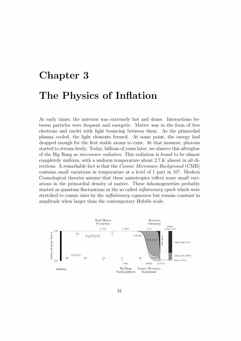
At early times, the universe was extremely hot and dense. Interactions be-tween particles were frequent and energetic. Matter was in the form of freeelectrons and nuclei with light bouncing between them. As the primordialplasma cooled, the light elements formed. At some point, the energy haddropped enough for the first stable atoms to exist. At that moment, photonsstarted to stream freely. Today, billions of years later, we observe this afterglowof the Big Bang as microwave radiation. This radiation is found to be almostcompletely uniform, with a uniform temperature about 2.7K almost in all di-rections. A remarkable fact is that the Cosmic Microwave Background (CMB)contains small variations in temperature at a level of 1 part in 104. ModernCosmological theories assume that these anisotropies reflect some small vari-ations in the primordial density of matter. These inhomogeneities probablystarted as quantum fluctuations in the so called inflationary epoch which werestretched to cosmic sizes by the inflationary expansion but remain constant inamplitude when larger than the contemporary Hubble scale.
31

32 The Physics of Inflation
This picture of the universe is an experimental fact.The majority of the actual universe consists of strange forms of matter andenergy which we have never seen in High Energy Physics experiments. Darkmatter is required to explain the stability of galaxies and the rate of formationof large-scale structures. Dark energy is required to rationalise the strikingfact that the expansion of the universe started to accelerate recently (a fewbillion years ago). Unfortunately, what dark matter and dark energy are isstill unknown.
Another experimental fact is that particle physics processes dominated thevery early eras of the Universe. Quantum field theory effects were predom-inant in this epoch then this leads to an important possibility: scalar fieldsproducing repulsive gravitational effects could have dominated the dynamics ofthe very early universe. This leads to the Theory of the Inflationary Universe,proposed by Alan Guth in 1981.This particular repulsive effect can happen if a scalar field dominates the dy-namics of the early universe and then an extremely short period of acceleratingexpansion will precede the Hot Big Bang era. This produces a very cold andsmooth vacuum-dominated state and ends in ”reheating” which consists in theconversion of the scalar field to radiation, initiating the hot big bang epoch.This inflationary process is claimed to explain the puzzles related to the Causallimitations and the peculiarities of our universe (homogeneity, isotropy, spa-tial curvature). Inflationary expansion explains these features because particlehorizons in inflationary Friedmann-Lemaitre-Robertson-Walker (FLRW) mod-els would be much larger than in the standard models with ordinary matter,allowing causal connection of matter on scales larger than the visual horizon.
3.1 Introduction to Standard Cosmology
Let start to consider the basic theoretical framework which enables to interpretthe cosmological observations. The starting point is the Cosmological Principlewhich states that it is possible to define in space-time a family of space-likesections (space-like foliation of spacetime) such that on top of all of them theUniverse has the same physical properties in each point and in every direction(homogeneity and isotropy).We consider a 4-dimensional Lorentzian manifold (a spacetime) compatiblewith the cosmological principle: the most general metric for such a spacehaving homogeneous and isotropic spatial sections (i.e. which has a maximallysymmetric three-dimensional subspace) can be parametrized by the following
3.1 Introduction to Standard Cosmology 33
line element:
ds2 = −dt2 + a2(t)
[dr2
1− kr2+ r2(dθ2 + sin2 θdφ2)
](3.1)
where a(t) is known as the cosmic scale factor, the parameter k = 1, 0,−1is the curvature constant (corresponding respectively to spherical, euclideanand hyperbolic spatial sections) and (t, r, θ, φ) are known as comoving co-ordinates (they are related to physical coordinates xip by the scale factora(t), i.e. xp = a(t)x). An observer whose 4-velocity in these coordinatesis Uµ = (1, 0, 0, 0) is called a comoving observer and t is the physical timeexperienced by a comoving observer.Another fundamental coordinate choice is obtained by substituting in the pre-vious FRW metric:
dt = a(t(η))dη (3.2)
where η is often called conformal time, whereas t is the cosmic time.
The Einstein Field equations can be derived from the action
S = SEH + Sm. (3.3)
where
SEH =1
2κ2
∫d4x√−g(R− 2Λ) , Einstein-Hilbert Action
Sm =∑fields
∫d4x√−gLfield , ”Matter” Action
(3.4)
and where we included the Cosmological Constant Λ. Then we have the fieldequations:
Gµν + Λgµν = 8πGNTµν with c = 1 (3.5)
where we introduced the Einstein tensor
Gµν := Rµν −1
2Rgµν
and we used the definition
Tµν :=2√−g
δSmδgµν
By using the Bianchi identity ∇νGµν = 0 one can recover the continuity equa-tion for the sources:
∇νTµν = 0 (3.6)
34 The Physics of Inflation
Now, inserting the FRW metric (3.1) into (3.5) we get the so called Friedmannequations :
H2 +k
a2=
8πGN
3ρ+
Λ
3
H +H2 ≡ a
a= −4πGN
3ρ
(1 +
3p
ρ
)+
Λ
3
(3.7)
where p and ρ are respectively the pressure and the energy density of ”matter”and H(t) = a/a is the Hubble Parameter.The cosmological principle fixes the form of the stress-energy tensor to
T µν = a2(t) diag(−ρ, p, p, p)
so the continuity equation for the sources can be rewritten in a non covariantform as
ρ+ 3H(ρ+ p) = 0 (3.8)
where an overdot stands for derivative with respect to the cosmic time t.Among possible sources, we may also include the so-called vacuum or darkenergy, whose equation of state is
ρΛ = −pΛ =Λ
8πGN
(3.9)
The previous relation (3.8) implies that assuming a barotropic equation ofstate for the cosmological fluid, p = wρ we obtain
ρ ∝ a−3(w+1) (3.10)
To keep contact with standard notation we introduce
Ωm :=8πGN
3H2ρ , ΩΛ :=
Λ
3H2, Ωk := − k
(aH)2(3.11)
The critical energy density ρc corresponds to:
ρc :=3H2
0
8πGN
= 8.10h2 × 10−47GeV 4 , h ' (0.71± 0.03) (3.12)
Finally, if we define the deceleration factor q0 as:
q0 := − aaa2
∣∣∣∣t0
(3.13)

3.1 Introduction to Standard Cosmology 35
then we get the two fundamental equations of Standard Cosmology:
Ωm + ΩΛ + Ωk = 1 , q0 =Ωm0
2
(1 +
3p
ρ
)− ΩΛ0 (3.14)
We can solve the equations (3.7), or alternatively any of the equation (3.7)and equation (3.8), to find the qualitative evolution of the cosmic scale factoronce p = p(ρ) is known.Any stable energy component with negative pressure is of little importance inthe early stage of the cosmological evolution: at early times it must have beena minor fraction of the cosmological source because of (3.10).One can immediately derive the evolution of the scale factor for w = 1/3, butthe time coordinate cannot, for this case, be extended beyond a critical valuein the past, conventionally set to t = 0, where a singularity is met almostunavoidably if the dominant energy source has p/ρ > 0.Clearly this analysis is based on Classical General Relativity and breaks downat t ∼ tP
1. The singularity is not a formal artifact of our characteristic solu-tion, but within the framework of General Relativity it has been demonstratedby Hawking and Penrose under well defined, but reasonable, hypotheses.
Theorem 2 (Penrose-Hawking Singularity Theorem). Let M be a globallyhyperbolic space-time with non-compact Cauchy surfaces satisfying the nullenergy condition. If M contains a trapped surface Σ then M is future nullgeodesically incomplete.
Or, more simply: a spacetime M necessarily contains incomplete, inex-tendible timelike or null geodesics (i.e. a singularity) under the followinghypotheses:
1. M contains no closed timelike curves (unavoidable causality require-ment);
2. At each point in M and for each unit timelike vector with componentuα the energy momentum tensor satisfies (null energy condition):(
Tµν −1
2gµνT
αα
)uµuν ≥ 0
3. The manifold is not too highly symmetric so that for at least one pointthe curvature is not lined up with the tangent through the point;
1Planck time: tP =√
~GN
c5 ' 5.39106× 10−44 s
36 The Physics of Inflation
4. M does not contain any trapped surface.
All conditions except the last one, which is rather technical, are completelyreasonable for a realistic spacetime.
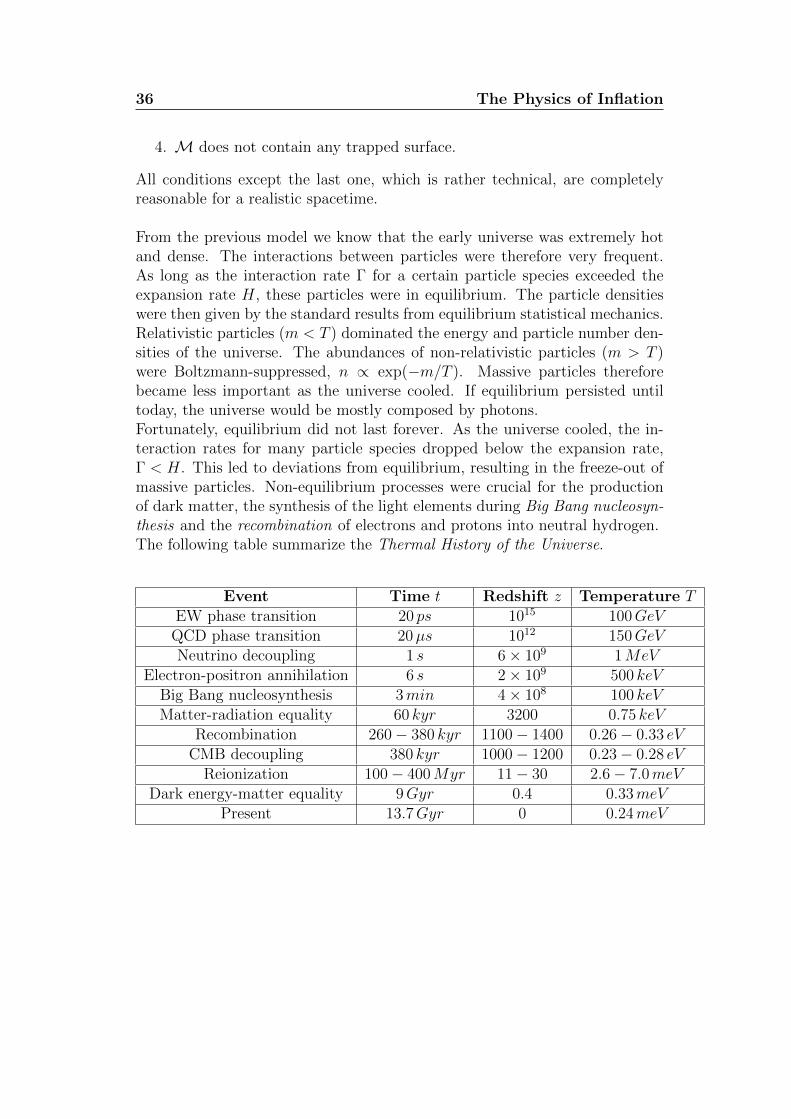
From the previous model we know that the early universe was extremely hotand dense. The interactions between particles were therefore very frequent.As long as the interaction rate Γ for a certain particle species exceeded theexpansion rate H, these particles were in equilibrium. The particle densitieswere then given by the standard results from equilibrium statistical mechanics.Relativistic particles (m < T ) dominated the energy and particle number den-sities of the universe. The abundances of non-relativistic particles (m > T )were Boltzmann-suppressed, n ∝ exp(−m/T ). Massive particles thereforebecame less important as the universe cooled. If equilibrium persisted untiltoday, the universe would be mostly composed by photons.Fortunately, equilibrium did not last forever. As the universe cooled, the in-teraction rates for many particle species dropped below the expansion rate,Γ < H. This led to deviations from equilibrium, resulting in the freeze-out ofmassive particles. Non-equilibrium processes were crucial for the productionof dark matter, the synthesis of the light elements during Big Bang nucleosyn-thesis and the recombination of electrons and protons into neutral hydrogen.The following table summarize the Thermal History of the Universe.
Event Time t Redshift z Temperature TEW phase transition 20 ps 1015 100GeV
QCD phase transition 20µs 1012 150GeVNeutrino decoupling 1 s 6× 10⁹ 1MeV
Electron-positron annihilation 6 s 2× 10⁹ 500 keVBig Bang nucleosynthesis 3min 4× 10⁸ 100 keVMatter-radiation equality 60 kyr 3200 0.75 keV
Recombination 260− 380 kyr 1100− 1400 0.26− 0.33 eVCMB decoupling 380 kyr 1000− 1200 0.23− 0.28 eV
Reionization 100− 400Myr 11− 30 2.6− 7.0meVDark energy-matter equality 9Gyr 0.4 0.33meV
Present 13.7Gyr 0 0.24meV
3.2 Inflation 37
3.2 Inflation
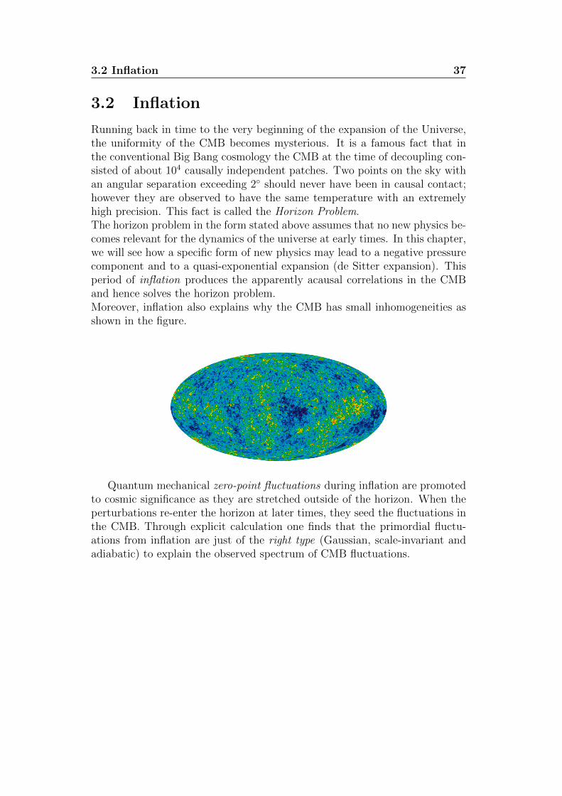
Running back in time to the very beginning of the expansion of the Universe,the uniformity of the CMB becomes mysterious. It is a famous fact that inthe conventional Big Bang cosmology the CMB at the time of decoupling con-sisted of about 104 causally independent patches. Two points on the sky withan angular separation exceeding 2 should never have been in causal contact;however they are observed to have the same temperature with an extremelyhigh precision. This fact is called the Horizon Problem.The horizon problem in the form stated above assumes that no new physics be-comes relevant for the dynamics of the universe at early times. In this chapter,we will see how a specific form of new physics may lead to a negative pressurecomponent and to a quasi-exponential expansion (de Sitter expansion). Thisperiod of inflation produces the apparently acausal correlations in the CMBand hence solves the horizon problem.Moreover, inflation also explains why the CMB has small inhomogeneities asshown in the figure.
Quantum mechanical zero-point fluctuations during inflation are promotedto cosmic significance as they are stretched outside of the horizon. When theperturbations re-enter the horizon at later times, they seed the fluctuations inthe CMB. Through explicit calculation one finds that the primordial fluctu-ations from inflation are just of the right type (Gaussian, scale-invariant andadiabatic) to explain the observed spectrum of CMB fluctuations.
38 The Physics of Inflation
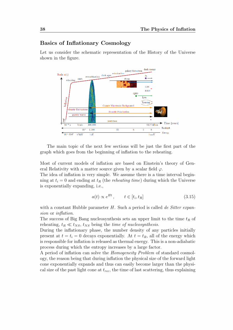
Basics of Inflationary Cosmology
Let us consider the schematic representation of the History of the Universeshown in the figure.
The main topic of the next few sections will be just the first part of thegraph which goes from the beginning of inflation to the reheating.
Most of current models of inflation are based on Einstein’s theory of Gen-eral Relativity with a matter source given by a scalar field ϕ.The idea of inflation is very simple. We assume there is a time interval begin-ning at ti = 0 and ending at tR (the reheating time) during which the Universeis exponentially expanding, i.e.,
a(t) ∝ eHt , t ∈ [ti, tR] (3.15)
with a constant Hubble parameter H. Such a period is called de Sitter expan-sion or inflation.The success of Big Bang nucleosynthesis sets an upper limit to the time tR ofreheating, tR tNS, tNS being the time of nucleosynthesis.During the inflationary phase, the number density of any particles initiallypresent at t = ti = 0 decays exponentially. At t = tR, all of the energy whichis responsible for inflation is released as thermal energy. This is a non-adiabaticprocess during which the entropy increases by a large factor.A period of inflation can solve the Homogeneity Problem of standard cosmol-ogy, the reason being that during inflation the physical size of the forward lightcone exponentially expands and thus can easily become larger than the physi-cal size of the past light cone at trec, the time of last scattering, thus explaining
3.2 Inflation 39
the near isotropy of the cosmic microwave background (CMB). Inflation alsosolves the flatness problem.Most importantly, inflation provides a mechanism which in a causal way gen-erates the primordial perturbations required for galaxies, clusters and evenlarger objects. In inflationary Universe models, the Hubble radius (apparenthorizon) and the (actual) horizon (the forward light cone) do not coincide atlate times. Provided that the duration of inflation is sufficiently long, thenall scales within our present apparent horizon were inside the horizon sinceti. Thus, it is in principle possible to have a causal generation mechanism forperturbations.The density perturbations produced during inflation, as already said, are dueto quantum fluctuations in the matter and gravitational fields. The amplitudeof these inhomogeneities corresponds to a temperature TH ∼ H, the Hawkingtemperature of the de Sitter phase. This leads one to expect that at all timest during inflation, perturbations with a fixed physical wavelength λ ∼ H−1
will be produced. Consequently, the length of the waves is stretched with theexpansion of space, and soon becomes much larger than the Hubble radiuslH(t) = H−1(t). The phases of the inhomogeneities are random. Thus, the in-flationary Universe scenario predicts perturbations on all scales ranging fromthe comoving Hubble radius at the beginning of inflation to the correspondingquantity at the time of reheating. In particular, provided that inflation lastssufficiently long, perturbations on scales of galaxies and beyond will be gener-ated. Note, however, that it is very dangerous to interpret de Sitter Hawkingradiation as thermal radiation. In fact, the equation of state of this ”radiation”is not thermal.
The basic physical mechanism for producing a period of inflation in the veryearly universe relies on the existence, at such epochs, of matter in a form thatcan be described classically in terms of a scalar field. Upon quantisation, ascalar field describes a collection of spin-less particles. It may at first seemrather arbitrary to postulate the presence of such scalar fields in the veryearly universe. However, their existence is suggested by the Standard Modelof Fundamental Interactions, which predict that the Universe experienced asuccession of phase transitions2 in its early stages as it expanded and cooled.For example, let us model this expansion by assuming that the Universe fol-lowed a standard radiation-dominated Friedmann model in its early stages, in
2The basic premise of Grand Unification is that the known symmetries of the elementaryparticles resulted from a larger symmetry group. Whenever a phase transition occurs, partof this symmetry is lost, so the symmetry group changes.

40 The Physics of Inflation
this case:
a(t) ∝√t ∝ 1
T (t)(3.16)
where the ”temperature” T is related to the typical particle energy by T ∼E/kB.The basic scenario is as follows.
• EP ∼ 1019GeV > E > EGUT ∼ 1015GeV The earliest point at whichthe Universe can be modelled as a classical system is the Planck era,corresponding to particle energies EP ∼ 1019GeV and time scales tP ∼10−43 s; prior to this epoch, it is considered that the Universe can bedescribed only in terms of some, as yet unknown, Quantum theory ofGravity.At these extremely high energies, Grand Unified Theories (GUTs) pre-dict that the electroweak and strong forces are unified into a single forceand that these interactions bring the particles present into thermal equi-librium. Once the universe has cooled enough to EGUT ∼ 1014GeV ,there is a spontaneous breaking of the symmetry group characterisingthe GUT into a product of smaller symmetry groups and the electroweakand strong forces separate. From the equation (3.16), this GUT phasetransition occurs at tGUT ∼ 10−36 s.
• EGUT ∼ 1015GeV > E > EEW ∼ 100GeV During this period theelectroweak and strong forces are separate and these interactions sustainthermal equilibrium. This continues until the Universe has cooled toEEW ∼ 100GeV when the unified electroweak theory predicts that asecond phase transition should occur in which the electromagnetic andweak forces separate. Again, the equation (3.16), this electroweak phasetransition occurs at tEW ∼ 10−11 s.
• EEW ∼ 100GeV > E > EQH ∼ 100MeV During this period the elec-tromagnetic, weak and strong forces are separate, as they are today.It is remarkable, however, that when the universe has cooled to EQH ∼100MeV there is a final phase transition, according to the theory ofQuantum Chromodynamics (QCD), in which the strong force increasesin strength and leads to the confinement of quarks into hadrons.This Quark-Hadron phase transition occurs at tQH ∼ 10−5 s.
In general, phase transitions occur via a process called Spontaneous Symme-try Breaking, which can be characterised by the acquisition of certain non-zerovalues by scalar parameters known as Higgs fields. The symmetry is manifestwhen the Higgs fields have the value zero; it is spontaneously broken whenever
3.2 Inflation 41
at least one of the Higgs fields becomes non-zero. Thus, the occurrence ofphase transitions in the very Early Universe suggests the existence of scalarfields and hence provides the motivation for considering their effect on theexpansion of the Universe. In the context of inflation, we will confine our at-tention to scalar fields present at, or before, the GUT phase transition.
For simplicity, let us consider a single scalar field ϕ present in the very EarlyUniverse. The field ϕ is traditionally called the inflaton field for obvious rea-sons.In most current models of inflation, ϕ is a scalar matter field with standardaction:
Lm = −1
2∇µϕ∇µϕ− V (ϕ) , Sm =
∫d4x√−gLm (3.17)
where ∇µ denotes the covariant derivative, g is the determinant of the metrictensor and the exponential expansion is driven by the potential energy densityV (ϕ).The resulting energy-momentum (comparing the result from the variationalapproach with the energy-momentum tensor for a perfect fluid, using comovingcoordinates) tensor yields the following expressions for the energy density ρand the pressure p:
ρ(ϕ) =ϕ2
2+
(∇ϕ)2
2a2+ V (ϕ)
p(ϕ) =ϕ2
2− (∇ϕ)2
6a2− V (ϕ)
(3.18)
It thus follows that if the scalar field is homogeneous and static, but with pos-itive potential energy, then the equation of state p = −ρ, which is necessaryfor exponential inflation, arises.
Most of the current realizations of potential-driven inflation are based on sat-isfying the conditions:
ϕ2 V (ϕ) , a−2(∇ϕ)2 V (ϕ) (3.19)
via the idea of slow rolling.If we now consider the equation of motion of the scalar field ϕ:
ϕ+ 3Hϕ− a−2∆ϕ+dV
dϕ= 0 (3.20)
If the scalar field starts out almost homogeneous and at rest, if the Hubbledamping term is large and if the potential is quite flat, so the term on the
42 The Physics of Inflation
r.h.s. is small, then ϕ may remain small compared to V (ϕ). Note that if thespatial gradient terms are initially negligible, they will remain negligible.
Chaotic inflation is a prototype of inflationary scenario. Consider a scalarfield ϕ which is very weakly coupled to itself and other fields. In this case,ϕ need not to be in thermal equilibrium at the Planck time and most of thephase space for ϕ will correspond to large values of |ϕ| (typically |ϕ| MP ).Consider now a region in space where at the initial time ϕ is very large, approx-imately homogeneous and static. In this case, the energy-momentum tensorwill be immediately dominated by the large potential energy term and inducean equation of state p ' −ρ which leads to inflation. Because of the largeHubble damping term in the scalar field equation of motion, ϕ will only rollvery slowly towards ϕ = 0, assuming that V (ϕ) has a global minimum at afinite value of ϕ which can then be chosen to be ϕ = 0. The kinetic energycontribution to ρ and p will remain small, the spatial gradient contributionwill be exponentially suppressed due to the expansion of the Universe (a(t)increases rapidly) and thus inflation persists. Note that the form of V (ϕ) isirrelevant to the mechanism.It is difficult to realize chaotic inflation in conventional Supergravity Modelssince gravitational corrections to the potential of scalar fields typically renderthe potential steep for values of ϕ of the order of MP and larger.This prevents the slow rolling condition (3.19) from being realizable. Evenif this condition can be satisfied, there are constraints from the amplitude ofproduced density fluctuations which are much harder to satisfy.
Actually, there are many models of potential-driven inflation, but there isno canonical theory. A lot of attention is being devoted to implementing in-flation in the context of Unified Theories, the most important candidate beingSuperstring Theory or M-theory. String Theory or M-theory live in 10 or11 space-time dimensions, respectively. When compactified3 to 4 space-timedimensions, there exist many moduli fields, scalar fields which describe flat di-rections in the complicated vacuum manifold of the theory. A lot of attentionhas recently been devoted to attempts at implementing inflation using modulifields. Not long ago, it has been suggested that our space-time is a Brane in ahigher-dimensional space-time. Ways of obtaining inflation on the Brane arealso under active investigation.It should also not be forgotten that inflation can arise from the purely Gravi-tational sector of the theory, as in the original model of Starobinsky or that it
3In mathematics, compactification is the process or result of making a topological spaceinto a compact space (a space which contains its accumulation points).

3.3 k-Inflation 43
may arise from kinetic terms in an effective action as in pre-big-bang cosmol-ogy or in k-inflation.Theories with (almost) exponential inflation generically predicts an (almost)scale-invariant spectrum of density fluctuations. Via the Sachs-Wolfe effect,these density perturbations induce CMB anisotropies with a spectrum whichis also scale-invariant on large angular scales.The heuristic picture is as follows. If the inflationary period which lasts from tito tR is almost exponential, then the physical effects which are independent ofthe small deviations from exponential expansion are time-translation-invariant.This implies, for example, that quantum fluctuations at all times have the samestrength when measured on the same physical length scale.If the inhomogeneities are small, they can be described by linear theory, whichimplies that all Fourier modes k evolve independently. The exponential expan-sion stretches the wavelength of any perturbation. Thus, the wavelength ofperturbations generated early in the inflationary phase on length scales smallerthan the Hubble radius soon becomes equal to the (existent) Hubble radiusand continues to increase exponentially. After inflation, the Hubble radiusincreases as t while the physical wavelength of a fluctuation increases only asa(t). Thus, eventually the wavelength will cross the Hubble radius again attime tf (k). Thus, it is possible for inflation to generate fluctuations on cosmo-logical scales by causal physics.
3.3 k-Inflation
Much of Modern Cosmology has dealt with the construction of phenomeno-logically suitable inflationary models with various potentials and number ofinflaton fields. In the early stages of inflationary theory there were hopes ofincorporating inflation in more or less standard particle physics. One of thevarious proposals consisted in assuming a close relation between the inflatonfields and the GUTs-transition. However, this idea never worked out in aconvincing way and, consequently, inflation fields lived their own life quite de-tached from the rest of Theoretical Particle Physics.Nowadays, the most important theoretical picture, aiming to unify the mod-ern inflationary cosmology with the theory of fundamental interactions, consistin String Theory. In this theory it is well known that parameters describingbackground geometries and compactifications, the moduli, are all promotedinto scalar fields. There are, therefore, no lack of potential candidates for theinflaton, even though there are several difficult conditions to be met.For one thing, the potential of the inflaton must be extremely flat in order to
44 The Physics of Inflation
allow for enough e-foldings4. On the other hand, it cannot be completely flatfor the idea to work. In Supersymmetric String Theory there are many flatdirections in the moduli space of solutions which could serve as useful startingpoints. The hope would then be that these flat directions are lifted by non-perturbative, supersymmetry breaking terms. Unfortunately, it is difficult tofind these non-perturbative corrections explicitly and their expected form isanyway, in many cases, not of the right kind. In addition, there are also otherproblems to be solved. Apart from the flat, inflationary potential, one needspotentials that manage to fix dangerous moduli like those controlling the size ofthe extra dimensions. It is hard to see how realistic inflationary theories canbe obtained without addressing this problem at the same time.It can be proven that realistic inflationary models can indeed be constructedusing string moduli if one introduces Branes, but this is not the purpose ofthis work. The very basic idea is to use two stacks of Branes separated by acertain distance, corresponding to the inflaton, in a higher dimensional space.As the Branes move, the inflaton rolls, and when the Branes collide inflationstops.Firstly, I will treat the attempts which go under the name of String Cosmol-ogy. The idea is to make use of the dilaton, i.e. the field corresponding to theway the string coupling varies over space and time, and a variant of the stringtheoretical T-duality. The resulting theory fulfils the condition for inflation,albeit in an unorthodox way.On second instance, it will be presented a very recent theoretical tool of in-flationary cosmology theory, known as k-inflation, aiming to help to locatewhich sector of string theory has inflated a strongly curved initial state intoour presently observed large and weakly curved Universe.
3.3.1 Basics of String Cosmology
String cosmology makes use of one of the most basic features of string theory,the concept of dilaton. According to string theory the Einstein-Hilbert actionof General Relativity is described by a new dimensionless scalar field, thedilaton ϕ, and given by
S = − 1
2κ210
∫d10x√−g e−ϕ (R + ∂αϕ∂αϕ) (3.21)
where κ10 = (2π)7α′4/2 ∼ l8s and where the string coupling is related to thedilaton through g2
s = eϕ. The action as given is written in the string frame.
4E-folding is the time interval in which an exponentially growing quantity increases by afactor of e.

3.3 k-Inflation 45
That is, the string length, ls, is our fundamental unit and what we use as ourmeasuring rod. This means that the Planck mass, the effective coefficient ofthe scalar curvature R, varies with the dilaton. An alternative way to describethings is to use the Einstein frame which in many ways is physically more clearthan the string frame. In the Einstein frame it is the Planck length, which ismore directly related to macroscopic physics through the strength of gravity,which is used as a fundamental unit. Let me explain the relation between thetwo frames in more detail.Immediately, one can note that that the frames are, by definition, relatedthrough∫
dDx√−ge−ϕR =
∫dDx√−gE(RE + · · · ) , gµν = e2ωϕ(gE)µν (3.22)
where the subscript E indicate the Einstein frame and furthermore
√−g = eDωϕ√−gE (3.23)
It follows, from the definition of curvature, that the scalar curvatures arerelated through
R = e−2ωϕ[RE − 2ω(D − 1)∆ϕ− ω2(D − 2)(D − 1)∂αϕ∂αϕ
](3.24)
Hence we have that
√−ge−ϕR =√−gEe(Dω−1−2ω)ϕ
[RE − 2ω(D − 1)∆ϕ− ω2(D − 2)(D − 1)∂αϕ∂αϕ
]and consequently
Dω − 1− 2ω = 0 =⇒ ω =1
D − 2(3.25)
The action in the Einstein frame finally becomes
S = −MD−2D
2
∫dDx√−gE
(RE −
1
D − 2∂αϕ∂αϕ
)(3.26)
also called the D-dimensional Einstein-Hilbert Action, where MD is the D-dimensional Planck mass. We note that the sign of the kinetic term of thescalar field now is the familiar one.If we consider a metric of FRW-form (3.1) generalized to D dimensions, wefind
ds2E = e−2ωϕds2 = e−2ωϕ
(−dt2 + a2(t)dx2
)≡ −dt2E + a2
E(t)dx2 (3.27)
46 The Physics of Inflation
whereaE(t) := e−ωϕa(t) , dtE := e−ωϕdt (3.28)
It is important to realize that the two frames are physically equivalent, even ifthings can, at a first glance, look rather different in the two frames. To fullyappreciate string cosmology it is important to keep this in mind.
Let us now investigate the above action in more detail. I will perform theanalysis in the string frame, and, for simplicity, assume a spatially homoge-nous FRW-metric. One can readily check that the scalar curvature in thesecoordinates is given by
R = −(D − 1)(D − 2)a
a− 2(D − 1)
a
a(3.29)
The action possesses a remarkable symmetry thanks to the presence of thestringy dilaton. The symmetry acts on the scale factor and the dilaton throughthe transformations
a(t) −→ 1/a(t)
ϕ(t) −→ ϕ(t)− 2(D − 1) ln a(t)(3.30)
It leaves the action invariant and assures that the solutions of the equationsof motion have some very interesting properties that will be important forcosmology. To verify the symmetry, we note that
√−ge−ϕ(R+ϕ2) = aD+1e−ϕ
[−(D − 1)
(a
a
)2
+
(ϕ− (D − 1)
a
a
)2]
+Total Derivative
(3.31)Since we have (considering the equations (3.30))
aD−1e−ϕ −→ aD−1e−ϕ
a
a−→ − a
a
(3.32)
we find
aD+1e−ϕ
[−(D − 1)
(a
a
)2
+
(ϕ− (D − 1)
a
a
)2]−→
−→ aD+1e−ϕ
[−(D − 1)
(a
a
)2
+
(ϕ− (D − 1)
a
a
)2] (3.33)
and hence an invariance of the action.In other words, if a(t) and ϕ(t) solves the equations of motion, so does the
3.3 k-Inflation 47
transformed functions 1/a(t) and ϕ(t)− 2(D − 1) ln a(t).To fully appreciate what is going on, and to understand the structure of thesolutions, we need to note that there is yet another simple symmetry
t −→ −t (3.34)
i.e. time reversal invariance, which together with (3.30) presents an interestingfact about possible cosmologies.
Combining the two symmetries we can map out how various solutions arerelated to each other. If we first consider the scale factor a(t), we can eas-ily see how we can construct two new solutions, from a given solution a(t),according to
a(t) −→ 1/a(t) , H(t) −→ −H(t)
a(t) −→ a(−t) , H(t) −→ −H(−t) (3.35)
The time t = 0 is referred to as the Big Bang and it is natural to allow for twoeras, a pre and a post Big Bang. The basic idea of String Cosmology is thatphysics can be traced back in time through the Big Bang into an earlier era,the pre Big Bang, where many of the initial conditions for the post Big Bangare determined in a natural and dynamical way.
It should be remarked that the whole previous formulation is in line withthe general picture of T-duality in String Theory. According to T-duality, itis equivalent to compactify string theory on a small circle (compared with thestring scale) and a large circle.In some sense large and small scales are, therefore, equivalent. Loosely apply-ing this idea to the Big Bang, would suggest that if we trace the expansion farenough back in time, we are better off describing the universe as becoming big-ger again, rather than smaller. As can be proven, however, string cosmologysuggests that we should take an expanding pre Big Bang theory and match itto an expanding post Big Bang. But this is the picture obtained in the stringframe. The picture in the Einstein frame is quite different with a contractingrather than an expanding pre Big Bang phase. This is precisely in line withthe hand waving argument above.

48 The Physics of Inflation
3.3.2 A brief introduction to k-Inflation
The inflationary paradigm offers the attractive possibility of resolving manyof the puzzles of standard hot big bang cosmology. The crucial ingredient ofmost successful inflationary scenarios is a period of ”slow-roll” evolution of theinflaton field, ϕ, during which the potential energy density V (ϕ) , stored in ϕ,dominates its kinetic energy ϕ2/2 and drives a quasi-exponential expansion ofthe Universe.As previously mentioned, String Theory provides one with several very weaklycoupled scalar fields, the moduli, which could be natural inflaton candidates,however, their non-perturbative potentials V (ϕ) do not seem to be able tosustain a slow-roll inflation because, for large values of ϕ, they tend either togrow, or to tend to zero, too fast. It is therefore important to explore novelpossibilities for implementing an inflationary evolution of the early Universe.The main feature of the so known Kinetically Driven Inflation (k-inflation)consist in the fact that, even in absence of any potential energy term, a gen-eral class of non-standard (non-quadratic) kinetic energy terms, for a scalarfield ϕ, can drive an inflationary evolution of the same type as the usually con-sidered potential driven inflation. By ”usual type of inflation” we mean herean accelerated expansion (in the Einstein conformal frame η) during which thecurvature scale starts around a Planckian value and then decreases monoton-ically.By contrast, the pre big bang scenario uses a standard quadratic kinetic en-ergy term ϕ2/2 to drive an accelerated contraction (in the Einstein frame)during which the curvature scale increases. Though we shall motivate belowthe consideration of non-standard kinetic terms by appealing to the existence,in string theory, of higher-order corrections to the effective action for ϕ. Withthese statements we do not claim that the structure needed for implementingour kinetically driven inflation arises inevitably in string theory but we payattention to a new mechanism for implementing inflation.
Let me introduce the basic formalism of the k-Inflation.As we have already mentioned, slow-roll ination assumes that the kinetic termis canonical, Ls.r. = X − V (ϕ) where X ≡ −1
2∂µϕ∂µϕ.
As one can easily see, a given FRW background with time-dependent Hubbleparameter H(t) corresponds to cosmic acceleration if and only if:
ε := − H
H2< 1 (3.36)
For this condition to be sustained for a sufficiently long time, requires
|ζ| := |ε|Hε 1 (3.37)
3.3 k-Inflation 49
i.e. the fractional change of ε per Hubble time is small.Now, considering the slow-roll approximation (3.19) we than obtain:
ε = − H
H2≈ M2
P
2
(V ′
V
)2
=: εv
|ζ| = |ε|Hε≈M2
P
|V ′′|V
=: |ζv|(3.38)
where εv and ζv are the so called potential slow-roll parameters.One can immediately understand that when these are small, slow-roll inflationoccurs, thus:
εv =M2
P
2
(V ′
V
)2
1 , |ζv| = M2P
|V ′′|V 1 (3.39)
Now, if one consider that the kinetic term of the slow roll Lagrangian Densityis canonical, this puts strong constraints on the shape of the potential V (ϕ)via the potential slow-roll conditions. However, these conditions for inflationare not absolute, but assume the slow-roll approximations.In contrast, the Hubble slow-roll conditions, ε, ζ 1 do not make any approx-imations and allow for a larger spectrum of inflationary backgrounds. In par-ticular, the constraints on the inflationary potential can potentially be relaxedif higher-derivative corrections to the kinetic term were dynamically relevantduring inflation, i.e. |H| H2 not because the theory of potential-dominated,but because it allows non-trivial dynamics.A useful way to describe these effects is by the following action,
S =
∫d4x√−g
[M2
PR
2+ P (X,ϕ)
](3.40)
with
P (X,ϕ) =∑n
cn(ϕ)Xn
Λ4n−4(3.41)
For X Λ4, the dynamics reduces to that of slow-roll inflation, so we are nowinterested in the limit X ∼ Λ4. This is an extremely complicated situationbecause X/Λ4 controls the derivative expansion. In particular, in the limitX → Λ4 we have to worry about the appearance of unstable ”ghost” statesand the stability under radiative corrections. Specifically, in the absence ofsymmetries, there is no way to protect the coefficients cn in (3.41) from quan-tum corrections. The predictions derived from (3.41) then cannot be trusted.However, sometimes the theory is equipped with a symmetry that forbids largerenormalizations of these coefficients.
50 The Physics of Inflation
This is the case, for instance in Dirac-Born-Infeld (DBI) inflation, wherea higher-dimensional boost symmetry protects the special form of the La-grangian Density
P (X,ϕ) = −Λ4(ϕ)
√1 +
X
Λ4(ϕ)− V (ϕ) (3.42)
In this case, the boost symmetry forces quantum corrections to involve the two-derivative combination. We remark that, only when they come with protectivesymmetries are P (X)-theories really interesting and predictive theories.The stress-energy tensor arising from (3.40) has pressure P and energy density
ρ = 2XP,X − P (3.43)
where P,X denotes a derivative with respect to X. The inflationary parameterε then becomes:
ε = − H
H2=
3XP,X2XP,X − P
(3.44)
The condition for inflation is still ε 1, which now is a condition on thefunctional form of P (X). However, it should be remembered that unless aprotective symmetry is identified, there is no guarantee that the P (X)-theoryis radiatively stable.The fluctuations in P (X)-theories have a number of interesting features. First,in the limit X ∼ Λ4, they propagate with a non-trivial speed of sound
c2s =
dP
dρ=
P,XP,X + 2XP,XX
(3.45)
The limit of small sound speed implies enhanced interactions in the cubic andquartic Lagrangian. This leads to large amount of non-Gaussian perturbations.

Chapter 4
Tachyon Matter Cosmology
Let us begin with the question: What are Tachyons? Historically, these weredescribed as particles which travel faster than light. If we use the relativisticequation:
v =pc√
p2 +m2c2(4.1)
relating the velocity v of a particle to its momentum p, mass m and the veloc-ity of light c, then we see that tachyons can also be regarded as particles withnegative mass squared (or, equivalently, with an imaginary mass).Of course, both descriptions sound equally bizarre. On the other hand tachyonshave been known to exist in String Theory almost since its birth and hence weneed to make sense of them.
Actually, tachyons do appear in conventional Quantum Field Theories (QFT)as well. Consider, for instance, a classical scalar field ϕ with potential V (ϕ).For simplicity I shall set ~ = c = 1. Consider a (p + 1)-space, labelled by thetime coordinate x0 and space coordinates xi, with 1 ≤ i ≤ p; then the theLagrangian Density of the scalar field is:
L = −1
2∂µϕ∂µϕ− V (ϕ) ≡ 1
2
(∂0ϕ∂0ϕ− ∂iϕ∂iϕ
)− V (ϕ) (4.2)
Normally, we choose the origin of ϕ so that the potential V (ϕ) has a minimumat ϕ = 0. In this case, the quantization of ϕ gives a scalar particle such that:
m2ϕ =
d2V
dϕ2(0) > 0 (4.3)
which gives a real mass mϕ. Nevertheless, if we suppose that the potential hasa maximum at ϕ = 0, then we conclude that:
m2ϕ =
d2V
dϕ2(0) < 0 (4.4)
51
52 Tachyon Matter Cosmology
thus, the quantization of ϕ gives a tachyon.In this case, however, we can easily conclude that this way of thinking is com-pletely wrong. When we identify V ′′(0) = m2
ϕ we are making an approximation.We expanded V (ϕ) in a Taylor series expansion in ϕ and treated the cubic andhigher order terms as small corrections to the quadratic term. This is actuallytrue only if the quantum fluctuations of ϕ around ϕ = 0 are small. Hence, wedo not have tachyons in QFT of a scalar field.Thus we see that the existence of a tachyon in a scalar field theory impliesthat the potential for the scalar field has a local maximum at the origin. Inorder for the theory to be sensible at least in perturbation theory, the poten-tial must also have a (local) minimum. Typically, whenever the potential in ascalar field theory has more than one extremum we can construct non-trivialclassical solutions which depend on one or more spatial directions, but this isnot the aim of this work.The lessons learned from the field theory may be summarized as follows:
1. Existence of tachyons in the spectrum tells us that we are expanding thepotential around its maximum rather than its minimum;
2. The correct procedure to deal with such a situation is to find the (global)minimum of the potential and expand the potential around the minimum.The resulting theory has a positive mass2 scalar particle instead of atachyon;
3. Associated with the existence of tachyons we often have non-trivial spacedependent classical solutions.
We now turn to the discussion of Tachyons in String Theory. The con-ventional description of string theory is based on ”first quantized” formalismrather than a field theory. We take a string (closed or open) and quantize itmaintaining Lorentz invariance. This gives infinite number of states character-ized by momentum p and other discrete quantum numbers n. It turns out thatthe energy of the n-th state carrying momentum p is given by En =
√p2 +m2
n,where mn is some constant. This state clearly has the interpretation of beinga particle of mass mn. Thus string theory contains infinite number of single”particle” states, as if it were a field theory with infinite number of fields.Quantization of some closed or open strings gives rise to states with negativem2n for some n. This clearly corresponds to a tachyon. For instance, the orig-
inal bosonic string theory, formulated in 25 + 1 dimensions, has a tachyon inthe spectrum of closed strings. This theory is thought to be inconsistent dueto this reason.Superstring Theories are free from tachyons in the spectrum of closed string,
4.1 Introduction 53
but, for certain boundary conditions, there can be tachyon in the spectrumof open strings even in Superstring Theories. Thus the question is: Does theexistence of tachyons make the theory inconsistent? Or does it simply indicatethat we are quantizing the theory around the wrong point?The problem in studying this question stems from the fact that unlike theexample in a scalar field theory, the tachyon in string theory does not origi-nally come from quantization of a scalar field. Hence, in order to understandthe tachyon, we have to reconstruct the scalar field and its potential from theknown results in string theory, and then analyse if the potential has a mini-mum.It turns out that for open string tachyons we now know the answer in manycases. On the other hand, closed string tachyons are only beginning to beexplored.
4.1 Introduction
There are many faces of Superstring/Brane Cosmology which come from dif-ferent sectors of M/String Theories. In particular, many people search forpotential candidates to explain Early Universe Inflation. One of the StringTheory constructions, Tachyon on D-branes, has been recently proposed forcosmological applications by A. Sen. A relatively simple formulation of theunstable D-brane tachyon dynamics in terms of Effective Field Theory stimu-lates one to investigate its role in Cosmology.The rolling tachyon in the string theory may be described in terms of EffectiveField Theory for the Tachyon Condensate ϕ, which in the flat spacetime hasa Lagrangian Density:
L = −V (ϕ)√
1− 2X , X ≡ −1
2∂µϕ∂µϕ (4.5)
The tachyon potential V (ϕ) has a positive maximum at ϕ = 0 and a minimumat ϕ0, with V (ϕ0) = 0.It is noteworthy that the models of type (4.5) already were studied in Cos-mology on the phenomenological ground. For certain choices of potentials Vand non-minimal kinetic terms one can get kinematically driven inflation, k-inflation. However, it remains to be seen how this kind of potentials can bemotivated by the String Theory of Tachyon.In this thesis, we investigate cosmology with tachyon matter with a string the-ory motivated potential of the form V ∼ eϕ/ϕ0 . In the next section, we writedown the equations for the tachyon matter coupled to gravity. We focus on
54 Tachyon Matter Cosmology
self-consistent formulation of the isotropic Friedmann- Robertson-Walker cos-mology supported by the tachyon matter. It is described by coupled equationsfor the time-dependent background tachyon field ϕ(t) and the scale factor ofthe universe a(t). Finally, we will study in details small fluctuations of thetachyon field δϕ(x, t) for the previous potential coupled with a suitable infla-ton field.
4.2 Cosmology with Rolling Tachyon Matter
Rolling tachyon is associated with unstable D-branes and self-consistent inclu-sion of gravity may require higher-dimensional Einstein equations with Branes.Still, in the low energy limit, one expects that the Brane Gravity is reducedto the four dimensional Einstein theory.In this section, we consider tachyon matter coupled with Einstein gravity infour dimensions. Then, the model is given by the action:
S =
∫d4x√−g
(R
16πGN
− V (ϕ)√
1 +∇µϕ∇µϕ
)(4.6)
from which follows the Einstein equations and then the field equation for thetachyon:
∇µ∇µϕ− ∇µ∇νϕ
1 +∇αϕ∇αϕ∇µϕ∇νϕ− V,ϕ
V= 0 (4.7)
If we apply these equations for the isotropic, homogeneous and spatially flatFRW cosmological model, then one can conclude that the energy-momentumtensor of tachyon matter is reduced to a diagonal form T µν = diag(−ρ, p, p, p)where the energy density ρ is given by:
ρ =V (ϕ)√1− ϕ2
(4.8)
the pressure p isp = −V (ϕ)
√1− ϕ2 (4.9)
and the equation for the evolution of the scale factor follows from
H2(t) ≡(a
a
)2
=8πGN
3
V (ϕ)√1− ϕ2
(4.10)
The equation for the time-dependent rolling tachyon in an expanding universefollows from (4.7),
ϕ
1− ϕ2+ 3Hϕ+
V,ϕV
= 0 (4.11)

4.3 Fluctuations in Rolling Tachyon 55
4.3 Fluctuations in Rolling Tachyon
The issue of stability of small scalar fluctuations is often essential in scalarfield cosmology. In this very short section, we provide a formalism for treatinglinear inhomogeneous fluctuations in the tachyon field. Let us consider smallinhomogeneous perturbation of the tachyon field δϕ(x, t) around time-dependent background solution ϕ(t) of equation (4.11)
ϕ(x, t) = ϕ(t) + δϕ(x, t) (4.12)
Now, linearizing the field equation (4.7) with respect to small fluctuations δϕwe obtain evolution equation for the time-dependent for the inhomogeneousperturbation δϕ(x, t) in a homogeneous background (ϕ(t)):
δϕ
1− ϕ2+
2ϕϕ
(1− ϕ2)2˙δϕ+ [−∆ + (log V ),ϕϕ] δϕ = 0 (4.13)
that, using the results of the previous section, con be rewritten as follows:
δϕ−(1−ϕ2) ∆δϕ+
[3H(1− 3ϕ2)− 2ϕ
V,ϕV
]˙δϕ+
[V,ϕϕV−(V,ϕV
)2]
(1−ϕ2)δϕ = 0
(4.14)

56 Tachyon Matter Cosmology
4.4 A Toy Model for Inhomogeneous Fluctu-
ations in the Tachyon Cosmology
Let us consider a very simple Toy Model for Inhomogeneous Fluctuations inthe Tachyon Cosmology.As we have already seen in the previous section, linearizing the field equation(4.7) with respect to small fluctuations δϕ we obtain the following evolutionequation for the time-dependent for the inhomogeneous perturbation δϕ(x, t)in a homogeneous background (ϕ(t)):
δϕ−(1−ϕ2) ∆δϕ+
[3H(1− 3ϕ2)− 2ϕ
V,ϕV
]˙δϕ+
[V,ϕϕV−(V,ϕV
)2]
(1−ϕ2)δϕ = 0
(4.15)To analyse the very important case of a tachyon potential which has ϕ0 →∞we use exponential asymptotic of the potential
V (ϕ) ∼ exp(−ϕ/ϕ0) (4.16)
which is derived from the string theory calculations.Dimensional parameters of the potential are related to the fundamental lengthscale, ϕ ∼ ls, and V0 is the Brane Tension. As it was demonstrated by Sen,the tachyon matter is pressure-less for the potential with the ground state atinfinity. In this case, tachyon matter may be considered as an interesting can-didate to represent Cold Dark Matter.Now, if we consider a special case where the Inflaton Field assumes the follow-ing form (homogeneous background):
ϕ(t) ∼√
1− c2 t , c ∈ R (4.17)
then, from (4.16), (4.17) and supposing H(t) ' const., we obtain a simplerevolution equation for the time-dependent for the inhomogeneous perturbationδϕ(x, t):
δϕ− c2∆δϕ+
[3H(3c2 − 2) +
2√
1− c2
ϕ0
]˙δϕ = 0 (4.18)
Just to understand the general behaviour for this kind of inhomogeneous fluc-tuations in Tachyon Cosmology, let us consider the (1+1)-dimensional problemfor the latter equation:
(δϕ)tt − c2(δϕ)xx +
[3H(3c2 − 2) +
2√
1− c2
ϕ0
](δϕ)t = 0 (4.19)
4.4 A Toy Model for Inhomogeneous Fluctuations in the TachyonCosmology 57
which is exactly the Klein-Gordon equation with Dissipation with
2α = 3H(3c2 − 2) +2√
1− c2
ϕ0
, and β2 = 0 (4.20)
If we consider a simple initial condition as
δϕ(x, 0) = 0 , and (δϕ)t(x, 0) = δ(x) (4.21)
from the results of the second chapter, one can immediately conclude that:
δϕ(x, t) = G−2C(x, t) =exp(−αt)
2cI0
(χ√t2 − (x/c)2
)Θ(ct− |x|) (4.22)
where:
α =3
2H(3c2 − 2) +
√1− c2
ϕ0
, χ =√|β2 − α2| = |α| (4.23)
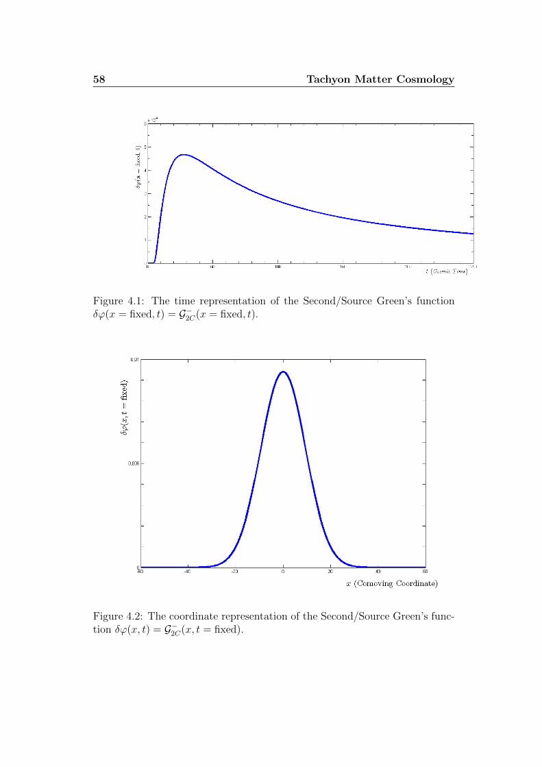
58 Tachyon Matter Cosmology
Figure 4.1: The time representation of the Second/Source Green’s functionδϕ(x = fixed, t) = G−2C(x = fixed, t).
Figure 4.2: The coordinate representation of the Second/Source Green’s func-tion δϕ(x, t) = G−2C(x, t = fixed).
Appendix A
Dispersion Relations -Calculations
Consider the dispersion relation for the KGD:
−ω2 + c2κ2 − 2iαω + β2 = 0
−ω2 + c2κ2 − 2iαω + β2 = 0(A.1)
• Case 1: ω = ω − iγ.From the first equation of (A.1) we get:
−(ω − iγ)2 + c2κ2 − 2iα(ω − iγ) + β2 = 0 (A.2)
and then
(−ω2 + γ2 + c2κ2 − 2αγ + β2) + i(2ωγ − 2ωα) = 0 (A.3)
thus − ω2 + γ2 + c2κ2 − 2αγ + β2 = 0
2ωγ − 2ωα = 0(A.4)
and we finally obtain:
ω = iα±√c2κ2 + (β2 − α2) (A.5)
thus ω(κ) = Re(ω) = ±Re(√
c2κ2 + (β2 − α2))
γ(κ) = −Im(ω) = −α∓ Im(√
c2κ2 + (β2 − α2)) (A.6)
59
60 Dispersion Relations - Calculations
• Case 2: κ = ω + iδ.From the second equation of (A.1) we get:
κ2 =ω2 − β2
c2+ i
2αω
c2(A.7)
Now, if we consider the equation:
z2 = A2 + iB2 , z = x+ iy, x, y ∈ R (A.8)
than we have:
x2 − y2 + 2ixy = A+ iB ⇒A = x2 − y2
B = 2xy(A.9)
thus x2 = y2 + A
y =B
2x
⇔
x2 = y2 + A
y2 =B2
4x2
and then it immediately follows that:
4x4 − 4Ax2 −B2 = 0 (A.10)
If we now define a new variable t = x2 we then obtain:
4t2 − 4At−B2 = 0 (A.11)
thus
x2 = t± =A±√A2 +B2
2(A.12)
Clearly, we can only accept t+ and then we obtain:
x = ± 1√2
√A+√A2 +B2 (A.13)
Now,
y2 = x2 − A =A+√A2 +B2
2− A =
√A2 +B2 − A
2(A.14)
thus: x = ± 1√
2
√A+√A2 +B2
y = ± 1√2
√√A2 +B2 − A
(A.15)
61
This result can immediately lead us to the following conclusion: if were-define κ = x, δ = y, A = (ω2 − β2)/c2 and 2αω/c2 in the equation(A.7), then we obtain the following results:
|κ(ω)| = 1
c√
2
√(ω2 − β2) +
√(ω2 − β2)2 + (2αω)2
|δ(ω)| = 1
c√
2
√√(ω2 − β2)2 + (2αω)2 − (ω2 − β2)
(A.16)
fact which conclude our discussion.

62 Dispersion Relations - Calculations

Bibliography
[1] Sandro Salsa - Equazioni a derivate parziali - Metodi, modelli e appli-cazioni - Springer-Verlag Italia; 2010
[2] A.S. Demidov - Generalized functions in Mathematical Physics - 2001.
[3] P. T. Chrusciel, G. J. Galloway, D. Pollack - Mathematical General Rela-tivity - http://arxiv.org/pdf/1004.1016.pdf .
[4] Daniel Baumann - Cosmology - Part III Mathematical Tripos, DAMTPCambridge (UK).
[5] Francesco Mainardi - Fractional Calculus and Waves in Linear Viscoelas-ticity - Imperial College Press; 2010.
[6] Francesco Mainardi - Signal velocity for transient waves in linear dissipa-tive media - Wave Motion , vol. 5, no. 1, pp. 33− 41; 1983.
[7] Dean G. Duffy - Green’s functions with applications - Chapman & Hall;2001.
[8] J. N. Islam - An Introduction to Mathematical Cosmology - CambridgeUniversity Press; 2004.
[9] C. Armendariz-Picon, T. Damour, V. Mukhanov - k-Inflation -http://arxiv.org/pdf/hep-th/9904075v1.pdf .
[10] Maurizio Gasperini - Theory of Gravitational Interactions - Springer-Verlag Italia; 2013.
[11] Johanna Erdmenger - String Cosmology - Wiley-VCH; 2009.
[12] Maurizio Gasperini - Elements of String Cosmology - Cambridge Univer-sity Press; 2007.
[13] Robert H. Brandenberger - Inflation and the Theory of Cosmological Per-turbations - http://arxiv.org/pdf/astro-ph/9711106.pdf .
63
64 BIBLIOGRAPHY
[14] Robert H. Brandenberger - Frontiers of Inflationary Cosmology -http://arxiv.org/pdf/hep-ph/0102183v1.pdf .
[15] D. Baumann and H. V. Peirisy - Cosmological Inflation: Theory and Ob-servations - http://arxiv.org/pdf/0810.3022v2.pdf .
[16] J. Garriga and V.F. Mukhanov - Perturbations in k-inflation -http://arxiv.org/pdf/hep-th/9904176v1.pdf .
[17] Alan Guth - Inflation - Carnegie Observatories Astrophysics Series, Vol.2: Measuring and Modeling the Universe - Cambridge: Cambridge Univ.Press; 2004.
[18] V. F. Mukhanov - Physical Foundations of Cosmology - Cambridge Uni-versity Press; 2005.
[19] A. Frolov, L. Kofman and A. Starobinsky - Prospects and Problems ofTachyon Matter Cosmology - CITA-2002-09, hep-th/0204187.
[20] D. Bailint and A. Love - Kaluza-Klein theories - Rep. Prog. Phys. 50(1987) 1087-1170.
[21] Steven Weinberg - Cosmology - Oxford University Press; 2008.