dissertation - core.ac.uk
TRANSCRIPT

DISSERTATION
Titel der Dissertation
The Quality-Aware Service Selection Problem:
An Adaptive Evolutionary Approach
Application to the Selection of Distributed Data and Software
Services in the ATLAS Experiment
Verfasserin
Mag. Elisabeth Vinek
angestrebter akademischer Grad
Doktorin der technischen Wissenschaften
(Dr. techn.)
Wien, 2011
Studienkennzahl lt. Studienblatt: A 786 175
Dissertationsgebiet lt. Studienblatt: Wirtschaftsinformatik
Betreuer: Univ.-Prof. Dipl.-Ing. Dr. Erich Schikuta

I dedicate this thesis to my father, in loving and thankful memory.

Abstract
Quality of Service (QoS) is an important aspect in distributed, service-oriented systems. When
several concrete services exist that implement the same functionality, the choice of a service instance
among many can be made based on QoS considerations, objectives and constraints. Typically
considered properties are performance, availability, and costs. When several services need to be
composed in order to respond to a request, the resulting problem is more complex, as local QoS
attributes have to be aggregated into global QoS values for the overall workflow, which is often
spawned across organizational boundaries. To perform this aggregation, the specific attributes as
well as the involved workflow patterns have to be known. Aiming for an optimal service selection can
contribute to significantly reduce overall execution times, costs, or any other specifically formulated
objective. The resulting challenge is referred to as the QoS-aware service selection problem.
In this thesis, aspects of the service selection problem are studied in the context of a distributed,
service-oriented system from ATLAS, a high-energy physics experiment at CERN, the European
Organization for Nuclear Research. In this so-called TAG system, data and modular services are
distributed world-wide and need to be selected and composed on the fly, as a user starts a request.
There are two conflicting optimization viewpoints, one of the user who wants requests to be executed
as fast as possible, and one of the system managers seeking to load-balance between all available
resources, thus optimizing the system throughput. The service selection is modeled as a dynamic
multi-constrained optimal path problem, which allows considering both QoS attributes of service
instances and of the network. The dynamic aspects of the system, such as removed or added
resources, changing attributes and changing optimization objectives are included in the problem
definition, as they represent a specific challenge.
To address these issues regarding dynamics and conflicting viewpoints, this work proposes a
service selection optimization framework based on a multi-objective genetic algorithm capable of
efficiently dealing with changing conditions by using a persistent memory of good solutions, and a
stepwise adaptation of the mutation rate. A system and QoS attribute ontology as well as a descrip-
tion of dynamics of distributed systems build the basis of the framework. The presented approach
is evaluated in terms of optimization quality (approximation of the Pareto front), adaptability to
changes, runtime performance and scalability. Several parts of the overall optimization framework
are ultimately integrated into the TAG system and evaluated therein. Although motivated by a
concrete application, the framework is generally applicable to service selection challenges with spe-
cific characteristics close to the ones of the TAG system. A discussion about the operational effort
of developing and maintaining such an optimization framework is provided and presents a guideline
for the integration in further applications.
i

ii

Kurzfassung
Die Qualitat der Serviceerbringung (kurz QoS fur “Quality of Service”) ist ein wichtiger Aspekt in
verteilten, Service-orientierten Systemen. Wenn mehrere Implementierungen einer Funktionalitat
koexistieren, kann die Wahl eines konkreten Services aufgrund von QoS-Aspekten getroffen werden.
Leistung, Verfugbarkeit und Kosten sind Beispiele fur QoS-Attribute eines Services. Wenn mehrere
Services benotigt werden, um einen Workflow zu bilden, mussen lokale QoS-Attribute zu globalen
Workflow-Attributen aggregiert werden, wobei der resultierende Workflow Services von verschiede-
nen Organisationen umfassen kann. Fur eine solche Aggregation mussen sowohl die Attribute als
auch die Workflowstrukturen bekannt und dokumentiert sein. Eine optimale Selektion von verteil-
ten Services ist erstrebenswert, um zum Beispiel die gesamte Ausfuhrungsdauer, entstehende Kosten
oder sonstige definierte Ziele zu optimieren. Das resultierende Problem wird “QoS-aware Service
Selection Problem” genannt.
In der vorliegenden Dissertation werden Aspekte dieses Selektionsproblems anhand eines kon-
kreten, Service-orientieren Systems vertieft. Es handelt sich dabei um das TAG-System in ATLAS,
einem Hochenergiephysikexperiment am CERN, der Europaischen Organisation fur Kernforschung.
Die Daten und Services des TAG-Systems sind weltweit verteilt und mussen auf Anfrage selektiert
und zu einem Workflow zusammengesetzt werden. Die Optimierung wird aus zwei unterschiedlichen
Blickwinkeln durchgefuhrt: dem eines Benutzers, der seine Anfrage so schnell wie moglich beant-
wortet haben mochte, und dem der Systemmanager, deren Ziel es ist, die Last auf alle zur Verfugung
stehenden Ressourcen zu verteilen und somit den Durchsatz des Systems zu optimieren. Die Se-
lektion wird als ein dynamisches Pfadoptimierungsproblem unter Nebenbedingungen modelliert,
wodurch QoS-Attribute sowohl der Knoten (Services) als auch der Kanten (Netzwerk) berucksichtigt
werden konnen. Die dynamischen Aspekte (z.B. wechselnde Ressourcen, Attribute, Optimierungs-
funktionen oder Gewichte) sind in der Problemformulierung integriert, da sie eine spezifische Her-
ausforderung und Anforderung an Losungsalgorithmen stellen.
Fur die dynamische Pareto-Optimierung von Serviceselektionsproblemen wird im Rahmen dieser
Arbeit ein Optimierungsansatz mit einem genetischen Algorithmus prasentiert, der uber einen persis-
tenten Speicher von fruheren Losungen sowie eine automatische Adaptierung der Mutationsrate eine
effiziente Anpassung an das sich standig verandernde System gewahrleistet. Eine Ontologie der Sys-
temkomponenten sowie deren QoS-Attribute bildet die Basis fur die Optimierung. Der Ansatz wird
im Rahmen der Dissertation hinsichtlich der Qualitat der erzielten Losungen, der Adaptierung an
Anderungen sowie der Laufzeit evaluiert. Teile des Ansatzes wurden schließlich in das TAG-System
integriert und darin evaluiert. Obwohl der Ansatz im Rahmen eines spezifischen Serviceselektion-
sproblems entwickelt wurde, ist er in anderen Szenarien oder Systemen mit ahnlichen Charakeristika
iii

iv
einsetzbar. Die Herausforderungen wahrend der Entwicklung und des Betriebes des Optimierungs-
frameworks werden beschrieben und bilden somit eine Anleitung fur dessen mogliche Integration in
andere Systeme.

Acknowledgements
First and foremost, I would like to thank my adviser, Prof. Erich Schikuta. He has provided me
with excellent guidance through my studies, carefully showing the way to a successful completion as
a balance of curiosity, enthusiasm, and pragmatism. I also particularly thank David Malon from the
Argonne National Laboratory for accepting to review my thesis, and for providing such a motivating
work environment in the ATLAS TAG group.
This thesis work has been carried out at CERN, and I would like to thank Richard Hawkings
for welcoming me in his section, introducing me to the subject and always taking the time to meet
and discuss, while being very busy with first physics at the LHC. I would like to address special
thanks to my office mate Florbela Viegas for discussing with me all aspects of my work, and letting
me profit from her immense knowledge and experience in many areas of computer science. Thanks
also to Gancho Dimitrov, who has been a great office mate during the past three years. It has been
an amazing experience to work in an international team of researchers and engineers – I thank the
members of the ATLAS TAG team for the friendly and encouraging atmosphere.
I am particularly thankful to Peter Paul Beran for numerous fruitful discussions and for being
such a great co-author. Our cross-motivation in the last year has been crucial for completion.
Further, I would like to thank Armin Nairz for his very detailed proof-reading and in general for the
great “TAG - Tier-0” cooperation.
I am grateful to my friends here in Geneva, Austria and elsewhere, for their (remote) support
and the great moments we shared, even if we had little time together in the past three years.
Friedrich, thank you for your encouragement and patience, and for “keeping me in balance,” by
opening my eyes (and ears!) to exciting new things, and enriching my life in so many ways.
Finally, I would like to thank my mother for being a constant support in all matters and encour-
aging me whenever I have doubts.
This work has been supported by the Austrian “Bundesministerium fur Wissenschaft und Forschung”.
v

vi

Contents
Abstract i
Kurzfassung iii
Acknowledgements v
List of Figures xii
List of Tables xiii
List of Algorithms xv
1 Introduction 1
1.1 The QoS-Aware Service Selection Problem . . . . . . . . . . . . . . . . . . . . . . . . 2
1.2 Motivation for a Dynamic and Adaptive Service Selection Optimization Framework . 4
1.3 Challenges and Contributions . . . . . . . . . . . . . . . . . . . . . . . . . . . . . . . 6
1.4 Thesis Structure . . . . . . . . . . . . . . . . . . . . . . . . . . . . . . . . . . . . . . 8
2 Motivation and Application Scenario: TAG-based Metadata Queries in the ATLAS
Experiment 13
2.1 The ATLAS Experiment at the LHC . . . . . . . . . . . . . . . . . . . . . . . . . . . 14
2.2 From RAW Data to Event-Level Metadata: TAGs . . . . . . . . . . . . . . . . . . . 15
2.3 TAG Data and Services . . . . . . . . . . . . . . . . . . . . . . . . . . . . . . . . . . 17
2.3.1 TAG Content . . . . . . . . . . . . . . . . . . . . . . . . . . . . . . . . . . . . 17
2.3.2 TAG Use Cases . . . . . . . . . . . . . . . . . . . . . . . . . . . . . . . . . . . 17
2.3.3 TAG Databases . . . . . . . . . . . . . . . . . . . . . . . . . . . . . . . . . . . 19
2.3.4 TAG Services . . . . . . . . . . . . . . . . . . . . . . . . . . . . . . . . . . . . 20
2.4 Typical TAG Workflows . . . . . . . . . . . . . . . . . . . . . . . . . . . . . . . . . . 21
2.5 Distribution of Data and Services and Resulting Challenge . . . . . . . . . . . . . . . 22
3 Background and Related Work: Service Selection in Heterogeneous Environ-
ments 27
3.1 Basic Concepts . . . . . . . . . . . . . . . . . . . . . . . . . . . . . . . . . . . . . . . 28
3.2 Overview and Comparison of Related Research Areas . . . . . . . . . . . . . . . . . 29
vii

viii CONTENTS
3.3 Modeling Service-Oriented Systems . . . . . . . . . . . . . . . . . . . . . . . . . . . . 32
3.3.1 System Models . . . . . . . . . . . . . . . . . . . . . . . . . . . . . . . . . . . 32
3.3.2 QoS Attributes . . . . . . . . . . . . . . . . . . . . . . . . . . . . . . . . . . . 33
3.3.3 Motivation for an Ontology for QoS-Aware Service Selection . . . . . . . . . 35
3.4 Approaches to solve the QoS-Aware Service Selection Problem . . . . . . . . . . . . 37
3.4.1 Linear Mixed Integer Programming . . . . . . . . . . . . . . . . . . . . . . . . 37
3.4.2 Graph-based Approaches . . . . . . . . . . . . . . . . . . . . . . . . . . . . . 40
3.4.3 Network Topology Approaches . . . . . . . . . . . . . . . . . . . . . . . . . . 41
3.4.4 Game Theory and Bidding . . . . . . . . . . . . . . . . . . . . . . . . . . . . 42
3.4.5 Evolutionary Approaches . . . . . . . . . . . . . . . . . . . . . . . . . . . . . 43
3.4.6 Swarm Intelligence Approaches . . . . . . . . . . . . . . . . . . . . . . . . . . 44
3.4.7 Artificial Neural Networks . . . . . . . . . . . . . . . . . . . . . . . . . . . . . 45
3.5 Multi-Objective Service Selection Optimization . . . . . . . . . . . . . . . . . . . . . 47
4 An Ontology of Components and Attributes of Distributed, Service-Oriented
Systems 49
4.1 Methodology . . . . . . . . . . . . . . . . . . . . . . . . . . . . . . . . . . . . . . . . 50
4.2 System Ontology . . . . . . . . . . . . . . . . . . . . . . . . . . . . . . . . . . . . . . 52
4.2.1 Generic System Ontology . . . . . . . . . . . . . . . . . . . . . . . . . . . . . 52
4.2.2 Application: TAG System Components . . . . . . . . . . . . . . . . . . . . . 54
4.3 Attribute Ontology . . . . . . . . . . . . . . . . . . . . . . . . . . . . . . . . . . . . . 59
4.3.1 Generic Attribute Ontology . . . . . . . . . . . . . . . . . . . . . . . . . . . . 59
4.3.2 Application: TAG System Attributes . . . . . . . . . . . . . . . . . . . . . . . 62
4.3.3 Attribute Aggregation . . . . . . . . . . . . . . . . . . . . . . . . . . . . . . . 67
4.4 TASK - TAG Application Service Knowledge Base . . . . . . . . . . . . . . . . . . . 69
4.4.1 TASK Schema and Services . . . . . . . . . . . . . . . . . . . . . . . . . . . . 69
4.4.2 Gathering System Statistics . . . . . . . . . . . . . . . . . . . . . . . . . . . . 72
4.4.3 Performance and Usage Indexes . . . . . . . . . . . . . . . . . . . . . . . . . . 75
4.5 Summary . . . . . . . . . . . . . . . . . . . . . . . . . . . . . . . . . . . . . . . . . . 76
5 QoS-Aware Service Selection: A Dynamic Multi-Objective Optimization Prob-
lem 77
5.1 Dynamic Aspects of Service-Oriented Systems . . . . . . . . . . . . . . . . . . . . . . 78
5.2 Detecting and Assessing Changes in the Environment . . . . . . . . . . . . . . . . . 82
5.2.1 System Monitoring and Profiles . . . . . . . . . . . . . . . . . . . . . . . . . . 82
5.2.2 Optimization Profiles . . . . . . . . . . . . . . . . . . . . . . . . . . . . . . . 84
5.2.3 Quantifying System Changes . . . . . . . . . . . . . . . . . . . . . . . . . . . 85
5.3 Concrete Problem Formulation . . . . . . . . . . . . . . . . . . . . . . . . . . . . . . 86
5.3.1 Mathematical Model . . . . . . . . . . . . . . . . . . . . . . . . . . . . . . . . 87
5.3.2 Optimization Objectives and Profiles . . . . . . . . . . . . . . . . . . . . . . . 89
5.3.3 Discussion . . . . . . . . . . . . . . . . . . . . . . . . . . . . . . . . . . . . . . 91
5.4 Multi-Objective Optimization in Dynamic Environments . . . . . . . . . . . . . . . . 92
5.4.1 General Problem Statement . . . . . . . . . . . . . . . . . . . . . . . . . . . . 92

CONTENTS ix
5.4.2 Pareto-Optimal Solutions . . . . . . . . . . . . . . . . . . . . . . . . . . . . . 93
5.4.3 Classical Solving Methods . . . . . . . . . . . . . . . . . . . . . . . . . . . . . 94
5.4.4 Dealing with Dynamic Environments . . . . . . . . . . . . . . . . . . . . . . . 96
5.5 Analysis of the Multi-Objective Optimization Problem in the TAG System . . . . . 98
5.6 Summary . . . . . . . . . . . . . . . . . . . . . . . . . . . . . . . . . . . . . . . . . . 99
6 Designing Genetic Algorithms for Service Selection Optimization Problems 103
6.1 Background on Genetic Algorithms . . . . . . . . . . . . . . . . . . . . . . . . . . . . 104
6.1.1 Basic Concepts . . . . . . . . . . . . . . . . . . . . . . . . . . . . . . . . . . . 104
6.1.2 Genetic Algorithms for Multi-Objective Optimization . . . . . . . . . . . . . 106
6.2 Dynamic Genetic Algorithms . . . . . . . . . . . . . . . . . . . . . . . . . . . . . . . 109
6.2.1 Algorithm Restart or Re-Initialization . . . . . . . . . . . . . . . . . . . . . . 110
6.2.2 Diversity after Changes: Adapting the Mutation Rate . . . . . . . . . . . . . 111
6.2.3 Diversity along the Runtime: Modifying the Selection . . . . . . . . . . . . . 111
6.2.4 Memory-based Techniques . . . . . . . . . . . . . . . . . . . . . . . . . . . . . 111
6.2.5 Multi-Population Techniques . . . . . . . . . . . . . . . . . . . . . . . . . . . 112
6.2.6 Comparison . . . . . . . . . . . . . . . . . . . . . . . . . . . . . . . . . . . . . 112
6.3 Motivation for Using GAs in QoS-Aware Service Selection . . . . . . . . . . . . . . . 112
6.4 An Adaptive and Dynamic Multi-Objective Genetic Algorithm for QoS-aware Service
Selection Problems . . . . . . . . . . . . . . . . . . . . . . . . . . . . . . . . . . . . . 114
6.4.1 Problem Encoding . . . . . . . . . . . . . . . . . . . . . . . . . . . . . . . . . 114
6.4.2 Fitness Functions . . . . . . . . . . . . . . . . . . . . . . . . . . . . . . . . . . 114
6.4.3 Genetic Operators and Multi-Objective Design Considerations . . . . . . . . 116
6.4.4 Adaptability to Changes . . . . . . . . . . . . . . . . . . . . . . . . . . . . . . 118
6.4.5 Integrated Optimization Approach with AD-MOGA . . . . . . . . . . . . . . 120
6.4.6 Tuning Possibilities . . . . . . . . . . . . . . . . . . . . . . . . . . . . . . . . . 121
6.5 Related Work . . . . . . . . . . . . . . . . . . . . . . . . . . . . . . . . . . . . . . . . 124
6.6 Summary . . . . . . . . . . . . . . . . . . . . . . . . . . . . . . . . . . . . . . . . . . 128
7 Implementation and Evaluation 131
7.1 Simulation and Evaluation Setup . . . . . . . . . . . . . . . . . . . . . . . . . . . . . 132
7.2 Evaluation Scenario I: Applicability of AD-MOGA, Pareto Approximation and Input
Parameters . . . . . . . . . . . . . . . . . . . . . . . . . . . . . . . . . . . . . . . . . 133
7.3 Evaluation Scenario II: Adaptability to Changes . . . . . . . . . . . . . . . . . . . . 137
7.3.1 Formal Evaluation Criteria for Dynamic GA . . . . . . . . . . . . . . . . . . 137
7.3.2 Implementation of the Persistent Memory . . . . . . . . . . . . . . . . . . . . 137
7.3.3 Changes During or Between Optimization Runs . . . . . . . . . . . . . . . . . 138
7.3.4 Stepwise Adaptation of the Mutation Rate . . . . . . . . . . . . . . . . . . . 143
7.4 Evaluation Scenario III: Runtime Performance and Scalability . . . . . . . . . . . . . 145
7.5 Application to the TAG System . . . . . . . . . . . . . . . . . . . . . . . . . . . . . . 148
7.6 Practical Considerations for the Implementation . . . . . . . . . . . . . . . . . . . . 152
7.7 Possible Extensions in Future Work . . . . . . . . . . . . . . . . . . . . . . . . . . . 154
7.8 Summary . . . . . . . . . . . . . . . . . . . . . . . . . . . . . . . . . . . . . . . . . . 155

x CONTENTS
8 Conclusion 159
A System and Attribute Ontology: OWL Schemas 161
A.1 OWL Definitions Used in the Ontologies . . . . . . . . . . . . . . . . . . . . . . . . . 161
A.2 System Ontology: OWL Schema . . . . . . . . . . . . . . . . . . . . . . . . . . . . . 162
Glossary 171
Bibliography 183
Curriculum Vitae 185

List of Figures
1.1 Mapping of Abstract to Concrete Workflow . . . . . . . . . . . . . . . . . . . . . . . 3
1.2 Multi-Dimension Multi-Choice Knapsack Problem . . . . . . . . . . . . . . . . . . . 4
1.3 Challenges Addressed in the Thesis . . . . . . . . . . . . . . . . . . . . . . . . . . . . 7
2.1 Computer-generated view of the ATLAS Detector . . . . . . . . . . . . . . . . . . . 14
2.2 LHC Tier-0 and Tier-1 Sites and Network Overview . . . . . . . . . . . . . . . . . . 16
2.3 Data Reconstruction Chain . . . . . . . . . . . . . . . . . . . . . . . . . . . . . . . . 18
2.4 iELSSI Screenshots . . . . . . . . . . . . . . . . . . . . . . . . . . . . . . . . . . . . . 22
2.5 Typical TAG Workflows . . . . . . . . . . . . . . . . . . . . . . . . . . . . . . . . . . 23
2.6 Distributed TAG System . . . . . . . . . . . . . . . . . . . . . . . . . . . . . . . . . . 24
2.7 Execution Times for Query Involving TAG Database and iELSSI . . . . . . . . . . . 25
3.1 Selected Elements of the CIM Core Model . . . . . . . . . . . . . . . . . . . . . . . . 33
3.2 Selected Elements of the CIM Metrics Model . . . . . . . . . . . . . . . . . . . . . . 34
3.3 Classification of Non-Functional Properties . . . . . . . . . . . . . . . . . . . . . . . 36
3.4 Overview of Optimization Approaches for Service Selection Problems . . . . . . . . . 37
3.5 Total Enumeration Tree for Branch-and-Bound Algorithms . . . . . . . . . . . . . . 39
3.6 Service Candidate Graph (General Flow Structure) . . . . . . . . . . . . . . . . . . . 41
3.7 ANN Components and Simplified Mathematical Model . . . . . . . . . . . . . . . . . 46
4.1 Areas for Ontology Uses . . . . . . . . . . . . . . . . . . . . . . . . . . . . . . . . . . 51
4.2 Methodology Applied for Building the Ontologies . . . . . . . . . . . . . . . . . . . . 52
4.3 Generic System Ontology: Inferred Class Hierarchy . . . . . . . . . . . . . . . . . . . 54
4.4 Generic System Ontology: OntoGraf Representation . . . . . . . . . . . . . . . . . . 57
4.5 TAG System Model (UML Class Diagram) . . . . . . . . . . . . . . . . . . . . . . . 58
4.6 Subclasses of NonFunctionalAttribute . . . . . . . . . . . . . . . . . . . . . . . . . 63
4.7 Attribute (and System) Ontology: Classes Overview . . . . . . . . . . . . . . . . . . 64
4.8 Workflow Patterns for Composition . . . . . . . . . . . . . . . . . . . . . . . . . . . . 68
4.9 TASK Architecture Overview . . . . . . . . . . . . . . . . . . . . . . . . . . . . . . . 72
4.10 TASK: Data Catalog . . . . . . . . . . . . . . . . . . . . . . . . . . . . . . . . . . . . 73
4.11 TASK: Service Catalog . . . . . . . . . . . . . . . . . . . . . . . . . . . . . . . . . . . 74
5.1 Similarity Index and Change Impact . . . . . . . . . . . . . . . . . . . . . . . . . . . 86
xi

xii LIST OF FIGURES
5.2 Abstract and Concrete Workflow Mapping . . . . . . . . . . . . . . . . . . . . . . . . 89
5.3 Multi-Objective Optimization Problem: Decision and Objective Space . . . . . . . . 93
5.4 Dynamic Online Optimization . . . . . . . . . . . . . . . . . . . . . . . . . . . . . . . 98
5.5 Abstract and Concrete Workflows in a Simple Example . . . . . . . . . . . . . . . . 101
5.6 Pareto Optimal Points for the Simple Example . . . . . . . . . . . . . . . . . . . . . 101
5.7 Pareto Optimal Points for the Simple Example with Changed Attributes . . . . . . . 102
6.1 Genetic Algorithm: Cycle of Operations . . . . . . . . . . . . . . . . . . . . . . . . . 106
6.2 Steps of a Genetic Algorithm . . . . . . . . . . . . . . . . . . . . . . . . . . . . . . . 108
6.3 Chromosome Encoding . . . . . . . . . . . . . . . . . . . . . . . . . . . . . . . . . . . 115
6.4 Schema of the Persistent Memory of Solutions . . . . . . . . . . . . . . . . . . . . . . 120
6.5 Overview of the Optimization Process . . . . . . . . . . . . . . . . . . . . . . . . . . 122
7.1 Simulation Setup: Database Schema . . . . . . . . . . . . . . . . . . . . . . . . . . . 132
7.2 Classes and Packages in the Prototype Implementation . . . . . . . . . . . . . . . . . 133
7.3 Approximation of the Pareto Front: Even Deployment Distribution . . . . . . . . . . 135
7.4 Approximation of the Pareto Front: Uneven Deployment Distribution . . . . . . . . 136
7.5 Schematic Query of the Persistent Memory . . . . . . . . . . . . . . . . . . . . . . . 138
7.6 Changes Between Optimization Runs . . . . . . . . . . . . . . . . . . . . . . . . . . . 140
7.7 10% Change Rate Between Optimization Runs . . . . . . . . . . . . . . . . . . . . . 141
7.8 50% Change Rate Between Optimization Runs . . . . . . . . . . . . . . . . . . . . . 142
7.9 Impact of Adding Deployments with Different Change Rates . . . . . . . . . . . . . 144
7.10 Impact of Varying Mutation Rates, Similarity Index 0.9 . . . . . . . . . . . . . . . . 145
7.11 Impact of Varying Mutation Rates, Similarity Index 0.8 . . . . . . . . . . . . . . . . 146
7.12 Impact of Varying Mutation Rates, Similarity Index 0.7 . . . . . . . . . . . . . . . . 146
7.13 Runtime for Increasing System Setups . . . . . . . . . . . . . . . . . . . . . . . . . . 149
7.14 Composition of the Runtime . . . . . . . . . . . . . . . . . . . . . . . . . . . . . . . . 150
7.15 Integration of the Optimization Approach into the TAG System . . . . . . . . . . . . 151
7.16 Outline of Design and Implementation Steps . . . . . . . . . . . . . . . . . . . . . . . 153
7.17 Areas for Future Extensions . . . . . . . . . . . . . . . . . . . . . . . . . . . . . . . . 156
7.18 Anytime Learning System for Service Selection Optimization . . . . . . . . . . . . . 156
7.19 Decision Tree Summarizing the Evaluation Findings . . . . . . . . . . . . . . . . . . 158

List of Tables
1.1 TAG System Requirements . . . . . . . . . . . . . . . . . . . . . . . . . . . . . . . . 6
2.1 Nominal LHC Operational Parameters and ATLAS Trigger Rate . . . . . . . . . . . 15
2.2 Nominal Event Data Sizes . . . . . . . . . . . . . . . . . . . . . . . . . . . . . . . . . 17
3.1 Comparison of Related Research Areas . . . . . . . . . . . . . . . . . . . . . . . . . . 31
4.1 System Ontology: Classes . . . . . . . . . . . . . . . . . . . . . . . . . . . . . . . . . 55
4.2 System Ontology: Properties . . . . . . . . . . . . . . . . . . . . . . . . . . . . . . . 56
4.3 Attribute Aggregation Functions . . . . . . . . . . . . . . . . . . . . . . . . . . . . . 70
5.1 Qualitative Categorization of Changes in the TAG System . . . . . . . . . . . . . . . 81
5.2 Services and Deployments in a Simple Example . . . . . . . . . . . . . . . . . . . . . 100
5.3 Links in a Simple Example . . . . . . . . . . . . . . . . . . . . . . . . . . . . . . . . 100
6.1 MOGA Design Considerations . . . . . . . . . . . . . . . . . . . . . . . . . . . . . . . 110
6.2 Change-Action Mapping in AD-MOGA . . . . . . . . . . . . . . . . . . . . . . . . . 119
6.3 Comparison of Approaches to QoS-Aware Service Selection with GA (1) . . . . . . . 129
6.4 Comparison of Approaches to QoS-Aware Service Selection with GA (2) . . . . . . . 130
xiii

xiv LIST OF TABLES

List of Algorithms
1 Relaxation Function of the Multi-Constraint Shortest Path Algorithm . . . . . . . . . 42
2 Particle Swarm Optimization Algorithm . . . . . . . . . . . . . . . . . . . . . . . . . . 44
3 Genetic Algorithm . . . . . . . . . . . . . . . . . . . . . . . . . . . . . . . . . . . . . . 107
4 Genetic Algorithm with Pareto Pool . . . . . . . . . . . . . . . . . . . . . . . . . . . . 107
5 AD-MOGA: General Outline . . . . . . . . . . . . . . . . . . . . . . . . . . . . . . . . 118
6 SPEA2: Strength Pareto Evolutionary Approach 2 . . . . . . . . . . . . . . . . . . . . 125
7 NSGA-II: Non-Dominated Sorting Genetic Algorithm-II . . . . . . . . . . . . . . . . . 126
8 Global Optimization of Dynamic Web Services Selection (GODSS) . . . . . . . . . . . 126
9 Distributed Multi-Objective Genetic Algorithm . . . . . . . . . . . . . . . . . . . . . . 127
xv

Chapter 1
Introduction
In distributed, service-oriented systems, an abstract functionality – or Service – often exists in sev-
eral concrete instances, implementations or Deployments only differing in non-functional attributes
such as performance, availability, and reliability. When mapping an abstract service chain to a
concrete one in response to a request, there are thus several options for substituting each service
with a deployment. This choice influences the behavior of the concrete workflow in terms of Quality
of Service. It is thus required to not randomly select deployments, but base the choice on considera-
tions regarding QoS requirements, objectives and constraints. The resulting challenge is commonly
referred to as the QoS-aware Service Selection Problem. This problem has recently been studied
intensively, and many different approaches exist. They all aim at allowing some optimization, de-
pending on the system requirements. Minimize the execution time of jobs, minimize costs associated
with a task, maximize the overall throughput, and maximize some custom-defined utility function
are example objectives for such an optimization.
This thesis is motivated by a concrete service selection challenge arising in the TAG System, a
distributed, service-oriented system in the context of ATLAS [10], a High-Energy Physics (HEP)
experiment at the Large Hadron Collider (LHC) [24, 26]. In the TAG system, services need to be
selected and composed to form scientific workflows allowing an efficient preselection of ATLAS data.
The service selection optimization is approached from two different, usually conflicting, angles,
namely the user and the system provider perspectives. It is thus a multi-objective optimization
problem. Additionally, the system is highly dynamic in several aspects. To address these issues,
an adaptive and dynamic framework for the selection of services is proposed and its applicability is
shown and evaluated in the ATLAS TAG system. The broader vision is to propose a global approach
to QoS-aware service selection problems applicable to scenarios of various characteristics and sizes.
This introductory chapter is organized as follows. In Section 1.1 the QoS-aware Service Selection
Problem is outlined and defined. Section 1.2 presents the motivation and research questions under-
lying this thesis. Section 1.3 outlines the challenges and main contributions of this work. Finally,
Section 1.4 presents the structure of the thesis.
1

2 CHAPTER 1. INTRODUCTION
1.1 The QoS-Aware Service Selection Problem
A Service is a software component described by functional and non-functional attributes. The
functional attributes, as the name suggests, describe the functionality a service exposes to the
users, be they humans or other software components. This generally encompasses inputs, behavior,
and outputs. These attributes thus describe what a service is doing. Non-functional attributes
describe how a service accomplishes its functionality, i.e., they refer to characteristics related to the
operations of services. Examples of non-functional attributes include performance, costs, reliability
and availability. They are often referred to as Quality of Service (QoS) attributes. Although in
literature the terms “non-functional attribute” and “QoS attribute” are often used likewise, in this
work QoS attributes are defined as a subclass of non-functional attributes. For example, service
configuration issues can be considered as non-functional attributes, but not directly related to a
quality of service measure. In the remainder of this work, the term non-functional attributes is thus
used when referring to the superclass, and the term QoS attributes is used when referring to the
subclass.
Several abstract services can be composed to form an abstract workflow. When each service is
substituted with a concrete deployment, the abstract workflow is mapped to a concrete workflow.
Figure 1.1 shows three views of a simple sequential workflow. The user wants to perform four tasks
(select a set of data, define a query, count the resulting events and extract data), for which five
abstract services are needed. The service selection optimization process transforms the abstract
service workflow into a concrete deployment workflow. Mathematically, this is commonly modeled
as a multi-dimension multi-choice knapsack problem (MMKP). In an MMKP, a knapsack has to be
filled with items that are classified into mutually exclusive object groups, each containing several
different objects. The knapsack itself has a set of constraints. The objective of the MMKP is to pick
exactly one item from each class in such a way as to maximize the total profit of the collected objects,
subject to resource constraints of the knapsack [42]. In the same way, the QoS-aware service selection
problem is to pick one deployment for each abstract service to build the concrete workflow, meeting
defined QoS constraints and maximizing a total utility value (see Figure 1.2). The QoS-aware service
selection problem can be mapped to an MMKP as defined by Yu et. al. [104]:
• Each abstract service is mapped to an object group.
• Each deployment of a service is mapped to an object in an object group.
• QoS attributes of deployments are mapped to resources of an object.
• The utility of a deployment is mapped to the profit of an object.
• QoS constraints are mapped to the resources available in the knapsack.
Let there be n abstract services, and li deployments for service i. Each deployment has m QoS
attributes and a utility value cij (utility of the jth deployment for service i). ~qij = (qij1, . . . , qijm)
is the QoS vector for the jth deployment for service i, and ~Q = (Q1, . . . , Qm) is the QoS bound of
the knapsack. xij are the picking variables. The MMKP can then be formulated as follows:

1.1. THE QOS-AWARE SERVICE SELECTION PROBLEM 3
max
n∑i=1
li∑j=1
cijxij (objective function) (1.1)
subject to
n∑i=1
li∑j=1
(qij)kxij ≤ Qk, k = 1, 2, . . . ,m (QoS constraints)
li∑j=1
xij = 1, i = 1, 2, . . . , n
xij ∈ 0, 1,∀i, j
Co
nc
rete
Se
rvic
e
Wo
rkfl
ow
Us
er
Wo
rkfl
ow
Ab
str
ac
t S
erv
ice
Wo
rkfl
ow
Select set of data Define query Count resulting events Extract data
D(Service 1) D(Service 2) D(Service 3) D(Service 4) D(Service 5) D(Service 6)
Service 2 Service 3 Service 4Service 1 Service 5 Service 6
Figure 1.1: Mapping of Abstract to Concrete Workflow
This model does not take into account links between the services. Links cannot be considered as
separate items or object groups, because of their dependencies to services. If one service is changed,
then the incoming and outgoing links automatically change as well. Therefore, while conceptually
being a knapsack problem (“take one item out of each group”), the service selection problem taking
into account the links between services cannot be represented in the form of Equation 1.1. This
is why the second common approach found in literature is to establish a graph-based model of the
QoS-aware service selection problem [104]. This is referred to as the Multi-Constrained Optimal
Path Problem (MCOP). An MCOP is defined as follows [58]:
Let G = (V,E) be a directed graph, where V is the set of vertexes and E the set of edges of the
graph. Each edge (i, j) ∈ E has an associated non-negative cost parameter c(i, j) and K additive
non-negative QoS parameters wk(i, j), k = 1, 2, ...,K. Given K constraints ck, k = 1, 2, ...,K, the
problem is to find a path p such that:

4 CHAPTER 1. INTRODUCTION
QoS1 = x(13)
QoS2 = y(13)
P = p(13)
S1D3
QoS1 = x(12)
QoS2 = y(12)
P = p(12)
S1D2
QoS1 = x(11)
QoS2 = y(11)
P = p(11)
S1D1
Service 1
Resource (QoS) Constraints:
SUM(QoS1) < X
SUM(QoS2) > Y
Total Profit (Utility): SUM(P)
QoS1 = x(22)
QoS2 = y(22)
P = p(22)
S2D2
QoS1 = x(21)
QoS2 = y(21)
P = p(21)
S2D1
Service 2
QoS1 = x(33)
QoS2 = y(33)
P = p(33)
S3D3
QoS1 = x(32)
QoS2 = y(32)
P = p(32)
S3D2
QoS1 = x(31)
QoS2 = y(31)
P = p(31)
S3D1
QoS1 = x(34)
QoS2 = y(34)
P = p(34)
S3D4
Service 3 Knapsack
Multi‐dimension Multi‐choice
Knapsack Problem
QoS1 = x(43)
QoS2 = y(43)
P = p(43)
S4D3
QoS1 = x(42)
QoS2 = y(42)
P = p(42)
S4D2
QoS1 = x(41)
QoS2 = y(41)
P = p(41)
S4D1
Service 4
QoS1 = x(53)
QoS2 = y(53)
P = p(53)
S5D3
QoS1 = x(52)
QoS2 = y(52)
P = p(52)
S5D2
QoS1 = x(51)
QoS2 = y(51)
P = p(51)
S5D1
Service 5
QoS1 = x(13)
QoS2 = y(13)
P = p(13)
S1D3
QoS1 = x(21)
QoS2 = y(21)
P = p(21)
S2D1
QoS1 = x(34)
QoS2 = y(34)
P = p(34)
S3D4
QoS1 = x(42)
QoS2 = y(42)
P = p(42)
S4D2
S4D4
QoS1 = x(34)
QoS2 = y(34)
P = p(34)
S5D2
QoS1 = x(52)
QoS2 = y(52)
P = p(52)
QoS1 = x(52)
QoS2 = y(52)
P = p(52)
Figure 1.2: Multi-Dimension Multi-Choice Knapsack Problem
min cp =∑
(i,j)∈p
c(i, j) (objective function) (1.2)
subject to wk =∑
(i,j)∈p
wk(i, j) ≤ ck for k = 1, ...,K (QoS constraints)
MMKPs as well as MCOPs are NP-hard, which means that most likely there are no polynomial-
time algorithms to solve them [58, 71]. In modern, service-oriented systems, the problem space, i.e.,
the number of abstract services and concrete deployments, can be big enough for exact algorithms
not to perform in acceptable time. Many heuristic approaches have thus been proposed for solving
QoS-aware service selection problems, as presented in Chapter 3.
1.2 Motivation for a Dynamic and Adaptive Service Selec-
tion Optimization Framework
The motivation and application scenario of this thesis is the so called TAG System of the ATLAS
experiment at CERN, the European Organization for Nuclear Research. The TAG system (described
in detail in Chapter 2) supports metadata-based queries on data recorded at the ATLAS detector,
in order to allow a quick preselection of relevant data to consider for further physics analysis. It
supports a set of well-defined use cases through distributed Web and Grid services, using distributed
data sources. The ATLAS Computing Model [9] defines a Tier structure, in which various sites
around the world host data and services. Several deployments exist for each abstract service from
the TAG system, each having the same implementation and version, but varying non-functional
attributes depending on the site and resource they run on. When a user starts a request, a concrete
process has to be instantiated, selecting one deployment per abstract service needed to deliver the
functionality related to the request.
The TAG system has the following characteristics relevant to properly address the service selec-
tion challenge:

1.2. MOTIVATION FOR A DYNAMIC AND ADAPTIVE SSOP FRAMEWORK 5
• Central control: although the data and services are distributed, there is a central instance
at CERN that has knowledge about all services and can monitor them. This allows gathering
statistics by aggregating logging information, and the status of the deployments is known at
any time.
• Tightly coupled components: the individual abstract services are designed to work to-
gether. There are thus no compatibility issues in service composition.
• Dynamic environment: as in distributed systems in general, resources can be temporarily
unavailable or decommissioned, new resources can be deployed, and attributes change over
time. The system is thus dynamic, and a given system state is only valid for a certain period
in time.
• Known problem size: although the system is dynamic, it is changing in a controlled way,
and the problem size is known. For example, there will not be a sudden increase in the number
of deployments by an order of magnitude.
• Changing objectives: in an application of a long-lasting scientific experiment like ATLAS,
optimization objectives and/or their weights can change periodically. For example, in periods
with low system usage, a single request can be optimized, whereas in periods of high system
usage it is preferable to ensure a fair usage and request distribution. This requires the ability
to monitor system activity and derive usage profiles.
• Changing priorities: in the TAG system as in other real-world application scenarios, it can
be a requirement to prioritize some use cases over others in a defined time frame. For example,
in a period of high data analysis activity (e.g., before conferences), single and composed services
supporting efficient data extraction can be given priority over other use cases.
In many service selection studies (e.g., [3, 56, 105]), the optimization problem is addressed from
the user’s perspective only. A single user requests a certain functionality (e.g., video compression as
in [56]), which requires several services to be selected and composed. The selection of deployments
is done such that a user-defined utility function is optimized. For example, the response time can
be minimized, while having constraints on the costs, or a utility function aggregating several QoS
measures can be maximized. In any case, the optimization is carried out from the user’s perspective,
without taking into account the impact of the selection on other users. In the approach adopted in
this work, however, two optimization perspectives are taken into account, the user’s and the system
provider’s perspective. The goal is not only to maximize the utility of a single process, but also
to optimize the system throughput, and to ensure a fair and efficient usage of the resources. The
overall requirements and challenges of the TAG system are highlighted in Table 1.1.
To summarize, the overall problem can be formulated as follows. How can deployments be
selected and composed in the TAG system, such that
• for each individual user, the overall response time is minimized,
• while, from a system perspective, ensuring a fair and efficient usage of all available resources,
• objectives and priorities can be set dynamically and

6 CHAPTER 1. INTRODUCTION
Perspective Requirements
User
Transparent data and services distribution.
Minimal execution time for each request.
Reliable system with maximal availability.
System Provider
Use all resources and services efficiently.
Allow fail-over mechanisms for TAG resources and services.
Maximize the system’s throughput.
Planning (Management)
Adapt to changing objective functions.
Adapt to changing environment.
Potentially, allow monitoring system capacity limitations.
Table 1.1: TAG System Requirements
• system changes are taken into account,
• while keeping the selection process efficient and without considerable impact on the overall
performance?
The optimization process itself thus has to be adaptive to changing situations in terms of op-
timization requirements, and the underlying algorithm has to be able to react to dynamics of the
system, i.e., changing conditions. A stand-alone algorithm, running each time a request is made,
is thus not a sufficient solution. Based on the characteristics and requirements stated above, this
thesis introduces an adaptive and dynamic QoS-aware service selection approach, and applies it to
concrete scientific workflows. Although the described motivation and application environment is
very specific, the proposed solution is generic and can be adapted to different scenarios.
1.3 Challenges and Contributions
Several building blocks had to be investigated to realize the presented service selection approach,
each representing a contribution to the research topic. Figure 1.3 summarizes the issues that need
to be addressed to realize service selection and composition. The main contributions of this thesis
reside in system description (1) and algorithmic approach (4). They are addressed in Chapters 4
to 7. Service discovery (2) and workflow mapping (3) are briefly addressed from an implementation
point of view in Chapter 4. In more detail, the contributions are the following:
Building a model of distributed systems, their components and attributes. In order
to implement a service selection optimization framework into an existing distributed system,
this system first has to be analyzed and described in detail. This analysis consists of the
identification of the system components and attributes, and their interactions. To address this
challenge, a system ontology and an attribute ontology have been developed. They are generic
and meant to provide a high-level common language for the description of heterogeneous, dis-
tributed, service-oriented systems. These ontologies and the derived formal system description
build the basis for the optimization framework. This contribution is presented in Chapter 4.

1.3. CHALLENGES AND CONTRIBUTIONS 7
• Categorization and description of system components and their attributes via ontologies
(1) System Description
• Publishing of services and deployments in a registry allowing for discovery
(2) Service Discovery
• Mapping of abstract to concrete workflows• Services order and workflow patterns
(3) Workflow Mapping
• Concrete optimization problem formulation• Algorithmic approach dealing with dynamic system aspects
(4) Service Selection
Optimization
Execution Monitoring
Up
dat
e sy
stem
sta
tist
ics
active
passive
Figure 1.3: Challenges Addressed in the Thesis
Modeling dynamic aspects of QoS-aware optimization problems. As put forward in the
previous section, the TAG system is dynamic in several aspects. In order to take this into ac-
count in the optimization problem formulation and in the algorithmic approach, these dynamic
aspects have to be analyzed. Several questions arise: how can dynamic aspects be represented?
How can they be detected? How can they be taken into account in the optimization process?
To address these questions, a system representation through time-dependent profiles is pro-
posed and the profiles are considered in the concrete problem formulation. This contribution
is presented in Chapter 5.
Design and implementation of a genetic algorithm reflecting dynamics and adaptivity
to changes. An Adaptive and Dynamic Multi-Objective Genetic Algorithm (AD-MOGA)
is proposed for addressing all requirements of the service selection optimization in the TAG
system. AD-MOGA is designed to be able to detect system changes and react to them. It
is implementing a persistent memory and self-adapting mutation rate allowing the adaptation
to changes in the optimization environment. AD-MOGA is presented in Chapter 6 and the
results of its evaluation are discussed in Chapter 7.
Practical considerations for implementing a service selection optimization framework.
Implementing a service selection optimization framework in a real-world system requires a
logging, monitoring, implementation and maintenance effort. Based on the experience from the
TAG system acquired in the context of this thesis work, an assessment of the operational effort

8 CHAPTER 1. INTRODUCTION
and the achieved gains is provided, serving as guideline for the integration of the framework
into other systems. This contribution is presented at the end of Chapter 7.
1.4 Thesis Structure
The thesis is structured in chapters as follows.
Chapter 2: Motivation and Application Scenario: TAG-based Metadata Queries in
the ATLAS Experiment. This chapter presents the motivational environment that led
to the research questions and that has been used as application domain. The thesis work has
been carried out at CERN in the context of the TAG system, a distributed metadata system
of the ATLAS experiment. The questions addressed in this chapter include:
• What is the TAG system and what is its role in the ATLAS experiment?
• What are the main TAG services that need to be selected and composed to respond to a
request?
• Which aspects of the ATLAS TAG system motivated the research questions addressed in
this thesis?
Chapter 3: Background and Related Work: Service Selection in Heterogeneous En-
vironments. In this chapter, related work in the area of service selection in distributed,
heterogeneous environments is discussed, leading to a state of the art study. The questions
addressed in this chapter include:
• Which research areas are comparable to the QoS-aware service selection problem? What
are the similarities and differences?
• How have distributed systems been modeled in previous work?
• How has the QoS-aware service selection problem been approached in previous work?
Chapter 4: An Ontology of Components and Attributes of Distributed, Service-
Oriented Systems. In order to apply service selection optimization techniques to a system,
this system and its characteristics and behavior first have to be understood and described. To
do so, ontologies can be applied. This chapter presents a generic system and attribute ontology
and a concrete derived model of the TAG system. The questions addressed in this chapter
include:
• How can distributed systems in general and the TAG system in particular be modeled in
order to identify all components that need to be included in a service selection optimiza-
tion process?
• What are QoS attributes, how can they be gathered, classified and represented?
• Which design choices have been made for the TAG Application Service Knowledge Base
and how is it implemented?

1.4. THESIS STRUCTURE 9
Chapter 5: QoS-Aware Service Selection: A Dynamic Multi-Objective Optimization
Problem. Distributed, heterogeneous systems are usually highly dynamic. When selecting
services, the underlying system thus has to be considered as constantly changing. In this
chapter, the dynamic aspects are defined in detail, and the concrete optimization objectives
for the TAG system, taking into account the dynamics, are derived. The questions addressed
in this chapter include:
• What are dynamic aspects of distributed systems in general and the TAG system in
particular, and how can they be represented in system profiles?
• What are the exact optimization objectives being studied in the context of the TAG
system?
• How can multi-objective optimization in dynamic environments be addressed?
Chapter 6: Designing Genetic Algorithms for Service Selection Optimization Prob-
lems. Genetic Algorithms (GA) can be used to solve dynamic multi-objective optimiza-
tion problems, and different concrete techniques can be applied to capture the dynamic as-
pects. This chapter investigates those approaches and presents an adaptive and dynamic
multi-objective genetic algorithm (AD-MOGA) tailored to service selection problems. The
questions addressed in this chapter include:
• Why and how can genetic algorithms be used for multi-objective optimization in dynamic
environments?
• What are the design considerations for dynamic genetic algorithms applied to service
selection problems?
• What are the characteristics of the proposed algorithm, AD-MOGA?
Chapter 7: Implementation and Evaluation. In this chapter the AD-MOGA approach
is evaluated regarding several relevant criteria such as quality, runtime and adaptability to
changes. Further, the integration of the proposed service selection optimization framework
into the TAG service selection is described. The questions addressed in this chapter include:
• How well does AD-MOGA approximate the Pareto solutions in simulated service selection
problem scenarios?
• How does AD-MOGA adapt to changes in the underlying system, and what are the
resulting advantages?
• What are the performance benchmarks of AD-MOGA in terms of runtime and scalability?
• What are the main operational challenges in designing, implementing and maintaining
the presented optimization framework?
• What are the arising future research directions?
Chapter 8: Conclusion. This chapter summarizes and concludes the thesis.
Chapters 4, 5, 6 and 7 are partly derived from the following publications:

10 CHAPTER 1. INTRODUCTION
• E. Vinek, P.P. Beran and E. Schikuta. Mapping Distributed Heterogeneous Systems to a
Common Language by Applying Ontologies. In Proceedings of the 10th IASTED Interna-
tional Conference on Parallel and Distributed Computing and Networks, Innsbruck, Austria,
2010. [88]
• E. Vinek and F. Viegas. Composing Distributed Services for Selection and Retrieval of Event
Data in the ATLAS Experiment. In Conference on Computing in High Energy and Nuclear
Physics (CHEP), Taipei, Taiwan, October 2010. [89]
• E. Vinek, P.P. Beran and E. Schikuta. Classification and Composition of QoS Attributes in
Distributed, Heterogeneous Systems. In 11th IEEE/ACM International Symposium of Cluster,
Cloud and Grid Computing (CCGrid), Newport Beach, USA, 2011. [86]
• E. Vinek, P.P. Beran and E. Schikuta. A Dynamic Multi-Objective Optimization Framework
for Selecting Distributed Deployments in a Heterogeneous Environment. In The International
Conference on Computational Science (ICCS), Singapore, 2011. [85]
• E. Vinek, P.P. Beran and E. Schikuta. Comparative Study of Genetic and Blackboard Algo-
rithms for Solving QoS-Aware Service Selection Problems. Poster at The 2011 International
Conference on High Performance Computing & Simulation (HPCS 2011), Istanbul, Turkey,
2011. [87]
• P.P. Beran, E. Vinek and E. Schikuta. A Distributed Database and Deployment Optimization
Framework in the Cloud. Accepted as short paper at The 13th International Conference on
Information Integration and Web-based Applications & Services (iiWAS2011), Ho Chi Minh
City, Vietnam, December 2011. [13]
Most of these publications have been done together with Peter Paul Beran, who is currently
working on a blackboard-based approach for the optimization of distributed database queries. While
the motivation and key contributions from the two approaches are different, some ideas have been
developed and implemented together, in joint work. This applies specifically to the following parts:
• Categorization of components and attributes of distributed, service-oriented systems (Chap-
ter 4): the main classes and attributes have been identified, classified and published together.
The development of the ontology itself, its implementation using a specific toolkit, and the
application of the ontology to the TAG system have however been carried out by the author
herself and are thus contributions specific to this thesis.
• Quantifying system changes (Chapter 5, Section 5.2.3): the main ideas of this section have
been developed together.
• Service selection strategies: general service selection strategies have been discussed together,
and applied to a common simulation environment. The genetic algorithm presented in Chap-
ter 6 has been developed by the author herself and is a contribution of this thesis only. P.P.
Beran uses a blackboard with an A∗ algorithm for a similar problem and his particular appli-
cation scenario. The implementation and evaluation environment (Chapter 7) in its original
form has been developed together and has then been customized by each author for his/her
particular needs.

1.4. THESIS STRUCTURE 11
The differences in the optimization approaches can be explained by the differing characteristics
of the application scenarios. While the TAG system is centrally controlled, has tightly coupled
components and a known problem size, the scenario studied in P.P. Beran’s work has no central
control instance, loosely coupled components and in general incomplete knowledge about the system
components and their attributes. Different approaches are thus required to deal with those issues.
Additionally, P.P. Beran focuses specifically on the optimal combination of distributed database
operators. Despite those differences, the two works can be regarded as complementary, because each
investigates specific aspects and application scenarios of a similar problem.

12 CHAPTER 1. INTRODUCTION

Chapter 2
Motivation and Application
Scenario: TAG-based Metadata
Queries in the ATLAS Experiment
This chapter presents the thesis environment that serves as motivation as well as application and
evaluation domain. The presented work has been performed at CERN, the European Organization
for Nuclear Research, located on the outskirts of Geneva, at the border between Switzerland and
France. CERN hosts the Large Hadron Collider (LHC), currently the world’s largest and most
powerful particle accelerator [24]. The LHC is made up of a ring of superconducting magnets, in
which two beams travel with high energy in opposite directions inside dedicated beam pipes, before
finally colliding. Collisions are recorded within detectors that reside along the 27 km long LHC ring.
ATLAS (A Toroidal LHC ApparatuS) is one of the HEP experiments at the LHC [26]. This thesis
work has been carried out in the context of the ATLAS TAG system. This system is composed of
data sources that host metadata describing the Events (i.e., particle collision instances) recorded at
the ATLAS detector, and services needed to access and process this data.
For studying the service selection problem in general, it it not necessary to know the specific
functionality of services – it can be treated in a generalized, abstract way. However, as our approach
is motivated by and applied to a specific system, it is useful to describe the nature and scope of the
services in question in more detail. This chapter also serves as a general description of the current
status of the TAG system.
The organization of this chapter is as follows. Section 2.1 gives a brief overview of the ATLAS
experiment. In Section 2.2 the standard data reconstruction process, from RAW data recorded at the
detector to the production of metadata, is described. Section 2.3 lists and briefly outlines the main
TAG services. A typical TAG workflow is described in Section 2.4. Finally, Section 2.5 describes
the data and services distribution and outlines the thesis challenge arising from this distribution.
13
14 CHAPTER 2. MOTIVATION AND APPLICATION SCENARIO
2.1 The ATLAS Experiment at the LHC
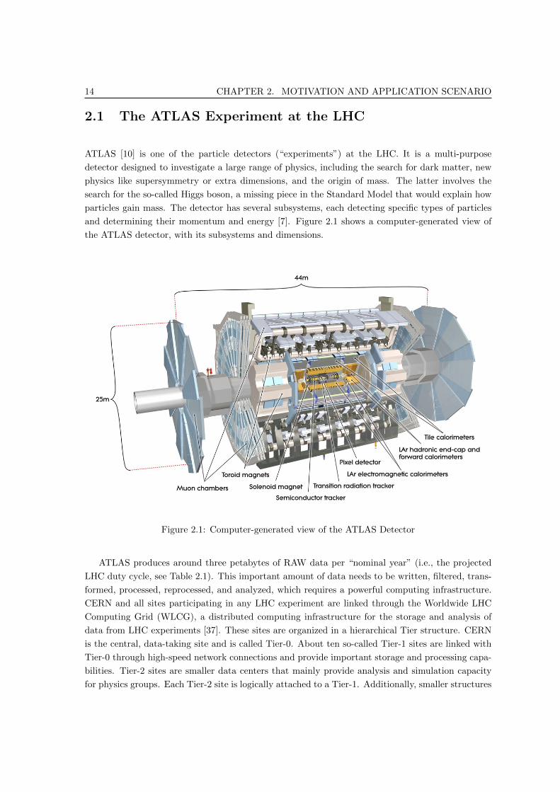
ATLAS [10] is one of the particle detectors (“experiments”) at the LHC. It is a multi-purpose
detector designed to investigate a large range of physics, including the search for dark matter, new
physics like supersymmetry or extra dimensions, and the origin of mass. The latter involves the
search for the so-called Higgs boson, a missing piece in the Standard Model that would explain how
particles gain mass. The detector has several subsystems, each detecting specific types of particles
and determining their momentum and energy [7]. Figure 2.1 shows a computer-generated view of
the ATLAS detector, with its subsystems and dimensions.
Figure 2.1: Computer-generated view of the ATLAS Detector
ATLAS produces around three petabytes of RAW data per “nominal year” (i.e., the projected
LHC duty cycle, see Table 2.1). This important amount of data needs to be written, filtered, trans-
formed, processed, reprocessed, and analyzed, which requires a powerful computing infrastructure.
CERN and all sites participating in any LHC experiment are linked through the Worldwide LHC
Computing Grid (WLCG), a distributed computing infrastructure for the storage and analysis of
data from LHC experiments [37]. These sites are organized in a hierarchical Tier structure. CERN
is the central, data-taking site and is called Tier-0. About ten so-called Tier-1 sites are linked with
Tier-0 through high-speed network connections and provide important storage and processing capa-
bilities. Tier-2 sites are smaller data centers that mainly provide analysis and simulation capacity
for physics groups. Each Tier-2 site is logically attached to a Tier-1. Additionally, smaller structures

2.2. FROM RAW DATA TO EVENT-LEVEL METADATA: TAGS 15
Parameter Value
E (Energy) 14 TeV (two 7 TeV proton beams)
L (Luminosity) 1034 cm−2 s−1 (design luminosity)
Collision rate 109 Hz p-p collisions at design luminosity, resulting from a bunch-
crossing rate of 40 MHz
Trigger rate 200 Hz independent of the luminosity
Operation time 50000 seconds per day
Operation time 200 days per year
Table 2.1: Nominal LHC Operational Parameters and ATLAS Trigger Rate [9].
such as institute clusters are organized in Tier-3 centers. Figure 2.2 [25] shows the Tier structure of
the WLCG sites. At the time of writing, this rather rigid structure is however being rethought by
the ATLAS collaboration.
Table 2.1 summarizes the main LHC and ATLAS operational parameters. In terms of computing
infrastructure, the Trigger rate is the main parameter to consider. ATLAS has a sophisticated trigger
system, consisting of three levels: the Level-1 trigger (LVL 1), based on fast on-detector hardware
components, selects max. 75 - 100 kHz out of the initial 40 MHz bunch-crossing rate. The subsequent
two stages, the High-Level-Trigger (HLT), consisting of the Level-2 trigger (LVL 2) and the Event
Filter, are software-based and run on dedicated online CPU farms; they further reduce the event rate
to several kHz and a nominal rate of 200 Hz respectively. Those 200 Hz of most “interesting” events
are eventually passed to offline processing. While the nominal trigger rate is 200 Hz, higher rates
can be achieved during data taking. For a detailed description of the ATLAS Computing Model the
reader is referred to [9].
2.2 From RAW Data to Event-Level Metadata: TAGs
RAW data from the detector is stored in a byte stream format and transferred from the event
filter to Tier-0, the central ATLAS data processing unit at CERN. At Tier-0, the so-called Tier-0
Management System [38] provides the framework to process the data in several steps, as depicted in
Figure 2.3. First, RAW data are reconstructed to Event Summary Data (ESD), which is intended
to make access to RAW data unnecessary for the bulk of analyses. ESD, as all the subsequently
produced data, is stored in an object-oriented format in ROOT files. Describing ROOT structures is
out of the scope of this work, details can be found in [5]. Analysis Object Data (AOD) is then derived
from ESD, by condensing the quantities most used in physics analysis. In Figure 2.3, temporary
data products (before the merging steps) as well as stored data (right after the merging steps) are
represented. Temporary AOD files are merged into final ones – the merging step reduces the number
of data files. AOD is already more than a factor 10 smaller than RAW data, but still 100 kB in
size per event. In order to allow a rapid filtering of events based on key physics quantities, so-called
TAG files are produced at the end of the reconstruction chain. TAGs are event-level metadata that
contain event descriptors, physics quantities, and sufficient information for back-navigation, i.e.,
for reaching a specific event in upstream data, based on a TAG selection. Table 2.2 summarizes

16 CHAPTER 2. MOTIVATION AND APPLICATION SCENARIO
T0-T1 and T1-T1 traffic Alice
T1-T1 traffic only Atlas
(thick) >= 10Gpbs CMS
(thin) <= 10Gpbs LHCb
TAG site
Figure 2.2: LHC Tier-0 and Tier-1 Sites and Network Overview
the approximate sizes of the main data formats in ATLAS [9]. Note that TAG, like RAW and as
opposed to ESD and AOD, is not an acronym, but is used in analogy to tags, referring to keywords
or metadata related to a piece of information and allowing to search for it.
TAGs are stored as POOL [82] Collections, with a physical back-end either as ROOT files or in
a relational database. The latter are referred to as relational TAGs, as opposed to file-based TAGs.
The Tier-0 management system uploads TAG data from files to several Oracle databases around
the world, making them easily accessible through a services suite. The TAG upload and “posttag
upload” are the last steps of the event reconstruction process at Tier-0, as shown in the top right
corner of Figure 2.3. “Posttag upload” refers to database internal procedures and transformations
applied to TAG data to make them efficiently accessible. An advantage in using databases is the
ability to index the data as required, in order to allow fast and efficient queries.
In the remainder of this work, the focus is put on TAG databases as the source of TAG data.

2.3. TAG DATA AND SERVICES 17
Item Value
RAW Size 1.6 MB
ESD Size 0.6 MB
AOD Size 100 kB
TAG Size 1 kB
Table 2.2: Nominal Event Data Sizes
2.3 TAG Data and Services
In order to gain an understanding of the TAG system and its challenges, it is important to briefly
discuss the content of TAGs, the main use cases and the services provided to enable those use cases.
2.3.1 TAG Content
In a TAG record, an event is described by approximately 300 variables. The TAG content has
originally been defined by a special task force in 2006 [6], and is since then under constant evaluation
by the ATLAS physics and combined performance groups. The aim is to provide content that can
be used for an efficient event preselection and covers all use cases defined by the physics groups.
The exact content is beyond the scope of this overview, but the classes of variables are interesting
to understand the TAG use cases. The variables can be classified as follows.
• Event quantities: include event number, Run number (a run/event number pair uniquely
identifies an event), luminosity block and missing energy values.
• Data quality: bit-encoded words representing error codes per sub-detector.
• Trigger information: bit-encoded word specifying if an event passed a certain trigger or not.
• Number of objects and their properties: number of electrons, photons, muons, jets, etc.
in the event, and basic object properties (e.g., momentum).
• Physics TAG attributes: words for each physics and performance group, free to encode in
a “true/false” manner to mark an event as interesting for a specific analysis.
• Collection information: references to the same event in upstream data products, namely
AOD, ESD and RAW data. These references (called Globally Unique Identifiers, or GUID)
allow for back-navigation to the correct AOD, ESD and RAW file to retrieve the event.
TAGs are write-once, read-many – once written, the content is never updated. If already-
processed RAW data are reconstructed with a new software version and new calibration, a new
version of all data products, including TAGs, is produced. This process is referred to as a Repro-
cessing.
2.3.2 TAG Use Cases
In [32], the role of the TAG database (and more generally the TAG system) is described as “to
support seamless discovery, identification, selection and retrieval of ATLAS event data held in the

18 CHAPTER 2. MOTIVATION AND APPLICATION SCENARIO
merge AODtoAOD
recon RAWtoESD
posttag at DBupload to DB
merge TAGtoTAG
recon ESDtoAOD
merge AODtoTAG
RAW
AOD
TAG
ESD
AOD
TAG
Figure 2.3: Data Reconstruction Chain, from RAW Data to TAGs [8].
multipetabyte distributed ATLAS Event Store.” TAGs are not meant for physics analysis, but for
preselecting interesting events for further analysis. This preselection can be done on any of the TAG
variables. From the selected events physicists can then navigate to the corresponding AOD, ESD or
RAW data, to perform their specific analysis. As this analysis process can be very resource-intensive,
it is preferable to run it only on events that are known to satisfy basic query predicates. An example
TAG query is provided in Equation 2.2.
RunNumber ≥ 52280 AND RunNumber ≤ 52304 AND (2.1)
(LooseElectronPt1 ≥ 20000 OR LooseMuonPt1 ≥ 20000
OR TauJetPt1 ≥ 20000)
According to [6], [30], [31] and recently arisen requirements, the main TAG use cases can be
summarized as follows:
1. Browsing through the TAG data using a web interface (interactive queries). As new collision
2.3. TAG DATA AND SERVICES 19
events are recorded, the TAG database can be used to “check what data is there,” in order to
get a general overview. The TAGs are thus used as an index of the recorded data.
2. Using a TAG selection as input to a physics analysis. For example, let’s consider that all
the TAGs for a specific set of data (ESD, AOD) have been created. A physicist looks at the
TAGs for this entire set of data and finds some interesting classes of events. He then wants to
take the result of this TAG-based preselection and use it as input to a job which looks at the
upstream AOD data. This can mean:
(a) to locally extract a TAG file from the database and use it as input to an analysis job, or
(b) to skim the data and directly get a RAW/ESD/AOD file containing only the events
passing the provided TAG query.
3. Locate events based on a run and event number, and get the corresponding identifiers of the
files containing these events. This functionality is referred to as event lookup and is integrated
into central ATLAS Grid tools.
These generic use cases are addressed by the services of the TAG system, as described in the
following two subsections. More specific use cases continually arise in physics groups, as the analyses
evolve.
2.3.3 TAG Databases
As soon as TAG files are available, their content is uploaded to the TAG databases by the Tier-0
management system, using tools provided by POOL [82]. The TAG databases are relational Oracle
databases. There are several deployments at several tiers of ATLAS, and their federation can
be considered as a distributed database system, as the data can be queried transparently on any
database, using a metadata registry (described in Chapter 4, 4.4).
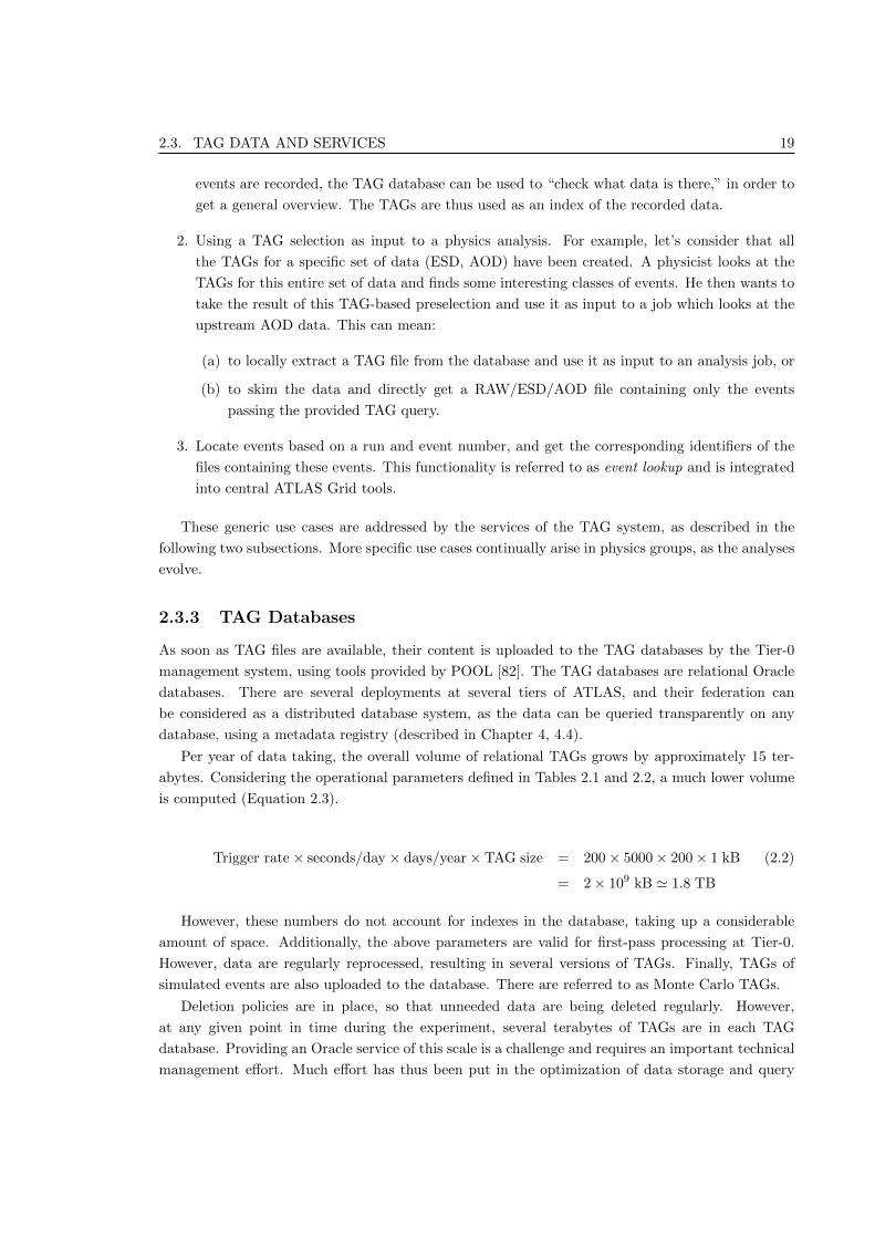
Per year of data taking, the overall volume of relational TAGs grows by approximately 15 ter-
abytes. Considering the operational parameters defined in Tables 2.1 and 2.2, a much lower volume
is computed (Equation 2.3).
Trigger rate× seconds/day × days/year× TAG size = 200× 5000× 200× 1 kB (2.2)
= 2× 109 kB ' 1.8 TB
However, these numbers do not account for indexes in the database, taking up a considerable
amount of space. Additionally, the above parameters are valid for first-pass processing at Tier-0.
However, data are regularly reprocessed, resulting in several versions of TAGs. Finally, TAGs of
simulated events are also uploaded to the database. There are referred to as Monte Carlo TAGs.
Deletion policies are in place, so that unneeded data are being deleted regularly. However,
at any given point in time during the experiment, several terabytes of TAGs are in each TAG
database. Providing an Oracle service of this scale is a challenge and requires an important technical
management effort. Much effort has thus been put in the optimization of data storage and query

20 CHAPTER 2. MOTIVATION AND APPLICATION SCENARIO
management. As part of the posttag process depicted in the right corner of Figure 2.3, TAGs are
indexed, horizontally and vertically partitioned, and compressed.
For details on the operational challenges of the multi-terabyte TAG databases the reader is
referred to [84].
2.3.4 TAG Services
The TAG system is composed of a suite of tightly coupled services, allowing access to TAG data and
supporting the use cases defined in 2.3.2. The main TAG services are listed and briefly described
below, with emphasis being put on providing an overview of the functionality instead of technical
details.
TAG Database. Although being the data source, the TAG database is also considered as a service.
See 2.3.3.
TASK Lookup. Service that allows looking up the TAG registry to locate a given set of data.
TASK (TAG Application Service Knowledgebase) is described in detail in Chapter 4 (Sec-
tion 4.4).
iELSSI. interactive Event Level Selection Service Interface, also referred to as TAG browser. It
is a web interface, implemented using PHP and AJAX technologies, that allows browsing
relational TAG data [107]. It requires a connection to one or more TAG databases and allows
defining queries on all TAG attributes. The attributes are displayed in an ordered manner
mimicking a typical selection process. Based on the entered selection criteria, it allows count
queries and display of results, and can invoke the extract, skim and histogram services defined
below. To properly display and process TAG information, it further uses the trigger decoding,
extract XML builder and Lumiblock range builder services (see below). Figure 2.4(a) shows
an example TAG query entered in iELSSI.
Extract. Service producing a TAG ROOT file containing the specified attributes of the TAGs for
the selected events. The extract service uses POOL [82] utilities wrapped in Python. The
output of extract can be used as input to a local or distributed analysis job, in the latter case
using Grid job submission tools [30]. Extract can be invoked from iELSSI or directly from
the command line, in both cases using an interface defined in XML. Figure 2.4(b) shows the
integration of the extract service in iELSSI (panel “Retrieve without skimming”).
Skimming. Service producing an AOD or ESD ROOT file for the events passing the TAG-based
preselection. The main use case of the skimming service is that of a physicist who wants to first
find interesting events satisfying a specified query, and then run some analysis on those events,
without having to have any knowledge about where these events are, neither in terms of files,
nor in terms of sites hosting the files. Figure 2.4(b) shows the integration of the skimming
service in iELSSI (panel “Retrieve with skimming”).
Event Lookup. The information contained in the TAGs allows determining in which physical
RAW, ESD and AOD file a particular event is residing. As such it is the only event-level file
reference. Event lookup is a service returning the GUIDs of the files containing specific events

2.4. TYPICAL TAG WORKFLOWS 21
provided as input. It is integrated into Grid tools and used for determining the files needed
for an analysis job.
Histogram. Java-based service allowing to draw histograms. It can be invoked from iELSSI and
is used to create histograms displaying TAG variables.
Trigger Decoding. PHP service mapping a trigger name to the appropriate bit in the TAG trigger
words. It is used by iELSSI to decode trigger words inside the TAGs. It can be invoked from
a web browser or with a curl call.
Extract XML Builder. Builds an XML file needed for extract. It is designed to be used by the
command line extract application. It can also be invoked from a web browser or with a curl
call.
Lumiblock Range Builder. Web service that builds the trigger active domain run and lumiblock
range into an XML document. It is designed to be used by any independent application that
needs the run-lumiblock range for its calculations.
runBrowser. Web-based interface that allows users to select runs based on all available conditions
data (data describing the detector status) and conditions metadata [19]. Conditions data refer
to data about the detector status at a given interval in time. The information presented in
runBrowser is an integration of conditions and TAG data.
2.4 Typical TAG Workflows
The services described above are designed to be plugged together in order to build workflows tailored
to allow an event preselection based on TAGs. In general, the input is a user-defined query, and
the output can be a custom TAG or other file, that is then in turn used as input to a detailed
analysis process. Example typical workflows are depicted in Figure 2.4. It shows the user actions
and lists the needed services for displaying events that satisfy a certain user query. The user calls
iELSSI, defines a query based on the available TAG attributes, and finally displays events. If he is
not satisfied with the selection, he can refine the query and display events again, until the selection
is satisfactory. In order to allow for this user workflow, several services need to be instantiated.
First, the metadata registry (TASK) has to be called to locate the data. Second, a trigger decoding
service and iELSSI have to be instantiated, so that the user can define his query. Finally, a TAG
database has to be chosen to run the query on. The second activity diagram on Figure 2.4 shows the
user actions and lists the needed services for extracting TAG data based on a query defined within
iELSSI. An extract query can be spawned over several databases, either because no site hosts the
entire set of required data, or for performance reasons. Several patterns (e.g., sequence, parallelism,
loop) can thus occur in TAG workflows.

22 CHAPTER 2. MOTIVATION AND APPLICATION SCENARIO
(a) iELSSI Query Overview
(b) Extract and Skimming Integration in iELSSI
Figure 2.4: iELSSI Screenshots
2.5 Distribution of Data and Services and Resulting Chal-
lenge
At the time of writing, there are five ATLAS sites acting as TAG sites, four in Europe and one in
Canada. They all host one or more TAG services as defined in Section 2.3.4. More sites are currently
considering joining the TAG project.
Regarding the data distribution, there is a central unit at Tier-0 configuring the TAG uploads
with regards to the sites the data are sent to. The general strategy is to have at least two copies of

2.5. DISTRIBUTION OF DATA AND SERVICES AND RESULTING CHALLENGE 23
Call iELSSI Define Query Review Selection
Selection ok?
yes
no
Extract data Extracted TAG File
Extract TAG data.
Involved services: TASK Lookup, Trigger Decoding, iELSSI, TAG Database, Extract XML Builder, Extract
Display events in iELSSI.
Involved services: TASK Lookup, Trigger Decoding, iELSSI, TAG Database
Call iELSSI Define Query Review Selection
Selection ok?
yes
no
Stored SelectionCount/Display Events
Figure 2.5: Typical TAG Workflows
each set of data for backup purposes, and the latest data available at more sites, because it is queried
most frequently. The distributed TAG databases currently have an overall capacity of 80 terabytes.
Data are grouped in so-called projects and reprocessing passes, and usually a whole reprocessing
set it sent to a site, not only a fragment. However, such a fragmentation can happen and might
even be emphasized in the future, when space limitations arise. A system keeping track of the data
distribution in real time has been implemented in the context of this thesis work. The so-called
TASK - TAG Application Service Knowledge base - is described in detail in Chapter 4 (Section 4.4).
This knowledge base also records all available services, together with monitoring information and
computed metrics. It allows treating all TAG databases as a single distributed database management
system.
TAG sites are hosting other services than the TAG database on a voluntary basis, as resources
are available. The minimum requirement is to have a set of web services per continent, in order not
to suffer from high network latencies. However, it is preferable to have more service deployments,
in order to allow for load balancing and fail-over.
To summarize, the TAG system is composed of several data sources, several abstract services and
one or more concrete deployment(s) per service. All deployments of a service are identical in terms of
functionality and software version, but have different QoS attributes, as they run on heterogeneous
hardware, the hosting sites have different availabilities, different access policies, etc. Figure 2.6 is a
simplified schematic representation of the distributed TAG system.
When a concrete workflow, such as one of the examples described in Section 2.4, is built to
respond to a request, there are thus several choices for composing deployments. The choice of data
sources and service deployments should be made automatically and based on rational decisions,
conforming to the goals stated in Section 1.2 (minimize the response time per request and ensure a
fair and efficient usage of all available resources). As TAG services are getting used more frequently,
since data taking at ATLAS is a continuous process, and an important amount of data are available

24 CHAPTER 2. MOTIVATION AND APPLICATION SCENARIO
Services and QoS Registry
TAG DB
TAG DB
TAG DB
TAG DBTAG DB
TAG Site
TAG Site
TAG Site
TAG Site
TAG Site
Figure 2.6: Distributed TAG System
for analysis, a careful selection of services on a per-request basis is getting crucial in order to ensure
an efficient event selection system based on TAGs. With the current setup, the problem size is rather
small and it might be argued that no specific algorithm or approach is needed to address the service
selection problem. However, the system is expected to grow, both regarding the number of sites
and the number of deployments. Figure 2.5 shows the differences in execution times on the simple
example of composing an iELSSI deployment with a TAG database deployment for an event count
based on the query stated in Equation 2.4. This query is returning 9146 events satisfying the query
out of a total of 36056886 events. CERN refers to the Tier-0 facility, TRIUMF is a data center in
Vancouver, Canada, and RAL is the data center at Rutherford Appleton Laboratory in the U.K.
The Total time is the time in seconds from the query submission to the display of the results in
the IELSSI browser, thus encompassing the query time on the database and the time for sending
the results over the network, building the page, etc. Figure 2.7(a) shows the values measured in ten
subsequent runs with a user at CERN using the iELSSI interface at CERN and varying database
back-ends. The decrease between the first run and the others can be explained by database caching.
It can be seen that the total time when querying the database at TRIUMF is approximately 20 times
higher than when the CERN database is queried, although the two database times (i.e., the actual
query time on the database) do not differ much. The difference thus clearly lies in the link between
CERN and the geographically far away TRIUMF. Figure 2.7(b) allows drawing similar conclusions.
In this test series, the user issuing the query is still at CERN, but accessing iELSSI at TRIUMF.

2.5. DISTRIBUTION OF DATA AND SERVICES AND RESULTING CHALLENGE 25
It can be seen that, although the database time at TRIUMF seems to be higher than at CERN
and RAL, the total time for the combination of the iELSSI at TRIUMF and the TAG Database
at TRIUMF has the lowest total time. In summary, the values show important differences in the
total response times, depending on the invoked deployments. These differences can be explained by
different database server performances, different network latencies due to geographical distances, the
place of the user, and time-dependent factors such as the current load on the invoked resources. A
random or rank-based selection of deployments can thus not ensure an appropriate system response,
making a more sophisticated deployment selection mechanism a necessity.
Collection = data10 7TeV physics Egamma r1774 p327 p333 p372 READ (2.3)
AND RunNumber = 166094
AND NLooseElectron > 1
0
10
20
30
40
50
60
70
80
90
100
1 2 3 4 5 6 7 8 9 10
Tim
e in
se
con
ds
User@CERN, iELSSI@CERN
CERN DB time
CERN total time
RAL DB time
RAL total time
TRIUMF DB time
TRIUMF total time
distinct runs
0
10
20
30
40
50
60
70
80
90
1 2 3 4 5 6 7 8 9 10
Tim
e in
se
con
ds
User@CERN, iELSSI@TRIUMF
CERN DB time
CERN total time
RAL DB time
RAL total time
TRIUMF DB time
TRIUMF total time
distinct runs
(a) User at CERN, iELSSI at CERN0
10
20
30
40
50
60
70
80
90
100
1 2 3 4 5 6 7 8 9 10
Tim
e in
se
con
ds
User@CERN, iELSSI@CERN
CERN DB time
CERN total time
RAL DB time
RAL total time
TRIUMF DB time
TRIUMF total time
distinct runs
0
10
20
30
40
50
60
70
80
90
1 2 3 4 5 6 7 8 9 10
Tim
e in
se
con
ds
User@CERN, iELSSI@TRIUMF
CERN DB time
CERN total time
RAL DB time
RAL total time
TRIUMF DB time
TRIUMF total time
distinct runs
(b) User at CERN, iELSSI at TRIUMF (Canada)
Figure 2.7: Execution Times for Query Involving TAG Database and iELSSI

26 CHAPTER 2. MOTIVATION AND APPLICATION SCENARIO
Before addressing the service selection challenge, several aspects have to be studied and taken
into account:
• What are the components building up the TAG system? How are they mutually related?
• What system QoS attributes can be gathered, and which ones are important to be considered
in the service selection process?
• What are the possible workflows and which patterns do they implement? Based on these
patterns, how are the QoS attributes aggregated?
Chapter 4 addresses those questions, both in a generic way and tailored to the TAG system.
Service selection, and especially web service selection, is a widely studied research topic, and
several approaches have been proposed, as will be discussed in Chapter 3. However, all system
characteristics, requirements and optimization goals have to be studied in detail in order to find an
appropriate solution approach. In particular, it is argued that in an experiment like ATLAS that
is scheduled over several decades, use cases and optimization goals of an event selection system can
change unexpectedly, and the service selection framework has to be able to adapt to these changes.
In this thesis, a detailed study of the service selection problem is carried out, motivated by the
challenges arising in the TAG system. The proposed solution approach is however generic enough
to be applied to other systems.

Chapter 3
Background and Related Work:
Service Selection in Heterogeneous
Environments
Optimizing the selection of things conforming to defined objective functions and satisfying given
constraints is a common and broadly studied problem in many applied research areas such as op-
erations research, production planning, logistics, and many more. In computer science, it arises
for example in the context of scheduling in distributed systems, database query optimization, and
routing in networks. Through all of these examples, while the underlying problem is similar, the
things – i.e., the considered entities to be selected –, the context, the objectives and the constraints
differ. Additionally, depending on the concrete definition and context, the problems can map to
slightly different mathematical models.
QoS-aware service selection is another example of such problems and has recently gained deep
interest with the emergence of distributed, service-oriented systems, in which multiple service in-
stances, differing only in their QoS properties, can be used for a given task in a service chain or
workflow. This chapter defines the basic concepts and investigates related work, in order to pre-
cisely set the problem context and present a state of the art literature survey. While this chapter
sets the basics, related work on more specific concepts used in the course of this thesis is presented
in respective dedicated chapters.
This chapter is organized as follows. Section 3.1 defines the basic concepts used throughout
the thesis. Section 3.2 defines the problem context and setting by comparing it to related prob-
lems. In Section 3.3 models of service-oriented systems and frequently-considered QoS attributes
are discussed. Section 3.4 surveys the most common approaches to solve QoS-aware service selection
problems. Finally, Section 3.5 summarizes research efforts and results in the area of multi-objective
service selection optimization.
27

28 CHAPTER 3. BACKGROUND AND RELATED WORK
3.1 Basic Concepts
Terms like Web Service and Service-Oriented Architecture (SOA) are widespread in the area of
computer science and beyond, but several – sometimes conflicting – definitions exist. It is thus
important to set working definitions in the context of this thesis, in order to precisely state how
the terms are used. To this end, this section provides definitions of basic concepts relevant to the
understanding of this thesis.
Web Service. Although in this thesis we are referring to services in general, not only to Web
services in the strict sense, the term Web service is often used, especially in the context of
related work on Web service selection. The following definition from the World Wide Web
Consortium (W3C) is adopted: “A Web service is a software system designed to support
interoperable machine-to-machine interaction over a network. It has an interface described in a
machine-processable format (specifically WSDL). Other systems interact with the Web service
in a manner prescribed by its description using SOAP-messages, typically conveyed using
HTTP with an XML serialization in conjunction with other Web-related standards.” [101].
Service (extended service definition). In this work, “services” do not strictly refer to Web
services implementing particular standards, but to a software component providing a func-
tionality, independent of its internal realization and interfaces. W3C provides the following
general definition of a service: “A service is an abstract resource that represents a capability
of performing tasks that form a coherent functionality from the point of view of providers
entities and requesters entities. To be used, a service must be realized by a concrete provider
agent.” [101]. A service can thus be a Web service, a Grid service, or an independent piece
of software that can be invoked over a network. For instance, iELSSI as defined in 2.3.4 is
considered as a service.
Service-Oriented Architecture (SOA). A software system composed of several components –
or services – that can act independently or together to provide a defined overall functionality,
is referred to as being service-oriented. In a SOA, the functionality is thus packaged in services,
making the system flexible and reusability of software components easy. W3C provides the
following definition of a SOA: “A set of components which can be invoked, and whose interface
descriptions can be published and discovered.” [101].
Service Selection. In case several concrete services (deployments) exist for a given functionality,
one has to be chosen out of all possible or feasible ones. This requires the ability to determine
what the possible ones are, which is usually done by querying a service registry. The process of
querying a registry and choosing one concrete service (deployment) for a given task according
to some defined criteria is referred to as service selection.
Service Composition. If several services need to be selected to respond to a given request, they
need to be composed in order to operate together. This process involves defining inputs
and outputs as well as exchange formats, i.e., the interoperability between the services has
to be defined and instantiated. Two terms are recurrent in the area of service composition:
orchestration and choreography, as defined below. The Business Process Execution Language
for Web Services (BPEL4WS) is an example of a Web service composition specification.

3.2. OVERVIEW AND COMPARISON OF RELATED RESEARCH AREAS 29
Orchestration. Orchestration defines the sequence and conditions of service invocations and thus
specifies an executable process [70]. It describes the view and control on the overall workflow
from the perspective of one involved party.
Choreography. Choreography defines a collaborative view on a process and enables each party
to describe its part in the interaction [70]. Specifically, a choreography specifies the public
message exchanges between Web services, or between Web service orchestrations.
Workflow. A workflow is a sequence of steps (or services) to be executed. In this context, sequence
does not necessarily mean one after the other, but the steps can be organized in patterns such
as parallel split, exclusive choice, and arbitrary cycles. The concept of workflow patterns is
detailed in [83]. More specifically, the result of a service selection and service composition is
referred to as a concrete or executable workflow. The abstract specification of a sequence of
services is referred to as abstract workflow.
In this thesis, service composition, orchestration and choreography are addressed only implicitly
(because selected services need to actually work together), but the focus is put on the service selection
process, i.e., the step preceding the composition. In the concrete application scenario, the interfaces
between the services as well as the data and control flows are clearly defined and implemented.
Therefore, once concrete service are selected to form a workflow, it is guaranteed that this workflow
can be executed.
3.2 Overview and Comparison of Related Research Areas
In applied computer science, there are several research areas involving combinatorial optimization
problems, such as (Web) service selection, scheduling, query optimization and QoS routing. Ap-
proaches to solve one problem can be applied or at least adapted to another one. The general
problem studied in the context of this thesis is QoS-aware service selection. The three related areas
mentioned above are shortly outlined in the following, and compared to QoS-aware service selection.
Scheduling. In general, scheduling refers to the allocation of limited resources to activities over
time [74]. The term activity can refer to processes and threads, Grid jobs, steps in a produc-
tion process, leisure activities, etc. It is thus a general problem occurring in many different
environments. An activity could also refer to a service in a service selection problem. All the
described scenarios can be viewed as sub-domains of a generic scheduling definition.
Query Optimization. Query optimization is used in Relational Database Management Systems
(RDBMS) to determine the best way to execute a query. The challenge is thus to determine the
most efficient or cost effective Query Execution Plan (QEP) from a multitude of possible QEPs.
A cost-based optimizer parses the input query, generates equivalent expressions, and selects
the expression with minimum costs, according to a cost function. The most common approach
to perform query optimization is dynamic programming [49]. However, alternative approaches
have been proposed, especially in order to address the fact that dynamic programming is
inefficient for optimizing very large queries [49].

30 CHAPTER 3. BACKGROUND AND RELATED WORK
QoS Routing QoS routing is used in IP networks; its goal is to select routing paths based on
QoS considerations. If several alternative paths exist, some can be overloaded and unable to
support QoS requirements, while others have sufficient available resources in terms of network
throughput. According to [44], the goal of QoS routing is to “provide algorithms that are
capable of identifying such paths so as to satisfy the maximum possible number of flows
with QoS requirements.” Decisions about paths can be made based on QoS attributes of the
available network links and on requirements for a given flow or request. The considered system
is thus a network topology, and the QoS metrics relate to network links. The problem maps
to a shortest path problem and approaches used to solve it include Bellman-Ford and Dijkstra
algorithms [44].
The characteristics of the mentioned areas are summarized in 3.1. They present similarities in
their objectives and underlying mathematical models, but differ in their application domains and in
the objects they are operating on. They are clearly related; for instance an algorithmic approach
for solving a QoS routing problem can be applied to service selection with only minor modifications
such as the mapping of variables. In fact, some solution approaches can be found in all these
problem domains. However, each domain also has its own requirements and challenges, beyond the
pure mathematical problem formulation. The problem studied in this thesis qualifies as a service
selection problem. This is thus the topic of the literature review. Establishing a state of the art of
the other areas is beyond the scope of this work.

3.2. OVERVIEW AND COMPARISON OF RELATED RESEARCH AREAS 31
Envir
on
ment
Ob
jects
Resu
ltaft
er
Op
-
tim
izati
on
Math
em
ati
cal
mod
el
Ob
jecti
ves
Web
Serv
ice
Se-
lecti
on
SO
AA
bst
ract
an
d
con
cret
ese
r-
vic
es
Con
cret
ew
ork
flow
MM
KP
,M
CO
PC
on
stru
cta
work
flow
wit
h
max
imiz
edu
tili
tyfu
nc-
tion
wh
ile
mee
tin
gQ
oS
con
stra
ints
.
Sch
ed
uli
ng
Op
erat
ing
Sys-
tem
s,C
lust
ers,
Gri
ds,
etc.
Res
ourc
esan
d
job
s
Job
-to-r
esou
rce
al-
loca
tion
Qu
euin
gth
eory
All
oca
tep
roce
sses
or
job
sto
syst
emre
sou
rces
ina
way
tolo
ad
-bala
nce
the
syst
em
an
dm
inim
ize
reso
urc
est
arv
a-
tion
,w
hil
em
eeti
ng
QoS
con
-
stra
ints
.
Qu
ery
Op
tim
iza-
tion
Dat
abas
eS
ys-
tem
s
Dat
abase
op
era-
tors
Qu
ery
Exec
uti
on
Pla
n(Q
EP
)
Sh
ort
est
path
Det
erm
ine
the
op
tim
al
way
toex
ecu
tea
giv
enqu
ery
on
the
exis
tin
gre
sou
rces
an
d
data
base
ob
ject
s(s
uch
as
in-
dex
es).
QoS
Rou
tin
gIP
net
wor
ks
Net
work
lin
ks
wit
hass
oci
ate
d
QoS
met
rics
Net
work
path
Sh
ort
est
path
,
MC
OP
Imp
rove
per
form
an
cefo
rQ
oS
flow
s(l
ikel
ihood
tob
ero
ute
d
on
ap
ath
cap
ab
leof
pro
vid
-
ing
the
requ
este
dQ
oS
)[4
4].
Tab
le3.1
:C
om
pari
son
of
Rel
ate
dR
esea
rch
Are
as

32 CHAPTER 3. BACKGROUND AND RELATED WORK
3.3 Modeling Service-Oriented Systems
3.3.1 System Models
In general, system models are used to identify and describe the individual components making up a
system. Most authors studying the QoS-aware service selection problem define at least the concept
of a service class and the concept of a service for describing the considered problem space. A service
class allows grouping concrete services based on their functionality. All services inside a service class
have the same functional properties, but differ in their non-functional properties. A service belongs
to exactly one service class, and a service class contains 1 to n services. In some models, for example
as in [56], a service is directly described by the vector of its attributes. The resources on which
services are running are usually not defined. This is due to the fact that most works on the topic
address the problem from the perspective of the service requesters, to whom the actual physical
resources are unknown.
In Zeng et al. [106], the authors propose a service ontology defining the basic concepts used in
their service composition model. (The concept of ontology is studied in Chapter 4.) Organizations
wanting to provide a service have to publish a service description conforming to the agreed ontology.
The authors define a ServiceOntology as a set of concepts (class Concept) used inside a domain and
a set of service classes (class ServiceClass) defining the delivered functionality, i.e., the abstract
services available. A service class is defined by attributes and operations. Relationship types between
service classes include specialization and composition. Non-functional properties of services are
described by quality criteria (class QualityCriterion). Each criterion is defined by a name, a type,
and an expression describing the provenance and computation of the quality attribute. The service
ontology definition is generic, and inside an organization multiple service ontologies can exist and in
turn be shared and composed. To implement the ontology, the authors used IODT, IBM’s Integrated
Ontology Development ToolKit.
Wada, Suzuki and Oba [91] propose a UML profile for modeling non-functional aspects of
service-oriented systems. They define five stereotypes, namely Service, MessageExchange (pair
of request/reply), Message, Connector (connection between two services, including semantics of
message transmission) and Filter (allows customizing the semantics of a message). The authors
present a tool for model-driven development that accepts the proposed UML profile as input and
outputs an application code skeleton. While the model specifies services and message exchange
between them, it does not take into account quality criteria.
Broader, much more complete models have also been proposed. An example is the Common
Information Model (CIM), a standard developed by the Distributed Management Taskforce [35].
The goal of CIM is to provide a common definition and understanding of IT systems, networks,
services, and applications. It allows for extension and therewith enables vendors to exchange in-
formation between systems. It is composed of a Schema containing the model descriptions, and
a Specification providing details about integration issues with other models. The Schema is a set
of UML class diagrams grouped in packages such as System, Database, User, Metrics, and many
others. The level of detail is very high, making it a full reference, but complex to implement. The
Core package defines the basic concepts all other models are derived from. A simplified version of
selected elements of the CIM Core package is depicted in Figure 3.1 [35]. ManagedElement is the

3.3. MODELING SERVICE-ORIENTED SYSTEMS 33
root class from which all others are derived. For instance, a System and a Service are derived from
the EnabledLogicalElement class. CIM provides a detailed, hierarchical representation of a generic
computer system. It is however too complex and detailed for efficiently addressing service selection
problems for which in general a less fine-grained system view is sufficient.
ManagedElement
ManagedSystemElementLocation
PhysicalElementLogicalElement
Job Service ResourcePool System
AdminDomain
EnabledLogicalElement
Figure 3.1: Selected Elements of the CIM Core Model
It has to be noted that in this chapter, when describing related work, the taxonomy originally
adopted by the authors is preserved. In the remainder of this work though, the terms defined in
Chapter 4 will be used exclusively.
3.3.2 QoS Attributes
QoS attributes need to be gathered and analyzed so that they can be used in QoS-aware service
selection optimization. There exists a variety of attributes. In order to determine attributes of a
system, it is useful to rely on a classification that guides through the process of gathering attributes.
CIM [35] contains a type-based model for Metrics. Selected classes of the CIM Metrics schema
are shown in Figure 3.2. In this model, attributes are basically categorized into discrete values
and aggregated values. Classifications of QoS attributes are studied in more detail in Chapter 4
(Section 4.3).
An ontology of QoS attributes, named QoSOnt, has been proposed by Dobson, Lock and Som-
merville in [36]. The authors distinguish two basic classes of QoS attributes, measurable and un-
measurable ones, the former ones having a certain metric. All attributes have a physical quantity of
a given unit, and conversion rates are used for converting values between units. The classes form the
“base QoS” layer of the QoSOnt ontology. In the attributes layer, the authors define QoS attributes
for dependability and performance. The usage domains of the presented ontology are services and
networks in service-centric systems. To show the applicability of the QoSOnt ontology the authors

34 CHAPTER 3. BACKGROUND AND RELATED WORK
developed a tool for service discovery, differentiation and selection.
Papaioannou et al. [68] developed a QoS ontology language for Web services. The ontology
defines a QoS attribute along the following classes of criteria: QoSParameter, Metric, QoSImpact,
Type, Nature, Aggregated, Node and Relationship. All types of QoS attributes are modeled as
sub-classes of QoSParameter. For example, Performance is defined as subclass of QoSParameter,
and has in turn other subclasses such as Throughput. The full taxonomy is however not provided.
Chaari et al. [27] also proposed an ontology of non-functional properties. In their model, non-
functional properties are broadly categorized into QoS properties and context properties. The de-
tailed concepts identified by the authors are represented in Figure 3.3. Further, the authors define
attribute measurement scales: nominal, ordinal, interval and ratio.
It is commonly agreed that QoS attributes are managed inside a so-called QoS registry, where
the available metrics and their values are stored and can be queried at service selection and/or
composition time. An example implementation of such a registry is provided in [63]. The QoS
registry defined and implemented in the context of this thesis is described in Chapter 4 (Section 4.4).
BaseMetricDefinition BaseMetricValue TraceLevelType
DiscreteMetricDefinition MetricDefinition AggregateMetricValue DiscreteMetricValue
ManagedElement
AggregationMetricDefinition
Figure 3.2: Selected Elements of the CIM Metrics Model
QoS attributes are used as input to and as decision variables in QoS-aware service selection prob-
lems. Depending on the considered system, more or fewer attributes can be defined and gathered.
A variety of different QoS attributes are taken into account in related work. The most commonly
considered attributes are summarized in the following:
Execution Time refers to the (estimated) time spent on the execution of a given service (deploy-
ment). It is also referred to as execution duration or as response time. For example considered
in [3, 28, 63, 80, 102, 104, 105].
Costs refer to the amount of money a requester has to pay to the provider for a given service
execution. Also referred to as price. For example considered in [3, 63, 69, 80, 102, 104, 105].
Availability refers to the relative uptime of a concrete service or resource, observed during a defined
period of time. For example considered in [3, 39, 69, 102, 104, 105].
Reliability refers to the probability that a request is correctly answered and processed by a service.
It is the ratio between successful and total executions. For example considered in [3, 39, 69,
80, 105].

3.3. MODELING SERVICE-ORIENTED SYSTEMS 35
Reputation is a measure for the trustworthiness of a service, mainly based on users’ experience
and ranking. For example considered in [3, 63, 80, 105].
Load refers to the utilization of a deployment or resource at a given time t, usually expressed in
percent. For example considered in [28].
Latency expresses the delay in a system, from point A to point B, caused by the network. A
common measure for network latency is the round-trip time, for instance between two servers.
It is the network latency from one server to the other and back. For example considered in [69].
Bandwidth is a bit rate measure of available data communication resources in the network ex-
pressed in bits per second or multiples of it. For example considered in [3].
Throughput refers to the rate of successful delivery of messages over a network, usually expressed
in bits per second or multiples of it. It is determined by the network bandwidth and the actual
load on the network. For example considered in [3, 69].
More QoS attributes are mentioned in literature, but they are usually more complex to deter-
mine and quantify. Examples include security [80], accessibility and regulatory mentioned in [69].
Additionally, attributes based on users’ feedback and ranking can be included into the list of QoS
attributes.
For determining the QoS of a given workflow, the QoS values of the deployments constituting the
workflow in question have to be aggregated. The function behind this aggregation is dependent on
the patterns of the workflow and the nature of the QoS attribute. For example, the costs of a parallel
execution of three deployments is the sum of the costs for each of them, whereas the availability of
the same structure is determined by the deployment having the minimum availability value. Jaeger,
Rojec-Goldmann and Muhl present aggregation functions for several QoS attributes per workflow
pattern in [51]. Workflow patterns and aggregation functions for QoS attributes considered in this
thesis are studied in Chapter 4 (Section 4.3.3).
3.3.3 Motivation for an Ontology for QoS-Aware Service Selection
Although several system and attribute models and ontologies exist in the area of service-oriented
systems (as pointed out in the previous sections), they have not been designed to address QoS-aware
service selection problems in systems comparable to the one studied in this work, which leads to the
following shortcomings when applied to such problems:
• Scope: existing ontologies in the area of Web services, such as the W3C Web Services Architec-
ture Ontology [100], mainly focus on Web service standards and message exchange protocols,
rather than on the underlying basic system architecture, i.e., they are addressing a different
problem domain. An ontology used for service selection problems should specify the compo-
nents needed for the decision on how to build a concrete workflow. In this context, details on
message exchange protocols are out of the scope.
• Level of detail: the level of detail has to be adapted to the scope and application domain. For
example, the Common Information Model (CIM) provides a detailed specification of computing

36 CHAPTER 3. BACKGROUND AND RELATED WORK
Figure 3.3: Classification of Non-Functional Properties by [27]
systems in general. However, the CIM schemas are very detailed, which makes them difficult
to implement. Additionally, they have a much broader focus than the one needed in the
context of service selection problems. For example, details about job configuration are out of
the scope. Some concepts can be reused, but many have to be simplified. Other ontologies on
the other hand lack details needed in service selection scenarios. For example, the ontology
proposed in [27] does not address the question about how to gather, maintain, and update
QoS attributes. The ontology presented in [106] has been designed to address service selection
problems, however in this case the level of detail is rather low, and only a UML class diagram
is provided as specification.
• Application domain: an ontology is usually tailored to a specific application domain. For
example, QoSOnto [36] focuses on dependability attributes in service-oriented systems without
central control instance, i.e., questions regarding compatibility, dependability and comparison
of attributes (possibly provided in different units, depending on the provider publishing the
information) are crucial ones, whereas they are not central in the system considered in this
thesis.

3.4. APPROACHES TO SOLVE THE QOS-AWARE SERVICE SELECTION PROBLEM 37
• Availability: most ontologies are conceptually described, but their concrete specification (e.g.,
in the form of OWL files, cf. Chapter 4 Section 4.2 and Appendix A) is not made available,
making it difficult to reuse and extend them.
For the above-mentioned reasons, and because an ontology should be as simple as possible for its
specific purpose [81], a system and attribute ontology tailored to service selection problems should
be developed. Such an ontology is presented in Chapter 4.
3.4 Approaches to solve the QoS-Aware Service Selection
Problem
A variety of algorithms to address the QoS-aware service selection problem can be found in litera-
ture. This section provides an overview of recurring and widely studied approaches, rather than an
exhaustive list. Figure 3.4 provides a classification overview of the described approaches.
Branch & Bound Graph-based approaches Hybrid Algorithms
Exact Methods Heuristics
Metaheuristics
Evolutionary Computation
Swarm Intelligence Evolutionary Algorithms
Genetic AlgorithmsParticle Swarm Optimization Ant Colony Optimization
Methods for Combinatorial Optimization
Figure 3.4: Overview of Optimization Approaches for Service Selection Problems
3.4.1 Linear Mixed Integer Programming
The general Mixed Integer Programming (MIP) problem can be formulated as [66]:
max{cx+ hy : Ax+Gy ≤ b, x ∈ Zn+, y ∈ Rp+}, (3.1)
where Zn+ is the set of nonnegative integral n-dimensional vectors, Rp+ is the set of nonnegative real
p-dimensional vectors, and x = (x1, ..., xn) and y = (y1, ..., yp) are the variables. An instance of the

38 CHAPTER 3. BACKGROUND AND RELATED WORK
problem is specified by the data (c, h,A,G, b), with c an n-vector, h a p-vector, A an (m×n) matrix,
G an (m× p) matrix, and b an m-vector. All data are assumed in Q. MIP is a mathematical model
seeking at maximizing a given linear objective function while meeting linear constraints. Linear
Programming (LP) is a special case of MIP in which there are no integer variables.
As Web service selection and composition is about maximizing a given utility function (mini-
mizing a function is equivalent to maximizing its negative value) while meeting QoS constraints, it
can be easily modeled as an MIP problem, assuming that the objective and constraint functions are
linear.
For example, Zeng et al. [105] formulate a Web services composition problem and use LP methods
to solve it. In their model, a concrete service composition is represented as an execution plan
instantiating a path in a Directed Acyclic Graph (DAG). Each Web service has a quality vector
associated with it. For each possible execution plan, the aggregated quality vector is computed,
and an optimal plan can be selected based on Simple Additive Weighting (SAW). However, this
method requires that all possible plans are generated. Given N tasks and M potential services for
each task, the resulting computational costs for determining the optimal plan are O(MN ). It is
thus not a scalable approach. Therefore, the authors propose an LP-based technique to select the
optimal plan, without having to actually generate all the possible ones. In the objective function
of the LP problem five QoS attributes (price, duration, reputation, reliability and availability) and
their respective weights are taken into account. Each variable yij has a value of 1 if the respective
service sij is in the selected execution plan, and 0 if not. It thus represents the participation of a
service in a plan. Constraints are formulated on execution duration, price, reliability, availability,
and uncertainty of execution duration. The authors use an LP solver based on IBM’s Optimization
Solutions and Library to solve the stated LP problem. They finally compare the LP-based global
planning approach to local service selection. Global planning results in better overall QoS values,
but the computation costs are slightly higher than for local selection.
While QoS-aware service selection problems can naturally be modeled as MIP problems, compu-
tational complexity and scalability are important issues that can be addressed by hybrid approaches.
Alrifai and Risse [3] also depart from the observation that local service selection, whilst being
efficient, does not allow proper handling of global QoS constraints. They propose a solution that
combines global and local service selection optimization in order to take advantage of the better
QoS results of a global approach and the better performance of a local optimization. To do so,
the authors use MIP techniques. As in [105], the authors model the overall problem as an MIP
problem. Because of the computational complexity that results in poor scalability, they propose
decomposing the problem into two subproblems. In the first phase, the global QoS constraints are
decomposed into local constraints on the component services level and they are sent to the involved
service brokers. In the second phase, each service broker locally selects the best component service
that meets the local constraints. The decomposition of global constraints into local ones is in turn
modeled as an optimization problem, and MIP techniques are used to solve it. The decomposition
aims to find a set of local constraints for each service class, ensuring that the QoS aggregation still
meets all global constraints. This is achieved by introducing quality levels. The computational
complexity of the resulting two-step model is determined by the number of abstract services, the
number of global QoS constraints, and the number of quality levels and does thus not depend on

3.4. APPROACHES TO SOLVE THE QOS-AWARE SERVICE SELECTION PROBLEM 39
the number of available concrete services, which makes the approach scalable. Evaluations show
a significant improvement of the two-step hybrid approach over the global planning in terms of
computation time. The achieved results are close to optimal.
Branch-and-Bound (BB) algorithms are often used to solve IP problems and have been widely
applied to service selection problems. BB is an enumerative relaxation algorithm [66]. Figure 3.5
shows an enumeration tree a BB algorithm operates on. In this simple example it is assumed that
there are three services with two deployments each. Each path from the root element to a leaf
element is a possible composition of services S1, S2 and S3.
root
S1D1 S1D2
S2D1 S2D2 S2D1 S2D2
S3D1 S3D2 S3D1 S3D2 S3D1 S3D2 S3D1 S3D2
S3
S2
S1
Figure 3.5: Total Enumeration Tree for Branch-and-Bound Algorithms
Yu et al. [104] propose BB-based algorithms for service selection both in the sequential flow
and in the general flow model (including parallel and conditional branches). The sequential flow is
modeled as an MMKP as defined in Chapter 1 (Section 1.1). The general flow is modeled as an IP
problem. As BB algorithms are expensive in terms of computation time, heuristic approaches are
also proposed by the authors.
A parallel BB algorithm for the QoS optimization of workflows is proposed in [56]. The authors
also model the QoS-aware service selection problem as an MMKP. They introduce the concept of
a happiness measure to define the user satisfaction with a given workflow. This measure is based
on the aggregation of QoS attributes, and it is the value to be maximized. Solutions to the stated
problem are represented as decision vectors d = (d1, ..., dp), where each dv, v = 1, ..., p corresponds
to a service selected for node v. The workflow structure as well as all available services are provided
as input. The only global variable, lbound, defines the lower bound for the maximal happiness
measure at each state of the algorithm. The happiness measure of each feasible solution constitutes
a lower bound for the optimal happiness. Local solutions are computed on each node without taking
the overall constraints into account, leading to a relaxation of the problem. In the parallel version
proposed by the authors, each node in the decision tree is an instance of the main program and can
be run on a separate Grid node each. A notable speedup is observed for the parallel implementation

40 CHAPTER 3. BACKGROUND AND RELATED WORK
compared to the serial one if the overall computation time is sufficiently large (i.e., the problem
space is above a threshold value) and at least three parallel processes are spawned.
3.4.2 Graph-based Approaches
An abstract as well as a concrete workflow can be represented as DAG. Yu et al. [104] propose
converting an abstract workflow (represented as a function graph) into a service candidate graph
(i.e., a graph with all possible paths to fulfill a given request) as follows [104]:
• every service candidate is a node in the service candidate graph;
• if a link from Fi to Fj exists in the function graph, then from every service candidate for Fi
to every service candidate for Fj there is a link;
• every service candidate v in the graph has a benefit value of Φ and several QoS attributes;
• set network QoS attributes of the links between every two nodes;
• add a virtual source node vs and a sink node vd. vs is connected to all nodes without incoming
links and vd is connected to all nodes without outgoing links. The QoS attributes of these
links are set to zero;
• add QoS attributes of the node to its incoming links and compute the utility of every link.
An example service candidate graph is depicted in Figure 3.6. In this example, there are one to
three concrete service candidates per service class (S1 to S8). One deployment from S3 and one
from S4 are executed in parallel, and either one from S6 or one from S7 is executed (conditional
choice). In the resulting DAG, each edge is associated with a set of QoS attributes and a utility
value. The resulting service selection problem then maps to an MCOP (Multiconstraint Optimal
Path Problem), where the goal is to determine the path from source vs to sink vd reaching the highest
utility value, while meeting all QoS constraints defined in the specific problem setting [104]. The
authors propose a multi-constraint shortest path algorithm to solve the optimization problem. This
algorithm consists of several steps. First, the nodes are ordered topologically. Second, each node is
visited and relaxed. On each node, all feasible paths (i.e., paths meeting all QoS constraints) from
the source to the node are kept in memory. Alternatively, only a certain number of paths are kept,
in order to reduce the memory requirements. The relaxation procedure is listed in Algorithm 1.
The proposed algorithms can be applied to sequential and general flow structures. The general
flow structure includes non-sequential patterns such as parallel and conditional paths. Loops can be
transformed into sequences by unfolding the cycles, given that the number of cycles is known. At
merge nodes, QoS values as well as utility values need to be merged. At parallel merge nodes, since
all services in all branches preceding the join are executed, QoS values need to be aggregated based
on the properties of specific attributes. For example, costs are summed, whereas the minimum of all
availability values is taken, or the maximum of all execution times. At conditional joins, the values
of the chosen branch are propagated.

3.4. APPROACHES TO SOLVE THE QOS-AWARE SERVICE SELECTION PROBLEM 41
vs v3 vd
v1
v2
v5
v4
v8
v6
v7
v9
v10
v11
v16
v17
v18
v12
v13
v14
v15
S1
S2
S3
S4
S5
S6
S7
S8
source sink
Figure 3.6: Service Candidate Graph (General Flow Structure)
3.4.3 Network Topology Approaches
Jin and Nahrstedt [53] studied the service selection problem in large networks. Following the network
nomenclature, the authors call the challenge QoS service routing. The authors define a service path
as an end-to-end network path containing a given service sequence. They further distinguish service
unicast (one-to-one routing scenarios) and service multicast (one-to-many routing scenarios). In the
latter case, multiple end users are receiving data through a workflow, based on individual capacities
and requirements. The authors put an emphasis on the scalability of service routing by adopting a
distributed routing approach. They argue that in the current Web scale, the resulting network is
too big for a centralized monitoring and planning approach.
A hop-by-hop approach is described to address the QoS routing. Each hop sends a QoS probe
message to all the adjacent nodes in a DAG in which the concrete services constitute the vertexes and
the edges are the network links between the concrete services. From all the instances satisfying prior
defined conditions, the one leading to the most delay-efficient service path is selected. Considered
conditions include network bandwidths and machine capacities. The shortest service path is deter-
mined by applying a shortest path algorithm on the DAG. This approach is referred to as Geometric
Location Guided (GLG), as opposed to Local Resource Amplest (LRA). In the LRA approach, the
next hop is the one having the best aggregated QoS value computed based on bandwidth, machine
resources, and machine availability. Because it relies on local heuristics and does not consider lo-
cation information, LRA results in long and inefficient services paths. The authors propose two
combined approaches, namely LRA-GLG and GLG-RLA, differing only in the application order of
the two routing approaches.
Simulations have been carried out to evaluate LRA, GLG and the two combined approaches,
using several metrics such as link utilization, machine utilization and service path length. Results
show that GLG performs best regarding shortest path metrics (as designed), while LRA allows
keeping balanced network and machine loads. In general, over all considered metrics, the best
results are achieved with LRA-GLG.
These results are relevant to the TAG problem setting, as the LRA-GLG approach helps balancing
the tradeoff between path lengths and load balancing in service graphs, which can be mapped to

42 CHAPTER 3. BACKGROUND AND RELATED WORK
Algorithm 1: Relaxation Function of the Multi-Constraint Shortest Path Algorithm
1 µ, v: vertexes on the DAG;
2 Q(p): aggregated QoS of path p;
3 F : utility of edge [µ, v] or path p;
4 P (v): list of paths from the source to node v that satisfy all QoS constraints;
5 if (∃α,Qα > Qαc ) then
6 return
7 end
8 for each p ∈ P (v) do
9 if F(p) > F and ∀α,Qα(p) ≤ Qα then
10 return
11 end
12 if F(p) < F and ∀α,Qα(p) ≥ Qα then
13 remove p from P (v)
14 end
15 end
16 Add path p′ with attributes [µ,Q, F ] to P (v);
minimizing the execution time and maximizing the throughput of the TAG system. However, as
the TAG system has a much smaller scale than the one considered in [53], a centralized global
optimization approach can be adopted.
3.4.4 Game Theory and Bidding
According to [11], “Game theory concerns the behavior of decision makers whose decisions affect each
other.” It analyzes behavior and decision making from a rational point of view and can be applied to
as diverse areas as economics, political science, evolutionary biology, and computer science. In the
latter field, game theoretic approaches have for example been successfully applied to scheduling and
load-balancing problems in Grid computing [59, 78]. Kwok [59] states that as the Grid scales up,
the machines cannot be considered as cooperative anymore, i.e., the peers in a distributed system
might not want to cooperate with each other. The scheduling problem can thus be modeled as a
noncooperative game in which every player independently and selfishly chooses a strategy in order
to optimize its payoff. The payoff is the numerical outcome of the payoff function that maps a utility
to each strategy. The ultimate goal of a noncooperative game is to find an equilibrium, the best-
known being the Nash equilibrium. In this equilibrium state, no player can benefit from changing
its strategy when the other players keep their strategies unchanged.
Game-theoretic models and techniques have equally been applied to QoS-aware service selection
problems [39, 75]. Esmaeilsabzali and Larson [39] study the QoS-aware service selection problem
in a game-theoretic setting from the service provider’s point of view. They model the problem as
a multi-dimensional single-round auction that can be repeated many times. It is multi-dimensional
because several attributes are considered for making a choice. In their study, the authors consider
two quality attributes, namely availability and reliability. Price is considered separately, as a special
attribute. In case there are several providers for a given service, each submits a bid stating the

3.4. APPROACHES TO SOLVE THE QOS-AWARE SERVICE SELECTION PROBLEM 43
proposed price for providing the service. The service requester then selects a bid according to a utility
function depending both on the price and on the advertised QoS attributes. More specifically, service
providers propose a contract defined as 〈qiR, qiA, pi, Ni, fi(t)〉, where qiR and qiA are the minimal
guaranteed values for reliability and availability of service i, respectively, pi is the price, Ni is the
maximum number of requests in a day, and fi(t), 0 ≤ t ≤ 24 is a function specifying the maximum
number of concurrent active services at any given point t in time (hour) per day. A service provider
can only win the contract if he “promises” to fulfill it. The determination of the quality attribute
for the service providers is interpreted as an equilibrium problem, and a dominant strategy that
maximizes the provider’s benefit is derived. The service allocation itself is then modeled as an
auction, and a winner determination algorithm based on dynamic programming is proposed. It is
noteworthy that the winner determination problem can be directly mapped to a knapsack problem,
therefore similar approaches than the ones presented above can be applied.
Shen and Fan [75] motivate the use of a game-theoretic approach by the fact that for time-
sensitive services the waiting time is not only dependent on the provider’s performance, but also
on the number of incoming requests (the queue length), i.e., the selection strategies of all other
system users. Each user thus has to compete with the others for resources. This can be modeled
as a noncooperative game. Based on the observation that pure strategies, i.e., strategies in which
all users tend towards the best evaluated provider, lead to an overload on one or few provider(s)
while leaving others almost idle, the authors propose a cooperative mixed strategy to the service
selection problem. In this strategy, the user selects the service promising the minimum execution
time only with a certain probability. Simulations have been carried out that show that the adopted
approach shortens the average waiting time and queue length, and ensures a load-balancing among
the providers. It is however based on the assumption that the request arrival rate follows a Poisson
distribution.
Cheung et al. [28] propose a bidding-like approach to address load-balancing in service selection
problems. For an incoming request, each service provider hosting a requested service computes a
bid value based on the estimated service time and the current system load. Each provider sends
its bid value to a broker that then selects a concrete service according to a probability distribution.
Experiments show that this approach allows adapting to unexpected load of resources, making it
appropriate for the use in dynamic environments.
3.4.5 Evolutionary Approaches
Evolutionary Algorithms (EA) have been adopted to solve QoS-aware service selection problems [22,
46, 52, 62, 72, 90]. The basic underlying idea is to use evolutionary, mainly genetic, algorithms that
mimic processes from natural evolution to converge a population of possible solutions (i.e., concrete
workflows) to an optimum. As the approach adopted in this thesis is also based on genetic algorithms,
this part of related work is studied in detail in Chapter 6 (Section 6.5), after having defined all terms
and basic concepts needed for a deeper understanding.

44 CHAPTER 3. BACKGROUND AND RELATED WORK
3.4.6 Swarm Intelligence Approaches
Swarm Intelligence is a technique originating from Artificial Intelligence and is concerned with the
design of intelligent multi-agent systems inspired by the social behavior of animals such as ants,
fish, and others [45]. There are two main techniques: Particle Swarm Optimization (PSO) and Ant
Colony Optimization (ACO).
PSO is an optimization method mimicking social behavior of animals or insect swarms [45]. It has
first been introduced by Kennedy and Eberhart [55]. The underlying idea in PSO is that individual
particles of a swarm represent potential solutions to a given problem, much like individuals of a
population in evolutionary algorithms. These particles move through the problem search space by
applying functions taking into account the particles’ position and velocity, allowing them to evolve
towards an optimal or near optimal solution. Specifically, the velocity of each particle is iteratively
modified by its best position found so far, and the best position of its neighbors. Algorithm 2 shows a
simplified PSO algorithm, where xi is the position of particle i, pi denotes its best personal position,
and pg is the best position of particles in its neighborhood [45]. PSO have been applied to many
problems, including scheduling, multi-objective optimization and dynamic problems.
Algorithm 2: Particle Swarm Optimization Algorithm
1 initialize random swarm;
2 repeat
3 for each particle i do
4 if f(xi) ≥ f(pi) then
5 pi ← xi
6 end
7 pg = max(pneighbors);
8 Update velocity;
9 Update position;
10 end
11 until termination condition true;
PSO has recently been applied to QoS-aware service selection problems [54, 79, 102]. In [54], the
authors model a multi-objective service selection problem taking into account cost, time, reputation
and reliability, and design an algorithm based on multi-objective PSO. The approach is compared to
a genetic algorithm and experiments show that the PSO-based approach has an improved runtime
performance. However, no details are provided on the implementation and parameters of the genetic
algorithm. Sun et al. [79] propose a hybrid service selection approach. First, they use fuzzy logic
control to decompose global QoS constraints into local ones, then they perform local optimization
based on PSO. The idea behind this approach is close to the ones presented by Alrifai and Risse
in [3].
The second main technique of swarm intelligence is ACO. ACO algorithms are inspired by the
foraging behavior of ant colonies, characterized by the indirect communication between ants via
pheromone trails that indicate the shortest path between their nest and food sources [45]. Indeed,

3.4. APPROACHES TO SOLVE THE QOS-AWARE SERVICE SELECTION PROBLEM 45
when moving from their nest in order to search for food, ants leave pheromones on their trail. The
ants arriving first at the food source probably took the shortest path, and the probability that they
will choose this same path to return is higher than for any other path. Thus, this trail will have the
highest pheromone concentration, attracting the ants on their next trip for food. The pheromone on
other trails evaporates over time, when no new pheromone is spread there. ACO algorithms mimic
this behavior. Ants represent partial solutions. The central component of the algorithm is the so-
called pheromone model consisting of a set of values. Mathematically, this model corresponds to a
parameterized probabilistic model. In an ACO algorithm, candidate solutions are first constructed
using the pheromone model. Second, these solutions are used to modify the pheromone values
(referred to as pheromone update), in such a way that future solutions are concentrated on promising
areas of the search space, leading to good solutions.
In [94], Wang et al. apply an ACO approach to the service selection problem. The ant nest S is
the virtual start of the service composition, and the food place F corresponds to the last service in
the workflow. The goal is to find the shortest path between S and F , and the ants have to travel to
each service node exactly once. First, every ant calculates a transition probability when moving to
the next service. Second, the pheromone of the path is calculated using a quality function based on
five QoS attributes, response time, price, expire time, availability, and security level. The authors
show that their ACO algorithm reaches at least 95% of the optimum in all their test runs. However,
there is no comparison with a similar approach in terms of runtime scalability. Zheng et al. [108]
also propose an ACO-based approach to the service selection problem, and they include parallel
workflow structures in their model. In their algorithm, ants are initially positioned on the source
vertex of a Web service composition graph defined as a DAG including OR- and AND-vertexes.
Each ant has to find a path from the source to the destination vertex. Specific state transition rules
are applied on OR vertexes, while on AND vertexes ants are cloned so that each path is chosen by
one ant. Local updating rules define how an ant updates the amount of pheromone on visited edges,
and global updating rules are applied once all ants have reached the destination.
3.4.7 Artificial Neural Networks
An Artificial Neural Network (ANN) is an information-processing system inspired by biological neu-
ral networks whose main components are dendrites, soma and axon. An ANN consists of neurons
(processing elements) and weighted connections between them. It is further characterized by its
method of determining the connection weights, and its activation function [41]. ANNs can be ap-
plied to a variety of problems, including pattern recognition and constrained optimization problems.
Figure 3.7(a) depicts a simple ANN consisting of an input layer, a hidden layer and an output layer.
Figure 3.7(b) shows the simplified mathematical model underlying ANN.
ANNs have recently been used to address QoS-aware service selection problems. Cai et al. [20]
design a neural network predicting controller that evaluates all possible service candidates according
to knowledge from previous selections, service attributes, and context information. Four objectives
are defined: maximize the performance from the client’s perspective, while satisfying QoS require-
ments; maximize the service efficiency and load balancing; minimize the jitter, delay and packet loss
in the network; and minimize the time spent in the application. The results of the evaluation are
then transferred to a service selection controller that selects the actual best service and returns it

46 CHAPTER 3. BACKGROUND AND RELATED WORK
to the client. For the evaluation, a Back Propagation ANN is used, consisting of multiple inputs,
one hidden layer, and a single output (the result of the evaluation function). All factors affecting
the evaluation are used as input. Four kinds of input variables are considered: status parameters
of the affected servers (use of memory, CPU, etc.), status parameters of the network (network load,
bandwidth, etc.), collected parameters from past executions, and reliability measures. The authors
name the following advantages in using an ANN for their service selection problem: ability to in-
clude context information, ability to include information from previous selections and compositions,
scalability and efficiency. The proposed approach has been implemented and evaluated in an ubiqui-
tous Web services environment. Simulations show, among other results, that the proposed approach
outperforms two comparable approaches (one based on genetic algorithms and fuzzy logic, and one
based on trust mechanisms) in terms of service selection reliability.
Al-Masri and Mahmoud [1] use Back Propagation ANNs to classify services into categories (Plat-
inum, Gold, Silver, Bronze), based on their QoS attributes such as response time, throughput, avail-
ability, and reliability. As above, one hidden layer is used, and sigmoid activation functions are
defined for the neurons. An evaluation has been carried out based on a publicly available collection
of QoS metrics of real Web services. Simulations were run to determine the best network configu-
ration. The configuration leading to the highest performance rate (defined as the ratio of correctly
classified services to total services) has then been used for training the network and running fur-
ther tests. The authors note that the learning rate and the number of nodes in the network are
crucial values that impact the system performance. It has further been observed that the more
QoS parameters are taken into account, the higher the performance of the ANN. No comparisons to
other approaches have been carried out. The authors conclude that the proposed ANN is capable
of correctly classifying Web services in a ranked manner, based on published QoS attributes.
x1
x2
xi
z1
z2
z3
zp
y1
yj
s fz y
x1
x2
xn
w1
w2
wn
xi inputswi weightss input functionz net inputf activation funtion y output
Input layer Hidden layer Output layer
(a) Multilayer ANN
x1
x2
xi
z1
z2
z3
zp
y1
yj
s f z y
x1
xn
w1
w2
wn
xi inputs
wi weights
s input function z net input f activation funtion y output
Input layer Hidden layer Output layer
x2
(b) ANN Mathematical Model
Figure 3.7: ANN Components and Simplified Mathematical Model

3.5. MULTI-OBJECTIVE SERVICE SELECTION OPTIMIZATION 47
3.5 Multi-Objective Service Selection Optimization
Service selection problems, as many other optimization problems, can have more than one objective
function. Objectives are usually competing, i.e., the best solution with regards to one objective
can be the worst with regards to another objective. A good solution is thus a compromise between
the various objectives. For example, in a service selection scenario one might want to minimize the
expected execution duration while also minimizing costs. Assuming that better performing services
cost more than less performing ones, a decrease in execution time will result in an increase of the
related costs. These problems are referred to as Multi-Objective Optimization Problems (MOOP)
and are discussed in Chapter 5 (Section 5.4). In the following, recurring competing objectives and
approaches to solve MOOP in service selection scenarios are briefly outlined.
Several authors formulated specific service selection challenges as multi-objective optimization
problems [62, 72, 90]. Liu et al. [62] describe a scenario with two objectives, namely minimizing the
execution time and minimizing the costs, and impose constraints on reliability and reputation. The
authors propose a strategy for global optimization of dynamic Web service selection based on a multi-
objective genetic algorithm. Qiqing et al. [72] aim at finding a concrete workflow that minimizes
cost and time, and maximizes the overall reliability while meeting user-defined QoS constraints.
To address this multi-objective optimization problem, they propose a Multi-Objective Ant Colony
Optimization (MOCACO) algorithm. The authors compare their algorithm to a multi-objective
genetic algorithm proposed in [62] and show that, for different test settings, MOCACO outperforms
the GA both in runtime performance and in the solution quality. An evolutionary approach is
also presented in [90], where minimizing costs and maximizing throughput are the two competing
objectives.
Yu and Bouguettaya [103] propose using multi-objective optimization techniques to compute
service skylines. A service skyline is a small set containing the best services regarding defined
criteria. The aim is to return to the user a set of services that satisfy his requirements and represent
good (non-dominated, cf. Chapter 5, Section 5.4) solutions to multiple objective functions. This
way, the user can himself choose a service, but is not confronted with the whole set of available ones.
The concept of a service skyline is inspired from the concept of top-k queries in database systems.
Related work on multi-objective service selection optimization using EA is studied in more detail
in Chapter 6 (Section 6.5).

48 CHAPTER 3. BACKGROUND AND RELATED WORK

Chapter 4
An Ontology of Components and
Attributes of Distributed,
Service-Oriented Systems
Many modern computing systems, be they for scientific or business applications, are designed as
service-oriented systems, i.e., self-contained pieces of functionality are provided in individual services
that can act independently or together. Additionally, for performance, scalability, and reliability
reasons, they can be distributed across geographical sites and even organizational boundaries. In-
deed, components of a service-oriented model can be easily distributed due to their self-containment.
However, such a system also requires a high level of management, in particular if the distributed
units are heterogeneous, i.e., not necessarily pure standard-conform Web services that are described
in a SOAP interface and can be discovered via UDDI. Therefore, it is important to have a mech-
anism to describe and monitor such systems. To this end, this chapter presents a system and
attribute ontology and classification. Its purpose is to identify the building blocks of heterogeneous,
service-oriented systems and the attributes characterizing those blocks. The proposed models are
customized to the TAG system, showing their applicability to a real-world example. Finally, a con-
crete implementation of a service registry – the so-called TAG Application Service Knowledge Base
(TASK) – is described.
This chapter is organized into sections as follows. In Section 4.1 the purpose and scope of on-
tologies are outlined, and the methodology adopted in this chapter is described. Section 4.2 presents
the generic system ontology and its application to the TAG system, defining the individual system
components and their interactions. In Section 4.3 system attributes, specifically QoS attributes,
are studied in detail. A QoS attribute taxonomy is presented and applied to the TAG system, and
attribute aggregation functions are defined. Section 4.4 details design and implementation consid-
erations of TASK. Finally, Section 4.5 summarizes the key notions and concludes this chapter.
49

50 CHAPTER 4. AN ONTOLOGY OF SYSTEM COMPONENTS AND ATTRIBUTES
4.1 Methodology
Many different parties are usually involved in the design, implementation, operation and support
of a large-scale, distributed system. In the TAG use case for example, system engineers and de-
velopers are members of the ATLAS collaboration, working in different countries, time zones, and
institutions, although all belonging to the same Virtual Organization (VO), namely ATLAS. The
collaborative aspect and efficient communication structures thus play an important role. Addition-
ally, all contributed pieces of software have to work together. This is referred to as an interoperability
requirement. It is thus crucial that all involved parties have a common understanding of the system
and its scope and building blocks as well as their interactions. Therefore, it is beneficial to build
and agree on a system model and related vocabulary. This eases communication and future software
contributions as well as the adoption of optimization strategies on the existing system.
Ontologies are a means to achieve the above stated goals. An ontology is a shared understanding
of a domain of interest, generally viewing this domain as a set of concepts, their definitions, and
their inter-relationships [81]. It defines a structured namespace built upon hierarchies that sets
the semantics of the system it has been designed for. Its primary benefit is to define a common
vocabulary that has to be used by all those interacting with the system. The benefits of defining
and using ontologies in the area of service-oriented systems and service selection have been pointed
out by Yu and Bouguettaya [103] in their work on foundations for an efficient selection of Web
services. The authors characterize an ontology as shared (i.e., the involved parties have to agree on
it), explicit (i.e., all terms are explicitly defined) and formal (i.e., described in a well-defined and
unambiguous model or specification language). The definition and representation of an ontology
range from a simple classification to a fully axiomatized theory, each providing a different level of
formality. Uschold and Gruninger [81] propose four degrees of formality an ontology can provide:
1. highly informal : expressed loosely in natural language.
2. semi-informal : expressed in a restricted and structured form of natural language.
3. semi-formal : expressed in an artificially defined language.
4. rigorously formal : precisely defined terms with formal semantics, theorems and proofs of, for
example, soundness and completeness.
Ontologies are used in several different communities, and they are a central part in many kinds
of applications, such as knowledge portals, information management systems, and semantic Web
services [77].
As pointed out in [81], there are three main areas that can benefit from an ontology: communi-
cation, interoperability and systems engineering, as depicted in Figure 4.1. Those three areas are of
central interest in distributed, service-oriented systems. First, it is all about engineering a system
composed of services acting as autonomous, high-level building blocks. Second, those services are
required to operate together, often across organizational boundaries. Third, the involved organiza-
tions and their people need to communicate in order to develop and deploy inter-operable services.
Ultimately, the goal is to compose those services together in order to fulfill a complex workflow. As
shown in Chapter 2, this is in particular a requirement of the TAG system.
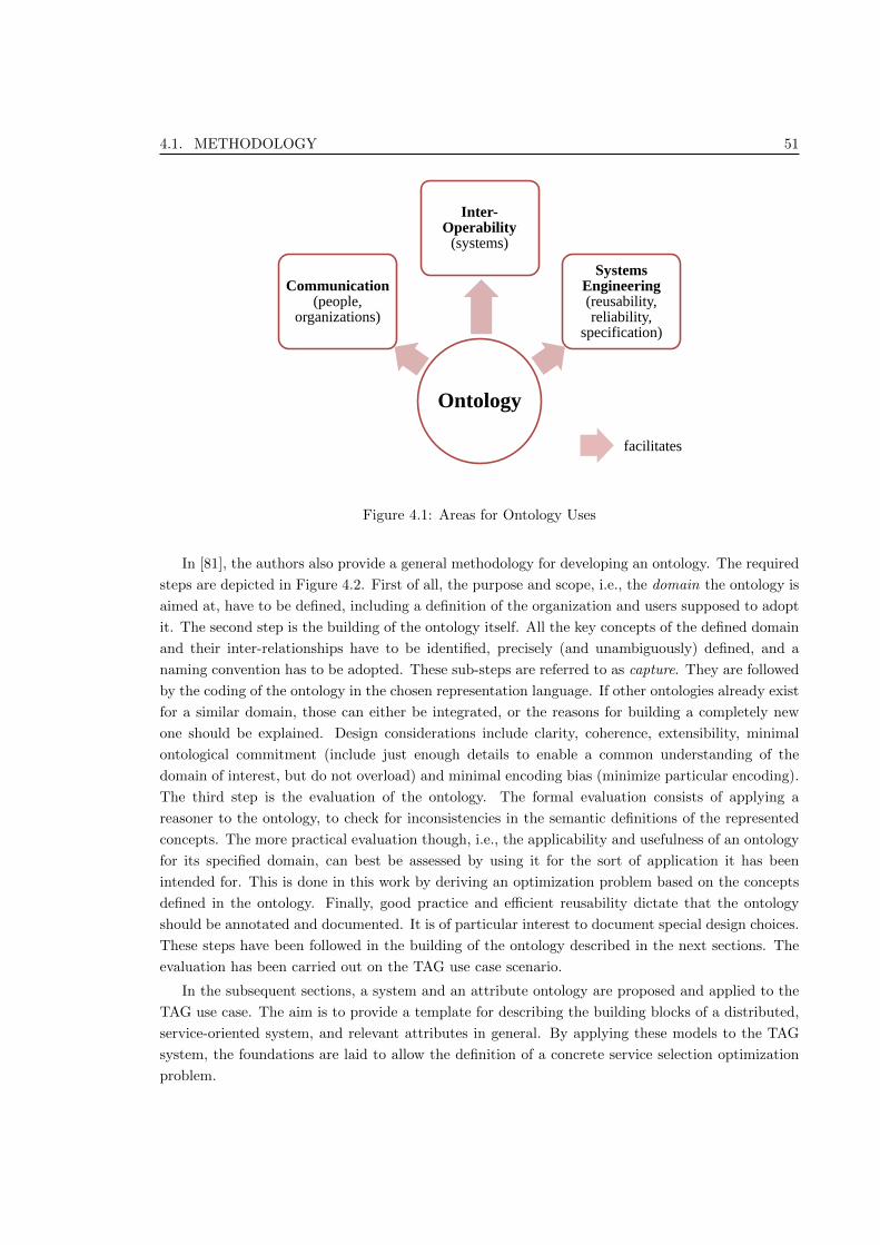
4.1. METHODOLOGY 51
Ontology
Communication(people,
organizations)
Inter-Operability
(systems)
Systems Engineering (reusability, reliability,
specification)
facilitates
Figure 4.1: Areas for Ontology Uses
In [81], the authors also provide a general methodology for developing an ontology. The required
steps are depicted in Figure 4.2. First of all, the purpose and scope, i.e., the domain the ontology is
aimed at, have to be defined, including a definition of the organization and users supposed to adopt
it. The second step is the building of the ontology itself. All the key concepts of the defined domain
and their inter-relationships have to be identified, precisely (and unambiguously) defined, and a
naming convention has to be adopted. These sub-steps are referred to as capture. They are followed
by the coding of the ontology in the chosen representation language. If other ontologies already exist
for a similar domain, those can either be integrated, or the reasons for building a completely new
one should be explained. Design considerations include clarity, coherence, extensibility, minimal
ontological commitment (include just enough details to enable a common understanding of the
domain of interest, but do not overload) and minimal encoding bias (minimize particular encoding).
The third step is the evaluation of the ontology. The formal evaluation consists of applying a
reasoner to the ontology, to check for inconsistencies in the semantic definitions of the represented
concepts. The more practical evaluation though, i.e., the applicability and usefulness of an ontology
for its specified domain, can best be assessed by using it for the sort of application it has been
intended for. This is done in this work by deriving an optimization problem based on the concepts
defined in the ontology. Finally, good practice and efficient reusability dictate that the ontology
should be annotated and documented. It is of particular interest to document special design choices.
These steps have been followed in the building of the ontology described in the next sections. The
evaluation has been carried out on the TAG use case scenario.
In the subsequent sections, a system and an attribute ontology are proposed and applied to the
TAG use case. The aim is to provide a template for describing the building blocks of a distributed,
service-oriented system, and relevant attributes in general. By applying these models to the TAG
system, the foundations are laid to allow the definition of a concrete service selection optimization
problem.

52 CHAPTER 4. AN ONTOLOGY OF SYSTEM COMPONENTS AND ATTRIBUTES
Define the purpose and scope of the ontology
Build the ontology:
Capture
Coding
Integration
Evaluate the ontology
Document the ontology
Figure 4.2: Methodology Applied for Building the Ontologies
4.2 System Ontology
The system ontology defines the building blocks of a distributed, service-oriented system, and is in
particular applied to the TAG system.
4.2.1 Generic System Ontology
For building the ontology, the methodology outlined in Section 4.1 has been followed.
Domain, Purpose and Scope. The purpose of the ontology is to determine and define the high-
level building blocks of a distributed, service-oriented system (in the following, the term system
refers to distributed, service-oriented system – a definition of the term is part of the ontology).
The domain of the ontology are systems, independent of their content and application area.
It is thus about how a system is built, not what it is for and what can be achieved with it.
The ontology aims at easing the documentation, extension and operations of such a system.
First, by providing a model of a computing system and naming all its components and possible
relationships, it can be used as a template for representing and documenting a concrete system.
Second, when a developer provides a new piece of software, the ontology helps to integrate it
into the existing infrastructure. Finally, knowing the building blocks and their characteristics
and properties eases the operations, configuration, and incident detection. Questions being

4.2. SYSTEM ONTOLOGY 53
addressed by the ontology include:
• What are the components of a system?
• Which logical components run on which physical components?
• What are the attributes describing each component?
• Which attributes should be included in the service selection process?
Ultimately, the ontology allows identifying the objects and attributes to consider in the service
selection optimization process. This will be demonstrated on the example of the TAG system.
Users of the ontology include software developers and people ensuring the operations of a
system. The ontology is supposed to be maintained by system managers.
Building the Ontology. The ontology building consists of the following three steps.
Integration. The integration has been discussed in Chapter 3, Section 3.3.3.
Capture. The identified classes, object properties, and data properties are summarized in Ta-
bles 4.1 and 4.2 and depicted in Figures 4.3 (inferred class hierarchy view from Protege 1,
only the relevant classes are shown unfolded) and 4.4 (graphical representation with On-
toGraf, a built-in representation tool in Protege).
Coding. The ontology has been implemented using the Web Ontology Language (OWL),
using the Protege toolkit [77]. An overview of the OWL concepts and constructs used
to build the ontology is provided in Appendix A.1. The full OWL file is provided in
Appendix A.2.
Evaluation. The ontology has been checked for semantic errors using the Protege plug-in reasoner
HermiT 1.3.4. The practical evaluation is carried out on the TAG system. The resulting
TAG system model is described in Section 4.2.2.
Documentation. There has been no distinction (in terms of classes) made between a physical and
a logical component, because this does not add any relevant information for the domain of
discourse and its purpose (for example, logical and physical components can have similar QoS
attributes, thus no distinction is required). Provider is a defined class, because anything
that hosts at least one resource (cardinality restriction) can be considered as a provider in the
system. Deployment is a defined class, because anything that has the relation isDeploymentOf
to a resource and a service is necessarily a deployment. Per definition, a deployment can have a
single isDeploymentOf relation, the range being a resource and a service. An individual of the
class Link has to link (property links) at least two individuals, one of the class Link to one of
the classes Provider, Resource, or Deployment. This is defined so vaguely in order to allow
choosing at which level links are defined. For example, if a provider is defined more precisely as
a site (as in the TAG context), a link can be defined between two providers, which is a rather
generic definition, or between two deployments, which is much more precise, but on the other
hand can constitute quite a documentation overhead in a large system. For example, in the
1Acknowledgment: This work was conducted using the Protege resource, which is supported by grant LM007885
from the United States National Library of Medicine.

54 CHAPTER 4. AN ONTOLOGY OF SYSTEM COMPONENTS AND ATTRIBUTES
TAG system links will be defined at the provider level. However, network connections inside
a provider can be quite heterogeneous, thus this abstraction removes some precision from the
model. A Link is also a defined class: any individual in the system that links at least two
components necessarily belongs to the class Link. AtomicComponent and ComposedComponent
are disjoint defined classes. Each individual from the class SystemComponent has to have
the functional data property isAtomic – an AtomicComponent has isAtomic set to true, a
ComposedComponent has it set to false. What a ComposedComponent is really composed of
is out of the scope here, because it is assumed that only components relevant for the service
selection optimization are documented. But the ontology can easily be extended, by stating
that each composed component has to be composed of another system component from the
same type (i.e., a resource can only be composed of another resource, etc.).
Figure 4.3: Generic System Ontology: Inferred Class Hierarchy
4.2.2 Application: TAG System Components
The components of the TAG system are described in accordance with the ontology defined above.
Figure 4.5 shows the derived UML class diagram, and each component is described in the following.
Provider (Site). A Provider is also named Site in the TAG context. It refers concretely to a Tier of
ATLAS hosting at least one deployment of a TAG service. Among the TAG sites, there are both
Tier-1 and Tier-2 sites. For information on ATLAS Tiers, the reader is referred to Chapter 2
(Section 2.1) and to the Glossary (Tier). Examples of TAG sites include CERN, TRIUMF
(Vancouver, Canada) and DESY (Hamburg, Germany). A concrete provider Pi, i ∈ {1, ..., nP }

4.2. SYSTEM ONTOLOGY 55
Name Description
Thing Root Class in OWL.
System A computing system composed of several components that can act to-
gether to provide some defined functionality to users interacting with
the system, be they humans or other systems.
SystemComponent Logical or physical building block of a system.
AtomicComponent
(defined class)
Component that, in the context of the ontology, cannot be further de-
composed into smaller components.
ComposedComponent
(defined class)
Component that, in the context of the ontology, is composed of at least
two individuals of the class AtomicComponent.
Provider
(defined class)
(Virtual) organization hosting at least one resource that is part of the
system of interest. In the studied context in particular, there is only
one virtual organization (ATLAS), and the generically defined provider
maps to a site. Therefore, in the following the term site is used, referring
to a physical organization hosting at least one resource.
Resource
(defined class)
Physical or logical entity capable of hosting a service. Examples in-
clude web servers, database server or virtual machine. Resources can be
nested, e.g., a virtual resource can run on a physical resource.
Service Abstract, self-contained functionality that can be provided as a piece of
software or a standalone application and that might be composable with
other services.
Deployment
(defined class)
Instance of a service running on a resource. It is a concrete piece of
software that can be invoked over the network.
Link
(defined class)
Network connection between two physical system components allowing
access from component A to component B. It is defined on the compo-
nent level, because depending on the aimed granularity it can be defined
between sites, resources, or deployments.
Attribute Thing describing (characterizing) a SystemComponent functionally or
non-functionally. The concept of attributes is developed in detail in
Section 4.3.
Table 4.1: System Ontology: Classes

56 CHAPTER 4. AN ONTOLOGY OF SYSTEM COMPONENTS AND ATTRIBUTES
Name Description
consistsOf Is the relation between System (domain) and SystemComponent (range).
A system consists of several components that can in turn be services,
resources, etc. The inverse property is constitutes.
hosts Is the relationship between a Provider (domain) and a Resource
(range). An individual has to host at least one resource belonging to
the system for qualifying as provider/site. This is a necessary and suffi-
cient condition. The inverse is isHostedBy
hasDeployment Is the relationship between Resource AND Service (range) and
Deployment (range). Each deployment has exactly one inverse prop-
erty, namely isDeploymentOf, to a resource and a service.
links Is the relationship between a Link (domain) and either a Provider or
a Resource or a Deployment (range), generally describing a network
connection. It is a symmetric property, i.e., acting in both directions.
hasAttribute Is the relationship between any SystemComponent and an individual of
the class Attribute. The inverse is isAttributeOf.
hasName Data property that assigns a name to a SystemComponent.
hasID Data property that assigns a unique ID to a SystemComponent.
isAtomic Is a functional data property with two possible values (true, false)
specifying whether a component is atomic or composed. In the latter case
it can be decomposed into atomic components. This property defines the
disjoint classes AtomicComponent and ComposedComponent.
Table 4.2: System Ontology: Properties

4.2. SYSTEM ONTOLOGY 57
Figure 4.4: Generic System Ontology: OntoGraf Representation
is defined as:
Pi = {id(Pi), [pi1 , ..., pik ]} (4.1)
where id(Pi) is a function associating a unique identifier, and [pi1 , ..., pik ] is the vector of
k attributes associated to the provider (via the property hasAttribute in the ontology).
P := P1 ∪ ... ∪ PnPis defined as the union of all providers or sites, where nP = |P | is the
number of providers in the system.
Service. The TAG services are described in Chapter 2 (Section 2.3.4). Formally, a service Si, with
i ∈ {1, ..., nS}, is described using a unique identifier: Si = id(Si). S := S1 ∪ ... ∪ SnSis the
union of all services and nS = |S| is the number of services in the considered system.
Resource. In the TAG context, resources include database servers and web servers. Database
servers at sites host the TAG database, and web servers host the other TAG services, such
as iELSSI and Trigger Decoding. A resource is owned by and hosted at a site (provider). A

58 CHAPTER 4. AN ONTOLOGY OF SYSTEM COMPONENTS AND ATTRIBUTES
TAGResource
+resourceID+resourceName
1 *consistsOf4
is-a
TAGService
+serviceID+serviceName
is-a
TAGDeployment
+deploymentID+deploymentName
1 1
0..* 1..*
3 hasAttribute
Link
+linkID+linkName
TAGSite
+siteID+siteName
TAGSystemComponent
+componentName+componentType
Attribute
+attributeName+attributeType
TAGSystem
is-a
1*hosts4
2* links
NonFunctionalAttribute
Figure 4.5: TAG System Model (UML Class Diagram)
concrete resource Ri, i ∈ {1, ..., nR} is defined as:
Ri(Pj) = {id(Ri), Pj , [ri1 , ..., ril ]} (4.2)
where id(Ri) is a function associating a unique identifier to the resource and [ri1 , ..., ril ] is the
vector of l attributes associated with the resource. As shown in Equation 4.2, the belonging
to a provider is part of the resource definition. According to Equation 4.1, this is equivalent
to:
Ri(Pj) = {id(Ri), {id(Pj), [pj1 , ..., pj1 ]}, [ri1 , ..., ril ]} (4.3)
R := R1 ∪ ... ∪ RnRis defined as the union of all resources, where nR = |R| is the number of
resources in the considered system.
Deployment. A deployment is an instance of a TAG service on a TAG resource. For example,
“iELSSI@CERN” is a deployment of the IELSSI service running on a specific web sever at site
CERN. Formally, a deployment Di(Sj), i ∈ {1, ..., n} is defined as:
Di(Sj) = {id(Sj), {id(Di), [di1 , ..., dim ]}} (4.4)
where id(Di) is a function associating a unique identifier to the deployment and [di1 , ..., dim ]
is the vector of m attributes associated with the deployment. As suggested in Equation 4.4
the service that a deployment is associated with is part of its definition. D := D1 ∪ ... ∪DnD
is the union of all deployments, where nD = |D| is the total number of deployments in the
considered system.

4.3. ATTRIBUTE ONTOLOGY 59
Link. In the generic model, a link can be defined between any components. In the concrete TAG
example, for simplicity and as a first approximation, a link is defined as the network connection
between two sites (providers). Defining a link between two resources might be more accurate,
but also requires more complex documentation and network monitoring. Formally, a link
Li, i ∈ {1, ..., n} is defined as:
Li(Pj , Pk) = {id(Pj), id(Pk), [li1 , ..., lin ]} (4.5)
where id(Pj) and id(Pk) refer to two sites linked by Link Li and [li1 , ..., lin ] is the vector
of n attributes associated with the link. L := L1 ∪ ... ∪ LnLis the union of all links, and
nL = |L| = |P | × (|P | − 1)/2 is the number of links in our system, assuming that no self-links
are considered.
Attribute. An attribute of component i is defined as:
qi = {id(qi), Dom(qi), Tgt(qi)} (4.6)
where id(qi) is a function associating a unique identifier to the attribute, Dom(qi) is the
Definition Domain and Tgt(qi) is the Target Domain of qi, i.e., the set of all values ai taken
by the attribute.
4.3 Attribute Ontology
As presented in Chapter 3 (Section 3.3.2), many different non-functional attributes are considered
in related work on specific service selection problems. Often, a few attributes are given as examples,
but it is not clear whether others could be gathered and analyzed, and might have an impact.
Additionally, attributes can be very different from each other, due to different units, dimensions,
or to the way they are determined. Based on these observations and on the analysis of the related
work in the area of QoS attributes in service-oriented systems, an attribute ontology is proposed.
Its aim is to provide a high-level framework for classifying QoS attributes, and it thus helps both to
identify and to precisely define them.
4.3.1 Generic Attribute Ontology
In the system ontology described in Section 4.2, a class named Attribute has been introduced.
Individuals from the class SystemComponent are related to individuals from Attribute via the
property hasAttribute, that can also be expressed as “characterized by”. The attribute ontology
refines the Attribute class, both in terms of semantics (what does the attribute express) and
syntactics (how is the attribute value constructed).
Domain, Purpose and Scope. The domain of the ontology are non-functional attributes char-
acterizing the components of distributed, service-oriented systems. Its purpose is to provide
a framework for classifying such attributes, describing their structure, and specifying whether
they are used in the deployment selection optimization process.

60 CHAPTER 4. AN ONTOLOGY OF SYSTEM COMPONENTS AND ATTRIBUTES
Building the Ontology. The ontology building consists of the following three steps.
Integration. The integration has been discussed in Chapter 3, Section 3.3.3.
Capture. The identified classes and properties are represented in Figures 4.6 and 4.7 and
described in detail below.
Coding. The attribute ontology has been implemented in Protege in the same OWL file as
the system ontology presented above. The full OWL file is available in Appendix A.2.
Evaluation. In the same way as for the system ontology, the model has been checked with the
Protege built-in reasoner HermiT 1.3.4 and the applicability is studied on the TAG system,
as described in Section 4.3.2.
Documentation. Design considerations are detailed in the description of the classes and properties
below.
The following base concepts have been identified as classes in the ontology:
AttributeMetaData regroups metadata of attributes used to identify them. For example, an indi-
vidual from the class Attribute should have a name and a unique identifier inside a system,
so that it can be unambiguously referred to.
AttributeValueDataType is a class regrouping all possible data types that an attribute value can
assume. Examples include integer, float, boolean, string, etc.
AttributeValueType regroups subclasses of types of values that attributes can assume, i.e., abso-
lute or relative. The class AbsoluteValueType defines absolute values that can be for example
defined and set, measured, or estimated. A RelativeValueType is a QoS value that is defined
in scales instead of absolute values, such as “low-medium-high”. For example, for the Amazon
Elastic Compute Cloud (Amazon EC2) service, instance types are defined in the following
categories: small, large, and extra large [4]. Moreover, attributes related to privacy and se-
curity can hardly be expressed in absolute values, but they can be rated for instance as low,
medium and high. Attributes resulting from user-rankings also usually fall into this category.
RuleValueType is an attribute type for non-numerical attributes, for example for regulatory
attributes expressing the compliance to a certain law. In such a case, the value cannot be a
simple number or integer, but can be expressed as a machine-understandable rule.
AttributeValueUnit regroups possible units an attribute value can assume. Examples include
“bits per second,” “requests per day,” etc.
AttributeDimension defines dimensions along which an attribute is computed. Common dimen-
sions include time and size, but others, as well as combined dimensions can be defined. The
class TimeDimension refers to the dimension of a computed attribute that has a time aspect,
i.e., the value is implicitly or explicitly computed per time interval. An example for such an
attribute is the availability, which is defined as the relative uptime in percent, over a consid-
ered time period. A SizeDimension refers to the dimension of a computed attribute that has
a size aspect, i.e., the value is computed based on size information. An example for such an

4.3. ATTRIBUTE ONTOLOGY 61
attribute is the reliability, which is defined for a certain number of invocations and is com-
puted by the number of successful invocations divided by the number of all invocations, also
denoted in percent. CombinedDimension refers to a computed attribute that contains time
and size-based information, or any combination of other information. Examples include values
for performance, e.g., in tasks per time unit or average data blocks per time unit.
AttributeValueAcquisitionType defines the way an attribute value is determined or computed. A
DefinedType is set and normally not subject to changes. These attributes are usually attached
to resources. Examples include CPU count, total RAM available, etc. A MeasuredType is a
constantly changing value that can be measured at a given point in time. Examples include
CPU load and network load as well as free RAM and free disk space. Different techniques can
be used for publishing the measured values. For example, polling allows gathering attribute
values of system components by regularly requesting them. This can be achieved by using either
a push-based or a pull -based notification mechanism. In the push-based case the components
publish their attribute values to a central instance, often called registry. In the pull-based case
the central instance collects the attribute values by querying the components. In case of a
snapshot-based publishing, the attribute values are collected upon request, usually when the
values are needed for the optimization of a request. This technique allows taking into account
the state of a component at request time, e.g., in terms of load. In an application scenario,
the presented techniques can be combined, depending on which is most appropriate for a
given attribute. An EstimatedType is a basic value that is estimated instead of measured,
for instance by analyzing execution logs. Examples include CPU and network load. Such
attribute values can be based on historical information, i.e., execution logs are used to derive
attribute values, by mining the data. In case of a prediction, known values are extrapolated.
For example, if the amount of data touched by a given query is known, it can be used to
predict the execution time and the resource demand of a deployment for that particular query.
AttributeDynamicType includes StaticType, QuasiStaticType, and DynamicType. It specifies
whether a considered attribute value is subject to no change (static), very rare changes (quasi
static: for example, when a server is upgraded and gets more RAM, this single metric changes,
but the resource remains the same, i.e., the values are usually static, but not necessarily
throughout the whole lifetime of the component), or frequent changes (dynamic).
The defined properties are the following: hasValueDataType, hasValueType, hasDynamicType,
hasValueAcquisitionType, hasDimension, hasValueUnit and hasMetaData. The domain of all
the properties are individuals of the class Attribute (also functional attributes can have such
characteristics, although they are not studied here), the ranges are suggested by the respective
name of the property. All these properties are functional, i.e., each attribute individual can be
linked to only one individual of the range class. Intuitively, each attribute has exactly one data
type, one value type, one dynamic type, etc. Each attribute individual must be related to exactly
one individual via each of these properties, i.e., an attribute must have specified metadata, a specified
dimension, acquisition type, etc. If it does not have all of those relationships defined, an attribute
does not have enough specification to be included in the deployment selection optimization process.

62 CHAPTER 4. AN ONTOLOGY OF SYSTEM COMPONENTS AND ATTRIBUTES
The following sub-classes of NonFunctionalAttribute have been identified, based on the state
of the art presented in Chapter 3 (Section 3.3.2):
PerformanceAttribute: specifies a measure of the performance of a component, typically a time
dimension, e.g., the estimated execution time of a task on a component.
CostAttribute: specifies the costs associated with the execution of a task.
AvailabilityAttribute: specifies the availability of a component (resource, deployment, link,
provider), i.e., its relative uptime.
ReliabilityAttribute: provides a measure of how reliable a resource, deployment, link or provider
is, usually expressed as the percentage of successful requests compared to all requests.
ReputationAttribute: quantifies the reputation of a resource, deployment or provider.
LoadAttribute: specifies the current load (at time t) on a resource, deployment or link that influ-
ences the execution performance of incoming requests.
UtilizationAttribute: specifies the degree of utilization of a system component.
LatencyAttribute: specifies the time delay between the submission of a request and its execution
on a resource, due for instance to the network.
BandwidthAttribute: specifies the available bandwidth, most commonly on a link component.
ThroughputAttribute: specifies the available throughput, usually of a network link, as the differ-
ence between the theoretically available bandwidth and the current load.
SecurityAttribute: specifies a measure for the security level provided (or ensured) by a system
component.
AccessibilityAttribute: provides a measure for the level of accessibility of a system component,
i.e., whether it has access restrictions for example.
RegulatoryAttribute: specifies the compliance of a deployment to certain regulatory measures.
For instance, data locality can be an issue – data stored in the United States is subject to
other data protection rules than data stored in Europe for example.
In a service selection optimization process, often not all QoS attributes are equally important.
Weights and priorities can be assigned to them. Weights and priority assignments are characteristics
of an optimization problem definition, and are thus not part of the attribute ontology.
4.3.2 Application: TAG System Attributes
Thanks to the central control instance in the TAG system, it is relatively easy to monitor its
resources and deployments and collect QoS attributes. For business-oriented workflows, in which
services are provided from multiple independent commercial organizations, the deployment usually
cannot be monitored, and one has to trust QoS attributes and service level agreements published

4.3. ATTRIBUTE ONTOLOGY 63
Figure 4.6: Subclasses of NonFunctionalAttribute

64 CHAPTER 4. AN ONTOLOGY OF SYSTEM COMPONENTS AND ATTRIBUTES
Figure 4.7: Attribute (and System) Ontology: Classes Overview

4.3. ATTRIBUTE ONTOLOGY 65
by the providers. There are several sites in the TAG system, each forming an organization on its
own, but all belong to the same Virtual Organization (ATLAS), and configuration issues such as
the software version of deployments are centrally managed.
As to which attributes to gather, the following aspects are taken into account:
• It has to be decided which attributes are relevant for the purpose of a specific optimization,
or for other goals that can be enabled by the collection and analysis of QoS attributes. In the
TAG use case, two goals have been identified:
– Deployment Selection Optimization: as described in detail in Chapter 5, a deployment
selection optimization problem is defined for TAG workflows, i.e., deployments need to
be selected and composed on request in order to form workflows providing the required
functionality. The objectives are related to performance and usage, therefore emphasis
is put on attributes describing the performance of deployments and links, as well as the
usage of resources.
– Documentation/General Monitoring: QoS attributes can be interesting to gather and
analyze in order to describe the overall service level of a system, even if those attributes
are not used for an optimization. For example, it can be required to make a statement
regarding the availability of the TAG system, even though the availability metric might
not be used in the deployment selection optimization.
• While some attributes can easily be determined (for example the availability of a resource),
others might be much more complex to determine properly. One should thus assess which
attributes can be gathered with a reasonable and justifiable effort.
The following attributes are gathered and taken into account in the TAG system:
Availability defines the relative uptime of a resource or deployment. In the TAG system, it is
used for system documentation purposes, and it can appear in a constraint function in the
optimization problem. Classification based on the attribute ontology:
{A v a i l a b i l i t y A t t r i b u t e ; AttributeMetaData :{ a v a i l a b i l i t y , qavail } ;
AttributeValueType : AbsoluteValueType ;
AttributeValueDataType : numeric ; Attr ibuteValueUnit : percent ;
Attr ibuteDimension : TimeDimension ;
Attr ibuteValueAcquis i t ionType : MeasuredType ;
AttributeDynamicType : DynamicType}
Reliability defines the success-to-failure rate of a deployment. It is used for information/documen-
tation only, because a degrading reliability is more probable to indicate a structural error or
an error in the data than a real deployment failure, unless there is in fact a configuration issue
on a deployment or its underlying resource. Therefore, this is an attribute gathered for system
monitoring purposes, and it should be watched especially when a new version of a deployment
is taken into production. Classification based on the attribute ontology:

66 CHAPTER 4. AN ONTOLOGY OF SYSTEM COMPONENTS AND ATTRIBUTES
{R e l i a b i l i t y A t t r i b u t e ; AttributeMetaData :{ r e l i a b i l i t y , qrelia } ;
AttributeValueType : AbsoluteValueType ;
AttributeValueDataType : numeric ; Attr ibuteValueUnit : percent ;
Attr ibuteDimension : SizeDimension ;
Attr ibuteValueAcquis i t ionType : MeasuredType ;
AttributeDynamicType : DynamicType}
Bandwidth defines the bandwidth of a link in the TAG system, i.e., of a network connection
between two TAG sites. Classification based on the attribute ontology:
{BandwidthAttribute ; AttributeMetaData :{ bandwidth , qband } ;
AttributeValueType : AbsoluteValueType ;
AttributeValueDataType : numeric ; Attr ibuteValueUnit : b i t s per
second ; Attr ibuteDimension : CombinedDimension ;
Attr ibuteValueAcquis i t ionType : DefinedType ;
AttributeDynamicType : QuasiStaticType }
Latency (Round-Trip-Time) specifies the latency of a link in the TAG system, i.e., of a network
connection between two TAG sites. Classification based on the attribute ontology:
{LatencyAttr ibute ; AttributeMetaData :{ l a tency , qlat } ;
AttributeValueType : AbsoluteValueType ;
AttributeValueDataType : numeric ;
Attr ibuteValueUnit : m i l l i s e c o n d s ;
Attr ibuteDimension : TimeDimension ;
Attr ibuteValueAcquis i t ionType : MeasuredType ;
AttributeDynamicType : QuasiStaticType }
Load specified the load on a TAG resource. It is a basic attribute included in the performance
index (deployment), but it is also gathered separately for documentation/general monitoring
purposes. Classification based on the attribute ontology:
{LoadAttribute ; AttributeMetaData :{ load , qload } ;
AttributeValueType : AbsoluteValueType ;
AttributeValueDataType : numeric ; Attr ibuteValueUnit : percent ;
Attr ibuteDimension : SizeDimension ;
Attr ibuteValueAcquis i t ionType : MeasuredType ;
AttributeDynamicType : DynamicType}
Performance Index (deployment) is an attribute that rates and estimates the performance of
a TAG deployment based on historical data and the current load. Classification based on the
attribute ontology:

4.3. ATTRIBUTE ONTOLOGY 67
{PerformanceAttr ibute ; AttributeMetaData :{ per f ind D , qperfD } ;
AttributeValueType : AbsoluteValueType ;
AttributeValueDataType : numeric ;
Attr ibuteValueUnit : custom−de f ined index ;
Attr ibuteDimension : CombinedDimension ;
Attr ibuteValueAcquis i t ionType : EstimatedType ;
AttributeDynamicType : DynamicType}
Performance Index (link) is an attribute that rates and estimates the performance of a TAG
link based on the bandwidth, latency and historical data. Classification based on the attribute
ontology:
{PerformanceAttr ibute ; AttributeMetaData :{ per f ind L , qperfL } ;
AttributeValueType : AbsoluteValueType ;
AttributeValueDataType : numeric ;
Attr ibuteValueUnit : custom−de f ined index ;
Attr ibuteDimension : CombinedDimension ;
Attr ibuteValueAcquis i t ionType : EstimatedType ;
AttributeDynamicType : DynamicType}
Usage Index (deployment) rates the degree of utilization of a TAG deployment. This attribute is
defined within the scope of a single service, and the sum of the usage indexes of the deployments
from one service equals to 1. Classification based on the attribute ontology:
{U t i l i z a t i o n A t t r i b u t e ; AttributeMetaData :{ usage ind , qusage } ;
AttributeValueType : RelativeValueType ;
AttributeValueDataType : numeric ;
Attr ibuteValueUnit : custom−de f ined index ;
Attr ibuteDimension : CombinedDimension ;
Attr ibuteValueAcquis i t ionType : MeasuredType ;
AttributeDynamicType : DynamicType}
4.3.3 Attribute Aggregation
As described in the presented ontologies, each deployment has associated QoS attribute values,
stored in a registry. However, the focus of the interest for service selection is on the QoS of an entire
workflow rather than a single activity. Therefore, the aggregated QoS values have to be determined.
To be able to do so, the structure of the workflow has to be known. For example, considering the
execution time, it is intuitive that the total execution time of three activities performed one after the
other is the sum of the individual execution times. When three activities are executed in parallel,
and there is a synchronisation before going on, the overall execution time is equal to the maximum
of the three individual execution times. Considering the availability, the aggregation functions are

68 CHAPTER 4. AN ONTOLOGY OF SYSTEM COMPONENTS AND ATTRIBUTES
different – it does not make sense to sum availability values for example. Therefore, aggregation
functions need to be defined per attribute and workflow structure. The following workflow structures
have been identified in TAG workflows (based on the workflow patterns defined by Van der Aalst et
al. [83]):
A B C
A
B
C
D
A
B
C
D
Sequence
Parallel (AND-split,
AND-join)
Exclusive Choice
(XOR-split, XOR-join)
A B (Wrapping Service) D
C (Wrapped Service)
Wrap
Figure 4.8: Workflow Patterns for Composition
• Sequence refers to activities (services/deployments) arranged sequentially, i.e., one is in-
voked/executed after the other, and the output of one activity can be used as direct input to
the next one. In Figure 4.8, activity A is executed first, followed by the activities B, C and D,
in this order, and there is a control as well as data flow from one activity to the next. This
corresponds to Pattern 1 (Sequence) presented in [83].
• Wrap defines a structure in which a (wrapped) activity is nested into another (wrapping)
activity. It is used to model a service that needs to invoke another service to perform a specific

4.4. TASK - TAG APPLICATION SERVICE KNOWLEDGE BASE 69
subtask. This can be resolved to a sequence, but as it is a recurring structure in the TAG
workflows studied in this thesis, it is defined as a separate structure. In Figure 4.8, activity B
(Wrapping Service) calls activity C (Wrapped Service) to perform a subtask. The subtask then
returns its data and/or control flow to the wrapping service. This can be repeated as many
times as needed, depending on the workflow and tasks. The control and data flows finally
exit from activity B to the next one (D). The resulting control/data flow can be represented
as a sequence A-B-C-B-D in the simplest case, or as a longer sequence if there are several
round-trips between the wrapping and the wrapped service, for example A-B-C-B-C-B-C-B-D
(three calls to the wrapped service). This pattern does not have any analogy in [83].
• Parallel defines a structure composed of a parallel split, followed by n branches of activities
executed in parallel, and finally a parallel merge or synchronisation. The control flow continues
from the synchronisation point only after all parallel branches have been terminated. In
Figure 4.8, activities B and C are executed in parallel. Once they both have finished, activity
D is executed. This corresponds to a combination of Pattern 2 (Parallel split) and Pattern 3
(Synchronisation) in [83].
• Exclusive Choice is a structure composed of an exclusive choice with n conditional branches,
leading to the execution of one of these branches, followed by a simple merge. This corresponds
to a combination of Pattern 4 (Exclusive choice) and Pattern 5 (Simple merge) in [83].
It has to be noted that in the context of this work a loop in a workflow is unfolded into a
sequence, assuming that the number of loops is known. Attributes have to be aggregated over all
deployments of a workflow in order to compute the overall value of the attribute, at the workflow
level. Each QoS attribute has a specific aggregation function per workflow pattern; typical functions
include sum, product, min and max. For the attributes introduced in Section 4.3.2, the corresponding
aggregation functions are defined in Table 4.3. A similar work has been carried out by Jaeger et al.
in [51].
4.4 TASK - TAG Application Service Knowledge Base
This section describes the specific implementation of the so-called TASK (TAG Application Service
Knowledge Base) that keeps track of data movements, service deployments, attributes etc.
4.4.1 TASK Schema and Services
The acronym TASK refers to TAG Application Service Knowledge base, the TAG management sys-
tem composed of database schemas, Application Programming Interfaces (APIs), and Web services.
Its aim is to allow treating the TAG system as a real distributed system in terms of data and ser-
vices, and making the distribution invisible to the end users as well as to the TAG services and
other services interacting with TAG data. This subsection describes the TASK database schema
and related services, as the TAG-specific implementation of the above-mentioned concepts. It thus
serves as high-level TASK documentation, for further use. In brief, TASK is composed of three com-
ponents: the data catalog, the service catalog and the logging component. Very specific details such

70 CHAPTER 4. AN ONTOLOGY OF SYSTEM COMPONENTS AND ATTRIBUTES
Attribute Pattern Aggregation Function
Availability
Sequence qa =∏ni=1 qi
Wrap qa =∏ni=1 qi
Parallel qa =∏ni=1 qi
Choice qa = min{x1, ..., xn}
Reliability
Sequence qa =∏ni=1 qi
Wrap qa =∏ni=1 qi
Parallel qa =∏ni=1 qi
Choice qa = min{x1, ..., xn}
Bandwidth
Sequence qa = min{x1, ..., xn}Wrap qa = min{x1, ..., xn}Parallel qa = min{x1, ..., xn}Choice qa = min{x1, ..., xn}
Latency
Sequence qa =∑ni=1 qi
Wrap qa =∑ni=1 qi
Parallel qa = max{x1, ..., xn}Choice qa = max{x1, ..., xn}
Load
Sequence qa =∏ni=1 qi
Wrap qa =∏ni=1 qi
Parallel qa =∏ni=1 qi
Choice qa = min{x1, ..., xn}
Performance Index
Sequence qa =∑ni=1 qi
Wrap qa =∑ni=1 qi
Parallel qa = max{x1, ..., xn}Choice qa = max{x1, ..., xn}
Usage Index
Sequence qa =∑ni=1 qi
Wrap qa =∑ni=1 qi
Parallel qa =∑ni=1 qi
Choice qa = max{x1, ..., xn}
Table 4.3: Attribute Aggregation Functions

4.4. TASK - TAG APPLICATION SERVICE KNOWLEDGE BASE 71
as database and server names or aliases are omitted here, but made available in dedicated technical
TASK documentation. Figure 4.9 gives an overview of the TASK architecture. The core TASK
components are the Central Registry, the Logging and the Analysis components. Each component
is detailed in the following.
Data Catalog. The TAG data catalog is a set of database tables organized in a data warehouse-like
star schema, as shown in Figure 4.10. It is a registry containing information describing the
TAG data in terms of provenance and placement. The data catalog tables are populated by
the Tier-0 Management System. When a dataset is uploaded to any of the TAG databases, a
record of this upload is written to the data catalog. It is thus the source of information about
data locality. In detail, the data catalog is composed of the following parts:
Data-related dimensions. The tables D RUN, D DATASET, AMITAG, PASS, D TYPE, PROJECT,
D COLLECTION and D SUBPORJECT in Figure 4.10 are dimensions describing the uploaded
data. D DATASET contains all the datasets that have ever been uploaded to any TAG
database. The AMI tags are normalized in the AMITAG table and grouped into passes
stored in the PASS table. Passes represent a way of grouping the data for displaying for
instance in iELSSI. Further means of classification are the type (physics TAGs vs. com-
missioning TAGs), the project (e.g., “data11”) and the subproject (e.g., “data11 7TeV”),
stored in the table D TYPE, PROJECT and D SUBPROJECT, respectively. D RUN contains a
list of all the run numbers for which data are uploaded, with the possibility to set flags
for runs that are recommended for analysis. Finally, the relational collections are stored
in the D COLLECTION table.
Upload-related dimensions. The tables D STATUS UPLOAD and D STATUS METADATA in Fig-
ure 4.10 are dimension tables containing information related to the upload of TAGs. All
TAG sites are stored in D SITE, and all TAG database schemas in D SCHEMA.
Fact table. The fact table F TAGDATA establishes the relations between all dimensions. There
is one row per collection, run, and connection (site/schema) combination. The table
contains foreign keys to all dimension tables, and additionally upload statistics, such as
the time spent on upload and the time spent on post-processing the data.
Service Catalog. All information related to the components of the TAG system (cf. Section 4.2.2)
is stored in the tables belonging to the service catalog, as depicted in Figure 4.11. It is
composed of the following parts:
Dimensions. The dimension tables contain information about TAG sites, services, resources,
and status in tables D SITE, D SERVICE, D RESOURCE and D DEPLOY STATUS, respectively.
Fact table. The central table F DEPLOYMENT contains all deployments and links all dimensions
together. Conforming to the system model presented in Section 4.2.2, a deployment is an
association of a service and a resource (belonging to a site).
Log tables. A few additional tables, named * LOGGING keep track of updates on the fact table
and thus allow building an update history.
Logging. The logging schema is composed of one logging table per TAG service being logged, and
several tables containing aggregated logging information.

72 CHAPTER 4. AN ONTOLOGY OF SYSTEM COMPONENTS AND ATTRIBUTES
Several systems interact with TASK, as shown in Figure 4.9. The Tier-0 Management System
populates the data catalog on upload. It is the only external system writing to TASK. Regarding the
documentation of sites and resources, manual input is needed. The active monitoring infrastructure
is writing monitoring information into the service catalog.
INSERT
UPDATE
UPDATE
INSERT
Event
picking
iELSSI .
..
TAGWebServices
WRITE API (PL/SQL)
SERVICE CATALOG
READ API (PL/SQL)
DATA CATALOG
WRITE API (PL/SQL)
Central Registry Component
Tier-0 Management System
Manual Input
Primary data sources
Logging Aggregation
Attributes Computation
Analysis Component
Logging Component
TAG LOGGING
Logging Component
Figure 4.9: TASK Architecture Overview
4.4.2 Gathering System Statistics
TAG system statistics are obtained via active and passive monitoring, where active/passive is defined
from the viewpoint of the data-collecting QoS registry (“Central Registry Component” in Figure 4.9).
Additionally, basic information about resources (such as total available RAM, CPU count, etc.) can
be manually input into the service catalog.
Active monitoring means that tasks executing simple ping-like commands are started in reg-

4.4. TASK - TAG APPLICATION SERVICE KNOWLEDGE BASE 73
F_TAGDATA
PK TAGDATA_ID
FK7 SUBPROJECT_ID
FK8 TYPE_ID
FK1 COLLECTION_ID
FK2 RUN_NR
FK3 SITE_ID
FK4 SCHEMA_ID
FK5 STATUS_METADATA_ID
FK6 STATUS_UPLOAD_ID
DELETED
NB_EVENTS
TIME_UPLOAD
TIME_POSTTAG
TS_INSERT
TS_UPDATE
FK9 DATASET_ID
PROJECT
PK PROJECT_ID
PROJECT_NAME
D_RUN
PK RUN_NR
FLAG_GOOD_RUN
D_SITE
PK SITE_ID
SITE_NAME
D_STATUS_METADATA
PK STATUS_METADATA_ID
STATUS_NAME
D_STATUS_UPLOAD
PK STATUS_UPLOAD_ID
STATUS_NAME
D_COLLECTION
PK COLLECTION_ID
COLLECTION_NAME
D_SCHEMA
PK SCHEMA_ID
SCHEMA_NAME
CONNECTION
PK CONNECTION_ID
CONNECTION_STRING
FK1 SCHEMA_ID
FK2 SITE_ID
TNS_DESCRIPTOR
TNS_SERVICE
READER_PW
D_DATASET
PK DATASET_ID
DATASET_NAME
PHYSICS_STREAM
FK1 AMITAG_ID
MC_TRIG_KEY
AMITAG
PK AMITAG_ID
AMITAG_NAME
FK1 PASS_ID
PASS
PK PASS_ID
PASS_NAME
LATEST_PASS
D_SUBPROJECT
PK SUBPROJECT_ID
SUBPROJECT_NAME
FK1 PROJECT_ID
D_TYPE
PK TYPE_ID
TYPE_NAME
Figure 4.10: TASK: Data Catalog

74 CHAPTER 4. AN ONTOLOGY OF SYSTEM COMPONENTS AND ATTRIBUTES
F_DEPLOYMENT
PK DEPLOYMENT_ID
DEPLOYMENT_NAME
DEPLOYMENT_DESC
FK1 SERVICE_ID
FK2 RESOURCE_ID
FK3 DEPLOY_STATUS_ID
VERSION
ATT_AVAILABILITY_AGG
ATT_PERFORMANCE_AGG
TS_CREATION
TS_LAST_UPDATE
D_RESOURCE
PK RESOURCE_ID
RESOURCE_NAME
RESOURCE_DESC
RESOURCE_CONN
FK1 SITE_ID
ATT_CPU
ATT_MEMORY
D_SITE
PK SITE_ID
SITE_NAME
D_SERVICE
PK SERVICE_ID
SERVICE_NAME
SERVICE_DESC
ATT_INTENS_CPU
ATT_INTENS_MEMORY
D_DEPLOY_STATUS
PK DEPLOY_STATUS_ID
DEPLOY_STATUS_NAME
DEPLOY_STATUS_DESC
DEPLOY_STATUS_LOGGING
FK1 DEPLOYMENT_ID
ACTION
FK2 STATUS_OLD_ID
FK3 STATUS_NEW_ID
TS
ALL_AGG_ATTRIBUTES
PK ATTRIBUTE_ID
ATTRIBUTE_NAME
ATTRIBUTE_UNIT
ATTRIBUTE_DESC
AGG_ATTRIBUTE_COMP
FK1 ATTRIBUTE_ID
FK2 SERVICE_ID
ATTRIBUTE_COMP
DEPLOY_ATT_LOGGING
PK,FK1 DEPLOYMENT_ID
ATT_CHANGED
VALUE_OLD
VALUE_NEW
TS
DEPLOY_VERSION_LOGGING
FK1 DEPLOYMENT_ID
VALUE_OLD
VALUE_NEW
TS
Figure 4.11: TASK: Service Catalog

4.4. TASK - TAG APPLICATION SERVICE KNOWLEDGE BASE 75
ular intervals. As soon as a resource or deployment is down, i.e., not reachable, its status is updated
in the service catalog and the status change is logged (cf. tables F DEPLOYMENT, D DEPLOY STATUS,
and DEPLOY STATUS LOGGING in Figure 4.11). This logging information is used for computing the
availability of resources and deployments. If all resources hosted by a site are simultaneously down,
the whole site can be considered as down.
Passive monitoring refers to the activity of deployments logging information about their ex-
ecutions. Each time a deployment is invoked and executes a request, this activity is logged into a
dedicated database schema (cf. “Logging Component” in Figure 4.9), grouped per service. I.e., there
is one database table per TAG service and the specification of the deployment is part of the logging
information. Example of values logged include the deployment executing the request, the invocation
method, the user submitting the request, the requested data (collections, runs), the amount of data
touched, the processing time, whether the request/response was successful or not, etc. Statistics
about data upload (e.g., number of events uploaded, upload time, etc.) are directly written by the
Tier-0 Management System to the data catalog.
Raw logging information collected from both active and passive monitoring is then aggregated
(cf. “Analysis Component” in Figure 4.9) in several ways, by running dedicated database and cron
jobs. For example, in order to determine the top TAG collections and top runs requested by users,
the number of requests per collection/run is computed. This allows collecting useful information
regarding the usage of the data and services.
4.4.3 Performance and Usage Indexes
The performance indexes of deployments and links are of crucial importance, because they are the
main metrics on which QoS decisions in the studied TAG system are based, as will be described in de-
tail in Chapter 5. In the attribute ontology, they are of AttributeDimension:CombinedDimension
and AttributeValueAcquisitionType:EstimatedType. Therefore, their values have to be com-
puted/estimated based on several basic metrics. Performance and load indexes have been broadly
studied, for instance in [14, 15]. In [15], the authors define a performance index vector PIV based
on CPU, memory and network metrics as follows:
PIV = f(ICPU , IMemory, IDisk, INetwork) (4.7)
where Ix are resource-specific indexes (in this context, the term resource refers to CPU, Memory,
etc.). Each resource-specific index can be weighted based on the application’s requirements. For
example, if an incoming request is such that it requires a lot of CPU, ICPU will be weighted higher
than the other indexes. Different PIV can then be compared in order to decide to which machine a
process should be allocated. In general, such performance indexes are associated to the component
type Resource as defined in the system ontology, i.e., for instance to a Web server or a database
server. However, as suggested in the ontology, the resource and its QoS attributes are “inherited” in
the deployment definition (cf. Equation 4.4). Therefore, an aggregated performance index, taking
into account both the QoS of the resource and deployment-specific characteristics, can be defined
and computed. For example, for the TAG database, statistics on recurring operations executed
on all deployments are taken into account and compared. Specifically, the average time spent on
extensive, parallelized index creation and statistics gathering for a given amount of data, is a good

76 CHAPTER 4. AN ONTOLOGY OF SYSTEM COMPONENTS AND ATTRIBUTES
measure for database performance and it has been verified that this measure correlates with stable
metrics such as the number of cores and CPU speed.
Regarding the links, two basic metrics can easily be determined. First, the network bandwidth
between two endpoints is a fixed measure. Second, regular checks can be executed to determine
the round-trip-time (RTT ) between two endpoints. The network throughput, i.e., the actual real
available bandwidth (the theoretical bandwidth affected by the actual load) is a metric that is more
difficult to determine. However, the analysis of historical data allows deriving time-dependent usage
profiles, which in turn can be used to estimate the real network bandwidth at a given point in time.
In general, the following statements apply to performance indexes:
• They are estimations, and therefore approximations.
• There exist different approaches and methods to estimate them.
• Usually, they are computed based on measured actual data and historical data (log analysis).
• There does not exist a single formula, but rather performance indexes of deployments can be
defined per service.
• In the context of QoS-aware optimization problems, absolute values for describing performances
are not crucial, but relative comparison metrics are needed – performance indexes fulfill this
requirement.
Usage indexes in turn can be determined easily. They are defined for deployments of a given
service, i.e., performance indexes of two deployments of two different services are not comparable.
The usage index u(Di(Sj)) of a deployment Di belonging to service Sj is defined as the relative
number of requests to Di, relative to the uptime of the deployment:
u(Di(Sj)) =number of requests to Di∑nD
x=1 requests to Dx(Sj)· availabilityDi
(4.8)
4.5 Summary
Ontologies specify a shared understanding and vocabulary for a given domain of discourse. In this
chapter, ontologies are used to describe the components and non-functional attributes of distributed,
service-oriented systems, and in particular of the ATLAS TAG system. The ontologies have been
developed using the Protege toolkit and an OWL/XML syntax. As this is an artificially defined
language that allows the specification of exact rules as input to a reasoner, the resulting ontologies
are semi-formal according to the classification proposed in [81]. A common and precisely defined
vocabulary is important in order to formulate a QoS-aware service selection problem on the system
components and attributes. For example, when new components are added that implement the
concepts in the ontologies, they can be integrated seamlessly into the optimization process. The
inventory of the components as well as their attributes and corresponding values are stored in
a central QoS registry. In the TAG application scenario this registry is called TAG Application
Service Knowledge Base (TASK). The next chapter describes the use of the QoS attributes in the
deployment selection optimization.

Chapter 5
QoS-Aware Service Selection: A
Dynamic Multi-Objective
Optimization Problem
The distributed TAG system presented in Chapter 4 is dynamic in several aspects. For example, QoS
attributes such as the server load are time-dependent. Additionally, optimization objectives, weights,
and constraints can change, depending on time and specific non-technical requirements defined by
people responsible for the system. A central control instance can detect changes in the system, but –
depending on the nature of the changes – not always anticipate them. Thus, a deployment selection
optimization approach has to be able to react to changes in the environment. To this end, the various
possible changes have to be analyzed, formalized, and taken into account in the concrete optimization
problem formulation. Additionally, as in many other real-world optimization problems, and as
pointed out in previous chapters, more than one objective can be defined. The deployment selection
in the TAG system is thus a dynamic multi-objective optimization problem. Its characteristics
and challenges are addressed in this chapter. Based on a classification of dynamics, system and
optimization profiles are defined, that are in turn part of the concrete problem formulation.
The sections in this chapter are organized as follows. Section 5.1 analyzes the dynamic aspects in
service-oriented systems, starting from the example of the TAG system. In Section 5.2, approaches
to detect changes in a problem environment in general and in the TAG system in particular are
presented. Based on the derived system and optimization profiles and the system analysis carried
out in Chapter 4, the concrete multi-objective optimization problem of the QoS-aware deployment
selection is formulated in Section 5.3 as a multi-constrained optimal path problem (MCOP). Char-
acteristics and challenges of multi-objective optimization problems in dynamic environments are
outlined in Section 5.4, and the subsequent analysis of the specific problem instance in the TAG
system is presented in Section 5.5. Finally, Section 5.6 summarizes the main findings of this chapter.
77

78 CHAPTER 5. QOS-AWARE SERVICE SELECTION: A DYNAMIC MOOP
5.1 Dynamic Aspects of Service-Oriented Systems
Many distributed, service-oriented systems are dynamic in several aspects. The analysis of those
dynamics is carried out on the example of the TAG system. It is assumed that similar dynamics
appear in other systems having characteristics close to those of the TAG system. The applied
methodology also serves as example for analyzing dynamic aspects of other systems.
A system description or blueprint, i.e., an inventory of the active components and their associated
attributes and attribute values, is only valid for a given point or period in time, because resources
can be down or decommissioned and others added, and QoS attributes change, mainly as a function
of the system usage (e.g., the load on a server). Beside these system inherent dynamic factors,
there can also be changes in the optimization parameters. These changes are driven by system
administration or management decisions. The two categories of dynamic aspects are described in
detail in the following. System inherent dynamic factors include:
Components. Sites, resources, links and deployments are not always up and running. For instance,
a whole site can decide not to be part of a distributed system anymore, leading to all resources
of that site and the associated deployments being decommissioned. They are then no more
available as candidate deployments in the selection process. On a temporary scale, resources
can be in scheduled or unscheduled downtime, making the associated deployments unavailable
for a certain time interval. The existence or absence of components has considerable effects on
the decision and solution spaces of the deployment selection optimization problem.
Attributes. Each component has associated QoS attributes subject to frequent changes. For in-
stance, the load of a server at time t can be significantly different from the load at time t+∆t.
Attributes that are computed by averaging over a long time period in general change less
frequently. For instance, if a resource has never been down from its commissioning on, its
availability will be 100% until it is in its first downtime. As very small variations might be
negligible, it is required to introduce levels or ranges of attribute values.
System Usage and User Behavior. Although the system usage can be predicted based on his-
torical logging information (e.g., the average number of requests per day can be used to de-
termine the number of expected requests per day), the way and intensity a system is used
can change with time, periodically, slightly, or in an abrupt manner. The system usage has
for example an impact on the load of the machines, which in turn influences the performance
indexes. Additionally, the popularity of services or use cases can change over time, i.e., the
main load on the system can shift from certain abstract services to others.
These system-inherent dynamics are not “controllable,” i.e., changes are not accurately pre-
dictable and they require a reactive attitute. The optimization process thus has to be able to adapt
to those changes, by correctly interpreting their impact on the decision and solution spaces. Changes
in optimization parameters on the other hand can be planned. They include the following:
Objective Weights. The weight of one objective relative to the other(s) can be changed, either
based on the requirements defined by system managers, or based on system usage patterns. For
example, in periods of low system usage, where few incoming requests are expected, it makes
5.1. DYNAMIC ASPECTS OF SERVICE-ORIENTED SYSTEMS 79
sense to put emphasis on optimizing the expected response time for each request, instead of
giving advantage to throughput considerations. In periods of high activity instead, system
throughput and fair usage considerations are given more weight than the optimization of a
single request. These weights have to be defined and set externally.
Prioritization of Use Cases. In real-world systems, it is a realistic scenario to prioritize some
use cases over others in a defined time frame. In applications considered in this work, the
input to the optimization process is an abstract workflow. There are several distinct abstract
workflows, depending on the services they include. For example, in the TAG context, an
abstract workflow containing the Extract service can be referred to as extract use case. In a
period of high data analysis activity (e.g., before conferences) that requires data extraction,
the abstract workflows related to the Extract service could be given priority over workflows
that do not contain the Extract service. There is thus a need to provide a mechanism for
allowing setting such priorities and use them in the optimization process.
Constraints. In the optimization problem defined in Section 5.3, generic constraints are defined,
but no concrete one is enabled in the default setting. However, in specific cases it can be
required to set constraints. For example, if tasks are defined to be high-priority, constraints
can be put on the availability of resources. This reduces the solution space by eliminating
infeasible solutions, i.e., those workflows that do not satisfy the aggregated constraints.
Several authors suggested categorizations of dynamic environments [16, 18, 95]. These analyses
are done in the context of works dealing with evolutionary optimization. However, most of the
suggested categories can be considered independently from the adopted optimization approach.
Branke [16] introduces criteria to categorize dynamic environments. He suggests that based on
these categories one can derive classes of dynamic environments and design appropriate optimization
algorithms. The categorization criteria are the following:
• Frequency of change: measure of how often a change happens. Possible categories range from
very rare to continuous.
• Severity of change: measure of how strongly a change impacts the system.
• Predictability of change: defines if changes are random or follow a certain, recurring pattern.
If patterns or trends can be determined, it is possible to predict specific changes.
• Cycle length and accuracy: if specific system states are recurring, it is possible to define the
length of cycles, i.e., the elapsed time between two (nearly) identical system states.
• Visibility of change: defines whether a change has to be actively detected or is explicitly known
to the system.
• Necessity to change representation: this criterion originally refers to the problem encoding in
a genetic algorithm, but can be extended to the general case. It specifies whether the change
is such that the problem dimension changes, resulting in the necessity to change the problem
representation.

80 CHAPTER 5. QOS-AWARE SERVICE SELECTION: A DYNAMIC MOOP
• Aspect of change: defines whether the change is affecting the optimization function, the prob-
lem instance, or some restrictions (constraints).
• Optimization influence on the environment: in [16], this criterion is named “Evolutionary
Algorithm influence on the environment”. Here, it is extended to the general case. Solutions
produced in an optimization cycle can have direct or indirect impact on the next optimization.
For instance, the allocation of a request to a deployment impacts on the load of the underlying
resource and thus changes the related QoS attribute.
Table 5.1 details the dynamic aspects of the TAGs as an exemplary system, according to the
above categorizations, and provides explanations in the footnotes. The conclusions that can be
drawn from this analysis are the following:
1. The changes occurring in the TAG system are diverse regarding several aspects. There is thus
not a single solution to address those changes, but several approaches for dealing with the
dynamics have to be investigated and optimized.
2. As there is a class of changes with high frequency (changes on attributes), it is useful to
introduce lower bounds on changes to be considered, i.e., it is more efficient not to take every
very small variation into account, without losing too much solution accuracy.
3. As some changes are predictable and/or recurring cyclically, profiles defining recurring system
conditions can be derived.
4. Changes occur on all aspects of the problem, namely on the objective functions, the constraint
functions and the problem instance (parameters). These three classes have to be treated
separately in order to deduce efficient approaches for each.
The following three “classes of dynamics” are identified and studied separately in the following:
1. Components and attributes: generally unpredictable, non-cyclic, high impact.
2. System usage, objective weights, and prioritization of use cases: generally predictable, cyclic.
3. Constraints: special class, introduces infeasible solutions and involves constraint handling
techniques.

5.1. DYNAMIC ASPECTS OF SERVICE-ORIENTED SYSTEMS 81
Cla
ssifi
cati
on
base
don
[16]
Fre
qu
ency
Sev
erit
yP
red
icta
bil
ity
Cycl
eV
isib
ilit
yA
spec
t
Com
pon
ents
low
hig
hp
art
lya
no
det
ecte
d,
kn
ownb
pro
ble
m
inst
an
ce
Att
rib
ute
sh
igh
min
or
toh
ighc
no
no
det
ecte
dp
rob
lem
inst
an
ce
Syst
emU
sage
mod
erat
em
inor
toh
ighd
part
lyye
skn
own
pro
ble
m
inst
an
ce
Ob
ject
ive
Wei
ghts
mod
erat
eh
igh
yese
yes
kn
own
op
tim
izati
on
fun
ctio
n
Pri
orit
izat
ion
ofU
seC
ases
low
hig
hye
sye
skn
own
op
tim
izati
on
fun
ctio
n
Con
stra
ints
low
hig
hye
sn
okn
own
rest
rict
ion
s
Tab
le5.
1:Q
ual
itati
veC
ate
gori
zati
on
of
Chan
ges
inth
eT
AG
Syst
em
aO
non
eh
an
d,u
nsc
hed
ule
dd
ow
nti
mes
for
inst
ance
are
not
pre
dic
tab
le.
On
the
oth
erh
an
d,w
hen
aw
hole
site
join
sth
ep
roje
ct,or
wh
ena
site
isd
ecom
mis
sion
ed,
this
iskn
ow
nw
ell
inad
van
cean
dth
ech
an
ge
can
be
pre
pare
d.
bC
f.p
revio
us
note
.cD
epen
din
gon
the
level
of
chan
ge.
dD
epen
din
gon
the
gen
eral
syst
emlo
ad
(far
from
or
close
tosa
tura
tion
).eT
ime
pro
file
sca
nb
ed
eriv
edfr
om
his
tori
cal
info
rmati
on
regard
ing
syst
emu
sage.

82 CHAPTER 5. QOS-AWARE SERVICE SELECTION: A DYNAMIC MOOP
5.2 Detecting and Assessing Changes in the Environment
Changes in the optimization problem and environment have to be detected and assessed in order
to be able to react to them appropriately. Depending on the objects affected by changes, different
detection methods can be applied. Changes in components and attributes can be captured through
active and passive system monitoring, while changes in the optimization definition are known and
set externally. In any case, it is necessary to assess the impact a change has on the optimization.
5.2.1 System Monitoring and Profiles
Monitoring can be used to track system inherent dynamics (defined in 5.1) as follows.
Components. When new components are added to or removed from the system, this has a con-
siderable impact on the problem instance. A component can be a site, resource, service or
deployment, but in fact only the addition and removal of a deployment have an impact. For
instance, if a new site and associated resources are added to the system, but no deployment is
hosted there yet, then these resources cannot be considered in a solution anyway. Thus, only
the status change of a deployment has to be tracked and marked. In the TAG system, this
is flagged in the TASK Service Catalog (cf. Section 4.4). For instance, when a deployment is
down, its status is changed from “up” to “down” and a flag is set, indicating that a change
has occurred. The first optimization process reading this information resets the flag.
For a given point t in time, the system status or system blueprint Sys(t) is defined as the union
of the available deployments and links: Sys(t) = D(t) ∪ L(t), where, as defined in Chapter 4,
D is the set of deployments and L is the set of links. According to Equations 4.4 and 4.5, the
definition of deployments and links include their attributes, as well as the underlying services,
resources and sites.
The following operations are defined and feasible on Sys(t):
• Addition of a deployment Di between t and t+ ∆t: Sys(t+ ∆t) = Sys(t) ∪Di
• Subtraction of a deployment Di between t and t+ ∆t: Sys(t+ ∆t) = Sys(t) \Di
Links are implicitly added and subtracted, as they represent a connection between two deploy-
ments. If services, resources or sites are added or removed, this can be mapped to adding or
removing deployments attached to the respective component.
Attributes. Monitoring is primarily used to detect changes in attribute values. The monitoring of
the TAG system has been described in Chapter 4 (Section 4.4). The latency of detecting a
change is defined by the monitoring update intervals. Evidently, there is little chance that a
sudden load peak lasting for a few seconds will be detected if the interval of the job monitoring
the server load is set to a minute. Additionally, the value for the load is averaged over a time
period, resulting in the flattening of peaks. While this better reflects the system status over
time, it does not capture with 100% accuracy the system status at time t. There is clearly
a trade-off between the accuracy of monitoring information and system load created by the
monitoring itself. For the scope of this work, it is safe to assume that the information obtained
via the monitoring is up to date and properly describes the system in terms of QoS attributes.

5.2. DETECTING AND ASSESSING CHANGES IN THE ENVIRONMENT 83
Whenever the value of a QoS attribute changes, a particular flag can be set at the appropriate
place in the central registry. This flag is unset as soon as the new value is picked up by a
new run of the optimization algorithm. This is an easy and straightforward way to mark
changes without having to compare values. A simple check for Changed = true thus allows
determining if any attribute value has changed since the previous optimization iteration. In
the TAG use case, such flags are set and unset in the TASK Service Catalog.
As it is unmanageable to record every small change in an attribute value, levels for the values
of the aggregated performance measures are considered. In the terminology of Section 4.2.2,
let q be an attribute and a ∈ Tgt(q) an attribute value. A level (Va)i of the attribute value a
is defined as a range of values of attribute q:
(Va)i = [ai, ai+1[ = {x ∈ R | ai ≤ x < ai+1} (5.1)
Attribute level changes are defined as follows:
if a(t) ∈ (Va)i and a(t+ ∆t) < ai → a(t+ ∆t) ∈ (Va)j for j < i (5.2)
if a(t) ∈ (Va)i and a(t+ ∆t) ≥ ai+1 → a(t+ ∆t) ∈ (Va)j for j > i
Implicitly, there is a function f mapping each attribute value to the level it belongs to. Such
a mapping is defined per attribute, because each attribute can take different types and thus
requires custom levels. These levels can be defined in the attribute ontology and added to the
attribute definition (cf. Section 4.2.2):
qi = {id(qi), Dom(qi), Tgt(qi), f : Tgt(qi)→ Va := ∪i(Va)i}. (5.3)
System Usage. Variables quantifying the system usage can be derived from monitoring and logging
information. For example, the average number of requests per day can be tracked, as well as
the distribution of requests during a day. Taking into account these two values only, occurring
deviations can be detected. Usage patterns can be derived with different granularity. For
example, on a daily basis, hours of high, moderate and low activity can be detected, and
request distributions can be analyzed on a weekly basis. These patterns can be used to predict
future workload and accommodate the problem parameters. Additionally, the popularity of
services can be analyzed from usage logging information. As a consequence, highly popular
services or use cases can be given priority over less popular ones. Let U = ui, i = 1, ..., n, be
the set of n usage profiles, each indicating a certain usage level.
Based on the above provided definitions, a System Profile SP (t) is defined as a vector associating
information about deployment status, attributes, and usage at a given point t or period in time:
SP (t) := [Sys(t), u(t)] (5.4)
where Sys(t) is as defined above, and u(t) ∈ U is a usage level.
A system profile defines and describes the system status at a given point t in time in terms of
available deployments, links, related attributes and usage level. If the system profiles at time t and
t + ∆t differ, then a system-inherent change has occurred in between. The impact of changes is
discussed in Section 5.2.3.

84 CHAPTER 5. QOS-AWARE SERVICE SELECTION: A DYNAMIC MOOP
5.2.2 Optimization Profiles
Optimization profiles are used to define and track changes in optimization parameters as defined
in 5.1. The following aspects are taken into account:
Objective Weights. Objectives are weighted to express which objectives are more important than
others to be optimized. When weights can be determined, a multi-objective optimization prob-
lem can be transformed into a single-objective problem by combining the objective functions
(cf. 5.4). For example, Badr et al. [12] propose to use a weighted-sum approach to reflect
user preferences of non-functional features in the combined objective functions. However, in
practice it is difficult to properly assign weights. For example, if in a certain period it is more
important to optimize a single request than the system load and throughput, should the two
objectives be weighted 0.6 to 0.4, 0.7 to 0.3, or any other values? Thumb rules can be applied,
but they can be poor approximations and really good solutions might not be considered. As
there exist multi-objective approaches that do not require weights to be defined, this feature
is used and four simple cases are distinguished as follows for the general case of q objective
functions, where wi and wj are the weights of objective functions i and j respectively, with
i, j = 1, ..., q and i 6= j, and wi, wj ∈ [0, 1],∑qn=1 wn = 1.
1. wi � wj : Objective i is given priority over objective j.
2. wi ∼ wj : Objectives i and j are equally important.
3. wi ≺ wj : Objective j is given priority over objective i.
4. wi ?wj : There is no preference information/knowledge.
In case (1), random values are assigned to wi and wj as defined above, with the restriction
that the inequality wi > wj must be fulfilled. Case (3) is similar, except that the inequality
wi < wj must be fulfilled. In case (4), no information about objective preferences is available,
thus completely random weights are assigned to wi and wj . In case (2), the objectives i and j
are equally important and the same weight factor is applied to them. In a special scenario, if
case (2) applies to all pairs (i, j), then wi = 1q for all i = 1, ..., q. The objective weights vector
o(t) is defined as the set of weight relations valid at time t.
The objective weights vector can be used to express prioritization of use cases. For example,
in the TAG system one can define two use cases as follows:
1. Interactive queries (iELSSI)
2. Batch jobs (Extract, Skimming, Event Lookup)
In the TAG example, the prioritization of a use case over another means that for workflows
of the prioritized use case the deployments should be chosen such that the response time for
the whole workflow is minimized, regardless of load-balancing and resource usage strategies.
Concretely, this maps to case (1) (i.e., w1 � w2) of the objective weights, assuming that w1 is
the weight of the objective concerned with minimizing the response time, and w2 the weight
of the objective related to load-balancing and throughput. In the general case, a use case
prioritization results in an adapted objective weights vector.

5.2. DETECTING AND ASSESSING CHANGES IN THE ENVIRONMENT 85
Constraints. Regarding constraints, at this level only two cases are distinguished: either the op-
timization problem is constrained, or it is not. In the former case, concrete constraints have
to be defined on any of the available QoS attributes. The presence or absence of constraints
has an important impact on the optimization problem, and the constrained case has to be
addressed with specific methods, since solutions can be infeasible (i.e., they do not satisfy the
constraints) and have to be discarded. ci(t), i = 1, ...,m, is defined as the set of inequality
constraints active at time t.
Based on the above definitions, an optimization profile OP (t) at time t is defined as:
OP (t) := [o(t), ci(t)], i = 1, ...,m (5.5)
In summary, the overall system state at time t is defined by SP (t) and OP (t).
5.2.3 Quantifying System Changes
Whereas the previous two subsections discussed general system dynamics and changes in the opti-
mization parameters, the following considerations take into account a workflow, i.e., they are made
on a concrete instance of an optimization problem rather than on the generic one. If several changes
occur between two requests that trigger an optimization run, it is necessary to assess those changes
in terms of their (potential) impact on the solutions. Therefore, it is beneficial to be able to ap-
proximately quantify a change. As previously mentioned, any change is marked with a flag and its
corresponding timestamp in the central registry. It is thus easy to query all changes that occurred
since a certain time t. The proposed method to approximate the degree of change (expressed as a
similarity index ) is based on a component-level classification as follows. The components (deploy-
ments, links and their attributes) of a given solution are compared with the system state Sys(t) at
the current time t. The comparison is based on the change flags and timestamps of the components.
For example, if a new deployment for a service (that is part of the solution) is available, its creation
timestamp is newer than the timestamp of the deployment in the last solution. Therefore, this
deployment might not be the optimal one anymore. The same applies to links and attributes. The
changes of all components and attributes are rated and aggregated to a similarity index. In a simple
setup the changes are rated as follows:
• Components are treated equally: the impact of a single component Ci, impCi, is as listed
in Equation 5.6, where n is the number of deployments and m is the number of links in the
workflow.
• Changes of attributes of deployments Di from a service Sj are rated according to the relation
of affected to total deployments of the service, as suggested in Equation 5.7. nD(Sj) is the
number of deployments of service j and xD(Sj) is the number of deployments from service Sj
that changed between t and t+ ∆t.
• Changes of link attributes are rated according to the Equation 5.8, where xL is the number of
links affected by changes between t and t+ ∆t.
• the overall similarity index of all components is sitotal as listed in Equation 5.9, where n is the
number of distinct services in the considered workflow.

86 CHAPTER 5. QOS-AWARE SERVICE SELECTION: A DYNAMIC MOOP
impCi =1
n+m, i = 1, ..., n+m (5.6)
siD(Sj) = impCi ·(
1− xD(Sj)
nD(Sj)
)(5.7)
siL = impCi· (m− xL) (5.8)
sitotal = siL +
n∑j=1
siD(Sj) (5.9)
This technique is a first attempt to compare two system states and approximately quantify their
similarity. The categories derived from the similarity index however have to be defined. An example
is provided in Figure 5.1. A similarity index of 1 means that no system change occurred during the
observation period. A system change close to 0 suggests a radical change. There are no absolute
boundaries between qualitative categories such at slight, moderate and radical change. This can
be determined per scenario and optimization approach. In anticipation of the evaluation, in the
present scenario a similarity index of approximately 0.5 is the limit beneath which the change is so
important that the reuse of knowledge from previous optimization runs has no beneficial influence.
However, as suggested by the dashed lines in Figure 5.1, this is a relative boundary. In fact, it
does not only depend on the number of changes, but also on the delta of each change. These
classifications are however fair approximations for determining an appropriate adaptation of the
optimization approach, as will be discussed in Chapters 6 and 7.
1.0 0.9 0.8 0.7 0.6 0.5 0.4 0.3 0.2 0.1 0.0
moderate change
similar different
radical change
Figure 5.1: Similarity Index and Change Impact
5.3 Concrete Problem Formulation
Putting together the system components and attributes defined in Chapter 4 and the dynamic aspects
introduced above, a formal model of the resulting QoS-aware service selection problem is derived.
Even though the attributes and QoS indexes are specific to the TAG system, it is a general model
that can be applied to other scenarios by replacing the attributes and customizing the objective
functions, as needed. Dynamics are included in the form of system and optimization profiles.

5.3. CONCRETE PROBLEM FORMULATION 87
5.3.1 Mathematical Model
The QoS-aware service selection problem is modeled as a multi-constrained optimal path problem
(MCOP). Yu, Zhang and Lin [104] also proposed such a model for a similar problem setting. Many
other authors mapped it to an MMKP (for instance [3, 56]), however, in such a model, links and
their associated attributes are not considered, because in an MMKP the items (deployments) from
different categories (services) are independent of each other. If links are taken into account, then
changing a deployment automatically means changing the incoming and outgoing links. Therefore,
the linearity of the objective functions cannot be guaranteed, which in turn excludes techniques
relying on the linearity of objective functions and constraints (such as Linear Programming) from
the list of possible approaches. It is thus required to develop a more generic model and appropriate
solution approaches. An MCOP is an appropriate representation of the QoS-aware service selection
problem.
The following building blocks are defined for the problem statement, derived from the system
components introduced in Chapter 4 (Section 4.2.2):
• A set S = {Si, i = 1, ..., nS} of services.
• A set L0 = {L(Si, Sj), wij , i = 1, ..., nS , j = 1, ..., nS} of abstract links between services, where
wsij are weights associated to inter-services links, e.g., latency sensitivity and bandwidth
sensitivity.
• A set D = {Di, i = 1, ..., nD} of deployments. Each deployment Di ∈ D has a performance
index perfDi (utility value) and a vector of QoS attributes: [di1, ..., dim] (cf. Equation 4.4).
• A set L = {(Di, Dj), i = 1, ..., nD, j = 1, ..., nD} of concrete links between deployments. Each
link Lk ∈ L has a performance index perfLk (utility value) and a vector of QoS attributes:
[lk1, ..., lkn] (cf. Equation 4.5). Because in the concrete TAG model links are defined between
sites (providers), not between deployments, a function s : D → P , P := ∪iPi (as defined in
Section 4.2.2), is defined, that maps a deployment Di ∈ D to its site (provider) Pj ∈ P .
• A set WP = {wpi, i = 1, ..., x} of workflow patterns, defined both on abstract and concrete
workflows. The patterns are defined in Chapter 4 (Section 4.3.3).
• A function Agg(wpi, qj) that associates the right aggregation function (sum, min, product,
etc.) to an attribute qi in pattern wpi.
• f0 : V → S is a service selection map, associating a service Si to each vertex Vj in a graph rep-
resenting an abstract workflow. Selecting services implicitly includes the selection of (abstract)
links between them.
• f : V → D is a deployment selection map, associating a deployment Di to each vertex Vj
in a graph representing a concrete workflow. Selecting deployments implicitly includes the
selection of (concrete) network links between them.
• vs and vd are the virtual source and sink nodes respectively.

88 CHAPTER 5. QOS-AWARE SERVICE SELECTION: A DYNAMIC MOOP
An abstract workflow W0 is defined as W0 = (V,E, f0), where (V,E) is a directed acyclic graph,
and f0 is a service selection map as defined above. A concrete workflow is defined as W = (V,E, f)
where (V,E) is a directed acyclic graph, and f is a deployment selection map as defined above.
Implicitly, there is a function g : Si → D(Si), associating a list of deployments to each service. This
function defines the problem instance, i.e., the available deployments per service.
A concrete workflow is said to be sensible for an abstract workflow if the functions f0 and f are
compatible, i.e., the deployment selected for each vertex in W is of the service selected in W0. In
absence of constraints, a concrete workflow W is said to be feasible for an abstract workflow W0 if
W is sensible for W0.
The workflow performance index gives an indication of the expected overall performance of the
workflow. For each pair (W0,W ), the workflow performance index p(W0,W ) is defined as
p(W0,W ) =
x∑1
n,m
Aggi,j=1
(perf(Di), perf(Lj)) (5.10)
where Di, i = 1, ..., n, are the deployments (vertexes) in W and Lj , j = 1, ...,m, the links (edges) in
W and x is the number of workflow patterns in W . The aggregation functions of the performance
indexes of deployments and links are detailed in Chapter 4 (Section 4.3.3).
Constraints on QoS attributes can, but do not have to, be defined. After suitable rearrangement
of attributes, constraints are defined as:
x∑j=1
Agg(wpj , qi) ≥ Qi, i = 1, ..., k (5.11)
x∑j=1
Agg(wpj , qi) ≤ Qi, i = k + 1, ..., l
where Qi ∈ R are user-defined constants, i.e., minimum or maximum requirements, and l is the
number of constraints and x is the number of patterns in the considered workflow. Such requirements
are defined at the overall workflow level, not at the level of a single vertex or deployment. In presence
of constraints, a concrete workflow W is said to be feasible for an abstract workflow W0 if W is
sensible for W0 and such that it satisfies all formulated constraints. For convenience, all ascending
attributes (minimum requirements) are assumed to be transformed into descending attributes having
maximum requirements. Thus, the constraints can be summarized as:
x∑j=1
Agg(wpj , qi) ≤ Qi, i = 1, ..., l. (5.12)
Finally, a usage index u(Di), i = 1, ..., nD is defined at the deployment level. The computation
of the usage index is detailed in Chapter 4. This index defines the relative usage of the deployment
within the service class it belongs to. This index is thus independent between services.
Figure 5.2 illustrates the above defined concepts of abstract and concrete workflows. From the
abstract workflow, it is possible to construct a service candidate graph, as proposed by Yu, Zhang
and Lin and depicted in Figure 3.6. The service candidate graph contains all possible paths from
the source to the sink. The concrete workflow as shown in Figure 5.2 is one concrete path, i.e., one
path from the service candidate graph.

5.3. CONCRETE PROBLEM FORMULATION 89
vs S1
S2
S3
S4 vd
L0((vs,S1), w01 ) L0((S4,vd), w45)
L0((S1,S2), w12)
L0((S1,S3), w13)
L0((S2,S4), w24)
L0((S3,S4), w34)
P1: sequence P3: sequenceP2: parallel
G(V,E,f0,l0) = G(S,L0)
G(V,E,f,l) = G(D,L)
vs D11
D26
D34
D42 vd
L1(vs,D11)
L2(D11,D26)
L3(D11,D34)
P1: sequence P3: sequenceP2: parallel
L4(D26,D42)
L5(D34,D42)
L6(D42,vd)
perfD11,uD11,qi
perfD26,uD26,qi
perfD34,uD34,qi perfD42,uD42,qiperfL1,qj perfL6,qj
perfL2,qj
perfL3,qj
Mapping functions:
f0: V S, f: V D
l0: E L0, l: E L
g(S1): [D11, ..., D1w]
g(S2): [D21, ..., D26,..., D2x]
g(S3): [D31, ..., D34,..., D3y]
g(S3): [D41, D42,..., D4z]
Figure 5.2: Abstract and Concrete Workflow Mapping
5.3.2 Optimization Objectives and Profiles
Many of the QoS-aware service selection problems studied in related work are defined as multi-
objective optimization problems (for example [60, 62, 80]). In business scenarios, where the op-
timization is carried out from the user’s perspective only, typical competing objectives are the
minimization of the expected execution time of the whole workflow, together with the minimization
of overall costs. In the TAG case study, the optimization is approached from the user and the (over-
all) service provider points of view. That is, one objective is concerned with the user perspective,
aiming at minimizing the expected execution time, which can be transformed into maximizing a
defined utility value. In the specific problem defined above, this maps to maximizing the workflow

90 CHAPTER 5. QOS-AWARE SERVICE SELECTION: A DYNAMIC MOOP
performance index. The second objective is concerned with the system perspective and aims at a fair
and even resource usage. That is, all deployments of a given service should be used, i.e., all available
resources should be accessed, when appropriate. This ensures an overall good system throughput.
Formally, the two considered objectives are:
max p(W0,W ) (5.13)
min
|S|∑i=1
|Di|∑j=1
V ar(uj)i
s.t. Agg(qi) ≤ Qi i = 0, 1, 2, ...,m
where p(W0,W ) is the workflow performance index of the concrete workflow W implementing the
abstract workflow W0, |S| is the total number of services in W0, |Di| is the total number of deploy-
ments for service i and V ar(uj)i is the variance of the usage index u inside a service class i, defined
as:
V ar(uj) =n∑j=1
(uj − µ)2 (5.14)
where µ =
∑juj
n is the mean and all probabilities are assumed equal to 1, and n is the number of
services in the considered service class. Note that the variances can be summed because they are
independent through services. According to the duality principle, a minimization problem can be
transformed into a maximization problem and vice versa. Equation 5.13 is thus equivalent to:
max p(W0,W ) (5.15)
max −|S|∑i=1
|Di|∑j=1
V ar(uj)i
s.t. Agg(qi) ≤ Qi i = 0, 1, 2, ...,m
This problem definition maps to the general form of an MCOP given in Chapter 1, Equation 1.2.
A maximization problem can be transformed into a minimization problem, according to the duality
principle. In the general form of the MCOP, costs (i.e., the indexes in the presented case) are only
defined on the edges. Here, costs on vertexes are also included, thus leading to a special form of an
MCOP.
As described throughout this chapter, the studied optimization problem is dynamic. At a given
point t in time, exactly one optimization profile OP (t) is active. An optimization profile defines:
• the weight ranges of the objectives,
• the prioritization of use cases and
• the constraints.
Taking into account these profiles, the problem can be defined as a dynamic optimization problem

5.3. CONCRETE PROBLEM FORMULATION 91
depending on OP (t) as follows:
max [p(W0,W )]OP (t) (5.16)
max
− |S|∑i=1
|Di|∑j=1
V ar(uj)i
OP (t)
s.t. [Agg(qi) ≤ Qi]OP (t) , i = 0, 1, 2, ...,m
A concrete example of a problem instance taken from the TAG use case is provided in Section 5.5.
Although the concrete variables defined above, such as the performance and usage indexes, are taken
from the TAG application scenario, the stated problem definition is generic and can be applied to
other use cases, by adapting the objective functions to the specific objectives of a problem instance.
5.3.3 Discussion
Specific attention needs to be given to the second objective, i.e., the minimization of the usage
variance. Each service has one to many deployments, and each deployment has an associated usage
index. The sum of the normalized usage index per service equals to 1, and services are independent
of each other. The objective of minimizing the variance of the usage indexes inside each service class
aims at distributing the requests between all available deployments over time. It has to be noted that
the minimization of the variance is a consideration over time. For a particular optimization iteration,
this maps to actually preferring the deployment with the minimal usage index inside its service group.
In other words, for each service Si ∈ S in W0, the deployment Dj ∈ D having u(Dj) = minu(Dk)
for k = 1, ..., nD is the preferred one. This objective is competing with the objective of minimizing
the overall execution time. Thus, depending on the weight assigned to each objective, one or the
other objective is given priority. If a deployment has a performance index notably inferior to all
others (eventually combined with incoming and outgoing links of poor performance), then, with
respect to the first objective, it is not likely to be taken into account in a service composition. The
consequence is that its usage index will be lower than the ones of the other deployments of the service.
Therefore, in subsequent optimization runs, this deployment will be more and more favored with
regards to the second objective. This particular situation arises because the objective of minimizing
the usage variance has a direct impact on the subsequent optimizations. In fact, the usage of a
particular deployment in a concrete workflow increases its usage index (attribute levels as discussed
in Section 5.2 are considered to avoid a constant fluctuation of the index). This behavior is desired
for deployments with a competitive performance index (this behavior allows for load-balancing), but
it can lead to unwanted behavior for deployments with a very poor performance index. In fact, it
may ultimately result in the selection of this deployment in a concrete workflow (which is not desired
because of its poor performance index). Therefore, it is required to assume a certain homogeneity
in the performance of the deployments. Thus, a performance assessment is carried out in regular
intervals or when needed, in order to detect deployments with poor performance compared to the
others. If a performance index stays well below the average index of all deployments from a service,
it is automatically excluded from the selection. Such a scenario is likely to indicate a recurring error
or configuration problem, and thus requires dedicated investigation.

92 CHAPTER 5. QOS-AWARE SERVICE SELECTION: A DYNAMIC MOOP
The stated optimization problem is multi-objective and dynamic. In order to adopt an ap-
propriate solution approach, the foundations of multi-objective, dynamic optimization problems in
general and this one in particular, have to be understood. In the next sections, MOOP and their
characteristics are explained, and the specific problem faced is analyzed.
5.4 Multi-Objective Optimization in Dynamic Environments
The above-described optimization problem has two objectives. All optimization problems having
more than one objective are referred to as Multi-Objective Optimization Problems, in the following
referred to as MOOP. Additionally, the above stated scenario is dynamic in several aspects. The
resulting problem is thus a dynamic multi-objective optimization problem. In this section, the
characteristics and challenges of such problems are described, thereafter allowing a more profound
analysis of the quality-aware TAG-specific optimization problem. This analysis is then presented in
Section 5.5.
5.4.1 General Problem Statement
In many real-world optimization problems, there are several optimization objectives. A typical
example is the maximization of some utility or performance measure versus the minimization of
related costs. These criteria are often conflicting but must be treated simultaneously, which poses
specific challenges. For example, the execution of tasks on machines with high performance might be
more expensive than on slower resources. Improving the solution with regards to one objective (e.g.,
maximizing performance) thus automatically worsens the solution with regards to another objective
(e.g., minimizing costs). The search for an optimal solution is thus a tradeoff between objectives.
Such problems exist in various domains, such as economics, engineering, computer science and many
more, and there is an important body of research dealing with these MOOP.
The following discussion of MOOP, Pareto-optimal solutions and classical solving methods (Sec-
tions 5.4.2 and 5.4.3) is mainly based on the introduction to MOOP provided by Gen and Cheng
in [42].
The general form of a MOOP is as follows:
max {z1 = f1(x), z2 = f2(x), ..., zq = fq(x)} (5.17)
s.t. gi(x) ≤ 0 i = 1, 2, ...,m
where x ∈ Rn is a vector of n decision variables in the decision space S, z = [z1, ...zq] ∈ Rq is a
vector of values of q objective functions evaluating the quality of x in the objective or criterion space
Z, and gi(x), i = 1, 2, ...,m, are inequality constraints. Potential solutions that do not satisfy all
constraints and variable bounds are called infeasible solutions, all others are referred to as feasible
solutions. The feasible region is defined as the set of all feasible solutions. In MOOP, the objective
functions spawn a multi-dimensional objective space Z. They map an n-dimensional solution vector
into a q-dimensional objective vector. Figure 5.3 illustrates the decision and objective or criterion
spaces for a general MOOP.

5.4. MULTI-OBJECTIVE OPTIMIZATION IN DYNAMIC ENVIRONMENTS 93
x1
x2
z1
z2
Decision Space S Objective Space Z
(x1, x2,...,xn) (z1,z2,...,zq)f
Figure 5.3: Multi-Objective Optimization Problem: Decision and Objective Space
5.4.2 Pareto-Optimal Solutions
As opposed to single-objective optimization problems, in MOOP there generally does not exist a
single best or optimal solution superior to all other (feasible) solutions. Instead, there is a trade-off
between conflicting objective functions. A solution can be the optimal one for one objective function,
but the worst regarding another objective function, to state the extreme case. As a result, in MOOP
one attempts to find a set of solutions that cannot be compared with each other without having
additional information, for example about weights between the objectives. This set is composed of
those solutions for which the improvement regarding one objective automatically leads to a worsening
of at least one of the other objectives. These solutions are called non-dominated or Pareto optimal.
The set of Pareto optimal solutions is referred to as the Pareto front.
Definition 1. A given point z0 ∈ Z is non-dominated if and only if there does not exist another
point z ∈ Z such that (for the maximization case),
zk > z0k, for some k ∈ 1, 2, ..., q
zl ≥ z0l , for all l 6= k
In other words, a point is non-dominated if there is no other solution better with regards to one
objective and better or equally good with regards to all other objectives. This definition can be
extended as follows. A solution z0 ∈ Z is strongly non-dominated by a solution z ∈ Z if z0 is
better regarding all objectives, and weakly non-dominated if z0 and z are equally good for at least
one objective.
Considering the problem from the decision space, a point x in this space is efficient as follows:
Definition 2. A given point x0 ∈ S is efficient if and only if there does not exist another point
x ∈ S such that (for the maximization case),
fk(x) > fk(x0), for some k ∈ 1, 2, ..., q
fl(x) ≥ fl(x0), for all l 6= k
In other words, x ∈ S is efficient if and only if its image z ∈ Z is a non-dominated point.

94 CHAPTER 5. QOS-AWARE SERVICE SELECTION: A DYNAMIC MOOP
As a MOOP solver returns a set of solutions instead of a single solution, one particular solution
has to be selected by the decision maker as the final one. This is usually achieved by setting
preferences, for instance by weighting the objective functions, thus giving some objectives priority
over others and preferring solutions that are better for the priority objectives. A preference thus
allows ordering the non-dominated solutions according to subjective value judgments. The final
best solution found with this ordering is called the best-compromised solution. Binary relations
allow representing preferences. A binary relation is a set of ordered pairs that allows defining the
preference relation between two solutions. For a given pair of solutions u and v, the preference
between them can be expressed by one and only one of the following relations:
• u is better than or preferred to v: u � v.
• u is worse or less preferred than v: u ≺ v.
• u is equivalent or equally preferred to v: u ∼ v.
• The preference relation between u and v is indefinite: u?v.
From these binary relations, the following sets of relations between solutions can be defined:
• {�} is the set of preferred relations.
• {≺} is the set of less preferred relations.
• {∼} is the set of equally preferred relations.
• {?} is the set of indefinite preference relations.
In many real-life problems, it is nearly impossible to determine the entire Pareto-optimal set,
because of the problem size. However, a subset of the Pareto-optimal set can be found. This set
is referred to as best-known Pareto set. According to Zitzler, Deb and Thiele [109], the ultimate
resulting goals of a multi-objective optimization are the following:
• The obtained best-known Pareto set should approximate the Pareto-optimal set as close as
possible.
• Solutions in the best-known Pareto set should be uniformly distributed and diverse. This
allows presenting a real picture of the trade-off to the decision maker.
• The solutions in the best-known Pareto set should cover a wide range of solutions, i.e., solutions
of the extreme ends of the criterion space should be considered.
These aspects should be investigated when evaluating a given MOOP approach.
5.4.3 Classical Solving Methods
In this section, exemplary basic approaches to solve MOOP are outlined. The key concepts behind
those methods are important because they can be incorporated into evolutionary approaches.
Miettinen [65] suggests the following classification of methods for solving MOOP:

5.4. MULTI-OBJECTIVE OPTIMIZATION IN DYNAMIC ENVIRONMENTS 95
• No-preference methods: these methods do not assume any information about preferences such
as weights of objectives.
• A posteriori methods: after having produced a Pareto-optimal solution set, the decision maker
can select the most preferred solution.
• A priori methods: preferences are defined in advance, reflecting the expectations of the decision
maker.
• Interactive methods: these approaches include the decision maker in the solution generating
process.
Exemplary basic methods, as suggested by Gen and Cheng [42] are described in the following.
Weighted-Sum Approach. Weights are assigned to each objective function. This then allows
transforming the MOOP into a single-objective optimization problem as follows:
max z(x) =
q∑n=1
wkfk(x) (5.18)
s.t. x ∈ S
where S is the solution space. The weights wk represent the preferences of the objectives. If all
the weights are positive, the optimal solution is a non-dominated solution [42]. The numerical
ordering results in preferred, less preferred and equally preferred solutions, and {?} = ∅. This
approach classifies as an a priori method.
Utility Function Approach. A utility function allows representing a preference structure. Every
point of the criterion space is mapped to a real number. The greater this number, the more
preferred is the corresponding point in the criterion space. In practice, it is however difficult if
not impossible to define an appropriate utility function. In this method again, {?} = ∅ because
a real number value is assigned to each solution. This approach classifies as an a posteriori
method.
Compromise Approach. This method seeks to evaluate the distance between every solution in
the Pareto-optimal set and the theoretical ideal point.
Definition 3. The ideal point z∗ = (z∗1 , z∗2 , ..., z
∗q ) is the point in the criterion space where
z∗k = sup{fk(x)|x ∈ S}, k = 1, 2, ..., q. It is usually not attainable.
It defines the regret of obtaining solution z instead of the ideal solution z∗ by the following
distance function:
r(z) = ‖z − z∗‖ (5.19)
where ‖z − z∗‖ is the distance between z and z∗ according to a norm that has to be specified
for a given problem. The resulting regret function associates a real number to every solution,
leading again to {?} = ∅. This approach classifies as an a posteriori method.

96 CHAPTER 5. QOS-AWARE SERVICE SELECTION: A DYNAMIC MOOP
Lexicographic Ordering Approach. The k objective functions are ordered so that the kth ob-
jective is clearly more important than the (k+1)th objective. A given point z1 is then preferred
to z2 if and only if z11 > z21 or there is some r ∈ {1, 2, ..., q} so that z1r > z2r and z1i = z2i for
i = 1, 2, ..., r − 1. In this ordering approach again, {?} = ∅. This approach classifies as an a
priori method.
Pareto Approach. This approach does not make any assumptions on preferences among objec-
tives. It is thus a method addressing problems where the set {?} is not empty. The sets of
relations are defined as follows:
{�} = {(z1, z2) ∈ ZxZ|z1 ≥ z2} (5.20)
{∼} = {(z, z) ∈ ZxZ|z ∈ Z}
{?} = {(z1, z2) ∈ ZxZ| neither z1 ≥ z2 nor z1 ≤ z2}
This approach classifies as a no-preference method.
5.4.4 Dealing with Dynamic Environments
A dynamic MOOP is a MOOP that changes with time. These changes can occur at any of the
following levels or any combination of them [34]:
1. Objective functions
2. Constraint functions
3. Problem parameters
More specifically, based on the definitions of a general MOOP provided in Section 5.4.1, a dynamic
MOOP can be defined as follows [21]:
max {z1 = f1(x, t), z2 = f2(x, t), ..., zq = fq(x, t)} (5.21)
s.t. gi(x, t) ≤ 0 i = 1, 2, ...,m
where t is the time variable. The time-dependent solution sets are defined as follows [40]:
Definition 4. SP(t) is the set of Pareto-optimal solutions at time t in the decision space. FP(t) is
the set of Pareto-optimal solutions at time t in the objective space.
The ideal point (as defined in Definition 3) is also time-dependent:
Definition 5. The ideal point z∗(t) = (z∗1(t), z∗2(t), ..., z∗q (t)) is the point in the criterion space
where z∗k(t) = sup{fk(x, t)|x ∈ S}, k = 1, 2, ..., q.
Farina, Deb and Amato [40] propose a basic classification of dynamic MOOP based on Defini-
tion 4:
1. The optimal decision variables SP change, whereas the optimal objective values FP do not
change.

5.4. MULTI-OBJECTIVE OPTIMIZATION IN DYNAMIC ENVIRONMENTS 97
2. Both SP and FP change.
3. SP does not change, whereas FP changes.
4. Both SP and FP do not change, although the problem can change.
Each type of changes requires a special handling in the algorithm. Other possible dynamics are
changes in the decision maker’s preferences as well as new or removed objectives and constraint
functions.
Deb, Rao and Karthik [34] point out that there are two basic ways of addressing dynamic
optimization problems. One approach is to run the optimization off-line for some realistic scenarios of
the dynamic problem faced. This is suitable for large problems that are computationally expensive,
making an online approach not scalable or inefficient. It is however incapable of automatically
reacting to newly appearing changes, and requires that the type and extent of the changes in the
system are known beforehand. The other approach is to run the optimization algorithm online,
when required. Doing this, one assumes that the problem is stationary during the optimization
procedure. The shorter the optimization procedure, the safer is this assumption. In the next
optimization iteration, a new problem is considered, taking into account all the changes since the
previous iteration. The authors also describe an important trade-off encountered in dynamic online
optimization. The following assumptions are made and values are defined:
• The change in the optimization problem is gradual in t.
• One optimization iteration requires a finite time G.
• TT iterations are allowed or needed to reach an optimal or near-optimal solution.
• The problem does not change within a time interval tT . GTT is the initial time taken by the
algorithm to find a solution under changed conditions, and GTT < tT .
• α = GTT /tT is a small value, such that (1 − α)tT time is spent on using a specific solution
after its computation.
Figure 5.4 [34] illustrates the problem setting. The value to be decided on is the value of tT . If tT
has a large value, then the system is assumed to be stable in a longer time interval, which allows a
larger number of iterations TT . After a larger time interval, the changes can be expected to have a
greater impact than after a shorter interval. But as a higher number of iterations is allowed, there
may be enough iterations to reach the new trade-off optimal solutions. On the other hand, if tT has
a smaller value, changes are more frequent and generally less impacting, but fewer iterations can be
carried out. With too few iterations, no good-quality new solution may be found. There is thus a
lower bound on tT that needs to be defined. This depends on the nature of the underlying dynamic
optimization problem as well as on the chosen algorithm.
Furthermore, it can happen that new requests are arriving while others are still being executed.
This is an issue in dynamic problems, because some QoS values required for the optimization might
not be up to date. An example is the usage index: the information that a specific deployment has
been used might not yet have been written to the central registry and therefore, the new optimization
runs is starting with a deprecated usage index value. This issue is partly addressed by introducing

98 CHAPTER 5. QOS-AWARE SERVICE SELECTION: A DYNAMIC MOOP
attribute value levels (cf. Section 5.2). However, if many requests are suddenly issued at the same
time, this becomes a serious consideration.
Camara, Ortega and de Toro [21] point out that dynamic optimization procedures require specific
evaluation criteria. Specifically, three measures should be considered when evaluating an algorithm
designed for dynamic MOOP: the accuracy assessing the quality of the solutions found, the stability
expressing the effect of changes on the algorithm accuracy, and the reaction capability measuring
the capability of an approach to react and adapt to changes. These evaluation criteria are discussed
in more detail in Chapter 7.
0 tT 2tT
f(t)
Time t
Window for theoptimization
Assumed f(t)for period tT
GtT
Figure 5.4: Dynamic Online Optimization [34]
5.5 Analysis of the Multi-Objective Optimization Problem
in the TAG System
The concrete MOOP arising in the TAG system is described here with a very simple example. More
complex setups and scalability studies are carried out in Chapter 7. For the simple example, two
services are considered, for instance iELSSI and TAG Database, in the following referred to as S1 and
S2 respectively, for simplicity. Each service has three associated deployments, and links are defined
between all deployments of S1 and all deployments of S2. Each deployment has a performance index
and a usage index, and each link also has a performance index. The attribute values are provided
in Tables 5.2 and 5.3. The goal is to select deployments for the abstract workflow composed of S1
and S2, in this order, conforming to the objectives stated in Section 5.3.2. The result is a concrete
workflow composed of two deployments and, implicitly, a link between them. Figure 5.5 illustrates
the abstract workflow and the possible combinations of deployments forming concrete workflows.

5.6. SUMMARY 99
There are 3× 3 = 9 possible concrete workflows.
Figure 5.6 shows the non-dominated solutions, knowing that the performance index is maximized,
while the combined usage index is minimized. There are no constraints in this example. The points
(5, 9.55), (7, 12.35) and (9, 21.14) correspond to the concrete workflows S1D2−S2D1, S1D2−S2D2
and S1D3 − S2D1 respectively. The first one is optimal regarding the usage index, the third
one is optimal regarding the performance index. Which one is actually chosen depends on user
preferences and, in the concrete case, on the optimization profiles. For example, if the objective
weights are defined as follows: wperf � wusage and the randomly assigned weights are wperf = 0.8
and wusage = 0.2, then:
• The overall utility value of S1D2− S2D1 is: 9.55× 0.8− 5.92× 0.2 = 6.456
• The overall utility value of S1D2− S2D2 is: 12.45× 0.8− 8.30× 0.2 = 8.3
• The overall utility values of S1D3− S2D1 is: 2.02× 0.8− 9.53× 0.2 = 15.71
Thus, in this case S1D3 − S2D1 will be chosen. If however the objective weights are defined as
follows: wperf ≺ wusage and the randomly assigned weights are wperf = 0.1 and wusage = 0.9, then:
• The overall utility value of S1D2− S2D1 is: 9.55× 0.1− 5.92× 0.9 = −4.373
• The overall utility value of S1D2− S2D2 is: 12.45× 0.1− 8.30× 0.9 = −8.715
• The overall utility values of S1D3− S2D1 is: 22.02× 0.1− 9.53× 0.9 = −6.375
Thus, in this case S1D2− S2D1 will be chosen. In order to illustrate a dynamic aspect reflected in
the system itself, two attribute values have been changed. The changed values are:
• perf(S1D1) = 8.92
• usage(S2D1) = 7.3
The resulting Pareto points are displayed in Figure 5.7. The four points on the Pareto front are:
S1D1-S2D2 (11.24, 21.53), S1D1 − S2D3 (9.64, 15.42) S1D2-S2D2 (8.30, 12.45) and S1D3-S2D1
(12, 21.14). In this case, the previously computed non-dominated points cannot simply be reused.
However, two complete solutions reappear in this slightly changed example, namely S1D3-S2D1
(9.53, 22.04) and S1D2 − S2D2 (7, 12.35), and one part of a solution is present in both examples,
namely S1D2. Thus, in such a case it can be useful to reuse existing knowledge about good solutions,
in order to speed up the optimization process. Evidently, for such a simple example any checks for
changes are most probably computationally more expensive than a new optimization run, but in huge
systems, with many different deployments, this knowledge can be efficiently leveraged. Mechanisms
to do so are discussed in Chapter 6.
5.6 Summary
The components and attributes of distributed, service-oriented systems are usually dynamic, because
the underlying resources and the network are not stable, and system attributes also change with
the way and intensity the system is used. Therefore, a QoS-aware service selection problem defined

100 CHAPTER 5. QOS-AWARE SERVICE SELECTION: A DYNAMIC MOOP
Service Deployment Performance Index Usage Index
S1
S1D1 1.99 4.55
S1D2 2.37 1.61
S1D3 9.25 5.22
S2
S2D1 4.63 4.31
S2D2 6.73 6.69
S2D3 1.09 8.09
Table 5.2: Services and Deployments in a Simple Example
Link Performance Index
S1D1-S2D1 2.42
S1D1-S2D2 5.58
S1D1-S2D3 5.41
S1D2-S2D1 2.55
S1D2-S2D2 3.35
S1D2-S2D3 8.49
S1D3-S2D1 8.14
S1D3-S2D2 3.98
S1D3-S2D3 4.09
Table 5.3: Links in a Simple Example
on top of such a system is a dynamic optimization problem, i.e., the considered problem space as
well as the optimization parameters change with time. Different categories of such dynamics are
analyzed, taking the experience of the TAG system as example. This analysis reveals that some
dynamics are related to the system itself (system-inherent dynamics), usually not predictable, and
thus have to be actively detected. The second class covers optimization dynamics, which are generally
predictable, potentially cyclic, and have a considerable impact on the solutions. The analysis of
related work suggests that these categories should be treated separately in an optimization approach.
The concrete optimization in the TAG system is carried out from two different perspectives, leading
to two conflicting objectives. The resulting challenge is thus a dynamic multi-objective optimization
problem. Such problems do not have a single solution, but a set of non-dominated solutions that
form the so-called Pareto front. Classical techniques for approaching such problems have been briefly
discussed. A simple concrete example verified that different changes have different impacts on the
optimization problem and its solutions. The next chapter introduces a multi-objective optimization
approach that allows acting and reacting efficiently to system changes.

5.6. SUMMARY 101
S1 S2
D11 D21
D12 D22
D13 D23
Figure 5.5: Abstract and Concrete Workflows in a Simple Example
8
10
12
14
16
18
20
22
24
4 6 8 10 12 14
Per
form
ance
Inde
x
Usage Index
MOOP Example
Dominated SolutionsNon-Dominated Solutions
Figure 5.6: Pareto Optimal Points for the Simple Example

102 CHAPTER 5. QOS-AWARE SERVICE SELECTION: A DYNAMIC MOOP
8
10
12
14
16
18
20
22
24
4 6 8 10 12 14
Per
form
ance
Inde
x
Usage Index
MOOP Example -- Changed Attributes
Dominated SolutionsNon-Dominated Solutions
Figure 5.7: Pareto Optimal Points for the Simple Example with Changed Attributes

Chapter 6
Designing Genetic Algorithms for
Service Selection Optimization
Problems
After having defined the system environment and the concrete optimization problem, an algorithmic
approach to solve the QoS-aware service selection problem is investigated. In order to be efficient
and tailored to the dynamic characteristics of a heterogeneous, distributed system, this approach
has to be able to detect changes in the environment and adapt to them. Genetic Algorithms (GA)
have been widely proposed and surveyed to address dynamic multi-objective optimization problems
in general, and have proved to be efficient in this area. Several authors applied GAs to QoS-
aware service selection problems in particular. However, the approaches are mainly targeted at
testing the application of existing multi-objective GAs to a simulated service selection environment,
without taking into account system dynamics. The algorithms might thus work well in environments
assumed as static, but there is no evidence on their ability to react and adapt to changes. Therefore,
this chapter proposes an adaptive and dynamic GA, named AD-MOGA, which is designed based
on the systematic analysis of the specific dynamic aspects presented in the previous chapter. An
introduction to multi-objective GAs and techniques for adapting them to dynamic environments is
provided in order to demonstrate the reasoning behind the approach. A comparison with related
work is carried out to show the originality of the contribution.
This chapter is organized into sections as follows. Section 6.1 defines the basic concepts of
GAs required to understand the reasoning behind this chapter, and their application to multi-
objective optimization problems. In Section 6.2, techniques for adapting genetic algorithms to
dynamic environments are outlined and discussed. The motivation for applying GAs specifically to
QoS-aware service selection problems is discussed in Section 6.3. Section 6.4 introduces and explains
an adaptive and dynamic multi-objective genetic algorithm (AD-MOGA) designed for addressing
dynamic QoS-aware service selection problems. Section 6.5 presents other works addressing the
QoS-aware service selection problem by the means of GAs. Finally, Section 6.6 summarizes the
contributions of this chapter.
103

104 CHAPTER 6. DESIGNING GENETIC ALGORITHMS FOR SSOP
6.1 Background on Genetic Algorithms
6.1.1 Basic Concepts
Genetic algorithms, first introduced by Holland [47], are heuristic search algorithms mimicking
natural evolutionary processes. They belong to the broader class of Evolutionary Algorithms (EA).
A GA uses concepts from natural evolution, such as reproduction and mutation, to converge a set
of candidate solutions (referred to as individuals) in a search space towards an optimum. When
a GA is applied to a specific problem, this problem first has to be encoded, then so-called genetic
operators can be applied to the encoded representation. In order to understand the functioning of
a GA in general and the one proposed in this chapter in particular, it is important to define the
concepts and building blocks of a GA. The following terms are all referring to concepts from natural
evolution and can be interpreted in analogy to evolution.
Gene. Refers to a part of a chromosome, i.e., a partial solution encoding.
Chromosome. Collection of genes encoding a candidate solution to a given problem.
Individual. Actual potential solution to a problem, represented as a chromosome.
Population. Set of n individuals at a given point in time, where the input parameter n defines the
population size.
Generation. Iteration of a GA. The maximal number of generations is an input to the algorithm
and can be used as a termination condition.
Fitness. Refers to the quality of a solution or chromosome, computed based on the fitness function
that has to be defined for each problem.
Genotype. Representation of a solution or chromosome. Binary and real-value representations are
common.
Phenotype. The actual manifestation of the individual, resulting from the expression of the geno-
type.
The steps of an evolutionary algorithm are listed in Algorithm 3 and are described in the follow-
ing.
Initialization. Refers to the creation of the initial population P (0). It can either be created
randomly, or by using existing knowledge. The size of the population, i.e., the number of
individuals per generation, is an input parameter that has to be defined.
Evaluation. During evaluation, a fitness value is assigned to each individual in a generation. This
step is independent of the algorithm and is externally defined, as it fully depends on the specific
problem to be solved. The evaluation is applied on the phenotype.
Crossover. The crossover operator takes n individuals as input (called the parents – commonly
n = 2) and generates one or two new individuals, called children or offspring. The idea behind

6.1. BACKGROUND ON GENETIC ALGORITHMS 105
the crossover operator is to mimic the sexual reproduction process by combining genes from two
parents to form new individuals. The goal is to combine good partial solutions to eventually
form even better solutions. The crossover operation and its frequency have to be carefully
chosen and tailored to the given problem. There exist different crossover techniques, such
as one-point crossover (a random crossover point is chosen and all genes right of that point
are exchanged between the parents), two-points crossover (two cross-over points are randomly
chosen and the middle parts are exchanged) and uniform crossover (each gene is exchanged or
not with equal probability).
Mutation. As opposed to crossover, mutation is an asexual genetic operator. It is an operation on
a single individual, generally a bit flip (on binary chromosomes) occurring at a certain, defined
probability. The purpose of the mutation operator is to ensure that new genetic material enters
the population, thus avoiding the solution to early converge towards a local optimum.
Selection. Selection of individuals occurs at two stages in a GA: when individuals are selected
as parents to produce offspring (cf. mating pool in Algorithm 3), and when individuals are
selected to form the next generation. The latter is also referred to as reproduction. There exist
several basic types of reproduction. In generational reproduction, all individuals are replaced
in the transition from generation t to generation t+1. In steady-state reproduction, only one or
two individuals (usually the worst, i.e., the ones having the lowest fitness values) are replaced
from one generation to the next. The intermediate solution is referred to as generational
reproduction with elitism and allows a certain number of top individuals (with the highest
fitness, i.e., the “elite”) to survive to the next generation. The overall goal of selection is to
target the search to the most promising areas of the search space.
To summarize, the overall goal of a GA is to generate a population of individuals representing
optimized solutions to a given problem, by evolving a random initial population by mixing genetic
information (crossover), introducing new genes (mutation) and selecting individuals with higher
fitness (selection) to survive across generations. This cycle is represented in Figure 6.1 and the
process is detailed in Figure 6.2 with a simple example. Six bit-encoded chromosomes form a
population, the fitness function is defined as the sum of the occurrences of 1. The figure depicts one
iteration of the algorithm, where the two individuals with the highest fitness values are selected for
mating. A one-point crossover at a position defined randomly is then applied to them, resulting in
two children. This is followed by a mutation (bit-flip), again at a random position. The purpose
of this example is only to illustrate the concepts defined above. Real-world examples are of course
more complex and a single iteration does not necessarily lead to an improved solution.
Since their introduction, GAs have been successfully applied to numerous optimization scenarios.
They are used for addressing single- and multi-objective combinatorial optimization, fuzzy optimiza-
tion, scheduling, network design and many more [42]. For numerous examples of concrete problem
descriptions and the application of GAs to them, the reader is referred to [97].
The implementation of the genetic operators for QoS-aware service selection problems is moti-
vated in Section 6.3 and described in Section 6.4.

106 CHAPTER 6. DESIGNING GENETIC ALGORITHMS FOR SSOP
Evaluation & Selection
CrossoverMutation
Concentrate on fitter solutions in the search space
Add new solutions to the search space
Figure 6.1: Genetic Algorithm: Cycle of Operations
6.1.2 Genetic Algorithms for Multi-Objective Optimization
GAs are particularly well suited for multi-objective optimization problems (MOOP) and this research
area has received much attention in the last two decades [42]. The concepts of evolving populations
and diversity used in GAs allow searching the entire search space and, in the multi-objective case,
the entire Pareto front. They are thus structurally suited to address MOOP and in fact they are the
most popular metaheuristic for solving MOOP [57]. A GA designed for single-objective optimization
problems can be adapted to the multi-objective case by using special fitness functions and employing
techniques to raise the diversity in a population. The pseudocode of a basic GA applied to MOOP
and introducing the Pareto concept is shown in Algorithm 4. Many different Multi-Objective Genetic
Algorithms (in the following referred to as MOGA) implementing sophisticated concepts for specific
use cases, have been proposed. Konak, Coit and Smith [57] provide a comprehensive general tutorial
for the design of MOGA. According to the authors, the following four areas have to be addressed in
terms of design choices:
1. Fitness functions
2. Diversity
3. Elitism
4. Constraint handling
The proposed MOGA mainly differ in the implementation of those aspects. The following short
discussion of those four aspects is based on [57].
The classical approach for designing a multi-objective fitness function is the weighted-sum ap-
proach discussed in Chapter 5 (Section 5.4.3). In this approach, weights are assigned to the objectives

6.1. BACKGROUND ON GENETIC ALGORITHMS 107
Algorithm 3: Genetic Algorithm
1 t = 0;
2 initialize population P (0);
3 evaluate P (0);
4 repeat
5 selection: P (t);
6 copy selected individuals into mating pool: M(t) = s(P (t));
7 crossover: M ′(t) = c(M(t));
8 mutations: M ′′(t) = m(M ′(t));
9 update population:P (t+ 1) = u(P (t) ∪M ′′(t));
10 evaluate P (t+ 1);
11 t = t+ 1;
12 until termination condition true;
Algorithm 4: Genetic Algorithm with Pareto Pool
1 t = 0;
2 initialize population P (0);
3 repeat
4 selection: P (t);
5 copy selected individuals into mating pool: M(t) = s(P (t));
6 crossover: M ′(t) = c(M(t));
7 mutations: M ′′(t) = m(M ′(t));
8 evaluate all objectives;
9 update Pareto E(t);
10 update population: P (t+ 1) = u(P (t) ∪M ′′(t));
11 evaluate P (t+ 1);
12 t = t+ 1;
13 until termination condition true;

108 CHAPTER 6. DESIGNING GENETIC ALGORITHMS FOR SSOP
1 0 0 0 1 1 1 0 0 1 0 0 0 0 1
0 0 0 0 0
1 1 1 0 0
1 0 0 0 0
1 1 0 0 1 1 0 1 0 0
1 0 1 0 0
1 0 0 0 1
1 1 1 1 0 1 0 0 1 1
1 0 0 0 1
0 0 0 0 1
1 1 1 1 0
1 0 0 1 1
Population (size=6)
at generation t
Selection into the mating pool
Crossover operation
Parents
Children
Mutation (bit-flip)
Population at generation t+1
(example)
GeneChromosome Individual
Selection and population update
f = 2
f = 0
f = 3
f = 2
f = 1
f = 1
f = 3
f = 3
f = 2
f = 2
f = 4 f = 3
Crossover point Crossover point
1 1 1 1 0
1 0 0 0 1
Figure 6.2: Steps of a Genetic Algorithm (f denotes the Fitness)
that are then combined into a single objective function. Because the assignment of weights is non-
trivial, attempts have been made to assign weights automatically. For example, different random
weights can be assigned for each run of the algorithm, to assure that the entire search space is
explored. While this method is a priori (in the terminology introduced in Chapter 5, Section 5.4.3),
most multi-objective GAs are a posteriori [17]. An alternative design decision is to alter the ob-
jective functions, as implemented in the vector evaluated GA (VEGA). In this implementation, the
population is divided into K subpopulations of equal size, where K is the number of objectives
in the considered optimization problem. Each of these subpopulations is evaluated regarding one
objective, then the subpopulations are combined and crossover and mutation operators are applied.
This method is relatively easy to implement, but it has been observed that while it produces good
solutions regarding one objective, these solutions are poor with respect to the other objectives. Fi-
nally, a third alternative approach is called Pareto-ranking. The underlying idea is to assign fitness
values based on ranks instead of objectives. The rank of a solution can be determined based on
the number of solutions it dominates, giving a better rank to solutions in sparse areas of the search

6.2. DYNAMIC GENETIC ALGORITHMS 109
space, to promote diversity.
The second design issue concerns diversity. Promoting diversity in a population is important
to obtain solutions from all regions of the Pareto front, and avoiding the convergence to a local
optimum. If diversity is not actively promoted, a phenomenon called genetic drift is likely to occur:
the individuals populate a few clusters, while other regions of the search space remain unpopulated.
Three approaches to address diversity in MOGA are outlined. First, fitness sharing can be applied.
In this approach, the computed fitness values are altered in such a way that solutions in dense areas
are penalized, whereas solutions in sparse, unexplored areas are given better fitness values. Thus,
the latter solutions have a higher probability to survive. It is however challenging and potentially
computationally expensive to determine sparse and dense areas. Additionally, a sharing parameter
has to be defined. The second approach, crowding distance, tries to overcome these issues by sorting
the solutions and assigning crowding distances to each solution per objective. Third, in the cell-based
density approach, the criterion space is divided into K-dimensional cells and the solution density is
defined as the number of solutions in the same cell.
Elitism is about keeping the best solutions, and ensuring that they survive to the next generation.
In the context of MOOP, all non-dominated solutions can be considered as elitist solutions, but it
can be impossible to keep them all, because the number of non-dominated solutions can be very
large. There are two basic approaches for implementing elitism in MOGA: keeping a certain number
of non-dominated solutions inside the population throughout the iterations, or keeping them in a
separate list and reintroducing them into the population at a later point.
Finally, it has to be decided how to handle constraints in MOGA. There are four basic approaches.
First, infeasible solutions can simply be discarded. This is referred to as death penalty. Second,
infeasible solutions can be given a penalty reducing their fitness. Third, the genetic operators can
be designed in such a way that they produce only feasible solutions. Fourth, infeasible solutions
can be transformed into feasible ones, which is referred to as repair. All these methods that were
originally introduced for single-objective GAs can be adapted to the multi-objective case. However,
introducing a penalty function is not directly applicable if the fitness assignment is based on non-
dominance ranks instead of the objective function values.
The above-mentioned design considerations are summarized in Table 6.1. They serve as guideline
for the design of the MOGA proposed in this thesis.
6.2 Dynamic Genetic Algorithms
Dynamic optimization problems have been outlined in Chapter 5, Section 5.4.4. Since adaptation
to changes is crucial in Nature to ensure the survival of species, and GAs mimic those processes,
they are natural candidates to efficiently deal with dynamic environments, i.e., to efficiently react
to changes and adapt to them. When no adaptation techniques are used, the only way to react to a
change is to restart the optimization with the changed parameters and conditions. However, on one
hand, this can be a long process in large problem settings, and on the other hand the environment
can even change during the optimization, i.e., the optimization outputs a solution or a set of solutions
that are not optimal or nearly optimal anymore, given the changed conditions. According to [16],
the approach of simply restarting the optimization problem after a system change has occurred has

110 CHAPTER 6. DESIGNING GENETIC ALGORITHMS FOR SSOP
Design Item Approaches
Fitness Functions
Weighted Sum Approaches
Altering Objective Functions
Pareto-based Approaches
Diversity
Fitness Sharing
Crowding Distance
Cell-based Density
ElitismInside the population
In an extra list
Constraint Handling
Death Penalty
Penalty Function
Crafting Genetic Operators
Repair Strategies
Table 6.1: MOGA Design Considerations
the following shortcomings:
• Solving a problem from scratch can be too time consuming in large problems.
• A change can be difficult to discover, or remain undetected for some time.
• If changes are small, it may not be necessary, possible or economically justifiable to adapt the
solutions.
In [16], the author concludes that three main challenges have to be addressed by approaches
dealing with dynamic systems:
• The algorithm should be designed in such a way that it can easily and efficiently adapt the
solution to changes in the environment.
• However, it should first investigate the costs of changes and determine a trade-off between
solution quality and costs of changes.
• Changes can be very small and frequent and have almost no impact. In such a case, it is better
to have robust solutions maintained through those small changes.
This section surveys techniques extending GAs to be able to handle dynamic environments. It
is mostly based on the state of the art provided by Branke [16] and on the thesis of Weicker [96].
Additional references are included where relevant.
6.2.1 Algorithm Restart or Re-Initialization
The most straightforward approach when confronted with a changed environment is to simply restart
the optimization process from scratch. However, depending on the nature and severity of the change,
it can be easy and beneficial to reuse information from previous optimization runs, i.e., good indi-
viduals. The reuse of good individuals from previous optimizations has to be done carefully though,
6.2. DYNAMIC GENETIC ALGORITHMS 111
since there is a tradeoff between exploration and exploitation. Using too many old individuals can
lead to an early convergence of the algorithm in a local optimum. Several studies revealed that only
a small portion of the old population should be transferred to the initial one of a new optimization
run [16].
6.2.2 Diversity after Changes: Adapting the Mutation Rate
When a change occurs, it is important to ensure diversity in order to enable the algorithm to
spread its search. Since mutation is the central operation for ensuring diversity in the population,
its rate can be adapted upon changes. A method called hypermutation suggests to increase the
mutation rate after a change has been detected. In another method, named random immigrants,
randomly generated individuals are introduced in every generation. Experiments have shown that
hypermutation is well suited in slowly changing environments, while random immigrants are most
beneficial when important changes happen at a frequent rate [16]. It has also been suggested to
change the mutation rate through self-adaptation [16].
6.2.3 Diversity along the Runtime: Modifying the Selection
Instead of changing the mutation rate to react to changes, some authors suggested to change the
selection process [16]. Examples are the diversity-preserving techniques described in Section 6.1.2,
namely fitness sharing, crowding distance and cell-based density. The underlying idea is to emphasize
the search on sparsely populated regions of the search space. In other approaches, the diversity in
the population can be an explicit parameter that has to be determined and provided.
6.2.4 Memory-based Techniques
If environments change periodically, i.e., similar environmental conditions keep reappearing, it is
intuitive to memorize good solutions and reuse them when the same conditions reappear. This
memory can be implicit or explicit.
Implicit memory leverages redundant representation, and allows keeping parts of previous so-
lutions in the evolutionary process. Prominent methods include the usage of diploid or polyploid
representations [96]. In biology, diploid cells have two copies of each chromosome, and only the dom-
inant one gets expressed in the phenotype. In analogy, the recessive alleles can be used to maintain
parts of previous solutions in the population. If an environmental change occurs, the alleles can for
example be inverted, i.e., the dominant one becomes recessive and vice versa. Specific algorithms
based on implicit memory and tailored to specific problems outperform algorithms without memory
in simulation. However, it is difficult to determine whether and how this implicit memory is used.
GAs with explicit memory make use of stored individuals that can be reintroduced in the popula-
tion. For example, each individual can keep its ancestors in memory. When an environmental change
occurs, those ancestors are also evaluated and replace the current individuals, given they outperform
them. Another approach is to selectively store the best individual of each generation in a separate
memory, and consider this set of individuals as potential parents for crossover. Branke [16] points
out that it is crucial to combine memory-based techniques with mechanisms to promote diversity, in

112 CHAPTER 6. DESIGNING GENETIC ALGORITHMS FOR SSOP
order to avoid early convergence in a local optimum. The author also highlights important design
considerations when using the explicit memory approach:
• When and which individuals should be stored in the memory?
• How many individuals should be stored in the memory and which ones should be replaced?
• Which individuals should be retrieved from the memory to be reinserted into the population,
and when?
Explicit memory techniques proved to be efficient in alternating problems, with limited different
problem states but a potentially high change frequency [96].
6.2.5 Multi-Population Techniques
The population of a GA can be divided into a number of subpopulations and a specific task can
be assigned to each subpopulation. For instance, Branke [16] suggests an approach called Self-
Organizing Scouts where the population is split as soon as a peak is found: one subpopulation then
has to monitor and follow this peak, while a larger subpopulation is used to continue the search for
other peaks in other areas of the search space.
6.2.6 Comparison
Other approaches as well as combinations of the above-mentioned techniques have been presented.
A detailed survey can be found in [16] and [96]. Weicker [96] also proposed a problem-techniques
mapping based on his detailed analysis of dynamic environments and related GAs addressing those
dynamics. However, this author points out that this mapping can only be considered as a first
impression, and that it is reflecting areas in which researchers made specific contributions. It does
thus not mean that specific methods cannot be successfully applied to scenarios not mentioned in
the mapping. Therefore, research in this area is mainly driven by the application of a technique or
combination of techniques to a specific problem setting with specific characteristics in the underlying
dynamics. In Section 6.4.4 such a hybrid approach is presented for QoS-aware service selection
problems.
6.3 Motivation for Using GAs in QoS-Aware Service Selec-
tion
As described in the previous two sections, GAs are well-suited for solving multi-objective opti-
mization problems, and there are several methods to make them especially efficient in dynamic
environments. The strong arguments to apply GAs to QoS-aware service selection problems are the
following:
1. Multiple objectives. Most QoS-aware service selection problems have multiple competing
objectives. As pointed out by Li et al. in [60], in practice it is often very difficult to combine
multiple objectives into a single one based on utility weights, as those weights are not known

6.3. AD-MOGA 113
a priori. Also, it is often preferable to produce a set of Pareto-optimal solutions representing
a trade-off, and let a user (or automated mechanism) choose one. Evolutionary algorithms are
a popular metaheuristic to produce Pareto-optimal solutions for optimization problems with
competing objectives.
2. Dynamics. As developed in Chapter 5, distributed, service-oriented system with centralized
control instance are dynamic in several aspects. These dynamics can be described and classi-
fied. Various techniques exist to adapt GAs to dynamic environments. Thus, based on a careful
analysis of system-specific dynamics, customized GAs can be designed and implemented.
3. Parameter tuning. GAs require multiple input parameters. On one hand, it might not
always be easy to determine them. On the other hand, if effort is put on determining them
properly, they can be used to efficiently customize GAs and tailor them to specific environ-
ments, here in particular to characteristics of distributed, service-oriented systems.
4. Computational complexity. If the service selection problem is formulated as an integer
programming problem, the number of required variables increases with the number of deploy-
ments available. Assuming a problem space with n services and mi deployments per service
i, and an associated model with∑ni=1mi integer variables yij such that
∑mi
j=1 yij = 1 and
yij ∈ {0, 1}. yij = 1 if service Si is bound to deployment Dij , and 0 if not. Thus, if the
number of deployments mi increases, the problem complexity increases [22]. In a GA however,
assuming an integer encoding, the size of the genome depends only on the number of (abstract)
services n. The number of deployments only influences the size of the search space.
5. No linearity constraints. GAs do not impose linearity constraints on the fitness and con-
straint functions.
However, it has to be pointed out that for small problem setups, GAs may be of poorer compu-
tational performance compared to integer programming for instance [22]. Thus, the problem size,
i.e., the number of services and deployments as well as the structure and length of the workflows
have to be taken into account when designing a solution approach.
Although the TAG system is not very big as of today, it is expected to grow. Therefore, a
scalable approach has to be adopted. Additionally, the scalability has to be ensured to suggest the
applicability of the approach to other real-world systems, using the TAGs as a testbed. Taking all the
previously mentioned into account, a novel GA-based deployment selection optimization framework
is proposed in the next section. The main contributions are:
• A systematic approach to design GAs in order to address dynamics encountered in QoS-aware
service selection problems.
• The validation of the approach.

114 CHAPTER 6. DESIGNING GENETIC ALGORITHMS FOR SSOP
6.4 An Adaptive and Dynamic Multi-Objective Genetic Al-
gorithm for QoS-aware Service Selection Problems
6.4.1 Problem Encoding
When designing and implementing a GA, it is important to choose a proper encoding, suited for the
considered problem. In [16] the author points out that the genetic encoding as well as the operators
define the search landscape the GA operates on. According to the author, this landscape should be
small, contain the optimal solution, and as few infeasible solutions as possible. Typical encodings
are binary and integer encodings. In QoS-aware service selection problems, integer encoding is
most common. For example, in [60] a vector of concrete services (deployments) is specified as
x = [2, 5, 7, 6]T , where 2 refers to the second deployment from the first service, 5 to the fifth
deployment from the second service, 7 to the seventh from the third service, and so on. According
to [80], integer encoding has several advantages over binary string encoding. First, it is a natural
way of representation for many problems, second it eases the implementation of genetic operators,
and thus improves the overall algorithm computational efficiency. Although the example provided
above is strictly speaking an integer encoding, each integer is in fact a key or pointer to a deployment.
Additionally, this structure assumes a sequential workflow, and it is unclear how to represent the
general flow structure. The encoding can thus be generalized as follows:
• Each gene in a chromosome is a pointer to a deployment. If an abstract workflow is provided
as input, the list of deployments per service can be generated according to the system ontology.
The pointer corresponds to the id as defined in 4.2.2.
• Helper genes are introduced to allow the expression of general flow structures. An example is
provided in Figure 6.3, where two helper genes, ANDs (AND-split) and ANDm (AND-merge), are
used to indicate a parallel workflow structure. These helper genes are excluded from crossover
and mutation, but they are used for computing the fitness of a chromosome.
The specific encoding is chosen in order to reflect the structure of the problem. It requires however
also specific genetic operators, as will be pointed out in the following subsections. The search space
is defined by the abstract input workflow W0 and the system, i.e., the available deployments per
service. The data regarding the components and their attributes can be queried from the central QoS
registry that implements the ontologies introduced in Chapter 4. In the TAG case, this corresponds
to the TASK service catalog.
6.4.2 Fitness Functions
The optimization objectives for the concrete problem studied in this thesis have been presented in
Chapter 5 (Section 5.3.2). The fitness functions are derived from these objectives and from the
optimization profiles presented in Section 5.2.2. As discussed in Section 5.4.1, there exist several
approaches to deal with multiple objectives and most of them can be applied to genetic search and
can even be extended in the specific context of multi-objective genetic algorithms.
There are two objectives, so strictly speaking there are two fitness values for each chromosome
encoding a concrete workflow. One fitness value reflects the overall workflow performance index

6.4. AD-MOGA 115
S1 S2 S3 S4 S5
S1 S2
S3
S4
S5
Python Representation[D11,D24,D35,D42,D57]
Python Representation[D11,D24,(D35,D42),D57]
S1 S2 S3 S4 S5
Input
D11 D24 D35 D42 D57
Chromosome
D11 D24 D35 D42 D57ANDs ANDm
Chromosome
S1 S2 ANDs S3 S4 ANDm S5
Input
ANDs Helper gene: AND-split
ANDm Helper gene: AND-merge
Sequence, Wrap
Parallel
Figure 6.3: Chromosome Encoding
p(W0,W ), the second one the cumulative usage index u(W0,W ) over all services in the workflow.
This can be easily extended to the general case with q objectives. As stated in Section 5.2.2, there
are four different cases regarding the objective weights. They define ranges for the weights rather
than concrete values, which are difficult to obtain. This preference information expressed in the
optimization profile can be used to guide the genetic search. It has to be noted that, as pointed out
in [42], weighted-sum approaches in GAs are different and more powerful than in non-evolutionary
techniques. In fact, in GAs weights can evolve and being adapted within the evolutionary process,
which ensures a greater diversity than fixed weights. Additionally, it is not required to define an
exact weight vector. AD-MOGA adopts a slightly extended version of the random weight approach
introduced by Ishibuchi and Murata in [50]. The underlying idea is to assign random weights for the
objectives at each step (generation) of the GA. The random weights wk are determined as follows:
wk =rk∑qn=1 rn
, k = 1, 2, ...q (6.1)
where rk, k = 1, 2, ..., q are random numbers such that rk ∈ [0, 1] and∑qk=1 rk = 1. For AD-MOGA,

116 CHAPTER 6. DESIGNING GENETIC ALGORITHMS FOR SSOP
the definition of random weights is extended as follows:
[wk]OP (t) =
rk∑qn=1 rn
and ri > rj if wi � wj1q if, for all pairs (i, j), wi ∼ wj
rk∑qn=1 rn
and ri < rj if wi ≺ wjrk∑q
n=1 rnif wi ? wj
(6.2)
where rk, k = 1, ..., q are nonnegative random numbers such that rk ∈ [0, 1],∑qk=1 rk = 1, and ri and
rj are the random numbers for determining the weights of objective functions i and j respectively,
with i, j = 1, ..., q and i 6= j. The resulting weighted fitness function of the workflow (service
combination) W at generation i is as follows:
fitness(W)i = [w1]OP (t) · p(W0,W )− [w2]OP (t) · u(W0,W ) (6.3)
where p(W0,W ) and u(W0,W ) are as defined in Section 5.3.2 and OP (t) is the optimization profile
active at time t, as defined in Section 5.2.2. Before each selection, i.e., in each generation, the weights
are recomputed according to Equation 6.2.
6.4.3 Genetic Operators and Multi-Objective Design Considerations
This section details the specification of the genetic operators in AD-MOGA, as well as the multi-
objective design considerations. The genetic operators in AD-MOGA are defined as follows:
Selection. The selection mechanism implemented in AD-MOGA is a classical roulette-wheel selec-
tion, in which the selection probability of an individual is proportional to its fitness. Therefore,
the fitter an individual, the higher are its chances to be selected as a parent and produce off-
springs via the crossover operator. The roulette-wheel selection depends on the fitness function
and thus, for a population P = {A1, ..., Ar} where Ai ∈ G and G is a genotypic search space,
it can be defined as in [96]: Sf : Gr → Gs where s individuals out of r individuals are selected,
r, s ∈ N, s ≤ r, and Sf (P ) = {B1, ..., Bs}, Bj ∈ P . That is, a fraction of the individuals
(usually two) is selected out of all the individuals for reproduction. One method is to copy
individuals according to their fitness to a temporary pool. For example, an individual with a
fitness value of 5 is copied 5 times, an individual with a fitness value of 20 is copied 20 times,
etc. Then, when randomly selecting an individual out of this pool, the chance to select one
with fitness value 20 is 4 times higher than to select one with fitness value 5. The sample
individuals are independent, i.e., it is a sampling with replacement. It is possible to select two
identical individuals. In this case, the crossover operator cannot introduce a change, but the
mutation operator can.
Crossover. AD-MOGA implements a 1-point crossover, although the operator can easily be altered
(for instance into a 2-point crossover, which is also commonly used) and the implications can
be assessed. The crossover point can be random, i.e., at any position of the chromosome,
also at a helper gene position. In [96] the cross-over or recombination operator is defined for
r ≥ 2 parents and s ≥ 1 offspring as Cξ : Gr → Gs where G is a genotypic search space
r, s ∈ N. This general definition can be directly applied to the presented use case. As pointed

6.4. AD-MOGA 117
out by Weicker in [96], in GAs the emphasis is put on recombination as the main operation
to evolve individuals through generations, which is also what happens in Nature. Therefore,
recombination is usually applied with a rather high probability of about 0.6 to 0.7. Parameter
values tested for AD-MOGA are discussed in Chapter 7.
Mutation. While mutation is often referred to as a “bit-flip” operation, it has to be re-defined for
service/deployment selection problems and can be referred to as “deployment flip” operation.
The general operator is defined as [96]: Mξ : G→ G where G is a genotypic search space and
ξ ∈ Ξ is a random number within the range of the chromosome length. Applied to the service
selection problem, the operator can be defined as:
Mξ : Di(Sξ)→ Dj(S
ξ), i 6= j (6.4)
where Sξ is the service at position ξ in the workflow. This means that a mutation of a
deployment is defined within its service class, i.e., a deployment can only be replaced by another
deployment belonging to the same service. As pointed out in [96], mutation acts a background
operator in GAs (while cross-over is the deciding one) and typically has a probability around
0.01. Again, parameter values tested for AD-MOGA are discussed in Chapter 7.
As discussed in Section 6.1.2 and summarized in Table 6.1, specific choices have to be made to
adapt GAs for multi-objective optimization problems and ensure diversity across generations. In
AD-MOGA the following techniques are implemented:
Fitness. The individuals are evaluated based on the two objective functions, leading to two fitness
values, and non-dominated solutions are identified and copied to the Pareto pool E(t).
Diversity. The diversity of the population is ensured by the random weights assigned at each gener-
ation (in certain ranges, cf. 6.4.2). Techniques such as fitness sharing and density calculations
tend to be computationally expensive, which makes them problematic in large problem set-
ups in which the optimization has to be done online, on request. The diversity preserving
capability of AD-MOGA is evaluated in Chapter 7.
Elitism. Elitism is implemented inside the population. A Pareto pool E(t) is initially created
and updated at each generation. It contains all non-dominated or Pareto solutions of the
population at generation t. Note that the individuals that are kept in the Pareto pool are also
part of the search population P (t). When a new population is created at generation t + 1,
Nelite individuals from the Pareto pool E(t) are combined with Npop−Nelite individuals from
P (t), after crossover and mutation. While Npop is a static parameter throughout generations,
Nelite has to be updated at each generation, because the number of Pareto solutions cannot
be known in advance. Nelite has to be chosen such that 0 < Nelite < Npop. Good (relative)
ranges for Nelite are discussed in Chapter 7. The update of the Pareto pool at generation
t+ 1 is done as follows: all Pareto solutions of P (t+ 1) are determined and compared to the
individuals in E(t). E(t+ 1) is then populated with all non-dominated solutions from the set
E(t) ∪ Pareto(t+ 1) where Pareto(t+ 1) are the non-dominated solutions from P (t+ 1).
Constraint Handling. In the considered problem, constraints are not defined by default, but
specific constraints on aggregated QoS attributes can be enabled via the optimization profile

118 CHAPTER 6. DESIGNING GENETIC ALGORITHMS FOR SSOP
OP (t). If constraints are defined, the related aggregated QoS value is calculated for every
individual, and infeasible solutions are discarded, i.e., their fitness is set to 0.
Putting all these operators and techniques in context, the general outline of AD-MOGA is pro-
vided in Algorithm 5.
Algorithm 5: AD-MOGA: General Outline
1 P (t): population at generation t;
2 E(t): Pareto pool at generation t;
3 Elite(t): pool of elite individuals at generation t;
4 Npop: total number of individuals in the population at any generation;
5 Npareto(t): number of individuals in the Pareto Pool at generation t;
6 Nelite(t): number of elite individuals to keep at generation t;
7 Cξ: Crossover operator;
8 Mξ: Mutation operator;
9 t = 0;
10 initialize population P (0) of size Npop;
11 evaluate P (0) regarding fk, k = 1, ...q (for q objective functions);
12 determine non-dominated solutions in P (0);
13 copy non-dominated solutions to Pareto Pool E(0) and determine Npareto(t);
14 repeat
15 set Nelite(t) such that 0 < Nelite(t) < Npareto(t);
16 copy Nelite(t) individuals from E(t) to Elite(t);
17 calculate random weights according to Equation 6.2;
18 calculate weighted fitness for all individuals in P (t) according to Equation 6.3;
19 select Npop −Nelite parents based on roulette wheel selection;
20 copy the selected Npop −Nelite parents to the mating pool M(t);
21 perform crossover: M ′(t) = Cξ(M(t)) with probability pcrossover;
22 perform mutation: M ′′(t) = Mξ(M ′(t)) with probability pmutation;
23 update population: P (t+ 1) = M ′′(t) ∪Nelite(E(t)) ;
24 t = t+ 1;
25 evaluate P (t) regarding fk, k = 1, ...q (for q objective functions);
26 determine non-dominated solutions in P (t);
27 update E(t) and Npareto(t);
28 until termination condition true;
6.4.4 Adaptability to Changes
Based on the application-driven analysis of system changes presented in Chapter 5 and the state of
the art regarding dynamic GAs, a change-action categorization is proposed in Table 6.2. The term
staging in the table refers to the staging phase as defined in Section 6.4.5. SP (t) and OP (t) refer
to system and optimization profiles, respectively. PM refers to Persistent Memory and is explained
below, TS refers to the timestamp of an entry in the PM and last change TS is the timestamp of

6.4. AD-MOGA 119
1. Changes during an optimization run
Change Adaptation
(1): SP (t) change in attribute
values only
Back to staging, restart at the stopped generation, adapt
the mutation rate and increase total generations.
(2): SP (t) change in a compo-
nent (addition or removal of a de-
ployment)
Back to staging, restart at the stopped generation with a
fraction of the last population and a randomly initialized
part, adapt the mutation rate and increase total genera-
tions.
(3): Change in OP (t) Adjust weights, adapt the mutation rate, and increase total
generations.
2. Changes between two optimization runs
Change Adaptation
(4): (WF and OP (t) in PM)
AND (TS ≥ last change TS)
Reuse previously computed solution.
(5): (WF and OP (t) in PM)
AND (TS < last change TS)
Initialization with random portion of previously computed
last generation and adaptation of the mutation rate; both
depending on the change impact.
(6): ((WF and OP (t) in PM)
AND radical change) OR (not
yet stored WF or OP (t))
Random initialization.
Table 6.2: Change-Action Mapping in AD-MOGA
the last change in the system.
Principally, two cases are distinguished: changes during an optimization run, and changes be-
tween two subsequent optimization runs. In the former case, a side-process can periodically query
the registry for changes and, if present, analyze them. This supposes however that the optimiza-
tion is taking a considerable amount of time, hence either a very large system is assumed, or the
optimization process is continuously run. In this case, if changes are detected on QoS attribute
values only, those changes are first staged into the algorithm process (requiring a registry connection
and query), then analyzed regarding their impact (cf. Section 5.2.3), and finally the mutation rate
is adapted accordingly. The underlying idea is to couple the mutation rate increase factor to the
severity of the change. The addition or removal of a deployment potentially has a greater impact.
Therefore, in addition to re-staging and adapting the mutation rate, a portion of the current popula-
tion is substituted by a randomly initialized one. In case of removal of a deployment, all individuals
containing the related gene have to be replaced. If a change occurs in OP (t), the objective weights
are adjusted, the mutation rate is adapted, and the total number of generations is increased.
In order to efficiently reuse good solutions computed in past optimization runs, the concept
of Persistent Memory (PM) for solutions is introduced. This memory stores each combination of
abstract (input) workflow and OP (t) with the timestamp TS of the last optimization run in that
combination, and the computed Pareto solutions. This simple schema is depicted in Figure 6.4.
This concept is different than the implicit and explicit memory approaches described in Section 6.2,

120 CHAPTER 6. DESIGNING GENETIC ALGORITHMS FOR SSOP
because the memory is completely external to the algorithm, and persistently stored. Such an
external memory can be realized for specific problems that have a central registry component that
acts as natural candidate for hosting the PM . There are several possible change scenarios. First, if an
incoming request has an input workflowWF , the active optimization profile isOP (t), the combination
(WF,OP (t)) exists in the memory, and the timestamp of the respective memory entry is greater or
equal to the last system change timestamp, then the solution in memory can be directly used, and
there is no need to run any optimization. If the scenario is similar except that TS < last change TS,
i.e., a system change occurred in the meantime, an optimization is started, but only a portion of the
population P (0) is initialized randomly, and the other portion is populated with individuals from
the last solution. Additionally, based on the change impact, the mutation rate is adapted. Here
again, the case in which a deployment has been removed has to be treated separately, i.e., previous
solutions containing this deployment cannot be considered. At the end of the optimization run, the
memory is updated on the attributes TS and last generation. If the (WF,OP (t)) pair does not
yet exist in memory, the population is randomly initialized, and at the end of the optimization run
a memory entry is created accordingly.
Memory_GASolutions
PK Memory_ID
FK1 OP_ID abstract_WF last_generation TS
Optimization_Profile
PK OP_ID
Name weights_case constraints active
Figure 6.4: Schema of the Persistent Memory of Solutions
6.4.5 Integrated Optimization Approach with AD-MOGA
Figure 6.5 shows how AD-MOGA fits into the overall optimization process by summarizing and
putting in relation all the required steps, from the input request to the actual deployment execution
and logging. The stages in the process are the following:
Staging. During staging, the abstract workflow input is analyzed and the data needed for the opti-
mization is loaded. This requires a connection to the central registry component that contains
the services, deployments, links, their associated, up-to-date QoS attributes, and the active
optimization profile. The latter one determines ranges for the objective weights. Addition-
ally, changes since the last execution with a similar abstract input workflow are analyzed and
assessed in order to determine the initialization method.
Optimization. The optimization stage refers to the execution of AD-MOGA itself. As described
in Section 6.4.4, the exact mode of execution depends on the analysis of the dynamics carried
out in the staging phase.

6.4. AD-MOGA 121
Decision and Execution. Per se, AD-MOGA returns a set of Pareto candidate solutions instead
of a single solution that can be used right away for deployment composition. Therefore, in
this model, an a posteriori decision has to be made with regards to the solution (workflow) to
execute. Different approaches can be adopted. For example, the distance from the theoretical
ideal point can be determined, and the nearest solution from this point can be chosen. Another
approach is to randomly select a solution from a certain region of the Pareto set (for example
from one region favoring one objective). In the same way as inside AD-MOGA, quasi-random
weights can be computed and the best solution according to these weights can be determined.
AD-MOGA is explicitly designed to keep this post-algorithm decision open, in order to allow for
a greater flexibility of the approach, when applied to different scenarios. However, the decision
can also be integrated into the algorithm itself, so that it returns only a single solution as
output at the last generation.
Logging. Finally, the statistics on the deployment executions are logged into the Logging Compo-
nent. These are then analyzed, aggregated and used to updated the central registry, thereby
influencing the QoS values and thus the subsequent optimization runs.
6.4.6 Tuning Possibilities
The efficiency of a GA (for a given problem size, encoding, and set of parameters) depends on the
implementation of the genetic operators and on the resources on which the algorithm is executed.
In order to speed up existing GA, several authors studied parallelization methods and proposed
taxonomies of parallel GA models and implementations (e.g., [2, 21, 67]). Nowostawski and Poli [67]
point out three main motivations to parallelize a GA:
• Some problems require a very large population that is highly memory-consuming and thus
makes it impossible to efficiently run a sequential genetic algorithm on a single machine.
• Sequential genetic algorithms can get trapped in certain regions of the search space, and thus
in local optima. Parallel algorithms however can search different regions in parallel and thus
reduce the risk to return local optima.
• For complex problems, fitness evaluation can be very time-consuming. As the fitness has to
be computed once for each individual, it is a natural candidate for parallel processing.
There exist several approaches for parallelizing a GA. The three main classes are briefly discussed
in the following:
1. Distributed fitness evaluation (also called master-slave model) is a functional decomposition
model [21], i.e., independent tasks are run concurrently, on multiple processors. The evaluation
of the fitness for an individual only requires knowledge about the individual, and no global
information on the level of the entire population. Therefore, fitness evaluation is a natural
candidate for parallelization. It can be parallelized using a master-slave model. A master pro-
cess distributes the evaluation of individuals to n slave processes and waits for them to return
the computed fitness value. In a synchronous implementation, the master waits for all slaves
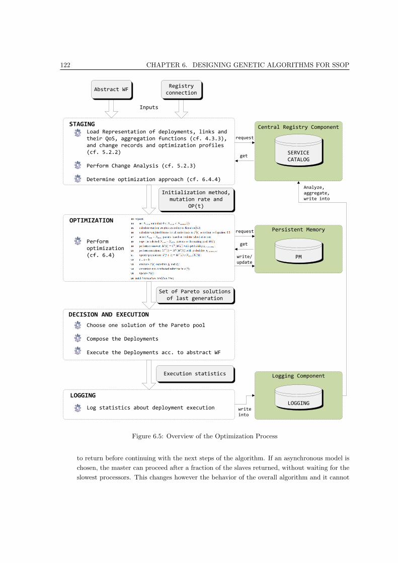
122 CHAPTER 6. DESIGNING GENETIC ALGORITHMS FOR SSOP
Inputs
Load Representation of deployments, links and their QoS, aggregation functions (cf. 4.3.3),and change records and optimization profiles (cf. 5.2.2)
Perform Change Analysis (cf. 5.2.3)
Determine optimization approach (cf. 6.4.4)
Abstract WFRegistry connection
Initialization method, mutation rate and
OP(t)
Perform optimization(cf. 6.4)
STAGING
OPTIMIZATION
Set of Pareto solutions of last generation
DECISION AND EXECUTION
Choose one solution of the Pareto pool
Compose the Deployments
Execute the Deployments acc. to abstract WF
LOGGING
Execution statistics Logging Component
LOGGINGLog statistics about deployment execution
request
get
Analyze, aggregate,write into
write into
Persistent Memory
PM
Central Registry Component
SERVICE CATALOG
request
get
write/update
Figure 6.5: Overview of the Optimization Process
to return before continuing with the next steps of the algorithm. If an asynchronous model is
chosen, the master can proceed after a fraction of the slaves returned, without waiting for the
slowest processors. This changes however the behavior of the overall algorithm and it cannot

6.4. AD-MOGA 123
safely be compared with its sequential equivalent. It has to be pointed out that the handling
of the master and slaves processes introduces a communication overhead. Therefore, such a
model is only profitable for problem settings with very complex fitness evaluation functions,
in which the gain from parallel processing by far outweighs the introduced communication.
2. Island models constitute a data decomposition approach [21], i.e., the algorithm is concurrently
evolved on different subsets of data. Typically, the population is divided into several subpop-
ulations (also called islands), each containing a subset of the individuals. The algorithm is
run on each island and each individual only competes with the other individuals belonging to
the same subpopulation [67]. In order to converge towards a global solution, individuals from
time to time have to be exchanged between subpopulations. For this process referred to as
migration [67], several parameters have to be introduced: the migration rate, migration inter-
val, migration scheme (defining which individuals are migrated: the best, the worst, random
ones, etc.) and the topology (defining if individuals can migrate to any other subpopulation
or only neighboring ones). Depending on the number of subpopulations and individuals per
subpopulation, coarse-grained (few subpopulations with many individuals) and fine-grained
(many subpopulations with few individuals) models are distinguished.
3. Hybrid methods combine ideas from the above-mentioned and other parallelization models.
For example, subpopulations can be overlapping. In this case, no migration is defined between
subpopulations, but individuals in overlapping regions can evolve in all of them. The spatial
structure then defines the interaction between individuals [67]. If there are many of those
overlapping subpopulations, each containing very few individuals, the algorithm is said to be
massively parallel [67]. The spatial structure in which the individuals are placed is commonly a
two-dimensional grid, but can also be a hypercube, for example. The ideal case is to assign one
individual to each processing element as disposal. This technique can be used on massively par-
allel computers for very large problem settings requiring complex computations. Furthermore,
subpopulations could be dynamic, self-adapting, etc., leading to new hybrid parallelization
methods.
All of the above mentioned methods come with costs, be they related to the communication be-
tween processes, or to the need for new parameters that have to be determined properly. Therefore,
the gain from parallelization in general and a specific method in particular, has to be evaluated
per algorithm and problem setting. Additionally, the choice is dependent on the available hard-
ware and computer architectures, because each method is best applied to a specific architecture.
For example, coarse-grained island models map well to a multiple-instruction, multiple data stream
(MIMD) model [2, 67]. Regarding the computational gain obtained with parallelization, Alba and
Tomassini [2] propose different definitions of speedup. They point out that a parallel GA has to be
compared with its exact sequential counterpart under identical conditions, which is not straightfor-
ward due to the stochastic nature of a GA. For example, the number of iterations studied in the
sequential and the parallel case cannot be fixed because it can lead to solutions of different quali-
ties. Rather, the stopping criterion of the parallel algorithm has to be such that the quality of the
solutions is identical to the ones obtained with the sequential algorithm. Most of the parallelization
methods will most likely not lead to a linear speedup function, but rather to a super-linear speedup

124 CHAPTER 6. DESIGNING GENETIC ALGORITHMS FOR SSOP
followed by a negative speedup for a number of processes higher than a certain threshold. This in
turn has to be determined per algorithm, platform, and problem setting.
Although a first and very basic approach for parallelizing a GA for the QoS-aware service selection
problem has been studied by the author and P.P. Beran in [13], it is argued that the rather small
problem settings encountered in realistic scenarios and the relatively inexpensive fitness functions do
not make parallelization a very promising direction. However, in the context of scalability studies,
in which AD-MOGA is applied to very large (simulated) problem spaces, parallelization can be a
future research direction.
6.5 Related Work
In this section, closely related work on applying multi-objective GAs to QoS-aware service selection
problems is surveyed. The main references and algorithms proposed are described, and the applied
concepts and methods are summarized in Tables 6.3 and 6.4. The algorithmic contribution of this
thesis presented in Section 6.4 builds on the knowledge gained from those related works, and extends
them as aforementioned.
Canfora et al. [22] seem to have been the first to propose the use of GAs for solving QoS-aware
service selection problems specifically. The authors define several QoS attributes and their aggrega-
tion functions, and a single-objective fitness function including costs, response time, availability and
reliability, and respective weights. They enable constraint handling by introducing a distance-based
penalty function reflecting the distance from constraint satisfaction. This distance measure is also
part of the fitness function, and its weight can either be static or dynamically increasing, in order to
allow potentially good solutions, but violating the constraints, in the early generations. The selec-
tion is based on roulette wheel, and crossover and mutation probabilities are fixed to 0.7 and 0.01
respectively. The elitist strategy used is to keep the two best individuals across generations. The au-
thors perform simulations and compare their approach to integer programming. They conclude that
their GA outperforms integer programming when the number of deployments per service exceeds
17, in their specific setup. For small systems, integer programming is the preferred approach.
Jaeger and Muhl [52] extend the work presented in [22]. They use the same QoS values and fitness
functions and analyze the impact of varying the mutation probability, the number of generations,
the structure of the fitness function and the penalty factor. Their simulations determine good values
or value ranges for these factors. These values are however specific to the exact implementation of
the algorithm. Additionally, they compare the GA to an exhaustive search, a branch-and-bound
and a local hill-climbing approach, in terms of the QoS value reached. While the exhaustive search
and the branch-and-bound algorithm do not perform in reasonable time in large problem settings,
they are used to determine the optimal QoS value. The GA proves to have a capability superior to
the hill-climbing, but it does not reach 50% of the optimal QoS value. This is a surprising result, as
also pointed out by the authors, but there is no further investigation.
Li et al. [60, 61] applied two existing GA, with small modifications, to the QoS-aware service
selection problem. In [60], the authors evaluate the application of the Strength Pareto Evolutionary
Algorithm 2 (SPEA2), presented in [110], to the service selection problem. They carry out a series
of simulations with 4 services having 90 to 500 deployments each. Results show that SPEA2 is able

6.5. RELATED WORK 125
to guide the search towards the Pareto front. The input parameters to the algorithm are provided,
but no explanation is given about how they have been determined. Additionally, questions about
specific behavior are left open, for example why the algorithm converges quicker when each service
has 500 deployments compared to 200. Only sequences of services are considered in this paper.
The SPEA2 algorithm is outlined in Algorithm 6 [110]. In [61] Li et al. apply the Nondominated
Sorting Genetic Algorithm II (NSGA-II) algorithm, proposed in [33], to the service selection problem.
Simulation runs for two different setups are carried out, one with 4 services having 90 deployments
each, the second one with 12 services having 30 deployments each. Results show that in both settings
the number of non-dominated solutions increases approximately at the same rate, suggesting that
NSGA-II distributes the solutions well on the Pareto front. The NSGA-II procedure is outlined in
Algorithm 7. The author’s plan is to compare SPEA2 and NSGA-II in QoS-aware service selection
environments in a future work project.
Earlier, Claro, Albers and Hao [29] suggested using NSGA-II for the same kind of problem. In
their simulations, they assessed the quality of the results as well as the scalability of the approach.
The authors show that feasible Pareto-optimal solutions are found, and an increasing number of
populations is needed with increasing problem setup, i.e., number of services and tasks.
Algorithm 6: SPEA2: Strength Pareto Evolutionary Approach 2
1 Pop: Population size;
2 N : Archive size;
3 maxGen: Maximal number of generations;
4 Initialize Population P (0);
5 Create empty Archive P (0);
6 t = 0;
7 repeat
8 Compute Fitness of Individuals in P (t) and P (t);
9 Copy all non-dominated solutions from P (t) and P (t) to P (t+ 1);
10 if size(P (t+ 1) ≥ N) then
11 reduce P (t+ 1) by specific truncation operator;
12 else
13 Fill P (t+ 1) with dominated solutions from P (t) and P (t)
14 end
15 Binary Tournament Selection to fill the Mating Pool;
16 Apply crossover and mutation;
17 t = t+ 1
18 until termination condition true;
Liu et al. [62] were among the first ones to suggest the use of a multi-objective GAs to solve the
service selection problem modeled as a multi-constraint multi-objective optimal path problem. Their
proposed algorithm, named Global Optimization of Dynamic Web Services Selection (GODSS), is
listed in Algorithm 8. The objectives, as described by the authors, are to minimize costs and
execution time of a workflow, while having constraints on reputation and reliability. No evaluation

126 CHAPTER 6. DESIGNING GENETIC ALGORITHMS FOR SSOP
Algorithm 7: NSGA-II: Non-Dominated Sorting Genetic Algorithm-II
1 create initial population;
2 repeat
3 fastNonDominatedSort;
4 crowdDistanceSort;
5 nonDominateSelect;
6 crossover;
7 mutate;
8 for i = 1 to popSize do
9 for j = 1 to NumOfObjectives do
10 computeFitness(i,j);
11 end
12 end
13 until termination condition true;
of the algorithm is carried out.
Algorithm 8: Global Optimization of Dynamic Web Services Selection (GODSS)
1 Produce a set of initial feasible composition paths.;
2 Produce initial population (fixed-length-integral coding);
3 repeat
4 Fitness Assignment (Pareto-based) and maintenance of diversity (based on entropy theory);
5 Elitism (keep non-dominated solutions);
6 Selection (Roulette Wheel);
7 Crossover;
8 Mutation;
9 Yield new population;
10 until termination condition true;
11 Output: set of Pareto-optimal composition paths;
An interesting approach for addressing the QoS optimization of Grid workflows is presented by
Tong, Cao and Zhang [80]. Starting from the observation that a Grid environment is composed
of independent domains, they propose a distributed GA, where the population is divided into sub-
populations, and each subpopulation is evolved at a domain. According to predefined migration
interval and rate, individuals from the Pareto set of each subpopulation are migrated to a neigh-
boring subpopulation, replacing the worst two individuals there. This communication mechanism
between subpopulations can be considered as an implicit elitism. This distributed GA, outlined in
Algorithm 9, can easily be parallelized, which allows reducing its overall computation time. Exper-
iments have been conducted in a setup involving 16 abstract services having 32 deployments each,
10 domains (subpopulations) and 50 individuals per subpopulation. The objectives are to minimize
overall costs and execution time, while meeting constraints imposed on reliability, reputation and

6.5. RELATED WORK 127
security. Results show that the Pareto set converges after about 100 generations, and that the two
objectives are really independent. No conclusions regarding the computation time and no compar-
isons to other approaches are made. The authors point out that in their paper the QoS values are
assumed static, and future work would involve considering dynamics inherent in a Grid environment.
However, surveying the existing literature, it seems that no such work has been presented yet.
Algorithm 9: Distributed Multi-Objective Genetic Algorithm by Tong et al. [80]
1 Generate initial population randomly;
2 Divide the initial population into n subpopulations;
3 Evaluate the individuals according to fitness function;
4 repeat
5 Binary tournament selection ;
6 Crossover and Mutation;
7 Evaluate the individuals according to fitness function;
8 if Migration condition then
9 Perform migration and evaluation
10 end
11 until termination condition true;
The work of Wada et al. [90, 92] is close to the approach presented in this thesis. In [90], the
authors introduce E3-MOGA, a multi-objective genetic algorithm that considers multiple service
level agreements (based on QoS) simultaneously and optimizes service compositions. It outputs a
set of Pareto-optimal solutions as trade-off, and the final decision is up to the user. The considered
QoS attributes are throughput, latency and cost, and overall qualities are defined at three levels,
platinum, gold and silver. The authors start from the assumption that probability distributions of
QoS measures can be determined based on the analysis of historical data. They conducted simula-
tions with four abstract services having three deployments each, at different QoS levels, showing the
applicability of E3-MOGA. Recently, the authors extended their work in several ways to address
deployment optimization in cloud computing environments [92]. Here, queuing theory is leveraged
to predict the throughput and latency of atomic and composite services. Additionally, the authors
propose an objective reduction mechanism that allows identifying redundant objectives and thus
reduce the number of them. Indeed, in optimization problems with more than three objectives,
solutions tend to be non-dominated, i.e., it is rare to find solutions that are better than others re-
garding all objectives. The presented overall optimization algorithm is referred to as E3-R. Is is built
on E3-MOGA as described above, leveraged by mechanisms to predict deployment performance and
to reduce the number of objectives.
Wang and Hou [93] present a QoS-aware service selection problem taking into account three
objectives (minimization of the costs, minimization of the response time and maximization the reli-
ability), three control structures (sequence, parallel, choice), and inter-services constraints (alliance,
competition or no relation between services). They use a binary encoding and propose a multi-
objective GA with selection based on Pareto ranking, one-point crossover and elitism. Experiments
conducted with a total of 35, 70 and 105 deployments in total show that the algorithm reaches 91%

128 CHAPTER 6. DESIGNING GENETIC ALGORITHMS FOR SSOP
of the optimal values for all three QoS measures.
The methods employed in AD-MOGA and in the related work described in this section are
summarized in Tables 6.3 and 6.4. It can be seen that none of the closely related work is considering
the dynamic aspects of the underlying system. This thus constitutes a contribution of this thesis.
6.6 Summary
Genetic algorithms can be used to solve both single- and multi-objective QoS-aware service selection
problems. When designing multi-objective GA, specific design considerations have to be taken into
account, mostly in order to ensure that diversity of the population is kept across generations and
thus prevent the algorithm from converging towards a local optimum. In the literature, several works
are found that deal with the direct application of multi-objective GAs to QoS-aware service selection
problems. However, none of the presented GA-based approaches allows the representation of general
flow structures, and the explicit consideration of dynamics encountered in the underlying system
made up of services, resources and deployments. To bridge this gap, an adaptive and dynamic multi-
objective GA, referred to as AD-MOGA, has been introduced in this chapter. It allows taking into
account optimization profiles (as defined in Chapter 5) through the use of random weights assigned
within predefined ranges. These random weights also ensure that diversity is kept in the population
of the GA. It further makes use of an explicit, persistent storage of good solutions from previous
optimization runs to ensure a good initial population, and implements an adaptive mutation rate
depending on the impact of system changes. The next chapter presents the evaluation results of this
approach.

6.6. SUMMARY 129
Ref
eren
ceE
nco
din
gO
per
ator
sF
itn
ess
Div
ersi
tyE
liti
smC
on
stra
ints
Dyn
am
ics
[22,
52]
Inte
ger
2-p
oints
cros
sover
,
Rou
lett
e
wh
eel
sele
c-
tion
Sin
gle
-
ob
ject
ive
n/a
Yes
Dis
tan
ce-
base
d
pen
alt
y
No
[60,
110]
Inte
ger
1-p
oint
cros
sover
,
Bin
ary
tou
r-
nam
ent
sele
ctio
n
Pare
to-
dom
inan
ce
an
dd
ensi
ty
Fit
nes
ssh
ar-
ing
Yes
,in
extr
a
list
n/a
No
[61,
29]
Inte
ger
Bin
ary
tou
r-
nam
ent
sele
ctio
n
Non
-
dom
inate
d
sort
ing
Cro
wd
ing
dis
tan
ce
Yes
Pen
alt
y
fun
ctio
n
No
[62]
Inte
ger
(fixed
-
len
gth
)
2-p
oints
cros
sover
,
Rou
lett
e
wh
eel
sele
c-
tion
Pare
toso
rtIn
form
ati
on
entr
opy
Yes
Dea
th
pen
alt
y
No
Tab
le6.
3:C
omp
aris
onof
Ap
pro
ach
esto
QoS
-Aw
are
Ser
vic
eS
elec
tion
wit
hG
A(1
)

130 CHAPTER 6. DESIGNING GENETIC ALGORITHMS FOR SSOP
Ref
eren
ceE
nco
din
gO
per
ator
sF
itn
ess
Div
ersi
tyE
liti
smC
on
stra
ints
Dyn
am
ics
[80]
Inte
ger
Cro
ssov
er
not
imp
le-
men
ted
,
Bin
ary
tou
r-
nam
ent
sele
ctio
n
Dom
inati
on
ran
k
n/a
n/a
Pen
alt
y
fun
ctio
n
No
[90]
Inte
ger
(fixed
-len
gth
arra
y)
Rou
lett
e
wh
eel
sele
c-
tion
Dom
inati
on
ran
kan
d
den
sity
Cel
l-b
ase
d
den
sity
Yes
Pen
alt
y
fun
ctio
n
No
[93]
Bin
ary
stri
ng
1-p
oint
cros
sover
Pare
to-
ran
kin
g
No
Yes
,in
-
sid
eth
e
pop
ula
tion
No
No
AD
-MO
GA
(th
isth
esis
)
Sp
ecia
lre
fer-
ence
enco
d-
ing
(cf.
6.4.
1)
1-p
oint
cros
sover
,
Rou
lett
e
wh
eel
sele
c-
tion
Pare
to-
base
d,
ran
dom
wei
ghts
Ran
dom
wei
ghts
Yes
,in
-
sid
eth
e
pop
ula
tion
Dea
th
pen
alt
y
Yes
Tab
le6.
4:C
omp
aris
onof
Ap
pro
ach
esto
QoS
-Aw
are
Ser
vic
eS
elec
tion
wit
hG
A(2
)

Chapter 7
Implementation and Evaluation
This chapter presents and discusses the evaluation results of the optimization approach proposed in
Chapter 6. The evaluation of AD-MOGA focuses on three quantitative aspects. First, the “base”
multi-objective GA underlying AD-MOGA is evaluated regarding its convergence, its approximation
of the Pareto front and its diversity preservation. The “ideal” input parameters such as the mutation
and cross-over rate are also investigated. Second, the behavior of AD-MOGA is simulated in a
dynamic environment and its adaptability to changes is evaluated. Third, the algorithm is run
on increasing problem spaces, with the aim of evaluating its runtime performance and scalability.
Furthermore, a qualitative assessment is carried out. In particular, the integration of AD-MOGA
into the TAG system is shortly discussed. In fact, most of the steps described throughout this thesis
have been applied to the concrete TAG system. Therefore, experience could be gained regarding
the design, implementation and integration of a deployment selection optimization framework into
a real system. Especially when started from scratch, it is a long process that allows gaining deeper
understanding of the underlying distributed system, beyond the initial scope, but also has drawbacks
on the way.
This chapter is organized into sections as follows. Section 7.1 details the environment and setup
used for simulation and evaluation of the proposed GA. Section 7.2 discusses the general applicability
of AD-MOGA to service selection problems, and shows to what extent the algorithm approximates
the Pareto front. In Section 7.3 the results of the evaluation of AD-MOGA regarding accuracy,
stability and reaction capability are presented and discussed. The evaluation results of the runtime
performance as well as the scalability of AD-MOGA with increasing problem spaces are presented
in Section 7.4. The subsequent two sections specifically deal with the TAG system. Section 7.5
discusses the integration of AD-MOGA into the deployment selection optimization inside the TAG
system. In Section 7.6 the experience gained while implementing a deployment selection optimization
framework in a concrete distributed system is reflected, outlining the gains in terms of reached goals,
as well as the drawbacks. Section 7.7 highlights possible enhancements and extensions for future
work. Finally, the chapter is summarized in Section 7.8.
131

132 CHAPTER 7. IMPLEMENTATION AND EVALUATION
7.1 Simulation and Evaluation Setup
Although the approach is motivated by a real-world application, a simulation and evaluation environ-
ment has been set up. The reasons for this are manifold. First, simulation runs are computationally
expensive and should not be carried out on a real-world production system. Second, the approach is
evaluated on different setups, with different data constellations, etc. which cannot be realized on the
fly on a production system. Finally, for studying the scalability of the approach, the problem space
has to be bigger than the current TAG production system. Therefore, a simple registry has been
created on a separate database schema. The data model is depicted in Figure 7.1. It is simpler than
the TASK service catalog presented in Chapter 4, but holds the key concepts needed for carrying
out the deployment selection, namely services, deployments, links and related attributes such as
performance and usage indexes as well as other QoS metrics.
Attribute
PK AID
FK1 Name
DhasAttribute
PK,FK2 DIDPK,FK1 AID
Value
Deployment
PK DID
NameFK1 SID
Link
PK LID
FK1 OriginDIDFK2 DestDID
Service
PK SID
Name
LhasAttribute
PK,FK2 LIDPK,FK1 AID
Value
Figure 7.1: Simulation Setup: Database Schema
The tables are deployed on a development Oracle database hosted at CERN. AD-MOGA is
implemented in Python and interacting with the database through SQLAlchemy [64], a Python
SQL toolkit and object-relational mapper. The implemented classes are as shown in Figure 7.2. The
class System captures the environment, that is the available system components and their attributes.
These are loaded from the database via the utils package that uses the class DBConnectionHandling
to interact with the central QoS repository. The components and their associated attributes are
internally represented in Python dictionaries and queried throughout the optimization process. An
instance of the class GeneticAlgorithm is created to start the optimization. It implements all the
methods needed to evolve the population, such as getFitness(), mutate() and crossover().
The algorithm is run locally. In order to be able to start simulation runs online and make use
of a Cloud infrastructure, a related deployment selection simulation tool has been implemented on
the Google App Engine [43]. The main goal of this joint work [13] with P. P. Beran (cf. Chapter 1,
Section 1.4) was to compare a GA with a Blackboard approach on a common simulated problem
setup. While the implementation of the optimization framework was straightforward and the com-

7.1. EVALUATION SCENARIO I 133
parison worked well for small problem settings, as expected it turned out not to be scalable for
bigger simulation runs. This implementation thus had been considered as a proof of concept and
has not been further investigated, nor used for the evaluation described in this chapter.
For carrying out the simulation runs, problem settings of different sizes have been created. The
database schema presented above is populated using SQL and Python scripts, to which the total
number of services and the number of deployments for each service are provided as input. Attribute
values are randomly generated within predefined ranges. All simulation runs are based on at least
20 distinct experiments independent of each other.
+__init__()
+print_system()
System
+engine
+services
+deployments_dict
+deployments_qos_dict
+deployments_links_dict
+optimization_profile
+__init__()
+initializeRandomPopulation()
+initialPopulationFromMemory()
+crossover()
+mutate()
+getFitness()
+getWeightedFitness()
+getParetoSolutions()
+getDominatedSolutions()
+getLinks()
+iPopSize
+iGenerations
+fCrossRate
+fMutationRate
GeneticAlgorithm
+connect()
+disconnect()
+engine
DBConnectionHandling
utils1
+uses
1
*
+uses
1
*
+uses1
+runs_on
*
+defines_scope
*
Figure 7.2: Classes and Packages in the Prototype Implementation
7.2 Evaluation Scenario I: Applicability of AD-MOGA, Pareto
Approximation and Input Parameters
The first series of simulation runs aims at evaluating the ability of AD-MOGA to approximate the
Pareto front (cf. Chapter 5, Section 5.4.2). For small problem setups, an exhaustive search algorithm
has been run to determine the real Pareto solutions, and it has been verified that the solutions found
with AD-MOGA are identical to those of the exhaustive search, and thus that AD-MOGA reaches
the Pareto front. For bigger problem setups however, the exhaustive search could not be run on
custom hardware, due to a lack of memory. It cannot be assumed that AD-MOGA reaches the
Pareto front for large setups, but since its principal convergence has been demonstrated, it can be
assumed that it approximates the Pareto front. The results of AD-MOGA, after a certain number
of generations, are thus referred to as Pareto candidates. The test runs have been configured such

134 CHAPTER 7. IMPLEMENTATION AND EVALUATION
that the Pareto candidates are also logged for a high number of generations, e.g., 500. It cannot be
guaranteed that the result after 500 generations is the real Pareto front, but it can be considered as
a fair approximation.
The first simulation runs have also been used as “calibration” regarding the input parameters,
namely the population size, and the crossover and mutation rates. The following parameters lead
to the most promising results:
• Population size: 100
• Crossover rate: 0.65
• Mutation rate: 0.02
However, it has to be pointed out that the optimal size of the population is dependent on the
problem size. For small setups e.g., with 5 to 10 services having on average 5 deployments each (i.e.,
a realistic size of the TAG application system), a population comprising 50 individuals is big enough
to show a good convergence towards the Pareto front at generation 100. But for these first test
series the population size has been fixed at 100 in order to maintain the same parameters through
the 6 runs.
The following simulation runs have been carried out with an even deployment distribution:
• Run 1: 5 services, 5 deployments each, workflow of 5 services, no constraints.
• Run 2: 5 services, 20 deployments each, workflow of 5 services, no constraints.
• Run 3: 10 services, 5 deployments each, workflow of 10 services, no constraints.
• Run 4: 10 services, 20 deployments each, workflow of 10 services, no constraints.
• Run 5: 20 services, 5 deployments each, workflow of 20 services, no constraints.
• Run 6: 20 services, 20 deployments each, workflow of 20 services, no constraints.
The following simulation runs have been carried out with an uneven deployment distribution (i.e.,
the services have different numbers of deployments):
• Run 1: 5 services, 100 deployments total (5-10-20-30-35), workflow of 5 services, no constraints.
• Run 2: 5 services, 100 deployments total (35-30-20-10-5), workflow of 5 services, no constraints.
• Run 3: 10 services, 200 deployments total (2-5-10-15-18-20-25-30-35-40), workflow of 10 ser-
vices, no constraints.
• Run 4: 10 services, 200 deployments total (40-35-30-25-20-18-15-10-5-2), workflow of 10 ser-
vices, no constraints.
• Run 5: 20 services, 400 deployments total (2-2-5-5-10-10-15-15-18-18-20-20-25-25-30-30-35-35-
40-40), workflow of 20 services, no constraints.
• Run 6: 20 services, 400 deployments total (40-40-35-35-30-30-25-25-20-20-18-18-15-15-10-10-
5-5-2-2), workflow of 20 services, no constraints.

7.2. EVALUATION SCENARIO I 135
Abstract workflows composed of 5 to 10 distinct services represent a reasonable scenario in real-
world applications. Workflows containing 20 or more services, and each service having multiple
deployments, are scenarios that can be used to test the scalability of an approach, but they are
most likely not representative of concrete applications. In the TAG use case for example, there exist
about 10 distinct services, and typical workflows do not involve all of them.
Figure 7.3 shows the results for the 6 simulation runs with even deployment distribution described
above. Each plot represents the non-dominated solutions at different generations, namely generation
0 (random initialization), and the generations 20, 40, 60, 100, 300 and 500. Figure 7.4 shows the
respective results for the 6 runs with uneven deployment distribution.
35
40
45
50
55
60
65
70
75
10 12 14 16 18 20 22 24 26 28 30 32
Per
form
ance
Inde
x
Usage Index
Pareto Approximation (Even) - Run 1
g0g20g40g60
g100g300g500
3540455055606570758085
8 10 12 14 16 18 20 22 24 26
Per
form
ance
Inde
x
Usage Index
Pareto Approximation (Even) - Run 2
g0g20g40g60
g100g300g500
80
90
100
110
120
130
140
150
160
25 30 35 40 45 50 55 60 65
Per
form
ance
Inde
x
Usage Index
Pareto Approximation (Even) - Run 3
g0g20g40g60
g100g300g500
708090
100110120130140150160170
15 20 25 30 35 40 45 50 55
Per
form
ance
Inde
x
Usage Index
Pareto Approximation (Even) - Run 4
g0g20g40g60
g100g300g500
200210220230240250260270280290300310
40 50 60 70 80 90 100 110
Per
form
ance
Inde
x
Usage Index
Pareto Approximation (Even) - Run 5
g0g20g40g60
g100g300g500
200
220
240
260
280
300
320
340
30 40 50 60 70 80 90 100 110
Per
form
ance
Inde
x
Usage Index
Pareto Approximation (Even) - Run 6
g0g20g40g60
g100g300g500
Figure 7.3: Approximation of the Pareto Front: Even Deployment Distribution
Figure 7.3 shows that for small system setups (Runs 1 to 3), AD-MOGA is converging after
about 60 generations. For bigger setups (Runs 4 to 6), there are still small improvements between
generation 300 and 500, but the Pareto candidates at generation 100 can be considered as a good
approximation. It can also be seen that the algorithm makes a good approximation of the entire

136 CHAPTER 7. IMPLEMENTATION AND EVALUATION
45
50
55
60
65
70
75
80
85
10 15 20 25 30 35 40
Per
form
ance
Inde
x
Usage Index
Pareto Approximation (Uneven) - Run 1
g0g20g40g60
g100g300g500
40
45
50
55
60
65
70
75
80
8 10 12 14 16 18 20 22 24 26 28
Per
form
ance
Inde
x
Usage Index
Pareto Approximation (Uneven) - Run 2
g0g20g40g60
g100g300g500
100
110
120
130
140
150
160
170
20 25 30 35 40 45 50 55
Per
form
ance
Inde
x
Usage Index
Pareto Approximation (Uneven) - Run 3
g0g20g40g60
g100g300g500
100105110115120125130135140145150155
15 20 25 30 35 40 45 50 55 60 65 70
Per
form
ance
Inde
x
Usage Index
Pareto Approximation (Uneven) - Run 4
g0g20g40g60
g100g300g500
200
220
240
260
280
300
320
340
60 70 80 90 100 110 120 130
Per
form
ance
Inde
x
Usage Index
Pareto Approximation (Uneven) - Run 5
g0g20g40g60
g100g300g500
180
200
220
240
260
280
300
320
50 60 70 80 90 100 110 120 130 140
Per
form
ance
Inde
x
Usage Index
Pareto Approximation (Uneven) - Run 6
g0g20g40g60
g100g300g500
Figure 7.4: Approximation of the Pareto Front: Uneven Deployment Distribution

7.2. EVALUATION SCENARIO II 137
front, i.e., no genetic drift can be observed. Comparing Figure 7.3 and Figure 7.4, it can be noticed
that in general the approximation converges faster for even deployment distributions. In rather
“random” distribution scenarios, more generations are required to reach the Pareto front. This thus
has to be considered when setting up the input parameters for the algorithm.
7.3 Evaluation Scenario II: Adaptability to Changes
7.3.1 Formal Evaluation Criteria for Dynamic GA
Evaluating the performance of an adaptive GA in a dynamic environment is more complex than
evaluating a GA in a static environment, and special techniques are required. Weicker [96] sum-
marizes three important measures in dynamic optimization: optimization accuracy, stability and
reactivity. The optimization accuracy defines the quality of the best individual at time t compared
to the overall best quality at time t. For the multi-objective case, this can either be computed
by assigning weights to the objectives, thus reducing the problem to a single-objective one, or by
calculating an average of the Pareto approximation. It is the same measure as the one evaluated in
Section 7.2, with the difference that it is defined for a specific time t only. According to Weicker [96],
an adaptive algorithm is called stable “if changes in the environment do not affect the optimization
accuracy severely. That means that a stable, adaptive algorithm is required to be prepared for
changes in the environment”. The related metric is referred to as stability. Finally, the reactivity
can be considered as a combination of accuracy and stability. It refers to the time needed to adapt
to a change in the underlying environment. When evaluating a GA, this time can be measured in
number of generations.
In the following subsections, these performance metrics are investigated for AD-MOGA, with
the types of changes described in Chapter 6 (Section 6.4.4).
7.3.2 Implementation of the Persistent Memory
The “persistent memory” in which good individuals from past optimization runs are stored is in-
tegrated into the central QoS registry. As depicted in Figure 6.4 it is composed of a simple table
that references the table storing the optimization profile. The granularity of the table is defined by
the pair composed of the optimization profile ID (OP ID) and the abstract workflow (abstract WF).
That is, for each such combination the latest generation or latest Pareto set of the last optimization
run is stored, and a timestamp indicates the insert or update date of the entry. Figure 7.5 shows the
sequence of actions when the memory is queried. First, the timestamp of the related memory entry
is compared with all timestamps indicating system changes. When changes have occurred, they are
first evaluated (i.e., the similarity index is computed) and then, based on the result of this index,
the memory entry is retrieved or not. The update mechanism is similar. Each optimization run
updates its corresponding memory entry, identified again by the (OP ID, abstract WF) pair. Or, if
such an entry does not yet exist, it is inserted.

138 CHAPTER 7. IMPLEMENTATION AND EVALUATION
changeHandler changeEvaluator centralRegistry
requestChanges
returnChanges
evaluateChanges
postSimilarityIndex
requestLastPopulation
returnPartialPopulation
Analysis of change timestamps
Cf. Section 5.2.3
SELECT last_generation
FROM MemoryGASolutions
WHERE OP_ID = <input>
AND abstract_wf = <input>
Partial old population to be inserted
into new initial population.
Figure 7.5: Schematic Query of the Persistent Memory
7.3.3 Changes During or Between Optimization Runs
In these test series, AD-MOGA is evaluated under the change conditions described in Table 6.2.
(The scenario numbers also refer to those defined in Table 6.2.)
Scenario (4): ((WF,OP (t)) in PM , and no system change. The pair composed of the abstract
input workflow and the optimization profile exists in the persistent memory, and no change has
happened since the last execution. In this case, no optimization has to be done because the
previous solution can simply be reused. Therefore, the Pareto candidates stored in the PM
are retrieved and passed on to the Decision and Execution stage of the optimization approach
(cf. Figure 6.5).
Scenarios (1), (2) and (5): ((WF,OP (t)) in PM , and non-radical system changes. To eval-
uate these scenarios, the following setup and steps are considered:
• System composed of 10 services having 5 deployments each (because this setup is closest
to the reality of the TAG application scenario).
• Sequential workflow composed of 10 distinct abstract services.
• At time t, the system has a certain status: SP (t) and OP (t) as described in Chapter 5,
Section 5.2. The GA is started for an abstract workflow W0 and the Pareto candidates
are evaluated as shown in Run 1 of Figure 7.6.

7.3. EVALUATION SCENARIO II 139
• At time t + ∆t, there is a new request with the same workflow W0 as input. Between t
and t+ ∆t, the attribute value levels of two deployments of service 1, one deployment of
service 2 and one deployment of service 3 have changed, as defined in Section 5.2. In a
sequence of 10 deployments, there are 9 links, thus 19 components in total. According to
Equations 5.6 to 5.9, and defining the three changed deployments as D1(S1), D2(S2) and
D3(S3), this results in the following similarity index :
impCi=
1
19(7.1)
siD1(S1) =1
19·(
1− 2
5
)siD2(S2) =
1
19·(
1− 1
5
)siD3(S3) =
1
19·(
1− 1
5
)siDi
=1
19, for i = 4, ..., 10
siL =1
19· (9− 0) =
9
19
sitotal =
10∑i=4
·siDi+ siD1(S1) + siD2(S2) + siD3(S3) + siL =
91
95' 0.958
Therefore, overall the system is qualified as having “slightly changed” (cf. Figure 5.1).
• According to Table 6.2, the population is thus initialized with a fraction of the best
individuals computed at time t, and the mutation rate is increased.
The plot for Run 2 in Figure 7.6 shows the convergence achieved using this technique. Con-
cretely, the 18 individuals from the Pareto candidates computed in the previous optimization
at time t have been inserted into the initial population, and the remaining 82 individuals have
been initialized randomly. The mutation rate has been raised from 0.02 to 0.04. It can be
seen that the algorithm converges rapidly without however losing its diversity range. As a
comparison, Run 3 in Figure 7.6 depicts the convergence using a random initial population,
similar to the one of Run 1. It can be concluded that in such a case the number of total
generations can be reduced, thus reducing the total runtime of the algorithm. Alternatively,
if another termination criterion is used (e.g., the number of new/changes Pareto candidates
between generations), the algorithm will simply stop earlier.
Figure 7.7 shows the results for a similar test series as described above, but with more important
changes between the optimization runs. Concretely, in this scenario changes were recorded on
10% of the components (deployments and links).
Figure 7.8 shows the results of a repeated similar test, but with a change rate of 50% (the
change rate corresponds to one minus the similarity index). In this case, it can be seen that
a restart with memory and a mutation rate of 0.05 present no advantage over a random
initialization. Raising the mutation rate to 0.1 shows better results, which suggests that a
gradual adaptation of the mutation rate as a function of the system change rate is a valid
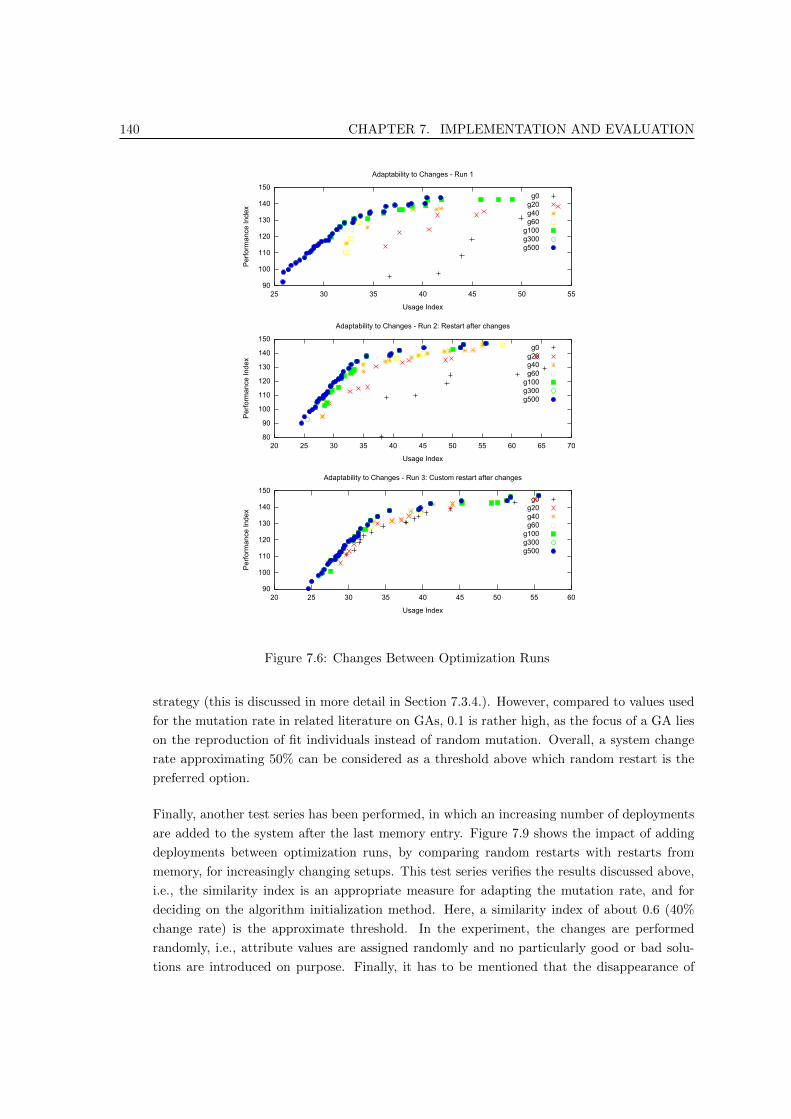
140 CHAPTER 7. IMPLEMENTATION AND EVALUATION
90
100
110
120
130
140
150
25 30 35 40 45 50 55
Per
form
ance
Inde
x
Usage Index
Adaptability to Changes - Run 1
g0g20g40g60
g100g300g500
80
90
100
110
120
130
140
150
20 25 30 35 40 45 50 55 60 65 70
Per
form
ance
Inde
x
Usage Index
Adaptability to Changes - Run 2: Restart after changes
g0g20g40g60
g100g300g500
90
100
110
120
130
140
150
20 25 30 35 40 45 50 55 60
Per
form
ance
Inde
x
Usage Index
Adaptability to Changes - Run 3: Custom restart after changes
g0g20g40g60
g100g300g500
Figure 7.6: Changes Between Optimization Runs
strategy (this is discussed in more detail in Section 7.3.4.). However, compared to values used
for the mutation rate in related literature on GAs, 0.1 is rather high, as the focus of a GA lies
on the reproduction of fit individuals instead of random mutation. Overall, a system change
rate approximating 50% can be considered as a threshold above which random restart is the
preferred option.
Finally, another test series has been performed, in which an increasing number of deployments
are added to the system after the last memory entry. Figure 7.9 shows the impact of adding
deployments between optimization runs, by comparing random restarts with restarts from
memory, for increasingly changing setups. This test series verifies the results discussed above,
i.e., the similarity index is an appropriate measure for adapting the mutation rate, and for
deciding on the algorithm initialization method. Here, a similarity index of about 0.6 (40%
change rate) is the approximate threshold. In the experiment, the changes are performed
randomly, i.e., attribute values are assigned randomly and no particularly good or bad solu-
tions are introduced on purpose. Finally, it has to be mentioned that the disappearance of

7.3. EVALUATION SCENARIO II 141
80
90
100
110
120
130
140
150
25 30 35 40 45 50 55 60
Per
form
ance
Inde
x
Usage Index
10% Change Rate - Random Restart (Mutation: 0.02)
g0g20g40g60
g100g300g500
80
90
100
110
120
130
140
150
25 30 35 40 45 50 55 60
Per
form
ance
Inde
x
Usage Index
10% Change Rate - Restart with Memory (Mutation: 0.05)
g0g20g40g60
g100g300g500
Figure 7.7: 10% Change Rate Between Optimization Runs

142 CHAPTER 7. IMPLEMENTATION AND EVALUATION
115
120
125
130
135
140
145
150
155
25 30 35 40 45 50 55
Per
form
ance
Inde
x
Usage Index
50% Change Rate - Random Restart (Mutation: 0.02)
g0g20g40g60
g100g300g500
100105110115120125130135140145150
22 24 26 28 30 32 34 36 38 40 42 44
Per
form
ance
Inde
x
Usage Index
50% Change Rate - Restart with Memory (Mutation: 0.05)
g0g20g40g60
g100g300g500
100105110115120125130135140145150
20 25 30 35 40 45 50 55
Per
form
ance
Inde
x
Usage Index
50% Change Rate - Restart with Memory (Mutation: 0.1)
g0g20g40g60
g100g300g500
Figure 7.8: 50% Change Rate Between Optimization Runs
7.3. EVALUATION SCENARIO II 143
deployments has to be handled differently, as it invalidates previous solutions containing those
deployments.
Scenario (3): Change in OP (t). In this case, there is a change in the optimization profile during
a run, i.e., the weights of the optimization objectives change, or constraints are introduced. In
case a change in the weights is detected, several actions are taken: first, the fitness weighting
is adjusted, second, if the new (WF,OP (t)) pair exists in memory, a fraction of the current
population is replaced by individuals from memory, and the mutation rate is updated ac-
cordingly. Such changes are only assumed in long or continuously running optimizations. In
case constraints are introduced, the constraint handling procedure is enabled from the current
generation on.
Scenario (6): ((WF,OP (t)) in PM , and radical change) OR (((WF,OP (t)) not yet in PM).
In this scenario, either the pair consisting of the abstract input workflow and the optimization
profile does not yet exist in PM , or it does but a change categorized as radical has occurred
since the latest related memory record. In such a case, the algorithm has to be restarted and
the evaluation results presented in Section 7.2 are relevant.
In general, considering changes occurring during an optimization run is only sensible in case
of a continuous optimization process. In this case, a separate process regularly queries the central
registry to detect changes and signal them to the optimization process that then adapts to them,
according to the change rate.
7.3.4 Stepwise Adaptation of the Mutation Rate
As suggested in Figure 7.8, it seems beneficial to adapt the mutation rate to the change rate. A few
test series have been carried out to verify this assumption. An initial system comprising 10 services
having 5 deployments each has been set up, an optimization run has been carried out and the Pareto
solutions of the last generation have been saved into the persistent memory. Then, the system has
been changed randomly in three subsequent steps, so that the optimization could be run on setups
with decreasing similarity index, concretely 0.9, 0.8 and 0.7. For each of those changed setups,
optimizations with increasing mutation rates have been run. Considered rates are 0.02 (and random
restart), 0.03, 0.035 and 0.04 (restart from memory). The mutation rate is especially important in
order to ensure diversity in the population after a change. The results are shown in Figures 7.10, 7.11
and 7.12.
For a similarity index of 0.9, the best results are achieved with the lowest mutation rate tested,
namely 0.03. Augmenting the rate does not add diversity, nor lead to faster convergence – on
the contrary, the convergence seems to be degrading for a higher mutation rate. For the next lower
similarity index, 0.8, mutation rates of 0.03, 0.035 and 0.04 are almost equally good, no degradation is
observed for a rate of 0.04. Finally, for the lowest tested similarity index, 0.7, the earliest convergence
is achieved with the highest mutation rate, 0.04.
Adapting the mutation rate as a function of the similarity index thus seems to be a promising
strategy. However, in order to derive a possible relation factor, many more experiments in varying
system setups need to be performed. Additionally, a more fine-grained “zooming” into the population

144 CHAPTER 7. IMPLEMENTATION AND EVALUATION
100
110
120
130
140
150
20 25 30 35 40 45 50
Per
form
ance
Inde
x
Usage Index
4% Changes - Random Restart
g0g20g40g60
g100g300g500
90
100
110
120
130
140
150
20 25 30 35 40 45 50
Per
form
ance
Inde
xUsage Index
4% Changes - Restart with Memory (Mutation: 0.03)
g0g20g40g60
g100g300g500
90
100
110
120
130
140
150
20 25 30 35 40 45 50 55
Per
form
ance
Inde
x
Usage Index
10% Changes - Random Restart
g0g20g40g60
g100g300g500
90
100
110
120
130
140
150
20 25 30 35 40 45 50
Per
form
ance
Inde
x
Usage Index
10% Changes - Restart with Memory (Mutation: 0.035)
g0g20g40g60
g100g300g500
100
110
120
130
140
150
20 25 30 35 40 45 50
Per
form
ance
Inde
x
Usage Index
20% Changes - Random Restart
g0g20g40g60
g100g300g500
90
100
110
120
130
140
150
15 20 25 30 35 40 45 50
Per
form
ance
Inde
x
Usage Index
20% Changes - Restart with Memory (Mutation: 0.04)
g0g20g40g60
g100g300g500
100
110
120
130
140
150
160
15 20 25 30 35 40 45 50
Per
form
ance
Inde
x
Usage Index
40% Changes - Random Restart
g0g20g40g60
g100g300g500
90100110120130140150160
15 20 25 30 35 40 45 50
Per
form
ance
Inde
x
Usage Index
40% Changes - Restart with Memory (Mutation: 0.06)
g0g20g40g60
g100g300g500
Figure 7.9: Impact of Adding Deployments with Different Change Rates

7.3. EVALUATION SCENARIO III 145
evolution needs to be carried out. A detailed analysis in this area represents a possible direction for
future work.
100
105
110
115
120
125
130
135
140
145
150
25 30 35 40 45 50
Per
form
ance
Inde
x
Usage Index
Similarity: 0.9; Mutation: 0.02; Random Restart
g0g10g20g25g30
g100115
120
125
130
135
140
145
150
20 22 24 26 28 30 32 34 36
Per
form
ance
Inde
x
Usage Index
Similarity: 0.9; Mutation: 0.03; Memory Restart
g0g10g20g25g30
g100
110
115
120
125
130
135
140
145
150
155
20 22 24 26 28 30 32 34 36
Per
form
ance
Inde
x
Usage Index
Similarity: 0.9; Mutation: 0.035; Memory Restart
g0g10g20g25g30
g100115
120
125
130
135
140
145
150
155
20 22 24 26 28 30 32 34 36 38
Per
form
ance
Inde
x
Usage Index
Similarity: 0.9; Mutation: 0.04; Memory Restart
g0g10g20g25g30
g100
Figure 7.10: Impact of Varying Mutation Rates, Similarity Index 0.9
7.4 Evaluation Scenario III: Runtime Performance and Scal-
ability
For the algorithm to be applied to a real system, it has to be tested in terms of runtime performance
and scalability. In fact, if the time spent on the optimization is longer than the worst case execution
time when a random or hard-coded composition is chosen, the approach is useless in a real environ-
ment. As suggested by the tests shown in Figure 2.7 (Chapter 2), in the concrete TAG system there
is a rather large margin between the best and the worst combination – in this example timings are
done for the composition of only two deployments, and it can be assumed that this margin increases
with the length of the workflow. However, although this is not the primary focus in this evaluation,
much consideration has to be put on the optimization of the algorithm itself, in terms of runtime.
In order to do so, two tests have been carried out.
In the first test, the runtime and scalability have been assessed for an increasing number of
services (thus an increasingly long workflow) and an increasing number of deployments per service.
The results are displayed in Figure 7.13. One run has been made with 100 generations (because
this setting produced a good Pareto approximation with random restart, cf. Section 7.2), another
one with 50 generations (because this is the approximate number of generations needed with a start

146 CHAPTER 7. IMPLEMENTATION AND EVALUATION
110
115
120
125
130
135
140
145
150
155
20 25 30 35 40 45 50
Per
form
ance
Inde
x
Usage Index
Similarity: 0.8; Mutation: 0.02; Random Restart
g0g10g20g25g30
g100115
120
125
130
135
140
145
150
155
15 20 25 30 35 40 45
Per
form
ance
Inde
x
Usage Index
Similarity: 0.8; Mutation: 0.03; Memory Restart
g0g10g20g25g30
g100
120
125
130
135
140
145
150
155
20 25 30 35 40 45
Per
form
ance
Inde
x
Usage Index
Similarity: 0.8; Mutation: 0.035; Memory Restart
g0g10g20g25g30
g100120
125
130
135
140
145
150
155
20 25 30 35 40 45
Per
form
ance
Inde
x
Usage Index
Similarity: 0.8; Mutation: 0.04; Memory Restart
g0g10g20g25g30
g100
Figure 7.11: Impact of Varying Mutation Rates, Similarity Index 0.8
100105110115120125130135140145150155
25 30 35 40 45 50 55 60 65
Per
form
ance
Inde
x
Usage Index
Similarity: 0.7; Mutation: 0.02; Random Restart
g0g10g20g25g30
g100105
110
115
120
125
130
135
140
145
150
155
15 20 25 30 35 40 45
Per
form
ance
Inde
x
Usage Index
Similarity: 0.7; Mutation: 0.03; Memory Restart
g0g10g20g25g30
g100
115
120
125
130
135
140
145
150
155
20 25 30 35 40 45
Per
form
ance
Inde
x
Usage Index
Similarity: 0.7; Mutation: 0.035; Memory Restart
g0g10g20g25g30
g100110
115
120
125
130
135
140
145
150
155
20 25 30 35 40 45
Per
form
ance
Inde
x
Usage Index
Similarity: 0.7; Mutation: 0.04
g0g10g20g25g30
g100
Figure 7.12: Impact of Varying Mutation Rates, Similarity Index 0.7

7.4. EVALUATION SCENARIO III 147
using memory, cf. Section 7.3). First, it can be seen that the runtime is relatively stable with an
increasing number of deployments per service. This was mentioned as a motivation for using a
GA (cf. Section 6.3). Second, evidently the runtime increases with the number of abstract services
forming a workflow. In these test series, up to 30 deployments were defined per service. In real
systems, this seems already a big number that is not likely to be reached. If it is however, in huge
systems, an approach would be to form clusters of deployments presenting similar characteristics,
then carry out the optimization based on those clusters, and finally choosing one deployment from the
cluster. It also has to be considered that the allowed time to be spent on the optimization is highly
dependent upon the time needed for the total workflow execution. For example, if the execution of
five composed deployments takes 10 seconds in total, an optimization time of 10 seconds is hardly
acceptable, except if the worst case time for the workflow execution is very different. If however the
execution of the workflow is in the order of minutes, which is often the case of scientific workflows,
an optimization time of the order of several seconds is clearly acceptable. In summary however, the
runtime plotted in Figure 7.9 can be optimized, as pointed out in the following analysis.
In the second test, the total runtime is split into its main “components,” i.e., the time needed to
perform certain operations is logged separately. Concretely, the following times are put in relation:
the time for querying the central registry – i.e., the time for connecting to the database, loading
all the deployments of the required services and loading all the links, as well as their related QoS
attributes (Database time), the time for computing the fitness of the individuals (GetFitness time),
the time for determining the Pareto solutions (GetPareto time) and the total time. The same setup
as in Run 2 from Figure 7.13 has been used. The remaining time, i.e., the total time minus the other
mentioned ones, are spent on other operations such as initialization, mutation, crossover, etc. The
results for 5, 10 and 20 services are displayed in Figure 7.14. In small systems (5 to 10 services),
the largest part of the optimization is spent on the determination of the Pareto candidates. In the
AD-MOGA prototype, the Pareto candidates are determined by comparing each individual with all
the others. It is clear that this does not scale well and can be improved, specifically by implementing
non-dominated sorting to avoid unnecessary comparisons. By doing so, the base algorithm would be
close to the NSGA-II algorithm [33]. The time spent on the computation of the Pareto set is stable,
because it only depends on the number of individuals per generation, i.e., the number of solutions
to be compared. The run with 20 services in Figure 7.14 suggests that for bigger setups, the time
spent for querying the registry represents an important fraction of the total time. In fact, the time
for querying and loading the deployments and links is expected to be proportional to the number
of deployments and links in the considered system (and part of the workflow), unless optimization
approaches are carried out on the database side (e.g., by creating appropriate indexes on the required
tables in order to speed up the queries).
In general, it has to be noted that in the performed test series the execution time is bound
by the fixed number of generations. In fact, the time for fitness computation and the time for
determining the Pareto candidates are stable throughout the tests, because they mainly depend on
the number of individuals in the population. The time for computing the fitness further depends
on the workflow structures (number of occurring patterns and their respective attribute aggregation
functions), but here only sequences are tested. The only varying time is thus the database time,
but many techniques exist for speeding it up, such as caching, index creation, and optimizing the

148 CHAPTER 7. IMPLEMENTATION AND EVALUATION
database structures to accommodate larger datasets (e.g., partitioning, etc.). Therefore, all three
specified time fractions are stable with regards to an increasing number of deployments per service
and increasingly long workflows. However, two other factors influence on the runtime performance
and scalability: the population size and the number of objectives. They are not concretely studied
here, but briefly discussed in the following. For a fixed workflow length, the number of potential
solutions increases exponentially with an increasing number of deployments per service. Considering
a workflow of y distinct services and x deployments per service, the number of solution candidates is
yx (in the absence of constraints all candidate solutions are feasible). The adaptation of a GA to an
increasing search space is achieved by adapting two parameters, namely the number of generations
and the population size. Indeed, while a population size fixed at 100 contains a considerable subset
of the individuals (namely 425 ) when there are 5 services having 4 deployments each (54 = 625
candidate solutions), it is only a very small subset (namely 11000 ) if 5 services having 10 deployments
each are considered. Therefore, instead of adapting only the number of generations (and risking
the loss of diversity), the population size can also be adapted with increasing search spaces. In
terms of computational complexity, this affects the GetFitness time and the GetPareto time (both
proportional to the number of individuals that have to be evaluated). On the other hand, the same
convergence rate could then be achieved in fewer iterations. There is thus a tradeoff between those
two parameters. To address the general issue of choosing an appropriate population size, self-tuning
GAs have been proposed, e.g., in [76]. Another aspect that needs some consideration is the number
of objective functions in a given problem. An increasing number of objectives influences both the
GetFitness time (because more functions have to be evaluated, more weights assigned, etc.) and
the GetPareto time (because the Pareto dominance has to be determined taking into account all
objective functions). Non-dominated sorting has already been mentioned as a measure to improve
the determination of Pareto candidates, by avoiding unnecessary comparisons. Regarding efficient
fitness evaluation, one approach is to divide the population into subpopulations and to evaluate
the individuals in one subpopulation on one objective, those in another subpopulation on another
objective, and so on, in parallel. As in the parallel island model discussed in Chapter 6, Section 6.4.6,
individuals then have to be migrated from one subpopulation to another, requiring the definition of
additional parameters such as the migration rate and interval.
7.5 Application to the TAG System
AD-MOGA has been designed based on the analysis of the TAG system, in anticipation of a growth
of the system. As described in Chapter 2, the system is composed of five sites and about ten services,
so there is a potential for having 50 deployments in the system, if every service is deployed at each
site. However, this is not yet the case, and the real production system currently has a smaller
scope. It is expected to grow as more experiment data are taken, making the use of event-level
metadata more and more beneficial to speed up physics analysis. Therefore, the use of the GA itself
is currently not appropriate, but will be in future.
The main concept integrated into the real system is the service and QoS registry. The components
of the TAG Application Service Knowledge Base (TASK) have already been described in Chapter 4,
Section 4.4. The implemented parts include the data and service catalogs and their APIs, as well as

7.5. APPLICATION TO THE TAG SYSTEM 149
20
30
40
50
60
70
80
5 10 15 20 25 30
Tim
e in
sec
onds
Number of deployments per service
Runtime for 5, 10 and 20 services with varying number of deployments (100 generations)
5 services10 services20 services
10
20
30
40
50
60
5 10 15 20 25 30
Tim
e in
sec
onds
Number of deployments per service
Runtime for 5, 10 and 20 services with varying number of deployments (50 generations)
5 services10 services20 services
Figure 7.13: Runtime for Increasing System Setups
the logging component. The TASK allows treating the TAG system as a real distributed system, in
which different components are hosted at different sites and organizations, under the responsibility
of people from different organizations as well.
An independent optimization component can be implemented that allows plugging different con-
crete optimization algorithms in it. This component will be connected to the data and service cat-
alogs, will get the system status and launch an optimization approach or algorithm. This can be as
simple as a rule-based approach (if request from <site> and requested data in <project>,
connect to <deployments>) or an exhaustive search algorithm, or more complex such as the AD-
MOGA approach. Which approach is plugged into the optimization component can depend on the
current size of the system, and other parameters.
Figure 7.15 shows the architecture of a possible deployment of the proposed optimization ap-
proach in the TAG system. An incoming request is composed of two parts: the request string (e.g.,
in the form of a list of TAG datasets or TAG collections) and the abstract workflow (e.g., “iELSSI
– TAG DB – Extract XML Builder – Extract – Skimming”). The requested data are a direct user
input, the abstract workflow is specified based on the use case the user requests (e.g., by clicking on
a button that triggers a service execution process). The request is centrally routed to the service
selection optimizer (1). The optimizer itself is composed of three components: the Data Locator,
the Service Locator and the Optimization Component. When a request is coming in, the requested

150 CHAPTER 7. IMPLEMENTATION AND EVALUATION
0
5
10
15
20
5 10 15 20 25 30
Tim
e in
sec
onds
Number of deployments per service
Composition of the runtime (5 services)
Database timeGetFitness timeGetPareto time
Total time
0
5
10
15
20
25
30
5 10 15 20 25 30
Tim
e in
sec
onds
Number of deployments per service
Composition of the runtime (10 services)
Database timeGetFitness timeGetPareto time
Total time
0
10
20
30
40
50
60
5 10 15 20 25 30
Tim
e in
sec
onds
Number of deployments per service
Composition of the runtime (20 services)
Database timeGetFitness timeGetPareto time
Total time
Figure 7.14: Composition of the Runtime
data are sent to the data catalog (2) that returns the list of TAG databases (e.g., in the form of
connection strings) that actually contain the data (3), i.e., the set of TAG databases that can be
included in the concrete workflow is restricted based on the data availability. The TAG Web services
can deal with query splitting and results merging, therefore databases containing a subset of the
requested data are also returned, with a list of contained datasets/collections. The list of possible
connection strings is handed to the Service Locator (4). In step (5), the service locator passes the
abstract workflow specification and the connection list to the service catalog, and gets a loaded list or
dictionary back, containing all available deployments and their QoS attributes (6). This dictionary,
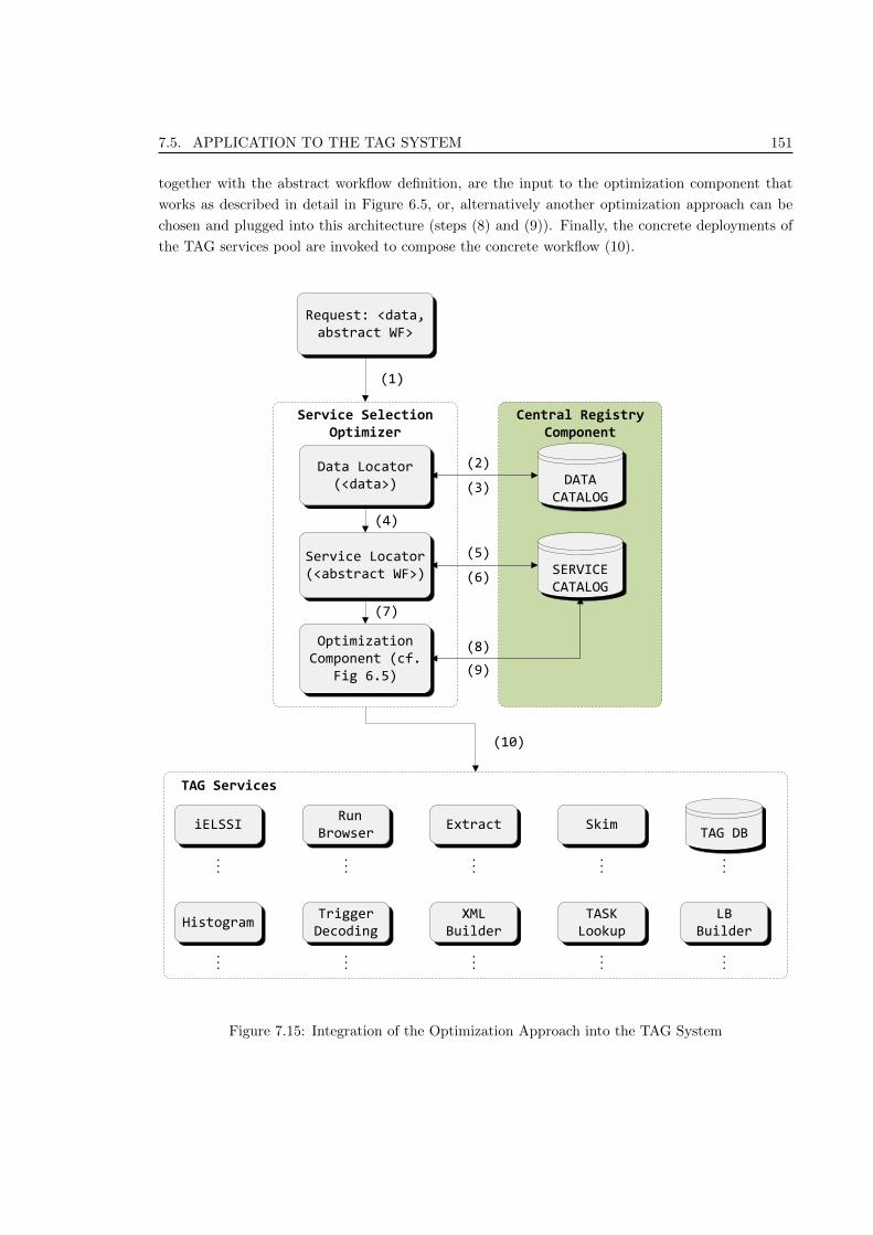
7.5. APPLICATION TO THE TAG SYSTEM 151
together with the abstract workflow definition, are the input to the optimization component that
works as described in detail in Figure 6.5, or, alternatively another optimization approach can be
chosen and plugged into this architecture (steps (8) and (9)). Finally, the concrete deployments of
the TAG services pool are invoked to compose the concrete workflow (10).
(10)
Data Locator (<data>)
Service Locator (<abstract WF>)
Optimization Component (cf.
Fig 6.5)
Service Selection Optimizer
Central Registry Component
DATA CATALOG
SERVICE CATALOG
Request: <data, abstract WF>
(2)
(3)
(5)
(6)
(8)
(9)
(1)
(4)
(7)
iELSSI
TAG Services
TAG DBExtract Skim
TASK Lookup
HistogramTrigger Decoding
XML Builder
LB Builder
Run Browser
......
......
...
......
......
...
Figure 7.15: Integration of the Optimization Approach into the TAG System

152 CHAPTER 7. IMPLEMENTATION AND EVALUATION
7.6 Practical Considerations for the Implementation
As the research carried out in this thesis has been motivated by and applied to a specific application,
it is important to evaluate not only the results, but the entire way of getting to the actual results. In
view of applying a similar methodology to other systems, the operational implications are outlined.
Figure 7.16 summarizes the design and implementation steps followed throughout this work. The
rectangles on the left-hand side depict general steps, those on the right-hand side the specific actions
carried out on the TAG system.
When a centralized optimization approach is added to an already existing system, its design
has to be adapted to work with the system’s components. In the TAG case, the databases and
several of the Web services existed, but were not centrally documented and registered, and the
data distribution was not documented, making it a federation of independent services and data
sources rather than a distributed system. The first step towards a distributed architecture was
the design and implementation of the TASK data catalog as described in Section 4.4, hiding the
data distribution from the users and other applications. The integration of the logging component
and service catalog required contributions from all service developers, because the interface and
internals of each service are different. Therefore, a common API has been defined, but adaptations
were made for each service. As changes in the service’s implementations might have an impact on
their logging component, for instance, these dependencies have to be considered and kept up to
date. Such operational efforts come however with positive “side-effects,” i.e., advantages that have
not originally been planned for. Examples are listed in the following:
• The registry acts as a “dynamic” (or “self-adaptive”) documentation of the system.
• The data in the registry allows having detailed knowledge about the status of any system
component at any time. The tracking of changes allows documenting the evolution of the
system components. This further allows noticing trends, for example the degradation of a
usage or performance index that might indicate intrinsic errors.
• The logging information can be further used to mine data about the system usage.
• The central registry (in the TAG case the TASK Service Catalog) can be used as a repository
for service configurations, therefore allowing an automated configuration management (on a
basic level, not to be confounded with dedicated configuration management tools).
Based on the experience of implementing and operating a knowledge base and service discovery
mechanism in the TAG system, the following recommendations can be made:
• If possible, it is evidently beneficial to include service discovery and selection in the initial
system design.
• In a distributed system involving developers from different organizations and locations, it is
important to have a strong commitment for a centralized service selection approach.
• If a rather small system is deployed, but it is expected to grow in terms of number of ser-
vices and deployments, a flexible optimization framework allowing plugging in different service

7.6. PRACTICAL CONSIDERATIONS FOR THE IMPLEMENTATION 153
selection algorithms is desirable. This way, depending on the size of the system, different
algorithms can be run.
• The operations of the registry and other components related to the service selection should be
part of the general system’s operations.
General steps Example: TAG system
1. Design and Implementation of a registry for service discovery
TASK Catalogs and APIs (Chap. 4)
2. Implementation of services logging and system monitoring
3. Identification of relevant QoS attributes and aggregated metrics
4. Analysis of the dynamic aspects, change frequencies, etc. using the logging information
5. Design and Implement an appropriate optimization approach
6. Evaluation and tuning of the approach
7. Test deployment
8. Production deployment
9. Monitoring and observation of evolving attributes, usage patterns, user satisfaction, e tc.
TAG Logging & Aggregation (Chap. 4)
Definition of QoSattributes in TASK
(Chap. 4)
Analysis carried out in Chap. 5
Optimization approach (AD-MOGA) presented in Chap. 6
Evaluation presented in Chap. 7, and
ongoing operations
Feed
bac
k Lo
op
Figure 7.16: Outline of Design and Implementation Steps

154 CHAPTER 7. IMPLEMENTATION AND EVALUATION
7.7 Possible Extensions in Future Work
The presented optimization framework is self-contained and can be deployed as it is. However, there
are several areas of possible enhancements and extensions that make the overall approach more fine
grained, robust, and allow for a wider scope. The identified areas are schematically represented in
Figure 7.17 and described in the following:
Algorithmic Approaches. In the proposed approach, a GA is at the heart of the optimization. It
has been shown that it is particularly suited for dynamic service selection problems. However,
its usefulness depends on the size of the problem. For very small problems, e.g., with five
services having two deployments each, an exhaustive search algorithm is a better option and, as
opposed to a heuristic, guarantees returning the optimal solution. Additionally, the approaches
presented in Chapter 3, Section 3.4, can be prototyped and included as possible available
optimization algorithms. Then, depending on the problem size and characteristics, one of the
algorithms can be chosen to optimize the service selection.
QoS Models. In the considered system, performance and usage indexes are considered as the pri-
mary variables that decisions are based on. It could however be useful to carry out simulations
with different aggregated QoS metrics and compare the results, especially in terms of system
throughput. The choice of the “right” QoS metrics to take into account is not trivial and
can be based on simulation results indicating the resulting system behavior. Therefore, in the
same way as different algorithms can be implemented and compared, different QoS models can
be included in the framework.
Fine-grained Weighting. Weights assigned to QoS attributes are another area of possible exten-
sions. Weights can be assigned at different levels in order to refine the preferences during the
deployment selection process. In this work, weights are defined on optimization objectives
through optimization profiles. However, in many systems the assignment can be a more com-
plex process. Weights on attributes can be defined based on the involved abstract services and
the nature of the concrete request. For example, if the invocation of service B from service
A requires data transfer, and a given request is defined on a large amount of data, then the
throughput of the link between service A and service B is more important (has a higher impact)
than its latency. Therefore, mechanisms determining those kinds of weights on the fly, based
on pre-defined attributes and on the analysis of logging information and/or simulation results,
can be designed and implemented.
Model Simulation. Finally, it is important to verify the above-mentioned extensions and model
options through simulation. The system can either be represented in a custom database model,
as in the evaluation carried out in this thesis, or simulation tools such as SimGrid [23] can
be customized and used to build a system model and run specific simulations on it. The
ultimate goal is not only to be able to compare algorithms and QoS models, but also to allow
for system capacity planning. For instance, in terms of planning it is crucial to determine the
consequences of adding or removing deployments (with specific QoS categories). If the overall
performance of a distributed system is degrading due to a high utilization resulting in a high
load on the underlying resources, the issue can be addressed either by optimizing the current

7.8. SUMMARY 155
system setup, or by adding new resources. In a distributed system, it is crucial where to add
a deployment. This question can be addressed by adding a virtual resource to the model and
performing simulation runs of typical workload. This allows building the capacity planning
process on robust decisions.
Aggregating the above-described parts allows building an Anytime Learning System for ad-
dressing QoS-aware service selection problems under different and changing conditions. Anytime
learning refers to a generic approach to continuous learning in a system that changes and evolves
over time [73]. Figure 7.18, derived from the architecture proposed by Ramsey and Grefenstette
in [73], shows a possible anytime learning architecture in this context. It is composed of two main
parts, the execution system and the learning system. In the execution system, a decision maker
interacts with the monitored distributed system and optimizes deployment selections by not only
accessing the service registry containing the QoS metrics, but also an active knowledge base that
stores information about good optimization approaches. This knowledge base can be seen as an
extended version of the persistent memory introduced in Chapter 6. It contains strategies to be
applied to the optimization, depending on the system environment, the nature and frequency of
changes, etc. In the learning system, new strategies (e.g., algorithms, QoS models) are applied and
their impact is evaluated. If a strategy proves to be better than the ones in the execution system,
it is transferred from the test knowledge base to the active knowledge base. The ultimate goals of
applying such an anytime learning system include:
• Decide on the most appropriate algorithmic approach to be applied for deployment selection.
• Decide on QoS models that best reflect the real system.
• Track environmental changes over the system lifetime and derive profiles regarding usage,
optimization, utilization, etc.
• Test and assess changes in the system configuration.
In addition to the above mentioned areas, it is interesting to explore different ways of computing
the similarity index (cf. Chapter 5, Section 5.2.3). The index computation introduced in this thesis
with the goal of providing a quantification of system changes between time t and time t+∆t is a first
attempt, but other approaches can be investigated. The presented index has a few shortcomings.
For example, if a concrete workflow composed of four deployments is considered, each deployment
belonging to a service containing 20 different deployments each, and one deployment per service
changes between t and t + ∆t, the resulting similarity index is high (only 4 changed deployments
out of 80). However, if by coincidence exactly those four deployments making up the previously
computed optimal solution are affected by the changes, then the real impact can be higher than
expressed by the similarity index. It is thus worthwhile to consider such special cases and embed
the similarity computation into a broader framework.
7.8 Summary
The findings of the evaluation of AD-MOGA can be summarized as follows:

156 CHAPTER 7. IMPLEMENTATION AND EVALUATION
Algorithmic Approaches
QoS Models
Fine-grained Weighting
Model Simulation
Anytime Learning and Expert System to address QoS-Aware Service Selection Optimization
Figure 7.17: Areas for Future Extensions
Service-Oriented System
Active Knowledgebase
Monitor
Optimization and Decision Component
Simulation Model
Decision Maker Model
Learning Method Test Knowledgebase
EXECUTION SYSTEM LEARNING SYSTEM
Service Registry
Test Service Registry
Planning Component
Figure 7.18: Anytime Learning System for Service Selection Optimization
• For a set of studied input parameters, AD-MOGA converges towards the Pareto front in a
range of 60 to 100 generations for realistic problem sizes.
• AD-MOGA adapts to changes in the environment by identifying system changes and their im-
pact, and adapting its initialization and its mutation rate accordingly. This results in a quicker
convergence towards the Pareto front, if information from past computation can be reused. If
the system changes radically (similarity index below 0.5), a restart of the optimization with a
random initialization is however preferable.

7.8. SUMMARY 157
• Experiments have shown that the more changes there are, the higher the mutation rate should
be, in order to ensure a high diversity in the population. This is valid up to a change rate of
about 50%, above which a complete random restart is the better option.
• In terms of runtime, AD-MOGA scales well to big but realistic problem sizes. The most
cost-intensive phases in the algorithm are the computation of the overall workflow fitness
(performance and usage) and the identification of the Pareto candidates in each generation.
Therefore, these are areas to focus on for future improvements. Specifically, external math-
ematics packages taking for instance advantage of vectorization techniques can be used to
determine the Pareto candidates.
Those findings are represented in Figure 7.19 in the form of a structured decision tree. The
left-most leaf, called root leaf, is the starting point. The first decision concerns the problem space.
The evaluation showed that for a system setup with 5 services having 20 deployments each, and a
workflow of 5 services, the exhaustive search algorithm is not an option anymore, because its runtime
is of the order of minutes. However, the exact definitions of “big” and “small” have to be evaluated
on a per-scenario basis, which is why those qualitative expressions are kept in the decision tree.
For “big” problem setups, AD-MOGA is used, and the further options – such as random (re)start,
(re)start from memory and adaptation of the mutation rate – depend on the impact of changes
occurring between and during optimization runs.

158 CHAPTER 7. IMPLEMENTATION AND EVALUATION
AD-MOGA
Exact
Algorithm
Random GA
Restart
Random GA
Restart
Start from
Memory,
Mutation
Adaptation
Terminate
GA normally
Replace part
of population
randomly
Adapt
Mutation Rate
during Run
Big problem size
Small problem size
WF and OP(t) in Memory
WF and OP(t) not in Memory
Similarity Index < 0.5
Similarity Index >= 0.5Change during Optimization
No Change during Optimization
Similarity Index < 0.5
Similarity Index >= 0.5
Fig
ure
7.19
:D
ecis
ion
Tre
eS
um
mari
zin
gth
eE
valu
ati
on
Fin
din
gs

Chapter 8
Conclusion
Quality-aware service selection is about choosing concrete services (deployments) for a workflow in
such a way that Quality of Service (QoS) considerations are optimized. This broad topic has become
crucially important with the emergence of large, service-oriented systems, in which an abstract
service usually exists in several, distributed concrete deployments. When instantiating a workflow,
deployments have to be selected and composed at run-time. This thesis work has been motivated
by the service selection challenge arising in a concrete application, the TAG system in the ATLAS
experiment. The TAG system is characterized by a central control instance, tightly coupled services,
a dynamic environment, and changing objectives and priorities. This thesis investigates specific
aspects of the QoS-aware service selection problem and makes three contributions to the research
area:
1. A high-level ontology for describing the components and QoS attributes of service-oriented
systems is proposed. This ontology specifies a vocabulary for describing the elements required
to formulate a service selection optimization problem on a specific system. It is shared between
providers of distributed services and aims at providing a shared understanding of a system. As
opposed to detailed and complete system models, the proposed ontology focuses specifically
on the elements required for the service selection process.
2. QoS-aware service selection is defined as a dynamic, multi-objective optimization problem.
Multiple objectives for such problems are common in related work, but the dynamic aspects
have been neglected in related problem definitions. Starting from the analysis of the dynamics
in the studied TAG application, system and optimization profiles are introduced. These profiles
define the state of the system and the optimization instance at a given point in time. The
optimization itself is carried out from two conflicting perspectives, namely the user’s and
the provider’s perspective. The resulting problem is modeled as a multi-objective, multi-
constrained optimal path problem.
3. A dynamic and adaptive multi-objective genetic algorithm is designed, implemented and eval-
uated. It is tailored to address dynamic QoS-aware service selection problems and efficiently
analyzes the changes in the underlying system to reduce its runtime. Evaluation results demon-
strate the applicability and accuracy of the approach as well as its scalability to systems with
159

160 CHAPTER 8. CONCLUSION
a large number of components and services.
In future work, the optimization framework can be extended towards other algorithmic ap-
proaches, in order to provide a testbed for different algorithms on dynamic service selection prob-
lems. Furthermore, an Anytime Learning System addressing the specific challenges of dynamic
service selection identified in this thesis can be derived. The learning component of such a system
can then both vary adaptation methods of a genetic algorithm, for instance AD-MOGA, and try
different algorithms (defined in the extended optimization framework) to update the knowledge base
used by the decision maker on the execution environment. The simulated environment used in the
evaluation part of this work can serve as a learning system, while the TAG application is a real-world
execution system. The work presented in this thesis is an enabling step in that direction.
For concluding the thesis, I have been asked to formulate seven statements related to the thesis, and
three general statements, as personal reflections:
1. Scientific applications involving data-intensive services are particularly appropriate scenarios
for studying QoS-aware service selection problems.
2. It is more accurate to model the service selection as a constrained optimal path problem than
as a knapsack problem, because neglecting the QoS of links between services considerably
biases the overall workflow QoS.
3. Metaheuristic algorithms are the most promising approaches to real-world service selection
problems, because they scale well to typical problem sizes arising in the World Wide Web.
4. Components of service-oriented systems and their QoS attributes can be precisely defined via
ontologies for a given domain of discourse.
5. The QoS-aware service selection challenge can be formulated as a dynamic multi-objective
optimization problem.
6. A persistent memory and a change tracking system provide an efficient means to leverage the
usage of genetic algorithms to solve dynamic service selection problems.
7. The implementation of a QoS registry and a service selection optimization framework in a
real-world system considerably augments the manageability of the system.
8. Pragmatism is an important attitude while finishing a PhD thesis, and probably any other
mid- and long-term project.
9. The importance given to a thing is a function of the viewpoint and experience one has on the
thing.
10. There is no such thing like music to express the whole spectrum of nuances and colors of reality
and imagination.

Appendix A
System and Attribute Ontology:
OWL Schemas
A.1 OWL Definitions Used in the Ontologies
OWL is a Web Ontology language developed by the World Wide Web Consortium (W3C). It is a
language for knowledge representation based on the Resource Description Framework (RDF), which
is another W3C standard for data exchange on the Web [99]. It is used for describing information
conceptually, and thus acts as a metadata model for a given domain of interest. In the following,
the OWL concepts and constructs used in the system and attribute ontology are shortly described.
The definitions are based on those provided in [48] and [98].
Individual. Individuals are objects from the domain described by the ontology, also referred to as
the domain of discourse. In the example at hand, a service oriented computing system is the
domain of discourse, and objects are instances of servers, services, etc. OWL does not use the
Unique Name Assumption, therefore two individuals must be explicitly defined as being the
same or distinct from each other.
Class. A class is a group of individuals sharing some properties. Classes are organized hierarchically
in a superclass-subclass manner. Subclasses inherit properties from their subclass(es). All
classes are subclasses of the root class Thing. If classes are disjoint, then an individual can
only belong to exactly one of these classes. Defined classes have a precise definition, i.e.,
necessary and sufficient conditions, and any individual that satisfies those conditions belongs
per definition to the class. Classes without such a definition are referred to as primitive classes
– they only have necessary conditions.
Property. Properties are used to model relationships between individuals (object properties) or
between individuals and data types (data properties). Properties can have specified domains
and ranges, i.e., they relate individuals from the domain (class) to individuals from the range
(class). For example, the property hosts links individuals from the class Provider to individ-
uals from the class Resource. The property isHostedBy is the inverse property of hosts and
161

162 APPENDIX A. SYSTEM AND ATTRIBUTE ONTOLOGY: OWL SCHEMAS
domain and range are flipped over. If a property is functional, then every individual can be
linked to only exactly one other individual via this property. If a property is transitive, then
if it relates individual A to individual B and B to C, it can be concluded that it also relates A
to C. If a property that relates A to B necessarily implies that this same property also relates
B to A, then the property is called symmetric. If in turn the fact that a property relates A to
B implies that the same property cannot relate B to A, it is called asymmetric. A property is
called reflexive if it must relate an individual to itself, and irreflexive it if cannot relate an
individual to itself.
Restrictions. A restriction describes a class of individuals based on the relationships that members
of these classes have with other individuals. There are three restriction categories: Quantifier
Restrictions, Cardinality Restrictions and hasValue Restrictions. Quantifier restrictions can
be existential or universal. Existential restrictions describe classes of individuals that have
at least one relationship via a specific property to individuals of a specific class (keyword
some in Protege). Universal restrictions describe classes of individuals that are linked to other
individuals through a given property to only individuals from a specific class (keyword only
in Protege). Cardinality restrictions define the number of relationships an individual has for a
given property (minimum, maximum, exact number). A hasValue restriction defines a class of
individuals that are related to a specific individual with a certain property. Finally, a Closure
Axiom on a property is a universal restriction for this property that restricts the possible
ranges of the property.
A.2 System Ontology: OWL Schema
<?xml ve r s i on=”1.0”?>
<!DOCTYPE Ontology [
<!ENTITY xsd ”http ://www.w3 . org /2001/XMLSchema#” >
<!ENTITY xml ”http ://www.w3 . org /XML/1998/ namespace” >
<!ENTITY rd f s ” http ://www.w3 . org /2000/01/ rdf−schema#” >
<!ENTITY rd f ”http ://www.w3 . org /1999/02/22− rdf−syntax−ns#” >
]>
<Ontology xmlns=”http ://www.w3 . org /2002/07/ owl#”
xml : base=”http ://www. system . com/ on t o l o g i e s / system onto logy . owl”
xmlns : r d f s=”http ://www.w3 . org /2000/01/ rdf−schema#”
xmlns : xsd=”http ://www.w3 . org /2001/XMLSchema#”
xmlns : rd f=”http ://www.w3 . org /1999/02/22− rdf−syntax−ns#”
xmlns : xml=”http ://www.w3 . org /XML/1998/ namespace”
onto logyIRI=”http ://www. system . com/ on t o l o g i e s / system onto logy . owl”>
<Pre f i x name=”xsd” IRI=”http ://www.w3 . org /2001/XMLSchema#”/>
<Pre f i x name=”owl” IRI=”http ://www.w3 . org /2002/07/ owl#”/>
<Pre f i x name=”” IRI=”http ://www.w3 . org /2002/07/ owl#”/>
<Pre f i x name=”rd f ” IRI=”http ://www.w3 . org /1999/02/22− rdf−syntax−ns#”/>
<Pre f i x name=”rd f s ” IRI=”http ://www.w3 . org /2000/01/ rdf−schema#”/>
<Annotation>
<AnnotationProperty abbrev iatedIRI=”rd f s : comment”/>
<L i t e r a l datatypeIRI=”&rd f ; P l a i nL i t e r a l ”>Ontology de s c r i b i n g the bu i l d ing b locks
o f a computing system ( s p e c i f i c a l l y a d i s t r i bu t ed , s e rv i c e−o r i en t ed system )
and t h e i r c h a r a c t e r i s t i c s in form of a t t r i b u t e s .</ L i t e r a l>
</Annotation>
<Declarat ion><Class IRI=”#AbsoluteValueType”/></Dec larat ion>
<Declarat ion><Class IRI=”#Ac c e s s i b i l i t yA t t r i b u t e ”/></Dec larat ion>
<Declarat ion><Class IRI=”#AtomicComponent”/></Dec larat ion>

A.2. SYSTEM ONTOLOGY: OWL SCHEMA 163
<Declarat ion><Class IRI=”#Attr ibute”/></Dec larat ion>
<Declarat ion><Class IRI=”#Attr ibuteDimension”/></Dec larat ion>
<Declarat ion><Class IRI=”#AttributeDynamicType”/></Dec larat ion>
<Declarat ion><Class IRI=”#AttributeMetaData”/></Dec larat ion>
<Declarat ion><Class IRI=”#Attr ibuteValueAcquis i t ionType”/></Dec larat ion>
<Declarat ion><Class IRI=”#AttributeValueDataType”/></Dec larat ion>
<Declarat ion><Class IRI=”#AttributeValueType”/></Dec larat ion>
<Declarat ion><Class IRI=”#Attr ibuteValueUnit”/></Dec larat ion>
<Declarat ion><Class IRI=”#Ava i l a b i l i t yA t t r i bu t e”/></Dec larat ion>
<Declarat ion><Class IRI=”#BandwidthAttribute”/></Dec larat ion>
<Declarat ion><Class IRI=”#CombinedDimension”/></Dec larat ion>
<Declarat ion><Class IRI=”#ComposedComponent”/></Dec larat ion>
<Declarat ion><Class IRI=”#CostAttr ibute”/></Dec larat ion>
<Declarat ion><Class IRI=”#DefinedType”/></Dec larat ion>
<Declarat ion><Class IRI=”#Deployment”/></Dec larat ion>
<Declarat ion><Class IRI=”#DynamicType”/></Dec larat ion>
<Declarat ion><Class IRI=”#EstimatedType”/></Dec larat ion>
<Declarat ion><Class IRI=”#Funct iona lAtt r ibute”/></Dec larat ion>
<Declarat ion><Class IRI=”#LatencyAttr ibute”/></Dec larat ion>
<Declarat ion><Class IRI=”#Link”/></Dec larat ion>
<Declarat ion><Class IRI=”#LoadAttribute”/></Dec larat ion>
<Declarat ion><Class IRI=”#MeasuredType”/></Dec larat ion>
<Declarat ion><Class IRI=”#NonFunct ionalAttr ibute”/></Dec larat ion>
<Declarat ion><Class IRI=”#PredictedType”/></Dec larat ion>
<Declarat ion><Class IRI=”#Provider”/></Dec larat ion>
<Declarat ion><Class IRI=”#QuasiStaticType”/></Dec larat ion>
<Declarat ion><Class IRI=”#RegulatoryAttr ibute”/></Dec larat ion>
<Declarat ion><Class IRI=”#RelativeValueType”/></Dec larat ion>
<Declarat ion><Class IRI=”#Re l i a b i l i t yA t t r i b u t e ”/></Dec larat ion>
<Declarat ion><Class IRI=”#Reputat ionAttr ibute”/></Dec larat ion>
<Declarat ion><Class IRI=”#Resource”/></Dec larat ion>
<Declarat ion><Class IRI=”#RuleValueType”/></Dec larat ion>
<Declarat ion><Class IRI=”#Secur i t yAt t r i bu t e”/></Dec larat ion>
<Declarat ion><Class IRI=”#Serv i c e”/></Dec larat ion>
<Declarat ion><Class IRI=”#SizeDimension”/></Dec larat ion>
<Declarat ion><Class IRI=”#StaticType”/></Dec larat ion>
<Declarat ion><Class IRI=”#System”/></Dec larat ion>
<Declarat ion><Class IRI=”#SystemComponent”/></Dec larat ion>
<Declarat ion><Class IRI=”#ThroughputAttribute”/></Dec larat ion>
<Declarat ion><Class IRI=”#TimeAttribute”/></Dec larat ion>
<Declarat ion><Class IRI=”#TimeDimension”/></Dec larat ion>
<Declarat ion><ObjectProperty IRI=”#con s i s t sO f”/></Dec larat ion>
<Declarat ion><ObjectProperty IRI=”#con s t i t u t e s ”/></Dec larat ion>
<Declarat ion><ObjectProperty IRI=”#hasAttr ibute”/></Dec larat ion>
<Declarat ion><ObjectProperty IRI=”#hasDeployment”/></Dec larat ion>
<Declarat ion><ObjectProperty IRI=”#hasDimension”/></Dec larat ion>
<Declarat ion><ObjectProperty IRI=”#hasDynamicType”/></Dec larat ion>
<Declarat ion><ObjectProperty IRI=”#hasMetaData”/></Dec larat ion>
<Declarat ion><ObjectProperty IRI=”#hasValueUnit”/></Dec larat ion>
<Declarat ion><ObjectProperty IRI=”#hasValueAcquis it ionType”/></Dec larat ion>
<Declarat ion><ObjectProperty IRI=”#hasValueDataType”/></Dec larat ion>
<Declarat ion><ObjectProperty IRI=”#hasValueType”/></Dec larat ion>
<Declarat ion><ObjectProperty IRI=”#host s”/></Dec larat ion>
<Declarat ion><ObjectProperty IRI=”#i sAt t r ibu t eOf”/></Dec larat ion>
<Declarat ion><ObjectProperty IRI=”#isDeploymentOf”/></Dec larat ion>
<Declarat ion><ObjectProperty IRI=”#isHostedBy”/></Dec larat ion>
<Declarat ion><ObjectProperty IRI=”#l i n k s ”/></Dec larat ion>
<Declarat ion><DataProperty IRI=”#hasID”/></Dec larat ion>
<Declarat ion><DataProperty IRI=”#hasName”/></Dec larat ion>
<Declarat ion><DataProperty IRI=”#isAtomic”/></Dec larat ion>
<Equiva lentClasses>
<Class IRI=”#AtomicComponent”/>
<Objec t Inte r s ec t i onOf>

164 APPENDIX A. SYSTEM AND ATTRIBUTE ONTOLOGY: OWL SCHEMAS
<Class IRI=”#SystemComponent”/>
<DataHasValue>
<DataProperty IRI=”#isAtomic”/>
<L i t e r a l datatypeIRI=”&xsd ; boolean”>true</L i t e r a l>
</DataHasValue>
</Objec t Inte r s ec t i onOf>
</Equiva lentClasses>
<Equiva lentClasses>
<Class IRI=”#ComposedComponent”/>
<Objec t Inte r s ec t i onOf>
<Class IRI=”#SystemComponent”/>
<DataHasValue>
<DataProperty IRI=”#isAtomic”/>
<L i t e r a l datatypeIRI=”&xsd ; boolean”> f a l s e </L i t e r a l>
</DataHasValue>
</Objec t Inte r s ec t i onOf>
</Equiva lentClasses>
<Equiva lentClasses>
<Class IRI=”#Deployment”/>
<Objec t Inte r s ec t i onOf>
<Class IRI=”#SystemComponent”/>
<ObjectExactCard ina l i ty c a r d i n a l i t y=”1”>
<ObjectProperty IRI=”#isDeploymentOf”/>
<Objec t Inte r s ec t i onOf>
<Class IRI=”#Resource”/>
<Class IRI=”#Serv i c e ”/>
</Objec t Inte r s ec t i onOf>
</ObjectExactCardinal i ty>
</Objec t Inte r s ec t i onOf>
</Equiva lentClasses>
<Equiva lentClasses>
<Class IRI=”#Link”/>
<Objec t Inte r s ec t i onOf>
<Class IRI=”#SystemComponent”/>
<ObjectMinCardinal i ty c a r d i n a l i t y=”1”>
<ObjectProperty IRI=”#l i n k s ”/>
</ObjectMinCardinal ity>
</Objec t Inte r s ec t i onOf>
</Equiva lentClasses>
<Equiva lentClasses>
<Class IRI=”#Provider”/>
<Objec t Inte r s ec t i onOf>
<Class IRI=”#SystemComponent”/>
<ObjectMinCardinal i ty c a r d i n a l i t y=”1”>
<ObjectProperty IRI=”#host s”/>
</ObjectMinCardinal ity>
</Objec t Inte r s ec t i onOf>
</Equiva lentClasses>
<Equiva lentClasses>
<Class IRI=”#Resource”/>
<Objec t Inte r s ec t i onOf>
<Class IRI=”#SystemComponent”/>
<ObjectExactCard ina l i ty c a r d i n a l i t y=”1”>
<ObjectProperty IRI=”#isHostedBy”/>
</ObjectExactCardinal i ty>
</Objec t Inte r s ec t i onOf>
</Equiva lentClasses>
<SubClassOf>
<Class IRI=”#AbsoluteValueType”/>
<Class IRI=”#AttributeValueType”/>
</SubClassOf>
<SubClassOf>
<Class IRI=”#Ac c e s s i b i l i t yA t t r i b u t e ”/>

A.2. SYSTEM ONTOLOGY: OWL SCHEMA 165
<Class IRI=”#NonFunct ionalAttr ibute”/>
</SubClassOf>
<SubClassOf>
<Class IRI=”#Attr ibute”/>
<Objec t Inte r s ec t i onOf>
<ObjectSomeValuesFrom>
<ObjectProperty IRI=”#hasDimension”/>
<Class IRI=”#Attr ibuteDimension”/>
</ObjectSomeValuesFrom>
<ObjectSomeValuesFrom>
<ObjectProperty IRI=”#hasDynamicType”/>
<Class IRI=”#AttributeDynamicType”/>
</ObjectSomeValuesFrom>
<ObjectSomeValuesFrom>
<ObjectProperty IRI=”#hasMetaData”/>
<Class IRI=”#AttributeMetaData”/>
</ObjectSomeValuesFrom>
<ObjectSomeValuesFrom>
<ObjectProperty IRI=”#hasValueAcquis it ionType”/>
<Class IRI=”#Attr ibuteValueAcquis i t ionType”/>
</ObjectSomeValuesFrom>
<ObjectSomeValuesFrom>
<ObjectProperty IRI=”#hasValueDataType”/>
<Class IRI=”#AttributeValueDataType”/>
</ObjectSomeValuesFrom>
<ObjectSomeValuesFrom>
<ObjectProperty IRI=”#hasValueType”/>
<Class IRI=”#AttributeValueType”/>
</ObjectSomeValuesFrom>
</Objec t Inte r s ec t i onOf>
</SubClassOf>
<SubClassOf><Class IRI=”#AttributeDynamicType”/>
<Class abbrev iatedIRI=”:Thing”/></SubClassOf>
<SubClassOf><Class IRI=”#Attr ibuteValueAcquis i t ionType”/>
<Class abbrev iatedIRI=”:Thing”/></SubClassOf>
<SubClassOf><Class IRI=”#AttributeValueType”/>
<Class abbrev iatedIRI=”:Thing”/></SubClassOf>
<SubClassOf><Class IRI=”#Ava i l a b i l i t yA t t r i bu t e ”/>
<Class IRI=”#NonFunct ionalAttr ibute”/></SubClassOf>
<SubClassOf><Class IRI=”#BandwidthAttribute”/>
<Class IRI=”#NonFunct ionalAttr ibute”/></SubClassOf>
<SubClassOf><Class IRI=”#CombinedDimension”/>
<Class IRI=”#Attr ibuteDimension”/></SubClassOf>
<SubClassOf><Class IRI=”#CostAttr ibute”/>
<Class IRI=”#NonFunct ionalAttr ibute”/></SubClassOf>
<SubClassOf><Class IRI=”#DefinedType”/>
<Class IRI=”#Attr ibuteValueAcquis i t ionType”/></SubClassOf>
<SubClassOf><Class IRI=”#DynamicType”/>
<Class IRI=”#AttributeDynamicType”/></SubClassOf>
<SubClassOf><Class IRI=”#EstimatedType”/>
<Class IRI=”#Attr ibuteValueAcquis i t ionType”/></SubClassOf>
<SubClassOf><Class IRI=”#Funct iona lAtt r ibute”/>
<Class IRI=”#Attr ibute”/></SubClassOf>
<SubClassOf><Class IRI=”#LatencyAttr ibute”/>
<Class IRI=”#NonFunct ionalAttr ibute”/></SubClassOf>
<SubClassOf><Class IRI=”#LoadAttribute”/>
<Class IRI=”#NonFunct ionalAttr ibute”/></SubClassOf>
<SubClassOf><Class IRI=”#MeasuredType”/>
<Class IRI=”#Attr ibuteValueAcquis i t ionType”/></SubClassOf>
<SubClassOf><Class IRI=”#NonFunct ionalAttr ibute”/>
<Class IRI=”#Attr ibute”/></SubClassOf>
<SubClassOf><Class IRI=”#PredictedType”/>
<Class IRI=”#Attr ibuteValueAcquis i t ionType”/></SubClassOf>

166 APPENDIX A. SYSTEM AND ATTRIBUTE ONTOLOGY: OWL SCHEMAS
<SubClassOf><Class IRI=”#QuasiStaticType”/>
<Class IRI=”#AttributeDynamicType”/></SubClassOf>
<SubClassOf><Class IRI=”#RegulatoryAttr ibute”/>
<Class IRI=”#NonFunct ionalAttr ibute”/></SubClassOf>
<SubClassOf><Class IRI=”#RelativeValueType”/>
<Class IRI=”#AttributeValueType”/></SubClassOf>
<SubClassOf><Class IRI=”#Re l i a b i l i t yA t t r i b u t e ”/>
<Class IRI=”#NonFunct ionalAttr ibute”/></SubClassOf>
<SubClassOf><Class IRI=”#Reputat ionAttr ibute”/>
<Class IRI=”#NonFunct ionalAttr ibute”/></SubClassOf>
<SubClassOf><Class IRI=”#RuleValueType”/>
<Class IRI=”#AttributeValueType”/></SubClassOf>
<SubClassOf><Class IRI=”#Secur i t yAt t r i bu t e”/>
<Class IRI=”#NonFunct ionalAttr ibute”/></SubClassOf>
<SubClassOf><Class IRI=”#Serv i c e ”/>
<Class IRI=”#SystemComponent”/></SubClassOf>
<SubClassOf><Class IRI=”#SizeDimension”/>
<Class IRI=”#Attr ibuteDimension”/></SubClassOf>
<SubClassOf><Class IRI=”#StaticType”/>
<Class IRI=”#AttributeDynamicType”/></SubClassOf>
<SubClassOf>
<Class IRI=”#SystemComponent”/>
<DataExactCardinal i ty c a r d i n a l i t y=”1”>
<DataProperty IRI=”#isAtomic”/>
<Datatype abbrev iatedIRI=”xsd : boolean”/>
</DataExactCardinal ity>
</SubClassOf>
<SubClassOf><Class IRI=”#ThroughputAttribute”/>
<Class IRI=”#NonFunct ionalAttr ibute”/></SubClassOf>
<SubClassOf><Class IRI=”#TimeAttribute”/>
<Class IRI=”#NonFunct ionalAttr ibute”/></SubClassOf>
<SubClassOf><Class IRI=”#TimeDimension”/>
<Class IRI=”#Attr ibuteDimension”/></SubClassOf>
<Di s j o i n tC l a s s e s><Class IRI=”#Funct iona lAtt r ibute”/>
<Class IRI=”#NonFunct ionalAttr ibute”/></D i s j o i n tC l a s s e s>
<Inve r s eObjec tPrope r t i e s><ObjectProperty IRI=”#con s i s t sO f ”/>
<ObjectProperty IRI=”#con s t i t u t e s ”/></Inve r s eObjec tProper t i e s>
<Inve r s eObjec tPrope r t i e s><ObjectProperty IRI=”#hasAttr ibute”/>
<ObjectProperty IRI=”#i sAt t r ibu t eOf”/></Inve r s eObjec tProper t i e s>
<Inve r s eObjec tPrope r t i e s><ObjectProperty IRI=”#hasDeployment”/>
<ObjectProperty IRI=”#isDeploymentOf”/></Inve r s eObjec tProper t i e s>
<Inve r s eObjec tPrope r t i e s><ObjectProperty IRI=”#host s”/>
<ObjectProperty IRI=”#isHostedBy”/></Inve r s eObjec tProper t i e s>
<Funct ionalObjectProperty>
<ObjectProperty IRI=”#hasDimension”/>
</Funct ionalObjectProperty>
<Funct ionalObjectProperty>
<ObjectProperty IRI=”#hasDynamicType”/>
</Funct ionalObjectProperty>
<Funct ionalObjectProperty>
<ObjectProperty IRI=”#hasMetaData”/>
</Funct ionalObjectProperty>
<Funct ionalObjectProperty>
<ObjectProperty IRI=”#hasValueAcquis it ionType”/>
</Funct ionalObjectProperty>
<Funct ionalObjectProperty>
<ObjectProperty IRI=”#hasValueDataType”/>
</Funct ionalObjectProperty>
<Funct ionalObjectProperty>
<ObjectProperty IRI=”#hasValueType”/>
</Funct ionalObjectProperty>
<Funct ionalObjectProperty>
<ObjectProperty IRI=”#isDeploymentOf”/>
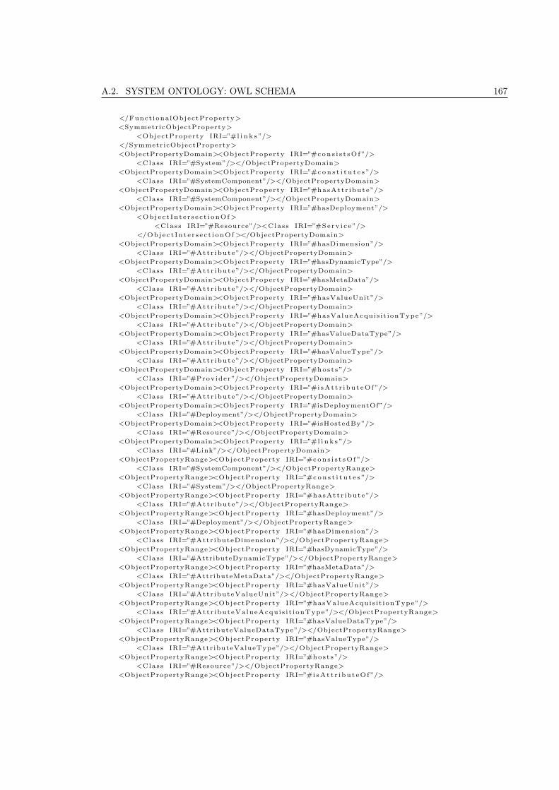
A.2. SYSTEM ONTOLOGY: OWL SCHEMA 167
</Funct ionalObjectProperty>
<SymmetricObjectProperty>
<ObjectProperty IRI=”#l i n k s ”/>
</SymmetricObjectProperty>
<ObjectPropertyDomain><ObjectProperty IRI=”#con s i s t sO f ”/>
<Class IRI=”#System”/></ObjectPropertyDomain>
<ObjectPropertyDomain><ObjectProperty IRI=”#con s t i t u t e s ”/>
<Class IRI=”#SystemComponent”/></ObjectPropertyDomain>
<ObjectPropertyDomain><ObjectProperty IRI=”#hasAttr ibute”/>
<Class IRI=”#SystemComponent”/></ObjectPropertyDomain>
<ObjectPropertyDomain><ObjectProperty IRI=”#hasDeployment”/>
<Objec t Inte r s ec t i onOf>
<Class IRI=”#Resource”/><Class IRI=”#Serv i c e ”/>
</Objec t Inte r s ec t i onOf></ObjectPropertyDomain>
<ObjectPropertyDomain><ObjectProperty IRI=”#hasDimension”/>
<Class IRI=”#Attr ibute”/></ObjectPropertyDomain>
<ObjectPropertyDomain><ObjectProperty IRI=”#hasDynamicType”/>
<Class IRI=”#Attr ibute”/></ObjectPropertyDomain>
<ObjectPropertyDomain><ObjectProperty IRI=”#hasMetaData”/>
<Class IRI=”#Attr ibute”/></ObjectPropertyDomain>
<ObjectPropertyDomain><ObjectProperty IRI=”#hasValueUnit”/>
<Class IRI=”#Attr ibute”/></ObjectPropertyDomain>
<ObjectPropertyDomain><ObjectProperty IRI=”#hasValueAcquis it ionType”/>
<Class IRI=”#Attr ibute”/></ObjectPropertyDomain>
<ObjectPropertyDomain><ObjectProperty IRI=”#hasValueDataType”/>
<Class IRI=”#Attr ibute”/></ObjectPropertyDomain>
<ObjectPropertyDomain><ObjectProperty IRI=”#hasValueType”/>
<Class IRI=”#Attr ibute”/></ObjectPropertyDomain>
<ObjectPropertyDomain><ObjectProperty IRI=”#host s”/>
<Class IRI=”#Provider”/></ObjectPropertyDomain>
<ObjectPropertyDomain><ObjectProperty IRI=”#i sAt t r ibu t eOf”/>
<Class IRI=”#Attr ibute”/></ObjectPropertyDomain>
<ObjectPropertyDomain><ObjectProperty IRI=”#isDeploymentOf”/>
<Class IRI=”#Deployment”/></ObjectPropertyDomain>
<ObjectPropertyDomain><ObjectProperty IRI=”#isHostedBy”/>
<Class IRI=”#Resource”/></ObjectPropertyDomain>
<ObjectPropertyDomain><ObjectProperty IRI=”#l i n k s ”/>
<Class IRI=”#Link”/></ObjectPropertyDomain>
<ObjectPropertyRange><ObjectProperty IRI=”#con s i s t sO f ”/>
<Class IRI=”#SystemComponent”/></ObjectPropertyRange>
<ObjectPropertyRange><ObjectProperty IRI=”#con s t i t u t e s ”/>
<Class IRI=”#System”/></ObjectPropertyRange>
<ObjectPropertyRange><ObjectProperty IRI=”#hasAttr ibute”/>
<Class IRI=”#Attr ibute”/></ObjectPropertyRange>
<ObjectPropertyRange><ObjectProperty IRI=”#hasDeployment”/>
<Class IRI=”#Deployment”/></ObjectPropertyRange>
<ObjectPropertyRange><ObjectProperty IRI=”#hasDimension”/>
<Class IRI=”#Attr ibuteDimension”/></ObjectPropertyRange>
<ObjectPropertyRange><ObjectProperty IRI=”#hasDynamicType”/>
<Class IRI=”#AttributeDynamicType”/></ObjectPropertyRange>
<ObjectPropertyRange><ObjectProperty IRI=”#hasMetaData”/>
<Class IRI=”#AttributeMetaData”/></ObjectPropertyRange>
<ObjectPropertyRange><ObjectProperty IRI=”#hasValueUnit”/>
<Class IRI=”#Attr ibuteValueUnit”/></ObjectPropertyRange>
<ObjectPropertyRange><ObjectProperty IRI=”#hasValueAcquis it ionType”/>
<Class IRI=”#Attr ibuteValueAcquis i t ionType”/></ObjectPropertyRange>
<ObjectPropertyRange><ObjectProperty IRI=”#hasValueDataType”/>
<Class IRI=”#AttributeValueDataType”/></ObjectPropertyRange>
<ObjectPropertyRange><ObjectProperty IRI=”#hasValueType”/>
<Class IRI=”#AttributeValueType”/></ObjectPropertyRange>
<ObjectPropertyRange><ObjectProperty IRI=”#host s”/>
<Class IRI=”#Resource”/></ObjectPropertyRange>
<ObjectPropertyRange><ObjectProperty IRI=”#i sAt t r ibu t eOf”/>

168 APPENDIX A. SYSTEM AND ATTRIBUTE ONTOLOGY: OWL SCHEMAS
<Class IRI=”#SystemComponent”/></ObjectPropertyRange>
<ObjectPropertyRange><ObjectProperty IRI=”#isDeploymentOf”/>
<Objec t Inte r s ec t i onOf>
<Class IRI=”#Resource”/><Class IRI=”#Serv i c e ”/>
</Objec t Inte r s ec t i onOf></ObjectPropertyRange>
<ObjectPropertyRange><ObjectProperty IRI=”#isHostedBy”/>
<Class IRI=”#Provider”/></ObjectPropertyRange>
<ObjectPropertyRange><ObjectProperty IRI=”#l i n k s ”/>
<ObjectUnionOf>
<Class IRI=”#Deployment”/><Class IRI=”#Provider”/><Class IRI=”#Resource”/>
</ObjectUnionOf></ObjectPropertyRange>
<FunctionalDataProperty>
<DataProperty IRI=”#hasID”/>
</FunctionalDataProperty>
<FunctionalDataProperty>
<DataProperty IRI=”#hasName”/>
</FunctionalDataProperty>
<FunctionalDataProperty>
<DataProperty IRI=”#isAtomic”/>
</FunctionalDataProperty>
<DataPropertyDomain><DataProperty IRI=”#hasID”/>
<Class IRI=”#Attr ibute”/></DataPropertyDomain>
<DataPropertyDomain><DataProperty IRI=”#hasID”/>
<Class IRI=”#SystemComponent”/></DataPropertyDomain>
<DataPropertyDomain><DataProperty IRI=”#hasName”/>
<Class IRI=”#Attr ibute”/></DataPropertyDomain>
<DataPropertyDomain><DataProperty IRI=”#hasName”/>
<Class IRI=”#SystemComponent”/></DataPropertyDomain>
<DataPropertyDomain><DataProperty IRI=”#isAtomic”/>
<Class IRI=”#SystemComponent”/></DataPropertyDomain>
<DataPropertyRange><DataProperty IRI=”#hasID”/>
<Datatype abbrev iatedIRI=”rd f s : L i t e r a l ”/></DataPropertyRange>
<DataPropertyRange><DataProperty IRI=”#hasName”/>
<Datatype abbrev iatedIRI=”rd f s : L i t e r a l ”/></DataPropertyRange>
<DataPropertyRange><DataProperty IRI=”#isAtomic”/>
<DataOneOf>
<L i t e r a l datatypeIRI=”&xsd ; boolean”> f a l s e </L i t e r a l>
<L i t e r a l datatypeIRI=”&xsd ; boolean”>true</L i t e r a l>
</DataOneOf></DataPropertyRange>
<Annotat ionAssert ion>
<AnnotationProperty abbrev iatedIRI=”rd f s : comment”/>
<IRI>#AtomicComponent</IRI>
<L i t e r a l datatypeIRI=”&rd f ; P l a i nL i t e r a l ”>Component that , in the context o f the
ontology , cannot be f u r t h e r decomposed in to sma l l e r components .</ L i t e r a l>
</Annotat ionAssert ion>
<Annotat ionAssert ion>
<AnnotationProperty abbrev iatedIRI=”rd f s : comment”/>
<IRI>#Attr ibute</IRI>
<L i t e r a l datatypeIRI=”&rd f ; P l a i nL i t e r a l ”>Thing de s c r i b i ng ( c h a r a c t e r i z i n g ) a
SystemComponent f u n c t i o n a l l y or non−f u n c t i o n a l l y .</ L i t e r a l>
</Annotat ionAssert ion>
<Annotat ionAssert ion>
<AnnotationProperty abbrev iatedIRI=”rd f s : comment”/>
<IRI>#ComposedComponent</IRI>
<L i t e r a l datatypeIRI=”&rd f ; P l a i nL i t e r a l ”>Component that , in the context o f the
ontology , i s composed o f at l e a s t two i nd i v i du a l s o f the c l a s s
AtomicComponent.</ L i t e r a l>
</Annotat ionAssert ion>
<Annotat ionAssert ion>
<AnnotationProperty abbrev iatedIRI=”rd f s : comment”/>
<IRI>#Deployment</IRI>
<L i t e r a l datatypeIRI=”&rd f ; P l a i nL i t e r a l ”>Ins tance o f a s e r v i c e running on a
r e sou r c e . I t i s a conc re t e p i e c e o f so f tware that can be invoked over the

A.2. SYSTEM ONTOLOGY: OWL SCHEMA 169
network .</ L i t e r a l>
</Annotat ionAssert ion>
<Annotat ionAssert ion>
<AnnotationProperty abbrev iatedIRI=”rd f s : comment”/>
<IRI>#Funct iona lAttr ibute</IRI>
<L i t e r a l datatypeIRI=”&rd f ; P l a i nL i t e r a l ”>Attr ibute d e s c r i b i ng the f un c t i ona l
a spec t s o f a SystemComponent . I t d e s c r i b e s WHAT a component ach ieves , as
opposed to how i t i s ach i ev ing i t .</ L i t e r a l>
</Annotat ionAssert ion>
<Annotat ionAssert ion>
<AnnotationProperty abbrev iatedIRI=”rd f s : comment”/>
<IRI>#Link</IRI>
<L i t e r a l datatypeIRI=”&rd f ; P l a i nL i t e r a l ”>Network connect ion between two phys i c a l
system components a l l ow ing ac c e s s or from component A to component B. I t i s
de f ined on the phy s i c a l component l e v e l , because depending on the aimed
g r anu l a r i t y i t can be de f ined between prov iders , r e source s , or
deployments .</ L i t e r a l>
</Annotat ionAssert ion>
<Annotat ionAssert ion>
<AnnotationProperty abbrev iatedIRI=”rd f s : comment”/>
<IRI>#NonFunctionalAttr ibute</IRI>
<L i t e r a l datatypeIRI=”&rd f ; P l a i nL i t e r a l ”>Attr ibute d e s c r i b i ng the non−f un c t i o na l
a spec t s o f a SystemComponent . I t d e s c r i b e s HOW a component i s ach i ev ing
something , as opposed to what i t i s ach i ev ing . Also known as QoS
a t t r i bu t e .</ L i t e r a l>
</Annotat ionAssert ion>
<Annotat ionAssert ion>
<AnnotationProperty abbrev iatedIRI=”rd f s : comment”/>
<IRI>#Provider</IRI>
<L i t e r a l datatypeIRI=”&rd f ; P l a i nL i t e r a l ”>(V i r tua l ) o r gan i za t i on hos t ing at l e a s t
one r e sou r c e that i s part o f the system of i n t e r e s t .</ L i t e r a l>
</Annotat ionAssert ion>
<Annotat ionAssert ion>
<AnnotationProperty abbrev iatedIRI=”rd f s : comment”/>
<IRI>#Resource</IRI>
<L i t e r a l datatypeIRI=”&rd f ; P l a i nL i t e r a l ”>Phys i ca l or l o g i c a l en t i t y capable o f
hos t ing a s e r v i c e . Examples inc lude web se rve r s , database s e r v e r or v i r t u a l
machine . Resources can be nested , e . g . , a v i r t u a l r e sou r c e can run on a
phys i c a l r e s ou r c e .</ L i t e r a l>
</Annotat ionAssert ion>
<Annotat ionAssert ion>
<AnnotationProperty abbrev iatedIRI=”rd f s : comment”/>
<IRI>#Serv ice</IRI>
<L i t e r a l datatypeIRI=”&rd f ; P l a i nL i t e r a l ”>Abstract , s e l f−conta ined f u n c t i o n a l i t y
that can be provided as a p i e c e o f so f tware as a standa lone app l i c a t i on and
that might be composable with other s e r v i c e s .</ L i t e r a l>
</Annotat ionAssert ion>
<Annotat ionAssert ion>
<AnnotationProperty abbrev iatedIRI=”rd f s : comment”/>
<IRI>#System</IRI>
<L i t e r a l datatypeIRI=”&rd f ; P l a i nL i t e r a l ”>A Computing System composed o f s e v e r a l
components that can act toge the r to prov ide some de f ined f u n c t i o n a l i t y to
us e r s i n t e r a c t i n g with the system , be i t humans or other systems .</ L i t e r a l>
</Annotat ionAssert ion>
<Annotat ionAssert ion>
<AnnotationProperty abbrev iatedIRI=”rd f s : comment”/>
<IRI>#SystemComponent</IRI>
<L i t e r a l datatypeIRI=”&rd f ; P l a i nL i t e r a l ”>Log i ca l or phy s i c a l bu i l d ing block o f a
system.</ L i t e r a l>
</Annotat ionAssert ion>
<Annotat ionAssert ion>
<AnnotationProperty abbrev iatedIRI=”rd f s : comment”/>
<IRI>#hasID</IRI>

170 APPENDIX A. SYSTEM AND ATTRIBUTE ONTOLOGY: OWL SCHEMAS
<L i t e r a l datatypeIRI=”&rd f ; P l a i nL i t e r a l ”>Each in s tance o f a SystemComponent has
exac t l y one unique i d e n t i f i e r .</ L i t e r a l>
</Annotat ionAssert ion>
<Annotat ionAssert ion>
<AnnotationProperty abbrev iatedIRI=”rd f s : comment”/>
<IRI>#hasName</IRI>
<L i t e r a l datatypeIRI=”&rd f ; P l a i nL i t e r a l ”>Each i nd i v i dua l in the onto logy has to
have exac t l y one name.</ L i t e r a l>
</Annotat ionAssert ion>
<Annotat ionAssert ion>
<AnnotationProperty abbrev iatedIRI=”rd f s : comment”/>
<IRI>#isAtomic</IRI>
<L i t e r a l datatypeIRI=”&rd f ; P l a i nL i t e r a l ”>d e f i n e s i f a SystemComponent i s atomic
or composed.</ L i t e r a l>
</Annotat ionAssert ion>
<DatatypeDef in i t ion>
<Datatype abbrev iatedIRI=”xsd : boolean”/>
<Datatype abbrev iatedIRI=”xsd : boolean”/>
</DatatypeDef in i t ion>
</Ontology>
<!−− Generated by the OWL API ( ve r s i on 3 . 2 . 3 . 1 7 9 9 ) http :// owlapi . s ou r c e f o r g e . net −−>

Glossary
ACO Ant Colony Optimization. 44
AD-MOGA Adaptive and Dynamic Multi-Objective Genetic Algorithm. 7
AMI tag Refers to a version tag that is part of a dataset name and allows tracking the soft-
ware version and configuration used to produce the dataset. For example, in the dataset
data11 7TeV.00184169.physics MinBias.merge.TAG.f387 m897 m896, the last part namely,
the string f387 m897 m896, is the AMI tag. Not to be confounded with the data product TAG
and the TAG system studied in the context of this work. 71
ANN Artificial Neural Network. 45
AOD Analysis Object Data. Refers to a reduced event representation (output of the data recon-
struction process), derived from ESD, suitable for most physics analyses. 15
ATLAS A Torroidal LHC Apparatus. One of the four large “experiments” (detectors) at the Large
Hadron Collider. 1
BB Branch-and-Bound. 39
CERN Organisation Europeenne pour la Recherche Nucleaire (European Organization for Nuclear
Research). 4
Collection Is a structure developed by ATLAS as part of the POOL framework. POOL collections
are data structures for event data that can be stored in both ROOT and relational formats.
16
DAG Directed Acyclic Graph. 38
dataset Refers to a set of data grouped together. The most common grouping is based on physics
stream, run and data type.
For example, data11 7TeV.00184169.physics MinBias.merge.TAG.f387 m897 m896 is the
name of a dataset grouping TAG data (events) from the MinBias stream in run 184169. 71
EA Evolutionary Algorithm. 43
171

172 GLOSSARY
ESD Event Summary Data. Refers to event data written as first output of the data reconstruction
process, taking RAW data as input. 15
Event In particle physics, an event refers to a collision instance and its set of particle interactions
and intermediate as well as stable products. 13
Event Filter Last element of the ATLAS trigger system. As such, it is the source of real data from
the ATLAS detector. 15
GA Genetic Algorithm. 9
GLG Geometric Location Guided. 41
GUID Globally Unique Identifier, refers to a unique identifier of a file on the Grid. GUIDs can be
dereferenced to physical file locations using a metadata catalog lookup. 17
HEP High Energy Physics. 1
iELSSI interactive Event Level Selection Service Interface. iELSSI is a TAG service that allows
browsing the TAG databases on the Web. 20
LHC Large Hadron Collider. 1
LP Linear Programming. 38
LRA Local Resource Amplest. 41
Lumiblock Time interval (in practice one to two minutes) during which luminosity and detector
conditions can be assumed stable. It is used as granularity in data taking and processing. 20
MCOP Multiconstraint Optimal Path Problem. 3
MIP Mixed Integer Programming. 37
MMKP Multi-dimension Multi-choice Knapsack Problem. 2
MOGA Multi-Objective Genetic Algorithm. 106
MOOP Multi-Objective Optimization Problem. 47
NSGA-II Nondominated Sorting Genetic Algorithm II. 125
OWL Web Ontology Language. 53
POOL Pool Of persistent Objects for LHC. POOL is a hybrid technology store for C++ objects,
using a mixture of streaming and relational technologies to implement both object persistency
and object metadata catalogs and collections. It provides generic components that allow
isolating applications from the storage technology used [82]. 16

GLOSSARY 173
PSO Particle Swarm Optimization. 44
QEP Query Execution Plan. 29
QoS Quality of Service. 2
RAW Collision data (in byte stream format) as it is written as output from the particle detector,
here ATLAS. 13
RDF Resource Description Framework. 161
Reprocessing Refers to the process of reconstructing previously taken RAW data with improved
reconstruction software and calibration constants. This results in a new version of data, called
reprocessed data. 17
ROOT Is a framework for data processing developed at CERN. It allows processing, accessing
and saving data and any C++ object in a compressed binary form, and to show results in
histograms, scatter plots, etc. ROOT provides a data structure that is extremely powerful for
fast access of huge amounts of data [5]. 15
Run Period of data taking, usually defined by the duration of an LHC fill. A run is thus also a
means of grouping data. 17
SAW Simple Additive Weighting. 38
SOA Service Oriented Architecture. 28
SOAP Simple Object Access Protocol. 28
SPEA2 Strength Pareto Evolutionary Algorithm 2. 124
TASK TAG Application Service Knowledge base. 20
Tier Refers to a Tier of ATLAS, designating a site (as big as a main computing center, or as small
as a local institute cluster) taking part in the LHC Computing Grid and providing computing
and storage resources to the ATLAS experiment. 4, 54
Tier-0 Refers to CERN as the central data taking tier of ATLAS and the root tier in the Grid hier-
archy. Its main responsibilities are the archiving of data, first-pass processing (reconstruction),
and the distribution of RAW and derived data to other tiers of ATLAS. 14
Tier-0 Management System Refers to the software for managing, orchestrating, executing and
monitoring the Tier-0 internal data and workflows for ATLAS [38]. In particular, the Tier-0
management system uploads file-based TAGs to the TAG databases. 15
Trigger Refers to a multi-level system that filters events recorded by the detector, letting only a
given fraction of events pass. Thus, it allows reducing the recorded data to a set of “interesting”
events, according to the trigger criteria. 15

174 GLOSSARY
W3C World Wide Web Consortium. 28
WLCG Worldwide LHC Computing Grid. Its aim is to provide a distributed computing infras-
tructure for the storage and processing needs of the LHC experiments. ATLAS sites are a
subset of WLCG sites. 14
WSDL Web Service Definition Language. 28

Bibliography
[1] E. Al-Masri and Q. Mahmoud. Discovering the Best Web Service: A Neural Network-based
Solution. In IEEE International Conference on Systems, Man and Cybernetics, pages 4250 –
4255, 2009.
[2] E. Alba and M. Tomassini. Parallelism and Evolutionary Algorithms. IEEE Transactions on
Evolutionary Computation, 6:443–462, 2002.
[3] M. Alrifai and T. Risse. Combining Global Optimization with Local Selection for Efficient
QoS-aware Service Composition. In Proceedings of the 18th International Conference on World
Wide Web, WWW ’09, pages 881–890, New York, NY, USA, 2009. ACM.
[4] Amazon Web Services. Amazon EC2 Instance Types. http://aws.amazon.com/ec2/
instance-types/. Last accessed July 2011.
[5] I. Antcheva, M. Ballintijn, B. Bellenot, M. Biskup, R. Brun, N. Buncic, P. Canal, D. Casadei,
O. Couet, V. Fine, L. Franco, G. Ganis, A. Gheata, D. G. Maline, M. Goto, J. Iwaszkiewicz,
A. Kreshuk, D. M. Segura, R. Maunder, L. Moneta, A. Naumann, E. Offermann, V. Onuchin,
S. Panacek, F. Rademakers, P. Russo, and M. Tadel. ROOT – A C++ Framework for Petabyte
Data Storage, Statistical Analysis and Visualization. Computer Physics Communications,
180(12):2499 – 2512, 2009.
[6] K. A. Assamagan, D. Barberis, S. C. M. Bentvelsen, G. Brooijmans, K. Cranmer, J. Cranshaw,
A. Dell’Acqua, A. Farbin, D. Froidevaux, F. Gianotti, I. Hinchliffe, T. LeCompte, T. Maeno,
D. Malon, F. Paige, G. Polesello, D. Quarrie, D. Rousseau, R. D. Schaffer, M. Smizanska,
G. Unal, K. Voss, and M. Wielers. Report of the Event Tag Review and Recommendation
Group. Technical report, CERN, Geneva, 2006.
[7] ATLAS Collaboration. The ATLAS Experiment. http://www.atlas.ch/. Last accessed May
2011.
[8] ATLAS Collaboration. Tier-0 Monitoring. https://atlas-tz-monitoring.cern.ch/
monitor.html. Last accessed May 2011.
[9] ATLAS Collaboration. ATLAS Computing. Technical Design Report ATLAS. CERN, Geneva,
2005.
[10] ATLAS Collaboration. The ATLAS Experiment at the CERN Large Hadron Collider. In
JINST 3 S08003, page S08003, 2008.
175

176 BIBLIOGRAPHY
[11] R. Aumann. Game Theory. In S. N. Durlauf and L. E. Blume, editors, The New Palgrave
Dictionary of Economics. Palgrave Macmillan, Basingstoke, 2008.
[12] Y. Badr, A. Abraham, F. Biennier, and C. Grosan. Enhancing Web Service Selection by User
Preferences of Non-Functional Features. In Proceedings of the 4th International Conference on
Next Generation Web Services Practices, NWESP ’08, pages 60–65, 2008.
[13] P. Beran, E. Vinek, and E. Schikuta. A Cloud-Based Framework for QoS-Aware Service
Selection Optimization. Proceedings of the 13th International Conference on Information In-
tegration and Web-based Applications & Services, 2011. accepted for publication.
[14] K. R. L. J. C. Branco and E. D. M. Ordonez. Load Indices - Past, Present and Future. Hybrid
Information Technology, International Conference on, 2:206–214, 2006.
[15] K. R. L. J. C. Branco, M. J. Santana, R. H. C. Santana, S. M. Bruschi, C. L. O. Kawabata, and
E. D. M. Ordonez. PIV e WPIV: Two New Performance Indices For Heterogeneous Systems
Evaluation. INFOCOMP Journal of Computer Science, 5(4):64–73, 2006.
[16] J. Branke. Evolutionary Optimization in Dynamic Environments. Kluwer Academic Publish-
ers, Norwell, MA, USA, 2001.
[17] J. Branke, K. Deb, H. Dierolf, and M. Osswald. Finding Knees in Multi-objective Optimization.
In Eighth Conference on Parallel Problem Solving from Nature, PPSN VIII, pages 722–731.
Lecture Notes in Computer Science, Springer Verlag, 2004.
[18] J. Branke, E. Salihoglu, and S. Uyar. Towards an Analysis of Dynamic Environments. In
Proceedings of the 2005 Conference on Genetic and Evolutionary Computation, GECCO ’05,
pages 1433–1440, New York, NY, USA, 2005. ACM.
[19] R. Buckingham, E. Gallas, J.-L. Tseng, F. Viegas, and E. Vinek. Metadata aided run selection
at ATLAS. Technical report, CERN, Geneva, 2011.
[20] H. Cai, X. Hu, Q. L, and Q. Cao. A novel intelligent service selection algorithm and application
for ubiquitous web services environment. Expert Systems with Applications, 36(2, Part 1):2200
– 2212, 2009.
[21] M. Camara, J. Ortega, and F. de Toro. A single front genetic algorithm for parallel multi-
objective optimization in dynamic environments. Neurocomputing, 72:3570–3579, 2009.
[22] G. Canfora, M. D. Penta, R. Esposito, and M. L. Villani. An Approach for QoS-aware Service
Composition based on Genetic Algorithms. In Proceedings of the 2005 Conference on Genetic
and Evolutionary Computation, GECCO ’05, pages 1069–1075, New York, NY, USA, 2005.
ACM.
[23] H. Casanova, A. Legrand, and M. Quinson. SimGrid: a Generic Framework for Large-Scale
Distributed Experiments. In 10th IEEE International Conference on Computer Modeling and
Simulation, pages 126 –131, 2008.

BIBLIOGRAPHY 177
[24] CERN. How the LHC works. http://public.web.cern.ch/public/en/LHC/HowLHC-en.
html. Last accessed June 2011.
[25] CERN. Large Hadron Collider Optical Private Network . http://lhcopn.web.cern.ch/
lhcopn/. Last accessed August 2011.
[26] CERN. The LHC Experiments. http://public.web.cern.ch/public/en/LHC/
LHCExperiments-en.html. Last accessed June 2011.
[27] S. Chaari, Y. Badr, F. Biennier, C. BenAmar, and J. Favrel. Framework for Web Service Se-
lection Based on Non-Functional Properties. International Journal of Web Services Practices,
3(2):94–109, 2008.
[28] W. K. Cheung, J. Liu, K. H. Tsang, and R. K. Wong. Dynamic Resource Selection For Service
Composition in The Grid. Proceedings of the 2004 IEEE/WIC/ACM International Conference
on Web Intelligence, pages 412–418, 2004.
[29] D. B. Claro, P. Albers, and J.-K. Hao. Selecting Web Services for Optimal Composition.
In Proceedings of the 2nd International Workshop on Semantic and Dynamic Web Processes,
SDWP 2005, pages 32–45, 2005.
[30] J. Cranshaw, T. Cuhadar-Donszelmann, E. Gallas, J. Hrivnac, M. Kenyon, H. McGlone,
D. Malon, M. Mambelli, M. Nowak, F. Viegas, E. Vinek, and Q. Zhang. Event selection
services in ATLAS. Journal of Physics: Conference Series, 219(4):042007, 2010.
[31] J. Cranshaw, A. Doyle, M. Kenyon, D. Malon, H. McGlone, and C. Nicholson. Integration
of the ATLAS Tag Database with Data Management and Analysis Components. Journal of
Physics Conference Series, 119(4):042008–10, 2008.
[32] J. Cranshaw, L. Goosens, D. Malon, H. McGlone, and F. T. A. Viegas. Building a Scalable
Event-Level Metadata Service for ATLAS. Journal of Physics Conference Series, 119:072012,
2008.
[33] K. Deb, A. Pratap, S. Agarwal, and T. Meyarivan. A Fast and Elitist Multiobjective Genetic
Algorithm: NSGA-II. IEEE Transactions on Evolutionary Computation, 6(2):182 –197, 2002.
[34] K. Deb, Udaya Bhaskara Rao N., and S. Karthik. Dynamic Multi-objective Optimization and
Decision-Making Using Modified NSGA-II: A Case Study on Hydro-thermal Power Scheduling.
In 4th International Conference on Evolutionary Multi-Criterion Optimization, pages 803–817,
2006.
[35] Distributed Management Task Force. Common Information Model (CIM), Schema 2.29.0.
http://dmtf.org/standards/cim/cim_schema_v2290, May 2011. Last accessed June 2011.
[36] G. Dobson, R. Lock, and I. Sommerville. QoSOnt: A QoS Ontology for Service-Centric Sys-
tems. In 31st EUROMICRO Conference on Software Engineering and Advanced Applications,
pages 80 – 87, 2005.

178 BIBLIOGRAPHY
[37] C. Eck, J. Knobloch, L. Robertson, I. Bird, K. Bos, N. Brook, D. Dullmann, I. Fisk, D. Fos-
ter, B. Gibbard, C. Grandi, F. Grey, J. Harvey, A. Heiss, F. Hemmer, S. Jarp, R. Jones,
D. Kelsey, M. Lamanna, H. Marten, P. Mato-Vila, F. Ould-Saada, B. Panzer-Steindel,
L. Perini, Y. Schutz, U. Schwickerath, J. Shiers, and T. Wenaus. LHC computing Grid:
Technical Design Report. Technical Design Report LCG. CERN, Geneva, 2005.
[38] M. Elsing, L. Goossens, A. Nairz, and G. Negri. The ATLAS Tier-0: Overview and operational
experience. Journal of Physics: Conference Series, 219(7):072011, 2010.
[39] S. Esmaeilsabzali and K. Larson. Service Allocation for Composite Web Services Based on
Quality Attributes. In Proceedings of the Seventh IEEE International Conference on E-
Commerce Technology Workshops, CECW ’05, pages 71–82, Washington, DC, USA, 2005.
IEEE Computer Society.
[40] M. Farina, K. Deb, and P. Amato. Dynamic Multiobjective Optimization Problems: Test
Cases, Approximations, and Applications. IEEE Transactions on Evolutionary Computation,
8(5):425 – 442, 2004.
[41] L. V. Fausett. Fundamentals of Neural Networks: Architectures, Algorithms, and Applications.
Prentice-Hall, New Jersey, NJ, 1994.
[42] M. Gen and R. Cheng. Genetic Algorithms and Engineering Optimization (Engineering Design
and Automation). Wiley-Interscience, 1999.
[43] Google. Google App Engine. http://code.google.com/appengine/. Last accessed June
2011.
[44] R. Guerin, A. Orda, and D. Williams. QoS Routing Mechanisms and OSPF Extensions. In
IEEE Global Telecommunications Conference, volume 3 of GLOBECOM ’97, pages 1903 –1908
vol.3, 1997.
[45] P. F. Hingston, L. C. Barone, and Z. Michalewicz. Design by Evolution: Advances in Evolu-
tionary Design. Natural Computing Series. Springer, Dordrecht, 2008.
[46] I. Hofacker and R. Vetschera. Algorithmical approaches to business process design. Computers
& Operations Research, 28(13):1253 – 1275, 2001.
[47] J. H. Holland. Adaptation in Natural and Artificial Systems. MIT Press, Cambridge, MA,
USA, 1992.
[48] M. Horridge. A Practical Guide to Building OWL Ontologies Using Protege 4 and CO-ODE
Tools. Technical report, The University of Manchester, 2011. Available: http://www.w3.org/
TR/owl-features/, Last accessed July 2011.
[49] Y. E. Ioannidis. Query Optimization. ACM Computing Surveys, 28:121–123, 1996.
[50] H. Ishibuchi and T. Murata. A Multi-Objective Genetic Local Search Algorithm and Its Appli-
cation to Flowshop Scheduling. IEEE Transactions Systems, Man and Cybernetics, 28(3):392–
403, 1998.

BIBLIOGRAPHY 179
[51] M. Jaeger, G. Rojec-Goldmann, and G. Muhl. QoS Aggregation for Web Service Composi-
tion using Workflow Patterns. In Proceedings of the Eighth IEEE International Enterprise
Distributed Object Computing Conference, EDOC 2004, pages 149 – 159, 2004.
[52] M. C. Jaeger and G. Muhl. QoS-based Selection of Services: The Implementation of a Genetic
Algorithm. In Service-Oriented Architectures and Service Oriented Computing (SOA/SOC),
KiVS 2007 Workshop, pages 359–370, 2007.
[53] J. Jin and K. Nahrstedt. On Exploring Performance Optimizations in Web Service Compo-
sition. Proceedings of the 5th ACM/IFIP/USENIX International Conference on Middleware,
pages 115–134, 2004.
[54] C. Jiuxin, S. Xuesheng, Z. Xiao, L. Bo, and M. Bo. Efficient Multi-objective Services Selec-
tion Algorithm Based on Particle Swarm Optimization. In Services Computing Conference,
APSCC, pages 603 –608, 2010.
[55] J. Kennedy and R. Eberhart. Particle Swarm Optimization. In Proceedings of the IEEE
International Conference on Neural Networks, volume 4, pages 1942 – 1948, 1995.
[56] K. Kofler, I. U. Haq, and E. Schikuta. A Parallel Branch and Bound Algorithm for Workflow
QoS Optimization. In The 38th International Conference on Parallel Processing, ICPP2009,
2009.
[57] A. Konak, D. W. Coit, and A. E. Smith. Multi-objective optimization using genetic algorithms:
A tutorial. Reliability Engineering & System Safety, 91(9):992–1007, 2006.
[58] T. Korkmaz and M. Krunz. Multi-Constrained Optimal Path Selection. In Proceedings of the
20th Annual Joint Conference of the IEEE Computer and Communications Societies, volume 2
of INFOCOM 2001, pages 834 – 843, 2001.
[59] Y. Kwok. Game Theoretic Scheduling of Grid Computations. Market Oriented Grid Comput-
ing, 2008.
[60] L. Li, P. Cheng, L. Ou, and Z. Zhang. Applying Multi-Objective Evolutionary Algorithms
to QoS-Aware Web Service Composition. In Proceedings of the 6th International Conference
on Advanced Data Mining and Applications - Volume Part II, ADMA’10, pages 270–281,
Berlin/Heidelberg, 2010. Springer-Verlag.
[61] L. Li, P. Yang, L. Ou, Z. Zhang, and P. Cheng. Genetic Algorithm-Based Multi-objective
Optimisation for QoS-Aware Web Services Composition. In Y. Bi and M.-A. Williams, editors,
Knowledge Science, Engineering and Management, volume 6291 of Lecture Notes in Computer
Science, pages 549–554. Springer Berlin/Heidelberg, 2010.
[62] S. Liu, Y. Liu, N. Jing, G. Tang, and Y. Tang. A Dynamic Web Service Selection Strategy
with QoS Global Optimization Based on Multi-objective Genetic Algorithm. In H. Zhuge and
G. Fox, editors, Grid and Cooperative Computing - GCC 2005, volume 3795 of Lecture Notes
in Computer Science, pages 84–89. Springer Berlin/Heidelberg, 2005.

180 BIBLIOGRAPHY
[63] Y. Liu, A. H. Ngu, and L. Zeng. QoS Computation and Policing in Dynamic Web Service
Selection. In Proceedings of the 13th International World Wide Web Conference, Alternate
track papers & posters, WWW Alt. ’04, pages 66–73, New York, NY, USA, 2004. ACM.
[64] M. Bayer. SQLAlachemy. http://www.sqlalchemy.org/. Last accessed September 2011.
[65] K. Miettinen. Nonlinear Multiobjective Optimization. Kluwer Academic Publishers, Boston,
1999.
[66] G. L. Nemhauser and L. A. Woolsey. Integer and Combinatorial Optimization. Wiley-
Interscience Series in Discrete Mathematics and Optimization. Wiley, New York, NY, 1988.
[67] M. Nowostawski and R. Poli. Parallel Genetic Algorithm Taxonomy. In Third International
Conference on Knowledge-Based Intelligent Information Engineering Systems, pages 88–92,
1999.
[68] I. V. Papaioannou, D. T. Tsesmetzis, I. G. Roussaki, and M. E. Anagnostou. A QoS Ontology
Language for Web-Services. In Proceedings of the 20th International Conference on Advanced
Information Networking and Applications, volume 01 of AINA ’06, pages 101–106, Washington,
DC, USA, 2006. IEEE Computer Society.
[69] C. Patel, K. Supekar, and Y. Lee. A QoS Oriented Framework for Adaptive Management of
Web Service based Workflows. In Proceedings of Database and Expert Systems Conference,
pages 826–835. Springer, 2003.
[70] C. Peltz. Web Services Orchestration and Choreography. Computer, 36(10):46 – 52, 2003.
[71] D. Pisinger. Algorithms for Knapsack Problems. PhD thesis, DIKU, University of Copenhagen,
Denmark, 1995. Technical Report 95-1.
[72] F. Qiqing, P. Xiaoming, L. Qinghua, and H. Yahui. A Global QoS Optimizing Web Services
Selection Algorithm Based on MOACO for Dynamic Web Service Composition. International
Forum on Information Technology and Applications, 1:37–42, 2009.
[73] C. L. Ramsey and J. J. Grefenstette. Case-Based Anytime Learning. In Proceedings of the 9th
International Conference on Machine Learning, pages 189–195. Morgan Kaufmann, 1994.
[74] Y. Robert and F. Vivien. Introduction to Scheduling. CRC Press, Inc., Boca Raton, FL, USA,
1st edition, 2009.
[75] Y. Shen and Y. Fan. Cooperative Mixed Strategy for Service Selection in Service Oriented
Architecture. In IEEE International Conference on Systems, Man and Cybernetics, pages
1452–1457, 2007.
[76] R. E. Smith. Adaptively Resizing Populations: An Algorithm and Analysis. In Proceedings
of the 5th International Conference on Genetic Algorithms, pages 653–, San Francisco, CA,
USA, 1993. Morgan Kaufmann Publishers Inc.
[77] Stanford Center for Biomedical Informatics Research. The Protege Ontology Editor and
Knowledge Acquisition System. http://protege.stanford.edu/. Last accessed July 2011.

BIBLIOGRAPHY 181
[78] R. Subrata and A. Y. Zomaya. Game-Theoretic Approach for Load Balancing in Computa-
tional Grids. IEEE Transactions on Parallel Distributed Systems, 19:66–76, 2008.
[79] Q. Sun, S. Wang, and F. Yang. Quick Service Selection Approach based on Particle Swarm
Optimization. In Bio-Inspired Computing: Theories and Applications, pages 278 –284, 2010.
[80] H. Tong, J. Cao, and S. Zhang. A Distributed Genetic Algorithm for Optimizing the Quality
of Grid Workflow. In APWeb/WAIM Workshops, pages 408–419, 2007.
[81] M. Uschold and M. Gruninger. Ontologies: Principles, Methods and Applications. Knowledge
Engineering Review, 11:93–136, 1996.
[82] A. Valassi, M. Clemencic, D. Dykstra, M. Frank, D. Front, G. Govi, A. Kalkhof, A. Loth,
M. Nowak, W. Pokorski, A. Salnikov, S. A. Schmidt, R. Trentadue, M. Wache, and Z. Xie.
LCG Persistency Framework (CORAL, COOL, POOL): Status and Outlook. Technical report,
CERN, Geneva, 2011. Submitted for publication in the Proceedings of CHEP 2010, Taipei.
[83] W. M. P. van der Aalst, A. H. M. ter Hofstede, B. Kiepuszewski, and A. P. Barros. Workflow
Patterns. Distributed and Parallel Databases, 14(1):5–51, 2003.
[84] F. Viegas, D. Malon, J. Cranshaw, G. Dimitrov, M. Nowak, A. Nairz, L. Goossens, E. Gallas,
C. Gamboa, A. Wong, and E. Vinek. The ATLAS TAGS Database distribution and manage-
ment - Operational challenges of a multi-terabyte distributed database. Journal of Physics
Conference Series, 219:072058, 2010.
[85] E. Vinek, P. P. Beran, and E. Schikuta. A Dynamic Multi-Objective Optimization Framework
for Selecting Distributed Deployments in a Heterogeneous Environment. Procedia CS, 4:166–
175, 2011.
[86] E. Vinek, P. P. Beran, and E. Schikuta. Classification and Composition of QoS Attributes
in Distributed, Heterogeneous Systems. In Proceedings of the 11th IEEE/ACM International
Symposium of Cluster, Cloud and Grid Computing, CCGrid 2011, 2011.
[87] E. Vinek, P. P. Beran, and E. Schikuta. Comparative Study of Genetic and Blackboard Algo-
rithms for Solving QoS-Aware Service Selection Problems. In Proceedings of the International
Conference on High Performance Computing & Simulation, HPCS 2011, 2011. Accepted as
poster paper.
[88] E. Vinek, P. P. Beran, and E. Schikuta. Mapping Distributed Heterogeneous Systems to a
Common Language by Applying Ontologies. In Proceedings of the 10th IASTED Interna-
tional Conference on Parallel and Distributed Computing and Networks, PDCN 2011. IAST-
ED/ACTA Press, 2011.
[89] E. Vinek and F. Viegas. Composing Distributed Services for Selection and Retrieval of Event
Data in the ATLAS Experiment. In Conference on Computing in High Energy and Nuclear
Physics, CHEP, 2010.

182 BIBLIOGRAPHY
[90] H. Wada, P. Champrasert, J. Suzuki, and K. Oba. Multiobjective Optimization of SLA-Aware
Service Composition. In Proceedings of the IEEE Congress on Services - Part I, SERVICES
’08, pages 368–375, Washington, DC, USA, 2008. IEEE Computer Society.
[91] H. Wada, J. Suzuki, and K. Oba. Modeling Non-Functional Aspects in Service Oriented
Architecture. In Proceedings of the IEEE International Conference on Services Computing,
SCC’06, pages 222–229, Washington, DC, USA, 2006. IEEE Computer Society.
[92] H. Wada, J. Suzuki, Y. Yamano, and K. Oba. Evolutionary Deployment Optimization for
Service-Oriented Clouds. Software: Practice and Experience, 41(5):469–493, 2011.
[93] J. Wang and Y. Hou. Optimal Web Service Selection based on Multi-Objective Genetic Algo-
rithm. International Symposium on Computational Intelligence and Design, 1:553–556, 2008.
[94] R. Wang, L. Ma, and Y. Chen. The Research of Web Service Selection Based on the Ant
Colony Algorithm. In International Conference on Artificial Intelligence and Computational
Intelligence, volume 3 of AICI, pages 551 – 555, 2010.
[95] K. Weicker. An Analysis of Dynamic Severity and Population Size. In Proceedings of the 6th
International Conference on Parallel Problem Solving from Nature, PPSN VI, pages 159–168,
London, UK, 2000. Springer-Verlag.
[96] K. Weicker. Evolutionary Algorithms and Dynamic Optimization Problems. Der andere Verlag,
Osnabruck, Germany, 2003.
[97] G. Winter, J. Periaux, M. Galan, and P. Cuesta. Genetic Algorithms in Engineering and
Computer Science. John Wiley & Sons, Inc., New York, NY, USA, 1st edition, 1996.
[98] World Wide Web Consortium (W3C). OWL Web Ontology Language Overview. http://
www.w3.org/TR/owl-features/, 2004. Last accessed July 2011.
[99] World Wide Web Consortium (W3C). Resource Description Framework (RDF). http://www.
w3.org/RDF/, 2004. Last accessed July 2011.
[100] World Wide Web Consortium (W3C). Web Services Architecture. http://www.w3.org/TR/
ws-arch/, 2004. Last accessed July 2011.
[101] World Wide Web Consortium (W3C). Web Services Glossary. http://www.w3.org/TR/
ws-gloss/, 2004. Last accessed May 2011.
[102] H. Xia, Y. Chen, Z. Li, H. Gao, and Y. Chen. Web Service Selection Algorithm Based
on Particle Swarm Optimization. In Eighth IEEE International Conference on Dependable,
Autonomic and Secure Computing, DASC ’09, pages 467 –472, 2009.
[103] Q. Yu and A. Bouguettaya. Foundations for Efficient Web Service Selection. Springer Pub-
lishing Company, Incorporated, 1st edition, 2009.
[104] T. Yu, Y. Zhang, and K.-J. Lin. Efficient Algorithms for Web Services Selection with End-to-
End QoS Constraints. ACM Transactions on the Web, 1(1):6, 2007.

BIBLIOGRAPHY 183
[105] L. Zeng, B. Benatallah, M. Dumas, J. Kalagnanam, and Q. Z. Sheng. Quality Driven Web
Services Composition. Proceedings of the 12th International Conference on World Wide Web,
pages 411–421, 2003.
[106] L. Zeng, A. H. Ngu, B. Benatallah, R. Podorozhny, and H. Lei. Dynamic composition and
optimization of Web services. Distributed and Parallel Databases, 24(1-3):45–72, 2008.
[107] Q. Zhang. Engineering the ATLAS TAG Browser. Technical report, CERN, Geneva, 2011.
[108] X. Zheng, J. Luo, and A. Song. Ant Colony System Based Algorithm for QoS-Aware Web
Service Selection. In Grid Service Engineering and Management, pages 39–50, 2007.
[109] E. Zitzler, K. Deb, and L. Thiele. Comparison of Multiobjective Evolutionary Algorithms:
Empirical Results. Evolutionary Computation, 8:173–195, 2000.
[110] E. Zitzler, M. Laumanns, and L. Thiele. SPEA2: Improving the Strength Pareto Evolutionary
Algorithm. Technical report, ETH Zurich, Gloriastrasse 35, CH-8092 Zurich, Switzerland,
2001.

184 BIBLIOGRAPHY

Curriculum Vitae
Elisabeth Vinek
41, Chemin des Meules
F - 01220 Divonne-les-Bains
Email: [email protected]
Personal Details
Date of Birth March 16th, 1983
Place of Birth Vienna, Austria
Nationality Austria
Education
Since 11/2008 Doctoral Student in Computer Science at the University of Vienna and
CERN. Thesis in the area of QoS-aware Service Selection Problems.
Database and software development for the ATLAS TAG project.
03/2006 Master degree in Business Informatics from the University of Vienna.
09/2004 - 12/2004 Research stay at the Ecole Nationale Superieure des Mines de Saint-
Etienne, France. Leonardo da Vinci scholarship for student placement.
2002 - 2006 Studies of Business Informatics, University of Vienna.
2001 - 2002 Studies of Molecular Biology, University of Vienna.
1989 - 2001 Lycee Francais de Vienne, Baccalaureat general, Serie Scientifique
(2001).
Work Experience
06/2005 - 10/2008 Vienna University Computer Center: software development (data ware-
housing), computing operations, project coordination and user support.
07/2002 Internship at BOC Ltd., Dublin, Ireland.
185

186 CURRICULUM VITAE
Informatics Skills
Programming Python, PHP, Java
Databases Oracle 10g and 11g, PL/SQL, Data Warehousing, Reporting Tools
Language Skills
German native
English excellent
French excellent
Italian conversant
Publications
• E. Vinek, P.P. Beran and E. Schikuta. Comparative Study of Genetic and Blackboard Algo-
rithms for Solving QoS-Aware Service Selection Problems. Accepted as poster at The 2011
International Conference on High Performance Computing & Simulation (HPCS 2011), Istan-
bul, Turkey, 2011.
• E. Vinek, P.P. Beran and E. Schikuta. A Dynamic Multi-Objective Optimization Framework
for Selecting Distributed Deployments in a Heterogeneous Environment. In The International
Conference on Computational Science, Singapore, 2011.
• E. Vinek, P.P. Beran and E. Schikuta. Classification and Composition of QoS Attributes in
Distributed, Heterogeneous Systems. In 11th IEEE/ACM International Symposium of Cluster,
Cloud and Grid Computing, Newport Beach, USA, 2011.
• E. Vinek, P.P. Beran and E. Schikuta. Mapping Distributed Heterogeneous Systems to a
Common Language by Applying Ontologies. In Proceedings of the 10th IASTED International
Conference on Parallel and Distributed Computing and Networks, Innsbruck, Austria, 2010.
• E. Vinek, Composing Distributed Services for Selection and Retrieval of Event Data in the
ATLAS Experiment ; Journal of Physics Conference Series, 2010.
• P.P. Beran, E. Vinek and E. Schikuta. A Distributed Database and Deployment Optimization
Framework in the Cloud. Accepted as short paper at 13th International Conference on Infor-
mation Integration and Web-based Applications & Services (iiWAS2011), Ho Chi Minh City,
Vietnam, December 2011. [13]
• J. Cranshaw, T. Cuhadar, E. Gallas, J. Hrivnac, M. Kenyon, H. McGlone, D. Malon, M.
Mambelli, M. Nowak, F. Viegas, E. Vinek, Q. Zhang, Event Selection Services at ATLAS ;
Journal of Physics Conference Series, 2010.
• F. Viegas, D. Malon, J. Cranshaw, G. Dimitrov, M. Nowak, A. Nairz, L. Gooseens, E. Gallas,
C. Gamboa, A. Wong, E. Vinek, The ATLAS TAGS Database distribution and management
- Operational challenges of a multi-terabyte distributed database system; Journal of Physics
Conference Series, 2010.

CURRICULUM VITAE 187
• P. Beran, E. Schikuta, T. Weishaupl, E.Vinek, VINNSL - Vienna Neural Network Specification
Language; IEEE World Congress on Computational Intelligence (WCCI 2008), Hong Kong,
2008.
• E. Vinek, Dictionary on Business in the Grid ; Master Thesis, 2006.
• E. Schikuta, F. Donno, H. Stockinger, H. Wanek, T. Weishaupl, E. Vinek, C. Witzany, Business
in the Grid: Project Results; 1st Austrian Grid Symposium, Hagenberg, Austria, 2005.