dissertation in partial ful llment of the … in partial ful llment of the requirements for the...
TRANSCRIPT

DISSERTATIONIn Partial Fulfillment of the Requirements
for the Degree of Doctor of Philosophyfrom TELECOM ParisTech
Specialization : Communication and Electronics
Haifan Yin
Interference Mitigation in Massive MIMO Systems
Successfully defended the 14th of December 2015 before a committeecomposed of :
Reviewer and President of the JuryProfessor Constantinos Papadias Athens Information Technology
ReviewerProfessor Wolfgang Utschick Technische Universitat Munchen
ExaminersProfessor Bruno Clerckx Imperial College LondonDoctor Gaoning He Huawei France Research Center
Thesis SupervisorProfessor David Gesbert EURECOM
Thesis Co-supervisorProfessor Laura Cottatellucci EURECOM


THESEpresentee pour l’obtention du grade de
Docteur de TELECOM ParisTech
Specialite : Communication et Electronique
Haifan Yin
L’attenuation des interferences dans les systemesMIMO massifs
Soutenance de these validee le 14 Decembre 2015 devant le jury compose de :
President du juryProfesseur Constantinos Papadias Athens Information Technology
RapporteursProfesseur Wolfgang Utschick Technische Universitat MunchenProfesseur Bruno Clerckx Imperial College LondonDocteur Gaoning He Huawei France Research Center
Directeur de theseProfesseur David Gesbert EURECOM
Co-encadrement de la theseProfesseur Laura Cottatellucci EURECOM


Abstract
Massive MIMO is an emerging technique considered for use in futuremobile networks that might enable much higher throughput and energy effi-ciency compared to traditional multiuser MIMO (MU-MIMO) systems. Thegain is achieved by adding a large number of inexpensive low-power antennasat the base stations, instead of having small number of high-cost, high-powerantenna elements at the base stations, e.g., 8 antennas per base station incurrently standardized LTE-Advanced systems. In less than five years, mas-sive MIMO has sparked tremendous research activities. It is considered tobe a potential key technology in future 5G standard. Despite its potential ofhuge improvements, there are still plenty of open problems and challengeswhich limit the potential of massive MIMO. Among them, this thesis focuseson two of the challenges of massive MIMO systems, namely pilot interfer-ence reduction in Time-Division Duplex (TDD) mode and Channel StateInformation (CSI) feedback reduction in Frequency Division Duplex (FDD)mode.
Channel estimation in massive MIMO networks, which is known to behampered by the pilot contamination effect, constitutes a bottleneck foroverall performance. We present novel approaches which tackle this problemby enabling a low-rate coordination between cells during the channel estima-tion phase itself. The coordination makes use of the additional second-orderstatistical information about the user channels, which are shown to offer apowerful way of discriminating across interfering users with even stronglycorrelated pilot sequences. Importantly, we demonstrate analytically thatin the large-number-of-antennas regime, the pilot contamination effect ismade to vanish completely under certain condition on the channel covari-ance. This condition is identified as a non-overlapping condition, which statesthat when the support of multipath angle-of-arrival (AoA) of interference isnon-overlapping with the AoA support of desired channel, then for a basestation equipped with a uniform linear array (ULA), the pilot contamina-tion can be made to vanish completely using a minimum mean square error
i

Abstract
(MMSE) estimator. This phenomenon is mainly owing to the low-ranknessproperty of channel covariance, which is identified and proved theoreticallyin this thesis. Furthermore, we show that such a low-rank property is notinherently related to ULA. It can be generalized to non-uniform array, andmore surprisingly, to two dimensional distributed large scale arrays. In ad-dition to pilot decontamination, we demonstrate that such a property hasother promising applications such as statistical interference filtering.
Although the proposed MMSE-based estimator leads to full pilot de-contamination under the strict condition that the desired and interferencechannel do not overlap in their AoA regions, in practice this condition isunlikely to hold at all times, owing to the random user location and scatter-ing effects. To this end, we propose novel robust channel estimation schemesthat combine the merits of MMSE estimator and the known amplitude basedprojection method. Asymptotic analysis shows that the proposed methodsrequire weaker conditions compared to the known methods to achieve fulldecontamination.
Finally, we tackle the CSI feedback problem for massive MIMO oper-ating in FDD mode by novel cooperative feedback mechanisms. We exploitsynergies between massive MIMO systems and inter-user communicationsbased on Device-to-Device (D2D) communications. The exchange of localCSI among users, enabled by D2D communications, allows to construct moreinformative forms of feedback based on this shared knowledge. Two feedbackvariants are highlighted : 1) cooperative CSI feedback, and 2) cooperativeprecoder index feedback. For a given feedback overhead, the sum-rate per-formance is assessed and the gains compared with a conventional massiveMIMO setup without D2D are shown.
ii

Acknowledgements
It has been ten years since the I stepped into my first university. Adecade of university life brings me plenty of happiness from success as wellas sorrow from failure. I do not remember how many times I stayed up allnight writing programs or designing circuits. Nor do I recall the bitternessof the desperate struggles in many electronic design contests. I quite enjoyedmyself in practical implementation, until the resolution of pursuing a Ph.D.pushed me out of it. As people told me that it would not be easy to publishpapers on the LTE hardware platform I built. As a result I decided to ventureinto the field of theoretical research.
However things did not go on so well in the beginning. I was wanderingaround the vast sea of research, like a sailboat without a rudder, for a year.The situation began to improve when I met David Gesbert, my currentsupervisor, who introduced me to a relatively new research topic - massiveMIMO, a topic which was not so hot as it is today. With his precise intuition,he predicted that this topic would soon be very competitive. Time provedhim right. I owe him a lot of gratitude for such a good research direction,as well as his profound knowledge and careful guidance. He is a scholarwith razor-sharp wit and gentle personality. Without him this work couldnot have been accomplished. I would also like to thank Laura Cottatellucci,my co-supervisor, who has been offering me so much help. She is a verydevoted and meticulous researcher, always willing to help me solve difficultmathematical problems.
I feel very lucky to have the opportunity to work together with talentedpeople. Discussing with them always gives me enlightenments and inspira-tions. I would like to express my thankfulness to them : Xinping Yi, QianruiLi, Junting Chen, Miltiades Filippou, Ralf Muller, Gaoning He, MaximeGuillaud, Dirk Slock, etc.
My wife, Sujuan Hu, has been giving me courage and unconditional sup-port during my Ph.D. research. Without her, life could never be so colorfuland lovely.
iii

Acknowledgements
Finally, I would like to express my gratitude to my parents. They helpme realize my potential. Their respect for knowledge planted deep into mymind since I was a child. It was the impetus that made me decide to pursuea Ph.D. degree.
iv

Table des matieres
Abstract . . . . . . . . . . . . . . . . . . . . . . . . . . . . . . . . . i
Acknowledgements . . . . . . . . . . . . . . . . . . . . . . . . . . . iii
Contents . . . . . . . . . . . . . . . . . . . . . . . . . . . . . . . . . v
List of Figures . . . . . . . . . . . . . . . . . . . . . . . . . . . . . ix
List of Tables . . . . . . . . . . . . . . . . . . . . . . . . . . . . . . xiii
Acronyms . . . . . . . . . . . . . . . . . . . . . . . . . . . . . . . . xiv
Notations . . . . . . . . . . . . . . . . . . . . . . . . . . . . . . . . xvii
1 Resume [Francais] 1
1.1 Abstract . . . . . . . . . . . . . . . . . . . . . . . . . . . . . . 1
1.2 Introduction . . . . . . . . . . . . . . . . . . . . . . . . . . . . 2
1.3 Proprietes des canaux en MIMO massifs . . . . . . . . . . . . 2
1.3.1 Modele de reseau . . . . . . . . . . . . . . . . . . . . . 3
1.3.2 Modele de rang faible pour les antennes ULA . . . . . 3
1.3.3 Modele de rang faible pour les reseaux d’antennes alea-toires . . . . . . . . . . . . . . . . . . . . . . . . . . . 6
1.3.4 Rang faible pour les reseaux aleatoires lineaires . . . . 6
1.3.5 Modele de rang faible pour les systemes DAS . . . . . 7
1.3.6 Propriete de covariance uniformement bornee . . . . . 8
1.3.7 Conclusions . . . . . . . . . . . . . . . . . . . . . . . . 9
1.4 Estimation de canal basee sur la covariance . . . . . . . . . . 10
1.4.1 Apprentissage du canal pour la connection montante . 10
1.4.2 Estimation bayesienne du canal . . . . . . . . . . . . . 10
1.4.3 Affectation coordonnee des pilotes . . . . . . . . . . . 13
1.4.4 Conclusions . . . . . . . . . . . . . . . . . . . . . . . . 16
1.5 Decontamination basee sur la puissance et les angles . . . . . 17
1.5.1 Transmission de donnees . . . . . . . . . . . . . . . . . 17
1.5.2 Methode basee sur la projection dans le domaine del’amplitude . . . . . . . . . . . . . . . . . . . . . . . . 18
1.5.3 Conclusions . . . . . . . . . . . . . . . . . . . . . . . . 23
v

TABLE DES MATIERES
1.6 Feedback cooperatif pour le FDD . . . . . . . . . . . . . . . . 23
1.6.1 Signal et modeles de canal pour FDD . . . . . . . . . 23
1.6.2 Conception de l’acquisition de l’information de canalsans D2D . . . . . . . . . . . . . . . . . . . . . . . . . 24
1.6.3 Acquisistion cooperative de l’information de canal avecD2D . . . . . . . . . . . . . . . . . . . . . . . . . . . . 25
1.6.4 Acquisition cooperative de l’indice du precodeur avecD2D . . . . . . . . . . . . . . . . . . . . . . . . . . . . 27
1.6.5 Conclusions . . . . . . . . . . . . . . . . . . . . . . . . 27
1.7 Publications . . . . . . . . . . . . . . . . . . . . . . . . . . . . 28
1.7.1 Conferences . . . . . . . . . . . . . . . . . . . . . . . . 28
1.7.2 Journaux . . . . . . . . . . . . . . . . . . . . . . . . . 29
1.7.3 Brevets . . . . . . . . . . . . . . . . . . . . . . . . . . 30
2 Introduction 31
2.1 Motivations . . . . . . . . . . . . . . . . . . . . . . . . . . . . 33
2.2 CSI Acquisition: Challenges and Avenues . . . . . . . . . . . 34
2.2.1 CSI Acquisition in TDD Massive MIMO . . . . . . . . 34
2.2.2 CSI Acquisition in FDD Massive MIMO . . . . . . . . 35
2.2.3 Massive MIMO and D2D . . . . . . . . . . . . . . . . 36
2.3 Contributions and Publications . . . . . . . . . . . . . . . . . 37
2.3.1 MMSE-based pilot decontamination . . . . . . . . . . 37
2.3.2 Generalized low-rankness of channel covariance andits applications . . . . . . . . . . . . . . . . . . . . . . 38
2.3.3 Robust Angle/Power based Pilot Decontamination . . 39
2.3.4 Cooperative Feedback for FDD Massive MIMO . . . . 40
3 Properties of Massive MIMO Channels 41
3.1 Network Model . . . . . . . . . . . . . . . . . . . . . . . . . . 41
3.2 Low-Rank Model in ULA . . . . . . . . . . . . . . . . . . . . 42
3.2.1 Channel Model . . . . . . . . . . . . . . . . . . . . . . 42
3.2.2 Low-rankness property of ULA . . . . . . . . . . . . . 42
3.3 Low-Rank Model in Random Linear Arrays . . . . . . . . . . 44
3.3.1 Channel Model . . . . . . . . . . . . . . . . . . . . . . 44
3.3.2 Low-rankness Property of Random Linear Array . . . 45
3.4 Low-Rank Model in DAS . . . . . . . . . . . . . . . . . . . . 47
3.4.1 Channel Model . . . . . . . . . . . . . . . . . . . . . . 47
3.4.2 Low-rankness Property of DAS . . . . . . . . . . . . . 48
3.5 Uniformly Boundedness of Channel Covariance in ULA . . . 50
3.6 Conclusions . . . . . . . . . . . . . . . . . . . . . . . . . . . . 50
vi
TABLE DES MATIERES
4 Covariance based Channel Estimation 53
4.1 Introduction . . . . . . . . . . . . . . . . . . . . . . . . . . . . 53
4.2 UL training . . . . . . . . . . . . . . . . . . . . . . . . . . . . 54
4.3 Pilot Contamination Problem . . . . . . . . . . . . . . . . . . 55
4.4 Covariance-aided Channel Estimation . . . . . . . . . . . . . 55
4.4.1 Bayesian Estimation . . . . . . . . . . . . . . . . . . . 56
4.4.2 Channel Estimation with Full Pilot Reuse . . . . . . . 57
4.4.3 Large-scale Analysis . . . . . . . . . . . . . . . . . . . 59
4.5 Coordinated Pilot Assignment . . . . . . . . . . . . . . . . . . 65
4.6 Interference filtering via subspace projection . . . . . . . . . . 67
4.7 Numerical Results . . . . . . . . . . . . . . . . . . . . . . . . 68
4.7.1 Co-located Antenna Array . . . . . . . . . . . . . . . . 69
4.7.2 Distributed Antenna Array . . . . . . . . . . . . . . . 73
4.8 Discussions . . . . . . . . . . . . . . . . . . . . . . . . . . . . 76
4.9 Conclusions . . . . . . . . . . . . . . . . . . . . . . . . . . . . 76
5 Joint Angle/Power based Decontamination 79
5.1 Introduction . . . . . . . . . . . . . . . . . . . . . . . . . . . . 79
5.2 UL Training/Data Transmission . . . . . . . . . . . . . . . . 81
5.3 A review of LMMSE estimation . . . . . . . . . . . . . . . . . 82
5.3.1 Asymptotic performance of MMSE . . . . . . . . . . . 82
5.4 A review of power domain discrimination . . . . . . . . . . . 83
5.4.1 Generalized amplitude projection . . . . . . . . . . . . 83
5.5 Covariance-aided amplitude based projection . . . . . . . . . 84
5.5.1 Single user per cell . . . . . . . . . . . . . . . . . . . . 84
5.5.2 Asymptotic performance of the proposed CA estimator 87
5.5.3 Generalization to multiple users per cell . . . . . . . . 91
5.6 Low-complexity alternatives . . . . . . . . . . . . . . . . . . . 93
5.6.1 Subspace and amplitude based projection . . . . . . . 93
5.6.2 MMSE + amplitude based projection . . . . . . . . . 95
5.7 Numerical Results . . . . . . . . . . . . . . . . . . . . . . . . 96
5.8 Conclusions . . . . . . . . . . . . . . . . . . . . . . . . . . . . 101
6 Cooperative Feedback Design in FDD 103
6.1 Introduction . . . . . . . . . . . . . . . . . . . . . . . . . . . . 103
6.2 Signal and Channel Models for FDD . . . . . . . . . . . . . . 105
6.3 Feedback Design without D2D . . . . . . . . . . . . . . . . . 107
6.4 Cooperative Feedback of CSI with D2D . . . . . . . . . . . . 108
6.5 Cooperative Feedback of Precoder Index with D2D . . . . . . 109
6.6 Numerical Results . . . . . . . . . . . . . . . . . . . . . . . . 110
vii

TABLE DES MATIERES
6.6.1 Cooperative CSI Feedback . . . . . . . . . . . . . . . . 1116.6.2 Cooperative Precoder Index Feedback . . . . . . . . . 112
6.7 Conclusions . . . . . . . . . . . . . . . . . . . . . . . . . . . . 114
7 Conclusion 115
Appendices 117.1 Proof of Lemma 1: . . . . . . . . . . . . . . . . . . . . . . . . 119.2 Proof of Theorem 1: . . . . . . . . . . . . . . . . . . . . . . . 120.3 Proof of Proposition 5: . . . . . . . . . . . . . . . . . . . . . . 121.4 Proof of Proposition 3: . . . . . . . . . . . . . . . . . . . . . . 122.5 Proof of Theorem 2: . . . . . . . . . . . . . . . . . . . . . . . 123.6 Proof of Lemma 2: . . . . . . . . . . . . . . . . . . . . . . . . 126.7 Proof of Proposition 5: . . . . . . . . . . . . . . . . . . . . . . 127.8 Proof of Lemma 4: . . . . . . . . . . . . . . . . . . . . . . . . 128.9 Proof of Lemma 6: . . . . . . . . . . . . . . . . . . . . . . . . 128.10 Proof of Lemma 7: . . . . . . . . . . . . . . . . . . . . . . . . 129.11 Proof of Lemma 8: . . . . . . . . . . . . . . . . . . . . . . . . 130.12 Proof of Theorem 4: . . . . . . . . . . . . . . . . . . . . . . . 132.13 Proof of Theorem 5: . . . . . . . . . . . . . . . . . . . . . . . 133
viii

Table des figures
1.1 Support borne de trajets multiples AoA. . . . . . . . . . . . . 5
1.2 Canal compose de Q = 2 groupements de trajets multiples. . 5
1.3 Rang de la covariance du canalde pour modele en forme fer-mee vs. rang actuel. . . . . . . . . . . . . . . . . . . . . . . . 7
1.4 Configuration distribuee dans le cadre d’une diffusion avecmodele circulaire. . . . . . . . . . . . . . . . . . . . . . . . . . 8
1.5 Rank vs. r, M = 2000, λ = 0.15m, Rc = 500m. . . . . . . . . 9
1.6 Estimation MSE vs. nombre BS antennes , 2-cellule network,deux utilisateurs en position fixee, AOA uniformement dis-tribuees avec θ∆ = 20 degres, nans chevauchement trajets mul-tiples. . . . . . . . . . . . . . . . . . . . . . . . . . . . . . . . 12
1.7 Estimation MSE vs. nombre de BS antennes, AOA uniforme-ment distribuees avec θ∆ = 10 degres, 2-cellules network. . . . 15
1.8 Estimation MSE vs. number of BS antennas, AOA distribuesgaussienne σ = 10 degrees, 2-cell network. . . . . . . . . . . . 15
1.9 Taux par cellule vs. nombre de BS antennes, 2-cellules net-work, AOA distribues gaussienne avec σ = 10 degres. . . . . . 16
1.10 Estimation des performance versus M pour un reseau a deux-cellules avec un utilisateur par cellule, un exposant d’attenu-ation γ = 0 et un support angulaire recouvrant partiellementles angles d’arrives a hauteur de 60 degres, C = 500, SNR =0 dB. . . . . . . . . . . . . . . . . . . . . . . . . . . . . . . . . 20
1.11 Estimation performance vs. M, 7-cellules network, 1 utilisa-teurs par cellule, AoA reparties 60 degres, exposant de pertede trajet γ = 2, cellule-bord SNR = 0 dB. . . . . . . . . . . . 21
1.12 DL sum-rates with/without feedback cooperation, feedbackoverhead : 16 bits per user, K = 3, M = 50. . . . . . . . . . . 26
ix

TABLE DES FIGURES
1.13 DL Sum-taux de selection cooperative de pre-codage et non-cooperative CSI feedback, feedback overhead : 4 bits par util-isateur. . . . . . . . . . . . . . . . . . . . . . . . . . . . . . . 28
3.1 Desired channel composed of Q = 2 clusters of multipath. . . 44
3.2 Closed-form rank model for the channel covariance vs. actualrank. . . . . . . . . . . . . . . . . . . . . . . . . . . . . . . . . 46
3.3 The distributed large-scale antenna setting with a one-ringmodel. . . . . . . . . . . . . . . . . . . . . . . . . . . . . . . . 48
3.4 Rank vs. r, M = 2000, λ = 0.15m, Rc = 500m. . . . . . . . . 49
4.1 Estimation MSE vs. number of BS antennas , 2-cell network,fixed positions of two users, uniformly distributed AoAs withθ∆ = 20 degrees, non-overlapping multipath. . . . . . . . . . . 62
4.2 Channel Estimation MSE vs. M , D = λ/2, 2-cell network,angle spread 30 degrees, Φd ∩Φi = ∅, cell-edge SNR is 20dB.We compare the standard LS to MMSE estimators, in inter-ference and interference-free scenarios. . . . . . . . . . . . . . 65
4.3 Estimation MSE vs. number of BS antennas, uniformly dis-tributed AoAs with θ∆ = 10 degrees, 2-cell network. . . . . . 71
4.4 Estimation MSE vs. number of BS antennas, Gaussian dis-tributed AoAs with σ = 10 degrees, 2-cell network. . . . . . . 71
4.5 Estimation MSE vs. standard deviation of Gaussian dis-tributed AoAs with M = 10, 7-cell network. . . . . . . . . . . 72
4.6 Per-cell rate vs. number of BS antennas, 2-cell network, Gaus-sian distributed AoAs with σ = 10 degrees. . . . . . . . . . . 72
4.7 Per-cell rate vs. standard deviation of AoA (Gaussian distri-bution) with M = 10, 7-cell network. . . . . . . . . . . . . . . 73
4.8 Estimation performance vs. distance between two users, M =2000, r = 15m, single-cell network. . . . . . . . . . . . . . . . 74
4.9 Uplink sum-rate vs. distance between 2 users, M = 500,r = 15m, cell-edge SNR 20dB, single-cell network. . . . . . . 75
4.10 Uplink per-cell rate vs. r, cell-edge SNR 20dB, 7-cell network,each cell has M = 500 distributed antennas. . . . . . . . . . . 76
5.1 Estimation performance vs. M, 2-cell network, 1 user percell, path loss exponent γ = 0, partially overlapping angularsupport, AoA spread 60 degrees, SNR = 0 dB. . . . . . . . . 97
x

TABLE DES FIGURES
5.2 Estimation performance vs. M, 7-cell network, one user percell, AoA spread 30 degrees, path loss exponent γ = 2, cell-edge SNR = 0 dB. . . . . . . . . . . . . . . . . . . . . . . . . 98
5.3 Uplink per-cell rate vs. M, 7-cell network, one user per cell,AoA spread 30 degrees, path loss exponent γ = 2, cell-edgeSNR = 0 dB. . . . . . . . . . . . . . . . . . . . . . . . . . . . 99
5.4 Estimation performance vs. M, 7-cell network, 4 users percell, AoA spread 30 degrees, path loss exponent γ = 2, cell-edge SNR = 0 dB. . . . . . . . . . . . . . . . . . . . . . . . . 100
5.5 Uplink per-cell rate vs. M, 7-cell network, 4 users per cell,AoA spread 30 degrees, path loss exponent γ = 2, cell-edgeSNR = 0 dB. . . . . . . . . . . . . . . . . . . . . . . . . . . . 100
6.1 DL sum-rates with/without feedback cooperation, feedbackoverhead: 16 bits per user. . . . . . . . . . . . . . . . . . . . . 112
6.2 DL sum-rates of cooperative precoder selection and non-cooperativeCSI feedback, feedback overhead: 4 bits per user. . . . . . . . 113
1 Illustration of a line of scatterers. . . . . . . . . . . . . . . . . 124
xi

TABLE DES FIGURES
xii

Liste des tableaux
4.1 Basic simulation parameters . . . . . . . . . . . . . . . . . . . 69
xiii

Acronyms
xiv

Acronyms
Here are the main acronyms used in this document. The meaning of anacronym is also indicated when it is first used.
3GPP 3rd Generation Partnership Project5G 5th GenerationAoA Angle of ArrivalAoD Angle of DepartureAWGN Additive White Gaussian NoiseBC Broadcast ChannelBS Base StationC-RAN Cloud-enabled Radio Access NetworksCB Covariance-aided Bayesian estimationCPA Coordinated Pilot AssignmentCDF Cumulative Density Function.CLT Central Limit TheoremCSI Channel State InformationCSIT Channel State Information at the TransmitterCoMP Coordinated Multi PointD2D Device-to-DeviceDAS Distributed Antenna SystemDFT Discrete Fourier TransformEVD Eigenvalue DecompositionDL Downlink.FDD Frequency Division Duplexingi.i.d. independent and identically distributedJSDM Joint Spatial Division and MultiplexingML Maximum LikelihoodMRC Maximum Ratio Combining.LSAS Large Scale Antenna Systems
xv
Acronyms
LOS Line Of SightLTE Long Term Evolution.LS Least SquaresLSAS Large-Scale Antenna SystemsM2M Machine-to-MachineMAP Maximum a PosterioriMIMO Multiple Input Multiple OutputMISO Multiple Input Single OutputMMSE Minimum Mean Square ErrorMSE Mean Square ErrorPC Pilot ContaminationPDF Probability Density FunctionPSD Positive Semi-DefiniteRobustICA Robust Independent Component AnalysisRRH Remote Radio HeadSIMO Single Input Multiple OutputSINR Signal to Noise and Interference RatioSIR Signal to Interference ratioSNR Signal to Noise RatioSISO Single-Input Single-Outputs.t. such thatSVD Singular Value Decomposition.TDD Time Division DuplexUL UplinkULA Uniform Linear ArrayZF Zero-Forcing
xvi

Notations
Here are the main notations used in this document. The meaning of anotation is also indicated when it is first used.
|x| Magnitude of the scalar xIM M ×M identity matrixXT Transpose of the matrix XX∗ Conjugate of the matrix XXH Conjugate transpose of the matrix XX−1 Inverse of the matrix XX† Moore-Penrose pseudoinverse of the matrix XX(m,n) (m,n)-th entry of the matrix Xtr {X} Trace of the square matrix Xdet {X} Determinant of the square matrix XX⊗Y Kronecker product of the two matrices X and Yvec(X) Vectorization of the matrix X‖x‖2 `2 norm of the vector x‖X‖2 Spectral norm of the matrix X‖X‖F Frobenius norm of the matrix Xrank(X) Rank of the matrix XE {·} Expectationdiag{x1, ...,xN} (Block) diagonal matrix with x1, ...,xN at the main diagonal
, Used for definitiona.s.−−→ Almost sure convergenced−→ Convergence in distributionλk {X} The k-th largest eigenvalue of the Hermitian matrix Xek{A} The eigenvector of X corresponding to the eigenvalue λk {X}CN (0,R) Zero-mean complex Gaussian distribution with covariance matrix
RCK×C K × C complex matrix
xvii

Notations
span{v1,v2, ...,vn} Span of linear vector space on the basis of v1,v2, ...,vndim{A} Dimension of a linear space Anull{R} Null space of the matrix Rdxe Smallest integer not less than xbxc Largest integer not greater than xJ0 (x) Zero-order Bessel function of the first kindVar(x) Variance of the random variable x(nk
)Number of k-combinations from a given set of n elements
f(x) = o (g(x)) Represents the fact that limx→∞
f(x)/g(x) = 0
U(a, b) Continuous uniform distribution on the interval [a, b]ess inff Essential minimum of f , i.e., the infimum of f up to within a set
of measure zeroess supf Essential maximum of f , i.e., the supremum of f up to within a
set of measure zero
xviii

Chapitre 1
Resume [Francais]
1.1 Abstract
Les systemes d’antennes MIMO ayant un nombre eleve d’antennes, ap-peles “MIMO massifs”, devraient permettre un debit et une efficacite energe-tique beaucoup plus elevee par rapport aux systemes MIMO traditionnels.Leur utilisation est fortement envisagee pour les futurs reseaux 5G. Malgreun fort potentiel, il y a encore de nombreux obstacles qui limitent le po-tentiel des systemes MIMO massifs. Cette these se concentre sur certainsde ces defis lies a l’acquisition de l’information de l’etat du canal (CSI) ala fois dans le mode de multiplexage temportel (TDD) et dans le mode demultiplexage frequentiel (FDD).
Dans la phase d’estimation du canal en mode TDD, l’effet de contam-ination des pilotes constitue la limitation principale pour la performanceglobale. Nous presentons de nouvelles approches qui abordent ce probleme enexploitant les statistiques de second ordre des canaux d’utilisateur. Nous de-montrons analytiquement que dans la limite d’un grand nombre d‘antennes,l’effet de contamination des pilotes disparaıt completement sous une certainecondition sur la matrice de covariance du canal. Cette condition stipule quele support des trajets multiples d’angle d’arrivee (AoA) des interferencesdoit etre distinct du support des AoA du canal desire. Cette condition estetroitement liee a la propriete de rang faible de la matrice de covariance. Enoutre, nous montrons qu’une telle propriete de faible rang n’est pas intrin-sequement liee a la geometrie du systeme d’antennes. Il peut etre generalisea matrice non uniforme, et de facon plus surprenante, a une repartitionspatiale en deux dimensions.
Bien que l’estimateur de MMSE propose conduise a la decontamination
1

CHAPITRE 1. RESUME [FRANCAIS]
complete sous la condition de non-chevauchement dans le domaine angu-laire, dans la pratique, il est peu probable que cette condition soit tout letemps verifiee, en raison de la distribution aleatoire des utilisateurs et deseffets de diffusion. En consequence, nous proposons de nouveaux systemesrobustes d’estimation de canal qui combinent les merites de l’estimateurMMSE et la methode de projection basee sur l’amplitude connue. L’anal-yse asymptotique lorsque le nombre d’antennes devient large, montre queles methodes proposees exigent des conditions plus faibles par rapport auxmethodes connues pour realiser une decontamination complete.
Enfin, nous abordons le probleme de l’acquisition de l’information decanal pour les systemes MIMO massifs fonctionnant en mode FDD par denouveaux mecanismes de cooperation entre utilisateurs qui sont actives parcommunications d’appareil a appareil (D2D). L’echange de l’information decanal entre les utilisateurs permet de d’exploiter cette connaissance partageepour transmettre plus efficacement au transmetteur l’information de canal.L’impact de cette amelioration sur le debit total est evaluee et les gains vis-a-vis d’une configuration MIMO massifs classique sans D2D sont presentees.
1.2 Introduction
Les travaux presentes dans cette these s’articulent autour de defis liesa l’acquisition de l’information de canal en mode TDD et en mode FDDdans le cadre de systemes MIMO massif. Plus precisement, le chapitre 3presente quelques proprietes utiles pour les canaux en MIMO massifs. Dansles chapitres 4 et 5, nous abordons ensuite l’acquisition de l’information decanal des systemes TDD, notamment le probleme de la contamination despilotes. Afin d’ameliorer la qualite de l’estimation, de nouvelles methodesd’estimation du canal sont proposees en se basant sur des proprietes du canalnouvellement identifies dans le chapitre 3. Enfin, le chapitre 6 se concentresur l’acquisition de l’information de canal dans le cadre de systemes MIMOmassif en mode FDD. Nous developpons de nouvelles approches permettantde reduire le cout de l’acquisition de l’information de canal dans des systemesFDD.
1.3 Proprietes des canaux en MIMO massifs
Une approche prometteuse pour faciliter l’acquisition de l’informationde canal reside dans l’exploitation des proprietes de ce canal. En effet, dansles systemes MIMO massif, certaines proprietes particulieres du canal sans
2

CHAPITRE 1. RESUME [FRANCAIS]
fil peuvent etre exploitees afin d’ameliorer l’estimation de canal et reduireles interferences. Dans ce chapitre, nous mettons en evidence ces proprietes,qui seront ensuite exploitees dans les chapitres suivants.
1.3.1 Modele de reseau
Considerons un reseau de L celulles ou chaque station de base est equipeede M antennes. K utilisateurs ayant une seule antenne chacun sont servissimultannement dans chaque cellule par leur propre station de base. L’es-timation de canal des utilisateurs vers la station de base est obtenue a lastation de base par le biais de pilotes specifiques permettant l’estimationde ce canal et eventuellement, par le biais de donnees emis par les utilisa-teurs. Le canal entre le k-ieme utilisateur situe dans la l-eme cellule et laj-eme station de base est note par h
(j)lk . Dans cette section, nous etudions les
proprietes particulieres des canaux MIMO massifs. En particulier, nous met-tons en evidence la faible dimension de la matrice de covariance du canal, cequi se montrera tres utile pour les techniques d’attenuation d’interferencesproposees dans cette these.
1.3.2 Modele de rang faible pour les antennes ULA
Modele de canal
Dans cette section, les canaux sans fil de l’ULA largement deployee serontetudies. Le modele classique [1] du canal a trajets multiples est adopte danscette these :
h(j)lk =
β(j)lk√P
P∑p=1
a(θ(j)lkp)e
iϕ(j)lkp , (1.1)
ou P est le nombre de chemins i.i.d., eiϕ(j)lkp est la phase aleatoire i.i.d., et
a(θ) represente le vecteur de direction de la route en provenance de l’angled’arrivee θ :
a(θ) ,
1
e−j2πDλ
cos(θ)
...
e−j2π(M−1)D
λcos(θ)
, (1.2)
3

CHAPITRE 1. RESUME [FRANCAIS]
ou λ est la longueur d’onde du signal et D l’espacement d’antenne. β(j)lk est
le coefficient de perte de trajet
β(j)lk =
√α
d(j)lk
γ , (1.3)
γ denote l’exposant d’attenuation, d(j)lk est la distance geographique entre
l’utilisateur et la j-ieme station de base et α est une constante.
Propriete de rang faible pour les antennes ULA
Considerons un certain utilisateurs servi avec un angle ayant le sup-port Φ = [θmin, θmax], ce qui signifie la fonction de densite de probabilitep(θ) de l’AoA pour ce canal d’utilisateur h satisfait p(θ) > 0 si θ ∈ Φ etp(θ) = 0 si θ /∈ Φ. Nous pouvons alors montrer le resultat suivant.
Theoreme 1. Le rang de la matrice de covariance de canal R satisfait :
rank(R)
M6 d, quand M est suffisamment grand ,
ou d est defini par
d ,(cos(θmin)− cos(θmax)
)Dλ.
Theoreme 1 montre que pour grand M , le noyau de la matrix de co-variance, denote par null(R), est de dimension (1 − d)M , ce qui peut etreexploitee pour eliminer des interferences. Considerons maintenant un mod-ele de multi-trajets plus generale lorsque les AoAs correspondant au canald’un utilisateur sont encore limitees, mais proviennent de plusieurs grappesdisjointes.
Q denote le nombre de groupes et [θminq , θmax
q ] represente le support desAoAs pour le q-ieme groupement des chemins dans l’intervalle [0, π]. Ce sce-nario de transmission est represente schematiquement dans Le graphique3.1pour Q = 2. Nous pouvons ensuite definir l’union des supports :
Φ , ∪Qq=1[θminq , θmax
q ], (1.4)
En consequence, la densite de probabilite p(θ) des AoAs satisfait p(θ) > 0sous la condition que θ ∈ Φ et p(θ) = 0 quand θ /∈ Φ. Nous pouvons ainsiobtenir la generalisation du resultat precedent dans ce cadre plus general.
4

CHAPITRE 1. RESUME [FRANCAIS]
Target
Cell
User
min
max
Figure 1.1 – Support borne de trajets multiples AoA.
Target Cell
min1
max1
min2max
2
Multipath
Figure 1.2 – Canal compose de Q = 2 groupements de trajets multiples.
5
CHAPITRE 1. RESUME [FRANCAIS]
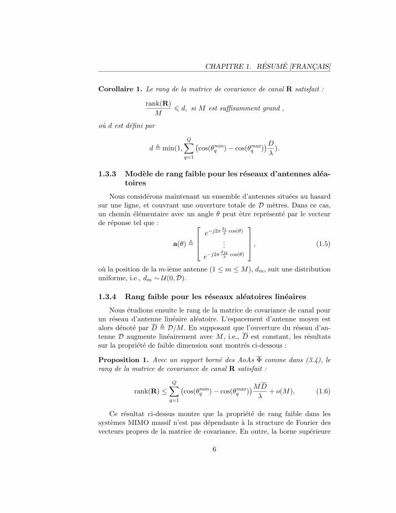
Corollaire 1. Le rang de la matrice de covariance de canal R satisfait :
rank(R)
M6 d, si M est suffisamment grand ,
ou d est defini par
d , min(1,
Q∑q=1
(cos(θmin
q )− cos(θmaxq )
)Dλ
).
1.3.3 Modele de rang faible pour les reseaux d’antennes alea-toires
Nous considerons maintenant un ensemble d’antennes situees au hasardsur une ligne, et couvrant une ouverture totale de D metres. Dans ce cas,un chemin elementaire avec un angle θ peut etre represente par le vecteurde reponse tel que :
a(θ) ,
e−j2π
d1λ
cos(θ)
...
e−j2πdMλ
cos(θ)
, (1.5)
ou la position de la m-ieme antenne (1 ≤ m ≤M), dm, suit une distributionuniforme, i.e., dm ∼ U(0,D).
1.3.4 Rang faible pour les reseaux aleatoires lineaires
Nous etudions ensuite le rang de la matrice de covariance de canal pourun reseau d’antenne lineaire aleatoire. L’espacement d’antenne moyen estalors denote par D , D/M . En supposant que l’ouverture du reseau d’an-tenne D augmente lineairement avec M , i.e., D est constant, les resultatssur la propriete de faible dimension sont montres ci-dessous :
Proposition 1. Avec un support borne des AoAs Φ comme dans (3.4), lerang de la matrice de covariance de canal R satisfait :
rank(R) ≤Q∑q=1
(cos(θmin
q )− cos(θmaxq )
)MD
λ+ o(M), (1.6)
Ce resultat ci-dessus montre que la propriete de rang faible dans lessystemes MIMO massif n’est pas dependante a la structure de Fourier desvecteurs propres de la matrice de covariance. En outre, la borne superieure
6
CHAPITRE 1. RESUME [FRANCAIS]
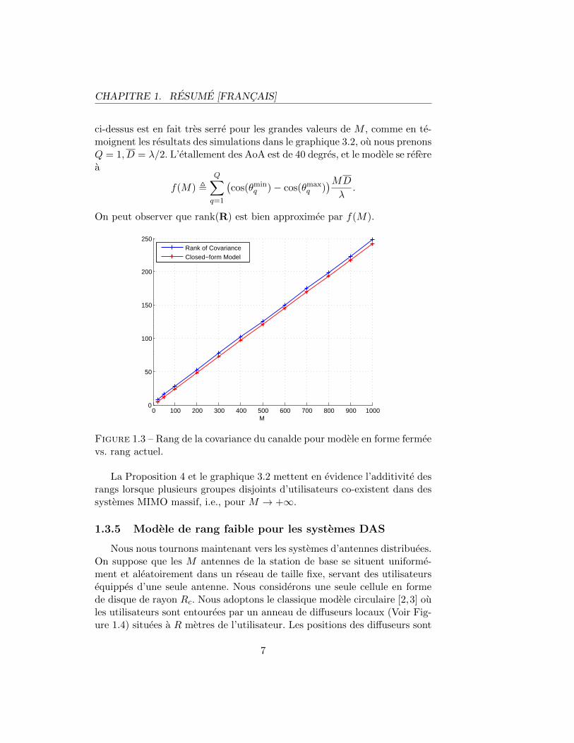
ci-dessus est en fait tres serre pour les grandes valeurs de M , comme en te-moignent les resultats des simulations dans le graphique 3.2, ou nous prenonsQ = 1, D = λ/2. L’etallement des AoA est de 40 degres, et le modele se referea
f(M) ,Q∑q=1
(cos(θmin
q )− cos(θmaxq )
)MD
λ.
On peut observer que rank(R) est bien approximee par f(M).
0 100 200 300 400 500 600 700 800 900 10000
50
100
150
200
250
M
Rank of CovarianceClosed−form Model
Figure 1.3 – Rang de la covariance du canalde pour modele en forme fermeevs. rang actuel.
La Proposition 4 et le graphique 3.2 mettent en evidence l’additivite desrangs lorsque plusieurs groupes disjoints d’utilisateurs co-existent dans dessystemes MIMO massif, i.e., pour M → +∞.
1.3.5 Modele de rang faible pour les systemes DAS
Nous nous tournons maintenant vers les systemes d’antennes distribuees.On suppose que les M antennes de la station de base se situent uniforme-ment et aleatoirement dans un reseau de taille fixe, servant des utilisateursequippes d’une seule antenne. Nous considerons une seule cellule en formede disque de rayon Rc. Nous adoptons le classique modele circulaire [2,3] oules utilisateurs sont entourees par un anneau de diffuseurs locaux (Voir Fig-ure 1.4) situees a R metres de l’utilisateur. Les positions des diffuseurs sont
7

CHAPITRE 1. RESUME [FRANCAIS]
BS antennas
MS 1
MS 2
Ring of Scatterers
r
Scatterers
Multipath
Figure 1.4 – Configuration distribuee dans le cadre d’une diffusion avecmodele circulaire.
consideres suivre une distribution uniforme sur l’anneau. De plus, chaquechemin de propagation rebondit une fois sur le diffuseur avant d’atteindretoutes les M destinations.
On considere ci-apres un reseau (dense) dans laquelle la perte de trajetest non negligeable.
Theoreme 2. Le rang de la matrice de covariance de canal pour un systemed’antenne distribues satisfait :
rank(R) ≤ 4πr
λ+ o(r). (1.7)
Le graphique3.4 montre le comportement du rang de la matrice de co-variance par rapport au rayon de diffusion r. Nous pouvons voir que le rangvarie lineairement avec la pente 4π/λ. Toutefois, en raison du nombre limited’antennes, le rang finit par saturer vers M quand r ne cesse d’augmenter.
1.3.6 Propriete de covariance uniformement bornee
Nous edutions maintenans comment borner la norme spectrale de la ma-trice de covariance du canal dans cadre d’un reseau d’antenne ULA. Cette
8

CHAPITRE 1. RESUME [FRANCAIS]
0 2 4 6 8 10 12 14 16 18 200
200
400
600
800
1000
1200
1400
1600
1800
r [m]
Rank of R4πr/λ
Figure 1.5 – Rank vs. r, M = 2000, λ = 0.15m, Rc = 500m.
propriete sera utile dans l’analyse du chapitre 5.
Proposition 2. Denotons par Φ le support des AoA sd’un certain utilisateuret par p(θ) la fonction de densite de probabilite de AoA de l’utilisateur. sip(θ) est est uniformement bornee, i.e., p(θ) < +∞,∀θ ∈ Φ, et Φ se situedans un intervalle ferme qui ne comprend pas les directions paralleles parrapport a la matrice, i.e., 0, π /∈ Φ, alors, la norme spectrale de covariancede l’utilisateur R est uniformement bornee :
∀M, ‖R‖2 < +∞. (1.8)
1.3.7 Conclusions
Dans cette section, nous soulignons plusieurs proprietes fondamentalesdes chaınes des utilisateurs de MIMO massifs. Nous etudions les proprietes decovariance de sous-espaces de signaux en basse dimension dans des topologiesgenerales de massifss array,y compris array uniforme lineaire, array lineairealeatoire, et array distribuee en 2D.Une autre propriete revele est le bor-nitude uniforme de la norme spectrale de covariance de canal pour ULA.Ces proprietes seront utiles dans les sections suivantes pour reduire les in-terferences et pour reduire la quantite de feedback CSI.
9

CHAPITRE 1. RESUME [FRANCAIS]
1.4 Estimation de canal basee sur la covariance
Dans cette section, nous exploitons le rang faible de la matrice de covari-ance afin de faciliter l’acquisition de l’information de canal dans les systemesMIMO massif, dans le cadre d’un fonctionnement en TDD. Nous proposonsune methode d’estimation conduisant a une amelioration considerable de laperformance. En particulier, nous mettons en evidence que la connaissancede la matrice de covariance peut conduire a une elimination complete deseffets de la contamination de pilote dans la limite d’un grand nombre d’an-tennes a la station de base. Un algorithme permettant l’exploitation de ceconcepte dans des scenarios pratiques est ensuite presente. L’idee principaleest d’utiliser la connaissance des matrices de covariance lors de l’affectationdes pilotes d’estimation du canal.
1.4.1 Apprentissage du canal pour la connection montante
Pour faciliter la comprehension, nous considerons dans le reste de lasection qu’un seul utilisateur par cellule est present. La suite de pilotesutilisee dans la l-ieme cellule est denotee par :
s` = [ s`1 sl2 · · · s`τ ]T . (1.9)
Les puissances allouees aux sequences de pilotes sont supposees egales detelle sorte que |sl1|2+· · ·+|slτ |2 = τ, l = 1, 2, . . . , L. Sans perte de generalite,nous supposons que la premiere cellule est la cellule cible de telle sorte quenous puissions omettre l’exposant du canal. Le canal entre l’utilisateur de la`-ieme cellule et la station de base cible est donc denote par h`.
Lors de la transmission des pilotes, le signal M × τ recu a la station debase cible est donc
Y =L∑l=1
hlsTl + N, (1.10)
ou N ∈ CM×τ est le bruit blanc additif Gaussien, centre et de variance σ2n.
1.4.2 Estimation bayesienne du canal
Par la suite, nous developpons des estimateurs de canal se basant surles statistiques de second ordre des canaux. Deux estimateurs bayesiens decanal peuvent ainsi etre construits. Dans un premier temps, tous les canauxsont estimes a la station de base cible (y compris les interferents). Dans lesecond temps, seulement h1 est estime.
10

CHAPITRE 1. RESUME [FRANCAIS]
En representation vectorielle, notre modele (5.3) peut etre representecomme
y = Sh + n, (1.11)
ou y = vec(Y), n = vec(N), and h ∈ CLM×1 est obtenu en ecrivant suc-cessivement les L canaux. La matrice des pilotes, denotee par S, est ainsidefinie par
S ,[
s1 ⊗ IM · · · sL ⊗ IM]. (1.12)
Utilisant la methode du maximum a posteriori (MAP), l’estimation bayesi-enne est donnee par :
h = (σ2nILM + RSH S)−1RSHy. (1.13)
Il est remarquable que l’estimation bayesienne dans (4.13) coıncide avecl’erreur quadratique moyenne minimum (MMSE) lorsque le canal h suit ladistribution gaussienne complexe.
Considerons le scenario pessimiste ou une seule sequence de pilotes estutilisee dans les L cellules et representee par
s = [ s1 s2 · · · sτ ]T . (1.14)
Nous definissons ensuite la matrice d’apprentissage S , s⊗ IM . Il s’ensuitealors que SH S = τIM . Le signal vectorise d’apprentissage recue a la stationde base cible peut donc etre exprime comme
y = S
L∑l=1
hl + n. (1.15)
L’estimateur bayesien (equivalent a l’estimateur MMSE) pour le canal spe-cifique h1 est ainsi represente par :
h1 = R1SH
(S
(L∑l=1
Rl
)SH + σ2
nIτM
)−1
y (1.16)
= R1
(σ2nIM + τ
L∑l=1
Rl
)−1
SHy. (1.17)
Dans la section ci-dessous, nous examinons la degradation causee par lacontamination de pilote sur la qualite de l’estimation.
11

CHAPITRE 1. RESUME [FRANCAIS]
Analyse a grande echelle
Nous cherchons a analyser la performance des estimateurs ci-dessus dansle regime d’un grand nombre d’antennes M . Afin d’obtenir des resultatsanalytiques, notre analyse est basee sur l’hypothese d’ULA.
Theoreme 3. Supposons que l’angle arrivee θ des trajets multiples du canalhj , j = 1, . . . , L, est distribue selon une densite arbitraire pj(θ) ayant unsupport borne, i.e., pj(θ) = 0, θ /∈ [θmin
j , θmaxj ], pour θmin
j 6 θmaxj ∈ [0, π] .
Si les L − 1 intervalles [θmini , θmax
i ] , i = 2, . . . , L sont strictement distinctsdu support de l’angle d’arrive du canal direct 1 [θmin
1 , θmax1 ], on a
limM→∞
h1 = hno int1 . (1.18)
0 20 40 60 80 100 120 140 160 180 200−40
−35
−30
−25
−20
−15
−10
Number of Antennas
Est
imat
ion
Err
or [d
B]
Conventional LS EstimationCovariance−aided Bayesian (CB) Estimation LS − Interference Free ScenarioCB − Interference Free Scenario
Figure 1.6 – Estimation MSE vs. nombre BS antennes , 2-cellule net-work, deux utilisateurs en position fixee, AOA uniformement distribueesavec θ∆ = 20 degres, nans chevauchement trajets multiples.
1. Cette condition correspond simplement a un scenario pratique conduisant a dessous-espaces de signaux distincts entre la matrice de covariance souhaitee et la matricede covariance des interferences. Cependant, des scenarios plus generaux pourraient etreutilises.
12

CHAPITRE 1. RESUME [FRANCAIS]
Les resultats presentes dans le Theoreme 3 sont verifies numeriquementdans Le graphique4.1 dans le cas d’un reseau compose de deux cellules etou les positions de deux utilisateurs sont fixees. Les angles d’arrivees ducanal direct sont uniformement distribuees avec une moyenne egale a 90degres et avec un etalement angulaire egale a 20 degres, ce qui donne pasde chevauchement entre les multi-trajets souhaites et celui de l’interference.Comme on le voit, l’erreur d’estimation de canal converge vers le cas sansinterference, ce qui indique que la contamination des pilotes est elimineeavec le nombre d’antennes en croissant.
Theoreme 3 donne la condition suffisante pour atteindre la suppressiontotale de l’interference lorsque M est grand :
L∪l=2
span {Rl} ⊂ null {R1} (1.19)
ou la condition ci-dessus necessite que la matrice de covariance du canaldesire aie un noyau non-vide et que les sous-espaces engendres par les ma-trices de covariance de toutes les interferences tombent dans ce noyau.
Le Theoreme 3 est limite au cas ou le support de l’angle d’arrive du canaldirect est un unique interval. Nous allons donner ci-dessous les resultatsetendus dans des conditions moins restrictives.
Cas de plusieurs groupe d’angles d’arrive
Nous considerons maintenant le modele general de propagation par tra-jets multiples lorsque les angles d’arrive du canal d’un certain utilisateursont limitees, mais proviennent de plusieurs groupes disjoints, comme decritdans la Section 1.3.2. Soit Φd l’union des angles d’arrives possibles du canaldirect et Φi l’union des angles d’arrive de l’interference. Nous avons le re-sultat suivant pour le cas d’un reseau d’antenne uniforme massif :
Corollaire 2. Soit D ≤ λ/2 and Φd ∩ Φi = ∅. L’estimation MMSE pour(1.17) satisfait :
limM→∞
h1 = hno int1 . (1.20)
1.4.3 Affectation coordonnee des pilotes
Dans cette section, nous concevons un protocole de coordination perme-ttant de distribuer les sequences de pilotes aux utilisateurs. Le role de lacoordination est d’optimiser l’utilisation des matrices de covariance dans lebut de satisfaire la condition de non chevauchement des supports des angles
13
CHAPITRE 1. RESUME [FRANCAIS]
d’arrive. Nous utilisons l’estimation de MMSE comme metrique de perfor-mance afin de trouver le meilleur groupe d’utilisateur. Le principe de ladistribution des pilotes coordonnee consiste a exploiter la connaissance desmatrices de covariance.
Nous proposons une approche gloutonne/gourmande classique appeleAffectation Coordonnee des Pilotes (CPA). La coordination peut etre in-terpretee comme suit : Pour minimiser l’erreur d’estimation, une station debase tend a affecter un pilote donne a l’utilisateur dont la caracteristiquespatiale differe fortement avec les utilisateurs interferents utilisant le memepilote.
Deux types de distributions de l’angle d’arrive sont considerees ici, unnon-borne (Gaussien) et un borne (uniforme) :
Distribution Gaussienne
Pour certain canal h(j)`k , les angles d’arrive pour tous les trajets P sont
i.i.d. Gaussiennes de moyenne θ(j)`k et de variance σ2.
Notez que les distributions Gaussienne des angles d’arrive ne peuventpas satifaire les conditions de non chevauchement des supports des anglesd’arrive du Theoreme 3, neanmoins l’utilisation de la methode proposee dansce contexte donne egalement des gains substantiels lorsque σ2 diminue.
Distribution uniforme
Pour les canaux h(j)`k , les angles d’arrive sont uniformement reparties sur
[θ(j)lk − θ∆, θ
(j)lk + θ∆], ou θ
(j)`k est la moyenne des angles d’arrive.
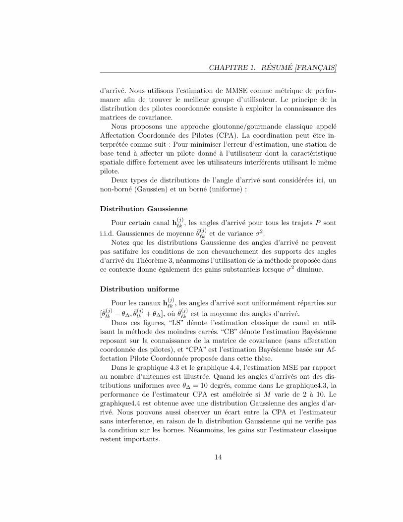
Dans ces figures, “LS” denote l’estimation classique de canal en util-isant la methode des moindres carres. “CB” denote l’estimation Bayesiennereposant sur la connaissance de la matrice de covariance (sans affectationcoordonnee des pilotes), et “CPA” est l’estimation Bayesienne basee sur Af-fectation Pilote Coordonnee proposee dans cette these.
Dans le graphique 4.3 et le graphique 4.4, l’estimation MSE par rapportau nombre d’antennes est illustree. Quand les angles d’arrives ont des dis-tributions uniformes avec θ∆ = 10 degres, comme dans Le graphique4.3, laperformance de l’estimateur CPA est ameloiree si M varie de 2 a 10. Legraphique4.4 est obtenue avec une distribution Gaussienne des angles d’ar-rive. Nous pouvons aussi observer un ecart entre la CPA et l’estimateursans interference, en raison de la distribution Gaussienne qui ne verifie pasla condition sur les bornes. Neanmoins, les gains sur l’estimateur classiquerestent importants.
14

CHAPITRE 1. RESUME [FRANCAIS]
0 5 10 15 20 25 30 35 40 45 50−40
−35
−30
−25
−20
−15
−10
−5
Number of Antennas
Est
imat
ion
Err
or [d
B]
Conventional LS EstimationCovariance−aided Bayesian EstimationCoordinated Pilot Assignment−based EstimationLS − Interference Free ScenarioCB − Interference Free Scenario
Figure 1.7 – Estimation MSE vs. nombre de BS antennes, AOA uniforme-ment distribuees avec θ∆ = 10 degres, 2-cellules network.
0 5 10 15 20 25 30 35 40 45 50−40
−35
−30
−25
−20
−15
−10
−5
Number of Antennas
Est
imat
ion
Err
or [d
B]
LS Estimation
CB Estimation
CPA Estimation
LS − Interference Free
CB − Interference Free
Figure 1.8 – Estimation MSE vs. number of BS antennas, AOA distribuesgaussienne σ = 10 degrees, 2-cell network.
15

CHAPITRE 1. RESUME [FRANCAIS]
0 5 10 15 20 25 30 35 40 45 504
6
8
10
12
14
16
18
Number of Antennas
Per
−ce
ll R
ate
[bits
/sec
/Hz]
Conventional LS EstimationCovariance−aided Bayesian EstimationCoordinated Pilot Assignment−based Estimation
Figure 1.9 – Taux par cellule vs. nombre de BS antennes, 2-cellules network,AOA distribues gaussienne avec σ = 10 degres.
Le graphique4.6 decrit le debit de la connection descendante pour unecellule, obtenu par la strategie de precodage adapte et comfirme les gainsobtenus lorsque l’estimation Bayesienne est utilise en conjonction avec lastrategie d’affectation coordonnee des pilotes (CPA) proposee et des gainsintermediaires quand il est utilise tout seul.
1.4.4 Conclusions
Cette partie propose une metode d’estimation du canal se basant surla connaissance de la matrice de covariance dans le contexte de systemesmulti-cellulaires et d’antennes multiples dans le cas d’un regime limite parles interferences. Nous developpons des estimateurs Bayesiens et demontronsanalytiquement l’efficacite d’une telle approche pour les systemes ayant ungrand nombre d’antennes, conduisant a une elimination complete des ef-fets de la contamination de pilote dans le cas de matrices de covariancesatisfaisant une certaine condition de non-chevauchement des supports desangles d’arrive. Nous proposons une strategie d’affectation coordonnee despilotes (CPA) qui aide a former des matrices de covariance verifiant la con-dition necessaire et mettons en evidence que des performances proches del’estimation sans interference peuvent etre atteintes.
16

CHAPITRE 1. RESUME [FRANCAIS]
1.5 Decontamination basee sur la puissance et lesangles
Dans la section precedente, nous avons montre plusieurs techniques d’at-tenuation des interferences se basant sur la connaissance statistique descanaux des utilisateurs. Plus particulierement, nous avons demontre quedans le cas ou le support des angles d’arrive du canal direct ne se chevauchepas avec le support des angles d’arrives des utilisateurs interferents, unemethode basee sur l’estimation MMSE atteint l’elimination totale des inter-ferences. Cependant, quand une telle condition de non-chevauchement n’estpas satisfaite, une interference residuelle existe lors de l’estimation MMSE,ce qui limite la performance des systeme MIMO massif. Dans cette section,nous cherchons a resoudre ce type de probleme en exploitant les statistiquesa court terme du canal.
1.5.1 Transmission de donnees
Soit un reseau multi-cellules multi-utilisateur ayant K utilisateurs parcellule, et chacun desservi par sa propre station de base. Le canal multi-utilisateur MIMO entre les K utilisateurs dans la cellule ` et la station debase j est :
H(j)` ,
[h
(j)`1 h
(j)`2 · · · h
(j)`K
], (1.21)
et la matrice des pilote se composant de toutes les sequences de pilotesutilises par ces K utilisateurs est :
S ,[s1 s2 · · · sK
]T. (1.22)
Pendant la phase d’apprentissage, le signal recu a la station de base j est
Y(j) =L∑`=1
H(j)` S + N(j), (1.23)
ou N(j) ∈ CM×τ est le spatialement et temporellement blanc bruit gaussienadditif (AWGN) avec moyenne nulle et variance element par element σ2
n.Ensuite, pendant la phase de transmission de donnees de liaison mon-
tante, chaque utilisateur transmet C symboles de donnees. Le signal de don-nees recu a la station de base j est donne par :
W(j) =
L∑`=1
H(j)` X` + Z(j), (1.24)
17

CHAPITRE 1. RESUME [FRANCAIS]
ou X` ∈ CK×C est la matrice de symboles emis par tous les utilisateursdans la `-ieme cellule. Les symboles sont i.i.d. avec une moyenne nulle etune variance unitaire. La matrice Z(j) ∈ CM×C a ses elements i.i.d Gaussienavec moyenne nulle et variance σ2
n.
1.5.2 Methode basee sur la projection dans le domaine del’amplitude
Nous proposons ci-dessous de nouvelles methodes d’estimation permet-tant une estimation plus robust dans un scenario cellulaire realiste.
Un seul utilisateur par cellule
Par soucis de clarete, nous considerons d’abord un scenario simple ouchaque cellule a un seul utilisateur, a savoir K = 1. Les utilisateurs dans descellules differentes partagent la meme sequence de pilote s.
On introduit un filtre Ξj , qui est base sur la connaissance des matricesde covariance de canal d’une maniere similaire a celle utilisee par le filtreMMSE.
Ξj =
(L∑l=1
R(j)l + σ2
nIM
)−1
R(j)j . (1.25)
Le filtre spatial est applique au signal recu a la station de base j comme
Wj , ΞjW(j). (1.26)
La methode basee sur l’amplitude peut maintenant etre applique sur les don-nees recues filtrees pour se debarrasser de l’interference residuelle. Prendrele vecteur propre correspondant a la plus grande valeur propre de la matriceWjW
Hj /C :
uj1 = e1{1
CWjW
Hj }. (1.27)
Donc uj1 peut etre consideree comme une estimation de la direction du
vecteur Ξjh(j)j .
Nous annulons alors l’effet de la multiplication par la matrice Ξj enutilisant
Ξj′ , R
(j)†
j
(L∑l=1
R(j)l + σ2
nIM
), (1.28)
18

CHAPITRE 1. RESUME [FRANCAIS]
et on obtient une estimation de la direction du vecteur de canal h(j)j comme
la suite :
uj1 =Ξ′juj1∥∥∥Ξ′juj1∥∥∥
2
. (1.29)
Enfin, les ambiguıtes de phase et d’amplitude du canal peuvent etre resoluspar la projection de l’estimation selon la methode des moindres carres surle sous-espace engendre par uj1 :
h(j)CAj =
1
τuj1u
Hj1Y
(j)s∗, (1.30)
ou “CA” designe la projection dans le domaine d’amplitude en covariance.
L’algorithme est resume ci-dessous :
Algorithm 1 Covariance-aided Amplitude based Projection
1: Prenez le premier vecteur propre de WjWHj /C comme dans (1.27), avec
Wj etant le signal de donnees filtre.2: Inverser l’effet du filtre spatial utilisant(1.29).3: Resoudre les ambiguıtes de phase et d’amplitude par(1.30).
Les performances asymptotique de l’estimateur ci-dessus sont analyseestheoriquement. Afin de faciliter l’analyse, nous introduisons la conditionsuivante :
Condition C1 : La norme spectrale de R(j)l est uniformement bornee :
∀M ∈ Z+ et∀l ∈ {1, . . . , L}, ∃ζ, s.t.∥∥∥R(j)
l
∥∥∥2< ζ, (1.31)
ou Z+ est l’ensemble des nombres entiers positifs, et ζ est une constante.
Performance asymptotique de l’estimateur CA
Soit
α(j)l , lim
M→∞
1
Mtr{ΞjR
(j)l ΞH
j },∀l = 1, . . . , L. (1.32)
Theoreme 4. Compte tenu de la condition C1, si l’inegalite suivante estvraie :
α(j)j > α
(j)l ,∀l 6= j, (1.33)
19

CHAPITRE 1. RESUME [FRANCAIS]
0 50 100 150 200 250 300 350 400 450 500−20
−15
−10
−5
0
5
Number of Antennas
Est
imat
ion
Err
or [d
B]
LS estimationPure MMSEPure amplitudeMMSE + amplitudeCovariance−aided amplitudeMMSE − no interference
Figure 1.10 – Estimation des performance versus M pour un reseau a deux-cellules avec un utilisateur par cellule, un exposant d’attenuation γ = 0 etun support angulaire recouvrant partiellement les angles d’arrives a hauteurde 60 degres, C = 500, SNR = 0 dB.
alors, l’erreur d’estimation de (1.30) disparaıt :
limM,C→∞
∥∥∥h(j)CAj − h
(j)j
∥∥∥2
2∥∥∥h(j)j
∥∥∥2
2
= 0. (1.34)
De plus, la condition (1.33) du Theoreme 4 peut alors etre remplace par∥∥∥Ξjh(j)j
∥∥∥2>∥∥∥Ξjh
(j)l
∥∥∥2, ∀l 6= j. (1.35)
Nous illustrons maintenant le Theoreme 4 dans le graphique 5.1. Supposonsqu’on aie un reseau compose de deux cellules et que chaque cellule aie deuxutilisateurs. L’exposant d’attenuation est γ = 0, i.e., la puissance de l’inter-ference de canal est la meme que celle du canal direct. Les supports angu-laires a trajets multiples de l’interference et le canal desire se superposentdonc a hauteur de 50 Dans cette courbe, “Pure amplitude” denote la meth-ode de projection basee seulement sur l’amplitude. “MMSE + amplitude”represente l’estimateur a faible complexite propose dans [4]. “Covariance-aided amplitude” denote la methode de projection utilisant l’amplitude et
20

CHAPITRE 1. RESUME [FRANCAIS]
0 50 100 150 200 250 300 350 400 450 500−25
−20
−15
−10
−5
0
5
Number of Antennas
Est
imat
ion
Err
or [d
B]
LS estimationPure MMSEPure amplitudeMMSE + amplitudeCovariance−aided amplitude
Figure 1.11 – Estimation performance vs. M, 7-cellules network, 1 utilisa-teurs par cellule, AoA reparties 60 degres, exposant de perte de trajet γ = 2,cellule-bord SNR = 0 dB.
la connaisance de la matrice de covariance (1.30). La courbe “MMSE - nointerference” montre l’erreur d’estimation de l’estimateur MMSE dans unscenario sans interference et sert ainsi de reference. Comme on peut le voirsur la courbe 5.1, la methode de projection utlisant l’amplitude et la covari-ance surpasse la methode d’estimation MMSE sans interferences.
Dans la courbe 5.2, nous considerons un reseau compose de 7 cellules,avec un seul utilisateur par cellule. Les utilisateurs sont supposes etre dis-tribues de facon aleatoire et uniforme au sein de leurs propres cellules. Lapropagation angulaire du canal d’utilisateur est de 30 degres. L’exposantd’attenuation est fixe a γ = 2. Il est possible d’observer comment la meth-ode de projection exploitant a la fois la connaissance de l’amplitude et de lamatrice de covariance est plus performante que les autres methodes.
Generalisation a plusieurs utilisateurs par cellule
Nous appliquons maintenant la methode de projection base sur l’ampli-tude et la connaissance de la matrice de covariance dans le cas general, c’esta dire lorsque K utilisateurs sont servis simultanement dans chaque cellule.
Nous considerons l’estimation du canal d’utilisateur h(j)jk dans la suite de
cette section.
21

CHAPITRE 1. RESUME [FRANCAIS]
Pour simplifier les notations, nous introduisons la notation H(j)j\k pour
representer H(j)j apres avoir enleve sa k-ieme colonne :
H(j)j\k ,
[h
(j)j1 · · · h
(j)j(k−1) h
(j)j(k+1) · · · h
(j)jK
]. (1.36)
L’estimation correspondant a (1.36), denotee par H(j)j\k, est obtenue en elim-
inant la k-ieme colonne de H(j)j , qui est une estimation selon la methode des
moindre carres de H(j)j .
Nous neutralisons tout d’abord l’interference intra-cellulaire avec un fil-tre dit de Zero-Forcage (ZF) et denote par Tjk en utilisant l’estimee H
(j)j\k.
Ensuite, le filtre spatial Ξjk est appliquee. A l’issue de l’application de ces2 filtres, le signal obtanu est :
Wjk , ΞjkTjkW(j), (1.37)
ou
Tjk , IM − H(j)j\k(H
(j)Hj\k H
(j)j\k)
−1H(j)Hj\k , (1.38)
et
Ξjk ,
(L∑l=1
R(j)lk + σ2
nIM
)−1
R(j)jk . (1.39)
Hormis ces modifications, la methode decrite dans le cas d’un seul utilisateurpeut etre appliquee.
Soit le vecteur propre correspondant a la plus grande valeur propre dela matrice WjkW
Hjk/C :
ujk1 = e1{1
CWjkW
Hjk}. (1.40)
L’estimation de la direction de h(j)jk est obtenue par :
ujk1 =Ξ′jkujk1∥∥∥Ξ′jkujk1
∥∥∥2
, (1.41)
ou
Ξ′jk , R(j)†jk
(L∑l=1
R(j)lk + σ2
nIM
). (1.42)
22
CHAPITRE 1. RESUME [FRANCAIS]
Enfin, les ambiguıtes de phase et d’amplitude sont resolu durant la sequence
d’apprentissage pour obtenir l’estimation de h(j)jk :
h(j)CAjk =
1
τujk1u
Hjk1Y
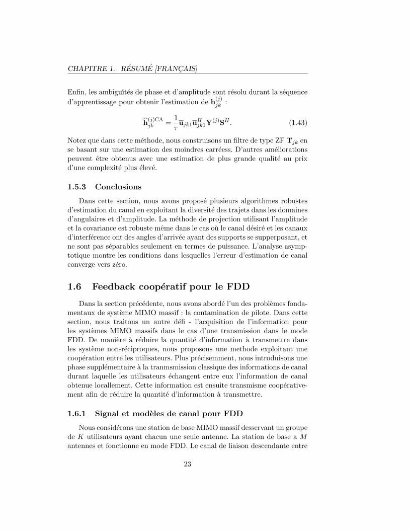
(j)SH . (1.43)
Notez que dans cette methode, nous construisons un filtre de type ZF Tjk ense basant sur une estimation des moindres carreess. D’autres ameliorationspeuvent etre obtenus avec une estimation de plus grande qualite au prixd’une complexite plus eleve.
1.5.3 Conclusions
Dans cette section, nous avons propose plusieurs algorithmes robustesd’estimation du canal en exploitant la diversite des trajets dans les domainesd’angulaires et d’amplitude. La methode de projection utilisant l’amplitudeet la covariance est robuste meme dans le cas ou le canal desire et les canauxd’interference ont des angles d’arrivee ayant des supports se supperposant, etne sont pas separables seulement en termes de puissance. L’analyse asymp-totique montre les conditions dans lesquelles l’erreur d’estimation de canalconverge vers zero.
1.6 Feedback cooperatif pour le FDD
Dans la section precedente, nous avons aborde l’un des problemes fonda-mentaux de systeme MIMO massif : la contamination de pilote. Dans cettesection, nous traitons un autre defi - l’acquisition de l’information pourles systemes MIMO massifs dans le cas d’une transmission dans le modeFDD. De maniere a reduire la quantite d’information a transmettre dansles systeme non-reciproques, nous proposons une methode exploitant unecooperation entre les utilisateurs. Plus precisemment, nous introduisons unephase supplementaire a la tranmsmission classique des informations de canaldurant laquelle les utilisateurs echangent entre eux l’information de canalobtenue locallement. Cette information est ensuite transmisme cooperative-ment afin de reduire la quantite d’information a transmettre.
1.6.1 Signal et modeles de canal pour FDD
Nous considerons une station de base MIMO massif desservant un groupede K utilisateurs ayant chacun une seule antenne. La station de base a Mantennes et fonctionne en mode FDD. Le canal de liaison descendante entre
23

CHAPITRE 1. RESUME [FRANCAIS]
la station de base et l’utilisateur k est note hHk ∈ C1×M . Le canal de liaisondescendante entier peut donc etre represente par
HH =
hH1...
hHK
∈CK×M
. (1.44)
La transmission de liaison descendante est modelisee par :
y = HHBs + n, (1.45)
ou y ∈ CK×1 est le signal recu par tous les utilisateurs, s ∈ CK×1 representele vecteur de signaux Gaussiens i.i.d., et n represente le bruit blanc Gaussien,centre, et une variance egale a σ2
n. B est la formation de faisceau de liaisondescendante ayant la puissance totale P .
Nous considerons un scenario dans lequel K utilisateurs sont situes aproximite les uns des autres de telle sorte que leurs canaux presentent lesmeme caractistiques statistiques, i.e., ∀k,E{hkhHk } = R. Le rang de R estsuppose etre egale a d. Soit la decomposition en valeur propres (EVD) deR :
R = UΣUH (1.46)
En supposant que les valeurs propres de Σ sont triees par ordre decroissant,les d premieres colonnes de U sont extraites pour former une sous-matriceU1 ∈ CM×d. Le vecteur de canal hk est donc dans l’espace engendre par U1,c’est-a-dire ∀k,hk est une combinaison lineaire des colonnes de U1.
H =[h1 h2 · · · hk
]= U1A, (1.47)
ou A∈ Cd×K est defini comme :
A ,[a1 a2 · · · aK
]=
a11 a12 · · · a1K
a21 a22 · · · a2K...
... · · ·...
ad1 ad2 · · · adK
. (1.48)
1.6.2 Conception de l’acquisition de l’information de canalsans D2D
La strategie traditionnelle de feedback pour les systeme multi-utilisateursest de laisser chaque utilisateur quantifier son vecteur de canal de liaison de-scendante puis envoyer l’information quantifiee a la station de base [5]. A
24

CHAPITRE 1. RESUME [FRANCAIS]
noter que dans la configuration MIMO massif, seulement une part de l’in-formation de canal (notamment K coefficients par utilisateur) est necessairepour atteindre l’orthogonalite entre les signaux de l’utilisateur.
En extrayant N lignes avec K ≤ N ≤ d de la matrice A, on peux obtenirune matrice As∈ CN×K ; En prenant N colonnes correspondantes de U1,on obtaient ainsi la matrice Us∈ CM×N . Nous pouvons alors reconstruirepartiellement la matrice de canal de la maniere suivante :
H , UsAs. (1.49)
Un filtre ZF utilisant cette information de canal peut alors etre ecrit comme
B =
√P H†
||H†||F. (1.50)
Il est decrit dans [6] comment former la matrice As en extrayant lineaire-ment arbitrairement une sous-matrice de taille K × d de A. Si la station debase connait obtient cette information de canal incomplete, elle garantit queles utilisateurs ne recoivent pas d’interferences apres application du filtrageZF (1.50). Lorsque l’echange d’information de canal entre les utilisateursn’est pas possible, il est raisonnable de choisir les vecteurs propres des pre-miers K lignes depuis U1 dans la mesure ou ils representent les K vecteurspropres les plus forts en terme de statistiques.
1.6.3 Acquisistion cooperative de l’information de canal avecD2D
Lorsque l’echange de l’information de canal est rendue possible entre lesutilisateurs, ceux-ci peuvent prendre une decision conjointe et determinerconjointement quel ensemble de vecteurs propres de U1, ou egalement quelslignes extraire de A pour former la matrice As. Par exemple, nous pouvonsconsiderer le SNR a cote de l’utilisateur comme critere :
SNR =P
||H†||2F=
P
tr{(AHs As)−1}
. (1.51)
Nous choisissons alors K parmi les d vecteurs propres de U1 pour que leSNR soit maximisee.
G(2) = argN=K
min tr{(AHs As)
−1}. (1.52)
L’optimalite de la decision de selection des vecteurs propres est atteintepar un algorithme de selection decrementielle qui est explique dans [7] [8].
25

CHAPITRE 1. RESUME [FRANCAIS]
Nous commencons par considere le canal effectif A dans sa totalite. Sous lacondition que le SNR est minimum, les lignes de A sont retires un par un,jusqu’a il reste K lignes.
Lorsque la decision conjointe est prise, i.e., pour G(2), les utilisateurstransmettent alors a la station de base la matrice As (quantifie) correspon-dante, ainsi que les indices de G(2).
Trois regimes differents d’acquisition de l’information de canal sont eval-ues et les performances des debits totaux sont donnes dans la Figure 6.1.
0 5 10 15 20 25 300
5
10
15
20
25
Cell edge SNR [dB]
Sum
−ra
te [b
ps]
Use strongest K eigen modes, no D2DQuantize full CSI, no D2DCooperative feedback of CSI, D2D
16 bits feedbackper user
Figure 1.12 – DL sum-rates with/without feedback cooperation, feedbackoverhead : 16 bits per user, K = 3, M = 50.
Pour comparison, on suppose que la meme quantite de bits de quan-tification est disponible dans chacun des trois regimes. Chaque utilisateurtransmet alors 16 bits d’information a la station de base. La courbe“Quantizefull CSI, no D2D”designe la performance lorsque la matrice de canal effectiveA est transmie dans sa totalite. La courbe “Use strongest K eigen modes,no D2D” indique la performance de chaque utilisateur pour K vecteurs pro-pres dominants de R. La courbe “Cooperative feedback of CSI, D2D” faitreference a la nouvelle methode proposee. Les utilisateurs transmettent alorsles projections quantifiees et les indices des trois vecteurs propres qui sontchoisis. Les simulations numeriques mettent clairement en evidence le gain
26

CHAPITRE 1. RESUME [FRANCAIS]
de la methode proposee.
1.6.4 Acquisition cooperative de l’indice du precodeur avecD2D
Nous considerons maintenant une autre approche dans laquelle l’infor-mation de canal n’est pas explicitement transmise mais l’indice du precodeura utiliser est transmis. L’echange de l’information de canal via D2D commu-nications entre les utilisateurs permet a ceux-ci de choisir conjointement unematrice de precodage. Apres l’echange de cette information, les utilisateursselectionnent conjointement la meilleure matrice de precodage selon un cer-tain critere, et transmettent l’indice de la matrice de precodage selectionnee.Le critere de selection peut varier en fonction de l’exigence de la complexitedu systeme. Un choix intuitive est la maximisation du debit total C.
Pour clarifier cette description, les principales etapes sont rappelees dansla suite :
(1) Les utilisateurs envoient leur information de canal a un certain util-isateur ”maıtre”. Cet utilisateur maıtre a maintenant la matrice effective decanal A.
(2) L’utilisateur maıtre recherche dans le dictionnaire l’indice du pre-codage qui maximise le debit total :
(3) L’utisateur maıtre transmet cet indice a la station de base.
(4) La station de base effectue un filtrage en utilisant la matrice dudictionnaire designee par l’indice recu.
Les performances atteintes en utilisant cette methodes sont illustreesnumeriquement dans le graphique 6.2. Comme on peut le voir, la methodeproposee apporte de significatifs gains de performance.
1.6.5 Conclusions
Dans cette section, nous proposons nue nouvelle methode permettantl’acquisition de l’information de canal lorsque les transmission s’effectuenten mode FDD. Cette methode repose sur l’echange d’information de canalentre les utilisateurs de maniere a optimiser la transmission vers la station debase. Deux approches sont proposees pour l’optimisation de la transmissionvers la station de base apres l’etape de partage de l’information. Dans lapremiere, l’information de canal est expicitement transmise alors que dansla deuxieme c’est l’indice du filtre a utiliser qui est transmis. Ces methodesaident a reduire le cout de l’acquisition de l’information de canal dans dessystemes FDD MIMO massif.
27

CHAPITRE 1. RESUME [FRANCAIS]
0 5 10 15 20 25 300
1
2
3
4
5
6
7
8
9
10
Cell edge SNR [dB]
Sum
−ra
te [b
ps]
Use strongest K eigen modes, no D2D
Quantize full CSI, no D2D
Cooperative feedback of precoder index, D2D
4 bits feedbackper user
Figure 1.13 – DL Sum-taux de selection cooperative de pre-codage et non-cooperative CSI feedback, feedback overhead : 4 bits par utilisateur.
1.7 Publications
Les publications suivantes sont le resultat des travaux realises au coursdu doctorat.
1.7.1 Conferences
1. Haifan Yin, David Gesbert, Miltiades Filippou, and Yingzhuang Liu“Decontaminating pilots in MIMO massifs systems”, International Con-ference on Communications (ICC 2013), Jun. 9-13, 2013, Budapest,Hungary.
2. Miltiades Filippou, David Gesbert, and Haifan Yin,“Decontaminatingpilots in cognitive MIMO massifs networks,” 9th IEEE InternationalSymposium on Wireless Communications Systems (ISWCS 2012), Aug.28-31, 2012, Paris, France (invited).
3. Haifan Yin, David Gesbert, and Laura Cottatellucci “A statistical
28

CHAPITRE 1. RESUME [FRANCAIS]
approach to interference reduction in distributed large-scale antennasystems”, International Conference on Acoustics, Speech and SignalProcessing (ICASSP 2014), May, 2014, Florence, Italy.
4. Haifan Yin, Laura Cottatellucci, and David Gesbert,“Enabling MIMOmassifs systems in the FDD mode thanks to D2D communications”,Asilomar Conference on Signals, Systems, and Computers (Asilomar2014), Nov. 2-5, 2014, Pacific Grove, CA, USA (invited),
5. Haifan Yin, Laura Cottatellucci, David Gesbert, Ralf R. Muller, andGaoning He, “Pilot decontamination using combined angular and am-plitude based projections in MIMO massifs systems”, IEEE 16th Work-shop on Signal Processing Advances in Wireless Communications (SPAWC2015), Jun. 28 - Jul. 1, 2015, Stockholm, Sweden. (invited).
6. Junting Chen, Haifan Yin, Laura Cottatellucci, and David Gesbert,“Precoder feedback versus channel feedback in MIMO massifs underuser cooperation,” 49th Asilomar Conference on Signals, Systems, andComputers (Asilomar 2015), Nov. 8-11, 2015, Pacific Grove, CA, USA(invited).
7. Haifan Yin, Laura Cottatellucci, David Gesbert, Ralf R. Muller, andGaoning He, “Robust pilot decontamination : A joint angle and powerdomain approach”, International Conference on Acoustics, Speech andSignal Processing (ICASSP 2016), Mar. 20 - Mar. 25, 2016, Shanghai,China.
1.7.2 Journaux
1. Haifan Yin, David Gesbert, Miltiades Filippou, and Yingzhuang Liu“A coordinated approach to channel estimation in large-scale multiple-antenna systems”, IEEE Journal on Selected Areas in Communica-tions, special issue on large-scale antenna systems, Vol. 31, No. 2, pp.264-273, Feb. 2013.
29

CHAPITRE 1. RESUME [FRANCAIS]
2. Haifan Yin, David Gesbert, and Laura Cottatellucci “Dealing withinterference in distributed large-scale MIMO systems : A statisticalapproach”, IEEE Journal of Selected Topics in Signal Processing, Vol.8, No. 5, Oct. 2014.
3. Haifan Yin, Laura Cottatellucci, David Gesbert, Ralf R. Muller, andGaoning He, “Robust pilot decontamination based on joint angle andpower domain discrimination”, accepted for publication in IEEE Trans-actions on Signal Processing. Sept. 2015. [Online]. Available :http ://arxiv.org/abs/1509.06024
1.7.3 Brevets
1. Laura Cottatellucci, Haifan Yin, David Gesbert, Gaoning He, andGeorg M. Kreuz, “Closed-loop CSI feedback with co-operative feed-back design for use in MIMO/MISO systems”, European Patent, PCTapplication number : PCT/EP2014/073501, Oct. 31, 2014,
30

Chapter 2
Introduction
Full reuse of the frequency across neighboring cells leads to severe inter-ference, which in turn limits the quality of service offered to cellular users,especially those located at the cell edge. As service providers seek some solu-tions to restore performance in low-SINR cell locations, several approachesaimed at mitigating inter-cell interference have emerged in the last few years.Among these, the solutions which exploit the additional degrees of freedommade available by the use of multiple antennas seem the most promising,particularly so at the base station side where such arrays are more affordable.
In the cooperation approach, the so-called network MIMO (or CoMPin the 3GPP terminology) schemes mimic the transmission over a virtualMIMO array encompassing the spatially distributed base station antennas.It goes at the expense of fast signaling links over the backhaul, a need fortight synchronization, and seemingly multi-user detection schemes that arecomputationally demanding in practice.
In an effort to solve this problem while limiting the requirements foruser data sharing over the backhaul network, coordinated beamforming ap-proaches have been proposed in which 1) multiple-antenna processing isexploited at each base station, and 2) the optimization of the beamformingvectors at all cooperating base stations is performed jointly. Coordinatedbeamforming does not require the exchange of user message information(e.g., in network MIMO). Yet it still demands the exchange of channel stateinformation (CSI) across the transmitters on a fast time scale and low-latency basis, making almost as challenging to implement in practice as theabove mentioned network MIMO schemes. Additionally, a major hurdle pre-venting from realizing the full gains of MIMO multi-cell cooperation lies inthe cost of acquiring and sharing channel estimates using orthogonal training
31
CHAPTER 2. INTRODUCTION
sequences over large clusters of cells [9].Fortunately a path towards solving some of the essential practical prob-
lems related to beamforming-based interference avoidance was suggestedin [10]. In this work, it was pointed out that the need for exchanging Chan-nel State Information at Transmitter (CSIT) between base stations could bealleviated by simply increasing the number of antennas, M , at each transmit-ter (so-called massive MIMO). The added cost of hardware is compensatedby the fact that simple distributed beamforming schemes that require littleinter-cell cooperation can efficiently mitigate interference [10–13]. This re-sult is rooted in the law of large numbers, which predicts that, as the numberof antennas increases, the vector channel for a desired terminal will tend tobecome more orthogonal to the vector channel of a randomly selected inter-fering user. This makes it possible to reject interference at the base stationside by simply aligning the beamforming vector with the desired channel(“Maximum Ratio Combining” or spatial matched filter), providing that lo-cal channel information is known at the base station. Hence in theory, asimple fully distributed per-cell beamforming scheme can offer performancescaling (with M) similar to a more complex centralized optimization.
Despite its promising potential, there are several challenges and limitingfactors that restrain the performance of massive MIMO in practical system.A brief review of the challenges (non-comprehensive) of massive MIMO isgiven below.
– Pilot contamination problem. In reality, channel information is ac-quired on the basis of finite-length pilot sequences, and crucially, inthe presence of inter-cell interference. Therefore, the pilot sequencesfrom neighboring cells would contaminate each other, giving rise tothe so-called pilot contamination (PC) problem [14], [15], [16]. It waspointed out in [10] that pilot contamination constitutes a bottleneckfor performance.
– CSI acquisition in FDD mode. In FDD system, the channel reciprocitydoes not hold. Thus CSIT has to be estimated and fed back to thebase station by user terminals. The required overhead of training andfeedback grows with the number of base station antennas. As a result,the FDD deployment of massive MIMO is hampered by the practicalissue of large training and feedback overhead [17] [18].
– Reciprocity calibration. In TDD system, the wireless uplink and down-link channels are in general reciprocal. However, when it comes to thehardware of base station and user terminal, the channel reciprocitymay not hold anymore. This introduces an unknown amplitude scal-ing and phase shift between the uplink and downlink channels. In order
32

CHAPTER 2. INTRODUCTION
to have an accurate CSIT via uplink training, reciprocity calibrationis needed in practice [19].
– Hardware impairments. Some initial studies in [20] show that hardwareimpairments give rise to channel estimation error and finite ceilings onthe channel estimation error and on the capacity. Another study in [21]shows that phase noise causes the estimated channel outdated and thuslimits the length of data sequences and the number of scheduled users.
In this thesis, we look into the first two challenges and provide solutionsto these problems. More precisely, in chapter 3 we introduce some usefulproperties of massive MIMO channels. In chapter 4 and chapter 5 we addressthe CSI acquisition of TDD systems, particularly the pilot contaminationproblem. In order to enhance the estimation quality, several novel chan-nel estimation methods are proposed based on the newly identified channelproperties in chapter 3. In chapter 6 we consider the CSI acquisition of mas-sive MIMO in FDD mode. We show novel approaches which help reduce theCSI feedback overhead in FDD system.
2.1 Motivations
The realization of the high energy efficiency and throughput of massiveMIMO, especially in the downlink transmission, relies on the accurate knowl-edge of the CSI. The system performance is very sensitive to the accuracy ofthe channel information. Thus CSI acquisition is crucial, in both TDD andFDD deployments. However, the acquisition of CSI is confronted by severalchallenges in massive MIMO systems. This thesis is mainly motivated bythese challenges in both TDD and FDD duplexing schemes.
In practical wireless system, CSI is acquired based on training sequencessent by user terminals. Due to limited time and frequency resources, non-orthogonal pilot sequences are typically used by user terminals in neighbor-ing cells, resulting in residual channel estimation error. This effect, calledpilot contamination [14], [16], has a detrimental impact on the actual achiev-able spectral and energy efficiencies in real systems. In fact, the residualerror in channel estimation due to the unavoidable reuse of identical train-ing sequences by user terminals in different cells was identified as a limitingfactor to cancel interference in massive MIMO networks. It has been shownin [10], [15], [14], [16] that pilot contamination effects determine a quicksaturation of the interference rejection performance with the number of an-tennas, thereby undermining the value of massive MIMO systems in cellularnetworks. This problem will be addressed in chapter 4 and chapter 5 and
33

CHAPTER 2. INTRODUCTION
efficient interference mitigation methods will be given.
In today’s cellular system, the large majority of currently deployed cel-lular networks is operating in FDD mode. In this mode, the transmission onuplink and downlink are in different frequency bands, thus, unlike in TDDmode, channel reciprocity does not hold. The downlink channel informationis first obtained at user side via training signals, then fed back to the basestation. In massive MIMO systems with large number of BS antennas, thisfeedback overhead in principle scales linearly with the number of BS anten-nas, which renders the deployment of massive MIMO in FDD mode imprac-tical. Thus, new feedback techniques have to be developed towards relievingthe feedback overhead before FDD mode is made more applicable in massiveMIMO systems. To this end, we propose in chapter 6 novel feedback schemeswhich exploits the synergies between device-to-device communications andmassive MIMO. We demonstrate that with a fixed amount of feedback bitsavailable, our proposed methods have significant performance gains in termsof sum-rate.
2.2 CSI Acquisition: Challenges and Avenues
The performance gains of massive MIMO largely rely on the channel in-formation, which enables beamforming and interference canceling. In mas-sive MIMO systems, CSI acquisition faces challenges in both TDD mode andFDD mode, due to pilot contamination and training and feedback overheadrespectively. Before presenting our works, we briefly review the state-of-artof the related research topics in this section.
2.2.1 CSI Acquisition in TDD Massive MIMO
Pilot contamination has fueled extensive research efforts in recent years.This problem was first identified in [14] and analyzed in [22] [23] [16] for thescenario with a large number of antennas at base station. It was pointed outin [10] that this problem constitutes an important practical challenge formassive MIMO. In [16], a multi-cell precoder optimization problem is for-mulated in order to reduce interference. In [24] and [25] the authors studiedtime-shifted pilots scheme in neighboring cells. A multi-cell joint precodingmethod is proposed in [26], based on the assumptions that the data signalsfor all users in all cells are available at each BS and that large-scale fad-ing coefficients are known globally. In this case, multi-cell joint precoding isperformed.
34

CHAPTER 2. INTRODUCTION
Some blind or semi-blind channel estimation methods are also proposed[27–29] to reduce pilot contamination. These estimation schemes are basedon the assumption of asymptotic pairwise orthogonality between channelvectors of different users. This assumption enables the identification of chan-nel vectors based on the received data signal. In particular, [27] proposedan eigenvalue decomposition (EVD)-based estimation scheme, which esti-mated the channel subspace blindly from the received data signal. The re-maining ambiguity is resolved using training sequences. An enhanced iter-ative method is also proposed in [27] in order to improve the performance.In [28,29], a blind pilot decontamination scheme is proposed. Analysis showsthat pilot contamination can be eliminated asymptotically if the signal ofinterest is stronger than interference, a condition that may hold in a networkwith power control and power-controlled handoff. In [30] [31], the authors im-prove the EVD-based channel estimation with maximum a-posteriori (MAP)criterion. A non-convex optimization problem is formulated and a local op-timum can be achieved using gradient ascent method.
A pilot sequence hopping scheme is proposed in [32], which enables theusers to change the pilot sequences in each transmission time slot. By doingso, a randomization of the pilot contamination can be achieved. Instead ofestimating the channels in each transmission time slot, the authors proposeto perform channel estimation once for several time slots. A Kalman filter isdeveloped in order to exploit this randomization effect, leading to pilot con-tamination reduction. Another smart pilot reuse scheme is proposed in [33].Inspired by fractional frequency reuse, the authors propose the idea of frac-tional pilot reuse, where a fraction of the users which are close to their ownbase stations reuse the same pilot pool in all the cells, while the other usersare assigned orthogonal pilots according to a reuse factor. In [34], the authorspropose a semi-blind estimation method which is similar to Robust Indepen-dent Component Analysis (RobustICA) [35]. An optimization algorithm isdeveloped based on asynchronous pilot protocol.
Coordinated pilot allocation methods can be found in [36, 37]. The au-thors of [37] formulate a combinatorial network utility maximization prob-lem with respect to the pilot assignment strategy. Exhaustive searching andlow-complexity suboptimal solutions are given.
2.2.2 CSI Acquisition in FDD Massive MIMO
Some preliminary effort to address the problem of massive MIMO in FDDdeployment is [17]. In this paper, the authors propose joint spatial divisionand multiplexing (JSDM) which exploits the property of the covariance ma-
35

CHAPTER 2. INTRODUCTION
trices of channel vectors in order to reduce the dimension of instantaneousCSI. A two-stage precoding strategy is proposed, with the prebeamformingmatrix depending on the second-order statistics of user channels only and aninstantaneous beamformer based on the reduced-dimensional instantaneousCSI. This work identifies a low-rankness property of the channel covariancematrix, independently of our work [36]. This property is utilized to reducetraining overhead and CSI feedback overhead, thus opening the way to thefeasibility of massive MIMO in FDD mode. A similar idea of two-stage pre-coder is given in [38], where a subspace-tracking algorithm is formulated forthe computation of the statistical precoder.
In [39], a non-coherent trellis-coded CSI quantization method is pro-posed, whose encoding complexity scales linearly with the number of BSantennas, in contrast to traditional CSI quantization method where for afixed feedback rate per antenna, the size of the codebook for quantizingthe channel grows exponentially with the number of antennas. With suchefficient CSI quantization and feedback method, massive MIMO system op-erating in FDD mode is made more feasible.
An antenna grouping based CSI feedback reduction method is proposedin [40] [41]. The proposed algorithm maps multiple correlated antenna ele-ments to a single representative value using pre-designed patterns. A headeris introduced in the feedback protocol in order to select a group pattern.Then the reduced-dimensional channel vector is quantized and fed back tothe base station.
There are also numerous papers [42–49] discussing the training and/orCSI overhead reduction methods using compressed sensing [50–54], basedon the (hidden) sparsity of massive MIMO channels in the domains of time,frequency, and space.
2.2.3 Massive MIMO and D2D
Some initial concepts exploiting device-to-device communication was pro-posed as early as [55] for the purpose of multihop relays in cellular networks.Later, it is shown in that D2D can be exploited to increase the spectralefficiency [56–59], as well as facilitate multicasting [60, 61], video dissemi-nation [62–64], peer-to-peer communications [65], etc. Despite all these re-search efforts on D2D, relatively few literatures investigate the benefits ofcombining D2D technique with massive MIMO. Among them, [66] studiesthe spectral efficiencies of cellular user and D2D user - which coexist in thenetwork - under both perfect CSI and imperfect CSI conditions. It is foundthat under perfect CSI, the received SINRs of cellular users increase without
36

CHAPTER 2. INTRODUCTION
limit, and that the effects of noise, fast fading, and the interference from theother co-channel cellular users and D2D users vanish completely. On thecontrary, under more realistic CSI condition, i.e., with MMSE-based chan-nel estimate, the received SINR is further degraded due to interference fromD2D users, in addition to pilot contamination. The works [67,68] investigatethe average sum-rate and energy efficiency of a network with underlaid D2Dcommunications. The authors show that underlaid D2D users and cellularusers can co-exist well without significant performance degradation when thedensity of D2D users is small. This limitation is due to the co-channel inter-ference between D2D users and cellular users, a similar conclusion of [66].
2.3 Contributions and Publications
This thesis mainly concerns the signal processing aspect of massive MIMO.We address the problem of CSI acquisition in both TDD and FDD modes. In-terference mitigation in channel estimation phase and CSI feedback overheadreduction are the focus of this thesis. We propose novel schemes exploitingthe channel properties that are specific to massive MIMO. These propertiesare modeled theoretically and verified by Monte Carlo experiments. Theperformance gains of the new signal processing methods are confirmed bysimulations.
The contributions of this PhD thesis are listed below:
2.3.1 MMSE-based pilot decontamination
We reveal a fundamental property of massive MIMO channel – thereduced-rankness of channel covariance matrix. We derive closed-form ex-pression of the rank of the covariance matrix for uniform linear array (ULA).The rank is a function of the angular support of multipath AoA. This is typ-ically verified in realistic scenarios due to the limited angle spread followedby incoming paths originating from street-level users [69]. This low-ranknessproperty is proved to be helpful in massive MIMO interference mitigation,including pilot contamination reduction. Therefore we exploit the fact thatthe desired user signals and interfering user signals are received at the basestation with (at least approximately) low-rank. We show that the perfor-mance of the LMMSE channel estimator depends on the level of overlappingbetween the desired signal subspace and the interference subspace. Impor-tantly, we are the first to prove that pilot contamination can be eliminatedcompletely under certain condition on the AoA distributions. This condition
37

CHAPTER 2. INTRODUCTION
is identified as the non-overlapping condition: if the AoA supports of interfer-ence channels do not overlap with the AoA support of desired channel, thenpilot contamination vanishes asymptotically with the number of BS anten-nas. Moreover, we propose a strategy for the assignment of pilot sequences.This strategy helps assign carefully selected groups of users to identical pilotsequences so as to minimize the channel estimation error. Performance closeto the interference-free channel estimation scenario is obtained for moderatenumbers of antennas and users.
These results were published in
– Haifan Yin, David Gesbert, Miltiades Filippou, and Yingzhuang Liu“A coordinated approach to channel estimation in large-scale multiple-antenna systems”, IEEE Journal on Selected Areas in Communica-tions, special issue on large-scale antenna systems, Vol. 31, No. 2, pp.264-273, Feb. 2013.
– Haifan Yin, David Gesbert, Miltiades Filippou, and Yingzhuang Liu“Decontaminating pilots in massive MIMO systems”, International Con-ference on Communications (ICC 2013), Jun. 9-13, 2013, Budapest,Hungary.
2.3.2 Generalized low-rankness of channel covariance and itsapplications
We consider a uniform linear massive array system yet with several clus-ters of AoA supports from each user. In this case we establish a low-rankmodel for the channel’s covariance that directly extends that of our pre-vious work [36], where the rank is shown to be a function of the incom-ing/departing angular spread of multipath. We prove that the reduce-rankproperty of the channel covariance matrix revealed in [36] also holds in thismore general setting. We then show that a similar low-rank result holds fora linear array with random placement of antenna elements. More surpris-ingly, we show that the low-rankness property extends to two dimensionaldistributed large scale arrays. In particular we build our analysis under theclassical one-ring model, which shows the dependence of the signal subspace’srichness on the scattering radius around the user terminal. Closed-form ex-pression of the upper bound of the channel covariance’s rank is given. Theapplications of the low-rankness covariance property to channel estimation’sdenoising and low-complexity interference filtering are highlighted.
These results are published in
– Haifan Yin, David Gesbert, and Laura Cottatellucci “Dealing with in-terference in distributed large-scale MIMO systems: A statistical ap-
38

CHAPTER 2. INTRODUCTION
proach”, IEEE Journal of Selected Topics in Signal Processing, Vol. 8,No. 5, Oct. 2014.
– Haifan Yin, David Gesbert, and Laura Cottatellucci “A statistical ap-proach to interference reduction in distributed large-scale antenna sys-tems”, International Conference on Acoustics, Speech and Signal Pro-cessing (ICASSP 2014), May, 2014, Florence, Italy.
2.3.3 Robust Angle/Power based Pilot Decontamination
In an another effort to cope with pilot contamination, we propose a fam-ily of robust algorithms which provide significant improvement over knownmethods. Specifically, our contributions are as follows: We propose a spa-tial filter which helps bring down the power of interference while preservingthe signal of interest. With this spatial filter, we present a novel channelestimation scheme called “covariance-aided amplitude based projection”. Itcombines the merits of linear MMSE estimator and the amplitude basedprojection method proposed in [28,29], yet can be shown to have significantgains over these known schemes.
Then we give asymptotic analysis on this proposed method and provideweaker condition compared to the previous methods where the estimationerror of the proposed method goes to zero asymptotically in the limit oflarge number of antennas and data symbols.
In addition, as the uniformly boundedness of the largest eigenvalue ofchannel covariance was reported to be useful in previous work (such as [70])but not formally analyzed, we identify in the case of ULA a sufficient propa-gation condition under which the uniformly bounded spectral norm of chan-nel covariance is satisfied exactly.
Finally we propose two low-complexity alternatives of the first method.An asymptotic performance characterization is also given.
These results are published in
– Haifan Yin, Laura Cottatellucci, David Gesbert, Ralf R. Muller, andGaoning He, “Robust pilot decontamination based on joint angle andpower domain discrimination”, accepted for publication in IEEE Trans-actions on Signal Processing. Sept. 2015. [Online]. Available:http://arxiv.org/abs/1509.06024
– Haifan Yin, Laura Cottatellucci, David Gesbert, Ralf R. Muller, andGaoning He, “Pilot decontamination using combined angular and am-plitude based projections in massive MIMO systems”, IEEE 16th Work-shop on Signal Processing Advances in Wireless Communications (SPAWC2015), Jun. 28 - Jul. 1, 2015, Stockholm, Sweden. (invited).
39

CHAPTER 2. INTRODUCTION
– Haifan Yin, Laura Cottatellucci, David Gesbert, Ralf R. Muller, andGaoning He, “Robust pilot decontamination: A joint angle and powerdomain approach”, International Conference on Acoustics, Speech andSignal Processing (ICASSP 2016), Mar. 20 - Mar. 25, 2016, Shanghai,China.
2.3.4 Cooperative Feedback for FDD Massive MIMO
We address the problem of CSI acquisition for massive MIMO in FDDdeployments. In this setting, CSI is obtained by user terminal and thenfed back to the base station. Due to the large number of BS antennas,CSI acquisition is in general challenging in FDD mode. To this end, wepropose a three-phase cooperative closed-loop feedback as an alternative tothe traditional per-user feedback loop, in order to reduce the amount offeedback for FDD systems. This novel feedback mechanism is enabled bydevice to device communications. Specifically, the UTs estimate the channelparameters in the channel sounding phase, then exchange the acquired localCSI in a cluster of users. After this the users perform a joint optimized designof the feedback before transmitting it to the base station. Two methodsof the joint feedback are proposed. The first method performs an optimalselection of the reduced effective subspace based on the shared CSI. Thesecond approach benefits from the knowledge of the shared CSI by selectingthe best precoder from a predefined codebook.
These results are published in the following paper:– Haifan Yin, Laura Cottatellucci, and David Gesbert, “Enabling mas-
sive MIMO systems in the FDD mode thanks to D2D communica-tions”, Asilomar Conference on Signals, Systems, and Computers (Asilo-mar 2014), Nov. 2-5, 2014, Pacific Grove, CA, USA (invited),
and the following patent:– Laura Cottatellucci, Haifan Yin, David Gesbert, Gaoning He, and
Georg M. Kreuz, “Closed-loop CSI feedback with co-operative feed-back design for use in MIMO/MISO systems”, European Patent, PCTapplication number: PCT/EP2014/073501, Oct. 31, 2014,
40

Chapter 3
Properties of Massive MIMOChannels
A promising approach to improve CSI acquisition method lies in ex-ploiting the specific features of the channel itself. In massive MIMO, someparticular properties of the wireless channel emerge, that can be exploitedtowards improved channel estimation and interference mitigation. In thischapter, we will review these specific properties of massive MIMO channels.
3.1 Network Model
We consider a network of L time-synchronized cells, with full spectrumreuse. Each base station is equipped with M antennas. There are K single-antenna users in each cell simultaneously served by their base station. Inorder to ease the notation, we consider a narrow band system, e.g., onecarrier of orthogonal frequency-division multiplexing (OFDM) system. Theuplink channel estimation is obtained at the base station (BS) by uplinktraining signal and possibly data signal sent by user terminals. When thecellular network operates in TDD mode, due to channel reciprocity, this up-link channel estimate can directly be utilized in the downlink precoding anddata transmission. Denote the M × 1 channel vector between the k-th userlocated in the l-th cell and the j-th base station by h
(j)lk . In this chapter,
we investigate the special properties of massive MIMO channels. In particu-lar, we characterize the low-dimensional property of the channel covariance,which will be shown very helpful in interference mitigation techniques inchapter 4, 5, and 6.
41

CHAPTER 3. PROPERTIES OF MASSIVE MIMO CHANNELS
3.2 Low-Rank Model in ULA
3.2.1 Channel Model
In this section, we will study the wireless channels of the widely deployedULA. The following classical multipath channel model [1] is adopted in thisthesis:
h(j)lk =
β(j)lk√P
P∑p=1
a(θ(j)lkp)e
iϕ(j)lkp , (3.1)
where P is the arbitrary large number of i.i.d. paths, and eiϕ(j)lkp is the i.i.d.
random phase, which is independent over channel indices l, k, j, and pathindex p. a(θ) is the steering (or phase response) vector by the array to apath originating from the angle of arrival θ:
a(θ) ,
1
e−j2πDλ
cos(θ)
...
e−j2π(M−1)D
λcos(θ)
, (3.2)
where λ is the signal wavelength and D is the antenna spacing which isassumed fixed. Note that we can limit θ to θ ∈ [0, π] because any θ ∈ [−π, 0)
can be replaced by −θ giving the same steering vector. β(j)lk is the path-loss
coefficient
β(j)lk =
√α
d(j)lk
γ , (3.3)
in which γ is the path-loss exponent, d(j)lk is the geographical distance be-
tween the user and the j-th base station, and α is a constant.
3.2.2 Low-rankness property of ULA
Without loss of generality, we consider a certain user (either desired useror interference user). The angle support of this user is Φ = [θmin, θmax],which means the probability density function (PDF) p(θ) of the AoA of thisuser channel h satisfies p(θ) > 0 if θ ∈ Φ and p(θ) = 0 if θ /∈ Φ. We have thefollowing claim on the rank of the covariance matrix R of this user:
Theorem 1. The rank of the channel covariance matrix R satisfies:
rank(R)
M6 d, when M is sufficiently large ,
42

CHAPTER 3. PROPERTIES OF MASSIVE MIMO CHANNELS
where d is defined as
d ,(cos(θmin)− cos(θmax)
)Dλ.
Proof: The proof relies on an intermediate lemma given below:
Lemma 1. Define α(x) , [ 1 e−jπx · · · e−jπ(M−1)x ]T and A , span{α(x), x ∈[−1, 1]}. Given b1, b2 ∈ [−1, 1] and b1 < b2, define B , span{α(x), x ∈[b1, b2]}, then
– dim{A} = M– dim{B} ∼ (b2 − b1)M/2 when M grows large.
Proof: See Appendix .1.Lemma 1 characterizes the number of dimensions a linear space has,
which is spanned by α(x), in which x plays the role of spatial frequency.The rest of the proof of Theorem 1 is shown in Appendix .2.
Theorem 1 indicates that for large M , there exists a null space null(R) ofdimension (1−d)M , which can be exploited for the purpose of interference re-jection. Interestingly, related low-rank properties of the covariance matriceswere independently derived in [17] for the purpose of reducing the overheadof downlink channel estimation and CSI feedback in massive MIMO for FDDsystems.
Theorem 1 states the low-rankness property of a channel covariance whenthe multipath AoAs span one continuous interval. A more general result isnow given. Consider a general multipath model when the AoAs correspond-ing to a certain user’s channel are still bounded, but come from several dis-joint clusters. Let Q denote the number of clusters. Let [θmin
q , θmaxq ] denote
the interval of AoAs for the q-th cluster of the paths in the [0, π] interval.See an illustration in Fig. 3.1 for Q = 2. Define the total set of AoAs of thechannel of interest as
Φ , ∪Qq=1[θminq , θmax
q ], (3.4)
so that the PDF p(θ) of the AoA satisfies p(θ) > 0 if θ ∈ Φ and p(θ) = 0 ifθ /∈ Φ. we have the following corollary for this general setting:
Corollary 1. The rank of channel covariance matrix R satisfies:
rank(R)
M6 d, when M is sufficiently large ,
where d is defined as
d , min(1,
Q∑q=1
(cos(θmin
q )− cos(θmaxq )
)Dλ
).
43

CHAPTER 3. PROPERTIES OF MASSIVE MIMO CHANNELS
Target Cell
min1
max1
min2max
2
Multipath
Figure 3.1 – Desired channel composed of Q = 2 clusters of multipath.
Proof: The channel can be seen as the sum of elementary channels each ofwhich corresponds to one separate clusters. Then R can be decomposed intoa sum of covariances over these clusters. Since the clusters are separated,the signal subspaces of the corresponding covariances are orthogonal andtherefore their dimensions add up. Then based on Theorem 1 and Lemma1, the proof of Corollary 1 can be readily obtained.
The low-rankness property shown in Theorem 1 and Corollary 1 reveal afundamental feature of massive MIMO channel. This feature can be exploitedin application scenarios like spatial multiplexing [17], pilot contaminationreduction, and interference mitigation.
3.3 Low-Rank Model in Random Linear Arrays
3.3.1 Channel Model
Tightly calibrated arrays with uniform spacing are hard to realize inpractice. An interesting question is whether the low-rankness results shownin section 3.2.2 carry on to the setting of linear arrays with random antennaplacement. To study this case, we consider a set of antennas randomly lo-cated over a line, and spanning a total aperture of D meters. We investigate
44

CHAPTER 3. PROPERTIES OF MASSIVE MIMO CHANNELS
the extended array and D is allowed to grow with M .
In this case, an elementary path coming from an angle θ can be repre-sented via the corresponding array response vector as:
a(θ) ,
e−j2π
d1λ
cos(θ)
...
e−j2πdMλ
cos(θ)
, (3.5)
where the position of the m-th antenna 1 (1 ≤ m ≤ M), dm, follows auniform distribution, i.e., dm ∼ U(0,D).
3.3.2 Low-rankness Property of Random Linear Array
We now study the rank of channel covariance for a random linear array.Define the average antenna spacing D , D/M . Assuming the aperture ofantenna array D is increasing linearly with M , i.e., D is constant, we nowhave the extended results on the low-dimensional property:
Proposition 3. Define
α(x) ,[e−j2π
d1λx, · · · , e−j2π
dMλx]T
B , span{α(x), x ∈ [b1, b2]}C , span{α(x), x ∈ b},
where b1, b2 ∈ [−1, 1], b , ∪Qq=1[bminq , bmax
q ], and bminq , bmax
q are values suchthat
−1 6 bmin1 < bmax
1 < · · · < bminq < bmax
q < · · · < bminQ < bmax
Q 6 1
then we have
– dim{B} ≤ (b2 − b1)MD/λ+ o(M)– dim{C} ≤
∑Qq=1
(bmaxq − bmin
q
)MD/λ+ o(M)
Proof: See Appendix .4.
Proposition 3 indicates the dimensions spanned in massive MIMO regimeby elementary paths for (i) single cluster of AoA, and (ii) multiple disjointclusters of AoA, respectively. The following result now directly generalizesCorollary 1 to random arrays.
1. Note that antenna ordering has no impact on our results.
45

CHAPTER 3. PROPERTIES OF MASSIVE MIMO CHANNELS
Proposition 4. With a bounded support of AoAs Φ as in (3.4), the rank ofchannel covariance matrix R satisfies:
rank(R) ≤Q∑q=1
(cos(θmin
q )− cos(θmaxq )
)MD
λ+ o(M), (3.6)
Proof: We can readily obtain this result by replacing x with cos(θ) inProposition 3.
This result above suggests that the low-dimensional feature of signal sub-spaces in massive MIMO is not critically linked to the Fourier structure ofthe steering vectors. Furthermore, it should be noted that the above upperbound is actually very tight for large M , as witnessed from the simulationin Fig. 3.2, where we take Q = 1, D = λ/2 for example. The AoA spread is40 degrees, and the closed form model refers to
f(M) ,Q∑q=1
(cos(θmin
q )− cos(θmaxq )
)MD
λ.
We can observe that rank(R) is well approximated by f(M).
0 100 200 300 400 500 600 700 800 900 10000
50
100
150
200
250
M
Rank of CovarianceClosed−form Model
Figure 3.2 – Closed-form rank model for the channel covariance vs. actualrank.
Proposition 4 and Fig. 3.2 suggest that a property of rank additivityholds for multiple disjoint clusters of AoAs in the massive MIMO regime,i.e., for M → +∞.
46

CHAPTER 3. PROPERTIES OF MASSIVE MIMO CHANNELS
3.4 Low-Rank Model in DAS
3.4.1 Channel Model
We now turn to another popular form of large scale antenna regime,often referred to in the literature as distributed antenna systems. In such asetting, a virtual base station is deployed having its M antennas scatteredthroughout the cell. 2 We consider again the uplink in which joint combiningacross all BS antennas is assumed possible. The M base station antennasare assumed uniformly and randomly located in a fixed size network, servingsingle-antenna users. M is allowed to grow large giving rise to a so-calleddense network. Our model assumes a disk-shaped cell of radius Rc, althoughsimulation and intuition confirm that the actual shape of the cell’s boundaryis irrelevant to the main result. In order to facilitate the analysis, we adoptthe one-ring model [2, 3] where users are surrounded by a ring of P localscatterers (see Fig. 3.3) located r meters away from the user. The positionsof the scatterers are considered to follow a uniform distribution on the ring.In the one-ring model, the propagation from user to base is assumed tofollow P paths (hereafter referred to as scattering paths), where each pathp bounces once on the p-th scatterer before reaching all M destinations. 3
Hence, the path length from user k to the m-th antenna via the p-thpath is r + dkpm, where dkpm is the distance between the p-th scatterer ofthe k-th user and the m-th BS antenna. The path loss of the p-th scatteringpath is modeled by:
βkpm =α
(dkpm + r)γ, (3.7)
where α is a constant that can be computed based on desired cell-edge SNR,and γ is the path loss exponent. We scale the amplitude of each path by
√P .
The channel between user k and all BS antennas is given by:
hk ,1√P
P∑p=1
hkp, (3.8)
where hkp is the p-th scattering path vector channel between user k and all
2. For ease of exposition we temporarily consider a single cell setting in this section,i.e., L = 1. However simulation is also done later in a multi-cell scenario.
3. Note that this model assumes the BS antennas are high enough above clutter sothat there is no local scattering around the BS antennas.
47

CHAPTER 3. PROPERTIES OF MASSIVE MIMO CHANNELS
base stations:
hkp ,
√βkp1e
−j2πdkp1+r
λ
...√βkpMe
−j2πdkpM+r
λ
ejϕkp , (3.9)
where ejϕkp denotes the random common phase of that scattering path vectordue to possible random perturbations of the user location around the ringcenter or the phase shift due to the reflection on the scatterer. ϕkp is assumedi.i.d. and uniformly distributed between 0 to 2π.
BS antennas
MS 1
MS 2
Ring of Scatterers
r
Scatterers
Multipath
Figure 3.3 – The distributed large-scale antenna setting with a one-ringmodel.
3.4.2 Low-rankness Property of DAS
We have shown in section 3.2.2 and 3.3.2 the low-dimension propertyfor co-located linear antenna array systems. In attacking this problem it isimportant to distinguish the rank reduction effect due to path loss from theintrinsic finite-rank behavior of the large antenna channel covariance in anequal path loss regime. In fact, in an extended network (i.e. where somebase station antennas can be arbitrarily far from some users), the signal
48

CHAPTER 3. PROPERTIES OF MASSIVE MIMO CHANNELS
0 2 4 6 8 10 12 14 16 18 200
200
400
600
800
1000
1200
1400
1600
1800
r [m]
Rank of R4πr/λ
Figure 3.4 – Rank vs. r, M = 2000, λ = 0.15m, Rc = 500m.
of any given user will be received over only a limited number of antennasin its vicinity, thereby effectively limiting the channel rank to the size ofthis neighborhood. To circumvent this problem, we consider below a (dense)network where the path loss terms are set artificially to be all equal (toone) and study the finite-rankness under such conditions. In this model,the channel covariance is defined as R , E{hhH} where the expectation istaken over the random positions of the scatterers on the ring. Note that ouranalysis indicates that a randomization over the user’s location inside thescattering’s disk would produce an identical upper bound on the rank.
Theorem 2. The rank of the channel covariance matrix for a distributedantenna system satisfies:
rank(R) ≤ 4πr
λ+ o(r). (3.10)
Proof: See Appendix .5.
In reality we show below that the right hand side of (3.10) is a very closeapproximation of the actual rank, which is defined as the number of eigen-values of R which are greater than a prescribed threshold (in our simulationsit is taken to be 10e-5). Theorem 2 shows a linear dependency of the rank onthe size of the scattering ring. When r increases, the richer scattering envi-ronment expands the dimension of signal space. Fig. 3.4 shows the behaviorof the covariance rank with respect to the scattering radius r. We can seethe rank scales linearly with the slope 4π/λ. However because of the finite
49

CHAPTER 3. PROPERTIES OF MASSIVE MIMO CHANNELS
number of antennas the rank will finally saturate towards M when r keepsincreasing.
3.5 Uniformly Boundedness of Channel Covariancein ULA
Now we characterize the property of the uniformly boundedness of thespectral norm of the channel covariance matrix in ULA. This property willbe shown useful in the analysis of chapter 5. In addition, many papers (suchas [70]) using random matrix method build the analysis on the assumption ofthe uniformly bounded spectral norm of covariance matrix. Yet, the validityof this assumption has not been proved before. In this section, we identify inthe case of ULA a sufficient propagation condition under which the uniformlybounded spectral norm of channel covariance is satisfied exactly.
The spectral norm of R denotes its largest eigenvalue. As shown in sec-tion 3.2.2, the rank of a channel covariance scales linearly with the numberof antennas, which gives us an intuition that the channel energy spreadsover a subspace whose dimension grows with M , and that the energy is notconcentrated on one or several eigenvectors of the channel covariance. Thisintuition is proved in the following preposition:
Proposition 5. Let Φ be the AoA support of a certain user. Let p(θ) bethe probability density function of AoA of that user. If p(θ) is uniformlybounded, i.e., p(θ) < +∞,∀θ ∈ Φ, and Φ lies in a closed interval that doesnot include the parallel directions with respect to the array , i.e., 0, π /∈ Φ,then, the spectral norm of the user’s covariance R is uniformly bounded:
∀M, ‖R‖2 < +∞. (3.11)
Proof: See Appendix .7.
Note that this result is hinted upon [17] by resorting to approximation ofR by a circulant matrix. Our Proposition 5 here gives a formal proof of theprevious approximated result.
3.6 Conclusions
In this chapter we point out several fundamental properties of massiveMIMO users’ channels. We investigate the low-dimensional properties of co-variance signal subspaces in general topologies of massive arrays, including
50

CHAPTER 3. PROPERTIES OF MASSIVE MIMO CHANNELS
uniform linear array, random linear array, and 2D distributed array. An-other revealed property is the uniformly boundedness of the spectral normof channel covariance for ULA. These properties will be shown helpful inlater chapters when dealing with interference and reducing the amount ofCSI feedback.
51

CHAPTER 3. PROPERTIES OF MASSIVE MIMO CHANNELS
52
Chapter 4
Covariance based ChannelEstimation
4.1 Introduction
As shown in chapter 3, the channel covariance matrix of massive MIMOexhibits a useful low-rankness property. In this chapter, we exploit this prop-erty towards improving CSI acquisition of massive MIMO in TDD deploy-ments. This chapter focuses on the problem of channel estimation and inter-ference reduction in the presence of multi-cell interference generated frompilot contamination. We propose an estimation method which provides asubstantial improvement in performance. It relies on the exploitation of dor-mant side-information lying in the second-order statistics of the user chan-nels, both for desired and interfering users. In particular, we demonstratea powerful result indicating that the exploitation of covariance informationunder certain subspace conditions on the covariance matrices can lead to acomplete removal of pilot contamination effects in the largeM limit. We thenturn to a practical algorithm design where this concept is exploited. The keyidea behind the new algorithm is the use of a covariance-aware pilot assign-ment strategy within the channel estimation phase itself. While diversity-based scheduling methods have been popularized for maximizing variousthroughput-fairness performance criteria [71], [72], [73], [74], the potentialbenefit of user-to-pilot assignment in the context of interference-prone chan-nel estimation has received very little attention so far. Finally, as anotherapplication of the previous identified low-rankness of the channel covariancematrix in chapter 3, a simple subspace-based interference mitigation schemeis put forward, which exploits the statistical information of the interference
53

CHAPTER 4. COVARIANCE BASED CHANNEL ESTIMATION
channels.
4.2 UL training
Consider the uplink training of a massive MIMO system. We assume thepilots, of length τ , used by single-antenna users in the same cell are mutuallyorthogonal. As a result, intra-cell interference is negligible in the channelestimation phase. However, non-orthogonal (possibly identical) pilots arereused from cell to cell, resulting in pilot contamination from L−1 interferingcells. For ease of exposition, in this chapter we consider the case of singleuser per cell, unless otherwise notified. The pilot sequence used in the l-thcell is denoted by:
sl = [ sl1 sl2 · · · slτ ]T . (4.1)
The powers of pilot sequences are assumed equal such that |sl1|2 + · · · +|slτ |2 = τ, l = 1, 2, . . . , L. Without loss of generality, we assume the firstcell is the target cell so that we can drop the BS index on the superscriptof channel vector. The channel vector between the l-th cell user and thetarget base station is hl. Thus, h1 is the desired channel while hl, l > 1 areinterference channels. All channel vectors are assumed to be M × 1 complexGaussian, undergoing correlation due to the finite multipath angle spreadat the base station side [75]:
hl = R1/2l hWl, l = 1, 2, . . . , L, (4.2)
where hWl ∼ CN (0, IM ) is the spatially white M × 1 SIMO channel, andCN (0, IM ) denotes zero-mean complex Gaussian distribution with covari-ance matrix IM . In this chapter, we make the assumption that covariancematrix Rl , E{hlhHl } can be obtained separately from the desired and in-terference channels (see section 4.8 for how this could be done in practice).
During the pilot phase, the M × τ signal received at the target basestation is
Y =
L∑l=1
hlsTl + N, (4.3)
where N ∈ CM×τ is the spatially and temporally white additive Gaussiannoise (AWGN) with zero-mean and element-wise variance σ2
n.
54

CHAPTER 4. COVARIANCE BASED CHANNEL ESTIMATION
4.3 Pilot Contamination Problem
Conventional channel estimation relies on correlating the received signalwith the known pilot sequence (referred here as Least Squares (LS) estimatefor example). Hence, using the model in (5.3), an LS estimator for the desiredchannel h1 is
hLS1 = Ys1
∗(s1T s1∗)−1. (4.4)
The conventional estimator suffers from a lack of orthogonality between thedesired and interfering pilots, an effect known as pilot contamination [14],[22], [23]. In particular, when the same pilot sequence is reused in all L cells,i.e., s1 = · · · = sL = s, the estimator can be written as
hLS1 = h1 +
L∑l 6=1
hl + Ns∗/τ . (4.5)
As it appears in (4.5), the interfering channels leak directly into the desiredchannel estimate. The estimation performance is then limited by the signalto interfering ratio at the base station, which in turns limits the ability todesign an effective interference-avoiding beamforming solution.
4.4 Covariance-aided Channel Estimation
We hereby propose an improved channel estimator with the aim of re-ducing the pilot contamination effect, and taking advantage of the multipleantenna dimensions. We suggest to do so by exploiting side informationlying in the second order statistics of the channel vectors. The role of covari-ance matrices is to capture structure information related to the distribution(mainly mean and spread) of the multipath angles of arrival at the base sta-tion. Due to the typically elevated position of the base station, rays impingeon the antennas with a finite AoA spread and a user location-dependentmean angle. Note that covariance-aided channel estimation itself is not anovel idea, e.g., in [76]. In [77], the authors focus on optimal design of pilotsequences and they exploit the covariance matrices of desired channels andcolored interference. The optimal training sequences were developed withadaptation to the statistics of disturbance. In our work, however, the pilotdesign is shown not having an impact on interference reduction, since fullyaligned pilots are transmitted. Instead, we focus on i) studying the limitingbehavior of covariance-based estimates in the presence of interference andlarge-scale antenna arrays, and ii) how to shape covariance information forthe full benefit of channel estimation quality.
55

CHAPTER 4. COVARIANCE BASED CHANNEL ESTIMATION
4.4.1 Bayesian Estimation
In this section we develop channel estimators based on the second-orderstatistics of the channels. Two Bayesian channel estimators can be formed.In the first, all channels are estimated at the target base station (includinginterfering ones). In the second, only h1 is estimated.
By vectorizing the received signal and noise, our model (5.3) can berepresented as
y = Sh + n, (4.6)
where y = vec(Y), n = vec(N), and h ∈ CLM×1 is obtained by stacking allL channels into a vector. The pilot matrix S is defined as
S ,[
s1 ⊗ IM · · · sL ⊗ IM]. (4.7)
Applying Bayes’ rule, the conditional distribution of the channels h giventhe received training signal y is
p(h|y) =p(h)p(y|h)
p(y). (4.8)
We use the multivariate Gaussian probability density function (PDF) of therandom vector h and assume its rows h1, · · · ,hL are mutually independent,giving the joint PDF:
p(h) =
exp
(−
L∑l=1
hHl R−1l hl
)πLM (det R1 · · · det RL)M
. (4.9)
Note that we derive this Bayesian estimator under the standard conditionof covariance matrix invertibility, although we show later this hypothesisis actually challenged by reality in the large-number-of-antennas regime.Fortunately, our final expressions for channel estimators completely skip thecovariance inversion.
Using (5.5), we may obtain:
p(y|h) =exp
(−(y − Sh)
H(y − Sh)/σ2
n
)(πσ2
n)Mτ. (4.10)
Combining the equations (4.9) and (4.10), the expression of (4.8) can berewritten as
p(h|y) =exp (−l(h))
AB, (4.11)
56

CHAPTER 4. COVARIANCE BASED CHANNEL ESTIMATION
where A , p(y)(πσ2n)Mτ , B , πLM (det R)M = πLM (det R1 · · · det RL)M ,
andl(h) , hHRh + (y − Sh)H(y − Sh)/σ2
n, (4.12)
in which R , diag(R1, · · · ,RL), R , R−1.Using the maximum a posteriori (MAP) decision rule, the Bayesian es-
timator yields the most probable value given the observation y [78]:
h = arg maxh∈CLM×1
p(h|y)
= arg minh∈CLM×1
l(h)
= (σ2nILM + RSH S)−1RSHy. (4.13)
Interestingly, the Bayesian estimate as shown in (4.13) coincides withthe minimum mean square error (MMSE) estimate, which has the form
hMMSE = RSH(SRSH + σ2nIτM )−1y. (4.14)
(4.13) and (4.14) are equivalent thanks to the matrix inversion identity(I + AB)−1A = A(I + BA)−1.
4.4.2 Channel Estimation with Full Pilot Reuse
Previously we have given expressions whereby interfering channels are es-timated simultaneously with the desired channel. This could be of use in de-signing zero-forcing type receivers. Even though it is clear that Zero-Forcing(ZF) type (or other sophisticated) receivers would give better performanceat finite M (see [15] for an analysis of this problem), in this chapter, however,we focus on simple matched filters, since such filters are made more relevantby the users of massive MIMO. Matched filters require the knowledge ofthe desired channel only, so that interference channels can be considered asnuisance parameters. For this case, the single user channel estimation shownbelow can be used. For ease of exposition, the worst case situation with aunique pilot sequence reused in all L cells is considered:
s = [ s1 s2 · · · sτ ]T . (4.15)
Similar to (5.6), we define a training matrix S , s⊗ IM . Note that SH S =τIM . Then the vectorized received training signal at the target base stationcan be expressed as
y = S
L∑l=1
hl + n. (4.16)
57

CHAPTER 4. COVARIANCE BASED CHANNEL ESTIMATION
Since the Bayesian estimator and the MMSE estimator are identical, weomit the derivation and simply give the expression of this estimator for thedesired channel h1 only:
h1 = R1SH
(S
(L∑l=1
Rl
)SH + σ2
nIτM
)−1
y (4.17)
= R1
(σ2nIM + τ
L∑l=1
Rl
)−1
SHy. (4.18)
Note that the MMSE channel estimation in the presence of identical pilotsis also undertaken in other works such as [15].
In the section below, we examine the degradation caused by the pilotcontamination on the estimation performance. In particular, we point outthe role played by the use of covariance matrices in dramatically reducing thepilot contamination effects under certain conditions on the rank structure.
We are interested in the mean squared error (MSE) of the proposedestimators, which can be defined as: M , E{‖h− h‖22}, or for the single
user channel estimate M1 , E{‖h1 − h1‖22}.The estimation MSE of (4.13) is
M = tr
R
(ILM +
SH S
σ2n
R
)−1 . (4.19)
Specifically, when identical pilots are used in all cells, the MSEs are
M = tr
{R
(ILM +
τJLL ⊗ IMσ2n
R
)−1}, (4.20)
M1 = tr
R1 −R21
(σ2n
τIM +
L∑l=1
Rl
)−1 , (4.21)
where JLL is an L × L unit matrix consisting of all 1s. The derivations toobtain M and M1 use standard methods and the details are omitted heredue to lack of space. However, similar methods can be found in [79]. Ofcourse, it is clear from (4.20) and (4.21) that the MSE is not dependent onthe specific design of the pilot sequence, but on the power of it.
58

CHAPTER 4. COVARIANCE BASED CHANNEL ESTIMATION
We can readily obtain the channel estimate of (4.18) in an interference-free scenario, by setting interference terms to zero:
hno int1 = R1
(σ2nIM + τR1
)−1SH(Sh1 + n), (4.22)
where the superscript no int refers to the ”no interference case”, and thecorresponding MSE:
Mno int1 = tr
{R1
(IM +
τ
σ2n
R1
)−1}. (4.23)
4.4.3 Large-scale Analysis
We seek to analyze the performance for the above estimators in theregime of large number of antennas M . For tractability, our analysis is basedon the assumption of uniform linear array (ULA) with supercritical antennaspacing (i.e., less than or equal to half wavelength).
Below, we momentarily assume that the selected users exhibit multipathAoAs that do not overlap with the AoAs for the desired user, i.e., the AoAspread and user locations are such that multipath for the desired user areconfined to a region of space where interfering paths are very unlikely toexist. Although the asymptotic analysis below makes use of this condition, itwill be shown in Section 4.5 how such a structure can be shaped implicitly bythe coordinated pilot assignment. Finally, simulations reveal in Section 6.6the robustness with respect to an overlap between AoA regions of desired andinterference channels (for instance in the case of Gaussian AoA distribution).
The main result of this chapter is as follows:
Theorem 3. Assume the multipath angle of arrival θ yielding channel hj , j =1, . . . , L, in (6.21), is distributed according to an arbitrary density pj(θ) withbounded support, i.e., pj(θ) = 0 for θ /∈ [θmin
j , θmaxj ] for some fixed θmin
j 6θmaxj ∈ [0, π] . If the L − 1 intervals [θmin
i , θmaxi ] , i = 2, . . . , L are strictly
non-overlapping with the desired channel’s AoA interval 1 [θmin1 , θmax
1 ], wehave
limM→∞
h1 = hno int1 . (4.24)
1. This condition is just one example of practical scenario leading to non-overlappingsignal subspaces between the desired and the interference covariances, however, more gen-eral multipath scenarios could be used.
59

CHAPTER 4. COVARIANCE BASED CHANNEL ESTIMATION
Proof: Proof: From the channel model (6.21), we get
Ri =δ2i
P
P∑p=1
E{a(θip)a(θip)H} = δ2
i E{a(θi)a(θi)H},
where θi has the PDF pi(θ) for all i = 1, . . . , L. The proof of Theorem 3 relieson three intermediate results, namely Lemma 1, Theorem 1, and Lemma 2 asgiven blow. The essential ingredient is to exhibit an asymptotic (at large M)orthogonal vector basis for Ri constructed from steering vectors at regularlysampled spatial frequencies.
Lemma 2. The null space null(Ri) includes a certain set of unit-normvectors:
null(Ri) ⊃ span
{a(Φ)√M, ∀Φ /∈ [θmin
i , θmaxi ]
}, as M →∞.
Proof: See Appendix .6.This lemma indicates that multipath components with AoA outside the
AoA region for a given user will tend to fall in the null space of its covariancematrix in the large-number-of-antennas case.
We now return to the proof of Theorem 3. Ri can be decomposed into
Ri = UiΣiUHi , (4.25)
where Ui is the signal eigenvector matrix of size M×mi, in which mi ≤ diM .Σi is an eigenvalue matrix of size mi ×mi. Due to Lemma 2 and the factthat densities pi(θ) and p1(θ) have non-overlapping supports, we have
UHi U1 = 0,∀i 6= 1, as M →∞. (4.26)
Combining the channel estimate (4.18) and the channel model (4.16), weobtain
h1 = R1
(σ2nIM + τ
L∑l=1
Rl
)−1
SH
(S
L∑i=1
hi + n
).
According to (4.26), matrices R1 andL∑l=2
Rl span orthogonal subspaces in
the large M limit. Therefore we place ourselves in the asymptotic regime for
M , when τL∑l=2
Rl can be eigen-decomposed according to
τ
L∑l=2
Rl = WΣWH , (4.27)
60

CHAPTER 4. COVARIANCE BASED CHANNEL ESTIMATION
where W is the eigenvector matrix such that WHW = I and span {W} isincluded in the orthogonal complement of span {U1}. Now denote V the uni-tary matrix corresponding to the orthogonal complement of both span {W}and span {U1}, so that the M ×M identity matrix can now be decomposedinto:
IM = U1UH1 + WWH + VVH . (4.28)
Thus, for large M ,
h1 ∼ U1Σ1UH1
(σ2nU1U
H1 + σ2
nVVH + σ2nWWH
+τU1Σ1UH1 + WΣWH
)−1
(τ
L∑i=1
hi + SHn
).
Due to asymptotic orthogonality between U1, W and V,
h1 ∼ U1Σ1(σ2Im1 + τΣ1)−1UH1 (τ
L∑i=1
hi + SHn)
∼ U1Σ1(σ2Im1 + τΣ1)−1τ(UH1 h1 +
L∑i=2
UH1 hi +
SHn1
τ).
However, since hi ⊂ span{a(θ), ∀θ ∈ [θmin
i , θmaxi ]
}, we have from Lemma 2
that‖UH
1 hi‖2‖UH
1 h1‖2→ 0, for i 6= 1 when M →∞. Therefore
limM→∞
h1 = τU1Σ1
(σ2nIm1 + τΣ1
)−1(
UH1 h1 +
SHn
τ
),
which is identical to hno int1 if we apply the EVD decomposition (4.25) for
R1 in (4.22). This proves Theorem 3.
61

CHAPTER 4. COVARIANCE BASED CHANNEL ESTIMATION
0 20 40 60 80 100 120 140 160 180 200−40
−35
−30
−25
−20
−15
−10
Number of Antennas
Est
imat
ion
Err
or [d
B]
Conventional LS EstimationCovariance−aided Bayesian (CB) Estimation LS − Interference Free ScenarioCB − Interference Free Scenario
Figure 4.1 – Estimation MSE vs. number of BS antennas , 2-cell network,fixed positions of two users, uniformly distributed AoAs with θ∆ = 20 de-grees, non-overlapping multipath.
We validate Theorem 3 in Fig. 4.1 with a 2-cell network, where the twousers’ positions are fixed. AoAs of desired channels are uniformly distributedwith a mean of 90 degrees, and the angle spreads of all channels are 20degrees, yielding no overlap between desired and interfering multipaths. Ascan be seen, the channel estimation error converges to interference-free case,indicating that the pilot contamination is quickly eliminated with growingnumber of antennas. More details of simulation parameters can be found insection 4.7.1.
Theorem 3 reveals the following sufficient condition for achieving totalinterference suppression in the large M regime:
L∪l=2
span {Rl} ⊂ null {R1} (4.29)
where the above condition requires the target channel covariance to exhibita non-empty null space (aka low-dimensional subspace) and for all otherinterference covariances’ signal subspaces to fall within this null space. Inpractice, the inclusion condition in (4.29) can be realized by a user groupingalgorithm (an example will be presented in 4.5), as long as the rank of each
62

CHAPTER 4. COVARIANCE BASED CHANNEL ESTIMATION
covariance is small enough in relation to M . However Theorem 3 is limitedto the case of single AoA support interval and tightly calibrated antennaarray. We will give below extended results under less restrictive condition.
Multiple Clusters of AoA Support
We now consider the general multipath model when the AoAs of a cer-tain user’s channel are bounded, but come from several disjoint clusters, asdescribed in Section 3.2.2. Denote by Φd as the union of possible AoAs ofdesired channel and by Φi the union of all possible interference AoAs. Wehave the following result for the massive uniform array:
Corollary 2. if D ≤ λ/2 and Φd ∩ Φi = ∅, then the MMSE estimate of(4.18) satisfies:
limM→∞
h1 = hno int1 . (4.30)
Proof: It can be shown from Lemma 2 that , condition (4.29) will be ful-filled as long as interfering AoAs do not overlap with any of the clusters forthe desired channel, in which case if we analyze the received signal usingeigen-value decomposition, we can find the interference disappears asymp-totically because of its orthogonality with the signal space of desired channelcovariance. (4.30) is obtained in the same way as in 4.4.3. As a result weomit the detailed proof here.
Rank Additivity Condition
In the following proposition we extend the results of Corollary 2 to theweaker assumption of rank additivity for the covariance matrices of thedesired and interference channels.
Proposition 6. Let Rd be the covariance matrix of desired channel andRi be the covariance of the sum of all interference channels. If Rd and Ri
satisfy the following rank additivity property
rank(Rd + Ri) = rank(Rd) + rank(Ri),
then in the high SNR regime, the linear MMSE estimate of the desired chan-nel is error free, or, in other words, its error covariance matrix Ce vanishes.
Proof: In the case of absence of white Gaussian noise, i.e., σ2n = 0, and rank
deficient signal and interference covariance matrices, the error covariancematrix of linear MMSE estimator [79] can be generalized as
Ce = Rd −Rd(Rd + Ri)†Rd (4.31)
63

CHAPTER 4. COVARIANCE BASED CHANNEL ESTIMATION
where (·)† denotes the Moore-Penrose generalized inverse of the matrix ar-gument. Let us denote by Rx = UxΣxU
Hx , with x ∈ {d, e}, Ux unitary
matrix, and Σx diagonal matrix, the eigenvalue decomposition of the Her-mitian matrix Rx. Then, R†x = UxΣ
†xUH
x , where the elements i, j of thematrix Σ†x are given by
Σ†x,ij =
{Σ−1x,ii, if i = j and Σx,ii 6= 0;
0, otherwise.
Additionally, Ux denotes the column space of Rx and Σx the correspondingnonzero eigenvalues such that Rx = UxΣxU
Hx . Then, under the assumption
of rank additivity of the covariance matrices Rd and Ri, the theorem on theMoore-Penrose generalized inverse for sum of matrices in [80] yields
(Rd + Ri)† = (I− S†)R†d(I−T†) + S†R†iT
†, (4.32)
where S = UiUHi (I− UdU
Hd ) and T = (I− UdU
Hd )UiU
Hi .
Let us observe that
T†Rd = 0 and RdS† = 0. (4.33)
We focus on the first equality. The proof of the second equation follows alongthe same line. By appealing to the mixed type reverse order laws of the r×smatrix A and the s× t matrix B in [81]
(AB)† = BH(AHABBH)†AH ,
T† can be rewritten as
T† = UiUHi
[(I− UdU
Hd )UiU
Hi
]†(I− UdU
Hd )
= UiUHi T†(I− UdU
Hd ).
The first equality is obtained utilizing the fact that the matrices UiUHi and
(I− UdUHd ) are orthogonal projectors and thus idempotent. Then,
T†Rd = UiUHi T†(I− UdU
Hd )UdΣdU
Hd = 0.
Finally, substituting (4.32) into (4.31) and accounting for orthogonality in(4.33)
Ce = Rd −Rd
[(I− S†)R†d(I−T†) + S†R†iT
†]
Rd
= Rd −RdR†dRd = 0.
In the last equality we use one of the fundamental relations defining theMoore-Penrose generalized inverse.
64

CHAPTER 4. COVARIANCE BASED CHANNEL ESTIMATION
According to Proposition 4, the rank additivity condition is in generalsatisfied even for random linear array when the AoA support of desiredchannel and that of interference channels span disjoint region of spaces,i.e., Φd ∩ Φi = ∅. This property can be exploited in pilot decontaminationor interference rejection. As an example, we show in Fig. 4.2 the channelestimation performance for random linear array setting. In this figure, we
0 20 40 60 80 100 120 140 160 180 200−40
−35
−30
−25
−20
−15
−10
Number of Antennas
Est
imat
ion
Err
or [d
B]
LS EstimationMMSE EstimationLS − Interference Free ScenarioMMSE − Interference Free Scenario
Figure 4.2 – Channel Estimation MSE vs. M , D = λ/2, 2-cell network,angle spread 30 degrees, Φd ∩ Φi = ∅, cell-edge SNR is 20dB. We comparethe standard LS to MMSE estimators, in interference and interference-freescenarios.
consider a 2-cell network. Each cell has one single-antenna user who usesidentical pilot sequence. The mean squared error of uplink channel estima-tion is shown. The simulation suggests that the MMSE channel estimator isable to rid itself from pilot contamination effects as the number of antennasis (even moderately) large, which verifies Proposition 6.
4.5 Coordinated Pilot Assignment
We have seen from above that the performance of the covariance-aidedchannel estimation is particularly sensitive to the degree with which thesignal subspaces of covariance matrices for the desired and the interference
65

CHAPTER 4. COVARIANCE BASED CHANNEL ESTIMATION
channels overlap with each other. In the ideal case where the desired and theinterference covariances span distinct subspaces, we have demonstrated thatthe pilot contamination effect tends to vanish in the large-antenna-arraycase. In this section, we make use of this property by designing a suitablecoordination protocol for assigning pilot sequences to users in the L cells.The role of the coordination is to optimize the use of covariance matrices inan effort to try and satisfy the non-overlapping AoA constraint of Theorem 1.We assume that in all L cells, the considered pilot sequence will be assignedto one (out of K) user in each of the L cells. Let G , {1, . . . ,K}, thenKl ∈ G denotes the index of the user in the l-th cell who is assigned the pilotsequence s. The set of selected users is denoted by U in what follows.
We use the estimation MSE (4.21) as a performance metric to be min-imized in order to find the best user set. (4.20) is an alternative if we takethe estimates of interfering channels into consideration. For a given user setU , we define a network utility function
F(U) ,|U|∑j=1
Mj(U)
tr{
R(j)j (U)
} , (4.34)
where |U| is the cardinal number of the set U .Mj(U) is the estimation MSEfor the desired channel at the j-th base station, with a notation readilyextended from M1 in (4.21), where this time cell j is the target cell when
computing Mj . R(j)j (U) is the covariance matrix of the desired channel at
the j-th cell.The principle of the coordinated pilot assignment consists in exploit-
ing covariance information at all cells (a total of KL2 covariance matrices)in order to minimize the sum MSE metric. Hence, L users are assignedan identical pilot sequence when the corresponding L2 covariance matri-ces exhibit the most orthogonal signal subspaces. Note that the MSE-basedcriterion (4.34) implicitly exploits the property of subspace orthogonality,e.g., at high SNRs, the proposed MSE-based criterion will be minimized bychoices of users with covariance matrices showing maximum signal subspaceorthogonality, thereby implicitly satisfying the conditions behind Theorem3. In view of minimizing the search complexity, a classical greedy approachis proposed:
1) Initialize U = ∅2) For l = 1, . . . , L do:Kl = arg min
k∈GF(U ∪ {k})
U ← U ∪ {Kl}
66
CHAPTER 4. COVARIANCE BASED CHANNEL ESTIMATION
End
The coordination can be interpreted as follows: To minimize the estima-tion error, a base station tends to assign a given pilot to the user whose spa-tial feature has most differences with the interfering users assigned the samepilot. Clearly, the performance will improve with the number of users, as itbecomes more likely to find users with discriminable second-order statistics.
4.6 Interference filtering via subspace projection
In this section, we propose a simple beamforming strategy building on thelow-dimensionality of the signal subspace, which does not require an accuratechannel estimation. Consider a network where K ′ users share the same pilotsequence s. These users can either be in different cells or in the same cell(e.g., in a distributed antenna system without cell boundary). Assume thefirst user is the target user and all other K ′ − 1 users are interference users.Denote the sum of interference covariances as RI = R2 + R3 + · · · + RK′ .The eigenvalue decomposition of RI is RI = UΣUH , where Σ is a M ×Mdiagonal matrix with the eigenvalues of RI on its main diagonal. Supposethe eigenvalues are in descending order and the first m eigenvalues are non-negligible while the others can be neglected. We construct the spatial filterat the BS side for user 1 as:
W1 =[um+1 um+2 . . . uM
]H, (4.35)
where um is the m-th column of U. We can assume approximately that:
W1hk ≈ 0,∀k 6= 1,
W1Y ≈W1h1sT + W1N, (4.36)
where N ∈ CM×τ is the spatially and temporally white additive Gaussiannoise, Y ∈ CM×τ is the received training signal, and s ∈ Cτ×1 is the sharedpilot sequence. Define the effective channel h1 , W1h1. Note that h1 has areduced size, which is (M −m)× 1. An LS estimate of h1 is:
h1 = W1Ys∗(sT s∗)−1, (4.37)
The key idea is that h1 is coarse if considered as a channel estimate, yet it canbe used as a modified MRC beamformer as it lies in a subspace orthogonalto the interference and is also aligned with the signal subspace of h1. During
67

CHAPTER 4. COVARIANCE BASED CHANNEL ESTIMATION
uplink data transmission phase:
y = h1sT1 +
K′∑k=2
hksTk + n, (4.38)
where s1, s2, · · · , sK ∈ Cτu×1 are the transmitted signal sequence. y,n ∈CM×τu are the received signal and noise respectively. The subspace-based
MRC beamformer is hH
1 W1:
hH
1 W1y = hH
1 h1sT1 + h
H
1 W1
K′∑k=2
hksTk︸ ︷︷ ︸+h
H
1 W1n. (4.39)
≈ 0
In case there is no null space for RI , e.g., the number of users K ′ is large orthe interference users have rich scattering environments, the subspace-basedmethod can still avoid the strong eigen modes of interference and thereforereject a good amount of interference.
Note that the subspace projection method has a certain similarity with[28] which also uses eigen-value decomposition in order to perform blindchannel estimation. However there are two main differences: 1) They addressonly the case of classical massive arrays, not distributed antenna arrays; 2)They use the received power levels domain to separate desired channel andinterfering channels. In our approach, the discrimination against interferenceis related to the phases with which the interference and desired signals arriveat the array. In fact, the two techniques could in principle be combined.
4.7 Numerical Results
In this section we evaluate the performance of our proposed channel esti-mation and interference filtering schemes in simulations. In the first part ofthis section, we consider traditional cellular network where BS is equippedwith co-located antenna array. The second part contains the numerical re-sults for a distributed antenna system.
Two performance metrics are used to evaluate the proposed schemes.The first one is a normalized channel estimation error
MSEjk , 10log10
∥∥∥h(j)
jk − h(j)jk
∥∥∥2
2∥∥∥h(j)jk
∥∥∥2
2
, (4.40)
68

CHAPTER 4. COVARIANCE BASED CHANNEL ESTIMATION
where h(j)jk and h
(j)jk are the (desired) channel of user k at cell j and its
estimate respectively. In the simulation we average the channel estimationMSE over all users in order to obtain the MSE curve.
The second performance metric is the per-cell rate of the uplink/downlinkobtained assuming MRC beamformer based on the channel estimates. Wedefine the per-cell rate as follows:
C ,
L∑j=1
K∑k=1
log2 (1 + SINRjk)
L,
where SINRjk is the signal-to-noise-plus-interference ratio (SINR) of thek-th scheduled user in the j-th cell.
4.7.1 Co-located Antenna Array
In order to preserve fairness between users and avoid having high-SNRusers being systematically assigned the considered pilot, we consider a sym-metric multicell network where the users are all distributed on the cell edgeand have the same distance from their base stations. In practice, users withgreater average SNR levels (but equal across cells) can be assigned togetheron a separate pilot pool. We adopt the model of a cluster of synchronizedand hexagonally shaped cells. Some basic simulation parameters are givenin Table 4.1. We keep these parameters in the following simulations, unlessotherwise stated.
Table 4.1 – Basic simulation parameters
Cell radius 1 km
Cell edge SNR 20 dB
Number of users per-cell 10
Distance from a user to its BS 800 m
Path loss exponent 3
Carrier frequency 2 GHz
Antenna spacing λ/2
Number of paths 50
Pilot length 10
Two types of AoA distributions are considered here, a non-bounded one(Gaussian) and a bounded one (uniform):
69

CHAPTER 4. COVARIANCE BASED CHANNEL ESTIMATION
Gaussian distribution
For a certain channel vector h(j)lk , the AoAs of all P paths are i.i.d.
Gaussian random variables with mean θ(j)lk and standard deviation σ. Here
we suppose all the desired channels and interference channels have the samestandard deviation of AoA. Note that Gaussian AoA distributions cannotfulfill the conditions of non-overlapping AoA support domains in Theorem3, nevertheless the use of the proposed method in this context also givessubstantial gains as σ2 decreases.
Uniform distribution
For the channel h(j)lk , the AoAs are uniformly distributed over [θ
(j)lk −
θ∆, θ(j)lk + θ∆], where θ
(j)lk is the mean AoA.
Note that in this section, we suppose the number of users simultaneouslyserved by each base station is one. In reality, however, a base station canserve more than one users when these users have mutually orthogonal pilotsequences.
Numerical results of the proposed channel estimation scheme are nowshown. In the figures, “LS” stands for conventional LS channel estimation.“CB” denotes the Covariance-aided Bayesian estimation (without coordi-nated pilot assignment), and“CPA”is the proposed Coordinated Pilot Assignment-based Bayesian estimation.
In Fig. 4.3 and Fig. 4.4, the estimation MSEs versus the BS number ofantennas are illustrated. When the AoAs have uniform distributions withθ∆ = 10 degrees, as shown in Fig. 4.3, the performance of CPA estimatorimproves quickly with M from 2 to 10. In the 2-cell network, CPA has theability of avoiding the overlap between AoAs for the desired and interferencechannels. For comparison, Fig. 4.4 is obtained with Gaussian AoA distribu-tion. We can observe a gap remains between the CPA and the interference-free one, due to the non-boundedness of the Gaussian PDF. Nevertheless,the gains over the classical estimator remain substantial.
We then examine the impact of standard deviation σ of Gaussian AoAson the estimation. Fig. 4.5 shows that the estimation error is a monotonicallyincreasing function of σ. In contrast, an angle spread tending toward zerowill cause the channel direction to collapse into a deterministic quantity,yielding large gains for covariance-based channel estimation.
Figs. 4.6 depicts the downlink per-cell rate achieved by the MRC beam-forming strategy and suggests large gains when the Bayesian estimation isused in conjunction with the proposed coordinated pilot assignment strategy
70

CHAPTER 4. COVARIANCE BASED CHANNEL ESTIMATION
0 5 10 15 20 25 30 35 40 45 50−40
−35
−30
−25
−20
−15
−10
−5
Number of Antennas
Est
imat
ion
Err
or [d
B]
Conventional LS EstimationCovariance−aided Bayesian EstimationCoordinated Pilot Assignment−based EstimationLS − Interference Free ScenarioCB − Interference Free Scenario
Figure 4.3 – Estimation MSE vs. number of BS antennas, uniformly dis-tributed AoAs with θ∆ = 10 degrees, 2-cell network.
0 5 10 15 20 25 30 35 40 45 50−40
−35
−30
−25
−20
−15
−10
−5
Number of Antennas
Est
imat
ion
Err
or [d
B]
LS Estimation
CB Estimation
CPA Estimation
LS − Interference Free
CB − Interference Free
Figure 4.4 – Estimation MSE vs. number of BS antennas, Gaussian dis-tributed AoAs with σ = 10 degrees, 2-cell network.
71

CHAPTER 4. COVARIANCE BASED CHANNEL ESTIMATION
0 10 20 30 40 50 60 70 80 90−35
−30
−25
−20
−15
−10
−5
0
Standard Deviation of AoA [degree]
Est
imat
ion
Err
or [d
B]
Conventional LS EstimationCovariance−aided Bayesian EstimationCoordinated Pilot Assignment−based Estimation
Figure 4.5 – Estimation MSE vs. standard deviation of Gaussian distributedAoAs with M = 10, 7-cell network.
0 5 10 15 20 25 30 35 40 45 504
6
8
10
12
14
16
18
Number of Antennas
Per
−ce
ll R
ate
[bits
/sec
/Hz]
Conventional LS EstimationCovariance−aided Bayesian EstimationCoordinated Pilot Assignment−based Estimation
Figure 4.6 – Per-cell rate vs. number of BS antennas, 2-cell network, Gaus-sian distributed AoAs with σ = 10 degrees.
72

CHAPTER 4. COVARIANCE BASED CHANNEL ESTIMATION
0 10 20 30 40 50 60 70 80 902.5
3
3.5
4
4.5
5
5.5
6
6.5
Standard Deviation of AoA [degree]
Per
−ce
ll R
ate
[bits
/sec
/Hz]
Conventional LS EstimationCovariance−aided Bayesian EstimationCoordinated Pilot Assignment−based Estimation
Figure 4.7 – Per-cell rate vs. standard deviation of AoA (Gaussian distribu-tion) with M = 10, 7-cell network.
and intermediate gains when it is used alone. Obviously the rate performancealmost saturates with M in the classical LS case (due to pilot contamination)while it increases quickly with M for the proposed estimators, indicating thefull benefits of massive MIMO systems are exploited.
Finally, we show the per-cell rate performance with a small number ofantennas (M = 10) in the setting of unbounded Gaussian distributed AoAs4.7. As can be seen, even in traditional MIMO system with small numberof BS antennas, our proposed channel estimation scheme has significantperformance gains.
4.7.2 Distributed Antenna Array
We now consider the channel estimation quality in a distributed antennasystem based random network with radius Rc = 500 meters. The path lossexponent γ = 2.5. The scattering radius is r = 15 meters. P = 50 scatterersare randomly distributed in the scattering ring, which is centered at theuser.
In Fig. 4.8, we assume the target user is located at the origin whilean interfering user (they share the same pilot sequence) is moving overthe horizontal axis at increasing distances from user 1. As we can observe,
73
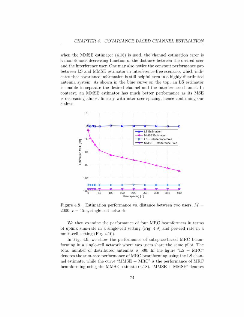
CHAPTER 4. COVARIANCE BASED CHANNEL ESTIMATION
when the MMSE estimator (4.18) is used, the channel estimation error isa monotonous decreasing function of the distance between the desired userand the interference user. One may also notice the constant performance gapbetween LS and MMSE estimator in interference-free scenario, which indi-cates that covariance information is still helpful even in a highly distributedantenna system. As shown in the blue curve on the top, an LS estimatoris unable to separate the desired channel and the interference channel. Incontrast, an MMSE estimator has much better performance as its MSEis decreasing almost linearly with inter-user spacing, hence confirming ourclaims.
0 50 100 150 200 250 300 350 400−25
−20
−15
−10
−5
0
5
User spacing [m]
Est
imat
ion
MS
E [d
B]
LS EstimationMMSE EstimationLS − Interference FreeMMSE − Interference Free
Figure 4.8 – Estimation performance vs. distance between two users, M =2000, r = 15m, single-cell network.
We then examine the performance of four MRC beamformers in termsof uplink sum-rate in a single-cell setting (Fig. 4.9) and per-cell rate in amulti-cell setting (Fig. 4.10).
In Fig. 4.9, we show the performance of subspace-based MRC beam-forming in a single-cell network where two users share the same pilot. Thetotal number of distributed antennas is 500. In the figure “LS + MRC”denotes the sum-rate performance of MRC beamforming using the LS chan-nel estimate, while the curve “MMSE + MRC” is the performance of MRCbeamforming using the MMSE estimate (4.18). “MMSE + MMSE” denotes
74

CHAPTER 4. COVARIANCE BASED CHANNEL ESTIMATION
0 50 100 150 200 250 300 350 4000
5
10
15
20
25
30
Distance between two users [m]
Sum
−ra
te [b
its/s
ec/H
z]
LS + MRCMMSE + MRCMMSE + MMSESubspace MRC
Figure 4.9 – Uplink sum-rate vs. distance between 2 users, M = 500, r =15m, cell-edge SNR 20dB, single-cell network.
the performance curve of MMSE beamforming using MMSE channel esti-mate when channel covariances (including the interference covariances) areassumed known during both channel estimation and signal detection. Thesimulation shows the simple subspace-based method has a very good per-formance. Due to pilot contamination, the MRC beamformer using MMSEchannel estimate is not as good as subspace-based method. The reason isthat R1 and R2 generally have overlapping signal subspaces here. We mayalso notice that the subspace-based MRC beamformer has some slight per-formance gains over the MMSE beamformer.
Fig. 4.10 depicts the uplink per-cell rate achieved by the above-mentionedMRC beamformers as a function of scattering radius r. In the simulation wehave 7 hexagonal cells with one center cell and 6 surrounding cells. Each cellhas one user. All the users share the same pilot sequence. The per-cell rateis defined as the sum-rate (6.19) divided by the number of cells. As can beseen, the subspace-based beamforming shows performance gains over othertraditional MRC methods especially when the radius of scattering ring issmaller. It also shows more robustness than MMSE beamformer when theradius of the scattering ring is larger.
75

CHAPTER 4. COVARIANCE BASED CHANNEL ESTIMATION
0 5 10 15 20 25 305
10
15
20
Radius of scattering ring [m]
Per
−ce
ll ra
te [b
its/s
ec/H
z]
LS + MRCMMSE + MRCMMSE + MMSESubspace MRC
Figure 4.10 – Uplink per-cell rate vs. r, cell-edge SNR 20dB, 7-cell network,each cell has M = 500 distributed antennas.
4.8 Discussions
In this chapter, we assumed the individual covariance matrices can beestimated separately. This could be done in practice by exploiting resourceblocks where the desired user and interference users are known to be as-signed at different times. In future networks, one may imagine a specifictraining design for learning second-order statistics. Since covariance infor-mation varies much slower than fast fading, such training may not consumea substantial amount of resources.
4.9 Conclusions
This chapter proposes a covariance-aided channel estimation frameworkin the context of interference-limited multi-cell multiple antenna systems.We develop Bayesian estimators and demonstrate analytically the efficiencyof such an approach for large-scale antenna systems, leading to a completeremoval of pilot contamination effects in the case covariance matrices sat-isfy a certain non-overlapping condition on their dominant subspaces. Wepropose a coordinated pilot assignment strategy that helps shape covariancematrices toward satisfying the needed condition and show channel estima-
76

CHAPTER 4. COVARIANCE BASED CHANNEL ESTIMATION
tion performance close to interference-free scenarios.We also put forward a modified MRC beamformer relaying on chan-
nel covariance’s low-rankness property. Simulation in a distributed antennasystem shows that such a low-complexity method approaches and even out-performs the MMSE beamformer which has higher complexity.
77

CHAPTER 4. COVARIANCE BASED CHANNEL ESTIMATION
78

Chapter 5
Joint Angle/Power basedDecontamination
5.1 Introduction
In chapter 4 we have shown several interference mitigation techniquesbased on the long-term statistics of user channels. Asymptotic performanceanalysis indicates that interference can in principle be discriminated on thebasis of the distributions of multipath AoAs. In particular, we demonstratedthat in the case when the AoA support of the desired user does not overlapwith the AoA supports of the interference users, an MMSE-based methodachieves full interference elimination. However, when such a non-overlappingcondition is not satisfied, interference persists in MMSE estimation, whichlimits the ultimate performance of massive MIMO. In this chapter, we seekto solve the remaining interference by exploiting the short-term statistics ofchannel information.
Two key features of massive MIMO channels that have been previouslyreported are of particular interest here: 1) channels of different users tend tobe pairwise orthogonal when the number of antennas increases, thus leadingto a specific subspace structure for the received data vectors that dependon these channels [28] and 2) the channel covariance matrix exhibits a low-rankness property whenever the multipath impinging on the MIMO arrayspans a finite angular spread [17,36,82]. The blind signal subspace estimationin [28] capitalizes on the first property. The second property has been utilizedin [6,17,36,82,83] assuming the complete knowledge of the long-term channelcovariance matrices. While the exploitation of the two properties individuallyhas given rise to a set of distinct original decontamination approaches, in
79
CHAPTER 5. JOINT ANGLE/POWER BASED DECONTAMINATION
this work we will exploit these two key features in a combined manner. Doingso we can propose a novel approach towards mitigating pilot contaminationthat exhibits much higher levels of robustness.
More specifically, in [28, 29], the pairwise channel orthogonality prop-erty allows to blindly estimate the user-of-interest channel subspace anddiscriminate between user-of-interest signals and interference based on thechannel powers. In practice, decontamination occurs via a projection drivenby the channel amplitudes. This approach works well within the constraintthat the interference channel is received with a power level sufficiently lowerthan that of the desired channel, a condition which is hard to guarantee forsome edge-of-cell terminals.
In a way completely different from [28,29], another approach based on aMMSE estimator is adopted in [36] to estimate the channel of interest viaprojection of the received signals onto the user-of-interest subspace. Thissubspace, identified by a channel covariance matrix (a long-term one, as op-posed to the instantaneous signal correlation matrix of [28,29]), is related tothe angular spread of the signal of interest [36] and enables to annihilate theinterference from users with non-overlapping domains of multipath angles-of-arrival (AoA). Interestingly, this latter approach makes no assumptionon received signal amplitudes and can also discriminate against interferingusers that are received with similar or even higher powers. Yet, the approachfails to decontaminate pilots when propagation scattering creates large anglespread, causing spatial overlapping among desired and interference channels.
In this chapter, we point out that the strengths of these two previ-ously unrelated estimation methods are strongly complementary, offeringa unique opportunity for developing robust massive MIMO channel estima-tion schemes. Thus, we aim to properly merge the two projections in comple-mentary domains while keeping the individual benefits. In fact, we proposea family of algorithms striking various performance/complexity trade-offs.
We start by presenting a first scheme named “covariance-aided ampli-tude based projection” that effectively combines projections in the angularand amplitude domains and exhibits robustness to interference power/anglesoverlapping conditions. We present an asymptotic analysis which reveals theconditions under which the channel estimation error due to pilot contami-nation and noise can be made to vanish. An intuitive physical interpretationof this condition for a ULA is given in the form of the residual interferencechannel energy contained in the multipath components that overlap in an-gle with those of the desired channel. Although the physical explanation isgiven for the ULA example, the general principle apply to other antennaplacement topologies.
80

CHAPTER 5. JOINT ANGLE/POWER BASED DECONTAMINATION
The obtained condition for decontamination is in general less restric-tive than the condition required by previous MMSE and the amplitudeprojection-based methods taken separately to achieve complete removal ofpilot contamination.
Following this, we then propose two low-complexity alternative schemescalled “subspace and amplitude based projection” and “MMSE + amplitudebased projection” respectively. Such schemes achieve different complexity-performance trade-off at moderate number of antennas. Specifically, the“subspace and amplitude based projection” can be shown to reach asymp-totic (in the number of antennas) decontamination result under the samechannel topology conditions as the first scheme.
5.2 UL Training/Data Transmission
Consider a multi-user multi-cell network with K users in each cell servedby their own BS. Recall from chapter 3 the multi-user MIMO channel be-tween all K users in cell l and BS j:
H(j)l ,
[h
(j)l1 h
(j)l2 · · · h
(j)lK
], (5.1)
and the pilot matrix consists of all pilot sequences used by these K users:
S ,[s1 s2 · · · sK
]T. (5.2)
During the training phase, the received signal at the base station j is
Y(j) =L∑l=1
H(j)l S + N(j), (5.3)
where N(j) ∈ CM×τ is the spatially and temporally white additive Gaussiannoise (AWGN) with zero-mean and element-wise variance σ2
n. Then, duringthe uplink data transmission phase, each user transmits C data symbols.The received data signal at base station j is given by:
W(j) =
L∑l=1
H(j)l Xl + Z(j), (5.4)
where Xl ∈ CK×C is the matrix of transmitted symbols of all users in the l-th cell. The symbols are i.i.d. with zero-mean and unit average element-wisevariance. Z(j) ∈ CM×C is the AWGN noise with zero-mean and element-wise variance σ2
n. Note that the block fading channel is constant during thetransmission for the τ pilot symbols and the C data symbols.
81

CHAPTER 5. JOINT ANGLE/POWER BASED DECONTAMINATION
5.3 A review of LMMSE estimation
We briefly recall the MMSE channel estimator in a multi-cell single-userper cell setting. Without loss of generality, we assume cell j is the target
cell, and h(j)j ∈ CM×1 is the desired channel, while h
(j)l ∈ CM×1, ∀l 6= j are
the interference channels. We rewrite (5.3) in a vectorized form,
y(j) = S
L∑l=1
h(j)l + n(j), (5.5)
where y(j) = vec(Y(j)), n(j) = vec(N(j)). A pilot sequence s is shared by allusers. The pilot matrix S is given by
S , s⊗ IM . (5.6)
We define the channel covariance matrices
R(j)l , E{h(j)
l h(j)Hl } ∈ CM×M , l = 1, . . . , L. (5.7)
A linear MMSE estimator for h(j)j is given by
h(j)MMSEj = R
(j)j
(τ(
L∑l=1
R(j)l ) + σ2
nIM
)−1
SH
y(j). (5.8)
5.3.1 Asymptotic performance of MMSE
As shown in chapter 4, for a base station equipped with a ULA, the aboveMMSE estimator can fully eliminate the effects of interfering channels whenM → ∞, under a specific “non overlap” condition on the distributions ofmultipath AoAs for the desired and interference channels. This conditionis formalized as follows: Assume the user in cell j is our target (desireduser). Denote the angular support of the desired channel as Φd, (i.e., the
probability density function (PDF) pd(θ) of the AoA of desired channel h(j)j
satisfies pd(θ) > 0 if θ ∈ Φd and pd(θ) = 0 if θ /∈ Φd) and similarly the
union of the angular supports of all interference channels h(j)l (l 6= j) as
Φi. If Φd ∩ Φi = ∅, then, as M → ∞, (5.8) converges to an interference-free estimate. In practice the “non overlap” condition is hard to guaranteeand the finite-M performance of the MMSE scheme will depend on angularspreading and user location, although the latter can be shaped via the useof so-called coordinated pilot assignment [36].
82

CHAPTER 5. JOINT ANGLE/POWER BASED DECONTAMINATION
5.4 A review of power domain discrimination
Interestingly, angle is not the only domain where interference can bediscriminated upon, as revealed from a completely different approach topilot decontamination [28,29]. In that approach the empirical instantaneouscovariance matrix built from the received data (5.4) is exploited, in contrastwith the use of long-term covariance matrices in (5.8). Assume cell j is ourtarget cell and each cell has K users. The eigenvalue decomposition (EVD)of W(j)W(j)H/C is written as
1
CW(j)W(j)H = U(j)Λ(j)U(j)H , (5.9)
where U(j) ∈ CM×M = [u(j)1 |u
(j)2 | · · · |u
(j)M ] is a unitary matrix and Λ(j) =
diag{λ(j)1 , · · · , λ(j)
M } with its diagonal entries sorted in a non-increasing order.By extracting the first K columns of U(j), i.e., the eigenvectors correspond-ing to the strongest K eigenvalues, we obtain an orthogonal basis
E(j) ,[u
(j)1 u
(j)2 · · · u
(j)K
]∈ CM×K . (5.10)
The basic idea in [28, 29] is to use the orthogonal basis E(j) as an estimate
for the span of H(j)j , which includes all desired user channels in cell j. Then,
by projecting the received signal onto the subspace spanned by E(j), mostof the signal of interest is preserved. In contrast, the interference signal iscanceled out thanks to the asymptotic property that the user channels arepairwise orthogonal as the number of antennas tends to infinity. Thus after
the above mentioned projection, the estimate of the multi-user channel H(j)j
is given by:
H(j)AMj =
1
τE(j)E(j)HY(j)SH . (5.11)
Note here that interference and desired channel directions are discriminatedon the basis of channel amplitudes and not AoA, hence the estimate islabeled “AM” for “Amplitude”. As a way to guarantee an asymptotic sepa-ration between the signal of interest and the interference in terms of power,it has been suggested to introduce power control in the network [28,29].
5.4.1 Generalized amplitude projection
As shown in [28, 29], the above method works well when the desiredchannels and interference channels are separable in power domain, i.e., the
83

CHAPTER 5. JOINT ANGLE/POWER BASED DECONTAMINATION
instantaneous powers of any desired channels are higher than that of anyinterference channels. In practice however, this assumption is not alwaysguaranteed. For a finite number of antennas, the short-term fading realiza-tion can cause the interference subspace to spill over the desired one. Anenhanced version can somewhat mitigate this problem by considering a gen-eralized amplitude based projection. This consists in selecting a possiblylarger number (κ(j)) of dominant eigenvectors to form E(j), where κ(j) is
the number of eigenvalues in Λ(j) that are greater than µλ(j)K . µ is a design
parameter that satisfies 0 ≤ µ < 1. See section 5.7 for details on the choiceof µ.
5.5 Covariance-aided amplitude based projection
Note that both previous methods, while being able to tackle pilot con-tamination in quite different ways, perform well only in some restricteduser/channel topologies. For a ULA base station, the MMSE method leadsto interference free channel estimates under the strict requirement that thedesired and interference channel do not overlap in their AoA regions. Whilethe amplitude based projection requires that no interference channel powerexceeds that of a desired channel to achieve a similar result. Unfortunately,due to the random user location and scattering effects, it is quite unlikelyto achieve these conditions at all times. As a result, by combining the usefulproperties of both the MMSE and the amplitude projection method, we pro-pose below novel estimation methods that will lead to enhanced robustnessin a realistic cellular scenario.
5.5.1 Single user per cell
For ease of exposition we first consider a simplified scenario where intra-cell interference is ignored by assuming that each cell has only one user, i.e.,K = 1. The users in different cells share the same pilot sequence s. Thenwith proper modifications we will generalize this method to the setting ofmultiple users per cell in section 5.5.3.
The objective is to combine long-term statistics which include spatial dis-tribution information together with short-term empirical covariance whichcontains instantaneous amplitude and direction channel information. Hence,a spatial distribution filter can be associated to an instantaneous projectionoperator to help discriminate against any interference terms whose spatialdirections live in a subspace orthogonal to that of the desired channel. The
84
CHAPTER 5. JOINT ANGLE/POWER BASED DECONTAMINATION
intuition is that such a spatial filter may bring the residual interferenceto a level that is acceptable to the instantaneous projection-based channelestimator.
In order to carry out the above intuition, we introduce a long-term sta-tistical filter Ξj , which is based on channel covariance matrices in a waysimilar to that used by the MMSE filter in (5.8).
Ξj =
(L∑l=1
R(j)l + σ2
nIM
)−1
R(j)j . (5.12)
Note that the linear filter Ξj allows to discriminate against the inter-ference in angular domain by projecting away from multipath AoAs thatare occupied by interference. Note also that the choice of spatial filter Ξj
is justified from the fact that the full information of desired channel h(j)j is
preserved, as h(j)j lies in the signal space of R
(j)j . In fact, the desired channel
is recoverable using another linear transformation Ξj′:
Ξj′ , R
(j)†
j
(L∑l=1
R(j)l + σ2
nIM
), (5.13)
as can be seen from the following equality
Ξ′jΞjh(j)j = R
(j)†j R
(j)j h
(j)j = VjV
Hj h
(j)j = h
(j)j , (5.14)
where the columns of Vj are the eigenvectors of R(j)j corresponding to non-
zero eigenvalues.
The spatial filter is applied to the received data signal at base station jas
Wj , ΞjW(j). (5.15)
The amplitude-based method as shown in section 5.4 can now be appliedon the filtered received data to get rid of the residual interference. Take theeigenvector corresponding to the largest eigenvalue of the matrix WjW
Hj /C:
uj1 = e1{1
CWjW
Hj }. (5.16)
Hence uj1 can be considered as an estimate of the direction of the vector
Ξjh(j)j .
85

CHAPTER 5. JOINT ANGLE/POWER BASED DECONTAMINATION
We then cancel the effect of the pre-multiplicative matrix Ξj using Ξ′jin (5.13), and we obtain an estimate of the direction of the channel vector
h(j)j as follows:
uj1 =Ξ′juj1∥∥∥Ξ′juj1∥∥∥
2
. (5.17)
Finally, the phase and amplitude ambiguities of the desire channel canbe resolved by projecting the LS estimate onto the subspace spanned by uj1:
h(j)CAj =
1
τuj1u
Hj1Y
(j)s∗, (5.18)
where the superscript “CA” denotes the covariance-aided amplitude domainprojection.
The algorithm is summarized below:
Algorithm 2 Covariance-aided Amplitude based Projection
1: Take the first eigenvector of WjWHj /C as in (5.16), with Wj being the
filtered data signal.2: Reverse the effect of the spatial filter using (5.17).3: Resolve the phase and amplitude ambiguities by (5.18).
The complexity of this proposed estimation scheme is briefly evaluated.
We note that the computation of the matrix inversions in (5.12) has acomplexity order of O(M2.37). However, these computations are performedin a preamble phase and their cost is negligible under the underlying as-sumption of channel stationarity implicitly made in this article. In practicalsystems, the matrix inversion in (5.12) is performed when the channel statis-tics are updated. Since the channel statistics are typically updated in a timescale much larger than the channel coherence time, i.e., the time scale forthe applicability of Algorithm 2, then their computational cost is negligible.Therefore, we can focus on the complexity of Algorithm 2 only.
In step 1, the spatial filtering of the data signals in (5.15) and the com-
putation of the covariance matrix WjWHj is performed along with the com-
putation of the dominant eigenvector of an M × M matrix as in (5.16).The former computation has a complexity order O(CM2) while, by apply-ing the classical power method, the computation of the dominant vector hasa complexity order O(M2). Both step 2 and step 3 require multiplications ofmatrices by M -dimensional vectors and thus both have a complexity order
86

CHAPTER 5. JOINT ANGLE/POWER BASED DECONTAMINATION
O(M2). Then, the global complexity of the algorithm is dominated by thecomplexity of step 1, which is O(CM2).
The ability for the above estimator to combine the advantages of thepreviously known angle and amplitude projection based estimators is nowanalyzed theoretically. In particular we are interested in the conditions underwhich full pilot decontamination can be achieved asymptotically in the limitof the number of antennas M and data symbols C. In order to facilitate theanalysis, we introduce the following condition:
Condition C1 : The spectral norm of R(j)l is uniformly bounded:
∀M ∈ Z+ and ∀l ∈ {1, . . . , L}, ∃ζ, s.t.∥∥∥R(j)
l
∥∥∥2< ζ, (5.19)
where Z+ is the set of positive integers, and ζ is a constant.Condition C1 can be interpreted as describing all the scenarios in which
the channel energy is spread over a subspace whose dimension grows with M .Note that the same assumption can be found in some other papers, e.g., [70].The corresponding physical condition for a ULA has been analyzed in section3.5.
As another interpretation of the condition, it is worth noting that whenthis condition is not satisfied, there is no guarantee that the asymptoticpairwise orthogonality of different users’ channels holds. In other words, the
quantity h(j)Hj h
(j)l /M, l 6= j may not converge to zero, which is an adverse
condition for all massive MIMO methods. However our proposed methodsstill have significant performance gains under this adverse circumstance.Moreover, C1 is a sufficient condition and we believe it can be weakened.
5.5.2 Asymptotic performance of the proposed CA estimator
We now look into the performance analysis of the proposed estimationscheme. Let us define
α(j)l , lim
M→∞
1
Mtr{ΞjR
(j)l ΞH
j },∀l = 1, . . . , L. (5.20)
Theorem 4. Given condition C1, if the following inequality holds true:
α(j)j > α
(j)l ,∀l 6= j, (5.21)
then, the estimation error of (5.18) vanishes:
limM,C→∞
∥∥∥h(j)CAj − h
(j)j
∥∥∥2
2∥∥∥h(j)j
∥∥∥2
2
= 0. (5.22)
87

CHAPTER 5. JOINT ANGLE/POWER BASED DECONTAMINATION
Proof: For the sake of notational convenience, in this proof we assumethe user in cell j is the target user and thus drop the superscript (j). The
desired channel is denoted by hj = h(j)j and the interference channels are
hl = h(j)l , l 6= j. Since hl, l = 1, . . . , L, is considered as M × 1 complex
Gaussian with the spatial correlation matrices Rl = E{hlhHl }, the channelscan be factorized as [75]
hl = R1/2l hWl, l = 1, . . . , L, (5.23)
where hWl ∼ CN (0, IM ), is i.i.d. M × 1 vector with unit variance. Webuild the proof of Theorem 4 on the general correlation model (6.6). Theproof consists in three parts, corresponding to the three steps in Algorithm2 respectively. More specifically, Lemma 3 (and the intermediate resultstowards Lemma 3) is the first part of the proof. It shows that uj1 alignsasymptotically with the direction of the filtered channel vector hj = Ξjhj .The second part of the proof is provided in Lemma 8, which proves that aftercanceling the effect of the spatial filter using Ξ′j , we obtain the directionof the true channel hj in uj1. The final part of the proof shows that byprojecting the LS estimate onto the subspace of uj1, we resolve the phaseand amplitude of the true channel.
Lemma 3. Given condition C1, if α(j)j > α
(j)l , ∀l 6= j, then there exists a
unique 0 ≤ φ < 2π, such that
limM,C→∞
∥∥∥∥∥ hj∥∥hj∥∥2
− uj1ejφ
∥∥∥∥∥2
= 0. (5.24)
where hl , Ξjhl, l = 1, . . . , L.
Proof: The proof of Lemma 3 relies on several intermediate results, namelyLemma 4 - Lemma 7.
Lemma 4. Under condition C1, the spectral norm of ΞjΞHj satisfies:
limM→∞
1
M
∥∥ΞjΞHj
∥∥2
= 0. (5.25)
Proof: See Appendix .8.Lemma 4 indicates that the spectral norm of the covariance of the noise (aftermultiplying Ξj) is bounded and does not scale with M . This conclusion willbe exploited when we prove in Lemma 7 that the impact of noise on thedominant eigenvector/eigenvalue vanishes.
88

CHAPTER 5. JOINT ANGLE/POWER BASED DECONTAMINATION
Lemma 5. [84] Let AM be a deterministic M ×M complex matrix withuniformly bounded spectral radius for all M . Let q = 1√
(M)[q1, · · · , qM ]T
where qi,∀i = 1, · · · ,M is i.i.d. complex random variable with zero mean,unit variance, and finite eighth moment. Let r be a similar vector indepen-dent of q. Then as M →∞,
qHAMqa.s.−−→ 1
Mtr{AM}, (5.26)
and
qHAMra.s.−−→0, (5.27)
wherea.s.−−→ denotes almost sure convergence.
Note that in this chapter, the condition on the finite eighth momentalways holds, as when we apply Lemma 5, the components of the vector ofinterest are i.i.d. complex Gaussian variables. It is well known that a complexGaussian variable with zero mean, unit variance has finite eighth moment.
Lemma 6. Given condition C1,
limM→∞
1
MhHj hl = 0,∀l 6= j (5.28)
limM→∞
1
MhHl hl
a.s.= αl, l = 1, . . . , L. (5.29)
Proof: See Appendix .9.
Lemma 7. When condition C1 is satisfied,
limM,C→∞
∥∥∥∥∥WjWHj
MC
hj∥∥hj∥∥2
− αjhj∥∥hj∥∥2
∥∥∥∥∥2
= 0, (5.30)
Proof: See Appendix .10.
Lemma 7 proves that as M,C → ∞, αj is an asymptotic eigenvalue of the
random matrix WjWHj /MC, with its corresponding eigenvector converging
to hj/∥∥hj∥∥2
up to a random phase.
We now return to the proof of Lemma 3. Since αj > αl,∀l 6= j, one mayreadily obtain from Lemma 7 and (5.28):
limM,C→∞
λ1
{WjW
Hj
MC
}= αj , (5.31)
89

CHAPTER 5. JOINT ANGLE/POWER BASED DECONTAMINATION
and that there exists a unique 0 ≤ φ < 2π, such that
limM,C→∞
∥∥∥∥∥ hj∥∥hj∥∥2
− e1
{WjW
Hj
MC
}ejφ
∥∥∥∥∥2
= 0, (5.32)
which completes the proof of Lemma 3.
Now we show the second part of the proof of Theorem 4. Note that inthis part we make the implicit assumption that the spectral norm of Ξ′j
satisfies∥∥∥Ξ′j∥∥∥
2< +∞. A sufficient (but not necessary) condition of such an
assumption is that the spectral norm of R†j is finite.
Lemma 8. Given (5.24), we have
limM,C→∞
∥∥∥∥ hj‖hj‖2
− uj1ejφ
∥∥∥∥2
= 0. (5.33)
Proof: See Appendix .11.
The final part of the proof of Theorem 4 can be found in Appendix .12,which corresponds to step 3 of Algorithm 2. The proof shows that projectingthe LS estimate onto the subspace of uj1 will lead to noise-free estimateasymptotically as M,C →∞. This concludes the proof of Theorem 4.
Interestingly, condition (5.21) in Theorem 4 can be replaced with∥∥∥Ξjh(j)j
∥∥∥2>∥∥∥Ξjh
(j)l
∥∥∥2, ∀l 6= j, (5.34)
which indicates that under suitable conditions on the spectral norm of chan-nel covariance, after multiplying the filter Ξj , if the power of the desiredchannel is higher than that of interference channel, then, pilot contamina-tion disappears asymptotically, along with noise.
Note that we have so far no assumption on antenna placement in theanalysis, other than the requirement for uniformly boundedness of the spec-tral norm of channel covariance. In the sequel we look into a specific modelof ULA as an example and seek to further understand the physical meaningof the proposed method.
We still assume h(j)j is the channel of interest. Denote its angular support
as Φd. Decompose the interference channel h(j)l ,∀l 6= j, as follows:
h(j)l = h
(j)li + h
(j)lo , (5.35)
90

CHAPTER 5. JOINT ANGLE/POWER BASED DECONTAMINATION
where
h(j)li =
β(j)l√P
∑θ∈Φd
a(θ)eiϕθ (5.36)
h(j)lo =
β(j)l√P
∑θ/∈Φd
a(θ)eiϕθ , (5.37)
which means h(j)li is the residual multipath component of the interference
channel within the AoA region Φd of the desired channel, while h(j)lo is the
multipath component which is outside Φd.
Theorem 5. For a ULA base station, under condition C1, if the residualmultipath component of the interference channel satisfies:
∀l 6= j,∥∥∥Ξjh
(j)li
∥∥∥2<∥∥∥Ξjh
(j)j
∥∥∥2, (5.38)
then, the estimation error of the estimator (5.18) vanishes:
limM,C→∞
∥∥∥h(j)CAj − h
(j)j
∥∥∥2
2∥∥∥h(j)j
∥∥∥2
2
= 0. (5.39)
Proof: See Appendix .13.Theorem 5 further confirms the fact that for a base station equipped withULA, only the interference multipath components that overlap with thoseof the desired channel affect the performance of our pilot decontaminationmethod. In other words, the spatial filter Ξj removes the energy located inall interference multipath originating from directions that do not overlapwith those of the desired channel. It is then sufficient for the energy of theresidual interference components to be below that of the desired channel toallow for a full decontamination.
5.5.3 Generalization to multiple users per cell
Now we generalize the covariance-aided amplitude based projection intomulti-user setting where K users are served simultaneously in each cell. We
consider the estimation of user channel h(j)jk in the reminder of this section.
Define a matrix H(j)j\k as a sub-matrix of H
(j)j after removing its k-th
column:H
(j)j\k ,
[h
(j)j1 · · · h
(j)j(k−1) h
(j)j(k+1) · · · h
(j)jK
]. (5.40)
91

CHAPTER 5. JOINT ANGLE/POWER BASED DECONTAMINATION
A corresponding estimate of (5.40), denoted by H(j)j\k, is obtained by remov-
ing the k-th column of H(j)j , which can be an LS estimate, MMSE estimate,
or other linear/non-linear estimate of H(j)j . For demonstration purpose only,
in this thesis we use the simplest LS estimate, which already shows verygood performance.
In order to adapt the method in section 5.5.1 to multi-user scenario,we propose to first neutralize the intra-cell interference with a Zero-Forcing
(ZF) filter Tjk based on the LS estimate H(j)j\k, and then apply the spatial
filter Ξjk. After these two filters, the data signal is now:
Wjk , ΞjkTjkW(j), (5.41)
whereTjk , IM − H
(j)j\k(H
(j)Hj\k H
(j)j\k)
−1H(j)Hj\k , (5.42)
and
Ξjk ,
(L∑l=1
R(j)lk + σ2
nIM
)−1
R(j)jk . (5.43)
The rest of this method proceeds as in the single user setting. Take thedominant eigenvector of WjkW
Hjk/C:
ujk1 = e1{1
CWjkW
Hjk}. (5.44)
The estimate of the direction of h(j)jk is obtained by:
ujk1 =Ξ′jkujk1∥∥∥Ξ′jkujk1
∥∥∥2
, (5.45)
where
Ξ′jk , R(j)†jk
(L∑l=1
R(j)lk + σ2
nIM
). (5.46)
Finally the phase and amplitude ambiguities are resolved by the training
sequence, and we have the estimate of h(j)jk :
h(j)CAjk =
1
τujk1u
Hjk1Y
(j)SH . (5.47)
Note that in this method, we build the ZF type filter Tjk based on a rough LSestimate. Further improvements can be attained with higher quality estimate
92

CHAPTER 5. JOINT ANGLE/POWER BASED DECONTAMINATION
at the cost of higher complexity. As a simple example, we can reduce the
effect of noise on the estimate H(j)j\k by first applying EVD of W(j)W(j)H/C,
then removing the subspace where the noise lies, and finally performing LSestimation. These extensions are out of the scope of this thesis.
5.6 Low-complexity alternatives
In this section, we propose two alternatives of the method shown insection 5.5, aiming at lower computational complexity at the cost of mildperformance loss.
5.6.1 Subspace and amplitude based projection
The low-rankness of channel covariance implies that the uplink receiveddesired signal lives in a reduced subspace. By projecting the received data
signal W(j) onto the signal space of R(j)jk , we are able to preserve the signal
from user k in cell j while remove the interference and noise that live in itscomplementary subspace. In the following, we show a subspace-based signalspace projection method that relies on the covariance of desired channelonly. For ease of exposition, we simplify the system setup to single user percell. Let the user in cell j be the target user. The EVD of the covariance ofthe desired channel is
R(j)j = Vj ΣjV
Hj , (5.48)
where the diagonal entries of Σj contains the non-negligible eigenvalues of
R(j)j . Then we project the received data signal onto the signal space of R
(j)j ,
or the column space of Vj :
Wj , VjVHj W(j). (5.49)
The rest of this method follows the same idea as the covariance-aided ampli-tude based projection scheme. Taking the eigenvector corresponding to the
largest eigenvalue of WjWHj /C:
uj1 = e1
{1
CWjW
Hj
}, (5.50)
the channel estimate of h(j)j is given by
h(j)SAj =
1
τuj1u
Hj1Y
(j)s∗, (5.51)
93

CHAPTER 5. JOINT ANGLE/POWER BASED DECONTAMINATION
where the superscript“SA”stands for“subspace and amplitude based projec-tion”. Note that this method does not require the covariance of interferencechannels or variance of noise. It explicitly relies on the assumption that thedesired covariance matrix has a low-dimensional signal subspace, with somedegradations expected when this condition is not realized in practice. In
fact, if R(j)j has full rank, this method degrades to pure amplitude based
projection.Note that this “SA” estimator has lower complexity than the “CA” esti-
mator (5.18) in the sense that 1) “SA” estimator does not require the sta-tistical knowledge of the interference channels or the variance of the noise,and 2) “SA” estimator skips step 2 in Algorithm 2.
The physical condition under which full decontamination is achieved withthis method is shown below in the case of a ULA. We denote the angular
support of desired channel h(j)j by Φd and the multipath components of the
interference channel h(j)l falling in Φd as h
(j)li .
Theorem 6. For a ULA base station, if the power of interference channelthat falls into the angular support Φd satisfies
∀l 6= j,∥∥∥h(j)
li
∥∥∥2<∥∥∥h(j)
j
∥∥∥2, (5.52)
and the channel covariance satisfies
∀M ∈ Z+, ∀l 6= j,
∥∥∥∥R(j) 12
j VjVHj R
(j) 12
l
∥∥∥∥2
< +∞, (5.53)
then, the estimation error of the estimator (5.51) vanishes:
limM,C→∞
∥∥∥h(j)SAj − h
(j)j
∥∥∥2
2∥∥∥h(j)j
∥∥∥2
2
= 0. (5.54)
Proof: Due to lack of space, we skip the complete proof and only givetwo key steps below. By applying the asymptotic orthogonality between twosteering vectors which are associated with different AoAs ( Lemma 3 in [36]),we may readily obtain:
limM→∞
1√M
VjVHj h
(j)j =
1√M
h(j)j (5.55)
limM→∞
1√M
VjVHj h
(j)l =
1√M
h(j)li , ∀l 6= j, (5.56)
94

CHAPTER 5. JOINT ANGLE/POWER BASED DECONTAMINATION
which means the multipath components of interference that fall outside Φd
disappear asymptotically after the projection by VjVHj . Then, equation
(5.53) ensures that
limM→∞
1
Mh
(j)Hj h
(j)l = 0, l 6= j, (5.57)
where
h(j)l , VjV
Hj h
(j)l , l = 1, . . . , L. (5.58)
Note that in Theorem 6 condition (5.53) is less restrictive than the uniformlyboundedness of the spectral norm of the channel covariance. In the specialcase of zero angular spread, the rank of channel covariance becomes one.Denote the deterministic AoA from the user in cell l to base station j as
θ(j)l . We can easily see that the channel estimation error of (5.51) vanishes
completely as M,C →∞ as long as
∀l 6= j, θ(j)l 6= θ
(j)j , (5.59)
which occurs with probability one.When channel covariance is not available, we can still benefit from the
subspace projection method by approximating Vj with a subset of discreteFourier transform (DFT) basis as shown in [85]. This DFT basis can bechosen based on a small number of channel observations. The generalizationto multi-user case can be done by introducing the ZF filter (5.42) as insection 5.5.3. Due to lack of space, we skip the details.
5.6.2 MMSE + amplitude based projection
Another alternative is to directly project the MMSE estimate onto thesubspace of E(j) obtained by EVD of W(j)W(j)H/C as in section 5.4. The
estimator for the multi-user channel H(j)j is given by:
H(j)MAj = E
(j)E
(j)HR
(j)j
(τ(
L∑l=1
R(j)l ) + σ2
nIKM
)−1
SH
y(j), (5.60)
where
E(j)
, IK ⊗E(j), (5.61)
95

CHAPTER 5. JOINT ANGLE/POWER BASED DECONTAMINATION
S , ST ⊗ IM =[
s1 ⊗ IM · · · sK ⊗ IM], (5.62)
andR
(j)l = diag{R(j)
l1 , ...,R(j)lK}, l = 1, . . . , L. (5.63)
The superscript “MA” denotes MMSE + amplitude based projection. It isworth noting that both the amplitude-based projection and angular-basedprojection require large number of antennas to achieve complete decontami-nation. In contrast, the MMSE estimator is efficient with very small numberof antennas. As M grows, MMSE estimator starts to reduce interferenceearlier than the previously proposed methods, as will be shown by simula-tions in section 5.7. However, unlike the previously proposed schemes, this“MA”estimator cannot achieve complete decontamination when the interfer-ence channel is overlapping with desired channel in both angular and powerdomains.
5.7 Numerical Results
This section contains numerical results of our different channel estima-tion schemes compared with prior methods. In the simulation, we have mul-tiple hexagonally shaped adjacent cells in the network. The radius of eachcell is 1000 meters. Each base station has M antennas, which forms a ULA,with half wavelength antenna spacing. The length of pilot sequence is τ = 10.
Two performance metrics are considered. The first is the normalizedchannel estimation error
ε ,1
KL
L∑j=1
K∑k=1
∥∥∥h(j)
jk − h(j)jk
∥∥∥2
2∥∥∥h(j)jk
∥∥∥2
2
. (5.64)
The estimation errors in the plots are obtained in Monte Carlo simulationsand finally displayed in dB scale.
The second metric is the uplink per-cell rate when MRC receiver (basedon the obtained channel estimate) is used at base station side.
In all simulations presented in this section, we assume that the channelcovariance matrix is estimated using 1000 exact channel realizations. Themultipath angle of arrival of any channel (including the interference channel)follows a uniform distribution centered at the direction corresponding toline-of-sight (LoS). The number of multipath is P = 50. According to thecoherence time model in [86], for a mobile user moving at a vehicular speedof 70 km/h in an environment of 2.6 GHz carrier frequency and 5µs high
96

CHAPTER 5. JOINT ANGLE/POWER BASED DECONTAMINATION
0 50 100 150 200 250 300 350 400 450 500−20
−15
−10
−5
0
5
Number of Antennas
Est
imat
ion
Err
or [d
B]
LS estimationPure MMSEPure amplitudeMMSE + amplitudeCovariance−aided amplitudeMMSE − no interference
Figure 5.1 – Estimation performance vs. M, 2-cell network, 1 user per cell,path loss exponent γ = 0, partially overlapping angular support, AoA spread60 degrees, SNR = 0 dB.
delay spread (corresponding to an excess distance of 1.5 km), the channelcan be assumed coherent over 500 transmitted symbols. Thus we will letC = 500 in simulations, although larger coherence time can be expected inpractice for a user with lower mobility.
Note that in all simulations, the amplitude-based projection and MMSE+ amplitude based projection follow the enhanced eigenvector selectionstrategy shown in section 5.4.1 with the design parameter µ = 0.2.
We first illustrate Theorem 4 in Fig. 5.1. Suppose we have a two-cellnetwork, with each cell having one user. In order to make the interferenceoverlapping in power domain with the desired signal, we set the path lossexponent γ = 0. The power of the interference channel has equal probabilityto be higher or lower than the power of the desired channel. The user ineach cell is deliberately put in a symmetrical position such that the multi-path angular supports of the interference and the desired channel are halfoverlapping with each other.
In the figure, “LS estimation” and “Pure MMSE” denote the system per-formances when an LS estimator and an MMSE estimator (5.8) are used re-spectively. “Pure amplitude” denotes the case when we apply the generalizedamplitude based projection method only. “MMSE + amplitude” represents
97

CHAPTER 5. JOINT ANGLE/POWER BASED DECONTAMINATION
0 50 100 150 200 250 300 350 400 450 500−25
−20
−15
−10
−5
0
5
Number of Antennas
Est
imat
ion
Err
or [d
B]
LS estimationPure MMSEPure amplitudeMMSE + amplitudeCovariance−aided amplitude
Figure 5.2 – Estimation performance vs. M, 7-cell network, one user per cell,AoA spread 30 degrees, path loss exponent γ = 2, cell-edge SNR = 0 dB.
the proposed estimator (5.60). “Covariance-aided amplitude” denotes theproposed covariance-aided amplitude based projection method (5.18). Thecurve “MMSE - no interference” shows the estimation error of an MMSEestimator in an interference-free scenario. As can be seen from Fig. 5.1, dueto the overlapping interference in both angle and power domains, the per-formance of all estimators saturate quickly with the number of antennas,except the proposed covariance-aided amplitude based projection method,which eventually outperforms interference-free MMSE estimation. 1
In Fig. 5.2 and Fig. 5.3, we show the performance of estimation errorand the corresponding uplink per-cell rate for a 7-cell network, with singleuser per cell. The users are assumed to be distributed randomly and uni-formly within their own cells excluding a central disc with radius 100 meters.The angular spread of the user channel (including interference channel) is30 degrees. The path loss exponent is now γ = 2. As we may observe, thetraditional LS estimator suffers from severe pilot contamination. The pureamplitude based method and the pure MMSE method alleviate the pilot
1. The reason is that the performance of the interference-free MMSE estimation has anon-vanishing lower bound due to white Gaussian noise. On the contrary, our proposedcovariance-aided amplitude based projection method eliminates the effects of noise andinterference asymptotically.
98

CHAPTER 5. JOINT ANGLE/POWER BASED DECONTAMINATION
0 100 200 300 400 5002
3
4
5
6
7
8
9
10
11
Number of Antennas
Per
−ce
ll R
ate
[bps
]
LS estimationPure MMSEPure amplitudeMMSE + amplitudeCovariance−aided amplitude
Figure 5.3 – Uplink per-cell rate vs. M, 7-cell network, one user per cell,AoA spread 30 degrees, path loss exponent γ = 2, cell-edge SNR = 0 dB.
interference, yet saturate with the number of antennas. These saturationeffects come from the overlapping of the interference and the desired chan-nels in power and angular domains respectively. The “MMSE + amplitude”approach outperforms these two known methods as it discriminates againstinterference in both amplitude and angular domains. However this schemecannot cope with the case of overlapping in both domains. Owing to itsrobustness, the covariance-aided amplitude projection method outperformsthe rest in terms of both estimation error and uplink per-cell rate.
We now turn our attention to multi-cell multi-user scenario. Fig. 5.4 andFig. 5.5 show the channel estimation performance and the corresponding up-link per-cell rate for a 7-cell network with each cell having 4 users. In thesetwo figures, we add the curve of subspace and amplitude based projection,which is denoted in the figures as“Subspace + amplitude”. The other param-eters remain unchanged compared with those in Fig. 5.2 and Fig. 5.3. We cannotice that in Fig. 5.4 the covariance-aided amplitude projection method hassome performance loss with respect to the low-complexity MMSE + ampli-tude method and the MMSE method when the number of antennas is small.It is due to the following two facts: 1) when M is small, it is well knownthat MMSE works well, but not the amplitude based methods, and 2) withsmall M , the asymptotical orthogonality of channels of different users isnot fully exhibited, and consequently a small amount of signal of interest
99

CHAPTER 5. JOINT ANGLE/POWER BASED DECONTAMINATION
0 50 100 150 200 250 300 350 400 450 500−16
−14
−12
−10
−8
−6
−4
−2
0
2
4
Number of Antennas
Est
imat
ion
Err
or [d
B]
LS estimationPure MMSEPure amplitudeMMSE + amplitudeSubspace + amplitudeCovariance−aided amplitude
Figure 5.4 – Estimation performance vs. M, 7-cell network, 4 users per cell,AoA spread 30 degrees, path loss exponent γ = 2, cell-edge SNR = 0 dB.
0 100 200 300 400 5000
5
10
15
20
25
30
Number of Antennas
Per
−ce
ll R
ate
[bps
]
LS estimationPure MMSEPure amplitudeMMSE + amplitudeSubspace + amplitudeCovariance−aided amplitude
Figure 5.5 – Uplink per-cell rate vs. M, 7-cell network, 4 users per cell, AoAspread 30 degrees, path loss exponent γ = 2, cell-edge SNR = 0 dB.
100

CHAPTER 5. JOINT ANGLE/POWER BASED DECONTAMINATION
is removed by the ZF filter Tkj , along with intra-cell interference. Howeverit is not disturbing in the sense that 1) as the number of antennas grows,the covariance-aided amplitude projection method quickly outperforms theother methods; and 2) The per-cell rate of this proposed method is still goodeven with moderate number of antennas, e.g., M > 25. It is also interestingto note that the low-complexity alternative scheme, subspace and ampli-tude based projection method, has some minor performance loss, yet keepsapproximately the same slope as the covariance-aided amplitude projection.
5.8 Conclusions
In this chapter we proposed a series of robust channel estimation algo-rithms exploiting path diversity in both angle and amplitude domains. Thefirst method called “covariance-aided amplitude based projection” is robusteven when the desired channel and the interference channels overlap in multi-path AoA and are not separable just in terms of power. Two low-complexityalternative schemes were proposed, namely “subspace and amplitude basedprojection” and “MMSE + amplitude based projection”. Asymptotic analy-sis shows the condition under which the channel estimation error convergesto zero.
101

CHAPTER 5. JOINT ANGLE/POWER BASED DECONTAMINATION
102

Chapter 6
Cooperative FeedbackDesign in FDD
In previous chapters, we have addressed one of the fundamental problemsof massive MIMO - pilot contamination in TDD deployment. In this chapter,we deal with another challenge - CSI acquisition for massive MIMO in FDDsetting. In particular, we propose CSI feedback reduction methods basedon novel approaches of feedback design in FDD massive MIMO systems.We exploit the synergies between massive MIMO systems and inter-usercommunications based on D2D. The exchange of local CSI among users, en-abled by D2D communications, makes available global CSI at the terminals.Thus, we can construct more informative forms of feedback based on thisshared knowledge. Two feedback variants are highlighted: 1) cooperative CSIfeedback, and 2) cooperative precoder index feedback. For a given feedbackoverhead, the sum-rate performance is assessed and the gains compared witha conventional massive MIMO setup without D2D are shown.
6.1 Introduction
Very large antenna array or massive MIMO networks have impressivepotentials to combat interference [10, 13, 87] based on simple beamform-ing techniques without requiring complex inter-cell coordination approaches.The challenge of this kind of systems concerns the CSI acquisition at theaccess point, which is crucial for downlink transmission. In [10], Marzettalimited the applicability of massive MIMO networks to TDD mode. By ap-pealing to the reciprocity principle, TDD mode enables the acquisition ofthe CSI for downlink by channel estimation in the uplink via an open-loop
103

CHAPTER 6. COOPERATIVE FEEDBACK DESIGN IN FDD
feedback scheme that avoids costly feedback. Although the reuse of the sameset of pilot sequences in adjacent cells, usually referred to as pilot contam-ination, seems to have severe detrimental effects on the spectral [10] andpower efficiency [88] of the massive MIMO networks compared with idealCSI knowledge. Nevertheless the promised gains are still of several ordersof magnitude [88] and fueled intensive research activities on massive MIMOnetworks in TDD mode.
In setups where channel reciprocity does not hold such as massive MIMOsystems in FDD mode, closed-loop feedback is required which consists of apreliminary phase that we refer to as channel sounding, where the accesspoint transmits training sequences for channel estimation or local CSI ac-quisition at each user terminal. In a second phase, shortly after CSI feedback,each UT retransmits its local CSI such that the global CSI is available atthe access point. Using traditional closed-loop approaches, both the length oftraining sequences and the necessary feedback for large antenna arrays canbecome prohibitive. Very recently, building on the reduced rankness of UTchannel covariance matrices in massive MIMO systems [17,36,82], promisingschemes for FDD mode have been proposed in [17,83,89–91]. In [17,83,89],the authors refer to the subspace actually spanned by the UT channel asthe effective channel and they cluster UTs with almost completely over-lapping effective channels. A pre-beamforming designed using only second-order channel statistics and projecting signals of each cluster onto the ef-fective channel enables a drastic reduction of the training sequence length.Further reductions are also possible by restricting the projection to reduced-dimension effective channel. Then, a reduced amount of feedback is requiredto design the precoder on this latter subspace. In [90,91], the authors exploitthe hidden joint sparsity of the channel for clusters of UTs to reduce bothtraining and feedback by applying compressed sensing techniques.
In [83], a drastic reduction of the required CSI is obtained in the idealcase as the access point is equipped with a large - theoretically infinite -uniform linear antenna array and each cluster consists of UTs located on aray with origin at the access point. In those ideal conditions the selectionof a reduced effective channel with negligible performance loss is stronglysimplified and the required training length and CSI is drastically reduced.
The low-rankness of UT channel covariance matrices for more generalantenna array settings has been studied in [36, 82]: under more realisticconditions, with UTs of a cluster randomly located in a given sector andarbitrary topology of large antenna array, the dimensions of the effectivechannel might be still too large.
In order to reduce the amount of feedback in non-reciprocal setups, we
104

CHAPTER 6. COOPERATIVE FEEDBACK DESIGN IN FDD
propose a three-phase cooperative closed-loop feedback as an alternative tothe traditional per-user feedback loop. The new scheme exploits a novel syn-ergy between multiuser networks with access points equipped with multipleantenna arrays and D2D communications. More specifically, we introducean intermediate phase in the classical closed-loop feedback: once estimatedthe channel parameters in the channel sounding phase, the UTs in a clusterexchange the acquired local CSI such that the global CSI is available to amaster receiver in the case of centralized processing or to all the receivers inthe case of distributed processing. The availability of the global CSI enablesa joint optimized design of the feedback. We propose two methods to designthe feedback under a constraint on the total amount of bits available for thefeedback. The first method performs an optimal selection of the reduced ef-fective subspace based on instantaneous knowledge of the global CSI. Then,the coefficients of the reduced effective subspace are quantized and retrans-mitted. The second approach benefits from the knowledge of the global CSIby selecting the best precoder from a predefined codebook. In both cases weadopt as optimality criterion the maximization of the sum-rate. In the firstapproach a zero-forcing precoder is implemented at the access point. Bothschemes show clear performance improvements compared with the referencemassive MIMO system without D2D.
6.2 Signal and Channel Models for FDD
We consider a massive MIMO base station servingK single-antenna usersin the cell. The base station has M antennas and operates in FDD mode.The downlink channel between the base station and the k-th user is denotedby hHk ∈ C1×M . The full downlink channel can therefore be represented by
HH =
hH1...
hHK
∈CK×M
. (6.1)
The downlink transmission is modeled by:
y = HHBs + n, (6.2)
where y ∈ CK×1 is the received signal at all users, s ∈ CK×1 denotes thevector of i.i.d. Gaussian signals with zero-mean and unit-variance, and nrepresents the spatially and temporally additive white Gaussian noise withzero-mean and element-wise variance σ2
n. B is the downlink beamformerwhich has the total power P .
105

CHAPTER 6. COOPERATIVE FEEDBACK DESIGN IN FDD
We investigate a scenario where a group of K users are located close toeach other so they can be assumed to share similar spatial statistics of chan-nels. Hence we assume the channel covariances of these users are identical,i.e., ∀k,E{hkhHk } = R. Due to limited angle spread followed by incomingpaths originating from high-level base station, the channel covariance R typ-ically exhibits low-rank property [36] [83] [82]. We denote the rank of R asd. Applying eigen value decomposition (EVD) to R:
R = UΣUH (6.3)
Without loss of generality, we assume the eigenvalues in Σ are in descendingorder, so that the first d eigenvalues are non-negligible while the others canbe neglected. We extract the first d columns of U in order to form a sub-matrix U1 ∈ CM×d. The columns in U1 are ranked in descending orderaccording to their average powers (or their corresponding eigenvalues). Nowthe channel vector hk is in the column space of U1, e.g., ∀k,hk is a linearcombination of the columns of U1. We may write:
H =[h1 h2 · · · hk
]= U1A, (6.4)
where A∈ Cd×K is defined as:
A ,[a1 a2 · · · aK
]=
a11 a12 · · · a1K
a21 a22 · · · a2K...
... · · ·...
ad1 ad2 · · · adK
. (6.5)
The channel vector hk, 1 ≤ k ≤ K, is assumed to be M × 1 complexGaussian, undergoing correlation due to the finite multipath angle spreadat the base station side [75]:
hk = R1/2hWk = UΣ1/2UHhWk, k = 1, 2, . . . ,K, (6.6)
where hWk ∼ CN (0, IM ) is the spatially white M × 1 SIMO channel, IMis the M ×M identity matrix, and CN (0, IM ) denotes zero-mean complexGaussian distribution with covariance matrix IM . From (6.6) and (6.5) wemay readily obtain the distribution of ak as:
ak ∼ CN (0,Σ1), 1 ≤ k ≤ K, (6.7)
where Σ1 is a diagonal matrix with the d greatest eigenvalues of R on itsdiagonal in decending order.
106

CHAPTER 6. COOPERATIVE FEEDBACK DESIGN IN FDD
6.3 Feedback Design without D2D
A traditional feedback strategy for multiuser system is to let each userquantize its downlink channel vector and then send the quantized informa-tion back to the base station [5]. In the subsequent precoding stage the usersignals cannot be made perfectly orthogonal to each other because of thequantization errors [92]. Note, in massive MIMO regime only partial channelinformation (namely K coefficients per user) is needed to achieve orthogo-nality between user signals. This gives a first step towards increasing theCSI quality with given amount of feedback overhead. This is highlighted bysimple Proposition 7 below.
By extractingN (K ≤ N ≤ d) rows from A, we form a matrix As∈ CN×K ;and by extracting the corresponding N columns of U1, we form a matrixUs∈ CM×N . We can partially reconstruct the channel matrix as follows:
H , UsAs. (6.8)
A zero-forcing (ZF) beamformer based on the incomplete CSI can be writtenas:
B =
√P H†
||H†||F, (6.9)
where || · ||F denotes the Frobenius norm, and H† is the Moore-Penrosepseudoinverse:
H† = HH(HHH)−1.
Proposition 7. The ZF beamformer (6.9) is able to eliminate inter-userinterference completely.
Proof: We may rewrite H† as follows:
H† = UsAs(AHs As)
−1. (6.10)
The channel model is now
y = AHUHUsAs(AHs As)
−1
√P
||H†||Fs + n. (6.11)
Since the following equation holds:
AHUHUs = AHs , (6.12)
107

CHAPTER 6. COOPERATIVE FEEDBACK DESIGN IN FDD
the received signal vector is
y =
√P
||H†||Fs + n. (6.13)
Hence interference is nulled, proving Proposition 7.
Proposition 7 indicates that we may form an As by extracting any linearlyindependent K out of d rows of A. If the base station knows this incompleteCSI, it will ensure the users receive zero interference after downlink beam-forming (6.9). When CSI exchange between users is not possible, a typicalchoice of eigenvectors is the first K rows in U1, as they are the strongest Keigen modes in statistical point of view. Denote the index of the i-th choseneigenvector as ei, and define the set of chosen indices as G , {e1, · · · , eN}so that ∀i, 1 ≤ ei ≤ d, and that ∀i 6= j, ei 6= ej . When CSI exchange betweenusers is not allowed, the users select the following set of rows from A:
G(1) = {1, · · · ,K}, (6.14)
which is known by the base station by default. The users will only send backa quantized version of As, i.e., the first K rows of A.
6.4 Cooperative Feedback of CSI with D2D
Once CSI exchange is allowed between users, the users can make a jointdecision of which set of eigenvectors in U1 to choose, or equivalently whichset of rows of A to extract in order to form As. As a simple example, wemay consider the signal-to-noise ratio (SNR) at user side as a criterion:
SNR =P
||H†||2F=
P
tr{(AHs As)−1}
. (6.15)
We choose K out of d eigenvectors from U1 so that the SNR is maximized.
G(2) = argN=K
min tr{(AHs As)
−1}. (6.16)
The optimality of the eigenvector selection decision is achieved by exhaus-tive search. This problem is loosely reminiscent of the TX antenna selec-tion in conventional MIMO systems. The number of possible candidatesis(dK
), which scales exponentially with K. Despite its optimality, the ex-
haustive method has a high computational complexity, which necessitates
108

CHAPTER 6. COOPERATIVE FEEDBACK DESIGN IN FDD
low-complexity selection algorithms. Gorokhov et al. proposed a decremen-tal selection algorithm in [7] [8] for the purpose of antenna selection. In hisapproach, the rows of the channel matrix are removed one by one, whileminimizing the capacity degradation. This approach can be adapted to theselection of eigenvectors. We start with the full effective channel A. Underthe condition that the SNR reduction is minimum, the rows of A are removedone by one, until we have K rows left. The searching space is reduced from(dK
)down to an order of d2.
After the joint decision is made, i.e., G(2) is obtained, the users will sendback the corresponding As (quantized), as well as the indices in G(2) to thebase station.
6.5 Cooperative Feedback of Precoder Index withD2D
We now consider another cooperative feedback design approach basedon precoder feedback. Local CSI exchange via D2D communications enablesusers to jointly choose a precoding matrix, which makes the multi-user sys-tem analogous to a point-to-point MIMO system. Some classical precoderselection schemes [93, 94] can directly apply. A precoder codebook is com-posed of a finite set of precoding matrices predetermined a priori. Such acodebook is used to approximate the precoder, e.g., the normalized Moore-Penrose pseudoinverse of A for a ZF type precoder. The codewords can begenerated according to the distribution of A, which is given in (6.7). Thecodebook design and optimization are non-trivial and out of the scope of thisthesis. Nevertheless a simple random codebook generation method is givenin Section 6.6.2. After local CSI exchange, the users jointly select the bestprecoding matrix according a certain criterion and feed back the index ofthe selected precoding matrix. The selection criterion may vary dependingon the complexity requirement of the system. However an intuitive choice isthe downlink sum-rate. Assume the codebook X is known at both the basestation and the master UT. Any codeword X ∈ X is of the size d×K. Thecodewords are normalized such that ∀X ∈ X , ||X||F =
√P . If X is chosen,
the downlink precoding matrix is U1X. Since the users know the instan-taneous channel, they are able to compute the downlink sum-rate when acertain precoder X is selected. We define H , AHX. The downlink datamodel is now
y = Hs + n. (6.17)
109

CHAPTER 6. COOPERATIVE FEEDBACK DESIGN IN FDD
The rate of user k is:
rk , log2
1 +|Hk,k|2
σ2n +
∑l 6=k|Hk,l|2
, (6.18)
where Hk,l stands for the (k, l)-th element of H. The downlink sum-rate isdefined as
C ,K∑k=1
rk. (6.19)
A description of the algorithm is as follows:(1) The slave UTs send their measured downlink CSI to the master UT.
The master UT now has the effective channel matrix A.(2) The master UT searches the codebook and finds the index of the
precoder that maximizes the sum-rate:
i = argXi∈X
max{C}. (6.20)
(3) The master UT feeds back the index i to the base station.(4) The base station performs downlink beamforming (6.17) using the
selected precoder.
6.6 Numerical Results
This section contains numerical evaluations of different feedback mecha-nisms. First we introduce our physical channel model. We assume the basestation antennas form a uniform linear array (ULA). It is worthwhile to notethat the proposed methods of this thesis and their results also hold for someother different settings of antenna placement, e.g., the random linear ar-ray, two dimensional uniform array, or even the two-dimensional distributedarray [82]. For ease of exposition we take a ULA for example. The down-link channel between the base station and the k-th user is obtained by thefollowing model [1]:
hHk =√βk
Q∑q=1
(a(θkq))H ejϕkq , (6.21)
where Q is the number of i.i.d. paths, βk denotes the path loss for channelhk, and it is dependent on the prescribed average SNR at cell edge. ejϕkp
110

CHAPTER 6. COOPERATIVE FEEDBACK DESIGN IN FDD
is the i.i.d. random phase, which is independent over channel index k andpath index q. a(θ) is the signature (or phase response) vector by the arrayto a path originating from the angle θ, as shown in [2]
a(θ) ,
1
e−j2πDλ
cos(θ)
...
e−j2π(M−1)D
λcos(θ)
, (6.22)
where D is the antenna spacing at the base station and λ is the signalwavelength.
In simulations of this chapter, we assume the users share the same scat-tering environment, giving rise to identical channel covariance matrix for allusers. In other words, θkq has an i.i.d. distribution, and ∀k, βk = β. This isthe worst case scenario due to the resemblance of the channel of all users.
We consider a cluster of 3 single-antenna UTs being served by a basestation equipped with 50 antennas. The cell radius is 1000 meters and theusers are located 800 meters away from the base station. The angle of de-parture (AoD) of any user channel follows a uniform distribution from 80degrees to 100 degrees, i.e., ∀k, ∀q, θkq ∼ U(80, 100). Due to limited anglespread (20 degrees), the rank of the channel covariance R is around d = 15(see [36]). Since channel covariance is assumed known by the users, we con-sider only the reduced-dimension subspace (effective subspace), where the50× 1 channel vector can be effectively represented by a linear combinationof 15 eigenvectors of the channel covariance.
When CSI exchange is not allowed between users, the traditional ap-proach is that each user quantizes its own channel and sends back the quan-tized CSI to the base station. Then the base station designs a precoder basedon the quantized CSI. We introduce this method as a reference system.
6.6.1 Cooperative CSI Feedback
Three different CSI feedback regimes are evaluated and the sum-rateperformances are given in Fig. 6.1. For the sake of fairness, we assume thesame amount of quantization bits is available in the three regimes. Each userwill send back 16 bits of information to the base station. The curve“Quantizefull CSI, no D2D” denotes the sum-rate performance of the conventionalmethod when the full effective channel matrix A is quantized and sent backto base station. In this approach each user quantizes its effective channelvector, i.e., its corresponding column in A, into 16 bits. Upon the reception of
111

CHAPTER 6. COOPERATIVE FEEDBACK DESIGN IN FDD
0 5 10 15 20 25 300
5
10
15
20
25
Cell edge SNR [dB]
Sum
−ra
te [b
ps]
Use strongest K eigen modes, no D2DQuantize full CSI, no D2DCooperative feedback of CSI, D2D
16 bits feedbackper user
Figure 6.1 – DL sum-rates with/without feedback cooperation, feedbackoverhead: 16 bits per user.
users’ feedback, the base station constructs the effective channel matrix andperforms ZF precoding based on it. The curve“Use strongest K eigen modes,no D2D” shows the performance of each user using K dominant eigenvectorsof R, as described in the reference system (6.14). The curve “Cooperativefeedback of CSI, D2D”refers to the proposed feedback regime where the usersexchange CSI and search using the decremental selection method for the best3 eigen modes. The users need to feed back the quantized projections andthe indices of the three eigenvectors that are chosen. We omit the result ofexhaustive search due to the fact that it has higher complexity yet negligibleperformance improvement compared with the low-complexity decrementalmethod. Despite the fact that the D2D method has fewer quantization bitsavailable, which results from the requirements of feeding back the indices,we still observe a clear performance gain of the D2D method.
6.6.2 Cooperative Precoder Index Feedback
In the following we will evaluate the performance of precoder index feed-back method. We keep the simulation settings the same as in section 6.6.1except that the amount of feedback overhead is now 4 bits per user. We still
112

CHAPTER 6. COOPERATIVE FEEDBACK DESIGN IN FDD
work on the effective subspace. The curve “Quantize full CSI, no D2D” and“Use strongest K eigen modes, no D2D” in Fig. 6.2 denote the same non-cooperative methods as shown in section 6.6.1. We omit the performance ofcooperative CSI feedback here due to the lack of available quantization bits,as the representation of the indices of the chosen eigen modes alone requireslog2
(dK
)≈ 9 bits.
0 5 10 15 20 25 300
1
2
3
4
5
6
7
8
9
10
Cell edge SNR [dB]
Sum
−ra
te [b
ps]
Use strongest K eigen modes, no D2D
Quantize full CSI, no D2D
Cooperative feedback of precoder index, D2D
4 bits feedbackper user
Figure 6.2 – DL sum-rates of cooperative precoder selection and non-cooperative CSI feedback, feedback overhead: 4 bits per user.
Once D2D is enabled, the users can compute the system performance,i.e., the sum-rates, when different precoders in the codebook are used, and fi-nally pick the best precoder. Note that in simulation, we generate a randomcodebook as follows: 1) generate a fixed number of realizations of A ac-cording to its distribution (6.7); 2) compute the normalized Moore-Penrosepseudoinverse of A for each realization. For the sake of fairness, the cooper-ative precoder index feedback scheme, marked with “Cooperative feedbackof precoder index, D2D”, also has totally 12 bits of feedback overhead avail-able. We can observe significant gain of this method over the traditionalones when D2D is not possible.
Finally, we would like to remark that the cooperative precoder indexfeedback approach has higher complexity due to exhaustive search. However
113

CHAPTER 6. COOPERATIVE FEEDBACK DESIGN IN FDD
it has better performance than cooperative CSI feedback, especially whenthe feedback overhead is small.
6.7 Conclusions
In this chapter we propose a new cooperative feedback framework forFDD massive MIMO whereby devices rely on local CSI exchange so as tocompute a suitable feedback signal. We show two approaches for feedbackdesign, cooperative CSI feedback and cooperative precoder index feedback.These methods help reduce feedback overhead for FDD massive MIMO sys-tems for a given sum-rate performance target, compared with the conven-tional non-cooperative feedback design.
114

Chapter 7
Conclusion
This thesis addresses the challenges of CSI acquisition of massive MIMOin both TDD mode and FDD mode.
The first part of this thesis concerns mainly the channel estimation inTDD mode. We tackle the pilot contamination problem, which was believedto constitute a bottleneck of the performance of massive MIMO systems.We show that under certain non-overlapping condition on the multipathAoA distribution for a ULA base station, pilot contamination effect can bemade to vanish completely using an MMSE channel estimator. This non-overlapping condition ensures that the interference falls into the null spaceof the covariance matrix of desired channel asymptotically. This is mainlydue to the low-rankness property of channel covariance matrix, which is iden-tified and proved in this thesis. Furthermore, we show that such a low-rankproperty is not limited to ULA. It can be generalized to non-uniform array,and even to two-dimensional distributed large scale arrays. We then proposecoordinated pilot assignment method based on the second-order statistics ofuser channels. This method is proved to be powerful in discriminating acrossinterfering users with even identical pilot sequences.
Although the above-mentioned MMSE-based estimation schemes canlead to pilot contamination elimination under the strict non-overlappingcondition, in reality however, due to the randomness of users’ locations, thiscondition is unlikely to hold at all times. Thus, we propose a series of robustchannel estimation schemes that exploit both the long-term statistical infor-mation of the channels and the short-term instantaneous amplitudes of thechannels. Asymptotic analysis and simulation show that the proposed meth-ods require milder conditions to achieve full pilot decontamination comparedto known methods.
115

CHAPTER 7. CONCLUSION
In the second part of this thesis, we consider the CSI acquisition ofmassive MIMO in FDD mode. Novel cooperative feedback mechanisms areproposed based on D2D communications, aiming at reducing the amount ofCSI feedback. In these schemes, the users are allowed to exchange CSI witheach other so as to jointly design the feedback. We show that for a givenamount of feedback overhead, the new methods have significant sum-rateperformance gain over the traditional schemes without D2D.
116

Appendices
117


.1 Proof of Lemma 1:
Proof:Define the series
xi , −1 +2(i− 1)
M, i = 1, . . . ,M,
and
µi ,α(xi)√M
.
Then we have µi ⊂ A,∀i = 1, . . . ,M and
µHk µi =1− e−j2π(i−k)
M(1− e−j2π(i−k)
M )= 0, k 6= i.
Thus {µi |i = 1, . . . ,M } forms an orthogonal basis of A, and therefore
dim{A} = M.
Define
B ,
{µi
∣∣∣∣i ∈ Z ∩[bM(b1 + 1)
2+ 1c+ 1, dM(b2 + 1)
2+ 1e − 1
]},
where dxe and bxc are rounded-above and rounded-below operators respec-tively. Then B is part of an orthogonal basis of the space B, which indicatesdim{B} > |B|. By counting vectors in B, we have that
dim{B} > dM(b2 + 1)
2+ 1e − bM(b1 + 1)
2+ 1c − 1
= dM(b2 + 1)
2e − bM(b1 + 1)
2c − 1. (1)
Now we define
C ,
{µi
∣∣∣∣i ∈ Z and i ∈[1, bM(b1 + 1)
2+ 1c
]∪[dM(b2 + 1)
2+ 1e,M
]}.
Then C is part of an orthogonal basis of A. Furthermore,
|C| = bM(b1 + 1)
2+ 1c+M − dM(b2 + 1)
2+ 1e+ 1
= M − dM(b2 + 1)
2e+ bM(b1 + 1)
2c+ 1.
119

Consider the equivalent form of B
B =
{∫ b2
b1
f(x)α(x)dx
∣∣∣∣∀|f(x)| <∞, x ∈ [b1, b2]
}.
Take any vector µi ∈ C, we have
µHi
∫ b2
b1
f(x)α(x)dx =1√M
∫ b2
b1
f(x)α(xi)Hα(x)dx
=1√M
∫ b2
b1
f(x)1− e−jπM(x−xi)
1− e−jπ(x−xi)dx.
Since µi ∈ C, we can observe xi /∈ [b1, b2], thus
limM→∞
µHi
∫ b2
b1
f(x)α(x)dx = 0.
Therefore C ⊂ B⊥ when M →∞. Hence we have
dim{B⊥} = M − dim{B} > |C|
⇒dim{B} 6 dM(b2 + 1)
2e − bM(b1 + 1)
2c − 1. (2)
Combining (1) and (2), we can easily obtain
dim{B} ∼ dM(b2 + 1)
2e − bM(b1 + 1)
2c − 1
∼ M(b2 − b1)
2+ o(M),
and Lemma 1 is proved.
.2 Proof of Theorem 1:
Proof: We define
b(x) , a
(cos−1(x
λ
D)
), x ∈ [−D
λ,D
λ]. (3)
It is clear from Lemma 1 that b(x) = α(2x). Hence, for any interval [xmin, xmax]in [−1
2 ,12 ],
dim{
span{b(x),∀x ∈ [xmin, xmax]
}}∼ (xmax − xmin)M when M is large. (4)
120

Additionally, we have
span {R} = span
{∫ π
0a(θ)a(θ)Hp(θ)dθ
},
Thus, due to the bounded support of p(θ), we can obtain
span {R} = span
{∫ θmax
θmin
a(θ)a(θ)Hp(θ)dθ
}= span
{∫ θmax
θmin
b(D
λcos(θ))bH(
D
λcos(θ))p(θ)dθ
}.
Then, by interpreting the integral as a (continuous) sum, we have
span {R} ⊂ span
{b(x),∀x ∈ [
D
λcos(θmax),
D
λcos(θmin)]
}.
From (4), we obtain
rank(R) ≤(cos(θmin)− cos(θmax)
) DλM,
for large M , and Theorem 1 is proved.
.3 Proof of Proposition 5:
Proof: Denote the associated path loss as β. The covariance R is a Toeplitzmatrix, with its mn-th entry given by
R(m,n) = β
∫ π
0p(θ)ej2π
Dλ
(n−m) cos(θ)dθ (5)
= β
∫ 1
−1p (arccos(x)) ej2π
Dλ
(n−m)x 1√1− x2
dx
=βλ
2πD
∫ 2πDλ
− 2πDλ
p(arccos( λx
2πD ))√
1−(λx
2πD
)2 ej(n−m)xdx,
=1
2π
∫ 2πDλ
− 2πDλ
f(x)ej(n−m)xdx, (6)
where
f(x) ,βλ
D
p(arccos( λx
2πD ))√
1−(λx
2πD
)2 . (7)
121

Since 0, π /∈ Φ, or in other words, p(0) = p(π) = 0, and that p(θ) <∞,∀θ ∈Φ, it follows that f(x) is uniformly bounded:
f(x) < +∞,−2πD
λ≤ x ≤ 2πD
λ. (8)
Thus, the Toeplitz matrix R is related to the real integrable and uniformlybounded generating function f(x), with its entries being Fourier coefficientsof f(x). We now resort to the known result on the spectrum of the n × nToeplitz matrices Tn(f) defined by the generating function f(x). Denote byess inf and ess sup the essential minimum and the essential maximum of f ,i.e., the infimum and the supremum of f up to within a set of measure zero.Let mf , ess inff and Mf , ess supf .
Theorem 7. [95] If λ(n)0 ≤ λ
(n)1 ≤ · · · ≤ λ
(n−1)n−1 are the eigenvalues of
Tn(f), then, the spectrum of Tn(f) is contained in (mf ,Mf ); moreover
limn→∞
λ(n)0 = mf and lim
n→∞λ
(n−1)n−1 = Mf .
By invoking Theorem 8, we obtain that limM→∞
‖R‖2 = Mf < ∞. In
addition, for any finite M , the inequality ‖R‖2 <∞ always holds true. Thisconcludes the proof.
.4 Proof of Proposition 3:
Proof: We first consider an N -antenna ULA with aperture D and antennaspacing D = D/(N − 1). Define
α(x) ,[0, e−j2π
Dλx, · · · , e−j2π
D(N−1)λ
x]T
=
[0, e−j2π D
λ(N−1)x, · · · , e−j2π
D(N−1)λ(N−1)
x]T.
Now we define A , span{α(x), x ∈ [b1, b2]}. Recall from section 3.2.2 thefollowing result:
If β(x) , [ 1 e−jπx · · · e−jπ(N−1)x ]T . Given b1, b2 ∈ [−1, 1] and b1 <
b2, define A , span{β(x), x ∈ [b1, b2]}, when N is large,
dim{A} =(b2 − b1)N
2+ o(
(b2 − b1)N
2). (9)
122

The above conclusion can directly apply: when N is large,
dim{A} =ND
(N − 1)λ(b2 − b1) + o
(ND
(N − 1)λ(b2 − b1)
)=DN
λ(b2 − b1) + o
(DN
λ(b2 − b1)
)=MD
λ(b2 − b1) + o
(MD
λ(b2 − b1)
)=MD
λ(b2 − b1) + o(M).
We can observe that dim{A} has no dependency on N . Imagine for anyfinite aperture D, we let N →∞ so that D → 0. In this case, all elements ofα(x) can be seen as M (finite) random samples in the vector α(x). Hence
dim{B} ≤ dim{A} =MD
λ(b2 − b1) + o(M).
Now consider the space C. We define Cq , span{α(x), x ∈ [bminq , bmax
q ]}. Anupper bound of its dimension can be obtained by considering the extremecase when all Q spaces are mutually orthogonal so that their dimensions canadd up:
dim{C} ≤Q∑q=1
dim{Cq} =
Q∑q=1
MD
λ(bmaxq − bmin
q ) + o(M).
Thus, Proposition 3 is proven.
.5 Proof of Theorem 2:
Proof:For ease of exposition we omit the user index k. Imagine a special case
when the scatterers are located in a line which has the length L, as shownin Fig. 1. Assume the antennas are far away so that the scatterers are inthe same planar wavefront region. We denote the right end of the scatteringline as the reference point. The m-th antenna is located dm meters awayfrom the reference point, at the angle θm. The p-th scatter is l(p) metersaway from the reference point. l(p) follows a uniform distribution, i.e., l(p) ∼U(0, L). The phase shift between the scatterer p and the reference point is2πl(p) cos(θm)/λ, 1 ≤ m ≤M .
123
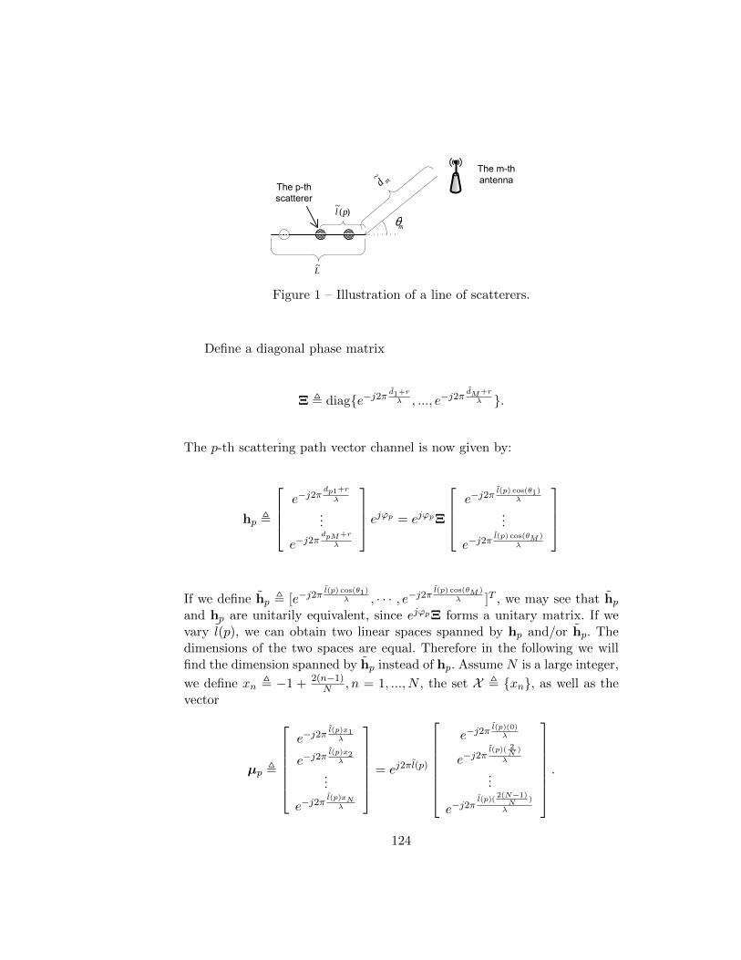
mθ
The m-th antenna
The p-th scatterer
)(~
pl
L~
md~
Figure 1 – Illustration of a line of scatterers.
Define a diagonal phase matrix
Ξ , diag{e−j2πd1+rλ , ..., e−j2π
dM+r
λ }.
The p-th scattering path vector channel is now given by:
hp ,
e−j2π
dp1+r
λ
...
e−j2πdpM+r
λ
ejϕp = ejϕpΞ
e−j2π
l(p) cos(θ1)λ
...
e−j2πl(p) cos(θM )
λ
If we define hp , [e−j2πl(p) cos(θ1)
λ , · · · , e−j2πl(p) cos(θM )
λ ]T , we may see that hpand hp are unitarily equivalent, since ejϕpΞ forms a unitary matrix. If wevary l(p), we can obtain two linear spaces spanned by hp and/or hp. Thedimensions of the two spaces are equal. Therefore in the following we willfind the dimension spanned by hp instead of hp. Assume N is a large integer,
we define xn , −1 + 2(n−1)N , n = 1, ..., N , the set X , {xn}, as well as the
vector
µp ,
e−j2π
l(p)x1λ
e−j2πl(p)x2λ
...
e−j2πl(p)xNλ
= ej2πl(p)
e−j2π
l(p)(0)λ
e−j2πl(p)( 2
N)
λ
...
e−j2πl(p)(
2(N−1)N
)
λ
.
124
Since l(p) ∼ U(0, L), we reuse the result shown in (9):
dim{span{µp, l(p) ∈ [0, L]}}
=4L
Nλ
N
2+ o
(4L
Nλ
N
2
)
=2L
λ+ o(L).
Note that the above result holds when N is arbitrarily large. We againobserve that when N → ∞, any cos(θm) will fall into the set X , whichindicates
dim{span{hp, l(p) ∈ [0, L]}} ≤ 2L
λ+ o(L). (10)
Recall that the covariance matrix R = E{ 1P
P∑p=1
P∑q=1
hphHq }. Because of the
random and independent phases ϕp and ϕq,
∀p 6= q,E{hphHq } = 0.
R = E{ 1
P
P∑p=1
hphHp } = E{hphHp }.
We can see that the number of scatterers has no impact on the rank ofchannel covariance matrix. Hence according to (10), the rank of R is upperbounded by
rank(R) ≤ 2L
λ+ o(L).
Returning to the one-ring model, we can interpret the ring as the sum oflines, with the total length 2πr. An extreme case is when all of the channelscorresponding to different pieces of the ring span orthogonal spaces, i.e., therank of the covariance matrix is the sum of the spatial dimensions corre-sponding to every pieces of the ring. This is the case when the covariancerank is maximized. Therefore the rank is upper bounded by:
rank(R) ≤ 4πr
λ+ o(r).
Thus Theorem 2 is proven.
125

.6 Proof of Lemma 2:
Proof: Take an angle Φ /∈ [θmini , θmax
i ] and define
u ,a(Φ)√M.
Then we have
uHRiu =1
Ma(Φ)HRia(Φ)
=1
MaH(Φ)E
{a(θ)aH(θ)
}a(Φ)
=1
ME{∣∣aH(Φ)a(θ)
∣∣2}=
1
ME
∣∣∣∣∣M−1∑m=0
e2πj(m−1)Dλ
(cos(Φ)−cos(θ))
∣∣∣∣∣2
=
∫ θmaxi
θmini
1
M
∣∣∣∣∣M−1∑m=0
e2πj(m−1)Dλ
(cos(Φ)−cos(θ))
∣∣∣∣∣2
pi(θ)dθ.
According to the well-known result on the sum of geometric series, we caneasily obtain
limM→∞
1
M
∣∣∣∣∣M−1∑m=0
e2πj(m−1)Dλ
(cos(Φ)−cos(θ))
∣∣∣∣∣2
= 0,
since Φ 6= θ,∀θ ∈ [θmini , θmax
i ]. Thus
limM→∞
uHRiu = 0,
which proves Lemma 2.
126

.7 Proof of Proposition 5:
Proof: Denote the associated path loss as β. The covariance R is a Toeplitzmatrix, with its mn-th entry given by
R(m,n) = β
∫ π
0p(θ)ej2π
Dλ
(n−m) cos(θ)dθ (11)
= β
∫ 1
−1p (arccos(x)) ej2π
Dλ
(n−m)x 1√1− x2
dx
=βλ
2πD
∫ 2πDλ
− 2πDλ
p(arccos( λx
2πD ))√
1−(λx
2πD
)2 ej(n−m)xdx,
=1
2π
∫ 2πDλ
− 2πDλ
f(x)ej(n−m)xdx, (12)
where
f(x) ,βλ
D
p(arccos( λx
2πD ))√
1−(λx
2πD
)2 . (13)
Since 0, π /∈ Φ, or in other words, p(0) = p(π) = 0, and that p(θ) <∞, ∀θ ∈Φ, it follows that f(x) is uniformly bounded:
f(x) < +∞,−2πD
λ≤ x ≤ 2πD
λ. (14)
Thus, the Toeplitz matrix R is related to the real integrable and uniformlybounded generating function f(x), with its entries being Fourier coefficientsof f(x). We now resort to the known result on the spectrum of the n × nToeplitz matrices Tn(f) defined by the generating function f(x). Denote byess inf and ess sup the essential minimum and the essential maximum of f ,i.e., the infimum and the supremum of f up to within a set of measure zero.Let mf , ess inff and Mf , ess supf .
Theorem 8. [95] If λ(n)0 ≤ λ
(n)1 ≤ · · · ≤ λ
(n−1)n−1 are the eigenvalues of
Tn(f), then, the spectrum of Tn(f) is contained in (mf ,Mf ); moreover
limn→∞
λ(n)0 = mf and lim
n→∞λ
(n−1)n−1 = Mf .
By invoking Theorem 8, we obtain that limM→∞
‖R‖2 = Mf < ∞. In
addition, for any finite M , the inequality ‖R‖2 <∞ always holds true. Thisconcludes the proof.
127

.8 Proof of Lemma 4:
Proof: Since Rj and(∑L
l=1 Rl + σ2nIM
)−1are both positive semi-definite
(PSD) Hermitian matrices, we can directly apply the inequalities of [96] onthe eigenvalues of the product of two PSD Hermitian matrices:
‖Ξj‖2 ≤
∥∥∥∥∥∥(
L∑l=1
Rl + σ2nIM
)−1∥∥∥∥∥∥
2
‖Rj‖2 <ζ
σ2n
. (15)
It is straightforward to show that
∥∥ΞjΞHj
∥∥2
= ‖Ξj‖22 <ζ2
σ4n
, (16)
which indicates that the spectral norm of ΞjΞHj is also uniformly bounded.
This proves Lemma 4.
.9 Proof of Lemma 6:
Proof: Using the spatial correlation model (6.6), we may write
1
MhHj hl =
1
MhHWjR
12j ΞH
j ΞjR12l hWl. (17)
By an abuse of notation, we now use the operator λ1{·} to represent thelargest singular value of a matrix. Appealing to the singular value inequalities
in [97], we can show that the maximum singular value of R12j ΞH
j ΞjR12l yields:
λ1{R12j ΞH
j ΞjR12l } ≤ λ1{R
12j }λ1{ΞH
j ΞjR12l } (18)
< ζ12λ1{ΞH
j Ξj}λ1{R12l } (19)
<ζ3
σ4n
, (20)
which means the spectral radius of the complex matrix R12j ΞH
j ΞjR12l is uni-
formly bounded for any M . Thus, according to Lemma 5, 1MhHj hl,∀l 6= j,
converges almost surely to zero. Thus (5.28) holds true. In a similar way, wecan prove (5.29). This concludes the proof of Lemma 6.
128

.10 Proof of Lemma 7:
Proof: Define
Γ , limC→∞
(1
CWjW
Hj
)(21)
= hjhHj +
∑l 6=j
hlhHl + σ2
nΞjΞHj . (22)
In this proof, we first consider the noise free scenario and let
Γnf = hjhHj +
∑l 6=j
hlhHl , (23)
where the subscript “nf” denotes noise free. We can then write
limM→∞
∥∥∥∥∥Γnf
M
hj∥∥hj∥∥2
− αjhj∥∥hj∥∥2
∥∥∥∥∥2
2
(24)
= limM→∞
(Γnf
M
hj∥∥hj∥∥2
− αjhj∥∥hj∥∥2
)H(Γnf
M
hj∥∥hj∥∥2
− αjhj∥∥hj∥∥2
)
= limM→∞
1
M2
∥∥hj∥∥2
2− limM→∞
2αjM
∥∥hj∥∥2
2+ α2
j
= α2j − 2α2
j + α2j
= 0,
Which proves that when M → ∞, an eigenvalue of the random matrixΓnf/M converges to αj , with its corresponding eigenvector converging tohj/∥∥hj∥∥2
up to a random phase.
Then we consider the Hermitian matrix σ2nΞjΞ
Hj as a perturbation on
Γnf/M . Due to the Bauer-Fike Theorem [98] on the perturbation of eigenval-ues of Hermitian matrices, together with Lemma 4, we have for 1 ≤ i ≤ L:
limM→∞
∣∣∣∣λi{ Γ
M
}− λi
{Γnf
M
}∣∣∣∣ (25)
≤ limM→∞
σ2n
M
∥∥ΞjΞHj
∥∥2
(26)
= 0. (27)
The above result shows that the impact of the perturbation on the eigenval-ues of Γnf/M vanishes as M →∞. In other words, αj is again an asymptotic
129

eigenvalue of Γ/M . Now we verify that despite the perturbation, the eigen-vector of Γ/M corresponding to the asymptotic eigenvalue αj also convergesto hj/
∥∥hj∥∥2up to a random phase. To prove this, it is sufficient to show
that
limM→∞
∥∥∥∥∥ Γ
M
hj∥∥hj∥∥2
− αjhj∥∥hj∥∥2
∥∥∥∥∥2
(28)
≤ limM→∞
∥∥∥∥∥Γnf
M
hj∥∥hj∥∥2
− αjhj∥∥hj∥∥2
∥∥∥∥∥2
+
∥∥∥∥∥σ2nΞjΞ
Hj
M
hj∥∥hj∥∥2
∥∥∥∥∥2
(a)= 0,
where (a) is due to the definition of the spectral norm:
limM→∞
∥∥∥∥∥σ2nΞjΞ
Hj
M
hj∥∥hj∥∥2
∥∥∥∥∥2
= 0. (29)
It follows that
limM,C→∞
∥∥∥∥∥WjWHj
MC
hj∥∥hj∥∥2
− αjhj∥∥hj∥∥2
∥∥∥∥∥2
= 0, (30)
which concludes the proof of Lemma 7.
.11 Proof of Lemma 8:
Proof: We can derive:
limM,C→∞
∥∥∥∥∥∥ Ξ′jhj∥∥∥Ξ′jhj∥∥∥2
−Ξ′juj1e
jφ∥∥∥Ξ′juj1∥∥∥2
∥∥∥∥∥∥2
2
(31)
= limM,C→∞
Ξ′jhj∥∥∥Ξ′jhj∥∥∥2
−Ξ′juj1e
jφ∥∥∥Ξ′juj1∥∥∥2
H
·
Ξ′jhj∥∥∥Ξ′jhj∥∥∥2
−Ξ′juj1e
jφ∥∥∥Ξ′juj1∥∥∥2
= 2− lim
M,C→∞
hHj Ξ′jHΞ′juj1e
jφ∥∥∥Ξ′jhj∥∥∥2
∥∥∥Ξ′juj1∥∥∥2
+e−jφuHj1Ξ
′jHΞ′jhj∥∥∥Ξ′jhj∥∥∥
2
∥∥∥Ξ′juj1∥∥∥2
130

We treat the following quantity separately:
limM,C→∞
hHj Ξ′jHΞ′juj1e
jφ∥∥∥Ξ′jhj∥∥∥2
∥∥∥Ξ′juj1∥∥∥2
(32)
= limM,C→∞
hHj Ξ′jHΞ′j
(hj
‖hj‖2+ uj1e
jφ − hj
‖hj‖2
)∥∥∥Ξ′jhj∥∥∥
2
∥∥∥Ξ′juj1∥∥∥2
= limM,C→∞
∥∥∥∥Ξ′j hj
‖hj‖2
∥∥∥∥2∥∥∥Ξ′juj1∥∥∥
2
= limM,C→∞
∥∥∥∥Ξ′j ( hj
‖hj‖2− uj1e
jφ + uj1ejφ
)∥∥∥∥2∥∥∥Ξ′juj1∥∥∥
2
≤ limM,C→∞
∥∥∥∥Ξ′j( hj
‖hj‖2− uj1e
jφ)
∥∥∥∥2∥∥∥Ξ′juj1∥∥∥
2
+ limM,C→∞
∥∥∥Ξ′juj1ejφ∥∥∥2∥∥∥Ξ′juj1∥∥∥
2
= 1 (33)
In a similar way, we can prove that
limM,C→∞
∥∥∥Ξ′juj1∥∥∥2∥∥∥∥Ξ′j hj
‖hj‖2
∥∥∥∥2
≤ 1. (34)
Combining (33) and (34), we obtain:
limM,C→∞
hHj Ξ′jHΞ′juj1e
jφ∥∥∥Ξ′jhj∥∥∥2
∥∥∥Ξ′juj1∥∥∥2
= 1. (35)
With analogous derivation, we can prove
limM,C→∞
e−jφuHj1Ξ′jHΞ′jhj∥∥∥Ξ′jhj∥∥∥
2
∥∥∥Ξ′juj1∥∥∥2
= 1. (36)
131

Applying (35) and (36) to (31) gives:
limM,C→∞
∥∥∥∥∥∥ Ξ′jhj∥∥∥Ξ′jhj∥∥∥2
−Ξ′juj1e
jφ∥∥∥Ξ′juj1∥∥∥2
∥∥∥∥∥∥2
2
= 0. (37)
The following equality holds:
Ξ′jhj = Ξ′jΞjhj = R†jRjhj = hj , (38)
proving that
limM,C→∞
∥∥∥∥ hj‖hj‖2
− uj1ejφ
∥∥∥∥2
= 0, (39)
which completes the proof of Lemma 8.
.12 Proof of Theorem 4:
Proof: From (5.33) we readily obtain
limM,C→∞
hHj uj1
‖hj‖2= 1. (40)
Recall from the uplink training (5.3), we have
hCAj =
1
τuj1u
Hj1
hjsT +
∑l 6=j
hlsT + N
s∗, (41)
132

and hence
limM,C→∞
∥∥∥hCAj − hj
∥∥∥2
2
‖hj‖22(42)
= limM,C→∞
(hCAj − hj)
H(hCAj − hj)
‖hj‖22
= limM,C→∞
1
‖hj‖22
∑l 6=j
hluj1uHj1
∑l 6=j
hl +∑l 6=j
hluj1uHj1N
s∗
τ
+sT
τNH uj1u
Hj1
∑l 6=j
hl +sT
τNH uj1u
Hj1N
s∗
τ
− hHj uj1uHj1hj + hHj hj
)= lim
M,C→∞
1
‖hj‖22
(hHj hj − hHj uj1u
Hj1hj
). (43)
Equation (40) ensures that
limM,C→∞
1
‖hj‖22hHj uj1u
Hj1hj =
1
‖hj‖22hHj hj = 1, (44)
which concludes the proof.
.13 Proof of Theorem 5:
Proof: This proof follows similar steps towards Theorem 4. Thus we givea sketch of the proof only. Define
Γ , limC→∞
(1
CWjW
Hj
)(45)
= h(j)j h
(j)Hj +
∑l 6=j
h(j)l h
(j)Hl + σ2
nΞjΞHj , (46)
where h(j)l , Ξjh
(j)l , l = 1, . . . , L. Due to the asymptotic orthogonality
between steering vectors in disjoint angular support, i.e., Lemma 3 in [36],
we can easily show that in large antenna limit, h(j)lo falls into the null space
of R(j)j . Thus
limM→∞
1
Mh
(j)l h
(j)Hl = lim
M→∞
1
Mh
(j)li h
(j)Hli . (47)
133

Then we have
limM→∞
Γ
M=
1
M
h(j)j h
(j)Hj +
∑l 6=j
h(j)li h
(j)Hli + σ2
nΞjΞHj
.
Under condition C1, it is easy to show that
limM→∞
∥∥∥∥∥∥ Γ
M
h(j)j∥∥∥h(j)j
∥∥∥2
−h
(j)H
j h(j)j
M
h(j)j∥∥∥h(j)j
∥∥∥2
∥∥∥∥∥∥2
= 0. (48)
Given the following condition
∀l 6= j,∥∥∥Ξjh
(j)li
∥∥∥2<∥∥∥Ξjh
(j)j
∥∥∥2, (49)
it is clear that the dominant eigenvector of Γ/M converges to h(j)j /∥∥∥h(j)
j
∥∥∥2
(up to a random phase), with its corresponding eigenvalue converging to
h(j)H
j h(j)j /M . Then, using the same technique in the proof of Lemma 8, we
obtain:
limM,C→∞
h(j)H
j uj1∥∥∥h(j)j
∥∥∥2
= 1. (50)
Finally, we readily obtain (5.39) by analogous derivations in Appendix .12.
134

Bibliography
[1] A. F. Molisch, Wireless communications. Wiley, 2010.
[2] W. C. Jakes, Mobile microwave communication. Wiley, 1974.
[3] D. S. Shiu, G. J. Foschini, M. J. Gans, and J. M. Kahn, “Fading corre-lation and its effect on the capacity of multielement antenna systems,”IEEE Trans. Commun., vol. 48, no. 3, pp. 502–513, Mar. 2000.
[4] H. Yin, L. Cottatellucci, D. Gesbert, R. Muller, and G. He, “Robustpilot decontamination based on joint angle and power domaindiscrimination,” Submitted to IEEE Trans. Signal Process., 2015.[Online]. Available: http://arxiv.org/abs/1509.06024
[5] N. Jindal, “MIMO broadcast channels with finite-rate feedback,” IEEETrans. Inf. Theory, vol. 52, no. 11, pp. 5045–5060, 2006.
[6] H. Yin, L. Cottatellucci, and D. Gesbert, “Enabling massive MIMOsystems in the FDD mode thanks to D2D communications,” in Proc. ofAsilomar Conference on Signals, Systems, and Computers, PacificGrove, CA, Nov 2014, pp. 656–660.
[7] A. Gorokhov, “Antenna selection algorithms for MEA transmission sys-tems,” in 2002 IEEE International Conference on Acoustics, Speech,and Signal Processing (ICASSP), vol. 3, Orlando, FL, USA, May 2002,pp. III–2857–III–2860.
[8] A. Gorokhov, D. A. Gore, and A. J. Paulraj, “Receive antenna selectionfor MIMO spatial multiplexing: theory and algorithms,” IEEE TransSignal Process., vol. 51, no. 11, pp. 2796–2807, 2003.
[9] A. Lozano, R. W. Heath, and J. G. Andrews, “Fundamental limits ofcooperation,” IEEE Trans. Inf. Theory, vol. 59, no. 9, pp. 5213–5226,2013.
[10] T. L. Marzetta, “Noncooperative cellular wireless with unlimited num-bers of base station antennas,” IEEE Trans. Wireless Commun, vol. 9,no. 11, pp. 3590–3600, Nov. 2010.
135

[11] F. Rusek, D. Persson, B. K. Lau, E. G. Larsson, T. L. Marzetta, O. Ed-fors, and F. Tufvesson, “Scaling up MIMO: Opportunities and chal-lenges with very large arrays,” IEEE Signal Process. Mag., vol. 30, no. 1,pp. 40–60, 2013.
[12] J. Hoydis, S. ten Brink, and M. Debbah,“Massive MIMO in the UL/DLof cellular networks: How many antennas do we need?” IEEE J. Sel.Areas Commun., vol. 31, no. 2, pp. 160–171, 2013.
[13] E. G. Larsson, F. Tufvesson, O. Edfors, and T. L. Marzetta, “MassiveMIMO for next generation wireless systems,” IEEE Commun. Mag.,vol. 52, no. 2, pp. 186–195, Feb. 2014.
[14] J. Jose, A. Ashikhmin, T. L. Marzetta, and S. Vishwanath, “Pilot con-tamination problem in multi-cell TDD systems,” in Proc. IEEE Inter-national Symposium on Information Theory (ISIT’09), Seoul, Korea,Jun. 2009, pp. 2184–2188.
[15] J. Hoydis, S. ten Brink, and M. Debbah, “Massive MIMO: How manyantennas do we need?” in Proc. 2011 49th Annual Allerton Conferenceon Communication, Control, and Computing (Allerton), Sep. 2011, pp.545 –550.
[16] J. Jose, A. Ashikhmin, T. L. Marzetta, and S. Vishwanath, “Pilot con-tamination and precoding in multi-cell TDD systems,” IEEE Trans.Wireless Commun., vol. 10, no. 8, pp. 2640–2651, Aug. 2011.
[17] A. Adhikary, J. Nam, J.-Y. Ahn, and G. Caire, “Joint spatial divisionand multiplexing – the large-scale array regime,” IEEE Trans. Inf. The-ory, vol. 59, no. 10, pp. 6441–6463, Oct 2013.
[18] E. Bjornson, E. G. Larsson, and T. L. Marzetta, “Massive MIMO: 10myths and one grand question,” To appear in IEEE CommunicationsMagazine, 2015. [Online]. Available: http://arxiv.org/abs/1503.06854
[19] R. Rogalin, O. Y. Bursalioglu, H. Papadopoulos, G. Caire, A. F.Molisch, A. Michaloliakos, V. Balan, and K. Psounis, “Scalable synchro-nization and reciprocity calibration for distributed multiuser MIMO,”IEEE Trans. Wireless Commun, vol. 13, no. 4, pp. 1815–1831, 2014.
[20] E. Bjornson, J. Hoydis, M. Kountouris, and M. Debbah, “MassiveMIMO systems with non-ideal hardware: energy efficiency, estimation,and capacity limits,” Submitted to IEEE Trans. Inf. Theory, 2013.[Online]. Available: http://arxiv.org/abs/1307.2584
[21] A. Pitarokoilis, S. K. Mohammed, and E. G. Larsson, “Uplink per-formance of time-reversal MRC in massive MIMO systems subject to
136

phase noise,” IEEE Trans. Wireless Commun, vol. 14, no. 2, pp. 711–723, 2015.
[22] H. Q. Ngo, T. L. Marzetta, and E. G. Larsson, “Analysis of the pilotcontamination effect in very large multicell multiuser MIMO systems forphysical channel models,” in Proc. IEEE International Conference onAcoustics, Speech and Signal Processing (ICASSP2011), Prague, CzechRepublic, May 2011, pp. 3464–3467.
[23] B. Gopalakrishnan and N. Jindal, “An analysis of pilot contaminationon multi-user MIMO cellular systems with many antennas,” in 2011IEEE 12th International Workshop on Signal Processing Advances inWireless Communications (SPAWC), Jun. 2011, pp. 381–385.
[24] K. Appaiah, A. Ashikhmin, and T. L. Marzetta, “Pilot contaminationreduction in multi-user TDD systems,” in 2010 IEEE InternationalConference on Communications (ICC), Cape Town, South Africa, May2010, pp. 1–5.
[25] F. Fernandes, A. Ashikhmin, and T. L. Marzetta, “Inter-cell interfer-ence in noncooperative TDD large scale antenna systems,” IEEE J. Sel.Areas Commun., vol. 31, no. 2, pp. 192–201, 2013.
[26] A. Ashikhmin and T. Marzetta, “Pilot contamination precoding inmulti-cell large scale antenna systems,” in IEEE International Sym-posium on Information Theory Proceedings (ISIT2012). Cambridge,MA, USA: IEEE, 2012, pp. 1137–1141.
[27] H. Q. Ngo and E. G. Larsson, “EVD-based channel estimation in multi-cell multiuser MIMO systems with very large antenna arrays,” in Proc.IEEE International Conference on Acoustics, Speech, and Signal Pro-cessing (ICASSP). IEEE, 2012, pp. 3249–3252.
[28] R. R. Muller, L. Cottatellucci, and M. Vehkapera, “Blind pilot decon-tamination,” IEEE J. Sel. Topics Signal Process, vol. 8, no. 5, pp. 773–786, Oct. 2014.
[29] L. Cottatellucci, R. R. Muller, and M. Vehkapera, “Analysis of pilotdecontamination based on power control,” in Proc. of IEEE VehicularTechnology Conference (VTC), Jun 2013, pp. 1–5.
[30] D. Neumann, M. Joham, and W. Utschick, “Suppression of pilot-contamination in massive MIMO systems,” in IEEE InternationalWorkshop on Signal Processing Advances in Wireless Communications(SPAWC2014). IEEE, Jun. 2014, pp. 11–15.
[31] ——, “Channel estimation in massive MIMO systems,” arXiv preprint,2015. [Online]. Available: http://arxiv.org/abs/1503.08691
137

[32] J. H. Sørensen and E. D. Carvalho, “Pilot decontamination throughpilot sequence hopping in massive MIMO systems,” in Proc. of IEEEGlobal Telecommunications Conference (Globecom), Dec. 2014, pp. 1–6.
[33] I. Atzeni, J. Arnau, and M. Debbah, “Fractional pilot reuse in massiveMIMO systems.” [Online]. Available: http://arxiv.org/abs/1503.07321
[34] D. Hu, L. He, and X. Wang, “Semi-blind pilot decontamination formassive MIMO systems,”IEEE Trans. Wireless Commun., no. 99, Sept.2015.
[35] V. Zarzoso and P. Comon, “Robust independent component analysis byiterative maximization of the kurtosis contrast with algebraic optimalstep size,” IEEE Transactions on Neural Networks, vol. 21, no. 2, pp.248–261, 2010.
[36] H. Yin, D. Gesbert, M. Filippou, and Y. Liu, “A coordinated approachto channel estimation in large-scale multiple-antenna systems,” IEEEJ. Sel. Areas Commun., vol. 31, no. 2, pp. 264–273, Feb. 2013.
[37] D. Neumann, A. Gruendinger, M. Joham, and W. Utschick, “Pilot coor-dination for large-scale multi-cell TDD systems,” in 18th InternationalITG Workshop on Smart Antennas (WSA), Mar. 2014.
[38] J. Chen and V. K. N. Lau, “Two-tier precoding for FDD multi-cellmassive MIMO time-varying interference networks,” IEEE J. Sel. AreasCommun., vol. 32, no. 6, pp. 1230–1238, 2014.
[39] J. Choi, Z. Chance, D. J. Love, and U. Madhow, “Noncoherent trelliscoded quantization: A practical limited feedback technique for massiveMIMO systems,” IEEE Trans. Commun., vol. 61, no. 12, pp. 5016–5029,2013.
[40] B. Lee, J. Choi, J.-Y. Seol, D. J. Love, and B. Shim, “Antenna group-ing based feedback reduction for FDD-based massive MIMO systems,”in IEEE International Conference on Communications (ICC), Sydney,Australia, Jun. 2014, pp. 4477–4482.
[41] B. Lee, J. Choi, J.-y. Seol, D. J. Love, and B. Shim, “Antenna groupingbased feedback compression for FDD-based massive MIMO systems,”To appear in IEEE Trans. Commun., 2015. [Online]. Available:http://arxiv.org/abs/1408.6009
[42] S. T. Qaseem and T. Y. Al-Naffouri, “Compressive sensing for reducingfeedback in MIMO broadcast channels,” in IEEE International Confer-ence on Communications (ICC), Cape Town, South Africa, 2010, pp.1–5.
138

[43] C. Qi and L. Wu, “A hybrid compressed sensing algorithm for sparsechannel estimation in MIMO OFDM systems,” in IEEE InternationalConference on Acoustics, Speech and Signal Processing (ICASSP),Prague, Czech Republic, May 2011, pp. 3488–3491.
[44] P.-H. Kuo, H. Kung, and P.-A. Ting, “Compressive sensing basedchannel feedback protocols for spatially-correlated massive antenna ar-rays,” in IEEE Wireless Communications and Networking Conference(WCNC), Paris, France, Apr. 2012, pp. 492–497.
[45] S. L. H. Nguyen and A. Ghrayeb, “Compressive sensing-based chan-nel estimation for massive multiuser mimo systems,” in IEEE Wire-less Communications and Networking Conference (WCNC), Shanghai,China, Apr. 2013, pp. 2890–2895.
[46] Z. Gao, L. Dai, and Z. Wang,“Structured compressive sensing based su-perimposed pilot design in downlink large-scale MIMO systems,” Elec-tronics Letters, vol. 50, no. 12, pp. 896–898, 2014.
[47] M. E. Eltayeb, T. Al-Naffouri, and H. Bahrami, “Compressive sens-ing for feedback reduction in MIMO broadcast channels,” IEEE Trans.Commun., vol. 62, no. 9, pp. 3209–3222, Sept. 2014.
[48] M. Masood, L. H. Afify, and T. Y. Al-Naffouri, “Efficient coordinatedrecovery of sparse channels in massive MIMO,” IEEE Trans Signal Pro-cess., vol. 63, no. 1, pp. 104–118, 2015.
[49] W. Shen, B. Wang, J. Feng, C. Gao, and J. Ma, “Differential CSITacquisition based on compressive sensing for FDD massive MIMO sys-tems,” in IEEE Vehicular Technology Conference (VTC Spring), Glas-gow, U.K., May 2015, pp. 1–4.
[50] D. L. Donoho, “Compressed sensing,” IEEE Trans. Inf. Theory, vol. 52,no. 4, pp. 1289–1306, 2006.
[51] E. J. Candes, J. Romberg, and T. Tao, “Robust uncertainty principles:exact signal reconstruction from highly incomplete frequency informa-tion,” IEEE Trans. Inf. Theory, vol. 52, no. 2, pp. 489–509, 2006.
[52] E. J. Candes, J. K. Romberg, and T. Tao, “Stable signal recovery fromincomplete and inaccurate measurements,” Communications on pureand applied mathematics, vol. 59, no. 8, pp. 1207–1223, 2006.
[53] E. J. Cande and M. B. Wakin, “An introduction to compressive sam-pling,” IEEE Signal Processing Magazine, vol. 25, no. 2, pp. 21–30,2008.
139

[54] W. U. Bajwa, J. Haupt, A. M. Sayeed, and R. Nowak, “Compressedchannel sensing: A new approach to estimating sparse multipath chan-nels,” Proceedings of the IEEE, vol. 98, no. 6, pp. 1058–1076, 2010.
[55] Y.-D. Lin and Y.-C. Hsu, “Multihop cellular: A new architecture forwireless communications,” in Nineteenth Annual Joint Conference ofthe IEEE Computer and Communications Societies (IEEE INFOCOM2000), vol. 3, 2000, pp. 1273–1282.
[56] B. Kaufman and B. Aazhang,“Cellular networks with an overlaid deviceto device network,” in 2008 Asilomar Conference on Signals, Systemsand Computers, Pacific Grove, CA, USA, Oct 2008, pp. 1537–1541.
[57] K. Doppler, M. Rinne, C. Wijting, C. B. Ribeiro, and K. Hugl, “Device-to-device communication as an underlay to LTE-advanced networks,”IEEE Communications Magazine, vol. 47, no. 12, pp. 42–49, 2009.
[58] K. Doppler, M. P. Rinne, P. Janis, C. Ribeiro, and K. Hugl, “Device-to-Device communications; functional prospects for LTE-advanced net-works,” in IEEE International Conference on Communications Work-shops (ICC Workshops 2009), Dresden, Germany, Jun. 2009, pp. 1–6.
[59] T. Peng, Q. Lu, H. Wang, S. Xu, and W. Wang, “Interference avoid-ance mechanisms in the hybrid cellular and device-to-device systems,”in IEEE International Symposium on Personal, Indoor and Mobile Ra-dio Communications (PIMRC), Jun. 2009, pp. 617–621.
[60] J. Du, W. Zhu, J. Xu, Z. Li, and H. Wang, “A compressed HARQfeedback for device-to-device multicast communications,” in IEEE Ve-hicular Technology Conference (VTC Fall), Quebec City, Canada, Sept.2012, pp. 1–5.
[61] B. Zhou, H. Hu, S.-Q. Huang, and H.-H. Chen, “Intracluster device-to-device relay algorithm with optimal resource utilization,” IEEE Trans.Veh. Technol., vol. 62, no. 5, pp. 2315–2326, 2013.
[62] N. Golrezaei, A. G. Dimakis, and A. F. Molisch, “Device-to-device col-laboration through distributed storage,” in IEEE Global Communica-tions Conference (GLOBECOM), Anaheim, CA, USA, Dec. 2012, pp.2397–2402.
[63] J. C. Li, M. Lei, and F. Gao, “Device-to-device (d2d) communication inmu-mimo cellular networks,” in IEEE Global Communications Confer-ence (GLOBECOM), Anaheim, CA, USA, Dec. 2012, pp. 3583–3587.
[64] N. Golrezaei, P. Mansourifard, A. F. Molisch, and A. G. Dimakis,“Base-station assisted device-to-device communications for high-throughput
140

wireless video networks,” IEEE Trans. Wireless Commun., vol. 13,no. 7, pp. 3665–3676, 2014.
[65] L. Lei, Z. Zhong, C. Lin, and X. Shen, “Operator controlled device-to-device communications in LTE-advanced networks,” IEEE WirelessCommunications, vol. 19, no. 3, p. 96, 2012.
[66] X. Lin, R. Heath, and J. Andrews.
[67] S. Shalmashi, E. Bjornson, M. Kountouris, K. W. Sung, and M. Debbah,“Energy efficiency and sum rate when massive MIMO meets device-to-device communication,” in IEEE International Conference on Commu-nications (ICC), London, UK, Jun. 2015.
[68] ——, “Energy efficiency and sum rate tradeoffs for massive mimosystems with underlaid device-to-device communications,” Submitted,2015. [Online]. Available: http://arxiv.org/abs/1506.00598
[69] R. B. Ertel, P. Cardieri, K. W. Sowerby, T. S. Rappaport, and J. H.Reed, “Overview of spatial channel models for antenna array commu-nication systems,” IEEE Pers. Commun., vol. 5, no. 1, pp. 10 –22, Feb.1998.
[70] S. Wagner, R. Couillet, M. Debbah, and D. Slock, “Large system anal-ysis of linear precoding in correlated MISO broadcast channels underlimited feedback,” IEEE Trans. Inf. Theory, vol. 58, no. 7, pp. 4509–4537, 2012.
[71] R. Knopp and P. A. Humblet, “Information capacity and power controlin single-cell multiuser communications,” in Proc. IEEE InternationalConference on Communications, vol. 1, Seattle, WA, USA, Jun. 1995,pp. 331–335.
[72] P. Viswanath, D. N. C. Tse, and R. Laroia,“Opportunistic beamformingusing dumb antennas,” IEEE Trans. Inf. Theory, vol. 48, no. 6, pp.1277–1294, Jun. 2002.
[73] J. Jang and K. B. Lee,“Transmit power adaptation for multiuser OFDMsystems,” IEEE J. Sel. Areas Commun., vol. 21, no. 2, pp. 171–178, Feb.2003.
[74] D. Gesbert, M. Kountouris, R. Heath, C. Chae, and T. Salzer, “Shiftingthe MIMO paradigm,” IEEE Signal Process. Mag., vol. 24, no. 5, pp.36–46, Sep. 2007.
[75] A. J. Paulraj, R. Nabar, and D. Gore, Introduction to space-time wire-less communications. Cambridge University Press, 2003.
141

[76] A. Scherb and K. D. Kammeyer, “Bayesian channel estimation for dou-bly correlated MIMO systems,” in Proc. IEEE Workshop Smart Anten-nas, 2007.
[77] E. Bjornson and B. Ottersten, “A framework for training-based estima-tion in arbitrarily correlated Rician MIMO channels with Rician dis-turbance,” IEEE Trans. Signal Process., vol. 58, no. 3, pp. 1807–1820,Mar. 2010.
[78] R. M. Gray and L. D. Davisson, An introduction to statistical signalprocessing. Cambridge University Press, 2004.
[79] S. M. Kay, Fundamentals of Statistical Signal Processing: EstimationTheory. Englewood Cliffs, NJ: Prentice Hall, 1993.
[80] J. A. Fill and D. E. Fishkind, “The Moore–Penrose generalized inversefor sums of matrices,” SIAM Journal on Matrix Analysis and Applica-tions, vol. 21, no. 2, pp. 629–635, 2000.
[81] M. A. Rakha, “On the Moore–Penrose generalized inverse matrix,” Ap-plied Mathematics and Computation, vol. 158, no. 1, pp. 185–200, 2004.
[82] H. Yin, D. Gesbert, and L. Cottatellucci, “Dealing with interference indistributed large-scale MIMO systems: A statistical approach,” IEEEJ. Sel. Topics Signal Process., vol. 8, no. 5, pp. 942–953, Oct. 2014.
[83] A. Adhikary and G. Caire, “Joint spatial division and multiplexing:Opportunistic beamforming and user grouping,” arXiv preprint, 2013.[Online]. Available: http://arxiv.org/abs/1305.7252
[84] J. Evans and D. N. C. Tse, “Large system performance of linear mul-tiuser receivers in multipath fading channels,” IEEE Trans. Inf. Theory,vol. 46, no. 6, pp. 2059–2078, 2000.
[85] H. Yin, L. Cottatellucci, D. Gesbert, R. Muller, and G. He, “Pilot de-contamination using combined angular and amplitude based projectionsin massive MIMO systems,” in IEEE 16th Workshop on Signal Process-ing Advances in Wireless Communications, SPAWC 2015, Stockholm,Sweden, Jun. 2015, pp. 216–220.
[86] T. S. Rappaport, Wireless communications: principles and practice.Prentice Hall PTR New Jersey, 1996, vol. 2.
[87] T. L. Marzetta, “How much training is required for multiuser MIMO?”in Proc. of the Fortieth Asilomar Conf. on Signals, Systems, & Com-puters, Pacific Grove, CA, USA, Oct. 2006.
[88] H. Q. Ngo, E. G. Larsson, and T. L. Marzetta,“Energy and spectral effi-ciency of very large multiuser MIMO systems,” IEEE Trans. Commun.,vol. 61, no. 4, pp. 1436–1449, Apr. 2013.
142

[89] J. Nam, J. Ahn, and G. Caire, “Joint spatial division and multiplex-ing: Realizing massive MIMO gains with limited channel state informa-tion,” in 46th Annual Conference on Information Sciences and Systems,(CISS 2012), Princeton University, NJ, USA, Mar. 2012.
[90] X. Rao, V. K. Lau, and X. Kong, “CSIT estimation and feedback forFDD multi-user massive MIMO systems,” in 2014 IEEE InternationalConference on Acoustics, Speech and Signal Processing (ICASSP),2014, pp. 3157–3161.
[91] X. Rao and V. K. Lau, “Distributed compressive CSIT estimation andfeedback for FDD multi-user massive MIMO systems,” IEEE Trans Sig-nal Process., vol. 62, no. 12, pp. 3261–3271, 2014.
[92] P. Ding, D. J. Love, and M. D. Zoltowski, “Multiple antenna broadcastchannels with shape feedback and limited feedback,” IEEE Trans SignalProcess., vol. 55, no. 7, pp. 3417–3428, 2007.
[93] D. J. Love and R. W. Heath, “Limited feedback unitary precoding forspatial multiplexing systems,” IEEE Trans. Inf. Theory, vol. 51, no. 8,pp. 2967–2976, 2005.
[94] D. J. Love, R. W. Heath, V. K. N. Lau, D. Gesbert, B. D. Rao, andM. Andrews, “An overview of limited feedback in wireless communica-tion systems,” IEEE J. Sel. Areas Commun., vol. 26, no. 8, pp. 1341–1365, Oct. 2008.
[95] U. Grenander and G. Szego, Toeplitz forms and their applications. 2nded. Chelsea, New York, 1984.
[96] A. W. Marshall, I. Olkin, and B. Arnold, Inequalities: theory of ma-jorization and its applications. Springer Science & Business Media,2010.
[97] R. A. Horn and C. R. Johnson, Topics in matrix analysis. CambridgeUniversity Press, 1991.
[98] F. L. Bauer and C. T. Fike, “Norms and exclusion theorems,” Nu-merische Mathematik, vol. 2, no. 1, pp. 137–141, 1960.
143