dissertation numerical modeling of reservoir …
TRANSCRIPT

DISSERTATION
NUMERICAL MODELING OF RESERVOIR SEDIMENTATION AND FLUSHING
PROCESSES
Submitted by
Jungkyu Ahn
Department of Civil and Environmental Engineering
In partial fulfillment of the requirements
For the Degree of Doctor of Philosophy
Colorado State University
Fort Collins, Colorado
Fall 2011
Doctoral Committee:
Advisor: Chih Ted Yang
Pierre Y. Julien
Christopher I. Thornton
Ellen E. Wohl

ii
ABSTRACT
NUMERICAL MODELING OF RESERVOIR SEDIMENTATION AND FLUSHING
PROCESSES
As rivers flow into reservoirs, part of the transported sediment will be deposited.
Sedimentation in the reservoir may significantly reduce reservoir storage capacity.
Reservoir capacity can be recovered by removing deposited sediment by dredging or
flushing. Generally speaking, the latter is preferable to the former. An accurate estimation
sedimentation volume and its removal are required for the development of a long term
operation plan in the design stage.
One-dimensional, 1D, models are more suitable for a long term simulation of
channel cross section change of a long study reach than two or three dimensional models.
A 1D model, GSTARS3, was considered, because this study focuses on sedimentation
and flushing in the entire reservoir over several years and GSTARS3 can predict channel
geometry in a semi-two dimensional manner by using the stream tube concept. However,
like all 1D numerical models, GSTARS3 is based on some simplified assumptions.
iii
One of the major assumptions made for GSTARS3 is steady or quasi-steady flow
condition, which is valid for most reservoir operation. If there is no significant flow
change in a reservoir, such as rapid water surface drop during flushing, steady model can
be applied. However, unsteady effect due to the flushing may not be ignored and should
be considered for the numerical modeling of flushing processes. Not only flow
characteristics but also properties of bed materials in reservoir regime may be different
from those in a river regime. Both reservoir and river regimes should be considered for a
drawdown flushing study. Flow in the upper part of a reservoir may become river flow
during a drawdown flushing operation. A new model, GSTARS4 (Yang and Ahn, 2011)
was developed for reservoir sedimentation and flushing simulations in this study. It has
the capabilities of simulating unsteady flow and coexistence of river and reservoir
regimes in the study area.
GSTARS4 was applied to the Xiaolangdi Reservoir, located on the main stream
of the Yellow River. The sediment concentration in the reservoir is very high, 10 ~ 100
kg/m3 for common operation and 100 ~ 300 kg/m
3 for flushing operation, with very fine
materials about 20 ~ 70 % of clay. Stability criteria for computing sediment transport and
channel geometric changes by using GSTARS4 model was derived and verified for the
Xiaolangdi Reservoir sedimentation and flushing computations.
Han’s (1980) non-equilibrium sediment transport equation and the modified unit
stream power equation for hyper-concentrated sediment flows by Yang et al. (1996) were
used. Both unsteady and quasi-steady simulations were conducted for 3.5 years with
calibrated site-specific coefficients of the Xiaolangdi Reservoir. The computed thalweg
elevation, channel cross section, bed material size, volume of reservoir sedimentation,

iv
and gradation of flushed sediments were compared with the measured results. The
unsteady computation results are closer to the measurements than those of the steady
flow simulation results.

v
ACKNOWLEDGEMENTS
I would like to express my gratitude to Dr. Chih Ted Yang who supported my Ph.D.
study and provided me with valuable suggestions and guidance to improve my
understanding of sediment transport theories and engineering. His advices not only
improved my academic development but also guided me to become a better engineer. It is
a great honor for me to be his student. I also wish to acknowledge the contributions of my
committee members, Dr. Pierre Julien, Dr. Christopher Thornton, and Dr. Ellen Wohl for
their advices to complete my course work and dissertation.
I wish to express my appreciation to fellow civil engineering students at CSU who
encouraged me during my studies. I am grateful to CSU faculty members who provided
the needed academic background in classes.
I am grateful to my parents for their support and encouragement of my Ph.D. studies.

vi
TABLE OF CONTENTS
ABSTRACT …………………………………………………………………………….. ii
ACKNOWLEDGEMENTS …………………………………………………………....... v
TABLE OF CONTENTS ……………………………………………………………….. vi
LIST OF TABLES ………………………………………………………………............. x
LIST OF FIGURES ……………………………………………………………………. xii
LIST OF SYMBOLS …………………………………………………………………... xv
CHAPTER 1. INTRODUCTION ……………………………………………………...... 1
1.1 Overview …………………………………………………………………………... 1
1.2 General Description of Xiaolangdi Reservoir ……………………………………... 1
1.3 Objectives……………………………………………………………….................. 4
1.4 Study Methodology ………………………………………………………………... 5
CHAPTER 2. LITERATURE REVIEW ……………………………………………....... 8
2.1 General Reservoir Sedimentation Process ………………………………………… 8
2.2 Reservoir Sedimentation Control Methods ………………………………………. 10

vii
2.3 Previous Studies of Reservoir Sedimentation and Flushing ……………………... 13
2.4 Numerical Modeling (1D, 2D, and 3D) ………………………………………….. 15
2.5 Previous Numerical Models ……………………………………………………… 16
CHAPTER 3. THEORETICAL BACKGROUND OF GSTARS4 ………………......... 18
3.1 Hydraulic Computation of GSTARS4 …………………………………………… 18
3.1.1 Quasi-steady Flow Computation ……………………………………………... 18
3.1.2 Unsteady Flow Computation .………………………………………………... 20
3.2 Sediment Routing and Channel Adjustment of GSTARS4 ……………………… 24
3.2.1 Governing Equation and Numerical Scheme for Channel Adjustment ……… 24
3.2.2 Sediment Transport Equations ……………………………………………….. 26
3.2.3 Non-equilibrium Sediment Transport ………………………………………... 28
CHAPTER 4. NEW CAPABILITIES OF GSTARS4 …………………………………. 30
4.1 Addition of Unsteady Flow Simulation ………………………………………….. 31
4.2 Revision of Sediment Transport and Channel Adjustment ………………………. 33
4.2.1 Influence of Tributaries ………………………………………………………. 33
4.2.2 Recovery Factor ……………………………………………………………… 37
4.2.3 Variation of Deposited Sediment Density …………………………………… 42
4.2.4 Size Distribution of Incoming Sediment from Upstream Boundary ………… 42
4.2.5 Percentage of Wash Load ……………………………………………………. 44

viii
CHAPTER 5. NUMERICAL STABILITY CRITERIA FOR CHANNEL
ADJUSTMENT ………………………………………………………………………... 45
5.1 Derivation of Kinematic Wave Speed of Bed Change for Steady Flow Simulation …… 45
5.2 Derivation of Kinematic Wave Speed of Bed Change for Unsteady Flow Simulation ... 48
CHAPTER 6. APPLICATION OF GSTARS4 TO XIAOLANGDI RESERVOIR
SEDIMENTATION AND FLUSHING ……………………………………………...... 52
6.1 Xiaolangdi Reservoir Data Analysis ……………………………………………... 52
6.1.1 Hydrograph and Sediment Inflow Data ……………………………………… 52
6.1.2 Sediment Size Distribution Data ……………………………………………... 54
6.1.3 Cross Section Geometry Data ………………………………………………... 61
6.1.4 Water Temperature Data ……………………………………………………... 62
6.1.5 Tributary Volume Data ………………………………………………………. 62
6.2 Determination of Time Step and Distance between Cross Sections ……………... 63
6.3 Calibration of Coefficients ……………………………………………………….. 68
6.3.1 Roughness Coefficient (Manning’s n) ……………………………………….. 68
6.3.2 Recovery Factor ……………………………………………………………… 71
6.4 Xiaolangdi Reservoir Sedimentation and Flushing Simulation Results …………. 73
6.4.1 Thalweg Profile ……………………………………………………………….. 74
6.4.2 Cross Sectional Changes ……………………………………………………… 78

ix
6.4.3 Bed Material Size …………………………………………………………….. 86
6.4.4 Yearly Reservoir Sedimentation ……………………………………………... 89
6.4.5 Gradation of Flushed Sediment ……………………………………………… 92
CHAPTER 7. SUMMARY …………………………………………………………….. 94
7.1 Summary and Conclusions ………………………………………………………. 94
7.2 Contributions …………………………………………………………………….. 97
7.3 Recommendations for Future Studies ……………………………………………. 98
REFERENCES ……………………………………………………………………….... 99
Appendix A Simulated Steady Flow Reservoir Operation Type 1 (Steady_OP1),
Unsteady Flow Reservoir Operation Type 1 (Unsteady_OP1), and
Measured Cross Section Geometry ………………………………….. 108
Appendix B Simulated Steady Flow Reservoir Operation Type 2 (Steady_OP2),
Unsteady Flow Reservoir Operation Type 2 (Unsteady_OP2), and
Measured Cross Section Geometry ……………………………………. 124

x
LIST OF TABLES
Table 3.1 Sediment transport equations used for GSTARS3 and GSTARS4 …………. 26
Table 4.1 Upgraded capabilities of GSTARS4 sediment routing …………………........ 33
Table 4.2 Combination of recovery factors ……………………………………………. 41
Table 6.1 Four types of reservoir operation ……………………………………………. 60
Table 6.2 Initial dry specific mass with respect to operation number …………………. 60
Table 6.3 Water temperature of Xiaolangdi Reservoir (assumed values) ……………... 62
Table 6.4 Water stage and tributary volume relationships …………………………….. 63
Table 6.5 Sediment size group for this study …………………………………………... 72
Table 6.6 (a) Calibration of recovery factor, RMS of thalweg elevation ………………. 72
Table 6.6 (b) Calibration of recovery factor, AGD of thalweg elevation ……………… 73
Table 6.7 Calibrated recovery factor for both scour and deposition …………………… 73
Table 6.8 Four simulations of Xiaolangdi Reservoir from May 2003 to October 2006 …. 74
Table 6.9 (a) RMS of thalweg elevation ……………………………………………….. 75
Table 6.9 (b) AGD of thalweg elevation ………………………………………………. 75
Table 6.10 (a) Averaged RMS of cross section data …………………………………... 85
Table 6.10 (b) Averaged AGD of cross section data …………………………………... 85
Table 6.11 (a) RMS of mean bed material size ………………………………………... 87

xi
Table 6.11 (b) AGD of mean bed material size ………………………………………... 88
Table 6.12 Comparison of measured and simulated sedimentation volume .………….. 91
Table 6.13 Comparison of measured and simulated sedimentation volume …………... 91
xii
LIST OF FIGURES
Figure 1.1 Xiaolangdi Dam (Yellow River Conservancy Press, 2004) …………………. 3
Figure 1.2 Plan views of the Xiaolangdi Reservoir and tributaries ……………………... 4
Figure 2.1 Typical formation of delta in a reservoir (Morris and Fan, 1997) ………….... 9
Figure 2.2 Basic type of deposition (Morris and Fan, 1997) …………………………... 10
Figure 2.3 Longitudinal bed profile of reservoir during flushing ……………………… 12
Figure 2.4 Longitudinal profile of retrogressive erosion from flume tests
(Morris and Fan, 1997) …………………………………………………….. 13
Figure 2.5 Operational rule in Jensanpei Reservoir (Hwang, 1985) …………………… 15
Figure 3.1 Definition of variables (Yang and Simões, 2002) ………………………….. 19
Figure 3.2 Representation of a hydrograph by a series of steps with constant discharge
and finite duration (Yang and Simões, 2002) ……………………………… 20
Figure 4.1 Flow chart of GSTARS4 model ……………………………………………. 32
Figure 4.2 Delineation of volumes to build the capacity table for tributaries
(Yang and Simões, 2002) …………………………………………………... 34
Figure 4.3 Relationship between recovery factor and (a) shear velocity, (b) sediment fall
velocity, and (c) */Usω ……………………………………………………. 39

xiii
Figure 4.4 Comparison between measured and simulated bed profiles, using recovery
factor as a function of time and location …………………………………… 41
Figure 4.5 Measured size distribution of flushed sediment from the Sanmenxia Reservoir ... 43
Figure 6.1 Hydrology and operation data of the Xiaolangdi Reservoir …...….………... 53
Figure 6.2 Sediment load and water surface elevation data ……………………………. 54
Figure 6.3 Bed material size distribution surveyed between 10 ~ 13 June 2002 ………. 56
Figure 6.4 Bed material size distributions in 2004 …………………………………….. 57
Figure 6.5 Surveyed d 50 before flushing in year 2002, 2004, and 2005 ……………… 57
Figure 6.6 Measured thalweg elevation ………………………………………………... 61
Figure 6.7 Comparison of longitudinal profiles using different time steps (∆t = 3, 6, and 10
minutes) …………………………………………………………………….. 64
Figure 6.8 Bed material size profile with steady simulation using 24 and 56 cross sections
………………………………………….............................................. 67
Figure 6.9 Measured d50 along the main reservoir reach in June 2002 ………………… 70
Figure 6.10 Variation of Manning’s n values used for the simulation ………………… 70
Figure 6.11 Comparison of surveyed and simulated thalweg elevations ………………. 76
Figure 6.12 Comparisons between measured and GSTARS4 simulation results, October
2003 ………………………………………………………………………. 81
Figure 6.13 Comparisons between measured and GSTARS4 simulation results, October
2004 ………………………………………………………………………. 82
Figure 6.14 Comparisons between measured and GSTARS4 simulation results,
November 2005 …………………………………………………………… 83

xiv
Figure 6.15 Comparisons between measured and GSTARS4 simulation results, October
2006 ………………………………………………………………………. 84
Figure 6.16 Comparison of goodness-of-fit between Steady_OP2 and measured results
…………………………………………………………………………….. 85
Figure 6.17 Comparison of goodness-of-fit between Unsteady_OP2 and measured results
…………………………………………………………………………...... 85
Figure 6.18 Comparisons of bed material size variations ……………………………… 88
Figure 6.19 Measured and simulated sedimentation volumes …………………………. 91
Figure 6.20 Comparisons of incoming and flushed sediment gradation .……………… 93

xv
LIST OF SYMBOLS
A = cross section area,
dA = ineffective cross sectional area,
b = a site-specific coefficient for the determination of relationship between discharge and
sediment in transport,
kC ,1 = incoming sediment of the kth
sediment size group from the upstream,
esc = computational kinematic wave speed of bed changes with steady flow simulation,
euc = computational kinematic wave speed of bed changes with unsteady flow simulation,
kc = kinematic wave speed of bed changes,
C i = concentration of sediment in transportation at cross section i,
mC = sediment concentration at the mouth of a tributary,
Ct = total sediment concentration,
itC , = sediment transport capacity at cross section i,
vC = suspended sediment concentration by volume, including wash load,
d = sediment particle diameter,
50d = mean bed material size,
d50,c = computed mean bed material size,

xvi
d50,m = measured mean bed material size,
dk = geometric mean diameter of sediment size group k,
eF and wF = variables to determine change of velocity head gradient,
Fr = Froude number,
g = gravitational acceleration,
H = elevation of the energy line above the datum,
h = water surface elevation,
mh = tributary mouth bed elevation,
i = cross section index,
j = time index,
J = total number of data set,
K = total number of size fractions,
iK = conveyance (m3/s) at cross section i,
=k size fraction index,
n = Manning’s roughness coefficient,
iQ = time weighted discharges,
Qs = volumetric sediment discharge,
=isQ , sediment transport rate at cross section i ,
=kisQ ,, computed volumetric sediment discharge for size k at cross section i ,
q = discharge of flow per unit width,
qlat = lateral inflow per unit length of channel,
slq = lateral sediment inflow,

xvii
Sf = friction slope,
T = the flow top width,
t = time,
jt = time step j,
*U = shear velocity,
V = flow velocity,
1v and 2v = coefficients for the determination of volume of a tributary,
Vol = volume of water in a tributary,
VR,c = computed volume of sedimentation,
VR,m = measured volume of sedimentation,
VS = unit stream power,
x = length along the flow direction,
y = water depth,
z = bed elevation,
zc = computed bed elevations,
zm = measured bed elevations in meter,
=α recovery factor,
dα = recovery factor for deposition,
kα = recovery factor of sediment size group k,
sα = recovery factor for scour,
sγ = specific weights of sediment,
mγ = specific weights of sediment-laden flow,

xviii
Q∆ = water discharge from a tributary to the reservoir,
=∆ sQ sediment load from or into a tributary,
t∆ = time step interval,
=∆Vol change of tributary volume due to the change of reservoir elevation in a time step,
x∆ = distance between cross section,
ix∆ = distance between cross section i and i+1,
riverx∆ = distance between cross sections for the river reach,
reservoirx∆ = distance between cross sections for the reservoir reach,
z∆ = change in bed elevation (positive for aggradation, negative for scour),
iδ , iϕ , and iσ = coefficients for the determination of flow area,
ε and ξ = coefficients for the determination of recovery factor,
η = volume of sediment in a unit bed layer volume (one minus porosity),
=ki ,η volume of sediment in a unit bed layer for size k at cross section i,
κ = coefficient for the determination of Manning’s n,
λ = velocity distribution coefficient,
ν = kinematic viscosity of clear water,
mν = kinematic viscosity in a sediment-laden flow,
1Φ , 2Φ , and 3Φ = weighting factors that must satisfy 1321 =Φ+Φ+Φ ,
θ = a weight factor,
ρ = specific density of clear water,
mρ = specific density of sediment laden flow,
sρ = specific density of sediment particles,

xix
ω = sediment particle fall velocities in clear water,
kω = fall velocity of sediment size k, and
mω = particle fall velocity in a sediment-laden flow.
CHAPTER 1. INTRODUCTION
1.1 Overview
The construction of dams and reservoirs can provide flood control, water supply,
recreation, and navigation benefits. One of the significant changes on a river caused by a
dam is the sedimentation in the reservoir. Reservoir sedimentation reduces its storage
capacity and may have upstream and downstream impacts on a river. Therefore,
sedimentation in a reservoir should be considered not only in the design phase but also in
its operation phase. Sedimentation in reservoirs reduces water storage, flood control, and
water supply capacities. The storage can be restored by several methods. The removal of
sediment deposition can be done by dredging or by water flow flushing. In most cases
flushing causes less adverse impacts on the disposal of the sediment. The sedimentation
and sediment flushing in the Xiaolangdi Reservoir, where drawdown flushing was
conducted every year, were used in this study.
1.2 General Description of Xiaolangdi Reservoir
Xiaolangdi Dam is located 40km north of Loyang, in Henan Province, China and is
128.42 km downstream of the Sanmenxia Dam on the main stem of the Yellow River. It

1
is a rock fill dam with inclined core. Its construction began in 1994 and was completed in
2000. The maximum height of the dam is 160 m and the crest length is 1667 m. Figs. 1.1
(a) and (b) show the layout at the dam site. Total storage of the Xiaolangdi Reservoir is
about 13 billion m
3. The drainage basin area is about 7.0×10
5 km
2, and average flow at
the dam site is 1.3×10³
m3/s. Sediment concentration in the reservoir is very high, 10 ~
100 kg/m3 for common operation and up to 100 ~ 300 kg/m
3 during some flushing
operations. The bed material and sediment input from the upstream of the reservoir are
very fine with about 20 ~ 70 % clay. The average annual sediment passage is 1.4×10⁹ m
3.
Sediment deposition in the Xiaolangdi Reservoir is controlled by drawdown flushing
through three low-level outlets, usually between May and September each year. The
flushing operation is shown in Fig. 1.1 (b).
There are more than 40 tributaries flowing into the Xiaolangdi Reservoir. Fig. 1.2 is the
plan view of the Xiaolangdi Reservoir and 12 major tributaries with the approximate
location of the “imaginary” tributary to account for the volume of all the smaller
tributaries.
The study area is between Xiaolangdi Dam and Sanmenxia Dam which is located at
about 120 km upstream. Sediment deposition in the Sanmenxia Reservoir is controlled by
drawdown flushing. The incoming water and sediment from the upstream boundary of
the study area is equal to those discharged from the upstream Sanmenxia Reservoir.
Therefore, water and sediment input from flushing operation of the Sanmenxia Reservoir
should be considered in this study.

2

3
(a) Common operation (no flushing)
(b) Flushing operation
Figure 1.1 Xiaolangdi Dam (Yellow River Conservancy Press, 2004)

4
Figure 1.2 Plan views of the Xiaolangdi Reservoir and tributaries
1.3 Objectives
Evaluation of reservoir sedimentation and flushing processes are required for the
development of an operation plan. Numerical modeling is considered for this study,
which focuses on an entire reservoir over several years. The main objectives of this study
are:
1) Development of a numerical model applicable to reservoir sedimentation and
flushing processes.
2) Derivation of stability criteria for computing channel geometric change by using
the new model and determination of time step and distance between cross sections
for the simulation of the Xiaolangdi Reservoir sedimentation and flushing process.
120 km along the channel
5
3) Analysis of field data from the Xiaolangdi Reservoir to build input data for the
numerical model and calibration of site-specific coefficients of the Xiaolangdi
Reservoir.
4) Verification of the new model by comparisons between computed and field
measurements of thalweg elevation, cross section geometry, bed material size,
volume of sedimentation, and gradation of flushed sediments.
1.4 Study Methodology
Scour, transportation, and deposition of sediments are complicated processes.
Mathematical equations for reservoir sedimentation have been derived based on
simplified assumptions or empirical relationships. Numerical models are used to solve
these equations. If the flow and sedimentation conditions in a reservoir are not far from
those assumed in a numerical model, the numerical model may be applicable. For most
reservoirs, some simplified assumption and empirical relationships are used. However,
under complicated flow conditions, such as drawdown flushing with high sediment
concentration, some commonly used assumptions may not be valid. If a numerical model
is based on steady flow assumption, the model may not be applicable for flushing studies
because sediment flushing is usually done by highly unsteady water surface drop for
drawdown flushing.
In most cases, sediment concentration is not high enough to change physical properties of
water, such as viscosity and density. Sediment transport in rivers is treated as sediment

6
transport in clear water. However, in the case of high concentration of fine materials,
such as those in the Yellow River, more complex special considerations must be made.
Therefore, sedimentation studies for sediment-laden reservoirs or rivers must be carried
out carefully considering high sediment concentration flow mechanism. Yang et al.
(1996) modified Yang’s 1979 unit stream power formula for high-concentration sediment
laden flow in the Yellow river. Yang’s modified formula will be used in this study.
Simões and Yang (2006), Yang and Simões (2008) and Simões and Yang (2008) have
shown that the Generalized Sediment Transport model for Alluvial River Simulation ver.
3.0 (GSTARS3) is suitable for most reservoir scouring and silting studies. GSTARS3 not
only can simulate but can also predict morphologic changes of rivers and reservoirs based
on the stream tube concept and the application of minimum stream power theory (Yang
and Song, 1979). However, some of the simplified assumptions in GSTARS3 should be
modified before they can be applied to reservoir sedimentation and drawdown flushing
studies. A new model, GSTARS4, Generalizes Sediment Transport model for Alluvial
River Simulation ver. 4.0 (Yang and Ahn, 2011), was developed. GSTARS4 is a truly
unsteady model, while GSTARS3 is a quasi-steady flow model. The numerical scheme
for GSTARS4 model is based on Sedimentation and River Hydraulics – One-dimension
(SRH-1D), (Huang and Greimann, 2007). SRH-1D unsteady flow computational scheme
was revised and used for GSTARS4.
Some other revisions were also made for GSTARS4 sediment transport and channel
geometric adjustment routing modules.
7
For most cases, the rate of sediment transport or channel geometric change is not as
significant as that in the Yellow River. For simulations of channel change, time steps of 1
~ 24 hours, and distances between cross sections of 100 ~ 1000 m, are typical for river or
reservoir sedimentation studies. However, typical time step and distance between cross
sections used for most reservoirs may lead to numerical instability in this study, because
the rate of sediment transport and channel bed change in the Yellow River and the
Xiaolangdi Reservoir are very high. In this study, stability criteria for the channel
geometric change were derived and applied for the determination of proper time step and
distance between cross sections for the Xiaolangdi Reservoir sedimentation and flushing
studies.
Field measurements were analyzed. Water surface elevation at the Xiaolangdi Dam and
incoming water from Sanmenxia Reservoir were used as downstream and upstream
boundary conditions, respectively. However, some of required data for the simulation,
such as water temperature and density of bed material, were missing, and assumptions
were made.
Thalweg elevation, channel geometry, size distribution of bed materials, volume of
sedimentation, and gradation of flushed sediment were measured several times between
May 2003 and October 2006. Both unsteady and steady flow simulations using
GSTARS4 were conducted for 3.5 years and the results were compared with surveyed
results. The goodness-of-fit between computed, for steady and unsteady simulations, and
surveyed results was evaluated by statistical parameters in this study.

8
CHAPTER 2. LITERATURE REVIEW
Walling (1984) summarized regional sedimentation rates world wide. Chinese reservoirs
have an average of 22 years of estimated reservoir half-life expectancy, which is the
shortest in the world. The average half-life for North America and Europe is more than
250 years. Compared to North American and European reservoirs, Chinese reservoirs
have a very short life expectancy due to high sediment concentration such as that in the
Yellow River. Prediction of sedimentation and operation for sediment management in
reservoirs are critical for Chinese reservoirs. This section presents a literature review of
reservoir sedimentation and sediment control, focusing on drawdown flushing and
numerical models.
2.1 General Reservoir Sedimentation Process
As a natural stream enters a reservoir, the flow depth increases, the flow velocity
decreases, and friction slope becomes milder. In other words, unit stream power, VS,
decreases in a reservoir. This reduces the sediment transport capacity and causes siltation
to form a delta, as shown in Fig. 2.1. Sediment carried into a reservoir will be deposited,
causing bed aggradation and reduction of storage. The deposition generally begins with
delta formation near the reservoir headwater area. Morris and Fan (1997) divided the
sediment deposition into three zones; topset, foreset, and bottomset, as shown in Fig. 2.1.

9
The topset of the delta consists of relatively coarse materials, while the bottomset is
formed with finer materials. Aggradation in the upstream channel may occur over a long
distance above the reservoir. Fan and Morris (1992a) noted the following basic
characteristics of reservoir deltas:
1. There is an abrupt change between the slope of the topset and foreset deposits.
2. Sediment particles on the topset bed are coarser than those on the foreset bed, and
there is an abrupt change in particle diameter between topset and foreset deposits.
3. The elevation of the transition zone from the topset to the foreset bed depends on
the reservoir operating rule and pool elevation.
Topset bedBottomset bed
Foreset bed
Delta deposit
Original river slope
Succeeding slope
flow
Coarse sediment
Fine sediment
Figure 2.1 Typical formation of delta in a reservoir (Morris and Fan, 1997)
Reservoir sedimentation processes vary with complex conditions over the entire basin
such as watershed sediment production, rate of sediment transport, flood frequency,
geometry of river, sediment properties, land use, dam operation and so forth. Morris and
Fan (1997) classified reservoir sedimentation into four general types, as shown in Fig. 2.2.

10
Delta deposits Tapering deposits
Wedge-shape deposits Uniform deposits
Figure 2.2 Basic type of deposition (Morris and Fan, 1997)
2.2 Reservoir Sedimentation Control Methods
Three strategies can be used to control reservoir sedimentation (Fan and Morris, 1992b).
First, the sediment delivered from the basin can be reduced by erosion control or
upstream traps. This strategy may reduce long term sediment input. However, it cannot
be the solution for already reduced reservoir storage.
Second, dredging can recover the reservoir storage. However, this is not practical, due to
high cost and the environmental consequences.
Third, sediment can be removed by the water flow, a hydraulic method. Fan and Morris
(1992b) classified hydraulic methods used in China to manage reservoir sediment
deposition as:
1. Sediment routing during floods.
2. Venting density current.
3. Emptying and flushing.
4. Drawdown flushing.

11
Sediment flushing reduces the hydraulic detention time of high sediment concentration in
reservoirs. In northern China, 80 ~ 90 % of the annual sediment load carried by rivers is
discharged in July and August, whereas 25 ~ 50 % of the annual runoff occurs in the
same period (Fan and Morris, 1992b). In summer seasons, an increase of discharge from
the reservoirs may reduce the detention time and deposition rate. White (2001)
differentiated flushing from sluicing. Flushing is scouring deposited sediments and
passing the sediment laden flow through the dam, while sluicing is passing sediment
laden water through the reservoir during the flood and it is applicable to silt and clay.
Venting a density current can discharge muddy flow carried by the density current
through low level outlets. This method has been applied to the Sanmenxia Reservoir with
18 ~ 36 % venting efficiency, which is the ratio between in and outflow of silt during a
flood (Fan, 1986).
Emptying and flushing should be used when deposition and erosion cannot be balanced
by flushing. This method has been useful with small reservoirs (Fan and Morris, 1992b).
The drawdown flushing method scours sediment deposition by dropping water surface
elevation to increase flushing efficiency. Flushing can be done with a full drawdown of
the reservoir or with an partial drawdown of the water level. With respect to water
surface elevation, White (2001) presented three stages of flushing, as shown in Fig. 2.3.
Mahmood (1987), White and Bettess (1984) and Atkinson (1996) stated that reservoir
water level should be close to the bed elevation to maximize the flushing efficiency, but
partial drawdown can still increases flow velocities at the head water area where the
reservoir delta has formed. In the case of partial drawdown or no drawdown, high flow
velocities at the outlets are localized. Partial drawdown has been conducted for the
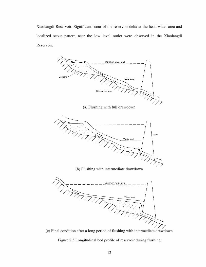
12
Xiaolangdi Reservoir. Significant scour of the reservoir delta at the head water area and
localized scour pattern near the low level outlet were observed in the Xiaolangdi
Reservoir.
(a) Flushing with full drawdown
(b) Flushing with intermediate drawdown
(c) Final condition after a long period of flushing with intermediate drawdown
Figure 2.3 Longitudinal bed profile of reservoir during flushing

13
Fig 2.4 shows the progress of retrogressive erosion (Morris and Fan, 1997). It shows a
zone of high slope and rapid erosion, moving upstream along a channel and having a
lower slope and erosion rate. The maximum erosion rate occurs along the steep slope at
the downstream end of the reservoir delta, causing the maximum erosion area to migrate
upstream through a head cutting process.
Figure 2.4 Longitudinal profile of retrogressive erosion from flume tests
(Morris and Fan, 1997)
2.3 Previous Studies of Reservoir Sedimentation and Flushing
Julien (1998) showed some field measurements of the Tarbela Reservoir in Pakistan. The
life expectancy of that reservoir is about 100 years. Yang and Simões (2002) used
GSTARS3 model to compute the Tarbela Reservoir geometric change over 21 years,
from 1975 to 1996. The simulated bed profile using GSTARS3 is in good agreement with
the measured profile. White (2001) did a similar numerical model study of sedimentation
in the Tarbela Reservoir. His model predicted more deposition than the measurement.

14
Yang and Marsooli (2010) applied GSTARS3 to sedimentation studies of the Ekbatan
Reservoir and Kardeh Reservoir in Iran. The computed bed profiles with calibrated
coefficients are generally in good agreement with the measurements.
Chang et al. (1996) evaluated the efficiency of sediment-pass-through for low level
outlets in reservoirs on the North Fork Feather River using Fluvial-12 (Chang, 1988). The
Fluvial-12 simulation indicated that the sediment-pass-through operation is feasible to
maintain sediment equilibrium for the river/reservoir system, and sediment released from
the reservoir would not have adverse impacts on fish habitat in the river.
Morris and Hu (1992) simulated sediment flushing in the Loíza Reservoir in Puerto Rico
using a one-dimensional model HEC-6 (U.S Army, 1991). The reservoir was assumed as
one-dimensional, because the lateral variation of the channel was not significant.
Flushing with intermediate water surface drawdown has been conducted for the Jensanpei
Reservoir (Hwang, 1985). The storage capacity was reduced due to sedimentation in the
first 15 years of operation. After 15 years of operation, flushing with intermediate water
surface drawdown was conducted once a year, and no further reduction of storage
capacity was observed. The operation rule in a year consists of flushing, refilling, and
deliveries from the storage. With respect to the reservoir operation, water surface changes
are shown in Fig. 2.5. The operation rule applied in the Jensanpei Reservoir is similar to
that of the Xiaolangdi Reservoir.

15
Figure 2.5 Operation rule in Jensanpei Reservoir (Hwang, 1985)
White (2001) summarized 22 case studies of flushing based on field measurements. Most
of them were successful, but some of them were not successful due to downstream
constraints. Morris and Fan (1997) indicated some limitations of flushing. First, there
should be sufficient water to be used for flushing. Second, flushing causes a sudden
release of higher sediment concentration than occurs naturally in the river. High sediment
concentration may create unacceptable downstream impacts, such as clogging of channel
due to deposition and damaging fish habitat.
2.4 Numerical Modeling (1D, 2D, and 3D)
Numerical models are classified as one-dimensional (1D), two-dimensional (2D), and
three-dimensional (3D) models. Most numerical modeling uses a 1D model, which is
more robust than 2D and 3D models (Morris and Fan 1997). White (2001), and Molinas
and Yang (1986) noted that a 1D model is suitable for long-term simulation of reservoir
sedimentation, while 2D or 3D models require much more field data for calibration.
Complicated 2D and 3D models can be used to assess localized impact of flushing near a

16
low level outlet. Generally speaking, a 1D model is suitable for long-term simulation of a
long reach of river or reservoir with elongated channel geometry. 1D model requires the
least amount of data for calibration and verification and their numerical solutions are
relatively simple and stable. 2D or 3D models are suitable for short-term simulations of
localized phenomena of a short reach of a river or reservoir. 2D or 3D models require
large amounts of data for calibration and verification, and their numerical solutions are
complex. Yang (2010) suggested that a quasai-2D model for hydraulic simulation and
prediction and a qusai-3D simulation and prediction of channel geometry and profile
adjustment is more suitable for long-term simulation and prediction of morphologic
changes of a long reach of a river and reservoir with limited field data for engineering
purposes.
2.5 Previous Numerical Models
Most commonly used numerical sediment transport models were originally developed for
movable bed rivers (Morris and Fan 1997). Two numerical models are considered in this
study.
GSTARS3 is a numerical model for simulating the flow of water and sediment transport
in alluvial rivers and reservoirs. GSTARS3 was developed as a generalized water and
sediment-routing computer model that could be used to solve river and reservoir
sedimentation engineering problems. It has the capability of computing not only water
surface profiles in the subcritical, supercritical, and mixed flow regimes, but also
sediment movement in longitudinal and lateral directions. One important feature of the

17
GSTARS3 model is the use of the stream tube concept for sediment routing computations.
The adoption of this concept allows the simulation of lateral movement of sediments. The
position and width of each stream tube may change after each time step of computation.
The scour or deposition computed in each stream tube gives the variation of channel
geometry in the vertical and lateral directions.
GSTAR-1D (Yang et al., 2005) (Generalized Sediment Transport for Alluvial Rivers –
One dimension) is a one-dimensional hydraulic and sediment transport model. It is a
mobile boundary model with the ability to simulate steady and unsteady flows, internal
boundary conditions, and looped river networks. GSTAR-1D has been revised and
improved, and the latest version has been named SRH-1D. SRH-1D is more robust than
GSTAR-1D for unsteady flow simulation.
GSTAR-1D and its latest version SRH-1D have the capability to simulate unsteady flow
conditions. SRH-1D can simulate unsteady flow characteristics more accurately than
GSTARS3, which uses quasi-steady approximation. GSTARS3 uses the stream tube
concept, which can simulate lateral sediment movement in a semi-two-dimensional
manner. SRH-1D is a one-dimensional model. Thus, GSTARS3 is more appropriate for
the simulation of semi-two dimensional sediment movement than SRH-1D if the flow is
not highly unsteady.

18
CHAPTER 3. THEORETICAL BACKGROUND OF GSTARS4
All GSTARS models employ an uncoupled approach for flow and sediment routing. This
means that flow properties, such as flow velocity and water stages, are computed first,
followed by the sediment routing and bed changes. In this type of uncoupled method, it is
assumed that the computed hydraulic parameters are fixed during a time step of sediment
routing computation. This section explains governing equations and numerical schemes
that are used in the GSTARS4 model.
3.1 Hydraulic Computation of GSTARS4
3.1.1 Quasi-steady Flow Computation
GSTARS4 uses the same equation and numerical scheme of GSTARS3 for the
computation of steady or quasi-steady flow simulation. The equations shown in this
section are also found in the User’s Manual of GSTARS3 (Yang and Simões, 2002)
GSTARS4 uses the energy equation to compute the flow in the case of subcritical flow.
Although GSTARS4 can handle supercritical flow computations, there is no critical or
supercritical flow in the Xiaolangdi Reservoir.

19
Figure 3.1 Definition of variables (Yang and Simões, 2002)
Using the notation defined in Fig. 3.1, the energy equation is written as
Hg
Vyz =++
2
2
λ (3.1)
where z = bed elevation; y = water depth; V = flow velocity; λ = velocity distribution
coefficient; H = elevation of the energy line above the datum; and g = gravitational
acceleration.
The energy equation is solved using the standard step method (Henderson, 1966) for a
given duration of time and discharge. For quasi-steady simulation, GSTARS3 and
GSTARS4 models assume bursts of constant discharge with finite duration, as shown in
Fig. 3.2.
λ
y

20
Figure 3.2 Representation of a hydrograph by a series of steps with constant discharge
and finite duration (Yang and Simões, 2002)
3.1.2 Unsteady Flow Computation
GSTARS4 has the capability to simulate unsteady flows. The theoretical background
used for the development of GSTARS4 unsteady flow scheme is based on SRH-1D with
some revisions. Equations used in this section can also be found in the user’s manual of
SRH-1D (Huang and Greimann, 2007).
The continuity equation of one-dimensional flow is
( )lat
d qx
Q
t
AA=
∂
∂+
∂
+∂ (3.2)
The momentum equation of one-dimensional flow is
( )fgAS
x
zgA
x
AQ
t
Q−=
∂
∂+
∂
∂+
∂
∂ /2λ (3.3)

21
where A = cross section area; dA = ineffective cross section area; qlat = lateral inflow per
unit length of channel; fS = friction slope; t = time; and x = length along the flow
direction.
The discretization of the continuity equation is made with one area point and two
discharge points as
( )ii
i
j
di
j
i
j
di
j
i QQx
tAAAA −
∆
∆−=−−+ +
−−
1
11 (3.4)
where i = cross section index; j = time index; and i
Q = time weighted discharges.
Eq. (3.4) can be written with weighting factor θ as
1)1( −−+= j
i
j
iiQQQ θθ (3.5)
Eq. (3.4) can be written in an iteration form, with m, the iteration number
i
m
ii
m
ii
m
i QQA σδϕ +∆+∆=∆ +1 (3.6)
where the coefficients are
i
ix
t
∆
∆=
θϕ (3.6a)
i
ix
t
∆
∆−=
θδ (3.6b)
( )i
ii
j
di
j
i
j
di
j
iix
tQQAAAA
∆
∆−+++−−= +
−−
1
11σ (3.6c)
The discrete form of the momentum equation is made with two area points and three
discharge points with a weighting factor θ as
( )
−
∆
++∆=−
∆
∆+−
−−−fi
i
iiiiwe
i
j
i
j
i Sx
zzAAtgFF
x
tQQ
111
2 (3.7)

22
where ( )
i
iie
A
QQF
4
2
1++= λ (3.7a)
( )1
2
1
4 −
−+=
i
iiw
A
QQF λ (3.7b)
( )2
1
4
−+=
ii
ii
fi
KK
QQS (3.7c)
where iK = conveyance (m3/s) at cross section i.
GSTARS4 and SRH-1D provide various options for the treatment of the convective terms
and detailed information can be found in the user’s manual of SRH-1D (Huang and
Greimann, 2007).
Using a weighting factor θ , Eq. (3.7) can be written in iteration form
( )
−
∆
++∆+−
∆
∆−+−=
∆∂
∂−∆
∂
∂−
∆∂
∂−
∆
∆−
∆
∆
+∆−
−
∆
−∆+∆∆−
∆∂
∂−∆
∂
∂−∆
∂
∂−
∆∂
∂+∆
∂
∂+∆
∂
∂
∆
∆+∆
−−−
−
−
++−
−
−
+++
−−
−
−
−
−
+
+
fi
i
iiiiwe
i
j
i
j
i
m
ij
i
fim
ij
i
fi
m
ij
i
fi
i
j
i
m
i
i
j
i
m
i
ii
j
fi
i
j
i
j
i
m
i
m
i
m
ij
i
em
ij
i
wm
ij
i
w
m
ij
i
em
ij
i
em
ij
i
e
i
m
i
Sx
zzAAtgFF
x
tQQ
SA
A
S
AA
S
xT
A
xT
A
AAtg
Sx
zzAAtg
AA
FQ
Q
FQ
Q
F
AA
FQ
Q
FQ
Q
F
x
tQ
111
1
1
11
1
1
1
111
11
1
1
1
1
1
1
2
2
2
θ
θ
θ
(3.8)
Substituting Eq. (3.6) into Eq. (3.8), results in
i
m
ii
m
ii
m
ii dQcQbQa =∆+∆+∆ +− 11 (3.9)

23
where the coefficients are
∂
∂−
∆
++−
∆
−∆−
∂
∂−
∂
∂−
∆
∆=
−−
−++
−−
−
−−
j
i
fi
i
j
i
ii
fi
i
j
i
j
ii
ij
i
w
j
i
w
i
i
A
S
xT
AAS
x
zztg
A
F
Q
F
x
ta
11
111
11
1
11
1
22
θϕ
ϕθ
(3.9a)
( )
( )
∂
∂−
∂
∂−
∆
−+
∂
∂−
∆+
∆−
−
∆
−+
∆−
∂
∂−
∂
∂−
∂
∂+
∂
∂
∆
∆+=
−−
−
−
−−
−
−
j
i
fi
j
i
fi
i
j
i
i
j
i
fi
i
j
i
i
ii
fi
i
j
i
j
iii
ij
i
w
j
i
w
ij
i
e
j
i
e
i
i
Q
S
A
S
xT
A
S
xTAA
tg
Sx
zztg
A
F
Q
F
A
F
Q
F
x
tb
1
1
2
2
1
11
1
1
11
1
1
ϕ
δ
θ
δϕθ
δϕθ
(3.9b)
∂
∂−
∆
−++
−
∆
−∆−
∂
∂+
∂
∂
∆
∆=
−−
+
i
fi
ii
ii
fi
i
j
i
j
ii
j
i
e
j
i
e
i
i
A
S
xT
AAS
x
zztg
A
F
Q
F
x
tc
1
22
11
1
δθ
δθ
(3.9c)
( )
( )
∂
∂−
∆+
∂
∂−
∆+
∆+
−
∆
−+++
∆+
∂
∂+
∂
∂−−
∆
∆+
−=
−−
−−
−
−−
−
−
−
j
i
fi
i
j
i
ij
i
fi
i
j
i
iii
fi
i
j
i
j
i
iiii
j
i
w
ij
i
e
iew
i
j
i
j
ii
A
S
xTA
S
xTAA
tg
Sx
zzAA
tg
A
F
A
FFF
x
t
QQd
11
2
2
11
11
1
11
1
1
1
σσθ
θσθσ
θσθσ
(3.9d)
where T = the flow top width.
For a single channel with N+1 cross sections, there are N+2 unknowns and N equations
from Eqs. (3.9) to (3.9d). The upstream and downstream boundary conditions provide
two more equations. Therefore, all unknown variables can be solved.

24
3.2 Sediment Routing and Channel Adjustment of GSTARS4
GSTARS4 computes the flow either as quasi-steady or unsteady to simulate sediment
transport and channel adjustments.
3.2.1 Governing Equation and Numerical Scheme for Channel Adjustment
The basis for sediment routing computation in GSTARS4 is the equation of sediment
mass conservation, which is the same as that used in GSTARS3 (Yang and Simões, 2002).
GSTARS3 and GSTARS4 also have the same numerical schemes used for the
computation of sediment mass conservation.
slsd q
dx
dQ
t
A=+
∂
∂η (3.10)
where Qs = volumetric sediment discharge; η = volume of sediment in a unit bed layer
volume (one minus porosity); and slq = lateral sediment inflow.
The first derivative term in Eq. (3.10) is approximated by
t
zTTT
t
A iiiid
∆
∆Φ+Φ+Φ=
∂
∂ +− )( 13211
(3.11)
where t∆ = time step interval; z∆ = change in bed elevation (positive for aggradation,
negative for scour); and 1Φ , 2Φ , and 3Φ = weighting factors that must satisfy
1321 =Φ+Φ+Φ .
25
There are many possible choices for the values of 1Φ , 2Φ , and 3Φ . 031 =Φ=Φ and
12 =Φ assumes that the wetted perimeter at station i represents the perimeter for the
entire reach. 5.032 =Φ=Φ , and 01 =Φ emphasizes the downstream end of the study
reach. The standard values used in GSTARS4 are ,25.031 =Φ=Φ 5.02 =Φ , but other
combinations can also be used. The choice of different combinations of these parameters
reflects a trade-off between accuracy and numerical stability. The other derivative term of
Eq. (3.10) is approximated by
, , 1
1( ) / 2
s i s is
i i
Q QdQ
dx x x
−
−
−=
∆ + ∆
(3.12)
where =∆ ix distance between cross section i and 1+i ; and =isQ , sediment transport
rate at cross section i .
Sediment routing is computed for each stream tube in a 1D manner. The bed elevation
change in each sediment size fraction within each stream tube is given by
))((
)(2)(
111
,,,1,1
,
,
−+−
−−
∆+∆++
−+∆+∆∆=∆
iiii
kiskisiisl
ki
kixxcTbTaT
QQxxqtz
iη
(3.13)
where =k size fraction index;
=ki ,η volume of sediment in a unit bed layer for size k at
cross section i ; and =kisQ ,, computed volumetric sediment discharge for size k at cross
section i .
The total bed elevation change for each stream tube at cross section i is computed taking
into account the contributions of all the size fractions, i.e.,

26
ki
K
k
i zz ,
1
∆=∆ ∑=
(3.14)
where K = total number of size fractions present in cross section i.
The new channel cross section at station i, to be used at the next time iteration, is
determined by adding the bed elevation change to the old bed elevation. The particle size
is assumed fully mixed across a given stream tube, but can vary among different stream
tubes.
3.2.2 Sediment Transport Equations
The sediment transport capacity for each cross section is calculated by using one of the
sediment transport equations shown in Table 3.1.
Table 3.1 Sediment transport equations used for GSTARS3 and GSTARS4
Equation Type
DuBoys(1879) Bed Load
Meyer-Peter and Müller(1948) Bed Load
Laursen(1958) Bed-Material Load
Laursen modified by Madden(1993) Bed-Material Load
Toffaleti(1969) Bed-Material Load
Engelund and Hansen(1972) Bed-Material Load
Ackers and White(1973) Bed-Material Load
Yang(1973) + Yang(1984) Bed-Material Load
Yang(1979) + Yang(1984) Bed-Material Load
Parker(1990) Bed Load
Yang et al.(1996) modified Bed-Material Load
Ashida and Michiue(1972) Bed-Material Load
Tsinghua University(IRTCES,1985) Bed-Material Load
27
In this study, sediment transport capacity was calculated using the Yang et al. (1996)
modified unit stream power equation, which is applicable to high sediment concentration
flow in the Yellow River.
−
−−+
−−=
mms
m
mm
m
mm
mt
VSUd
UdC
ωγγ
γ
ων
ω
ων
ω
loglog480.0log360.0780.1
log297.0log153.0165.5log
*
*
(3.15)
where Ct = total sediment concentration ; mω = particle fall velocity in a sediment-laden
flow; d = sediment particle diameter; mν = kinematic viscosity in a sediment-laden flow;
*U = shear velocity; sγ and mγ = specific weights of sediment and sediment-laden flow,
respectively; and VS = unit stream power.
Particle fall velocity in the Yellow River can be computed from
7)1( vm C−= ωω (3.16)
where ω = sediment particle fall velocities in clear water; and vC = suspended sediment
concentration by volume, including wash load.
The kinematic viscosity of the sediment-laden Yellow River is
νρ
ρν vC
m
m e06.5= (3.17)
where ρ and mρ = specific densities of clear water and sediment laden flow,
respectively; and ν = kinematic viscosity of clear water.
The specific density of sediment laden flow is
mρ = vs C)( ρρρ −+ (3.18)
where sρ = specific density of sediment particles.

28
A unique characteristic of the Yellow River is that when the sediment inflow from
upstream is very high, scour instead of deposition may occur. This phenomenon can be
explained by the last term of Eq. (3.15). As sediment concentration increases, ( )ms γγ −
becomes smaller, so the dimensionless unit stream power for sediment-laden
flow,mms
m VS
ωγγ
γ
−, becomes very large. Thus, the Yellow River can transport a huge
amount of sediment under sediment-laden flow conditions. More details of the theoretical
analyses and comparisons with field data from the Yellow River are given in Yang (1996
and 2003).
3.2.3 Non-equilibrium Sediment Transport
It is usually assumed that the bed-material load discharge is equal to the sediment
transport capacity of the flow; i.e., the bed-material load is transported in an equilibrium
mode. In other words, the exchange of sediment between the bed and sediment in
transport is instantaneous. However, there are circumstances in which the spatial-delay
and/or time-delay effects are important. For example, reservoir sedimentation processes
are essentially non-equilibrium processes. In the laboratory, it has been observed that it
may take a significant distance for a clear water inflow to reach its saturation sediment
concentration (Yang and Simões, 2002). To model these effects, GSTARS3 and
GSTARS4 use the method developed by Han (1980). Using Han’s technique, the non-
equilibrium sediment transport rate can be computed from
( ) ( )
∆−−
∆−+
∆−−+= −−−
q
x
x
qCC
q
xCCCC m
m
ititm
itiiti
αω
αω
αωexp1exp ,1,1,1, (3.19)

29
where C i = concentration of sediment in transportation at cross section i; itC , = sediment
transport capacity at cross section i computed from Eq. (3.15) when using Yang et al.
(1996) sediment transport formulas; q = discharge of flow per unit width; =∆x distance
between cross section; and =α recovery factor.
For coarse particles, the second term and third term on the right hand side of Eq. (3.19)
are small or negligible due to relatively fast fall velocities, sediment in transport is close
to sediment transport capacity, iti CC ,≅ . On the other hand, when these terms are not
negligible for small particles, then the determination of recovery factor becomes critical.
Han and He (1990) recommended an α value of 0.25 for deposition and 1.0 for
entrainment. Different recovery factors have been suggested in the literature, either from
a theoretical or from a practical point of view, by Zhang (1980), Zhou and Lin (1995),
Zhou, et al. (1997), Zhou and Lin (1998), Han (2006), and by Yang and Marsooli (2010).
There is no consensus on the best value and a modeler should use under different flow
and sediment conditions. None of the recommended values listed above provide
reasonable results in the Xiaolangdi Reservoir sedimentation and flushing simulations.
Detailed explanations of the recovery factor and its relationship between other flow or
sediment properties are described in section 4.2.2.
30
CHAPTER 4. NEW CAPABILITIES OF GSTARS4
The development of GSTARS4 was divided into two phases. The first phase of
development was the inclusion of a fully unsteady flow computation. GSTARS3 uses a
quasi-steady flow concept, which assumes that water discharge hydrographs are
approximated by bursts of constant discharge as shown in Fig. 3.2. Consequently,
GSTARS3 is not intended for truly unsteady flow computations. Thus, the GSTARS3
model may not be accurate for truly unsteady conditions, such as the flushing of water
and sediment from a reservoir with sudden water surface drawdown and increase of water
discharge from the upstream boundary. One of the main reasons for the development of
GSTARS4 is the addition of truly unsteady flow simulation. The unsteady scheme was
adopted from SRH-1D flow module and added to GSTARS4. The development of
GSTARS4 started with the simulation of the Xiaolangdi Reservoir sedimentation and
drawdown flushing.
The second phase of development was to modify sediment transport and channel
adjustment computation scheme. Density of bed material may vary with respect to cross
section location because texture of the deposited sediment varies with respect to the flow
condition. GSTARS4 has the added capability of simulating spatial variation of bed

31
material density while previous versions of GSTARS models use the assumption that
there is no spatial variation of density.
The Xiaolangdi Reservoir has one of the most complicated sedimentation and flushing
mechanisms in the world. Thus, if a numerical model is applicable to the Xiaolangdi
Reservoir sedimentation and flushing studies, the model may also be applicable to other
reservoir studies.
4.1 Addition of Unsteady Flow Simulation
Removal of sediment deposition in the Xiaolangdi Reservoir has been done by drawdown
flushing. Most reservoir operation can be approximated by a steady or quasi-steady
scheme as shown in Fig. 3.2. However, truly unsteady simulation may be required to
model drawdown flushing with rapid water surface drop in a reservoir.
The format of input file for the GSTARS4 model is based on GSTARS3. The GSTARS4
input file is almost same as that of GSTARS3 except for the data format for properties of
unsteady flow. GSTARS4 has additional option to read unsteady flow data in the input
file.
The numerical scheme for the unsteady flow is described in section 3.1.2, which is
adopted from SRH-1D unsteady module with revisions. The flow chart of the GSTARS4
model is shown in Fig. 4.1. Unsteady flow computation modules adopted from SRH-1D
cannot be used for GSTARS4 directly due to the difference in formats of the variables
used for the two models. The performance of the SRH-1D unsteady flow module has
already been tested. Consequently, it is better not to change the reliable SRH-1D modules.

32
Therefore, all the GSTARS4 variables used for unsteady flow simulations are converted
into the format of SRH-1D first and the results from the SRH-1D module are then
converted into GSTARS4 format again.
Figure 4.1 Flow chart of GSTARS4 model
YES
Convert variables to be used for SRH-1D
unsteady modules or subroutines.
Call SRH-1D unsteady modules / subroutines
and calculate hydraulic properties, such as
water depth and discharge.
Convert result of unsteady modules/subroutines
to be used to sediment routing procedures.
NO
Call GSTARS3 steady
flow
Read input file Boundary conditions, Sediment data, Sediment
transport equation, time steps (∆t), etc.
Start
Unsteady
Sediment transport and
channel adjustment routing
Termination
Hydraulic routing
Repeat these processes for every time

33
4.2 Revision of Sediment Transport and Channel Adjustment
The Xiaolangdi Reservoir sedimentation and flushing processes are very complicated due
to high sediment concentration with very fine materials of silt and clay. GSTARS3
sediment transport and channel adjustment computations should be revised for the
development of GSTARS4 to simulate sedimentation and flushing processes in reservoirs.
This was done by adding more options of functional relationships in GSTARS3. The
upgraded capabilities of GSTARS4 are summarized and compared with GSTARS3, as
shown in Table 4.1. Derivations for the new capabilities of sediment routing or channel
adjustment computation are explained in the following sections.
Table 4.1 Upgraded capabilities of GSTARS4 sediment routing
Functions for variables Variables
GSTARS3 GSTARS4 Remarks
Tributary inflow
(both water and sediment) f(time)
f(time) or
f(water stage)
Recovery factor, α f(cross section
location)
f(sediment size,
cross section location)
Deposited sediment density f(sediment size) f(sediment size,
cross section location)
Density in river and
reservoir may be
different
Incoming sediment size
distribution f(discharge) f(discharge, time)
Wash load percentage constant f(time)
Required when using
Yang et al. (1996)
equation
4.2.1 Influence of Tributaries
GSTARS3 can simulate water and sediment inflow from tributaries. In addition to water
and sediment inflow, the volume of tributaries should also be considered as part of the

34
total reservoir storage. The Xiaolangdi Reservoir has complex terrain features, as shown
in Fig. 1.2, with more than 40 tributaries. The inflows of water and sediment from
tributaries are very small, compared to those in the reservoir, and may be ignored for the
simulation. However, the total volume of all the tributaries with reservoir water surface
elevation between 230 m and 260 m is about 40% of the total reservoir volume and
cannot be ignored. The “level pool” concept as shown in Fig. 4.2 is used to determine the
reservoir volume and water and sediment discharge of tributaries.
Figure 4.2 Delineation of volumes to build the capacity table for tributaries
(Yang and Simões, 2002)
During the water surface rising stage in the Xiaolangdi Reservoir, water flows from the
main reservoir to the tributaries. In other words, the direction of lateral flow is from the

35
reservoir to the tributaries. On the other hand, when the water surface draws down, water
discharge into the reservoir increases because the direction of flow is from the tributaries
to the reservoir.
GSTARS3 requires water and sediment inflow from the tributaries with respect to time in
the form of a hydrograph. It cannot simulate water and sediment discharge into tributaries.
For the Xiaolangdi Reservoir routing, the important aspect is to consider water and
sediment interchange between the main reservoir and tributaries. Therefore, tributary
impact should be considered with respect to water stage change.
The following assumptions were used for the GSTARS4 model to simulate the influence
of tributaries:
1. The tributary mouth bed elevation is the same as that of the reservoir at the mouth
of the tributary.
2. The sediment concentration and size distribution of a tributary are the same as
those in the reservoir at the mouth of the tributary.
3. During the flushing period or reservoir water surface elevation falling stage,
tributary water and sediment will be discharged into the reservoir.
4. During the sedimentation or silting stage when the reservoir water surface
elevation is rising, water and sediment will flow into tributaries.
5. The reservoir and tributary water surface is horizontal and the discharge of water
and sediment into the reservoir from a tributary is

36
tVolQ ∆∆−=∆ / (4.1)
where Q∆ = water discharge from a tributary to the reservoir; =∆Vol change of tributary
volume due to the change of reservoir elevation in a time step, t∆ .
The volume of a tributary depends on water stage and bed elevation at the mouth.
Therefore, the volume can be computed from
2)(1
v
mhhvVol −= (4.2)
where Vol = volume of water in a tributary; h = water surface elevation; mh = tributary
mouth bed elevation; and 1v and 2v = coefficients of a tributary.
The value of Q∆ is positive when the water of a tributary is discharged into the reservoir
during the flushing or water surface elevation falling period. The value of Q∆ is negative
when water is discharged from the reservoir into a tributary during the sedimentation or
reservoir refilling period when the reservoir water elevation is rising. Sediment load to
and from a tributary is
ms QCQ ∆=∆ (4.3)
where =∆ sQ sediment load from or into a tributary; and mC = sediment concentration at
the mouth of a tributary.
To compute Q∆ , water surface elevation at the mouth must be determined first.
Computation of water surface elevation in the main reservoir should be carried out first to
determine the water surface elevation and sediment concentration at the mouth of each
tributary without considering the volume of the tributaries. Using water surface

37
elevations at the mouth of each tributary, Q∆ and sQ∆ are calculated. After these
processes, the main reservoir computation must be redone to calculate sediment transport
and channel geometry adjustment in the main reservoir using Q∆ and sQ∆ . This
procedure of tributary inflow and outflow computation scheme, which is not included in
the previous GSTARS3, has been added for GSTARS4.
4.2.2 Recovery Factor
The non-equilibrium sediment transport equation, Eq. (3.19), should be applied to
simulate the delay effect of sediment scour, transport, and deposition in a reservoir. The
delay effect is significant in the case of very fine material and rapid flow changes. The
bed material and sediment inflow in the study area consist of about 60 ~ 95 % clay and
silt and there are rapid flow changes due to drawdown flushing. Therefore, there is a
significant delay effect in the Xiaolangdi Reservoir and the determination of the recovery
factor is very important.
Different recovery factors have been suggested in the literature, either from an
experimental or from a practical point of view. They include but are not limited to those
by Zhang (1980), Armanini and Di Silvio (1988), Zhou and Lin (1995), Wang (1999),
Zhou and Lin (1998), Zhou, et al. (1997), Han (2006), Chen et al. (2010), and Yang and
Marsooli (2010). There is no consensus on method for the determination of the recovery
factor. These studies indicated that the recovery factor is related to flow characteristics
and sediment size. Han (2003) proposed that the recovery factor is a function of sediment
fall velocity, shear velocity, and mean flow velocity, i.e.,

38
=
**,UU
Vf k
k
ωα (4.4)
where kα and ωk = the recovery factor and fall velocity of sediment size group k,
respectively; It should be noted that fall velocity is directly related to sediment particle
size.
Wang (1999) conducted laboratory experiments by changing sediment size and flow
characteristics. He computed “river bed inertia”, related to the recovery factor and dry
specific weight of the bed material, fall velocity, and discharge. The recovery factor for
each experimental case was computed in this research. Fig. 4.3 (a) shows relationship
between recovery factor and shear velocity. The recovery factor decreases with
increasing shear velocity. However, the recovery factor varies significantly for almost the
same shear velocity due to the steepness of the curve. Fig. 4.3 (b) shows close
relationship between the recovery factor and fall velocity. A close relationship between
recovery factor and */Usω is found in Fig. 4.3 (c). Therefore, the recovery factor is
related to sω and */Usω . However, the flow condition and sediment size of his
experiments are not the same as those in the Xiaolangdi Reservoir. It was assumed that
the relationship found in Fig. 4.3 is basically valid for the Xiaolangdi Reservoir, because
there is no measurement of recovery factor in the reservoir. Major factors for the fall
velocity are water temperature and particle size. Because reservoir water temperature was
not measured but assumed for the Xiaolangdi Reservoir, sediment particle size was
assumed to be the major factor for the fall velocity and used for the calibration of
recovery factor.

39
α = 3.22U*-7.1237
R2 = 0.9066
0.1
1
10
0.1 1 10U* (m/s)
α
α = 0.0725ω s
-1.165
R2 = 0.9617
0.1
1
10
0.01 0.1 1ω s (m/s)
α
(a) (b)
α = 0.0374(ω/U* ) -1.3566
R2 = 0.9472
0.1
1
10
0.01 0.1 1ω s /U*
α
(C)
Figure 4.3 Relationship between recovery factor and (a) shear velocity, (b) sediment fall
velocity, and (c) */Usω
Due to the variation of sediment particle size along the reservoir, the recovery factor α
may be assumed as a function of cross section location i in GSTARS3, i.e.
( )if=α (4.5)
Because the shear velocity and flow velocity may change with respect to time and cross
section location, the recovery factor with respect to each particle size, time step, and

40
cross section location should be considered. Thus the recovery factor may be expressed
by a general function
( )Ljkk tidf ,,=α (4.6)
where dk = geometric mean diameter of sediment size group k; and tj = time step j.
The relationship between recovery factor and these three factors was investigated for the
Xiaolangdi Reservoir. More than 200 combinations were tested to find a general trend of
bed profile change with respect to the recovery factor as a function of cross section
location and time. The cross section location is divided into river and reservoir regimes,
because flow characteristics are different in these two regimes. The routing is divided
according to reservoir operation schemes, i.e., drawdown, rapid rise of water surface for
reservoir refilling, and stagnant stages. However, there is no general trend of the variation
of recovery factor as a function of location and time. An example is shown in Fig. 4.4
using recovery factors shown in Table 4.2. Therefore, it was assumed that sediment fall
velocity or particle size is the dominant parameter for the calibration of the recovery
factor, as shown in Fig. 4.3 (b). A relationship between recovery and sediment size is
assumed as
ξ
εα
k
kd
= (4.7)
where ε, and ξ = site-specific coefficients.
The assumed relation, Eq. (4.7), was used for this study and the two site-specific
coefficients were calibrated for the Xiaolangdi Reservoir. The calibration of recovery
factor is described in section 6.3.2.

41
Table 4.2 Combination of recovery factors
Recovery factor
Drawdown
flushing
Reservoir
refilling
Stagnant
water surface
dα (deposition) 0.01 0.1 0.5 Reservoir
Reaches sα (scour) 1.0 0.5 0.7
dα (deposition) 0.002 0.004 0.003 River
Reaches sα (scour) 1.0 1.0 1.0
100
120
140
160
180
200
220
240
260
280
300
0 20 40 60 80 100 120 140
Distance from dam (km)
Th
alw
eg
ele
va
tio
n (
m)
Initial bed (MAY 2003)
Surveyed (OCT 2004)
Computed (OCT 2004)
100
120
140
160
180
200
220
240
260
280
300
0 20 40 60 80 100 120 140
Distance from dam (km)
Th
alw
eg
ele
va
tio
n (
m)
Initial bed (MAY 2003)
Surveyed (MAY 2004)
Computed (MAY 2004)
(a) October 2004 (b) May 2004
100
120
140
160
180
200
220
240
260
280
300
0 20 40 60 80 100 120 140
Distance from dam (km)
Th
alw
eg
ele
vati
on
(m
)
Initial bed (MAY 2003)
Surveyed (OCT 2003)
Computed (OCT 2003)
(c) October 2003
Figure 4.4 Comparison between measured and simulated bed profiles, using recovery
factor as a function of time and location

42
4.2.3 Variation of Deposited Sediment Density
Deposited sediment density is needed for sedimentation volume computation, or to
convert the amount of sedimentation from weight to volume. Basic factors influencing
the density of sediment deposition in a reservoir are reservoir operation, the texture and
size of deposited sediment particles, and the compaction rate or consolidation rate (Yang,
1996 and 2003). GSTARS3 and GSTARS4 require dry specific mass, which is the dry
mass per unit volume of deposited sediment (kg/m3), for each sediment size group.
Deposited sediment density may also vary with respect to cross section location, because
texture and size of deposited sediment may vary with respect to river and reservoir
regimes. If the variation is negligible, using only one set of deposited sediment densities
may be reasonable. However, if flow characteristics vary in the study area, such as the
existence of river and reservoir regimes, density of deposited sediment may not be the
same in the two regimes. In the Xiaolangdi Reservoir sedimentation studies, both river
and reservoir regimes exist in the study area. GSTARS3 can use only one set of deposited
sediment density, while GSTARS4 is capable of simulating various sediment densities
with respect to location.
4.2.4 Size Distribution of Incoming Sediment from Upstream Boundary
Most of the numerical models, including GSTARS models, require not only the quantity
of incoming sediment from the upstream boundary, but also its size distribution at the
upstream boundary. GSTARS3 requires incoming sediment size distribution as a function
of water discharge at the upstream boundary as
)(,1 QfC k = (4.8)

43
where kC ,1 = incoming sediment of the kth
sediment size.
However, if incoming sediment is controlled by the upstream reservoir operation, such as
flushing of the upstream reservoir, gradation of incoming sediment should vary with
respect to the upstream operation. For the Xiaolangdi Reservoir, incoming sediment is
controlled by flushing from the upstream Sanmenxia Reservoir. Usually, flushed
sediment becomes coarser. Sanmenxia Reservoir flushing started in June 2003 and ended
in August 2003. The flushed sediment became coarser during the flushing operation. In
other words, incoming sediment size distribution from the upstream boundary is not only
a function of discharge but also a function of time of operation of the upstream reservoir,
i.e.,
),(,1 tQfC k = (4.9)
The sediment size distribution from the upstream boundary should be expressed by Eq.
(4.9), which is a new capability of GSTARS4.
0
10
20
30
40
50
60
70
80
90
100
0.001 0.01 0.1 1
Sediment size (mm)
% f
iner
by w
eig
ht JUN. 2003
JUL. 2003
AUG. 2003
Figure 4.5 Measured size distribution of flushed sediment from the Sanmenxia Reservoir

44
4.2.5 Percentage of Wash Load
The Yang et al. (1996) sediment transport equation, developed for high concentration
sediment laden flow in the Yellow River, was used for the simulation of the Xiaolangdi
Reservoir sedimentation processes. Information on the percentage of wash load should be
provided. If the gradation of sediment inflow does not change significantly, it may be
reasonable to assume that the wash load percentage is constant, which is the assumption
used for GSTARS3. However, because incoming sediment size distribution varies with
respect to time due to flushing in the upstream reservoir, the percentage of wash load also
varies. When relatively coarse materials are flushed out from the upstream reservoir, the
wash load percentage may be small. When fine material is released from the upstream
reservoir, the percentage of wash load may be relatively high. Therefore, the wash load
percentage should be provided as a function of time. GSTARS4 has the capability of
using various wash load percentages with respect to time. Variation of wash load
percentage is required only when the Yang et al. (1996) sediment transport equation is
used.

45
CHAPTER 5. NUMERICAL STABILITY CRITERIA FOR
CHANNEL ADJUSTMENT
The stability of uncoupled schemes for movable bed routing depends not only on the
stability of the hydrodynamic scheme but also on the stability of sediment transport
computation (Julien 2002). Numerical stability criteria of GSTARS4 channel aggradation
and degradation routing are derived and explained in this chapter. Stability criteria were
derived for steady and unsteady flow simulations. The derivations assumed that the
channel was wide and rectangular with a constant width without lateral inflow of water
and sediment.
5.1 Derivation of Kinematic Wave Speed of Bed Change for Steady Flow Simulation
The governing equation of the water flow used for steady state is Eq. (3.1). Assuming
that velocity distribution coefficient is 1, 1=λ , it can be rewritten as
0=∂
∂+
∂
∂+
∂
∂+
x
V
g
V
x
y
x
zS f (5.1)
The unit discharge at a given time t can be expressed as
yVtq ⋅=)( (5.2)
For wide rectangular channel with constant widths and no lateral sediment inflow, the
sediment continuity equation for sediment routing, Eq. (3.10), becomes

46
0=∂
∂+
∂
∂
x
q
t
z sη (5.3)
The sediment transport rate at a given time t can be calculated from
)()()( tCtqtq vs ⋅= (5.4)
Similar to the derivation of stability criteria by De Vries (1971), Eqs (5.1) ~ (5.4) can be
rearranged to determine the stability criteria.
Derivative of Eq. (5.2) with respect to x is
x
q
x
yV
x
Vy
∂
∂=
∂
∂+
∂
∂ (5.5a)
For steady state, the right hand side of Eq. (5.5a) is zero, then
0=∂
∂+
∂
∂
x
yV
x
Vy (5.5b)
Eq. (5.5b) can be rewritten as
x
V
V
y
x
y
∂
∂−=
∂
∂ (5.5c)
Substitute Eq. (5.5c) into Eq. (5.1) gives
V
y
g
Vx
zS
x
V f
−
∂
∂+
−=∂
∂ (5.6)
Substituting Eq. (5.4) into the sediment routing equation Eq. (5.3) yields
( )0=
∂
∂+
∂
∂
x
qC
t
z vη (5.7a)
Because the unit discharge for steady state is a constant with respect to x, then Eq. (5.7a)
can be rewritten as
0=∂
∂+
∂
∂
x
Cq
t
z vη (5.7b)

47
In Eq. (5.7b) the second term can be rewritten as
0=∂
∂+
∂
∂
x
V
dV
dCq
t
z vη (5.7c)
Substitute Eq. (5.6) into Eq. (5.7c) gives
0=
−
∂
∂+
−∂
∂
V
y
g
Vx
zS
dV
dCq
t
z fvη (5.8a)
Eq. (5.8a) can be rewritten as
feses Scx
zc
t
z−=
∂
∂+
∂
∂ (5.9)
where dV
dC
V
y
g
V
qc v
es
−
−=η
1 (5.10a)
esc can be rewritten using Froude number, Fr.
dV
dq
Frq
Vc s
es 2
2
1
11
−=
η (5.10b)
De Vries (1971) indicated that
V
bq
dV
dq ss = (5.10c)
where b is a site specific value. His measurements indicated that 3<b<7.
Then Eq. (5.10b) becomes
21
1
Frq
qbVc s
es−
=η
(5.10d)
Substituting Eq. (5.4) into Eq. (5.10d) gives
21
1
Fr
bVCc v
es−
=η
(5.10e)
48
Eq. (5.9a) is in the form of a wave equation with the damping term on the right hand side.
Ignoring the damping term Eq. (5.9) can be approximated as
0=∂
∂+
∂
∂
x
zc
t
zes (5.11)
In Eq. (5.11), the kinematic wave speed of the bed change is esc . However, due to the
damping term in Eq. (5.9), the kinematic wave speed of the bed change for steady
simulation is smaller than esc , i.e.,
esk cc ≤ (5.12)
where kc = the kinematic wave speed of the bed changes.
GSTARS models uses an explicit method to solve the sediment routing and the stability
criteria given by Yang and Simões (2002) as
1≤∆
∆
x
tck (5.13)
Combination of Eq. (5.12) and (5.13) gives
1≤∆
∆
x
tces (5.14)
The above stability criteria for steady flow satisfy Eq. (5.13) automatically.
5.2 Derivation of Kinematic Wave Speed of Bed Change for Unsteady Flow
Simulation
The governing equations of unsteady flow are Eqs. (3.2) and (3.3). By assuming that
velocity distribution coefficient is 1, it can be shown that
01
=∂
∂+
∂
∂+
∂
∂+
∂
∂+
t
V
gx
V
g
V
x
y
x
zS f (5.15)

49
The other equations for unsteady flow - sediment transport and the channel adjustment
equations - are the same as those used for steady flow. In other words, Eq. (5.2), (5.3),
and (5.4) are also valid for sediment routing with unsteady flow.
From Julien (2002),
x
VV
t
V
∂
∂−=
∂
∂β (5.16a)
( ) x
V
V
y
x
y
∂
∂
−=
∂
∂
1β (5.16b)
( ) x
V
V
q
x
q
∂
∂
−=
∂
∂
1β
β (5.16c)
( )Vy
V
y
1−=
∂
∂
β (5.16d)
where 3
5=β when using Manning’s equation (5.16e)
Substituting Eq. (5.16a) and (5.16b) into (5.15) gives
( ) g
V
g
V
V
yx
zS
x
V f
β
β−+
−
∂
∂+
−=∂
∂
1
(5.17)
On the other hand, the sediment load equation, Eq. (5.4), can be written in derivative
form as
x
qC
x
Cq
x
qv
vs
∂
∂+
∂
∂=
∂
∂ (5.18a)
Substituting Eq. (5.18a) into the channel adjustment equation, Eq. (5.3), gives
0=∂
∂+
∂
∂+
∂
∂
x
qC
x
Cq
t
zv
vη (5.18b)
Substituting Eq. (5.16c) into Eq. (5.18b) gives,

50
( )0
1=
∂
∂
−+
∂
∂
∂
∂+
∂
∂
x
V
V
qC
x
V
V
Cq
t
z vv
β
βη (5.19a)
Eq. (5.19a) can be rewritten as
( )0
1=
∂
∂
−+
∂
∂+
∂
∂
x
V
V
qC
V
Cq
t
z vv
β
βη (5.19b)
Substituting Eq. (5.17) into Eq. (5.18b) gives,
( )
( )
( )
( ) g
V
g
V
V
y
V
qC
V
Cq
Sx
z
g
V
g
V
V
y
V
qC
V
Cq
t
zvv
f
vv
β
β
β
β
β
β
β
β
η−+
−
−+
∂
∂
=∂
∂
−+−
−+
∂
∂
−∂
∂
1
1
1
1 (5.20)
Eq. (5.20) can be simplified by introducing, euc
feueu Scx
zc
t
z−=
∂
∂+
∂
∂ (5.21)
where ( )
( ) g
V
g
V
V
y
V
qC
V
Cq
c
vv
eu β
β
β
β
η −+−
−+
∂
∂
−=
1
11 (5.22)
euc can be rearranged not to have the derivative form, as shown below.
Substituting Eq. (5.10c) into Eq. (5.18a) gives,
V
q
q
C
V
bC
V
C vvv
∂
∂−=
∂
∂ (5.23a)
Eq. (5.2) can be used for the second term on the right hand side and Eq. (5.23a) becomes,
V
y
y
C
V
C
V
bC
V
C vvvv
∂
∂−−=
∂
∂ (5.23b)
Substituting Eq. (5.16d) into Eq. (5.23b) gives
V
Cb
V
C vv
−−−=
∂
∂
1
11
β (5.23c)
51
Substituting (5.23c) into Eq. (5.22) gives,
( )
( ) g
V
g
V
V
y
V
qC
V
Cbq
c
vv
eu β
β
β
β
β
η −+−
−+
−−−
−=
1
11
11
1 (5.24a)
Multiplying the numerator and denominator by yV / and using Eq. (5.2) gives,
( )
( ) gy
V
gy
V
VCVCb
c
vv
eu 22
1
1
11
11
1
β
β
β
β
β
η−+
−
−+
−−−
−= (5.24b)
Using Froude number, Fr, Eq. (5.24b) can be rearranged as
( )( ) 22
11
1
Fr
bVCc v
eu−−
−×−=
β
β
η (5.24c)
Eq. (5.21) is similar to the steady state formula, Eq. (5.9). Determination of the stability
criteria for unsteady state is similar to that for the steady case shown in Eq. (5.14). By
using euc instead of esc , the stability criteria for unsteady flow is
1≤∆
∆
x
tceu (5.25)

52
CHAPTER 6. APPLICATION OF GSTARS4 TO XIAOLANGDI
RESERVOIR SEDIMENTATION AND FLUSHING
GSTARS4 model was applied to the Xiaolangdi Reservoir sedimentation and flushing
processes. Simulations were conducted from May 2003 to October 2006. Both quasi-
steady and unsteady flow simulations were performed and the computed results were
compared to the surveyed results. The procedures and results of the application of
GSTARS4 to the Xiaolangdi Reservoir are explained in this section.
6.1 Xiaolangdi Reservoir Data Analysis
The Xiaolangdi Reservoir data, such as hydrograph, channel geometry, and gradation of
bed material, are available for 3.5 years, between May 2003 and October 2006. Analyses
and evaluations of field data for their accuracy and relevance are necessary before they
are applied to a numerical model. GSTARS4 requires input data in the proper formats.
Each required data set was analyzed and some assumptions were made because some of
the data were not available or not appropriate for modeling.
6.1.1 Hydrograph and Sediment Inflow Data
Fig. 6.1 shows the incoming discharge from the upstream boundary and water surface
elevation at the Xiaolangdi Dam. Annual peak incoming flow usually occurs between

53
May and September. The water surface changes periodically, because of a sequence of
flushing and refilling operations that repeat every year. Usually from May to August, the
water surface drops due to drawdown flushing. After drawdown, the water surface
rapidly rises to refill the reservoir and then the water surface does not change
significantly before the next drawdown. The water surface variation cycle can be divided
into three stages, i.e., drawdown, rapid rise and stagnant stage.
Fig. 6.2 shows incoming sediment discharge and water surface elevation at the
Xiaolangdi Dam. Sediment discharge is very high when the upstream reservoir flushes its
deposited sediments. The annual peak of sediment load coincides with the peak draw
down stage. Incoming water and sediment are high between May and September every
year.
0
1000
2000
3000
4000
5000
Ja
n-0
0
May-0
0
Se
p-0
0
Ja
n-0
1
May-0
1
Se
p-0
1
Ja
n-0
2
May-0
2
Se
p-0
2
Ja
n-0
3
May-0
3
Se
p-0
3
Ja
n-0
4
May-0
4
Se
p-0
4
Ja
n-0
5
May-0
5
Se
p-0
5
Ja
n-0
6
May-0
6
Se
p-0
6
Date
Wate
r d
isch
arg
e (
m3/s
)
0
50
100
150
200
250
300
W.S
.E. a
t d
am
(m
)
Discharge
Water surface elevation at Xiaolangdi Dam
Figure 6.1 Hydrology and operation data of the Xiaolangdi Reservoir

54
0.0
0.2
0.4
0.6
0.8
1.0
Jan-0
0
May-0
0
Sep-0
0
Jan-0
1
May-0
1
Sep-0
1
Jan-0
2
May-0
2
Sep-0
2
Jan-0
3
May-0
3
Sep-0
3
Jan-0
4
May-0
4
Sep-0
4
Jan-0
5
May-0
5
Sep-0
5
Jan-0
6
May-0
6
Sep-0
6
Date
Se
dim
en
t in
flo
w
(10
8to
n/d
ay
)
0
50
100
150
200
250
300
W.S
.E.
at
da
m (
m)
Sediment inflow
Water surface elevation at Xiaolangdi dam
Figure 6.2 Sediment load and water surface elevation data
6.1.2 Sediment Size Distribution Data
The sediment size distribution in the Xiaolangdi Reservoir is divided into 9 groups. For
GSTARS4 modeling, both bed material and incoming sediment size distributions are
required. Dry specific weight of each size group is necessary for the model to convert
from weight to volume. The dry specific weights published in the literature (Yang 1996
and 2003) are used, because there are no field measurements for these values.
(1) Bed Material Size Distribution
Size distribution of bed material was surveyed several times from 2002 to 2006 in the
main reservoir and some major tributaries. Seven sets of measurement data of bed
material, which were measured in June 2002, October ~ November 2003, May 2004,
October 2004, April 2005, and November 2005, were available. Fig. 6.3 shows bed
material size distribution surveyed in June 2002. From Xiaolangdi Dam to about 60 km

55
above it, size distributions are similar to each other. From 64.8 km to 98.4 km, the
distribution changes significantly. Upstream from 60.1 km, bed materials are much
coarser than those in the downstream sections. The bed material size variation near 60.1
km has the typical basic characteristics of reservoir deltas (Fan and Morris, 1992a). The
Xiaolangdi Reservoir delta is located at around 65 km above the dam. The cross section
at 64.8 km is at the topset of the delta.
Fig. 6.4 compares mean bed material size, d50, between May and October 2004. Fig. 6.4
shows that bed material is coarser in May than in October, because drawdown flushing
scoured more fine sediment than coarse sediment in the reservoir. Immediately after
flushing operations, bed material will become coarser because finer materials are eroded
faster than coarser ones. Fig. 6.4 shows that bed material size decreases in the
downstream direction, but variation at the end of the upstream reach does not have a
stable general trend, because the upstream end is directly controlled by upstream dam
operation.
Flushing starts usually in May or June and ends in August or September each year. If bed
materials were surveyed in August or September, this might show that the size of bed
material is coarser than in May. Bed material size was usually measured after reservoir
refilling in October or November. After flushing, the water surface rises rapidly to fill the
reservoir and the bed material becomes finer due to deposition. The trend of bed material
size change follows the periodic change of the water surface elevation according to the
reservoir operational plan.

56
Fig. 6.5 shows the variation of bed material size measured between 2002 and 2005. In the
Xiaolangdi Reservoir, the reservoir delta is located at about 60 ~ 80km above the dam.
Bed materials are coarser on the delta than those in other reservoir reaches. There is very
little change of bed material sizes at the beginning stages of flushing each year.
0
20
40
60
80
100
0.001 0.01 0.1 1
Sediment size (mm)
% f
ine
r b
y w
eig
ht
2.4
33.5
60.1
64.8
98.4
Distance from dam (km)
Figure 6.3 Bed material size distribution surveyed between 10 ~ 13 June 2002
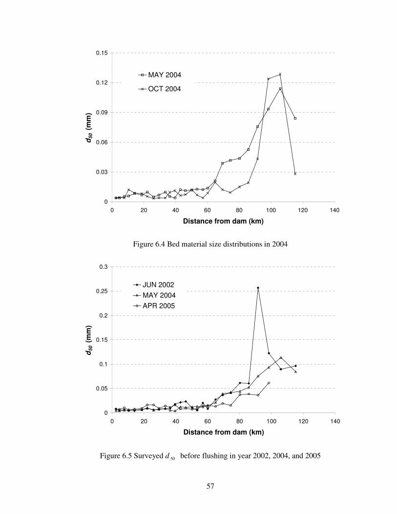
57
0
0.03
0.06
0.09
0.12
0.15
0 20 40 60 80 100 120 140
Distance from dam (km)
d5
0 (
mm
)
MAY 2004
OCT 2004
Figure 6.4 Bed material size distributions in 2004
0
0.05
0.1
0.15
0.2
0.25
0.3
0 20 40 60 80 100 120 140
Distance from dam (km)
d5
0 (
mm
)
JUN 2002
MAY 2004
APR 2005
Figure 6.5 Surveyed d 50 before flushing in year 2002, 2004, and 2005
58
(2) Incoming Sediment Quantity and Size Distribution
GSTARS models require not only the quantity of incoming sediment from the upstream
boundary, but also the size distribution. Daily or monthly incoming sediment data are
needed for GSTARS4 simulation.
The Yang et al. (1996) sediment transport equation, developed for high concentration
sediment laden flow in the Yellow River, was used for this study. To use this method,
information on the percentage of wash load is required. The percentage of wash load
depends on field conditions. It is desirable to have surveyed bed material and suspended
material sediment size distributions to determine the percentage of fine material
transported as wash load.
Because the wash load fraction was not available, it was assumed that sediment size less
than 0.01 mm was the wash load (Yang, 1996 and 2003) of total incoming sediment.
Yang (1996 and 2003) found that even if the initially assumed wash load percentage is
not accurate, the Yang et al. (1996) method can still give fairly good estimation of bed-
material load in the Yellow River with high concentration of wash load. Therefore, bed-
material load computation using the Yang et al. (1996) method is valid for this study.
Daily incoming sediment size distributions were available and monthly averaged values
were used for GSTARS4 modeling because the variation in a month was small.
59
(3) Density of Deposited Sediment
Because dry specific weight or mass of bed materials in the Xiaolangdi Reservoir was not
available, these values were estimated using the method recommended by Yang (1996
and 2003). There are usually four types of reservoir (U.S. Bureau of Reclamation, 1987)
with different densities of deposited sediment. Classification of reservoir operation and
dry specific mass of bed material are shown in Table 6.1 and 6.2, respectively.
The study reach is from Xiaolangdi Dam to Sanmenxia Dam. This study reach has a
length of about 120km long and consists of both reservoir and river regimes. Density of
deposited sediment in the reservoir regime can be classified as operation number 2, while
that in the river regime should be operation number 4, “Riverbed sediments”. The flow
characteristics in the study reach should be divided into reservoir and river regimes. In
the downstream reach, the flow is very slow and deep due to backwater effect. This reach
can be classified as a reservoir regime. In the upper reach, upstream of the backwater, it
is classified as a river reach. Therefore, sediment density in the reservoir reach has to be
operation number 2 and that in river reach should be operation number 4. In other words,
different sets of deposited sediment density must be used for computation. In this study, a
combination operation number 2 for reservoir regime and number 4 for river regime was
used for the simulation. However, simulations with operation number 1 for reservoir and
number 4 for river were conducted for comparison.
As shown in Table 6.2, density variation of clay is significant, whereas for coarser
materials of silt and sand the density is fairly constant regardless of the operation number.
It is assumed that consolidation effect is negligible in this study due to annual flushing

60
operations. Generally speaking, the density of bed sediments may change with respect to
time due to consolidation. For fine materials, such as clay and silt, these effects are
important for the determination of deposited sediment volume in a reservoir.
Consolidation is not considered in this study because a large portion of deposited
sediment is scoured out during drawdown flushing each year. Sediment deposited in the
Xiaolangdi Reservoir does not have enough time to be consolidated because of annual
drawdown flushing.
Table 6.1 Four types of reservoir operation
Operation Reservoir operation
1 Sediment always submerged or nearly submerged
2 Normally moderated to considerable reservoir drawdown
3 Reservoir normally empty
4 Riverbed sediments
Table 6.2 Initial dry specific mass with respect to operation number
Initial dry specific mass (kg/m3)
Operation Clay Silt Sand
1 416 1120 1550
2 561 1140 1550
3 641 1150 1550
4 961 1170 1550

61
6.1.3 Cross Section Geometry Data
Cross section geometry of the Xiaolangdi Reservoir and its tributaries were surveyed six
times, i.e., January 2000, May and October 2003, May and October 2004, and October
2006. Fig. 6.6 shows the surveyed thalweg profiles of the study reach. In the first three
years of operation, from January 2000 to May 2003, deposition occurred significantly and
rapidly in the reservoir reach, from the dam to about 60 km. After the first three years,
deposition also occurs in the reservoir reach but less than occurred in the first three years.
There are 56 sets of cross sectional data with about 2 km spacing between cross sections.
GSTARS4 simulation cannot be conducted using all 56 cross sections because 2 km
spacing does not satisfy the stability criteria of the numerical simulation and the results
are unstable. Determination of spacing is explained in section 6.2.
100
120
140
160
180
200
220
240
260
280
300
0 20 40 60 80 100 120 140
Distance from dam (km)
Th
alw
eg
ele
va
tio
n (
m)
JAN 2000(initial bed) MAY 2003
OCT 2003 MAY 2004
OCT 2004 OCT 2006
Figure 6.6 Measured thalweg elevation

62
6.1.4 Water Temperature Data
Water viscosity, density, and sediment fall velocity are all affected by water temperature.
It is necessary to use accurate water temperature data for the GSTARS4 simulation.
However, there is no water temperature data for the Xiaolangdi Reservoir. Therefore,
water temperature was assumed for each month. Table 6.3 shows assumed water
temperature.
Table 6.3 Water temperature of Xiaolangdi Reservoir (assumed values)
Month Jan Feb Mar Apr May Jun Jul Aug Sep Oct Nov Dec
Temperature (◦C) 5 5 5 8 8 10 10 16 10 8 5 5
6.1.5 Tributary Volume Data
There are more than 40 tributaries flowing into the Xiaolangdi Reservoir. Twelve of them
were considered as major tributaries and the total volume of the small tributaries were
combined into an “imaginary tributary” with the location shown in Fig. 1.2. Twelve
major tributaries plus the imaginary tributary were considered in this study. The
relationship between water surface elevation and volume of tributaries can be computed
by Eq. (4.2). The parameters used in Eq. (4.2) are summarized in Table 6.4.

63
Table 6.4 Water stage and tributary volume relationships
Name of
Tributaries
Location of the Mouth
(m, distance from Xiaolangdi dam) 1v 2v hm
Simengou 600 666.99 2.5337 154.66
Dayuhe 4225 4404.6 2.4357 149.90
Meiyaogou 6350 102.89 2.9786 159.80
Baimahe 10355 187.71 2.7099 169.70
Zhenshuihe 17030 4545.2 2.6260 154.40
Shijinghe 21680 3177.5 2.4643 160.40
Donyanghe 29100 126.94 3.1193 171.40
Xiyanghe 39380 4659.1 2.3461 179.50
Ruicunhe 42410 6043.5 2.1970 178.20
Imaginary Tributary 52000 2286.8 2.9175 182.69
Yunxihe 54570 39380 2.0472 196.10
Boqinghe 56950 6803.6 2.3956 216.10
Banjianhe 61590 4158.2 2.2154 208.40
6.2 Determination of Time Step and Distance between Cross Sections
GSTARS models use a finite difference uncoupled scheme, which means that hydraulic
properties are calculated first. Sediment routes and bed changes are computed after the
hydraulic computation, keeping all the hydraulic parameters fixed during the calculation
(Yang and Simões, 2002). During a time step ∆t, hydraulic properties and channel
boundary changes should be small because the channel boundary is assumed to be fixed
during the hydraulic property calculation.
GSTARS3 model calculates the change of cross sections due to scour or deposition using
Eq. (3.13). From Eq. (3.13), it is clear that the bed elevation change is related to ∆t. When
the bed elevation change during ∆t is small compared to flow depth, the assumption of
rigid boundary is valid for hydraulic property calculation, and the aggradation-
degradation calculation can be performed by the uncoupled scheme (Julien, 2002).

64
In this study, the simulations were carried out from May 2003 to October 2006 when
surveyed cross section geometry data were available for comparison; ∆t = 3 minutes, 6
minutes, and 10 minutes were tested. Fig. 6.7 shows the simulated results using different ∆t
values. In the circled area near the reservoir delta with data of October 2006, the result of
∆t = 3 minutes agrees best with the surveyed data. In other areas, ∆t = 3 minutes and ∆t = 6
minutes give similar results. Because the rate of scour or deposition near the reservoir delta
is important, simulation with ∆t = 3 minutes was used in this study.
100
120
140
160
180
200
220
240
260
280
300
0 20 40 60 80 100 120 140
Distance from dam (km)
Th
alw
eg
ele
va
tio
n (
m)
Initial bed (May 2003)
Surveyed (Oct. 2006)
Simulated (∆t=3min)
Simulated (∆t=6min)
Simulated (∆t=10min)
(∆t = 3 min.)
(∆t = 6 min.)
(∆t = 10 min.)
Figure 6.7 Comparison of longitudinal profiles using different time steps
(∆t = 3, 6, and 10 minutes)

65
Stability criteria for sediment transport and channel adjustment were derived in section
5.1 and 5.2 with the assumptions of a wide rectangular channel with constant width. Time
step and distance between cross sections should satisfy Eq. (5.14) and Eq. (5.25) for
quasi-steady and unsteady simulations, respectively.
For the Xiaolangdi Reservoir sediment and bed change computation,
11
12
≅− Fr
(6.1a)
( )( )
111
122
−≅−−
−β
β
β
Fr (6.1b)
If the Manning’s equation is used, β = 5/3
5.55 << b , b = 5.3 is used (6.1c)
55.03.0 <<η in river regime, 4.0=η is used (6.1d)
V and Cv are the mean flow velocity and sediment transport capacity, respectively. These
values depend on the flow condition, which is a function of time and cross section
location. The bed change in the upstream reach is faster than that in the downstream
reach. Therefore, values for the upstream reach should be used. For this study, V and Cv
values in the upstream reach, at 110 km above Xiaolangdi Dam and about 10 km below
Sanmenxia Dam, were considered.
To satisfy the stability criteria, the following maximum value should be used.
[ ] 0.3≅vVCMAX (m/s) (6.1e)
This maximum value occurred in August 2004.
66
Eq. (5.14) and (5.25) give the stability criteria for the Xiaolangi Reservoir sedimentation
routing in the upstream reach, for steady and unsteady simulations, respectively.
The condition for stable computational results with an explicit scheme can be determined
by substituting Eqs. (6.1a) ~ (6.1e) to Eqs. (5.14) and (5.25).
The condition of the stable solution for a steady simulation is
8.39≥∆
∆
t
x (in m/s) (6.2a)
Similarly, the condition for an unsteady simulation is
5.26≥∆
∆
t
x (in m/s) (6.2b)
For the same ∆t, Eqs. (6.2a) and (6.2b) reveal that steady simulation requires a longer ∆x
than that of unsteady simulation.
With ∆t = 3 minute (180 second), then ∆x ≥ 7200 m and 4800 m for steady and unsteady
simulations, respectively. To satisfy Eq. (6.2a) in river regime, from Sanmenxia dam to
about 55 km above Xiaolangdi dam, ∆x > 7200 m.
VCv values vary with respect to location. The upstream reach has larger values than the
downstream reach, because the downstream reach is in the reservoir regime and the
upstream reach is in the river regime. Therefore,
reservoirriver xx ∆≥∆ (6.3)
where riverx∆ and reservoirx∆ = distance between cross sections for the river and reservoir
reaches, respectively.
Shorter ∆x values were tried for the downstream reservoir reach, and the simulated results
did not show any numerical instability. In this study, ∆t, ∆xriver, and ∆xreservoir are the same

67
for steady and unsteady simulations. Fig. 6.8 (b) shows unstable mean bed material size,
d50, in the upper reach using 56 cross sections in August 2008 when Eq. (6.1e) is used.
Therefore, ∆xriver > 7200 m was selected for this study.
0
0.03
0.06
0.09
0.12
0.15
0 50 100 150Distance from dam (km)
d5
0 (m
m)
Initial (MAY 2003)
Simulated (AUG. 2004)
(a) 24 Cross sections (∆xriver > 7200 m)
0
0.03
0.06
0.09
0.12
0.15
0 50 100 150Distance from dam (km)
d5
0 (m
m)
Initial (MAY 2003)
Simulated (AUG. 2004)
(b) 56 Cross sections (∆xriver < 7200 m)
Figure 6.8 Bed material size profile with steady simulation using 24 and 56 cross sections

68
6.3 Calibration of Coefficients
6.3.1 Roughness Coefficient (Manning’s n)
Manning’s n values vary along the study reach with respect to time. However, it is very
difficult to find a functional relationship between the roughness coefficient and time. It is
assumed that Manning’s n is a function of cross section location and man particle
diameter.
Determination of the variation of the roughness coefficient along the main reservoir is
important for the numerical model. It is reasonable to assume that Manning’s n decreases
in the downstream direction due to the decrease of sediment particle size. Manning’s n
value for each cross section could be determined as a function of d50. Six sets of surveyed
data on bed material size distributions, i.e., June 2002, October 2003, May and October
2004, and April and November 2005, were provided. Bed material sizes surveyed in
those years are similar to each other. The measured results at about 95 km in June 2002
shown in Fig. 6.5 are unusually high. This is because the upstream reach is directly
controlled by discharged sediment from the Sanmenxia reservoir. The sediment size
profile for 2002 was used to determine Manning’s n value.
Fig. 6.9 shows d50 variation along the study reach. The relationship between d50 and
location can be divided into two regimes, i.e., reservoir and river regimes. The
relationship between d50, in mm, and distance from Sanmenxia Dam is
xed
0171.0
50 0051.0 ×= for reservoir regime, below 60 km from the dam (6.4a)
xed
0262.0
50 0061.0 ×= for river reaches, above 60 km from the dam (6.4b)

69
Eqs. (6.4a) and (6.4b) were used initially to determine Manning’s n values for the study
area.
The final Manning’s n values for all cross sections were derived using the following
relationship.
6/1
50dn ∝ , 6/1
50dn ⋅= κ ( 50d in mm) (6.5)
where κ = a coefficient.
Two separate κ values are required for river and reservoir regimes, respectively, as shown
in Fig. 6.9. κ values of 0.063 and 0.022 were used for river and reservoir regimes,
respectively. These relationships are
6/1
50063.0 dn = , in river regime (6.6a)
6/1
50022.0 dn = , in reservoir regime (6.6b)
Fig. 6.10 (a) Manning’s n suddenly increases around 60 km ~ 61 km. Fig. 6.10 (a)
indicates that n value suddenly increases around 60 ~ 61 km without a gradual transition
between 50 ~ 90 km where the reservoir regime gradually changed to the river regime.
The variation of n value along the study reach with a transition between reservoir and
river reaches shown in Fig. 6.10 (b) was used for this study.

70
d 50 = 0.0051e0.0171x
R2 = 0.3452
d 50 = 0.0061e0.0262x
R2 = 0.8228
0
0.02
0.04
0.06
0.08
0.1
0.12
0.14
0 20 40 60 80 100 120 140
Distance from dam (km)
d50 (
mm
)
Reservoir regime
River regime
Figure 6.9 Measured d50 along the main reservoir reach in June 2002
0
0.01
0.02
0.03
0.04
0.05
0 20 40 60 80 100 120 140
Distance from dam (km)
Ma
nn
ing
's n
(a) Manning’s n values using Eqs. (6.6a) and (6.6b)
0
0.01
0.02
0.03
0.04
0.05
0 20 40 60 80 100 120 140
Distance from dam (km)
Ma
nn
ing
's n
(b) Manning’s n values for this study (gradual variation around the transient)
Figure 6.10 Variation of Manning’s n values used for the simulation

71
6.3.2 Recovery Factor
Sediment size is divided into nine groups in this study. Each group has a lower and an
upper limit of diameter and the representative size for each group is the geometric mean
value of the limits, as shown in Table 6.5. In Eq. (4.7), two coefficients are required to
determine the recovery factor α. Combinations of coefficients in Eq. (4.7) were calibrated
by trial-and-error method with steady simulations. The duration of simulations for the
calibration was 3.5 years from May 2003 to October 2006. The calibration process was
carried out by comparing simulated thalweg profiles to measured ones. The goodness-of-
fit of thalweg elevations was evaluated by two statistical parameters, the root-mean-
square (RMS) and the average geometric deviation (AGD). Two parameters are
computed as follows.
(1) RMS
RMS = ( )2/1
1
2/
−∑
=
J
j
mjcj Jzz (6.7)
where zc and zm = computed and measured elevations in meter, respectively; j = index of
data set; and J = total number of data set. The unit of RMS for bed elevation is in meter.
(2) AGD
AGD =
JJ
j
jR
/1
1
∏
=
, cjmj
mjcj
jzz
zzR
/
/=
mjcj
mjcj
zz
zz
<
≥ (6.8)
where Rj = special discrepancy ratio. AGD is a dimensionless parameter.
Computed RMS and AGD for some of combinations of ε and ξ were summarized in
Table 6.6 (a) and (b), respectively. The calibrated values of ε and ξ were 0.17 and 0.3,
for
for

72
respectively, because the combination provides the lowest RMS and AGD for the every
comparison only except October 2004. Each coefficient has the same value for scour and
deposition. The need to consider using different coefficient values for scour and
deposition, suggested by Han and He (1990), was not found for the Xiaolangdi Reservoir
study. This conclusion seems reasonable because the difference between scour and
deposition reflects the change of the bed material size gradation. Recovery factors, which
vary from 0.189 to 0.988, with calibrated coefficients are shown in Table 6.7. Calibration
of two coefficients may be required for other reservoir sedimentation.
Table 6.5 Sediment size group for this study
Group Lower bound (mm) Upper bound (mm) Geometric mean (mm)
1 0.002 0.004 0.00283
2 0.004 0.008 0.00563
3 0.008 0.016 0.0113
4 0.016 0.031 0.0223
5 0.031 0.062 0.0438
6 0.062 0.125 0.0880
7 0.125 0.25 0.1768
8 0.25 0.5 0.3536
9 0.5 1 0.7071
Table 6.6 (a) Calibration of recovery factor, RMS of thalweg elevation
RMS (m)
Time ε ξ OCT.
2003
MAY
2004
OCT.
2004
NOV.
2005
OCT.
2006
Average Remarks
0.5 0.1 5.93 5.39 6.18 5.02 7.32 5.97
0.1 0.1 10.62 7.24 5.70 4.53 7.95 7.21
0.3 0.2 5.77 5.31 5.82 4.78 7.25 5.79
0.1 0.2 9.01 5.04 5.77 4.26 7.42 6.30
0.1 0.3 7.23 4.71 5.87 4.26 6.42 5.70
0.17 0.3 4.99 4.15 6.42 3.83 4.55 4.79 Lowest
0.2 0.3 5.66 5.16 5.42 3.84 5.74 5.16
0.05 0.4 9.60 5.23 5.68 4.19 7.10 6.36
0.1 0.4 6.05 4.63 5.44 3.92 5.45 5.10
0.05 0.5 7.61 4.45 5.80 4.19 6.23 5.66
0.02 0.5 13.19 9.59 8.57 5.87 6.03 8.65
Han and He (1990) 6.92 5.25 5.83 4.13 7.32 5.89

73
Table 6.6 (b) Calibration of recovery factor, AGD of thalweg elevation
AGD
Time ε ξ OCT.
2003
MAY
2004
OCT.
2004
NOV.
2005
OCT.
2006
Average Remarks
0.5 0.1 1.022 1.020 1.026 1.019 1.028 1.022
0.1 0.1 1.029 1.021 1.024 1.018 1.030 1.029
0.3 0.2 1.022 1.020 1.026 1.018 1.029 1.022
0.1 0.2 1.026 1.017 1.024 1.016 1.027 1.026
0.1 0.3 1.024 1.016 1.025 1.016 1.024 1.024
0.17 0.3 1.020 1.016 1.027 1.016 1.018 1.020 Lowest
0.2 0.3 1.022 1.019 1.022 1.014 1.021 1.022
0.05 0.4 1.027 1.017 1.024 1.016 1.026 1.027
0.1 0.4 1.022 1.017 1.022 1.015 1.020 1.022
0.05 0.5 1.023 1.015 1.024 1.016 1.022 1.023
0.02 0.5 1.034 1.024 1.028 1.018 1.021 1.034
Han and He (1990) 6.92 1.024 1.018 1.025 1.016 1.027
Table 6.7 Calibrated recovery factor for both scour and deposition
Size
group
Lower bound
(mm)
Upper bound
(mm)
Geometric
mean (mm) Recovery factor
1 0.002 0.004 Coarse clay 0.989
2 0.004 0.008 Very fine silt 0.803
3 0.008 0.016 Fine silt 0.652
4 0.016 0.031 Medium silt 0.532
5 0.031 0.062 Coarse silt 0.434
6 0.062 0.125 Very fine sand 0.352
7 0.125 0.25 Fine sand 0.286
8 0.25 0.5 Medium sand 0.232
9 0.5 1 Coarse sand 0.189
6.4 Xiaolangdi Reservoir Sedimentation and Flushing Simulation Results
Simulations from May 2003 to October 2006 were carried out to verify the capabilities of
GSTARS4 for quasi-steady and truly unsteady flows. A total of four cases of simulations,
shown in Table 6.8, were compared in this section.

74
All the simulations were carried out using ∆t = 3 minutes and the Yang et al. (1996)
sediment transport equation with the recovery factor of 3.0
17.0
k
kd
=α .
The simulated bed profile, bed material size, volume of sedimentation, and gradation of
flushed sediment were compared with the surveyed values in the following sections.
Table 6.8 Four simulations of Xiaolangdi Reservoir from May 2003 to October 2006
Density of bed sediment
(values shown in Table 6.2) Case of simulation Flow routing
In reservoir regime In river regime
Steady_OP1 Operation No. 1 Operation No. 4
Steady_OP2 Quasi-steady
Operation No. 2 Operation No. 4
Unsteady_OP1 Operation No. 1 Operation No. 4
Unsteady_OP2 Truly unsteady
Operation No. 2 Operation No. 4
6.4.1 Thalweg Profile
Bed profiles were surveyed several times between 2003 and 2006. These surveyed profiles
were compared with those computed by GSTARS4.
RMS and AGD were compared for four simulation cases, as shown in Table 6.9 (a) and (b),
respectively. Simulations using sediment density of operation number 1, Steady_OP1 and
Unsteady_OP1, have lower RMS and AGD than the other. However, simulations cases of
“OP1” were conducted only for the comparison and density of deposited sediment in the
reservoir should be operation number 2, “OP2”. Steady results have lower RMS and AGD
values of thalweg elevations than unsteady ones. The prediction of channel geometric
changes by GSTARS4 steady and unsteady simulations should be evaluated by comparing
not only thalweg elevation changes but also by cross section changes. Statistical

75
evaluations on the predicted cross section changes by using steady and unsteady
simulations are included in section 6.4.2.
Fig. 6.11 shows comparisons between measured and simulated thalweg elevations. In Fig.
6.11 (a) ~ (d), the surveyed thalweg values are slightly lower than the simulated results
near Xiaolangdi Dam because the effect of the sediment flushing gates was not
considered. It was difficult to consider the effect of the low level flushing gates because
the data related to the operation of these gates were not available, therefore the effects of
low level outlets were not included in this study.
A comparison between operation number 1 and 2 reveals that the simulation results with
operation number 2 generally have higher thalweg elevation than those with operation
number 1, as shown in Figs. 6.11 (a) ~ (d). Because the sediment density of operation
number 1 is lower than that of operation number 2, the simulated results with operation
number 1 have lower bed elevation.
Table 6.9 (a) RMS of thalweg elevation
RMS (m)
Time Case of simulation OCT.
2003
MAY
2004
OCT.
2004
NOV.
2005
OCT.
2006
Average
Steady_OP1 4.95 4.08 6.46 3.87 4.13 4.70
Steady_OP2 4.99 4.15 6.42 3.83 4.55 4.79
Unsteady_OP1 5.93 5.48 6.24 3.57 5.04 5.25
Unsteady_OP2 6.28 5.90 6.42 4.24 6.04 5.78
Table 6.9 (b) AGD of thalweg elevation
AGD
Time Simulation OCT.
2003
MAY
2004
OCT.
2004
NOV.
2005
OCT.
2006
Average
Steady_OP1 1.020 1.016 1.027 1.016 1.015 1.019
Steady_OP2 1.020 1.016 1.027 1.016 1.018 1.020
Unsteady_OP1 1.020 1.017 1.024 1.013 1.017 1.018
Unsteady_OP2 1.022 1.020 1.025 1.018 1.022 1.021

76
160
180
200
220
240
260
280
300
0 20 40 60 80 100 120 140
Distance from the dam (km)
Th
alw
eg
ele
va
tio
n (
m)
Initial bed (MAY 2003)Survey (OCT 2003)Steady_OP1 (OCT 2003)Steady_OP2 (OCT 2003)Unsteady_OP1 (OCT 2003)Unsteady_OP2 (OCT 2003)
(a) October 2003
160
180
200
220
240
260
280
300
0 20 40 60 80 100 120 140
Distance from the dam (km)
Th
alw
eg
ele
va
tio
n (
m)
Initial bed (MAY 2003)
Survey (OCT 2004)
Steady_OP1 (OCT 2004)
Steady_OP2 (OCT 2004)
Unsteady_OP1 (OCT 2004)
Unsteady_OP2 (OCT 2004)
(b) October 2004
Figure 6.11 Comparison of surveyed and simulated thalweg elevations

77
160
180
200
220
240
260
280
300
0 20 40 60 80 100 120 140
Distance from the dam (km)
Th
alw
eg
ele
va
tio
n (
m)
Initial bed (MAY 2003)Surveyed (NOV 2005)Steady_OP1 (NOV 2005)Steady_OP2 (NOV 2005)Unsteady_OP1 (NOV 2005)Unsteady_OP2 (NOV 2005)
(c) November 2005
160
180
200
220
240
260
280
300
0 20 40 60 80 100 120 140
Distance from the dam (km)
Th
alw
eg
ele
va
tio
n (
m)
Initial bed (MAY 2003)Surveyed (OCT 2006)Steady_OP1 (OCT 2006)Steady_OP2 (OCT 2006)Unsteady_OP1 (OCT 2006)Unsteady_OP2 (OCT 2006)
(d) October 2006
Figure 6.11 Continued

78
6.4.2 Cross Sectional Changes
Figs. 6.12 ~ 6.15 show comparisons of simulated and measured cross sections.
Simulations results of steady flow reservoir operation type 1 (Steady_OP1) and unsteady
flow operation type 1 (Unstead_OP1) are shown in Appendix A.
Results shown in Figs. 6.12 ~ 6.15 indicate that the steady and unsteady flow simulation
results are generally in agreement with the measured results. However, the steady
simulation predicts a narrowing of the river regime after October 2004. The unsteady
effect in the river regime was not significant in 2003. The rate of water surface drop in
2003 was less than that of 2004, 2005, and 2006, as shown in Fig. 6.1. Water discharge
from the upstream boundary in 2003 was the smallest from 2003 to 2006. Steady
simulation results of October 2003 and May 2004 do not have a narrow of the cross
section because the unsteady effect is small in 2003. However, the unsteady effect should
be considered after May 2004 and the steady simulation predicts narrowing of the
channel. Fig. 6.13 (a), (b), and (c) show the formation of a narrow channel for the steady
simulation while the unsteady flow simulations predict a wide channel. A comparison of
Figs. 6.12 (a) ~ (c) and Figs. 6.13 (a) ~ (c) shows scour pattern at the upper reach in
October 2003 and October 2004. The unsteady flow simulation predicts more scour than
the steady flow simulation results. Water discharge from the upstream boundary increases
suddenly, as shown in Fig. 6.1, and variation of water stage and discharge follows loop-
rating curve. The rising limb has more unit stream power, VS, than the falling limb
because the former has higher friction slope and faster flow velocity. Therefore, both
limbs have various sediment transport capacities. Unsteady simulation computes
sediment transport capacities for both limbs. Sum of sediment transport capacities of

79
rising and falling limb from unsteady simulation is not the same as that computed from
steady simulation, because the sediment transport capacity is not liner to the unit stream
power, as shown in Eq. (3.15). The steady flow simulations show a narrowing of the river
regime after October 2004. Simulation results of the lower reach are better than those of
the upper reach. This is because upstream cross sections are directly influenced by the
discharged water and sediment from the Sanmenxia Reservoir. Scour and deposition in
the lower reaches, about 10 ~ 60 km above the Xiaolangdi dam, is less dependent on the
upstream condition. Figs. 6.13 (a), (b), and (c) show the scour due to drawdown flushing.
The unsteady flow simulations show similar results. The scour in the upper reach was
mainly caused by water discharged from the upstream Sanmenxia Reservoir. The trend
also can be found in Fig. 6.1. Because water and sediment discharge from Sanmenxia
Dam varies rapidly, the unsteady effect should be considered for this study area. The
predicted channel cross section changes in the reservoir regime, from Xiaolangdi Dam to
50 ~ 60 km above it, are close to measurements because the effect of water flow released
from the upstream dam attenuates as it goes downstream and the unsteady effects
decrease.
To evaluate the performance of both steady and unsteady simulation, RMS and AGD
were computed for each cross section by using Eqs, (6.7) and (6.8), respectively. Figs.
6.16 and 6.17 show comparison of statistical parameters of steady and unsteady
simulations, respectively. Steady simulation results of the lower reach are better than
those of the upper reach because the unsteady effect due to sudden release of water from
the upstream boundary diminished in the downstream direction, as shown in Fig. 6.16.
Fig. 6.16 (a) indicates that RMS values in October 2003 and May 2004 are all lower than

80
8 m along the study area. However, RMS values after October 2004, increased
significantly in the upper reach, because the steady simulation predicted narrower
channel. Similarly trend was also found for AGD values, as shown in Fig. 6.16 (b). Fig.
6.17 (a) and (b) show RMS and AGD of unsteady simulation and there is no increase of
both parameters in the upper reach after October 2004.
Averaged values of RMS and AGD are summarized in Table 6.10 (a) and (b),
respectively. As described above, RMS and AGD values were computed for every cross
section at every time of comparison. Values shown at each line is the averaged RMS and
AGD of all the cross sections. For example, values on line (1) of Table 6.10 (a) are the
averages of RMS along the study area in October 2003. Before May 2004, steady
simulation has lower RMS than unsteady by 0.2 ~ 0.4 m. However, steady simulation has
higher RMS by 1.3 ~ 2.5 m after October 2004. Unsteady simulation has lower RMS.
The same trend is found with AGD values, as summarized in Fig. 6.10 (b). Unsteady
simulation has better prediction of cross section geometry changes, especially for the
upper reach due to sudden inflow of water sediment from the upstream Sanmenxia
reservoir, because unsteady flow simulation can compute sediment transport capacities of
the rising and fall stages of the sudden inflow.

81
230
250
270
290
310
0 200 400 600 800Lateral (m)
Ele
vati
on
(m
)
Initial bed (MAY 2003)
Surveyed (OCT. 2003)
Steady_OP2 (OCT. 2003)
Unsteady_OP2 (OCT. 2003)
210
230
250
270
0 200 400 600Lateral (m)
Ele
vati
on
(m
)
(a) 101.6 km above Xiaolangdi dam (b) 80.2 km
200
220
240
260
0 200 400 600Lateral (m)
Ele
vati
on
(m
)
200
220
240
260
500 1000 1500 2000 2500Lateral (m)
Ele
vati
on
(m
)
(c) 72.1km (d) 57.0km
200
220
240
260
0 500 1000Lateral (m)
Ele
va
tio
n (
m)
180
200
220
240
0 200 400 600Lateral (m)
Ele
vati
on
(m
)
(e) 43.0 km (f) 27.2 km
170
190
210
230
0 500 1000 1500 2000Lateral (m)
Ele
vati
on
(m
)
170
190
210
230
0 300 600 900 1200Lateral (m)
Ele
vati
on
(m
)
(g) 18.7 km (h) 11.4 km
Figure 6.12 Comparisons between measured and GSTARS4 simulation results, October
2003

82
230
250
270
290
310
0 200 400 600 800Lateral (m)
Ele
vati
on
(m
)
Initial bed (MAY 2003)Surveyed (OCT. 2004)Steady_OP2 (OCT. 2004)Unsteady_OP2 (OCT. 2004)
210
230
250
270
0 200 400 600Lateral (m)
Ele
vati
on
(m
)
(a) 101.6 km above Xiaolangdi dam (b) 80.2 km
200
220
240
260
0 200 400 600Lateral (m)
Ele
va
tio
n (
m)
200
220
240
260
500 1000 1500 2000 2500Lateral (m)
Ele
vati
on
(m
)
(c) 72.1km (d) 57.0km
200
220
240
260
0 500 1000Lateral (m)
Ele
va
tio
n (
m)
180
200
220
240
0 200 400 600Lateral (m)
Ele
vati
on
(m
)
(e) 43.0 km (f) 27.2 km
170
190
210
230
0 500 1000 1500 2000Lateral (m)
Ele
vati
on
(m
)
170
190
210
230
0 300 600 900 1200Lateral (m)
Ele
vati
on
(m
)
(g) 18.7 km (h) 11.4 km
Figure 6.13 Comparisons between measured and GSTARS4 simulation results, October
2004

83
230
250
270
290
310
0 200 400 600 800Lateral (m)
Ele
vati
on
(m
)
Initial bed (MAY 2003)Surveyed (NOV. 2005)Steady_OP2 (NOV. 2005)Unsteady_OP2 (NOV. 2005)
210
230
250
270
0 200 400 600Lateral (m)
Ele
vati
on
(m
)
(a) 101.6 km above Xiaolangdi dam (b) 80.2 km
200
220
240
260
0 200 400 600Lateral (m)
Ele
vati
on
(m
)
200
220
240
260
500 1000 1500 2000 2500Lateral (m)
Ele
vati
on
(m
)
(c) 72.1km (d) 57.0km
200
220
240
260
0 500 1000Lateral (m)
Ele
va
tio
n (
m)
180
200
220
240
0 200 400 600Lateral (m)
Ele
vati
on
(m
)
(e) 43.0 km (f) 27.2 km
170
190
210
230
0 500 1000 1500 2000Lateral (m)
Ele
va
tion
(m
)
170
190
210
230
0 300 600 900 1200Lateral (m)
Ele
vati
on
(m
)
(g) 18.7 km (h) 11.4 km
Figure 6.14 Comparisons between measured and GSTARS4 simulation results,
November 2005

84
230
250
270
290
310
0 200 400 600 800Lateral (m)
Ele
vati
on
(m
)
Initial bed (MAY 2003)Surveyed (OCT. 2006)Steady_OP2 (OCT. 2006)Unsteady_OP2 (OCT. 2006)
210
230
250
270
0 200 400 600Lateral (m)
Ele
vati
on
(m
)
(a) 101.6 km above Xiaolangdi dam (b) 80.2 km
200
220
240
260
0 200 400 600Lateral (m)
Ele
vati
on
(m
)
200
220
240
260
500 1000 1500 2000 2500Lateral (m)
Ele
vati
on
(m
)
(c) 72.1km (d) 57.0km
200
220
240
260
0 500 1000Lateral (m)
Ele
va
tio
n (
m)
180
200
220
240
0 200 400 600Lateral (m)
Ele
vati
on
(m
)
(e) 43.0 km (f) 27.2 km
170
190
210
230
0 500 1000 1500 2000Lateral (m)
Ele
vati
on
(m
)
170
190
210
230
0 300 600 900 1200Lateral (m)
Ele
va
tio
n (
m)
(g) 18.7 km (h) 11.4 km
Figure 6.15 Comparisons between measured and GSTARS4 simulation results, October
2006
85
0
5
10
15
20
25
0 20 40 60 80 100 120Distance from dam (km)
RM
S (
m)
OCT. 2003MAY 2004OCT. 2004NOV. 2005OCT. 2006
1.00
1.02
1.04
1.06
1.08
1.10
0 20 40 60 80 100 120Distance from dam (km)
AG
D
OCT. 2003MAY 2004OCT. 2004NOV. 2005OCT. 2006
(a) RMS (b) AGD
Figure 6.16 Comparison of goodness-of-fit between Steady_OP2 and measured results
0
5
10
15
20
25
0 20 40 60 80 100 120Distance from dam (km)
RM
S (
m)
OCT. 2003MAY 2004OCT. 2004NOV. 2005OCT. 2006
1.00
1.02
1.04
1.06
1.08
1.10
0 20 40 60 80 100 120Distance from dam (km)
AG
D
OCT. 2003MAY 2004OCT. 2004NOV. 2005OCT. 2006
(a) RMS (b) AGD
Figure 6.17 Comparison of goodness-of-fit between Unsteady_OP2 and measured results
Table 6.10 (a) Averaged RMS of cross section data
RMS (m)
Time Case of simulation
OCT.
2003 (1)
MAY
2004
(2)
OCT.
2004
(3)
NOV.
2005
(4)
OCT.
2006
(5)
Overall
(average of
1~5)
Steady_OP2 3.56 3.23 6.45 6.60 7.68 5.50
Unsteady_OP2 3.76 3.63 5.14 4.38 5.10 4.40
Table 6.10 (b) Averaged AGD of cross section data
AGD
Time Case of simulation
OCT.
2003 (1)
MAY
2004
(2)
OCT.
2004
(3)
NOV.
2005
(4)
OCT.
2006
(5)
Overall
(average of
1~5)
Steady_OP2 1.014 1.013 1.026 1.027 1.031 1.022
Unsteady_OP2 1.015 1.014 1.021 1.018 1.021 1.018
86
6.4.3 Bed Material Size
Fig. 6.18 shows comparisons between simulated and measured bed material sizes. The
measured and simulated results of sediment size distributions generally decrease in the
downstream direction. For the upper reach, the measured bed material size was mainly
determined by the sediment release from the upstream Sanmenxia Reservoir. It takes time
and distance for the sediment released from the Sanmenxia Reservoir to be fully mixed
with the sediments in the Xiaolangdi Reservoir. This may explain why there are some
discrepancies between the simulated results from GSTARS4 and the measured bed
material size in the upper part of the study area, as shown in Fig. 6.18 (c) and 6.18 (e).
The Xiaolangdi Reservoir delta was formed at about 60 km to 80 km, where bed material
size varies significantly, as shown in Figs 6.18 (b) ~ (e). At the toe of the delta or at about
60 km above the dam, sediment transport and mixing are active. The predicted bed
material sizes with steady and unsteady simulations were evaluated by using RMS and
AGD. Similar to Eq. (6.7) and (6.8), these parameters can be computed from the
following equations.
(1) RMS
RMS = ( )2/1
1
2
,50,50 /
−∑
=
J
j
mjcj Jdd (6.9)
where d50,c and d50,m = computed and measured mean bed material size in mm,
respectively. The unit of RMS for bed material size is in mm.
(2) AGD
AGD =
JJ
j
jR
/1
1
∏
=
, cjmj
mjcj
jdd
ddR
,50,50
,50,50
/
/=
mjcj
mjcj
dd
dd
,50,50
,50,50
<
≥ (6.10)
for
for

87
AGD for mean bed material size is a dimensionless parameter.
Comparison of RMS and AGD are summarized in Table 6.11 (a) and (b). Unsteady
simulation has slightly lower average values of RMS and AGD than those for steady
simulation. Typically, bed material is very fine and the size does not vary significantly in
the reservoir regime regardless of the location. There is an abrupt change of bed material
size near the reservoir delta and d50 in the river regime is much coarser than in the
reservoir. Measured bed material size distribution in the study area has the same trend as
described in section 6.1.2. Computed d50, for steady and unsteady simulations, agrees
with typical bed material size profile. Measured d50 profiles have some variations or
oscillations even in the reservoir reach, as shown in Fig. 6.18 (b) ~ (e) and there is an
abrupt change of measured d50, around 100 km in Fig. 6.18 (c). It is possible that these
uncommon variations of measured d50 profile were due to the difficulty of bed material
measurements. These results indicate that GSTARS4 can be used to predict the variation
of bed material size distribution along the study area for a combination of both river and
reservoir regimes with RMS of 0.0151 ~ 0.0155 mm and AGD of 1.55 ~ 1.80 for the
Xiaolangdi Reservoir.
Table 6.11 (a) RMS of mean bed material size
RMS (mm)
Time Case of simulation OCT.
2003
MAY
2004
OCT.
2004
APR.
2005
NOV.
2005
Average
Steady_OP2 0.0089 0.0148 0.0204 0.0104 0.0232 0.0155
Unsteady_OP2 0.0068 0.0173 0.0225 0.0069 0.0220 0.0151
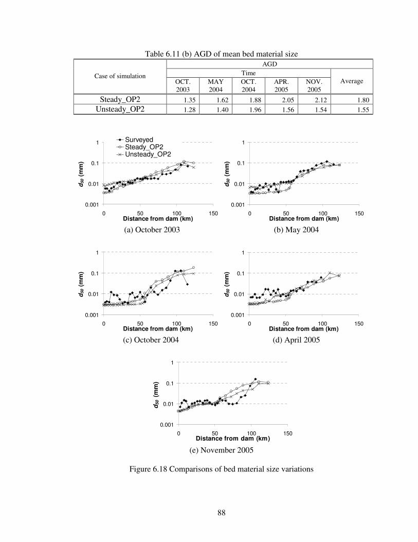
88
Table 6.11 (b) AGD of mean bed material size
AGD
Time Case of simulation OCT.
2003
MAY
2004
OCT.
2004
APR.
2005
NOV.
2005
Average
Steady_OP2 1.35 1.62 1.88 2.05 2.12 1.80
Unsteady_OP2 1.28 1.40 1.96 1.56 1.54 1.55
0.001
0.01
0.1
1
0 50 100 150Distance from dam (km)
d50 (m
m)
SurveyedSteady_OP2Unsteady_OP2
0.001
0.01
0.1
1
0 50 100 150Distance from dam (km)
d50 (m
m)
(a) October 2003 (b) May 2004
0.001
0.01
0.1
1
0 50 100 150Distance from dam (km)
d50 (m
m)
0.001
0.01
0.1
1
0 50 100 150Distance from dam (km)
d50 (m
m)
(c) October 2004 (d) April 2005
0.001
0.01
0.1
1
0 50 100 150Distance from dam (km)
d50 (m
m)
(e) November 2005
Figure 6.18 Comparisons of bed material size variations

89
6.4.4 Yearly Reservoir Sedimentation
The total amount of sedimentation in the Xiaolangdi Reservoir was computed with the
following two methods. The first method compared sediment inflow and outflow.
Sediment inflow into the Xiaolangdi Reservoir was computed by the product of water
inflow and sediment concentration from the upstream Sanmenxia Reservoir. The amount
of sediment flushed out of the Xiaolangdi Reservoir can also be computed as the product
of outflow discharge and sediment concentration. The second method compares the
surveyed reservoir volumes before and after each flushing. The reservoir volume was
surveyed more than twice a year. These surveys were made at the beginning and end of
each flushing. Therefore, the difference between the two sets of surveyed reservoir
volumes give the total amount of sediment flushed out.
Table 6.12 and Fig. 6.19 show comparisons of sedimentation volume using three
different methods. “Measured (in-out)” is based on the product of measured discharge
and concentration at the upstream and downstream boundaries, i.e., Sanmenxia Dam and
Xiaolangdi Dam. “Steady_OP2 (in-out)” and “Unsteady_OP2 (in-out) is based on the
simulated discharge and concentration at the downstream boundary, Xiaolangdi Dam,
using steady and unsteady flow simulations. “Measured reservoir change” is based on a
comparison between the measured reservoir volume before and after flushing.
The results in Table 6.12 and Fig. 6.19 indicate that the simulated volume of
sedimentation using GSTARS4 agrees reasonably well with measured results. The total
volume of sedimentation in the Xiaolangdi Reservoir from May 2003 to October 2006 is

90
about 12×108 m
3. Both steady and unsteady simulations predicted the volumes of
sedimentation are in the same order of magnitude. With the exception of the first year
when the flow regime changed drastically from a river to a reservoir, the unsteady flow
simulation agrees slightly better with the measured data than the steady flow simulation.
Steady simulation slightly under estimates the total volume of sedimentation from 2004
because, the unsteady effect should be considered from 2004, as mentioned in section
6.4.2. Volume of sedimentation was measured for four years. Four measurement results
were used to computed RMS and AGD for both steady and unsteady simulations.
(1) RMS
RMS = ( )2/1
4
1
2
,, 4/
−∑
=j
mjRcjR VV (6.11)
where VR,c and VR,m = computed and measured volume of sedimentation in m3,
respectively. The unit of RMS for the volume of sedimentation is in m3 in this study.
(2) AGD
AGD =
4/14
1
∏
=jjR ,
cjRmjR
mjRcjR
jVV
VVR
,,
,,
/
/=
mjRcjR
mjRcjR
VV
VV
,,
,,
<
≥ (6.12)
The goodness-of-fit evaluation between measured and simulated volume of
sedimentation are summarized in Table 6.13. The ratio between RMS and total volume of
sedimentation was computed as
The ratio between RMS and measured total volume of sedimentation in the Reservoir,
12.2×10⁸ m
3, is less than 5% for both steady and unsteady simulations. Because steady
(6.13) RMS Ratio =
Surveyed total volume of sedimentation (=12.2×10⁸ m
3)
for
for

91
simulation has lower RMS but higher AGD, both steady and unsteady simulations are
good for predicting volume of sedimentation.
Although the simulated volume of sedimentation using GSTARS4 are reasonably
accurate, more studies and field observations should be made before the model can be
applied for long-term prediction with confidence under different reservoir operation plans.
Table 6.12 Comparison of measured and simulated sedimentation volume
Sedimentation Volume (×108 m
3)
Year Measured (in-out)
Measured reservoir
volume change Steady_OP2 (in-out) Unsteady_OP2 (in-out)
2003 6.1 4.80 6.3 7.3
2004 1.0 0.55 0.5 1.3
2005 3.3 3.35 2.6 3.4
2006 1.8 3.43 1.1 1.7
Total 12.2 12.1 10.5 13.6
0
1
2
3
4
5
6
7
8
2003 2004 2005 2006
Year
Sed
imen
tati
on
in
a y
ear
(10
8m
3)
Measured (in-out)
Measured reservoir volume change
Steady_OP2 (in-out)
Unsteady_OP2 (in-out)
Figure 6.19 Measured and simulated sedimentation volumes
Table 6.13 Comparison of measured and simulated sedimentation volume
Simulations case RMS Ratio
(RMS/measured sedimentation) AGD
Steady_OP2 5.69×10⁷ m
3 4.67 % 1.42
Unsteady_OP2 6.08×10⁷ m
3 4.98 % 1.16

92
6.4.5 Gradation of Flushed Sediment
Gradation of flushed sediment is important for the study of flushing impacts downstream.
Figs. 6.20 (a) ~ (d) show gradations of incoming sediment from the upstream reservoir
and flushed sediment out of the Xiaolangdi Reservoir. “Measured in” stands for sediment
input from the upstream boundary and is used as the upstream boundary condition.
“Measured out” is based on the measurement of sediment concentration at Xiaolangdi
Dam. “Steady_OP2 out” and “Unsteady_OP2 out” are based on the simulated results
with operation type 2 with steady and unsteady schemes, respectively.
The sediment input from the upstream reservoir is coarser than that flushed out of the
Xiaolangdi Reservoir. One of the objectives of the Xiaolangdi Reservoir operation is to
regulate sedimentation volume and sediment size distribution. It is desirable to flush fine
sediment rather than coarse materials so flushed sediments can be transported to the sea.
Steady and unsteady simulations do not show any significant difference in the gradation
of flushed sediment. Simulated gradation of flushed sediment both with steady and
unsteady is coarser than the measured data, especially in years 2004 and 2005. The
gradation of flushed sediment is affected by the shape and location of the outlet. In the
Xiaolangdi Reservoir, deposited sediment was flushed through a low level outlet.
However, the low level outlet was not considered, because required field data were not
available. This study focuses on the general trend along the 120 km reach of study during
3.5 years of operation with a 1D model. Simulation of sediment scour and transport near
the low level outlet may require a 2D or 3D model.

93
0
50
100
0.001 0.01 0.1 1Sediment size (mm)
% f
iner
by w
eig
ht
Measured in
Measured out
Steady_OP2 out
Unsteady_OP2 out
0
50
100
0.001 0.01 0.1 1Sediment size (mm)
% f
ine
r b
y w
eig
ht
(a) 2003 (b) 2004
0
50
100
0.001 0.01 0.1 1Sediment size (mm)
% f
iner
by w
eig
ht
0
50
100
0.001 0.01 0.1 1Sediment size (mm)
% f
iner
by w
eig
ht
(c) 2005 (d) 2006
Figure 6.20 Comparisons of incoming and flushed sediment gradation
94
CHAPTER 7. SUMMARY
7.1 Summary and Conclusions
The GSTARS4 model uses an uncoupled scheme to simulate flow and channel
adjustments. GSTARS4 is based mainly on GSTARS3. GSTARS3 can be applied to most
reservoir sedimentation studies. However, flow and sediment transport mechanisms in the
Xiaolangdi Reservoir are very complicated and some of the assumptions made in the
GSTARS3 model may not be valid to fully simulate sedimentation and drawdown
flushing processes of the Xiaolangdi Reservoir. Development of the GSTARS4 model
can be divided into two categories. One is the addition of unsteady flow routing and the
other one is the revision of sediment routing. GSTARS3 can simulate the flow with
steady or quasi-steady schemes. The more advanced unsteady flow scheme adopted from
the SRH-1D model was modified and further improved and included in the GSTARS4
model for fully unsteady flow simulations.
Due to the high sediment concentration in the study reach, time step ∆t and distance
between cross sections ∆x should be determined carefully to assure stable computational
results. If the rate of change of the channel bed is not small enough compared to the water
depth within a time step of computation, it is possible that the computed results may not
be stable. Stability criteria for GSTARS steady and unsteady simulations were derived in
chapter 5 and applied to determine ∆t and ∆x for the Xiaolangdi Reservoir simulation.

95
The study reach is about 120 km long from the downstream boundary, Xiaolangdi Dam,
to the upstream boundary, Sanmenxia Dam. Incoming water and sediment discharges
from the upstream Sanmenxia Reservoir were used as the upstream boundary conditions
in the numerical simulation. Sedimentation process and water flow in the Xiaolangdi
Reservoir are directly affected by water and sediment released from the Sanmenxia
Reservoir. In the upstream reach, just downstream of the Sanmenxia Reservoir, the
channel flow is in the river regime. In the downstream reach, where back water effects
apply, it is in the reservoir regime. Complexity of the simulation arises from the study
area consisting of two regimes, a river and reservoir regime. One major difference
between the two regimes is the density of sediment deposited on the bed. GSTARS4 can
use various densities of deposited sediment in the study area. Site-specific coefficients,
such as Manning’s n and recovery factor were calibrated and determined for the
Xiaolangdi Reservoir.
GSTARS4 was applied to simulate and predict the Xiaolangdi Reservoir variations of
longitudinal profile, cross section, bed material size, and the amount of sedimentation
between May 2003 ~ October 2006. The goodness-of-fit of both steady and unsteady
simulations were evaluated by computing two statistical parameters, RMS and AGD.
Application of the GSTARS4 model to simulate the Xiaolangdi Reservoir sedimentation
and flushing processes produced the following results:

96
1) The simulated longitudinal bed profiles along the study reach, for steady and
unsteady simulations, are generally in good agreement with surveyed profiles,
RMS (4.79 m for steady and 5.78 for unsteady) and AGD (1.020 for steam and
1.021 for unsteady). Especially in the lower reach of study area, computed
profiles are in good agreement with the measured ones.
2) Evaluation of overall goodness-of-fit of cross section geometry indicated that the
unsteady simulation predicted the cross section geometry closer than the steady
simulation for entire 120 km of study area. In the reservoir regime, steady and
unsteady routing predicted almost the same cross section and the predictions are
in good agreement with the measured channel geometry. Both steady and
unsteady simulations have RMS (less than 10 m) and AGD (less than 1.04) in the
reservoir regime. However, unsteady routing predicts more reasonable channel
cross sectional shape than the steady flow simulation in the upstream reach the
river regime. In the upstream reaches, the steady simulation has increased RMS
(from about 5 to 22 m) and AGD (from 1.02 to 1.08) after October 2004, 1.5 year
of routing. The unsteady effects in the upper reach are more significant than in the
lower reach. The release of sediments and water from the upstream Sanmenxia
Reservoir can have a significant influence on the cross section profile and bed
material size distribution in the upper study reach near the upstream Sanmenxia
dam.
3) Simulated bed material size using GSTARS4 steady and unsteady simulations
indicates that predicted bed material follows typical reservoir sedimentation
pattern with finer material in the reservoir and coarser material above the

97
reservoir delta. Unsteady simulation has slightly better result of prediction of d50
than steady simulation, because the former has RMS of 0.0151 mm and AGD of
1.55, while 0.0155 mm and 1.80 for the latter.
4) The ratio between RMS and surveyed total volume of sedimentation is less than
5 % for steady and unsteady simulations.
5) The simulated and measured gradations of flushed sediment are encouraging
because the Xiaolangdi Reservoir can store coarser materials and flush finer
sediments to the downstream Yellow River, reducing the possibility of
downstream deposition.
6) The simulated results using GSTARS4 are in general agreement with measured
results between 2003 and 2006. However, this does not necessarily mean that the
model can be used with confidence for long term simulation of 10, 20, or 30 years
without further verifications. The erosion and sedimentation processes of the
Xiaolangdi Reservoir are complex, and require long term observations of the
reservoir’s operations and their impacts on reservoir sedimentation.
7.2 Contributions
The studies in this dissertation have advanced the technology of numerical modeling of
reservoir sedimentation and flushing in the following areas:
1) GSTARS4 was developed by modifying GSTARS3 and SRH-1D to simulate
steady and unsteady flow sedimentation and flushing processes in reservoirs.
2) Stability criteria for GSTARS4 modeling of sediment transport and channel
geometric changes was derived mathematically.

98
3) The procedure for the numerical simulation of reservoir sediment erosion,
transport, and deposition was developed using the Xiaolangdi Reservoir field data.
Data, required for boundary condition and calibration of coefficients, such as
Manning’s n and recovery factor, for reservoir sedimentation and flushing
simulation, were determined.
7.3 Recommendations for Future Studies
This study focused on the general trend of scour and deposition along a 120 km reach of
the Xiaolangdi Reservoir in 3.5 years using the 1D model GSTARS4, developed for one
dimensional long term and long reach simulation.2D or 3D models should be considered
to simulate sediment scour and transport near the low level outlet.
It is desirable to have a long term simulation with a master plan of reservoir operation.
Long term observation of the Xiaolangdi Reservoir operation is important to understand
the long term reservoir sedimentation process. Long term simulation in the Xiaolangdi
Reservoir verified with field observation with different operational plans may be a good
case study for the reservoir sedimentation model.
Optimization of flushing efficiency may be valuable for future implementation of
drawdown flushing. Flushing efficiency may be improved by increasing the flow rate or
duration of flushing. However, the more water used for flushing, the less water resources
would be left. Therefore, it is better to have an optimized flushing efficiency by carefully
scheduling the flow rate and the duration of flushing.

99
REFERENCES
Ackers, P., and White, W.R. (1973). "Sediment transport: new approach and analysis,"
Journal of the Hydraulic Division, ASCE, Vol. 99, No. HY11, pp. 2041-2060.
Armanini, A., and Di Sivio, G. (1988) “A one-dimensional model for the transport of a
sediment mixture in non-equilibrium condition.” Journal of Hydraulic Research,
Vol.26, No.3, pp. 275-292.
Ashida, K., and Michiue, M. (1970). “Study on suspended sediment (1),” Annals DPRI,
No. 13B, pp. 233-242. (In Japanese.)
Atkinson, E. (1996). Feasibility of flushing sediment from reservoirs, Report OD 137,
HR Wallingford, UK.
Chang, H. H., (1988). Fluvial Processes in River Engineering, John Wiley and Sons,
New York.
Chang, H. H., Harrison, L. L., Lee, W., and Tu, S., (1996). “Numerical modeling for
sediment-pass-though reservoirs,” Journal of Hydraulic Engineering, ASCE, Vol.
122, No. 7, pp. 381-388.

100
Chen, D., Acharya, K., and Stone, M. (2010) “Sensitivity Analysis of Nonequilibrium
Adaptation Parameters for Modeling Mining-Pit Migration.” Journal of Hydraulic
Engineering, ASCE, Vol.136, No.10, pp.806-811.
De Vries, M. (1971). Solving River Problems by Hydraulic and Mathematical Models,
Delft Hydraulic Laboratory, Delft, The Netherlands.
DuBoys, M.P. (1879). “Le Rhône et les rivières à lit affouillable,” Annals de Ponts et
Chaussée, Vol. 18, No. 5, pp. 141-195 (In French).
Engelund, F., and Hansen, E. (1972). A monograph on sediment transport in alluvial
streams, Teknish Forlag, Technical Press, Copenhagen, Denmark.
Fan, J. (1986). “Turbid density currents in reservoirs,” Water Int., Vol. 11, No. 3, pp.
107-116.
Fan, J., and Morris, G. L. (1992a). “Reservoir Sedimentation. I: Delta and Density
Current Deposits.” Journal of Hydraulic Engineering, ASCE, Vol. 118, No. 3, pp.
354-369.
Fan, J., and Morris, G. L. (1992b). “Reservoir Sedimentation. II: Reservoir Desiltation
and Long-Term Storage Capacity.” Journal of Hydraulic Engineering, ASCE, Vol.
118, No. 3, pp. 370-383.

101
Han, Q. (1980). “A Study on the Nonequilibrium Transportation of Suspended Load,”
Proceedings of the International Symposium on River Sedimentation, Beijing,
China, pp. 793-802. (In Chinese.).
Han, Q. (2003). Reservoir sedimentation, Science Publication, Beijing (in Chinese).
Han, Q. (2006). “Diffusion Equation Boundary Condition and Recovery Coefficient,”
Journal of Changsha University of Science and Technology, Vol. 3, No. 3, pp. 7-19.
(in Chinese).
Han, Q., and He, M. (1990). “A Mathematical Model for Reservoir Sedimentation and
Fluvial Processes,” International Journal of Sediment Research, vol. 5, no. 2,
IRTCES, pp. 43-84.
Henderson, F.M. (1966). Open channel flow, MacMillan Book Company, New York, NY.
Huang, J. V., and Greimann B. (2007) User’s Manual for SRH-1D V2.0 (Sedimentation
and River Hydraulics – One Dimension, Version 2.0), Technical Service Center,
U.S. Bureau of Reclamation, Denver, Colorado.
Hwang, J. S. (1985). “The study and planning of reservoir desilting in Taiwan,” Water
International, Vol. 10, pp. 7-13.

102
IRTCES (1985). Lecture notes of the training course on reservoir sedimentation,
International Research and Training Center on Erosion and Sedimentation,
Sediment Research Laboratory of Tsinghua University, Beijing, China.
Julien, P. Y. (1998). Erosion and Sedimentation, Cambridge University Press, Cambridge,
UK.
Julien, P. Y. (2002). River Mechanics, Cambridge University Press, New York.
Laursen, E.M.(1958). "The total sediment load of streams," Journal of the Hydraulic
Division, ASCE, Vol. 84, No. 1, pp. 1530-1–1530-36.
Madden, E., (1993). Modified Laursen method for estimating bed-material sediment load,
USACE-WES, Contract Report HL-93-3.
Mahmood, K. (1987). “Reservoir sedimentation: impact, extent and mitigation,” World
Bank Technical Paper, No. 71.
Meyer-Peter, E., and Müller, R. (1948). "Formula for bed-load transport," Proceeding of
the Int. Assoc. for Hydraulic Research, 2nd Meeting, Stockholm.

103
Molinas, A., and Yang, C. T. (1986). Computer Program User’s Manual for GSTARS
(Generalized Stream Tube model for Alluvial River Simulation), Technical Service
Center, U.S. Bureau of Reclamation, Denver, Colorado.
Morris, G. L., and Hu, G., (1992). “HEC-6 modeling of sediment management in Loíza
Reservoir, Puerto Rico” Hydraulic Engineering: Saving A Threatened Resource - in
Search of Solutions, Proceedings of the Hydraulic Engineering Sessions at Water
Forum ‘92, ASCE, pp. 630-635.
Morris, G. L. and Fan, J., (1997). Reservoir Sedimentation Handbook: Design and
Management of Dams, Reservoir, and Watersheds for Sustainable Use, McGraw
Hill, New York.
Parker, G. (1990). “Surface based bedload transport relationship for gravel rivers,”
Journal of Hydraulic Research, Vol. 28, No. 4, pp. 417-436.
Simões, F. J. M. and Yang, C. T. (2006). “Sediment Modeling for Rivers and
Reservoirs,” Chapter 5 Erosion and Sedimentation Manual, U.S. Bureau of
Reclamation, Technical Service Center, Denver Colorado.
Simões, F. J. M. and Yang, C. T. (2008). “GSTARS Computer Models and Their
Applications, Part II: Applications,” International Journal of Sediment Research,
Vol. 23, No. 4, pp. 299 – 315, Beijing, China.

104
Toffaleti, F.B. (1969). "Definitive computations of sand discharge in rivers," Journal of
the Hydraulic Division, ASCE, Vol. 95, No. HY1, pp. 225-246.
U.S. Army Corps of Engineers (1991). HEC-6 Scour and Deposition in Rivers and
Reservoirs, User’s Manual, Hydrologic Engineering Center, Davis, California.
U.S. Bureau of Reclamation (1987). Design of Small Dams, 3rd
edition, Denver, Colorado.
Walling, D. E (1984). “Muddy waters move mountains,” The Geographical Magazine, pp.
262-267.
Wang, Z. (1999). “Experimental study on scour rate and river bed inertia”, Journal of
Hydraulic Research, Vol.37, No.1, pp.17-37.
White, W. R. (2001). Evacuation of sediments from reservoirs, Thomas Telford
Publishing, London.
White, W. R. and Bettess, R. (1984). “The feasibility of flushing sediments through
reservoir,” Proceedings of the Syposium ‘Challenges in African Hydrology and
Water Resources’ Harare.

105
Yang, C. T. (1973). “Incipient Motion and Sediment Transport,” Journal of the
Hydraulics Division, ASCE, Vol. 99, No. HY10, Proceeding Paper 10067, pp.
1679-1704.
Yang, C. T. (1979). “Unit Stream Power Equations for Total Load,” Journal of
Hydrology, Vol.40, pp. 123-138.
Yang, C. T. (1984). “Unit stream power equation for gravel,” Journal of the Hydraulic
Division, ASCE, Vol. 110, No. HY12, pp. 1783-1797.
Yang, C. T. (1996). Sediment Transport: Theory and Practice, McGraw-Hill Companies,
Inc., New York (reprint by Krieger Publishing Company, 2003).
Yang, C. T. (2010). “Discussion of “Sediment Transport Modeling Review – Current and
Future Developments” by A. N. Papanicolaou, M. Elhakeem, G. Krallis, S. Prakash,
and J. Edinger,” Journal of Hydraulic Engineering, ASCE, Vol. 136, No. 8, pp.
552-555
Yang, C. T., and Song, C.C.S. (1979). “Theory of Minimum Rate of Energy Dissipation,”
Journal of the Hydraulics Division, ASCE, Vol. 105, No. HY7, pp. 769-784.
106
Yang, C. T., and Simões, F. J. M. (2002). User’s Manual for GSTARS3 (Generalized
Sediment Transport model for Alluvial River Simulation version 3.0), Technical
Service Center, U.S. Bureau of Reclamation, Denver, Colorado.
Yang, C.T., Simões, F. J. M. (2008). “GSTARS Computer Models and Their Application,
part I : Theoretical Development,” International Journal of Sediment Research ,
Vol. 23, No. 3, pp. 197-211.
Yang, C. T., and Marsooli, R. (2010). “Recovery Factor for Non-equilibrium
Sedimentation Processes,” International Journal of Hydraulic Research, Vol. 48,
No. 3, pp. 409-413.
Yang, C. T., and Ahn, J. (2011). User’s Manual for GSTARS4 (Generalized Sediment
Transport model for Alluvial River Simulation version 4.0), Colorado State
University, Fort Collins, Colorado.
Yang, C. T., Molinas, A., and Wu, B. (1996). “Sediment Transport in the Yellow River,”
Journal of Hydraulic Engineering, ASCE, vol.122, no.5, pp. 237-244.
Yang, C. T., Huang, J. V., and Greimann, B. (2005) User’s Manual for GSTAR-1D 1.0
(Generalized Sediment Transport for Alluvial Rivers – One Dimension, Version 1.0),
Technical Service Center, U.S. Bureau of Reclamation, Denver, Colorado.
107
Yellow River Conservancy Comminsion (2004). The Great Yellow River, Yellow River
Conservancy Press, China.
Zhang, Q. (1980). “Diffusion Process of Sediment in Open Channel and Its Application,”
Journal of Sediment Research, 1980, summer, pp.37-52.
Zhou, J. and Lin, B. (1995). “2-D Mathematical Model for Suspended Sediment,”
Journal of Basic Science and Engineering, Vol. 3, No. 1, pp.77-97.
Zhou, J. and Lin, B. (1998). “One-Dimensional Mathmatical Model for Suspended
Sediment by Lateral Integration,” Journal of Hydraulic Engineering, ASCE, Vol.
124, No. 7, pp.712-717.
Zhou, J, Spork, V., Koehgeter, J., and Gouve, G. (1997). “Bed Conditions of Non-
Equilibrium Transport of Suspended Sediment,” International Journal of Sediment
Research, Vol. 12, No.3, pp.241-247.

108
APPENDIX A
Simulated Steady Flow Reservoir Operation Type 1 (Steady_OP1), Unsteady Flow
Reservoir Operation Type 1 (Unsteady_OP1), and Measured Cross Section Geometry

109
230
250
270
290
310
0 200 400 600 800Lateral (m)
Ele
vati
on
(m
)
Initial bed (MAY 2003)Surveyed (OCT 2003)Steady_OP1 (OCT 2003)Unsteady_OP1 (OCT 2003)
220
240
260
280
0 100 200 300Lateral (m)
Ele
vati
on
(m
)
(a) 101.6 km above the Xiaolangdi Dam (b) 88.5 km
210
230
250
270
0 200 400 600Lateral (m)
Ele
vati
on
(m
)
200
220
240
260
0 200 400 600Lateral (m)
Ele
vati
on
(m
)
(c) 80.2 km (d) 72.1 km
200
220
240
260
0 200 400 600 800Lateral (m)
Ele
vati
on
(m
)
200
220
240
260
500 1000 1500 2000 2500Lateral (m)
Ele
vati
on
(m
)
(e) 64.8 km (f) 57.0 km
200
220
240
260
0 500 1000 1500 2000 2500Lateral (m)
Ele
vati
on
(m
)
200
220
240
260
0 500 1000 1500Lateral (m)
Ele
vati
on
(m
)
(g) 55.0 km (h) 53.4 km
Figure A.1 Comparison of measurement and GSTARS4 simulation (Steady_OP1 and
Unsteady_OP1), in October 2003

110
200
220
240
260
0 500 1000 1500Lateral (m)
Ele
vati
on
(m
)
200
220
240
260
0 500 1000Lateral (m)
Ele
va
tio
n (
m)
(i) 50.2 km (j) 43.0 km
190
210
230
250
0 200 400 600 800Lateral (m)
Ele
vati
on
(m
)
190
210
230
250
500 1000 1500
Lateral (m)E
levati
on
(m
)
(k) 39.5 km (l) 36.3 km
190
210
230
250
0 300 600 900 1200Lateral (m)
Ele
vati
on
(m
)
180
200
220
240
0 200 400 600Lateral (m)
Ele
vati
on
(m
)
(m) 33.5 km (n) 27.2 km
180
200
220
240
500 1000 1500 2000 2500Lateral (m)
Ele
vati
on
(m
)
170
190
210
230
0 500 1000 1500 2000Lateral (m)
Ele
vati
on
(m
)
(o) 22.1 km (p) 18.7 km
Figure A.1 Continued

111
170
190
210
230
0 500 1000 1500 2000 2500Lateral (m)
Ele
va
tio
n (
m)
170
190
210
230
0 300 600 900 1200Lateral (m)
Ele
vati
on
(m
)
(q) 14.0 km (r) 11.4 km
170
190
210
230
500 1000 1500 2000Lateral (m)
Ele
vati
on
(m
)
170
190
210
230
0 500 1000 1500Lateral (m)
Ele
vati
on
(m
)
(s) 7.7 km (t) 4.6 km
170
190
210
230
300 500 700 900 1100Lateral (m)
Ele
va
tio
n (
m)
160
180
200
220
240
260
400 800 1200 1600 2000 2400Lateral (m)
Ele
vati
on
(m
)
(u) 2.4 km (v) 1.0 km
Figure A.1 Continued

112
230
250
270
290
310
0 200 400 600 800Lateral (m)
Ele
vati
on
(m
)
Initial bed (MAY 2003)Surveyed (MAY 2004)Steady_OP1 (MAY 2004)Unsteady_OP1 (MAY 2004)
220
240
260
280
0 100 200 300Lateral (m)
Ele
vati
on
(m
)
(a) 101.6 km above the Xiaolangdi Dam (b) 88.5 km
210
230
250
270
0 200 400 600Lateral (m)
Ele
vati
on
(m
)
200
220
240
260
0 200 400 600Lateral (m)
Ele
vati
on
(m
)
(c) 80.2 km (d) 72.1 km
200
220
240
260
0 200 400 600 800Lateral (m)
Ele
vati
on
(m
)
200
220
240
260
500 1000 1500 2000 2500Lateral (m)
Ele
vati
on
(m
)
(e) 64.8 km (f) 57.0 km
200
220
240
260
0 500 1000 1500 2000 2500Lateral (m)
Ele
vati
on
(m
)
200
220
240
260
0 500 1000 1500Lateral (m)
Ele
vati
on
(m
)
(g) 55.0 km (h) 53.4 km
Figure A.2 Comparison of measurement and GSTARS4 simulation (Steady_OP1 and
Unsteady_OP1), in May 2004

113
200
220
240
260
0 500 1000 1500Lateral (m)
Ele
vati
on
(m
)
200
220
240
260
0 500 1000Lateral (m)
Ele
va
tio
n (
m)
(i) 50.2 km (j) 43.0 km
190
210
230
250
0 200 400 600 800Lateral (m)
Ele
vati
on
(m
)
190
210
230
250
500 1000 1500
Lateral (m)
Ele
vati
on
(m
)
(k) 39.5 km (l) 36.3 km
190
210
230
250
0 300 600 900 1200Lateral (m)
Ele
vati
on
(m
)
180
200
220
240
0 200 400 600Lateral (m)
Ele
vati
on
(m
)
(m) 33.5 km (n) 27.2 km
180
200
220
240
500 1000 1500 2000 2500Lateral (m)
Ele
vati
on
(m
)
170
190
210
230
0 500 1000 1500 2000Lateral (m)
Ele
vati
on
(m
)
(o) 22.1 km (p) 18.7 km
Figure A.2 Continued

114
170
190
210
230
0 500 1000 1500 2000 2500Lateral (m)
Ele
va
tio
n (
m)
170
190
210
230
0 300 600 900 1200Lateral (m)
Ele
vati
on
(m
)
(q) 14.0 km (r) 11.4 km
170
190
210
230
500 1000 1500 2000Lateral (m)
Ele
vati
on
(m
)
170
190
210
230
0 500 1000 1500Lateral (m)
Ele
vati
on
(m
)
(s) 7.7 km (t) 4.6 km
170
190
210
230
300 500 700 900 1100Lateral (m)
Ele
va
tio
n (
m)
170
190
210
230
250
270
400 800 1200 1600 2000 2400Lateral (m)
Ele
vati
on
(m
)
(u) 2.4 km (v) 1.0 km
Figure A.2 Continued

115
230
250
270
290
310
0 200 400 600 800Lateral (m)
Ele
vati
on
(m
)
Initial bed (MAY 2003)Surveyed (OCT 2004)Steady_OP1 (OCT 2004)Unsteady_OP1 (OCT 2004)
220
240
260
280
0 100 200 300Lateral (m)
Ele
vati
on
(m
)
(a) 101.6 km above the Xiaolangdi Dam (b) 88.5 km
210
230
250
270
0 200 400 600Lateral (m)
Ele
vati
on
(m
)
200
220
240
260
0 200 400 600Lateral (m)
Ele
vati
on
(m
)
(c) 80.2 km (d) 72.1 km
200
220
240
260
0 200 400 600 800Lateral (m)
Ele
vati
on
(m
)
200
220
240
260
500 1000 1500 2000 2500Lateral (m)
Ele
vati
on
(m
)
(e) 64.8 km (f) 57.0 km
200
220
240
260
0 500 1000 1500 2000 2500Lateral (m)
Ele
vati
on
(m
)
200
220
240
260
0 500 1000 1500Lateral (m)
Ele
vati
on
(m
)
(g) 55.0 km (h) 53.4 km
Figure A.3 Comparison of measurement and GSTARS4 simulation (Steady_OP1 and
Unsteady_OP1), in October 2004

116
200
220
240
260
0 500 1000 1500Lateral (m)
Ele
vati
on
(m
)
200
220
240
260
0 500 1000Lateral (m)
Ele
va
tio
n (
m)
(i) 50.2 km (j) 43.0 km
190
210
230
250
0 200 400 600 800Lateral (m)
Ele
vati
on
(m
)
190
210
230
250
500 1000 1500
Lateral (m)
Ele
vati
on
(m
)
(k) 39.5 km (l) 36.3 km
190
210
230
250
0 300 600 900 1200Lateral (m)
Ele
vati
on
(m
)
180
200
220
240
0 200 400 600Lateral (m)
Ele
vati
on
(m
)
(m) 33.5 km (n) 27.2 km
180
200
220
240
500 1000 1500 2000 2500Lateral (m)
Ele
vati
on
(m
)
170
190
210
230
0 500 1000 1500 2000Lateral (m)
Ele
vati
on
(m
)
(o) 22.1 km (p) 18.7 km
Figure A.3 Continued

117
170
190
210
230
0 500 1000 1500 2000 2500Lateral (m)
Ele
va
tio
n (
m)
170
190
210
230
0 300 600 900 1200Lateral (m)
Ele
vati
on
(m
)
(q) 14.0 km (r) 11.4 km
170
190
210
230
500 1000 1500 2000Lateral (m)
Ele
vati
on
(m
)
170
190
210
230
0 500 1000 1500Lateral (m)
Ele
vati
on
(m
)
(s) 7.7 km (t) 4.6 km
170
190
210
230
300 500 700 900 1100Lateral (m)
Ele
va
tio
n (
m)
170
190
210
230
250
270
400 800 1200 1600 2000 2400Lateral (m)
Ele
vati
on
(m
)
(u) 2.4 km (v) 1.0 km
Figure A.3 Continued

118
230
250
270
290
310
0 200 400 600 800Lateral (m)
Ele
vati
on
(m
)
Initial bed (MAY 2003)Surveyed (NOV 2005)Steady_OP1 (NOV 2005)Unsteady_OP1 (NOV 2005)
220
240
260
280
0 100 200 300Lateral (m)
Ele
vati
on
(m
)
(a) 101.6 km above the Xiaolangdi Dam (b) 88.5 km
210
230
250
270
0 200 400 600Lateral (m)
Ele
vati
on
(m
)
200
220
240
260
0 200 400 600Lateral (m)
Ele
vati
on
(m
)
(c) 80.2 km (d) 72.1 km
200
220
240
260
0 200 400 600 800Lateral (m)
Ele
vati
on
(m
)
200
220
240
260
500 1000 1500 2000 2500Lateral (m)
Ele
vati
on
(m
)
(e) 64.8 km (f) 57.0 km
200
220
240
260
0 500 1000 1500 2000 2500Lateral (m)
Ele
vati
on
(m
)
200
220
240
260
0 500 1000 1500Lateral (m)
Ele
vati
on
(m
)
(g) 55.0 km (h) 53.4 km
Figure A.4 Comparison of measurement and GSTARS4 simulation (Steady_OP1 and
Unsteady_OP1), in November 2005

119
200
220
240
260
0 500 1000 1500Lateral (m)
Ele
vati
on
(m
)
200
220
240
260
0 500 1000Lateral (m)
Ele
va
tio
n (
m)
(i) 50.2 km (j) 43.0 km
190
210
230
250
0 200 400 600 800Lateral (m)
Ele
vati
on
(m
)
190
210
230
250
500 1000 1500
Lateral (m)E
levati
on
(m
)
(k) 39.5 km (l) 36.3 km
190
210
230
250
0 300 600 900 1200Lateral (m)
Ele
vati
on
(m
)
180
200
220
240
0 200 400 600Lateral (m)
Ele
vati
on
(m
)
(m) 33.5 km (n) 27.2 km
180
200
220
240
500 1000 1500 2000 2500Lateral (m)
Ele
vati
on
(m
)
170
190
210
230
0 500 1000 1500 2000Lateral (m)
Ele
va
tio
n (
m)
(o) 22.1 km (p) 18.7 km
Figure A.4 Continued
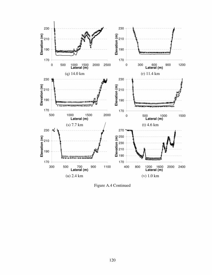
120
170
190
210
230
0 500 1000 1500 2000 2500Lateral (m)
Ele
vati
on
(m
)
170
190
210
230
0 300 600 900 1200Lateral (m)
Ele
vati
on
(m
)
(q) 14.0 km (r) 11.4 km
170
190
210
230
500 1000 1500 2000
Lateral (m)
Ele
va
tio
n (
m)
170
190
210
230
0 500 1000 1500Lateral (m)
Ele
vati
on
(m
)
(s) 7.7 km (t) 4.6 km
170
190
210
230
300 500 700 900 1100Lateral (m)
Ele
va
tio
n (
m)
170
190
210
230
250
270
400 800 1200 1600 2000 2400Lateral (m)
Ele
vati
on
(m
)
(u) 2.4 km (v) 1.0 km
Figure A.4 Continued

121
230
250
270
290
310
0 200 400 600 800Lateral (m)
Ele
vati
on
(m
)
Initial bed (MAY 2003)Surveyed (OCT 2006)Steady_OP1 (OCT 2006)Unsteady_OP1 (OCT 2006)
220
240
260
280
0 100 200 300Lateral (m)
Ele
vati
on
(m
)
(a) 101.6 km above the Xiaolangdi Dam (b) 88.5 km
210
230
250
270
0 200 400 600Lateral (m)
Ele
vati
on
(m
)
200
220
240
260
0 200 400 600Lateral (m)
Ele
vati
on
(m
)
(c) 80.2 km (d) 72.1 km
200
220
240
260
0 200 400 600 800Lateral (m)
Ele
vati
on
(m
)
200
220
240
260
500 1000 1500 2000 2500Lateral (m)
Ele
vati
on
(m
)
(e) 64.8 km (f) 57.0 km
200
220
240
260
0 500 1000 1500 2000 2500Lateral (m)
Ele
vati
on
(m
)
200
220
240
260
0 500 1000 1500Lateral (m)
Ele
vati
on
(m
)
(g) 55.0 km (h) 53.4 km
Figure A.5 Comparison of measurement and GSTARS4 simulation (Steady_OP1 and
Unsteady_OP1), in October 2006

122
200
220
240
260
0 500 1000 1500Lateral (m)
Ele
vati
on
(m
)
200
220
240
260
0 500 1000Lateral (m)
Ele
va
tio
n (
m)
(i) 50.2 km (j) 43.0 km
190
210
230
250
0 200 400 600 800Lateral (m)
Ele
vati
on
(m
)
190
210
230
250
500 1000 1500
Lateral (m)E
levati
on
(m
)
(k) 39.5 km (l) 36.3 km
190
210
230
250
0 300 600 900 1200Lateral (m)
Ele
vati
on
(m
)
180
200
220
240
0 200 400 600Lateral (m)
Ele
vati
on
(m
)
(m) 33.5 km (n) 27.2 km
180
200
220
240
500 1000 1500 2000 2500Lateral (m)
Ele
vati
on
(m
)
170
190
210
230
0 500 1000 1500 2000Lateral (m)
Ele
va
tio
n (
m)
(o) 22.1 km (p) 18.7 km
Figure A.5 Continued
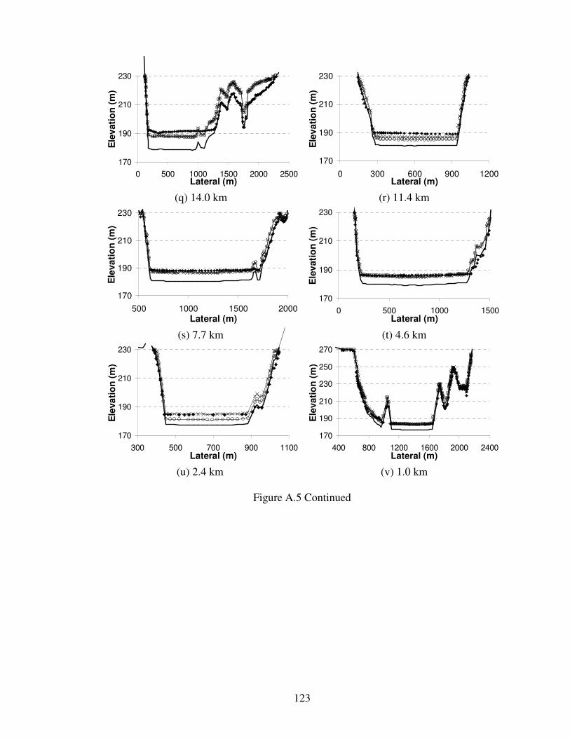
123
170
190
210
230
0 500 1000 1500 2000 2500Lateral (m)
Ele
vati
on
(m
)
170
190
210
230
0 300 600 900 1200Lateral (m)
Ele
vati
on
(m
)
(q) 14.0 km (r) 11.4 km
170
190
210
230
500 1000 1500 2000
Lateral (m)
Ele
va
tio
n (
m)
170
190
210
230
0 500 1000 1500Lateral (m)
Ele
vati
on
(m
)
(s) 7.7 km (t) 4.6 km
170
190
210
230
300 500 700 900 1100Lateral (m)
Ele
va
tio
n (
m)
170
190
210
230
250
270
400 800 1200 1600 2000 2400Lateral (m)
Ele
vati
on
(m
)
(u) 2.4 km (v) 1.0 km
Figure A.5 Continued

124
APPENDIX B
Simulated Steady Flow Reservoir Operation Type 2 (Steady_OP2), Unsteady Flow
Reservoir Operation Type 2 (Unsteady_OP2), and Measured Cross Section Geometry

125
230
250
270
290
310
0 200 400 600 800Lateral (m)
Ele
vati
on
(m
)
Initial bed (MAY 2003)Surveyed (OCT 2003)Steady_OP2 (OCT 2003)Unsteady_OP2 (OCT 2003)
220
240
260
280
0 100 200 300Lateral (m)
Ele
vati
on
(m
)
(a) 101.6 km above the Xiaolangdi Dam (b) 88.5 km
210
230
250
270
0 200 400 600Lateral (m)
Ele
vati
on
(m
)
200
220
240
260
0 200 400 600Lateral (m)
Ele
vati
on
(m
)
(c) 80.2 km (d) 72.1 km
200
220
240
260
0 200 400 600 800Lateral (m)
Ele
vati
on
(m
)
200
220
240
260
500 1000 1500 2000 2500Lateral (m)
Ele
vati
on
(m
)
(e) 64.8 km (f) 57.0 km
200
220
240
260
0 500 1000 1500 2000 2500Lateral (m)
Ele
vati
on
(m
)
200
220
240
260
0 500 1000 1500Lateral (m)
Ele
vati
on
(m
)
(g) 55.0 km (h) 53.4 km
Figure B.1 Comparison of measurement and GSTARS4 simulation (Steady_OP2 and
Unsteady_OP2), in October 2003

126
200
220
240
260
0 500 1000 1500Lateral (m)
Ele
vati
on
(m
)
200
220
240
260
0 500 1000Lateral (m)
Ele
va
tio
n (
m)
(i) 50.2 km (j) 43.0 km
190
210
230
250
0 200 400 600 800Lateral (m)
Ele
vati
on
(m
)
190
210
230
250
500 1000 1500
Lateral (m)E
levati
on
(m
)
(k) 39.5 km (l) 36.3 km
190
210
230
250
0 300 600 900 1200Lateral (m)
Ele
vati
on
(m
)
180
200
220
240
0 200 400 600Lateral (m)
Ele
vati
on
(m
)
(m) 33.5 km (n) 27.2 km
180
200
220
240
500 1000 1500 2000 2500Lateral (m)
Ele
vati
on
(m
)
170
190
210
230
0 500 1000 1500 2000Lateral (m)
Ele
va
tio
n (
m)
(o) 22.1 km (p) 18.7 km
Figure B.1 Continued
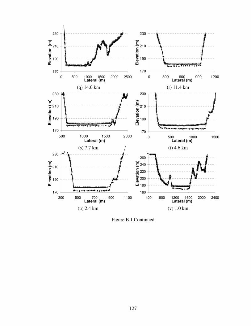
127
170
190
210
230
0 500 1000 1500 2000 2500Lateral (m)
Ele
vati
on
(m
)
170
190
210
230
0 300 600 900 1200Lateral (m)
Ele
vati
on
(m
)
(q) 14.0 km (r) 11.4 km
170
190
210
230
500 1000 1500 2000
Lateral (m)
Ele
va
tio
n (
m)
170
190
210
230
0 500 1000 1500Lateral (m)
Ele
va
tio
n (
m)
(s) 7.7 km (t) 4.6 km
170
190
210
230
300 500 700 900 1100Lateral (m)
Ele
va
tio
n (
m)
160
180
200
220
240
260
400 800 1200 1600 2000 2400Lateral (m)
Ele
vati
on
(m
)
(u) 2.4 km (v) 1.0 km
Figure B.1 Continued

128
230
250
270
290
310
0 200 400 600 800Lateral (m)
Ele
vati
on
(m
)
Initial bed (MAY 2003)Surveyed (MAY 2004)Steady_OP2 (MAY 2004)Unsteady_OP2 (MAY 2004)
220
240
260
280
0 100 200 300Lateral (m)
Ele
vati
on
(m
)
(a) 101.6 km above the Xiaolangdi Dam (b) 88.5 km
210
230
250
270
0 200 400 600Lateral (m)
Ele
vati
on
(m
)
200
220
240
260
0 200 400 600Lateral (m)
Ele
vati
on
(m
)
(c) 80.2 km (d) 72.1 km
200
220
240
260
0 200 400 600 800Lateral (m)
Ele
vati
on
(m
)
200
220
240
260
500 1000 1500 2000 2500Lateral (m)
Ele
vati
on
(m
)
(e) 64.8 km (f) 57.0 km
200
220
240
260
0 500 1000 1500 2000 2500Lateral (m)
Ele
vati
on
(m
)
200
220
240
260
0 500 1000 1500Lateral (m)
Ele
vati
on
(m
)
(g) 55.0 km (h) 53.4 km
Figure B.2 Comparison of measurement and GSTARS4 simulation (Steady_OP2 and
Unsteady_OP2), in May 2004

129
200
220
240
260
0 500 1000 1500Lateral (m)
Ele
vati
on
(m
)
200
220
240
260
0 500 1000Lateral (m)
Ele
va
tio
n (
m)
(i) 50.2 km (j) 43.0 km
190
210
230
250
0 200 400 600 800Lateral (m)
Ele
vati
on
(m
)
190
210
230
250
500 1000 1500
Lateral (m)E
levati
on
(m
)
(k) 39.5 km (l) 36.3 km
190
210
230
250
0 300 600 900 1200Lateral (m)
Ele
vati
on
(m
)
180
200
220
240
0 200 400 600Lateral (m)
Ele
vati
on
(m
)
(m) 33.5 km (n) 27.2 km
180
200
220
240
500 1000 1500 2000 2500Lateral (m)
Ele
vati
on
(m
)
170
190
210
230
0 500 1000 1500 2000Lateral (m)
Ele
va
tio
n (
m)
(o) 22.1 km (p) 18.7 km
Figure B.2 Continued

130
170
190
210
230
0 500 1000 1500 2000 2500Lateral (m)
Ele
vati
on
(m
)
170
190
210
230
0 300 600 900 1200Lateral (m)
Ele
vati
on
(m
)
(q) 14.0 km (r) 11.4 km
170
190
210
230
500 1000 1500 2000
Lateral (m)
Ele
va
tio
n (
m)
170
190
210
230
0 500 1000 1500Lateral (m)
Ele
va
tio
n (
m)
(s) 7.7 km (t) 4.6 km
170
190
210
230
300 500 700 900 1100Lateral (m)
Ele
va
tio
n (
m)
170
190
210
230
250
270
400 800 1200 1600 2000 2400Lateral (m)
Ele
vati
on
(m
)
(u) 2.4 km (v) 1.0 km
Figure B.2 Continued

131
230
250
270
290
310
0 200 400 600 800Lateral (m)
Ele
vati
on
(m
)
Initial bed (MAY 2003)Surveyed (OCT 2004)Steady_OP2 (OCT 2004)Unsteady_OP2 (OCT 2004)
220
240
260
280
0 100 200 300Lateral (m)
Ele
vati
on
(m
)
(a) 101.6 km above the Xiaolangdi Dam (b) 88.5 km
210
230
250
270
0 200 400 600Lateral (m)
Ele
vati
on
(m
)
200
220
240
260
0 200 400 600Lateral (m)
Ele
vati
on
(m
)
(c) 80.2 km (d) 72.1 km
200
220
240
260
0 200 400 600 800Lateral (m)
Ele
vati
on
(m
)
200
220
240
260
500 1000 1500 2000 2500Lateral (m)
Ele
vati
on
(m
)
(e) 64.8 km (f) 57.0 km
200
220
240
260
0 500 1000 1500 2000 2500Lateral (m)
Ele
vati
on
(m
)
200
220
240
260
0 500 1000 1500Lateral (m)
Ele
vati
on
(m
)
(g) 55.0 km (h) 53.4 km
Figure B.3 Comparison of measurement and GSTARS4 simulation (Steady_OP2 and
Unsteady_OP2), in October 2004

132
200
220
240
260
0 500 1000 1500Lateral (m)
Ele
vati
on
(m
)
200
220
240
260
0 500 1000Lateral (m)
Ele
va
tio
n (
m)
(i) 50.2 km (j) 43.0 km
190
210
230
250
0 200 400 600 800Lateral (m)
Ele
vati
on
(m
)
190
210
230
250
500 1000 1500
Lateral (m)E
levati
on
(m
)
(k) 39.5 km (l) 36.3 km
190
210
230
250
0 300 600 900 1200Lateral (m)
Ele
vati
on
(m
)
180
200
220
240
0 200 400 600Lateral (m)
Ele
vati
on
(m
)
(m) 33.5 km (n) 27.2 km
180
200
220
240
500 1000 1500 2000 2500Lateral (m)
Ele
vati
on
(m
)
170
190
210
230
0 500 1000 1500 2000Lateral (m)
Ele
va
tio
n (
m)
(o) 22.1 km (p) 18.7 km
Figure B.3 Continued

133
170
190
210
230
0 500 1000 1500 2000 2500Lateral (m)
Ele
vati
on
(m
)
170
190
210
230
0 300 600 900 1200Lateral (m)
Ele
vati
on
(m
)
(q) 14.0 km (r) 11.4 km
170
190
210
230
500 1000 1500 2000
Lateral (m)
Ele
va
tio
n (
m)
170
190
210
230
0 500 1000 1500Lateral (m)
Ele
va
tio
n (
m)
(s) 7.7 km (t) 4.6 km
170
190
210
230
300 500 700 900 1100Lateral (m)
Ele
va
tio
n (
m)
170
190
210
230
250
270
400 800 1200 1600 2000 2400Lateral (m)
Ele
vati
on
(m
)
(u) 2.4 km (v) 1.0 km
Figure B.3 Continued

134
230
250
270
290
310
0 200 400 600 800Lateral (m)
Ele
vati
on
(m
)
Initial bed (MAY 2003)Surveyed (NOV 2005)Steady_OP2 (NOV 2005)Unsteady_OP2 (NOV 2005)
220
240
260
280
0 100 200 300Lateral (m)
Ele
vati
on
(m
)
(a) 101.6 km above the Xiaolangdi Dam (b) 88.5 km
210
230
250
270
0 200 400 600Lateral (m)
Ele
vati
on
(m
)
200
220
240
260
0 200 400 600Lateral (m)
Ele
vati
on
(m
)
(c) 80.2 km (d) 72.1 km
200
220
240
260
0 200 400 600 800Lateral (m)
Ele
vati
on
(m
)
200
220
240
260
500 1000 1500 2000 2500Lateral (m)
Ele
vati
on
(m
)
(e) 64.8 km (f) 57.0 km
200
220
240
260
0 500 1000 1500 2000 2500Lateral (m)
Ele
vati
on
(m
)
200
220
240
260
0 500 1000 1500Lateral (m)
Ele
vati
on
(m
)
(g) 55.0 km (h) 53.4 km
Figure B.4 Comparison of measurement and GSTARS4 simulation (Steady_OP2 and
Unsteady_OP2), in November 2005

135
200
220
240
260
0 500 1000 1500Lateral (m)
Ele
vati
on
(m
)
200
220
240
260
0 500 1000Lateral (m)
Ele
va
tio
n (
m)
(i) 50.2 km (j) 43.0 km
190
210
230
250
0 200 400 600 800Lateral (m)
Ele
vati
on
(m
)
190
210
230
250
500 1000 1500
Lateral (m)E
levati
on
(m
)
(k) 39.5 km (l) 36.3 km
190
210
230
250
0 300 600 900 1200Lateral (m)
Ele
vati
on
(m
)
180
200
220
240
0 200 400 600Lateral (m)
Ele
vati
on
(m
)
(m) 33.5 km (n) 27.2 km
180
200
220
240
500 1000 1500 2000 2500Lateral (m)
Ele
vati
on
(m
)
170
190
210
230
0 500 1000 1500 2000Lateral (m)
Ele
va
tio
n (
m)
(o) 22.1 km (p) 18.7 km
Figure B.4 Continued

136
170
190
210
230
0 500 1000 1500 2000 2500Lateral (m)
Ele
vati
on
(m
)
170
190
210
230
0 300 600 900 1200Lateral (m)
Ele
vati
on
(m
)
(q) 14.0 km (r) 11.4 km
170
190
210
230
500 1000 1500 2000
Lateral (m)
Ele
va
tio
n (
m)
170
190
210
230
0 500 1000 1500Lateral (m)
Ele
va
tio
n (
m)
(s) 7.7 km (t) 4.6 km
170
190
210
230
300 500 700 900 1100Lateral (m)
Ele
va
tio
n (
m)
170
190
210
230
250
270
400 800 1200 1600 2000 2400Lateral (m)
Ele
vati
on
(m
)
(u) 2.4 km (v) 1.0 km
Figure B.4 Continued

137
230
250
270
290
310
0 200 400 600 800Lateral (m)
Ele
vati
on
(m
)
Initial bed (MAY 2003)Surveyed (OCT 2006)Steady_OP2 (OCT 2006)Unsteady_OP2 (OCT 2006)
220
240
260
280
0 100 200 300Lateral (m)
Ele
vati
on
(m
)
(a) 101.6 km above the Xiaolangdi Dam (b) 88.5 km
210
230
250
270
0 200 400 600Lateral (m)
Ele
vati
on
(m
)
200
220
240
260
0 200 400 600Lateral (m)
Ele
vati
on
(m
)
(c) 80.2 km (d) 72.1 km
200
220
240
260
0 200 400 600 800Lateral (m)
Ele
vati
on
(m
)
200
220
240
260
500 1000 1500 2000 2500Lateral (m)
Ele
vati
on
(m
)
(e) 64.8 km (f) 57.0 km
200
220
240
260
0 500 1000 1500 2000 2500Lateral (m)
Ele
vati
on
(m
)
200
220
240
260
0 500 1000 1500Lateral (m)
Ele
vati
on
(m
)
(g) 55.0 km (h) 53.4 km
Figure B.5 Comparison of measurement and GSTARS4 simulation (Steady_OP2 and
Unsteady_OP2), in October 2006
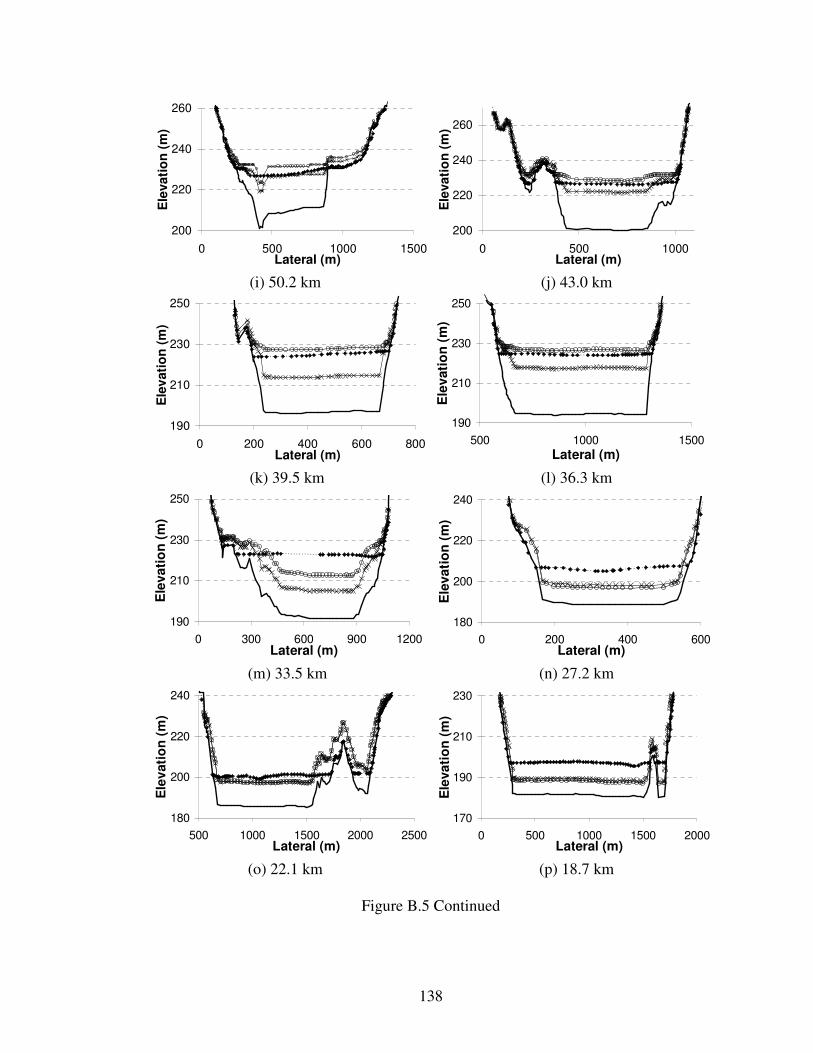
138
200
220
240
260
0 500 1000 1500Lateral (m)
Ele
vati
on
(m
)
200
220
240
260
0 500 1000Lateral (m)
Ele
va
tio
n (
m)
(i) 50.2 km (j) 43.0 km
190
210
230
250
0 200 400 600 800Lateral (m)
Ele
vati
on
(m
)
190
210
230
250
500 1000 1500
Lateral (m)E
levati
on
(m
)
(k) 39.5 km (l) 36.3 km
190
210
230
250
0 300 600 900 1200Lateral (m)
Ele
vati
on
(m
)
180
200
220
240
0 200 400 600Lateral (m)
Ele
vati
on
(m
)
(m) 33.5 km (n) 27.2 km
180
200
220
240
500 1000 1500 2000 2500Lateral (m)
Ele
vati
on
(m
)
170
190
210
230
0 500 1000 1500 2000Lateral (m)
Ele
va
tio
n (
m)
(o) 22.1 km (p) 18.7 km
Figure B.5 Continued

139
170
190
210
230
0 500 1000 1500 2000 2500Lateral (m)
Ele
vati
on
(m
)
170
190
210
230
0 300 600 900 1200Lateral (m)
Ele
vati
on
(m
)
(q) 14.0 km (r) 11.4 km
170
190
210
230
500 1000 1500 2000
Lateral (m)
Ele
va
tio
n (
m)
170
190
210
230
0 500 1000 1500Lateral (m)
Ele
va
tio
n (
m)
(s) 7.7 km (t) 4.6 km
170
190
210
230
300 500 700 900 1100Lateral (m)
Ele
va
tio
n (
m)
170
190
210
230
250
270
400 800 1200 1600 2000 2400Lateral (m)
Ele
vati
on
(m
)
(u) 2.4 km (v) 1.0 km
Figure B.5 Continued