dissertation paper - finsys.rau.rofinsys.rau.ro/docs/15-msc-rebedia.pdf · complex nonlinear...

THE ACADEMY OF ECONOMIC STUDIES

DOCTORAL SCHOOL OF FINANCE AND BANKING

DISSERTATION PAPER

SUPERVISOR:

PhD. Professor MOISA ALTAR

MSc STUDENT:

REBEDIA C VIORELA MARINELA

Bucharest,

2014

THE ACADEMY OF ECONOMIC STUDIES

DOCTORAL SCHOOL OF FINANCE AND BANKING

Complex nonlinear dynamics of

financial time series. An empirical

analysis using chaos theory

SUPERVISOR:

PhD. Professor MOISA ALTAR

MSc STUDENT:

REBEDIA C VIORELA MARINELA

Bucharest,

2014

CONTENT

ABSTRACT ................................................................................................................................. 8

I. INTRODUCTION ................................................................................................................ 5

II. LITERATURE REVIEW ..................................................................................................... 8

III. EMPIRICAL METHODOLOGY FOR THE ANALYSIS .................................................. 10

3.1. Metric Tools ..................................................................................................................... 10

3.1.1. The BDS test ...................................................................................................................... 10

3.1.2. Rescaled range analysis and Hurst exponent ................................................................. 12

3.2. Topological tests: Recurrence Analysis ............................................................................ 13

3.2.1. Recurrence Plot ................................................................................................................. 14

3.2.2. Recurrence Quantification Analysis ................................................................................ 19

IV. AN EMPIRICAL ANALYSIS USING CHAOS THEORY ................................................. 21

4.1. Data ................................................................................................................................. 21

4.2. Empirical results .............................................................................................................. 21

4.2.1. The BDS test results .......................................................................................................... 26

4.2.2. The Rescaled Range analysis results ............................................................................... 37

4.2.3. The Rcurrence Analysis results ....................................................................................... 38

CONCLUSIONS ........................................................................................................................ 43

REFERENCES .......................................................................................................................... 45

APPENDIX ................................................................................................................................ 48

ABSTRACT

This paper presents an effort to implement metric and topological tools, to test for the

presence of nonlinear dependence and deterministic chaos, in the returns series for eight stock

market indices. Chaos theory might be useful in explaining the dynamics of financial markets,

since chaotic models are capable of exhibiting behaviour similar to that observed in real

financial data. In this context, the scope of this research is to provide an insight into the role that

nonlinearities and, in particular, chaos theory may play in explaining the dynamics of financial

markets.

Based on the following chaos tests: BDS test, Hurst exponent using R/S analysis,

Recurrence Plots and Recurrence Quantification Analysis, the overall result of this study

suggests that the returns series do not follow a random walk process. Rather it appears that the

daily returns are serially correlated and the estimated Hurst exponents are indicative of marginal

persistence. Result from the test of independence on filtered residuals suggests that the existence

of nonlinear dependence, at least to some extent, can be attributed to the presence of conditional

heteroskedasticity. It appears, therefore, that GARCH-type models can adequately explain some,

but not all, of the observed nonlinear dependence in the data. Further, we find evidence to

support the proposition that returns are generated by a chaotic system in five out of eight cases.

Presence of chaos in market indices implies that profitable nonlinearity based trading rules may

exist at least in the short-run. Finally, fairly contrary to the findings of previous studies, rejection

of random walk hypothesis offers some possibility of returns predictability.

5

I. INTRODUCTION

The main aim of this study is to investigate the presence of nonlinear dependence and

deterministic chaos in daily returns on eight stock market indices by contrasting the random walk

hypothesis with chaotic dynamics. More specifically, I attempt to test for long-range dependence,

nonlinear structure and chaos in both developed and emerging markets by investigating if daily

returns series of stock market indices show any sign of biased-random walk and chaotic behavior.

Over the years, movements in stock prices have fascinated not only the speculative traders,

but also the academicians and policy makers. For the last four decades, the efficient market

hypothesis (EMH) has been the dominant theory in the financial markets. Many studies have been

conducted to test the theory. Under the EMH, stock returns processes should be random. Market

efficiency idea mentions that prices fully reflect all information and price movements do not follow

any patterns or trends. That is, past price movements cannot be used to predict the future price

movements but follow what is known as a random walk, an intrinsically unpredictable pattern. The

idea that stock price variations are generated by a random process with no long-term memory has

long been prominent in international and quantitative finance research. Under this approach, it was

believed that stock returns are independent and identically distributed (IID) random variables.

Presence of this traditional belief is also reflected in the assumptions of prominent asset pricing

theories such as Sharpe–Lintner model of market equilibrium and the Black–Scholes theory of

option pricing. The assertion of random walk seemed indisputable not only on empirical

justifications but also for apparently strong theoretical reasons - namely, consistency with the

efficient market paradigm (Abhyankar, Copeland, & Wong, 1997). Validity of the efficient market

hypothesis in real world actually precludes the possibility that market players can generate higher

returns from using trading rules. Interestingly, empirical findings of earlier studies have, by and

large, confirmed the validity of random walk (Fama, 1970).

However, the pioneering work of Mandelbrot (1963) challenged this classical conviction by

establishing that increments of stock prices or return variations did indeed possess a long-memory,

which may be best described by fractional Brownian motion. Further, Rogers (1997) countered the

traditional random walk hypothesis much strongly by establishing that under the condition of

fractional Brownian motion (when Hurst exponent H≠0.5), arbitrage opportunities and monetary

6

profits can be generated from financial markets without taking any substantial risk, which is

certainly anathema to the prominent financial theory. Following this line of argument, an increasing

number of studies using chaotic and nonlinear estimation techniques for modeling financial data

have highlighted the nonlinear deterministic behaviour of stock prices. These findings strongly and

collectively suggest that stock prices may be more predictable than it was previously thought under

the random walk approach. In other words, adherents of biased-random walk approach believe that

seemingly random stock price and returns sequences may not be random and there are reasons to

believe that they may arise from deterministic nonlinear dynamical systems, instead.

The discovery of nonlinear dependence and deterministic chaos in financial data has altered

our traditional view of the erratic behaviour of financial variables by providing an entirely different

perspective to analyze financial data moving well beyond the realm of linear paradigm and random

walk approach of stock price movements. Nonlinear deterministic systems with a few degrees of

freedom can create output signals that appear complex and mimic stochastic signals from the point

of view of conventional time series analysis but are chaotic. Chaotic systems are complex systems

which belong to the class of deterministic dynamical systems. They are detected and used in a lot of

fields for control or forecasting. Deterministic chaos has been rigorously and extensively studied by

mathematicians and other scientists. It is almost impossible to give a precise mathematical

definition of deterministic chaos that encapsulates everything in the diverse literature. Chaos is said

to be an irregular oscillatory process broadly characterized by three conditions: nonlinearity, fractal

attractor, and sensitive dependence on initial conditions (SDIC) (Faggini, 2011). A unique feature of

chaotic system is that it can generate large and apparently random fluctuations, quite similar to the

sudden ups and downs sometimes seen in the stock market. Interestingly, stochastic models explain

that many of these sudden fluctuations are actually caused by external random shocks. However, in

a chaotic system these abrupt fluctuations are considered to be internally generated as part of the

deterministic process (Gilmore, 1996). This makes a strong case for the application of chaotic

dynamic to model and explain nonlinearity in financial time series. Although chaos is highly

unpredictable, its deterministic nature offers good opportunity for profitable forecast at least in the

short-run. However, forecasting over long horizon is not possible mainly because of the SDIC

property of a chaotic system.

Researchers in economics and finance have been interested in testing nonlinear dependence

and chaos for almost three decades. A wide variety of reasons for this interest have been suggested,

7

including an attempt to improve the forecasting accuracy of linear time series models and to better

explain the dynamics of the underlying variables of interest using a richer class of models than that

permitted by limiting the set to the linear case. The issue of whether a financial series is indeed

chaotic may not be of great importance to a financial forecaster who is only interested in adjusting

dynamic trading strategies according to apparent predictability in time series. During these three

decades the search for chaos in economics has gradually became less enthusiastic, as little or no

empirical support for the presence of chaotic behaviours in economics has been found. The

literature did not provide a solid support for chaos as a consequence of the high noise level that

exists in most economic time series, and the relatively small sample sizes of data.

Against this background, in the present study I attempt to investigate nonlinear and chaotic

structure in daily returns series of market indices. The motivation for undertaking this study is not

only the dearth of research in this domain but also the potential implications of such a study for

players in these markets. Detection of a deterministic chaos would mean an opportunity for hedgers,

speculators as well as arbitrageurs to play the markets better.

This paper offers several contributions to the existing literature. Although there are many

studies on this issue, covering different sample periods and markets, but to my knowledge, this is

one of the first attempts to investigate chaotic structure in both developed and emerging markets.

The search for chaos in financial markets has been mostly restricted to stock markets and in too

developed countries. However given the very different institutional features of financial markets in

developing countries, it is important to explore the possibilities of such markets exhibiting chaotic

behavior. Financial markets in developing countries are less mature as compared to those in

developed countries, and the implications of complex nonlinear behavior could be significant for

traders, institutional investors for devising suitable trading strategies. Second, instead of performing

a direct test for chaos, I apply different techniques to investigate the underlying data generating

process. These tests will help investigate the adequacy of generally applied linear or nonlinear

econometric models for forecasting these financial time series. Finally, the study of chaotic dynamic

will help determine the degree of predictability and efficiency in financial markets.

The rest of the paper is organized as follows. Section 2 presents a brief review of literature.

Section 3 discusses empirical methodologies and provides a brief account of tests used in the study.

Section 4 presents empirical results. The final section provides concluding observations based on

the findings of the study.

8

II. LITERATURE REVIEW

The efficient market hypothesis and the random walk approach to explain the time series

behaviour of stock prices have been in the centre of attention for years. There are many studies

supporting the EMH in the literature (Kendall, 1953; Brealey, 1970; Cunningham, 1973; Brock,

1987). These studies on the United Kingdom and Canadian stock markets, based on the assumption

that stock market price changes are i.i.d., detect the weak form market efficiency and find no

evidence of chaos in macroeconomic time series.

However, the pioneering work of Mandelbrot (1963) challenged the random walk theory and

initiated a new debate by bringing the concept of long-memory and biased random walk into

perspective.

In 1965, Fama admitted that linear modeling techniques have limitations as they are not

sophisticated enough to capture complicated ―patterns‖ which chartists claim to see in stock prices.

The recent empirical literature has mainly focused on testing for the presence of long-

memory, nonlinear dependence and chaos in financial data by using new techniques and models

indicative of complex dynamics (Abhyankar, Copeland, and Wong, 1995; Abhyankar, 1997).

Although some studies have produced conflicting results, but now a broad consensus has

emerged that nonlinear structure in financial time series is a somewhat realistic phenomenon

(Brock, Hsieh, & LeBaron, 1992). The literature, especially after the earlier findings of nonlinear

dependence in returns by Hinich and Patterson (1985) and Frank and Stengos (1989), has seen many

such studies. In general, recent studies have consistently documented strong evidence of

nonlinearity in the returns of various assets. Studies applying tests based on nonlinear dynamics

have also concluded that residuals of filtered stock returns are not IID and, therefore, market returns

do not follow random walk process. While considering the case of long-memory, contrary to the

traditional belief, many recent studies have reported strong evidence of long-range dependence in

the returns of various assets (Cajueiro and Tabak, 2009; Helms et al., 1984). Using the classical

rescaled-range analysis, Howe et al. (1999) find strong evidence of long-range nonlinear

deterministic structure in the returns of the Japanese, Singaporean, Korean, and Taiwanese indices

with cycle length ranging from 3 to 4 years. However, contrary to these findings, Lo (1991),

9

Cheung and Lai (1995) and Jacobsen (1996) failed to find any evidence of long-range dependence

in stock returns for some European countries, the United States and Japan.

As far as the presence of nonlinear deterministic and chaotic structures in market returns are

concerned, the published evidence is rather mixed. For example, studies such as Frank and Stengos

(1989), Hsieh (1991), Blank (1991) and DeCoster, Labys, and Mitchell (1992), have found strong

evidence of nonlinear dependence and chaotic structure in economic and financial time series

whereas Kosfeld and Robe (2001) for German bank stock returns and Opong, Mulholland, Fox, and

Farahmand (1999) for London Financial Times Stock Exchange found that low order GARCH

models are sufficient to explain the existing nonlinearity in the data. Similarly, in his study Brooks

(1998) reported strong evidence of nonlinearity but failed to find any significant evidence of

deterministic chaos in the data. Scheinkman and LeBaron (1989) study U.S.A. weekly returns on

the Center for Research in Security Prices (CRSP) value-weighted index, employing the BDS

statistic, and find rather strong evidence of nonlinearity and some evidence of chaos. Brock, Hsieh

and LeBaron (1991) concluded that the evidence for the presence of deterministic low-dimensional

chaotic generators in economic and financial data is not very strong.

Nevertheless, some recent studies have documented encouraging evidence of chaos in

exchange rate data. For example, in their study Serletis and Gogas (1997) and Scarlat, Stan, and

Cristescu (2007) found consistent evidence of chaotic dynamics in various markets.

In a working paper, Wei and Leuthold (1998) looked at six agricultural futures markets—

corn, soybeans, wheat, hogs, coffee and sugar—and found that five of them (all except sugar) were

chaotic processes.

Andreou, Pavlides and Karytinos (2000) examined four major currencies against GRD and

found evidence of chaos in two out of four.

Panas and Ninni (2000) found strong evidence of chaos in daily oil products for the

Rotterdam and Mediterranean petroleum markets.

It is clear that while there is a broad consensus on the presence of nonlinear dependence in

market returns, the issue is still unsettled for chaos in financial data. Furthermore, there is hardly

any study on emerging markets to explain the time series behaviour of stock returns. Therefore, this

study attempts to fill this gap by providing some additional evidence from the emerging countries.

10

III. EMPIRICAL METHODOLOGY FOR THE ANALYSIS

The fast development of computer resources available to the scientist community and the

parallel growing bulk of theoretical knowledge about complex dynamics have allowed many

researches to look for nonlinear dynamics in data whose evolution linear ARMA models are unable

to explain in a satisfactory manner. The methods involved in Nonlinear Time Series Analysis can be

classified into metric, dynamical, and topological tools. The metric approach depends on the

computation of distances on the system's attractor, and it includes Grassberger-Procaccia correlation

dimension and BDS test. The dynamical approach deals with computing the way nearby orbits

diverge by means of estimating Lyapunov exponents. Topological methods are characterised by the

study of the organisation of the strange attractor, and they include recurrence plots.

In practice, various criteria and methods are used to detect nonlinear structure and chaos in

the data. Given that the study of chaos is relatively new in financial research, there is no single

commonly accepted statistical test to determine precisely the nature of nonlinearity and chaotic

structure in the data (Gilmore, 1996). A best alternative approach, therefore, would be to use all

available criteria for analyzing the behaviour of stock price or return time series. The tests applied in

this study are widely used in literature.

3.1. Metric Tools

3.1.1. The BDS test

Brock, Dechert, LeBaron, and Scheinkman (1996) developed a powerful test for

independence and identical distribution based on correlation function developed by Grassbeger and

Procaccia (1983). This test is also known as BDS test for nonlinear dependence between points on a

reconstructed attractor. The BDS test tests the null hypothesis of whiteness (IID observations)

against an unspecified alternative using a nonparametric technique.

In fact, BDS test is not considered to be a direct test for chaos. It is useful because it is a well

defined, and easy to apply test which has power against any type of structure in a series. This

feature can be viewed as both a cost and a benefit. On the one hand it can detect many types of

nonlinear dependence that might be missed by other tests. On the other hand, a rejection using this

11

test is not very informative. One extension of this test is to use it as a residual diagnostic, as a model

selection tool to obtain some information about what kind of dependency exists after removing

linear dependency from the data. However, it is possible to use the BDS test to indirectly search for

nonlinear dependence which is necessary but not sufficient condition for chaos. The test is applied

to residuals to check if the best-fit model for a given time series is a linear or nonlinear model.

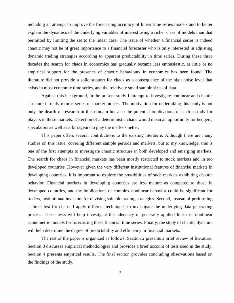
Under the null hypothesis of whiteness, the BDS statistic is given by:

√

where is an estimate of the standard deviation of C(N,m,ε) - C(N,1,ε)m

.

The correlation function asymptotically follows standard normal distribution N(0,1):

Moving from the hypothesis that a time series is IID, the BDS tests the null hypothesis that

, which is equivalent to the null hypothesis of whiteness against an

unspecified alternative.

Both positive as well as negative values of the test statistic are taken as an indication of non-

IID behaviour. BDS statistics takes a positive value if the probability of any two m-histories (xt,

xt+1,…, xt+m-1) and (xs, xs+1,……., xs+m-1) of being ―close‖ together is higher than that of mth power

of the any two points xt and xs. In other words, a significant and positive BDS statistics indicates

that certain patterns such as ―clustering‖ are too frequent compared to a true random process

whereas a significant and negative BDS test statistic indicates that certain patterns are too infrequent

compared to a true random process.

If series are IID so that linear or even conditional heteroskedasticity can describe the

relations between data, chaotic tests will not be required. However, if this is not the case,

investigating the main properties of chaoticity should not be disregarded.

Because it is based on the correlation dimension, the BDS test suffers from the same

limitations. In particular, its performance depends on the size of data sets (N) and ε, even though

Brock (1991) showed how the statistics of this test are correctly approximated in finite samples if:

- the number of data N is greater than 500.

- ε lies between 0.5σ and 2σ, where σ is the standard deviation of the series.

- the embedding dimension m is lower than N/200.

12

3.1.2. Rescaled range analysis and Hurst exponent

The EMH assumes that all investors immediately react to the new information. Some recent

studies, however, argue that this is not always true in the market. For example, Peters (1994) argues

that most people do not react immediately on the arrival of new information. Instead they wait for

confirming the information and do not react until a trend is clearly visible in the market. Therefore,

there will be an uneven assimilation of information and this will cause stock price movements to

follow a biased-random walk rather than pure random walk. If this is true, the possibility of biased-

random walk implies that there is memory or temporal dependence in the underlying series.

In literature, a tool extensively used for testing long-term memory and fractality of a time

series is the R/S analysis. In the present study, we broadly follow Peters (1994) to conduct R/S

analysis.

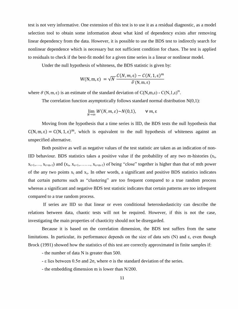
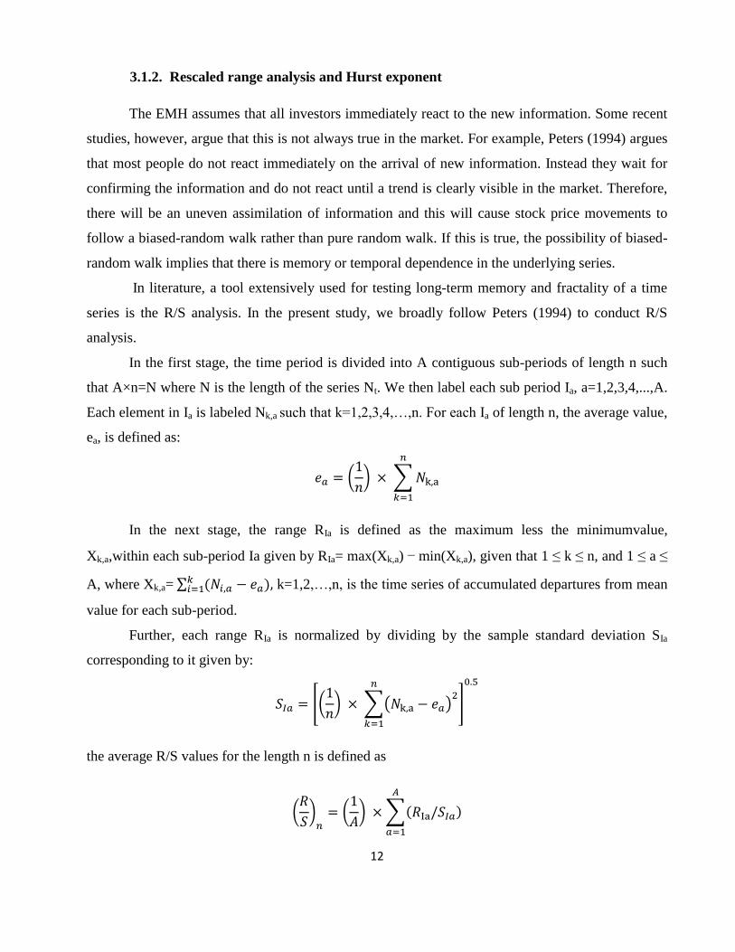
In the first stage, the time period is divided into A contiguous sub-periods of length n such

that A×n=N where N is the length of the series Nt. We then label each sub period Ia, a=1,2,3,4,...,A.

Each element in Ia is labeled Nk,a such that k=1,2,3,4,…,n. For each Ia of length n, the average value,

ea, is defined as:

(

) ∑

In the next stage, the range RIa is defined as the maximum less the minimumvalue,

Xk,a,within each sub-period Ia given by RIa= max(Xk,a) − min(Xk,a), given that 1 ≤ k ≤ n, and 1 ≤ a ≤

A, where Xk,a= ∑ k=1,2,…,n, is the time series of accumulated departures from mean

value for each sub-period.

Further, each range RIa is normalized by dividing by the sample standard deviation SIa

corresponding to it given by:

[(

) ∑( )

]

the average R/S values for the length n is defined as

(

) (

) ∑

13

Now the final stage involves applying an ordinary least square (OLS) regression with log(n)

as the independent variable and (R/S)n as the dependent variable. Hurst (1951) show that R/S could

be estimated by the following empirical relationship, generally referred to as Hurst's Empirical Law:

(R/S) = a (N)H

where a is a constant and H equals the Hurst exponent. Now after obtaining logs of both sides of the

Hurst's equation, we obtain:

log (R/S) = H × log (N) + log (a).

The Hurst exponent, H, is the slope coefficient obtained from this regression. For the

classification of time series, the Hurst exponent can be interpreted as follows:

- a Hurst exponent of 0.5 indicates that the series behaves in a manner consistent with the

random walk or nondeterministic process;

- an H of greater than 0.5 indicates ‗persistence‘ or trend-reinforcing series;

- an H of less than 0.5 indicates ‗antipersistence‘ or ergodic series.

3.2. Topological tests: Recurrence Analysis

The failure to find convincing evidence for chaos in economic and financial time series

redirected the interest to additional tests that work with small data sets and that are robust against

noise. This goal seems to be reached by topological tools based on topological invariant testing

procedure. Compared to the existing metric and dynamical classes of testing procedures, these tools

could be better suited to testing for chaos in financial and economic time series and to provide

information about the underlying system responsible for chaotic behaviour.

The topological approach to testing for chaos has origins as far back as Poincaré (1892) and

attempts to determine how the unstable periodic orbits of the strage attractor are interwined.

Topological tools are characterised by studying the organisation of the strange attractor because

they exploit an essential property of a chaotic system, i.e. the tendency of the time series to nearly,

although never exactly, repeat itself over time. This property is known as the recurrence property.

The processes of stretching and compression are responsible for organising the strange

attractor in a unique way and if one can determine how the unsable periodic orbits are organised, we

can identify the stretching and compressing mechanisms responsible for the creation of the strange

14

attractor. Once these mechanisms have been identified, a geometric model can be constructed,

which describes how to model the stretching and squeezing mechanisms responsible for generating

the original time series. That is to say, topological tests may not only detect the presence of chaos

(the only information provided by the metric class of tests), but can also provide information about

the underlying system responsible for the chaotic behavior.

Unlike the metric approach, as the topological method preserves time ordering, that‘s the

temporal correlation in a time series in addition to the spatial structure of the data, where evidence

of chaos is found, the researcher may proceed to characterise the underlying process in a

quantitative way.

An example of these topological tests is Recurrence Analysis. Recurrence Analysis is

composed by the Recurrence Plot (RP) developed by Ekmann (1987), the graphical tool that

evaluates the temporal and phase space distance, designed to locate hidden recurring patterns,

nonstationarity and structural changes, and Recurrence Quantification Analysis (RQA), the

statistical quantification of RP.

3.2.1. Recurrence Plot

Recurrence plots are graphical devices specially suited to detect hidden dynamical patterns

and nonlinearities in data. With recurrence plots, one can also graphically detect structural changes

in data or see similarities in patterns across the time series under study. The fundamental

assumption underlying the idea of the recurrence plots is that an observable time series (a sequence

of observations) is the realization of some dynamical process, the interaction of the relevant

variables over time.

As remarkable as it seems, it has been proven mathematically that one can recreate a

topologically equivalent picture of the original multidimensional system behavior by using the time

series of a single observable variable (Takens, 1981). The basic idea is that the effect of all the other

(unobserved) variables is already reflected in the series of the observed output. Furthermore, the

rules that govern the behavior of the original system can be recovered from its output.

The starting point of the RPs is based on the time delay method through which the original

series is transformed into a set of m-histories. The Recurrence Plot is a two dimensional

representation of those m-histories whose coordinates are the present and lagged values of the

series.

15

The original series is transformed into an m-dimensional system that, depending on the

fulfilment of certain conditions, is topologically equivalent to the original system from which the

series was supposedly determined. The one-dimensional signal is expanded into an m-dimensional

phase space by substituting each observation with vector:

{ }

As a result, we have a series of vectors:

{ }

where N is the number of observations, m is the embedding dimension and d is the delay time.

Time delay determines the time separation or predictability of the components in the

reconstructed vectors of the system state. It should be chosen so that the elements in the embedding

vectors are no longer correlated, thus subsequent analysis would reveal spatial (or geometrical)

structures.

The embedding dimension determines the number of the components in the reconstructed

vector of the system state. It should be large enough to unfold the system trajectories from self-

overlaps, but not too large as the noise will amplify.

If the unknown system that generated { } is N-dimensional, and provided that

embedding dimension, if m ≥ 2n+1, the set of m-histories recreates the dynamics of the data-

generating system and can be used to analyse its dynamics. However, the sequence of embedded

vectors is useful only if parameters m and d are properly chosen by using appropriate methods.

Next, a symmetric matrix of distances (e.g., Euclidean distances) can be constructed by

computing distances between all pairs of embedded vectors. By using an appropriate norm and

fixing a threshold ε that determines if vectors x(i) and x(j) are sufficiently close together – distance

between them below or equal to ε - we obtain a recurrence matrix formally expressed as following:

‖ ‖ for i, j = M

where M = N-(m-1)d, H is the Heaviside function, and || || is a norm, generally Euclidian.

The matrix R consists of values 0 (no recurrence) and 1 (recurrence). More formally:

{ ‖ ‖

‖ ‖

16

The recurrence plot relates each distance of such a matrix to a colour (e.g., the larger is the

distance, the ―cooler" is the colour). Thus, the recurrence plot is a solid rectangular plot consisting

of pixels whose colours correspond to the magnitude of data values in a two-dimensional array and

whose coordinates correspond to the locations of the data values in the array. Generally dark colour

marks nonzero values, that is, short distances, and a light colour zero values, that is, the long

distance.

Both axes of the RP are time axes and show rightwards and upwards (convention). Vectors

compared with themselves necessarily compute to distances of zero, which means that by definition

the RP always has a black main diagonal line, the line of identity and it is symmetric with respect to

the main diagonal, i.e. Ri,j ≡ Rj,i.

This graphic tool shows different structures depending on the nature of the series under

study. In particular, it is capable of detecting the time recurrence patterns underlying deterministic

systems (whether they are chaotic or not). Non-chaotic deterministic systems exhibit very simple

regular structures, while the RPs of chaotic systems also show a certain regularity but with more

complex and denser features. On the other hand, the RPs obtained from purely random systems do

not show distinguishable patterns, appearing as a cloud of points with no apparent structure.

To illustrate the basic ideas behind RP some examples by Visual Recurrence Analysis

(VRA) are used. In VRA, a one-dimensional time series from a data file is expanded into a higher-

dimensional space, in which the dynamic of the underlying generator takes place. This is done using

a technique called ―delayed coordinate embedding‖, which recreates a phase space portrait of the

dynamical system under study from a single (scalar) time series. The idea of such reconstruction is

to capture the original system states at each time we have an observation of that system output.

The first recurrence plot that VRA shows can be a beautiful picture, but absolutely

uninformative. We must choose a suitable embedding dimension and an adequate time delay. To

choose the appropriate time delay, we can compute the ―average mutual information function‖, as

an alternative to the classical autocorrelation function; the latter detects linear correlations, but the

former is useful to detect both linear and non-linear correlations. The time delay should be chosen

such that the elements in embedding vectors are no longer correlated, thus subsequent analysis

would reveal spatial or geometrical structures. We can also use a procedure called ―false nearest

neighbours method" to find the optimal embedding dimension.

17

Once the dynamical system is reconstructed in a manner outlined above, a recurrence plot

can be used to show which vectors in the reconstructed space are close and far from each other. This

way one can visualize and study the motion of the system trajectories and infer some characteristics

of the dynamical system that generated the time series.

If the analysed time series is deterministic, then the recurrence plot shows short line

segments parallel to the main diagonal.

Figure 1. Lorenz attractor Figure 2. White noise

Figure 3. Sine wave

As an illustration, Figure 1 shows the recurrence plot from the (chaotic) Lorenz attractor, for

a time delay d = 17 (selected through the method of average mutual information) and an embedding

dimension m = 3 (selected through the false nearest neighbours method). Figure 2 shows the

recurrence plot from a Gaussian white noise, for d = 1 and m = 12 and figure 3 shows the recurrence

plot from a Sine wave, for d = 25 and m = 2. All figure have been attained using VRA.

18

Recurrent points in Figure 1 for the Lorenz attractor form distinct short diagonals parallel to

the main diagonal. The upward diagonal lines result from strings of vector patterns repeating

themselves multiple times down the dynamics. This type of recurrent structure indicates that the

dynamics is visiting the same region of an attractor at different times; therefore, the presence of

diagonal lines indicates that deterministic rules are present in the dynamics. The set of lines parallel

to the main diagonal is the signature of determinism.

Alternatively, in Figure 2, recurrence points for the white noise are simply distributed in a

homogeneous random pattern – a cloud of points, signifying that a random variable lacks of

deterministic structures.

Diagonal structures show (Figure 3) the range in which a piece of the trajectory is rather

close to another piece of the trajectory at different times. From the occurrence of lines parallel to the

diagonal in the recurrence plot, it can be seen how fast neighboured trajectories diverge in phase

space. These lines would not occur in a random as opposed to deterministic process. Thus, if the

analysed time series is chaotic, then the recurrence plot shows short segments parallel to the main

diagonal: chaotic behaviour causes very short diagonals, whereas deterministic behaviour causes

longer diagonals (Figure 1 vs. Figure 3).

This procedure has some advantages such as simplicity of implementation, robustness to

sample length, high dimensionality, noisy dynamics in the underlying equations of motion and

fewer prior requirements of the database used. RP analysis is independent of limiting constraints

such as data set size, noise, and stationarity; prewhitening of the data (linear filtering, detrending, or

transforming the data to conform to any particular distribution) is not necessary as stationarity is not

as essential like for the metric approach (Faggini, 2013).

Nevertheless some limitations are present. The first one is the construction of RPs and

obtaining the Recurrence Matrix (RM). Because they are carried out on the basis of the time delay

method, which requires previously fixing the values of the embedding dimension and the time

delay, the results obtained from the RP application are sensitive to the values chosen for these

parameters. The second one is the difficulty to interpret the graphical output of RP. Sometimes the

signature of determinism, the set of lines parallel to the main diagonal might not be so clear (e.g.,

the size of the lines being relatively short among a field of scattered recurrent points), i.e., the

recurrence plot could contain subtle patterns not easily ascertained by visual inspection; in this

context, Zbilut and Webber (1992) propose the so called recurrence quantification analysis (RQA).

19

3.2.2. Recurrence Quantification Analysis

The RQA considers that it is possible to quantify the information supplied by RP and, using

certain simple pattern recognition algorithms, to summarize the information in a set of indicators or

statistics. In this way more objective information than that which could be derived from a purely

visual analysis are obtained.

Considering that RP is symmetric, the set of indicators is obtained using the upper or lower

triangular part of RP excluding the main diagonal. The main indicators are recurrence rate,

determinism, averaged length of diagonal structures, entropy and trend.

Recurrence rate (REC): recurrence points percentage defined as:

where NREC is the number of recurrent points and NP is the total element of the recurrence matrix.

This variable can range from 0% (no recurrent points) to 100% (all points recurrent). Roughly

speaking REC is what is used to compute the correlation dimension of data.

Determinism rate (DET) is the ratio of recurrence points forming diagonal structures to all

recurrence points. DET measures the percentage of recurrent points forming line segments that are

parallel to the main diagonal and is calculated as

where NPD is the number of points on lines parallel to the main diagonal caused by the existence of

time correlation within the trajectory. Diagonal line segments must have a minimum length defined

by the line parameter.

The presence of such diagonal structuring in RM is assumed to be a distinctive feature of

deterministic structures, absence, instead, of randomness. DET is related with the determinism of

the system: the greater the number of points is on line segments, the greater the general dependence

of the series will be. Periodic signals (e.g. sine waves) will give very long diagonal lines, chaotic

signals (e.g. Hénon attractor) will give very short diagonal lines, and stochastic signals (e.g. random

numbers) will give no diagonal lines at all.

Maxline (MAXLINE) represents the averaged length of diagonal structures and indicates the

longest line segments that are parallel to the main diagonal. Unlike the %DET counts all the points

on the parallel lines equally regardless of their size, this indicator considers the length of the

20

different lines. This is a very important recurrence variable because it inversely scales with the the

largest positive Lyapunov exponent (Eckmann et al., 1987; Trulla et al., 1996). Positive Lyapunov

exponents gauge the rate at which trajectories diverge, and are the hallmark for dynamic chaos.

Thus, the shorter the linemax, the more chaotic (less stable) the signal.

Entropy (ENT) (Shannon entropy) measures the distribution of those line segments that are

parallel to the main diagonal and reflects the complexity of the deterministic structure in the system.

ENT is a measure of signal complexity and is calibrated in units of bits/bin. Individual histogram

bin probabilities are computed for each non-zero bin and then summed according to Shannon‘s

equation. A high ENT value indicates a large diversity in diagonal line lengths; low values indicate

small diversity in diagonal line lengths. For simple periodic systems in which all diagonal lines are

of equal length, the entropy would be expected to be 0.0 bins/bin.

The value trend (TREND) quantifies the degree of system stationarity. It measures the

paling of the patterns of RPs away from the main diagonal used for detecting drift and non-

stationarity in a time series. It is calculated as a slope of the %REC as a function of the

displacement of the main diagonal. If recurrent points are homogeneously distributed across the

recurrence plot, TND values will hover near zero units. If recurrent points are heterogeneously

distributed across the recurrence plot, TND values will deviate from zero units.

Laminarity (LAM) is analogous to %DET except that it measures the percentage of recurrent

points comprising vertical line structures rather than diagonal line structures. The line parameter

still governs the minimum length of vertical lines to be included.

Trapping time (TT) is simply the average length of vertical line structures.

21

IV. AN EMPIRICAL ANALYSIS USING CHAOS THEORY

4.1. Data

The empirical application in this paper is based on eight data sets representing the closing

prices of stock indices, selected from both developed countries and emerging countries, namely:

BET-C (Bucharest Stock Exchange - Romania), BUX (Budapest Stock Exchange - Hungary), DAX

(Frankfurt Stock Exchange - Germany), FTSE 100 (London Stock Exchange - United Kingdom),

FTSE MIB (Milan Stock Exchange - Italy), Nikkei 225 (Tokyo Stock Exchange - Janponia),

SOFIX (Sofia Stock Exchange - Bulgaria) and S&P 500 (New York Stock Exchange - USA).

The data used are on a daily basis covering the period January 2nd

, 2002 to May 22th

, 2014.

In the sample period are included 3232 observations. Missing data were replaced by the arithmetic

mean of the last two values available.

Based on the eight data sets collected, the prices were converted in daily returns. We apply

the following transformation to the raw data before conducting statistical tests:

Rit = ln(Pi,t) – ln(Pi,t-1)

where: Rit is the rate of ruturn of stock index i at time t;

Pi,t este is the close price of stock index i at time t.

This transformation implements an effective detrending of the series. This method also

provides an effective way to measure the continuously compounded rates of returns. For each set of

data we have a number of 3231 calculated returns.

In the analysis were used the following programs: Eviews7, Matlab R2013a and VRA 4.9.

4.2. Empirical results

First we analyzed the behavior of daily returns. In the table below we present the

characteristics of the data series.

The highest, and the lowest yield was obtained for the BUX index. If we compare the

standard deviations, the most risky is BUX index trading and the least risky is FTSE 100 index

trading.

22

Table 1. Descriptive statistics for daily returns

BET-C BUX DAX FTSE 100 FTSE

MIB

NIKKEI

225 SOFIX S&P 500

Mean 0.000585 0.000305 0.000196 0.0000829 -0.000140 0.0000977 0.000499 0.000153

Median 0.000571 0.000449 0.000724 -0.0000441 0.000446 0.000312 0.000465 0.000663

Maximum 0.108906 0.131777 0.107975 0.093842 0.108742 0.094941 0.083878 0.109572

Minimum -0.122582 -0.126489 -0.074335 -0.092646 -0.085991 -0.121110 -0.113600 -0.094695

Std. Dev. 0.015043 0.015918 0.015369 0.012297 0.015191 0.015194 0.013501 0.012772

Skewness -0.675487 -0.138154 0.0048171 -0.134973 -0.041630 -0.642058 -0.506626 -0.202021

Kurtosis 12.85947 9.770674 8.034013 10.33820 8.012025 9.069276 11.87536 12.26718

Jarque-Bera 13332.5 6181.761 3412.821 7259.260 3382.767 5181.051 10742.91 11583.65

Probability 0.000000 0.000000 0.000000 0.000000 0.000000 0.000000 0.000000 0.000000

The coefficient of asymmetry (skewness) is negative for BET-C, BUX, FTSE 100, FTSE

MIB, NIKKEI 225, SOFIX and S&P 500, which indicates that the distribution yields are

asymmetrical to right and for DAX, it is positive, the distribution of returns is asymmetric to the

left.

In all cases, it is observable that the daily returns have a high kurtosis, much greater than 3

(the kurtosis of the normal distribution) for all indices, reflecting the presence of a leptokurtotic

distribution, sharper than a normal distibution with more values concentrated around the average

values and more-tailed than a normal distibution.

Most financial assets have such a distribution. In a leptokurtotic distribution the probability

of occurrence of an extreme event is higher then the probability involved in a normal distribution.

So price valuation models can generate errors if it is assumed a normal distribution.

The distributions yield indexes are shown in Appendix 3. Analyzing the eight figures is

immediately apparent that the empirical distribution of daily returns deviates from the normal

distribution, being more elongated than that.

The null hypothesis of normality is strongly rejected by the Jarque-Bera test. The test

confirms that the returns of market indices are not normally distributed. Test statistic is significant

for a level of 1% confidence as the associated probability is 0% in all eight cases.

Using Quantile-Quantile chart (Q-Q Plot) to compare the empirical distribution of daily

returns to a theoretical distribution (in this case the normal distribution) I have reached the same

conclusion. If the empirical distribution is normal, the Q-Q graph result is the first bisector. For each

series, the empirical quintiles chart indicates deviations from the normal line. (Appendix 4).

23

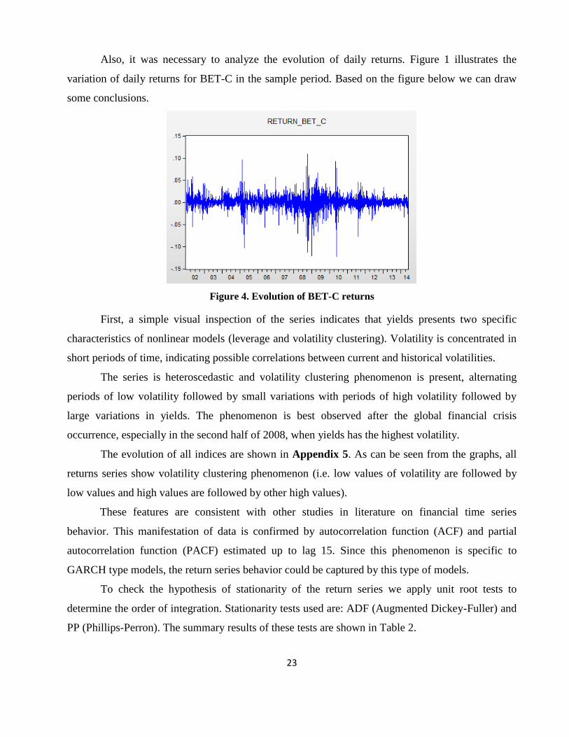
Also, it was necessary to analyze the evolution of daily returns. Figure 1 illustrates the

variation of daily returns for BET-C in the sample period. Based on the figure below we can draw

some conclusions.

Figure 4. Evolution of BET-C returns

First, a simple visual inspection of the series indicates that yields presents two specific

characteristics of nonlinear models (leverage and volatility clustering). Volatility is concentrated in

short periods of time, indicating possible correlations between current and historical volatilities.

The series is heteroscedastic and volatility clustering phenomenon is present, alternating

periods of low volatility followed by small variations with periods of high volatility followed by

large variations in yields. The phenomenon is best observed after the global financial crisis

occurrence, especially in the second half of 2008, when yields has the highest volatility.

The evolution of all indices are shown in Appendix 5. As can be seen from the graphs, all

returns series show volatility clustering phenomenon (i.e. low values of volatility are followed by

low values and high values are followed by other high values).

These features are consistent with other studies in literature on financial time series

behavior. This manifestation of data is confirmed by autocorrelation function (ACF) and partial

autocorrelation function (PACF) estimated up to lag 15. Since this phenomenon is specific to

GARCH type models, the return series behavior could be captured by this type of models.

To check the hypothesis of stationarity of the return series we apply unit root tests to

determine the order of integration. Stationarity tests used are: ADF (Augmented Dickey-Fuller) and

PP (Phillips-Perron). The summary results of these tests are shown in Table 2.

24

Table 2. ADF and PP test results

BET-C BUX DAX FTSE 100 FTSE

MIB

NIKKEI

225 SOFIX S&P 500

ADF test statistic -51.74986 -27.02303 -58.35544 -27.49092 -57.65096 -59.43818 -17.47361 -64.45599

1% -3.432186 -2.565679 -2.565678 -2.565679 -2.565678 -2.565678 -2.565680 -2.565678

5% -2.862237 -1.940922 -1.940922 -1.940922 -1.940922 -1.940922 -1.940922 -1.940922

10% -2.567185 -1.616634 -1.616634 -1.616634 -1.616634 -1.616634 -1.616633 -1.616634

PP test statistic -52.31744 -54.92960 -58.55270 -60.28837 -57.67984 -59.52710 -54.86382 -65.01303

1% -3.432186 -2.565678 -2.565678 -2.565678 -2.565678 -2.565678 -2.565678 -2.565678

5% -2.862237 -1.940922 -1.940922 -1.940922 -1.940922 -1.940922 -1.940922 -1.940922

10% -2.567185 -1.616634 -1.616634 -1.616634 -1.616634 -1.616634 -1.616634 -1.616634

Stationarity tests used have in the null hypothesis that the series analyzed contains a unit

root, i.e. it is not stationary. As can be seen from the table above, for all the series the test statistic

has a value lower than the critical value, at a level of significance of 5% and 1%, and the

probabilities associated are less than 5% (Appendices 6 and 7), which means that the hypothesis of

a unit root is rejected. Therefore return series used in the analyze are stationary. We can say that

they are integrated of order 0.

An important problem posed by financial series is serial correlation of residuals. So we

check if there is correlation in each of the eight rows of data. At first sight, analyzing

autocorrelation functions (ACF) and partial autocorrelation functions (PACF) estimated up to lag 15

it can be seen that there is serial autocorrelation, but this is weak. Autocorrelation and partial

autocorrelation coefficient vary within the range of -0,125 (S&P 500), and 0.107 (SOFIX).

(Appendix 8).

Even if ACF and PACF graphs indicates some autocorrelation, autocorrelation is

insufficiently argued at this point. To confirm the existence of autocorrelation is used Ljung-Box

test. The test confirms the results of visual analysis. Q-test statistic is significantly different from

zero for 6 of the 8 series returns analyzed up to lag 15 and the associated probability is 0% (except

DAX and Nikkei 225), which means that at a level of relevance of 1% we can reject the null

hypothesis of absence of serial correlation.

Autocorrelation analysis should be extended to square returns and absolute returns errors to

check the presence of ARCH effects. Although the autocorrelation function for raw returns indicate

a relatively low correlation, the ACF of square returns indicate significant correlation and

persistence of second order moments. In Annexes 9 and 10 the correlogram of these series are

25

presented. It can be seen that the autocorrelation has increased for all series. In addition, all

autocorrelation coefficients are statistically significant for the first 15 lags and the test null

hypothesis is rejected at a significance level of 1% for all series analyzed, confirming the existence

of serial correlation, so of heteroscedasticity.

There has been increasing evidence of time varying volatility and deviations from normality

in financial time series, and therefore, it is important to conduct a test that is robust to

heteroskedasticity. We perform the variance ratio test of random walk.

An important property of all the random walk hypothesis is that the variance of the residual

variable has to be a linear function of the time.

Considering RW1 = µ + , as returns are independent and follow the same distribution,

we have that Var[ + ] = 2Var[ ]. Therefore, we can determine whether the random walk

hypothesis is plausible by checking variance ratio: VR(2)=

. If RW1 hypothesis is true,

then this report should be significantly equal to one.

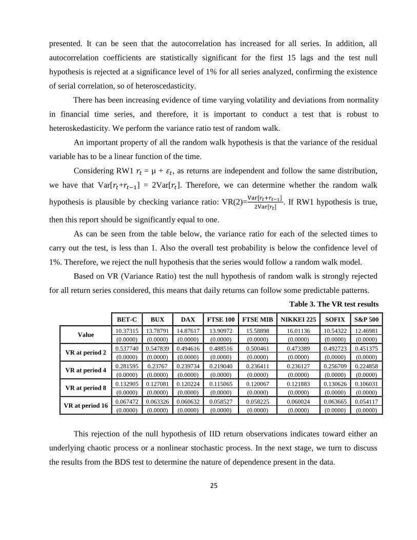
As can be seen from the table below, the variance ratio for each of the selected times to

carry out the test, is less than 1. Also the overall test probability is below the confidence level of

1%. Therefore, we reject the null hypothesis that the series would follow a random walk model.

Based on VR (Variance Ratio) test the null hypothesis of random walk is strongly rejected

for all return series considered, this means that daily returns can follow some predictable patterns.

Table 3. The VR test results

BET-C BUX DAX FTSE 100 FTSE MIB NIKKEI 225 SOFIX S&P 500

Value 10.37315 13.78791 14.87617 13.90972 15.58898 16.01136 10.54322 12.46981

(0.0000) (0.0000) (0.0000) (0.0000) (0.0000) (0.0000) (0.0000) (0.0000)

VR at period 2 0.537740 0.547839 0.494616 0.488516 0.500461 0.473389 0.492723 0.451375

(0.0000) (0.0000) (0.0000) (0.0000) (0.0000) (0.0000) (0.0000) (0.0000)

VR at period 4 0.281595 0.23767 0.239734 0.219040 0.236411 0.236127 0.256709 0.224858

(0.0000) (0.0000) (0.0000) (0.0000) (0.0000) (0.0000) (0.0000) (0.0000)

VR at period 8 0.132905 0.127081 0.120224 0.115065 0.120067 0.121883 0.130626 0.106031

(0.0000) (0.0000) (0.0000) (0.0000) (0.0000) (0.0000) (0.0000) (0.0000)

VR at period 16 0.067472 0.063326 0.060632 0.058527 0.058225 0.060024 0.063665 0.054117

(0.0000) (0.0000) (0.0000) (0.0000) (0.0000) (0.0000) (0.0000) (0.0000)

This rejection of the null hypothesis of IID return observations indicates toward either an

underlying chaotic process or a nonlinear stochastic process. In the next stage, we turn to discuss

the results from the BDS test to determine the nature of dependence present in the data.

26

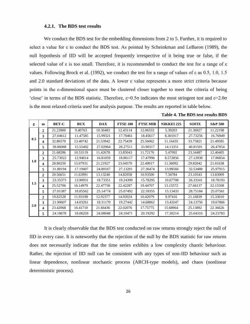
4.2.1. The BDS test results

We conduct the BDS test for the embedding dimensions from 2 to 5. Further, it is required to

select a value for ε to conduct the BDS test. As pointed by Scheinkman and LeBaron (1989), the

null hypothesis of IID will be accepted frequently irrespective of it being true or false, if the

selected value of ε is too small. Therefore, it is recommended to conduct the test for a range of ε

values. Following Brock et al. (1992), we conduct the test for a range of values of ε as 0.5, 1.0, 1.5

and 2.0 standard deviations of the data. A lower ε value represents a more strict criteria because

points in the ε-dimensional space must be clustered closer together to meet the criteria of being

‗close‘ in terms of the BDS statistic. Therefore, ε=0.5σ indicates the most stringent test and ε=2.0σ

is the most relaxed criteria used for analysis purpose. The results are reported in table below.

Table 4. The BDS test results BDS

ε m BET-C BUX DAX FTSE 100 FTSE MIB NIKKEI 225 SOFIX S&P 500

0.5

2 21.23900 9.40763 10.36483 12.43114 12.06333 5.39203 21.36927 11.22198

3 27.04612 11.47585 15.99321 17.70461 18.45617 8.301017 27.73256 16.76949

4 32.86570 13.40742 21.53942 22.75439 25.56062 11.16435 33.75821 21.49585

5 39.86068 15.55492 27.02964 28.27511 33.90317 14.13351 40.81501 26.47854

1.0

2 21.68286 10.53119 11.42678 13.85043 11.72176 5.47092 23.34487 12.40405

3 25.73022 12.94014 16.81059 18.86117 17.47996 8.572856 27.13938 17.86854

4 28.80250 15.07931 21.21927 23.04570 22.49917 11.36092 29.82042 21.81638

5 31.88194 17.19407 24.80167 27.13201 27.36474 13.98566 32.53488 25.97915

1.5

2 20.56651 11.63991 13.13240 14.82958 10.93500 7.34784 23.10543 13.83909

3 23.35373 13.90931 18.73351 19.24399 15.78295 10.67708 26.33341 18.78193

4 25.52706 16.14979 22.47758 22.42287 19.44707 13.15572 27.66137 22.15508

5 27.01387 18.05562 25.14774 25.07492 22.59355 15.13433 28.75184 25.07561

2.0

2 19.82528 11.93198 12.92377 14.92024 10.42079 9.97416 21.16839 15.33010

3 21.90607 14.03261 18.31170 19.27442 14.68862 13.43247 24.13756 19.67866

4 23.42068 16.41710 21.66436 22.02076 17.75775 15.68964 25.13892 22.36626

5 24.18678 18.06259 24.08048 24.10471 20.19292 17.30214 25.64310 24.23783

It is clearly observable that the BDS test conducted on raw returns strongly reject the null of

IID in every case. It is noteworthy that the rejection of the null by the BDS statistic for raw returns

does not necessarily indicate that the time series exhibits a low complexity chaotic behaviour.

Rather, the rejection of IID null can be consistent with any types of non-IID behaviour such as

linear dependence, nonlinear stochastic process (ARCH-type models), and chaos (nonlinear

deterministic process).

27

In the first stage of analysis, we remove the linear dependence in the data by fitting a best

linear model and then conduct the BDS test on linearly filtered residuals to test whether filtered

residuals are IID or not. For this purpose, we estimated through the "least squares method" several

ARMA(m,n) models.

Before estimating this models is necessary to establish the specifications of mean equation.

Based on the autocorrelation coefficients (autocorrelation function) and partial correlation

coefficients (partial autocorrelation function) I have determined the autoregressive starting models.

To choose the right model, namely for the choice of orders m and n, I used the information criterias

Log likelihood, Akaike (Akaike Information Criterion, AIC) and Schwarz (Schwartz Bayesian

Criterion, SBC). These indicators are used when you have to choose an equation from severals.

According to the information criterion is selected the specification for which the log likelihood is

maximum, and AIC and SBC have the lowest values.

ARMA model estimation results are presented in Appendix 12. Considering all the above

mentioned criteria, I considered that best fit models for the daily returns series are: AR(1) – BET-C,

ARMA(2,2) – BUX, ARMA(3,5) – DAX, AR(4)MA(1)MA(3)MA(5) – FTSE 100, ARMA(3,5) –

FTSE MIB, ARMA(3,1) –NIKKEI 225, AR(1)AR(2)MA(2)MA(5) – SOFIX, ARMA(1,8) – S&P

500.

The results of the best fit ARMA models for each series analyzed were summarized in the

table below.

Table 5. Estimated parameters of ARMA models

BET-C BUX DAX FTSE 100

Variable C AR(1) AR(2) MA(2) AR(3) MA(5) AR(4) MA(1) MA(3) MA(5)

Coefficient 0.000526 0.093221 -0.821603 0.759593 -0.041036 -0.052012 0.077791 -0.055223 -0.094939 -0.05658

Std. Error 0.000264 0.017522 0.058591 0.066906 0.017585 0.017585 0.017665 0.017566 0.017521 0.017488

t-Statistic 1.99493 5.3201 -14.02265 11.35309 -2.333569 -2.95775 4.40369 -3.143675 -5.418468 -3.235391

Prob. 0.0461 0.0000 0.0000 0.0000 0.0197 0.0031 0.0000 0.0017 0.0000 0.0012

R-squared 0.008692 0.011914 0.004146 0.019691

Adjusted R-squared 0.008385 0.011608 0.003837 0.018778

S.E. of regression 0.01498 0.015825 0.015339 0.012182

Sum squared resid 0.724383 0.80813 0.759039 0.47833

Log likelihood 8987.145 8807.231 8905.153 9646.933

Mean dependent var 0.000581 0.000296 0.000192 0.0000811

S.D. dependent var 0.015043 0.015918 0.015369 0.012298

Akaike info criterion -5.563557 -5.453844 -5.516204 -5.976407

Schwarz criterion -5.559792 -5.450078 -5.512437 -5.968872

Durbin-Watson stat 2.003313 1.92891 2.052431 1.993533

28

FTSE MIB NIKKEI 225 S&P 500 SOFIX

Variable AR(3) MA(5) AR(3) MA(1) AR(1) MA(8) AR(1) AR(2) MA(2) MA(5)

Coefficient -0.04834 -0.07273 -0.050663 -0.04398 -0.123455 0.040574 0.08823 0.87808 -0.805026 -0.10685

Std. Error 0.017584 0.01757 0.017577 0.017595 0.01747 0.017596 0.012913 0.019701 0.025074 0.015035

t-Statistic -2.74943 -4.13941 -2.88234 -2.49986 -7.066685 2.305947 6.832638 44.56972 -32.10617 -7.10691

Prob. 0.006 0.0000 0.004 0.0125 0.0000 0.0212 0.0000 0.0000 0.0000 0.0000

R-squared 0.007264 0.004585 0.017298 0.045062

Adjusted R-squared 0.006956 0.004277 0.016994 0.044174

S.E. of regression 0.015139 0.015158 0.012664 0.013175

Sum squared resid 0.739396 0.741179 0.517724 0.559829

Log likelihood 8947.47 8943.583 9529.589 9399.9

Mean dependent var -0.000143 0.0000837 0.00015 0.000514

S.D. dependent var 0.015192 0.01519 0.012773 0.013476

Akaike info criterion -5.542423 -5.540014 -5.899436 -5.819696

Schwarz criterion -5.538656 -5.536248 -5.895671 -5.812165

Durbin-Watson stat 2.018552 1.99949 2.007995 1.994088

Since the probabilities attached to t-statistic test are below the 5% level of relevance for both

autoregressive processes AR and moving average MA, the coefficients are considered significant in

statistical terms. Instead, with the exception of the AR (1) for BET-C the constant is not significantly

different from 0. Which is why I reestimated these models without the constant this time.

If the model is well specified, then the residuals from the estimated model are generated by a

white noise process type (sequence of independent random variables, identically distributed) with

zero mean and normally distributed. To detect some dependencies in the residue series ACF and

PACF functions are examined.

In Appendix 14 it can be observed that up to lag 15 autocorrelation and partial correlation

coefficients are not significantly different from 0, which leads to the conclusion that the residues are

not correlated.

The correlogram of squared errors tests the autocorrelation of squared residues of the

regression equation by the same principles as the autocorrelation of the errors. If there is

autocorrelation of squared errors, this is an indication of the existence of heteroscedasticity.

According to the econometric results, for the estimated equations above, in Appendix 15 it can be

observed that there is serial correlation of squared errors, so we may have ARCH terms.

To verify the hypothesis of heteroscedasticity of errors I used the ARCH LM and the White

test.

29

ARCH-LM tests for ARCH effects. The test has the null hypothesis of no ARCH terms.

Since the probabilities attached to F-statistic are in all eight cases below the level of significance of

5%, the null hypothesis is rejected and we accept the presence of these effects.

Table 6. ARCH – LM test results


F-statistic 409.5185 425.4928 114.9481 172.0325 106.49 171.4602 452.5793 127.3903

(0.0000) (0.0000) (0.0000) (0.0000) (0.0000) (0.0000) (0.0000) (0.0000)

Obs*R-

squared

363.6267 376.145 111.0609 163.4191 103.15 162.9055 397.1441 122.6283

(0.0000) (0.0000) (0.0000) (0.0000) (0.0000) (0.0000) (0.0000) (0.0000)

White test relates to the equal spreading of the error in relation to all factors, so that calls to a

regression analysis of the error in relation to the factors. This test has in the null hypothesis that each

coefficient of the regression is significantly different from 0. Since the probability associated with

the test is below the level of significance chosen of 5%, the null hypothesis is rejected. Thus, we

reject the existence of a constant residual variances, so of the homoscedasticity.

Table 7. White test results


F-statistic 221.5869 93.35216 161.9008 97.07056 1413.315 86.84533 107.6564 88.35302

(0.0000) (0.0000) (0.0000) (0.0000) (0.0000) (0.0000) (0.0000) (0.0000)

Obs*R-

squared

390.0228 257.9994 422.6342 748.1937 748.1937 241.355 809.4476 245.2381

(0.0000) (0.0000) (0.0000) (0.0000) (0.0000) (0.0000) (0.0000) (0.0000)

Scaled

explained SS

2324.938 1017.242 1429.228 3188.237 3188.237 981.9791 3729.383 1343.214

(0.0000) (0.0000) (0.0000) (0.0000) (0.0000) (0.0000) (0.0000) (0.0000)

The lack of serial correlation shown by the correlogram of errors is confirmed by the test

Serial Correlation LM test. The null hypothesis of the test is that there is no serial correlation of the

errors of the regression equation. The probability associated with the test is greater than 0.05 (except

BUX and FTSE 100), it is higher than the level of relevance. The null hypothesis is accepted, so we

accept the absence of serial correlation.

Table 8. BG test results


F-statistic 1.089652 4.06943 2.219754 4.986172 0.287987 0.218754 0.056391 3.454432

(0.2966) (0.0437) (0.1364) (0.0256) (0.5916) (0.6400) (0.8123) (0.0632)

Obs*R-

squared

1.090297 2.833148 1.611008 4.79288 0.00000 0.099708 0.00000 2.923412

(0.2964) (0.0923) (0.2044) (0.0286) (1.00000) (0.7522) (1.00000) (0.0873)

30

To test the normality of errors it is used Jarque-Bera test. The normal distribution of errors is

especially important when we want to make predictions based on the econometric equation

estimated. Since the probability associated Jarque-Bera test is 0%, we can say that the errors of

ARMA models are not normally distributed.

Table 9. Descriptive statistics for ARMA models


Medie -7.36E-19 0.00031 0.000211 0.0000943 -0.000161 0.0000921 0.000209 0.000162

Mediană 0.0000456 0.000464 0.000769 0.000475 0.000633 0.000403 0.000213 0.000842

Maxim 0.10125 0.119075 0.1058 0.085409 0.106367 0.09478 0.08635 0.108108

Minim -0.12488 -0.118569 -0.075804 -0.086543 -0.089539 -0.118087 -0.090797 -0.094631

Deviaţia standard 0.014978 0.015819 0.015335 0.012176 0.015136 0.015155 0.013168 0.012661

Skewness -0.574155 -0.115486 -0.021898 -0.318741 -0.139341 -0.693595 -0.050305 -0.290047

Kurtotica 12.93684 8.908951 7.774825 9.554318 7.658367 9.164627 10.24436 11.98577

Jarque-Bera 13466.33 4704.79 3066.717 5830.849 2929.147 5370.171 7062.21 10912.1

Probabilitate 0.000000 0.000000 0.000000 0.000000 0.000000 0.000000 0.000000 0.000000

We now conduct the BDS test on ARMA residuals. The results are reported in Table 10.

Again it is clearly observable that the the null of IID is strongly reject in every case. The rejection of

null hypothesis at this stage suggests that some kind of dependence is still left in the data. Since

linear structures have already been removed using the best fit autoregressive–moving-average

model, the rejection of null hypothesis is indicative of some nonlinear dependencies in the returns

series.

Table 10. BDS test results


0.5

2 20.85404 9.05669 10.72699 11.98833 11.62502 4.61095 20.48468 9.84113

3 26.73114 11.21028 16.43940 17.82753 18.27849 7.55941 27.32732 15.59580

4 32.44339 12.96338 22.12497 23.45954 25.71516 10.62564 33.83649 20.31128

5 39.48533 14.87797 27.80116 29.76924 34.38904 14.46141 41.82862 25.05381

1.0

2 21.47715 10.06301 11.47863 13.42828 11.48518 4.76526 22.78616 11.28315

3 25.78233 12.30262 16.97194 18.67017 17.27493 7.89080 27.29603 16.99293

4 28.89316 14.33610 21.43380 23.18735 22.40226 10.68752 30.39679 21.01966

5 32.08189 16.29264 25.07085 27.62683 27.29821 13.32575 33.44802 25.13252

1.5

2 20.85124 11.21513 12.99526 14.07523 10.99497 6.67766 23.04555 13.31352

3 24.05517 13.07780 18.68524 18.78007 15.78002 9.84248 26.64263 18.31499

4 26.23713 15.19643 22.43234 22.24422 19.50648 12.32883 28.19900 21.70267

5 27.82834 16.98912 25.12748 25.13560 22.66971 14.32270 29.57038 24.69741

2.0

2 20.07422 11.78482 12.94515 14.34879 10.52895 9.32508 22.26887 14.63865

3 22.67976 13.40236 18.30898 19.00731 14.69481 12.62530 25.24498 19.07058

4 24.20914 15.67073 21.67818 22.01718 17.77636 14.88138 26.16900 21.78561

5 25.01601 17.17728 24.11509 24.21664 20.24158 16.50055 26.72446 23.74991

31

After the confirmation that some type of nonlinearity is present in the data, we next move to

investigate the nature of this nonlinearity, i.e. stochastic or deterministic, by using the BDS test of

independence. We conduct the BDS test on the data after removing the nonlinear dependence

caused by heteroskedasticity. We use different ARCH type models for daily returns series.

In this step we will try to trace the equation that best describes the volatility of daily returns

series. Before estimating a GARCH model we have selected the best ARMA models for the return

series analyzed and shown that they have significant statistic coefficients. According to the Jarque-

Bera test the error distribution is not normal. White test for heteroscedasticity confirmed the

presence of ARCH effects. And with ACF and PACF functions we analyzed the autocorrelation and

we concluded that residues are not correlated, but instead we have significant serial correlation of

squared errors. Therefore a GARCH type model may be considered an appropriate change to the

initial model.

For the choice of orders p and q, and the type of ARCH model (GARCH / TGARCH,

GARCH-M, EGARCH, PARCH) were made successive attempts to find the desired equation and

were analyzed all possible combinations seeking to maximize criterion Log likelihood, and AIC and

SBC criteria minimization.

I also compared the results obtained for the three possible distributions: normal distribution,

Student-t and GED ("Generalized Error Distribution").

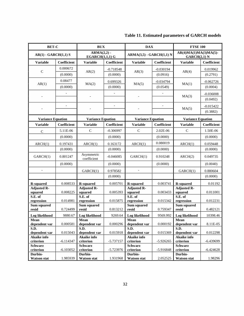
After this comparison between GARCH models for volatility modeling, we decided to fit the

data with the following models: BET-C – GARCH(1,1), BUX – EGARCH(1,1,1), DAX –

GARCH(1,1), FTSE 100 – GARCH(2,1), FTSE MIB – GARCH(1,1), NIKKEI – GARCH(1,1),

SOFIX – EGARCH(1,1,1), S&P 500– EGARCH(2,1,1).

The results of the best fit GARCH models for each series analyzed were summarized in table

11 below.

Square error and conditional variance coefficients of the variance equation are statistically

significant (significance level of 1% and 5%).

32

Table 11. Estimated parameters of GARCH models

BET-C BUX DAX FTSE 100

AR(1) - GARCH(1,1) S ARMA(2,2) -

EGARCH(1,1,1) G ARMA(3,5) - GARCH(1,1) N

AR(4)MA(1)MA(3)MA(5)-

GARCH(2,1) N

Variable Coefficient Variable Coefficient Variable Coefficient Variable Coefficient

C 0.000672

AR(2) -0.718548

AR(3) -0.030194

AR(4) 0.019962

(0.0000) (0.0000) (0.0916) (0.2791)

AR(1) 0.08477

MA(2) 0.699326

MA(5) -0.034794

MA(1) -0.062726

(0.0000) (0.0000) (0.0549) (0.0004)

- -

- -

- -

MA(3) -0.036008

(0.0492)

- -

- -

- -

MA(5) -0.015422

(0.3882)

Variance Equation Variance Equation Variance Equation Variance Equation


C 5.11E-06 C -0.306997 C 2.02E-06 C 1.50E-06

(0.0000) (0.0000) (0.0000) (0.0000)

ARCH(1) 0.197431 ARCH(1) 0.163172 ARCH(1) 0.080019 ARCH(1) 0.059448

(0.0000) (0.0000) (0.0000) (0.0000)

GARCH(1) 0.801247 Asymmetric

coefficient -0.046085 GARCH(1) 0.910248 ARCH(2) 0.049735

(0.0000) (0.0000) (0.0000) (0.0040)

- GARCH(1) 0.978582 - GARCH(1) 0.880604

(0.0000) (0.0000)

R-squared 0.008533 R-squared 0.005701 R-squared 0.003741 R-squared 0.01192

Adjusted R-

squared 0.008225 Adjusted R-



squared 0.011001

S.E. of

regression 0.014981 S.E. of



regression 0.012231

Sum squared

resid 0.724499 Sum squared



resid 0.482121

Log likelihood 9880.67 Log likelihood 9269.64 Log likelihood 9569.992 Log likelihood 10398.46

Mean

dependent var 0.000581 Mean



dependent var 8.11E-05

S.D.

dependent var 0.015043 S.D.



dependent var 0.012298

Akaike info

criterion -6.114347 Akaike info



criterion -6.439699

Schwarz

criterion -6.103052 Schwarz



criterion -6.424628

Durbin-

Watson stat 1.985939 Durbin-



Watson stat 1.98296

33

FTSE MIB NIKKEI 225 S&P 500 SOFIX

ARMA(3,5)-GARCH(1,1) N ARMA(3,1)-GARCH(1,1) N ARMA(1,8)-

EGARCH(2,1,1) G

AR(1)AR(2)MA(2)MA(5)-

EGARCH(1,1,1) G


C -0.026186

AR(3) 0.00917

AR(1) -0.076468

AR(1) 0.060901

(0.1430) (0.5906) (0.0000) (0.0000)

AR(1) -0.029998

MA(1) -0.035908

MA(8) 0.009361

AR(2) 0.840472

(0.0886) (0.0781) (0.5731) (0.0000)

- -

- -

- -

MA(2) -0.810569

(0.0000)

- -

- -

- -

MA(5) -0.024328

(0.0417)

Variance Equation Variance Equation Variance Equation Variance Equation


C 9.82E-07 C 3.41E-06 C -2.94E-01 C -0.943369

(0.0000) (0.0000) (0.0000) (0.0000)

ARCH(1) 0.074271 ARCH(1) 0.09109 ARCH(1) -0.125145 ARCH(1) 0.464986

(0.0000) (0.0000) (0.0052) (0.0000)

GARCH(1) 0.923379 GARCH(1) 0.895046 ARCH(2) 0.252789 Asymmetric

coefficient -0.044994

(0.0000) (0.0000) (0.0000) (0.0308)

-

-

Asymmetric

coefficient -0.139159 GARCH(1) 0.933315

(0.0000) (0.0000)

- - GARCH(1) 0.978603 -

(0.0000)

R-squared 0.005046 R-squared 0.000923 R-squared 0.013929 R-squared 0.029677

Adjusted R-




squared 0.028774

S.E. of




regression 0.013281

Sum squared




resid 0.568849

Log likelihood 9598.664 Log likelihood 9361.708 Log likelihood 10497.75 Log likelihood 10378.38

Mean

dependent var -0.000143 Mean

dependent var 8.37E-05 Mean



S.D.





Akaike info

criterion -5.94403

Akaike info

criterion -5.797217

Akaike info

criterion -6.495199

Akaike info

criterion -6.422657

Schwarz




criterion -6.405711

Durbin-




Watson stat 1.95012

34

In EGARCH models for BUX, S&P 500 and SOFIX the asymmetric coefficient seems to be

statistically significant because the probabilities attached are less than 5%. To confirm this, we

applied the Wald test. This test has the null hypothesis that these coefficients are not significantly

different from zero.

Table 12. The Wald test results

t-statistic F-statistic Chi-square

BUX -4.73663

(0.0000)

22.43568

(0.0000)

22.43568

(0.0000)

S&P 500 -12.0982

(0.0000)

146.3661

(0.0000)

146.3661

(0.0000)

SOFIX -2.16009

(0.0308)

4.665999

(0.0308)

4.665999

(0.0308)

Since in all three cases the probabilities attached are less than the critical value of 0.05, the

null hypothesis of the test is rejected, which means that in these cases the impact of the information

will be asymmetrical.

As expected, when estimating a GARCH model for financial data series, the sum of

coefficients is very close to 1. The constant term is very small, and the conditional variance

coefficient is greater than 0.8 in all cases, this means that shocks in the conditional variance are

persistent and significant changes in the conditional variance are followed by other large changes,

and small changes by other small changes.

Having established suitable models for the return series considered, now they must be

assessed by a number of statistical tests and graphs. If the models are correctly specified, then the

standardized residues must not longer poses serial correlation, heteroscedasticity or any other type

of non-linear dependence.

Therefore, for the beginning we estimate the ACF and PACF functions of the squared

standardized residuals of the models and use Q-statistics (Ljung-Box) test to investigate the

existence of serial correlation up to lag 15.

According to correlogram of squared errors (shown in Appendix 22), there is no additional

ARCH terms. Since the coefficients of autocorrelation and partial correlation functions are very

close to the value 0 it can be stated that residues are not correlated.

35

Also, the probability of more than 5% of the Q-statistic test, corresponding to the null

hypothesis that there is no autocorrelation in residues up to lag 15, confirms the absence of

autocorrelation for the squared errors.

Further, the existence of other possible ARCH effects remaining in the residue is tested

using ARCH-LM test. If the variance equation proposed by our model is correctly specified, then

we should not have more ARCH effects.

LM test investigates the null hypothesis of absence of ARCH effects and it is necessary to

have an estimated value that is not statistically significant to not have the power to reject H0.

Table 13. The ARCH – LM test results


F-statistic 3.241016 0.589139 2.972783 0.497674 2.118539 1.026956 0.062340 0.080758

(0.0719) (0.4428) (0.0848) (0.4806) (0.1456) (0.3110) (0.8029) (0.7763)

Obs*R-

squared

3.239771 0.589397 2.971887 0.497906 2.118461 1.027265 0.062378 0.080806

(0.0719) (0.4428) (0.0847) (0.4804) (0.1455) (0.3108) (0.8028) (0.7762)

ARCH LM test shows that we can accept the null hypothesis of absence of ARCH effects as

attached test probabilities are greater than 0.05, the results not having statistical significance.

Jarque-Bera test also confirms that the residues are still not normally distributed.(Prob = 0%)

Table 14. Descriptive statistics for GARCH models


Medie 0.000933 0.029533 0.024918 0.011698 -0.006387 0.006999 0.038238 0.018818

Mediană -0.011723 0.032606 0.063245 0.037652 0.044786 0.023157 0.027858 0.091280

Maxim 7.949975 4.112991 3.395123 4.434716 4.680145 3.267584 6.566573 3.625933

Minim -6.844023 -5.369757 -6.817613 -4.407328 -5.169177 -5.404181 -5.900159 -6.482276

Deviaţia standard 0.992793 1.000605 1.000360 1.000246 1.000198 1.000147 1.006995 1.000690

Skewness 0.128544 -0.064769 -0.353129 -0.309079 -0.378137 -0.383344 0.192677 -0.450817

Kurtotica 7.142378 4.010356 4.251021 3.708267 4.230684 4.024651 6.642557 4.210318

Jarque-Bera 2318.25 139.6003 277.5886 118.8290 280.6386 220.2734 1805.108 306.5558

Probabilitate 0.000000 0.000000 0.000000 0.000000 0.000000 0.000000 0.000000 0.000000

We now apply the BDS test of independence to standardized residuals of GARCH and

EGARCH models. In doing so, we use the BDS test to test the null hypothesis of independent

random variables against the alternative hypothesis of non-independent random variables. The

results are presented in Table 15.

36

The results suggest that the ARCH-type models have removed considerable serial

dependence from the raw and filtered data and also the values of BDS statistic are noticeably

reduced at all dimensions. It is also observable that the null hypothesis is not rejected in six cases,

i.e. BUX, DAX, FTSE 100, FTSE MIB, NIKKEI 225 and S&P 500.

The non-rejection of the null hypothesis at this stage of the analysis indicates that

conditional heteroskedasticity is the main cause for the initial rejection of the null and the nature of

dependence in the data is best described as a nonlinear stochastic system. It appears, therefore, that

the behaviour of these return series is adequately explained by ARCH-type models. However, the

null hypothesis is again rejected for BET-C and SOFIX. In these cases, the significant BDS

statistics for the standardized residuals suggest that the returns series are non-IID and the ARCH

type models are not sufficient to capture all the information present in the data. The rejection of the

null hypothesis, at this stage, is consistent with deterministic chaos as there remains some further

dependence in the data that cannot be explained with reference to GARCH and EGARCH models.

Table 15. The BDS test results


0.5

2 4.825549 -0.081942* -1.653390* -0.881034* -1.682837* -2.423919 3.913801 -1.033641*

3 5.305013 -0.377128* -0.024019* 0.338339* -1.001259* -1.717043* 4.460895 -0.425269*

4 5.492119 -0.378757* 1.452941* 1.055317* 0.023915* -0.641525* 4.013648 -0.352227*

5 5.172980 0.000480* 2.482784 1.668677* 0.570817* 0.234327* 3.452289 -0.266141*

1.0

2 3.985862 -0.694551* -2.645580 -0.650178* -1.990842 -3.992148 3.175269 -0.975392*

3 3.690628 -1.081481* -1.296131* 0.146274* -1.241394* -3.532882 3.509793 -0.858417*

4 3.367446 -1.057247* -0.017167* 0.718921* -0.184242* -2.591520 3.280873 -0.852200*

5 2.705422 -0.813497* 0.790931* 1.165214* 0.442030* -1.823461* 2.660342 -0.773877*

1.5

2 3.584677 -0.542837* -2.968780 -0.295083* -2.372692 -4.056215 2.300337 -0.577788*

3 3.188778 -0.86931* -1.969512 0.099768* -1.953353* -3.464264 2.610313 -0.547093*

4 2.845470 -0.708258* -0.883220* 0.393346* -0.956526* -2.786503 2.561622 -0.670607*

5 2.221953 -0.459095* -0.267057* 0.708122* -0.372994* -2.218547 2.157721 -0.676532*

2.0

2 3.212322 -0.056239* -2.641131 0.531851* -2.178616 -3.290453 1.364244* -0.275873*

3 2.806847 -0.180037* -1.630612* 0.539393* -1.953942* -2.700124 1.510578* -0.282918*

4 2.498565 0.144142* -0.681718* 0.588599* -1.092264* -2.147277 1.644802* -0.558696*

5 1.958490* 0.394994* -0.193644* 0.794627* -0.529896* -1.749933* 1.394414* -0.662614*

(*) Indicates BDS statistics that are not significant at 5% critical level

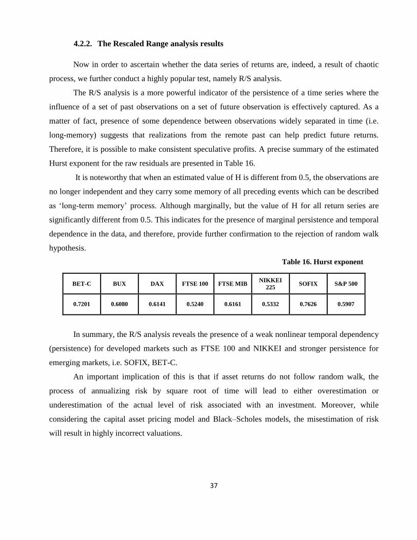
37

4.2.2. The Rescaled Range analysis results

Now in order to ascertain whether the data series of returns are, indeed, a result of chaotic

process, we further conduct a highly popular test, namely R/S analysis.

The R/S analysis is a more powerful indicator of the persistence of a time series where the

influence of a set of past observations on a set of future observation is effectively captured. As a

matter of fact, presence of some dependence between observations widely separated in time (i.e.

long-memory) suggests that realizations from the remote past can help predict future returns.

Therefore, it is possible to make consistent speculative profits. A precise summary of the estimated

Hurst exponent for the raw residuals are presented in Table 16.

It is noteworthy that when an estimated value of H is different from 0.5, the observations are

no longer independent and they carry some memory of all preceding events which can be described

as ‗long-term memory‘ process. Although marginally, but the value of H for all return series are

significantly different from 0.5. This indicates for the presence of marginal persistence and temporal

dependence in the data, and therefore, provide further confirmation to the rejection of random walk

hypothesis.

Table 16. Hurst exponent

BET-C BUX DAX FTSE 100 FTSE MIB NIKKEI

225 SOFIX S&P 500

0.7201 0.6080 0.6141 0.5240 0.6161 0.5332 0.7626 0.5907

In summary, the R/S analysis reveals the presence of a weak nonlinear temporal dependency

(persistence) for developed markets such as FTSE 100 and NIKKEI and stronger persistence for

emerging markets, i.e. SOFIX, BET-C.

An important implication of this is that if asset returns do not follow random walk, the

process of annualizing risk by square root of time will lead to either overestimation or

underestimation of the actual level of risk associated with an investment. Moreover, while

considering the capital asset pricing model and Black–Scholes models, the misestimation of risk

will result in highly incorrect valuations.

38

4.2.3. The Rcurrence Analysis results

The eight series data of indices were analysed with Visual Recurrence Analysis. The data

were implemented and analysed without prewhitening.

The Recurrence Plots are shown below. There were built using a delay-time equal to 1 and

embedding dimension determined by the method of false nearest neighbours.

Figure 5. RP – DAX Figure 6. RP – FTSE 100 Figure 7. RP – S&P 500

Figures 5, 6 and 7 represent distance plots for the three largest Western financial markets:

Germany, the United Kingdom and the United States. These plots exhibit many common features,

possibly reflecting the high level of integration of these markets. Light shaded regions are always

found in the vicinity of the main diagonal line. The light shading fades as the distance to the LoI

increases, reflecting the non-stationarity of the series. However, interesting light shaded structures

can be found far from the LoI. A ‗‗butterfly‘‘ shaped structure can be observed in the three plots.

Figure 8. RP – BET-C Figure 9. RP – FTSE MIB Figure 10. RP – BUX

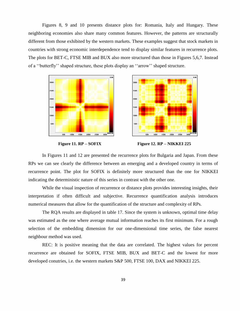
39

Figures 8, 9 and 10 presents distance plots for: Romania, Italy and Hungary. These

neighboring economies also share many common features. However, the patterns are structurally

different from those exhibited by the western markets. These examples suggest that stock markets in

countries with strong economic interdependence tend to display similar features in recurrence plots.

The plots for BET-C, FTSE MIB and BUX also more structured than those in Figures 5,6,7. Instead

of a ‗‗butterfly‘‘ shaped structure, these plots display an ‗‗arrow‘‘ shaped structure.

Figure 11. RP – SOFIX Figure 12. RP – NIKKEI 225

In Figures 11 and 12 are presented the recurrence plots for Bulgaria and Japan. From these

RPs we can see clearly the difference between an emerging and a developed country in terms of

recurrence point. The plot for SOFIX is definitely more structured than the one for NIKKEI

indicating the deterministic nature of this series in contrast with the other one.

While the visual inspection of recurrence or distance plots provides interesting insights, their

interpretation if often difficult and subjective. Recurrence quantification analysis introduces

numerical measures that allow for the quantification of the structure and complexity of RPs.

The RQA results are displayed in table 17. Since the system is unknown, optimal time delay

was estimated as the one where average mutual information reaches its first minimum. For a rough

selection of the embedding dimension for our one-dimensional time series, the false nearest

neighbour method was used.

REC: It is positive meaning that the data are correlated. The highest values for percent

recurrence are obtained for SOFIX, FTSE MIB, BUX and BET-C and the lowest for more

developed conutries, i.e. the western markets S&P 500, FTSE 100, DAX and NIKKEI 225.

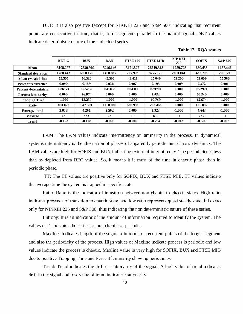
40

DET: It is also positive (except for NIKKEI 225 and S&P 500) indicating that recurrent

points are consecutive in time, that is, form segments parallel to the main diagonal. DET values

indicate deterministic nature of the embedded series.

Table 17. RQA results

LAM: The LAM values indicate intermittency or laminarity in the process. In dynamical

systems intermittency is the alternation of phases of apparently periodic and chaotic dynamics. The

LAM values are high for SOFIX and BUX indicating extent of intermittency. The periodicity is less

than as depicted from REC values. So, it means it is most of the time in chaotic phase than in

periodic phase.

TT: The TT values are positive only for SOFIX, BUX and FTSE MIB. TT values indicate

the average time the system is trapped in specific state.

Ratio: Ratio is the indicator of transition between non chaotic to chaotic states. High ratio

indicates presence of transition to chaotic state, and low ratio represents quasi steady state. It is zero

only for NIKKEI 225 and S&P 500, thus indicating the non deterministic nature of these series.

Entropy: It is an indicator of the amount of information required to identify the system. The

values of -1 indicates the series are non chaotic or periodic.

Maxline: Indicates length of the segment in terms of recurrent points of the longer segment

and also the periodicity of the process. High values of Maxline indicate process is periodic and low

values indicate the process is chaotic. Maxline value is very high for SOFIX, BUX and FTSE MIB

due to positive Trapping Time and Percent laminarity showing periodicity.

Trend: Trend indicates the drift or stationarity of the signal. A high value of trend indicates

drift in the signal and low value of trend indicates stationarity.

BET-C BUX DAX FTSE 100 FTSE MIB NIKKEI

225 SOFIX S&P 500

Mean 3108.297 17530.949 5246.146 5171.527 26219.318 11759.728 660.458 1157.442

Standard deviation 1788.443 6000.125 1400.887 797.902 8275.176 2860.041 432.708 200.121

Mean rescaled dist 53.567 36.323 43.390 49.421 35.049 52.293 52.699 55.588

Percent recurrence 0.090 0.159 0.036 0.007 0.195 0.009 0.372 0.001

Percent determinism 0.36174 0.55257 0.41858 0.04310 0.39701 0.000 0.72921 0.000

Percent laminarity 0.000 26.974 0.000 0.000 3.032 0.000 50.340 0.000

Trapping Time -1.000 13.259 -1.000 -1.000 10.769 -1.000 12.674 -1.000

Ratio 400.878 347.301 1158.080 620.988 203.468 0.000 195.807 0.000

Entropy (bits) 3.038 4.261 2.502 0.000 3.923 -1.000 4.643 -1.000

Maxline 25 562 45 10 600 -1 762 -1

Trend -0.153 -0.198 -0.056 -0.010 -0.234 -0.013 -0.566 -0.002

41

The analysis led with VRA induces us to refuse the hypothesis of IID and to emphasize the

presence of structure. The data are non-linear deterministic in six out of eight cases and this

nonlinearity can be interpreted as chaos. The most evident results are obtained for the emerging

countries.

Predicting with VRA

Even if we are not interested in time series forecasting as a subject matter, we can think of it

as the ultimate test of your analysis of a particular dynamical system and the time series generated

by that system. If our embedding parameters are optimal, than the corresponding predictive model

should minimizes the prediction error.

VRA provides an important module on non-parametric forecasting, using local models by

fitting a low order polynomial which maps k nearest neighbours of onto their next values, to use this

map to predict future values.After prediction, a plot shows the actual and predicted values, jointly

with the normalized prediction error and the magnitudes of RMSE (root of the mean squared error)

and normalized error (mean squared error normalized by the mean squared error of the trivial

predictor: the unconditional mean in multi-step forecasting, or the random walk predictor in the one-

step ahead predictor). In Appendix 14 are presented in sample predictions for all series analyzed.

From Figures 13 and 14 once again we can notice the difference between an emerging and a

developed country in terms of in sample prediction. The RMSE is very low for SOFIX ( i.e. 5.24),

while for NIKKEI 225 is 514.40, a very high value. This suggests that in a country with well

developed financial market it is not easy to make predictions. Intertemporal smoothing operations,

such as arbitrage, tend to squash cycles and chaos in economic systems with rich enough variety of

market instruments. However, given the very different institutional features of financial markets in

developing countries, it is important to explore the possibilities of such markets exhibiting chaotic

behavior. Financial markets in developing countries are less mature as compared to those in

developed countries, and the implications of complex nonlinear behavior could be significant for

traders, institutional investors for devising suitable trading strategies.

Common fallacies about markets claim financial markets are unpredictable. However, chaos

theory together with powerful algorithms proves such statements are wrong. Markets are chaotic

systems with complex dynamics, yet to a certain extent we can make valid stock market forecasts.

Using these forecasts together with a careful risk management strategy may give a trader a

significant competitive advantage.

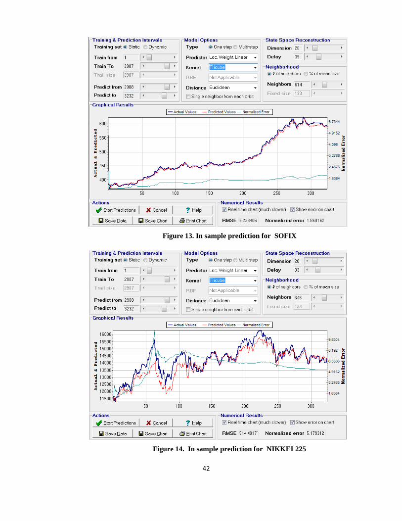
42

Figure 13. In sample prediction for SOFIX

Figure 14. In sample prediction for NIKKEI 225

43

CONCLUSIONS

This study has examined the time series behaviour of close price based daily returns of

equity indices for different markets by using recently developed tests of independence, nonlinearity

and chaos.

Sometimes the conclusions both for and against chaos are reached by applying only one type

of chaos test. To produce convincing results, we have to employ all tests for chaos to exploit their

different potentials and limits. Few published papers have jointly applied the BDS test, R/S analysis,

and topological tests.

Until recently, financial market researchers were ill equipped to detect the presence of chaos.

The most commonly used nonlinear testing procedure was the BDS test, which is poorly suited for

application to the small, noisy data sets common in finance. The introduction of recurrence plots

and RQA for chaotic behaviour, however, has provided researchers with an exciting new tool for

detecting chaos in financial data.

There are few existing studies of complex nonlinear dynamics which utilize this

methodology, and so the application in this paper serves to illustrate the potential of this tool in the

study of financial data, but more important to support the conclusion that the data analysed could be

chaotic

In short, consistent with the findings of many previous studies results of this study reveal

that there is a strong evidence of nonlinear dependence in daily increments of all equity indices

analyzed. However, the nature of this nonlinear dependence appears to be deterministic only in five

out of six cases.

More precisely, the results of variance ratio test suggest that the null hypothesis of random

walk is strongly rejected for all the return series. It appears that daily increment in stock returns are

highly autocorrelated. Further, the results based on Rescaled Range analysis also reveal that there is

evidence of persistence or temporal dependencies in daily increments of market returns. The BDS

test of independence produced mixed results when conducted on standardized residuals from

GARCH and EGARCH models. In six out of eight cases the null of IID was not rejected. Non-

rejection of the null hypothesis of IID observations suggests that low order GARCH or EGARCH

type models are adequate to capture all potential nonlinear dependence in the data.

44

The findings of this study have some interesting implications. First, the existence of chaos in

market indices could be exploitable and helpful for market players in the emerging countries such as

Romania and Bulgaria. In other words, the presence of chaotic structure in return series implies that

profitable nonlinearity based trading rules may exist at least in the short-run.

Second, presence of nonlinearity in the data suggests that asset pricing models and

forecasting models should account for the existing nonlinearities in the data, otherwise their results

may be biased and highly misleading. Finally, the presence of temporal dependence in market

returns, as confirmed by the estimates of Hurst exponent, suggests that the process of annualizing

risk by square root of time may lead to either overestimation or underestimation of the actual level

of risk associated with an investment.

The VRA analysis, which can be applied and gives reliable results also with short data sets,

shows presence of chaotic behaviour in five out of eight cases.

There are important reasons to understand the impact of nonlinearities and chaos in financial

markets. Even if the future is unknowable, nonetheless Chaos Theory allows for the possibility of a

range of future states represented by attractor on which orbits chaotic trajectories evolve. In the long

run, a chaotic system moves into, and remains in it, though in principle determinate, resembles a

random walk, repeatedly visiting each point in the attractor. The global behaviour of chaotic

systems is bounded on the attractor: is not explosive. While economic fluctuations are unpredictable

they will always lie within certain bounds. Thus, if we are able to know in which space the attractor

lies, by determining the phase space using the embedding dimension for instance, and if we are able

to re-build the orbits, then we can make predictions.

Although we cannot forecast the precise state of a chaotic system in the longer term, chaotic

systems trace repetitive patterns which often provide useful information because they are the same

at different scale of time. What is observed at a more global level is reproduced at a smaller scale

because the chaotic attractor is a fractal. So, having knowledge of such patterns would make it

possible to, on the average, make better predictions in short term.

45

REFERENCES

1. Barkoulas, J. T. (2008), ―Testing for Deterministic Monetary Chaos: Metric and Topological

Diagnostics‖, Chaos, Solitons and Fractals, 38, 1013–1024;

2. Bastos, A. J. and J. Caiado (2010), ―Recurrence Quantification Analysis of Global Stock

Markets‖;

3. Bhattacharya, A. and R. Sensarma (2006), ―Do Financial Markets Exhibit Chaotic Behaviour?

Evidence from an Emerging Economy‖;

4. Crowley, P. and A. Schultz (2010), ―A New Approach to Analyzing Convergence and

Synchronicity in Growth and Business Cycles: Cross Recurrence Plots and Quantification

Analysis‖;

5. Dechert, D. W. and C. H. Hommes (2000), ―Complex Nonlinear Dynamics and Computational

Methods‖, Journal of Economic Dynamics and Control, 24, 651-662;

6. Diebolt, C. and C. Kyrtsou (2005), ―New Trends in Macroeconomics‖;

7. Eckmann, J. P., S. O. Kamphorst, and D. Ruelle (1987), ―Recurrence Plots of Dynamical

Systems‖, Europhys. Lett., 4 (9), 973-977;

8. Faggini, M. (2013), ―Chaos Detection in Economic Time Series: Metric versus Topological

Tools‖;

9. Faggini, M. and A. Parziale (2011), ―The Failure of Economic Theory. Lessons from Chaos

Theory‖;

10. Farmer, D. J. (1981), ―Chaotic Attractors of an Infinite-Dimensional Dynamical System‖ ;

11. Guégan, D. (2009), ―Chaos in Economics and Finance‖;

12. Karytinos, A. D. (1999), ―A Chaos Theory and Nonlinear Dynamics Approach to the Analysis

of Financial Series: A Comparative Study of Athens and London Stock Markets‖, A

Dissertation Presented for the Doctor of Philosophy Degree;

46

13. Kemp, E. S. (2006), ―Gamma Test Analysis Tools for Non-linear Time Series‖;

14. Kennel, M. B., R. Brown, and H. D. I. Abarbanel, (1992), ―Determining Embedding

Dimension for Phase-Space Reconstruction Using a Geometrical Construction‖, Physical

Review A, Vol. 45, No. 6;

15. LeBaron, B. (1994), ―Chaos and Nonlinear Forecastability in Economics and Finance‖,

University of Wisconsin – Madison;

16. Marwan, N. and J. Kurths (2005), ―Line Structures In Recurrence Plots‖, Physics Letters A, 336,

349–357;

17. Marwan, N., M. C. Romano, M. Thiel, and J. Kurths (2007), ―Recurrence Plots for the Analysis

of Complex Systems‖, Physics Reports, 438, 237 – 329;

18. McKenzie, D. M. (2001), ―Chaotic Behavior in National Stock Market Indices: New Evidence

from the Close Returns Test‖, Global Finance Journal, 12, 35-53;

19. Mhalsekar, S. D., S. S. Rao, and K.V. Gangadharan (2010), ―Investigation on Feasibility of

Recurrence Quantification Analysis for Detecting Flank Wear in face Milling‖, International

Journal of Engineering, Science and Technology, Vol. 2, No. 5, 23-38;

20. Mirowski, P., ―From Mandelbrot to Chaos in Economic Theory‖, 289-307, University of Notre

Dame, Notre Dame, Indiana;

21. Mishra, R. K., S. Sehgal, and N. R. Bhanumurthy (2011), ―A Search for Long-Range

Dependence and Chaotic Structure in Indian Stock Market‖, Review of Financial Economics,

20, 96-104;

22. Moloney, K. and S. Raghavendra, ―Transition Dynamics of Dow Jones Index Using Recurrence

Quantification Analysis : From Bull to Bear‖;

23. Özer, G. and C. Ertokatli (2010), ―Chaotic Processes of Common Stock Index Returns: An

Empirical Examination on Istanbul Stock Exchange (ISE) Market‖;

24. Peters, E. E. (1991), ―Chaos and Order in the Capital Markets: A New View of Cycles, Prices,

and Market Volatility‖;

47

25. Pincus, M. S. (1990), ―Approximate Entropy as a Measure of System Complexity‖;

26. Schultz, A. P., Y. Zou, N. Marwan, and M. T. Turvey (2011), ―Local Minima-Based Recurrence

Plots for Continuous Dynamical Systems‖, International Journal of Bifurcation and Chaos, Vol.

21, No. 4, 1065-1075;

27. Yamaguchi, K. (2014), ―Money and Macroeconomic Dynamics: Accounting System Dynamics

Approach‖ ;

28. Zbilut, J. P., A. Giuliani, and C. L. Webber (2008), ―Recurrence Quantification Analysis and

Principal Components in the Detection of Short Complex Signals‖;

29. Zbilut, J. P., A. Giuliani, and C. L. Webber Jr. (2000), ―Recurrence Quantification Analysis as

an Empirical Test to Distinguish Relatively Short Deterministic versus Random Number

Series‖, Physics Letters A, 267, 174–178;

30. Zbilut, J. P., N. Thomasson,and C. L.Webber (2002), ―Recurrence Quantification Analysis as a

Tool for Nonlinear Exploration of Nonstationary Cardiac Signals‖, Medical Engineering and

Physics, 24, 53–60.

48

APPENDIX

APPENDIX 1

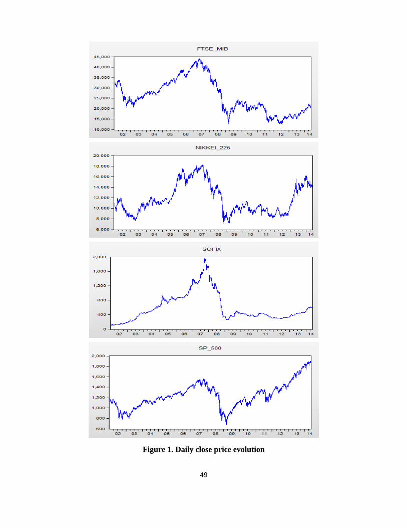
49

Figure 1. Daily close price evolution

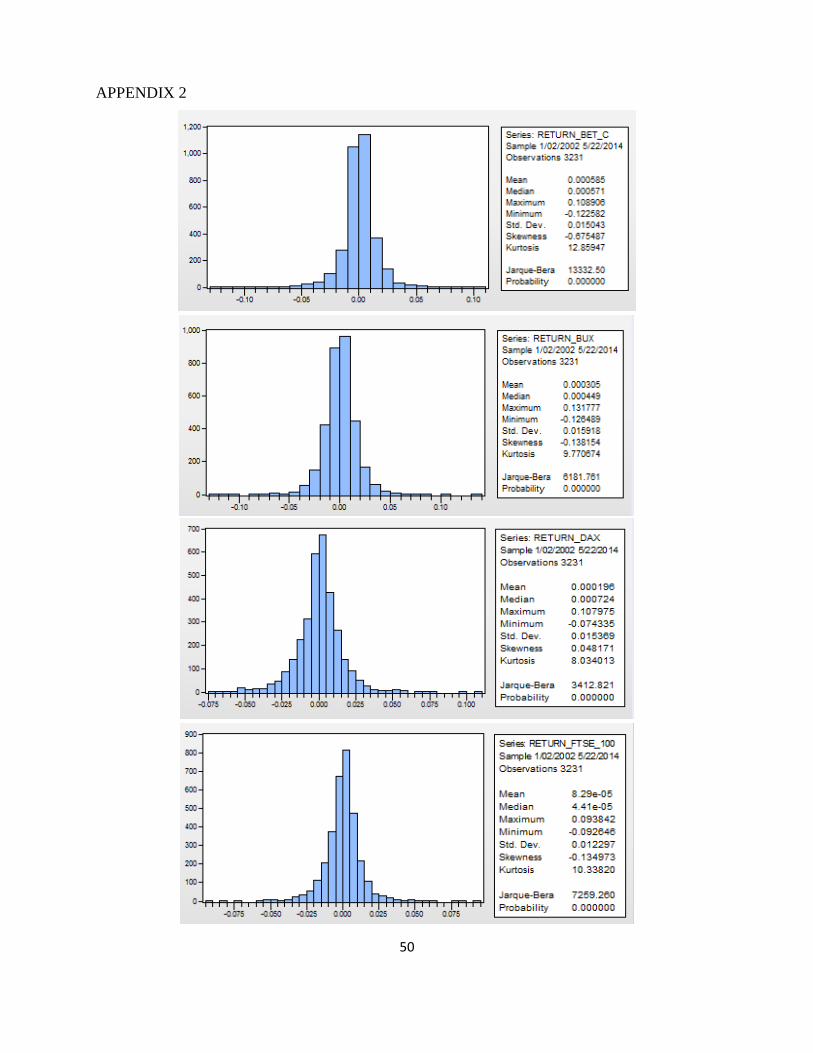
50

APPENDIX 2

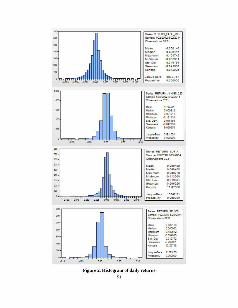
51

Figure 2. Histogram of daily returns

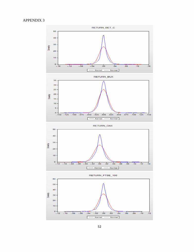
52

APPENDIX 3

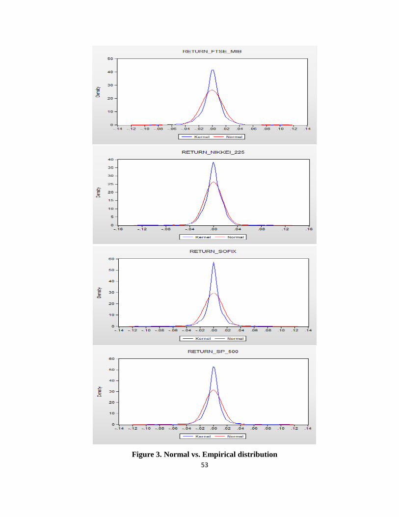
53

Figure 3. Normal vs. Empirical distribution

54

APPENDIX 4

Figure 4. Q-Q Plot

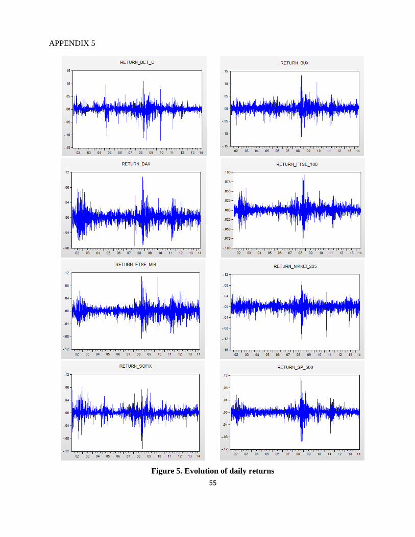
55

APPENDIX 5

Figure 5. Evolution of daily returns

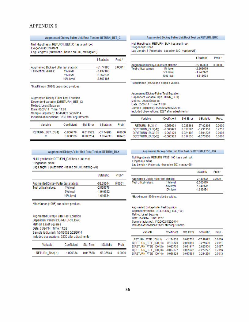
56

APPENDIX 6

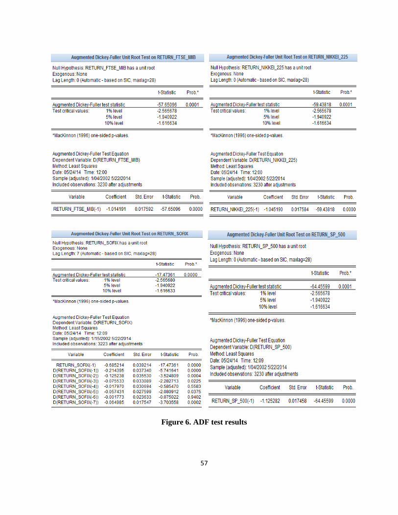
57

Figure 6. ADF test results

58

APPENDIX 7

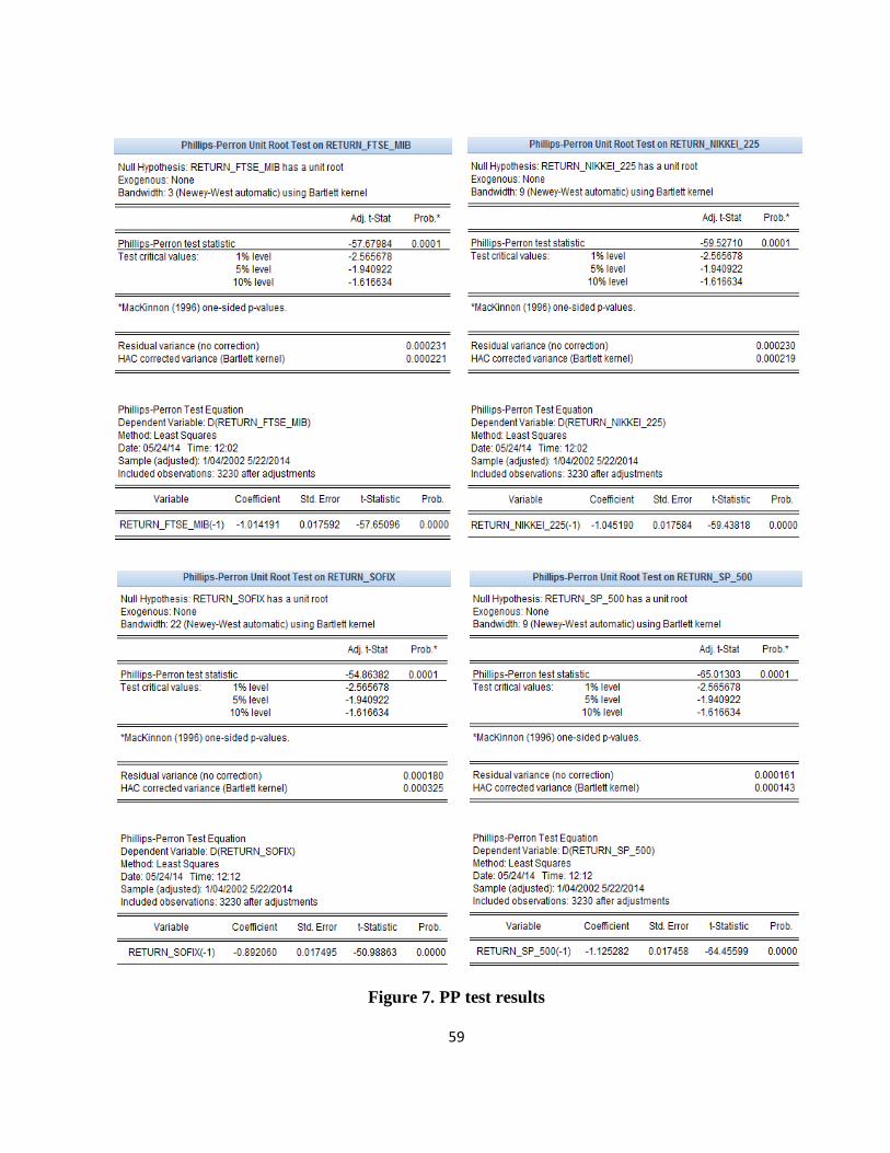
59

Figure 7. PP test results

60

APPENDIX 8

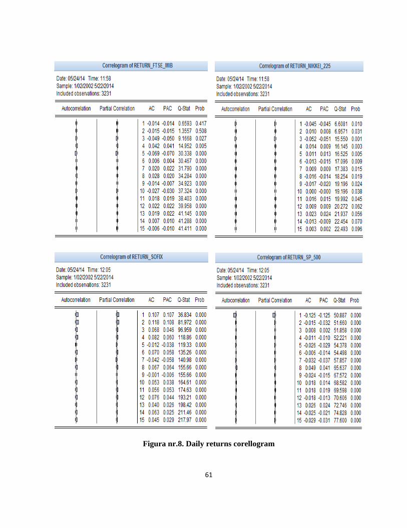
61

Figura nr.8. Daily returns corellogram

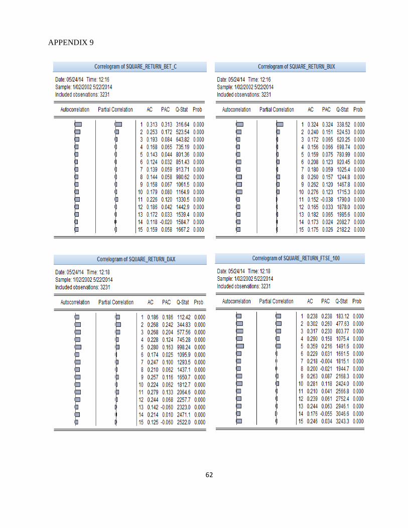
62

APPENDIX 9

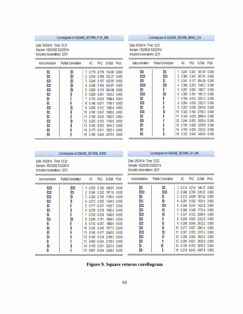
63

Figure 9. Square returns corellogram

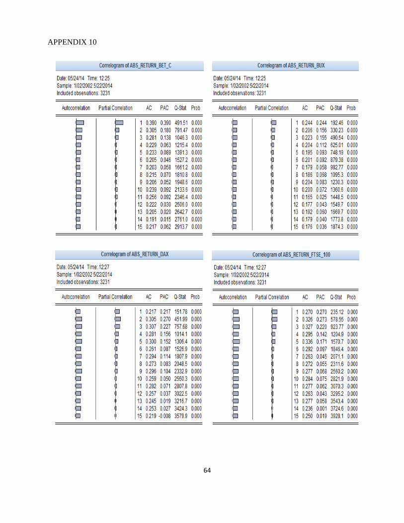
64

APPENDIX 10

65

Figure 10. Absolute returns corellogram

66

APPENDIX 11

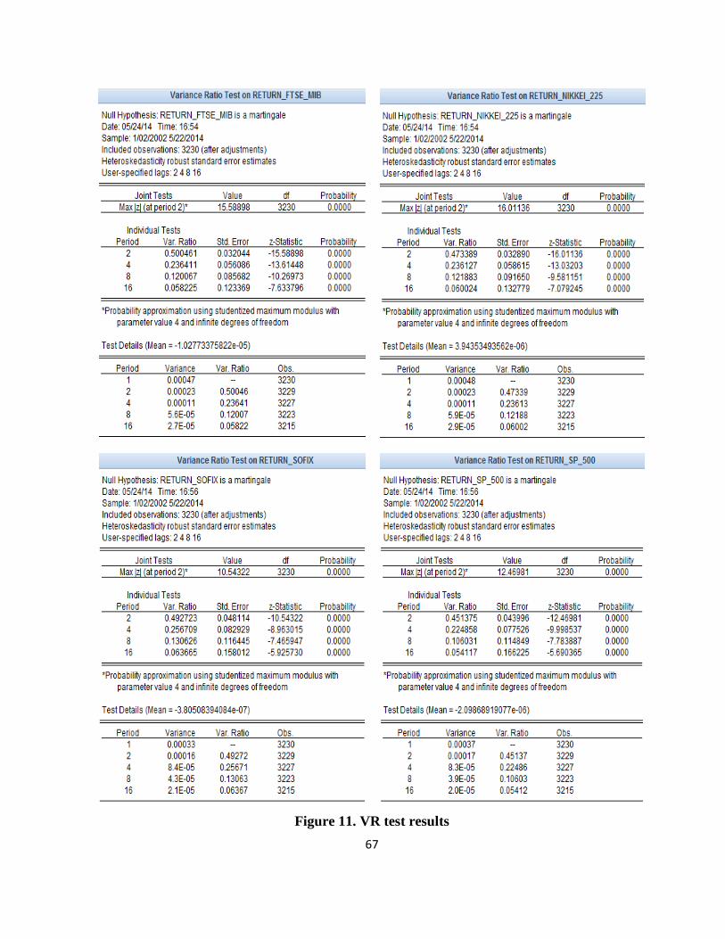
67

Figure 11. VR test results

68

APPENDIX 12

0 1 2 4 5

n

m

Akaike -5.555547 -5.563302 -5.555593 -5.555286 -5.555559

0 Schwarz -5.553665 -5.559538 -5.551829 -5.551522 -5.551795

Log likelihood 8975.986 8989.514 8977.061 8976.564 8977.006

R2 0.000000 0.008339 0.000665 0.000358 0.000631

Akaike -5.563557 -5.562656 -5.563252 -5.563410 -5.563003

1 Schwarz -5.559792 -5.558891 -5.557605 -5.557762 -5.559238

Log likelihood 8987.145 8985.689 8987.652 8987.907 8986.249

R2 0.008692 0.007798 0.009003 0.009159 0.008142

Akaike -5.555336 -5.562506 -5.554577 -5.555142 -5.555366

2 Schwarz -5.551570 -5.558740 -5.550811 -5.549493 -5.549718

Log likelihood 8971.089 8982.666 8969.865 8971.776 8972.139

R2 0.000637 0.007778 -0.000121 0.001063 0.001287

Akaike -5.554477 -5.562305 -5.554552 -5.554661 -5.554634

4 Schwarz -5.550710 -5.556653 -5.548901 -5.549010 -5.548983

R2 8964.149 8977.779 8965.270 8965.446 8965.403

R-squared 0.000386 0.008794 0.001080 0.001189 0.001162

Akaike -5.555130 -5.562331 -5.555207 -5.554977 -5.561991

5 Schwarz -5.551361 -5.558563 -5.549554 -5.549324 -5.558222

Log likelihood 8962.424 8974.041 8963.549 8963.178 8973.491

R-squared 0.000668 0.007839 0.001365 0.001135 0.007501

Figure 12.1. ARMA - BET-C

0 1 2 4 6

n

m

Akaike -5.442397 -5.443294 -5.445023 -5.448646 -5.444391

0 Schwarz -5.440515 -5.441412 -5.443141 -5.446764 -5.442509

Log likelihood 8793.192 8794.641 8797.435 8803.288 8796.413

R2 0.000000 0.000897 0.002623 0.006230 0.001992

Akaike -5.442884 -5.443374 -5.445325 -5.448875 -5.444751

1 Schwarz -5.441001 -5.439609 -5.441560 -5.445110 -5.440986

Log likelihood 8791.257 8793.049 8796.200 8801.933 8795.273

R2 0.000753 0.001861 0.003807 0.007337 0.003235

Akaike -5.445593 -5.446146 -5.453844 -5.450685 -5.446827

2 Schwarz -5.443711 -5.442380 -5.450078 -5.446919 -5.443061

Log likelihood 8792.911 8794.803 8807.231 8802.131 8795.902

R2 0.003111 0.004279 0.011914 0.008788 0.004956

Akaike -5.448318 -5.448945 -5.450289 -5.449646 -5.449386

4 Schwarz -5.446435 -5.445177 -5.446521 -5.445878 -5.445618

R2 8791.862 8793.872 8796.041 8795.004 8794.584

R-squared 0.006436 0.007673 0.009006 0.008369 0.008111

Akaike -5.444134 -5.444801 -5.446051 -5.449373 -5.445155

6 Schwarz -5.442249 -5.441031 -5.442281 -5.445603 -5.441385

Log likelihood 8779.666 8781.741 8783.757 8789.114 8782.312

R-squared 0.002171 0.003454 0.004699 0.008000 0.003806

Figure 12.2. ARMA - BUX

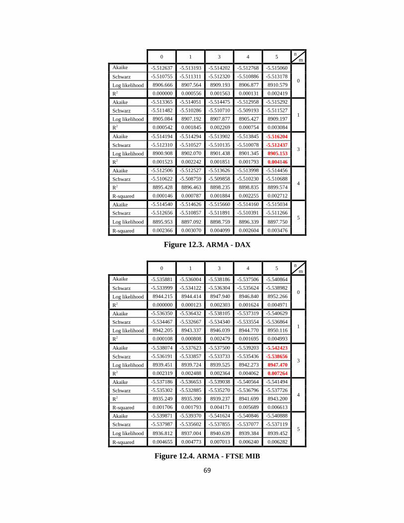
69

0 1 3 4 5

n m

Akaike -5.512637 -5.513193 -5.514202 -5.512768 -5.515060

0 Schwarz -5.510755 -5.511311 -5.512320 -5.510886 -5.513178

Log likelihood 8906.666 8907.564 8909.193 8906.877 8910.579

R2 0.000000 0.000556 0.001563 0.000131 0.002419

Akaike -5.513365 -5.514051 -5.514475 -5.512958 -5.515292

1 Schwarz -5.511482 -5.510286 -5.510710 -5.509193 -5.511527

Log likelihood 8905.084 8907.192 8907.877 8905.427 8909.197

R2 0.000542 0.001845 0.002269 0.000754 0.003084

Akaike -5.514194 -5.514294 -5.513902 -5.513845 -5.516204

3 Schwarz -5.512310 -5.510527 -5.510135 -5.510078 -5.512437

Log likelihood 8900.908 8902.070 8901.438 8901.345 8905.153

R2 0.001523 0.002242 0.001851 0.001793 0.004146

Akaike -5.512506 -5.512527 -5.513626 -5.513998 -5.514456

4 Schwarz -5.510622 -5.508759 -5.509858 -5.510230 -5.510688

R2 8895.428 8896.463 8898.235 8898.835 8899.574

R-squared 0.000146 0.000787 0.001884 0.002255 0.002712

Akaike -5.514540 -5.514626 -5.515660 -5.514160 -5.515034

5 Schwarz -5.512656 -5.510857 -5.511891 -5.510391 -5.511266

Log likelihood 8895.953 8897.092 8898.759 8896.339 8897.750

R-squared 0.002366 0.003070 0.004099 0.002604 0.003476

Figure 12.3. ARMA - DAX

0 1 3 4 5

n m

Akaike -5.535881 -5.536004 -5.538186 -5.537506 -5.540864

0 Schwarz -5.533999 -5.534122 -5.536304 -5.535624 -5.538982

Log likelihood 8944.215 8944.414 8947.940 8946.840 8952.266

R2 0.000000 0.000123 0.002303 0.001624 0.004971

Akaike -5.536350 -5.536432 -5.538105 -5.537319 -5.540629

1 Schwarz -5.534467 -5.532667 -5.534340 -5.533554 -5.536864

Log likelihood 8942.205 8943.337 8946.039 8944.770 8950.116

R2 0.000108 0.000808 0.002479 0.001695 0.004993

Akaike -5.538074 -5.537623 -5.537500 -5.539203 -5.542423

3 Schwarz -5.536191 -5.533857 -5.533733 -5.535436 -5.538656

Log likelihood 8939.451 8939.724 8939.525 8942.273 8947.470

R2 0.002319 0.002488 0.002364 0.004062 0.007264

Akaike -5.537186 -5.536653 -5.539038 -5.540564 -5.541494

4 Schwarz -5.535302 -5.532885 -5.535270 -5.536796 -5.537726

R2 8935.249 8935.390 8939.237 8941.699 8943.200

R-squared 0.001706 0.001793 0.004171 0.005689 0.006613

Akaike -5.539871 -5.539370 -5.541624 -5.540846 -5.540888

5 Schwarz -5.537987 -5.535602 -5.537855 -5.537077 -5.537119

Log likelihood 8936.812 8937.004 8940.639 8939.384 8939.452

R-squared 0.004655 0.004773 0.007013 0.006240 0.006282

Figure 12.4. ARMA - FTSE MIB

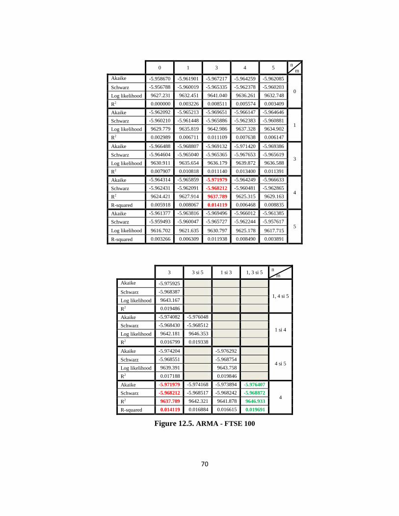
70

0 1 3 4 5

n m

Akaike -5.958670 -5.961901 -5.967217 -5.964259 -5.962085

0 Schwarz -5.956788 -5.960019 -5.965335 -5.962378 -5.960203

Log likelihood 9627.231 9632.451 9641.040 9636.261 9632.748

R2 0.000000 0.003226 0.008511 0.005574 0.003409

Akaike -5.962092 -5.965213 -5.969651 -5.966147 -5.964646

1 Schwarz -5.960210 -5.961448 -5.965886 -5.962383 -5.960881

Log likelihood 9629.779 9635.819 9642.986 9637.328 9634.902

R2 0.002989 0.006711 0.011109 0.007638 0.006147

Akaike -5.966488 -5.968807 -5.969132 -5.971420 -5.969386

3 Schwarz -5.964604 -5.965040 -5.965365 -5.967653 -5.965619

Log likelihood 9630.911 9635.654 9636.179 9639.872 9636.588

R2 0.007907 0.010818 0.011140 0.013400 0.011391

Akaike -5.964314 -5.965859 -5.971979 -5.964249 -5.966633

4 Schwarz -5.962431 -5.962091 -5.968212 -5.960481 -5.962865

R2 9624.421 9627.914 9637.789 9625.315 9629.163

R-squared 0.005918 0.008067 0.014119 0.006468 0.008835

Akaike -5.961377 -5.963816 -5.969496 -5.966012 -5.961385

5 Schwarz -5.959493 -5.960047 -5.965727 -5.962244 -5.957617

Log likelihood 9616.702 9621.635 9630.797 9625.178 9617.715

R-squared 0.003266 0.006309 0.011938 0.008490 0.003891

3 3 si 5 1 si 3 1, 3 si 5

n

m

Akaike -5.975925

1, 4 si 5 Schwarz -5.968387

Log likelihood 9643.167

R2 0.019486

Akaike -5.974082 -5.976048

1 si 4 Schwarz -5.968430 -5.968512

Log likelihood 9642.181 9646.353

R2 0.016799 0.019338

Akaike -5.974204 -5.976292

4 si 5 Schwarz -5.968551 -5.968754


R2 0.017188 0.019846

Akaike -5.971979 -5.974168 -5.973894 -5.976407

4 Schwarz -5.968212 -5.968517 -5.968242 -5.968872

R2 9637.789 9642.321 9641.878 9646.933

R-squared 0.014119 0.016884 0.016615 0.019691

Figure 12.5. ARMA - FTSE 100

71

0 1 2 3 4

n

m

Akaike -5.535568 -5.537541 -5.535632 -5.538276 -5.535718

0 Schwarz -5.533686 -5.535659 -5.533750 -5.536394 -5.533836

Log likelihood 8943.709 8946.897 8943.814 8948.085 8943.953

R2 0.000000 0.001971 0.000065 0.002705 0.000151

Akaike -5.537348 -5.537645 -5.536764 -5.539360 -5.536875

1 Schwarz -5.535465 -5.533880 -5.532999 -5.535595 -5.533110

Log likelihood 8943.816 8945.296 8943.874 8948.067 8944.053

R2 0.002002 0.002916 0.002038 0.004625 0.002148

Akaike -5.536370 -5.537778 -5.535993 -5.538431 -5.535958

2 Schwarz -5.534487 -5.534013 -5.532227 -5.534665 -5.532192

Log likelihood 8939.469 8942.743 8939.861 8943.797 8939.804

R2 0.000077 0.002103 0.000319 0.002754 0.000285

Akaike -5.538669 -5.540014 -5.538139 -5.538446 -5.538209

3 Schwarz -5.536785 -5.536248 -5.534372 -5.534679 -5.534442

R2 8940.411 8943.583 8940.556 8941.051 8940.669

R-squared 0.002627 0.004585 0.002717 0.003023 0.002786

Akaike -5.536582 -5.537982 -5.536083 -5.538652 -5.539219

4 Schwarz -5.534698 -5.534215 -5.532315 -5.534884 -5.535451

Log likelihood 8934.275 8937.534 8934.470 8938.614 8939.530

R-squared 0.000150 0.002167 0.000271 0.002835 0.003401

Figure 12.6. ARMA - NIKKEI 225

0 1 2 5 8

n m

Akaike -5.882762 -5.899205 -5.882859 -5.883257 -5.884887

0 Schwarz -5.880880 -5.897323 -5.880977 -5.881375 -5.883005

Log likelihood 9504.602 9531.166 9504.758 9505.401 9508.035

R2 0.000000 0.016309 0.000097 0.000495 0.002123

Akaike -5.898290 -5.898680 -5.898653 -5.898463 -5.899436

1 Schwarz -5.896407 -5.894916 -5.894888 -5.894699 -5.895671

Log likelihood 9526.738 9528.369 9528.325 9528.018 9529.589

R2 0.015562 0.016556 0.016529 0.016342 0.017298

Akaike -5.882465 -5.898420 -5.881846 -5.882499 -5.884149

2 Schwarz -5.880582 -5.894654 -5.878081 -5.878733 -5.880383

Log likelihood 9498.240 9524.999 9498.241 9499.294 9501.958

R2 0.000100 0.016536 0.000101 0.000753 0.002401

Akaike -5.882109 -5.898298 -5.881751 -5.882263 -5.883868

5 Schwarz -5.880224 -5.894530 -5.877982 -5.878494 -5.880099

R2 9488.841 9515.955 9489.265 9490.090 9492.679

R-squared 0.000516 0.017176 0.000778 0.001289 0.002891

Akaike -5.883188 -5.898672 -5.882830 -5.883308 -5.882979

8 Schwarz -5.881302 -5.894900 -5.879058 -5.879536 -5.879208

Log likelihood 9481.757 9507.709 9482.181 9482.951 9482.421

R-squared 0.002265 0.018204 0.002527 0.003004 0.002676

Figure 12.7. ARMA - S&P 500

72

0 1 2 4 6

n

m

Akaike -5.771775 -5.780023 -5.783069 -5.776710 -5.774912

0 Schwarz -5.769893 -5.778141 -5.781187 -5.774829 -5.773030

Log likelihood 9325.303 9338.627 9343.548 9333.276 9330.370

R2 0.000000 0.008214 0.011231 0.004923 0.003132

Akaike -5.781823 -5.798788 -5.790819 -5.786786 -5.786786

1 Schwarz -5.779940 -5.795023 -5.787054 -5.783021 -5.783022

Log likelihood 9338.644 9367.042 9354.173 9347.660 9347.660

R2 0.010304 0.027555 0.019775 0.015813 0.015814

Akaike -5.788402 -5.796229 -5.803634 -5.791544 -5.790308

2 Schwarz -5.786519 -5.792463 -5.799868 -5.787779 -5.786542

Log likelihood 9346.375 9360.012 9371.967 9352.449 9350.452

R2 0.012873 0.021176 0.028397 0.016579 0.015362

Akaike -5.780473 -5.789172 -5.791362 -5.791750 -5.782732

4 Schwarz -5.778589 -5.785404 -5.787594 -5.787982 -5.778964

R2 9327.792 9342.829 9346.363 9346.988 9332.438

R-squared 0.005553 0.014777 0.016932 0.017313 0.008412

Akaike -5.778089 -5.788266 -5.788331 -5.782323 -5.788015

6 Schwarz -5.776204 -5.784497 -5.784561 -5.778554 -5.784245

Log likelihood 9318.168 9335.580 9335.684 9325.996 9335.174

R-squared 0.003685 0.014385 0.014449 0.008510 0.014137

2 2 si 5 1 si 2 1, 2 si 5

n

m

Akaike -5.814182

1, 2 si 5 Schwarz -5.806644

Log likelihood 9382.275

R2 0.040529

Akaike -5.806947 -5.819696

1 si 2 Schwarz -5.801298 -5.812165


R2 0.03221 0.045062

Akaike -5.804322 -5.811911

2 si 5 Schwarz -5.798669 -5.804373


R2 0.030421 0.038347

Akaike -5.803634 -5.804049 -5.806926 -5.814646

2 Schwarz -5.799868 -5.7984 -5.801277 -5.807114

R2 9371.967 9373.636 9378.282 9391.746

R-squared 0.028397 0.029401 0.03219 0.040227

Figure 12.8. ARMA - SOFIX

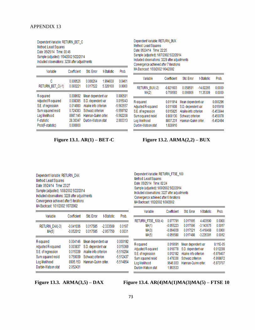
73

APPENDIX 13

Figure 13.1. AR(1) – BET-C Figure 13.2. ARMA(2,2) – BUX

Figure 13.3. ARMA(3,5) – DAX Figure 13.4. AR(4)MA(1)MA(3)MA(5) – FTSE 10

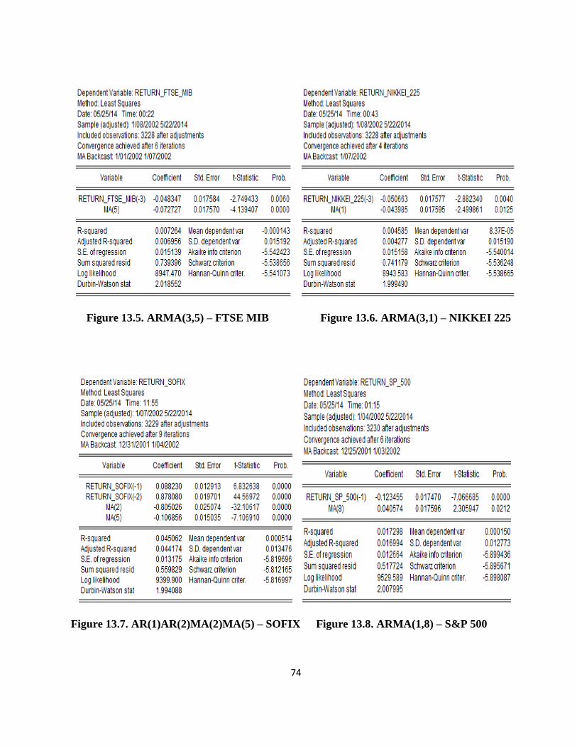
74

Figure 13.5. ARMA(3,5) – FTSE MIB Figure 13.6. ARMA(3,1) – NIKKEI 225

Figure 13.7. AR(1)AR(2)MA(2)MA(5) – SOFIX Figure 13.8. ARMA(1,8) – S&P 500

75

APPENDIX 14

Figure 14.1. AR(1) – BET-C correlogram Figure 14.2. ARMA(2,2) – BUX correlogram

Figure 14.3. ARMA(3,5) – DAX correlogram Figure 14.4. AR(4)MA(1)MA(3)MA(5) –

FTSE correlogram

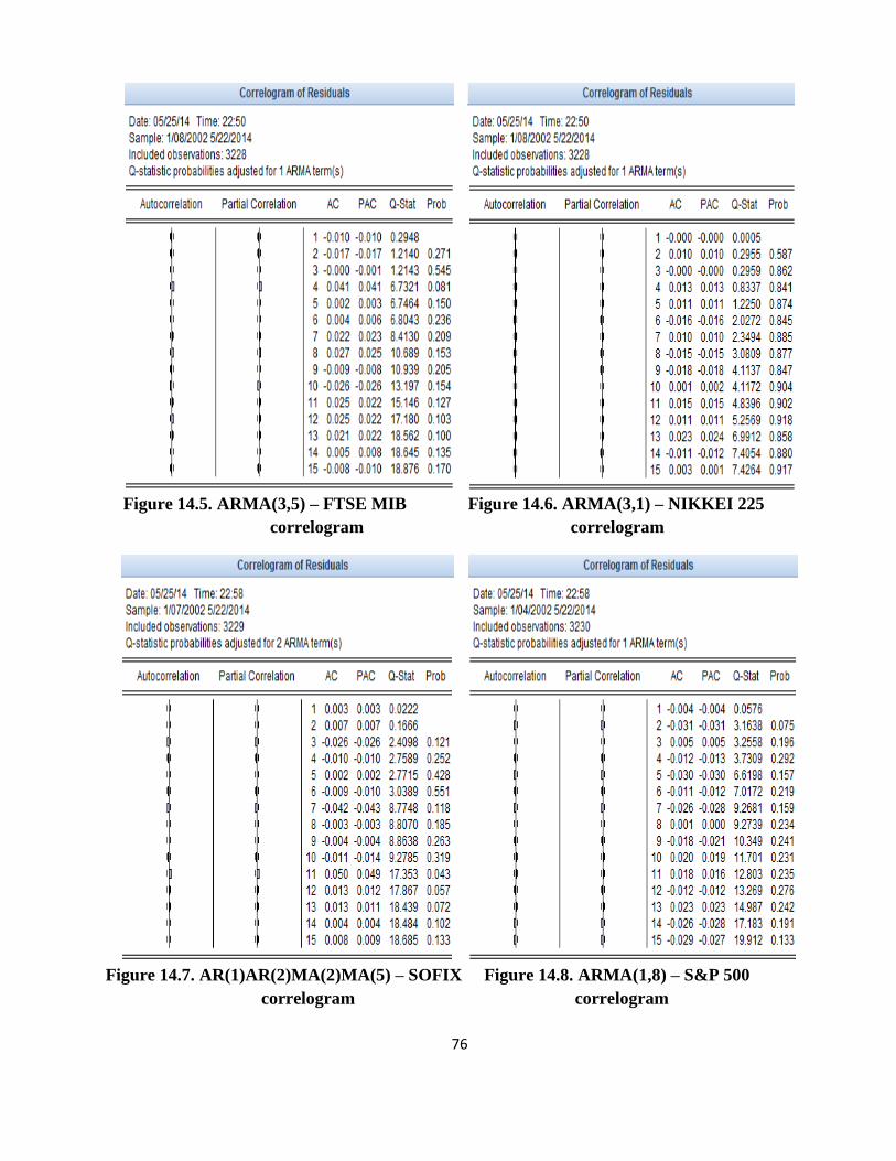
76

Figure 14.5. ARMA(3,5) – FTSE MIB Figure 14.6. ARMA(3,1) – NIKKEI 225

correlogram correlogram

Figure 14.7. AR(1)AR(2)MA(2)MA(5) – SOFIX Figure 14.8. ARMA(1,8) – S&P 500

correlogram correlogram

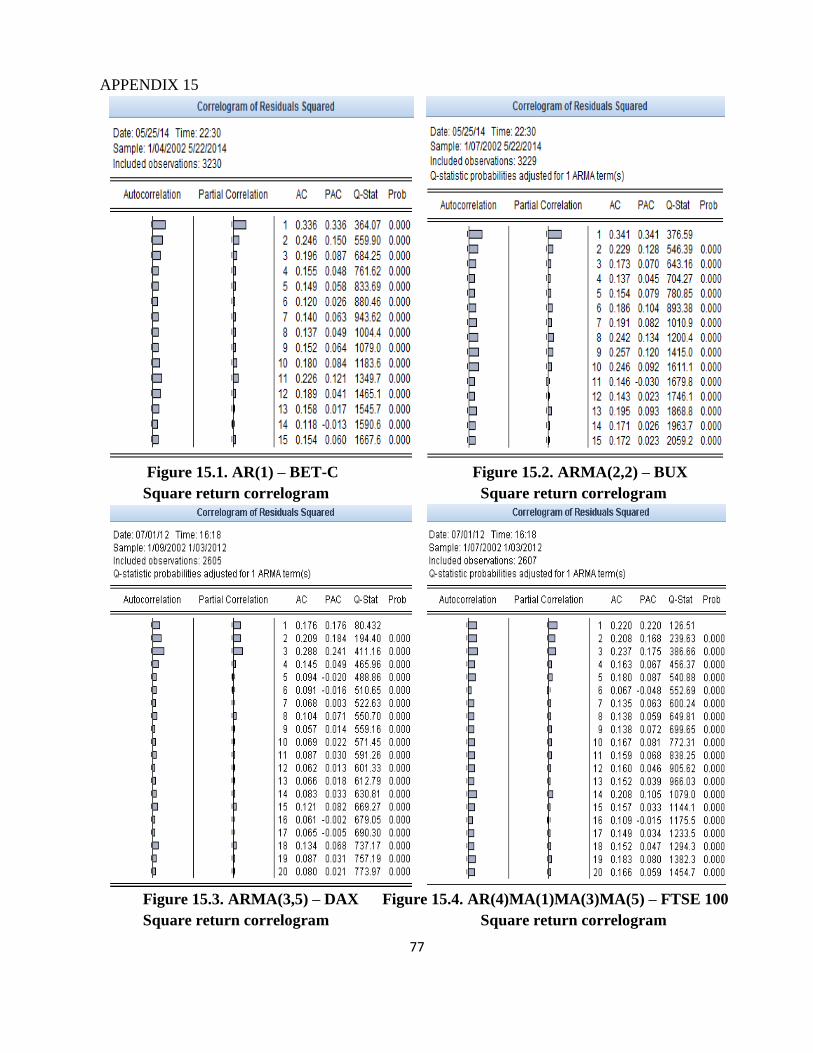
77

APPENDIX 15

Figure 15.1. AR(1) – BET-C Figure 15.2. ARMA(2,2) – BUX

Square return correlogram Square return correlogram

Figure 15.3. ARMA(3,5) – DAX Figure 15.4. AR(4)MA(1)MA(3)MA(5) – FTSE 100


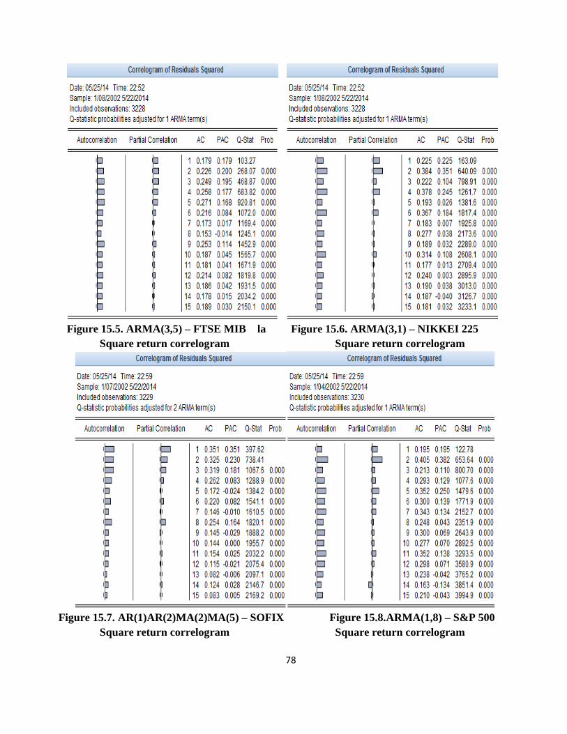
78

Figure 15.5. ARMA(3,5) – FTSE MIB la Figure 15.6. ARMA(3,1) – NIKKEI 225


Figure 15.7. AR(1)AR(2)MA(2)MA(5) – SOFIX Figure 15.8.ARMA(1,8) – S&P 500


79

APPENDIX 16

Figure 16.1. ARCH test results Figure 16.2. ARCH test results

AR(1) – BET-C ARMA(2,2) – BUX


ARMA(3,5) – DAX AR(4)MA(1)MA(3)MA(5) – FTSE 100

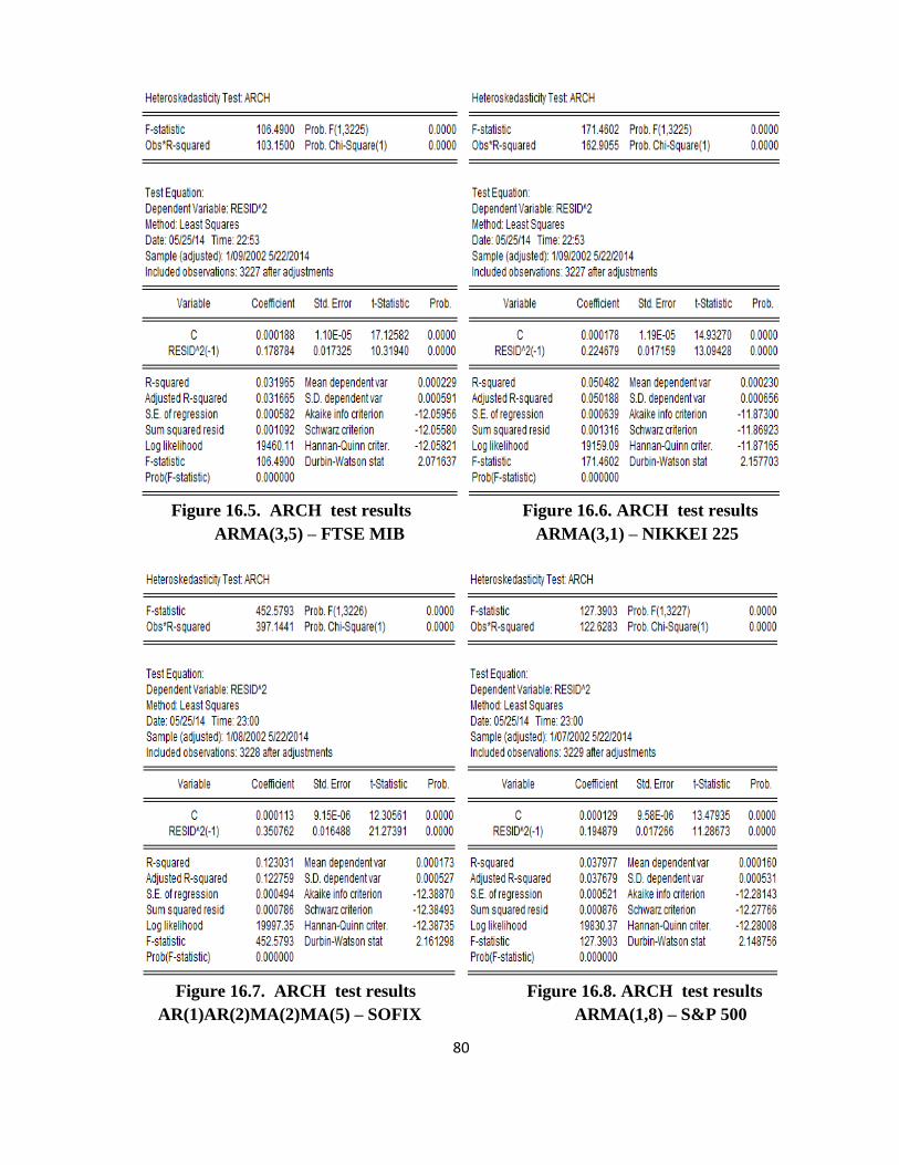
80


ARMA(3,5) – FTSE MIB ARMA(3,1) – NIKKEI 225


AR(1)AR(2)MA(2)MA(5) – SOFIX ARMA(1,8) – S&P 500

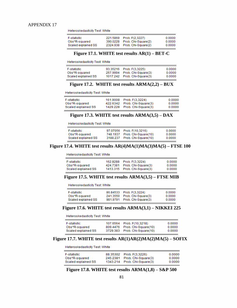
81

APPENDIX 17

Figure 17.1. WHITE test results AR(1) – BET-C

Figure 17.2. WHITE test results ARMA(2,2) – BUX

Figure 17.3. WHITE test results ARMA(3,5) – DAX

Figure 17.4. WHITE test results AR(4)MA(1)MA(3)MA(5) – FTSE 100

Figure 17.5. WHITE test results ARMA(3,5) – FTSE MIB

Figure 17.6. WHITE test results ARMA(3,1) – NIKKEI 225

Figure 17.7. WHITE test results AR(1)AR(2)MA(2)MA(5) – SOFIX

Figure 17.8. WHITE test results ARMA(1,8) – S&P 500

82

APPENDIX 18

Figure 18.1. BG test results AR(1) – BET-C

Figure 18.2. BG test results ARMA(2,2) – BUX

Figure 18.3. BG test results ARMA(3,5) – DAX

Figure 18.4. BG test results AR(4)MA(1)MA(3)MA(5) – FTSE 100

Figure 18.5. BG test results ARMA(3,5) – FTSE MIB

Figure 18.6. BG test results ARMA(3,1) – NIKKEI 225

Figure 18.7. BG test results AR(1)AR(2)MA(2)MA(5) – SOFIX

Figure 18.9. BG test results ARMA(1,8) – S&P 500

83

APPENDIX 19

Figure 19.3 AR(1) – BET-C Histogram

Figure 19.3 ARMA(2,2) – BUX Histogram

Figure 19.3. ARMA(3,5) – DAX Histogram

Figure 19.4. AR(4)MA(1)MA(3)MA(5) – FTSE 100 Histogram

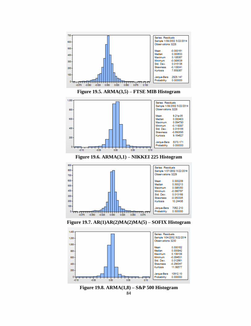
84

Figure 19.5. ARMA(3,5) – FTSE MIB Histogram

Figure 19.6. ARMA(3,1) – NIKKEI 225 Histogram

Figure 19.7. AR(1)AR(2)MA(2)MA(5) – SOFIX Histogram

Figure 19.8. ARMA(1,8) – S&P 500 Histogram

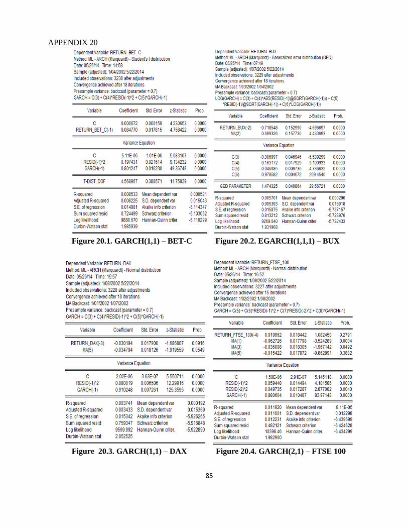
85

APPENDIX 20

Figure 20.1. GARCH(1,1) – BET-C Figure 20.2. EGARCH(1,1,1) – BUX

Figure 20.3. GARCH(1,1) – DAX Figure 20.4. GARCH(2,1) – FTSE 100

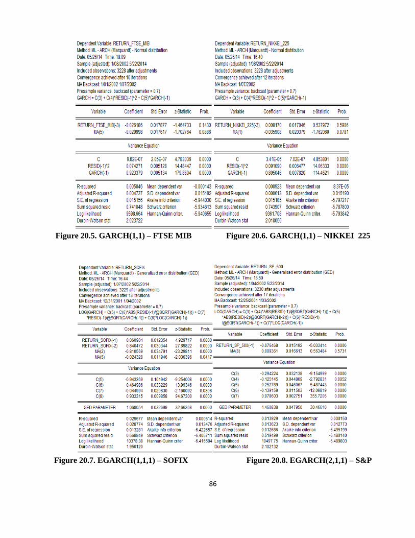
86

Figure 20.5. GARCH(1,1) – FTSE MIB Figure 20.6. GARCH(1,1) – NIKKEI 225

Figure 20.7. EGARCH(1,1,1) – SOFIX Figure 20.8. EGARCH(2,1,1) – S&P

87

APPENDIX 21

Figure 21. Wald test results

88

APPENDIX 22

Figure 22.1. GARCH(1,1) – BET-C Figure 22.2. EGARCH(1,1,1) – BUX




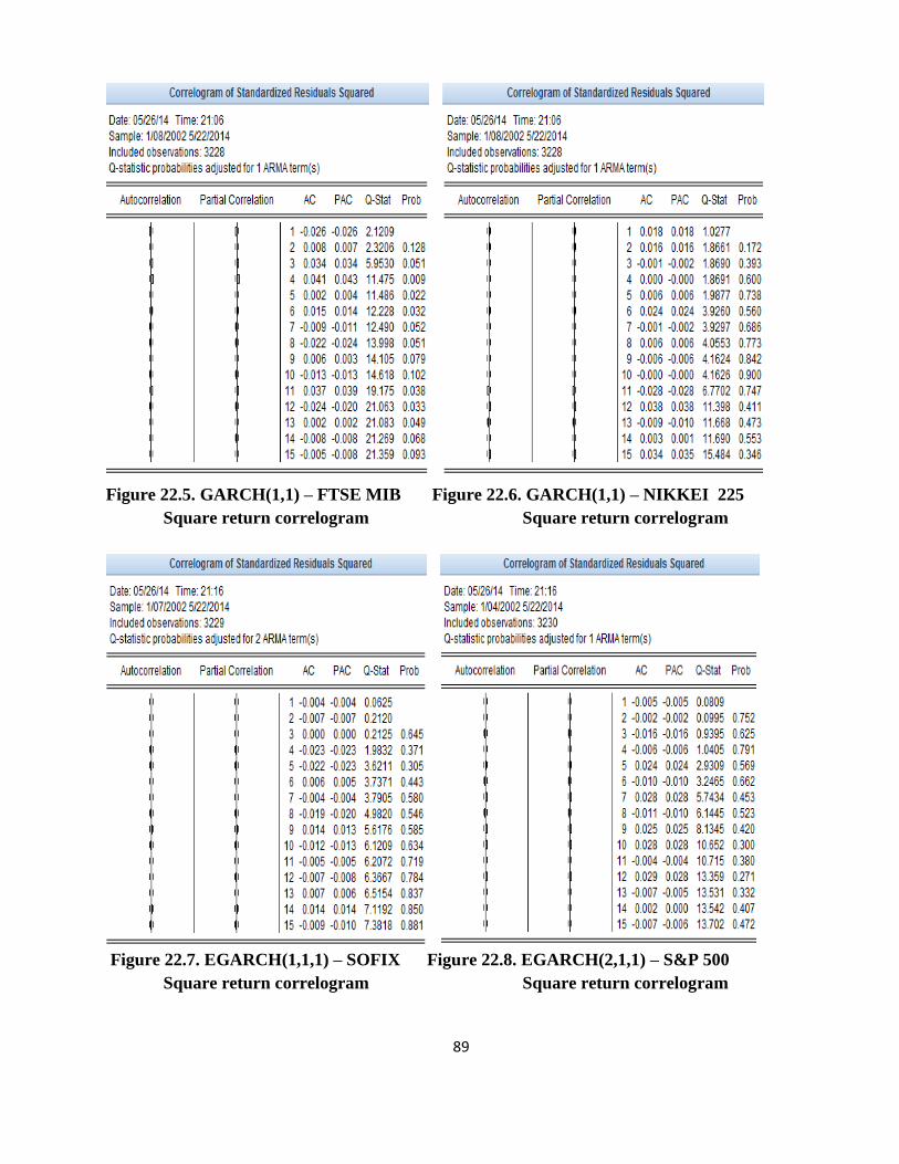
89



Figure 22.7. EGARCH(1,1,1) – SOFIX Figure 22.8. EGARCH(2,1,1) – S&P 500


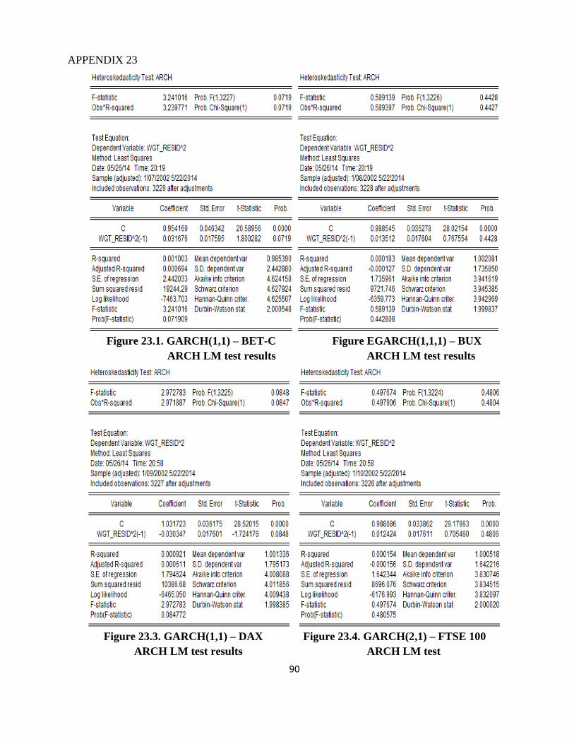
90

APPENDIX 23

Figure 23.1. GARCH(1,1) – BET-C Figure EGARCH(1,1,1) – BUX

ARCH LM test results ARCH LM test results


ARCH LM test results ARCH LM test

91



Figure 23.7. EGARCH(1,1,1) – SOFIX Figure 23.8. EGARCH(2,1,1) – S&P 500


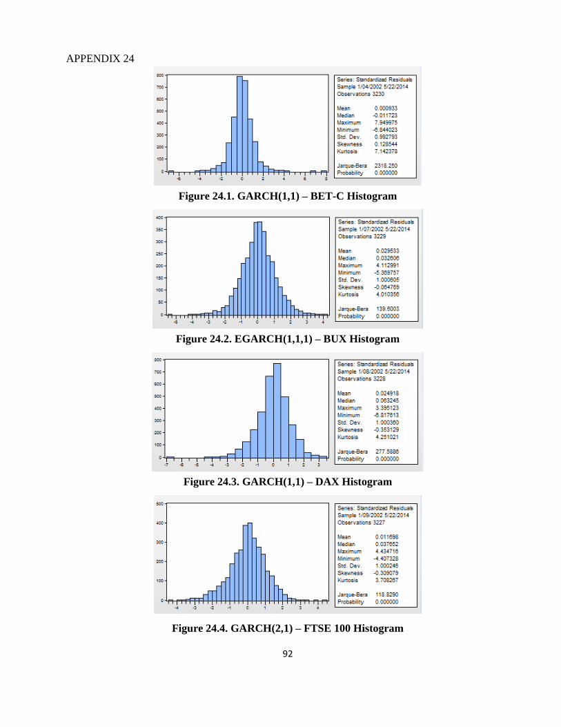
92

APPENDIX 24

Figure 24.1. GARCH(1,1) – BET-C Histogram

Figure 24.2. EGARCH(1,1,1) – BUX Histogram

Figure 24.3. GARCH(1,1) – DAX Histogram

Figure 24.4. GARCH(2,1) – FTSE 100 Histogram

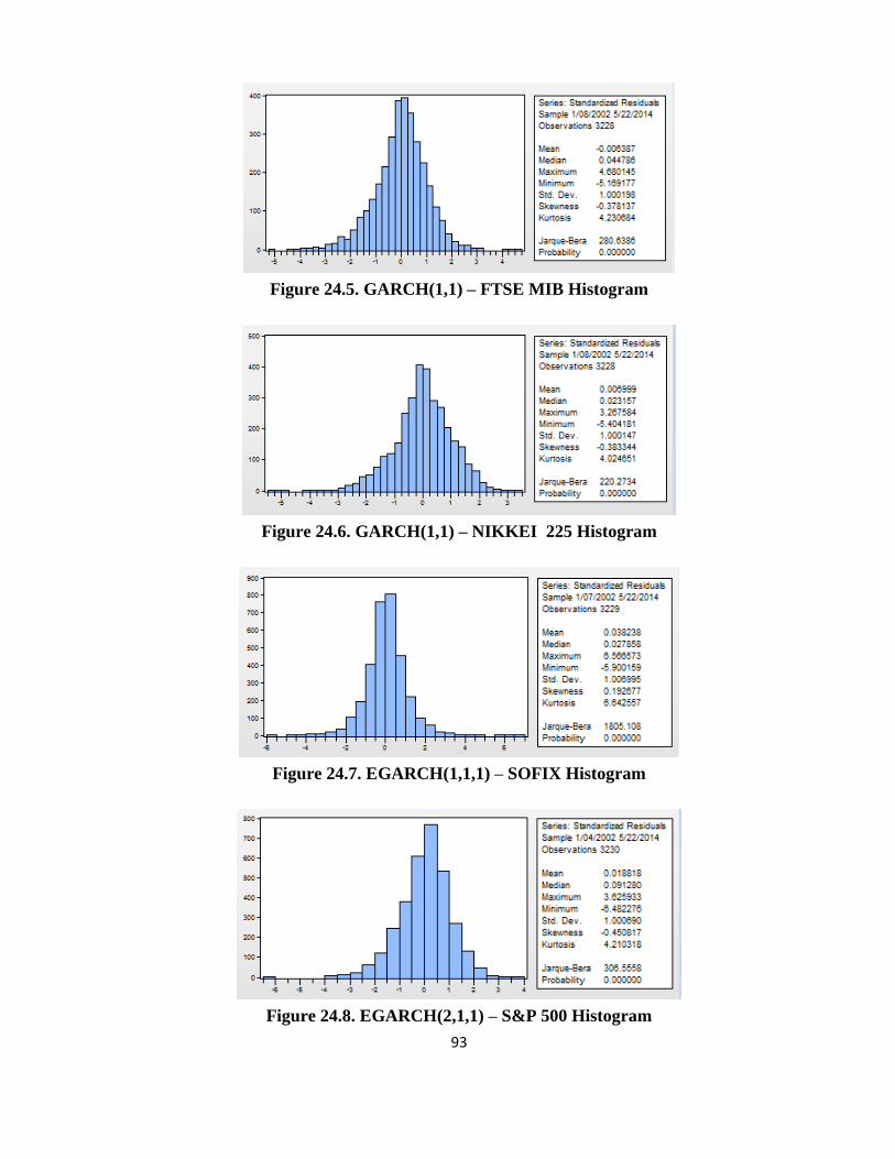
93

Figure 24.5. GARCH(1,1) – FTSE MIB Histogram

Figure 24.6. GARCH(1,1) – NIKKEI 225 Histogram

Figure 24.7. EGARCH(1,1,1) – SOFIX Histogram

Figure 24.8. EGARCH(2,1,1) – S&P 500 Histogram

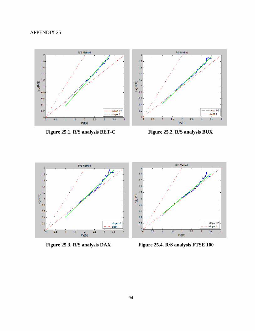
94

APPENDIX 25

Figure 25.1. R/S analysis BET-C Figure 25.2. R/S analysis BUX

Figure 25.3. R/S analysis DAX Figure 25.4. R/S analysis FTSE 100

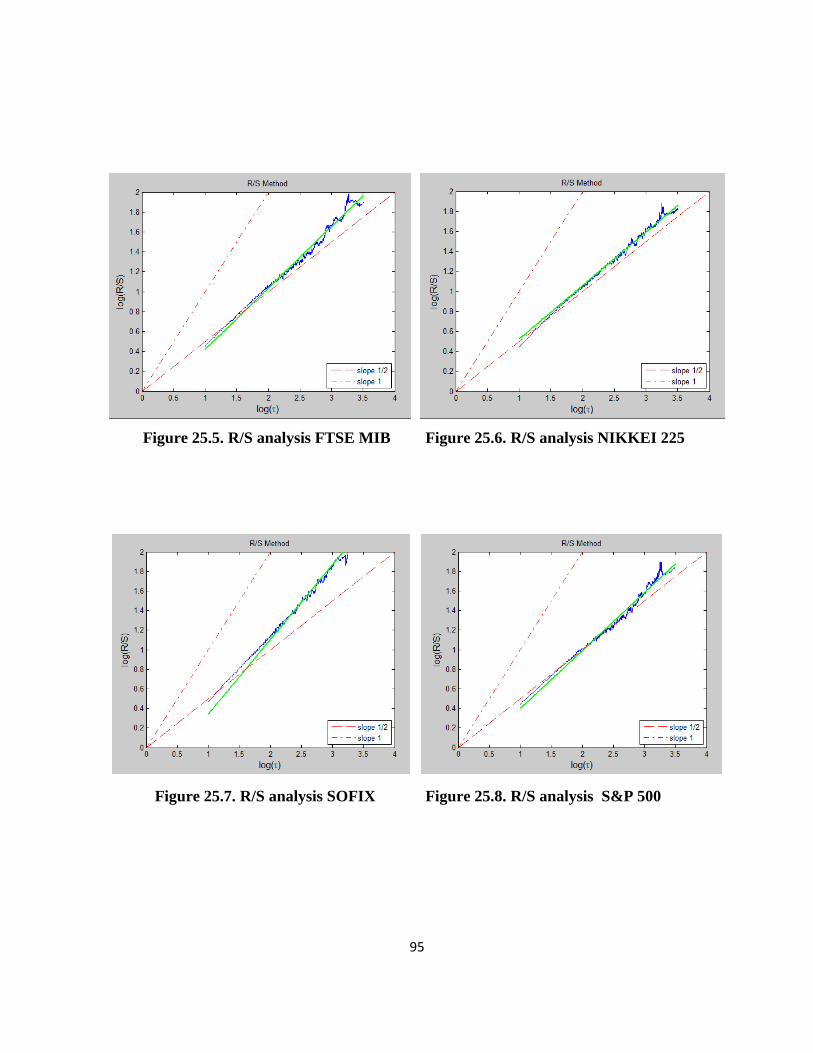
95

Figure 25.5. R/S analysis FTSE MIB Figure 25.6. R/S analysis NIKKEI 225

Figure 25.7. R/S analysis SOFIX Figure 25.8. R/S analysis S&P 500

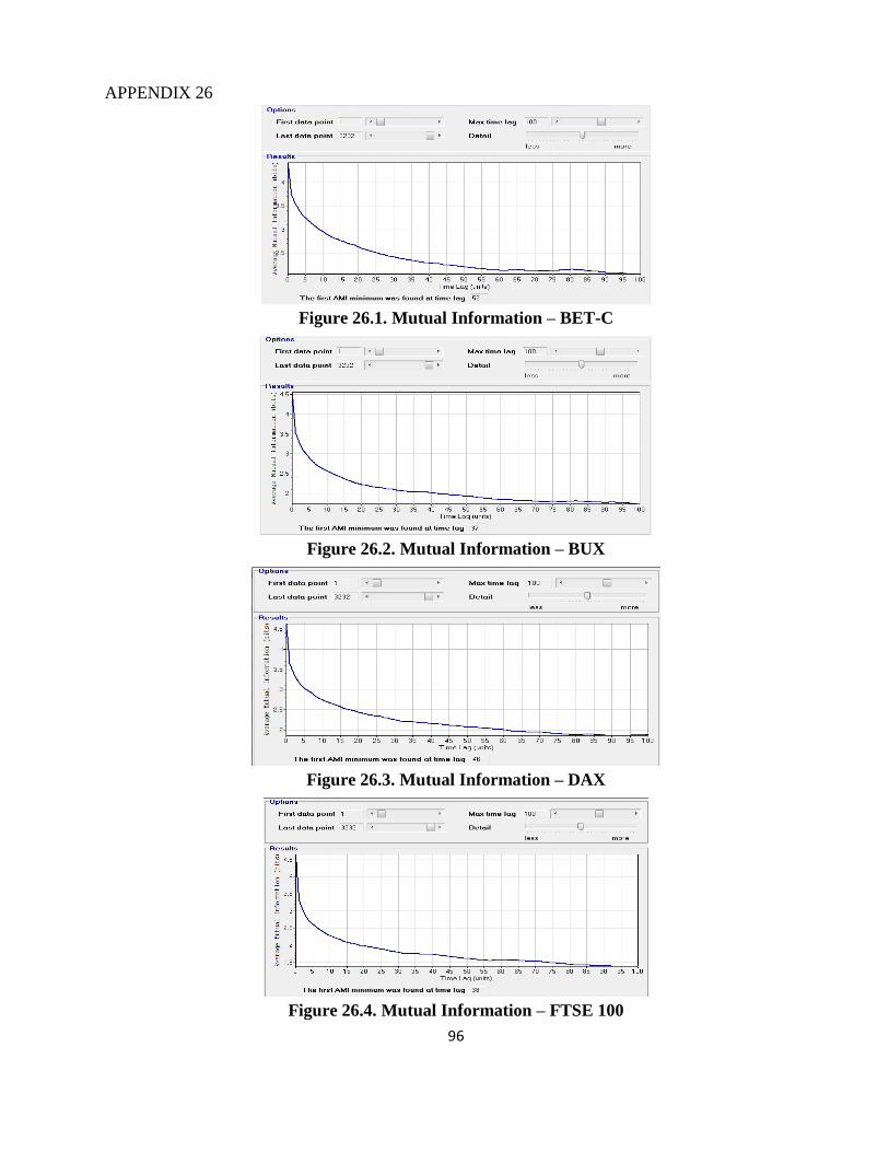
96

APPENDIX 26

Figure 26.1. Mutual Information – BET-C

Figure 26.2. Mutual Information – BUX

Figure 26.3. Mutual Information – DAX

Figure 26.4. Mutual Information – FTSE 100

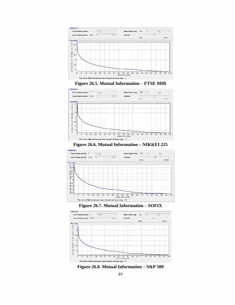
97

Figure 26.5. Mutual Information – FTSE MIB

Figure 26.6. Mutual Information – NIKKEI 225

Figure 26.7. Mutual Information – SOFIX

Figure 26.8. Mutual Information – S&P 500

98

APPENDIX 27

Figure 27.1. False Nearest Neighbors – BET-C (D=1 and D=58)

Figure 27.2. False Nearest Neighbors – BUX (D=1 and D=37)

Figure 27.3. False Nearest Neighbors – DAX (D=1 and D=46)

99

Figure 27.4. False Nearest Neighbors – FTSE 100 (D=1 and D=38)

Figure 27.5. False Nearest Neighbors – FTSE MIB (D=1 and D=31)

Figure 27.6. False Nearest Neighbors – NIKKEI (D=1 and D=33)

100

Figure 27.7. False Nearest Neighbors – SOFIX (D=1 and D=39)

Figure 27.8. False Nearest Neighbors – S&P 500 (D=1 and D=62)

101

APPENDIX 28

Figure 28.1. Recurrence Plot – BET-C

M=19 si D=58

Figure 28.2. BET-C evolution

Figure 28.3. Phase Space Plot – BET-C

102

APPENDIX 29

Figura nr.29.1. Recurrence Plot – BUX

M=8 si D=37

Figure 29.2. BUX evolution

Figure 29.3. Phase Space Plot – BUX

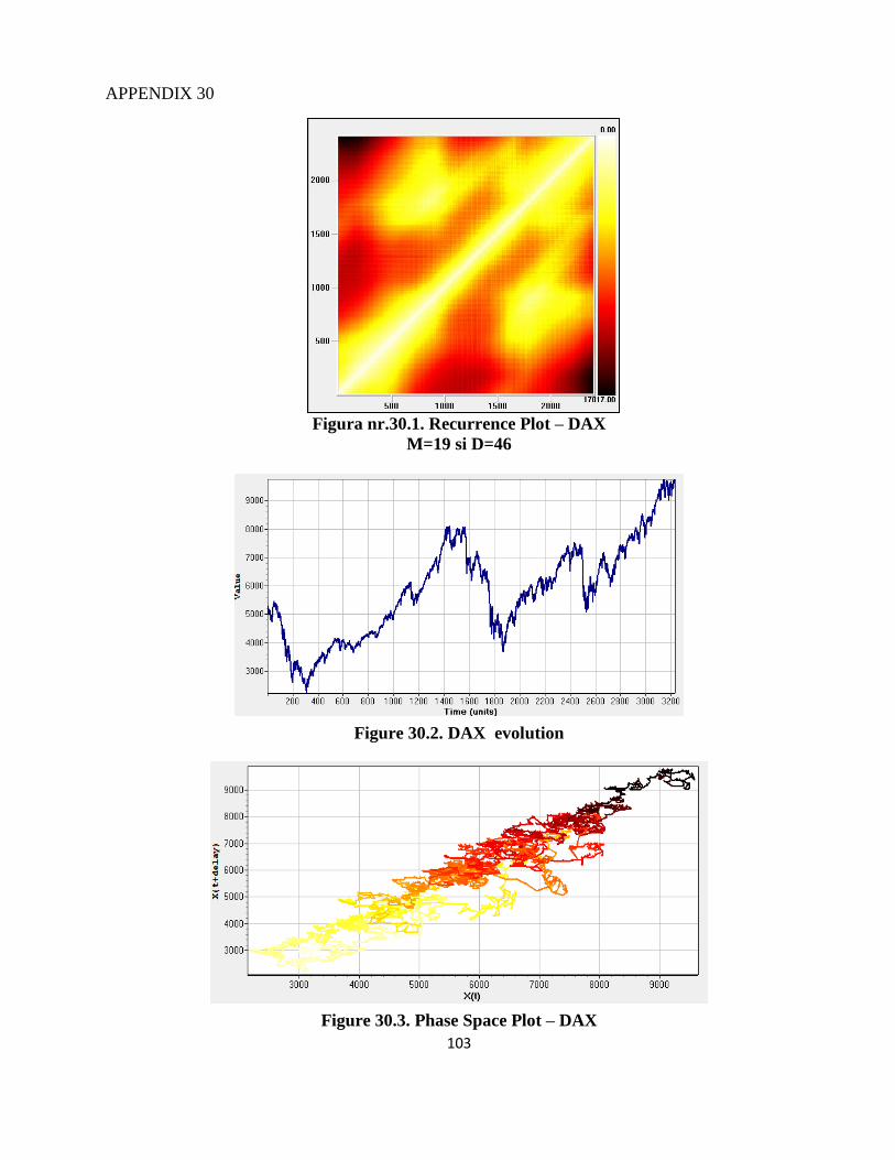
103

APPENDIX 30

Figura nr.30.1. Recurrence Plot – DAX

M=19 si D=46

Figure 30.2. DAX evolution

Figure 30.3. Phase Space Plot – DAX

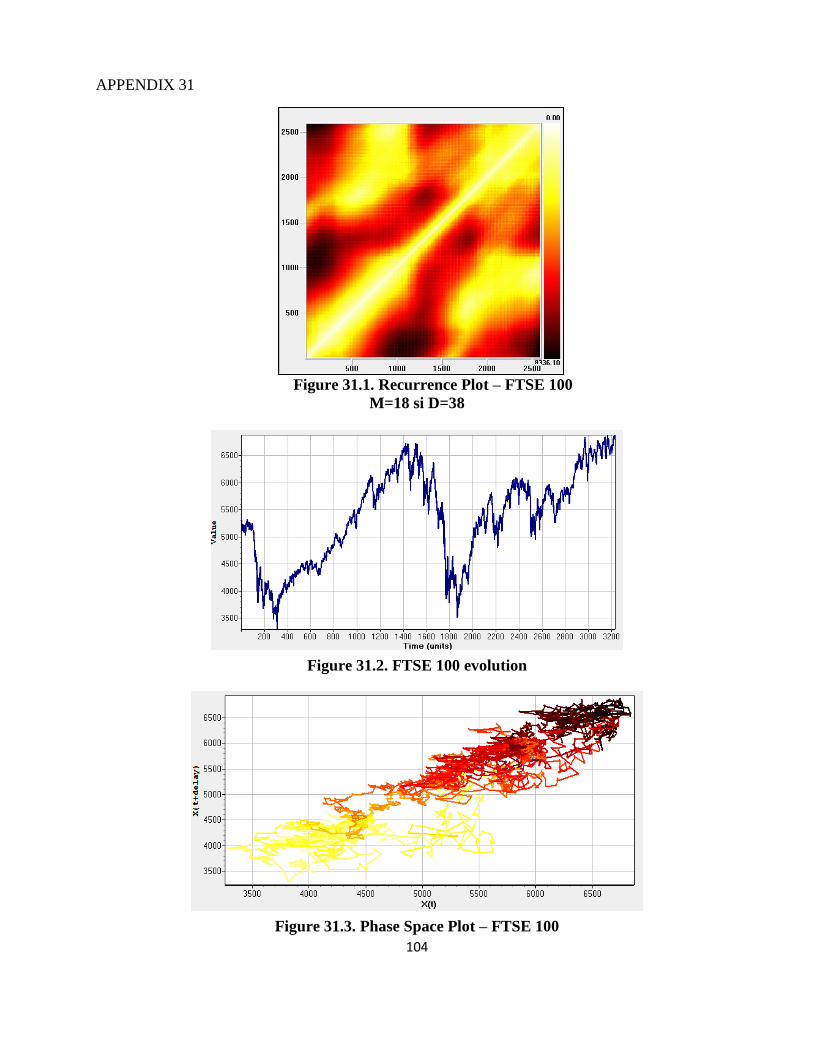
104

APPENDIX 31

Figure 31.1. Recurrence Plot – FTSE 100

M=18 si D=38

Figure 31.2. FTSE 100 evolution

Figure 31.3. Phase Space Plot – FTSE 100

105

APPENDIX 32

Figura nr.32.1. Recurrence Plot – FTSE MIB

M=6 si D=31

Figure 32.2. FTSE MIB evolution

Figure 32.3. Phase Space Plot – FTSE MIB

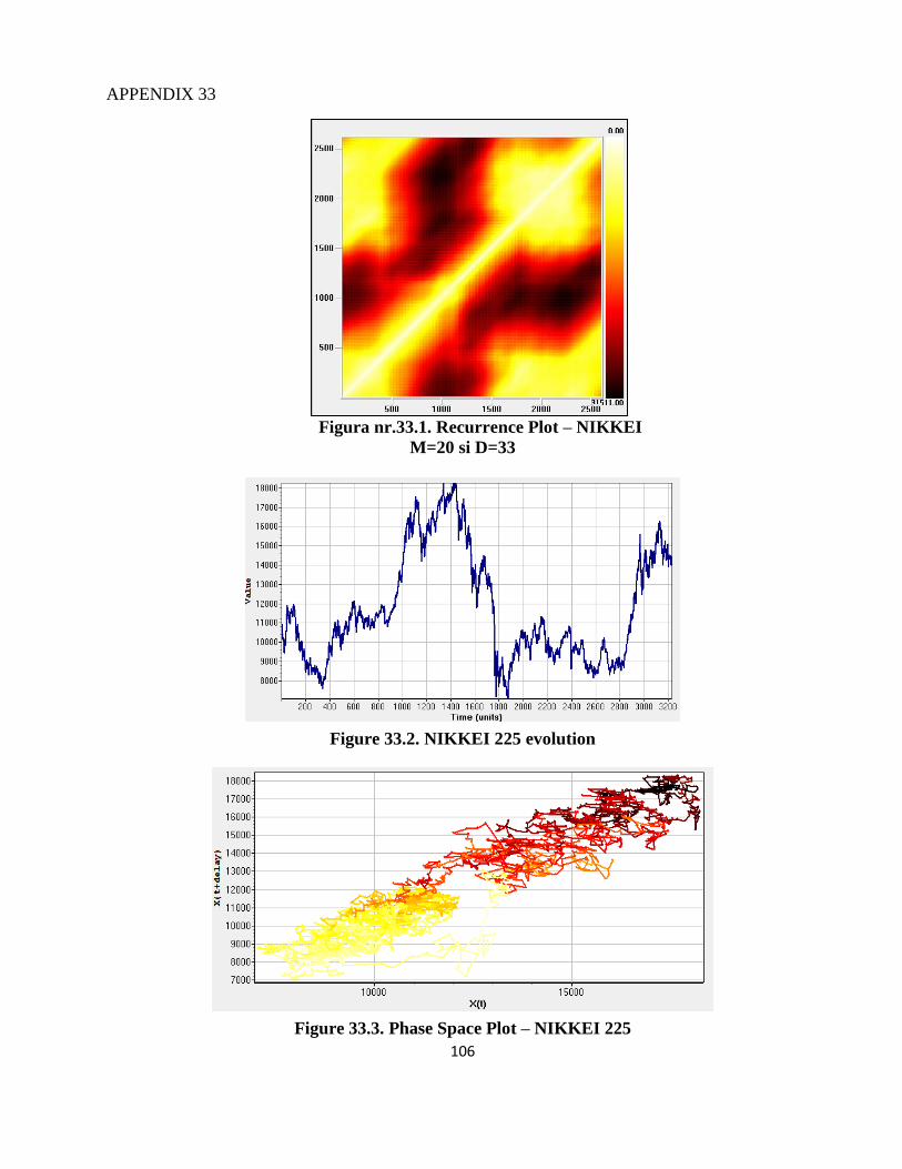
106

APPENDIX 33

Figura nr.33.1. Recurrence Plot – NIKKEI

M=20 si D=33

Figure 33.2. NIKKEI 225 evolution

Figure 33.3. Phase Space Plot – NIKKEI 225

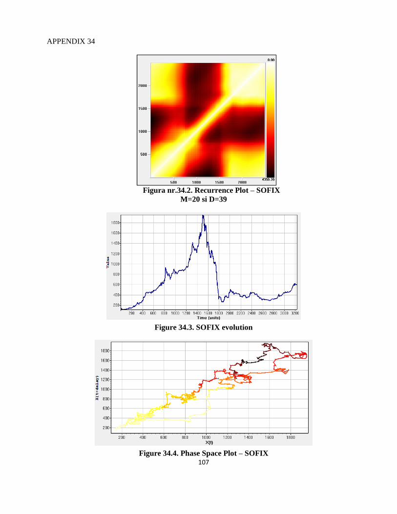
107

APPENDIX 34

Figura nr.34.2. Recurrence Plot – SOFIX

M=20 si D=39

Figure 34.3. SOFIX evolution

Figure 34.4. Phase Space Plot – SOFIX

108

APPENDIX 35

Figura nr.35.2. Recurrence Plot – S&P 500

M=20 si D=62

Figure 35.3. S&P 500 evolution

Figure 35.4. Phase Space Plot – S&P 500

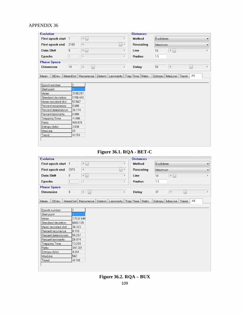
109

APPENDIX 36

Figure 36.1. RQA - BET-C

Figure 36.2. RQA – BUX

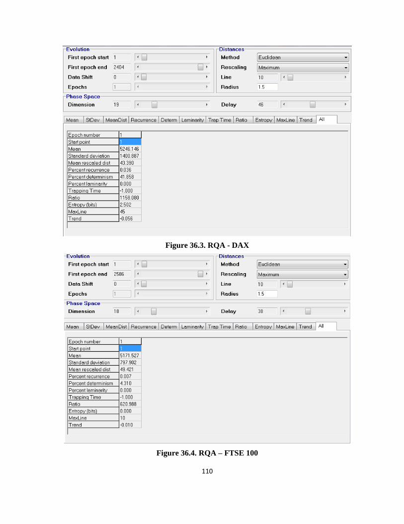
110

Figure 36.3. RQA - DAX

Figure 36.4. RQA – FTSE 100

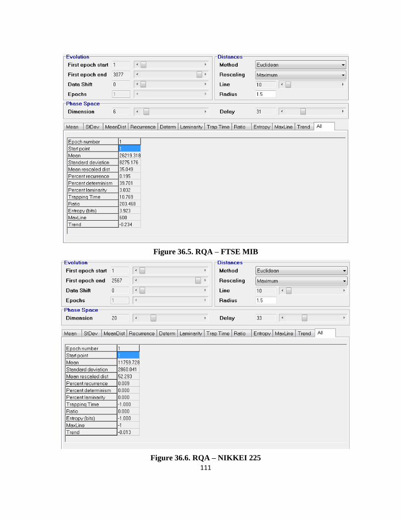
111

Figure 36.5. RQA – FTSE MIB

Figure 36.6. RQA – NIKKEI 225

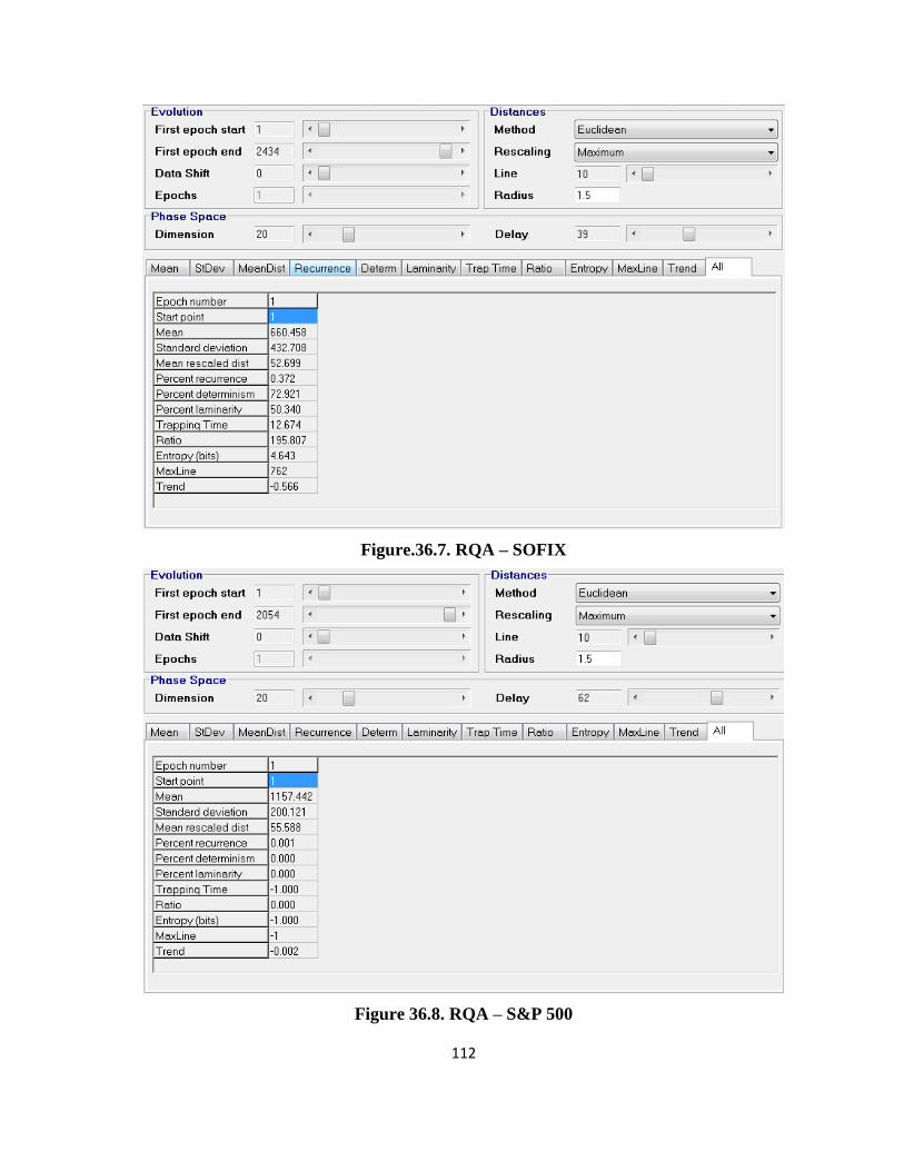
112

Figure.36.7. RQA – SOFIX

Figure 36.8. RQA – S&P 500

113

APPENDIX 37

Figure 37.1. Prediction - BET-C

Figure 37.2. Prediction – BUX

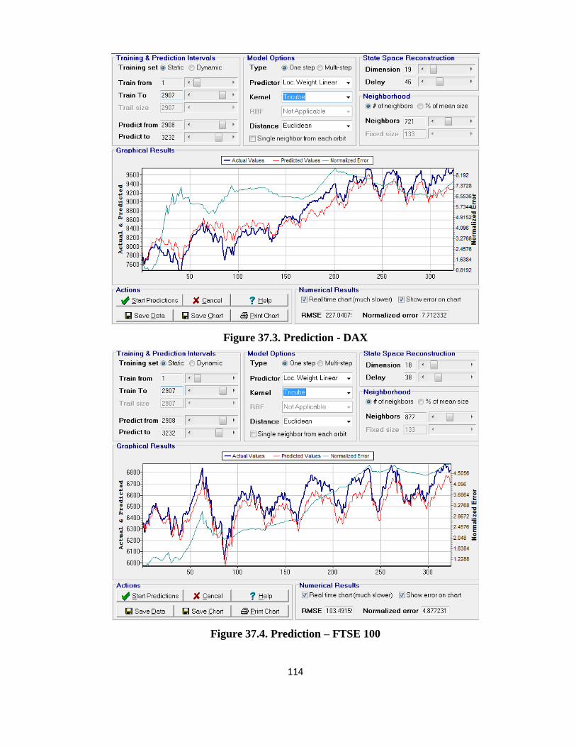
114

Figure 37.3. Prediction - DAX

Figure 37.4. Prediction – FTSE 100

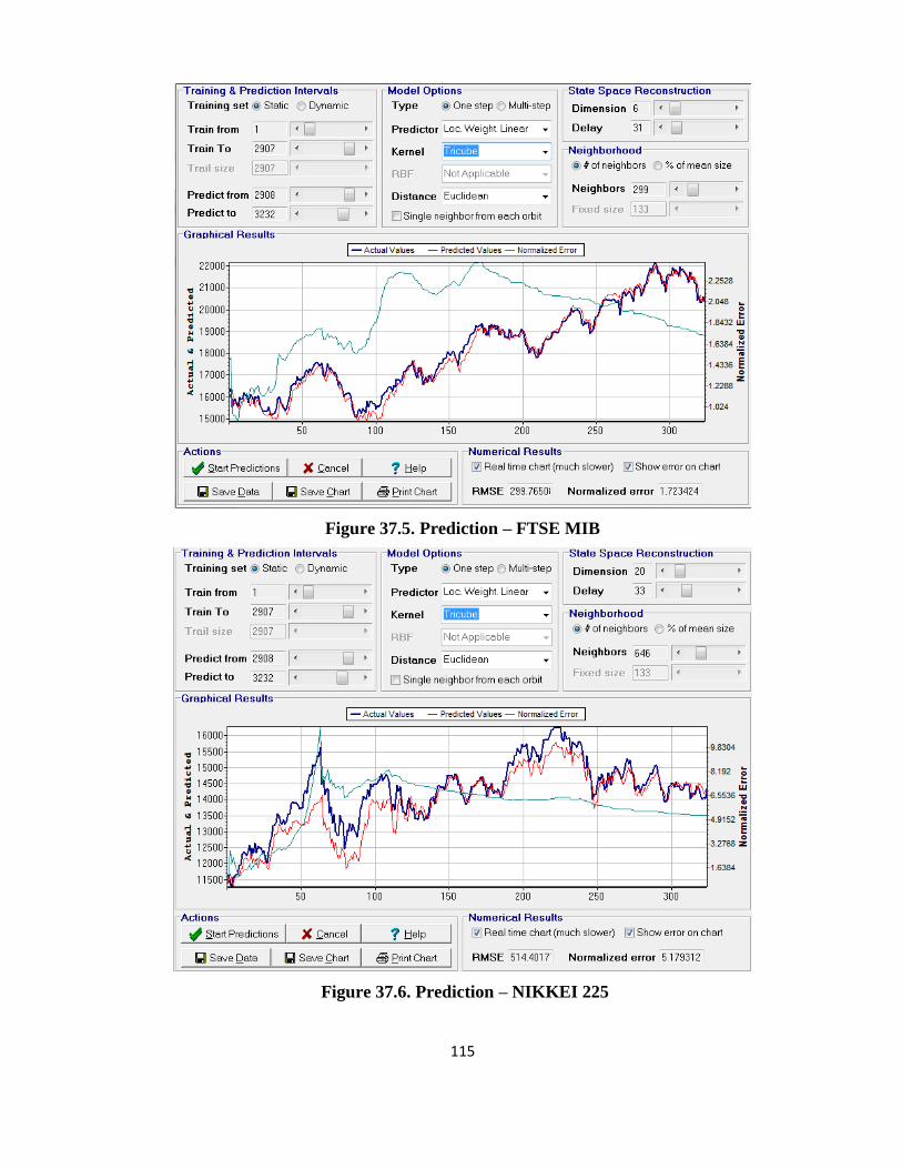
115

Figure 37.5. Prediction – FTSE MIB

Figure 37.6. Prediction – NIKKEI 225

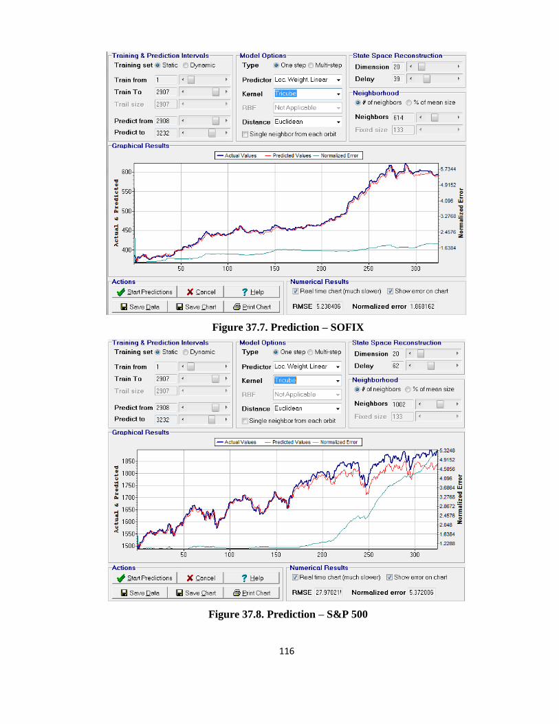
116

Figure 37.7. Prediction – SOFIX

Figure 37.8. Prediction – S&P 500

dissertation paper - finsys.rau.rofinsys.rau.ro/docs/15-msc-rebedia.pdf · complex nonlinear...

Documents