DISSERTATION

SYSTEM ENGINEERING FOR RADIO FREQUENCY COMMUNICATION

CONSOLIDATION WITH PARABOLIC ANTENNA STACKING

Submitted by

Clive Sugama

Department of Systems Engineering

In partial fulfillment of the requirements

For the Degree of Doctor of Philosophy

Colorado State University

Fort Collins, Colorado

Fall 2020

Doctoral Committee:

Advisor: V. Chandrasekar

Anura P. Jayasumana Thomas H. Bradley Jose L. Chavez

Copyright by Clive P. Sugama 2020

All Rights Reserved

ii

ABSTRACT

SYSTEM ENGINEERING FOR RADIO FREQUENCY COMMUNICATION

CONSOLIDATION WITH PARABOLIC ANTENNA STACKING

This dissertation implements System Engineering (SE) practices while utilizing Model

Based System Engineering (MBSE) methods through software applications for the design and

development of a parabolic stacked antenna. Parabolic antenna stacking provides communication

system consolidation by having multiple antennas on a single pedestal which reduces the number

of U.S. Navy shipboard topside antennas. The dissertation begins with defining early phase system

lifecycle processes and the correlation of these early processes to activities performed when the

system is being developed. Performing SE practices with the assistance of MBSE, Agile, Lean

methodologies and SE / engineering software applications reduces the likelihood of system failure,

rework, schedule delays, and cost overruns. Using this approach, antenna system consolidation

via parabolic antenna stacking is investigated while applying SE principles and utilizing SE

software applications. SE / engineering software such as IBM Rational Software, Innoslate,

Antenna Magus, ExtendSim, and CST Microwave Studio were used to perform SE activities

denoted in ISO, IEC, and IEEE standards. A method to achieve multi-band capabilities on a single

antenna pedestal in order to reduce the amount of U.S. Navy topside antennas is researched. An

innovative approach of parabolic antenna stacking is presented to reduce the amount of antennas

that take up physical space on shipboard platforms. Process simulation is presented to provide an

approach to improve predicting delay times for operational availability measures and to identify

process improvements through lean methodologies. Finally, this work concludes with a summary

and suggestions for future work.

iii

ACKNOWLEDGEMENTS

I would like to express my gratitude to my advisor Dr. V. Chandrasekar for the continuous

support of my Ph.D study and related research, for his patience, motivation, and immense

knowledge. His guidance helped me in all the time of research and writing of this dissertation. I

could not have imagined having a better advisor and mentor for my Ph.D study. Besides my

advisor, I would like to thank the rest of my dissertation committee: Dr. Anura P. Jayasumana, Dr.

Thomas H. Bradley and Dr. Jose L. Chavez, for their insightful comments and encouragement, but

also for the feedback which incented me to widen my research from various perspectives. Last but

not the least, I would like to thank my friends and family for supporting me throughout writing

this dissertation and throughout my life.

iv

TABLE OF CONTENTS

ABSTRACT .................................................................................................................................................. ii

ACKNOWLEDGEMENTS ......................................................................................................................... iii

LIST OF TABLES ....................................................................................................................................... vi

LIST OF FIGURES .................................................................................................................................... vii

1. Introduction ............................................................................................................................. 1

1.1. Problem Statement ........................................................................................................................ 4

1.2. Research Objectives ...................................................................................................................... 6

1.3. Dissertation Overview................................................................................................................... 9

2. Background ............................................................................................................................ 12

2.1 Prior RF System Consolidation Efforts....................................................................................... 12

2.2 RF Communication Capabilities Analysis .................................................................................. 14

2.3 Communications for LoS and SATCOM Antennas .................................................................... 16

3. Early Phase System Engineering ........................................................................................... 23

3.1 Interfacing with Planning and Architecture ................................................................................ 28

3.2 Project Planning and Concept of Operations Development ........................................................ 40

3.3 Requirements Engineering .......................................................................................................... 72

3.4 Concept Exploration and Benefits Analysis Phase ..................................................................... 84

4. Antenna Consolidation via Parabolic Antenna Stacking Synthesis ...................................... 94

4.1 Cassegrain with Gregorian Parabolic Stacked Antenna ............................................................ 104

4.2 Gregorian with Splash Plate Antenna ....................................................................................... 113

4.3 Dual Gregorian Parabolic Stacked Antenna ............................................................................. 121

4.4 Dual Cassegrain with Splash Plate Parabolic Stacked Antenna ............................................... 127

4.5 Triple Cassegrain Parabolic Stacked Antenna .......................................................................... 135

4.6 Dual Splash Plate Parabolic Stacked Antenna Assessment ...................................................... 146

4.7 Parabolic Stacked Antenna Configuration Comparison ........................................................... 161

4.8 Technology Maturation and Risk Reduction ............................................................................ 167

5. Mid to Late Phase System Engineering ............................................................................... 175

5.1 Design for Reliability, Availability, and Maintainability ......................................................... 177

5.2 Testing Process Analysis .......................................................................................................... 179

5.3 Production, Deployment, Operations and Support ................................................................... 188

v

6. Summary .............................................................................................................................. 195

6.1 Future Work .............................................................................................................................. 199

References ................................................................................................................................... 201

vi

LIST OF TABLES

Table 1 Antennas with Manufacturers .......................................................................................................... 6

Table 2 SATCOM Capabilities ................................................................................................................... 17

Table 3 CBSP and NMT Frequency Band Capabilities .............................................................................. 18

Table 4 Cubic Sharklink SDT LoS Antenna Capabilities ........................................................................... 22

Table 5 Agile Manifesto [60] ...................................................................................................................... 47

Table 6 Approximate Life Cycle Costs for the Parabolic Stacked Antenna System .................................. 63

Table 7 Annual RDT&E Costs for the NMT System (after [69]) ............................................................... 65

Table 8 Annual Procurement Costs for the NMT System (after [69]) ........................................................ 67

Table 9 Annual Operation and Sustainment Cost for the NMT System (after [69]) .................................. 68

Table 10 Approximate Life Cycle Costs for the NMT System (after [69]) ................................................ 69

Table 11 Annual Operation and Sustainment Costs for the NMT and CBSP Systems with Incremental

Fielding (after [69]) ..................................................................................................................................... 71

Table 12 RF Antenna Standards Profile [20] .............................................................................................. 75

Table 13 Security Features and Functions .................................................................................................. 79

Table 14 Security Quality Attributes .......................................................................................................... 83

Table 15 Pugh Matrix for Antenna Design Concept Selection ................................................................... 87

Table 16 Parabolic Stacked Antenna Service Taxonomy ........................................................................... 91

Table 17 Physical Parameters of the Cassegrain Antenna of the Parabolic Stacked Antenna .................. 108

Table 18 Physical Parameters of the Gregorian Antenna of the Parabolic Stacked Antenna ................... 109

Table 19 Physical Parameters of the Gregorian Antenna of the Parabolic Stacked Antenna ................... 116

Table 20 Physical Parameters of the Splash Plate Antenna of the Parabolic Stacked Antenna ................ 116

Table 21 Dual Gregorian Parabolic Stacked Antenna Physical Parameters ............................................. 122

Table 22 Large and Medium Cassegrain Antenna Physical Parameters ................................................... 129

Table 23 Small Splash Plate Antenna Physical Parameters ...................................................................... 129

Table 24 Triple Cassegrain Parabolic Stacked Antenna Physical Parameters .......................................... 136

Table 25 Physical Dimensions of the Dual Splash Plate Parabolic Stacked Antenna .............................. 148

Table 26 Frequency to Parabolic Stacked Antenna Gain Relationship .................................................... 149

Table 27 Parabolic Stacked Antenna Configurations with Three Antennas ............................................. 163

Table 28 Parabolic Stacked Antenna Configurations with Two Antennas ............................................... 165

vii

LIST OF FIGURES

Figure 1 Shipboard Antennas [14] ................................................................................................................ 5

Figure 2 RF Communication Frequency Bands [25] .................................................................................. 15

Figure 3 SE V Model with DAS (after [47] , [67] ) .................................................................................... 26

Figure 4 Parabolic Stacked Antenna System Architecture ......................................................................... 32

Figure 5 Behavioral Model of the Parabolic Stacked Antenna Sequence Diagram .................................... 33

Figure 6 Consolidated Antenna Reference Sequence Diagram .................................................................. 35

Figure 7 GBS SATCOM Video Transmission OV-1 Diagram .................................................................. 36

Figure 8 Consolidated Video Transmission Sequence Diagram ................................................................. 37

Figure 9 SHF Parabolic Stacked Antenna OV-1......................................................................................... 38

Figure 10 SHF Parabolic Stacked Antenna Sequence Diagram ................................................................. 39

Figure 11 OV-1 Parabolic Stacked Antenna Configuration on U.S. Navy Carrier (after [51]) .................. 41

Figure 12 Materiel Solution Analysis Schedule ......................................................................................... 43

Figure 13 Technology Maturation & Risk Reduction Schedule ................................................................. 44

Figure 14 Engineering and Manufacturing Deployment Schedule ............................................................. 46

Figure 15 Agile Approaches [60]................................................................................................................ 49

Figure 16 Kanban Board Example [61] ...................................................................................................... 50

Figure 17 Scrum Sprint Cycle (after [64]) .................................................................................................. 52

Figure 18 Hybrid Program [67] .................................................................................................................. 56

Figure 19 Models and Learning Cycles (after [68]) .................................................................................... 58

Figure 20 DAS Process WRT Agile Methodologies [59] ........................................................................... 59

Figure 21 Production and Deployment Schedule........................................................................................ 61

Figure 22 Rational DOORS Next Generation Requirements Management Tool ....................................... 74

Figure 23 Requirements Definition and Management Process [75] ........................................................... 76

Figure 24 Security Structural Diagram ....................................................................................................... 80

Figure 25 Security Behavior Model ............................................................................................................ 81

Figure 26 Parabolic Stacked Antenna Layered Service Architecture ......................................................... 90

Figure 27 FMV Distribution Service Context Diagram .............................................................................. 92

Figure 28 Physical Dimensions of a Cassegrain Antenna [79] ................................................................... 95

Figure 29 Cassegrain Antenna Ray Collimation after [80] ......................................................................... 96

Figure 30 Physical Dimensions of a Gregorian Antenna [81] .................................................................... 97

Figure 31 Gregorian Antenna Ray Collimation [82] .................................................................................. 98

Figure 32 PTFE Dielectric Strength at Various Temperatures [89]............................................................ 99

Figure 33 Splash Plate Antenna Ray Collimation [10] ............................................................................. 100

Figure 34 Physical Dimensions of a Splash Plate Antenna [91] ............................................................... 101

Figure 35 Cassegrain and Gregorian Parabolic Stacked Antenna Geometric Properties .......................... 105

Figure 36 Side view of the Cassegrain and Gregorian parabolic stacked antenna ................................... 108

Figure 37 Cassegrain and Gregorian VSWR Values. (a) C band (5.85 GHz to 6.425 GHz). (b) X band

(7.25 GHz to 7.75 GHz). (c) X band (7.9 GHz to 8.4 GHz). (d) Ku band (10.95 GHz to 12.75 GHz). (e)

Ku band (13.75 GHz to 14.5 GHz). (f) Ku band (14.4 GHz to 15.35 GHz. (g) K band (20.2 GHz to 21.2

GHz). (h) Ka band (29 GHz to 31 GHz). (i) Q band (43.5 GHz to 45.5 GHz) ......................................... 110

viii

Figure 38 Radiation Pattern for the Cassegrain and Gregorian Parabolic Stacked Antenna. (a) C band

(6.14 GHz). (b) X band (7.5 GHz). (c) X band (8.15 GHz). (d) Ku band (11.9 GHz). (e) Ku band (14.1

GHz). (f) Ku band (14.875 GHz). (g) K band (20.7 GHz). (h) Ka band (30 GHz). (i) Q band (44.5 GHz)

.................................................................................................................................................................. 112

Figure 39 Gregorian and Splash Plate Stacked Antenna Geometric Properties ....................................... 113

Figure 40 Gregorian and Splash Plate Parabolic Stacked Antenna. (a) Side View. (b) Top View ........... 115

Figure 41 Gregorian and Splash Plate VSWR Values. (a) C band (5.85 GHz to 6.425 GHz). (b) X band

(7.25 GHz to 7.75 GHz). (c) X band (7.9 GHz to 8.4 GHz). (d) Ku band (10.95 GHz to 12.75 GHz). (e)

Ku band (13.75 GHz to 14.5 GHz). (f) Ku band (14.4 GHz to 15.35 GHz). (g) K band (20.2 GHz to 21.2

GHz). (h) Ka band (29 GHz to 31 GHz). (i) Q band (43.5 GHz to 45.5 GHz) ......................................... 118

Figure 42 Radiation Pattern for the Gregorian and Splash Plate Parabolic Stacked Antenna. (a) C band

(6.14 GHz). (b) X band (7.5 GHz). (c) X band (8.15 GHz). (d) Ku band (11.9 GHz). (e) Ku band (14.1

GHz). (f) Ku band (14.875 GHz). (g) K band (20.7 GHz). (h) Ka band (30 GHz). (i) Q band (44.5 GHz)

.................................................................................................................................................................. 120

Figure 43 Dual Gregorian Parabolic Stacked Antenna. (a) Side View [101]. (b) Top View .................... 121

Figure 44 VSWR of the Gregorian Parabolic Stacked Antenna. (a) X band (7.25 GHz – 7.75 GHz). (b) X

band (7.9 GHz – 8.4 GHz). (c) K band (20.2 GHz – 21.2 GHz). (d) Ka band (29 GHz – 31 GHz). (e) Q

band (43.5 – 45.5 GHz) ............................................................................................................................. 123

Figure 45 Radiation patterns of the Gregorian parabolic stacked antenna. (a) X band (7.5 GHz). (b) X

band (8.15 GHz). (c) K band (20.7 GHz). (d) Ka band (30 GHz). (e) Q band (44.5 GHz) ...................... 124

Figure 46 VSWR of the Gregorian parabolic stacked antenna. (a) C band (5.8 GHz – 6.5 GHz). (b) Ku

band (10.8 GHz – 12.8 GHz). (c) Ku band (13.75 GHz – 14.5 GHz). (d) Ku band (14.4 GHz – 15.35

GHz) .......................................................................................................................................................... 125

Figure 47 Radiation patterns of the Gregorian parabolic stacked antenna. (a) C band (6.14 GHz). (b) Ku

band (11.9 GHz). (c) Ku band (14.1 GHz). (d) Ku band (14.875 GHz) ................................................... 126

Figure 48 Dual Cassegrain with Splash Plate Parabolic Stacked Antenna (a) Side view (b) Top view [103]

.................................................................................................................................................................. 128

Figure 49 VSWR of the Dual Cassegrain and Splash Plate Parabolic Stacked Antenna. (a) X band (7.25

GHz - 7.75 GHz). (b) X band (7.9 GHz - 8.4 GHz). (c) K band (20.2 GHz to 21.2 GHz). (d) Ka band (29

GHz - 31 GHz). (e) Q band (43.5 GHz – 45.5 GHz) [103] ...................................................................... 131

Figure 50 Radiation pattern of the Dual Cassegrain and Splash Plate Parabolic Stacked Antenna. (a) X

band (7.5 GHz). (b) X band (8.15 GHz). (c) K band (20.7 GHz). (d) Ka band (30 GHz). (e) Q band (44.5

GHz) [103] ................................................................................................................................................ 132

Figure 51 VSWR of the dual Cassegrain and splash plate parabolic stacked antenna. (a) C band (5.85

GHz to 6.425 GHz). (b) Ku band (10.95 GHz to 12.75 GHz). (c) Ku band (13.75 GHz to 14.5 GHz). (d)

Ku band (14.4 GHz to 15.35 GHz) ........................................................................................................... 133

Figure 52 Radiation pattern of the dual Cassegrain and splash plate parabolic stacked antenna. (a) C band

(6.14 GHz). (b) Ku band (11.9 GHz). (c) Ku band (14.1 GHz). (d) Ku band (14.875 GHz) ................... 134

Figure 53 Triple Cassegrain Parabolic Stacked Antenna. (a) Side view. (b) Top view [104] .................. 136

Figure 54 VSWR of Triple Cassegrain Parabolic Stacked Antenna. (a) X band (7.25 GHz – 7.75 GHz).

(b) X band (7.9 GHz – 8.4 GHz). (c) Ku band (14.4 GHz – 15.35 GHz). (d) K band (20.2 GHz – 21.2

GHz). (e) Ka band (29 GHz to 31 GHz). (f) Q band (33 GHz – 50 GHz). [104] ..................................... 138

ix

Figure 55 Radiation Patterns of Triple Cassegrain Parabolic Stacked Antenna. (a) X band (7.5 GHz). (b)

X band (8.15 GHz). (c) Ku band (14.875 GHz). (d) K band (20.7 GHz). (e) Ka band (30 GHz). (f) Q band

(44.5 GHz). [104] ...................................................................................................................................... 139

Figure 56 Large Cassegrain C Band VSWR and Radiation Details of the Triple Cassegrain Parabolic

Stacked Antenna Configuration ................................................................................................................ 140

Figure 57 Large Cassegrain Ku band VSWR and Radiation Details of the Triple Cassegrain Parabolic

Stacked Antenna Configuration ................................................................................................................ 141

Figure 58 Ku band 13.75 GHz to 14.5 GHz VSWR and Radiation Details of the Triple Cassegrain

Parabolic Stacked Antenna Configuration Comparison. (a) Large Cassegrain Antenna Results. (b)

Medium Cassegrain Antenna Results ....................................................................................................... 142

Figure 59 Ku band 14.4 GHz to 15.4 GHz VSWR and Radiation Details of the Triple Cassegrain

Parabolic Stacked Antenna Configuration Comparison. (a) Large Cassegrain Antenna Results. (b)

Medium Cassegrain Antenna Results. ...................................................................................................... 143

Figure 60 Ka band 29 GHz to 31 GHz VSWR and Radiation Details of the Triple Cassegrain Parabolic

Stacked Antenna Configuration Comparison. (a) Medium Cassegrain Antenna Results. (b) Small

Cassegrain Antenna Results ...................................................................................................................... 144

Figure 61 Q band 43.5 GHz to 44.5 GHz VSWR and Radiation Details of the Triple Cassegrain Parabolic

Stacked Antenna Configuration Comparison. (a) Medium Cassegrain Antenna Results. (b) Small

Cassegrain Antenna Results ...................................................................................................................... 145

Figure 62 Dual Splash Plate Parabolic Stacked Antenna [105] ................................................................ 146

Figure 63 Side View of the Dual Splash Plate Parabolic Stacked Antenna. (a) Side View. (b) Top View

[105] .......................................................................................................................................................... 147

Figure 64 2.248m Splash Plate VSWR and Radiation Pattern for the L band Frequency 950 MHz to 2050

MHz .......................................................................................................................................................... 150

Figure 65 2.248m Splash Plate VSWR and Radiation Pattern for the C band Frequency 3700 MHz to

4200 MHz ................................................................................................................................................. 151

Figure 66 2.248m Splash Plate VSWR and Radiation Pattern for the C band Frequency 5850 MHz to

6425 MHz ................................................................................................................................................. 152

Figure 67 Splash Plate VSWR and Radiation Pattern for the X band Frequency 7250 MHz to 7750 MHz.

(a) Large Splash Plate Results. (b) Small Splash Plate Results ................................................................ 153

Figure 68 Splash Plate VSWR and Radiation Pattern for the X band Frequency 7900 MHz to 8400 MHz.

(a) Large Splash Plate Results. (b) Small Splash Plate Results. ............................................................... 154

Figure 69 Splash Plate VSWR and Radiation Pattern for the Ku band Frequency 10.95 GHz to 12.75

GHz. (a) Large Splash Plate Results. (b) Small Splash Plate Results ....................................................... 156

Figure 70 Splash Plate VSWR and Radiation Pattern for the Ku band Frequency 13.7 GHz to 14.5 GHz.

(a) Large Splash Plate Results. (b) Small Splash Plate Results ................................................................ 157

Figure 71 Splash Plate VSWR and Radiation Pattern for the Ku band Frequency 14.4 GHz to 15.35 GHz.

(a) Large Splash Plate Results. (b) Small Splash Plate Results ................................................................ 159

Figure 72 810mm Splash Plate VSWR and Radiation Pattern for the K band Frequency 20.2 GHz to 21.2

GHz ........................................................................................................................................................... 159

Figure 73 810mm Splash Plate VSWR and Radiation Pattern for the Ka band Frequency 29 GHz to 31

GHz ........................................................................................................................................................... 160

Figure 74 810mm Splash Plate VSWR and Radiation Pattern for the Q band Frequency 43.5 GHz to 45.5

GHz ........................................................................................................................................................... 161

x

Figure 75 Triple Parabolic Stacked Antenna Configuration Comparison ................................................ 164

Figure 76 Dual Parabolic Stacked Antenna Configuration Comparison .................................................. 166

Figure 77 Risk Matrix ............................................................................................................................... 173

Figure 78 PITCO Testing IDEF0 .............................................................................................................. 181

Figure 79 Simulated PITCO Process ........................................................................................................ 183

Figure 80 Probability Density Function for Triangular Distribution ........................................................ 184

Figure 81 PITCO Process Average Delay Time Values ........................................................................... 185

Figure 82 Simulated Lean PITCO Process ............................................................................................... 186

Figure 83 Lean PITCO Process Average Delay Time Values .................................................................. 187

Figure 84 FFBD WRT System Operation and Maintenance .................................................................... 191

Figure 85 NMT Antenna in Radome Space [69] ...................................................................................... 192

1

1. Introduction

System Engineering (SE) involves the collaboration of various engineering disciplines to

produce a service or product (system). A system contains a life cycle which begins with system

requirements and ends with disposal of the system. Performing SE throughout the system life

cycle is critical in delivering a quality product. Performing SE and planning in the early phases is

especially important to prevent rework, schedule delays, and cost over runs. SE rigor is

recommended to increase the chances of project success in terms of cost, schedule, and overall

performance of a system. Model Based System Engineering (MBSE) is a form of SE that uses

models as a backbone for engineering, and expands on improvements that can be made from a

base lined model or simulation. Producing models can demonstrate current and future states of a

process, concept, or operational view of a system. Molding a more efficient methodology from a

base lined model can create a target (goal) that a team can work towards to accomplish

successfully. Integrated models can show an entire engineering effort, and display potential risk

areas for neighboring systems.

As technology brings forth new capabilities for Satellite Communication (SATCOM) and

Line of Sight (LoS) systems, the need to incorporate these capabilities are desired especially with

our military forces. Various frequency bands are accessed with antennas and satellites to make

use of SATCOM and LoS capabilities. Developing consolidated SATCOM and LoS antenna

systems can be complex, and require performing SE activities early in the system life cycle.

Leveraging SE software applications and practices assist with producing state of the art

consolidated SATCOM and LoS systems.

History has shown the importance of early phase system engineering through lessons

learned. In December of 1982, an antenna was being hoisted on top of a 1,800 foot tower where

2

a lifting mechanism failed. The antenna fell and severed a guy wire, bringing down the tower [1].

Not only did this catastrophe cause an antenna and tower to fall, but it cost the lives of 5 people.

Consideration for lifting this type of antenna during the early phases of the system’s life cycle may

have prevented this tragedy. This particular antenna was unintentionally designed to include the

microwave baskets being in the way of the lifting cables. The placement of the hoisting lugs

allowed the antenna to be lifted horizontally off the delivery truck, but the baskets interfered with

the lifting cables when the antenna was rotated to a vertical position [2]. This led to a separate

hoisting mechanism to be fabricated in order to lift the antenna. The hoisting mechanism failed

which resulted in an unfortunate chain of events. Early phase SE may have prevented this by

identifying requirements for lifting. Requirement elicitation and collaboration among stakeholders

prior to the actual design in regards to hoisting practices could have altered this design to account

for specific lifting practices.

In October 1989 NASA launched a Jupiter bound Galileo space craft to obtain 60,000

photos of the planet. This space craft had high and low gain antennas aboard to relay these photos

back to earth years later. The high gain antenna had been stowed behind a sun shield since

Galileo's launch in October 1989, to avoid heat damage while the spacecraft flew closer to the sun

than the orbit of Earth [3]. NASA officials noticed there was a failure when attempting to deploy

the antenna as the space craft was heading towards Jupiter. Based on information received from

the satellite and studies of a mock-up on Earth, engineers at NASA's Jet Propulsion Laboratory in

Pasadena have concluded that three of the antenna's 18 graphite composite ribs are probably stuck

in the folded position [4]. NASA officials believed that the stuck antenna could have been caused

by a loss of lubrication during the transport of the equipment between Florida and California.

Various engineers worked countless hours to come up with solutions to loosen the stuck antenna

3

remotely. Attempts that included repeatedly having the motor turn on / off, spinning the spacecraft

to its fastest rotation possible, turning the spacecraft sideways towards and away from the sun had

no impact on the stuck antenna. An attempt was made to raise the acceleration around Jupiter to

free the stuck antenna, but was unsuccessful. Utilizing the existing low gain antenna was the only

option where efforts to get the most out this low speed antenna was made. Engineers developed

data compression techniques, modulation efficiencies, intricate coding advancements, and

improved S-Band signal to noise ratio antenna designs from the Galileo dilemma. Despite a failed

high-gain antenna and a fussy tape recorder, more than 70% of the original Galileo Prime Mission

science objectives were accomplished using the low gain antenna [5].

Software applications such as Rational DOORS, Rational Rhapsody, Innoslate,

ExtendSIM, Antenna Magus, and CST Microwave Studio provide engineers tools that decrease

the likelihood of system failure, rework, schedule delays, and cost overruns. These software tools

enhance the development of SATCOM and LoS antenna systems. Utilizing these tools allow

engineers to obtain and deliver information necessary to perform SE practices throughout the

system life cycle. Rational Doors is a leading requirements management tool that makes it easy

to capture, trace, analyze, and manage changes to information [6]. Rational Rhapsody provides a

collaborative design, development and test environment for systems engineers and software

engineers that supports UML, SysML and AUTOSAR [7]. The software Innoslate supports system

engineers throughout the lifecycle by integrating requirements analysis and management,

functional analysis and allocation, solution synthesis, test/evaluation, and simulation [8].

ExtendSIM is a software application for finding operational performance of any system using

discrete event simulation [9]. Antenna Magus is a software tool to help accelerate the antenna

design and modeling process. It increases efficiency by helping the engineer to make a more

4

informed choice of antenna element, providing a good starting design [10]. Systems Engineering

involves breaking a complex problem up into smaller, more manageable pieces [11]. CST

Microwave Studio assists with modeling and simulation of antennas by providing metrics such as

Voltage Standing Wave Ratio (VSWR) and radiation patterns. SE software applications aids in

solving these manageable pieces.

Going through the SE development process allows engineers to prepare for later phases of

the system life cycle. Leveraging SE and engineering software applications assist with document

artifact composition. This dissertation specifies an approach for utilizing software applications

and SE practices that support early phase SE and planning for consolidated SATCOM and LoS

antenna system development.

1.1. Problem Statement

Various Radio Frequency (RF) capabilities are required for the military to meet mission

requirements. The Navy wants to increase Fleet warfighting capability while reducing the number

of single function RF systems required on Navy ships [12]. The need for the consolidation of RF

antennas is vital to reduce cost, size, weight, and power consumption on shipboard platforms. The

topside of Navy ships is crowded and the space available for new antennas, systems and

capabilities is limited by the number of existing topside systems [13]. Figure 1 depicts numerous

individual antennas performing unique functions.

5

Figure 1 Shipboard Antennas [14]

Various antennas are procured to perform specific capabilities for shipboard platforms.

The Navy Multiband Terminal (NMT) manufactured by Raytheon, supports Extremely High

Frequency (EHF) / Advanced EHF Low Data Rate /Medium Data Rate/Extended Data Rate, Super

High Frequency, Military Ka (transmit/receive) and Global Broadcast Service (GBS) (receive-

only) communications [15]. The Harris Commercial Band Satellite Program (CBSP) WSC-6

terminals operate in X and Ka band over DSCS/WGS or allied military satellites and C band over

commercial satellites [16]. The Harris CBSP FLV SATCOM equipment involves 8.9-foot

terminals with C- and Ku-band capabilities [17]. A LoS antenna that is used on shipboard

platforms include Cubic’s Sharklink Surface Data Terminal (SDT) which operates within the Ku

band for directional LoS operations. The Cubic Sharklink SDT uses Common Data Link (CDL),

the DoD intelligence, surveillance, and reconnaissance (ISR) data link standard [18]. The Cubic

6

SDT has a directional antenna along with an omni antenna. This research focuses on consolidating

the directional portion of this type of LoS antenna. Obtaining replacement antenna’s and

components from different manufacturers is costly. Table 1 shows antennas being provided by

different manufacturers to provide various RF features.

Table 1 Antennas with Manufacturers

Manufacturer Nomenclature Frequency Purpose

Raytheon NMT X/Ka, Q/KA EHF,SHF SATCOM

Harris CBSP FLV, ULV, WSC-6 SHF SATCOM

Cubic SDT SHF LoS

Multiple RF systems have individual life cycle costs associated with them which require

specific subject matter expertise to maintain which increase overall costs. This research

documents existing systems for consolidation in order to fulfill the Navy’s need to reduce costs

along with reducing the amount of topside antennas. Having a joint RF system would reduce the

number of antennas needed as well as unearth new enhanced capabilities.

1.2. Research Objectives

This dissertation proposal is focused on synthesizing antenna consolidation under a system

engineering perspective. Performing early phase system engineering practices while considering

system life cycle and cybersecurity criteria is critical on developing requirements for antenna

development. An approach to reduce the number of top side antennas is necessary to minimize

the amount of space consumed by various antennas on U.S. Navy shipboard platforms. Antenna

consolidation synthesis involves research of different kinds of antennas to identify limitations as

well as consider different alternatives to combine antenna capabilities to a single platform. NMT

(Q / Ka, X / Ka), CBSP (FLV, ULV) and directional SDT antenna capabilities are investigated to

7

propose a consolidated solution. Capabilities of these antennas are listed to establish a baseline

for a platform that is able to operate at frequencies these various antennas achieve. Identifying

constraints of antenna consolidation such as antenna type and size assisted with proposed antenna

consolidation techniques. Antenna dish size and type limits the frequency capabilities and strength

of a RF signal. The joint functional area includes integrating CBSP and NMT antennas. This will

combine commercial and military RF band capabilities onto a single antenna pedestal. The range

of military operations include LoS and SATCOM communications to include unclassified and

classified capabilities such as NIPRNet, SIPRNet, voice over IP, and data transfer. Commercial

satellite links are also required to provide quality of life technology access such as internet, email,

chat, voice and data transfer services. The timeframe under consideration consists of approval of

the Materiel Develop Decision NLT 15 years prior to the end of life of the NMT antenna.

The required capability of operating at L, C, X, Ku, K, Ka and Q band frequencies stem

from existing operations that the antenna variants of the NMT, CBSP and SDT systems provide.

Consolidating multiple antenna variants such as the NMT Q / Ka, NMT X / Ka, CBSP ULV, CBSP

FLV and SDT directional antennas onto a single pedestal capable of operating at frequencies

spanning across will reduce the number of antennas required on topside shipboard platforms. This

capability is required to provide LoS and SATCOM links to the warfighter. Mission area

contributions include military unclassified and classified LoS and SATCOM links along with

commercial satellite links. The operational outcome the parabolic stacked antenna provides

includes operating at L, C, X, Ku, K, Ka and Q band frequencies for communication capabilities.

The parabolic stacked antenna would include multiple LoS and SATCOM communication groups

to connect to this antenna for transmit and receive communication link purposes. This parabolic

stacked antenna compliments the warfighting force by integrating multiple antennas that consume

8

topside space onto a single pedestal capable of utilizing the same required frequency bands. To

achieve desired operational outcomes, LoS and SATCOM communication groups would have to

connect to the parabolic stacked antenna with a RF switch mechanism to access particular

frequency bands required. The functions that cannot be performed currently includes a single

pedestal antenna capable of providing communication links on L, C, X, Ku, K, Ka and Q RF bands.

Different variant antennas which include the CBSP FLV, CBSP ULV, NMT Q / Ka, and NMT X

/ Ka antennas are required to support missions that use those particular RF bands for SATCOM

and the directional SDT antenna for LoS operations. Due to the amount of antennas needed to

provide these communication links, smaller shipboard platforms are left without the luxury of

having some of these RF capabilities. Some of these ships may have a couple of antenna variants

aboard that provide limited mission critical capabilities due to the amount of space available

topside for RF antennas. The attributes of the desired capabilities include various operations that

the CBSP, NMT and directional SDT RF system variants provide. These operations include

imagery distribution, NIPRNet, SIPRNet, secure communications, VTC, legacy data transfer, file

transfer services, file delivery, video / audio services, secure communications and protected

communications. Providing these operational services through multiple communication links

provide the war fighter a vast array of capabilities utilizing a multitude of RF bands. Cybersecurity

implementation would have to be considered utilizing directives outlined in the DoDI 8510.01

Risk Management Framework (RMF). The RMF process allow the parabolic stacked antenna

system to go through the required information assurance rigor needed to prevent any potential

vulnerabilities. Potential vulnerabilities include RF signal jamming to shutdown communication

capabilities, outdated virus / malware prevention software on client workstations, outdated

firmware on devices such as firewalls, switches, routers, HAIPE, workstations, and RF equipment,

9

password complexity, minimal access control, lack of device configuration backups, inadequate

redundancy options / plans, and limited encryption on network connected devices [19]. These

vulnerabilities would have to be considered throughout the design of the parabolic antenna system

along with the communication groups that the antenna is connected to.

System engineering relating to the Defense Acquisition System (DAS) process is

investigated to determine methodologies for parabolic antenna system development throughout

the system life cycle. Methodologies to include process analysis is included to determine delay

times of testing antenna equipment and to promote lean methods for process improvement.

Analyzing and planning for process related testing events allow for accurate schedule estimating.

Forecasting delay times also assists with Reliability, Availability, and Maintainability (RAM)

metrics for measuring operational availability. Researching previous efforts and baselining costs

is another research effort to assist with budgeting for overall life cycle costs of the parabolic

stacked antenna. Life cycle costs would include activities within the DAS process with respect to

the System Engineering Vee model, and incorporating Agile methodologies to decrease delivery

times and cost. Use cases are depicted to illustrate various scenarios the parabolic stacked antenna

would provide. An overall approach to develop a parabolic stacked antenna using system

engineering methods is investigated and depicted within this research.

1.3. Dissertation Overview

Section 2 provides a background for the research of antenna consolidation. This section

includes prior RF system consolidation efforts to include efforts by the Office of Naval Research

(ONR) Integrated Topside (InTop) program and the Surface Electronic Warfare Improvement

Program (SEWIP). The NMT antenna was another antenna consolidation effort which combined

10

the EHF, SHF, and GBS antenna on a single pedestal. The CBSP antenna is also discussed which

replaced the AN/WSC-8 C band antenna and integrated additional RF band capabilities. RF

communication capabilities are identified and depicted to provide an overview of the RF spectrum.

SATCOM and LoS capabilities along with NMT, CBSP and directional SDT RF band capabilities

are defined to set a baseline for a consolidated SATCOM antenna.

In section 3, early phase system engineering is discussed to strategize an approach for

developing a consolidated SATCOM antenna. The DAS process along with the SE Vee model is

proposed to provide a process for the development of a parabolic stacked antenna which would

combine NMT, CBSP and directional SDT antenna RF band capabilities. A parabolic stacked

antenna system architecture is presented to depict various interfaces that the parabolic stacked

antenna would be connected to. Various use cases and sequence diagrams for LoS and SATCOM

operation are also illustrated to provide insight on potential mission applications. In addition,

conceptual diagrams such as the parabolic stacked antenna OV-1 show antenna capabilities that

can provide communication links to satellites and LoS operations to other antennas. Project

planning using historical data from prior NMT efforts allowed for schedule and cost forecasts

when developing a parabolic stacked antenna. Agile methodology is examined with the use of SE

practices to reduce development costs and delivery times. Exploring various alternatives using the

Pugh matrix provided a system engineering approach to selecting the parabolic stacked antenna as

a solution. Performing early phase system engineering improves planning for the development of

a parabolic stacked antenna.

Antenna consolidation via parabolic antenna stacking is researched in Section 4. Parabolic

antenna stacking allows multiple antennas to be placed on a single pedestal to achieve multiple RF

11

capabilities. Gregorian, Cassegrain and splash plate parabolic antennas were investigated to

demonstrate multiband capabilities through simulation. Different configurations were proposed

utilizing the parabolic stacking methodology. VSWR, gain values, radiation patterns, angular

width, and side lobe levels were captured for parabolic antenna stacking analysis. Simulations

were based off values captured from NMT, CBSP and directional SDT RF band capabilities shown

in Section 2. Physical descriptions and simulation results of the parabolic stacked antenna

configurations are listed to compare against one another. Risk reduction methods are discussed

based off of identified risks for the parabolic stacked antenna system life cycle.

In Section 5, mid to late phase SE is considered to include planning for parabolic stacked

antenna sustainment efforts. Process analysis is introduced to determine delay times of known

process areas which support operational availability metrics. Simulating a PITCO process using

triangular distribution probability methods demonstrated anticipated delay times to be used for

process improvement. The simulation proved that schedule estimation accuracy is increased by

predicting delays within the process as well as proposing lean methodologies for process

improvement. Utilizing SE models such as a FFBD depicted a high level view for operation and

sustainment activities.

Section 6 concludes with a summary of the research that was completed within this

dissertation. The focus areas of the research objectives are presented and key points are identified.

Future work is also recommended at the end of this section.

12

2. Background

Research was conducted to identify requirements for RF system consolidation. A Systems

Engineering approach was conducted to assess requirements, define functional / physical

characteristics, and provide a conceptual design. RF communication capabilities that are currently

in use were assessed to incorporate within the consolidated RF system architecture. A consolidated

antenna approach was proposed to meet the current and future needs of government and military

entities. RF system standards along with non-functional and functional requirements assist with

RF system design. Various communication links would be achieved by utilizing a single antenna

with different assemblies and sub-assemblies.

Integrating RF communications systems provides the advantage of reducing overall

antenna footprints, life cycle costs, multiple RF system maintenance, logistics support and

procurement costs / lead times associated with acquiring various antenna systems / replacement

parts from different vendors. Maintaining multiple RF antennas involves various Subject Matter

Experts (SME), stakeholders and personnel associated with the system’s program of records [20].

A methodology of RF system consolidation, requirements for design, and process planning

considerations are gained from this research. Mission use cases along with proven feasibility are

achieved for the RF system consolidation effort.

2.1 Prior RF System Consolidation Efforts

Various efforts have been performed to reduce the amount of antennas on U.S. Navy

shipboard platforms. The Surface Electronic Warfare Improvement Program (SEWIP) intended

to upgrade the AN/SLQ-32 system. The AN/SLQ-32 was a radar system that allowed U.S. Navy

ships to defend themselves by detection of various threats. The US Navy’s AN/SLQ-32 ECM

13

(Electronic Countermeasures) system used radar warning receivers, and in some cases active

jamming, as the part of ships’ self-defense system [21]. The SEWIP modernized various aspects

of the AN/SLQ-32 system such as integrating an AN/SSX-1 specific emitter identification

subsystem. Such success of system integration obtained from the SEWIP effort led to the Office

of Naval Research (ONR) Integrated Topside (InTop) program. The ONR InTop program pursued

to consolidate common sets of signal and data processing hardware and apertures. In 2004, the

Advanced Multifunction Radio Frequency Concept used this common set to demonstrate that

radar, electronic warfare, and communications functions could perform simultaneously [22].

NMT is another effort that consolidated various RF systems. EHF and SHF systems along

with a GBS antenna was combined to perform multi-frequency capabilities. This consolidation

reduced the need for three different antennas for the EHF, SHF and GBS systems along with

reducing the EHF and SHF communications racks into one communications rack on shipboard

platforms. The NMT Q / Ka antenna is capable of supporting Q and Ka band frequencies for EHF

and SHF transmit / receive capabilities along with K band frequency reception for GBS

capabilities. The NMT X / Ka antenna is capable of supporting X and Ka band frequencies along

with reception of the K band frequency for GBS capabilities. This consolidation breakthrough

reduced the overall topside space that the three antennas was consuming, life cycle costs for

multiple systems, logistic support costs, power consumption and overall weight on shipboard

platforms.

The CBSP system effort consolidated SATCOM systems as well. The CBSP was a rapid

deployment capability acquisition to expedite replacement of Inmarsat B high speed data channel

and Commercial Wideband SATCOM Program capabilities [23]. In addition, the CBSP antenna

replaced Harris’s AN/WSC-8 C band systems along with including adding other frequency

14

capabilities such as X, Ka, and Ku bands. The CBSP antenna system allowed access to commercial

and military satellite links. This equipment also provides access to military NIPRNET and

SIPRNET data, secure telephones, afloat personal telecommunication, video teleconferencing,

telemedicine and medical imagery, national primary image dissemination, and intelligence

database and tactical imagery [17]. This antenna was capable of providing commercial and

military SATCOM communications. The AN/WSC-6(V)9 SHF terminal installed on guided

missile destroyers enabled the ability to also operate in the commercial C-band with a feed horn

change out [24]. Swapping out feed horns was a CBSP solution to achieve multi-band frequencies

utilizing a single antenna pedestal.

The effort to consolidate SATCOM antenna systems has been successful with prior

endeavors. The NMT and CBSP antenna systems have consolidated five systems of record into

just two systems. Multi-band frequency capable antennas have reduced the amount of space,

weight, power and cost to operate multiple RF systems.

2.2 RF Communication Capabilities Analysis

LoS and SATCOM capabilities provide the advantage of sending and receiving

information from remote locations. Satellites that are currently in orbit would drive the

requirement of what signals are to be used on antennas for connectivity and current LoS

frequencies that are in use would provide requirements for LoS operations. Designing an antenna

that can span across various RF frequencies would save on costs for procuring multiple antenna

systems from different vendors. Different satellites would have unique SATCOM band

capabilities and LoS antennas would require a set frequency range to transmit / receive. This would

require a rotatable antenna which can lock into different satellites or antennas to access various

15

communications links. Frequencies for communication systems span over a broad range as shown

in Figure 2. Each allocated frequency range provides unique capabilities.

Figure 2 RF Communication Frequency Bands [25]

The lower in frequency, the larger the wavelength and, accordingly, the more resistant to

fading and blocking a spectrum band will be [26]. Lower frequencies that are below 1 GHz are

resistant against rain and are more tolerable in an urban / high foliage environment. Although

lower frequencies are highly reliable, can travel farther, and can penetrate through objects, they

have a disadvantage of having a lower bandwidth. Applications that do not require much

bandwidth such as voice would be ideal for the lower frequency range. As frequencies increase,

losses by free space, rain, and obstructions increase. Higher frequencies do have advantages by

allowing applications to transmit and receive at higher data rates at a greater capacity.

16

RF system capabilities that are currently being used have to be considered to design a

consolidated solution. LoS and SATCOM methods of communication are critical for remote

military units / platforms. SATCOM provides transmit and receive services to platforms

worldwide based on the satellite’s location and spot beam while LoS capabilities provide data

transfer between platforms directly.

2.3 Communications for LoS and SATCOM Antennas

There are various satellites that are available that are Government owned as well as

commercially provided. Wideband Global SATCOM (WGS) system provides 4.875 GHz

instantaneous switchable bandwidth, along with 500 MHz of X band and 1 GHz Ka band spectrum

allocated to WGS [27]. Defense Satellite Communications System (DSCS) includes a payload of

six-channel SHF transponder and system single channel transponder (X, cross band) [28]. The

AEHF System is the follow-on to the MILSTAR system, augmenting and improving on the

capabilities of MILSTAR, and expanding the military SATCOM architecture, and has onboard

signal processing along with cross banded EHF/SHF communications capabilities [29]. The

MILSTAR satellite can transmit 75 to 2,400 bps of data over 192 channels in the extremely high

frequency (EHF) range [30]. Commercial satellites provide an alternative to Government owned

satellites by providing additional bandwidth resources. Commercial satellites such as AMC, NSS,

SES, INTELSAT, ASTRA, and INMARSAT have SATCOM resources ranging from L band, Ka

band, Ku band, and C band. Table 2 depicts satellites with their respective frequency band

capabilities. Considering these options assist with determining appropriate mission configuration

settings applicable with the location of the beam coverage.

17

Table 2 SATCOM Capabilities

Satellite Frequency Band Capabilities

WGS X-Band, K-Band, Ka-Band [27]

DSCS SHF, X-Band [28]

AEHF EHF, SHF [29]

MILSTAR EHF [31]

AMC, NSS (Commercial) Ku-Band [30]

SES, INTELSAT (Commercial) C-Band, Ku-Band [28] [32]

ASTRA (Commercial) Ku-Band, Ka-Band [30]

INMARSAT-3 F3 (Commercial) L-Band, C-Band [33]

INMARSAT-5 (Commercial) Ka-Band [34]

The locations of these satellites determine the angle at which the antenna would need to be

pointed to. Since the satellites are at various look angles the SATCOM capabilities would be

linked via frequencies shown in Table 2. These satellites provide spot beams to certain locations

around the world to provide services.

Antennas were assessed for SATCOM capabilities aboard U.S. Navy ships. CBSP and

NMT antennas were identified as the major SATCOM antennas with multiple capabilities already.

The CBSP antenna would have L, C, X, Ku and Ka band capabilities. The NMT antenna would

have X, K, Ka and Q band capabilities. Consolidating these antennas would eliminate the need

for buying different antennas from different manufacturers. The CBSP and NMT frequency band

capabilities are shown in Table 3.

18

Table 3 CBSP and NMT Frequency Band Capabilities

Frequency MHz / GHz

Transmit / Receive Antenna Band

7.25 to 7.75 GHz Receive CBSP ULV [35] X

7.9 to 8.4 GHz Transmit CBSP ULV [35] X

10.95 to 12.75 GHz Receive

CBSP ULV [35] Ku

13.75 to 14.5 GHz Transmit CBSP ULV [35] Ku

29 to 31 GHz Transmit CBSP ULV [35] Ka

3.7 to 4.2 GHz Receive CBSP FLV [36] C

5.85 to 6.425 GHz Transmit CBSP FLV [36] C

10.95 to 12.75 GHz Receive

CBSP FLV [36] Ku

13.75 to 14.5 GHz Transmit CBSP FLV [36] Ku

950 to 2050 MHz Transmit / Receive

CBSP FLV [36] L

20.2 to 21.2 GHz Receive NMT [37] K

30 to 31 GHz Transmit NMT [37] Ka

7.25 to 7.75 GHz Receive NMT [37] X

7.9 to 8.4 GHz Transmit NMT [37] X

43.5 to 44.5 GHz Transmit / Receive

NMT [38] [39] Q

The CBSP FLV antennas provide IESS-601 standard G compliant beam patterns using a

2.74m reflector mounted on a high dynamics three-axis pedestal enclosed within a protective

radome [17]. The CBSP FLV antennas continue to provide legacy operations with L band

frequency capabilities. Most unit level access for frigates, mine countermeasures and coastal

patrol ships accessed commercial Inmarsat satellite service with an Inmarsat terminal that operates

strictly in the L-band portion of the RF spectrum, for nothing more than a 64 to 128 kilobyte per

second (Kbps) data rate [40]. The CBSP FLV variant additionally provides C band and Ku band

19

capabilities to provide access to commercial satellites for transmission and reception of files, web

access, e-mail and voice over IP solutions.

The CBSP ULV antenna is capable of accessing military and commercial satellites

depending on the mission and availability. The CBSP ULV antenna is capable of performing X,

Ku and Ka operations. The X band frequency is intended for links to military satellites, the Ku

band frequency is intended for links to commercial satellites, and the Ka band frequency is

intended for communication links for both military and commercial satellites. Since the

designation in the 1970s of a military satellite communications Ka-band (30-31 GHz uplink, 20.2-

21.2 GHz downlink), these frequencies have held great potential to support US forces and

requirements [41]. The CBSP ULV antenna (1.32 m) variant is smaller than the CBSP FLV

antenna (2.74 m) variant. The CBSP ULV antenna variant is capable of supporting reception of

files, web access, e-mail and voice over IP solutions like the CBSP FLV antenna along with having

capabilities to support military missions with NIPRNet, SIPRNet, secure telecommunications and

imagery service. The CBSP ULV does not support the L band, C band and Ku band frequencies

that the CBSP FLV variant supports.

The NMT shipboard antenna variants consist of a large X / Ka antenna (2.44 m), a small

X / Ka antenna (1.54 m) and a Q / Ka antenna (1.37 m). These antennas are utilized for military

satellite links to provide EHF and SHF communications. In addition to X band, Ka band and Q

band capabilities, these antennas support the reception of the K band frequency. The K band

receive frequency is designated for the GBS capability. GBS is an extension of the Global

Information Grid that provides worldwide, high capacity, one-way transmission of video

(especially from Unmanned Aerial Vehicles), imagery and geospatial intelligence products, and

other high-bandwidth information supporting the nation's command centers and joint combat

20

forces in garrison, in transit, and deployed within global combat zones [42]. The NMT X / Ka and

Q / Ka variants support multiband frequency capabilities and are placed on many military

shipboard platforms.

LoS operations provide direct communication links to nearby entities to include shipboard,

airborne, and ground units. The Common Data Link (CDL) protocol interconnects information

from various intelligence, surveillance, and reconnaissance operations that joint military forces are

involved in. This includes all military branches that provide information relevant to mission

success. Information details can be captured by aircraft and relayed to nearby units such as ship

and ground units to assist with strategic decisions. This integrated connection would also work

other ways such as a ground unit relaying information to a nearby ship vessel or an aircraft. Point

to point communication links allow data transfer to occur without the need for SATCOM. Data

transfer to include voice, video and other intelligence information between the military forces in

the air, on the ground and at sea provides situational awareness with real time data. Being able to

share information expeditiously, promotes successful mission execution.

CDL systems typically consist of omnidirectional antennas and / or directional antennas.

Omnidirectional antennas distribute the RF signal equally around the source. The RF signal would

appear as a donut shape around the conductor. A directional antenna radiates energy in one

direction rather than the omnidirectional antenna that distributes the RF energy in a 360 degree

pattern. A directional antenna provides more gain since the RF energy is focused towards a

particular location. The directional antenna provides support for long range operations whereas

the omnidirectional antenna provides support for operations nearby. Typically automatic

switching between the two antennas occur to adjust to mission needs. This research is focused on

the directional antenna capability of LoS operations.

21

The CDL system is aboard aircraft, ground and shipboard platforms. Aircraft platforms

include both manned and unmanned vessels. Unmanned vessels involve drones which can capture

vital information from potential threats. Ground platforms entail mobile platforms whether it’s

vehicular or equipped on personnel and military stations. Unmanned vehicles are also considered

to equip the CDL system to capture and transmit information. Shipboard platforms would use this

information by connecting with other CDL systems to receive and transmit information.

The Light Airborne Multipurpose System (LAMPS) Hawklink is a high-speed, air-to-

ground, digital data link that transmits reconnaissance and other data from MK III H-60 helicopters

to their host surface ships, such as Arleigh Burke Class destroyers [43]. The AN/SRQ-4 Hawklink

is the shipboard element of a situational awareness system that links the MH-60R helicopter with

surface warships in the area [44]. The AN/SRQ-4 is another antenna that can be consolidated by

parabolic antenna stacking for the directional antenna portion. The omni antenna would be

separate to provide near range communication links. The AN/SRQ-4 system has CDL capabilities

that assists surveillance missions and provides a link between neighboring platforms equipped with

CDL technology. Capabilities include secure data transfer, data link operation, full motion video

distribution, interoperability with CDL family of airborne terminals (fire scout, P-3, and P-8) [45].

Real time data to include imagery, and sensor data is also included to support mission

requirements.

Cubic’s Sharklink Surface Data Terminal (SDT) is a new, high performance surface data

terminal that supports secure, long range, high data rate communications with airborne and

shipboard platforms equipped with a DoD standard Common Data Link (CDL) data terminal [18].

LoS communications and beyond line of sight systems promotes a tactical communications

environment. Cooperative Engagement Capability Data Distribution System CEC (CEC DDS)

22

fuses high quality tracking data from participating sensors and distributes it to all other participants

in a filtered and combined state, using identical algorithms to create a single, common air defense

tactical display ("air picture") [46]. The CEC DDS operations use the C-Band frequency range,

and CDL operations operate within the C and Ku band frequency range. The CDL capable SDT

LoS directional antenna is investigated for consolidation purposes within this research and the

frequency capabilities for this LoS antenna is shown in Table 4.

Table 4 Cubic Sharklink SDT LoS Antenna Capabilities

Frequency MHz / GHz Type Antenna

Frequency Band

14.4 to 15.35 GHz Directional

Sharklink Surface Data Terminal (SDT) Ku

14.4 to 15.35 GHz Omni

Sharklink Surface Data Terminal (SDT) Ku

2.2 to 2.5 GHz Omni

Sharklink Surface Data Terminal (SDT) S

4.4 to 4.99 GHz Omni

Sharklink Surface Data Terminal (SDT) C

23

3. Early Phase System Engineering

In order to develop a new consolidated antenna, a planned System Engineering (SE)

approach is required. Utilizing SE practices along with SE software within the early phases of the

system life cycle increase the chances for success. SE includes many aspects such as technical

planning, customer requirements, design, build / integrate, testing, production, deployment, and

operations / sustainment. During this life cycle, system engineering would be needed to ensure

processes are followed through in the most efficient manner while verifying that requirements are

met. SE also includes SE architectures, modeling, technology assessment, capabilities

engineering, as well as system integration.

Applying MBSE early in the life cycle is important to be able to provide models and

simulations to meet system requirements. During the conceptual design phase, activities relating

to design, analysis, verification and validation can be done using MBSE. Models are produced

during the search for solutions & assessments to display alternative system concepts as well as

assessment & concept trade off studies. Performing MBSE early in the life cycle can reduce the

need to perform rework later on due to unforeseen system constraints. MBSE can support

validation of operational behavior and functional performance during the design refinement &

design validation phase. Visually seeing virtual interactions among system components or other

systems within the environment would determine required interfaces as well as other systems that

may be affected. Performing MBSE early on help provide more accurate cost estimates throughout

the life cycle of the system. Displaying models that show neighboring entities as well as

performance characteristics will help facilitate cost projections down the road. Simulations and

models displaying physical constraints, operational constraints, environmental / operational

factors, system synthesis models and simulations can encompass many areas of the system.

24

Determining quantitative values for these activities will tie into cost estimates to ensure adequate

funding is available for the overall effort. Performing MBSE activities as well as Agile

methodologies early on can help reduce cost, and promote the ability to deliver faster. Displaying

a functional and physical architecture of a system is a start to MBSE where these architectures are

expanded upon from system requirements. Determining any constraints or tradeoffs early in the

life cycle will reduce the need to reassess the system later on in the future. Determining issues

early using MBSE and Agile methodologies will help reduce delays in schedule due to rework,

increase cost projection accuracy, and ensure the system is meeting operational needs.

The CBSP, NMT and directional SDT antennas were researched and explored to identify

current frequency band requirements along with satellite connection points for the CBSP and NMT

antennas in section 2.3. Requirements for this antenna design is provided along with a concept of

operations throughout this research. A high level design with simulation results is also provided

within this research. The objective includes following SE practices to propose a consolidated

antenna capable of utilizing frequencies of CBSP, NMT and SDT antennas. High level

requirements were defined to identify functional and non-functional characteristics of the

consolidated antenna.

Boundaries include designing the antenna itself and including the interconnections of the

systems correlating to various existing antennas. Schedule was estimated to identify major

milestones and a budget was estimated for planning purposes. Assumptions, constraints and risks

was identified to account for details relating to the design of the consolidated antenna. Certain

roles and responsibilities were depicted for budget estimation and resource identification needs for

future development.

25

SE has many different fields where incorporating different domains would allow different

SE approaches to be successful when developing a system. SE standards such as the ISO 15288

provides guidance for SE life cycle processes. The processes listed in the ISO 15288 provide

direction on how to perform SE activities. Not all processes listed creates a one size fits all

solution, but does give a way forward for the system engineer to tailor one’s need to accomplish a

SE objective. The SE V Model is an iterative set of processes that depicts the system’s life cycle

from beginning to end.

DoD instruction 5000.02 defines the operation of the Defense Acquisition System (DAS).

The DAS consists of 5 phases of major activities. This can be cross walked with the SE V model.

The major activities include material solution analysis, technology maturation & risk reduction,

engineering & manufacturing development, production & deployment, and operations & support.

Various decision points are also included such as the Material Development Decision (MDD),

Capability Development Document (CDD), Request for Proposal (RFP), and the Full Rate

Production (FRP) decision. Major reviews would include the Preliminary Design Review (PDR),

Critical Design Review (CDR), and Production Readiness Review (PRR). These reviews assist

with obtaining the status of the current development of the system as well as making any major

decisions on changes relating to the cost, schedule and performance of the system. Major

milestone decisions are labeled A, B, and C and are shown in Figure 3 which depicts the DAS

process aligning to the SE Vee model.

26

The Material Solution Analysis phase is the basis of the Defense Acquisition System

process which sets up the acquisition strategy, goals, and provides an analysis of alternatives.

Initially, the Initial Capabilities Document (ICD) specifies the need to fill a capability gap with a

materiel and / or service solution. The ICD includes a Concept of Operations (CONOPS) summary

that depicts how a system would operate. A high level depiction of the system with high level

requirements describes the objectives of the system. Different use case scenarios would be

presented to demonstrate how the system would function in a particular environment. A

description of operational outcomes with how the capabilities would satisfy those objectives is

required. The required capability and capability gaps would be presented in the ICD. Capability

gaps occur when an existing capability is not sufficient, needing to be replaced or does not exist.

Figure 3 SE V Model with DAS (after [47] , [67] )

27

At times, redundant capabilities may be present creating inefficiencies. The Material Development

Decision is the formal decision made to move forward with the Materiel Solution Analysis phase.

This decision point recognizes the need and / or capability gap. In addition, providing the

necessary resources to staff and fund engineering and programmatic tasking is made. This decision

is made based off of the ICD and any other evidence that demonstrates that the approach would

satisfy the need. The schedule would be discussed to show when the capability can be available

and what can be done in the time being to address the need until the system is fielded.

The Material Solutions Analysis (MSA) phase determines potential solutions for a need.

This need would typically come from a technology gap or a new capability that would benefit

mission requirements. An Analysis of Alternatives (AoA) method assists with solution selection.

Listing potential solutions identifies feasible options to choose based off of the selection criteria.

Comparisons would be made off of the solution being operational effective, cost effective, suitable

and meeting the selection criteria parameters. A preliminary acquisition strategy is included to

identify various contract avenues, sustainment plans, program schedule, risk areas, design

considerations, cost information, resource needs, test strategies and other relevant acquisition

requirements. Avenues for material and service contracts would be identified in the acquisition

strategy. A decision would have to be made to determine what material would have to be procured

whether it is COTS or custom made. Contractor services would have to be considered to

supplement the required expertise to assist with the development of the system. Initial plans for

sustainment would be included in the acquisition strategy to include support and maintenance

concepts which would be linked to the Life Cycle Sustainment Plan (LCSP). These sustainment

details provide insight to design considerations that would be required.

28

Milestone A refers to a decision where stakeholders would have to commit resources

required to develop the intended system. Risks would be identified and mitigated prior to

Milestone A in order to obtain stakeholder concurrence. Certain risks may not be easily mitigated

by Milestone A and stakeholders would have to accept certain risks in order to move forward with

the Technology Maturation & Risk Reduction (TMRR) phase. Justifying the preferred system

solution would have to be discussed during the Milestone A decision review. Various alternatives

that were vetted prior to the review would assist with the justification and to demonstrate the

feasibility of the system. The cost, schedule, performance and risks associated with the planned

system would also be reviewed and agree upon during the Milestone A decision review.

Requirements along with the scope of the work involved to develop the system would provide a

common understanding of the magnitude of the entailed effort. The acquisition strategy would

also be discussed to include contracts for both material and services in order to determine how

effective and efficient the strategy is. Overall the approach, assumptions, acquisition strategies,

technology development requirements, affordability, and risks with mitigation activities would

increase approval to move to the next phase after the Milestone A decision review. Written

determination, market research, affordability analysis, AoA, Draft CDD, core logistics

determination / core logistics and sustaining workloads estimate, economic analysis, SE Plan to be

revised are activities performed by Milestone B.

3.1 Interfacing with Planning and Architecture

Modeling architecture takes place in the early planning stages of the system’s life cycle.

During this planning area, interconnecting links are identified. The interconnecting links would

include other systems or components that interface with the system being developed. For a

consolidated antenna being developed, various interconnecting systems would be identified.

29

These interconnecting systems would have various system owners that would have to be

collaborated with. Obtaining historical architectures would assist with integration activities and

design. System architecture would depict various interfaces and data elements of the system. The

data elements would show various types of information exchanged between the systems. The

architecture assists with defining the system’s scope and identifying requirements. The

architecture identifies the integration opportunities that should be considered and provides a head

start for the systems engineering analysis [47]. If historical architecture artifacts are unavailable,

developing an architecture to depict the system with interfaces connecting to other systems is

recommended.

A system architecture can be achieved from MBSE. MBSE establishing a common

language to communicate better through MBSE software tools are essential. SysML is a visual

modeling language that MBSE SMEs use to develop intricate models. This modeling language

fills the gap between system engineering fields of practice. Having a common language whether

it is system engineering, project management, or MBSE can promote better communication

between team members to accomplish the tasks at hand.

A common language for model based system engineers improves collaboration and

cohesion among team members. SysML standards assist MBSE communities to share information

amongst one another to expand on ideas. Receiving help on a common language such as SysML

is easier than obtaining peer support from a proprietary vendor that developed their own language.

MBSE software tools such as IBM Rational Rhapsody, uses SysML to display robust models for

system engineers. SysML modeling would allow insight into complex diagrams where important

decisions can be made from stakeholders. A common language will reduce the need to translate

different languages when integrating models. A scenario where a software tool uses one language

30

that is not compatible with another can force one software language to be manipulated to cater to

the preferred MBSE tool.

Communication gaps can be filled with having a common language when applying MBSE

practices. Having consistency with a common language and capabilities to address issues when

performing MBSE, can promote a cohesive project team. The team being able to communicate

with each other using a common MBSE language can add value to the overall progress for a MBSE

modeling effort. To be able to clearly communicate with all stakeholders using a common

language will allow team members to be on the same page with decision makers. Not being able

to communicate about a MBSE language can cause confusion and loss of interest amongst

members of a team.

The MBSE primer states there is a need for a “systems language” to avoid the natural

ambiguity of language and to enable specialists involved in the SE effort to communicate outside

of their own group [48]. Common language of MBSE would keep everyone on the team on the

same page. Methodologies, thoughts, decisions, and rationale of the way forward on an MBSE

effort will promote a cohesive team that performs efficiently. Reducing MBSE interpretation

issues can be done by defining MBSE related terminology. A common language would be able to

have decision makers determine unavoidable tradeoffs visually depicted by a MBSE model.

Having a common language is significant to the application of MBSE by reducing interpretation

discrepancies which may lead to rework, improving cohesion with views amongst team members,

and the ability to persuade decision makers to select the most cost effective solution.

The existing architecture includes the SDT, CBSP FLV, CBSP ULV, GBS, NMT Q / Ka,

and NMT X / Ka system variants on U.S. Navy shipboard platforms. Depending on the size of the

ship and the amount of space availability, various configurations exist with different combinations

31

of these CBSP, NMT and SDT variants. Some ships may not have all the antenna variants

available to them and are limited to only a select few that are mission critical. Each antenna variant

would have their own unique communications group which would have its’ own set of operations

they perform. The NMT antenna systems have an ability to connect to the GBS communications

group to receive files, video, audio and other data elements. Communication groups would have

their own RF capability values associated with them. Some communications groups have the same

RF capability values along with the same system operations. Although this provides a redundant

backup to one another, it increases costs with maintaining multiple systems. Combining antenna

variants would reduce the amount of antennas needing to be maintained. A parabolic stacked

antenna solution would eliminate the need for multiple antenna variants and provide the same

SATCOM capability that CBSP FLV, CBSP ULV, NMT Q / Ka, and NMT X / Ka antenna variants

currently provide along with the LoS directional capability that the SDT antenna provides. The

parabolic stacked antenna system architecture is depicted in Figure 4 using existing RF

communication groups.

32

Figure 4 Parabolic Stacked Antenna System Architecture

33

NMT and CBSP variant communication groups have operational capabilities that provide

required data to the warfighter. The NMT and CBSP variants have similar operational capabilities

such as NIPRNet, SIPRNet, secure communications, voice, imagery, and other data transfer

services on the MILSATCOM side. These capabilities are used with both NMT and CBSP variant

antennas which occupies space on the topside of U.S. Navy shipboard platforms. The parabolic

stacked antenna would take the place of currently installed NMT and CBSP antenna variants, and

be capable of interfacing with existing communication groups to provide communication services

to the war fighter.

The reference sequence diagram was created to depict a high-level activity flow between

the operator and the external source. This diagram generalizes the parabolic stacked antenna

system where typical concepts of operations are shown. This sequence diagram includes the

operator requesting desired information from the external source through the operator’s internal

network, COMSEC devices, and parabolic stacked antenna system as shown in Figure 5.

Figure 5 Behavioral Model of the Parabolic Stacked Antenna Sequence Diagram

34

The reference sequence diagram was created to depict a high level activity flow between

the operator and the external source for SATCOM systems. This diagram generalizes the parabolic

stacked antenna system where typical concepts of operations are shown. This use case includes

the operator requesting desired information from the external source through the operator’s

internal network, COMSEC devices, and parabolic stacked antenna system.

The sequence diagram shown in Figure 6 displays the events of transmitting and receiving

data via the parabolic stacked antenna system. The parabolic stacked antenna would have the

capability of utilizing a SATCOM signal. The operator would send and request data while the

internal network would encrypt the data using COMSEC devices and sending the data to the

consolidated antenna system. The parabolic stacked antenna system converts the Internet Protocol

(IP) data into a RF signal via modulation. The RF signal would be encrypted and sent to the distant

end with about 500ms latency. The receive signal is obtained by the consolidated antenna system

around the same latency, decrypted and demodulated prior to converting the signal to the IP format.

The IP traffic would be decrypted and sent to the operator. Latency times are approximations

where weather, bandwidth, configurations, assemblies and the type of applications being used

would alter these values.

35

Figure 6 Consolidated Antenna Reference Sequence Diagram

The GBS capability provides high-speed broadcast of large-volume information products

such as video, imagery, maps and weather data to deployed tactical operations centers and

garrisoned forces worldwide [49]. The land-based platform video distribution source would

transmit the streaming video via the consolidated antenna using the Ka band frequency to the WGS

satellite. A parabolic stacked antenna could also be used on the land-based platform to perform

multiband capabilities. The WGS satellite would forward the streaming video to a shipboard

36

platform using the K band capability of the parabolic stacked antenna configured to receive the

required video depicted in Figure 7.

Figure 7 GBS SATCOM Video Transmission OV-1 Diagram

Interactions among the various entities as well as actions that occur that transform inputs

to outputs independently is shown in Figure 8. This sequence diagram illustrates video streaming

from the source to a distant end via SATCOM. Video feeds are essential when performing a

mission to distribute vital intelligence. Observing the sequence diagram to ensure near real time

video streaming is being conducted is useful for timing and performance analysis. GBS operates

as a one-way broadcast capability supporting timely delivery of video products, unclassified &

classified data for mission support and theater info transfer [50].

37

Figure 8 Consolidated Video Transmission Sequence Diagram

The operator at the distant end would configure the parabolic stacked antenna Ka / Ku

configuration to track, and acquire the signal from the satellite. The parabolic stacked antenna

would acquire the signal to make the connection. Once the connection is made, the parabolic

stacked antenna will receive the streaming video. The video would then be distributed through the

internal network. The video would be in the User Datagram Protocol (UDP) format for one way

reception.

A mission thread was modeled which included a shipboard platform, operations center,

and a mobile communications unit. The shipboard platform requested mobile communications

data in order to assess battleground intelligence in a remote location. This SHF connectivity

between the platforms is shown in Figure 9.

38

Figure 9 SHF Parabolic Stacked Antenna OV-1

The shipboard platform would send a request to the operations center for intelligence data

from a mobile communications unit. The mobile communications unit in this use case is a

temporary base set up at a remote location. The operations center would approve or deny the

request while notifying the mobile communications unit. The mobile communications unit would

acknowledge the request for the data and transmit via SHF back to the operations center. The

operations center would forward the mobile communications data to the shipboard platform.

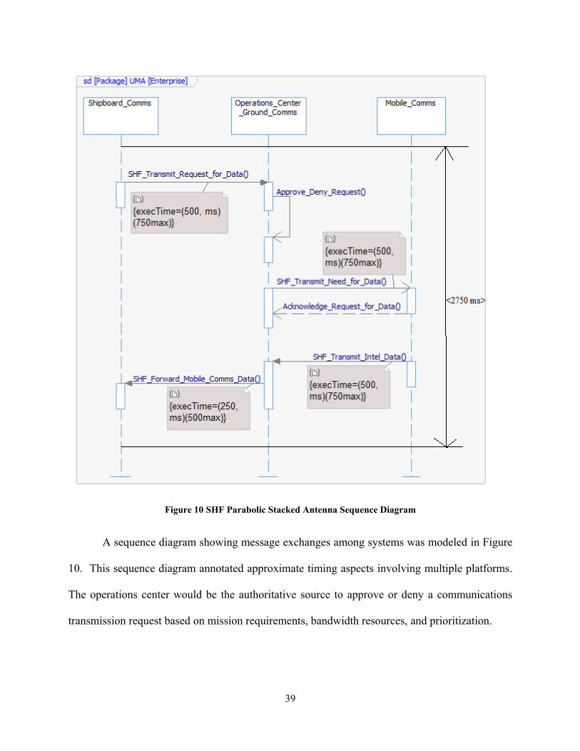
39

Figure 10 SHF Parabolic Stacked Antenna Sequence Diagram

A sequence diagram showing message exchanges among systems was modeled in Figure

10. This sequence diagram annotated approximate timing aspects involving multiple platforms.

The operations center would be the authoritative source to approve or deny a communications

transmission request based on mission requirements, bandwidth resources, and prioritization.

40

3.2 Project Planning and Concept of Operations Development

Project planning is a critical phase where the foundation of guidelines and way forward is

presented on the system being developed. Aspects of cost, schedule, performance, and risks are

identified along with information how the project will be managed. A project management plan

would provide an initial baseline for the expectations of the overall project. A project charter

assists with providing a high level overview of the project along with concurrence to have the

project move forward. A project charter would include elements such as the need, scope, schedule,

cost, stakeholders, roles / responsibilities, assumptions, constraints and risks. This planning phase

artifact would be referenced or incorporated into the project management plan.

The need for antenna consolidation on afloat Navy platforms is ongoing where space is

limited due to the amount of various antennas staged topside. Consolidating these antennas would

free up topside space along with reducing power consumed and the weight that excess antennas

provide. Previous efforts have taken place such as the NMT antenna that consolidated multiple

antennas that supported EHF, SHF, and GBS capabilities. An approach and design for

consolidating existing LoS and SATCOM antennas was researched and an Operational View (OV-

1) is depicted in Figure 11 .

41

Figure 11 OV-1 Parabolic Stacked Antenna Configuration on U.S. Navy Carrier (after [51])

Project planning for the parabolic stacked antenna involves managing the scope of work.

Scope management includes the processes required to ensure the project includes all the work

required, and only the work required, to complete the project successfully [52]. Details of tasks

required and a methodology for change control management assists with progression of

development. A change control process has to be identified early on to address changes in scope.

Any change in scope, whether it’s adding, removing, or changing requirements have to be

documented and agreed upon amongst stakeholders. Without a change control process, the scope

of any effort could potentially be derailed. Scope creep occurs during a project where requirements

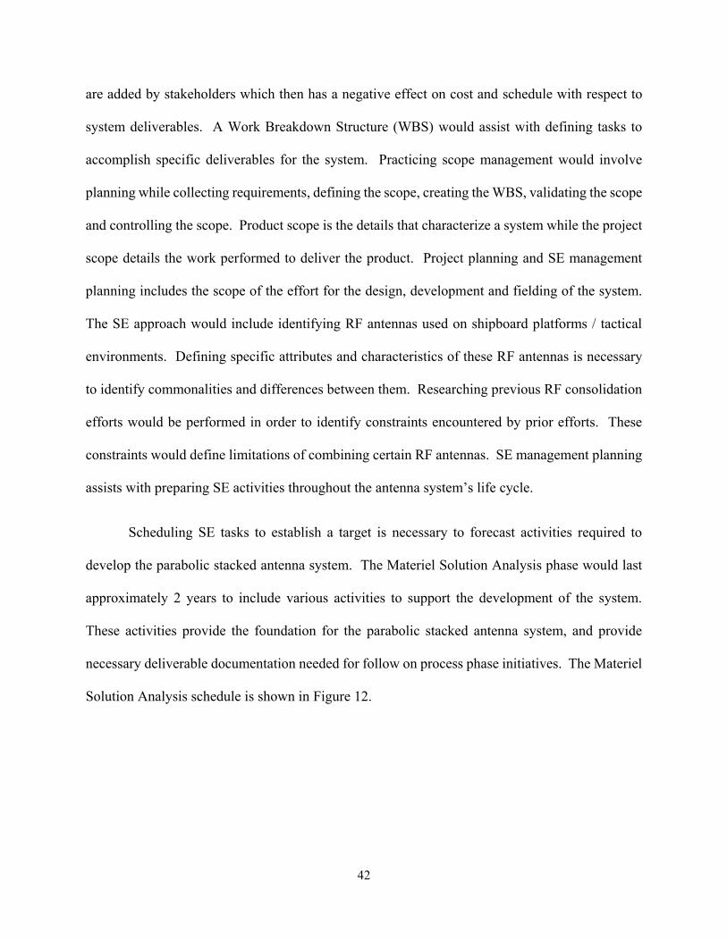
42

are added by stakeholders which then has a negative effect on cost and schedule with respect to

system deliverables. A Work Breakdown Structure (WBS) would assist with defining tasks to

accomplish specific deliverables for the system. Practicing scope management would involve

planning while collecting requirements, defining the scope, creating the WBS, validating the scope

and controlling the scope. Product scope is the details that characterize a system while the project

scope details the work performed to deliver the product. Project planning and SE management

planning includes the scope of the effort for the design, development and fielding of the system.

The SE approach would include identifying RF antennas used on shipboard platforms / tactical

environments. Defining specific attributes and characteristics of these RF antennas is necessary

to identify commonalities and differences between them. Researching previous RF consolidation

efforts would be performed in order to identify constraints encountered by prior efforts. These

constraints would define limitations of combining certain RF antennas. SE management planning

assists with preparing SE activities throughout the antenna system’s life cycle.

Scheduling SE tasks to establish a target is necessary to forecast activities required to

develop the parabolic stacked antenna system. The Materiel Solution Analysis phase would last

approximately 2 years to include various activities to support the development of the system.

These activities provide the foundation for the parabolic stacked antenna system, and provide

necessary deliverable documentation needed for follow on process phase initiatives. The Materiel

Solution Analysis schedule is shown in Figure 12.

43

Figure 12 Materiel Solution Analysis Schedule

The Technology Maturation and Risk Reduction phase is estimated to be a 2 year effort.

Reviewing system requirements to verify that the system is being designed within the

specifications would be performed during this phase. Developing a test and evaluation master plan

would begin in this phase as well. Producing guidance on how to perform testing allows how the

integrated product team would go about testing the system at a high level. Risk management

would continue through this phase to identify and mitigate risks. System engineering plan updates

would be completed along with developing safety documentation with respect to personnel and

the environment. A program protection plan entails how sensitive information is contained along

with any cyber security parameters. The PDR would occur to review the design and gain

concurrence from stakeholders. Another review would be the Technology Readiness Assessment

where the new technology would be analyzed to ensure the technology developed is mature and

feasible. Developing life cycle costs would depict estimated costs amongst the phases. The system

requirements document and the capability development document captures the system information

needed to establish the project to support the effort. Validating system support along with

maintenance objective requirements provide input to the integrated baseline review and support

44

plans. Additional inputs would be required for system threat assessments, the overall acquisition

strategy, affordability assessments and system safety documentation. The integrated baseline

review would occur to establish a collaborative concurrence amongst industry contractor partners

on system development. Completing these activities would reach Milestone B as shown in Figure

13.

Figure 13 Technology Maturation & Risk Reduction Schedule

The Engineering and Manufacturing Development phase is projected to span over 5 years.

This is a reduction of 3 years compared to the NMT project. Reducing schedule by 33% can be

forecasted by using Agile methodologies during the Engineering and Manufacturing Development

phase. A minimum range of a 9% to a median range of 33% schedule reduction was realized from

return on investment data gathered from over 300 scholarly articles [53]. The 33% schedule

reduction is used for the Engineering and Manufacturing Development phase for the parabolic

stacked antenna development to set a benchmark for project planning. Cost savings would be

realized with the amount of time required to deliver being reduced. During this phase, the system

45

is being designed and developed. Integration of various hardware, software and human systems

occur to produce the desired capabilities. Demonstrating the integration, interoperability,

supportability, safety and utility of the system through simulation and prototypes allow

stakeholders to observe system operation. Producibility is assessed to ensure the complexity to

manufacture the system is as low as possible. Determining the producibility complexity will

ensure that the system is affordable to produce. In addition to affordability, supportability of the

system would be assessed for operations and sustainment of the system. Demonstrating RAM of

the system provides insight to overall life cycle costs and sustainment needs. A Critical Design

Review (CDR) would be performed within the Engineering and Manufacturing Development

phase to gain concurrence to proceed to fabricate the design and create a prototype. The system

baseline would be established at the CDR and entail initial hardware specifications. The

Production Readiness Review (PRR) provides approval that the design is ready to be

manufactured. A Low Rate Initial Production (LRIP) can be agreed upon to begin producing an

initial set of systems. These activities would satisfy requirements needed to meet Milestone C as

shown in Figure 14.

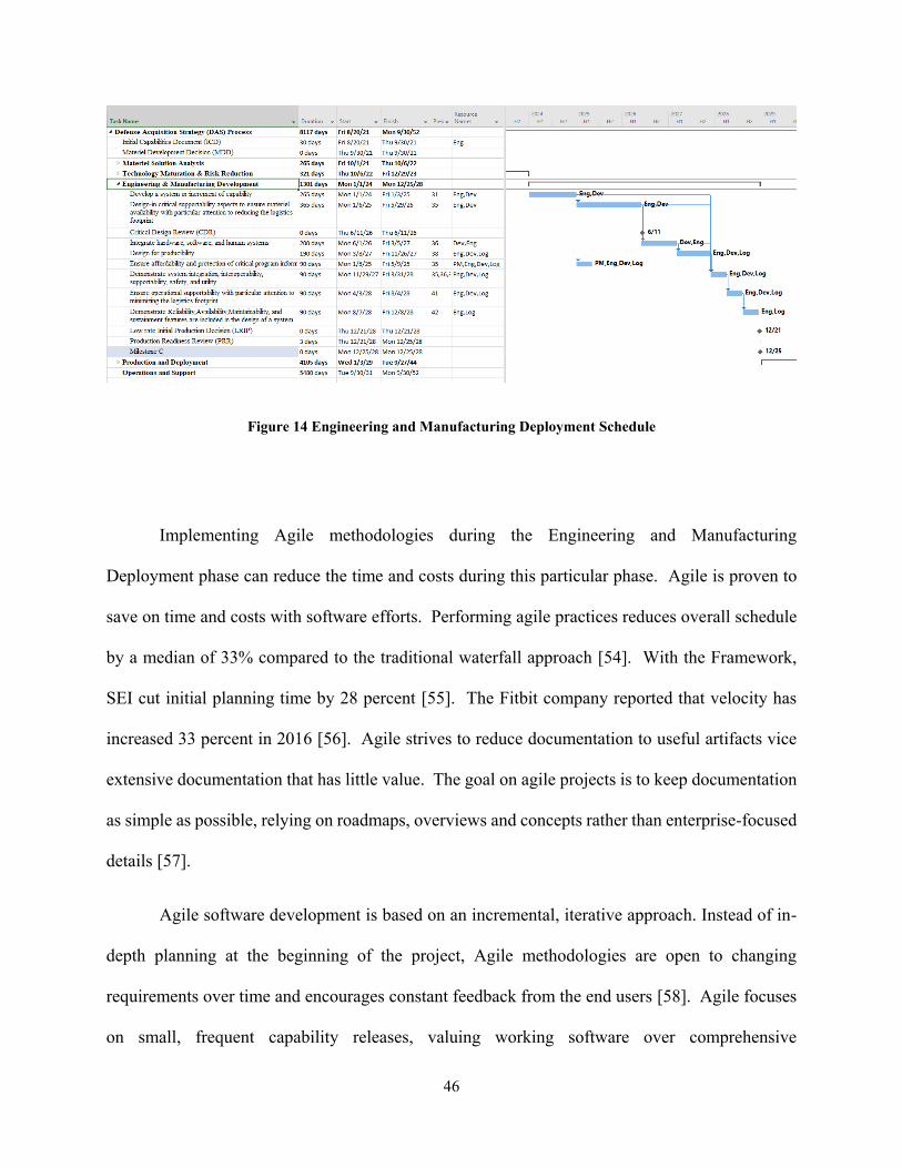
46

Figure 14 Engineering and Manufacturing Deployment Schedule

Implementing Agile methodologies during the Engineering and Manufacturing

Deployment phase can reduce the time and costs during this particular phase. Agile is proven to

save on time and costs with software efforts. Performing agile practices reduces overall schedule

by a median of 33% compared to the traditional waterfall approach [54]. With the Framework,

SEI cut initial planning time by 28 percent [55]. The Fitbit company reported that velocity has

increased 33 percent in 2016 [56]. Agile strives to reduce documentation to useful artifacts vice

extensive documentation that has little value. The goal on agile projects is to keep documentation

as simple as possible, relying on roadmaps, overviews and concepts rather than enterprise-focused

details [57].

Agile software development is based on an incremental, iterative approach. Instead of in-

depth planning at the beginning of the project, Agile methodologies are open to changing

requirements over time and encourages constant feedback from the end users [58]. Agile focuses

on small, frequent capability releases, valuing working software over comprehensive

47

documentation, responding rapidly to changes in operations, technology, and budgets, actively

involving users throughout development to ensure high operational value [59]. Releasing software

in increments allow the customer to evaluate, provide feedback and allow developers to make

adjustments. This strategy decreases the cost of overall changes made since the changes are done

early on rather than when an entire build is released.

The Agile Manifesto was created by seventeen developers and representatives from areas

such as Extreme Programming (XP), Scrum, Dynamic Systems Development Method (DSDM),

Adaptive Software Development, Crystal, Feature-Driven Development (FDD) and Pragmatic

Programming on February 11-13 of 2001. The goal was to find an alternative to documentation

driven, heavyweight software development processes [60]. The four values and twelve principles

that the agile manifesto included is listed in Table 5 below.

Table 5 Agile Manifesto [60]

Values

1 Individuals and interactions over processes and tools

2 Working software over comprehensive documentation

3 Customer collaboration over contract negotiation

4 Responding to change over following a plan

Principles

1 Our highest priority is to satisfy the customer through early and continuous delivery of valuable software.

2 Welcome changing requirements, even late in development. Agile processes harness change for the customer's competitive advantage.

3 Deliver working software frequently, from a couple of weeks to a couple of months, with a preference to the shorter timescale.

4 Business people and developers must work together daily throughout the project.

48

5 Build projects around motivated individuals. Give them the environment and support they need, and trust them to get the job done.

6 The most efficient and effective method of conveying information to and within a development team is face-to-face conversation.

7 Working software is the primary measure of progress.

8 Agile processes promote sustainable development. The sponsors, developers, and users should be able to maintain a constant pace indefinitely.

9 Continuous attention to technical excellence and good design enhances agility.

10 Simplicity--the art of maximizing the amount of work not done--is essential.

11 The best architectures, requirements, and designs emerge from self-organizing teams.

12 At regular intervals, the team reflects on how to become more effective, then tunes and adjusts its behavior accordingly.

The Agile Manifesto helped with creating a mindset for software development. Different

frameworks and methods can be used with this mindset to deliver software to the customer fast

and efficiently. Agile refers to various approaches such as Kanban, Scrum, XP, FDD, DSDM,

ScrumBan, and Agile Unified Process (AUP). A method is determined by what is best suited for

the team and the task involved. Kanban and agile are descendants of lean where they have shared

attributes. This shared heritage is very similar and focuses on delivering value, respect for people,

minimizing waste, being transparent, adapting to change and continuously improving [60]. Figure

15 depicts agile approaches for software development.

49

Figure 15 Agile Approaches [60]

Lean provides concepts such as eliminating waste, decreasing the amount of work queues

and delivering as much value as possible through value streams. Eliminating waste would include

assessing a particular process, and improving process areas to reduce the amount of work exerted

to accomplish a task which provides more value to the customer. Lean focuses on reducing

wasteful process steps and potentially reallocate resources to other quality work. Value is

determined by the customer with respect to the product or service being delivered and being

whether it is executed correctly. Identifying steps within a process while determining if that step

provides value and the customer is willing to pay for it is essential in reducing waste. Inefficiencies

in process areas can include information processing where automation could resolve excessive

time being spent to complete a task. Redundant process steps or steps that doesn’t add value to

the overall product or service should be reduced to save on time and costs. Personnel and facility

resources are also areas that can be assessed to reduce or eliminate waste. Bottlenecks that hinder

the flow of the process should be identified and assessed for potential process improvement

initiatives. The process should move in a continuous fashion and as fast as possible.

50

Kanban is a method for defining, managing, and improving services that deliver knowledge

work, such as professional services, creative endeavors, and the design of both physical and

software products [61]. Kanban improves communication and increases efficiencies within a

project through participation on a Kanban board. Kanban utilizes a visual board that has cards that

show tasks that can be worked on to deliver features to the customer. The visual board depicts

what tasks are in the backlog, are being working on, is in testing and is complete. These tasks that

are written on cards in the form of user stories move across the visual board to depict progress

from the beginning to the end. Team members are assigned on each task card to identify the

individual or individuals working the task. An example would include a Kanban board containing

columns for ready, develop and unit test, dev-done, system test and done as shown in Figure 16.

This methodology provides a visual depiction of status on particular tasking. Metrics can be

derived from Kanban such as cycle time of tasks, delivery rate and work in progress limitations.

Figure 16 Kanban Board Example [61]

51

Scrum is a framework within which people can address complex adaptive problems, while

productively and creatively delivering products of the highest possible value [62]. An agile scrum

team consists of main roles such as the product owner, scrum master and development team. The

product owner is the authoritative source that prioritizes / manages the backlog along with

communicating with the development team on the progress of their work. The scrum master

supports the product owner and ensures agile processes are being followed by the team. The

development team self organizes and works together to complete required tasks. A sprint is a

short, time-boxed period when a scrum team works to complete a set amount of work [63].

Breaking down large sized tasking into smaller manageable sprints allows for products to be

released faster with the intent of receiving feedback sooner. Receiving feedback sooner allows

changes to the product to be made sooner which makes change management more efficient.

Waiting to receive feedback once a product is fully designed and finished potentially creates a

costly change modification. Sprint planning begins with the team getting together to strategize

how they will be able complete a particular task and deliver a product. This planning would

include the amount of time the task is going to take, the objective, how the task is going to be

complete, who will be completing the task, and any dependencies required for the task to be

completed. A product backlog would contain a prioritized list of tasks that need to be completed.

This backlog of tasks is pulled by the team when the team members have capacity for it. These

tasks are called user stories which describes a user requirement. An epic is a group of stories

which represent a larger task. An initiative is a group of epics that focuses on a common objective.

A theme is the overarching focus area that represents a high-level effort. The daily scrum occurs

in the beginning of the day where the team, scrum master, and product owner discuss the tasking

they completed the previous day, the tasks they will be working on that day and if there are any

52

issues or blockages that are preventing them from making progress. A sprint review is conducted

to depict the work the team has produced for feedback and recognition. The sprint retrospective

allows the team to discuss what went well, what didn’t go so well and what areas needs

improvements. The product owner owns the product backlog while the sprint backlog is owned

by the team. These backlogs are prioritized and adjusted by the respective owners. The scrum

and sprint cycle is shown in Figure 17.

Figure 17 Scrum Sprint Cycle (after [64])

Development Operations (DevOps) is another methodology that promotes a collaborative

environment for developers, operators, and quality assurance personnel to work together. This

type of environment increases communication and builds trust between developers and operators.

Having this collaborative environment allows operator personnel to provide direct feedback to

developers early in the DevOps process. Defining and automating these processes decreases the

time for any software changes / releases. This collaborative environment assists with depicting

the lifecycle of the software from development to production. Quality assurance is an important

53

role that not only inspects the quality of the product but the quality of the processes to provide the

most efficient product as well. The DevOps methodology provides automated testing, continuous

integration, and continuous delivery. Deploying the software and receiving feedback improves

the software and the deployment of this software. Reducing rework and overhead will reduce time

which in turn saves on overall costs.

Scaled Agile Framework (SAFe) is for large organizations that operate at the portfolio,

program and team levels. With the metrics that SAFe provides combined with regularly reporting,

velocity has increased 33 percent [65]. With the Framework, the company SEI also cut initial

planning time by 28 percent, realized $30M in savings, shipped more than 350 production releases,

completed 22 PSIs over 125 sprints and delivered 250 features [55]. Organizations have realized

these benefits at a high level where lower levels within the organization would perform Agile

methods to deliver. The team level follows agile methods that deliver working software releases

over various sprints. The team meets every day during daily scrums as well as during spring

planning, sprint reviews, and sprint retrospective meetings. The program level consists of multiple

teams that deliver a larger software product. Program Increment (PI) Planning is a cadence-based,

face-to-face event that serves as the heartbeat of the Agile Release Train (ART), aligning all the

teams on the ART to a shared mission and Vision [66]. PI planning consists of teams that get

together to discuss the overall vision, business context, roadmap, features of the product and the

way forward. Establishing SAFe at a high level promotes collaboration amongst multiple projects

with multiple stakeholders which creates easier integration in efforts to deliver a product faster

and cheaper.

There are pros and cons for both waterfall and Agile methodologies. Using a waterfall

methodology such as the DAS process delineates schedule milestones. This can be used to better

54

estimate costs and depict a predictable schedule. Each phase of the waterfall requires specific

deliverables in order to proceed to the next phase which is typically determined by a review gate.

The waterfall methodology specifies certain document deliverables that are necessary to create

historical artifacts for future projects to use as a guide and to adopt lessons learned. These

documented deliverables provide updates to stakeholders on the progression of the project itself.

The waterfall method is well known throughout industry which would decrease the learning curve

for managing project efforts. The benefits of using Agile includes the project being flexible and

able to adapt due to shorter development cycles. These shorter development cycles allow for

stakeholder feedback to be received earlier on. This feedback would allow for changes to be made

immediately rather than later on which would potentially cause delay and increase cost of the

overall effort. Due to engineering a solution in increments via Agile sprints, unit tests can be

administered which verifies the overall solution. Quality is then increased due to the cycle of

engineering tests performed at each increment. In addition to a quality product, collaboration

amongst stakeholders is practiced throughout system development which increases productivity.

Agile unit tests allow engineering efforts to be verified and possibly adjusted with the early

phases of the system lifecycle. The waterfall approach has the potential to inadequately test a

product due to stringent schedule milestones. Inadequate testing can lead to a faulty system when

fielded. Tests that fail early on can be recovered easier using the Agile approach since a failed test

can be evaluated early on in development rather than producing and testing a larger deliverable

using the waterfall approach. Being able to change and catch issues as early as possible based on

stakeholder feedback can save costs and time using the Agile approach. The Agile approach is

acknowledged to provide rapid delivery of increments which would decrease delivery times. The

Agile approach increases stakeholder collaboration which increases overall productivity, but in

55

turn requires the commitment of time amongst stakeholders. The waterfall approach does have

benefits by having predictive schedule milestones with associated documented deliverables. Being

able to predict engineering efforts using the waterfall method enables easier budgeting for overall

efforts. Documented deliverables within a waterfall method demonstrates progress made to

stakeholders along with benefiting future endeavors of similar projects. The waterfall approach

requires gathering requirements early on which has the potential to create risk to cost and schedule

if a change is needed later on. The waterfall approach is well known and practiced throughout

industry while the Agile method may require additional training and buy in from stakeholders.

A combination of both waterfall and Agile methods is recommended to develop and deploy

a parabolic stacked antenna. The waterfall approach would be used to provide an overall predicted

schedule with an estimated budget. This estimated budget and time line is necessary for DoD

programs to allocate necessary resources for forecasted operational requirements such as

replacement of end of life systems and system consolidation efforts. Documentation requirements

shall be considered and tailored out to include vital information critical to project success and

future endeavors. Agile methods shall be used during early phases of the system life cycle to

include modeling, simulation, software development and integration activities. Stakeholder

commitment would have to be established early on by mutually acknowledging the benefits of

Agile and learning Agile methodologies.

The DoD instruction 5000.02 specifies management strategies and tailoring projects to

meet hardware and software product needs. A hybrid waterfall and Agile methodology can

provide much benefit. Hybrid approaches are introduced to account for parallel efforts regarding

hardware and software design and development. Software development would have to align with

the hardware being developed in order to have successful integration prior to Milestone C. Various

56

software builds would be planned based on the features required for the overall system. During

the technology maturation & risk reduction phase software would begin to be developed in

increments. The Engineering & Manufacturing Development phase would incorporate multiple

software builds to be incorporated and tested with the hardware platform. Later software releases

would occur during the production and deployment phase for any updates required when feedback

was received when the initial units were fielded. Figure 18 depicts a hybrid hardware / software

DAS process which does not depict updates during the operations and support phase of the life

cycle.

Figure 18 Hybrid Program [67]

Software and hardware updates would be performed during the operations and support

phase. These updates would be initiated by cyber security needs, RAM events or additional

capability features that are introduced over time. Disadvantages of the waterfall process includes

any new requirements or miscommunications of requirements will cost more by having to restart

57

the development process. Agile allows programmers to develop and provide prototypes to the

customer rapidly which gains immediate feedback which in turn reduces costly change requests.

The customer can provide feedback to the prototypes and the developers can make adjustments as

required.

Incorporating MBSE with Agile methods decreases the amount of time for design.

Releasing simulation results early on promotes obtaining sponsor feedback early on. By receiving

feedback from the customer early on, the design can continue or any changes that need to occur

can be made with minimal impact. If an iterative agile approach is not practiced, there is a chance

for increased risk that a major change may be required after the initial design is completed.

Simulations assist with learning about the system itself. By testing and validating system

characteristics early, models facilitate timely learning of properties and behaviors, enabling fast

feedback on requirements and design decisions [68]. During Program Increments (PI), simulations

can be produced to obtain results for further analysis. Figure 19 depicts MBSE incorporated within

an Agile fashion.

58

Figure 19 Models and Learning Cycles (after [68])

MBSE supports traceability, quality assurance, compliance verification, test results for

analysis / acceptance and depictions for interlinked dependencies. Producing MBSE models and

simulations for review while performing agile practices promote feedback to make any necessary

adjustments early on. Integrating the physical and virtual worlds validates virtual models and

helps engineers improve system analysis, better predict failures or downtime, and provide for more

accurate maintenance schedules [68]. Incorporating MBSE within an Agile framework reduces

the amount of time to develop and deliver designs.

Executing the DoD’s DAS process with respect to DoDI 5000.02 can be challenging when

incorporating Agile methodologies. Typical system engineering technical reviews can be replaced

with more frequent small reviews. Greater frequency allows key decision makers and other

stakeholders to become more familiar and comfortable with processes in the Agile environment,

which enables a more collaborative and productive review process [59]. The same amount of

59

engineering rigor is applied and allows for more frequent feedback in order to reduce the likelihood

of costly change requests. A change made early on can significantly be less costly and less time

consuming than a change made further down the process. Figure 20 depicts the correlation

between the DAS process and Agile methodologies.

Figure 20 DAS Process WRT Agile Methodologies [59]

Incorporating Agile methodologies within the DAS process can increase key stakeholder

collaboration, steer the direction the program is going and reduce time and cost with early change

requests. The waterfall approach provides a predictive schedule with a budget that can be

requested for in advance. Engineering rigor will still be in place by executing a hybrid approach

using waterfall and Agile methods. Cost and time savings can be realized by receiving stakeholder

feedback early on and making changes sooner than later. These cost and time savings can also be

60

realized by incremental testing using Agile practices which would capture issues early on as well

as increasing the quality of the system delivered.

The Production and Deployment phase would last for 8 years where the systems would be

manufactured and fielded during that time frame. This is a decrease of 3 years from the NMT

program’s production and deployment schedule. Reducing planned procurement actions required

for additional spares and antenna upgrades by procuring them in advance would assist with

decreasing the scheduled phase. Lessons learned and implementation of lean process improvement

initiatives allows for the reduction of the amount of years producing and deploying systems.

During this phase, various updates are implemented such as the product baseline, test and

evaluation plan, life cycle sustainment plan, safety plans, system engineering plan and cost data

for budgeting purposes. The Full Rate Production Decision review takes place to obtain

concurrence from stakeholders to proceed with manufacturing the systems at a large scale. Based

off of lessons learned and adjustments made after the initial set of systems were produced during

the LRIP, more refined systems are produced at a more efficient rate. The Production and

Deployment schedule is show in Figure 21.

61

Figure 21 Production and Deployment Schedule

The Operations and Support phase spans out for 22 years which will be the life of system,

and is equivalent to the life span of the NMT system. This phase will begin after the system is

fielded and operational. System operations along with maintenance and upgrades are performed

to meet mission requirements. Help desk support would be available within this phase to assist

with issues that surface during the life of the system. Metrics would be captured on issues

encountered to help alleviate recurring problems. Training would be provided during the

operations and support phase to enable system users to operate and maintain the system. Upgrades

and updates would be deployed or installed by SMEs based on complexity. Recurring system

checks are necessary to ensure the system is maintained and fully operational.

Average costs for the Technology Maturation & Risk Reduction phase is estimated at $5M

per year of RDT&E funding over 2 years based off of the NMT system cost data. The Engineering

& Manufacturing Development phase estimated at about $69.9M per year for RDT&E funding

over 8 years and $61.6M per year for procurement funding over a year. The Production and

Deployment phase had an estimated average value of $21.3M per year of RDT&E funding over

62

14 years and $72.6M per year of procurement funding over 18 years. The Production and

Deployment phase introduced Operating and Sustainment costs which began once the systems

were fielded. Using the average $87.6k per system fielded cost value the costs for performing

operation and sustainment tasks would reach $21.9M per year when 250 systems were fielded.

The estimated life cycle cost to develop and field the parabolic stacked antenna would be

$2227.2M which is $419.2M less than the NMT system. The NMT program had 2 years for the

Technology Maturation and Risk Reduction phase, 8 years for the Engineering & Manufacturing

Development phase, and 18 years for the Production and Deployment phase. The Operations and

Support phase overlaps a portion of the Production and Deployment phase and continues for 22

years which is approximately the life the NMT system. A recommended approach would include

utilizing key personnel that have been part of the NMT, CBSP and SDT programs to review lessons

learned and implement continuing process improvement recommendations to reduce the amount

of time to develop and field the parabolic stacked antenna. Implementing Agile methodologies

would reduce engineering costs and time lines by 33% which would potentially reduce the 8 year

amount that the NMT project operated within to approximately 5 years. The Production and

Deployment phase would be reduced by reducing the planned procurement actions required for

additional spares and antenna upgrades. Planning for shipboard availability and having the

personnel available to execute fielding actions is also essential for reducing costs and time.

Reduction of times would include reducing the Engineering & Manufacturing Development phase

by 3 years, and reducing the Production and Deployment phase by 3 years as well. The

Technology Maturation and Risk Reduction phase will be kept at 2 years and the Operations and

Support phase will be kept at 22 years to account for the life of the parabolic stacked antenna

system as well. Using average values of costs by the NMT program per year and per phase the

63

approximate costs were slated for each phase increment. Due to the reduction of time, and a phased

system deployment approach cost savings were realized. The Technology Maturation & Risk

Reduction phase would endure RDT&E costs of $10M, and the Engineering & Manufacturing

Development phase would endure RDT&E costs of $349.5M. The Production and Deployment

phase would endure RDT&E costs of $395.4 and $1089M of procurement costs. The RDT&E

costs during the production and deployment phase will support continuous improvement efforts

required with the system. The costs for the operations and support phase would be $383.3M which

is lower than the previous NMT program’s budget due to the amount of systems fielded at a slower

rate. The more systems fielded initially early on in the operations and support phase the more

costs are required to perform operations and support tasks. The approximate life cycle costs for

the parabolic stacked antenna system is shown in Table 6.

Table 6 Approximate Life Cycle Costs for the Parabolic Stacked Antenna System

Year RDT&E

Costs Procurement

Costs

Operations and

Sustainment Costs

Systems Ordered

QTY

Systems Fielded

Per Year Process Phase

2021 - - - - - Materiel Solution Analysis

Milestone A

2022 5 - - - - Technology Maturation & Risk

Reduction 2023 5 - - - -

Milestone B

2024 69.9 - - - -

Engineering & Manufacturing Development

2025 69.9 - - - -

CDR

2026 69.9 - - - -

2027 69.9 - - - - Operational Assessment / LRIP

2028 69.9 - - - -

Milestone C

2029 69.9 - - - - Production and

Deployment IOC

2030 69.9 72.6 - 25

64

Full Rate Production Decision Review

2031 21.3 72.6 2.2 25 25

Operations & Support

2032 21.3 72.6 4.4 25 50

2033 21.3 72.6 6.6 25 75

2034 21.3 72.6 8.8 25 100

2035 21.3 72.6 11.0 25 125

2036 21.3 72.6 13.1 25 150

2037 21.3 72.6 15.3 25 175

2038 21.3 72.6 17.5 25 200

2039 21.3 72.6 19.7 25 225

2040 21.3 72.6 21.9 - 250

2041 21.3 72.6 21.9 - -

2042 21.3 72.6 21.9 - -

2043 - 72.6 21.9 - -

2044 - 72.6 21.9 - -

2045 - - 21.9 - -

2046 - - 21.9 - -

2047 - - 21.9 - -

2048 - - 21.9 - -

2049 - - 21.9 - -

2050 - - 21.9 - -

2051 - - 21.9 - -

2052 - - 21.9 - -

Total 754.9 1089 383.3 250

Total Costs ($M) 2227.2

The service life for the NMT system is planned to be in operation for 22 years (FY 2012-

FY 2032) [69]. The DAS process was followed throughout time for to field NMT systems.

Planning for the next generation of multiband antennas that utilize the parabolic stacking

methodology to incorporate both NMT, CBSP and SDT operating frequency capabilities is

recommended to start in the near future. Historical and future planned amounts for the NMT

system included expending a total of $868.6M over 15 years. This included Research,

Development, Test and Evaluation activities throughout the DAS process. The DAS process

65

included the phases of Materiel Solution Analysis, Technology Maturation & Risk Reduction,

Engineering & Manufacturing Development and Production and Deployment. The Technology

Maturation & Risk Reduction phase begun after the Materiel Solution Analysis phase was

complete (Milestone A) in 2001. This led to a two year endeavor of Technology Maturation &

Risk Reduction tasking that valued at approximately $10M. Upon completion of the Technology

Maturation & Risk Reduction phase (Milestone B) in 2003, the Engineering & Manufacturing

Development phase begun to perform engineering activities until 2010. The Engineering &

Manufacturing Development phase was completed at Milestone C expending approximately

$559M. The completion of Milestone C consisted of the decision to begin Low Rate Initial

Production to begin fielding NMT systems. This decision led to the Production and Deployment

phase of the DAS process which expended approximately $217M of costs until 2019. The

Production and Deployment phase is still continuing until 2024 and has budgeted $81M throughout

the remaining years of this phase. Table 7 depicts annual RDT&E costs for the NMT system

throughout the DAS process.

Table 7 Annual RDT&E Costs for the NMT System (after [69])

Year -- -- -- -- -- Cost $M Process Phase

2000 Materiel Solution Analysis

Milestone A

2001 -- -- -- -- -- -- 3.4 Technology Maturation

& Risk Reduction 2002 -- -- -- -- -- -- 6.6

Milestone B

2003 -- -- -- -- -- -- 29.4

Engineering & Manufacturing Development

2004 -- -- -- -- -- -- 64.1

2005 -- -- -- -- -- -- 58.1

CDR

2006 -- -- -- -- -- -- 55.4

2007 -- -- -- -- -- -- 77.7

2008 -- -- -- -- -- -- 87.7

2009 -- -- -- -- -- -- 108.7

66

Operational Assessment / LRIP

2010 -- -- -- -- -- -- 78.8

Milestone C

2011 -- -- -- -- -- -- 18.1

Production and Deployment

IOC

2012 -- -- -- -- -- -- 17.5 Full Rate Production Decision Review

2013 -- -- -- -- -- -- 28.1

2014 -- -- -- -- -- -- 19.8

2015 -- -- -- -- -- -- 18.2

2016 -- -- -- -- -- -- 28.0

2017 -- -- -- -- -- -- 21.1

2018 -- -- -- -- -- -- 32.1

2019 -- -- -- -- -- -- 34.8

2020 -- -- -- -- -- -- 30.8

2021 -- -- -- -- -- -- 10.3

2022 -- -- -- -- -- -- 9.0

2023 -- -- -- -- -- -- 16.2

2024 -- -- -- -- -- -- 14.7

Total -- -- -- -- -- --868.6

Procurement costs include procuring the system from the manufacturer and installing the

system on the intended platform. The NMT system consisted of an antenna (s) and communication

group (s). Some variants included a group of antennas with one communication group rack, while

others consisted of a single antenna with a single communication group rack. The approximate

value of $1368M entails production and deployment costs associated with the NMT system. A

total of 250 systems were desired to be procured from 2010 where the LRIP was approved. The

quantities were spread out over 10 years to be funded incrementally. The production and

deployment phase only consisted of production and deployment efforts and did not include

RDT&E efforts which was separately budgeted in Table 8. The production and deployment phase

included tasks such as procuring the NMT system, procuring associated components (cables,

67

connectors, radomes, ancillaries, etc.), verifying system operation, installing the system, and

performing verification tests after the system was fielded. These efforts spanned across the years

of 2010 through 2028. The unit cost to produce and deploy a NMT system had an approximate

value of $5.5M per system when dividing the total value of $1368.4M over 250 systems.

Table 8 Annual Procurement Costs for the NMT System (after [69])

Year -- -- -- -- -- Cost $M System QTY Process Phase

Operational Assessment / LRIP

Engineering & Manufacturing Development

2010 -- -- -- -- -- -- 61.6 33

Milestone C

2011 -- -- -- -- -- -- 111.5 54

Production and Deployment

IOC

2012 -- -- -- -- -- -- 107.3 26 Full Rate Production Decision Review

2013 -- -- -- -- -- -- 156.2 34

2014 -- -- -- -- -- -- 183.6 41

2015 -- -- -- -- -- -- 233.2 17

2016 -- -- -- -- -- -- 118.1 12

2017 -- -- -- -- -- -- 38.4 2

2018 -- -- -- -- -- -- 68.1 8

2019 -- -- -- -- -- -- 95 10

2020 -- -- -- -- -- -- 71.4 13

2021 -- -- -- -- -- -- 11.1 -

2022 -- -- -- -- -- -- 25.5 -

2023 -- -- -- -- -- -- 14.4 -

2024 -- -- -- -- -- -- 20.7 -

2025 -- -- -- -- -- -- 17.4 -

2026 -- -- -- -- -- -- 14.7 -

2027 -- -- -- -- -- -- 12.7 -

2028 -- -- -- -- -- -- 7.5 -

Total -- -- -- -- -- --1368.4 250

68

Operation and sustainment costs involves maintenance for hardware and software

components of the NMT system. Depot maintenance with respect to sparing and repairs are

included in the operation and sustainment costs. These costs represent the NMT system to include

the antennas, communication groups and ancillaries associated with the system itself. Help desk

support is incorporated in to the operation and sustainment costs to provide onsite and offsite

troubleshooting support. Warehousing functions and storage costs for spares would include having

a stock of maintenance parts along with applicable spares for high failure rate items, and items that

are identified as single points of failure. Support for system life cycle testing would be included

to detect potential risk areas with hardware and software components. The annual costs for each

NMT system would be approximately $87.6k, while the annual cost to sustain the total amount of

250 systems would be approximately $21.9M. Assuming the CBSP sustainment cost mirrors the

NMT sustainment cost per system, a savings of $16.6M can be realized annually as shown in Table

9.

Table 9 Annual Operation and Sustainment Cost for the NMT System (after [69])

Cost Element

Cost per system

NMT $k

Cost for 250 NMT

systems $M

Cost for 190 CBSP

systems $M

Unit-Level Manpower 39.4 9.9 7.5

Maintenance 2.3 0.6 0.4

Sustaining Support 21.9 5.5 4.2

Indirect Support 24 6.0 4.6

Total 87.6 21.9 16.6

The total cost to develop and field the NMT system was estimated to be $2646.4M. This

total value included RDT&E, procurement, and operations and sustainment costs throughout a

span of approximately 32 years. The DAS process was followed to deliver the NMT capability to

the warfighter. The RDT&E costs ($868.6M) ranged from 2001 through 2024. The procurement

69

costs ($1368.4M) ranged from 2010 to 2028. Operations and sustainment costs ($409.4M) ranged

from 2011 to 2032. The total amount of systems ordered per year began in 2010 through 2020.

Giving a one year lag for the systems to be fielded from the prior ordering year provided an

estimated fielding range for years 2011 through 2021. The overall costs throughout the DAS

process over time for the NMT system is shown in Table 10.

Table 10 Approximate Life Cycle Costs for the NMT System (after [69])

Year RDT&E

Costs Procurement

Costs

Operations and

Sustainment Costs

Systems Ordered

QTY

Systems Fielded

Per Year Process Phase

- - - - - - Materiel Solution Analysis

Milestone A

2001 3.4 - - - - Technology Maturation & Risk

Reduction 2002 6.6 - - - -

Milestone B

2003 29.4 - - - -

Engineering & Manufacturing Development

2004 64.1 - - - -

2005 58.1 - - - -

CDR

2006 55.4 - - - -

2007 77.7 - - - -

2008 87.7 - - - -

2009 108.7 - - - - Operational Assessment / LRIP

2010 78.8 61.6 - 33 -

Milestone C

2011 18.1 111.5 2.9 54 33

Production and Deployment

Operations and

Support

IOC

2012 17.5 107.3 7.6 26 87 Full Rate Production Decision Review

2013 28.1 156.2 9.9 34 113

2014 19.8 183.6 12.9 41 147

2015 18.2 233.2 16.5 17 188

2016 28 118.1 18.0 12 205

2017 21.1 38.4 19.0 2 217

2018 32.1 68.1 19.2 8 219

2019 34.8 95 19.9 10 227

70

2020 30.8 71.4 20.8 13 237

2021 10.3 11.1 21.9 - 250

2022 9 25.5 21.9 - -

2023 16.2 14.4 21.9 - -

2024 14.7 20.7 21.9 - -

2025 - 17.4 21.9 - -

2026 - 14.7 21.9 - -

2027 - 12.7 21.9 - -

2028 - 7.5 21.9 - -

2029 - - 21.9 - -

2030 - - 21.9 - -

2031 - - 21.9 - -

2032 - - 21.9 - -

Total 868.6 1368.4 409.4 250

Total Costs ($M) 2646.4

Considering the similarities between the CBSP system and the NMT system, the total life

cycle costs for the CBSP system should be similar as well. In 2014, Harris was awarded an eight-

year $133 million contract from the U.S. Navy to provide 120 shipboard terminals on top of the

70 that were already provided that give access to high-bandwidth voice and data communications

[70]. 49 terminals initially were placed on Navy ships in 2009, and there were plans to issue an

additional 201 systems to the fleet after that [71]. The CBSP systems would consist of 190 fielded

systems on U.S. Navy platforms along with 250 NMT fielded systems. Operation and sustainment

costs in itself can be significantly reduced by fielding a parabolic stacked antenna capable of

functions that include SATCOM capabilities. Using the 22 year SATCOM system life cycle value

and assuming the sustainment costs for the CBSP system is the same as the NMT system, the

annual operation and sustainment costs for the NMT and CBSP systems with projected incremental

fielding is shown in Table 11.

71

Table 11 Annual Operation and Sustainment Costs for the NMT and CBSP Systems with Incremental

Fielding (after [69])

System Service Year

# of NMT Systems Fielded Cost ($M)

# of CBSP Systems Fielded

Cost ($M)

1 25 2.19 25 2.19

2 50 4.38 50 4.38

3 75 6.57 75 6.57

4 100 8.76 100 8.76

5 125 10.95 125 10.95

6 150 13.14 150 13.14

7 175 15.33 175 15.33

8 200 17.52 190 16.644

9 225 19.71 190 16.644

10 250 21.9 190 16.644

11 250 21.9 190 16.644

12 250 21.9 190 16.644

13 250 21.9 190 16.644

14 250 21.9 190 16.644

15 250 21.9 190 16.644

16 250 21.9 190 16.644

17 250 21.9 190 16.644

18 250 21.9 190 16.644

19 250 21.9 190 16.644

20 250 21.9 190 16.644

21 250 21.9 190 16.644

21 250 21.9 190 16.644 Total Cost over 22 Years 383.25 310.98

A cost savings of approximately $310.98M over 22 years can be realized in sustainment

costs alone if the NMT and CBSP systems were consolidated. This assumes that the systems

including the communication groups were consolidated and half the labor hours would be required

for maintaining one system vice two systems. Developing a parabolic stacked antenna system

capable of operating with both NMT and CBSP system capabilities would reduce costs. The

approximate life cycle costs for the parabolic stacked antenna system was $2,227.2M over 32

years. Considering life cycle costs for two systems would amount to approximately $4,454.4M

72

over 32 years. A life cycle cost savings of ~$2B over 32 years would be potentially realized by

developing one consolidated system vice two individual systems.

3.3 Requirements Engineering

IEEE 29148:2011 states that requirements engineering is concerned with discovering,

eliciting, developing, analyzing, determining verification methods, validating, communicating,

documenting and managing requirements [72]. The results of requirements engineering include a

set of high-level requirements decomposed into lower level requirements which can be verified,

validated, implemented and understood amongst various stakeholders. Discovering requirements

would include finding a need for improvement of an existing system / capability or a need for a

new system / capability. The need for topside antenna consolidation is an ongoing effort where

new capabilities are introduced to support the warfighter which require various types of antennas.

Elicitation of requirements consists of collaborating with stakeholders to establish a common

understanding, gain concurrence, and document requirements. Requirement elicitation would

have to take place where meetings may assist with acquiring high level requirements and the

overall vision. Documenting goals, objectives, and needs during these meetings would formulate

stakeholder requirements. Other requirement gathering techniques would include reviewing

current or historical documentation of a similar system. For antenna consolidation, reviewing

documentation on similar past engineering efforts included the development of Raytheon’s NMT

and Harris’s CBSP consolidated antennas. Any known existing engineering efforts would be

researched to potentially obtain information that can assist with developing the system.

Simulations, prototypes and modeling of the system promote requirement development as well.

Requirements would include the system along with the system’s life cycle. Developing

requirements would correlate to the overall need along with constraints, system objectives,

73

environment, operational scenarios, and interactions between users / systems with consideration

on the system’s life cycle. Analyzing elicited requirements would include reviewing the

requirements to ensure the requirements are complete, consistent, verifiable and unambiguous.

Identifying any requirement conflicts are also performed when analyzing. Trade-offs and

prioritization of requirements may need to occur in order to realistically achieve the required

criteria. Collaboration amongst stakeholders while capturing feedback and gaining concurrence

would ensure a common understanding of the requirements. Choosing a requirements

management tool assists with storing requirements within a central location along with traceability

of the requirements tend to be volatile, or additional requirements are added throughout the life

cycle. Rational DOORS Next Generation provides a smarter way to define, trace, analyze, and

manage requirements while complying with industry standards and regulations [73]. The Rational

DOORS Next Generation requirements management tool promotes understanding of

requirements, scope, and the associated costs. A centralized location to store and track

requirements is necessary for the life cycle of the system as shown in Figure 22.

74

Figure 22 Rational DOORS Next Generation Requirements Management Tool

Non-functional and functional requirements were listed to describe the system to be

designed to. Functional requirements define the functions of the system. Non-functional

requirements define the overall qualities or attributes of the resulting system [74]. Functional

requirements define the functions of the system. This requirements management tool has features

to track any adjustments and / or modifications made by placing a time stamp along with the user

that adjusted that requirement. Permissions to add, change, and delete requirements would be

made to manage control. The Rational DOORS Next Generation tool allows each requirement to

contain additional data. For instance, requirement 208597 would contain the RF antenna standards

profile shown in Table 12 within the database.

75

Table 12 RF Antenna Standards Profile [20]

Standards Categories Typical Standards

RF Transfer:

Frequency Range and Rate

Noise limits

RF Exposure

EMI Control

Goal: Operate within RF rules

and protocol

Broadcast standards Signal to noise ratio standards

FCC Regulations, IEEE C95.1 MIL-STD-461G, IEEE C63.12-

2015, IEEE C63.2-2009, IEEE C37.90.2-2004

Information Assurance:

RF COMSEC

Network Security

Physical Security

Software Security

Goal: Capable of passing an IA

audit

PKI, EKMS standards and protocol DISA Information Assurance

Support Environment Reqs. TEMPEST physical security

standards ISO/IEC 27034

RF Testing:

Standard Test Procedures for Antennas

Sites performing Emission testing Compliance of Transmitters Electrostatic Discharge Environmental RF Absorption

Goal: Perfrom and meet outlined

test procedures

IEEE 149-1977

IEEE C63.7-2015, IEEE C63.7-2005

IEEE C63.36-2015 IEEE C63.16-2016 IEEE 1613.1-2013 IEEE 1128-1998

Emissisons:

FM and TV Broadcast Receivers Land-Mobile Transmitters Low Voltage Electrical Equipment

Goal: Stay within acceptable RF

emissions boundaries

IEEE 187-2003

IEEE 377-1980 IEEE C63.4-2014

Safety:

RF Safety Program 3kHz to 300GHz Human Exposure to EMI

Goal: Adhere to RF safety

precautions

IEEE C95.7-2014

IEEE C95.7-2014, IEEE C95.1-2005, IEEE C95.3.1-2010

Disturbance:

Radio and IT Equipment

Radio Noise

Goal: Meet acceptable signal to

noise ratio requirements

IEEE C63.022-1996, IEEE C63.011-2000

IEEE C63.5-2006, IEEE C63.4-2003

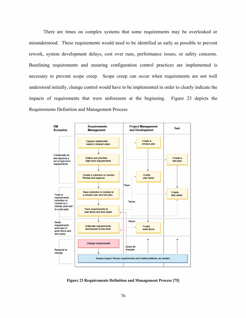
76

There are times on complex systems that some requirements may be overlooked or

misunderstood. These requirements would need to be identified as early as possible to prevent

rework, system development delays, cost over runs, performance issues, or safety concerns.

Baselining requirements and ensuring configuration control practices are implemented is

necessary to prevent scope creep. Scope creep can occur when requirements are not well

understood initially, change control would have to be implemented in order to clearly indicate the

impacts of requirements that were unforeseen at the beginning. Figure 23 depicts the

Requirements Definition and Management Process.

Figure 23 Requirements Definition and Management Process [75]

77

Requirements would be developed from particular needs. These needs would come from

strategic goals an organization or stakeholder envisions. Taking these needs and transforming

them into detailed requirements is necessary. A requirement is verifiable and is linked with

fulfilling a need. Measurable requirements are desired to determine if the objective has met a

specific threshold.

Identifying the RF antennas on a shipboard platform assisted with defining requirements.

Decomposed requirements to lower levels would specify antenna design criteria. Researching

prior antenna consolidation efforts defined limitations and constraints. Operational scenarios with

interfaces depicted interconnecting systems. System life cycle process concepts supported

identifying functional and non-functional requirements. Design requirements would include the

capability to create SATCOM and LoS links between systems. Cybersecurity requirements were

documented to ensure RF design compliancy was met. Cybersecurity requirements are important

to define early as well in the system’s lifecycle to prevent signal interception, jamming, and

intelligence data leaks. A newly designed fielded system that didn’t consider cybersecurity

requirements initially would cost more to mitigate than a system that is in the early stages of the

system’s life cycle.

Functional definition and analysis included translating requirements into functions. These

functions were grouped and allocated within specific groups associated with their frequency band.

Determining the nature of use for the parabolic stacked antenna system assisted with defining the

required functions. RF capabilities that operate concurrently with each other were specified along

with known interference problems of specified RF frequencies. Functional constraints identified

were defined for consideration during the design process. Testability needs were assessed for

future stand alone, integration, and operational verification.

78

Physical attributes were described and analyzed for form, fit, and function criteria.

Developing a system architecture model depicted the physical systems and platforms that

interconnected with one another. Identifying various assemblies and sub-assemblies described

mission parameters that the consolidated solution would be composed of. Each mission package

provides the operator specific RF communication capabilities. Design validation ensured the

proposed conceptual design aligned with system requirements. Simulating the RF solution proved

the benefit of having a consolidated antenna versus multiple antennas at different stages of the

system’s life cycle to perform common operations. Developing use case scenarios would further

prove required capabilities been met.

Cybersecurity risk management would involve identifying risks along with reducing the

likelihood and impact over a period of time. Designing the parabolic stacked antenna requires

consideration to the operational availability of the system. Anti-jamming measures would have to

take place to ensure RF communication services stay operational [19]. Incorporating a Low

Probability of Intercept / Low Probability of Detection (LPI / LPD) design is also essential to

maintain continuous communication links. Recurring audits would be required to ensure

compliancy of the system once it’s fielded. These audits would involve software, firmware,

Communication Security (COMSEC) equipment, and physical checks to ensure there are no

vulnerabilities or incidents present. Considerations for these checks would be documented during

the design of the parabolic stacked antenna. Security is essential when transmitting and receiving

sensitive data. As hackers and unauthorized users are attempting to cause malicious intent,

security measures are required to be put in place. A list of security features and functions

applicable to the parabolic stacked system are shown in Table 13.

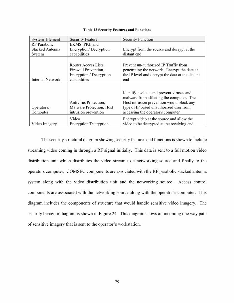
79

Table 13 Security Features and Functions

System Element Security Feature Security Function RF Parabolic Stacked Antenna System

EKMS, PKI, and Encryption/ Decryption capabilities

Encrypt from the source and decrypt at the distant end

Internal Network

Router Access Lists, Firewall Prevention, Encryption / Decryption capabilities

Prevent un-authorized IP Traffic from penetrating the network. Encrypt the data at the IP level and decrypt the data at the distant end

Operator's Computer

Antivirus Protection, Malware Protection, Host intrusion prevention

Identify, isolate, and prevent viruses and malware from affecting the computer. The Host intrusion prevention would block any type of IP based unauthorized user from accessing the operator's computer

Video Imagery Video Encryption/Decryption

Encrypt video at the source and allow the video to be decrypted at the receiving end

The security structural diagram showing security features and functions is shown to include

streaming video coming in through a RF signal initially. This data is sent to a full motion video

distribution unit which distributes the video stream to a networking source and finally to the

operators computer. COMSEC components are associated with the RF parabolic stacked antenna

system along with the video distribution unit and the networking source. Access control

components are associated with the networking source along with the operator’s computer. This

diagram includes the components of structure that would handle sensitive video imagery. The

security behavior diagram is shown in Figure 24. This diagram shows an incoming one way path

of sensitive imagery that is sent to the operator’s workstation.

80

Figure 24 Security Structural Diagram

The security behavior diagram in Figure 25 displays one way traffic of incoming video

data. The parabolic stacked antenna received encrypted video traffic and is decrypted by

COMSEC devices. The IP traffic within the encrypted RF signal is passed through the firewall

which permits or denies the incoming traffic. A network encrypt / decrypt device would remove

the encryption that encapsulated the data. The application security software would either accept

or deny the video then pass the video stream to the operator’s computer via UDP.

81

Figure 25 Security Behavior Model

The administrative portion with respect to security for the system includes risk reduction,

risk assignment, risk avoidance, and risk assessment which is handled by the communications

team. The communication team would be divided into sub-teams where the RF security, network

security, and workstation administrators assist with safeguarding sensitive information. The RF

security team would handle all the EKMS and PKI equipment necessary to ensure RF security is

met. Keying the equipment monthly would be required. Metrics such as the timeliness of keying

the COMSEC equipment monthly would be considered to identify any potential interruption of

82

services. This would reduce the risk of loss of service and assign the RF security team this duty.

The RF security team would avoid the risk of any malicious data by allowing the network security

and workstation administrative teams to account for any mishaps. The risk is accepted by the

organization to assume each sub-team performs their due diligence. The network team would be

responsible of updating access control lists and firewall entries. Metrics of the amount of malicious

data encountered would be assessed in order to tighten up the data security measures as necessary.

This would reduce the risk of any intrusions the network may have. The RF security portion is

avoided by the network security team by having the RF security team perform their duties.

Accepting this risk ensures SMEs are performing their functions within their team’s boundary.

The workstation administrative team would update security features for the operator’s computer

system. Metrics for the amount of malware encountered will be accessed and updated onto the

operator’s workstation. This would reduce the risk of malware being placed on the operator’s

workstation. The workstation administrative team would be assigned these duties and avoid the

risk of any RF or network related information assurance concerns by policing their functional area.

The organization would accept all risks with having these teams perform their duties in order to

have a safe information transferring system that is able to pass sensitive video to the operator’s

workstation securely. Security quality attributes have been documented within Table 14. The

assessment factors are shown to score the system’s security parameters is also listed. The potential

issues are described to identify any shortfalls that may be encountered.

83

Table 14 Security Quality Attributes

Quality Attribute Scoring System Potential Issues Predictability Updating security technical information

guidelines parameters monthly in order to predict potential intrusions, and malicious intent to do harm on the system. A 0 would indicate a poor job of predicting attacks where a 10 would indicate no attacks seen monthly.

Potential issues may include the security technical information guideline database is inoperable to obtain the latest information on how to protect the system.

Upgradability Upgradability would ensure all systems have the latest software patches needed to maintain compliance with all RF, Network, and computer appliances. A 0 would indicate outdated versions of software loaded on these appliances, where as a 10 would indicated all RF, Network, and computer appliances are up to date during an audit.

Potential issues could include licensing fees that may or may not be funded to upgrade to the latest version of any RF, Network or computer appliance. Another potential issue could be due to contract related limitations.

Effectiveness Effectiveness of the security would indicate if the system can safely pass data to the operator securely. A 0 would indicate frequent intrusions, attacks, viruses, and service discontinuations caused by malicious intent. A 10 would indicate no issues encountered related to the data security parameters.

Potential issues could include insider threat, where someone that has access to internal components may be able to breach the system.

Responsiveness Responsiveness would be scored by the timeliness of the RF, Network, or workstation administrative team reacts to a malicious encounter or breach. A 0 would indicate that there are numerous breaches with slow reaction times by the RF, Network or workstation administrative security teams. A 10 would indicate immediate responsiveness by the teams when a problem arises.

Potential issues could include lack of staff and / or funding to include the necessary SMEs to respond to issues within a timely manner.

Recoverability Recoverability would include the notion that if a security parameter is breached, how fast the system can be recovered back to a functioning state. A 0 would indicate an excessive outage for over a day. A 10 would indicate an outage for less than an hour.

Potential issues could include lack of trained staff, or equipment that would need to be completely replaced without having a spare on hand.

84

Designing RF systems to meet ongoing cybersecurity needs early will reduce or eliminate

the need for rework later in the system’s life cycle. Maintaining consistent continuity between RF

links while preventing malicious adversarial threats is critical for information assurance.

Performing ongoing risk management throughout the system’s life cycle is also beneficial to cost,

schedule, and performance parameters.

Identifying requirements early on will save on costs and prevent schedule delays at later

stages of the system life cycle. If requirements are not documented and agreed upon early, change

requests may be implemented in the future to satisfy the customer. This can affect a planned

budget, resource availability, and the planned schedule.

3.4 Concept Exploration and Benefits Analysis Phase

Needs assessment is an early phase SE activity area where real world needs are collaborated

with various stakeholders. Identifying these stakeholders that have an interest in the system would

take place to discuss needs which would be transformed into requirements. These stakeholders

includes, but is not limited to, users, operators, supporters, developers, producers, trainers,

maintainers, disposers, acquirer and supplier organizations, parties responsible for external

interfacing entities or enabling systems, regulatory bodies and members of society [72].

Collaborating with stakeholders requires different techniques to extract information relevant for

the system in need. Activities such as meetings, reviewing current / historical documents, market

analysis, modeling and simulating the system provides important information to capture needs for

requirement development.

Concept selection compares various alternatives with stakeholders to decide the best

Course of Action (COA) to take. Multiple COAs to be investigated are possible when potential

solutions are apparent amongst the alternatives. Concept selection is a recurring event throughout

85

the system’s life cycle that narrows down a set of potential solutions. Based off of the needs

captured from stakeholders, an assessment is performed to produce concepts that are feasible to

the design and development of the system. These concepts should be reviewed and analyzed for

trade off studies. When the needs are met with multiple concepts, criteria such as cost, schedule,

performance and risk would be researched to select the appropriate solution.

Producing a weighted matrix with these concepts where stakeholders would provide a score

to what they feel meets each need would narrow down a COA. Group decision making amongst

stakeholders assists not only with team cohesion but with selecting the best concept to move

forward with. Concurrence with selection criteria and applicable concepts lead to a concept

selected amongst stakeholders that acknowledges the risk and path to take. A concept screening

and weighted matrix assists a team with selecting the best concept to choose. This type of selection

process is repeated several times throughout the system's life cycle when alternatives are present

to pose as a viable solution. This concept screening and weighted matrix provides an artifact to

refer to when future questions arise on how a concept, course of action or solution was selected.

A concept screening matrix would assist with various concepts for selecting the most feasible

solution. The concepts would be listed in the upper columns while the selection criteria would be

listed to the left most column. The selection criteria is tied to high level requirements and

prioritized. Comparing these concepts would eliminate concepts that would not meet the selection

criteria.

The remaining concepts would be evaluated with weights. These weights depict the

importance of each selection criterion. Ratings are assigned to each concept corresponding with

the selection criterion. The team would select the appropriate rating based on their own and SME

judgement. The ratings and weights are multiplied to produce a value to compare. These values

86

would be compared amongst the concepts to select the highest value. If there are concepts that

produce the same overall value when comparing, additional selection criteria may be added to

select the most feasible concept. A closer look at these concepts may reveal additional facts.

Selection criteria associated certain customer needs may not include factors such as part

availability, ease of production, ease of design, specific details on how to produce the concept and

so on. Risks can be introduced to further down select or choose a concept. New technology can

pose risk when data on the life cycle of a new technology may be minimum.

The Pugh Matrix is a type of matrix diagram that allows for the comparison of a number

of design candidates leading ultimately to which best meets a set of criteria [76]. Table 15 depicts

design concepts to meet the requirements for a consolidated antenna. A fully adjustable dish with

a fully adjustable feed antenna system was set as the baseline within the Pugh Matrix. This design

would satisfy the requirements; however other solutions are applicable to meet the criteria. A fully

adjustable dish with multiple feeds would satisfy requirements as well as multiple non-adjustable

dishes with multiple feeds. These designs were compared within the Pugh matrix to determine

which concept is better than the other. This type of matrix is recommended to be performed with

appropriate stakeholders to obtain concurrence on the best course of action. The fully adjustable

dish and fully adjustable feed antenna system was set as the baseline where an “S” was placed in

each criteria. A “+” or “++” was used to show if the design concept was better / much better than

the baseline. A “-” or “- -” was used to show if the design concept was worse / much worse than

the baseline. Weights were assigned to express the importance of specific selection criteria. The

total value added the amount of “+” or “-” shown with each design concept with respect to

multiplying the applicable weights.

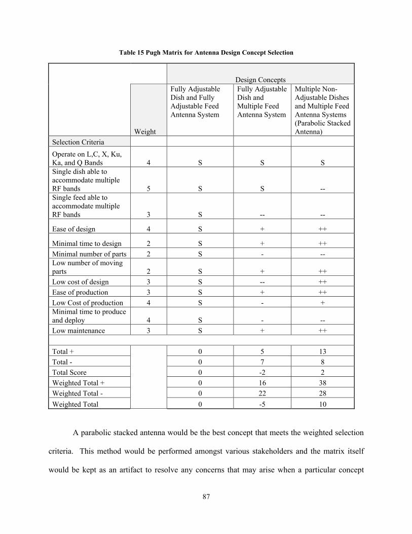
87

Table 15 Pugh Matrix for Antenna Design Concept Selection

Design Concepts

Weight

Fully Adjustable Dish and Fully Adjustable Feed Antenna System

Fully Adjustable Dish and Multiple Feed Antenna System

Multiple Non-Adjustable Dishes and Multiple Feed Antenna Systems (Parabolic Stacked Antenna)

Selection Criteria

Operate on L,C, X, Ku, Ka, and Q Bands 4 S S S Single dish able to accommodate multiple RF bands 5 S S -- Single feed able to accommodate multiple RF bands 3 S -- --

Ease of design 4 S + ++

Minimal time to design 2 S + ++

Minimal number of parts 2 S - -- Low number of moving parts 2 S + ++

Low cost of design 3 S -- ++

Ease of production 3 S + ++

Low Cost of production 4 S - + Minimal time to produce and deploy 4 S - --

Low maintenance 3 S + ++

Total +

0 5 13

Total - 0 7 8

Total Score 0 -2 2

Weighted Total + 0 16 38

Weighted Total - 0 22 28

Weighted Total 0 -5 10

A parabolic stacked antenna would be the best concept that meets the weighted selection

criteria. This method would be performed amongst various stakeholders and the matrix itself

would be kept as an artifact to resolve any concerns that may arise when a particular concept

88

selected is questioned. Comparing the concepts with associated weights allows a group of

stakeholders to collaboratively select a particular concept.

The parabolic stacked antenna system would provide various beneficial service features to

the warfighter. Services to include internet, voice, data, and real time imagery would allow the

user to accomplish mission objectives. Using these capabilities the warfighter would be able to

upload and download data along with other functions such as search, view, store as well as send

and receive various types of information to include encrypted voice or data. Mission services

include the communication plan which identifies the communication requirements of the user.

These communication requirements define what satellite the user is needing to connect to along

with other relevant configurations. The communication plan is submitted to the appropriate

approval authority to provide access to a particular satellite. Data links between SATCOM and

LoS operations are established to achieve operational mission requirements. LoS operations using

the CDL protocol would allow information sharing for surveillance and reconnaissance operations.

Enterprise services would provide overarching mission services across multiple entities.

Enterprise services provide cross domain, interoperable solutions consisting of multiple

capabilities. The parabolic stacked antenna capable of providing SATCOM and LoS operations

assist with providing enterprise capabilities that span across multi-platform mission operations.

Mission services provide various data transfer operations such as COMSEC, RF,

Networking, and video streaming. RF services would include wireless links to satellites or other

antennas capable of LoS. This entails transmitting and receiving information over relevant RF

bands. In addition to RF services, COMSEC services is critical to encrypt and decrypt data traffic.

Keying Material (KEYMAT) is typically used on data to protect sensitive information from

adversaries. The source and destination would have corresponding KEYMAT to unlock the data

89

that is transferred. This KEYMAT is changed periodically which is based on COMSEC policy to

secure data. Networking services is also involved with communication systems by routing data

using IP addresses and other routing protocols. Video streaming services would utilize networking

and COMSEC services in order to deliver live imagery to the user securely. Infrastructure

resources such as COMSEC, networking, video distribution, and RF equipment is used to provide

services to the user.

A layered architecture was developed to show interacting interfaces among layers.

Dependencies of lower echelon services are shown in Figure 26. The services included user,

mission, system (COMSEC, RF, Network, Video Stream), and enterprise. The infrastructure

resources were also included in this model.

90

Figure 26 Parabolic Stacked Antenna Layered Service Architecture

91

The service taxonomy was composed to list services for three domains. The three domains

included Ground_Comms, Shipboard_Comms, Mobile_Comms. These domains have services in

which communication among them would have to occur in order to accomplish mission

requirements. Values and operations were added to the parabolic stacked antenna service

taxonomy to depict the characteristics of the system service. The parabolic stacked antenna service

taxonomy is shown in Table 16.

Table 16 Parabolic Stacked Antenna Service Taxonomy

System Service Use Cases Domains Domain Services Values Operations

Communications::

Establish a

connection with a

satellite to send and

receive data

Obtain

SATCOM

connection

Ground

Comms

Transmit Data

Receive Data

Acquire Satellite

Track Satellite

LoS

SATCOM

Wireless

Receive

Transmit

Shipboard

Comms

Mobile

Comms

Internet::Establish a

connection with the

internet

Utilize

Internet

Traffic

Ground

Comms

Access WWW

Use Email

Transfer Files

View Videos

IP_Address

Port

Protocol

Allow

Block

Configure

Connect

Route

Shipboard

Comms

Mobile

Comms

Full Motion Video

(FMV) Distribution:

Video distributed

during a mission

Streaming

FMV over a

line of sight

(LoS)

connection

Ground

Comms

Establish LoS

connection

Send video

Receive video

Audio

Metadata

Video

Broadcast

Multicast

Unicast

The contextual perspective diagram was developed to depict the relationships of full

motion video distribution. Operators in various domains would utilize interconnecting services in

order to achieve the capability of sending and receiving video. This video would be analyzed and

used to evaluate potential strategies to accomplish mission objectives. This context diagram is

shown in Figure 27.

92

Figure 27 FMV Distribution Service Context Diagram

MBSE played a key role in early phase system engineering. Utilizing MBSE SysML

contributed to developing parabolic stacked antenna service architectures, context diagrams,

sequence diagrams and system architectures. Context diagrams depicted interconnecting services

93

with communication platforms in relation with operators to illustrate mission objectives. Sequence

diagrams provided various activities for the parabolic stacked antenna which were mapped to

particular entities performing these functions. Service architectures provided a decomposed view

of operations that is required by the user for both the mission and the enterprise level. These

models assisted with determining parabolic stacked antenna design requirements, assessing

interconnections among RF systems and parabolic stacked antenna project planning

considerations. In addition, developing these models assisted with identifying similar capabilities

between SATCOM systems currently fielded. The MBSE SysML system architecture shown in

Figure 4 in Section 3.1 identified that the CBSP and NMT communication groups had similar

operational services such as NIPRNet, SIPRNet, secure communications and imagery distribution.

This diagram also identified that the CBSP and NMT communication groups both have the

capability of operating at K, Ka and X band frequencies. Identifying these redundant capabilities

amongst different antenna systems further stresses the need to consolidate antennas to reduce

antenna overcrowding on the topside of U.S. Navy shipboard platforms. MBSE assisted with

identifying antenna system operating frequency bands of the CBSP, NMT and the directional SDT

antenna system variants which were used to simulate with parabolic stacked antenna

configurations in Section 4.

94

4. Antenna Consolidation via Parabolic Antenna Stacking Synthesis

Parabolic antenna stacking combines multiple RF antennas on a single pedestal.

Performing this method eliminates the need for multiple antennas on multiple pedestals. In a space

constrained environment such as military shipboard platforms, the need to consolidate RF antennas

is desired. A combined L-Band (1-2 GHz) and Ka-Band (20-30 GHz) antenna was patented in

January 2013 that consisted of a dual-reflector antenna comprising a backfire helix using the sub-

reflector as its reflector [77]. This combined antenna allowed multiple frequency capabilities to

be achieved. This concept proved that stacking parabolic antennas in front of one another would

successfully achieve multiband frequency needs for a space constrained environment. Six types

of antenna configurations are investigated and compared against using the parabolic stacked

antenna method. These antenna configurations included the Cassegrain with Gregorian parabolic

stacked antenna, Gregorian with splash plate parabolic stacked antenna, the dual Gregorian

parabolic stacked antenna, the dual splash plate parabolic stacked antenna, triple Cassegrain

parabolic stacked antenna and the dual Cassegrain with splash plate antenna. These parabolic

stacked antenna configurations were modeled through Antenna Magus software to obtain the

physical parameters and simulated through CST Microwave Studio software to obtain VSWR,

gain, radiation pattern, side lobe and angular width (3 dB) results.

The Cassegrain antenna has a primary and secondary reflector and is capable of reaching

high RF signal gains. The feed horn extrudes out of the center of the primary parabolic dish

transmitting and receiving RF signals. Advantages of the Cassegrain antenna include the feed

radiator is more easily supported, the antenna is geometrically compact, and it provides minimum

losses as the receiver can be mounted directly near the horn [78]. The physical dimensions of the

Cassegrain antenna is shown in Figure 28.

95

Figure 28 Physical Dimensions of a Cassegrain Antenna [79]

The feed of the antenna is placed in the center of the main parabolic dish and is connected

to the rear of the dish in which the RF signal is provided. The RF signal is reflected off of the

secondary reflector dish and sent back to the primary parabolic dish where the RF beam is formed.

The RF beam is formed with the RF signal sent out of the feed horn at an angle against the

secondary parabolic dish reflecting the signal to the primary parabolic dish forming a beam as

shown with parallel lines in Figure 29.

96

Figure 29 Cassegrain Antenna Ray Collimation after [80]

The blockage area shown in front of the sub-reflector on the Cassegrain antenna identifies

space that can be allocated for another parabolic antenna to stack. Other antennas can use the same

methodology as long as they incorporate some sort of sub-reflector. The sub-reflector reflects the

signals coming from the feed where a virtual feed shown as the parabola focal point in Figure 29

can provide the same signal pattern if the sub-reflector was not physically there denoted by the

dotted lines coming from the parabola focal point. The parabolic focal point is calculated by the

diameter of the dish D and the depth of the dish d.

𝒇𝒐 = 𝑫𝟐𝟏𝟔𝒅 (1)

The Gregorian antenna is a parabolic antenna that was researched for the parabolic antenna

stacking methodology as well. This dual reflector antenna is similar to the Cassegrain antenna

where the main difference is the shape of the sub-reflector. The sub-reflector for the Gregorian

antenna concaves inward toward the primary dish while the sub-reflector for the Cassegrain

antenna has a convex sub-reflector that curves outward as shown in Figure 30. The reflection

97

pattern from the sub-reflector for each of the Cassegrain and Gregorian antenna would produce

slightly different reflection patterns due to the shape of their sub-reflectors.

Figure 30 Physical Dimensions of a Gregorian Antenna [81]

The feed of the Gregorian parabolic antenna is placed in front of the dish where part of the

feed goes through the primary dish to the rear of antenna. The concave sub-reflector reflects the

signal back to the primary dish to be sent to the distant end. The Gregorian antenna transforms

the low to medium gain radiation of the feed horn to a high-gain pencil beam [81]. Similar to the

Cassegrain antenna, the sub-reflector of the Gregorian antenna creates a blockage area where

another antenna can be stacked in front to utilize the blocked area. Figure 31 depicts the Gregorian

antenna ray collimation.

98

Figure 31 Gregorian Antenna Ray Collimation [82]

The splash plate antenna is another parabolic antenna that can be used for parabolic antenna

stacking. The splash plate antenna (also known as the hat fed parabolic antenna) was investigated

to provide multi-band frequency capabilities. The splash plate antenna is fed from behind the

reflector dish reducing the amount of blockage that other parabolic reflector antennas have. The

splash plate is easy to install, has low aperture blocking and is cheap to produce [83]. In Very

Small Aperture Terminal (VSAT) communications, the use of splash plate antennas has been

increasing due to its’ compactness [84]. With this compactness feature, multiple splash plate

antennas would be used on a single antenna pedestal to provide multiple frequency capabilities.

The splash plate parabolic antenna is comprised of a primary dish reflector, waveguide, dielectric

lens and sub-reflector. The dielectric lens supports the sub-reflector which reduces interference

which other antenna aperture structures may introduce. Dielectrics such as Teflon

polytetrafluoroethylene (PTFE) would be used due to is temperature stability of -260°C to +260°C,

loss tangent ( δ) of .0004, and dielectric constant (εr ) of 2.1 [85]. Dielectric constant represents a

material’s ability to store electrostatic energy in an applied electric field [86]. Dielectric materials

have characteristics of having the ability of becoming polarized and are poor electric conductors.

The higher the value of the dielectric constant, the lower the gain and bandwidth [87]. In addition

99

to the dielectric constant of material, the materials’ loss tangent is important as well. As the loss

tangent of the material increases, the antenna gain decreases [88]. The strength of the PTFE varies

with temperature. The colder the temperature the stronger the material is. Teflon by DuPont resin

may be chosen in preference to other materials because of its better chemical resistance, heat

resistance, friction coefficient, dielectric strength, toughness, weather resistance, or combination

of such properties [89]. Figure 32 lists the PTFE dielectric material strength associated with its

corresponding temperature value.

Figure 32 PTFE Dielectric Strength at Various Temperatures [89]

The splash plate secondary reflector is held by the dielectric material to reflect the RF

signal back to the main dish which is reflected outward. The splash plate antenna is similar to the

Gregorian and Cassegrain antenna where signals are reflected off of the secondary dish, and the

secondary dish creating a blockage zone on the non-reflecting side. The splash plate antenna ray

collimation shown in Figure 33 depicts the RF signal reflection off of the parabolic dish.

100

Figure 33 Splash Plate Antenna Ray Collimation [10]

Engineering software for antenna design assists with modeling and simulation. Antenna

Magus is a software tool to help accelerate the antenna design and modeling process [90]. The

software provides alternatives as well as adjusting physical aspects of an antenna based off of

specifications entered in. A splash plate antenna was used to demonstrate Antenna Magus’s and

CST Microwave Studio’s capability to produce an antenna to support various frequencies.

Frequencies used by the CBSP, NMT and directional SDT antennas were entered into the software

to obtain physical and logical outputs for a splash plate antenna. The physical parameters for the

splash plate antenna as shown in Figure 34.

101

Figure 34 Physical Dimensions of a Splash Plate Antenna [91]

The splash plate feed uses backfire radiation to illuminate the dish, and the feeder

waveguide doubles as a feed/support structure [92]. This is a compact reflector topology with the

feed positioned close to the main reflector requiring no additional support struts. Another

advantage is that the feed antenna can be fed from behind the main reflector, reducing unwanted

aperture blockage. Antenna Magus and CST Microwave Studio was used to obtain VSWR values

and radiation pattern information for the frequencies that the NMT, CBSP and directional SDT

antennas support. As the frequencies increase, the size of the antenna decreases to conform to

NMT, CBSP and directional SDT frequency capabilities.

Various metrics were obtained to assess antenna characteristics. The VSWR values, gain,

radiation pattern, side lobe values and angular width (3 dB) values for each parabolic stacked

antenna configuration were captured after simulating each arrangement in CST Microwave Studio.

102

VSWR is an indication of the amount of mismatch between an antenna and the feed line connecting

to it, and a VSWR value under 2 is considered suitable for most antenna applications [93]. VSWR

(2) is solved by incorporating the reflection coefficient Γ, where the reflection coefficient (3)

involves the relationship between the reflected power Pref and forward power Pfwd. In the context

of antennas and feeders, the reflection coefficient is defined as the figure that quantifies how much

of an electromagnetic wave is reflected by an impedance discontinuity in the transmission medium

[94].

𝑽𝑺𝑾𝑹 = 𝟏+|𝚪 |𝟏−|𝚪 | (2)

𝚪 = √ 𝐏𝐫𝐞𝐟𝐏𝐟𝐰𝐝 (3)

The antenna gain was captured during the simulations to assess the strength of the RF

signal. The antenna gain G is over an isotropic source and is denoted as dBi. Antenna gain is the

relative measure of an antenna’s ability to direct or concentrate radio frequency (RF) energy in a

specific direction or pattern [95]. The antenna gain (4) relates to antenna efficiency 𝒌 measured

as a percentage, diameter of the parabolic reflector D measured in meters, and wavelength 𝛌 which

is measured in meters as well. Antenna efficiency (5) correlates to the wavelength, diameter of

the parabolic dish, and gain.

𝐆 = 𝟏𝟎𝐥𝐨𝐠𝟏𝟎 𝒌 (𝛑𝐃𝛌 )𝟐 (4)

𝒌 = ( 𝛌𝛑𝐃)𝟐 (𝟏𝟎) 𝐆𝟏𝟎 (5)

103

CST Microwave studio was able to produce antenna efficiency results in dB. To convert

the dB value to a percentage formula (6) is used to obtain the value. Consequently, to convert the

antenna efficiency percentage back to a dB value equation (7) is used.

𝒌𝒑𝒆𝒓 = (𝟏𝟎)𝒌𝒅𝑩𝟏𝟎 (6)

𝒌𝒅𝑩 = 𝟏𝟎𝐥𝐨𝐠𝟏𝟎 (𝒌𝒑𝒆𝒓) (7)

Side lobe data was recorded with each parabolic stacked antenna configuration. Side lobes

are usually radiation in undesired directions which can never be completely eliminated [96].

Another value recorded was the angular width (3 dB) of the output signal. The 3 dB, or half power,

beam width of the antenna is defined as the angular width of the radiation pattern, including beam

peak maximum, between points 3 dB down from maximum beam level (beam peak) [97]. As the

gain of the antenna increases the beam width decreases. The beam width at half power 𝐵𝑊𝐻𝑃

also known as angular width (3 dB) relates to wavelength 𝛌 and parabolic antenna diameter D as

shown in equation (8).

𝑩𝑾𝑯𝑷 = 𝟕𝟎𝛌𝐃 (8)

Signal transmission characteristics were captured using CST Microwave Studio while

Antenna Magus software was able to capture the physical parameters of the parabolic antennas.

Consolidating antennas via parabolic antenna stacking allows multi-frequency capabilities to be

achieved on a single antenna pedestal. The Cassegrain, Gregorian and splash plate antennas are

104

analyzed to propose parabolic stacked antenna configurations. The Cassegrain, Gregorian and

splash plate antenna were researched to provide a single pedestal solution for consolidating the

CBSP, NMT and directional SDT variant antennas. The Cassegrain, Gregorian and splash plate

antenna have unique characteristics to operate at various frequencies. Details on their physical

parameters and signal transmission characteristics are described in this section.

Parabolic antenna stacking involves using the blockage area that a parabolic antenna with

sub-reflector produces. Additional antennas is used within these blockage areas to support

multiple antennas on a single pedestal to achieve multi-frequency capabilities. The diameter of

the large parabolic antenna sub-reflector 𝑫𝒏𝒔𝒖𝒃would be greater than or equal to the diameter of

the smaller main parabolic antenna dish 𝑫𝒏𝒎𝒂𝒊𝒏. Multiple antennas would be stacked in front of

one another as far as the blockage area permits on each parabolic reflector antenna as shown in

equation (9).

𝑫𝟏𝒔𝒖𝒃 ≥ 𝑫𝟐𝒎𝒂𝒊𝒏 𝑫𝟐𝒔𝒖𝒃 ≥ 𝑫𝟑𝒎𝒂𝒊𝒏 (9) 𝑫𝟑𝒔𝒖𝒃 ≥ 𝑫𝒏𝒎𝒂𝒊𝒏 ….

4.1 Cassegrain with Gregorian Parabolic Stacked Antenna

The Cassegrain with Gregorian parabolic stacked antenna provides SATCOM and LoS

frequency band operations. These frequencies are operated within currently fielded NMT Q / Ka,

NMT X / Ka and SDT antennas. This configuration also achieves CBSP antenna capable

frequencies with the exception the L band frequency range (.95 GHz to 2.05 GHz) and the C band

105

frequency range (3.7 GHz to 4.2 GHz). A large Cassegrain antenna is used to operate at lower

frequency bands while a smaller Gregorian antenna is stacked in front of the Cassegrain antenna’s

sub-reflector to operate within higher frequency bands. The parabolic stacked antenna geometry

is shown in Figure 35.

Figure 35 Cassegrain and Gregorian Parabolic Stacked Antenna Geometric Properties

The Cassegrain antenna’s total length 𝐿𝑡𝐶 incorporates the diameter of the sub-reflector 𝐷𝑆𝐶,

distance between the main dish and foci 𝐹𝐶, half of the major axis of the ellipse 𝑎𝐶, and half of the

distance between the foci 𝑓𝐶 [98].

𝑳𝒕𝑪 = 𝑭𝑪 + 𝒂𝑪√𝟏 + 𝑫𝑺𝑪𝟐𝟒(𝒇𝑪𝟐−𝒂𝑪𝟐)− 𝒇𝑪 (10)

106

Half of the distance between the foci 𝑓𝐶 for the Cassegrain antenna is determined by the

diameter of the main parabolic dish 𝐷𝑚𝐶 , position of the secondary focus 𝐿𝑠𝐶, angle to the edge

ray of the sub-reflector 𝜃𝑒𝐶and the distance between the main dish and foci 𝐹𝐶 [98].

𝒇𝑪 = 𝑳𝒔𝑪[−𝑫𝒎𝑪−𝟒𝑭𝑪 𝐭𝐚𝐧𝜽𝒆𝑪𝟐 ]𝟐𝝈𝑫𝒎𝑪 (11)

The total length of the Cassegrain antenna 𝐿𝑡𝐶 with respect to the main parabolic dish and

sub-reflector is found by incorporating equation (11) into equation (10).

𝑳𝒕𝑪 = 𝑭𝑪 + 𝒂𝑪√𝟏 + 𝑫𝑺𝑪𝟐𝟒(𝒇𝑪𝟐−𝒂𝑪𝟐)− 𝑳𝒔𝑪[−𝑫𝒎𝑪−𝟒𝑭𝑪 𝐭𝐚𝐧𝜽𝒆𝑪𝟐 ]−𝟐𝑫𝒎𝑪 (12)

The Gregorian antenna’s total length 𝐿𝑡𝐺 incorporates half the major axis of the ellipse 𝑎𝐺 ,

distance between the main dish and foci 𝐹𝐺, and half the distance between the foci 𝑓𝐺 [98].

𝑳𝒕𝑮 = 𝑭𝑮 + 𝒂𝑮 − 𝒇𝑮 (13)

The Gregorian’s sub-reflector diameter 𝐷𝑆𝐺 includes the main parabolic dish 𝐷𝑚𝐺, distance

from the main dish to the foci 𝐹𝐺 , position of the secondary focus 𝐿𝑠𝐺, angle to the edge ray of the

sub-reflector 𝜃𝑒𝐺 and half the distance between the foci 𝑓𝐺 [98].

𝑫𝑺𝑮 = 𝟒(𝑳𝒔𝑮−𝒇𝑮)𝟏𝐬𝐢𝐧 𝜽𝒆𝑮+(𝟏𝟔𝑭𝑮𝟐+𝑫𝒎𝑮𝟐)𝟖𝑭𝑮𝑫𝒎𝑮 (14)

107

Solving for half the distance between the foci 𝑓𝐺 using equation (14) provides the following:

𝒇𝑮 = − [( 𝟏𝐬𝐢𝐧𝜽𝒆𝑮 + (𝟏𝟔𝑭𝑮𝟐+𝑫𝒎𝑮𝟐)𝟖𝑭𝑮𝑫𝒎𝑮 ) (𝟏𝟒) + 𝑳𝑺𝑮 ] (15)

To solve for the total length of the Gregorian antenna incorporating the main dish and sub-

reflector, equation (15) is used with equation (13).

𝑳𝒕𝑮 = 𝑭𝑮 + 𝒂𝑮 + [𝑫𝑺𝑮 ( 𝟏𝐬𝐢𝐧𝜽𝒆𝑮 + (𝟏𝟔𝑭𝑮𝟐+𝑫𝒎𝑮𝟐)𝟖𝑭𝑮𝑫𝒎𝑮 ) (𝟏𝟒)] − 𝑳𝑺𝑮 (16)

The Cassegrain and Gregorian antenna has a total length of 0.56m and has mounts to

support the large Cassegrain’s sub-refector and the small Gregorian antenna stacked in front of it.

The waveguide from the Gregorian antenna is routed behind the Gregorian antenna’s main

reflector, along the blockage area of the Cassegrain’s sub-reflector and through the rear of the large

Cassegrain antenna’s main reflector. The Cassegrain and Gregorian parabolic stacked antenna

side view is shown in Figure 36.

108

Figure 36 Side view of the Cassegrain and Gregorian parabolic stacked antenna

The physical parameters of the Cassegrain antenna of the parabolic stacked antenna

configuration consists of a primary reflector diameter of 1.5m and a secondary reflector diameter

of 447.3mm. The physical parameters of the Gregorian antenna of the parabolic stacked antenna

configuration consists of a primary reflector diameter of 325.9mm and a secondary reflector

diameter of 81.47mm. The Gregorian antenna utilizes the blockage area that the large Cassegrain’s

sub-reflector produces. A horn feed is used for both antennas of this parabolic stacked antenna

configuration. Table 17 and Table 18 lists the physical parameters of the Cassegrain and Gregorian

antennas in the parabolic stacked antenna configuration.

Table 17 Physical Parameters of the Cassegrain Antenna of the Parabolic Stacked Antenna

Description Short Name Value

Primary reflector diameter Dp 1.5 m

109

Primary reflector focal length Fp 444.0 mm

Secondary reflector diameter Ds 447.3 mm

Secondary reflector focal length Fs 257.4 mm Horn aperture to focal point offset Sf

0 m

Waveguide length Lg 36.78 mm

Flare length Lf 80.98 mm

Aperture height Ha 35.58 mm

Aperture width Wa 45.40 mm

Waveguide height Hg 14.44 mm

Waveguide width Wg 28.88 mm

Table 18 Physical Parameters of the Gregorian Antenna of the Parabolic Stacked Antenna

Description Short Name Value

Primary reflector diameter Dp 325.9 mm

Primary reflector focal length Fp 85.64 mm

Secondary reflector diameter Ds 81.47 mm

Secondary reflector focal length Fs 68.51 mm

Waveguide length Lg 14.48 mm

Flare length Lf 50.00 mm

Aperture height Ha 21.02 mm

Aperture width Wa 28.99 mm

Waveguide height Hg 5.684 mm

Waveguide width Wg 11.37 mm

VSWR values were captured through CST microwave studio for the Cassegrain and

Gregorian parabolic stacked antenna. NMT Q / Ka, NMT X / Ka, directional SDT and CBSP

frequencies were simulated to verify functionality. Certain CBSP frequencies were unable to

operate with the Cassegrain and Gregorian parabolic stacked antenna which include the L band

frequency range (.95 GHz to 2.05 GHz) and the C band frequency range (3.7 GHz to 4.2 GHz).

VSWR values ranged from 1.34:1 to 2.21:1 which is slightly higher than the 2:1 VSWR

benchmark. Figure 37 (a) through (i) depicts results from the C, X, Ku, K, Ka and Q band

frequency range.

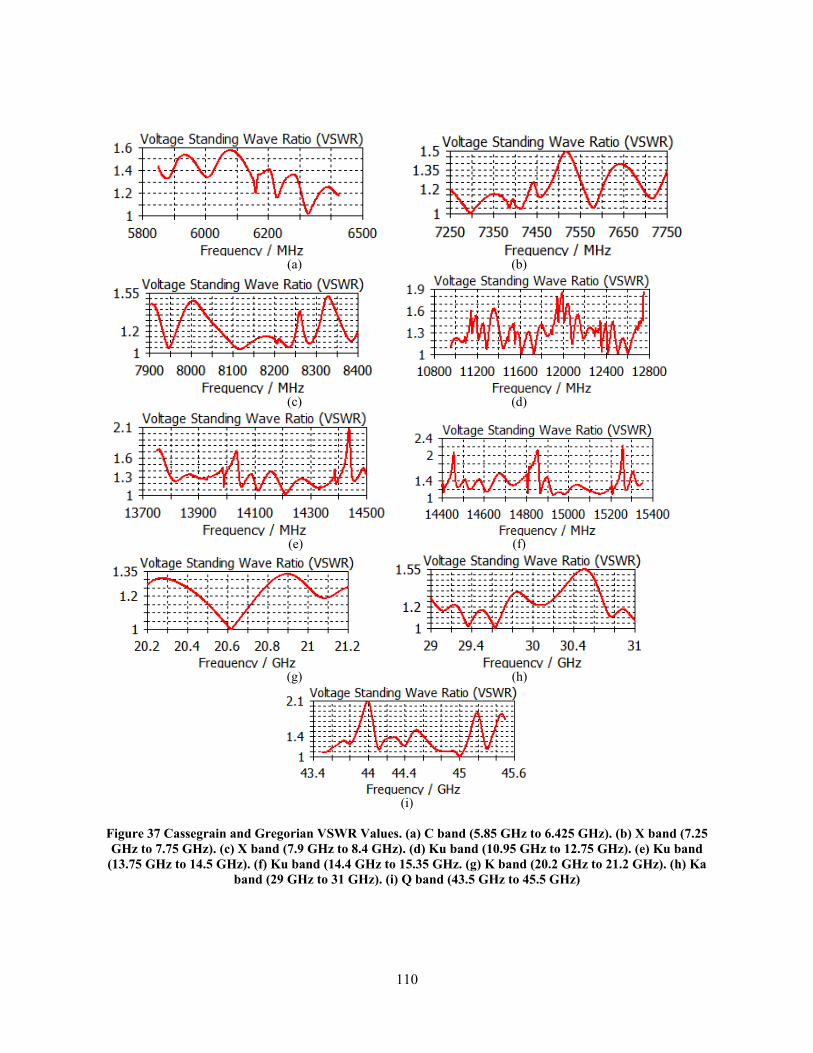
110

(a) (b)

(c) (d)

(e) (f)

(g) (h)

(i)

Figure 37 Cassegrain and Gregorian VSWR Values. (a) C band (5.85 GHz to 6.425 GHz). (b) X band (7.25

GHz to 7.75 GHz). (c) X band (7.9 GHz to 8.4 GHz). (d) Ku band (10.95 GHz to 12.75 GHz). (e) Ku band

(13.75 GHz to 14.5 GHz). (f) Ku band (14.4 GHz to 15.35 GHz. (g) K band (20.2 GHz to 21.2 GHz). (h) Ka

band (29 GHz to 31 GHz). (i) Q band (43.5 GHz to 45.5 GHz)

111

Radiation patterns, gain, side lobe levels and angular width (3 dB) were captured through

simulation using CST microwave studio. Figure 38 (a) through (i) depicts the frequency band

results for the C, X, Ku, K, Ka and Q band frequency range. The C band center frequency of 6.14

GHz had a gain of 36 dB with an angular width (3 dB) of 2 degrees and a side lobe level of -14.1

dB. The X band center frequency of 7.5 GHz had a gain of 36.6 dB with an angular width (3 dB)

of 1.1 degrees and a side lobe level of -11.7 dB. The X band center frequency of 8.15 GHz had a

gain of 39.2 dB with an angular width (3 dB) of 1.2 degrees and a side lobe level of -15.1 dB. The

Ku band center frequency of 11.9 GHz had a gain of 40.9 GHz with an angular width (3 dB) of

0.6 degrees and a side lobe level of -26.3 dB. The Ku band center frequency of 14.1 GHz had a

gain of 39.3 dB with an angular width (3 dB) of 0.3 degrees and a side lobe level of -13.1 dB. The

Ku band center frequency of 14.875 GHz had a gain of 40.1 dB with an angular width (3 dB) of

0.4 degrees and a side lobe level of -12 dB. The K band center frequency of 20.7 GHz had a gain

of 33.4 GHz with an angular width (3 dB) of 2.8 degrees and a side lobe level of -15.5 dB. The

Ka band center frequency of 30 GHz had a gain of 36.8 dB with an angular width (3 dB) of 2.1

degrees and a side lobe level -14.7 dB. The Q band center frequency of 44.5 GHz had a gain of

39.1 dB with an angular width (3 dB) of 1 degree and a side lobe level of -29.4 dB. These

frequencies represented the operating frequencies that the NMT Q / Ka, NMT X / Ka, directional

SDT and a limited set of operating frequencies of the CBSP antenna variants operated within.

(a) (b)

112

(c) (d)

(e) (f)

(g) (h)

(i)

Figure 38 Radiation Pattern for the Cassegrain and Gregorian Parabolic Stacked Antenna. (a) C band (6.14

GHz). (b) X band (7.5 GHz). (c) X band (8.15 GHz). (d) Ku band (11.9 GHz). (e) Ku band (14.1 GHz). (f) Ku

band (14.875 GHz). (g) K band (20.7 GHz). (h) Ka band (30 GHz). (i) Q band (44.5 GHz)

113

4.2 Gregorian with Splash Plate Antenna

The Gregorian with splash plate antenna operates within the frequency range of the NMT

Q / Ka, NMT X / Ka and SDT antennas. Additionally, this configuration allows for other

frequencies that the CBSP variants operate within except for the L band frequency range (.95 GHz

to 2.05 GHz) and the C band frequency range (3.7 GHz to 4.2 GHz). Utilizing the blockage area

that the Gregorian antenna produces, the splash plate antenna is able to be stacked in front of the

Gregorian antenna’s secondary reflector. The geometry of the Gregorian and splash plate antenna

is shown in Figure 39.

Figure 39 Gregorian and Splash Plate Stacked Antenna Geometric Properties

The splash plate antenna feed is a self-supported hat-fed system with a sub-reflector

attached with the shape of an axially displaced ellipsoid [99]. A displaced axis Gregorian antenna

with a single offset has geometric properties that the main reflector is parabolic while the sub-

reflector is a portion of an ellipse [100]. 𝐿𝑚𝑆 is the distance between the back of the main reflector

and the focus while 𝐿𝑠𝑆 is the distance between the focus and the edge of the sub-reflector. 𝐹𝑆 is

114

the focal distance of the main reflector, 𝐷𝑚𝑆 is the diameter of the main splash plate reflector, 𝐷𝑆𝑆

is the diameter of the splash plate sub-reflector, and 𝜃𝑒𝑆 is the angle between the Z axis and the

ray emanating from the focus [100]. Equation (17) depicts the distance between the back of the

main reflector and the focus with relationship between the splash plate main reflector dish and

splash plate sub-reflector.

𝑳𝒎𝑺 = 𝑭𝑺𝑫𝒎𝑺𝑫𝒎𝑺−𝑫𝑺𝑺 − 𝑫𝑺𝑺𝟒 (𝐜𝐨𝐬𝜽𝒆𝑺+𝟏𝐬𝐢𝐧𝜽𝒆𝑺 ) (17)

Equation (18) displays the distance between the edge of the splash plate sub-reflector and the

focus.

𝑳𝒔𝑺 = 𝟐𝐜𝐨𝐬Φ ( 𝑫𝑺𝑺𝟒 𝐬𝐢𝐧Φ) + 𝑫𝒔𝑺𝟐 𝐭𝐚𝐧𝝋 (18) Φ is the angle from the axis of the main splash plate reflector coordinate system to the top edge of

the main splash plate reflector as shown

𝐭𝐚𝐧Φ = 𝟐𝐜𝐨𝐬𝜽𝒆𝑺+𝟏𝐬𝐢𝐧 𝜽𝒆𝑺 − 𝟒𝑭𝑺𝑫𝒎𝑺−𝑫𝑺𝑺 (19)

𝜑 is the offset angle of the main splash plate reflector coordinate system and the splash plate sub-

reflector coordinate system as shown

𝐭𝐚𝐧𝝋 = 𝟖𝑭𝑺(𝑫𝒎𝑺−𝑫𝑺𝑺) (𝑫𝒎𝑺−𝑫𝑺𝑺)𝟐−𝟏𝟔𝑭𝑺𝟐 (20)

Using equation (19), the diameter of the splash plate sub-reflector with relation to the main splash

plate reflector is shown as

115

𝑫𝑺𝑺 = 𝑫𝒎𝑺 − 𝟒𝑭𝑺 𝐭𝐚𝐧Φ𝐭𝐚𝐧Φ(𝐜𝐨𝐬𝜽𝒆𝑺+𝟏𝐬𝐢𝐧𝜽𝒆𝑺 )−𝟐 (21)

The splash plate antenna is smaller than the sub-reflector of the larger Gregorian antenna

and is mounted in front while utilizing the blockage area that the sub-reflector produces. The feed

from the splash plate antenna is routed behind the splash plate antenna’s main parabolic dish, along

the front of the larger Gregorian sub-reflector and through the rear of the larger Gregorian’s main

parabolic dish. The side view and top view of the Gregorian and splash plate parabolic stacked

antenna is shown in Figure 40.

(a)

(b)

Figure 40 Gregorian and Splash Plate Parabolic Stacked Antenna. (a) Side View. (b) Top View

The Gregorian and splash plate parabolic stacked antenna had a Gregorian antenna with a

primary dish size of 1.5 m and a splash plate antenna stacked in front of the reflecting dish with a

primary dish size of 325.9 mm. The diameter of the Gregorian antenna is slightly smaller than the

116

NMT Q / Ka antenna that is currently fielded. Antenna Magus software was used to obtain the

physical parameters of each antenna and CST Microwave studio software integrated these two

antennas in a parabolic stack configuration. The physical parameter of the Gregorian and splash

plate parabolic stacked antenna is shown in Table 19 and Table 20.

Table 19 Physical Parameters of the Gregorian Antenna of the Parabolic Stacked Antenna

Description Short Name Value

Primary reflector diameter Dp 1.5 m

Primary reflector focal length Fp 443.6 mm

Secondary reflector diameter Ds 447.3 mm

Secondary reflector focal length Fs 354.9 mm Horn aperture to focal point offset Sf

0 m

Waveguide length Lg 36.78 mm

Flare length Lf 127 mm

Aperture height Ha 53.38 mm

Aperture width Wa 73.62 mm

Waveguide height Hg 14.44 mm

Waveguide width Wg 28.88 mm

Table 20 Physical Parameters of the Splash Plate Antenna of the Parabolic Stacked Antenna

Description Short Name Value

Dish diameter D 325.9 mm

Focal depth F 97.76 mm

Feed offset from focal point S 5.314 mm

Waveguide diameter Dg 10.02 mm

Waveguide length Lg 30.05 mm

Length of tuning roller Ltr 10.27 mm

Diameter of tuning roller Dtr 3.706 mm

Radius of dielectric lens Rdl 32.06 mm

Offset of dielectric lens Sdl 30.55 mm

Height of dielectric lens Hdl 11.02 mm

Diameter of reflecting plane Drp 54.09 mm

Diameter of spherical cap Dsc 12.02 mm

117

Height of spherical cap Hsc 1.503 mm

Inset / extension of dielectric into waveguide Sd 11.02 mm

The VSWR values for this configuration displayed results that were under the 2:1 VSWR

value. This parabolic stacked antenna configuration was capable of operating within frequency

bands C, X, Ku, K, Ka, and Q. The results depict operational capability to function within

frequencies corresponding to current capabilities of the NMT Q / Ka, NMT X / Ka, SDT and

certain frequencies that the CBSP antenna variants are capable of. The Gregorian antenna was

capable of operating within the C, X and Ku bands while the splash plate antenna was capable of

operating within the K, Ka, and Q bands. The maximum VSWR that was observed was within the

Ka band frequency range of 1.85:1. The VSWR values shown in Figure 41 (a)-(f) represented the

large Gregorian antenna values while the VSWR values shown in Figure 41 (g)-(i) were the results

of the small splash plate antenna.

(a) (b)

(c) (d)

(e) (f)

118

(g) (h)

(i)

Figure 41 Gregorian and Splash Plate VSWR Values. (a) C band (5.85 GHz to 6.425 GHz). (b) X band (7.25

GHz to 7.75 GHz). (c) X band (7.9 GHz to 8.4 GHz). (d) Ku band (10.95 GHz to 12.75 GHz). (e) Ku band

(13.75 GHz to 14.5 GHz). (f) Ku band (14.4 GHz to 15.35 GHz). (g) K band (20.2 GHz to 21.2 GHz). (h) Ka

band (29 GHz to 31 GHz). (i) Q band (43.5 GHz to 45.5 GHz)

Radiation patterns, gain values and side lobe levels for the C, X, Ku, K, Ka, and Q

frequency bands were captured for the Gregorian splash plate parabolic stacked antenna. The C

band center frequency of 6.14 GHz was used to depict a gain of 35.7 dB, side lobe level of -8.9

dB and an angular width (3 dB) of 1.4 degrees. The X band center frequency of 7.5 GHz was

simulated to obtain results of a gain value of 37.2 dB, side lobe level of -11.1 dB and an angular

width (3 dB) of 1.3 degrees. Center frequency 8.15 GHz which is also within the X band frequency

range produced results of 39.8 dB of gain, side lobe level of -24.9 dB and an angular width (3 dB)

of 1.0 degrees. Ku band center frequency 11.9 GHz demonstrated a gain value of 41 dB, side lobe

level of -26.7 dB and an angular width (3 dB) of 0.5 degrees. The Ku band center frequency of

14.1 GHz produced a gain of 41.6 GHz, side lobe level of -22.9 dB and an angular width (3 dB)

of 0.4 degrees. The LoS Ku band center frequency of 14.875 GHz had a gain of 34.6 dB, side lobe

level of -12.1 dB and an angular width (3 dB) of 2.9 degrees. Figure 42 (a)-(f) displayed gain and

radiation patterns of the large Gregorian antenna of this parabolic stacked antenna configuration.

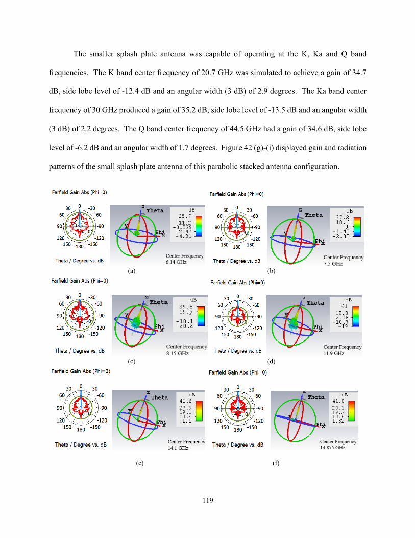
119

The smaller splash plate antenna was capable of operating at the K, Ka and Q band

frequencies. The K band center frequency of 20.7 GHz was simulated to achieve a gain of 34.7

dB, side lobe level of -12.4 dB and an angular width (3 dB) of 2.9 degrees. The Ka band center

frequency of 30 GHz produced a gain of 35.2 dB, side lobe level of -13.5 dB and an angular width

(3 dB) of 2.2 degrees. The Q band center frequency of 44.5 GHz had a gain of 34.6 dB, side lobe

level of -6.2 dB and an angular width of 1.7 degrees. Figure 42 (g)-(i) displayed gain and radiation

patterns of the small splash plate antenna of this parabolic stacked antenna configuration.

(a) (b)

(c) (d)

(e) (f)

120

(g) (h)

(i)

Figure 42 Radiation Pattern for the Gregorian and Splash Plate Parabolic Stacked Antenna. (a) C band (6.14

GHz). (b) X band (7.5 GHz). (c) X band (8.15 GHz). (d) Ku band (11.9 GHz). (e) Ku band (14.1 GHz). (f) Ku

band (14.875 GHz). (g) K band (20.7 GHz). (h) Ka band (30 GHz). (i) Q band (44.5 GHz)

The Gregorian and splash plate parabolic stacked antenna was similar in size to the

diameter of the NMT Q / Ka antenna of 1.5m. Capable frequencies ranged from frequency bands

C, X, Ku, K, Ka and Q. The Gregorian antenna was able to operate within frequency bands C, X

and Ku while the smaller splash plate antenna which had a diameter of 325.9mm operated at K,

Ka and Q band frequencies. VSWR values peaked at 1.85:1 within the Ka band frequency range

while gain values peaked within the Ku band frequency range at 41.8 dB. Considerations for this

parabolic stacked antenna configuration included being able to have a similar size to the NMT Q

/ Ka antenna in order to replace the currently fielded antenna at the end of its system life cycle.

The Gregorian and splash plate parabolic stacked antenna configuration was capable of operating

at frequencies equivalent to the NMT Q / Ka, NMT X / Ka and the directional portion of the SDT

antenna along with a portion of frequencies that the CBSP variants currently operate within.

121

4.3 Dual Gregorian Parabolic Stacked Antenna

A dual Gregorian parabolic stacked antenna provides capabilities that both NMT Q / Ka

and NMT X / Ka antennas operate within [101]. In addition to the NMT antennas variants, the

SDT directional antenna and certain frequencies that the CBSP antenna variants operate within are

also capable with this parabolic antenna stacking configuration. This parabolic stacking

configuration provides operation modes within the C, X, Ku, K, Ka, and Q band frequency range.

The C, X and Ku band frequencies are met with the larger dish within this configuration while the

smaller dish supports the K, Ka and Q band frequency ranges. The side view [101] and top view

of the dual Gregorian parabolic stacked antenna is shown in Figure 43.

(a)

(b)

Figure 43 Dual Gregorian Parabolic Stacked Antenna. (a) Side View [101]. (b) Top View

The dual Gregorian parabolic stacked antenna had a large parabolic dish of 1.921m and a

medium parabolic dish of 480mm. The larger Gregorian antenna had a dish diameter of 1.921m

with a sub-reflector size of 480mm which is 20% smaller than the fielded large NMT X / Ka

122

antenna. These antennas were stacked in front of one another utilizing the blockage space created

by the larger antenna’s secondary reflector. Antenna Magus software was used to obtain the

physical parameters of each Gregorian antenna to simulate within CST Microwave studio in a

parabolic stacked configuration. The physical parameters of the dual Gregorian parabolic stacked

antenna is shown in Table 21.

Table 21 Dual Gregorian Parabolic Stacked Antenna Physical Parameters

Gregorian Parabolic Stacked Antenna Physical Description

Short Name

Large Gregorian Antenna Values

Medium Gregorian Antenna Values

Primary reflector diameter Dp 1.921 m 480 mm

Primary reflector focal length Fp 504.8 mm 132.1 mm

Secondary reflector diameter Ds 480.2 mm 125.7 mm

Secondary reflector focal length Fs 403.8 mm 105.7 mm

Secondary reflector eccentricity Es 0.5604 0.5604

Horn aperture to focal point offset Sf 0 m 0 m

Waveguide length Lg 39.97 mm 9.993 mm

Flare length Lf 138.0 mm 34.50 mm

Aperture height Ha 58.00 mm 14.50 mm

Aperture width Wa 80.00 mm 20.00 mm

Waveguide height Hg 15.69 mm 3.922 mm

Waveguide width Wg 31.38 mm 7.845 mm

VSWR values that operate within the NMT Q / Ka and NMT X / Ka frequency ranges

were assessed. The VSWR values for this configuration displayed results that were under the 2:1

VSWR value with a maximum VSWR value of 1.68:1. The VSWR values for the X band

frequency range 7.25 GHz to 7.75 GHz displayed values ranging up to 1.5:1. Similar results

were shown for X band frequencies 7.9 GHz to 8.4 GHz with values ranging up to 1.49:1. K

band frequencies 20.2 GHz to 21.2 GHz depicted VSWR results of up to 1.48:1. Frequencies 29

GHz to 31GHz which reside on the Ka band had VSWR values up to 1.45:1. The Q band

123

frequency range of 43.5 GHz GHz to 45.5 GHz had VSWR values up to 1.68:1. VSWR values

for the triple Gregorian parabolic stacked antenna are shown in Figure 44.

(a) (b)

(c) (d)

(e)

Figure 44 VSWR of the Gregorian Parabolic Stacked Antenna. (a) X band (7.25 GHz – 7.75 GHz). (b) X band

(7.9 GHz – 8.4 GHz). (c) K band (20.2 GHz – 21.2 GHz). (d) Ka band (29 GHz – 31 GHz). (e) Q band (43.5 –

45.5 GHz)

Radiation patterns, gain values and side lobe levels for the X, K, Ka and Q frequency bands

which the NMT Q / Ka and NMT X / Ka variant antennas operate within were captured for the

dual Gregorian parabolic stacked antenna. The X band center frequency of 7.5 GHz was used to

depict a gain of 40 dB, side lobe level of -24.1 dB and an angular width (3 dB) of 0.8 degrees.

Center frequency 8.15 GHz which is also within the X band frequency range produced results of

41.5 dB of gain, side lobe level of -30 dB and an angular width (3 dB) of 0.7 degrees. K band

center frequency of 20.7 GHz was simulated to produce values of 36.1 dB of gain, side lobe level

of -14.1 dB and an angular width (3 dB) of 1.7 degrees. Ka band center frequency of 30 GHz

124

produced results of 40.8 dB of gain, side lobe level of -24.9 dB and an angular width (3 dB) of 0.6

degrees. The Q band center frequency of 44.5 GHz resulted in the gain value of 42.5 dB. This Q

band center frequency produced a side lobe level of -13.5 dB and an angular width (3 dB) of 3.7

degrees. Radiation patterns, gain values, and side lobe levels for these frequencies are shown in

Figure 45 (a)-(e).

(a) (b)

(c) (d)

(e)

Figure 45 Radiation patterns of the Gregorian parabolic stacked antenna. (a) X band (7.5 GHz). (b) X band

(8.15 GHz). (c) K band (20.7 GHz). (d) Ka band (30 GHz). (e) Q band (44.5 GHz)

125

The larger Gregorian antenna of the dual Gregorian parabolic stacked antenna

configuration was also capable of operating within limited CBSP antenna and the directional SDT

antenna variant frequency ranges. C band frequency range of 5.85 GHz to 6.425 GHz and Ku

band frequency ranges of 10.95 GHz to 12.75 GHz, 13.75 GHz to 14.5 GHz and 14.4 GHz to 15.35

GHz were simulated to obtain VSWR, radiation pattern, gain, side lobe level (3 dB) and angular

width results. The 5.85 GHz to 6.425 GHz CBSP frequency range is used for transmitting purposes

for CBSP operations. The Ku band 10.95 GHz to 12.8 GHz range is used for receiving purposes

while the 13.75 GHz to 14.5 GHz range is used to transmit. The SDT directional antenna uses the

Ku band frequency range of 14.4 GHz to 15.35 GHz for LoS transmit and receive functions. The

VSWR values for the C and Ku band frequency ranges were able to operate below the VSWR

value of 1.58:1 as shown in Figure 46 (a)-(d).

(a) (b)

(c) (d) Figure 46 VSWR of the Gregorian parabolic stacked antenna. (a) C band (5.8 GHz – 6.5 GHz). (b) Ku band

(10.8 GHz – 12.8 GHz). (c) Ku band (13.75 GHz – 14.5 GHz). (d) Ku band (14.4 GHz – 15.35 GHz)

Radiation patterns, gain values and side lobe levels for the C and Ku frequency bands were

captured for the dual Gregorian parabolic stacked antenna. The C band center frequency of 6.14

126

GHz was used to depict a gain of 38.4 dB, side lobe level of -15.6 dB and an angular width (3 dB)

of 1.4 degrees. Ku band center frequency of 11.9 GHz was simulated to produce values of 42.4

dB of gain, side lobe level of -23 dB and an angular width (3 dB) of 0.5 degrees. The Ku band

center frequency of 14.1 GHz provided simulation results of 42.4 dB of gain, side lobe level of -

29.3 dB and an angular width (3 dB) of 0.7 degrees. The Ku band center frequency of 14.875 GHz

depicted a gain of 42.3 dB, side lobe level of -22.3 dB and an angular width (3 dB) of 0.4 degrees.

Radiation patterns, gain values, and side lobe levels for certain CBSP frequencies as well as the

directional SDT antenna capability are shown in Figure 47 (a)-(d).

(a) (b)

(c) (d)

Figure 47 Radiation patterns of the Gregorian parabolic stacked antenna. (a) C band (6.14 GHz). (b) Ku

band (11.9 GHz). (c) Ku band (14.1 GHz). (d) Ku band (14.875 GHz)

127

The dual Gregorian parabolic stacked antenna contained two Gregorian antennas stacked

in front of one another to operate at the C, X, Ku, K, Ka and Q band frequencies. Results shown

gain values of that peaked at 42.5 dB at the Q band frequency range. Overall VSWR values were

under 2:1 with a maximum VSWR peaking at 1.68:1. This parabolic stacked antenna had

additional C and Ku band capabilities that the CBSP antenna provided as well as the directional

SDT LoS operating frequency range. The dual Gregorian parabolic stacked antenna is an efficient

solution for consolidating the NMT Q / Ka, NMT X / Ka and directional SDT antenna variants.

4.4 Dual Cassegrain with Splash Plate Parabolic Stacked Antenna

An improvement need was presented to field tri-band antennas (Q, Ka, X) to reduce topside

volume and antenna count [102]. The need for a tri-band antenna was referencing the NMT Q /

Ka and X / Ka antennas. Having a singular antenna that can operate at Q, Ka, and X band

frequencies would eliminate the need for two different NMT variant antennas. A tri-band

parabolic stacked antenna was focused on providing a Q, Ka and X band capable solution on a

single antenna pedestal [103]. This tri-band parabolic stacked antenna consisted of two Cassegrain

antennas and a splash plate antenna to operate within the Q, K, Ka and X band frequencies. This

parabolic stacked antenna had three antennas on a single pedestal to provide multiband frequency

capabilities. Additional frequency operation simulation testing revealed that this parabolic stacked

antenna configuration was capable of operating at frequencies that partially operate within CBSP

antenna operating frequencies as well as the directional SDT antenna frequency range. For NMT

Q / Ka and X / Ka frequency functionality, the large Cassegrain antenna provided the X band

frequency, the medium Cassegrain antenna provided K and Ka band frequencies, and the small

splash plate antenna provided the Q band frequency. As shown in Figure 48, the large Cassegrain

antenna, medium Cassegrain antenna and small splash plate antenna are stacked in front of one

128

another to provide C, X, Ku, K, Ka and Q band capabilities that the NMT Q / Ka, NMT X / Ka,

directional SDT antenna variants operate within as well as a portion of frequencies that the CBSP

antenna variants operate within.

(a)

(b)

Figure 48 Dual Cassegrain with Splash Plate Parabolic Stacked Antenna (a) Side view (b) Top view [103]

The overall antenna size of the dual Cassegrain with splash plate parabolic stacked antenna

was 36.8% smaller than the currently fielded NMT Q / Ka antenna. Utilizing a similar pedestal as

the NMT Q / Ka antenna would allow the currently fielded antenna to be replaced with the tri-

band parabolic stacked antenna with ease. The physical parameters for the tri-band parabolic

stacked antenna is shown in Table 22 and in Table 23.

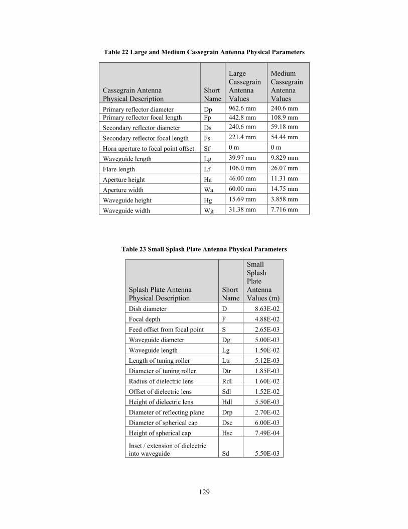
129

Table 22 Large and Medium Cassegrain Antenna Physical Parameters

Cassegrain Antenna Physical Description

Short Name

Large Cassegrain Antenna Values

Medium Cassegrain Antenna Values

Primary reflector diameter Dp 962.6 mm 240.6 mm

Primary reflector focal length Fp 442.8 mm 108.9 mm

Secondary reflector diameter Ds 240.6 mm 59.18 mm

Secondary reflector focal length Fs 221.4 mm 54.44 mm

Horn aperture to focal point offset Sf 0 m 0 m

Waveguide length Lg 39.97 mm 9.829 mm

Flare length Lf 106.0 mm 26.07 mm

Aperture height Ha 46.00 mm 11.31 mm

Aperture width Wa 60.00 mm 14.75 mm

Waveguide height Hg 15.69 mm 3.858 mm

Waveguide width Wg 31.38 mm 7.716 mm

Table 23 Small Splash Plate Antenna Physical Parameters

Splash Plate Antenna Physical Description

Short Name

Small Splash Plate Antenna Values (m)

Dish diameter D 8.63E-02

Focal depth F 4.88E-02

Feed offset from focal point S 2.65E-03

Waveguide diameter Dg 5.00E-03

Waveguide length Lg 1.50E-02

Length of tuning roller Ltr 5.12E-03

Diameter of tuning roller Dtr 1.85E-03

Radius of dielectric lens Rdl 1.60E-02

Offset of dielectric lens Sdl 1.52E-02

Height of dielectric lens Hdl 5.50E-03

Diameter of reflecting plane Drp 2.70E-02

Diameter of spherical cap Dsc 6.00E-03

Height of spherical cap Hsc 7.49E-04

Inset / extension of dielectric into waveguide Sd 5.50E-03

130

The Cassegrain antennas and the splash plate antenna combined provided the same RF

band capabilities that the NMT Q / Ka and NMT X / Ka antennas operate within. VSWR values

were assessed for frequencies within the X, K, Ka and Q bands. When no power is reflected from

the antenna, the VSWR value would be 1. For antenna design, the VSWR values are kept as low

as possible. The tri-band parabolic stacked antenna had VSWR values greater than 2:1 for

frequencies between 7.54 GHz through 7.71 GHz where the maximum VSWR value was 3.5:1

within the X band frequency range. The X band frequency range also had VSWR values greater

than 2:1 within the frequency range of 7.9 GHz through 8.07 GHz along with frequencies 8.36

GHz through 8.38 GHz. The K band frequency range had a maximum VSWR values of 1.73:1.

The Ka band frequency range had VSWR values greater than 2:1 between frequencies 30.1 GHz

and 30.35 GHz with the highest VSWR value being 2.4:1. The Q band frequency range had a few

ranges of frequencies that exceeded the VSWR value of 2:1 which included frequencies 44.8 GHz

to 45.5 GHz with the highest VSWR value being 2.28:1. The VSWR values with relationships to

the NMT Q / Ka and NMT X / Ka antenna variant frequencies are shown in Figure 49.

(a) (b)

(c) (d)

131

(e)

Figure 49 VSWR of the Dual Cassegrain and Splash Plate Parabolic Stacked Antenna. (a) X band (7.25 GHz -

7.75 GHz). (b) X band (7.9 GHz - 8.4 GHz). (c) K band (20.2 GHz to 21.2 GHz). (d) Ka band (29 GHz - 31

GHz). (e) Q band (43.5 GHz – 45.5 GHz) [103]

The dual Cassegrain and splash plate antenna had gain values of up to 34.6 dB for operating

frequencies related to the NMT Q / Ka and NMT X / Ka variant antennas. The X band which

operated within the large Cassegrain antenna had gain values of 34.4 dB at the center frequency

of 7.5 GHz and 34.6 dB at the center frequency of 8.15 GHz. The angular width (3 dB) was

measured at 2.5 degrees at the center frequency of 7.5 GHz and 2.6 degrees at the center frequency

of 8.15 GHz. The X band frequency simulated had side lobe level values of -14.1 dB at a center

frequency of 7.5 GHz and a side lobe level value of -26.2 dB for a center frequency of 8.15 GHz.

The K band center frequency of 20.7 had a gain of 29.4 dB with a side lobe level -1.1 dB and an

angular width (3 dB) of 39.9 degrees which operated within the medium Cassegrain antenna. The

medium Cassegrain antenna had a 34.4 dB gain value when simulated using the Ka band center

frequency 30 GHz. The medium Cassegrain antenna had an angular width (3 dB) of 2.4 degrees

with a side lobe level of -13.2 GHz utilizing the 30 GHz center frequency. The small splash plate

antenna had a 26.3 dB gain at Q band center frequency 44.5 GHz. This small splash plate antenna

depicted a side lobe level of -12.5 dB with an angular width (3 dB) of 4.3 degrees. The radiation

patterns for the dual Cassegrain and splash plate parabolic stacked antenna is shown in Figure 50.

132

(a) (b)

(c) (d)

(e)

Figure 50 Radiation pattern of the Dual Cassegrain and Splash Plate Parabolic Stacked Antenna. (a) X band

(7.5 GHz). (b) X band (8.15 GHz). (c) K band (20.7 GHz). (d) Ka band (30 GHz). (e) Q band (44.5 GHz) [103]

The dual Cassegrain and splash plate parabolic stacked antenna was capable of operating

within some of the CBSP operating frequencies for SATCOM communications and the SDT

operating frequencies for LoS communications. The C band frequency range of 5.85 GHz to 6.425

GHz had VSWR values that peaked to 3.4:1. Frequencies 5.92 GHz to 6.425 GHz had VSWR

values less than 2.4:1. The Ku band frequency range of 10.95 GHz to 12.175 GHz had VSWR

values equal and less than 2.6:1. The Ku band frequency range of 13.75 GHz to 14.5 GHz had

VSWR values equal and less than 2.65. The LoS Ku band frequency range of 14.4 to 15.35 GHz

133

has VSWR values equal and less than 2.8:1. This antenna was not capable of operating within the

L band frequency range of .95 GHz to 2.05 GHz and the lower C band frequency range of 3.7 GHz

to 4.2 GHz. The VSWR values for the capable frequencies are shown in Figure 51 (a)-(d).

(a) (b)

(c) (d)

Figure 51 VSWR of the dual Cassegrain and splash plate parabolic stacked antenna. (a) C band (5.85 GHz to

6.425 GHz). (b) Ku band (10.95 GHz to 12.75 GHz). (c) Ku band (13.75 GHz to 14.5 GHz). (d) Ku band (14.4

GHz to 15.35 GHz)

Radiation patterns, gain, side lobe levels, and angular width (3 dB) were captured using

the frequencies that the CBSP antenna and directional SDT antennas are capable of operating

within with the exception of the L band frequency range .95 GHz to 2.05 GHz and the lower C

band frequency range of 3.7 GHz to 4.2 GHz. The C band center frequency of 6.14 GHz was

simulated to obtain a gain of 31.8 dB, side lobe level of -13.1 dB and an angular width (3 dB) of

2.9 degrees. The Ku band center frequency of 11.9 GHz produced a gain of 34.5 dB, side lobe

level of -12.5 dB and an angular width (3 dB) of 2.5 degrees. The Ku band center frequency of

14.1 GHz was also simulated to obtain a gain value of 33.2 dB, side lobe level of -18.5 dB and an

angular width (3 dB) of 2.9 degrees. The LoS Ku band center frequency of 14.875 achieved a gain

value of 34.6 dB, side lobe level of -19.9 dB and an angular width (3 dB) of 2.7 degrees. Radiation

134

patterns for the frequencies tested that were capable of performing at limited CBSP antenna

operating frequencies and SDT directional antenna frequencies for the dual Cassegrain parabolic

stacked antenna are shown in Figure 52 (a)-(d).

(a) (b)

(c) (d)

Figure 52 Radiation pattern of the dual Cassegrain and splash plate parabolic stacked antenna. (a) C band

(6.14 GHz). (b) Ku band (11.9 GHz). (c) Ku band (14.1 GHz). (d) Ku band (14.875 GHz)

The dual Cassegrain with splash plate parabolic stacked antenna has the ability to meet the

RF band needs for consolidating the NMT Q / Ka, X / Ka and directional SDT antenna variants.

Consolidating three variants of antennas reduces the amount of space required along with

providing additional capability to smaller shipboard platforms that do not have the space to allow

multiple antenna variants to be placed topside. The parabolic stacked antenna methodology used

in this configuration combined two Cassegrain antennas and one splash plate antenna on a single

pedestal to provide X, K, Ka and Q band frequency capabilities along with limited CBSP antenna

and SDT antenna frequency capabilities operating within the C and Ku band.

135

4.5 Triple Cassegrain Parabolic Stacked Antenna

The triple Cassegrain parabolic stacked antenna is another configuration to support the

consolidation of the NMT Q / Ka, NMT X / Ka and directional SDT variant antennas. The

parabolic stacked antenna described features the directional capability of the CDL LoS antenna

only whereas the omni directional antenna feature would be best suited for a separate antenna that

can radiate in all directions equally [104]. The LoS operational feature lies within the Ku band

frequency range of 14.4 GHz – 15.35 GHz. This is an additional capability where this parabolic

stacked antenna can be used for both SATCOM and LoS operations. This configuration uses three

Cassegrain parabolic antennas stacked in front of one another to operate at the LoS and SATCOM

frequency bands. The side view and top view of the triple Cassegrain parabolic stacked antenna

is shown in Figure 53.

(a)

136

(b)

Figure 53 Triple Cassegrain Parabolic Stacked Antenna. (a) Side view. (b) Top view [104]

The triple Cassegrain parabolic stacked antenna had a large Cassegrain antenna with a 1.9m

parabolic dish, a medium Cassegrain antenna with a 480mm parabolic dish, and a small Cassegrain

antenna with a 125.7 mm parabolic dish. Each antenna was stacked in front of one another with

the feed being routed through the back side of each parabolic antenna to the rear of the large

Cassegrain antenna. Antenna Magus software was used to model the individual Cassegrain

antennas for CST Microwave Studio simulation and the physical parameters of the triple

Cassegrain parabolic stacked antenna is shown in Table 24.

Table 24 Triple Cassegrain Parabolic Stacked Antenna Physical Parameters

Triple Cassegrain Parabolic Stacked Antenna Physical Description

Short Name

Large Cassegrain Antenna Values

Medium Cassegrain Antenna Values

Small Cassegrain Antenna Values

Primary reflector diameter Dp 1.9 m 480 mm 125.7 mm

Primary reflector focal length Fp 609.8 mm 165.7 mm 42.86 mm

Secondary reflector diameter Ds 480.0 mm 125.7 mm 37.59 mm

Secondary reflector focal length Fs 304.9 mm 82.84 mm 21.43 mm Horn aperture to focal point offset Sf

0 m 0 m 0 m

Waveguide length Lg 39.97 mm 14.48 mm 6.662 mm

Flare length Lf 88.00 mm 31.88 mm 14.67 mm

Aperture height Ha 38.67 mm 14.01 mm 6.444 mm

Aperture width Wa 49.33 mm 17.87 mm 8.222 mm

137

Waveguide height Hg 15.69 mm 5.684 mm 2.615 mm

Waveguide width Wg 31.38 mm 11.37 mm 5.230 mm

The VSWR values for the triple Cassegrain parabolic stacked antenna resulted in VSWR

values of up to 2.58:1. The large Cassegrain antenna at X band frequency range of 7.25 GHz to

7.75 GHz had VSWR values reaching up to 1.52:1. The large Cassegrain antenna at the X band

frequency range of 7.9 GHz to 8.4 GHz had VSWR values up to 1.48:1. The large Cassegrain

antenna at the Ku band which provides the LoS capability had VSWR values of up to 1.55:1 which

spanned the frequencies of 14.4 GHz to 15.35 GHz. VSWR values of up to 1.54:1 were obtained

for the medium Cassegrain antenna at the K band frequency range of 20.2 GHz to 21.2 GHz. The

medium Cassegrain antenna at the Ka band frequency range of 29 GHz to 31 GHz had VSWR

values of up to 2.58:1. The small Cassegrain antenna at the Q band frequency range of 43.5 GHz

to 45.5 GHz had VSWR values up to 2:1. The VSWR values for the triple Cassegrain parabolic

stacked antenna capable of operating at frequencies that the NMT Q / Ka, NMT X / Ka and

directional SDT antenna variants are show in Figure 54 (a)-(f).

(a) (b)

(c) (d)

138

(e) (f)

Figure 54 VSWR of Triple Cassegrain Parabolic Stacked Antenna. (a) X band (7.25 GHz – 7.75 GHz). (b) X

band (7.9 GHz – 8.4 GHz). (c) Ku band (14.4 GHz – 15.35 GHz). (d) K band (20.2 GHz – 21.2 GHz). (e) Ka

band (29 GHz to 31 GHz). (f) Q band (33 GHz – 50 GHz). [104]

Radiation patterns, gain, side lobe levels and angular width (3 dB) values were obtained by

simulating the triple Cassegrain parabolic stacked antenna through CST microwave studio for

frequencies associated with the NMT Q / Ka, NMT X /Ka and directional SDT antenna variants.

Frequency bands X, Ku, K, Ka and Q were successfully captured for the triple Cassegrain parabolic

stacked antenna. The large Cassegrain antenna at X band center frequency of 7.5 GHz was used

to depict a gain of 40.6 dB, an angular width (3 dB) of 0.8 degrees and side lobe level of -28 dB.

The large Cassegrain antenna at X band center frequency 8.15 GHz produced results of 41.5 dB

of gain, angular width (3 dB) of 0.7 degrees and side lobe level of -22.9 dB. The large Cassegrain

antenna at Ku band center frequency of 14.875 GHz operated at 40.1 dB of gain, angular width (3

dB) of 0.6 degrees and a side lobe level of -22.6 dB. The medium Cassegrain antenna at K band

center frequency of 20.7 GHz was simulated to produce values of 37.4 dB of gain, angular width

(3 dB) of 1.8 degrees and side lobe level of -14.5 dB. The medium Cassegrain antenna at Ka band

center frequency of 30 GHz produced results of 40.3 dB of gain, angular width (3 dB) of 0.9

degrees and side lobe level of -28.2 dB. The small Cassegrain antenna at Q band center frequency

of 44.5 GHz resulted in the gain value of 32.5 dB. This Q band center frequency produced an

angular width (3 dB) of 3.4 degrees and side lobe level of -13.1 dB. Radiation patterns, gain

values, and side lobe levels for these frequencies are shown in Figure 55 (a)-(f).

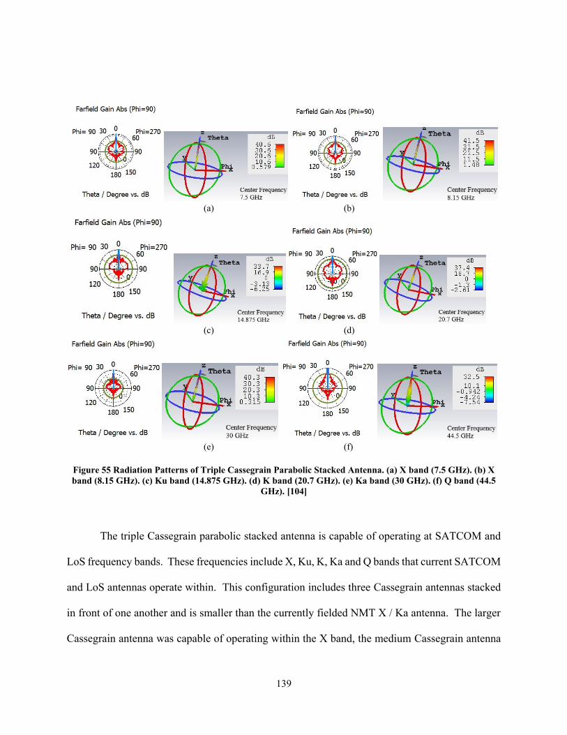
139

(a) (b)

(c) (d)

(e) (f)

Figure 55 Radiation Patterns of Triple Cassegrain Parabolic Stacked Antenna. (a) X band (7.5 GHz). (b) X

band (8.15 GHz). (c) Ku band (14.875 GHz). (d) K band (20.7 GHz). (e) Ka band (30 GHz). (f) Q band (44.5

GHz). [104]

The triple Cassegrain parabolic stacked antenna is capable of operating at SATCOM and

LoS frequency bands. These frequencies include X, Ku, K, Ka and Q bands that current SATCOM

and LoS antennas operate within. This configuration includes three Cassegrain antennas stacked

in front of one another and is smaller than the currently fielded NMT X / Ka antenna. The larger

Cassegrain antenna was capable of operating within the X band, the medium Cassegrain antenna

140

was capable of operating within the Ku, K and Ka bands, and the small Cassegrain antenna was

capable of operating within the Q band frequency range.

The triple Cassegrain antenna had additional capabilities of operating within certain

frequencies that the CBSP antenna variants provided with the exception of the L band (0.95 GHz

– 2.05 GHz) frequency range and the C band (3.7 GHz to 4.2 GHz) frequency range. This

parabolic stacked antenna configuration also had overlapping operating frequency capabilities

between the large, medium and small Cassegrain antennas. The large Cassegrain antenna was

capable of operating within the C band frequency range of 5.85 GHz to 6.425 GHz with a

maximum VSWR value of 1.81:1, gain of 38.3 dB, angular width (3 dB) of 1.1 degrees and a side

lobe level of -15.1 db. Figure 56 depicts the large Cassegrain C band VSWR and radiation details

of the triple Cassegrain parabolic stacked antenna configuration.

Figure 56 Large Cassegrain C Band VSWR and Radiation Details of the Triple Cassegrain Parabolic Stacked

Antenna Configuration

The large Cassegrain antenna was capable of operating within the Ku band frequency range

of 10.95 GHz to 12.75 GHz with a maximum VSWR value of 1.68:1, gain of 43.5 dB, angular

width (3 dB) of 0.4 degrees and a side lobe level of -29.8 db. This CBSP operating frequency is

141

used for receiving communication capabilities. Figure 57 depicts the large Cassegrain Ku band

VSWR and radiation details of the triple Cassegrain parabolic stacked antenna configuration.

Figure 57 Large Cassegrain Ku band VSWR and Radiation Details of the Triple Cassegrain Parabolic

Stacked Antenna Configuration

The large Cassegrain and medium Cassegrain antenna was capable of operating at the Ku

band frequency 13.75 GHz to 14.5 GHz. Figure 58(a) displays results for the large Cassegrain

antenna where the peak VSWR value was 1.84:1, 39.3 dB of gain, side lobe level of -22.7 dB and

an angular width (3 dB) of 0.5 degrees. Figure 58(b) depicts the results for the medium Cassegrain

antenna where the peak VSWR value was 2.1:1, 33.2 dB of gain, side lobe level of -13.7 dB and

an angular width (3 dB) of 2.5 degrees. The large Cassegrain antenna provided slightly lower

VSWR results and higher gain then the medium Cassegrain antenna. The larger Cassegrain

antenna is recommended to be used primarily with the medium Cassegrain antenna being used as

a backup.

142

(a)

(b) Figure 58 Ku band 13.75 GHz to 14.5 GHz VSWR and Radiation Details of the Triple Cassegrain Parabolic

Stacked Antenna Configuration Comparison. (a) Large Cassegrain Antenna Results. (b) Medium Cassegrain

Antenna Results

The large Cassegrain and medium Cassegrain antenna was capable of operating at the Ku

band frequency 14.4 GHz to 15.35 GHz. Figure 59(a) displays results for the large Cassegrain

antenna where the peak VSWR value was 1.55:1, 40.1 dB of gain, side lobe level of -22.6 dB and

an angular width (3 dB) of 0.6 degrees. Figure 59(b) depicts the results for the medium Cassegrain

antenna where the peak VSWR value was 1.81:1, 33.7 dB of gain, side lobe level of -14.3 dB and

an angular width (3 dB) of 2.4 degrees. The large Cassegrain antenna provided slightly lower

VSWR results and higher gain then the medium Cassegrain antenna. The larger Cassegrain

antenna is recommended to be used primarily with the medium Cassegrain antenna being used as

a backup.

143

(a)

(b)

Figure 59 Ku band 14.4 GHz to 15.4 GHz VSWR and Radiation Details of the Triple Cassegrain Parabolic

Stacked Antenna Configuration Comparison. (a) Large Cassegrain Antenna Results. (b) Medium Cassegrain

Antenna Results.

The medium Cassegrain and small Cassegrain antenna was capable of operating at the Ka

band frequency 29 GHz to 31 GHz. Figure 60(a) displays results for the medium Cassegrain

antenna where the peak VSWR value was 2.58:1, 40.3 dB of gain, side lobe level of -28.2dB and

an angular width (3 dB) of 0.9 degrees. Figure 60(b) depicts the results for the small Cassegrain

antenna where the peak VSWR value was 2.15:1, 28.2 dB of gain, side lobe level of -12.9 dB and

an angular width (3 dB) of 4.4 degrees. The medium Cassegrain antenna provided slightly higher

VSWR results and higher gain then the small Cassegrain antenna. The medium Cassegrain

antenna is recommended to be used primarily due to the high gain value with the small Cassegrain

antenna being used as a backup.

144

(a)

(b)

Figure 60 Ka band 29 GHz to 31 GHz VSWR and Radiation Details of the Triple Cassegrain Parabolic

Stacked Antenna Configuration Comparison. (a) Medium Cassegrain Antenna Results. (b) Small Cassegrain

Antenna Results

The medium Cassegrain and small Cassegrain antenna was capable of operating at the Q

band frequency 43.5 GHz to 45.5 GHz. Figure 61(a) displays results for the medium Cassegrain

antenna where the peak VSWR value was 2.35:1, 34.2 dB of gain, side lobe level of -16.4 dB and

an angular width (3 dB) of 3.4 degrees. Figure 61(b) depicts the results for the small Cassegrain

antenna where the peak VSWR value was 2:1, 32.5 dB of gain, side lobe level of -13.1 dB and an

angular width (3 dB) of 3.4 degrees. The medium Cassegrain antenna provided slightly higher

VSWR results and higher gain then the small Cassegrain antenna. The medium Cassegrain

antenna is recommended to be used primarily due to the high gain value with the small Cassegrain

antenna being used as a backup.

145

(a)

(b)

Figure 61 Q band 43.5 GHz to 44.5 GHz VSWR and Radiation Details of the Triple Cassegrain Parabolic

Stacked Antenna Configuration Comparison. (a) Medium Cassegrain Antenna Results. (b) Small Cassegrain

Antenna Results

The triple Cassegrain parabolic stacked antenna is capable of operating within C, X, Ku,

K, Ka and Q band frequencies. Operational capabilities include functioning within frequencies

that the NMT Q / Ka, NMT X / Ka and directional SDT antenna variants currently provide.

Operating frequencies that CBSP antenna variants provide are limited with the triple Cassegrain

parabolic stacked antenna configuration. Certain frequencies were capable of operating at a

particular sized antenna along with the next sized antenna stacked in front of it. This capability

provides redundancy with potential failover options for overall operational availability.

146

4.6 Dual Splash Plate Parabolic Stacked Antenna Assessment

To achieve multiband frequency capabilities, parabolic antenna stacking allows multiple

antennas to exist on a single pedestal. Reducing the amount of shipboard topside antennas assist

with decreasing the weight, space and power multiple platforms consume as well as promoting

system life cycle cost savings. Simulation testing was performed using CST Microwave Studio

with the assistance of Antenna Magus software. A dual splash plate parabolic stacked antenna is

capable of operating at frequencies within the L, C, Ku, K, Ka, X and Q bands. This parabolic

stacked antenna can consolidate CBSP FLV, CBSP ULV, NMT Q / Ka, NMT X / Ka, and

directional SDT antennas. The dual splash plate parabolic stacked antenna consists of a large

splash plate antenna which has a 2.248m diameter dish with an 810mm diameter reflecting plane

(drp) and smaller splash plate antenna that is comprised of a secondary 810mm diameter dish with

a 149mm drp. The dual splash plate parabolic stacked antenna model is shown in Figure 62.

Figure 62 Dual Splash Plate Parabolic Stacked Antenna [105]

The larger splash plate antenna is capable of operating at frequency bands L, C, Ku and X.

The smaller splash plate antenna is capable of operating at frequency bands X, Ku, K, Ka and Q.

147

The dual splash plate parabolic stacked antenna features capabilities of the CBSP, NMT and

directional SDT antenna variants. The smaller splash plate antenna is mounted in front of the

larger splash plate antenna. The smaller splash plate antenna’s wave guide would be routed around

the larger splash plate antenna’s drp and through the larger splash plate antenna’s parabolic dish.

A side view of the dual splash plate parabolic stacked antenna model is shown in Figure 63.

(a)

(b)

Figure 63 Side View of the Dual Splash Plate Parabolic Stacked Antenna. (a) Side View. (b) Top View [105]

The smaller splash plate antenna is mounted in front of the larger splash plate antenna. The

larger splash plate antenna had a diameter of 2.248 m for the primary parabolic dish. The drp of

the larger splash plate antenna had a diameter of 810 mm. To reduce the amount of physical

interference of the smaller splash plate antenna, the smaller splash plate antenna was designed to

have a primary parabolic dish of the same value as the drp of the larger splash plate antenna. The

148

smaller splash plate antenna had a diameter of 810 mm for the primary parabolic dish. The drp of

the smaller splash plate antenna had a diameter of 149 mm. The physical dimensions for the dual

splash plate parabolic stacked antenna are described in Table 25.

Table 25 Physical Dimensions of the Dual Splash Plate Parabolic Stacked Antenna

Splash Plate Antenna Physical Description

Short Name

Large Splash Plate Antenna Values (m)

Small Splash Plate Antenna Values (m)

Dish diameter D 2.25E+00 8.10E-01

Focal depth F 6.75E-01 2.48E-01

Feed offset from focal point S 7.33E-02 0.0135

Waveguide diameter Dg 1.38E-01 2.54E-02

Waveguide length Lg 4.15E-01 7.63E-02

Length of tuning roller Ltr 1.42E-01 2.61E-02

Diameter of tuning roller Dtr 5.11E-02 9.41E-03

Radius of dielectric lens Rdl 4.42E-01 8.14E-02

Offset of dielectric lens Sdl 4.22E-01 7.76E-02

Height of dielectric lens Hdl 1.52E-01 2.80E-02

Diameter of reflecting plane Drp 8.10E-01 1.49E-01

Diameter of spherical cap Dsc 1.66E-01 3.05E-02

Height of spherical cap Hsc 2.07E-02 3.82E-03

Inset / extension of dielectric into waveguide Sd 1.52E-01 2.80E-02

The 2.248m diameter dish with an 810mm drp and the secondary 810mm diameter dish

with a 149mm drp were simulated to observe the radiation pattern as well as identify VSWR, gain,

side lobe and angular width (3 dB) values. CST Microwave Studio simulation software was used

to assess the frequency ranges that these antennas were capable of operating in. The frequency

bands that were used for testing included L, C, X, Ku, K, Ka, and Q bands. The frequency bands

tested reflect the operational capabilities of the CBSP FLV / ULV, NMT Q / Ka, NMT X / Ka,

and directional SDT antenna variants. The (T) denotes the transmitting frequency while the (R)

149

denotes the receiving frequency. The (T) and (R) side by side represents that both transmitting

and receiving frequencies are operated within that range. There were instances where both the

larger and the smaller antenna were able to operate at a particular frequency range. The smaller

antenna had conflicts with operating at low frequency ranges while the larger antenna had conflicts

of operating at higher frequency ranges. The constraints for certain frequencies are shown in Table

26.

Table 26 Frequency to Parabolic Stacked Antenna Gain Relationship

CBSP FLV

(T)(R)

CBSP (R)

CBSP (T)

CBSP ULV & NMT (R)

CBSP ULV & NMT (T)

CBSP ULV (R)

CBSP ULV &

FLV (T)

SDT (T)(R)

NMT (R)

CBSP ULV & NMT (R)

NMT (T)(R)

950 to 2050 GHz

3.7 to 4.2

GHz

5.85 to 6.425 GHz

7.25 to 7.75 GHz

7.9 to 8.4

GHz

10.95 to 12.75 GHz

13.75 to 14.5 GHz

14.4 to 15.35 GHz

20.2 to 21.2 GHz

29 to 31 GHz

43.5 to 45.5 GHz

L Band

C Band

C Band

X Band

X Band

Ku Band

Ku Band

Ku Band

K Band

Ka Band

Q Band

Center Freq.

1.5 GHz

3.95 GHz

6.14 GHz

7.50 GHz

8.15 GHz

11.9 GHz

14.1 GHz

14.9 GHz

20.7 GHz

30 GHz

44.5 GHz

2248mm Dish 810mm DRP Gain

27.5 dB

25.8 dB

29.4 dB

24.6 dB

32 dB

36.2 dB

27.6 dB

32 dB 26

VSWR 3.2:1 2.8:1 3:1 3.4:1 4.4:1 3.7:1 2.58:1 2.3:1

810mm Dish 149mm DRP Gain 19.3 28.1 31.7

34 dB

34.2 dB

33.5 dB

31.5 dB

27.1 dB

34.1 dB

35.8 dB

41.6 dB

VSWR 4.5:1 1.75:1 3.1:1 2.05:1 2.25:1 2.9:1 3.6:1 2.05:1

=N/A

=Recommended antenna to use based on VSWR Values

VSWR values and radiation patterns were recorded amongst the 2.248m diameter dish

antenna with an 810mm drp and the secondary 810mm diameter dish antenna with a 149mm drp.

The simulation outputs were recorded to provide which antenna will operate more efficiently

150

utilizing the L, C, X, Ku, K, Ka, and Q frequency bands. This parabolic stacked antenna would

provide a method of consolidating the CBSP FLV, CBSP ULV, NMT X / Ka, NMT Q / Ka and

directional SDT antennas to a singular platform solution.

The 2.248m diameter dish with an 810mm drp was simulated using the L Band frequency

range 950 MHz to 2050 MHz shown in Figure 64. There were instances where frequencies within

the L Band range exceeded the targeted VSWR value 2:1. The center frequency (1500 MHz)

performed well with having a value less than 2:1. Frequencies between 1275 MHz and 1405 MHz

had VSWR values greater than 4:1, while frequencies after that range spanning to 2050 MHz

stayed below the VSWR value of 4:1. Frequencies between the 1405 MHz and 2050 MHz range

stayed around the VSWR value of 2:1 mark with a few deviations of +/- 1. The radiation pattern

depicts a main lobe magnitude of 27.5 db with an angular width (3 dB) of 5.4 degrees and a side

lobe level of -10.0 dB. The secondary splash plate antenna was unable to meet the capability of

supporting L band frequencies of 950 to 2050 MHz.

Figure 64 2.248m Splash Plate VSWR and Radiation Pattern for the L band Frequency 950 MHz to 2050

MHz

The 2.248m diameter dish with an 810mm drp was simulated using the C Band frequency

range 3700 MHz to 4200 MHz as shown in Figure 65. There were a few instances where

151

frequencies within the C Band range exceeded the targeted VSWR value 2:1. Frequencies 3725

MHz to 3780 MHz had VSWR values ranging from 2.1:1 to 2.8:1, and frequencies 4050 MHz to

4060 MHz had VSWR values ranging from 2.1:1 to 2.6:1. The center frequency (3950 MHz)

performed well with having a value less than 2:1. The radiation pattern depicts a main lobe

magnitude of 25.8 db with an angular width (3 dB) of 1.9 degrees and a side lobe level of -4.9 dB.

The secondary splash plate antenna was unable to meet the capability of supporting C band

frequencies of 3700 MHz to 4200 MHz.

Figure 65 2.248m Splash Plate VSWR and Radiation Pattern for the C band Frequency 3700 MHz to 4200

MHz

The 2.248m diameter dish with an 810mm drp was simulated using the C Band frequency

range 5850 MHz to 6425 MHz shown in Figure 66. There were a few instances where frequencies

within the C Band range exceeded the targeted VSWR value 2:1. Frequencies 5850 MHz to 5860

MHz had VSWR values ranging from 2.35:1 to 2.1:1, and frequencies 5875 MHz to 5885 MHz

had VSWR values ranging from 2.35:1 to 2.1:1 as well. Frequencies 5970 MHz and 5980 MHz

had VSWR values from 2.3:1 to 2.1:1. Frequencies 6075 MHz to 6100 had VSWR values ranging

from 2.1:1 to 2.42:1. Frequencies 6125 MHz to 6150 MHz had VSWR values ranging from 2.1:1

to 2.39:1. Frequencies 6310 MHz to 6360 MHz had VSWR values between 2.1:1 and 2.8:1.

Frequencies 6390 MHz to 6425 MHz had VSWR values between 2.1:1 and 3:1. The center

152

frequency (6140 MHz) performed well with having a value less than 2:1. The radiation pattern

depicts a main lobe magnitude of 29.4 dB with an angular width (3 dB) of 0.8 degrees and a side

lobe level of -2.1 dB. The secondary splash plate antenna was unable to meet the capability of

supporting C band frequencies of 5850 MHz to 6425 MHz.

Figure 66 2.248m Splash Plate VSWR and Radiation Pattern for the C band Frequency 5850 MHz to 6425

MHz

The 2.248m diameter dish with an 810mm drp and the secondary 810mm diameter dish

with a 149mm drp was simulated using the X Band frequency range 7250 MHz to 7750 MHz as

shown in Figure 67. There were a few instances where frequencies within the C Band range

exceeded the targeted VSWR value 2:1. Frequencies 7355 MHz to 7390 MHz had VSWR values

ranging from 2.1:1 to 2.9:1. Frequencies 7460 MHz to 7540 MHz had VSWR values between

2.1:1 and 3.4:1. Frequencies 7555 MHz to 7570 MHz had VSWR values ranging from 2.1:1 to

3.3:1. Frequencies 7725 MHz to 7750 MHz had VSWR values from 2.1:1 to 3:1. The center

frequency (7500 MHz) performed well with having a value slightly greater than 2:1. The radiation

pattern depicts a main lobe magnitude of 24.6 dB with an angular width (3 dB) of 2.7 degrees and

a side lobe level of -3.3 dB. The secondary splash plate antenna having an 810mm diameter dish

with an 149mm drp was able to operate at X band frequencies of 7250 to 7750 MHz, but had

153

VSWR values much greater than 2:1. VSWR values ranged from 4.5:1 to 2.5:1 and had a main

lobe magnitude of 34 dB. Due to the overall VSWR values, the larger 2.248m diameter dish with

an 810 drp is recommended for primary use.

(a)

(b)

Figure 67 Splash Plate VSWR and Radiation Pattern for the X band Frequency 7250 MHz to 7750 MHz. (a)

Large Splash Plate Results. (b) Small Splash Plate Results

The 2.248m diameter dish with an 810mm drp and the secondary 810mm diameter dish

with a 149mm drp was simulated using the X Band frequency range 7900 MHz to 8400 MHz as

shown in Figure 68. There were a few instances where frequencies within the X Band range

exceeded the targeted VSWR value 2:1. Frequencies 8055 MHz through 8100 MHz had VSWR

values ranging from 2.1:1 to 2.6:1. Frequencies 8140 MHz through 8145 MHz had VSWR values

ranging from 2.1:1 to 2.3:1. Frequencies 8160 MHz to 8165 MHz had VSWR values ranging from

2.1:1 to 2.2:1. Frequencies 8170 MHz to 8205 MHz had VSWR values of 2.1:1 to 4.4:1.

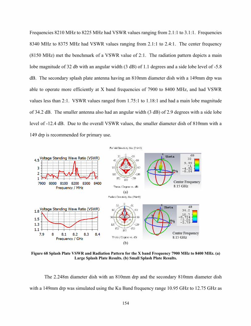
154

Frequencies 8210 MHz to 8225 MHz had VSWR values ranging from 2.1:1 to 3.1:1. Frequencies

8340 MHz to 8375 MHz had VSWR values ranging from 2.1:1 to 2.4:1. The center frequency

(8150 MHz) met the benchmark of a VSWR value of 2:1. The radiation pattern depicts a main

lobe magnitude of 32 db with an angular width (3 dB) of 1.1 degrees and a side lobe level of -5.8

dB. The secondary splash plate antenna having an 810mm diameter dish with a 149mm drp was

able to operate more efficiently at X band frequencies of 7900 to 8400 MHz, and had VSWR

values less than 2:1. VSWR values ranged from 1.75:1 to 1.18:1 and had a main lobe magnitude

of 34.2 dB. The smaller antenna also had an angular width (3 dB) of 2.9 degrees with a side lobe

level of -12.4 dB. Due to the overall VSWR values, the smaller diameter dish of 810mm with a

149 drp is recommended for primary use.

(a)

(b)

Figure 68 Splash Plate VSWR and Radiation Pattern for the X band Frequency 7900 MHz to 8400 MHz. (a)

Large Splash Plate Results. (b) Small Splash Plate Results.

The 2.248m diameter dish with an 810mm drp and the secondary 810mm diameter dish

with a 149mm drp was simulated using the Ku Band frequency range 10.95 GHz to 12.75 GHz as

155

shown in Figure 69. There were a few instances where frequencies within the Ku Band range

exceeded the targeted VSWR value 2:1 for the 2.248m diameter antenna. Frequencies 11 GHz to

11.03 GHz had VSWR values ranging from 2.1:1 to 2.7:1. Frequencies 11.3 GHz to 11.32 GHz

had VSWR values of 2.1:1 to 2.15:1. Frequencies 11.63 GHz to 11.65 had VSWR values of 2.1:1

to 2.65:1. Frequencies 11.95 GHz to 11.96 GHz had VSWR values from 2.1:1 to 2.2:1.

Frequencies 12.03 GHz to 12.04 GHz had VSWR values from 2.1:1 to 2.2:1 as well. Frequencies

12.25 GHz to 12.26 GHz had VSWR values from 2.1:1 to 2.2:1. Frequencies 12.29 GHz to 12.33

GHz had VSWR values ranging from 2.1:1 to 2.5:1. The center frequency (11.9 GHz) met the

benchmark of a VSWR value of 2:1. The radiation pattern depicts a main lobe magnitude of 36.2

dB with an angular width (3 dB) of 1.6 degrees and a side lobe level of -6.3 dB. The secondary

splash plate antenna having an 810mm diameter dish with a 149mm drp was able to operate at the

Ku band frequencies of 10.95 GHz to 12.75 GHz with a few frequencies exceeding the VSWR

value of 2:1 benchmark. Frequencies 10.95 GHz to 11.36 GHz had VSWR values ranging from

2.1:1 to 3.15:1. Frequencies 12.3 GHz to 12.75 GHz had VSWR values ranging from 2.1:1 to

2.3:1. The center frequency (11.9 GHz) met the benchmark of a VSWR value of 2:1. VSWR

values ranged from 3.1:1 to 1.2:1 and had a main lobe magnitude of 33.5 dB. The smaller antenna

also had an angular width (3 dB) of 2.2 degrees with a side lobe level of -13.7 dB. Due to the

overall VSWR values, both of these antennas are acceptable to use for this frequency range.

156

(a)

(b)

Figure 69 Splash Plate VSWR and Radiation Pattern for the Ku band Frequency 10.95 GHz to 12.75 GHz.

(a) Large Splash Plate Results. (b) Small Splash Plate Results

The 2.248m diameter dish with an 810mm drp and the secondary 810mm diameter dish

with a 149mm drp were simulated using the Ku band frequency range 13.7 GHz to 14.5 GHz as

shown in Figure 70. There were a few instances where frequencies within the Ku band range

exceeded the targeted VSWR value 2:1 with the 2.248m diameter antenna. The center frequency

(14.1 GHz) met the benchmark of a VSWR value of 2:1. Frequencies 13.7 GHz to 13.76 GHz had

VSWR values of 2.3:1 to 2.1:1. Frequencies 13.81 GHz to 13.82 GHz had VSWR values ranging

from 2.01:1 to 2.02:1. Frequencies 14 GHz to 14.03 GHz had VSWR values from 2.1:1 to 2.5:1.

Frequencies 14.8 GHz to 14.9 GHz had VSWR values ranging from 2.1:1 to 2.25:1. Frequencies

14.23 GHz to 14.25 GHz had VSWR values ranging from 2.01:1 to 2.02:1. Frequencies 14.33

157

GHz to 14.35 GHz had VSWR values 2.1:1 to 2.5:1. The radiation pattern depicts a main lobe

magnitude of 27.6 dB with an angular width (3 dB) of 0.7 degrees and a side lobe level of -7.7 dB.

The secondary splash plate antenna having an 810mm diameter dish with a149mm drp was able

to operate slightly more efficiently at Ku band frequencies of 13.7 GHz to 14.5 GHz. This antenna

had VSWR values less than 2:1 with an instance of going up slightly above 2:1 between the

frequencies 14.275 GHz to 14.3 GHz and 14.42 GHz to 14.45 GHz. The main lobe magnitude

was 31.5 dB. The smaller antenna also had an angular width (3 dB) of 4.4 degrees with a side lobe

level of -3.9 dB. Due to the overall VSWR values, both of these antennas are acceptable for use;

however the smaller antenna has consistent lower VSWR values at the lower end of the RF

spectrum tested.

(a)

(b)

Figure 70 Splash Plate VSWR and Radiation Pattern for the Ku band Frequency 13.7 GHz to 14.5 GHz. (a)

Large Splash Plate Results. (b) Small Splash Plate Results

158

The 2.248m diameter dish with an 810mm drp and the secondary 810mm diameter dish

with a 149mm drp were simulated using the Ku band frequency range 14.4 GHz to 15.35 GHz as

shown in Figure 71. This frequency range is for LoS operations. There were a few instances

where frequencies within the Ku band range exceeded the targeted VSWR value 2:1 with the

2.248m diameter antenna and the 810mm diameter splash plate antenna. The center frequency

(14.875 GHz) had VSWR value of less than 2:1 on both splash plate antennas. On the larger

2.248m splash plate antenna VSWR values showed a spike slightly over 2:1 within frequencies

14.65 GHz to 14.68 GHz. This spike reached to a VSWR value of approximately 2.3:1. On the

smaller 810mm splash plate antenna VSWR values showed a spike slightly over 2:1 as well within

frequencies 14.41 GHz to 14.45 GHz and 14.58 GHz to 14.79 GHz. The largest spike reached a

VSWR value of 2.25:1 which was within the 14.58 GHz to 14.79 GHz range. The rest of the

frequencies within the 14.4 GHz to 15.35 GHz range stayed below the VSWR value of 2:1. The

2.248m splash plate antenna had a radiation pattern that depicts a 32 dB gain with an angular width

(3 dB) of 0.9 degrees and a side lobe level of -1.1 dB. The secondary 810mm splash plate antenna

had a radiation pattern that depicts a 27.1 dB gain with an angular width (3 dB) of 1.3 degrees and

a side lobe level of -3.3 dB. Due to the overall VSWR values, both of these antennas are acceptable

for use; however the larger antenna had a higher gain value of 32.1 dB vice the smaller antenna

having a gain value of 27.1 dB.

(a)

159

(b)

Figure 71 Splash Plate VSWR and Radiation Pattern for the Ku band Frequency 14.4 GHz to 15.35 GHz. (a)

Large Splash Plate Results. (b) Small Splash Plate Results

The 810mm diameter dish with a 149mm drp was simulated using the K band frequency

range 20.2 GHz to 21.2 GHz as shown in Figure 72. There were instances where frequencies

within the K band range exceeded the targeted VSWR value 2:1. The center frequency (20.7 GHz)

performed well with having a value less than 2:1. Frequencies between 20.2 GHz and 20.45 GHz

had VSWR values greater than 2:1. Specifically, frequencies 20.2 GHz to 20.475 GHz had VSWR

values ranging from 2.1:1 to 2.9:1. Frequencies 20.55 GHz to 20.65 GHz had VSWR values from

2.1:1 to 2.2:1. The radiation pattern depicts a main lobe magnitude of 34.1 dB with an angular

width (3 dB) of 3.4 degrees and a side lobe level of -5.5 dB. The large 2.248m splash plate antenna

was unable to meet the capability of supporting K band frequencies of 20.2 GHz to 21.2 GHz.

Figure 72 810mm Splash Plate VSWR and Radiation Pattern for the K band Frequency 20.2 GHz to 21.2

GHz

160

The 810mm diameter dish with a 149mm drp was simulated using the Ka band frequency

range 29 GHz to 31 GHz as shown in Figure 73. There were instances where frequencies within

the Ka band range exceeded the targeted VSWR value 2:1. The center frequency (30 GHz)

performed well with having a value less than 2:1. Frequencies between 30.61 GHz and 31 GHz

had VSWR values greater than 2:1 ranging from 2.1:1 to 2.6:1. The radiation pattern depicts a

main lobe magnitude of 35.8 dB with an angular width (3 dB) of 0.8 degrees and a side lobe level

of -4.7 dB. The large 2.248m splash plate antenna was unable to meet the capability of supporting

Ka band frequencies of 29 GHz to 31 GHz.

Figure 73 810mm Splash Plate VSWR and Radiation Pattern for the Ka band Frequency 29 GHz to 31 GHz

The 810mm diameter dish with a 149mm drp was simulated using the Q band frequency

range 43.5 GHz to 45.5 GHz as shown in Figure 74. There were instances where frequencies

within the Q band range slightly exceeded the targeted VSWR value 2:1. The maximum VSWR

that was reached had a value of 2.05:1. The radiation pattern depicts a main lobe magnitude of

41.6 dB with an angular width (3 dB) of 0.6 degrees and a side lobe level of -5.2 dB. The large

2.248m splash plate antenna was unable to meet the capability of supporting Q band frequencies

of 43.5 GHz to 45.5 GHz.

161

Figure 74 810mm Splash Plate VSWR and Radiation Pattern for the Q band Frequency 43.5 GHz to 45.5

GHz

Antenna Magus and CST Microwave Studio is a useful tool for antenna engineering efforts.

Putting constraints into the software would provide results of VSWR, gain, side lobe, angular

width (3 dB) values, radiation patterns and physical attributes of the antenna intended for design.

The splash plate antenna example demonstrated utilizing the parabolic stacked antenna method for

multiple frequency capabilities. Limitations were shown with the splash plate antenna where

certain frequencies required a different dish size in order to effectively operate. Antenna Magus

and CST Microwave Studio provides support to SE personnel / antenna engineers to determine

feasible antenna options for design considerations such as parabolic antenna stacking. The dual

splash plate parabolic stacked antenna is capable of operating at frequencies of all variants of NMT

and CBSP antennas [105]. This parabolic stacked antenna is also capable of supporting Ku band

directional LoS operations that the SDT antenna provides as well.

4.7 Parabolic Stacked Antenna Configuration Comparison

The six parabolic stacked antenna configurations showed tradeoffs between one another.

Table 27 depicts the results for parabolic stacked antenna configurations utilizing three antennas

while Table 28 displays the results for parabolic stacked antenna configurations utilizing two

162

antennas. The gray areas indicated frequencies that were unable to provide efficient values using

CST Microwave Studio software for a particular parabolic stacked antenna configuration. Each

parabolic stacked antenna configuration were capable of operating at NMT Q / Ka, NMT X / Ka

and directional SDT antenna variant frequency bands. The dual splash plate parabolic stacked

antenna described in Section 4.6 was capable of supporting CBSP ULV and CBSP FLV operating

frequencies in addition to the NMT Q / Ka, NMT X / Ka and directional SDT antenna variant

operating frequency bands.

Parabolic antenna stacking utilizing three antennas proved that multiple antennas are

capable of being stacked in front of one another as long as the a blockage area exists with the

reflecting dish, and as long as there is a smaller capable antenna that can operate at a particular

frequency. Table 27 and Figure 75 depicted results for the triple Cassegrain parabolic stacked

antenna as well as the dual Cassegrain with splash plate configuration. The triple Cassegrain

configuration had a maximum diameter of 1.9m which is 22% smaller than the large NMT X / Ka

antenna variant which had a diameter of 2.44m. The triple Cassegrain parabolic stacked antenna

showed VSWR values which ranged from 1.48:1 to 2.58:1 and gain values ranging from 28.2 dB

to 43.5 dB. This parabolic stacking configuration had redundant operating frequency capabilities

which would be used as a failover option to improve overall operational availability. The dual

Cassegrain with splash plate parabolic stacked antenna had a maximum diameter of 962.6mm

which is 36.8% smaller than the small NMT X / Ka antenna variant that had a diameter of 1.52m.

The dual Cassegrain with splash plate configuration provided VSWR values which ranged from

1.73:1 to 3.5:1 and gain values ranging from 26.3 dB to 34.8 dB.

163

Table 27 Parabolic Stacked Antenna Configurations with Three Antennas

Triple Cassegrain

Parabolic Stacked Antenna Dual Cassegrain with Splash Plate

Parabolic Stacked Antenna

Primary Dish Size 1.9m

962.6mm

Secondary Dish Size 480mm 240.6mm

Third Dish Size 125.7mm 86.3mm

Gain L Band (Center Freq. 1.5 GHz)

Max. VSWR L Band (.95 GHz to 2.05 GHz)

Gain C Band (Center Freq. 3.95 GHz)

Max. VSWR C Band (3.7 GHz to 4.2 GHz)

Gain C Band (Center Freq. 6.14 GHz) 38.3 dB 31.81 dB

Max. VSWR C Band (5.85 GHz to 6.425 GHz) 1.81:1 3.4:1

Gain X Band (Center Freq. 7.5 GHz) 40.6 dB 34.4 dB

Max. VSWR X Band (7.25 GHz to 7.75 GHz) 1.52:1 3.5:1

Gain X Band (Center Freq. 8.15 GHz) 41.5 dB 34.6 dB

Max. VSWR X Band (7.9 GHz to 8.4 GHz) 1.48:1 3.5:1

Gain Ku Band (Center Freq. 11.9 GHz) 43.5 dB 34.8 dB

Max. VSWR Ku Band (10.95 GHz to 12.75 GHz) 1.68:1 2.6:1

Gain Ku Band (Center Freq. 14.1 GHz) 39.3 dB 33.2 dB 33.2 dB

Max. VSWR Ku Band (13.75 GHz to 14.5 GHz) 1.84:1 2.1:1 2.65:1

Gain Ku Band (Center Freq. 14.875 GHz) 40.1 dB 33.7 dB 34.6 dB

Max. VSWR Ku Band (14.4 to 15.35 GHz) 1.55:1 1.81:1 2.8:1

Gain K Band (Center Freq. 20.7 GHz) 37.4 dB 29.4 dB

Max. VSWR K Band (20.2 GHz to 21.2 GHz) 1.54:1 1.73:1

Gain Ka Band (Center Freq. 30 GHz) 40.3 dB 28.2 dB 34.4 dB

Max. VSWR Ka Band (29 GHz to 31 GHz) 2.58:1 2.15:1 2.4:1

Gain Q Band (Center Freq. 44.5 GHz) 34.2 dB 32.5 dB 26.3 dB

Max. VSWR Q Band (43.5 GHz to 45.5 GHz) 2.35:1 2:1 2.26:1

164

Figure 75 Triple Parabolic Stacked Antenna Configuration Comparison

Dual antenna configurations using parabolic antenna stacking methods proved to have

multi-band capabilities to support C, X, Ku, K, Ka and Q band frequencies. Table 28 and Figure

76 displays the results for three parabolic stacked antenna configurations to include the Gregorian

with splash plate parabolic stacked antenna, the Cassegrain with Gregorian parabolic stacked

antenna and the dual Gregorian parabolic stacked antenna. The Gregorian with splash plate

parabolic stacked antenna was similar in size to the NMT Q / Ka antenna, had VSWR values which

ranged from 1.51:1 to 1.85:1 and gain values ranging from 34.6 dB to 41.8 dB. The Cassegrain

and Gregorian parabolic stacked antenna had the same main dish size of 1.5 m for the larger

antenna as well as the main dish size of 325.9 mm for the smaller antenna compared to the

Gregorian and splash plate parabolic stacked antenna configuration. The Cassegrain and

Gregorian parabolic stacked antenna had VSWR values which ranged from 1.34:1 to 2.21:1 and

165

gain values ranging from 33.4 dB to 40.1 dB. The dual Gregorian parabolic stacked antenna had

a maximum diameter of 1.921m which is 22% smaller than the NMT X / Ka antenna variant which

had a diameter of 2.44m. The dual Gregorian parabolic stacked antenna had VSWR values which

ranged from 1.45:1 to 1.68:1 and gain values ranging from 36.1 dB to 42.5 dB.

Table 28 Parabolic Stacked Antenna Configurations with Two Antennas

Gregorian with Splash Plate

Parabolic Stacked Antenna

Cassegrain with Gregorian Parabolic

Stacked Antenna

Dual Gregorian Parabolic Stacked

Antenna

Primary Dish Size 1.5m

1.5m

1.921m

Secondary Dish Size 325.9mm

325.9mm

480mm

Gain L Band (Center Freq. 1.5 GHz)

Max. VSWR L Band (.95 GHz to 2.05 GHz)

Gain C Band (Center Freq. 3.95 GHz)

Max. VSWR C Band (3.7 GHz to 4.2 GHz)

Gain C Band (Center Freq. 6.14 GHz) 35.69 dB 36 dB 38.4 dB

Max. VSWR C Band (5.85 GHz to 6.425 GHz) 1.59:1 1.58:1 1.55:1

Gain X Band (Center Freq. 7.5 GHz) 37.2 dB 36.65 dB 40 dB

Max. VSWR X Band (7.25 GHz to 7.75 GHz) 1.63:1 1.49:1 1.5:1

Gain X Band (Center Freq. 8.15 GHz) 39.8 dB 39.2 dB 41.5 dB

Max. VSWR X Band (7.9 GHz to 8.4 GHz) 1.62:1 1.53:1 1.49:1

Gain Ku Band (Center Freq. 11.9 GHz) 40.99 dB 40.9 dB 42.4 dB

Max. VSWR Ku Band (10.95 GHz to 12.75 GHz) 1.61:1 1.86:1 1.55:1

Gain Ku Band (Center Freq. 14.1 GHz) 41.6 dB 39.3 dB 42.4 dB

Max. VSWR Ku Band (13.75 GHz to 14.5 GHz) 1.64:1 2.09:1 1.46:1

Gain Ku Band (Center Freq. 14.875 GHz) 41.8 dB 40.1 dB 42.3 dB

Max. VSWR Ku Band (14.4 to 15.35 GHz) 1.53:1 2.21:1 1.58:1

Gain K Band (Center Freq. 20.7 GHz) 34.7 dB 33.4 dB 36.1 dB

Max. VSWR K Band (20.2 GHz to 21.2 GHz) 1.51:1 1.34:1 1.48:1

Gain Ka Band (Center Freq. 30 GHz) 35.2 dB 36.8 dB 40.8 dB

Max. VSWR Ka Band (29 GHz to 31 GHz) 1.85:1 1.55:1 1.45:1

Gain Q Band (Center Freq. 44.5 GHz) 34.6 dB 39.1 dB 42.5 dB

Max. VSWR Q Band (43.5 GHz to 45.5 GHz) 1.79:1 2.1:1 1.68:1

166

Figure 76 Dual Parabolic Stacked Antenna Configuration Comparison

The dual splash plate parabolic stacked antenna was capable of operating at all frequency

bands that the CBSP FLV, CBSP ULV, NMT Q / Ka, NMT X / Ka, and SDT antennas operate

within as shown in Section 4.6. The maximum VSWR of the L Band frequency range of .95 GHz

to 2.05 GHz was around 3.2:1 except for the frequency range of 1.25 GHz to 1.41 GHz where a

VSWR value spike of 12:1 was observed in Figure 64 in Section 4.6. The dual splash plate

parabolic stacked antenna had maximum VSWR values ranging from 1.75:1 to 4.5:1 excluding

the frequency range of 1.25 GHz to 1.41 GHz. This antenna configuration had antenna gain values

of 24.6 dB to 41.6 dB. This parabolic stacking configuration had redundant operating frequency

capabilities which would be used as a failover option to improve overall operational availability.

167

To operate within frequency bands L, C, X, Ku, K, Ka, and Q for SATCOM and LoS

operations, the dual splash plate parabolic stacked antenna is recommended as described in Section

4.6. Comparing the dual splash plate parabolic stacked antenna with the other configurations

demonstrated that the dual splash plate parabolic stacked antenna had more frequency band

capabilities. The dual splash plate parabolic stacked antenna had both SATCOM and LoS

capabilities. These capabilities included frequencies that the CBSP FLV, CBSP ULV, NMT Q /

Ka, NMT X / Ka, and LoS directional antennas operate within. The triple cassegrain parabolic

stacked antenna should be considered for X, K, Ka, and Q band operations when antenna failover

options are desired due to multiple antennas are able to operate within similar sets of frequency

bands. The Gregorian with splash plate antenna configuration is similar in diameter size of the

NMT Q / Ka antenna and is capable of operating within NMT Q / Ka, NMT X / Ka and directional

SDT antenna variants. The Cassegrain with Gregorian parabolic stacked antenna had the same

main dish and sub-reflector diameter as the Gregorian with splash plate antenna, but had higher

VSWR values with certain frequency bands. The dual Gregorian parabolic stacked antenna

configuration provides slightly higher gain values than the smaller Gregorian with splash plate

antenna parabolic stacked antenna configuration while operating within the same set of

frequencies. If a smaller alternative that can operate at C, X, Ku, K, Ka and Q bands is required,

the dual Cassegrain with splash plate parabolic stacked antenna can provide these SATCOM and

LoS capabilities.

4.8 Technology Maturation and Risk Reduction

The TMRR phase determines what technologies are needed to be integrated into the system

along with reducing risk associated with engineering, life cycle costs and other technical aspects.

This phase would entail expanding on the ICD by adding details to it to create a Capability

168

Development Document (CDD). The CDD specifies operational requirements and describes

meeting the capability needs. Development Key Performance Parameters (KPP) and Key System

Attributes (KSA) are listed to determine acceptable values when considering cost and schedule

constraints. KPPs are capabilities that the system has that meets the operational needs. KSAs are

attributes considered most critical or essential for an effective capability but not selected as KPPs

[106]. KPPs and KSAs do not necessarily have to associate with each other, but KPPs are higher

with respect to prioritization. The TMRR phase would introduce designs, adjust cost estimates

based on system life cycle information, assess system production, and develop system baselines.

Various artifacts are produced and updated during this phase such as Test and Evaluation

Master Plans, System Engineering plans, program protection plans, requirements documents,

information support plans and safety documentation. The test and evaluation master plan would

provide overarching guidance on how the integrated product team will conduct testing activities.

Various testing activities would be identified throughout the system’s life cycle including tests

associated with hardware, software, simulation, development, pre-production, post-production,

pre-installation, and post-installation. The Systems Engineering Plan (SEP) would document high

level guidance for engineering execution and control. The SEP would include requirements,

resourcing needs, technical configuration management, technical review concepts, and integration

strategies. Guidance for managing technical requirements would be identified in the SEP where a

central repository would be identified with traceability methods. Technical resources for the

development and fielding of the parabolic stacked antenna would include an engineering,

development, logistic and management team. These teams would be decomposed to lower level

teams such as engineering integration, risk management, software development, hardware

development, financial management, configuration management and so on. Various teams would

169

be considered an integrated product team which would strive to deliver the parabolic stacked

antenna system to the war fighter. Program protection plans would provide information assurance

and cyber security details with respect to unclassified or classified information. This document

identifies sensitive information to the technology being developed to ensure appropriate security

measures are being practiced during the system’s life cycle. Cost analyses, ongoing risk and safety

assessments are activities performed during the TMRR. Cost analyses would be based off of

historical information and estimates acquired from SMEs. Risk management is practiced to reduce

overall program risk that has potential impacts to cost, schedule and technical parameters. Safety

assessments would entail human factors with respect to the environment and usability of the

system. Safety assessments would factor into risk management to reduce or eliminate areas of

safety concerns.

The Preliminary Design Review (PDR) solidifies the system baseline with respect to

system operation. This review ensures the system’s design is meeting the requirements with

hardware and software baselines. Cost, schedule, performance, and risk review is also

incorporated within the PDR. The Integrated Baseline Review (IBR) involves the integrated

product team along with other support needed such as contractors. A mutual understanding of the

scope of work and responsibilities between all parties are established to ensure product

development effectiveness is met with the intent of delivering a product. As in each review,

management criteria such as cost, schedule, performance, and risks are reviewed. Reducing

overall program risk along with maturing the system design are key points within the TMRR.

Concluding activities within the TMRR phase would meet the criteria for reaching Milestone B.

Risk management is essential to identify, analyze, prioritize and map, resolve, and monitor

risks. These risk management activities is an iterative process where identifying new risks will

170

occur throughout the life cycle of the system. Risks have been identified and has been listed below

with their corresponding mitigation.

Risk 1: If antenna stress testing simulation is not performed, then the physical antenna prototype

may be damaged during shock and vibe testing.

Mitigation: Use stress testing simulators such as solid works to determine the strength of the

antenna, and adjust mounting hardware as needed. When a prototype is created, place the

prototype parabolic stacked antenna on a motion table to stress test which shipboard pitch and roll

criteria.

Risk 2: If antenna radiation with respect to human interaction and surroundings is not identified,

then injuries could occur while being exposed to RF radiation.

Mitigation: Identify and implement Hazards of Electromagnetic Radiation to Ordnance (HERO)

and Hazards of Electromagnetic Radiation to Personnel (HERP) standards.

Risk 3: If antenna radiation with respect to other electronic devices is not assessed, then there could

be interference with SATCOM communication links.

Mitigation: Identify surrounding electronic devices to the parabolic stacked antenna and simulate

antenna radiation patterns to speculate potential interference.

Risk 4: If a RF signal switch mechanism or multiband feed is not chosen or developed, then

particular RF signal bands may be limited.

Mitigation: Investigate if commercial off the shelf RF signal / wave guide switch or multiband

feed solutions are available or develop a RF signal / wave guide switch or multiband feed to

accommodate L, C, K, Ka, Ku, X, and Q bands.

171

Risk 5: If antenna amplifier locations are not identified, then certain RF bands may not be

accessible.

Mitigation: Research previous consolidated antenna amplifier locations such as the Ka band

amplifiers and Q band amplifiers that are mounted on the backside of the NMT antenna to propose

potential amplifier mounting locations to account for L, C, K, Ka, Ku, X, and Q bands.

Risk 6: If wave guide transmission distances are not assessed, then there will be RF signal loss.

Mitigation: Research maximum wave guide transmission distance values and determine wave

guide locations and installation procedures to prevent RF signal loss.

Risk 7: If the weight of the antenna is not measured, then the platform may not be able to support

the parabolic stacked antenna.

Mitigation: Choose appropriate materials, estimate weight values, identify platform strength by

perform modal testing on the platform.

Risk 8: If Agile / lean methods are not implemented for antenna system simulation testing and

software development, then costs and time may increase due to rework.

Mitigation: Obtain concurrence from stakeholders to work in an Agile methodology (e.g. SAFe)

to deliver faster simulation results and software increments in effort to obtain feedback early to

reduce costly change requests.

Risk 9: If collaboration amongst system stakeholders are not practiced, then system design and

development may contain issues.

172

Mitigation: Assign an overall governing structure to enforce system stakeholder collaboration

while budgeting for system stakeholder support.

Risk 10: If budget for the parabolic stacked antenna replacement / consolidation is not identified,

sustainment costs for existing fielded SATCOM and LoS antennas will increase due to systems

being end of life.

Mitigation: Work with system stakeholders to gain concurrence on a budget to replace /

consolidate existing fielded SATCOM and LoS antennas with parabolic stacked antennas.

Risk 11: If radome space is not considered with antenna maintainability features, repairing and

replacing parts on the parabolic stacked antenna may be arduous.

Mitigation: Design the parabolic stacked antenna radome to fit within the existing antenna

footprint (antenna being replaced) with enough space for personnel to enter and repair the parabolic

stacked antenna.

Risk 12: If a physical prototype is not developed, verification of simulation results can not be

complete.

Mitigation: Fabricate a prototype antenna to test parabolic antenna stacking methodology

Risk 13: If antenna material is not identified and tested, durability of the antenna over 22 years

will remain uncertain.

Mitigation: Obtain historical material data of the NMT antenna and incident reports to assess

antenna material durability on a shipboard platform.

173

Risks would be measured by its’ likelihood of occurring and the consequence of impact.

These risks would be managed by analyzing, prioritizing, mapping, resolving, and monitoring.

Ideally these risks would be mitigated by having the current likelihood and consequence values

decreasing. Risks are considered low currently due to the parabolic stacked antenna effort being

within the early stages of the system lifecycle. As new risks are identified they would have to be

mapped on the risk matrix shown in Figure 77 to assist with prioritizing.

Figure 77 Risk Matrix

Risks can be identified in various aspects to designing a parabolic stacked antenna system.

The parabolic stacked antenna risks shown within this dissertation at the current time are relatively

mid to low. These risks would either increase or decrease in severity once funding, schedule and

resources are agreed upon with Navy stakeholders. These risks provide parabolic stacked antenna

development considerations for follow on work. Tradeoffs may introduce themselves when two

or more concepts are feasible. One concept may have a more definitive way forward in regards to

producing a system while the other concept may involve unknown variables that would include

high risk investments to move forward with design and development. Stakeholders would have to

174

agree with certain tradeoffs and risk when selecting a risk mitigation concept. A high risk concept

may yield negative results if certain factors are not considered. Agreement to sever a high risk

concept at a certain point would be essential to cut losses and move towards a contingency plan.

Agreeing on a budget threshold or schedule threshold to abandon a particular effort is necessary

to stay within cost and schedule milestone boundaries. Further research on a particular concept

may be applicable to produce additional details on a high risk system being developed. SMEs

would provide information relating to concept feasibility. Some criterion may not be within reach

with certain risk mitigation concepts which would pose high uncertainty. Risk management is

recommended to be practiced during the early phases throughout the late phases of the parabolic

stacked antenna system’s life cycle.

175

5. Mid to Late Phase System Engineering

The Engineering & Manufacturing Development phase begins after Milestone B. The goal

of this phase is to complete the development of a system or increment of capability, complete full

system integration, develop affordable and executable manufacturing processes, complete system

fabrication, and test and evaluate the system before proceeding into the Production and

Deployment Phase [107]. Developing the parabolic stacked antenna system would include

developing a prototype of the parabolic stacked antenna along with integrated connections to

various amplifiers, and communication groups. The communication groups would be located

inside the shipboard platform and would transform RF signals into data services between the user

and the distant end. Integration with the parabolic stacked antenna would involve connections

between the SDT, CBSP, NMT, and GBS communication groups. A RF switching mechanism

would be required to access various capabilities these communication groups provide. Integrating

software would involve software engineering teams working with cybersecurity SMEs for the

development of the software on the hardware platforms. The system integration and

interoperability would have to be demonstrated in a test environment to verify operational aspects

are meeting system requirement criteria.

Ensuring materiel availability with regards to logistics is included within the Engineering

& Manufacturing Development phase. Determining Reliability, Availability and Maintainability

(RAM) criteria assists with sustainability needs when fielding the parabolic stacked antenna

system. Determining high failure rate components through testing and historical data would ensure

an appropriate amount of spares are available for potential repair needs. Identifying Commercial

Off the Shelf (COTS) and Government Off the Shelf (GOTS) parts assists with understanding the

available stock that internal Government suppliers such as Navy Supply or commercial vendors

176

may have to distribute. Designing the parabolic stacked antenna system for producibility would

require coordination with contractor counterparts to meet fielding demands over a period of time

/ budget. A repeatable process to manufacture and test the parabolic antenna system would involve

engineering teams creating a baseline process that is executed and refined for continuous process

improvement. Protection of critical program information is another task that would require SME

input for identification and control purposes. System supportability would be factored with

determining personnel and logistic resources needed to maintain the parabolic antenna system. A

CDR would entail assessing the design to ensure cost, schedule, and performance requirements are

met to begin fabricating the system.

Establishing a technical baseline from the approval of the CDR would entail configuration

management for any changes that are made to the system baseline. Updates on costs, risks,

development schedules, manufacturing, testing, coding, logistic plans, and other program

documentation would lead up to the approval of the CDR. The Production Readiness Review

(PRR) would occur near the end of the Engineering & Manufacturing Development phase in which

Milestone C would be reached. The PRR would review all plans associated with production,

quality management, logistics, requirements traceability and ensuring the system is ready for

production. Contractor counterparts to assist with the production process would also provide input

to the PRR in order to verify cost, schedule, and performance parameters are in line with projected

efforts. LRIP can be approved during the PRR to begin producing an initial set of systems. The

LRIP phase is considered to be within the Production and Deployment phase; however the decision

can be made at Milestone C.

177

5.1 Design for Reliability, Availability, and Maintainability

Practicing early phase SE while coordinating with reliability engineers, availability

designers, logisticians, and maintainability designers would account for various aspects of the

system. Without practicing early phase SE, a bad design can produce a failing system. Obtaining

RAM / operational availability requirements for a new SATCOM system would assist with design

planning [108]. Maintenance issues would also promote system failure such as improper

procedure, processes that are not standardized, user error, user competence and / or maintenance

tool availability. Failing systems has the potential to cause injury, loss of life, rework to correct

issues and expending unplanned funds and resources to resolve discrepancies. Calculating and

capturing various delay times assist with computing the operational availability of the system as

well as identifying areas for improvement.

�̅� depicts mean active maintenance time which accounts for preventive and corrective

maintenance. �̅�𝑐𝑡 corresponds to the mean time to repair on a corrective unscheduled basis. �̅�𝑝𝑡 is the mean time to repair on a preventive scheduled basis. 𝐟𝐩𝐭 is the preventative maintenance rate

as

�̅� = (𝛌) (�̅�𝒄𝒕)+(𝒇𝒑𝒕)(�̅�𝒑𝒕)𝛌+𝐟𝐩𝐭 (22)

Total maintenance downtime 𝑀𝐷𝑇 incorporates the active maintenance time involving

preventing corrective and preventative maintenance along with total Logistics Delay Times 𝐿𝐷𝑇

and total Administrative Delay Times 𝐴𝐷𝑇 is combined as

𝑴𝑫𝑻 = �̅� + 𝑳𝑫𝑻 + 𝑨𝑫𝑻 (23)

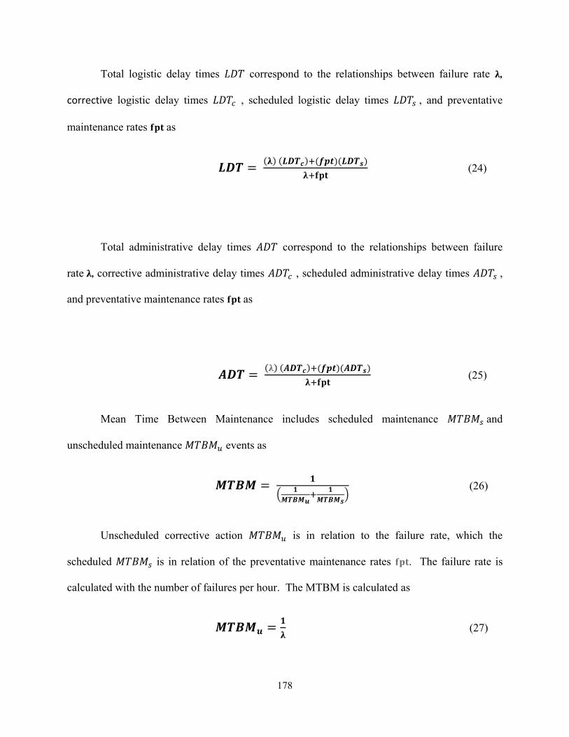
178

Total logistic delay times 𝐿𝐷𝑇 correspond to the relationships between failure rate 𝛌,

corrective logistic delay times 𝐿𝐷𝑇𝑐 , scheduled logistic delay times 𝐿𝐷𝑇𝑠 , and preventative

maintenance rates 𝐟𝐩𝐭 as

𝑳𝑫𝑻 = (𝛌) (𝑳𝑫𝑻𝒄)+(𝒇𝒑𝒕)(𝑳𝑫𝑻𝒔)𝛌+𝐟𝐩𝐭 (24)

Total administrative delay times 𝐴𝐷𝑇 correspond to the relationships between failure

rate 𝛌, corrective administrative delay times 𝐴𝐷𝑇𝑐 , scheduled administrative delay times 𝐴𝐷𝑇𝑠 , and preventative maintenance rates 𝐟𝐩𝐭 as

𝑨𝑫𝑻 = (𝛌) (𝑨𝑫𝑻𝒄)+(𝒇𝒑𝒕)(𝑨𝑫𝑻𝒔)𝛌+𝐟𝐩𝐭 (25)

Mean Time Between Maintenance includes scheduled maintenance 𝑀𝑇𝐵𝑀𝑠 and

unscheduled maintenance 𝑀𝑇𝐵𝑀𝑢 events as

𝑴𝑻𝑩𝑴 = 𝟏( 𝟏𝑴𝑻𝑩𝑴𝒖+ 𝟏𝑴𝑻𝑩𝑴𝒔) (26)

Unscheduled corrective action 𝑀𝑇𝐵𝑀𝑢 is in relation to the failure rate, which the

scheduled 𝑀𝑇𝐵𝑀𝑠 is in relation of the preventative maintenance rates 𝐟𝐩𝐭. The failure rate is

calculated with the number of failures per hour. The MTBM is calculated as

𝑴𝑻𝑩𝑴𝒖 = 𝟏𝛌 (27)

179

𝑴𝑻𝑩𝑴𝒔 = 𝟏𝐟𝐩𝐭 (28)

𝑴𝑻𝑩𝑴 = 𝟏(𝛌+𝐟𝐩𝐭) (29)

Operational Availability 𝐴𝑜 is calculated by the relationship between MTBM and MDT as

𝑨𝒐 = 𝑴𝑻𝑩𝑴(𝑴𝑻𝑩𝑴+𝑴𝑫𝑻) (30)

Designing and planning for reliability prevents failures. Reliability is the probability of an

item to perform a required function under stated conditions for a specified period of time,

availability is a measure of the degree to which an item is in an operable state and can be committed

at the start of a mission when the mission is called for at an unknown (random) point in time, and

maintainability is the ability of an item to be retained in, or restored to, a specified condition when

maintenance is performed by personnel having specified skill levels, using prescribed procedures

and resources, at each prescribed level of maintenance and repair [109]. Availability is the

amount of time a system is in operational condition. Availability is the ratio of the system’s uptime

to downtime. Maintainability involves the ease of a system being maintained to operational status.

The time it takes to repair an item and to perform preventive / corrective maintenance procedures

are included within the maintainability criteria. RAM of a system are critical for overall

operational availability. Operational availability of a system is essential for continuous operations

without interruption.

5.2 Testing Process Analysis

Testing antenna systems prior to fielding identifies any potential issues and verifies

equipment operation. Although manufacturers may test systems to a certain extent, integration

180

testing may be limited due to interconnecting system availability that the manufacturer has access

to. Antenna systems would go through a Pre-Installation Test and Check Off (PITCO) procedure

prior to fielding the system. Performing a PITCO would ensure the system is operational prior to

fielding within a live environment. Identifying issues prior to fielding reduces the chances of

encountering problems once the antenna system is installed.

An Integration Definition for Process Modelling (IDEF0) is used to depict the testing

process as shown in Figure 78. A scenario where antenna equipment is received from the

manufacturer that requires PITCO prior to fielding is depicted within an IDEF0. Untested

equipment would be received and stored in the warehouse until requested to be tested. Once the

system is scheduled to be tested, the equipment is transported to the integration area where

additional parts and pieces are added onto the system to simulate the environment on which it’s

fielded. The untested equipment is delivered to the lab to perform PITCO on the system. If failed

parts are identified during PITCO, a request to cannibalize parts is made if spare parts are not

available. Cannibalizing parts involve taking parts off of existing antenna systems received from

the manufacturer to prevent logistical delays relating to spare part procurement. Once the antenna

equipment is tested, the equipment is sent back to the integration area where the additional parts

and pieces are removed from the system. The antenna system is sent back to the main warehouse

to be prepped for shipping to the fielding site. Figure 78 PITCO Testing IDEF0 depicts the process

of equipment being integrated and tested by key logistic, engineering, and SME personnel.

181

Figure 78 PITCO Testing IDEF0

SE simulation tools are useful to predict overall process times to ensure delivery schedules

are met for fielding. Issues can also be identified such as bottlenecks in certain areas of the process

where management intervention would take place to take corrective actions. ExtendSIM was used

to simulate PITCO processing times. Known process areas, historical data and estimates were

used to evaluate probable processing times in particular areas. The triangular distribution was

used at various instances to list values for the minimum, most likely, and the maximum amount of

time. These values would be picked randomly over numerous iterations to provide an average

value to perform PITCO. The simulation involved three areas to include the main warehouse,

integration staging area, and the PITCO lab. These areas had a variable amount of time where the

182

antenna system would reside throughout the PITCO process. Inquiries on how long the process

would take was fulfilled by simulation. Providing an estimated time to perform the task allowed

for improved scheduling of fielding the antenna systems.

The untested equipment would be received at the main warehouse where an associated

logistics delay time using the triangular distribution of 1 day being the minimum, 3 days being the

maximum and 2 days being the most likely values that the untested antenna system would be at

that location. The process continues where the untested antenna system would get integrated with

various components in the integration staging area. Integrating the antenna system with

components were needed to simulate the system within a life like environment. The triangular

distribution for this part of the process would be 1 day for the minimum, 3 days being the

maximum, and 2 days being the most likely values. The PITCO lab would receive the untested

integrated antenna system to perform testing. PITCO times vary from 5 days being the minimum,

14 days being the maximum, and 8 days being the most likely values. There are instances where

issues are encountered. The request for replacement parts or the request for cannibalizing an

existing system is called for once the issue is isolated to a particular part or component. Historical

data has found that a replacement part or component was required 10% of the time. Providing a

part or cannibalizing an existing system typically takes 0.1 days at minimum, 0.3 days maximum,

with 0.2 days being the most likely value. If there are no issues encountered during testing, the

tested antenna system is sent back to the integration staging area where the components and parts

added previously are removed. The minimum amount of time to process the equipment back to

the main warehouse is 1 day. The maximum amount of time is 15 days where the most likely time

is 5 days. A potential bottleneck is present here with the maximum amount of time being in this

area constitutes to being 15 days. The main warehouse obtains the tested antenna system and has

183

a minimum value of 1 day, maximum value of 5 days, and a most likely value of 3 days. The

antenna system is prepped for shipping and sent to its fielded destination. Figure 79 Simulated

PITCO Process depicts the ExtendSIM model to predict PITCO processing times.

Figure 79 Simulated PITCO Process

Using the probability density function for triangular distribution allows minimum,

maximum, and most likely values to be entered. These values can be used repeatedly during

multiple iterations of the simulation. The probability density function of the triangular distribution

is:

184

𝒇(𝒙|𝒂, 𝒃, 𝒄) = { 𝟐(𝒙−𝒂)(𝒃−𝒂)(𝒄−𝒂) ; 𝒂 ≤ 𝒙 ≤ 𝒄𝟐(𝒃−𝒙)(𝒃−𝒂)(𝒃−𝒄) ; 𝒄 ≤ 𝒙 ≤ 𝒃 𝟎 ; 𝒙 < 𝒂, 𝒙 > 𝒃 (31)

The triangular distribution provides upper and lower limitations on values decreasing the

chances for any extreme values. The minimum value is denoted as a, the maximum value is

denoted as b, and the most likely value is denoted as c. Figure 80 depicts the triangular distribution

using these values.

Figure 80 Probability Density Function for Triangular Distribution

This distribution starts at 0 with the minimum value of a, rises to the most likely value of

c, then returns to 0 with the maximum value of b. This distribution provides a linear depiction of

the minimum, maximum, and most likely values. The triangular distribution probability value at

peak c is:

𝟐(𝒃−𝒂) (32)

The average PITCO process was estimated at 25 days. ExtendSIM was able to simulate

the process using triangular distributions at each process area. The PITCO lab had the SATCOM

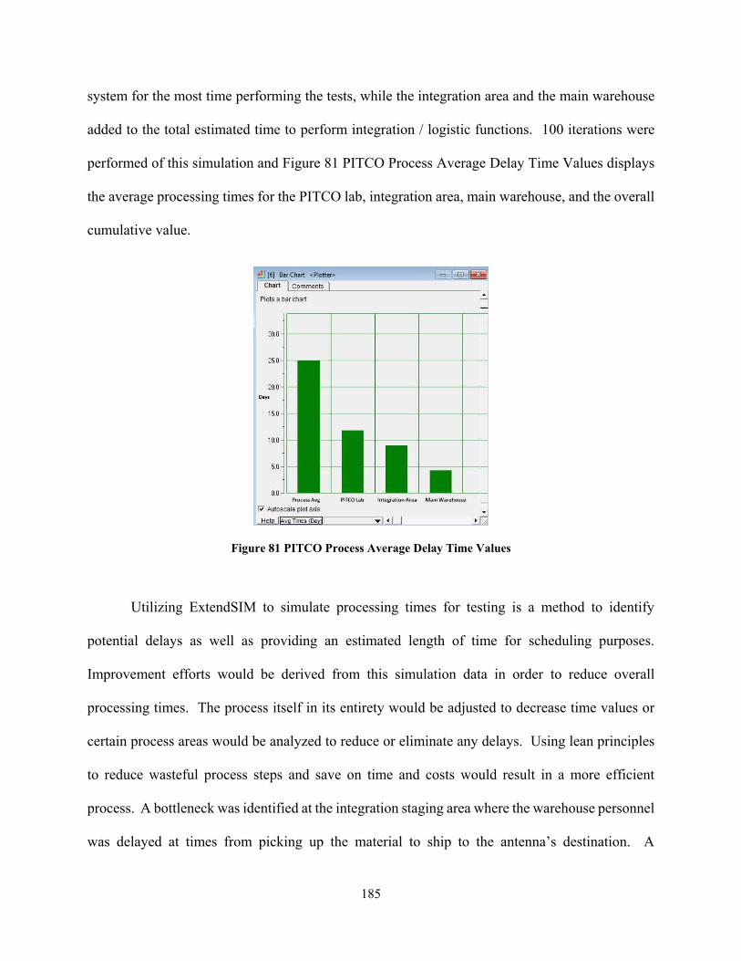
185

system for the most time performing the tests, while the integration area and the main warehouse

added to the total estimated time to perform integration / logistic functions. 100 iterations were

performed of this simulation and Figure 81 PITCO Process Average Delay Time Values displays

the average processing times for the PITCO lab, integration area, main warehouse, and the overall

cumulative value.

Figure 81 PITCO Process Average Delay Time Values

Utilizing ExtendSIM to simulate processing times for testing is a method to identify

potential delays as well as providing an estimated length of time for scheduling purposes.

Improvement efforts would be derived from this simulation data in order to reduce overall

processing times. The process itself in its entirety would be adjusted to decrease time values or

certain process areas would be analyzed to reduce or eliminate any delays. Using lean principles

to reduce wasteful process steps and save on time and costs would result in a more efficient

process. A bottleneck was identified at the integration staging area where the warehouse personnel

was delayed at times from picking up the material to ship to the antenna’s destination. A

186

recommendation would include shipping and receiving directly from the integration staging area

instead of shipping to the main warehouse. The main warehouse was a central point where the

entire organization would ship and receive material. An exception to the organizational process

via the organization process owner would be presented for a process improvement initiative

depicting the amount of time and costs saved. In addition, having a spares repository in the PITCO

lab would allow testers to quickly replace a part instead of manually retrieving the part from the

remote integration staging area where the spares are kept. Figure 82 depicts the simulated PITCO

process after lean improvements.

Figure 82 Simulated Lean PITCO Process

Upon performing lean practices on the known process, delay times can be reduced. The

integration staging area would perform functions such as receiving, shipping, integration and other

logistics services while the PITCO lab would perform PITCO as well as providing replacement

187

parts as required. The minimum amount of days to receive, provide logistics support and

integration in the integration staging area would be 1 day while the maximum amount of days

would be 5 days. The most likely amount of days to perform these functions would be 3 days.

The PITCO lab would perform PITCO and provide replacement parts with an estimated minimum

value of 5 days, maximum value of 14 days, and most likely be able to complete these tasks within

8 days. Once testing is complete, the integration staging area would prepare and ship the antennas

with a minimum value of 1 day, maximum value of 3 days, and most likely be able to complete

the task within 2 days. 100 iterations of the simulation were performed and the results are shown

in Figure 83 Lean PITCO Process Average Delay Time Values.

Figure 83 Lean PITCO Process Average Delay Time Values

Performing lean methodologies to known process areas can provide opportunities to reduce

cycle times. The known PITCO process can be reduced from 25 days to 11 days by making a few

adjustments to the process. These adjustments not only can reduce delay times for tasks but save

on overall costs. These adjustments can be used as lessons learned for any upcoming projects or

efforts that are similar in nature.

188

5.3 Production, Deployment, Operations and Support

The Production and Deployment phase consists of executing the LRIP as well as

determining the readiness for FRP&D. Evaluations of the first line of systems would be performed

to potentially improve the production process, quality of system and any other processes that

reduces cost / schedule. The Production and Deployment phase begins after Milestone C. The

product baseline is updated in this phase where any changes made on the system to correct issues

or to enhance particular aspects of the system to support improved producibility, fielding, usability,

and any other changes that are required. The test and evaluation plan would also be updated to

include any testing related to the production and deployment phase. These tests would include

PITCO and SOVT documents. PITCO would entail performing tests prior to the system being

fielded. Performing PITCO would identify any issues with the system prior to the system being

fielded. If this test was not performed, there would be a risk that a fielded system would have

issues. The amount of rework to re-install a working system would me more than performing a

PITCO prior to install. A SOVT would entail performing tests once the system is fielded which

verifies operational functions the system would perform. Risk management would continue to be

performed to identify any cost, schedule and technical risks that may be associated with production

and deployment efforts. The life cycle sustainment plan would be updated to include new

information on sustaining the system. Logistics support functions such as storage, personnel and

other resources that have been uncovered or became more detailed would be documented within

the life cycle sustainment plan. Any new or detailed maintenance support needs would also be

documented within the life cycle sustainment plan or be referenced for access. The Systems

Engineering Plan would be updated to include up to date production and deployment efforts and

operation support functions. Standard operating procedure documents would be referenced to

189

support the system to assist with maintenance and sustainment needs of the system. Ensuring any

safety, environmental and health compliance documents are up to date is another activity within

the production and deployment phase. The Full Rate Production Decision Review occurs to concur

amongst stakeholders to go forward with manufacturing the large scale of parabolic stacked

antenna systems. Assessing the LRIP of the systems with regards to lessons learned,

manufacturing processes, potential defects, additional needed resources and an overview of

production cost, schedule, and performance factors gives stakeholders confidence that full rate

production of the parabolic antenna system can begin.

Operations and support has the system installed and is verified during the SOVT. Once

the SOVT is completed, the system is handed over to the warfighter to maintain. Standard

operating procedures along with training allows the warfighter to operate the system effectively.

Training personnel initially as well as recurring training equips personnel with being able to

operate, maintain, and troubleshoot the system without the need for external support. External

support includes system help desk support for offsite and possible onsite support. Obtaining

metrics for help desk trouble tickets provides insight on high failure items, defects, system issues

or possible issues with training or operating procedures. Upgrades and modifications are included

within this phase to enhance or fix any issue or any potential vulnerability. Software updates

provide software bug fixes and information assurance vulnerability mitigations. Depending on the

complexity of the modification to the system, the modification may or may not include assistance

from SMEs. A low cost option for a not so complex modification entails providing the

modification material / software to the user to perform themselves.

The system maintenance concept should include the entire system and not just a particular

part of the system. Other areas are to consider are maintenance to other systems interoperating

190

with the system. The system maintenance concept should be developed during the conceptual

design phase which evolves from the definition of system operational requirements. Support

concepts include:

Levels of Maintenance: This could include a basic level of maintenance where the actual

user can perform themselves (i.e. inspect and perform weatherproofing procedures on connections

to the antenna) as opposed to a professional performing more advanced maintenance activities (i.e.

azimuth and elevation motor replacement).

Repair Policies: This would include establishing a baseline or agreement during the

conceptual design process, which includes a repair strategy or policy that the customer / operator

can adhere to (i.e. grease azimuth and elevation motors every 3 years).

Organizational Responsibilities: Responsibilities would be agreed upon via the repair

policies where a user’s responsibilities would need to be kept in order for them to maintain product

warranty (i.e. Documentation of maintenance performed within 10 years need to be kept in order

to provide antenna support during that time frame). Organizational Responsibilities may differ

from the customer than the manufacturer of the system or component.

Maintenance support elements: Spares, man-power, etc. would be a part of maintenance

support elements.

Effectiveness Requirements: This would include the availability of these items and the

associated criteria for these resources. Factors will include the support capability associated with

personnel, spares, demand rate, reliability, etc.

191

Environment: This would include shock, vibration, temperature and any other

environmental factors that may have an effect on the system.

A system engineering model used to depict functional analysis is a Functional Flow Block

Diagram (FFBD). A FFBD illustrates high level and lower level functions with traceability. The

consolidated antenna development would include identifying the need, determining the

requirements, design, testing, manufacturing, deploying, and operating / sustaining the system.

The FFBD model is shown in Figure 84 to illustrate operation and maintenance activities involved

in the consolidated antenna system’s life cycle.

Figure 84 FFBD WRT System Operation and Maintenance

The FFBD example shows lower level activities associated with operating and maintaining

a consolidated antenna system such as the parabolic stacked antenna. Basic operation functions

are decomposed to lower level functions that link to maintenance actions. For this case a system

192

log files reveals the need to remove / replace scheduled maintenance components. This high level

FFBD assists with functional analysis of the overall system being developed.

Reliability deals with probability and statistical approach required when deriving reliability

factors. Reliability is dependent on the design details. Input from SMEs are included to select

particular components or sub systems. System designers, testers, manufacturers, installation team,

product support team, users, maintainers, and other SMEs would be consulted to obtain RAM

requirements. Maintainability requirements would be considered early on to address components

to replace. Considering easy access for users is essential for repair or maintenance procedures.

Repairing a parabolic stacked antenna would have to consider onsite repair procedures. A radome

that houses a parabolic stacked antenna would limit the amount of space a user can use when

repairing / maintaining the consolidated antenna. As shown in Figure 85, limited space to

physically repair / maintain the antenna is observed.

Figure 85 NMT Antenna in Radome Space [69]

Usability factors have to be addressed, such as performing repair / maintenance procedures.

To perform repairs for the NMT antenna shown in Figure 85 for example, the antenna would have

to be in a position where the user would be able to access certain components. Certain height and

weight restrictions would be denoted for safety criteria in regards to being inside the radome with

the antenna in place. Considerations for a user to get into and out of the radome to access the

antenna is necessary in order to provide a cost effective repair / maintenance procedure.

193

Identifying critical items whose reliable operation is critical to the operation of the system. A

critical item list would be identified for components and subsystems. Issues can be mitigated

through the design process through design changes early within the system’s life cycle. Identifying

a single point of failures is essential to provide potential redundancy options. Reliability

requirements defined early and determining if they are achievable is performed in the requirements

definition phase. During functional analysis and allocation having a tradeoff study with an AoA

can affect a choice by different reliability criteria. Design synthesis includes reviewing system

and subsystem design, and maximizing redundancy with respect to tradeoffs with reliability,

operational performance and system cost. Performing a Failure Mode, Effects & Criticality

Analysis assists engineers to understand the system’s failure modes with critical / single point of

failures. Critical components would be monitored regularly to be inspected, repaired or replaced.

Using de-rating factors such as the environment would account for the effects. The amount of

time to put forth effort on performing RAM activities throughout the system’s life cycle should be

considered. Increasing design with more reliability details would increase schedule, but will

prevent issues from surfacing later in the system’s life cycle. Characterizing reliability criteria

along with potential testing and data mining for historical data would increase the schedule as well,

but have benefits in the long term. Adding additional components for redundancy may involve

increasing the space and weight that the overall system encompasses.

The initial cost of a reliable system would cost more to develop, but would benefit during

the sustainment phase of the system lifecycle by increasing the longevity of the system. Less

reliable systems and components cost less initially but require more maintenance during the

sustainment phase of the system’s life cycle. Including reliability, availability, and maintainability

194

criteria during the early phases of design would reduce overall life cycle costs by reducing rework,

maintenance and sparing during the later stages of the system’s life cycle.

195

6. Summary

Developing a consolidated antenna with multiband frequency capabilities can be achieved

by performing SE activities and leveraging lessons learned from previous antenna consolidation

efforts. Using parabolic antenna stacking methods consolidates multiple antenna capabilities onto

a single pedestal. The NMT, CBSP and directional SDT antennas were assessed to determine RF

capability requirements to design a single pedestal antenna to meet RF capabilities that the

SATCOM and LoS antennas currently operate within. Prior consolidation efforts such as the NMT

system was analyzed to determine life cycle costs throughout the DAS process. Cost estimates

were determined by previous and projected budgets that were used for the NMT system to predict

potential cost needs for developing a parabolic stacked antenna system. Agile and lean

methodologies were proposed to reduce costs and delivery time frames. Use case scenarios were

depicted to illustrate various operations that the parabolic stacked antenna would be capable of.

Simulating processes demonstrates delay times especially with repeatable processes. Process

simulation would identify potential improvement areas and predict delay times within each step of

the process. A testing process was simulated to propose estimated delay times utilizing a triangular

distribution probability set. The triangular distribution probability set included best, worst, and

most likely time values based on historical process times at each step of the process. Lean

methodologies were introduced to improve known process areas by reducing unneeded steps.

Following the DAS process provided an approach to develop a parabolic stacked antenna.

Cassegrain, Gregorian and splash plate antennas were analyzed using the parabolic stacking

method to determine the physical parameters and RF capabilities associated with each. A

combination of the splash plate, Gregorian and Cassegrain antennas were also analyzed. The

results showed that splash plate antennas using the parabolic stacking method required only two

196

antennas to achieve RF capabilities that current NMT, CBSP and directional SDT antennas

provide. The large X / Ka NMT and CBSP FLV variants have a parabolic dish diameter of 2.44m

and 2.74m respectively. These two antennas provide limited RF coverage such as X, Ka bands for

the large X / Ka NMT antenna and L, C, and Ku bands for the CBSP FLV variant. The parabolic

stacked antenna using splash plate antennas is not only smaller (2.25m) than the large X / Ka NMT

and CBSP FLV variants but also includes RF coverage that the other NMT and CBSP variants

provide along with the directional RF capability of the SDT antenna. The dual splash plate

parabolic stacked antenna is capable of operating at frequencies within the L, C, Ku, K, Ka, X and

Q bands. The triple Cassegrain parabolic stacked antenna and dual cassegrain with splash plate

parabolic stacked antenna proved that three antennas can be stacked in front of one another to meet

operational requirements. Parabolic antenna stacking is possible when the reflecting dish produces

a blockage area that another antenna could utilize to operate within to gain additional RF bands.

The Gregorian with splash plate parabolic stacked antenna had a maximum dish size of 1.5m and

was capable of operating within C, Ku, K, Ka, X and Q band frequency ranges. The Cassegrain

and Gregorian parabolic stacked antenna had the same main dish size of 1.5m for the larger antenna

as well as the main dish size of 325.9mm for the smaller antenna compared to the Gregorian and

splash plate parabolic stacked antenna configuration. The Cassegrain and Gregorian parabolic

stacked antenna had a higher VSWR value for select frequencies when compared to the Gregorian

with splash plate parabolic stacked antenna. The dual Gregorian parabolic stacked antenna was

larger and had a maximum dish size of 1.921m. The dual Gregorian parabolic stacked antenna

was capable of the same frequency set and had slightly higher gain values. The triple Cassegrain

parabolic stacked antenna and the dual splash plate parabolic stacked antenna were capable of

197

operating at a particular sized antenna along with the next sized antenna stacked in front of it. This

capability provides redundancy with potential failover options for overall operational availability.

Utilizing SE practices support decision making challenges that are encountered throughout

the system life cycle. The Pugh matrix is recommended to be used with stakeholders to determine

which design concept for the parabolic stacked antenna would be the best option to go forward

with. Considering the design criteria, the parabolic stacked antenna option using dual splash plate

antennas on a single pedestal was the best option to achieve L, C, X, Ku, K, Ka and Q band

frequencies. A decision matrix could also be used for other areas where various options are present

that need to be compared amongst different alternatives. This methodology provides a brief

analysis of alternatives to facilitate decisions from stakeholders.

Developing a baseline schedule assists with future planning and manage stakeholder

expectations. Considering the previous NMT system going through the DAS process, a similar

timeline is followed for developing the parabolic stacked antenna to perform SE, MBSE, Agile

and lean activities throughout the process. The Materiel Solution Analysis phase would last

approximately 2 years, and the Technology Maturation and Risk Reduction phase would span

across 2 years as well. The Engineering and Manufacturing development phase would span over

5 years using the DAS process incorporating Agile methodologies. The Production and

Deployment phase would last for approximately 8 years where performing lean methodologies to

known process areas while reducing planned procurement actions required for additional spares /

antenna upgrades by procuring them in advance would assist with meeting this timeline. The

Operations and Sustainment phase is planned to last 22 years which is similar to the Operations

and Sustainment phase of the NMT system in which the service life of the parabolic antenna system

is baselined against. The approximate life cycle costs for the NMT system was estimated to be

198

$2,646.4M. Reducing schedule for the Engineering & Manufacturing Development phase and the

Production and Development phase by 3 years each would have a cost savings of $419.2M.

Reducing these times would depict a baseline budget of $2,227.2M over 32 years for the parabolic

stacked antenna system life cycle. Combining SDT, NMT, CBSP antenna platforms would reduce

overall life cycle costs maintaining multiple systems. Additional cost savings would be realized

from the Operations and Support phase for maintaining one antenna system as opposed to two.

The approximate life cycle costs for the parabolic stacked antenna system was $2,227.2M over 32

years. Considering life cycle costs for two systems would amount to approximately $4,454.4M

over 32 years. A life cycle cost savings of ~$2B over 32 years would be potentially realized by

developing one consolidated system vice two individual systems.

Processing times is important to predict and incorporate delay times into schedule and to

estimate the availability of the system. Simulating processing times identifies potential bottlenecks

within the process that could be improved upon using lean methodologies. Using historical data

for processing times and simulating processes using triangular distribution probability density

functions creates estimated delay times to factor into schedule and system availability. A test

process was simulated to determine delay times within each step of the process. These values can

be used to determine the operational availability of a system when testing a replacement antenna

is required. Testing the system produces delay times which would prompt the need to have spare

systems and parts available if needed while considering the failure rate of the system itself.

Capturing metrics on processing times along with metrics on help desk tickets during the

Operations and Support phase of the life cycle will improve and maintain overall operational

availability of the system.

199

This dissertation provided a consolidation approach using MBSE SysML models to

identify interconnecting RF system criteria which revealed overlap of RF capabilities. This finding

further stresses the longstanding need to reduce the amount of redundant antenna systems.

Parabolic stacked antenna simulations of six different configurations identified tradeoffs amongst

Cassegrain, Gregorian and splash plate antennas. Cost savings were realized by applying lean

methodologies for practical efforts such as the PITCO process through simulating, assessing and

improving PITCO process steps. Performing SE, MBSE, Agile and lean methodologies can assist

with today’s complex integrated systems. As technology advances, so does the complexity of

systems. SE and MBSE modeling can help manage these complex systems by depicting

interactions between integrated systems and also identify potential areas of concern through

simulation. MBSE efforts should be used along with SE standard processes and Agile / lean

methodologies to be able to achieve the most cost effective and timely solution.

6.1 Future Work

This research focuses on system engineering of a parabolic stacked antenna to minimize

space taken from multiple antenna platforms performing similar functions, decrease overall life

cycle costs and decrease time to develop this new capability. Combining multiple antennas upon

a single pedestal using the parabolic stacked antenna methodology allows multiple RF bands to be

accessed by a single antenna based platform. Performing simulation testing provides evidence that

multiple RF bands on a single pedestal can be achieved. There are limitations for the parabolic

stacked antenna simulation results where deviations would be realized when testing a prototype

within an anechoic chamber. The prototype would have to be fabricated with particular materials

that have slight variations with the material specifications. These slight variations provide a

tolerance for RF fabricated components where simulations presented within this dissertation are

200

set to a fixed value within the CST Microwave simulation software. Precision with fabricating the

parabolic stacked antenna prototype would be needed to decrease measurement errors when

comparing the simulation results to the physical prototype testing results. Avenues for continuing

research of the system engineering of a parabolic stacked antenna include:

Simulation of different types of parabolic stacked antenna configurations to provide

alternatives to consolidate the NMT, CBSP, SDT and other variant antennas

Continuing to capture simulation data to assess antenna problem areas with regards to

frequency, VSWR, gain, side lobe levels, angular width (3 dB), interference and blockage

Reducing design / development times and cost to produce a parabolic stacked antenna by

detailing SE / Agile methodologies and possible alternative approaches

Prototyping a physical parabolic stacked antenna to compare against simulation results

Developing and determining the location of consolidated RF amplifiers and feeds to account

for L, C, X, Ku, K, Ka and Q band frequencies

Identifying additional risk areas and mitigating known risks for the design and development

of a parabolic stacked antenna

201

References

[1] "5 WORKERS HURLED TO DEATHS AS A TEXAS TOWER COLLAPSES," NY Times, 8

December 1982. [Online]. Available: https://www.nytimes.com/1982/12/08/us/5-workers-hurled-

to-deaths-as-a-texas-tower-collapses.html. [Accessed 30 January 2019].

[2] "Engineering Ethics TV Antenna Collapse," Texas A&M Department of Philosophy and

Department of Mechanical Engineering, June 1992. [Online]. Available: http://ethics.tamu.edu/wp-

content/uploads/sites/7/2017/04/TVAntennaCollapse.pdf. [Accessed 30 January 2019].

[3] "Galileo Antenna Deployment Problem Under Analysis," NASA Jet Propulsion Labrotory, 19 April

1991. [Online]. Available: https://www.jpl.nasa.gov/news/news.php?feature=5661. [Accessed 1

February 2019].

[4] M. A. Stein, "Effort to Fix Space Probe's Antenna Fails : NASA: Device on Jupiter-bound craft

remains jammed. Failure to deploy it will severely reduce the number of photos that can be relayed

to Earth in 1995," Los Angeles Times, 31 December 1992. [Online]. Available:

http://articles.latimes.com/1992-12-31/local/me-4278_1_high-gain-antenna. [Accessed 1 February

2019].

[5] P. ". Jansma, "Open! Open! Open! Galileo High Gain Antenna Anomaly Workarounds," 2011

Aerospace Conference, p. 21, 5-12 March 2011.

[6] IBM, 2019. [Online]. Available:

https://www.ibm.com/support/knowledgecenter/en/SSYQBZ_9.6.1/com.ibm.doors.requirements.d

oc/topics/c_welcome.html. [Accessed 25 Jan 2019].

[7] "What can IBM Rational Rhapsody products do for you?," IBM, 2019. [Online]. Available:

https://www.ibm.com/us-en/marketplace/rational-rhapsody. [Accessed 25 January 2019].

[8] "Innoslate," SPEC Innovations, 2017. [Online]. Available: https://www.innoslate.com/. [Accessed

15 November 2018].

[9] "ExtendSim™ - Simulation Modeling Software," Extended Answers, 2008. [Online]. Available:

www.extendedanswers.com/extendsim.html. [Accessed 15 November 2018].

[10] "Antenna Magus," CST Computer Simulation Technology GmbH, 2018. [Online]. Available:

https://www.cst.com/products/antennamagus. [Accessed 15 September 2018].

[11] F. Pellerano, "Systems Engineering," in Thermal & Fluids Analysis Workshop, Greenbelt, 2015.

202

[12] "Request for Information N00014-16-R-RFI4 Electromagnetic Maneuver Warfare Command &

Control (EMC2) Low-band Radio Frequency Intelligent Distribution Resource (LowRIDR),"

Department of Defense, San Diego, 2016.

[13] D. Putnam, "(SBIR) Navy - Consolidated Apertures with Co-site Interference Reduction in the

Frequency Range 2 to 30 MHz," 2010. [Online]. Available: http://www.navysbir.com/n10_2/N102-

159.htm. [Accessed 31 August 2017].

[14] "CVN-73," Navy.com, 2017. [Online]. Available: https://www.navy.com/dam/Navy/Navy-

IMG/About-IMG/equipment/vessels/carriers/130823-N-IY633-124_CRP-1-2/130823-N-IY633-

124_CRP-1-1.jpg. [Accessed 31 August 2017].

[15] "Raytheon to Provide Navy Multiband Terminals," SIGNAL Magazine, 2015. [Online]. [Accessed

6 September 2017].

[16] "Commercial Broadband Satellite Program (CBSP) | Harris," Harris.com, 2017. [Online]. Available:

https://www.harris.com/solution/commercial-broadband-satellite-program-cbsp. [Accessed 06

September 2017].

[17] J. Keller, "Navy makes $10.3 million order to Harris to provide SATCOM aboard big surface

warships," 26 February 2016. [Online]. Available:

https://www.militaryaerospace.com/articles/2016/02/satcom-surface-warships.html. [Accessed 6

September 2017].

[18] "SHARK LINK SURFACE DATA TERMINAL (SDT)," Cubic Mission Solution, 2017. [Online].

Available: https://www.cubic.com/sites/default/files/6883_1000141-Sharklink_SDT_NCM_0.pdf.

[19] C. Sugama, "Organizational Communication System Cybersecurity," International Journal of

Engineering Research & Technology, vol. 6, no. 7, pp. 192-195, 2017.

[20] C. Sugama, "Engineering of a Dynamic Multi-Frequency Antenna," International Journal of

Engineering Research & Technology, vol. 6, no. 7, p. 19, September 2018.

[21] "USN Ship Protection: From “Slick 32s” to SEWIP," February 2019. [Online]. Available: https://www.defenseindustrydaily.com/us-navy-from-slick-32s-to-sewip-05365/.

[22] "Integrated Topside," Office of Naval Research, [Online]. Available:

https://www.onr.navy.mil/en/About-ONR/History/tales-of-discovery/integrated-topside.

[23] S. a. N. W. S. C. P. Affairs, "Navy's New Broadband Satellite Program Provides Greater

Reliability," U.S Navy, December 2008. [Online]. Available:

https://www.doncio.navy.mil/chips/ArticleDetails.aspx?ID=2741.

203

[24] J. Hughes, "CHIPS Articles: It's Time to Change the Way We Refer to SHF Satellite

Communications," Doncio.navy.mil, 2012. [Online]. Available:

http://www.doncio.navy.mil/chips/ArticleDetails.aspx?ID=4213. [Accessed 22 August 207].

[25] "Satellite frequency bands," European Space Agency, 2013. [Online]. Available:

http://www.esa.int/Our_Activities/Telecommunications_Integrated_Applications/Satellite_frequen

cy_bands. [Accessed 24 August 2017].

[26] P. Anuszkiewicz , A. Allison , D. Bethea-Murphy , M. Brown, M. Calabrese and T. Dombrowsky,

"Identifying Key Characteristics of Bands for Commercial Deployments and Applications

Subcommittee Final Report and Recommendations," 17 November 2017. [Online]. Available:

https://www.ntia.doc.gov/files/ntia/publications/key_characteristics_sub-

committee_final_report_nov_17_2017.pdf. [Accessed 28 June 2019].

[27] "Wideband Global SATCOM (WGS) Satellite," Aerospace Technology, 2017. [Online]. Available:

http://www.aerospace-technology.com/projects/wgs-satellite. [Accessed 16 August 2017].

[28] "Defense Satellite Communications System," Af.mil, 2015. [Online]. Available:

http://www.af.mil/About-Us/Fact-Sheets/Display/Article/104555/defense-satellite-

communications-system/. . [Accessed 16 August 2017].

[29] "Advanced Extremely High Frequency System," Afspc.af.mil, 2017. [Online]. Available:

http://www.afspc.af.mil/About-Us/Fact-Sheets/Display/Article/249024/advanced-extremely-high-

frequency-system. [Accessed 16 August 2017].

[30] "Milstar Satellite Communications System," Afspc.af.mil, 2017. [Online]. Available:

http://www.afspc.af.mil/About-Us/Fact-Sheets/Display/Article/1012622/milstar-satellite-

communications-system/.. [Accessed 18 August 2017].

[31] "Milstar Satellite Communications System," Afspc.af.mil, 2017. [Online]. Available:

http://www.afspc.af.mil/About-Us/Fact-Sheets/Display/Article/1012622/milstar-satellite-

communications-system. [Accessed 18 August 2017].

[32] "Intelsat 29e, the First Intelsat Epic^NG Satellite, Successfully Launched into Orbit |

Intelsat," Intelsat, 2016. [Online]. Available: http://www.intelsat.com/news/press-release/intelsat-

29e-the-first-intelsat-epicng-satellite-successfully-launched-into-orbit/. . [Accessed 23 August

2017].

[33] S. D. McNeil, "INMARSAT-3 F3 (178.1° E.L.)," [Online]. Available:

https://licensing.fcc.gov/myibfs/download.do?attachment_key=-136047. [Accessed August 15

2017].

[34] "Global Xpress - Inmarsat," Inmarsat, 2017. [Online]. Available:

https://www.inmarsat.com/service/global-xpress/. [Accessed 24 August 2017].

204

[35] "CBSP ULV," Harris Corporation, 2018. [Online]. Available:

https://www.harris.com/sites/default/files/downloads/solutions/d0883-cbsp-ulv-final.pdf.

[Accessed 20 September 2018].

[36] "CBSP FLV," Harris Corporation, 2018. [Online]. Available:

https://www.harris.com/sites/default/files/commercial_broadband_satellite_program_force_level_

variant.pdf. [Accessed 20 August 2018].

[37] Y.-C. Chang, B. Mui, J. Hanlin and A. Movva, "NMT X/Ka Tri-Band Antennas," in MILCOM 2012

- 2012 IEEE Military Communications Conference, Orlando, 2012.

[38] "NMT Navy Advanced Extremely High Frequency Multi-band Terminal," U.S. Navy, 2010.

[Online]. Available: http://www.secnav.navy.mil/rda/Pages/Programs/NMT.aspx. [Accessed 11

December 2018].

[39] A. Einhorn and J. Miller, "Spectrum Management Issues Related to the AEHF System," in MILCOM

2007 - IEEE Military Communications Conference, Orlando, 2007.

[40] L. J. J. Hughes, "DON CIO," DON, 7 December 2012. [Online]. Available:

http://www.doncio.navy.mil/mobile/ContentView.aspx?ID=4213&TypeID=21. [Accessed 7

December 2018].

[41] R. Williams and H. Paul, "Potential uses of the military Ka-band for wideband MILSATCOM

systems," IEEE Military Communications Conference. Proceedings. MILCOM 98 (Cat.

No.98CH36201), 19-21 Oct 1998.

[42] "Selected Acquisition Report (SAR) Global Broadcast Service (GBS) As of FY 2015 President's

Budget," September 2013. [Online]. Available: https://apps.dtic.mil/dtic/tr/fulltext/u2/a613515.pdf.

[Accessed 5 February 2019].

[43] "Light Airborne Multipurpose System (LAMPS) Hawklink," BAE Systems | United States, 2017.

[Online]. Available: http://www.baesystems.com/en-us/product/light-airborne-multipurpose-

system-lamps-hawklink.

[44] "Navy chooses AN/SRQ-4 ship-to-helicopter datalink radios from L3 for situational awareness,"

Military & Aerospace Electronics, 26 June 2013. [Online]. Available:

https://www.militaryaerospace.com/rf-analog/article/16715585/navy-chooses-ansrq4-

shiptohelicopter-datalink-radios-from-l3-for-situational-awareness.

[45] "CDL Hawklink AN/SRQ-4 Radio Terminal Set," L3 Communication Systems West, 2017.

[Online]. Available: https://www2.l3t.com/csw/assets/products/product-

sheets/CDL_Hawklink_AN-SRQ-4_Radio_Terminal_Set_Sales-Sheet_WEB.pdf.

205

[46] "Cooperative Engagement Capability (CEC) / AN/USG-2(V) Cooperative Engagement

Transmission Processing Set," Globalsecurity.org, 2017. [Online]. Available:

http://www.globalsecurity.org/military/systems/ship/systems/cec.htm.

[47] E. Ryen, "Overview of the System Engineering Process," March 2008. [Online]. Available:

https://www.dot.nd.gov/divisions/maintenance/docs/OverviewOfSEA.pdf. [Accessed 11 March

2018].

[48] "A Primer for Model-Based Systems Engineering," Vitech Corporation, Blacksburg, 2011.

[49] "U.S. Army | PEO C3T | Program Executive Office Command Control Communications-Tactical,"

Peoc3t.army.mil, 2017. [Online]. [Accessed 4 September 2017].

[50] "Global Broadcast Service," Afspc.af.mil, 2017. [Online]. Available:

http://www.afspc.af.mil/About-Us/Fact-Sheets/Article/249021/global-broadcast-service-gbs-joint-

program/. [Accessed 2017 August 29].

[51] "Aircraft carrier," Encyclopaedia Britannica, 2019. [Online]. Available:

https://cdn.britannica.com/34/94834-050-16DB7EEB/USS-Carl-Vinson-aircraft-carrier-US-Navy-

2005.jpg.

[52] A Guide to the Project Management Body of Knowledge, 6 ed., Chicago, IL: Project Management

Institute, 2017.

[53] D. F. Rico, "WHAT IS THE ROI OF AGILE VS. TRADITIONAL METHODS?," 2009. [Online].

Available: https://w.davidfrico.com/rico08b.pdf.

[54] D. F. Rico, "The Business Value of Using Agile Project Management for New Products and

Services," [Online]. Available: https://davidfrico.com/rico-apm-roi.pdf.

[55] "SAFe Case Study: PlayStation Network PlayStation Network Stays Top of its Game with SAFe,"

Scaled Agile, Inc, 2020. [Online]. Available: https://www.scaledagileframework.com/sony-

playstation-network-case-study/.

[56] "CASE STUDY: Fitbit Fitbit’s Agile Development Journey," Scaled Agile, Inc, 2020. [Online].

Available: https://www.scaledagileframework.com/fitbit-case-study/.

[57] D. Carney, S. Miller and M. A. Lapham, "Agile Development in Government: Myths, Monsters,

and Fables," Software Engineering Institute Carnegie Mellon University, September 2016. [Online].

Available: https://resources.sei.cmu.edu/asset_files/Brochure/2016_015_001_506324.pdf.

[58] "What's the Difference? Agile vs Scrum vs Waterfall vs Kanban," Smartsheet Inc, 2020. [Online].

Available: https://www.smartsheet.com/agile-vs-scrum-vs-waterfall-vs-kanban.

206

[59] P. Modigliani and S. Chang, "Defense Agile Acquistion Guide," MITRE Corporation, March 2014.

[Online]. Available: https://www.mitre.org/sites/default/files/publications/MITRE-Defense-Agile-

Acquisition-Guide.pdf.

[60] K. Beck, M. Beedle, A. v. Bennekum, A. Cockburn, W. Cunningham, M. Fowler, J. Grenning, J.

Highsmith, A. Hunt, R. Jeffries, J. Kern, B. Marick, R. C. Martin, S. Mellor, K. Schwaber, J.

Sutherland and D. Thomas, "Principles behind the Agile Manifesto," 2001. [Online]. Available:

http://agilemanifesto.org/.

[61] Agile Practice Guide, Newtown Square, Pennsylvania: Project Management Institute, Inc., 2017.

[62] D. J. Anderson and A. Carmichael, Essential Kanban Condensed, Seattle, WA: LeanKanban

University Press, 2016.

[63] M. Rehkopf, "Sprints," Atlassian, 2020. [Online]. Available:

https://www.atlassian.com/agile/scrum/sprints.

[64] "Scrum," Atlassian, 2020. [Online]. Available: https://www.atlassian.com/agile/scrum.

[65] "CASE STUDY: Fitbit Fitbit’s Agile Development Journey," Scaled Agile, Inc., 2020. [Online]. Available: https://www.scaledagileframework.com/fitbit-case-study/.

[66] "PI Planning," Scaled Agile, Inc., 2020. [Online]. Available:

https://www.scaledagileframework.com/pi-planning/.

[67] DoDI 5000.02 Operation of the Defense Acquisition System, 2015.

[68] "Model Based System Engineering," Scaled Agile, Inc., February 2020. [Online]. Available:

https://www.scaledagileframework.com/model-based-systems-engineering/.

[69] "Selected Acquisition Report (SAR) Navy Multiband Terminal (NMT)," 23 March 2016. [Online].

Available: https://apps.dtic.mil/dtic/tr/fulltext/u2/1019521.pdf. [Accessed 28 January 2019].

[70] R. Scharmann, "Harris Received $133 Million CBSP ULV Contract from US Navy," ViaSatellite,

25 April 2014. [Online]. Available: https://www.satellitetoday.com/government-

military/2014/04/25/harris-received-133-million-cbsp-ulv-contract-from-us-navy/.

[71] H. S. Kenyon, "Commercial Equipment Speeds Naval Communications, Replaces Aging

Hardware," AFCEA, February 2009. [Online]. Available:

https://www.afcea.org/content/commercial-equipment-speeds-naval-communications-replaces-

aging-hardware.

[72] ISO/IEC/IEEE 29148:2011 Systems and Software Engineering - Life Cycle Processes -

Requirements Engineering, 1 ed., New York: ISO/IEC/IEEE, 2011.

207

[73] "IBM Rational DOORS Next Generation," IBM, 2019. [Online]. Available:

https://jazz.net/products. [Accessed 23 January 2019].

[74] F. Sheldon, "Non-Functional Requirements," University of Colorado, 1999.

[75] "Getting started with Rational DOORS Next Generation," IBM, 2019. [Online]. Available:

https://www.ibm.com/support/knowledgecenter/SSYMRC_6.0.6/com.ibm.rational.rrm.help.doc/to

pics/c_compose_reqs.html. [Accessed 19 January 14].

[76] S. Burge, "The Systems Engineering Tool Box Pugh Matrix," p. 15, 2009.

[77] T. Smith, J. Granholm, O. S. Kim and O. Breinbjerg, "Combined L-band (1-2 GHz) and Ka-band

(20-30 GHz) Antenna". Patent Patent Application PCT/EP2013/050259, 2013.

[78] "The Cassegrain Antenna," Christian Wolff, [Online]. Available:

http://www.radartutorial.eu/06.antennas/Cassegrain%20Antenna.en.html.

[79] "Horn-fed Cassegrain reflector antenna," Magus, 2019. [Online]. Available:

http://www.antennamagus.com/database/antennas/antenna_page.php?id=97.

[80] P. Hazdra and M. Mazanek, "Reflector antennas and their feeds," elmag.org, Prague, 2015.

[81] "Horn fed Gregorian Axisymmetrical dual reflector," Magus (Pty) Ltd, 2019. [Online]. Available:

http://www.antennamagus.com/database/antennas/antenna_page.php?id=159.

[82] "Architecture of Gregorian Antenna," The MathWorks, Inc., 2020. [Online]. Available:

https://de.mathworks.com/help/antenna/ref/gregorian.html#mw_3ddf8fbd-7cae-4235-8f85-

d0f31a48c544.

[83] G. I. James and D. Malik, "Splash Plate Feed Design," 5th European Microwave Conference, pp.

41-45, 1975.

[84] E. CÜRÜK, C. ÖZDEMİR and K. YEĞİN, "A Novel Ultra-Wide Band Design for Feeding

Structure of Ka Band VSAT Parabolic Reflector Antenna," 21st International Conference on

Microwave, Radar and Wireless Communications (MIKON), 2016.

[85] "PTFE," Microwaves101.com, 2019. [Online]. Available:

https://www.microwaves101.com/encyclopedias/ptfe.

[86] G. J. Meyer, "Polyurethane Foam: Dielectric Materials for Use in Radomes and Other Applications,"

3 November 2015. [Online]. Available: https://www.generalplastics.com/wp-

content/uploads/2016/11/White-Paper-PU-Foam-Dielectric-Materials-for-Use-in-Radomes-and-

Other_Applications.pdf.

208

[87] K. Rop and D. Konditi, "PERFORMANCE ANALYSIS OF A RECTANGULAR MICROSTRIP

PATCH ANTENNA ON DIFFERENT DIELECTRIC SUBSTRATES," Innovative Systems Design

and Engineering, vol. 3, no. 8, pp. 7-14, 2012.

[88] P. Puttaswamy, P. S. K. Murthy and B. A. Thomas, "Analysis of loss tangent effect on Microstrip

antenna gain," Int. Journal of Applied Sciences and Engineering Research, vol. 3, no. 6, pp. 1102-

1107, 2014.

[89] "Teflon PTFE fluoropolymer resin," DuPont, [Online]. Available:

http://rjchase.com/ptfe_handbook.pdf.

[90] "Antenna Magus: the Leading Antenna Design Tool," CST, 2019. [Online]. Available:

https://www.cst.com/products/antennamagus. [Accessed 6 February 2019].

[91] "Splash Plate Reflector," Magus, 2018. [Online]. Available:

http://www.antennamagus.com/database/antennas/antenna_page.php?id=199. [Accessed 6

February 2019].

[92] "Newsletter 5.3," Magus Ltd, 2018. [Online]. Available:

http://www.antennamagus.com/newsletter-5-3.php. [Accessed 11 December 2018].

[93] "WHAT IS MEANT BY THE VSWR OF AN ANTENNA?," Mobile Mark Inc, 2019. [Online].

Available: https://www.mobilemark.com/about/faq/what-is-meant-by-the-vswr-of-an-antenna/.

[94] "Understanding Reflection Coefficient," electronicsnotes, [Online]. Available:

https://www.electronics-notes.com/articles/antennas-propagation/vswr-return-loss/reflection-

coefficient.php.

[95] "Antenna Gain for Dummies," L-com, Inc, July 2016. [Online]. Available: http://www.l-

com.com/blog/post/2016/07/14/Antenna-Gain-for-Dummies.aspx.

[96] "Beamwidths and Sidelobe Levels," antenna-theory.com, 2015. [Online]. Available:

http://www.antenna-theory.com/basics/radPatDefs.php.

[97] "Half Power Beamwidth," Halberd Bastion Pty Ltd, 2019. [Online]. Available:

https://halberdbastion.com/resources/academic/rf-parameters/half-power-beamwidth.

[98] C. Granet, "Designing axially symmetric Cassegrain or Gregorian dual-reflector antennas from

combinations of prescribed geometric parameters," IEEE Antennas and Propagation Magazine, vol.

40, no. 2, pp. 76-82, April 1998.

[99] J. J. R. Días, "Compact design of a self-supported reflectarray-based subreflector for reflector

antenna at 94 GHz," Aalto University, Espoo, 2018.

209

[100] C. Granet, "A Simple Procedure for the Design of Classical Displaced-Axis Dual-Reflector

Antennas Using a Set of Geometric Parameters," IEEE Antennas and Propagation Magazine, vol.

41, no. 6, pp. 64-72, December 1999.

[101] C. Sugama and V. Chandrasekar, "Topside Radio Frequency System Consolidation with Gregorian

Parabolic Antenna Stacking," IET Electronics Letters, 2020.

[102] F. Kurt, "Improved Navy Multiband Terminal (NMT)," in AFCEA, 2015.

[103] C. Sugama and V. Chandrasekar, "Innovative Approach to achieve Tri-Band Capabilities by

Parabolic Antenna Stacking," in IEEE Sarnoff Symposium, Newark, 2019.

[104] C. Sugama and V. Chandrasekar, "Triple Cassegrain Parabolic Stacked Antenna for Radio

Frequency System Consolidation," in IEEE International Symposium on Networks, Computers and

Communications, Montreal, 2020.

[105] C. Sugama and V. Chandrasekar, "Dual Splash Plate Parabolic Stacked Antenna for Satellite

Communication System Consolidation," in Wireless and Optical Communication Conference

(WOCC 2020), Newark, 2020.

[106] "Explaining KPPs, KSAs, MOEs, and MOPs," Johns Hopkins Engineering for Professionals, 1

November 2013. [Online]. Available: https://ep.jhu.edu/about-us/news-and-media/explaining-

kpps-ksas-moes-and-mops. [Accessed 26 July 2019].

[107] "Acquistion Process Overview," 30 May 2018. [Online]. Available:

http://acqnotes.com/acqnote/acquisitions/acquisition-process-overview. [Accessed 18 July 2019].

[108] C. P. Sugama, "Reliability, Availability, and Maintainability Forecasting for Newly Developed

Satellite Communication Systems," American Journal of Engineering Research (AJER), vol. 7, no.

11, pp. 102-107, 2018.

[109] "DOD GUIDE FOR ACHIEVING RELIABILITY, AVAILABILITY, AND

MAINTAINABILITY," DoD, 2005.