dissertation wonchae kim
TRANSCRIPT

ADAPTIVE TRANSCEIVER DESIGN AND PERFORMANCE
ANALYSIS FOR OFDM SYSTEMS
A DISSERTATION
SUBMITTED TO THE DEPARTMENT OF ELECTRICAL
ENGINEERING
AND THE COMMITTEE ON GRADUATE STUDIES
OF STANFORD UNIVERSITY
IN PARTIAL FULFILLMENT OF THE REQUIREMENTS
FOR THE DEGREE OF
DOCTOR OF PHILOSOPHY
Wonchae Kim
June 2009

c© Copyright by Wonchae Kim 2009
All Rights Reserved
ii

I certify that I have read this dissertation and that, in my opinion, it is fully
adequate in scope and quality as a dissertation for the degree of Doctor of
Philosophy.
(Donald C. Cox) Principal Adviser
I certify that I have read this dissertation and that, in my opinion, it is fully
adequate in scope and quality as a dissertation for the degree of Doctor of
Philosophy.
(John M. Cioffi)
I certify that I have read this dissertation and that, in my opinion, it is fully
adequate in scope and quality as a dissertation for the degree of Doctor of
Philosophy.
(Ravi Narasimhan)
Approved for the University Committee on Graduate Studies.
iii

Abstract
With the enormous demand for wireless access to the Internet for packet data and voice
applications, Wireless Local Area Networks (WLANs) and Wireless Metropolitan Area
Networks (WMANs) are becoming ubiquitous. As is the case in all wireless systems, appli-
cations carried over these networks are subject to impairments such as path-loss, shadowing
and fading in the wireless channel. These impairments lead to transmission errors and con-
sequently, packet loss, which degrades the Quality of Service (QoS) perceived by a user. In
this study, we focus on coded orthogonal frequency division multiplexing (OFDM)-based
WLANs and WMANs. Adaptive transceivers can provide considerable improvements in
the performance of OFDM systems ; however, the design of adaptive OFDM transceivers
can be very complex and challenging due to estimation errors and limited knowledge of
channel information.
The fading characteristics of the indoor wireless channel are very different from the
ones we know from mobile environment. In indoor wireless systems, the transmitter and
receiver are stationary and people are moving around, while in mobile systems the user
is often moving through an environment. As a result, we propose a new model for time
varying indoor channel in order to fit the Doppler spectrum measurements
In the second part of the dissertation, time and frequency synchronization problems
in an OFDM inner receiver will be presented. In the burst packet mode OFDM systems,
synchronization needs to be done very fast to avoid the reduction of the system capacity
and also must be very accurate to minimize interferences. We analyzed effect of estimation
iv

error on the system performance and proposed adaptive synchronization methods based on
windowing and Kalman filtering to mitigate estimation errors with reasonable complexity.
For several different channel environments, numerical results show that the proposed meth-
ods can significantly decrease synchronization errors without the need for prior knowledge
of channel conditions.
In the third part of the dissertation, we propose an enhanced DFT-based minimum mean
square error (MMSE) channel estimator using the Kalman smoother. In practical OFDM
systems with virtual carriers (VCs), conventional DFT-based approaches are not directly
applicable as they induce a spectral leakage owing to VCs, which results in an error floor
for the mean square error (MSE) performance. We applied Kalman smoothing to minimize
the leakage effect and time domain MMSE weighting is also used to suppress the channel
noise.
Finally, using Request to Send (RTS) and Clear to Send (CTS) mechanism, we in-
troduce a method to improve throughput performance by adaptively changing constellation
size and power distribution across the sub-carriers without sacrificing throughput due to ex-
plicit feedback. Based on theoretical analysis, part of this complex maximization problem
approximately reduced to a Lagrange equation and the objective function can be solved
by a simple iterative algorithm. Simulation results, using the proposed channel model,
show that this algorithm combined with the proposed estimation methods is a promising
approach to solving throughput optimization problems within practical impairments.
v

Acknowledgements
I would like to first thank my adviser, Professor Donald C. Cox. He has been a great mentor,
and I was very fortunate to have him as my principal adviser. His expertise in wireless
communication has been truly valuable in this research, and I have learned everything
from introductory communication theory through standard communication systems and
estimation theory from him. This dissertation would have not been possible without him.
My other members of the reading committee, Professor John M. Cioffi and Professor
Ravi Narasimhan, were very helpful and I would like to thank them for their time. Pro-
fessor Cioffi really introduced me into the field of multi-carrier modulation and I learned a
great deal on mathematical analysis from him, which I used extensively throughout this dis-
sertation. Professor Narasimhan gave me a lot of insights about wireless channel through
his papers, which helped me in finding a good topic for my research. I would like thank
Professor Cioffi for his valuable input as an expert in multi-carrier systems and Professor
Ravi for his comments from his background in wireless LAN system design.
Taking lectures from world famous scholars in Stanford was certainly a privilege for
me. I have taken invaluable classes from a number of professors in Stanford, and these lec-
tures not only prepared me in doing my research, but also increased my general knowledge
in this field.
I thank the members of the wireless communications research group for their helpful
discussions: Mehdi Soltan, Hichan Moon, Ali Faghfuri, Vahideh HosseiniKhah, Hyunok
Lee and Tom McGiffen. I also thank colleagues in different research groups including
vi

Eunchul Yoon, Jiwoong Choi and Seongho Moon.
I was really fortunate to have great friends at Stanford. They include, but are not lim-
ited to, Youngjae Kim, Changhwan Sung, Kwangmoo Koh, Wooyul Lee, Woongjun Jang,
Jeunghun Noh and Hochul Shin. They have been great friends, who gave me the courage
to move forward and finish my study. I am also grateful for what I have received from
Samsung Lee Kun Hee Scholarship Foundation, who took part in funding my study at
Stanford.
And finally, I would like to thank my family, my wife Juyoung Ha, my brother Wony-
oung Kim, and my parents Hongryul Kim and Jungsub Lee, for their unconditional love
and encouragement, which led to my Ph.D. degree at Stanford. This doctoral dissertation
is dedicated to my parents.
vii

Contents
Abstract iv
Acknowledgements vi
1 Introduction 1
1.1 Why OFDM? . . . . . . . . . . . . . . . . . . . . . . . . . . . . . . . . . 2
1.2 Research Challenges . . . . . . . . . . . . . . . . . . . . . . . . . . . . . 3
1.3 Outline of the Thesis . . . . . . . . . . . . . . . . . . . . . . . . . . . . . 5
2 Indoor Wireless Channel 8
2.1 Types of small scale fading . . . . . . . . . . . . . . . . . . . . . . . . . . 9
2.2 ETSI Channel models . . . . . . . . . . . . . . . . . . . . . . . . . . . . . 9
2.3 Modeling the Time Varying Channel . . . . . . . . . . . . . . . . . . . . . 13
2.3.1 Mobile Radio Channel . . . . . . . . . . . . . . . . . . . . . . . . 14
2.3.2 Indoor Wireless Channel . . . . . . . . . . . . . . . . . . . . . . . 16
3 Adaptive Timing Synchronization for OFDM Systems 21
3.1 Introduction . . . . . . . . . . . . . . . . . . . . . . . . . . . . . . . . . . 22
3.2 System Model . . . . . . . . . . . . . . . . . . . . . . . . . . . . . . . . . 24
3.3 Frequency and Timing Synchronization . . . . . . . . . . . . . . . . . . . 28
3.3.1 Coarse Frequency Offset Estimation . . . . . . . . . . . . . . . . . 28
viii

3.3.2 Adaptive Timing Synchronization method . . . . . . . . . . . . . . 29
3.4 Simulation Results . . . . . . . . . . . . . . . . . . . . . . . . . . . . . . 34
3.4.1 Simulation Environment . . . . . . . . . . . . . . . . . . . . . . . 34
3.4.2 Random Channel Generation . . . . . . . . . . . . . . . . . . . . . 34
3.4.3 Performance Results . . . . . . . . . . . . . . . . . . . . . . . . . 36
3.5 Conclusions . . . . . . . . . . . . . . . . . . . . . . . . . . . . . . . . . . 41
4 Residual Frequency Offset and Phase Tracking 42
4.1 Introduction . . . . . . . . . . . . . . . . . . . . . . . . . . . . . . . . . . 43
4.2 The Effect of Residual Frequency Offset . . . . . . . . . . . . . . . . . . . 45
4.3 The Proposed Method . . . . . . . . . . . . . . . . . . . . . . . . . . . . . 49
4.3.1 State-Space Modeling . . . . . . . . . . . . . . . . . . . . . . . . 49
4.3.2 The Kalman Filter . . . . . . . . . . . . . . . . . . . . . . . . . . 53
4.3.3 Complexity Consideration . . . . . . . . . . . . . . . . . . . . . . 54
4.4 Simulation Results . . . . . . . . . . . . . . . . . . . . . . . . . . . . . . 55
4.4.1 Simulation Environment . . . . . . . . . . . . . . . . . . . . . . . 55
4.4.2 Performance result . . . . . . . . . . . . . . . . . . . . . . . . . . 56
4.5 Conclusions . . . . . . . . . . . . . . . . . . . . . . . . . . . . . . . . . . 57
5 Enhanced DFT-Based MMSE Channel Estimation 61
5.1 Introduction . . . . . . . . . . . . . . . . . . . . . . . . . . . . . . . . . . 62
5.2 Kalman Smoothing . . . . . . . . . . . . . . . . . . . . . . . . . . . . . . 63
5.3 MMSE Filtering in the time domain . . . . . . . . . . . . . . . . . . . . . 69
5.4 Complexity issues . . . . . . . . . . . . . . . . . . . . . . . . . . . . . . . 71
5.5 Simulation Results . . . . . . . . . . . . . . . . . . . . . . . . . . . . . . 71
5.5.1 Simulation Environment . . . . . . . . . . . . . . . . . . . . . . . 71
5.5.2 Performance result . . . . . . . . . . . . . . . . . . . . . . . . . . 72
5.6 Conclusions . . . . . . . . . . . . . . . . . . . . . . . . . . . . . . . . . . 75
ix

6 Throughput Enhancement for IEEE 802.11a Wireless LANs 76
6.1 Introduction . . . . . . . . . . . . . . . . . . . . . . . . . . . . . . . . . . 76
6.2 System Model . . . . . . . . . . . . . . . . . . . . . . . . . . . . . . . . . 78
6.3 Throughput Enhancement . . . . . . . . . . . . . . . . . . . . . . . . . . . 81
6.3.1 Throughput Analysis . . . . . . . . . . . . . . . . . . . . . . . . . 81
6.3.2 The Minimum PER Problem . . . . . . . . . . . . . . . . . . . . . 84
6.3.3 Throughput Enhancement Method . . . . . . . . . . . . . . . . . . 86
6.4 Simulation Results . . . . . . . . . . . . . . . . . . . . . . . . . . . . . . 87
6.4.1 Simulation Environment . . . . . . . . . . . . . . . . . . . . . . . 87
6.4.2 Performance of the Proposed Inner Receiver . . . . . . . . . . . . 88
6.4.3 Performance of Throughput Optimization . . . . . . . . . . . . . . 89
6.4.4 Benefits of Throughput Optimization . . . . . . . . . . . . . . . . 92
6.5 Conclusions . . . . . . . . . . . . . . . . . . . . . . . . . . . . . . . . . . 96
7 Conclusion 97
7.1 Summary . . . . . . . . . . . . . . . . . . . . . . . . . . . . . . . . . . . 97
7.2 Future Work . . . . . . . . . . . . . . . . . . . . . . . . . . . . . . . . . . 99
Bibliography 102
x

List of Tables
2.1 ETSI channel models . . . . . . . . . . . . . . . . . . . . . . . . . . . . . 10
3.1 Simulation Parameters . . . . . . . . . . . . . . . . . . . . . . . . . . . . 34
4.1 Simulation Parameters . . . . . . . . . . . . . . . . . . . . . . . . . . . . 56
5.1 Simulation Parameters . . . . . . . . . . . . . . . . . . . . . . . . . . . . 72
6.1 IEEE 802.11a PHY parameters . . . . . . . . . . . . . . . . . . . . . . . . 81
6.2 Simulation Parameters . . . . . . . . . . . . . . . . . . . . . . . . . . . . 89
xi
List of Figures
1.1 Block diagram of an OFDM transceiver . . . . . . . . . . . . . . . . . . . 2
1.2 OFDM as a broadband communication system . . . . . . . . . . . . . . . . 4
2.1 Two types of small scale fading . . . . . . . . . . . . . . . . . . . . . . . . 10
2.2 Power delay profile for channel A and B . . . . . . . . . . . . . . . . . . . 11
2.3 Power delay profile for channel C and E . . . . . . . . . . . . . . . . . . . 12
2.4 Illustration of Doppler shift . . . . . . . . . . . . . . . . . . . . . . . . . . 15
2.5 Geometry of a single ray . . . . . . . . . . . . . . . . . . . . . . . . . . . 16
2.6 Doppler power spectrum . . . . . . . . . . . . . . . . . . . . . . . . . . . 19
2.7 Autocorrelation function . . . . . . . . . . . . . . . . . . . . . . . . . . . 19
2.8 Comparison between Doppler spectrum measurement and proposed Doppler
spectrum model . . . . . . . . . . . . . . . . . . . . . . . . . . . . . . . . 20
3.1 802.11a - Frame and slot structure . . . . . . . . . . . . . . . . . . . . . . 24
3.2 802.11a - Subcasrrier allocation . . . . . . . . . . . . . . . . . . . . . . . 25
3.3 Timing synchronization diagram . . . . . . . . . . . . . . . . . . . . . . . 27
3.4 Exemplary plot of D(n) at SNR=10dB . . . . . . . . . . . . . . . . . . . . 31
3.5 QW output when W = 16, 8, 4 and 3 . . . . . . . . . . . . . . . . . . . . . 32
3.6 A time variation technique for simulation . . . . . . . . . . . . . . . . . . 35
3.7 Average packet error rate for 4QAM in Channel B . . . . . . . . . . . . . . 36
3.8 Average packet error rate for 64QAM in Channel B . . . . . . . . . . . . . 37
xii

3.9 Average packet error rate for 4QAM in Channel C . . . . . . . . . . . . . . 37
3.10 Average packet error rate for 64QAM in Channel C . . . . . . . . . . . . . 38
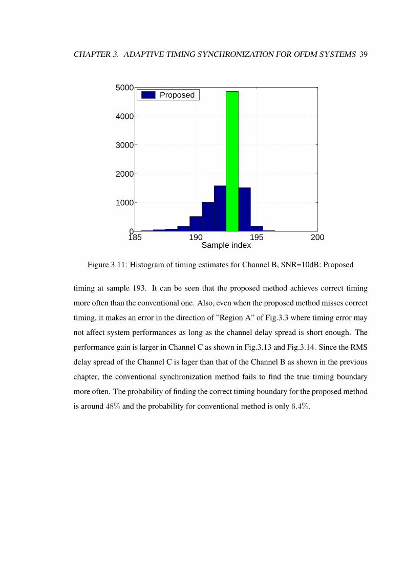
3.11 Histogram of timing estimates for Channel B, SNR=10dB: Proposed . . . . 39
3.12 Histogram of timing estimates for Channel B, SNR=10dB: Conventional . . 40
3.13 Histogram of timing estimates for Channel C, SNR=10dB: Proposed . . . . 40
3.14 Histogram of timing estimates for Channel C, SNR=10dB: Conventional . . 41
4.1 SNR degradation due to RFO . . . . . . . . . . . . . . . . . . . . . . . . . 47
4.2 64-QAM signal constellation without RFO . . . . . . . . . . . . . . . . . . 48
4.3 64-QAM signal constellation with RFO . . . . . . . . . . . . . . . . . . . 48
4.4 Comparison of phase error for ε = 0.01: ML . . . . . . . . . . . . . . . . . 50
4.5 Comparison of phase error : Kalman . . . . . . . . . . . . . . . . . . . . . 55
4.6 Average packet error rate for 4-QAM without channel estimation error (ε =
0.1) . . . . . . . . . . . . . . . . . . . . . . . . . . . . . . . . . . . . . . 58
4.7 Average packet error rate for 64-QAM without channel estimation error
(ε = 0.05) . . . . . . . . . . . . . . . . . . . . . . . . . . . . . . . . . . . 58
4.8 Average packet error rate for 4-QAM (ε = 0.1) . . . . . . . . . . . . . . . 59
4.9 Average packet error rate for 64-QAM (ε = 0.05) . . . . . . . . . . . . . . 59
4.10 Error variance of RFO estimation (ε = 0.1) . . . . . . . . . . . . . . . . . 60
5.1 Block diagram of DFT-based method . . . . . . . . . . . . . . . . . . . . . 64
5.2 Existence of virtual subcarriers . . . . . . . . . . . . . . . . . . . . . . . . 65
5.3 Kalman filtering and smoothing output, SNR=10dB . . . . . . . . . . . . . 68
5.4 MSE comparison in Channel A . . . . . . . . . . . . . . . . . . . . . . . . 73
5.5 SER comparison in Channel A . . . . . . . . . . . . . . . . . . . . . . . . 73
5.6 MSE comparison in Channel B . . . . . . . . . . . . . . . . . . . . . . . . 74
5.7 SER comparison in Channel B . . . . . . . . . . . . . . . . . . . . . . . . 75
xiii

6.1 Block diagram of the simulated BIC-OFDM system . . . . . . . . . . . . . 80
6.2 Timing of successful frame transmission . . . . . . . . . . . . . . . . . . . 83
6.3 Timing of frame transmission failure . . . . . . . . . . . . . . . . . . . . . 83
6.4 Flow chart for iterative procedure for finding power distribution for mini-
mizing packet error rate . . . . . . . . . . . . . . . . . . . . . . . . . . . . 85
6.5 An exemplary plot of constellation size variation with respect to time . . . . 88
6.6 Throughput comparison for improved inner receiver: Channel A & B . . . . 90
6.7 Throughput comparison for conventional system : Channel A & B . . . . . 91
6.8 Throughput comparison for adaptive transceiver in Channel A & B . . . . . 93
6.9 Throughput comparison for adaptive transceiver in Channel A & B . . . . . 94
6.10 Throughput comparison for only adaptive transceiver in Channel A & B . . 95
xiv

Chapter 1
Introduction
Wireless communication has gained a momentum in the last decade of the 20th century
with the success of 2nd Generations (2G) of digital cellular mobile services. Worldwide
successes of GSM, IS-95, PDC, and IS-54/137 are of the few examples demonstrating the
advancement of wireless communications and applications. These systems have initiated
an innovative way of life for the new information and communication technology era. The
total number of cellular subscribers was more than 3 billion in 2007 and now is expected
to exceed approximately 4 billion in 2009. In addition, many of these new subscribers
have started using a number of different forms of data services as well as voice services.
Increasing user demands have drawn the industry to search for better solutions to support
data rates in the range of tens of Mbps. This motivated researchers towards finding a better
solution for handling the nature of wireless channels and limited resources such as power
and bandwidth.
The idea of using multi-carrier transmission for high data rate communications has sur-
faced recently in order to overcome the hostile environments of wireless channels. OFDM
is a special form of multi-carrier transmission where all the subcarriers are orthogonal to
each other. OFDM promises a higher user data rate and greater resilience to severe signal
fading effects of the wireless channel at a reasonable level of implementation complexity.
1

CHAPTER 1. INTRODUCTION 2
Bit & PowerAllocation
OFDMModulator
ChannelInner
ReceiverOuter
ReceiverEncoder
Interleaver
Timing Synchronization Frequency Offset Estimation Channel Estimation
Figure 1.1: Block diagram of an OFDM transceiver
OFDM has developed into a popular scheme for wideband digital communication, whether
wireless or over copper wires, and has been used in applications such as digital television,
audio broadcasting, wireless networking, and broadband internet access. In addition, wire-
less communication has utilized OFDM as the primary physical layer technology in high
data rate Wireless LAN/MAN standards. For example, IEEE 802.11a has the capability to
operate in a range of a few tens of meters in typical office space environment whereas IEEE
802.16a uses Wideband OFDM (W-OFDM), a patented technology of Wi-LAN, to serve
up to 1 km radius of high data rate fixed wireless connectivity. Furthermore, OFDM may
become the prime technology for 4G. Pure OFDM or hybrid OFDM will be most likely the
choice for physical layer technology in future generations of telecommunications systems.
1.1 Why OFDM?
A simplified OFDM transceiver system is described in Fig. 1.1. In a digital domain, binary
input data are collected and FEC coded with schemes such as convolutional codes. The
coded bit stream is interleaved to obtain diversity. Afterwards, a group of channel coded
bits are gathered together (1 for BPSK, 2 for QPSK, 4 for QPSK, etc.) and mapped to
corresponding constellation points. At this point, the IFFT operation is performed on the
parallel complex data and a cyclic prefix is inserted in every block of data according to the

CHAPTER 1. INTRODUCTION 3
system specification. Now, the data is OFDM modulated and ready to be transmitted. After
the transmission of an OFDM signal through a wireless channel, an inner receiver performs
carrier frequency synchronization and symbol timing synchronization. After these steps,
an FFT operation is performed and a channel estimate is obtained. At this point, the com-
plex received data are demapped according to the transmission constellation diagram using
inner receiver estimates. Finally, FEC decoding and deinterleaving are used to recover
the originally transmitted bit stream in the outer receiver. In this thesis, we are going to
present solutions for questions about how to improve inner receiver performance and how
to efficiently allocate bit and power across subcarriers.
OFDM can offer several advantages over single carrier communication systems[1].
First of all, it can efficiently handle frequency selective channels. At high data rates, chan-
nel distortion to data transmission is very significant, and it is difficult to fully recover the
transmitted data with a simple receiver. A very complex receiver structure is needed which
makes use of computationally extensive equalization and channel estimation. OFDM can
drastically simplify the equalization problem by turning the frequency selective channel
into a flat channel. A simple one-tap equalizer is needed to estimate the channel and recover
the data. In addition, in a relatively slow time-varying channel, OFDM can significantly
improve capacity by adapting data rate across subcarriers. This is very useful for multi-
media communications. Furthermore, OFDM is robust against narrowband interference
because such interference affects only a small percentage of the subcarriers. Lastly, OFDM
makes single-frequency networks possible, which is especially attractive for broadcasting
applications.
1.2 Research Challenges
The radio channel has a crucial impact on the transmission of information through it. Multi-
path propagation will occur during a significant part of the time and this causes a frequency

CHAPTER 1. INTRODUCTION 4
Sub-carrier
magnitude
Carrier
Channel
Figure 1.2: OFDM as a broadband communication system
and time selective behavior of the channel response. As the phenomena are random, chan-
nel models for the linear time-variant radio channels are required to estimate the perfor-
mance of radio links and radio networks.
Also, if there are some estimation errors in carrier frequency or symbol timing, it will
induce significant errors in communication. The success of wireless OFDM system de-
pends strongly on synchronization. The higher the data rates are, the stricter the synchro-
nization requirements become. In order to build systems to support higher and higher data
rates, there is a need for algorithms and system designs that can facilitate robust estimation
of the synchronization parameters with minimum computational complexity.
Channel estimation is another primary requirement of an OFDM transceiver that per-
forms coherent reception. The capacity of a system is largely dependent on the channel
estimation scheme used in the system. The more accurate the channel estimate is, the bet-
ter the quality of service. OFDM offers a built-in very simple frequency domain channel
estimation scheme. Despite the fact that the scheme is simple enough, it does not perform
accurately under very low SNR conditions.
In 802.11a, the link adaptation algorithm is intentionally left open. Although many
previous studies have been focused on this particular topic, many of them are not directly
applicable to real systems. In addition, the actual optimization benefit that can be realized

CHAPTER 1. INTRODUCTION 5
after taking into account complexity always remains a question.
This dissertation explores the applicability of statistical estimation and optimization
techniques to the above mentioned problems in OFDM systems. Using 802.11a as an ex-
ample, we analyze the effect of various estimation errors and propose novel methods to mit-
igate synchronization and channel estimation error with reasonable complexity. Moreover,
we introduce a simple method to improve throughput performance by adaptively chang-
ing constellation size and power distribution across the sub-carriers without sacrificing
throughput due to explicit feedback. By employing the proposed scheme, we examine
the value of optimization with practical impairments.
1.3 Outline of the Thesis
Chapter 1 is a brief introduction and motivation. Chapter 2 considers an indoor wireless
channel model. An indoor wireless channel is always very unpredictable with harsh and
challenging propagation conditions. Measurement results show that an indoor wireless
channel is very different from a mobile channel in many ways. We particularly focused on
a delay spread model in this study and propose a new model for Doppler power spectrum
for an indoor channel. These models in Chapter 2 will be the basis for our discussion on
how we can improve the current systems in later chapters.
Adaptive timing synchronization for frequency selective channels is studied in Chapter
3. In burst packet mode OFDM systems, timing synchronization need to be done within a
single training symbol time to avoid reduction of the system capacity. Due to this stringent
requirement on synchronization time, standards incorporate preambles suitable for corre-
lation to estimate symbol timing. However, in time-dispersive multi-path channels, the
conventional timing synchronization methods might synchronize to a path in the middle
of the overall channel impulse response (CIR). Consequently, the receiver may not capture
some of the multi-path components. This results in an inter-symbol interference (ISI) and

CHAPTER 1. INTRODUCTION 6
an inter-carrier interference (ICI). In this chapter, we present a novel timing synchroniza-
tion method for OFDM systems to detect the most significant channel taps by adaptively
changing observation window length. The method does not require any extra channel infor-
mation such as signal to noise ratio (SNR) or average power delay profile, while allowing
detection of the first arrived path position. Additionally estimating maximum delay spread
and total channel power can be used to increase system capacity in other applications.
Chapter 4 moves on to a residual frequency offset and phase tracking problem. In
OFDM systems, carrier frequency offset (CFO) due to mismatch of the local oscillators
causes ICI, which may result in significant performance degradation. Although, several
frequency synchronization schemes were reported in the past, there can remain frequency
offset and that can still generate ICI and induce phase distortion of the OFDM symbols.
In this chapter, we propose a method to compensate both residual frequency offset (RFO)
and RFO induced phase error (PE) for OFDM systems by using the Kalman filter. In our
proposed method, the linear state-space model for RFO and PE is derived using estimated
SNR. After building a state-space model, the Kalman filter is applied to track and estimate
RFO and PE simultaneously. The proposed method allows unknown parameters to evolve
in time due to frequency drift of the local oscillator. The method is an optimal linear
estimator assuming signal and noise are jointly Gaussian. Furthermore, the computation
cost of the proposed method is much lower than that of the LS phase fitting method due to
the small dimension of the state-space model.
Chapter 5 also considers another estimation problem in an OFDM inner receiver. In
practical OFDM systems with virtual carriers (VCs), conventional DFT-based approaches
are not directly applicable for channel estimation as they induce a spectral leakage owing
to the VCs. This results in an error floor for the mean square error (MSE) performance. To
circumvent this problem, we propose an enhanced DFT-based minimum mean square error
(MMSE) channel estimator using the Kalman smoother. Our approach is based on building
a robust state-space model for a channel frequency response (CFR). Kalman filtering and

CHAPTER 1. INTRODUCTION 7
smoothing is then applied to minimize the leakage effect. Time domain MMSE weighting
is also used to suppress the channel noise. This proposed method does not require extra
knowledge about the channel statistics and can be implemented with small complexity
while achieving similar performance to the optimal MMSE estimation.
As we mentioned above, OFDM in combination with bit-interleaved coded modula-
tion is an efficient and robust high-speed transmission technique used in the IEEE 802.11a
standard. In Chapter 6, using the request to send (RTS)/ clear to send (CTS) mechanism,
we present a throughput enhancement method by deriving a simplified expression for the
throughput in the 802.11a system. The IEEE 802.11 MAC specifies for the contention-
based distributed coordination function (DCF) access method to exchange short control
frames - RTS/CTS prior to data transmission. RTS/CTS handshaking is essentially a
medium reservation scheme, and this mechanism is one of the effective ways to alleviate the
hidden node problem under DCF. Assuming channel reciprocity, we incorporate this mech-
anism for getting channel information at the transmitter without sacrificing throughput due
to explicit feedback. After acquiring channel knowledge, a simple iterative algorithm is
used to select constellation sizes and power distribution across the sub-carriers to enhance
the throughput.
As a conclusion, we review the results we have obtained and present some ideas for
future research in Chapter 7 and conclude this thesis.

Chapter 2
Indoor Wireless Channel
Due to the nature of wireless communications, wireless channels have very different char-
acteristics from wire-line channels. The mechanisms which govern radio propagation are
complex and diverse, and they can generally be attributed to three basic propagation mech-
anism as follows: reflection, diffraction and scattering. One of the most important charac-
teristics of a multi-path channel is the time varying nature of the channel which is called
small-scale variation. This time variation occurs because of the movement of the transmit-
ter or the receiver or the location of the obstacles.
In this chapter, we describe small scale fading characteristics of wireless channels
which are suitable for describing indoor wireless communication. We then give a brief
overview of European Telecommunications Standards Institute (ETSI) channel models and
propose a new autocorrelation model for temporal variation of an indoor wireless channel.
It is important to understand the different characteristics and properties of indoor wire-
less channels because the measurements of indoor channels show distinct differences from
mobile channel measurements.
8
CHAPTER 2. INDOOR WIRELESS CHANNEL 9
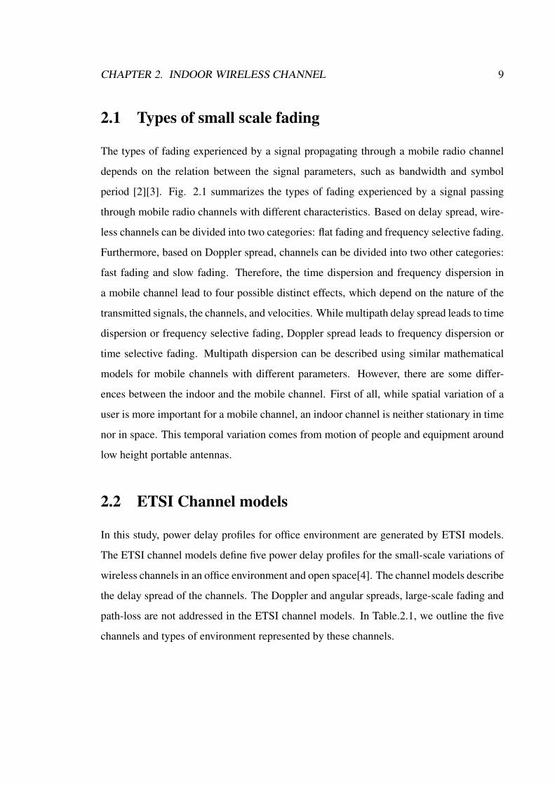
2.1 Types of small scale fading
The types of fading experienced by a signal propagating through a mobile radio channel
depends on the relation between the signal parameters, such as bandwidth and symbol
period [2][3]. Fig. 2.1 summarizes the types of fading experienced by a signal passing
through mobile radio channels with different characteristics. Based on delay spread, wire-
less channels can be divided into two categories: flat fading and frequency selective fading.
Furthermore, based on Doppler spread, channels can be divided into two other categories:
fast fading and slow fading. Therefore, the time dispersion and frequency dispersion in
a mobile channel lead to four possible distinct effects, which depend on the nature of the
transmitted signals, the channels, and velocities. While multipath delay spread leads to time
dispersion or frequency selective fading, Doppler spread leads to frequency dispersion or
time selective fading. Multipath dispersion can be described using similar mathematical
models for mobile channels with different parameters. However, there are some differ-
ences between the indoor and the mobile channel. First of all, while spatial variation of a
user is more important for a mobile channel, an indoor channel is neither stationary in time
nor in space. This temporal variation comes from motion of people and equipment around
low height portable antennas.
2.2 ETSI Channel models
In this study, power delay profiles for office environment are generated by ETSI models.
The ETSI channel models define five power delay profiles for the small-scale variations of
wireless channels in an office environment and open space[4]. The channel models describe
the delay spread of the channels. The Doppler and angular spreads, large-scale fading and
path-loss are not addressed in the ETSI channel models. In Table.2.1, we outline the five
channels and types of environment represented by these channels.

CHAPTER 2. INDOOR WIRELESS CHANNEL 10
Figure 2.1: Two types of small scale fading
Table 2.1: ETSI channel modelsChannel RMS delay spread Environment LOS/NLOS
A 50ns Typical office NLOSB 100ns large open space and office NLOSC 150ns large open space NLOSD 140ns large open space LOSE 250ns large open space NLOS

CHAPTER 2. INDOOR WIRELESS CHANNEL 11
0 0.1 0.2 0.3 0.40
5
10
15
20
25
30
Delay spread (µ s)
Pow
er (
−dB
)
(a) ETSI Channel A
0 0.2 0.4 0.6 0.80
5
10
15
20
25
Delay spread (µ s)
Pow
er (
−dB
)
(b) ETSI Channel B
Figure 2.2: Power delay profile for channel A and B

CHAPTER 2. INDOOR WIRELESS CHANNEL 12
0 0.5 1 1.50
5
10
15
20
25
Delay spread (µ s)
Pow
er (
−dB
)
(a) ETSI Channel C
0 0.5 1 1.5 20
5
10
15
20
25
Delay spread (µ s)
Pow
er (
−dB
)
(b) ETSI Channel E
Figure 2.3: Power delay profile for channel C and E

CHAPTER 2. INDOOR WIRELESS CHANNEL 13
Since Channel C and D have the same power delay profile, the power delay profile for
only Channel A, B, C and E are shown Fig.2.2 and Fig.2.3. From the power delay profile
of channel A in Fig.2.2, we can observe that the maximum delay spread is about 0.4 µ
secs and the power delay profile consists of two clusters of exponentially decaying paths.
Another point worth noticing is the first arrived path for the profile is not the strongest one
except in Channel A. This effect on timing synchronization will be discussed in the next
chapter. We also observe that the maximum delay spread increases from Channels B to
C to E. This increase in frequency selectivity not only increases diversity gains but also
implies an increase in intersymbol interference (ISI). ISI occurs when delayed copies of a
transmitted symbol overlap the next transmitted symbol and usually degrades the perfor-
mance of wireless systems. In addition, while the power delay profiles for Channels C and
D are the same, there is a line of path (LOS) with power of about 10dB higher than the
sum of average power of all paths in the power delay profile for Channel D. Consequently,
the frequency selectivity of the two channels are the same but Channel D is more stable
due to the non-faded path. Therefore, a system in Channel D would perform better than in
Channel C and, hence, Channel D will not be used in this study.
2.3 Modeling the Time Varying Channel
The fading characteristics of indoor wireless channels are very different from the previously
reported mobile cases. However, in indoor wireless systems, the transmitter and receiver
are stationary and people are moving in between, whereas in outdoor mobile systems, the
user is moving through an environment. Although, this sort of time variation has been
observed in the literatures, for example [5] and [6], it is not thoroughly analyzed yet. A
stochastic time variation model was proposed for fixed wireless communication [7]. How-
ever, numerical methods are needed to implement this model and an inclusion of numerical
components will cause additional delay in practical simulations. In this section, we extend

CHAPTER 2. INDOOR WIRELESS CHANNEL 14
the method of [7] and derive a closed form stochastic channel model for an indoor wireless
communication simulation.
2.3.1 Mobile Radio Channel
The complex baseband representation of a wireless channel impulse response can be de-
scribed as,
h(t, τ) =∑
n
αn(t)e−jφn(t)δ(τ − τn(t)) (2.1)
where τn(t) is the delay of the nth path and αn(t) is its real amplitude. Due to the motion
of the user, αn(t)e−jφn(t) represents a wide-sense stationary narrowband complex Gaussian
process, which is independent for different path. If the user moves at speed v in the direc-
tion of θ as shown in Fig. 2.4, The phase change of a ray due to the moving receiver can be
easily obtained as
φ(t + ∆t)− φ(t) = 2πfcv
c∆t cos θ (2.2)
Therefore, assuming the power of each incident wave is uniformly distributed, the corre-
sponding autocorrelation function and Doppler power spectrum for nth tap are [3],
R(∆t) = E[exp(φ(t + ∆t)− φ(t))]
=1
2π
∫ 2π
0
exp(j2πfcv
c∆t cos θ)dθ
= J0
(2π
fcv
c∆t
)(2.3)
where fc is the carrier frequency. Fourier transforming above equation, we can derive
power spectrum as,

CHAPTER 2. INDOOR WIRELESS CHANNEL 15
Receiver
Incident Plane Wave
Figure 2.4: Illustration of Doppler shift
S(f) =1
π√
f 2d − f 2
(2.4)
where fd denotes Doppler frequency and c is the speed of light. This model is called the
Jake’s model [45] and widely accepted for cellular environments where spatial variation
is more important than temporal variation. However, it deviates from measured Doppler
spectra in indoor wireless channel environments.

CHAPTER 2. INDOOR WIRELESS CHANNEL 16
Transmitter Receiver
Reflector
Figure 2.5: Geometry of a single ray
2.3.2 Indoor Wireless Channel
Fig. 2.5 shows the case when the transmitter and receiver are stationary and reflectors are
moving in the direction of θ at speed v. The phase change of a ray due to a moving reflector
can be easily obtained as [7],
φ(t + ∆t)− φ(t) = 4πfcv
c∆t cos θ cos ψ (2.5)
Assuming all reflectors are moving in a similar manner and the power of each incident
wave is uniformly distributed, the autocorrelation function and Doppler power spectrum
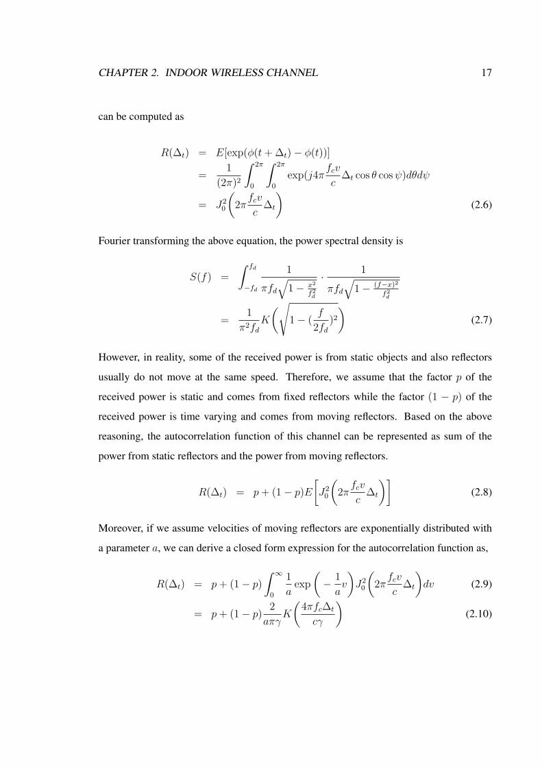
CHAPTER 2. INDOOR WIRELESS CHANNEL 17
can be computed as
R(∆t) = E[exp(φ(t + ∆t)− φ(t))]
=1
(2π)2
∫ 2π
0
∫ 2π
0
exp(j4πfcv
c∆t cos θ cos ψ)dθdψ
= J20
(2π
fcv
c∆t
)(2.6)
Fourier transforming the above equation, the power spectral density is
S(f) =
∫ fd
−fd
1
πfd
√1− x2
f2d
· 1
πfd
√1− (f−x)2
f2d
=1
π2fd
K
(√1− (
f
2fd
)2
)(2.7)
However, in reality, some of the received power is from static objects and also reflectors
usually do not move at the same speed. Therefore, we assume that the factor p of the
received power is static and comes from fixed reflectors while the factor (1 − p) of the
received power is time varying and comes from moving reflectors. Based on the above
reasoning, the autocorrelation function of this channel can be represented as sum of the
power from static reflectors and the power from moving reflectors.
R(∆t) = p + (1− p)E
[J2
0
(2π
fcv
c∆t
)](2.8)
Moreover, if we assume velocities of moving reflectors are exponentially distributed with
a parameter a, we can derive a closed form expression for the autocorrelation function as,
R(∆t) = p + (1− p)
∫ ∞
0
1
aexp
(− 1
av
)J2
0
(2π
fcv
c∆t
)dv (2.9)
= p + (1− p)2
aπγK
(4πfc∆t
cγ
)(2.10)

CHAPTER 2. INDOOR WIRELESS CHANNEL 18
where a is mean velocity of the moving reflectors, K is the complete elliptic integral and
γ =√
1a2 + 4(2π fc
c∆t)2. Once we have an autocorrelation function, we can generate a ran-
dom process of the channel by spectrum filtering or spectrum sampling [3] and implement
a multipath fading simulator.
The Doppler power spectra and the autocorrelation functions for different environments
are shown in Fig.2.6 and Fig.2.7. The dotted line corresponds to the Jake’s model when a
receiver is moving at 4km/h and the dashed line, referred to as the worst case, represents the
case when p is zero and all reflectors are moving at 4km/h. Finally, the solid line represents
the proposed model when p is zero and a is 4km/h. Note that the proposed model gives
rise to more peaky Doppler spectrum and has wider spread of the power spectrum than the
Jake’s model in the frequency domain. Also, the autocorrelation function of the proposed
model shows less oscillatory behavior than that of the Jake’s model in the time domain.
Fig.2.8 shows a comparison between an indoor channel measurement result in [8] and
the proposed model. p and a are set to be 0.97 and 8km/h respectively and the power
spectral density of the proposed model is normalized to have the same received power
as the measurement. We can see that the proposed model matches the indoor channel
measurement well. In addition, it can be seen that the Jake’s model can not be fitted to this
measurement regardless of fd. Consequently, the proposed model can be used for more
accurate simulations of indoor wireless channels than the Jake’s model. In addition, since
the proposed model has a closed form expression, it has a lower computational complexity
than the model in [7]. This time variation model will be used throughout this dissertation.

CHAPTER 2. INDOOR WIRELESS CHANNEL 19
−2 −1 0 1 2−30
−25
−20
−15
−10
−5
Normalized frequency
Mag
nitu
de (
dB)
Jakes modelWorst caseExponentional model with p=0
Figure 2.6: Doppler power spectrum
0 0.05 0.1 0.15 0.2−0.5
0
0.5
1Jakes modelWorst caseExponentional model with p=0
Figure 2.7: Autocorrelation function

CHAPTER 2. INDOOR WIRELESS CHANNEL 20
−10 −5 0 5 10−100
−90
−80
−70
−60
−50
−40
−30
Frequency (Hz)
Doppler Power Spectrum
Figure 2.8: Comparison between Doppler spectrum measurement and proposed Dopplerspectrum model

Chapter 3
Adaptive Timing Synchronization for
OFDM Systems
In burst packet mode OFDM systems, timing synchronization needs to be done within a
single training symbol time to avoid reduction of the data throughput. Due to this stringent
requirement on synchronization time, standards incorporate preambles suitable for using
correlation to estimate symbol timing. However, in time-dispersive multi-path channels,
conventional timing synchronization methods may synchronizes to a path in the middle of
the overall channel impulse response (CIR). Consequently, the receiver may not capture
some of the multi-path components. This results in an inter-symbol interference (ISI) and
an inter-carrier interference (ICI). In this chapter, we propose a simple adaptive timing
synchronization method to locate the first arriving path based on the use of one training
symbol in the preamble. Our computer simulation results show that the proposed method
can significantly improve error rate performance. The performance gain becomes higher as
delay spread increases.
21

CHAPTER 3. ADAPTIVE TIMING SYNCHRONIZATION FOR OFDM SYSTEMS 22
3.1 Introduction
In OFDM, the modem can invert dispersive broadband channels into parallel narrow band
sub-channels, thus significantly simplifying equalization at the receiver. However, this
inherent immunity of OFDM to time-dispersive multi-path channels comes at the price of
increased sensitivity to synchronization error. Imperfect synchronization causes ISI and
ICI which can result in significant performance degradation [1] [11].
Several approaches have been proposed on the basis of using training symbols or using
the repetition property of cyclic prefixes [12] [13]. In burst packet mode OFDM systems,
the method using a preamble is preferred for fast time and frequency synchronization due
to the stringent requirement to minimize synchronization time. In [12] and [13], an auto-
correlation based timing metric is calculated. This calculation correlates the received sam-
ples and their delayed copies. These algorithms, based on the auto-correlation, inevitably
result in an ambiguity in timing due to a plateau region and to enhanced sensitivity to burst
noise. This ambiguity must be resolved after the auto-correlation process. One solution
to this problem is to use a cross-correlation method, which correlates the received samples
with known training samples. The cross-correlation peak of the received samples is used
for symbol timing. This method has very good performance in an AWGN environment
but has significant drawbacks since it is sensitive to frequency offset and the power delay
profile of the channel. In [23], short training symbols (STS) are used for timing estimation
via a combination of an auto-correlation and a cross-correlation. However, as mentioned
above, frequency offset in the local oscillator can disturb the cross correlation peaks sig-
nificantly, which will significantly affect the accuracy of the timing estimate. Furthermore,
a few sample errors in the coarse timing estimate may cause significant timing errors in
the resulting fine timing estimate. Therefore, in order to use a cross-correlation method to
estimate timing, frequency offset must be kept small, such as within 50Khz for 802.11a
and HiperLAN/2 environments [18].

CHAPTER 3. ADAPTIVE TIMING SYNCHRONIZATION FOR OFDM SYSTEMS 23
In [19], after coarse frequency offset is compensated, fine timing estimation is done
using the periodic property of long training symbols (LTS). This algorithm, however, makes
no effort to estimate the position of the first arriving multi-path component, leading to an
inefficient utilization of the guard interval in multi-path channels. This also causes ISI
and ICI in the demodulation process. One intuitive solution to this problem is to shift
a few samples in the appropriate direction from the acquired correlation peak position.
However, since neither average nor instantaneous power delay profiles (PDP) of the channel
are available, it is not obvious how many samples should be shifted. In [16], they used a
double auto-correlation method to estimate the timing and the energy of the CIR to find the
first arriving path of the signal which may not be the strongest. However, this method has
a weakness that the timing estimate can be compensated only after channel estimation and
it is also not straightforward to decide the optimal window size, which is dependent on the
delay spread of the channel.
In this chapter, we present an adaptive timing synchronization method for OFDM sys-
tems using burst packet mode. In our proposed method, before symbol timing estimation,
frequency offset is corrected by a typical maximum likelihood (ML) method. Hence, the
cross-correlation based timing estimation accuracy is not affected by frequency offset, and
the cross-correlation output is used to detect the most significant channel taps by adaptively
changing an observation window. The proposed method in this chapter does not require
any extra channel information such as signal to noise ratio (SNR) or PDP, while allowing
detection of the first arriving path position and additionally estimating the maximum de-
lay spread and total channel power which can be used to increase system throughput in
other applications. We evaluate the performance of our method with the 802.11a standard
[9] in four different indoor PDP scenarios [4]. Simulation results show that our proposed
method significantly outperforms conventional peak selection methods and is robust to var-
ious channel environments with practical impairments.

CHAPTER 3. ADAPTIVE TIMING SYNCHRONIZATION FOR OFDM SYSTEMS 24
10 2 3 4 65 7 8 9 GI2 T1 T2
P1 P2 Header Data Data ……. Data
Details of the preamble field
10 short symbols (0.8*10 = 8 s) 2 long symbols (1.6+2*3.2 = 8 s)
Signal detection, AGC, Coarse timing
recovery, Freq. acquisition
Fine timing recovery, Freq. offset
estimation, Channel estimation
8 s 8 s 4 s
4 Pilot sub-carriers for phase tracking
Figure 3.1: 802.11a - Frame and slot structure
3.2 System Model
Fig.3.1 shows an example of OFDM frame and slot structure In the WLAN standard
adopted by the IEEE 802.11a. Each data packet consists of preamble and a payload. The
preamble consist of 10 short training symbols (STS) of length of 16 samples (8µs) and long
training symbols (LTS) of length of 64 samples (8µs) which are all utilized for synchro-
nization and channel estimation. The data carrying part consists of a variable number of
symbols and the length of each data symbol is 64 samples. Note that a short symbol serves
as a cyclic prefix for a subsequent short symbol. For LTS, GI2 is the cyclic prefix for T1
and it contains 32 of the last samples (1.6µs) of T1. In the frequency domain, a data symbol
contains data subcarriers and some known pilot subcarriers that are usually used for phase
tracking. Fig.3.2 shows an example of the subcarrier allocation for the IEEE 802.11a sys-
tem. Out of the 64 possible subcarriers, only 52 subcarriers are used. Of the 52 subcarriers
used, 48 subcarriers are dedicated to data transmission and 4 are pilot subcarriers.
More generally, let’s consider an OFDM system with FFT length N where a total of

CHAPTER 3. ADAPTIVE TIMING SYNCHRONIZATION FOR OFDM SYSTEMS 25
−40 −30 −20 −10 0 10 20 30 40frequency index
Data subcarriersGuard bandPilot subcarriers
Figure 3.2: 802.11a - Subcasrrier allocation
Nu subcarriers are used for transmission. The transmitted signal s(n) is generated by an
IFFT of data symbols Ak and a guard interval of length Tg = Ng · Ts is placed in front of
the useful portion Tu = N · Ts of the signal to prevent ISI. Ts denotes the sampling time
period. Then
s(n) =1
N
Nu/2+1∑
k=−Nu/2
Ak · expj2πnk
N(3.1)
for −Ng ≤ n ≤ N − 1
The baseband impulse response of the channel is assumed to be in the form of
h(n) =L−1∑
l=0
h(l)δ(n− l) (3.2)
where L is the maximum delay spread of the channel and h(l) represents the complex gain
of the lth multi-path component. Assume time invariance over one OFDM symbol. After

CHAPTER 3. ADAPTIVE TIMING SYNCHRONIZATION FOR OFDM SYSTEMS 26
transmission over this multi-path channel, the samples at the receiver are
r(n) =L−1∑
l=0
s(n− l − nt) · h(l) · exp (j2πεn
N+ θ) + N(n) (3.3)
where N(n) is complex white Gaussian noise at time n, nt = δt/Ts is the timing offset, θ is
an unknown phase and ε = NTs ·δf is the normalized carrier frequency offset. If the guard
interval is correctly removed, the signal is then demodulated by FFT resulting in output at
the subcarrier k of
Yk = Hk · Ak + Nk (3.4)
for −Nu/2 ≤ k ≤ Nu/2 + 1 (3.5)
As long as the start position of the FFT window is in the ”Region A” in Fig.3.3, no
ISI or ICI occurs. Changing the start position will only induce phase rotation across the
subcarriers and this rotation can not be distinguished from actual channel phase response
so performance degradation does not occur. However, if the FFT start position is in the
”Region B”, it will cause ISI and ICI [15]. This effect is minimized when the energy of the
channel inside the guard interval of Ng in Fig.3.3 is the maximum.
In the presence of timing estimation error, the post FFT signal can be derived as
Yk = Hk · Ak · α(nt) + Nk + Nnt,k (3.6)
for −Nu/2 ≤ k ≤ Nu/2 + 1
Attenuation, α(nt), can usually be neglected for large N , so the main disturbance comes
from additional noise, Nnt,k. It was shown that this noise can be approximated by Gaussian

CHAPTER 3. ADAPTIVE TIMING SYNCHRONIZATION FOR OFDM SYSTEMS 27
N Ng
B A B
FFT Window
L
FFT Start Position
Channel Response
Figure 3.3: Timing synchronization diagram
noise with power [14],
σ2nt
=∑
i
|hi|2(2 · g(nt)− g(nt)2) (3.7)
where g is a linear function depending on relative timing offset. Furthermore, a timing
offset will have another effect on the performance. Since some portion of the effective
channel is shifted, this portion can not contribute to the channel estimate. The resulting
channel estimation error is given by [24],
σ2c = E[|Hk −H∆,k|2] =
Nsu
N
∑i∗|hi∗ |2 (3.8)
SNR′ ≈ f 2
N(ε) · SNR(1− f 2
N(ε)) · SNR · (N/Nsu) + 1(3.9)
fN(ε) =sin(πε)
N sin(πε/N)

CHAPTER 3. ADAPTIVE TIMING SYNCHRONIZATION FOR OFDM SYSTEMS 28
3.3 Frequency and Timing Synchronization
The proposed method can be broken into two steps. In order to use a cross-correlation
based timing synchronization method, frequency offset is compensated first using STS.
After successful frequency offset compensation, the FFT start position is found by our
proposed timing synchronization method.
3.3.1 Coarse Frequency Offset Estimation
STS are periodic after Ns samples. Then ML estimate of frequency offset can be obtained
by auto-correlation of the received signal.
A(n) =Wa−1∑m=0
r(n + m)r∗(n + m + Ns) (3.10)
ε =−N
2πNs
· tan−1(A(n)) (3.11)
where Ns = 16 for 802.11a [9], Ns = 64 for 802.16a [10] and Wa is the averaging length
which is dependent on the automatic gain control (AGC). During the AGC stabilization
time, the received signal will be corrupted by large gain fluctuations that cause the auto-
correlation output to be unstable. For most AGC systems, this process will last for the
first 48-80 samples of the STS [20]. Therefore, Wa is set to be less than 4 STS periods
for 802.11a systems. Using the method in [21], acquisition range and Cramer-Rao lower
bounds (CRLB) can be obtained as,
|ε| ≤ N
2Ns
(3.12)
var(ε) ≥ (N
2π · ks ·Ns
)2 · 1
Ns · SNR(3.13)

CHAPTER 3. ADAPTIVE TIMING SYNCHRONIZATION FOR OFDM SYSTEMS 29
where ks is the number of STS such that Wa = ks · Ns and SNR is defined as E[|r(n) −n(n)|2]/E[|n(n)|2]. After symbol timing is acquired as described in the next section, the
LTS are used to further reduce the frequency offset estimation error. For this case, Ns is set
to be the length of the LTS, NL, and ks is set to be 1.
3.3.2 Adaptive Timing Synchronization method
After the packet detection algorithm signals the start of the packet, the symbol timing
algorithm refines the timing estimation to a sample period precision. This is conventionally
done by using the cross-correlation between the received signal r(n) and a known reference
tn with length NL. The reference, tn, can be made by concatenating last NL/2 samples of a
LTS with the first NL/2 samples of a LTS. The value of n that corresponds to the maximum
absolute value of the cross-correlation in (3.14) is the symbol timing estimate.
Tf = arg maxn
(|NL−1∑m=0
r(n + m)t∗m|2) (3.14)
tn = [LNL/2:NLL0:NL/2−1] (3.15)
where NL = 64 for 802.11a, NL = 128 for 802.16a. If the first arriving path is the strongest
path, this conventional method can detect the boundary between the last STS and the first
LTS, which is n = 161. Since the guard interval for the LTS is 32 samples, the exact FFT
start position, n = 193, can be found. But the conventional method that is mentioned above
fails to find true FFT start position if the first arriving path is not the strongest path. In such
cases , cross-correlation may take the highest correlation value associated with the path that
arrives later than the first path and this may result in severe ISI and ICI.
In order to avoid this problem, we utilize the fact that the cross-correlation output ap-
proximately coincides with scaled instantaneous channel power. Suppose C(n) is defined
as a cross-correlation output. The conditional expectation of C(n), given h(n), is obtained

CHAPTER 3. ADAPTIVE TIMING SYNCHRONIZATION FOR OFDM SYSTEMS 30
as the following equation when a multi-path component exists at index n:
E[C(n)|h(n)] = E[|NL−1∑m=0
r(n + m)t∗m|2|h(n)] (3.16)
= |h(n)|2(Nu
N)2 + σ2
n
Nu
N+ σ2
I (3.17)
However, if a multi-path component does not exist at index n, the above equation be-
comes
E[C(n)|h(n)] = σ2n
Nu
N+ σ2
I (3.18)
where the number of used subcarriers, Nsu, is 52 for 802.11a and σI is additional
noise due to the imperfect cross-correlation property of the pseudo random sequence in
the preamble.
Let us define D(n) and QW (n) as
D(n) = C(n)− σ2n
Nu
N− σ2
I (3.19)
QW (n) =W−1∑m=0
D(n + m) (3.20)
where W is a summation window length. The QW (n) represents a normalized summation
of W consecutive samples of C(n). Also, the conditional expectation of QW (n) is zero
if a multi-path component does not exist within summation interval, W . Fig.3.4 shows an
exemple plot of D(n) when the maximum channel length is five sample periods.
As long as the window length, W , is greater than the maximum delay spread of the
channel, the maximum of QW (n) does not change except for some fluctuation due to noise.
Meanwhile, if the window length becomes less than the maximum delay spread of the

CHAPTER 3. ADAPTIVE TIMING SYNCHRONIZATION FOR OFDM SYSTEMS 31
W
Figure 3.4: Exemplary plot of D(n) at SNR=10dB

CHAPTER 3. ADAPTIVE TIMING SYNCHRONIZATION FOR OFDM SYSTEMS 32
Max delay spread = 4
Figure 3.5: QW output when W = 16, 8, 4 and 3

CHAPTER 3. ADAPTIVE TIMING SYNCHRONIZATION FOR OFDM SYSTEMS 33
channel, the maximum of QW (n) will be significantly decreased. Therefore, the position of
the first arriving path can be estimated by detecting a significant decrease of the maximum
of QW (n). However, since the noise fluctuation of the maximum of QW (n) could lead to
an incorrect timing estimate, QW , which is defined as the average of the samples whose
magnitudes are greater than 90% of the maximum of QW (n), is used for timing estimation
instead of the maximum of QW (n). Suppose the window size W ∗ and the 90% maximum
start decreasing more than ξ%. Then it can be seen that arg maxn(QW ∗+1(n)) corresponds
to the first arriving path position since it indicates the starting time of the window which
contains the maximum power of the CIR. For example, Fig.3.5 represents QW (n) output
when {W = 16, 8, 4, 3} according to the D(n) in Fig.3.4. Since QW (n) starts decreasing
when W ∗ = 3, the resulting timing estimate can be obtained from arg maxn(QW ∗+1(n)) =
193. If we used the conventional peak-detection method, the resulting timing estimate
would be n = 196. The above method can be executed by a binary search algorithm with
high efficiency. It also can provide an estimate of the instantaneous maximum delay spread,
W ∗ + 1 and an estimate of the instantaneous total channel power.
The proposed method is summarized below:
1. Compensate frequency offset ε by (3.11).
2. Calculate C(n) and D(n).
3. Execute binary search algorithm to find W ∗ using initial W = Ng.
4. Declare timing estimate as arg maxn(QW ∗+1(n)).
CHAPTER 3. ADAPTIVE TIMING SYNCHRONIZATION FOR OFDM SYSTEMS 34
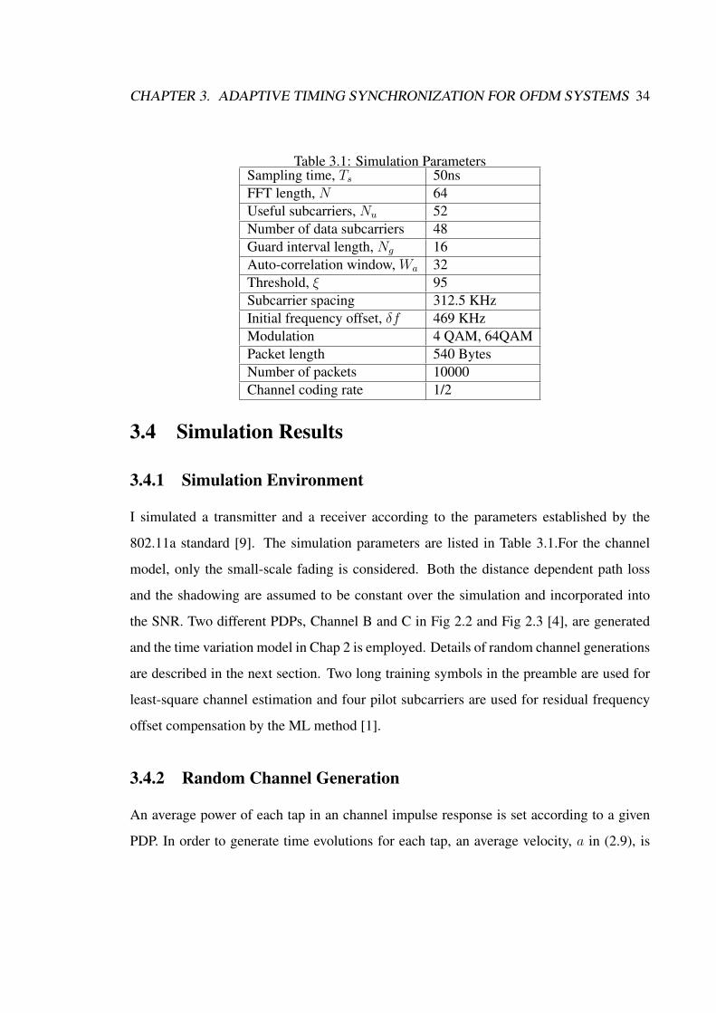
Table 3.1: Simulation ParametersSampling time, Ts 50nsFFT length, N 64Useful subcarriers, Nu 52Number of data subcarriers 48Guard interval length, Ng 16Auto-correlation window, Wa 32Threshold, ξ 95Subcarrier spacing 312.5 KHzInitial frequency offset, δf 469 KHzModulation 4 QAM, 64QAMPacket length 540 BytesNumber of packets 10000Channel coding rate 1/2
3.4 Simulation Results
3.4.1 Simulation Environment
I simulated a transmitter and a receiver according to the parameters established by the
802.11a standard [9]. The simulation parameters are listed in Table 3.1.For the channel
model, only the small-scale fading is considered. Both the distance dependent path loss
and the shadowing are assumed to be constant over the simulation and incorporated into
the SNR. Two different PDPs, Channel B and C in Fig 2.2 and Fig 2.3 [4], are generated
and the time variation model in Chap 2 is employed. Details of random channel generations
are described in the next section. Two long training symbols in the preamble are used for
least-square channel estimation and four pilot subcarriers are used for residual frequency
offset compensation by the ML method [1].
3.4.2 Random Channel Generation
An average power of each tap in an channel impulse response is set according to a given
PDP. In order to generate time evolutions for each tap, an average velocity, a in (2.9), is

CHAPTER 3. ADAPTIVE TIMING SYNCHRONIZATION FOR OFDM SYSTEMS 35
Time
Delay
Packetduration
Figure 3.6: A time variation technique for simulation
set to 4km/h. After obtaining a Doppler power spectrum, S(f), as described in Chap 2, a
spectrum sampling method [3] is used to independently generate time domain samples for
each tap. Consequently, the baseband representation of a channel impulse response at the
kth tap is,
hk(t) =∑N
n=1
√S(fn) · e−j(2πfnt+φn)
where S(·) is a Doppler power spectrum in Chap 2 and φn are random phases on [0, 2π].
Since the channel variation between adjacent two OFDM symbols are small, only two time
samples are generated for a tap inside a packet. The two time samples are chosen to be the
beginning and the ending time of a packet. A time variation inside these two time samples
is obtained by a linear interpolation as shown in Fig.3.6.

CHAPTER 3. ADAPTIVE TIMING SYNCHRONIZATION FOR OFDM SYSTEMS 36
6 8 10 12 14 16 1810
−2
10−1
100
Average SNR (dB)
Ave
rage
pac
ket e
rror
rat
e
ProposedConvIdeal
Figure 3.7: Average packet error rate for 4QAM in Channel B
3.4.3 Performance Results
Fig.3.7 - Fig.3.10 show average packet error rate for the proposed method in two differ-
ent delay spread environments. The ordinate represents average packet error rate and the
abscissa represents average SNR. ”Ideal” is the case when ideal timing estimation is avail-
able and ”Conv” is the case when the peak location of the cross-correlation is declared
as the FFT start position. As you can see from the figures, the proposed method method
significantly outperforms the conventional method in all scenarios. This result is expected
from the PDP of the channel since the conventional method tends to be synchronized to a
path in the middle of the overall CIR. The probability that the first arriving path becomes
the strongest path is low for these channels. With incorrect timing estimate, the conven-
tional method experiences ISI and ICI and these interference become larger as the delay
spread increases finally leading to an error floor and this effect is more critical as modu-
lation complexity increases. The performance improvement in the proposed method over

CHAPTER 3. ADAPTIVE TIMING SYNCHRONIZATION FOR OFDM SYSTEMS 37
18 20 22 24 26 28 3010
−2
10−1
100
Average SNR (dB)
Ave
rage
pac
ket e
rror
rat
e
ProposedConvIdeal
Figure 3.8: Average packet error rate for 64QAM in Channel B
6 8 10 12 14 16 1810
−2
10−1
100
Average SNR (dB)
Ave
rage
pac
ket e
rror
rat
e
ProposedConvIdeal
Figure 3.9: Average packet error rate for 4QAM in Channel C

CHAPTER 3. ADAPTIVE TIMING SYNCHRONIZATION FOR OFDM SYSTEMS 38
18 20 22 24 26 28 3010
−2
10−1
100
Average SNR (dB)
Ave
rage
pac
ket e
rror
rat
e
ProposedConvIdeal
Figure 3.10: Average packet error rate for 64QAM in Channel C
conventional method is a result of capturing all components in the received signal while ISI
and ICI do not exist. Note that the gap between ”Ideal” and ”Proposed” is almost all from
channel estimation error and frequency offset estimation error, which means the proposed
method does not experience noticeable performance degradation from timing estimation
error.
To demonstrate the detailed performances of the proposed method as opposed to the
conventional method, histograms of timing estimate are shown in Fig.3.11 and Fig.3.12.
For these figures, average SNR is set to be 10dB and 10,000 packets are transmitted to
obtain the result for Channel B. Fig.3.11 shows the timing estimate of the proposed method
and Fig.3.12 shows the timing estimate of the conventional method for Channel B when
the true FFT start position is 193 sample. Note that the timing estimate distribution of the
conventional method tends to be shifted to the right side from sample 193. In contrast,
the timing estimate of the proposed method tends to be shifted to the left side from actual
CHAPTER 3. ADAPTIVE TIMING SYNCHRONIZATION FOR OFDM SYSTEMS 39
185 190 195 2000
1000
2000
3000
4000
5000
Sample index
Proposed
Figure 3.11: Histogram of timing estimates for Channel B, SNR=10dB: Proposed
timing at sample 193. It can be seen that the proposed method achieves correct timing
more often than the conventional one. Also, even when the proposed method misses correct
timing, it makes an error in the direction of ”Region A” of Fig.3.3 where timing error may
not affect system performances as long as the channel delay spread is short enough. The
performance gain is larger in Channel C as shown in Fig.3.13 and Fig.3.14. Since the RMS
delay spread of the Channel C is lager than that of the Channel B as shown in the previous
chapter, the conventional synchronization method fails to find the true timing boundary
more often. The probability of finding the correct timing boundary for the proposed method
is around 48% and the probability for conventional method is only 6.4%.

CHAPTER 3. ADAPTIVE TIMING SYNCHRONIZATION FOR OFDM SYSTEMS 40
185 190 195 2000
1000
2000
3000
4000
5000
Sample index
Conventional
Figure 3.12: Histogram of timing estimates for Channel B, SNR=10dB: Conventional
185 190 195 2000
1000
2000
3000
4000
5000
Sample index
Proposed
Figure 3.13: Histogram of timing estimates for Channel C, SNR=10dB: Proposed

CHAPTER 3. ADAPTIVE TIMING SYNCHRONIZATION FOR OFDM SYSTEMS 41
185 190 195 2000
1000
2000
3000
4000
5000
Sample index
Proposed
Figure 3.14: Histogram of timing estimates for Channel C, SNR=10dB: Conventional
3.5 Conclusions
Here, we propose an adaptive timing estimation method for OFDM systems. By changing
an observation window length, the method can locate the first arriving path, which may not
be the strongest path. The correct timing can effectively avoid ISI and ICI. This method
does not require any prior knowledge, such as SNR or PDP, and our simulation results
show that it is robust to various channel environments. Furthermore, our proposed method
additionally provides an estimate of instantaneous total received power and maximum delay
spread which can be used in other applications to increase system throughput. Although
the simulation is done using parameters for the 802.11a standard, our method can be used
to perform timing synchronization for different burst packet mode OFDM systems.

Chapter 4
Residual Frequency Offset and Phase
Tracking
In orthogonal frequency division multiplexing (OFDM) systems, carrier frequency offset
(CFO) due to mismatch of the local oscillators can cause an inter-carrier interference (ICI),
which may result in significant performance degradation. Although several frequency syn-
chronization schemes were reported by previous studies, frequency offset still remains and
generates ICI as well as induces phase distortion of the OFDM symbols. In this chapter, we
propose a method to compensate both residual frequency offset (RFO) and RFO induced
phase error (PE) by using the Kalman filter. Our approach is based on building a simple
robust state-space model and the Kalman filter is then applied to estimate and track the
RFO and PE. Our simulation results show that the proposed method significantly reduces
the performance degradation due to RFO and almost achieves ideal packet error rate (PER)
performance with lower complexity.
42

CHAPTER 4. RESIDUAL FREQUENCY OFFSET AND PHASE TRACKING 43
4.1 Introduction
OFDM is a powerful modulation technique for high data rate transmission over frequency-
selective channels. However OFDM as a multi-carrier system has a different structure than
a single-carrier system. OFDM can tolerate relatively larger timing errors than a single-
carrier system due to a longer symbol period and a cyclic prefix. On the other hand, the
frequency synchronization requirement for OFDM is tighter than a single-carrier system
because the data are transmitted in parallel narrow sub-bands. If there exist a CFO, then
the number of cycles in the FFT interval is no longer an integer, with the result that ICI
occurs after the FFT [1]. Several approaches have been developed to estimate CFO [21]-
[23]. Unfortunately, it is difficult to completely compensate CFO, and CFO remains as a
residual frequency offset (RFO). This RFO can cause ICI and can induce phase error (PE)
in the OFDM symbols after the FFT. In order to decrease RFO effects, a tracking stage is
required in the OFDM receiver because even a very small RFO can cause a phase to rotate
continuously in every OFDM symbol.
In [25], a decision-feedback loop is used to compensate RFO by estimating the phase
differences between two consecutive OFDM symbols. Although this can actually remove
ICI from RFO, the performance is only guaranteed in relatively high signal to noise ra-
tio (SNR) regions due to the decision-feedback structure. Recently, a RFO compensation
scheme using an approximate SAGE algorithm is proposed [26]. It can compensate the per-
formance degradation due to RFO even in low SNR regions. In this scheme, an expectation
step is used to remove ICI and a maximization step is used to estimate RFO. However,
it is based on an iterative process and requires several maximization calculations, which
may not be possible in practical systems due to the inherent complexity and the processing
delay. In [27], assuming ICI from RFO is negligible, phase error (PE) is simply estimated
by averaging instantaneous phase estimates from pilot sub-carriers in each OFDM sym-
bol. Although the influence of AWGN in the instantaneous phase estimates can be reduced

CHAPTER 4. RESIDUAL FREQUENCY OFFSET AND PHASE TRACKING 44
by the averaging process, these estimates may be biased due to channel estimation errors
and, thus, averaging can lead to accumulation of PE. In contrast, an extended Kalman filter
was used to track only RFO in [28]. Although this method can track RFO by a recursive
procedure, this state-space modeling could require considerable computation because of
correlation matrix estimation. Furthermore, the solution for effects of PE was not clearly
addressed. Another solution for this problem is to use least-square (LS) phase fitting [29].
This method does not accumulate PE from channel estimation error and also can estimate
both RFO and PE. However, no claims about optimality can be made and the computation
cost increases as O(n3), where n is the number of samples used for the line fitting.
In this chapter, we propose a method to compensate both RFO and RFO induced PE
for OFDM systems using a Kalman filter. In our proposed method, the linear state-space
model for RFO and PE is derived using estimated signal to noise ratio (SNR). After building
a state-space model, a Kalman filter is applied to track and estimate RFO and PE simul-
taneously. The proposed method allows unknown parameters to evolve in time to track a
frequency drift of the local oscillator. The method is an optimal linear estimator assuming
signal and noise are jointly Gaussian. Also, the computation cost of the proposed method
is much lower than that of the LS phase fitting method [29] due to the small dimension of
the state-space model. We evaluate the performance of our method with parameters from
the 802.11a standard [9] in typical office environment. Our simulation results show that the
proposed method significantly compensates the performance degradation due to RFO and
almost achieves an ideal performance in terms of packet error rate in the range of signal to
noise ratios we have tested.

CHAPTER 4. RESIDUAL FREQUENCY OFFSET AND PHASE TRACKING 45
4.2 The Effect of Residual Frequency Offset
We consider an OFDM system having an FFT length N . Then the output of the mth OFDM
symbol is given by
sm(n) =1
N
N−1∑
k=0
Am(k) · expj2πnk
N(4.1)
for −Ng ≤ n ≤ N − 1
where Am(k) is a data symbol for the kth subcarrier, Ng = Tg/Ts is the guard interval
length in samples. Ts denotes the sampling time period and Tg denotes the guard interval
period. The baseband impulse response of the channel is assumed to be in the form of
h(n) =L−1∑
l=0
h(l)δ(n− l) (4.2)
where L is the maximum delay spread of the channel and h(l) represent the complex gain
of the lth multi-path component. Given a normalized RFO, ε = NTs · δf , and unknown
phase, θ, the received mth OFDM symbol with ideal timing estimation can be expressed by
[24]
rm(n) = (h(n) ∗ sm(n)) · cm(ε, n) + nm(n) (4.3)
cm(ε, n) , ej2πεn
N · e(j2πεm(1+α)+jθ) (4.4)
where ∗ is the convolution operator, α = Ng/N and n(n) is complex white Gaussian noise
at index n. After correctly removing the guard interval, the signal is demodulated by an

CHAPTER 4. RESIDUAL FREQUENCY OFFSET AND PHASE TRACKING 46
FFT and the resulting output at the subcarrier k is
Ym(k) = (H(k)Am(k))⊗ 1
NCm(ε, k) + Nm(k) (4.5)
=1
NCm(ε, 0)H(k)Am(k) + Im(k) + Nm(k)
Cm(ε, k) =
(sin(π(ε− k))
sin(π(ε− k)/N)ejπ(ε−k)(1−1/N)
)
·e(j2πεm(1+α)+jθ) (4.6)
Im(k) =1
N
N−1∑u=1
Cm(ε, u)H(k − u)Am(k − u) (4.7)
where ⊗ is the circular convolution operator. Cm(ε, k) is the FFT of cm(ε, n) and Im(k) is
the FFT of ICI.
Without loss of generality, we can assume that the total average channel power is nor-
malized to a constant,∑L−1
l=0 E[|h(l)|2] = 1. Then the approximate SNR in the time domain
can be derived using a method similar to [24]
SNR′ ≈ f 2
N(ε) · SNR(1− f 2
N(ε)) · SNR · (N/Nu) + 1(4.8)
fN(ε) =sin(πε)
N sin(πε/N)(4.9)
SNR , E[|r(n)− n(n)|2]E[|n(n)|2] (4.10)
where Nu is the number of subcarriers used. Fig.4.1 shows comparison between SNR
and SNR′
with respect to ε. We can see from Fig.4.1 that ε should be kept less than 0.01
to avoid SNR degradation due to RFO for SNR < 25dB. However, even a very small
RFO still can be a problem since it causes phase to rotate continuously for every OFDM
symbol in the packet. As the symbol index m increases, the e(j2πεm(1+α)+jθ) term in (4.6)
accumulates PE and finally results in a demodulation error. This effect is more serious

CHAPTER 4. RESIDUAL FREQUENCY OFFSET AND PHASE TRACKING 47
5 10 15 20 25 305
10
15
20
25
30
Ideal SNR(dB)
Act
ual S
NR
(dB
)
ε = 0
ε = 0.1
ε = 0.05
ε = 0.01
Figure 4.1: SNR degradation due to RFO
when the constellation becomes more complex. For example, if the FFT length, N , and
guard interval length, Ng, are 64 and 16 respectively, then a RFO (ε = 0.01) rotates the
constellation by 0.0785 radians per one OFDM symbol from (4.6). Therefore, even without
noise, it takes only two OFDM symbols to make a demodulation error for 64-QAM since
0.1342 radians is the minimum PE to cross a decision boundary for 64-QAM modulation.
Therefore, it takes 11 symbols for 4-QAM modulation for PE to make a demodulation
error. While Fig.4.2 shows an ideal 64-QAM signal constellation when ε = 0 at SNR =
30dB, Fig.4.3 demonstrates the resulting rotation of a 64-QAM signal constellation when
ε = 0.01 at SNR = 30dB.

CHAPTER 4. RESIDUAL FREQUENCY OFFSET AND PHASE TRACKING 48
−1.5 −1 −0.5 0 0.5 1 1.5−1.5
−1
−0.5
0
0.5
1
1.5
In−phase
Qua
drat
ure
Figure 4.2: 64-QAM signal constellation without RFO
−1.5 −1 −0.5 0 0.5 1 1.5−1.5
−1
−0.5
0
0.5
1
1.5
In−phase
Qua
drat
ure
Figure 4.3: 64-QAM signal constellation with RFO
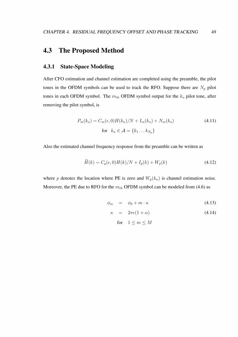
CHAPTER 4. RESIDUAL FREQUENCY OFFSET AND PHASE TRACKING 49
4.3 The Proposed Method
4.3.1 State-Space Modeling
After CFO estimation and channel estimation are completed using the preamble, the pilot
tones in the OFDM symbols can be used to track the RFO. Suppose there are Np pilot
tones in each OFDM symbol. The mth OFDM symbol output for the kn pilot tone, after
removing the pilot symbol, is
Pm(kn) = Cm(ε, 0)H(kn)/N + Im(kn) + Nm(kn) (4.11)
for kn ∈ A = {k1 . . . kNp}
Also the estimated channel frequency response from the preamble can be written as
H(k) = Cp(ε, 0)H(k)/N + Ip(k) + Wp(k) (4.12)
where p denotes the location where PE is zero and Wp(kn) is channel estimation noise.
Moreover, the PE due to RFO for the mth OFDM symbol can be modeled from (4.6) as
φm = φ0 + m · κ (4.13)
κ = 2πε(1 + α) (4.14)
for 1 ≤ m ≤ M

CHAPTER 4. RESIDUAL FREQUENCY OFFSET AND PHASE TRACKING 50
0 5 10 15 20 250
0.5
1
1.5
2
2.5
OFDM symbol index
Comparison of Phase Error
Pha
se e
rror
(ra
d)Without Noise
ML
Figure 4.4: Comparison of phase error for ε = 0.01: ML
where M is the total number of OFDM symbols in one packet. Then the maximum likeli-
hood (ML) estimate of the PE, φm, can be derived as
tan(φm) =Im[PmH∗]
Re[PmH∗](4.15)
Pm = [Pm(k1)Pm(k2) . . . Pm(kNp)]
H = [H(k1)H(k2) . . . H(kNp)]
Fig. 4.4 shows an example plot of actual PE without noise and the corresponding ML
estimates with respect to the OFDM symbol index when ε = 0.01. Assuming |φm−φm| ¿1, the tangent can be approximated by its argument and the ICI can also be approximated as
a zero mean Gaussian random variable for sufficiently large N by the central limit theorem

CHAPTER 4. RESIDUAL FREQUENCY OFFSET AND PHASE TRACKING 51
[21]. The estimation error can be written then as
φm − φm ≈ Dm/Em
where Dm and Em are defined as
Dm ,( ∑
kn∈AIm[(NfN
(ε)H∗(kn) + (Nm(kn) + Im(kn))e−jφm)
·(f ∗N(ε)H∗(kn) + (Wp(kn) + Ip(kn))∗)])
Em ,( ∑
kn∈ARe[(NfN
(ε)H∗(kn) + (Nm(kn) + Im(kn))e−jφm)
·(f ∗N(ε)H∗(kn) + (Wp(kn) + Ip(kn))∗)])
At high SNR, the above equation can be further approximated by,
φm − φm ≈ D′m/E
′m
where D′m and E
′m are defined as
D′m ,
( ∑
kn∈AIm[(Nm(kn) + Im(kn))f ∗N(ε)H∗(kn)e−jφm
+fN(ε)H(kn)(Wp(kn) + Ip(kn))∗])
E′m ,
( ∑
kn∈A|fN(ε)H(kn)|2)
from which we can deduce that the estimate is conditionally unbiased
E[φm − φm|ε,H(kn)] = 0 (4.16)

CHAPTER 4. RESIDUAL FREQUENCY OFFSET AND PHASE TRACKING 52
Moreover, the conditional variance of the estimate is
σ2ML = Var(φm − φm|ε)
≈ 2(1− f 2N(ε)) + σ2
N + σ2W
2Np · f 2N(ε)
(4.17)
where σ2N = E[|N(k)|2] and σ2
W = E[|Wp(k)|2]. Note that σ2ML is a function of ε. It
is not obvious how to determine σ2ML since the statistical distribution of ε is usually un-
known. Therefore, in order to design the robust estimator, σ2ML should be set according to
the expected worst case value of εmax in the acquisition range. In addition, the unknown
constants, σ2N and σ2
W , can be estimated in advance using the auto-correlation output of
the CFO estimation during the preamble. Suppose |J(n)| is the absolute magnitude of the
auto-correlation output,
|J(n)| = |Wa−1∑i=0
r(n + i)r∗(n + i + Ns)|
≈Wa−1∑i=0
|q(n + i)|2 (4.18)
where Ns is the repeating period, Wa is the averaging length and q(n) = h(n) ∗ s(n). Due
to the repeating property of the preamble, the noise variances can be estimated as follows:
E[|q(n)|2] ≈ |J(n)|/Wa
E[|r(n)|2] ≈ (Wa−1∑i=0
|r(n + i)|2)/Wa
σ2N = N · (E[|r(n)|2]− E[|q(n)|2]) (4.19)
σ2W = β · σ2
N (4.20)
where β is a known constant which depends on the channel estimation method. Therefore
combining (4.13), (4.17), (4.19) and (4.20), we obtain the following state-space model for

CHAPTER 4. RESIDUAL FREQUENCY OFFSET AND PHASE TRACKING 53
xm = [φm, κ]T .
xm = Fm−1xm−1 (4.21)
ym = Gmxm + qm (4.22)
where Fm−1 =
1 1
0 1
, Gm =
(1 0
)and
E[|q|2] = σ2ML =
2(1− f 2N(εmax)) + σ2
N(1 + β)
2Np · f 2N(εmax)
4.3.2 The Kalman Filter
From the above state-space model, the consecutive vector xm|m−1 and xm|m, with error
covariance matrix P , are recursively estimated given the measurement history and current
measurement ym through the Kalman filter. Based on this basic state-space representation
for RFO, the conventional Kalman equations are calculated as follows :
• Prediction step is
xm|m−1 = Fm−1xm−1|m−1
Pm|m−1 = Fm−1Pm−1|m−1FTm−1
• Update step is
Km = Pm|m−1GTm[GmPm|m−1G
Tm + σ2
ML]−1
xm|m = xm|m−1 + Km[ym −Gmxm|m−1]
Pm|m = Pm|m−1 −KmGmPm|m−1

CHAPTER 4. RESIDUAL FREQUENCY OFFSET AND PHASE TRACKING 54
Thus far, we have formulated the Kalman equations for recursively estimating the state vec-
tor xm. All that needs to be done to complete the recursion is to determine how the recursion
should be initialized. Since the CFO estimate is unbiased, E[κ] = 2π(1 + α)E[ε] = 0 and
E[φ0] = E[−pκ] = 0 from (4.13). Also E[κ2] can be approximately obtained from the
error variance of the CFO estimation [21]. Therefore, the initial estimate and initial value
for the error covariance matrix can be determined as
P0|0 = E[x0xT0 ] = σ2
κ
p2 −p
−p 1
(4.23)
x0|0 = E[x0] = E
[ −pκ
κ
]=
0
0
(4.24)
To demonstrate the features of the Kalman filtering as opposed to ML method, Fig.
4.5 shows an example plot of phase errors with the different RFO tracking methods when
ε = 0.01. Note that the proposed method can significantly reduce RFO induced phase error.
It has better performance because it utilizes not only instantaneous phase measurement but
also history of the phase estimation.
4.3.3 Complexity Consideration
In order to measure the computational complexity of different estimation methods, we use
the number of floating-point operations (flops). The LS phase fitting generally requires
O(M3) flops to obtain parameters where M is the number of samples used for the line
fitting. In contrast, the Kalman filter in the proposed method requires fewer than 100 flops
for each step and the complexity increases linearly with respect to M . Therefore, if more
than ten ML estimates are used for the LS phase fitting, the complexity of the proposed
method is lower than that of the LS phase fitting while achieving better performance. The
Kalman filter is usually of high complexity. But for our particular application, that uses
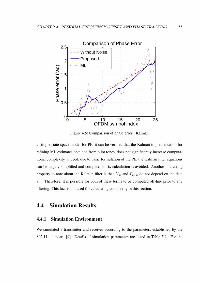
CHAPTER 4. RESIDUAL FREQUENCY OFFSET AND PHASE TRACKING 55
0 5 10 15 20 250
0.5
1
1.5
2
2.5
OFDM symbol index
Pha
se e
rror
(ra
d)
Comparison of Phase Error
Without Noise
Proposed
ML
Figure 4.5: Comparison of phase error : Kalman
a simple state-space model for PE, it can be verified that the Kalman implementation for
refining ML estimates obtained from pilot tones, does not significantly increase computa-
tional complexity. Indeed, due to basic formulation of the PE, the Kalman filter equations
can be largely simplified and complex matrix calculation is avoided. Another interesting
property to note about the Kalman filter is that Km and Pm|m do not depend on the data
xm. Therefore, it is possible for both of these terms to be computed off-line prior to any
filtering. This fact is not used for calculating complexity in this section.
4.4 Simulation Results
4.4.1 Simulation Environment
We simulated a transmitter and receiver according to the parameters established by the
802.11a standard [9]. Details of simulation parameters are listed in Table 5.1. For the

CHAPTER 4. RESIDUAL FREQUENCY OFFSET AND PHASE TRACKING 56
Table 4.1: Simulation ParametersSampling time, Ts 50nsFFT length, N 64Number of used subcarriers, Nu 52Number of pilot subcarriers, Np 4Guard interval length, Ng 16Subcarrier spacing 312.5 KHzModulation 4-QAM, 64-QAMPacket length 100 symbolsNumber of packets 10000Channel coding rate 1/2
channel model, only small-scale fading is considered. Both the distance dependent path
loss and the shadowing are assumed to be constant over the simulation and incorporated
into the SNR. The power delay profile for typical office environment, based on the ETSI
model A in Fig.2.2 [4], is generated and time variation model in Chap 2 is employed.
Details of random channel generations are described in Sec 3.4. Moreover, one packet is
composed of 100 OFDM symbols. The proposed timing synchronization method in Chap
3 and LS channel estimation are used and SNR estimation is carried out as stated in (4.19).
In order to clearly demonstrate the performance of the proposed method, RFO, ε, is set at
constant 0.1(= 31.25KHz) for 4-QAM modulation and 0.05(= 15.62KHz) for 64-QAM
modulation before initial CFO estimation.
4.4.2 Performance result
In Fig.4.6 and Fig.4.7, we present average PER of the proposed method for the different
values of SNR with no channel estimation error. Cases are also shown for the ideal per-
formance when ε is zero, for the performance with ML method using Np(=4) pilots as
specified in the standard, for the performance without RFO compensation. We see that the
proposed method is superior to the conventional method. In particular, the performance for

CHAPTER 4. RESIDUAL FREQUENCY OFFSET AND PHASE TRACKING 57
64-QAM modulation with higher SNR is greatly improved. The difference in the perfor-
mance with respect to SNR is expected from Fig.4.1. While the performance gain in the
low SNR region is mainly due to decreased PE estimation error, the performance gain at
high SNR mostly comes from ICI reduction by RFO compensation.
Fig.4.8 and Fig.4.9 show average PER performance of the proposed method with chan-
nel estimation error. It can be seen that the gap between the proposed method and ”Ideal”
is slightly increased. This effect occurs because the channel estimation error may make the
ML estimate of PE biased and this can cause the PE output of the Kalman filter to converge
to an incorrect estimate. Also, since it takes a few OFDM symbols for the Kalman filter to
correctly estimate the RFO, ICI is not completely compensated during the initial tracking
period. However, These factors induce almost negligible PER performance degradation
and the performance gain over ML method is even increased since the proposed method is
able to update channel estimation result using the estimated RFO.
Fig.4.10 shows the RFO estimation error variance of the proposed method with channel
estimation error when ε = 0.1. The variance is calculated using the RFO estimates from
the 10th, 50th and the last OFDM symbol in each packet. It can be seen in Fig.4.10 that
the the estimation performance improves as the OFDM symbol index increases since more
measurement history is used for the estimation. For SNR greater than 15dB, the proposed
method can reduce the error variance below 10−8 for the last OFDM symbol in the packet.
The resulting standard deviation of the RFO estimation error is less than 31.25Hz.
4.5 Conclusions
In this chapter, we propose a residual frequency offset (RFO) compensator that compen-
sates both RFO and RFO induced phase error (PE) by using a Kalman filter. In our pro-
posed method, after the state-space model for RFO and PE is derived, a Kalman filter is
applied to track and estimate RFO and PE simultaneously. This method, when compared

CHAPTER 4. RESIDUAL FREQUENCY OFFSET AND PHASE TRACKING 58
4 6 8 10 12 14 1610
−2
10−1
100
Average SNR (dB)
Ave
rage
PE
R
ProposedIdealMLWithout Comp
Figure 4.6: Average packet error rate for 4-QAM without channel estimation error (ε = 0.1)
16 18 20 22 24 26 2810
−2
10−1
100
Average SNR (dB)
Ave
rage
PE
R
ProposedIdealMLWithout Comp
Figure 4.7: Average packet error rate for 64-QAM without channel estimation error (ε =0.05)

CHAPTER 4. RESIDUAL FREQUENCY OFFSET AND PHASE TRACKING 59
4 6 8 10 12 14 1610
−2
10−1
100
Average SNR (dB)
Ave
rage
PE
R
ProposedIdealMLWithout Comp
Figure 4.8: Average packet error rate for 4-QAM (ε = 0.1)
16 18 20 22 24 26 2810
−2
10−1
100
Average SNR (dB)
Ave
rage
PE
R
ProposedIdealMLWithout Comp
Figure 4.9: Average packet error rate for 64-QAM (ε = 0.05)

CHAPTER 4. RESIDUAL FREQUENCY OFFSET AND PHASE TRACKING 60
0 5 10 15 20 2510
−9
10−8
10−7
10−6
10−5
10−4
Average SNR (dB)
Err
or v
aria
nce
100th
symbol50
th symbol
10th
symbol
Figure 4.10: Error variance of RFO estimation (ε = 0.1)
with LS phase fitting, offers improved estimation and tracking behavior for RFO with less
complexity. Numerical results show that the proposed method significantly overcomes the
performance degradation due to RFO and almost achieves ideal PER performance.

Chapter 5
Enhanced DFT-Based MMSE Channel
Estimation
In practical OFDM systems, in order to limit the interference to adjacent channels, some
subcarriers are set to zero. These non-existent subcarriers are are often referred to as
virtual carriers (VCs). Due to these VCs, conventional DFT-based approaches are not
directly applicable because they induce spectral leakage, which results in an error floor
for the mean square error (MSE) performance. To circumvent this problem, we propose
an enhanced DFT-based minimum mean square error (MMSE) channel estimator using a
Kalman smoother. Our approach is based on building a robust state-space model for chan-
nel frequency response (CFR) followed by Kalman filtering and smoothing to minimize the
effects of leakage. Time domain MMSE weighting is also used to suppress channel noise.
Our simulation results show that the proposed method almost achieves the performance of
the optimal MMSE estimator while having a limited computational complexity.
61

CHAPTER 5. ENHANCED DFT-BASED MMSE CHANNEL ESTIMATION 62
5.1 Introduction
OFDM is an effective technique for overcoming multipath fading and achieving high-bit-
rate transmission over wireless channels. However, without channel estimation, OFDM
systems have to use differential phase shift keying (DPSK), which has 3dB SNR loss com-
pared to coherent demodulation. If coherent OFDM is adopted, channel estimation be-
comes a necessary requirement and pilot tones are usually used for channel estimation. In
general, the realization of pilot-aided channel estimation is based on least square (LS) [31]
or minimum mean square error (MMSE) [30]. The LS approach is simple but has poor per-
formance, whereas the MMSE approach has good performance but is complex and requires
a priori knowledge of channel statistics. As a compromise between LS and MMSE, a dis-
crete Fourier transform (DFT) based channel estimation that utilizes the channel impulse
response has been widely studied for OFDM systems [31] [32].
Fig. 5.1 shows a block diagram of DFT-based channel estimation. This method trans-
forms the channel from the frequency domain into the time domain by an inverse discrete
Fourier transform (IDFT). After that, a time domain windowing is applied to the channel
impulse response assuming the window length is longer than the maximum delay spread of
the channel. Finally, this method transforms the channel impulse response back to the fre-
quency domain by a DFT. Hence, the noise in the taps beyond the maximum delay spread
of the channel is filtered out in the time domain and this improves a performance. However,
this method assumes that all subcarriers of the OFDM signal are used for pilot transmis-
sion. Otherwise, after the IDFT operation, the power may spill over all the taps in the time
domain, and the noise filtering process becomes inapplicable. For example, in the WLAN
802.11a standard, in order to limit the interference to adjacent channels, subcarriers at the
band edge of the shaping filter are left unmodulated and set to zero. These unused subcar-
riers are called virtual carriers (VCs) and hence a direct application of DFT-based channel

CHAPTER 5. ENHANCED DFT-BASED MMSE CHANNEL ESTIMATION 63
estimation can not be used. Furthermore, the CFR at VCs can not be estimated by conven-
tional channel estimation approaches. Fig. 5.2 shows a CFR of the OFDM system where
11 subcarriers out of total 64 subcarriers are VCs. Although VCs are located at both edges
of the bandwidth, this figure shows the CFR from 0 to 64 instead of from -32 to 32 since
the DFT is periodic. It can be seen that direct application of a DFT to the CFR leads to
leakage in the time domain. In other words, windowing in the frequency domain can lead
to severe distortion in the time domain and hence the resulting channel estimate becomes
erroneous.
A windowed DFT-based channel estimation was proposed in [33] to reduce an aliasing
error and suppress the noise, but it requires searching for an optimal generalized Hanning
window shape to minimize MSE. Furthermore, implementation complexity is too high to
be used in practical systems for the non-interpolation case. In [34], robust Wiener filter-
ing is applied to eliminate the leakage effect due to absence of pilot symbols in the VCs.
This approach tried to improve BER performance by combining Wiener interpolation and
Wiener filtering for interpolation cases.
In this chapter, I present an enhanced DFT-based channel estimation method with sim-
ple Kalman filtering and smoothing. Moreover, a weighting function is applied to the
effective channel impulse response. The weighting function is chosen so that the MSE
between CFR and its estimate is minimized.
5.2 Kalman Smoothing
Autoregressive (AR) modeling is commonly used to model discrete time random processes.
This is due to the simplicity with which the parameters can be computed and due to their
correlation matching property. AR process of order p can be generated as

CHAPTER 5. ENHANCED DFT-BASED MMSE CHANNEL ESTIMATION 64
LS IFFT FFT
Freq domain Time domain Freq domain
H(1)
H(N)
H(2)
h(L)
H’(2)
H’(N)
H’(1)
0
h(1)
Figure 5.1: Block diagram of DFT-based method

CHAPTER 5. ENHANCED DFT-BASED MMSE CHANNEL ESTIMATION 65
0 20 40 600
0.5
1
1.5
2
index
mag
nitu
deIdealLS
Figure 5.2: Existence of virtual subcarriers
xn = −p∑
k=1
akxn−k + wn (5.1)
where w(n) is a complex white Gaussian noise process with uncorrelated real and imag-
inary components. Using Yule-Walker equations, the corresponding autocorrelation matrix
can be calculated using the autocorrelation function R as [35],
Rxa = −v (5.2)

CHAPTER 5. ENHANCED DFT-BASED MMSE CHANNEL ESTIMATION 66
where
Rx =
R(0) R(−1) · · · R(−p + 1)
R(1) R(0) · · · R(−p + 2)...
... . . . ...
R(p− 1) R(p− 2) · · · R(0)
a =(
a1 a2 · · · ap
)T
v =(
R(1) R(2) · · · R(p))T
For a non-interpolation channel estimation case, increasing the order of the AR model
not only increases computational complexity but also degrades the estimation performance
due to singularity of the channel correlation matrix, Rx, [36]. Suppose the LS estimate of
the channel frequency response is Hk and the channel dynamics follows an AR(1) model,
then a state space model for the CFR can be written as
Hk = A ·Hk−1 + qk−1
Hk = Hk + rk
where Hk is the CFR at index k, qk−1 ∼ N(0, Qk−1) and rk ∼ N(0, Rk). Using the
above equations, the prediction and update steps of the Kalman filter are :

CHAPTER 5. ENHANCED DFT-BASED MMSE CHANNEL ESTIMATION 67
Prediction steps :
mp = A ·mk−1
Pp = A · Pk−1 · AH + Qk−1
Update steps :
Kk = Pp · (Pp + Rk)−1
mk = mp + Kk(Hk −mp)
Pk = Pp −KkPp
A can be obtained simply as the ratio of correlations of Hk as A ≈ R(1)/R(0) from the
Yule-Walker method. Also, Qk−1 ≈ R(0) − |R(1)|2/R(0). The two unknown correlation
values, R(1) and R(0), can be estimated from an LS estimate of the channel frequency
response. In practice, the Kalman filter equations easily cope with missing values or VCs.
When missing values occur, the prediction steps are processed as usual, the update steps
are changed as mk = mp and Pk = Pp. After obtaining the Kalman filter output, then the
Kalman smoother is applied to the Kalman filtered output. The Kalman smoother calculates
recursively the state posterior distributions.
p(Hk|H0:N−1) = N(Hk|msk, P
sk ) (5.3)
The difference between filtering and smoothing is that the smoothed outputs are con-
ditioned to all of the measurement data, while the filtered outputs are conditioned only to
the measurement obtained before and at the time step k. So the smoothed output can be
calculated from the Kalman filter result by recursions as follows:

CHAPTER 5. ENHANCED DFT-BASED MMSE CHANNEL ESTIMATION 68
0 20 40 600
0.5
1
1.5
2
index
mag
nitu
deIdealFilterFilter+Smooth
Figure 5.3: Kalman filtering and smoothing output, SNR=10dB
P−k+1 = APkA
H + Qk
Ck = PkAH(P−
k+1)−1
msk = mk + Ck(m
sk+1 − Amk)
P sk = Pk + Ck(P
sk+1 − P−
k+1)CHk
starting from the last step N−1, with msN−1 = mN−1 and P s
N−1 = PN−1. Fig.5.3 shows
an example plot of output of Kalman filtering and smoothing at SNR=10dB when missing
values occur between k = 27 and k = 37. It can be seen that smoothing significantly
decreases the estimation error of filtering above.

CHAPTER 5. ENHANCED DFT-BASED MMSE CHANNEL ESTIMATION 69
5.3 MMSE Filtering in the time domain
By the IDFT operation, we transform the entire channel estimate obtained from the Kalman
prediction into a time domain channel impulse response
hkal(n) =1
N
N−1∑
k=0
msk exp(j2πkn/N) (5.4)
Since the prediction steps change white noise into colored Gaussian noise, the resulting
correlation vector of the colored noise in the time domain can be obtained by the scaled
IDFT of P sk
rnn(m) = E[nl+mn∗l ] =1
N2
N−1∑
k=0
P sk exp(j2πkm/N) (5.5)
The MMSE filtering matrix, M , in the time domain can be derived from the following
equations,
min|h−M · hkal(n)|2 (5.6)
By the orthogonality principle, M can be written as
M = Rhh · (Rhh + Rnn)−1 (5.7)
where
Rnn = t(rnn)
Rhh = E[hhH ]

CHAPTER 5. ENHANCED DFT-BASED MMSE CHANNEL ESTIMATION 70
where t denotes an operator that transforms a vector into a Toeplitz matrix. Since the
time domain correlation matrix of the channel impulse response is usually unavailable, Rhh
for a uniform channel power delay profile is used instead for robustness of the estimator.
Assuming a WSSUS (wide sense stationary uncorrelated scattering) channel [37], Rhh is
given by
Rhh =
1N
R(0) 0
0 0
(5.8)
R(0) = E[HkH∗k ] =
N−1∑n=0
|h(n)|2 (5.9)
where NGI denotes the length of the cyclic prefix and I represents a NGI by NGI iden-
tity matrix. Since the number of virtual carriers at the left and right side for the guard band
are the same, the resulting Rnn is a real matrix. Therefore, the resulting M matrix is a
real NGI by N matrix. Based on the above analysis, the overall estimation step can be
summarized as
msk = S(HLS) (5.10)
Htotal = F ·M ·G ·msk (5.11)
where S denotes a Kalman smoother, HLS is an initial LS estimate of the channel
frequency response, G is an N by N IDFT matrix and F is an N by NGI DFT matrix.

CHAPTER 5. ENHANCED DFT-BASED MMSE CHANNEL ESTIMATION 71
5.4 Complexity issues
In order to measure the computational complexity of different estimation methods, we use
the number of complex multiplications. The MMSE estimation generally requires O(N2)
and the window method [33] requires Nu + N + (2N/3)log2N + Nu. In contrast, for the
proposed method, a Kalman smoother requires O(N) and MMSE filtering requires NGI ·N .
So the total required complex multiplication is O(N)+N ·NGI +(2N/3)log2N . Although
the proposed method may appear to increases computational complexity over the window
method, the window method is very sensitive to window size which needs to be decided by
a complex optimization procedure. Therefore, implementation complexity of the window
method is much higher than that of the proposed method. To summarize, the proposed
method requires much less computational complexity than MMSE, while achieving almost
equivalent performance and it can be implemented simpler than the window method even if
it increases computational complexity a little in some sense. Note that although the Kalman
equations are usually of high complexity, for our particular application that uses a simple
state-space model for estimation, it can be verified that the Kalman implementation does
not significantly increase computational complexity and has better performance than the
window method. Furthermore, an interesting and useful property of the Kalman imple-
mentation is that, since the Kalman gain and error covariance matrix do not depend on the
data, it is possible for these terms to be calculated off-line prior to any filtering.
5.5 Simulation Results
5.5.1 Simulation Environment
We simulated a transmitter and receiver according to the parameters established by the
802.11a standard [9]. The simulation parameters are listed in Table 5.1. For the channel
model, only small-scale fading is considered. Both the distance dependent path loss and

CHAPTER 5. ENHANCED DFT-BASED MMSE CHANNEL ESTIMATION 72
Table 5.1: Simulation ParametersSampling time, Ts 50nsFFT length, N 64Number of used subcarriers, Nu 52Number of pilot subcarriers, Np 4Guard interval length, Ng 16Subcarrier spacing 312.5 KHzModulation 64-QAMNumber of OFDM symbols 64Number of packets 10000Channel coding rate 1/2
the shadowing are assumed to be constant over the simulation and incorporated into the
SNR. The channel is assumed to be stationary and the power delay profiles for a typical
office environment, based on the ETSI model A and B in Fig.2.2 [4], are generated. The
maximum delay spreads for these channels are 50ns and 100ns respectively. Details of
random channel generations are described in Sec 3.4. Finally, the proposed synchronization
methods in Chap 3 and Chap 4 are employed.
5.5.2 Performance result
A packet error rate was used as a performance measure for Chap 3 and Chap 4. However,
we focus on a mean square error (MSE) and a symbol error rate (SER) here for better
comparison of the proposed method with the past results [33][34].
Fig. 5.4 shows MSE plot of various estimation methods. ”LS” denotes least-square
initial channel estimate and ”Direct FFT” denotes a conventional DFT-based method that
simply pads zeros at the end of the time domain LS estimate of the channel. ”Kalman”
denotes the proposed method and ”MMSE” denotes optimal MMSE channel estimation. It
can be seen that the proposed method achieves almost the same performance as the optimal
MMSE estimator. The performance gain comes from the prediction of the CFR in the guard
band and MMSE filtering in the time domain. On the other hand, it can be seen that the

CHAPTER 5. ENHANCED DFT-BASED MMSE CHANNEL ESTIMATION 73
0 10 20 30 4010
−5
10−4
10−3
10−2
10−1
100
Average SNR (dB)
MS
E
KalmanMMSELSDirect FFT
Figure 5.4: MSE comparison in Channel A
0 10 20 30 4010
−4
10−3
10−2
10−1
100
Average SNR (dB)
SE
R
KalmanMMSELSDirect FFT
Figure 5.5: SER comparison in Channel A

CHAPTER 5. ENHANCED DFT-BASED MMSE CHANNEL ESTIMATION 74
0 10 20 30 4010
−5
10−4
10−3
10−2
10−1
100
Average SNR (dB)
MS
E
KalmanMMSELSDirect FFT
Figure 5.6: MSE comparison in Channel B
conventional DFT-based method quickly reaches an error floor due to aliasing.
Average SER performance is presented in Fig.5.5. The proposed method experiences
negligible performance loss in terms of SER compared to optimal MMSE and achieves
more than 2dB gain over LS channel estimation. The performance gain becomes more
obvious in Channel B as shown in Fig. 5.6 and Fig. 5.7. It can be seen that the proposed
method actually achieves the same SER performance as optimal MMSE estimation. There
are two reasons for this. First, since we assumed a uniform PDP when we derive the
proposed estimator due to lack of channel statistics, Channel B looks more like a uniform
power distribution than Channel A. In other words, the model risk that comes from our
assumption can be decreased as the RMS delay spread increases. Moreover, larger RMS
delay spread leads to more frequency selectivity and hence leads to more variation in the
LS measurement data in the frequency domain. Therefore, AR modeling in the frequency
domain becomes more exact and better filtering and smoothing are possible.

CHAPTER 5. ENHANCED DFT-BASED MMSE CHANNEL ESTIMATION 75
0 10 20 30 4010
−4
10−3
10−2
10−1
100
Average SNR (dB)
SE
R
KalmanMMSELSDirect FFT
Figure 5.7: SER comparison in Channel B
5.6 Conclusions
In this chapter, I propose an enhanced DFT-based channel estimation using Kalman filter-
ing and smoothing for OFDM systems with VCs in a multipath fading channel. VCs are
used in OFDM systems to ease shaping filter implementation and to provide guard bands.
However, VCs cause dispersive distortion of a channel impulse response and prohibit the
use of conventional DFT-based channel estimation. The proposed method achieves almost
equivalent performance compared to optimal MMSE channel estimation. Furthermore, it
does not require a priori channel knowledge of statistics and the implementation complexity
is lower than complexity for optimal MMSE channel estimation.

Chapter 6
Throughput Enhancement for IEEE
802.11a Wireless LANs
Orthogonal frequency division multiplexing (OFDM) in combination with bit-interleaved
coded modulation (BICM) is an efficient and robust high-speed transmission technique
used in the IEEE 802.11a standard. In this chapter, using the request to send (RTS) /
clear to send (CTS) mechanism, we present a method to improve throughput performance
by adaptively changing constellation sizes and power distribution across the sub-carriers
without sacrificing throughput due to explicit feedback. Based on the theoretical analysis,
this complex maximization problem can be approximately solved by a simple iterative
algorithm. Simulation results show that the proposed method can significantly improve
throughput performance with low implementation complexity.
6.1 Introduction
Multi-carrier modulation (MCM) is a powerful and practical technique for high data rate
transmission over frequency-selective channels. Popular implementations of MCM include
orthogonal frequency division multiplexing (OFDM). IEEE 802.11a systems adopt OFDM
76

CHAPTER 6. THROUGHPUT ENHANCEMENT FOR IEEE 802.11A WIRELESS LANS77
in conjunction with coding and bit-interleaving, known as bit-interleaved coded modulation
(BICM). Conventional coded-OFDM systems, currently used in 802.11a systems, allocate
equal bits and power across the sub-channels. This uniform power distribution leads to
an inefficient use of power since the power loaded onto the sub-channels with deep fades
is most likely to be wasted. If channel information is available at the transmitter, then
the transmitter can allocate the bits and the power more efficiently. Indeed, over the past
decade, it has been shown that link adaptation can improve actual throughput performance
when knowledge of the channel is available at the transmitter.
Throughput is defined as the ratio of the average delivered data payload to the average
transmission time. It is the fundamental performance metric for reliable and efficient com-
munication accounting for all the overhead, inter-frame time and possible data retransmis-
sion time. There have been many link adaptation algorithms for throughput enhancement.
Automatic Rate Fallback (ARF) protocol [40] is used in the commercial WaveLAN- II net-
working devices. In this protocol, if two consecutive Acknowledgement frames (Ack) are
lost, the transmission rate is decreased and a timer is set. When either the timer expires or
the number of successfully received Ack reaches 10, the transmission rate is increased to
the higher rate and the timer is canceled. Although this scheme is easy to implement, this
scheme is purely heuristic and does not quickly react to channel variation.
A MAC Service Data Unit (MPDU)-based link adaptation scheme has been developed
in [41]. It is a table-driven approach and the basic idea is to pre-establish a best PHY
mode table by dynamic programming and the best PHY mode is indexed by the Signal to
Noise Ratio (SNR), MPDU size, and retransmission count. However, the suggested scheme
assumes the radio channel matches to a particular stochastic model and takes measured
SNR as the only input from the PHY layer. Therefore, it may not fully exploit the full
potential of PHY knowledge and can lead to sub-optimal results.
In [38] and [39], schemes which utilize full channel knowledge to minimize packet
error rate (PER) were presented. They can effectively increase throughput by adaptively

CHAPTER 6. THROUGHPUT ENHANCEMENT FOR IEEE 802.11A WIRELESS LANS78
assigning optimal power distribution across sub-carriers. However, since the number of
used sub-carriers are changing according to channel conditions, these schemes may result
in unavoidable spectral efficiency degradation.
In this chapter, we extend the scheme in [38] and present a throughput enhancement
method by deriving a simplified expression for the throughput in the 802.11a system. The
IEEE 802.11 MAC specifies for the contention-based distributed coordination function
(DCF) access method to exchange short control frames - RTS/CTS prior to data trans-
mission [9]. RTS/CTS handshaking is essentially a medium reservation scheme, and this
mechanism is one of the effective ways to alleviate the hidden node problem under the
DCF. Assuming channel reciprocity, we incorporate this mechanism for getting channel in-
formation at the transmitter without sacrificing throughput due to explicit feedback. After
acquiring channel knowledge, a simple iterative algorithm is used to select constellation
size and power distribution across the sub-carriers to enhance the throughput. Simulation
results show that the proposed method can significantly improve throughput performance.
However, the performance gain is dependent on channel estimation and synchronization
error, and an improved inner receiver is required to achieve the desired performance gain.
6.2 System Model
We consider an OFDM system having a fast Fourier transform (FFT) length N where a total
of Nu subcarriers are used for transmission. The transmitted signal s(n) is generated by
inverse fast Fourier transform (IFFT) of data symbols Ak and a guard interval, sometimes
known as a cyclic prefix, of length Tg = Ng · Ts is placed in front of the useful portion
Tu = N ·Ts of the signal to prevent inter-symbol interference (ISI). Ts denotes the sampling

CHAPTER 6. THROUGHPUT ENHANCEMENT FOR IEEE 802.11A WIRELESS LANS79
time period.
s(n) =1
N
Nu/2+1∑
k=−Nu/2
Ak · expj2πnk
N(6.1)
for −Ng ≤ n ≤ N − 1
The baseband impulse response of the channel is assumed to be in the form of
h(n) =L−1∑
l=0
h(l)δ(n− l) (6.2)
where L is the maximum delay spread of the channel and h(l) represent the complex gain
of the lth multi-path component assuming time invariance over one OFDM symbol. After
transmission over this multi-path channel, the samples at the receiver are
r(n) =L−1∑
l=0
s(n− l − nt) · h(l) · exp (j2πεn
N+ θ) + n(n) (6.3)
where n(n) is complex white Gaussian noise at time n, nt = δt/Ts is the timing offset, θ is
unknown phase and ε = NTs ·δf is the normalized carrier frequency offset. After correctly
removing the guard interval assuming perfect synchronization, the signal is demodulated
by FFT. The resulting output at the subcarrier k is
Yk = Hk · Ak + Nk (6.4)
for −Nu/2 ≤ k ≤ Nu/2 + 1

CHAPTER 6. THROUGHPUT ENHANCEMENT FOR IEEE 802.11A WIRELESS LANS80
Channel
EncoderInterleaver
Bit Allocation
& Mapper
Power
AllocationOFDM Mod
Channel
OFDMDemod
ChannelEstimator
DemapperDeinterleaverChannelDecoder
Data
Out
Feedback
Figure 6.1: Block diagram of the simulated BIC-OFDM system
We define average SNR in the time domain as
SNR , E[|r(n)− n(n)|2]E[|n(n)|2] (6.5)
=E[|Xk|2] · E[|Hk|2]
E[|Nk|2]N
Nu
(6.6)
In our proposed method, assuming channel reciprocity, a clear to send (CTS) or an Ack
packet is used to estimate channel information on each sub-carrier at the transmitter. The
transmitter adjusts constellation size, which is the same for all sub-carriers, and power level
of each sub-carrier for near optimal throughput based on the estimated channel information.
Note that there exists a time delay between the channel estimation and the actual data
transmission. However, the time delay is much smaller than the transmission duration for a
data frame and the resulting channel estimation error is negligible. Fig. 6.1 shows a block
diagram of the simulated BIC-OFDM system. Also we evaluate our method’s performance
through simulation for both an ideal case and a more realistic case with channel estimation
error and synchronization error.

CHAPTER 6. THROUGHPUT ENHANCEMENT FOR IEEE 802.11A WIRELESS LANS81
Table 6.1: IEEE 802.11a PHY parametersParameters Value CommentstSlotTime 9 µs slot timetSIFS 16 µs SIFS timeaCWmin 15 min contention window sizeaCWmax 1023 max contention window sizetPLCPPreamble 16 µs PLCP preamble durationtPLCPHeader 4 µs PLCP signal field durationtSymbol 4 µs OFDM symbol time
6.3 Throughput Enhancement
6.3.1 Throughput Analysis
The IEEE 802.11a standard specifies an optional four way hand-shaking procedure, known
as request to send (RTS) / clear to send (CTS) mechanism. Before transmitting a packet,
a station reserves the channel by sending a RTS short frame. The destination station ac-
knowledges the RTS frame by sending the CTS frame, and the normal packet transmission
and Ack response occurs afterwards. The RTS and CTS frames carry the information of
the length of the packet to be transmitted. This information can be read by any listening
stations. Therefore, by detecting either the RTS or CTS frames, the neighboring stations
can delay transmissions and thus avoid collisions. [42].
In this study, we assume no collision of a RTS frame. Timing diagrams of fragment
bursts in the RTS/CTS mechanism are shown in Fig. 6.2 and 6.3. We also assume all con-
trol frames and a Physical Layer Convergence Procedure (PLCP) header are successfully
transmitted since the probability of error in a data frame is much larger than that of other
frames. Table 6.1 lists the related characteristics for the IEEE 802.11a PHY [9].
From the Fig. 6.2 and 6.3, we notice that transmission cycle can be represented by two
time duration as follows: one time duration when a packet is successfully transmitted and
the other time duration when a packet is lost. These two time durations can be represented
CHAPTER 6. THROUGHPUT ENHANCEMENT FOR IEEE 802.11A WIRELESS LANS82
as Ts and Tf , which are defined in the following equations,
Ts = tData + tSIFS + tAck + SIFS
Tf = tData + AckTimeout + backoffi
+ tRTS + tSIFS + tCTS + tSIFS (6.7)
where Ts denotes the time duration when a packet is successfully transmitted, Tf denotes
the time duration when a packet is lost and AckTimeout is equal to a tSIFS plus tAck plus
tSlotTime.
The transmission duration for data frame (tData), RTS frame (tRTS), Ack frame (tAck)
and CTS frame (tCTS) are defined as follows,
tData = tPLCPPreamble + tPLCPHeader
+ d28 · 8 + (16 + 6) + L · 8c
e · tSymbol
tRTS = tPLCPPreamble + tPLCPHeader
+ d20 · 8 + 22
ce · tSymbol
tAck = tPLCPPreamble + tPLCPHeader
+ d14 · 8 + 22
ce · tSymbol
tCTS = tAck (6.8)
where L denotes a packet length in bytes and c denotes total data bits in one OFDM symbol.
The random backoff interval is in the unit of tSlotTime and this random integer is uni-
formly distributed over the interval [0,CW]. CW means a contention window size and
its initial value is aCWmin. In the case of unsuccessful transmission, CW is updated to
[2× (CW +1)− 1]. Once CW reaches aCWmax, it remains at that value until it is reset. In
the case of successful transmission, CW is reset to aCWmin. The average backoff interval

CHAPTER 6. THROUGHPUT ENHANCEMENT FOR IEEE 802.11A WIRELESS LANS83
RTS
CTS
Frame1
ACK ACK
Frame2
SIFS SIFS
SIFS SIFS
Figure 6.2: Timing of successful frame transmission
RTS
CTS
Frame1
ACK Timeout
CTS
RTS
SIFS
SIFS
Backoff
Figure 6.3: Timing of frame transmission failure
before the ıth transmission attempt can be represented by [41]
backoffi =min[2i−1 · (aCWmin + 1)− 1, aCWmax]
2 / tSlotTime(6.9)
For a simple analysis, we assume only two stations are communicating with each other
with no interference. Under this assumption, the channel is always acquired after random
backoff.
From the above transmission cycle analysis, we can derive a throughput equation. Let
packet error rate (PER) be pe, then the throughput maximization problem can be written as
max8L∑∞
k=0(1− pe) · pke · (kTf + Ts)
(6.10)
where k denotes retransmission attempts. Since Ts and Tf are not dependent on power
distribution and they are constants for given c, optimal power distribution for (6.10) can be
approximately obtained by solving the minimum PER problem.

CHAPTER 6. THROUGHPUT ENHANCEMENT FOR IEEE 802.11A WIRELESS LANS84
6.3.2 The Minimum PER Problem
Symbol error probability for square QAM modulation is given by [46]
ps ≤ 4 ·Q(√
3 · E[|Xi|2] · Pi · |Hi|2E[|Ni|2] · (2m − 1)
)(6.11)
where m is a constellation size in bits. Using the Chernoff bound, the average un-coded bit
error probability over the sub-carriers is
pave ≤ 2
m ·Nd
·Nd∑i=1
exp
(−1.5 · E[|Xi|2] · Pi · |Hi|2
E[|Ni|2] · (2m − 1)
)(6.12)
where Nd is the number of data sub-carriers. It was proved in [38] that minimizing PER is
equivalent to minimizing (6.12). Therefore, the minimum PER problem can be simplified
as
min log
[N∑
i=1
e−γi·Pi
]
s.t.∑
Pi = P, Pi ≥ 0 (6.13)
where γi = 1.5·E[|Xi|2]·|Hi|2E[|Ni|2]·(2m−1)
and P represent a total power constraint. Note that the objective
function is convex and has a unique minimum. It can be solved by a simple iterative algo-
rithm using the Lagrange theorem. By the KKT condition, the optimal power distribution
for the minimum PER satisfies following equations.
−γi · e−γi·Pi = KN∑
i=1
1
−γi
ln(−K
γi
) = P (6.14)
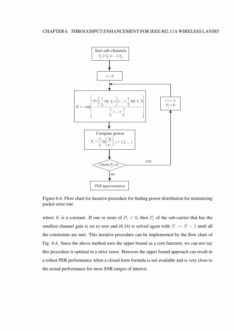
CHAPTER 6. THROUGHPUT ENHANCEMENT FOR IEEE 802.11A WIRELESS LANS85
i = N
Sort sub-channelsγ
1 > γ
2 > ... > γ
N
Compute power
PER approximation
i = i -1
Pi = 0
yes
no
γ
γ
γ
γ
γ γ( )
++
++
+
−=
i
i
i
P
K
��
��
��
1...
1
ln1
...)ln(1
exp
1
1
1
−
j = 1,2, ... iγ γ
=
jj
j
KP
��ln
1 −−
Check P < 0j −
Figure 6.4: Flow chart for iterative procedure for finding power distribution for minimizingpacket error rate
where K is a constant. If one or more of Pi < 0, then Pj of the sub-carrier that has the
smallest channel gain is set to zero and (6.14) is solved again with N → N − 1 until all
the constraints are met. This iterative procedure can be implemented by the flow chart of
Fig. 6.4. Since the above method uses the upper bound as a cost function, we can not say
this procedure is optimal in a strict sense. However the upper bound approach can result in
a robust PER performance when a closed form formula is not available and is very close to
the actual performance for most SNR ranges of interest.

CHAPTER 6. THROUGHPUT ENHANCEMENT FOR IEEE 802.11A WIRELESS LANS86
6.3.3 Throughput Enhancement Method
After acquiring the optimal power distribution for minimum PER, (6.12) can be calculated
again as
p∗ave ≤2
m ·N∗ ·N∗∑i=1
exp
(−1.5 · E[|Xi|2] · P ∗
i · |Hi|2E[|Ni|2] · (2m − 1)
)(6.15)
where N∗ is the number of sub-carriers used after the optimization procedure. It can be
shown that the probability of decoding the all-zero codeword as the ıth codeword with
distance d is upper bounded by [43].
pd ≤ [4 · p∗ave(1− p∗ave)]d/2 (6.16)
Using the above quantity, the union bound on the first-event error probability, p∗u, is bounded
by
pu ≤∞∑
d=dfree
ad · pd (6.17)
where ad is the total number of error events of distance d. From this union bound, the
resulting PER, p∗e, can be predicted heuristically using the method in [38] and [44].
pe ≈Lβ· pu
1 + Lβ· pu
(6.18)
where β is a constant which can be obtained by empirical fitting. Therefore, the constella-
tion size m for maximizing (6.10) can be obtained using the predicted PER. Fig. 6.5 shows
an example plot of constellation size selection during a 50ms interval. Diamond shapes in
the x-axis represent the times of erroneous packet receptions and the bottom plot represents
an average channel gain across sub-carriers at that time. It can be seen that the proposed

CHAPTER 6. THROUGHPUT ENHANCEMENT FOR IEEE 802.11A WIRELESS LANS87
method finds the best constellation size for maximum throughput even if it results in more
packet errors. In other words, the proposed method compensates the decreased spectral
efficiency due to the power optimization by assigning an optimal constellation size to max-
imize the throughput. Based on the results from our analysis, the throughput enhancement
method can be summarized by following steps:
1. Set the constellation size m for modulation.
2. Calculate Ts and Tf based on the constellation size and the number of retransmission
attempts at that time.
3. Find a power distribution for minimum PER.
4. Calculate throughput using PER, Ts and Tf obtained from step (3) and (2). (6.3.1)
5. Change constellation size and go back to step (2) until all throughput values for all
possible constellation sizes are obtained.
6. Find the maximum among the obtained throughput values and set constellation size
and power distribution according to the maximum.
6.4 Simulation Results
6.4.1 Simulation Environment
To evaluate the performance of the proposed method in frequency selective channels, a
simulator has been developed according to the parameters specified in the 802.11a standard
[9]. We assume an infinite resolution for an analog to digital converter and a perfectly
linear amplifier at the transceiver. The simulation parameters are listed in Table 6.2. For
the channel model, only small-scale fading is considered. Both the distance dependent path

CHAPTER 6. THROUGHPUT ENHANCEMENT FOR IEEE 802.11A WIRELESS LANS88
0 0.01 0.02 0.03 0.04 0.050
2
4
6
m
Time (seconds)
0 0.01 0.02 0.03 0.04 0.050
1
2
3
Time (seconds)
E[|H
k|2
Packet error
Figure 6.5: An exemplary plot of constellation size variation with respect to time
loss and the shadowing are assumed to be constant over the simulation and incorporated
into the SNR. Two different power delay profiles (PDPs), Channel A and B in Fig 2.2[4],
are generated and the time variation model in Chap 2 is employed. Details of random
channel generations are described in Sec 3.4. Moreover, packet length, L, is set to be
540 bytes and the proposed synchronization methods in Chapter 3 and 4 and the proposed
channel estimation method in Chapter 5 are used for simulation.
6.4.2 Performance of the Proposed Inner Receiver
Fig. 6.6 and Fig. 6.7 show the comparison of performance between a conventional 802.11a
system and the system with the proposed synchronization and channel estimation methods
at the receiver in Channel A and Channel B. The ordinate represents throughput in Mbps
and the abscissa represents an average SNR defined in (6.5). It can be seen that the system
with the proposed methods significantly improves throughput over a conventional 802.11a

CHAPTER 6. THROUGHPUT ENHANCEMENT FOR IEEE 802.11A WIRELESS LANS89
Table 6.2: Simulation ParametersSampling time, Ts 50nsFFT length, N 64Number of used sub-carriers, Nu 52Number of data sub-carriers, Nd 48Number of pilot sub-carriers, Np 4Guard interval length, Ng 16Subcarrier spacing 312.5 KHzModulation 4-QAM, 16-QAM, 64-QAMNumber of packets 10000Channel coding rate 1/2Packet length 540 Bytes
system in all SNR region we have tested. The performance gain for Channel B is much
larger than that for Channel A. Furthermore, the performance gain increases as the mod-
ulation becomes more complex. As shown in Chapter 3, this result is expected since a
conventional timing estimator often does not find a good timing boundary for the power
delay profile of Channel B. Hence, significant ISI and inter-carrier interference (ICI) are
induced. Moreover, as the constellation size increases, the system becomes more sensitive
not only to the synchronization error but also to the channel estimation error and an error
floor results.
6.4.3 Performance of Throughput Optimization
Fig. 6.8 shows the performance improvement by the throughput optimization. The solid
lines represent the performance of the system with the proposed inner receiver and without
an optimization. The line with circle represents the performance of the system with the
proposed optimization method and the proposed inner receiver. The ordinate represents
throughput in Mbps and the abscissa represents an average SNR defined in (6.5). We can
see that the proposed method improves throughput particulary for transition region between
two different modulations. The performance gain is maximized around the SNR boundary

CHAPTER 6. THROUGHPUT ENHANCEMENT FOR IEEE 802.11A WIRELESS LANS90
10 15 20 25 300
5
10
15
20
Average SNR (dB)
Thr
ough
put (
Mbp
s)
4−QAM16−QAM64−QAM
(a) Inner Rcv in Channel A
10 15 20 25 300
5
10
15
20
Average SNR (dB)
Thr
ough
put (
Mbp
s)
4−QAM16−QAM64−QAM
(b) Inner Rcv in Channel B
Figure 6.6: Throughput comparison for improved inner receiver: Channel A & B

CHAPTER 6. THROUGHPUT ENHANCEMENT FOR IEEE 802.11A WIRELESS LANS91
10 15 20 25 300
5
10
15
20
Average SNR (dB)
Thr
ough
put (
Mbp
s)
4−QAM16−QAM64−QAM
(a) Conventional system in Channel A
10 15 20 25 300
5
10
15
20
Average SNR (dB)
Thr
ough
put (
Mbp
s)
4−QAM16−QAM64−QAM
(b) Conventional system in Channel B
Figure 6.7: Throughput comparison for conventional system : Channel A & B

CHAPTER 6. THROUGHPUT ENHANCEMENT FOR IEEE 802.11A WIRELESS LANS92
of two different modulations, such as 16dB and 24dB, since the proposed method has more
degrees of freedom to select power allocation and constellation size. If SNR is larger than
30dB, the performance gain becomes negligible since the average SNR is large enough
to use 64-QAM modulation for all sub-carriers in this region. Note that the performance
improvement generally becomes larger as the frequency diversity increases. For example,
the performance improvement for Channel B is greater than that for Channel A as shown
in Fig. 6.8 and Fig. 6.9. This happens since less power is allocated to the sub-carriers with
low channel gains to increase the minimum distance of the channel code. Fig. 6.9 shows
the same throughput results with a conventional 802.11a system for comparison. We can
see that the system with the proposed methods significantly outperforms a conventional
system.
6.4.4 Benefits of Throughput Optimization
Fig. 6.10 shows the performance result of the throughput optimization with a conventional
receiver. Unlike the previous result, the improvement from the optimization is limited to
a small range of SNR for Channel A. Moreover, the optimization can degrade the system
performance in Channel B. The rationale behind this is that the channel estimation and
the synchronization error not only result in erroneous optimization at the transmitter but
also they degrade the system performance at the receiver. Therefore, the proposed opti-
mization method is more sensitive to the channel estimation and the synchronization error
than a conventional 802.11a system. The optimization consistently shows somewhat better
performance in Channel A where the channel estimation and the synchronization error are
smaller than Channel B.

CHAPTER 6. THROUGHPUT ENHANCEMENT FOR IEEE 802.11A WIRELESS LANS93
10 15 20 25 300
5
10
15
20
Average SNR (dB)
Thr
ough
put (
Mbp
s)
Opt+Inner
(a) adaptive transceiver with Inner Rcv in Channel A
10 15 20 25 300
5
10
15
20
Average SNR (dB)
Thr
ough
put (
Mbp
s)
Opt+Inner
(b) adaptive transceiver with Inner Rcv in Channel B
Figure 6.8: Throughput comparison for adaptive transceiver in Channel A & B
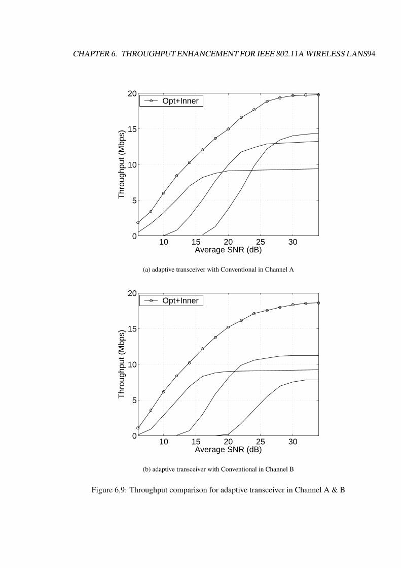
CHAPTER 6. THROUGHPUT ENHANCEMENT FOR IEEE 802.11A WIRELESS LANS94
10 15 20 25 300
5
10
15
20
Average SNR (dB)
Thr
ough
put (
Mbp
s)
Opt+Inner
(a) adaptive transceiver with Conventional in Channel A
10 15 20 25 300
5
10
15
20
Average SNR (dB)
Thr
ough
put (
Mbp
s)
Opt+Inner
(b) adaptive transceiver with Conventional in Channel B
Figure 6.9: Throughput comparison for adaptive transceiver in Channel A & B

CHAPTER 6. THROUGHPUT ENHANCEMENT FOR IEEE 802.11A WIRELESS LANS95
10 15 20 25 300
5
10
15
20
Average SNR (dB)
Thr
ough
put (
Mbp
s)
Opt only
(a) adaptive transceiver with Conventional in Channel A
10 15 20 25 300
5
10
15
20
Average SNR (dB)
Thr
ough
put (
Mbp
s)
Opt only
(b) adaptive transceiver with Conventional in Channel B
Figure 6.10: Throughput comparison for only adaptive transceiver in Channel A & B

CHAPTER 6. THROUGHPUT ENHANCEMENT FOR IEEE 802.11A WIRELESS LANS96
6.5 Conclusions
We propose a simple throughput enhancement method by deriving a throughput equation
for the 802.11a system. The key ideas are 1) RTS/CTS frame exchange is used to circum-
vent a hidden node problem and to acquire channel information at the transmitter before
the data transmission begins. an Ack frame is used to acquire channel information af-
ter successful data transmission and 2) the transmitter uses this information to optimize
throughput performance without reducing throughput due to explicit feedback. The com-
plexity of the optimum solution can be reduced by a simple iterative algorithm. A typical
office environment is simulated with system parameters specified in the 802.11a standard.
Our simulation results show that the proposed method can significantly improve through-
put performance. However, the performance gain depends on the channel estimation error
and the synchronization error. Therefore, an improved inner receiver is required to achieve
significantly improved performance. Finally, our method can be used to perform similar
analysis for other practical systems with different codings and other implementation con-
straints.

Chapter 7
Conclusion
7.1 Summary
In this section, each chapter of the thesis is briefly summarized. Chapter 2 describes charac-
teristics of small scale fading in wireless channels which are suitable for describing indoor
wireless communications. After a brief overview of the ETSI channel models, we propose a
closed form autocorrelation model for temporal variation of indoor wireless channels. It is
important to understand different characteristics and properties of indoor wireless channels
compared to those of the mobile wireless channels because the measurements for indoor
channels show distinct differences from the mobile channel measurements. The proposed
model gives rise to more peaky Doppler spectrum and has a wider spread of power spec-
trum than the Jakes’s model. Consequently, our proposed model can be used for more
accurate simulations of indoor wireless systems and we have shown that our model closely
matches indoor channel measurements.
In Chapter 3, we propose an adaptive timing estimation method for OFDM systems. By
changing an observation window length, the first arriving path can be located even though
it may not be the strongest path. By doing so, ISI and ICI can be effectively removed. Our
method does not require any prior knowledge, such as signal to noise ratio (SNR) or power
97

CHAPTER 7. CONCLUSION 98
delay profile, and is robust to various channel environments. In addition, it also provides an
estimate of instantaneous total received power and the maximum delay spread which can
then be used in other applications to increase system throughput. Our computer simulation
results show that the proposed method can significantly improve error rate performance.
The performance gain becomes higher as delay spread increases.
Chapter 4 describes a residual frequency offset (RFO) compensator that compensates
both RFO and RFO induced PE by using the Kalman filter. In our proposed method, after
the state-space model for RFO and PE is derived, a Kalman filter is applied to track and
to estimate RFO and PE simultaneously. This method, compared to least square (LS)
phase fitting, offers an improved estimation and tracking behavior for RFO and has less
complexity. Numerical results show that the proposed method significantly compensates
the performance degradation due to RFO and achieves an almost ideal PER performance.
In Chapter 5, we proposed an enhanced DFT-based channel estimation using Kalman
filtering and smoothing for OFDM systems with virtual subcarriers (VCs) in a multipath
fading channel. VCs are used to ease a shaping filter implementation and to provide a
guard band. However, it also causes dispersive distortion in a channel impulse response
and prohibits the use of conventional DFT-based channel estimation. Our proposed method
achieves almost equivalent performance compared to the optimal minimum mean square
error (MMSE) channel estimation. Furthermore, it does not require knowledge of channel
statistics, and the implementation complexity is lower than the optimal MMSE channel
estimation.
In Chapter 6, we propose a simple throughput enhancement method by deriving a
throughput equation for 802.11a systems. The key ideas are 1) ready to send (RTS)/clear
to send (CTS) frame exchange is used to circumvent a hidden node problem and to acquire

CHAPTER 7. CONCLUSION 99
channel information at the transmitter before the data transmission begins. An acknowl-
edgement (Ack) frame is used to acquire channel information after successful data trans-
mission begins and 2) the transmitter uses this information to optimize throughput perfor-
mance without reducing throughput due to explicit feedback. The complexity of the opti-
mum solution can be avoided by a simple iterative algorithm. A typical office environment
is simulated with system parameters specified in the 802.11a standard. Simulation results
show that the proposed method can significantly improve throughput performance. How-
ever, the performance gain is dependent on the channel estimation and the synchronization
error and hence an improved inner receiver is required to achieve improved performance.
7.2 Future Work
This thesis discusses a few interesting problems related to designing adaptive OFDM sys-
tems and provides some solutions to them. Still, many interesting theoretic questions are
open and many practical constraints should be considered for a practical implementation.
First, synchronization is one of the most critical issues in OFDM systems and other
communication systems. It has great impact on ther issues, such as channel estimation,
equalization and decoding, to be implemented in communication systems. In Chapter 3 and
Chapter 4, details of the proposed synchronization methods based on adaptive techniques
have been discussed. In wireless LAN (WLAN) systems, carrier frequency synchroniza-
tion and symbol synchronization are done using a preamble transmitted as the header of
the packet. Although our work did not assume that a user has access to statistical knowl-
edge of the channel, it is still based on an additive Gaussian noise assumption. Therefore,
the sensitivity of system performance under different assumptions should be studied to see
the robustness of our methods. In addition, this work is done at the expense of a reduced
bandwidth efficiency. Blind and/or semi-blind algorithms can improve the estimation ac-
curacy without pilots or training symbols. In this dissertation, we did not consider blind

CHAPTER 7. CONCLUSION 100
algorithms since they require significant statistical knowledge of both signals and channels
and can lead to a high computational complexity. Therefore, low computational complex-
ity blind algorithms should be studied to see if the performance of OFDM systems can be
further improved.
Second, only single-antenna wireless channel models are considered in this thesis.
However, new wireless networks have started to employ multiple antennas, which would
require more complex channel models. In addition, the distribution of channels for different
users may not be the same in these systems. Significant interference from inside or outside
of a single network can also exist. With more practical channel models, the mathematical
analysis of adaptive communications can become a daunting task. However, in principle,
the methods proposed in this thesis can be modified to be used in such practical channels
and could be verified by numerical simulations.
Third, the channel estimation method presented in Chapter 5 only considers a case for
indoor communication systems (WLAN). However, in a mobile channel, channel variation
within a OFDM packet can be significant and pilot subcarriers for channel estimation are
distributed across the time and the frequency. Consequently, interpolation techniques are
used to track the channel variation within a packet. Therefore, it would be interesting to
extend the result of this study to an mobile case such as a mobile worldwide interoperabil-
ity for microwave access (WiMAX). Further, a more sophisticated time series model can
be employed to represent a state-space model for a channel frequency response since an
autocorrelation matrix is no longer singular for an interpolation case. To derive a suitable
time series model, the Akaike’s information criterion or the Bayesian information criterion
can be used to determine the order of the time series model.
Finally, in Chapter 6, channel reciprocity is assumed to derive an optimal power alloca-
tion and a constellation size. In reality, however, the channel reciprocity is not perfect due
to the difference in hardware between a transmitter and a receiver. Therefore, the robust-
ness of the method to non-reciprocity should be investigated before applying it to practical

CHAPTER 7. CONCLUSION 101
communication systems. Furthermore, the only constraints we considered for the power
allocation is that it is greater than zero. However, there is a maximum allowed power
transmission for each subcarrier in real communication systems and hence the maximum
power constraint should be added in the objective function. For this case, there is no simple
iterative algorithm for optimization. This kind of problem can consequently increase imple-
mentation complexity significantly. Therefore, the benefits of the optimization should be
studied to see how much improvement can be achieved given the implementation complex-
ity. These analysis will lead to a better understanding of the adaptive OFDM transceiver
and to a more robust improvement of conventional OFDM systems without adaptation.

Bibliography
[1] R. V. Nee and R. Prasad, ”OFDM For Wireless Multimedia Communications”,
Artech House Publishers, 2000
[2] T. S. Rappaport, ”Wireless Communications: Principles and Practice”, Prentice
Hall, 2002.
[3] Donald C. Cox, ”Introduction to Wireless Communication”, EE276 Course
Reader, Stanford University, 2008
[4] J. Medbo and P. Schramm, Channel Models For HIPERLAN/2 in Different In-
door Scenarios, ETSI/BRAN document no. 3ERI085B
[5] S.J.Howard and K.Pahlavan, ”Doppler spread measurements of the indooor radio
channels”, Electron. letter., vol. 26, no. 2, pp. 107-109, Jan. 1990
[6] A. Domazetovic, L.J. Greenstein, N.B. Mandayam and I. Seskar, ”Estimating the
Doppler spectrum of a short-range fixed wireless channel”, IEEE Transactions
on Communications, vol. 53, No. 7, pp. 1123-1126, Jul. 2005
[7] S. Thoen, L. Van der Perre and M. Engels, ”Modeling the Channel Time-
Variance for Fixed Wireless Communications”, IEEE Communications Letters,
Vol. 6, No. 8, pp. 331-333, Aug. 2002.
102

BIBLIOGRAPHY 103
[8] Vinko Erceg. Zyray Wireless et al., ”TGn Channel Models”, IEEE 802.11-
03/940r4, May 2004.
[9] IEEE 802.11a-1999: Wireless LAN Medium Access Control (MAC) and Physical
Layer (PHY) Specifications: High Speed Physical Layer in the 5 GHz Band,
1999
[10] IEEE 802.16a-1999: IEEE Standard for Local and Metropolitan Area Networks
Part 16: Air Interface for fixed Broadband Wireless Access Systems, Amendment
2: Medium Access Control Modifications and additional Physical Layer Specifi-
cations for 2-11GHz, 2003
[11] Y. Mostofi and D. Cox, ”Mathematical Analysis of the Impact of Timing Syn-
chronization Errors on the Performance of an OFDM System”, IEEE Trans. on
Comm., vol. 54, no. 2, 2006
[12] J.Beek, M. Sandell and P. Borjesson, ”ML Estimation of Time and Frequency
Offset in OFDM Systems”, IEEE Trans. Signal Proc., vol.45, pp.1800-1805,
1997
[13] T. Schmidl and D. C. Cox, ”Robust frequency and timing synchronization for
OFDM”, IEEE Trans. Commun, vol.45, pp.1613-1621, 1997
[14] F. Classen, ”Systemkomponenten fur eine terrestrische digitale mobile Breitban-
dubertragung”, Ph.D Dissertation,the RWTH-Aschen Germany: Shaker Verlag,
1996
[15] M. Speth, F. Classen and H. Meyer, ”Frame synchronization of OFDM systems
in frequency selective fading channels”, Proc. Vehicular Tech. Conf., 1997
[16] K. Wang, M. Faulkner and I. Tolochko, ”Timing Synchronization for 802.11a
WLANs under Multipath Channels”, Proc. ATNAC 2003

BIBLIOGRAPHY 104
[17] S. Chang and B Kelly, ”Time synchronization for OFDM-based WLAN sys-
tems”, IEE Electronics Letters, vol.39, pp.1024-1026, 2003
[18] A. Fort, J. Weijers, V. Derudder, W Eberle and A. Bourdoux, ”A performance
and complexity comparison of auto-correlation and cross-correlation for OFDM
burst synchronization”, ICASSP Proceedings, Hong Kong, 2003
[19] S. Manusani, R. Kshetrimayum and R. Bhattacharjee, ”Robust Time and Fre-
quency Synchronization in OFDM based 802.11a WLAN systems”, Anual India
Conf., 2006
[20] A. Fort and W. Eberle, ”Synchronization and AGC proposal for IEEE 802.11 a
burst OFDM systems”, em IEEE Globe Comm., 2003
[21] P. Moose, ”A technique for orthogonal frequency division multiplexing fre-
quency offset correction”, IEEE Trans. Comm., vol. 42, pp.2908-2914, 1994
[22] J. Li, G. Liu and G. Giannakis, ”Carrier Frequency Offset Estimation for OFDM
based WLAN”, IEEE Signal Processing Letters, vol.8, pp.80-82, 2001
[23] S. Chang and E. Powers, ”Efficient frequency-offset estimation in OFDM-based
WLAN systems”, IEE Electronics Letters, vol.39, pp.1554-1555, 2003
[24] J. Lee, H. Lou and J. Cioffi, ”SNR Analysis of OFDM Systems in the Presence
of Carrier Frequency Offset for Fading Channels”, IEEE Trans. Wireless Comm.
vol.5, pp.3360-3364, 2006
[25] J. Jo, H. Kim and D. Han, ”Residual frequency offset compensation for IEEE
802.11a”, Vehicular Technology Conference, 2004
[26] J. Lee and S. Kim, ”Residual frequency offset compensation using the approxi-
mate SAGE algorithm for OFDM system”, IEEE Trans. Comm., vol.54, pp.765-
769, 2006

BIBLIOGRAPHY 105
[27] P. Chia-Sheng, W. Kuei-Ann, ”Synchronization for Carrier frequency Offset in
Wireless LAN 802.11a System”, Proc. Wireless Personal Multimedia Comms.
Conf., 2002
[28] B. Chen and C Tsai, ”Frequency offset estimation in an OFDM system”, IEEE
IEEE Third Workshop on Signal Processing Advances in, pp.150-153, 2001
[29] J. Liu and J. Li, ”Parameter estimation and error reduction for OFDM-based
WLANs”, IEEE Trans. Mobile Computing, vol.3, pp.152-163, 2004
[30] O. Edfors, M. Sandel, J.-J. van de Beek, S. K. Wilson and P. O. Borjesson,
”OFDM channel estimation by singular value decomposition”, IEEE Trans.
Commun., vol. 46, no. 7, pp. 931-939, Jul. 1998.
[31] J.-J. van de Beek, O. Edfors, M. Sandel, S. K. Wilson and P. O. Borjesson, ”On
channel estimation in OFDM systems”, Proc. IEEE VTC95, pp. 815-919, Jul.
1995.
[32] H.Minn and V.K. Bhargava, ”An Investigation into time-domain approach for
OFDM channel estimation”, IEEE Trans. Broadcasting, vol. 46, no. 4, pp. 240-
248, Dec. 2000
[33] B. Yang, Z. Cao and K. B. Letaief, ”Analysis of low-complexity windowed DFT-
based MMSE channel estimator for OFDM systems”, IEEE Tran. Commun., vol.
49, no. 11, pp. 1977-1987, Nov. 2001.
[34] Dong Li, Feng Guo, Guosong Li, Liyu Cai, ”Enhanced DFT Interpolation-based
Channel Estimation for OFDM Systems with Virtual Subcarriers”, Vehicular
Technology Conference, 1580-1584, Spring 2006/
[35] Marple SL Jr., ”Digital spectral analysis with applications”, Prentice Hall, New
Jersey, 1987/

BIBLIOGRAPHY 106
[36] Kareem E. Baddour and Norman C. Beaulieu, ”Autoregressive modeling for fad-
ing channel simulation”, IEEE Transactions on Wireless Communications 4(4):
1650-1662, 2005
[37] P. A. Bello. ”Characterization of randomly time-variant linear channels” IEEE
Trans., vol. CS-11, no. 4, pp 360-393, 1963
[38] O. Awoniyi, O. Oteri and F. Tobagi, ”Adaptive Power Loading in OFDM-based
WLANs and Resulting Performance Improvement in Voice and Data Applica-
tions”, Vehicular Technology Conference, vol.2, pp. 789-794, Fall 2005
[39] H. Moon, ”Efficient Power Allocation for coded OFDM Systems”, Ph. D. Dis-
sertation, Stanford University, 2004
[40] A. Kamerman and L. Monteban, ”WaveLAN-: A High-Performance wireless
LAN for the Unlicensed Band”, Bell Labs Technical J., pp.118-133, summer
1997
[41] D. Qiao, S. Choi and K. Shin, ”Goodput analysis and link adaptation for IEEE
802.11a wireless LANs”, IEEE Trans. Mobile Computing, vol.1, pp.278-292,
Oct 2002
[42] G. Bianchi, ”Performance analysis of the IEEE 802.11 distributed coordination
function”, IEEE Journal on Selected Areas in Communication, vol.18, no.3,
March 2000
[43] D. G. Wilson, ”Digital Modulation and Coding”, Prentice Hall 1996
[44] K. Rege and S. Nanda, ”Irreducible FER for Convolutional Codes with Random
Bit Puncturing: Application to CDMA Forward Channel”, Vehicular Technology
Conference, vol.2, pp.1336-1340, Spring 1996

BIBLIOGRAPHY 107
[45] W. C. Jakes, ”Microwave Mobile Communication”, Wiley Publishers, 1974
[46] A. Goldsmith, ”Wireless Communications”, Cambridge University Press, 2005