dissipation and kinetic physics of astrophysical plasma
TRANSCRIPT

Dissipation and Kinetic Physics of Astrophysical Plasma Turbulence
NSF PRAC project #1614664
Vadim RoytershteynSpace Science Institute
Blue Waters Symposium, Sunriver, OR, May 15-19, 2017
William Matthaeus University of DelawareJohn Podesta, Space Science InstituteStanislav Boldyrev, University of Wisconsin, MadsionAaron Roberts, NASA GoddardYuri Omelchenko, Space Science InstituteNikolai Pogorelov, University of Alabama, HuntsvilleGian Luca Delzanno, Los AlamosHoma Karimabadi, CureMetrix, IncHeli Hietala, UCLAWilliam Daughton, Los Alamos Hantao Ji, PrincetonJack Scudder, University of IowaSeth Dorfman, UCLA
Acknowledgements
Funding: NASA, NSF
Collaborators:
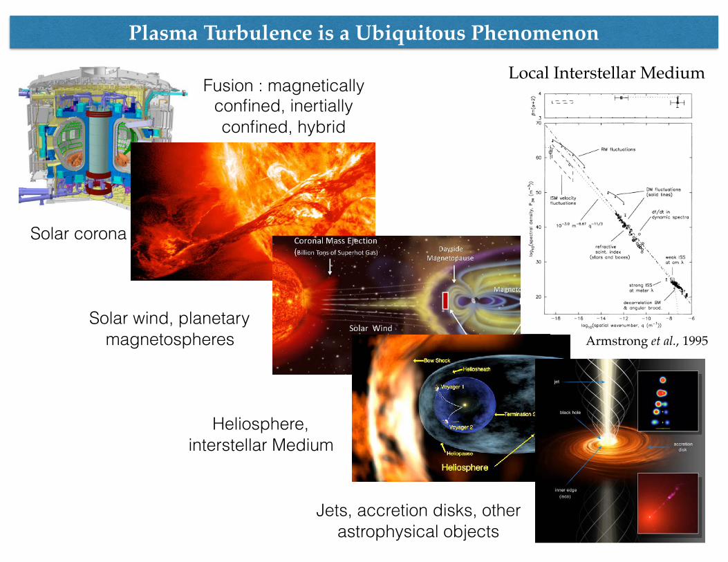
Plasma Turbulence is a Ubiquitous Phenomenon
90 million miles or ~ 100 Suns
Foundations of Black Hole Accretion Disk Theory 7
Figure 1: An artist’s rendition of a generic black hole accretion disk and jet. Inset figures include a timesequence of radio images from the jet in microquasar, GRS 1915+105 [204] and an optical image of the jetin quasar, M87 (Credit: J.A. Biretta et al., Hubble Heritage Team (STScI /AURA), NASA).
Living Reviews in Relativityhttp://www.livingreviews.org/lrr-2013-1
Fusion : magnetically confined, inertially confined, hybrid
Solar corona
Solar wind, planetary magnetospheres
Heliosphere, interstellar Medium
Jets, accretion disks, other astrophysical objects
Armstrong et al., 1995
Local Interstellar Medium

3
rsta.royalsocietypublishing.orgPhil.Trans.R.Soc.A373:20140155
.........................................................
10 −6 10−5 10−4 10−3 10−2 10−1 1 10
10−6
10−4
10−2
1
102
104
106
spacecraft frequency (Hz)
ACE MFI (58 days)ACE MFI (51 h)Cluster FGM + STAFF−SC (70 min)
−1.00 ± 0.04
−2.73 ± 0.01
−1.65 ± 0.01
tran
sitio
n re
gion
inertial range sub-ion rangef –1 range
trac
e po
wer
spe
ctra
l den
sity
(nT
2H
z–1)
lc ~ 106 km re ~ 1 km ri ~102 km
Figure 1. Typical trace power spectral density of the magnetic field fluctuations of a βi ∼ O(1) plasma in the ecliptic solarwind at 1 AU. Dashed lines indicate ordinary least-squares fits, with the corresponding spectral exponents and their fit errorsindicated. This spectrum represents an aggregate of intervals with each smaller interval being containedwithin the subsequentlarger interval—hence the higher frequencies of this spectrum are not representative of the interval describing the lowerfrequencies. At the largest scales is a 58 day interval [2007/01/01 00.00–2007/02/28 00.00 UT] from the MFI instrument onboard the ACE spacecraft, illustrating the large-scale forcing range (the so-called f−1 range). The inertial range is computedfrom a shorter 51 h interval [2007/01/29 21.00–2007/02/01 00.00 UT] also from the same instrument. Both these datasets are at1 Hz cadence, so they just begin to touch the beginning of the sub-ion range. The kinetic scale spectrum in the sub-ion scalerange is given by magnetometer data from the FGM and STAFF-SC instruments on the Cluster multi-spacecraft mission, fromspacecraft 4, while it was in the ambient solar wind [2007/01/30 00.10-01.10 UT] and operating in burst mode with a cadenceof 450 Hz—the two signals from both of these instruments have been merged as in [6]. The vertical dashed lines indicate thethree length scalesmentioned above:λc the correlation length,ρi the ion gyro-radius andρe the electron gyro-radius. (Onlineversion in colour.)
(a) Brief phenomenology of the energy cascadeWe ask the reader to turn their attention to figure 1, which shows a canonical power spectraldensity at 1 AU in the solar wind. We have chosen the power spectral density as it is not only thefocus of many, if not most, studies of turbulence, but also serves as a simple map to illustrate thescales of interest in the phenomena. It is also reflective—being the Fourier transform pair—of thetwo-point field correlation, another obsession of generations of turbulence researchers. Owing tothe extremely high speed of the solar wind, faster than most temporal dynamics in the system, wecan invoke the ‘Taylor frozen-in flow’ hypothesis to relate temporal scales to spatial scales (see [7]for caveats to this). Thus, although the abscissa shows a temporal scale of spacecraft frequency,for most of this spectrum (in the inertial range and above) it can be viewed as a proxy for spatialscales—some of which are marked at the top of the figure. In particular, we have highlighted fourdistinct regions of interest demarcated by three important length scales:
— The f −1 range. At these very small frequencies—corresponding to temporal scales overmany days—what we are actually measuring is the temporal variability of the source ofthe solar wind: the Sun and its solar atmosphere. Near the top of this range, we havethe first of our important length scales: the correlation length λc. Below this scale (higher
on February 27, 2017http://rsta.royalsocietypublishing.org/Downloaded from Focus of This Project: Turbulence in Solar Wind & Magnetosphere
• Turbulence is of interest because of:• Local energy input (e.g. to explain famously anomalous temperature profiles)• Transport of energetic particles (solar energetic particles, cosmic rays, etc)
• Solar Wind is the best accessible example of astrophysical (=large scale) plasma turbulence
Kiyani et al., 2015

The third panel of Fig. 1 shows the magnetic compressi-bility !B2
k=ð!B2k þ !B2
?Þ, which is enhanced to values of
$0:3 for compressive solar wind (T?=Tk > 1) with "k *1, as would be expected for the mirror instability. Thecompressibility becomes smaller for "k < 1, which isconsistent with the Alfven ion cyclotron mode; however,the power continues to be bounded by the mirror threshold.Linear mirror instability calculations [15] for T?=Tk > 1predict values of the magnetic compressibility between 0.8and 1; therefore, our measurements suggest a mixture ofwaves. Furthermore, it is interesting to note that the typicalvalue of the magnetic compressibility away from thethresholds is small $0:1. The existence of (compressive)magnetosonic or whistler branch waves at short wave-lengths [17] would seem to imply larger values of magneticcompressibility. If compressive waves are present, they arelikely to be highly mixed with Alfvenic fluctuations, so asto give a small average compressibility.
The bottom panel of Fig. 1 shows the average collisional‘‘age’’ in each ("k, T?=Tk) bin; the collisional age # isdefined as # ¼ $ppL=vsw, the Coulomb proton-proton col-lision frequency $pp multiplied by the transit time from theSun to 1 AU and is an estimate of the number of binarycollisions in each plasma parcel during transit from the Sunto the spacecraft. It is interesting, however obvious, that themore collisional plasma is more isotropic; away fromT?=Tk & 1, the plasma is relatively collisionless. It hasbeen shown recently [18] that collisional age organizessolar wind instabilities better than the traditional distinc-tion of ‘‘fast’’ and ‘‘slow’’ wind.
Figure 2 shows the magnetic fluctuations data j!Bjunnormalized by B. Linear instability thresholds associatewith the mirror, ion cyclotron (AIC), and oblique firehoseinstabilities [11] are overlaid. It is interesting to note that,as found by Hellinger et al. [11], the oblique firehose andthe mirror instabilities appear to constrain the observeddistribution of data, not the ion cyclotron nor parallel fire-hose instabilities (in spite of a larger growth rate); this maybe because both the mirror and oblique firehose are non-propagating instabilities. The regions of enhanced mag-netic fluctuations, near the mirror and oblique firehosethresholds, also correspond to measurements of enhancedproton temperature published elsewhere [19]. It is unclearif this indicates plasma heating due to anisotropy insta-bilities, in addition to pitch-angle scattering, or if the‘‘younger’’ (less collisional) plasma is merely hotter thanaverage.
Figure 3 shows histograms of the fluctuation amplitudesquared j!Bj2 in bins of collisional age; the white dotsshow the most probable value. The overall magnetic fluc-tuation power !B2 is a function of the collisional age, withthe magnetic power weaker by a factor of $100 for morecollisional plasma. This effect is a proxy for the tempera-ture anisotropy: collisional plasma is more isotropic and,therefore, further from the instability thresholds. This
underscores the important point that the power spectraldensity (PSD) of magnetic fluctuation power near 1 Hzin the solar wind is modified by these local instabilities.Previous studies of the PSD of short wavelength solar windturbulence have not accounted for this and should bereexamined [20–24]. If the j!Bj2 values in Fig. 3 aredivided by the measurement bandwidth (approximately5–10 Hz depending on sample rate), they can be comparedto power spectral density (PSD) measurements publishedpreviously (over the bandwidth of 0.3 to 11 Hz), noting thatthe power is dominated by the amplitude at the lowestfrequencies (0.3 Hz). A log-log fit to the most probable
mirrorAIC
FIG. 2 (color). The magnitude of magnetic fluctuations j!Bjaveraged into bins of T?=Tk vs "k. Enhanced power exists wellaway from the thresholds, as expected. The regions of enhanced!B corresponds to the enhanced proton heating in Liu et al.(2006).
FIG. 3 (color). Magnetic fluctuation amplitude j!Bj2 as afunction of the collisional age; the white dots are the most likelyvalue of j!Bj2 in each age bin. Magnetic fluctuations near theproton gyroradius (k% & 1=2) are suppressed in more collisionalplasma. Coulomb collisions maintain the isotropy of the protons,which then remain far from the instability thresholds. Note thatthis corresponds to a factor of 100 suppression of magneticpower !B2 over the full range of collisionality.
PRL 103, 211101 (2009) P HY S I CA L R EV I EW LE T T E R Sweek ending
20 NOVEMBER 2009
211101-3
15
Dynamic Alignment in MHD Turbulence
4/3~ λ
4/1~ λ2/1~ λl
Depletion of nonlinearity
line displacement:
Nonlinear interaction is reduced!θ
In our “eddy”, v and b are aligned within small angle . One can check that: θ
In our theory, this reduction of interaction is:
Energy spectrum is
λ
Alignment is scale-dependent
3
rsta.royalsocietypublishing.orgPhil.Trans.R.Soc.A373:20140155
.........................................................
10 −6 10−5 10−4 10−3 10−2 10−1 1 10
10−6
10−4
10−2
1
102
104
106
spacecraft frequency (Hz)
ACE MFI (58 days)ACE MFI (51 h)Cluster FGM + STAFF−SC (70 min)
−1.00 ± 0.04
−2.73 ± 0.01
−1.65 ± 0.01
tran
sitio
n re
gion
inertial range sub-ion rangef –1 range
trac
e po
wer
spe
ctra
l den
sity
(nT
2H
z–1)
lc ~ 106 km re ~ 1 km ri ~102 km
Figure 1. Typical trace power spectral density of the magnetic field fluctuations of a βi ∼ O(1) plasma in the ecliptic solarwind at 1 AU. Dashed lines indicate ordinary least-squares fits, with the corresponding spectral exponents and their fit errorsindicated. This spectrum represents an aggregate of intervals with each smaller interval being containedwithin the subsequentlarger interval—hence the higher frequencies of this spectrum are not representative of the interval describing the lowerfrequencies. At the largest scales is a 58 day interval [2007/01/01 00.00–2007/02/28 00.00 UT] from the MFI instrument onboard the ACE spacecraft, illustrating the large-scale forcing range (the so-called f−1 range). The inertial range is computedfrom a shorter 51 h interval [2007/01/29 21.00–2007/02/01 00.00 UT] also from the same instrument. Both these datasets are at1 Hz cadence, so they just begin to touch the beginning of the sub-ion range. The kinetic scale spectrum in the sub-ion scalerange is given by magnetometer data from the FGM and STAFF-SC instruments on the Cluster multi-spacecraft mission, fromspacecraft 4, while it was in the ambient solar wind [2007/01/30 00.10-01.10 UT] and operating in burst mode with a cadenceof 450 Hz—the two signals from both of these instruments have been merged as in [6]. The vertical dashed lines indicate thethree length scalesmentioned above:λc the correlation length,ρi the ion gyro-radius andρe the electron gyro-radius. (Onlineversion in colour.)
(a) Brief phenomenology of the energy cascadeWe ask the reader to turn their attention to figure 1, which shows a canonical power spectraldensity at 1 AU in the solar wind. We have chosen the power spectral density as it is not only thefocus of many, if not most, studies of turbulence, but also serves as a simple map to illustrate thescales of interest in the phenomena. It is also reflective—being the Fourier transform pair—of thetwo-point field correlation, another obsession of generations of turbulence researchers. Owing tothe extremely high speed of the solar wind, faster than most temporal dynamics in the system, wecan invoke the ‘Taylor frozen-in flow’ hypothesis to relate temporal scales to spatial scales (see [7]for caveats to this). Thus, although the abscissa shows a temporal scale of spacecraft frequency,for most of this spectrum (in the inertial range and above) it can be viewed as a proxy for spatialscales—some of which are marked at the top of the figure. In particular, we have highlighted fourdistinct regions of interest demarcated by three important length scales:
— The f −1 range. At these very small frequencies—corresponding to temporal scales overmany days—what we are actually measuring is the temporal variability of the source ofthe solar wind: the Sun and its solar atmosphere. Near the top of this range, we havethe first of our important length scales: the correlation length λc. Below this scale (higher
on February 27, 2017http://rsta.royalsocietypublishing.org/Downloaded from
“dispersion range” or “dissipation range”:
• internal kinetic scales are encountered, leading to partial onset of dissipation, but also to change in fluctuation properties;
• in weakly collisional plasma, dissipation is a collective effect
| z
Kinetic Effects in Plasma Turbulence (i.e. the Plasma Physics Aspects)
Cross-scale coupling in the inertial range via
• intense current sheets and reconnection
•ion temperature anisotropies•coupling between compressible and
incompressible fluctuations
Boldyrev, 2005Loureiro & Boldyrev, 2016Mallet et al., 2016
Bale et al., 2009
| z

A Variety of Models & Approximations Are Used to Tackle This Range of Scales
smaller scales
L: system size, energy injection scale,
correlation scaleion kinetic
scales
electron kinetic scales
debye lengthcollisional scale
(collisional)collisional
scale (c-less)
Magnetohydrodynamic approximation (MHD):
incompressible, fully compressible, kinetic MHD.. Hall MHD
multi-fluid multi-moments modelshybrid kinetic
…Landau FluidGyrokineticFully kinetic
…E +1
cv B = 0
@tv + v ·rv =1
cj B
@tB = crE rB =4
cjm
odel
com
plex
ity
In many situations, cross-scale coupling play a role an important role global dynamics. Full understanding of global evolution may require multi-scale, multi-physics models
@tfs + v ·rfs +qsms
E +
1
cv B
·rvfs = Cfs, fs0 , . . .
+ Maxwell’s equations
“First-Principle” description ofweakly coupled plasmas:
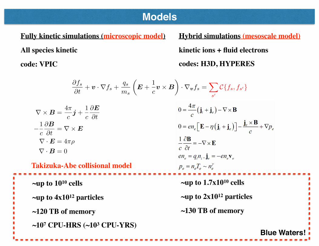
Models
@fs@t
+ v ·rfs +qsms
E +
1
cv B
·rvfs =
X
s0
Cfs, fs0
~up to 1010 cells
~up to 4x10¹² particles
~120 TB of memory
~107 CPU-HRS (~103 CPU-YRS)
Hybrid simulations (mesoscale model)
kinetic ions + fluid electrons
codes: H3D, HYPERES
Fully kinetic simulations (microscopic model)
All species kinetic
code: VPIC
rB =4
cj +
1
c
@E
@t
1
c
@B
@t= rE
r ·E = 4
r ·B = 0
~up to 1.7x10¹⁰ cells
~up to 2x10¹² particles
~130 TB of memory
Takizuka-Abe collisional model
Blue Waters!
p expensivesampling
efficientsampling
x
d
dtx = v
d
dtv = F /m
p
t=t1 x
p
t=t2x
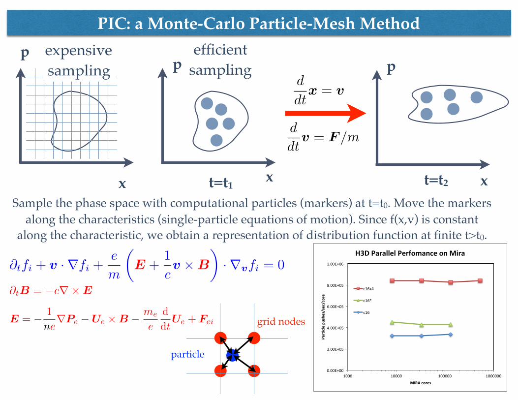
PIC: a Monte-Carlo Particle-Mesh Method
grid nodes
particle0.00E+00
2.00E+05
4.00E+05
6.00E+05
8.00E+05
1.00E+06
1000 10000 100000 1000000
Par$clepu
shes/sec/core
MIRAcores
H3DParallelPerfomanceonMira
c16x4
c16*
c16
Sample the phase space with computational particles (markers) at t=t0. Move the markers along the characteristics (single-particle equations of motion). Since f(x,v) is constant
along the characteristic, we obtain a representation of distribution function at finite t>t0.
@tB = crE
E = 1
nerPe Ue B me
e
d
dtUe + Fei
@tfi + v ·rfi +e
m
E +
1
cv B
·rvfi = 0

Problems Considered in Year 1
• Generation of intense current sheets at or above proton scales • Turbulence in low-β plasmas [in progress] • Universality of decay [in progress]
3D hybrid simulation of decaying turbulence3D hybrid simulation of solar wind-like turbulence
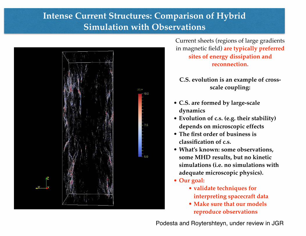
Intense Current Structures: Comparison of Hybrid Simulation with Observations
Podesta and Roytershteyn, under review in JGR
Current sheets (regions of large gradients in magnetic field) are typically preferred
sites of energy dissipation and reconnection.
C.S. evolution is an example of cross-scale coupling:
• C.S. are formed by large-scale dynamics
• Evolution of c.s. (e.g. their stability) depends on microscopic effects
• The first order of business is classification of c.s.
• What’s known: some observations, some MHD results, but no kinetic simulations (i.e. no simulations with adequate microscopic physics).
• Our goal: • validate techniques for
interpreting spacecraft data• Make sure that our models
reproduce observations

Example of Direct Comparison With Spacecraft Data: Properties of Intense Currents Sheets
X - 20 PODESTA AND ROYTERSHTEYN: ELECTRICAL CURRENTS IN THE SOLAR WIND
Table 1. Characteristics of 5s events in the simulation with L? = 128di
Property\Physical variable Jtrue JP dBx/dl dBy/dl dBz/dl
Mean (in units of B0/di) 0.204 0.103 0 0 0
Standard Deviation (B0/di) 0.122 0.0649 0.0822 0.0562 0.0697
Number of events 365 459 244 168 197
Mean separation distance (di) 381 299 563 814 697
Median separation distance (di) 214 203 377 544 366
Mean event size (di) 1.80 1.75 1.6 1.5 1.2
Mean peak value (B0/di) 0.949 0.508 0.489 0.330 0.403
Maximum peak value (B0/di) 1.68 0.922 0.864 0.761 0.584
Table 2. Characteristics of 5s events in the simulation with L? = 256di
Property\Physical variable Jtrue JP dBx/dl dBy/dl dBz/dl
Mean (in units of B0/di) 0.109 0.0746 0 0 0
Standard Deviation (B0/di) 0.0748 0.0479 0.0603 0.0416 0.0499
Number of events 2,881 4,249 2,522 1,349 2,033
Mean separation distance (di) 386 261 440 823 547
Median separation distance (di) 269 160 277 506 302
Mean event size (di) 2.83 1.95 1.7 1.8 1.3
Mean peak value (B0/di) 0.581 0.381 0.366 0.250 0.299
Maximum peak value (B0/di) 1.36 1.06 0.818 0.633 0.799
Table 3. Characteristics of 5s events in high speed solar wind data
Property\Physical variable Jtrue JP dBx/dl dBy/dl dBz/dl
Mean (pA/cm2) ? 0.0952 0 0 0
Standard Deviation (pA/cm2) ? 0.0725 0.0566 0.0698 0.0791
Number of events ? 1,336 660 977 879
Mean separation distance (di) ? 336 680 459 504
Median separation distance (di) ? 57.4 108 49.6 71.2
Mean event size (di) ? 3.2 3.1 2.8 3.1
Mean peak value (pA/cm2) ? 0.606 0.363 0.467 0.536
Maximum peak value (pA/cm2) ? 1.84 1.09 1.72 1.84
D R A F T February 22, 2017, 6:36am D R A F T
020406080100120
x
020
4060
80100
120
y
0
50
100
150
200
250
300
350
z
In many cases spacecraft data is 1D - a sample along spacecraft trajectory (with the exception
of multi-spacecraft missions, e.g. MMS, CLUSTER, THEMIS, etc)
Plasma data from the Wind 3DP instrument and magnetic field strength data from the Wind MFI instrument for
the two day interval (Podesta, 2017)
Sample periodic box along 1D trajectory to
model spacecraft data acquisition
Remarkable agreements between simulation and data
Helicities
0
0.2
0.4
0.6
0.8
1
0 100 200 300 400 500
2Hc(t)/E(t)
tΩci
HYPERS
H3D
H3D(b)
0
0.05
0.1
0.15
0.2
0 0.2 0.4 0.6 0.8 1
k minHm/E
2Hc/E
HYPERS
H3D
H3D(b)
H3D, initial condition A
HYPERS, I.C. B
H3D, I.C. B
TABLE III. System parameters for decay runs.
Run E”/-%
A 1.0 B 1.0 C 0.5 D 1.0
Initial value
2HJ.E
0.0 0.8 0.6 0.0
H,/E 4i”d
0.2 loo.0 0.0 100.0 0.2 100.0 0.0 loo.0
Value at tana,
E”/Eb 2HJE H,,,/E E
4.54x 10⁻³ - 3.17x 10-Z 0.992 1.36x lo-? 1.07 0.983 3.42x lo-* 1.88X 10-s 0.317 0.852 0.757 3.04x 10⁻² 0.945 0.2 7.16x IO-* 4.43 x 10-b
the evolution of the system. The initial H, = 0.0, so that dynamic alignment has negligible dynamical influence. In Fig. 4 a parametric plot in the 2H,/E, H,/E parameter is given. The ratio H,/E is seen to grow to near its maximum value of 1 prior to tana,, verifying the most obvious prediction of selective decay. The ratio 2HJE changes very little from its initial value, remaining far from its extremal values of & 1, indicating the absence of dynamic alignment. Figure 5 illustrates the evolution of various global quantities. The minimum energy principle discussed in Sec. II predicts a value of unity for 1 H,,, I/Eb, a consequence of condensation of Eb and H, into kmin, forming a long wavelength perfectly helical magnetic field. Figure 5 (a) illustrates the approach of run A to this helical state.
The dynamical evolution of the fractions of Eu and Eb residing in kmin is an indicator of the effectiveness of spectral back-transfer. The temporal behavior of these fractions, de- signated as E, (kmin j/E, and Eb (k,,, )/E,, are shown in Fig. 6. The ratio E, ( kmin )/ED stays roughly constant and small, but Eb (kmin )/Eb undergoes substantial increase. This implies that a substantial amount of Eb is accumulating in the large scales because of back-transfer of H,,, , while for- ward-transfer of energy (kinetic and magnetic) feeds the dissipation at higher wave numbers. It follows that E, will decay at a faster rate than Eb, as seen in Fig. 5 (c), where the time history of EJE, is given.
1 ‘
0.8 _ A
0.6 _
Y 0.4 - f
0.2 - >
-0.2 I?, -0.2 0.0 0.2 0.4 0.6 0.8 1
2%/E
FIG. 4. Parametric plots in time of runs A, B, C, and D in the rugged invar- FIG. 5. Time histories of global quantities for runs A, B, C, and D. The iant parameter space. The initial positions in the plane are indicated by a curves given are (a) H,/E, versus time, (b) cos 0 = HJm versus cross. time, and (c) E&/E, versus time.
The time history of mean alignment angle between the v and b fields cos 0 = H,/m, given in Fig. 5(b), begins to decrease late in the run, but is not close to either of the values & 1 predicted by the minimum energy principle. This
;i ~.-.--~~;;lll~~~i
0.0 20 40 60 80 100 time
T (bl 0.8
I----
..,‘..“‘; -,---f - - ,.;. - *- - - *5.
0.6 . . . ..I*
0.4 t
8 ::: L,-.- ._._._. /---J -0.2 1
0.0 20 40 60 80 100 time
0.0 20 40 60. 80 100 time
1854 Phys. Fluids B, Vol. 3, No. 8. August IS91 T. Stribling and W. H. Matthaeus 1854
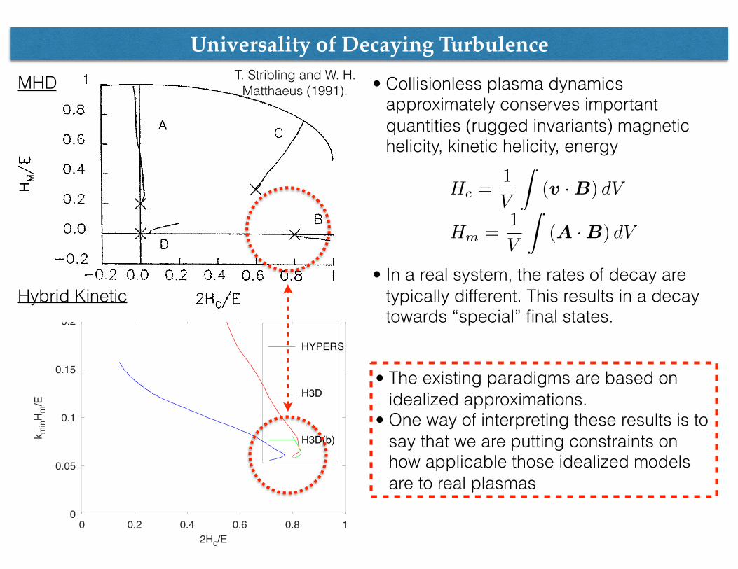
T. Stribling and W. H. Matthaeus (1991).
Universality of Decaying Turbulence
• Collisionless plasma dynamics approximately conserves important quantities (rugged invariants) magnetic helicity, kinetic helicity, energy
Hc =1
V
Z(v ·B) dV
Hm =1
V
Z(A ·B) dV
• In a real system, the rates of decay are typically different. This results in a decay towards “special” final states.
MHD
Hybrid Kinetic
• The existing paradigms are based on idealized approximations.
• One way of interpreting these results is to say that we are putting constraints on how applicable those idealized models are to real plasmas

Sub-Proton Range in low-β plasma: Fully-Kinetic Simulations
Magnetosheric Multi Scale (MMS) [NASA]
C. H. K. Chen and S. Boldyrev, 2017
4
10-810-710-610-510-410-310-210-1100101
PSD
(nT
2/H
z)
-3.59
kd i
=1
kρi=
1
kd e
=1
kρe=
1
δB⊥
δB∥
100 101 102
fsc (Hz)
10-1
100δB
2 ∥/δB
2 ⊥
FIG. 4. Power spectra of δB∥ and δB⊥ and magnetic compressibil-
ity δB2
∥/δB2
⊥. In the lower panel, the black dotted lines show the
asymptotic predictions 1/(1 + 2/βi) and 1, and the red solid line isEq. (6). Vertical dashed lines are the same as in Figure 3; the addi-tional magenta line is the transition scale [Eq. (4)].
To understand the nonlinear properties of inertial kineticAlfven turbulence, we turn to the dynamical equations. Un-der the ordering assumption k∥/k⊥ ∼ δB/B0 ∼ δn/n0 ∼ω/Ωe ≪ 1, and Te ≪ Ti (so that the electron pressure andelectron gyroradius effects can be neglected), fluctuations inthe scale range 1/ρi ≪ k⊥ ≪ 1/ρe and frequency rangek∥vth,e ≪ ω ≪ k⊥vth,i are described by the equations
∂
∂t
(
1−∇2⊥
)
ψ + [(z ×∇δn) ·∇]∇2⊥ψ = −∇∥δn, (7)
∂
∂t
(
1 +2
βi−∇2
⊥
)
δn+[(z ×∇δn) ·∇]∇2⊥δn = ∇∥∇2
⊥ψ,
(8)where ψ is the flux function δB⊥ = z × ∇ψ, and ∇∥ =∂/∂z + (z ×∇ψ) · ∇⊥ is the gradient along the instanta-neous local magnetic field direction. Dimensionless vari-ables, t′ = t|Ωe|, x′ = x/de, ψ′ = ψ/(deB0), and δn′ =(βi/2)(δn/n0), have been used here (with the primes omit-ted). The derivation of these equations is given in the Sup-plemental Material [59]. For k⊥ ≪ 1, the nonlinearities inthe left hand sides of Eqs. (7)-(8) can be neglected, and fork⊥ ≫
√
1 + 2/βi, the nonlinearities in the right-hand sides,i.e., the nonlinear parts of ∇∥, can be neglected. Withoutany of the nonlinear terms, the inertial kinetic Alfven wave[Eq. (5)] is obtained.
In the absence of energy supply and dissipation, the equa-tions conserve the energy
E =
∫[
δn
(
1 +2
βi−∇2
⊥
)
δn−∇2⊥ψ
(
1−∇2⊥
)
ψ
]
d3x.
(9)In a turbulent state, both terms of E are of the same order.For scales k⊥ ≫
√
1 + 2/βi, this means that δnλ ∼ ψλ/λ,
where δnλ and ψλ denote the typical fluctuations of the fieldsat the scale λ across the background magnetic field. In thesame limit, the nonlinearity is dominated by the terms in theleft-hand sides of Eqs. (7)-(8), and the nonlinear time canbe estimated as τ ∼ λ2/δnλ. Assuming a constant energyflux through scales, ε ∼ (δn2
λ/λ2)/τ ∼ δn3
λ/λ4, leads to
the scaling of the density and magnetic fluctuations δnλ ∼ψλ/λ ∼ ε1/3λ4/3, and their field-perpendicular energy spec-
trum En,B(k⊥) ∝ k−11/3⊥ . This is close to the measured slope
in Figure 4, which shows a spectral index of −3.6 for the δB⊥
fluctuations between kde ≈ 1 and kρe ≈ 1. While a similarspectrum has been derived for whistler turbulence [63–65],the measurements here indicate that the turbulence is inertialkinetic Alfven in nature.
The anisotropy implied by the critical balance condition canalso be determined. Balancing the linear and nonlinear termsin Eqs. (7)-(8), ψλ/(lλ2) ∼ δn2
λ/λ4, we obtain the relation
between the parallel and perpendicular scales l ∼ λ5/3. InFourier space this means that the turbulent energy is concen-
trated in the region k∥ <∼ k5/3⊥ . This region becomes pro-gressively broader in k∥ and less anisotropic as k⊥ increases.This suggests, therefore, that in contrast to standard Alfvenand kinetic Alfven turbulence, the energy cascade in inertialkinetic Alfven turbulence supplies energy more efficiently tok∥ rather than k⊥ modes.
Discussion.—We have presented new high resolution mea-surements of kinetic scale turbulence in the Earth’s magne-tosheath. In the first decade of the kinetic range, the tur-bulence is similar to that in the upstream solar wind; low-frequency (ω ≪ k⊥vth,i), anisotropic (k⊥ ≫ k∥), and ki-netic Alfven in nature, with spectra that match theoreticalpredictions and numerical simulations. In the second decade,the turbulence becomes inertial kinetic Alfven, identified hereby the increase in magnetic compressibility matching that ofthe inertial kinetic Alfven wave [Eq. (6)]. The nonlinear
equations [Eqs. (7)-(8)] suggest a k−11/3⊥ spectrum of mag-
netic fluctuations between the electron inertial scale and elec-tron gyroscale, consistent with the observations. Interestingly,this turbulence is expected to exhibit a qualitatively differentanisotropy to standard Alfven and kinetic Alfven turbulence,becoming less anisotropic towards smaller scales. We planto investigate these aspects further through numerical simula-tions of Eqs. (7)-(8) and further observations.
As well as in the magnetosheath, inertial kinetic Alfven tur-bulence is likely to be relevant in a variety of other astrophys-ical environments, where the ions are often much hotter thanthe electrons. For example, the fast solar wind model of Chan-dran et al. [66] predicts βi ∼ 0.2 and βe ∼ 0.02 at 10 Solarradii from the Sun, a region of the corona which will soon bemeasured by the Solar Probe Plus spacecraft [67]. Similarly,in hot accretion flows, where turbulent heating is thought tobe important, the ions are likely to be much hotter than theelectrons [68]. In addittion, collisionless shocks are commonthroughout the universe, leading to regions with large ion tem-peratures [69, 70]. Inertial kinetic Alfven turbulence, there-
Spectrum of Magnetic Fluctuations in the Earth’s Magnetosheath
“fingerprint” of fluctuations
The nature of fluctuations
changes
transition 1 transition 2
simple analysis
10-9
10-8
10-7
10-6
10-5
10-4
10-3
10-2
|B|||2
|B⊥|2
k-2.8
k-4.2
100
10-1 100
kde
|B||/B⊥|2
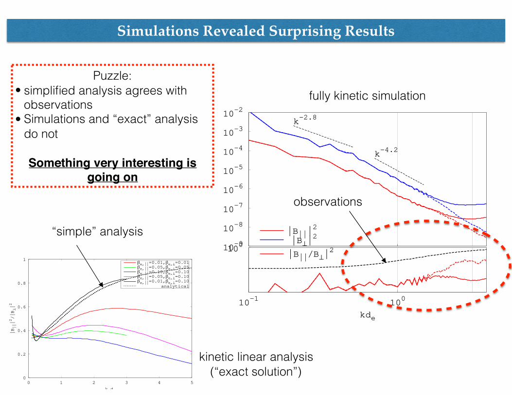
Simulations Revealed Surprising Results
fully kinetic simulation
0
0.2
0.4
0.6
0.8
1
0 1 2 3 4 5
|B|||2/|B⊥|2
k⊥de
βe,||=0.01,βe,⊥=0.01βe,||=0.05,βe,⊥=0.05βe,||=0.10,βe,⊥=0.10βe,||=0.05,βe,⊥=0.10βe,||=0.01,βe,⊥=0.10
analytical
Puzzle: • simplified analysis agrees with
observations • Simulations and “exact” analysis
do not
Something very interesting is going on
“simple” analysis
observations
kinetic linear analysis (“exact solution”)

Summary
1.Understanding of plasma turbulence is a grand challenge problem.
2.We are using Blue Waters to study some aspects of this problem, namely
kinetic effects associated with turbulence dissipation.
3.Year 1 has yielded exciting results, some of them await explanation
J. Podesta and V. Roytershteyn, “The most intense electrical currents in the solar wind: Comparisons between single spacecraft measurements and plasma turbulence simulations”, under review in JGR
3 more manuscripts in preparation
1 new project has just began with the simulation data produced in BW
Database of large-scale simulations to be used for years to come (hopefully).
Publications & data products