Dissipative Partial Differential Equations andDynamical Systems

C.E. Wayne

October 31, 2012

Abstract

This article surveys some recent applications of ideas from dynamical sys-tems theory to understand the qualitative behavior of solutions of dissipativepartial differential equations with a particular emphasis on the two-dimensionalNavier-Stokes equations.

1 Introduction

The focus of this article is the application of dynamical systems ideas to the study ofdissipative partial differential equations. The notion of dissipativity arises in physicswhere it is generally thought of as a dissipation of some “energy” associated withthe system and such systems are contrasted with energy conserving systems likeHamiltonian systems. In finite dimensional systems, the notion of dissipativity isrelatively easy to quantify. If we have a system of ordinary differential equations(ODEs) defined on Rn,

xj = fj(x) = fj(x1, . . . , xn) , j = 1, . . . n , (1)

then a common definition of dissipativity is that there be some bounded set, B, whichis forward invariant under the flow defined by our differential equations and such thatevery solution of the system of ODEs eventually enters B, [Hal88]. Such a set isreferred to as an absorbing set. If an absorbing set exists, and if φt is the flow definedby this dynamical system, then we can define an attractor for the system by

A = ∩t≥0φt(B) , (2)

which will be compact and invariant, and will have the property that any trajectorywill approach this set as t→∞.

1

Another property often associated with dissipativity is that the determinant ofthe Jacobian of the vectorfield in (1) is negative, i.e.

det

( ∂fj∂xkj,k=1,...,n

)< 0 . (3)

If this determinant is zero, then the system conserves phase space volumes, and this isone of the properties associated with Hamiltonian systems. Condition (3) means thatthe systems “dissipates” phase space volume, but note that it is not, in itself, sufficientto insure that we have a bounded attractor for the system, as the two dimensionalexample

x1 =1

2x1 , x2 = −x2 , (4)

for which almost every solution tends to infinity shows. However, if the systemsatisfies (3), and is in addition dissipative in the sense described above, then wecan immediately conclude that the attractor for the system has zero n-dimensionalvolume. Thus, the asymptotic behavior of the system is determined by what happenson a very “small” set.

One important direction of research in the study of dissipative systems is to focuson the properties of the attractor. In special cases, the attractor may consist of asmall number of simple orbits, like stationary solutions and their connecting orbits, orperiodic orbits. In other, more complicated cases, the attractor may contain chaotictrajectories but it may itself live in a manifold of much lower dimension than thenumber of degrees of freedom of our original system. In such circumstances, thelong-time behavior of arbitrary solutions of the original system can be determinedfrom a study of the possibly much smaller system obtained by restricting the originalODEs to this manifold containing the attractor. This dimensional reduction has beena powerful tool in the study of dissipative systems.

When one turns from ODEs to partial differential equations (PDEs), the discussionbecomes more complicated due to the infinite dimensional nature of the problem. Forone thing, the long-term behavior of the system may well depend on the norm wechoose on our space of solutions. However, even after one has fixed the norm on thesystem the situation can be problematic due to the fact that closed and boundedsets need no longer be compact. Thus, even if we find some bounded absorbingset B, as above, we have no guarantee that ∩t≥0φt(B) will be non-empty! Thus,in addition to proving that the PDE is well-posed, one typically needs to establishsome smoothing properties to show that not only is there a set B that eventually“absorbs” all trajectories but also that this set is precompact in the function spaceon which we are working. Fortunately, this smoothing can often be proven for the sortof dissipative systems we discuss here and the systems described in the subsequentsections all have well defined attractors.

The reduction of dimension of the problem which results from focussing one’sattention on the restriction of the system to the attractor is an even more powerful

2

tool in the context of PDEs than ODEs. As we will see in subsequent sections,many physically interesting PDEs have attractors of finite (sometimes even small)dimension. Thus, the complex behavior of solutions of the PDE can be captured bythe behavior of the solutions restricted to this finite dimensional set.

In one sense this simply transfers the problem from the study of the infinite dimen-sional behavior of solutions of the PDE to computing the possibly very complicatedstructure of the attractor and the latter question remains an active and open areaof research for many of even the most natural physical systems, but it is at least afinite dimensional question and one that is well suited to attack with the methods ofdynamical systems theory.

As mentioned above, in infinite dimensional systems, dissipativity requires morethan simply the existence of a bounded absorbing set to insure that the system hasan attractor. There are several additional hypotheses one can make to insure thenecessary compactness - see [Hal88] or [Tem88], for example. However, we followRobinson ([Rob01], p. 264) and define:

Definition 1. A semigroup is dissipative if it possesses a compact absorbing set B.

The drawback of this definition is that one must always check the compactness ofthe absorbing set.

Given a dissipative semigroup φt on a Banach space X, the ω-limit set of a setU ⊂ X is

ω(U) = u ∈ X | there exists u0 ∈ U, and tn, tn →∞,such that lim

n→∞‖φtn(u0)− u‖ = 0 . (5)

A global attractor is then defined as ([Tem88], p. 21)

Definition 2. A set A ⊂ X is a global attractor for the semiflow φt, if

1. A is invariant.

2. Every bounded set is uniformly attracted to A. That is to say, if U ⊂ X isbounded, then

limt→∞

dist(φt(U),A) = 0 . (6)

With these definitions it is relatively easy to show:

Theorem 1. If the semiflow φt is dissipative it has a universal attractor. If B is acompact absorbing set for φt, then the attractor is ω(B).

Proof. The proof is relatively straightforward. The sets A(t0) = ∪t≥t0φt(B) are non-empty, compact and decreasing, and their intersection, which gives ω(B) is clearlyinvariant under φt and one checks the attractivity property by contradiction. Thedetails are in [Rob01].

3

Remark 1. For a semiflow defined by a well-posed PDE such that φt(u0) = φt(v0)implies u0 = v0, one has the important corollary that when restricted to the attractor,φt actually defines a flow, not just a semi-flow. That is, if u0 ∈ A, then φt(u0) isdefined for all t ∈ R, not just for t ≥ 0. This is somewhat surprising since in generalit is not possible to solve dissipative PDEs “backwards” in time.

One may wonder how hard it is to establish that an infinite dimensional dynamicalis dissipative in the sense of Definition 1. Often the compactness needed in thedefinition follows in a relatively straightforward way from the same sorts of estimatesthat yield existence and uniqueness of solutions. Consider, for example, the family ofnon-linear heat-equations

ut = uxx + g(u) , 0 < x < L (7)

with zero boundary conditions - i.e. u(0, t) = u(L, t) = 0. If one places mild growthconditions on the nonlinear term g this is known as the Chafee-Infante equation andwas one of the first PDE to be systematically studied with the methods of dynamicalsystems theory. If one assumes that the initial conditions u0 ∈ H1

0 (0, L), then themethods of semigroup theory readily show that the orbit u(·, t) with this initial condi-tion is relatively compact in this Hilbert space [Mik98], and one has an absorbing set.Hence the equation defines a dissipative dynamical system in the sense of the abovedefinition. In this case the attractor is quite simple - for a special class of nonlinearterms, Henry showed that it consisted of the stationary solutions of the equation, andtheir unstable manifolds, [Hen81].

Of course, the converse is of this fact is also true - there are equations like thethree-dimensional Navier-Stokes equation which are expected to be dissipative onphysical grounds, but the fact that there is no proof that smooth solutions exist forall time for general initial data precludes proving that they are dissipative in the senseof the previous definition.

The main example of an infinite dimensional dissipative system that we’ll examinein the remainder of this review is the two-dimensional Navier-Stokes equation (2DNSE). These equations describe the evolution of the velocity of a two-dimensionalfluid. While it may seem unrealistic to study two-dimensional fluid flows in a three-dimensional world there are a number of circumstances (e.g. the Earth’s atmosphere)where this is a reasonable physical approximation. For further discussion of this point,see [Way11].

Physically, the NSE arise from an application of Newton’s law for the fluid, namely

d

dt(momentum) = applied forces . (8)

If u(x, t) is the fluid velocity, and if we assume that the fluid is incompressible so thatwe can take the density to be constant, the time rate of change of the momentum isgiven by the convective derivative

d

dt(momentum) = ρ

∂u

∂t+ ρu · ∇u . (9)

4

The second term in this expression reflects the fact that the momentum of a smallregion of the fluid can change not only due to changes in its velocity, but also becauseit is being simultaneously swept along by the background flow.

The forced are are typically split into three parts:

• forces due to pressure: fpressure = −∇p(x, t), where p is the pressure in the fluid.

• viscous forces: These involve modeling internal properties of the fluid. We willtake a standard model which says fvisc = α∆u, for some constant α.

• external forces, which we denote by g.

If we insert these expressions into Newton’s law, we obtain

∂tu + u · ∇u = (α/ρ)∆u =1

ρ∇p+

1

ρg. (10)

Note that if we consider a fluid moving in d dimensions, this expression is actually asystem of d partial differential equations. However, we have d+ 1 unknown functions- the d components of the velocity, plus the pressure. To close our system we appendthe additional equation

∇ · u = 0 , (11)

which reflects the assumption that the fluid is incompressible. For a further discussionof the physical origin of these equations, one can consult [DG95].

As remarked above for the three-dimensional case it is not known whether or notthe NSE possess smooth solutions for all times, even if one assumes that the initialvelocity field is very smooth and there are no external forces acting on the system.Indeed, this is one of the famous Millennium Prize Problems. Thus, we will discussonly two dimensional fluids, i.e. we will assume that

u = u(x, t) ∈ R2 , for x ∈ Ω ⊂ R2 . (12)

In order to complete the specification of the problem, we must supplement equations(10)-(11) with appropriate boundary conditions. We’ll focus on two special caseswhich are especially amenable to mathematical analysis, namely either

1. Ω = R2, with boundary conditions imposed by assuming appropriate decayconditions on u at infinity, or

2. Ω = [−π, π]×[−(πδ), (πδ)] = T2δ with periodic boundary conditions, i.e. u(x1, x2, t) =

u(x1 + 2π, x2, t) = u(x1, x2 + 2πδ, t). Note that δ is a parameter that measuresthe asymmetry of our domain - it is assumed to be O(1) and is not necessarilysmall.

5

Very early in the study of fluid mechanics it was pointed out by Helmholtz that itwas often more useful to study the evolution of the fluid’s vorticity than its velocity.The vorticity is defined by the curl of the velocity field - i.e. ω(x, t) = ∇×u(x, t) andin general it is a vector, like the velocity. However, in two-dimensions an importantsimplification occurs:

ω(x1, x2, t) = (0, 0, ∂x1u2 − ∂x2u1) = (0, 0, ω(x1, x2, t)) (13)

so we see that only one component of the vorticity is non-zero and we can treat it asa scalar. If we take the curl of (10) we see that in two dimensions, we arrive at thescalar PDE

∂tω + u · ∇ω = ν∆ω + f , (14)

here the parameter ν = α/ρ, and f = 1ρ(∂x1g2 − ∂x2g1).

One advantage of this formulation of the problem is that the pressure term hasdisappeared entirely from the equation. However, the price we pay is that it appearsat first that the equation is no longer well defined - the velocity u still appears in theequation, although we have no equation for its evolution. However, we can eliminateu from the equation by recalling that

• u is divergence free, and

• ω is the curl of u.

This means that we can reconstruct u from the vorticity with the aid of Biot-Savartlaw, which in two-dimensions takes the form

u(x, t) = B[ω](x, t) =1

2π

∫y⊥

|y|2ω(x− y, t)dy =

1

2π

∫(x− y)⊥

|x− y|2ω(y, t)dy , (15)

where, if y = (y1, y2), y⊥ = (−y2, y1).If we insert this representation into (14), we see that we can regard the vorticity

equation:∂tω = ν∆ω −B[ω] · ∇ω + f , (16)

as a nonlinear heat equation, with a quadratic, but non-local, nonlinear term. Thisrelationship with the heat equation, and in particular the fact that this means thatthe vorticity of two-dimensional flows satisfies a maximum principle will be used insubsequent sections.

In remaining sections we will discuss how dynamical systems ideas can be appliedto dissipative PDEs, taking (16) as our principal example. It is perhaps not surprisingthat this equation defines a dissipative dynamical system given the relationship withthe heat equation, which models the dissipation of heat energy in physical systems.We will verify the dissipativity in the sense of Definition 1 in a later section andsee how ideas like invariant manifold theory and Lyapunov functions can give manyinsights into details of the behavior of its solutions.

6

2 The ω-limit set of the two-dimensional Navier-

Stokes equation

In this section we focus on the long-time asymptotic behavior of solutions of theunforced two-dimensional vorticity equation

∂tω = ν∆ω − u · ∇ω (17)

defined on the whole plane - i.e. ω = ω(x, t), x ∈ R2. At first glance, it may seemthat this equation is unlikely to yield interesting dynamics – the dissipation in theequation might be expected to dampen out any nontrivial motions. However, wewill see that in the case of both bounded and unbounded domains, characteristicstructures emerge in the solutions which numerical investigations indicate are alsoimportant features of two-dimensional forced flows.

Clearly, ω ≡ 0 is a fixed point for this equation and from a dynamical systemspoint of view it is natural in this circumstance to linearize about the fixed point andask what the linearization tells us about the behavior nearby. If we linearize the 2Dvorticity equation about the zero solution the resulting linearized equation is the 2Dheat equation:

∂tω = ν∆ω . (18)

Approaching this problem from a dynamical systems perspective a natural next stepwould be to construct center/stable/unstable manifolds for the nonlinear equationwhich correspond to the eigenspaces of the linear problem with eigenvalues havingzero, negative or positive real parts respectively.

Unfortunately we immediately face a problem if we attempt to apply those ideasin the present context. One can easily compute the spectrum of the linear operatoron the RHS of the heat equation using the Fourier transform and one finds that thespectrum consists of the negative real axis, up to and including the origin. Sincethere is no gap in the spectrum there is no way to split the phase space into “center”or “stable” parts as required in the center manifold theorem and no obvious way ofidentifying the modes associated with particular decay properties.

A way of circumventing this difficulty emerges if we recall the form of the funda-mental solution of the heat equation:

Gν(x, t) =1

4πνte−|x|

2/(4νt) . (19)

This suggests that it may be natural to consider (17) not in the variables (x, t), butin new variables in which x and t are related as ∼ x/

√t. With this in mind, we

introduce new independent and dependent variables:

ω(x, t) =1

(1 + νt)w(

x√1 + νt

, log(1 + νt)) (20)

ξ =x√

1 + νt, τ = log(1 + νt)

7

Remark 2. These types of variables are often used in studying parabolic PDE wherethey are sometimes referred to as scaling variables.

If we now rewrite (18) in terms of these new variables we obtain the new PDE

∂τw = Lw , w = w(ξ, t) , ξ ∈ R2 (21)

Lw = ∆ξw +1

2ξ · ∇ξw + w = ∆ξw +

1

2∇ξ · (ξw)

At first sight, it may not be apparent why (21) is an improvement over (18) as wehave made the equation more, rather than less, complicated. However, as we showbelow, in contrast to the Laplace operator which appears on the right hand side ofthe heat equation, the operator L has a gap in its spectrum between the part of thespectrum with zero real part and the remainder and this will allow us to apply thecenter-manifold theorem to understand the asymptotic behavior of solutions near thefixed point at the origin.

To understand the spectrum of L, consider the eigenvalue problem

Lψλ = λψλ . (22)

If we separate variables in this PDE, we get a pair of ordinary differential equationsof the form

d

dξ21φλ +

1

2

d

dξ1(ξ1φλ) = λφλ , (23)

with a similar equation for the ξ2 part of the solution. Taking the Fourier transformof this equation yields

− k2φλ −1

2kd

dkφλ = λφλ . (24)

This first order equation can be solved with the aid of integrating factors and onefinds that for any λ ∈ C one has a solution:

φλ(k) =C+

|k|2λe−k

2

H(k) +C−

|k|2λe−k

2

H(−k) (25)

where H(k) is the Heaviside function and the fact that we have two constants ofintegration for a first order differential equation reflects the singular point at k = 0.

At first sight, this seems as if every point λ is in the spectrum of L. However,recall that the spectrum of an operator depends on the space on which it acts. Inparticular, if <(λ) > 0, the functions in (25) “blow-up” at k = 0 and hence won’t bein any well behaved function space. In order to say exactly what the spectrum of L is,we must decide what function space it acts on - like many operators, its spectrum willchange, according to the domain chosen. It has long been known that the time-decay

8

of solutions of parabolic PDEs is linked to the spatial decay rate of their solutions.With this in mind, we define a family of weighted Sobolev spaces:

L2(m) = f ∈ L2(R2) | ‖f‖m <∞

‖f‖m =

(∫R2

(1 + |ξ|2)m|f(ξ)|2dξ)1/2

(26)

Hs(m) = f ∈ L2(m) | ∂αf ∈ L2(m) for all α = (α1, . . . , αd) with |α| ≤ s

One reason that these spaces are so convenient for our purposes is the fact thatFourier transformation turns differentiation into multiplication and vice-versa. Forthese spaces, that makes it easy to check that for any non-negative integers s and m,Fourier transformation is an isomorphism between Hs(m) and Hm(s), i.e. a functionf is in Hs(m), if and only if its Fourier transform f ∈ Hm(s).

Applying this observation to the expression for φλ in (25), we see that due to thesingularity at k = 0 and the rapid decay as |k| → ∞, φλ ∈ Hm(s) if the first mderivatives of φλ are square integrable in some neighborhood of the origin.

Note that there are some “special” values of λ. If λ = 0,−1/2,−1,−3/2, . . . , wecan choose A± so that φ−n/2(k) = Akn exp(−k2). These are entire, rapidly decayingfunctions and thus are elements of Hm(s) for any values of m and s, so that the non-negative half integers are eigenvalues of L for any s and m, with eigenfunctions givenby the inverse Fourier transform of these expressions. In particular, we see that λ = 0is always an eigenvalue and its eigenfunction is the Gaussian φ0(ξ) = C0 exp(−ξ2/4).For non-half integral values of λ, we cannot choose the constants A± to make theeigenfunctions smooth, and thus, at least for some values of s, they will not be inthe spaces Hm(s). In fact, one can easily verify that in one-dimension, for no valueof λ ∈ C with <(λ) ≥ 0 will φλ be in H1(s), because the derivative will have anon-square-integrable singularity at the origin. In two-dimensions, one can tolerateslightly worse singularities, but one still finds that no φλ with <(λ) ≥ 0 will lie inH2(s). A careful examination of this argument allows one to compute exactly whatthe spectrum of L is and one finds

Theorem 2. ([GW02], Theorem A.1)Fix m > 1 and let L be the operator in (21)acting on its maximal domain in L2(m). Then

σ(L) =

λ ∈ C | Re(λ) <

1

2− m

2

∪−n

2| n = 0, 1, 2, . . .

.

The key fact here, from the point of view of dynamical systems theory, it thatwe have now created a spectral gap. So long as we choose the decay rate parameterm ≥ 2 in our function space, the eigenvalue λ = 0 is an isolated point in the spectrumof L, with all the rest of the spectrum lying strictly in the left half plane. Thus, atleast intuitively, we can now hope to define the center subspace of the linear problemto be the span of the eigenfunction(s) of the zero eigenvalue, the stable subspace to be

9

the spectral subspace corresponding to the remainder of the spectrum, and attemptto construct a center-manifold for the full nonlinear equation that it is tangent to thezero-eigenspace at the origin.

We first note that the zero-eigenspace is very simple in this case - it is one-dimensional and consists just of the span of the Gaussian function

φ0(ξ) =1

4πe−ξ

2/4 . (27)

For future reference we note that the projection onto this eigenspace is given by thezero eigenfunction to the adjoint operator to L, namely

L†v = ν∆v − 1

2ξ · ∇v . (28)

The constant function is clearly a zero eigenfunction for L† and consequently, theprojection of f ∈ H2(m) onto the zero eigenspace of L is given just by P0f =(∫R2 f(ξ)dξ)φ0.

While the spectral gap in the spectrum of the linear part of the equation makes itreasonable to expect that there will be an center manifold for the semi-flow definedby the 2D NSE, there are technical difficulties associated with constructing invariantmanifolds for PDE that still must be overcome. In contrast to the case of ordinarydifferential equations where it is more or less clear what the optimal assumptions onthe vectorfield should be in order to obtain an invariant manifold theorem, the situa-tion is far less clear in the case of PDE. For instance, depending on the circumstances,it may be preferable to assume that the semi-group associated with the linear part ofthe equation may be more or less smoothing. Depending on the choices made in thiscase, one may need to make either stronger hypotheses about the nonlinear part of theequation, or draw weaker conclusions about the manifold one constructs. There is farless of a “one size fits all” invariant manifold theorem in infinite dimensional systems- instead one typically tailors the hypotheses of the theorem to the circumstances ofinterest. For some of the choices that have been made, see [BJ89], [Mie91] or [VI92].One general principle that seems to emerge from these different contexts is that it isoften easier to work with the semi-flow defined by the PDE, rather than the equationitself, if this semi-flow exists. This is because it already incorporates any smoothingassociated with the linear evolution, and we don’t need to worry about precisely whatsmoothing assumptions to make on the flow. (For instance, one common assumptionis that the linear part of the equation defines an analytic semi-group, but while sucha hypothesis would apply to the vorticity equation (14), it would no longer hold oncewe rewrite the equation in terms of the scaling variables (20).)

One infinite dimensional version of the center-manifold theorem that does applyto our problem is the version due to Chen, Hale and Tan (CHT) [CHT97]. (CHT)assume that the PDE defines a semi-flow φt on some Banach space, X. They thenmake four natural hypotheses about this semi-flow. We refer the reader to the originalpaper for the details on these assumptions, but roughly they are as follows:

10

(H1) φt(u) is Lipshitz continuous in both t and u with uniformly bounded Lipshitzconstant for t in some interval.

(H2) For some fixed, positive τ , φτ can be split into a bounded linear operator anda globally Lipshitz operator.

(H3) The Banach space can be split into a direct sum of two pieces (a “center”subspace, X1 and a “stable” subspace X2) and when the linear part of φτ

acts on the stable subspace it produces decay at a faster rate than the growthproduced when the inverse of the linear part of φτ acts on the center subspace.(This is a reflection and consequence of a spectral gap in the spectrum of thelinear part of the PDE.)

(H4) The ratio of the Lipshitz constant of the nonlinear term divided by the spectralgap must be small.

Assuming that these hypotheses are satisfied, (CHT) then prove the following:

• There exists a Lipshitz function g : X1 → X2 whose graph is invariant withrespect to φτ . This is the center manifold for our system.

• Any orbit of φτ will approach an orbit on the center manifold as time goes toinfinity.

We will apply the (CHT) theorem to the two-dimensional vorticity equation, (17),rewritten in terms of the scaling variables (20). In addition to redefining the depen-dent vorticity variable ω as in (20) we also rescale the velocity variable as

u(x, t) =1√

1 + νtv(

x√1 + νt

, log(1 + νt)) . (29)

Remark 3. With this definition one can check that the rescaled vorticity w andrescaled velocity v are still related to one another through the Biot-Savart law.

If we rewrite (17) in terms of these new variables we find

∂τw = Lw − 1

νv · ∇ξw . (30)

If we take initial condition w|τ=0 = w0, we can define the semi-group associated with(30) with the aid of DuHamel’s formula as

w(τ) = eτLw0 −1

ν

∫ τ

0

e(τ−s)L(v(s) · ∇ξw(s))dx . (31)

The two terms in (31) define the splitting into linear and nonlinear pieces in hypothesis(H2), and the decay hypotheses of (H3) are intuitively satisfied due to the gap in

11

the spectrum of L. One can check them rigorously just by noting that the semigroupetL is just the heat semigroup written in terms of the scaling variables. Expressingthe heat semigroup in terms of these variables then leads to the expected estimates,[GW02].

The remaining hypotheses (H1) and (H4) as well as the second part of (H2)concern the smoothness of the nonlinear term. In order to treat this term, one needsestimates that allow us to transfer information about the vorticity field to informationabout the velocity field. The types of estimates we will need are analogous to theHardy-Little-Sobolev (HLS) inequality, [LL97]. Note that from (15), we have

|vj(x)| ≤ 1

2π

∫R2

1

|x− y||w(x− y)|dy . (32)

Thus, if w ∈ Lp(R2), the HLS inequality immediately implies that

‖u‖Lq ≤ C‖ω‖Lp , (33)

for q = 2p/(2− p). We need to refine these inequalities to account for the weights inour function spaces (i.e. to account for the fact that we work not in L2, but in L2(m)),but very similar estimates hold in that case. An extensive set of such inequalities isproved in ([GW02], Appendix B).

These inequalities allow one to establish the Lipshitz bounds used in (H1) and(H4). However, they would not immediately lead the global Lipshitz estimate requiredin the second part of (H2). This is obtained as in other constructions of the center-manifold theorem by “cutting off” the nonlinear term outside of some ball centeredat the origin. More precisely we multiply the nonlinear term by χ(‖w‖L2(m)), where χis a smooth function equal to one on a neighborhood of zero and vanishing outside ofsome slightly larger neighborhood. This results in an equation whose nonlinear termnow has a global Lipshitz bound and whose solutions agree with those of our originalequation whenever ‖w‖L2(m) is sufficiently small. Again, the details are provided in[GW02].

The estimates above allow us to apply the (CHT) theorem to construct a one-dimensional center manifold for the two-dimensional vorticity equation, written interms of the scaling variables as in (30). Furthermore, the (CHT) theorem alsoguarantees that all solutions of the equation which remain in some neighborhood ofthe origin will approach an orbit on the center manifold. (We note that this restrictionto solutions near the origin is not contained in the statement of the (CHT) theoremabove. It results from the fact that we had to cut-off the nonlinear term in (30)in order to verify the hypotheses of the theorem, and hence the conclusions of thetheorem only apply to solution that remain in the region where the cutoff function isone.) Thus, all the long-time asymptotics of such solutions will be determined by theorbits on the center manifold, so our next step is to compute the dynamics of (30)when restricted to this manifold. In the vorticity equation the center subspace, X1

12

is just the span of the eigenfunction of the zero eigenvalue which we showed aboveis the Gaussian function φ0 - i.e. any function wc ∈ X1 has the form αφ0. Thus,any point in the center manifold can be written as w = αφ0 + g(α), where g is thefunction whose graph defines the center manifold, and the restriction of (30) to thecenter manifold can be written as

αφ0 = P0(N(αφ0 + g(α))) . (34)

Here, N is short-hand notation for the nonlinear term in (30), P0 is the projection ontothe center subspace, and there is no linear term in the equation because the eigenvaluecorresponding to φ0 which would give rise to the linear term in the equation is zero.Recall that as we showed just after (28), the projection of a function f onto the centersubspace is given by multiplying by φ0 by the integral of f over R2. Thus, we needto integrate the nonlinear term in (30) over R2 - i.e.

− 1

ν

∫R2

(v · ∇w)dξ (35)

But if we recall that v is incompressible, i.e. has zero divergence, we can rewrite theintegrand in this expression as ∇ · (vw), and then the integral vanishes due to thedivergence theorem! Thus, the restriction of (30) to the center manifold is simply

α = 0 . (36)

This implies the surprising fact that the center manifold consists entirely of fixedpoints! Even more surprising, we can write them down explicitly - they are justmultiples of the Gaussian. That is, if we take

w(ξ, τ) = OA(ξ, τ) =A

4πe−|ξ|

2/4 (37)

this is a fixed point of (30) for all values of A. The reason is that if one computes thevelocity field corresponding to OA from the Biot-Savart law it is

vA(ξ, τ) =A

2π

ξ⊥

|ξ|2(

1− e−|ξ|2/4). (38)

Note that this velocity field is a purely tangential vector field, while OA is purelyradial and as a consequence, vA · ∇OA ≡ 0. Recalling that Lφ0 = 0, since φ0 isthe eigenfunction with eigenvalue zero, we see that the RHS of (30) vanishes whenevaluated at OA and as a consequence these are all fixed points of the equation.

Remark 4. These solutions of the two-dimensional Navier-Stokes equation have beenknown for a long time and are called Lamb-Oseen vortices. If expressed in terms ofthe original variables instead of the scaling variables, they are self-similar solutionsof the equation, rather than fixed points.

13

Remark 5. We can use the (CHT) theorem to construct other invariant manifolds,besides just the center manifold. Recall the computation of the spectrum in Theorem2. If we choose the decay rate m of our function space m ≥ 3, we see that there arenow two isolated eigenvalues in addition to the essential spectrum - namely λ0 = 0 andλ1 = −1/2. If one examines the eigenfunctions computed above, one finds that −1/2is a double eigenvalue and its eigenfunctions are Hermite functions, C1ξ1e

−|ξ|2/4 andC1ξ2e

−|ξ|2/4, where the constant C1 is chosen to normalize the eigenfunctions. Onecan then reapply the (CHT) theorem, this time taking as the “center” subspace X1, thethree dimensional space spanned by the Gaussian and these two Hermite functions.This gives rise to a three dimensional invariant manifold, and just as above one cancompute explicitly the system of ordinary differential equations that results when onerestricts (30) to this manifold. This computation uses the fact that the eigenfunctionsof the adjoint operator L† with eigenvalues −1/2 are just the coordinate functions ξ1and ξ2 and hence the projection onto these directions corresponds just to taking firstmoments of the solution. By choosing larger and larger values of m, one can exposemore and more isolated eigenvalues, and one finds that their eigenfunctions are alsogiven by Hermite functions of higher and higher order, and the projections onto theseeigendirections are given by combinations of higher order moments of the solution.

Remark 6. There has been a fair amount of work using more traditional PDE tech-niques to identify special families of solutions of the Navier-Stokes equations whichhave specific temporal decay properties. For instance, Mayakawa and Schonbek [MS01]gave necessary and sufficient conditions for solutions to satisfy specific temporal decayrates in terms of integrals of various moments of the solutions. From the dynamicalsystems point of view, we see that solutions decaying with a particular rate can beidentified as lying in a particular invariant manifold. For example, any solution ap-proaching a non-zero Oseen vortex in the center manifold will decay in time with thesame rate as the Oseen vortex, i.e. ∼ t−1/2 in the L∞ norm in the original, unscaledvariables. The only way a solution in a neighborhood of the origin can avoid ap-proaching one of the Oseen vortices is if it lies in the invariant manifold of solutionsasymptotic to the origin. (These manifolds are sometimes called Fenichel fibers, andthey consist of all solutions sharing the same long-time asymptotics.) As we notedin the preceding remark, the projections onto the various eigenspaces are expressed asmoments of the solution. Gallay and I were able to show that the condition that asolution lay on the Fenichel fiber through the origin was exactly the same conditionon the moments that had earlier been found by analytic means in [MS01].

Remark 7. In Remark 5 we observed that the Hermite functions are eigenfunctionscorresponding to the isolated eigenvalues of L and these can be used to construct in-variant manifolds that govern the long-time asymptotics of solutions. They can alsobe used as the basis of a numerical method which expresses the solution of (14) as asum of finitely many vortex blobs and then replaces the PDE (14) with a system ofordinary differential equations that track how the centers and the moments of each

14

of these blobs evolve, [NSUW09]. The coefficients in these ordinary differential equa-tions are expressed in terms of integrals over Hermite functions and thanks to theintegration formulas for products of Hermite functions, one can derive compact com-binatorial formulas for these coefficients, allowing efficient numerical implementationof these equations [UEWB12].

The invariant manifold approach above has allowed us to identify the family ofOseen vortices as the only candidates for the long time asymptotic behavior of smallsolutions of the 2D NSE. However, there is still the possibility that if one chooses largeinitial data, some other type of behavior might emerge. In order to investigate thatpossibility we turn to a more global tool from dynamical systems, namely Lyapunovfunctions. Recall that roughly speaking Lyapunov functions are functions definedon the phase space of a dynamical system which are monotonic non-increasing alongorbits of the system. Because of this monotonicity, we see that if an orbit approachessome long-time limit, the Lyapunov function, evaluated along that orbit, must alsoapproach a limit and hence the orbit must approach a region of the phase space inwhich the Lyapunov function is constant. This last observation is the heart of theLaSalle Invariance Principle, and it is extremely useful in pinning down the possiblelocations of the ω-limit set of a dynamical system.

We now make these observations more precise.

Definition 3. If X is a Banach space, a Lyapunov function for the semi-flow φt isa continuous, real-valued function Ψ, such that

lim supt→0+

Ψ(φt(u0))−Ψ(u0)

t≤ 0 for all u0 ∈ X . (39)

The LaSalle Invariance Principle can then be stated as:

Proposition 1. Let Ψ be a Lyapunov function for the semi-flow φt. Define E = u ∈X | d

dtΨ · φt(u)|t=0 = 0. If the forward orbit of u0 is contained in a compact subset

of X, then the ω-limit set of u0 lies in E.

Proof. The proof makes precise the idea sketched above. The compactness of theforward orbit of u0, plus the continuity of Ψ means that Ψ(φt(u0)) is bounded belowas a function of t. The monotonicity of Ψ along orbits then implies that there existsΨ∞ such that limt→∞Ψ(φt(u0)) = Ψ∞. If we choose any point w in the ω-limit set,then there exists a sequence of times tn tending toward infinity such that φtn(u0)→ w,and this, combined again with the continuity of Ψ, means that Ψ(w) = Ψ∞. Sincethe ω-limit set is invariant under φt, and since w was an arbitrary point in the ω-limitset, we find that Ψ(φt(w)) = Ψ∞ for all t and thus w ∈ E.

We now apply to the method of Lyapunov functions to the 2D NSE. We’ll continueto work with the vorticity form of the equation, and since we’re particularly interestedin the Oseen vortices as possible ω-limit sets for solutions of this equation, we’ll alsocontinue to use the rescaled form of the equation (30).

15

The first thing we address is whether or not the forward orbit of a general initialcondition w0 is compact, since this plays an important role, both in the existence ofthe ω-limit set and in the LaSalle Invariance Principle. In fact, the first question toaddress is whether or not solutions even exist for general initial data. This turns outto be relatively easy to establish if we work in the weighted L2 spaces we introducedearlier due to the relationship of (14) to the heat equation and the well understoodsmoothing and decay properties of the heat kernel. In fact, one can establish decay inmuch larger spaces of initial data. Work by Giga, Miyakawa and Osada, Ben-Artzi,Gallagher and Gallay, and other over the past twenty years or so have proven that theequation is globally wellposed for an initial vorticity distribution in L1(R2), or even isone takes measures as initial data, [GMO88], [BA94], [GG05]. We won’t discuss thethe proofs of these results because they don’t have a particularly dynamical systems“flavor” which is the focus of this review, but instead refer the reader to the originalarticles for details.

Suppose, given the well-posedness results of the previous paragraph that we con-sider an arbitrary initial vorticity distribution w0 ∈ L1(R2). The forward orbit of thispoint exists, and we would like to know if it has an ω-limit. This will follow if theorbit is relatively compact in L1, and by the Rellich compactness criterion, this willin turn follow if we can demonstrate that the solutions have some smoothness anddecay at infinity. In the case of (30):

• the smoothness of the solution comes from the smoothing properties of the heatkernel, which are preserved by the nonlinear term in the equation, and

• the decay at infinity come from estimates on solutions of the vorticity equationdue to Carlen and Loss [CL95].

The details of this argument are presented in [GW05], and establish that the ω-limitset exists for any solution of (30) with initial vorticity in L1.

We now compute what the ω-limit set actually is with the aid of two Lyapunovfunctions.

(A) The first Lyapunov function is motivated by relative entropy functions of ki-netic theory. In kinetic theory, one often seeks to prove that the probabilitydistribution for the velocities of a gas of particles converge to the Maxwelliandistribution, i.e. a Gaussian distribution of the velocities. In our case, if theOseen vortex is indeed the ω-limit set, then we also are looking for convergenceto a Gaussian distribution - in this case of vorticity, rather than velocity.

(B) A significant problem with the analogy between kinetic theory and the vorticityequation is that while it is very natural to assume that the solutions of kineticequations are non-negative (since they represent probability distributions) it isquite unnatural to assume that the vorticity is always of one sign. Since therelative entropy functional is only defined for functions that are everywhere

16

positive (or negative), our second Lyapunov functional will ensure that even forsolutions of (30) which change sign, the ω-limit set will still lie in the space ofsolution that are everywhere positive or everywhere negative.

We first focus on the relative entropy function from kinetic theory. The en-tropy functional, which originated in the study of statistical physics, is given by∫w(x) ln(w(x))dx. The relative entropy function modifies this to look at the entropy

relative to some fixed state - in our case the Oseen vortex. Thus, we define

H(w(τ)) =

∫R2

w(ξ, τ) ln

(w(ξ, τ)

φ0(ξ)

)dξ , (40)

where φ0 is the Gaussian function defined in (27). A straightforward computationshows that H is defined, continuous, and bounded below for any function w ∈ L2(m)which is everywhere positive, if m > 3. A similar definition can be constructedfor everywhere negative functions, but it is not obvious how this functional can bemodified to accommodate solutions that change sign. Differentiating H(w(τ)) withrespect to τ , we find

d

dτH(w(τ)) =

∫R2

wτ

(1 + ln

(w(τ)

φ0

))dξ . (41)

If one now inserts the expression for wτ from the RHS of (30) and integrates by parts(repeatedly!) one finds that

d

dτH(w(τ)) = −

∫R2

w

∣∣∣∣∇(lnw

φ0

)∣∣∣∣ dξ . (42)

Since w(ξ, τ) > 0, this calculation implies that H is strictly decreasing unless the∣∣∣∇(ln wφ0

)∣∣∣ = 0, that is, unless w = Aφ0 for some constant A. But then, by the

LaSalle Invariance Principle, the ω-limit set of the orbit w(τ) must lie in the set offunctions proportional to φ0 - i.e. the ω-limit set must be one of the Oseen vortices.Thus, we have established that for solutions of (30) which do not change sign, theω-limit set, must be one of the Oseen vortices, regardless of the size of the initialdata, and we now turn to a consideration of what to do when the solution changessign.

Remark 8. In the calculation above, we used that if∣∣∣∇(ln w

φ0

)∣∣∣ = 0, then w = Aφ0.

In principle, the constant A could depend on τ . This cannot occur in our contextbecause of the fact that

∫R2 w(ξ, τ)dξ is constant. Hence the total “mass” of the

solution is conserved and A cannot change with time. Note that we do assume in thiscalculation that the initial conditions are chosen so that

∫R2 w0(ξ)dξ 6= 0.

In order to treat solutions of (30) that change sign we exploit the similarity ofthe vorticity equation to the heat equation and in particular, we use the fact that its

17

solutions satisfy a maximum principle. Given an initial condition ω0 for (14) (or w0

for (30)), split it into its positive and negative pieces - i.e. define

ω+0 (x) = max(ω0(x), 0)

ω−0 (x) = −min(ω0(x), 0) .

Then define the evolution of the positive and negative parts of the data by

∂±t ω = ν∆ω± − u · ∇ω± . (43)

Then if ω(ξ, t) is the solution of (14), with initial condition ω0, we have

• ω(x, t) = ω+(x, t)− ω−(x, t), and

• Both ω+ and ω− satisfy a maximum principle. In particular, since ω±0 (x) ≥ 0,we have ω±(x, t) > 0 for all x and t > 0.

With these observations, it is easy to show that the L1 norm of ω is a Lyapunovfunctional (for the details of this calculation, see [GW05].) Namely, we have

Lemma 1. Define Φ(ω(t)) =∫R2 |ω(x, t)| dx. Then Φ(ω(t)) is non-increasing in

time, and is strictly decreasing unless ω(x, t) is everywhere positive or everywherenegative.

Putting together our two Lyapunov functionals we can now show that for anysolution of (30), the ω-limit set must be an Oseen vortex. Let Ω be the ω-limit setof a solution of (30) with initial condition w0 ∈ L1(R2). Assume that

∫R2 w0(ξ)dξ 6=

0. Applying the LaSalle Invariance Principle to the Lyapunov functional Φ, we seethat any point Ω must lie in the set of functions which are everywhere positive oreverywhere negative. But then, pick a point ω ∈ Ω and apply the LaSalle InvariancePrinciple again, this time with the relative entropy functional. From this we concludethat ω-limit set must be of the form Aφ0, with A =

∫R2 w0(ξ)dξ, and so the ω-limit

set of every solution in L1 is just an Oseen vortex.

Remark 9. Note that there’s one additional step that we have swept under the rughere. We only know that the relative entropy functional is continuous and boundedon the weighted Hilbert spaces, L2(m), not on all of L1, so we can’t directly apply theabove argument to solutions in L1. However, using the decay estimates of Carlen andLoss mentioned above, one can prove that the ω-limit set of any L1 solution must liein the spaces L2(m) for any m > 1, and then one can repeat the above argument.

To conclude this section note that we have now shown that any solution of the two-dimension NSE (with integrable, nonzero total vorticity) will eventually approach anOseen vortex. If we start with small initial data, the invariant manifold theorem gives

18

Figure 1: The phase space of the 2D NSE contains a line of fixed points (whenexpressed in terms of scaling variables) and almost every solution approaches somepoint on this line asymptotically, but we have little information about the rate ofapproach.

us very precise information about the asymptotic rate of approach of the solutionto the Oseen vortex, but for general initial data, it may take a very long time forthe solution to approach this limiting state. In the next section of this review, weexamine some possible behaviors that may occur on intermediate time scales, beforethe solution finally converges to its asymptotic state.

3 Metastable states, pseudo-spectrum and inter-

mediate time scales

In this section we look at another application of dynamical systems ideas to the two-dimensional NSE, namely the emergence of metastable states in the system. Thatpart of this section which is original work, is all joint work with Margaret Beck, andthe details of the proofs appear in [BW11a]. In contrast to the previous section we nowconsider the equations on a rectangular domain with periodic boundary conditions.We are specifically interested in this section in the appearance of structures beforethe long-time asymptotic state appears, and most of the numerical studies of thesephenomena have been done on such periodic domains. As in the previous section, it

19

is convenient to study the evolution of the vorticity

∂tω = ν∆ω − u · ∇ω , (44)

but this time we require that

ω(x1, x2, t) = ω(x1 + 2π, x2, t) = ω(x1, x2 + 2πδ, t) , (45)

where δ ∼ O(1) is the asymmetry parameter of the domain (and will equal one for asquare domain.) As in the previous section we can recover the velocity field in (44)from the vorticity via the Biot-Savart law, which in this case is most convenientlyexpressed in terms of the Fourier coefficients of the solution:

ω(k, `) =1

4π2δ

∫T2δ

ω(x1, x2)e−i(kx1+`x2/δ)dx1dx2 , (46)

with analogous definitions of u1,2(k, `). (To save space, we suppress the time depen-dence of the functions when it will not cause confusion.) The Biot-Savart law thentakes the form

u(k, `) = i(−`/δ, k)

k2 + (`/δ)2ω(k, `) . (47)

Remark 10. We leave it as an easy exercise to show that because of the periodicboundary conditions, ω(0, 0) = 0, so that (47) is well defined. One could chooseu(0, 0) to be an arbitrary constant, but we will set it equal to zero. Given (47), onecan derive estimates on the norm of the velocity in terms of those of the vorticity,analogous to those in Section 2.

Note that from (47), we see immediately that if ω ∈ L2(T2δ), then so are both

components of the velocity field. If we apply the energy inequality derived below in(74), and take advantage of the fact that the external forcing is zero here, we see thatall solutions will tend asymptotically to zero. We note here an important distinctionbetween the Navier-Stokes equation on the torus and in the plane. In both cases, thesmoothing of the evolution implies that if the initial vorticity, ω0 ∈ L1, then ω(t) ∈ L2

for any t > 0. However, in the present case, as noted just above, this implies that thesystem has finite energy and hence will decay to zero as t → ∞, rather than to anOseen vortex, as in the previous section.

From the energy inequality, we see that the rate of convergence toward the asymp-totic states occurs on the viscous time scale t ∼ O(1/ν), which in the weakly viscousregime in which turbulent fluids are typically studied is enormously long. However,in numerical experiments on two-dimensional turbulent flows, one sees that on timescales much shorter than the viscous time scale characteristic structures emerge whichthen come to dominate the flow for very long periods of time, until one finally reachesthe asymptotic state. The goal in the present section is to describe some recent workwhich proposes an explanation of the emergence of these intermediate time scalesbased on dynamical systems theory.

20

In order to gain some insight into what the metastable states and their associatedtime scales are in the NSE, we first review some of the numerical results on thissystem. One of the starting points of Beck’s and my work were the investigationsof Yin, Mongomery and Clercx [YMC03]. While their numerical experiments areconsistent with an eventual convergence of solutions to zero, much more striking isthat characteristic structures like vortex dipole pairs or “bar states” (shear flows, inwhich the vorticity contours are constant in one direction) emerge quickly from aninitially very disordered state, and then dominate the subsequent evolution of theflow for very long times.

Insert figures from [YMC03] here if permission is granted.

In the numerics of [YMC03], the most common metastable states that are ob-served in the system are the dipole states - only with rather carefully prepared initialconditions are the bar states observed. However, if instead of considering the equationon a square domain as in [YMC03], one considers the equation on a rectangular do-main, the numerical experiments of Bouchet and Simonnet [BS09], indicate that thebar states can become the dominant metastable states. Furthermore, these states aresufficiently stable that they continue to dominate the evolution even if the equationis subjected to a random force. While the random force may cause an apparentlyrandom switching between the bar and dipole states, for the great majority of thetime, the system is in one or the other of these two states.

The goal, in the remainder of this section is to propose an explanation for the rapidappearance and long persistence of these families of solutions of the two-dimensionalNSE. In [BW11b], Beck and I proposed a dynamical systems explanation for similarfamilies of metastable states in Burgers equation. These states, and their importancefor the dynamics of the system, were first systematically investigated by Kim andTzavaras in [KT01], where they are called “diffusive N-waves”. Our explanationof the metastable behavior in Burgers equation began by showing that (in scalingvariables, similar to those used in the previous section) there was a one-dimensionalinvariant manifold in the infinite dimensional phase space of the equation which iscompletely filled with fixed points and these fixed points represent the only possiblelong-time asymptotic states of the system. These are analogous to the family of Oseenvortices in the 2D NSE. If one linearizes about one of these fixed points one finds thespectrum of the linearized operator has a zero eigenvalue corresponding to motionalong this manifold. The remainder of the spectrum lies strictly in the left half-plane. The next smallest eigenvalue is a simple eigenvalue λ = −1/2, with the restof the spectrum having more negative real parts. Locally, invariant manifold theoryallows one to construct a one-dimensional manifold tangent at the fixed point to theeigenfunction corresponding to this eigenvalue. Using the Cole-Hopf transformation,Beck and I extended this manifold globally and proved that these manifolds arenormally stable - that is, if one enters a neighborhood of the manifold, one willremain in a neighborhood of the manifold for all subsequent times. We also showed

21

that this manifold consists of exactly the diffusive N-waves previously identified asthe important metastable states in Burgers equations by [KT01]. Thus, we referred tothese manifolds as the “metastable manifolds”. The final step in our construction wasto show that “almost every” (in a sense made precise in [BW11b]) initial conditiongives rise to a solution of Burgers equation which approaches one of these metastablemanifolds on a short time scale. They evolve (due to the stability properties of themanifolds) slowly along the manifold until they eventually approach the long-timeasymptotic state on the center manifold. If we represent this scenario graphically,we obtain the following picture of the phase space of the weakly viscous Burgersequation:

Figure 2: The phase space of the weakly viscous Burgers equation, showing themetastable manifolds of diffusive N -waves which govern the intermediate asymptotics.

Comparing this with Figure 1, we see that in this case we have a much morecomplete picture of the phase space structures which organize both the long-termand intermediate asymptotics, and we would now like to extend as much as possibleof this model to understand the appearance of metastable states in the 2D NSE.

For the NSE equation on the torus we have already remarked that the only long-

22

term asymptotic state is the zero solution. If we linearize the vorticity equation (44)around the zero solution we find, just as before, the heat equation,

∂tw = ν∆w , (48)

but this time with periodic boundary conditions. Note that unlike the case in R2

studied in the previous section, on the torus the heat equation has discrete spectrum(and a spectral gap) so there is no need to introduce scaling variables as we did there.Since we are only considering solutions of zero mean (see Remark 10), the eigenvaluesof the right hand side of (48) are

λ(m, `) = −ν(m2 + δ−2`2) , (m,n) 6= (0, 0) , (49)

with the corresponding eigenfunctions given by simple combinations of sines andcosines. We recall that the parameter δ measures the asymmetry of our domain, andif δ < 1, then the smallest eigenvalue is given by λ(1, 0) = −ν, with eigenfunctionw1,0(x1, x2) = A sinx1. More generally, we could choose the eigenfunction to beA sinx1+B cosx1, but by a translation of the origin we can choose it to be proportionalto sinx1. One expects on the basis of the general theory of dynamical systems that,modulo the technical difficulties that come from working in an infinite dimensionalphase space, one should be able to construct an invariant manifold for the semiflowgenerated by the NSE that is tangent at the origin to the eigenspace of the eigenvalueλ(1, 0) = −ν. However, in general, we will only be able to approximate this manifoldin a small neighborhood of the fixed point w ≡ 0. In the case of Burgers equation weused the Cole-Hopf transformation to extend this local manifold globally, but thattool is not available here. Remarkably though, one can write down an invariant familyof solutions of the full vorticity equation that is tangent at the origin to A sinx1. Itis simply,

ωb(x1, yx) = Ae−νt sin(x1) , ub(x1, x2) = −Ae−νt(

0cosx1

). (50)

We’ll refer to this family of states as bar states following the terminology of [YMC03],though these states are also know as Kolmogorov flows, and physically they representa simple shear flow.

Remark 11. There are a number of related explicit solutions of the 2D NSE. One canof course replace the sine functions in (50) with cosines, or take a linear combinationof sine and cosine. There are also analogous states associated with the eigenvalues−νm2 which are proportional to exp(−νm2t) sinmx1, as well as solutions associatedwith the eigenvalues −ν(`/δ)2 corresponding to shear flows oriented along the x2 coor-dinate direction and proportional to exp(−ν(`/δ)2t) sin `x2/δ. More generally, if onetakes any solutions of the heat equation with periodic boundary conditions which onlydepends on the variable x1, this will give a solution of the two-dimensional vorticityequation, because if one checks the form of the velocity field given by the Biot-Savartlaw (47), one finds that the nonlinear term in the equation vanishes identically.

23

Remark 12. There are also explicit solutions analogous to the dipole solutions ob-served in [YMC03]. These appear in square domains (i.e. when the parameter δ = 1,are often known as Taylor-Green vortices and they are solutions of the vorticity equa-tion with

ω(x1, x2.t) = Ae−νt(cos(x1) + cos(x2)) , u(x1, x2, t) = Ae−2νt(− sin(x2), sin(x1))(51)

While we believe that the framework we use to discuss metastability of the bar statesbelow is probably also applicable to the dipole states, mathematically the analysis issignificantly harder, so we focus here just on the bar states.

Remark 13. If one plots the constant vorticity contours of the bar states and theTaylor-Green vortices, one sees that they are very similar to those of the bar anddipole states observed numerically.

However, there are some discrepancies. If, for example, one computes the streamfunction associated with the bar states by solving Poisson’s equation,

−∆ψb = ωb , (52)

One sees that ψb(x1, x2, t) = Ae−νt sin(x1) = ωb(x1, x2, t) - i.e. the stream functionis a linear function of the vorticity. Plots of ψ vs. ω for numerical solutions of the2D NSE (see Fig. 9 of [YMC03], for example) show that while for small values ofthe vorticity the dependence is nearly linear, there is some departure from this linearbehavior at large values of the vorticity. Nonetheless we believe that the bar states aregood candidates for the metastable states in these systems because once the systemgets close to such a state (as it appears to do in the numerics) the stability resultsdescribed below show that it will remain nearby and actually converge toward thesestates at a rate much faster than expected from viscous effects alone.

We now examine the stability of the family of bar states. We hope both to showthat they attract nearby trajectories, and also to understand why they appear ona time scale so much shorter than the viscous time scale. In the case of Burgersequation we proved that the metastable manifold was normally stable with the aid ofthe Cole-Hopf transformation. That tool is no longer available to us, so we resort toa more direct, dynamical systems, approach, namely we linearize the NSE about thebar states and study the evolution of this linearized equation. Linearizing (44) aboutωb leads to the linear PDE

∂tw = ν∆w − ub · w − v · ∇ωb , (53)

where v is the velocity field associated with w. Because of the form of the velocityfield ub (see (50)), ub · w = Ae−νt sin(x1)∂x2w. Likewise, since ωb is independent ofx2, the last term in (53) also simplifies to v1∂x1ω

b = Ae−νt cos(x1)v1. From the Biot-Savart law we see that we can write v1 = ∂x2(∆

−1w), where ∆−1 can be computed

via its action on the Fourier series of w, i.e. ∆−1w(m, `) = −w(m, `)/(m2 + (`/δ)2).

24

Thus, the last two terms on the RHS of (53) simplify and we are left with thelinear equation

∂tw = ν∆w − Ae−νt(cos(x1))∂x2(1 + ∆−1)w . (54)

Analyzing the stability of the family of bar states is more complicated than ana-lyzing the stability of a fixed point of the equation because the linear equation (54) isnon-autonomous. Nonetheless, computing the spectrum of the RHS of (54) for somefixed time t may give insight into the behavior of solutions. If we fix the time t andset A = Ae−nut, we can compute the eigenvalues of

Lν,Aw = ν∆w − A(cos(x1))∂x2(1 + ∆−1)w , (55)

on the space of functions satisfying periodic boundary conditions. This is a relativelyeasy computation (numerically) if we express w as a Fourier series and consider theway Lν,A acts on these series. If w(m, `) are the Fourier coefficients of w, defined as in(46) we see that Lν,A doesn’t “mix” different values of ` because there is no non-trivialx2 dependence in the operator. Thus, we can consider separately the action of Lν,Aon spaces of functions with different, fixed values of `. Denoting this operator by L`

ν,A

we have

(L`ν,Aw)(m, `) = −ν(m2 + (`/δ)2) + (56)

−iA`2δ

[(1− 1

(m− 1)2 + (`/δ)2)w(m− 1, `) + (1− 1

(m+ 1)2 + (`/δ)2)w(m+ 1, `)

].

Note that the operator L`ν,A

has a special form. It has a real diagonal (and hence

symmetric) piece with negative eigenvalues and a small coefficient in front of it, anda large off-diagonal piece which is “almost” skew-symmetric (due to the “i” in frontof that term). In fact, as explained in [BW11a], a simple change of variables allowsone to rewrite L`

ν,Aas the sum of a diagonal piece and an exactly skew-symmetric

off-diagonal piece. As we’ll see in the remainder of this section, such operators whicharise frequently in fluid mechanics, often have very special spectral properties.

As a first, simple remark about the properties of the operator L`ν,A

, note that if

we are given any matrix of the form

L = D + A (57)

where D is a real diagonal operator with eigenvalues lying in the set σ0 = λ ∈ R | λ ≤−ν, and with A a skew-symmetric matrix, then no matter how large A is (i.e. nomatter how large its norm), the eigenvalues of L remain to the left (in the complexplane) of the line <(λ) = −ν. This follows from the following simple calculation.Suppose that λ is an eigenvalue of L with normalized eigenvector v. Then we have

λ = 〈v, Lv〉 = 〈v, (D + A)v〉 = 〈(D − A)v, v〉λ = 〈Lv, v〉 = 〈(D + A)v, v〉 .

25

Adding these two expressions together and dividing by 2 we find

<(λ) = 〈v,Dv〉 ≤ −ν , (58)

where the last inequality comes from the bound on the eigenvalues of D and the factthat ‖v‖ = 1.

In physical terms this means somewhat surprisingly that if we have a small, sta-ble, symmetric dissipative linear operator, and add to it a skew-symmetric piece, asituation which comes up frequently in fluid mechanics when we linearize about somenon-trivial solution of the NSE, we cannot destabilize the system, no matter how largethe skew-symmetric piece is. In fact, what may happen is that the skew-symmetricpiece, even though its own eigenvalues all lie on the imaginary axis, serves to furtherstabilize the system.

One example where this seems to occur is in the linearization of the 2D NSE inthe whole plane about the Oseen vortex solutions that were discussed in the previ-ous section. In that the case, the dissipative diagonal part again just comes fromthe Laplacian term in the vorticity equation, while the skew-symmetric piece comesfrom the linearization of the nonlinear terms about the vortex. The stability proper-ties of this linearization were first investigated numerically by Prochazka and Pullin[PP95] who found that as the Reynold’s number increased, (which means that theskew-symmetric piece of the operator became larger and larger with respect to thesymmetric piece) the real part of almost all the eigenvalues of the linearization be-came increasingly negative – i.e. the vortex becomes more and more stable. The feweigenvalues whose real parts don’t become more negative are fixed, independent ofthe Reynold’s number and correspond to special, exact, symmetric solutions of theNSE.

A proposal to theoretically explain this stability phenomenon was first proposedby Gallagher, Gallay and Nier [GGN09] who linked this behavior to the hyper-coercivity method developed by Villani [Vil09] and were able to prove rigorouslythat this “enhanced stability” occurs in a model problem. More recently, W. Deng[Den12], [Den11], has extended this method to the actual linearization about an Os-een vortex, at least for modes with a sufficiently strong angular dependence (i.e. ifone expands the perturbation in a Fourier series in polar coordinates of the formw(r, θ) =

∑n wn(r) exp(inθ), then n is required to be sufficiently large.)

Beck and I propose that a similar mechanism is responsible for the metastableproperties of the bar states. We begin with numerical evidence that this is the case,by computing the eigenvalues of the operator L`

ν,Aas ν → 0. We find that in this limit,

in which the skew-symmetric operator is much larger than the symmetric part, theeigenvalues not only all have negative real part, but also the real parts are proportionalnot to ν, as the eigenvalues of the symmetric part are, but rather to

√ν. This indicates

the presence of a new time scale in the problem

τmeta ∼1√ν<< τviscous ∼

1

ν(59)

26

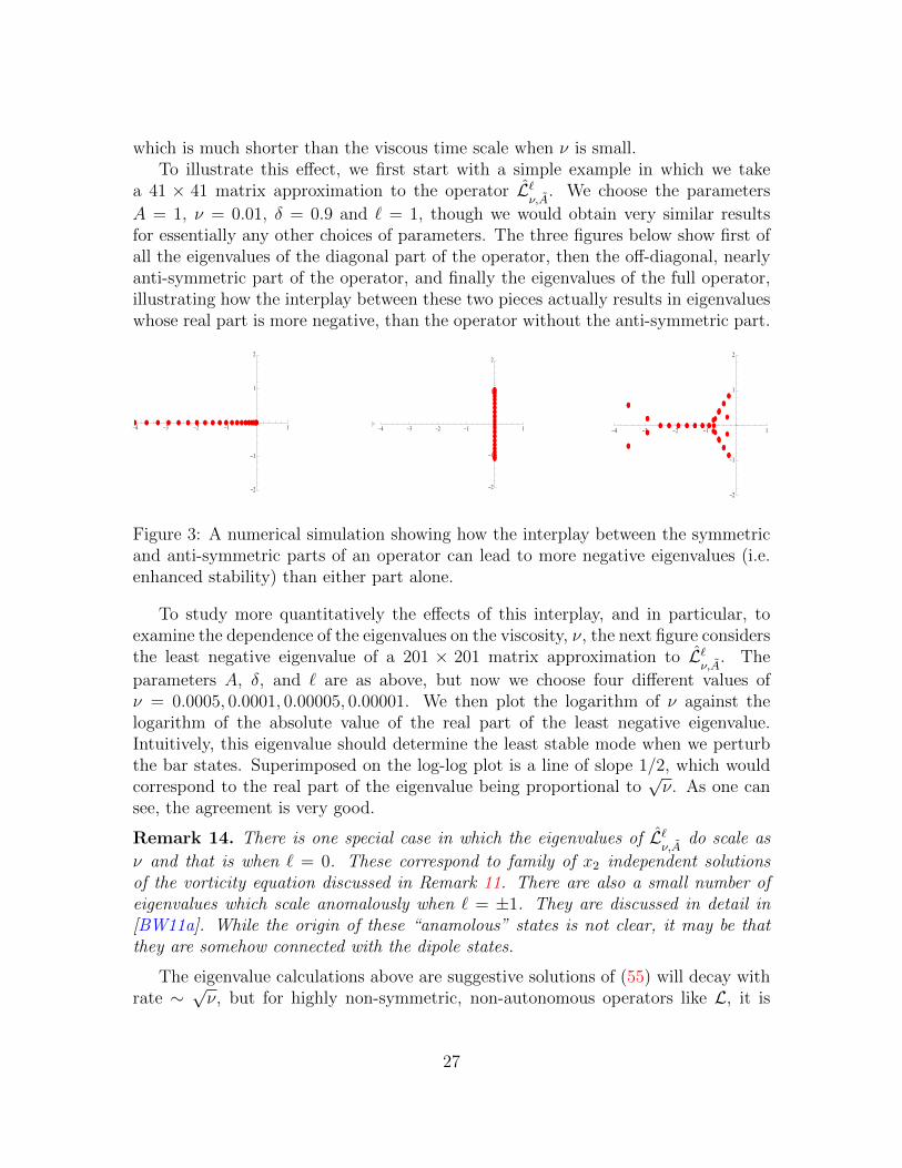
which is much shorter than the viscous time scale when ν is small.To illustrate this effect, we first start with a simple example in which we take

a 41 × 41 matrix approximation to the operator L`ν,A

. We choose the parameters

A = 1, ν = 0.01, δ = 0.9 and ` = 1, though we would obtain very similar resultsfor essentially any other choices of parameters. The three figures below show first ofall the eigenvalues of the diagonal part of the operator, then the off-diagonal, nearlyanti-symmetric part of the operator, and finally the eigenvalues of the full operator,illustrating how the interplay between these two pieces actually results in eigenvalueswhose real part is more negative, than the operator without the anti-symmetric part.

Out[247]=-4 -3 -2 -1 1

-2

-1

1

2

Out[239]=-4 -3 -2 -1 1

-2

-1

1

2

Out[232]=-4 -3 -2 -1 1

-2

-1

1

2

Figure 3: A numerical simulation showing how the interplay between the symmetricand anti-symmetric parts of an operator can lead to more negative eigenvalues (i.e.enhanced stability) than either part alone.

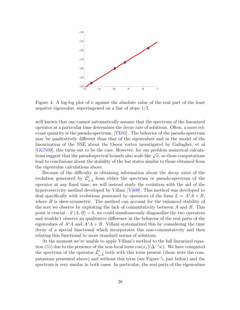
To study more quantitatively the effects of this interplay, and in particular, toexamine the dependence of the eigenvalues on the viscosity, ν, the next figure considersthe least negative eigenvalue of a 201 × 201 matrix approximation to L`

ν,A. The

parameters A, δ, and ` are as above, but now we choose four different values ofν = 0.0005, 0.0001, 0.00005, 0.00001. We then plot the logarithm of ν against thelogarithm of the absolute value of the real part of the least negative eigenvalue.Intuitively, this eigenvalue should determine the least stable mode when we perturbthe bar states. Superimposed on the log-log plot is a line of slope 1/2, which wouldcorrespond to the real part of the eigenvalue being proportional to

√ν. As one can

see, the agreement is very good.

Remark 14. There is one special case in which the eigenvalues of L`ν,A

do scale as

ν and that is when ` = 0. These correspond to family of x2 independent solutionsof the vorticity equation discussed in Remark 11. There are also a small number ofeigenvalues which scale anomalously when ` = ±1. They are discussed in detail in[BW11a]. While the origin of these “anamolous” states is not clear, it may be thatthey are somehow connected with the dipole states.

The eigenvalue calculations above are suggestive solutions of (55) will decay withrate ∼

√ν, but for highly non-symmetric, non-autonomous operators like L, it is

27

Out[302]=

-12 -11 -10 -9 -8 -7-5.0

-4.5

-4.0

-3.5

-3.0

-2.5

-2.0

Figure 4: A log-log plot of ν against the absolute value of the real part of the leastnegative eigenvalue, superimposed on a line of slope 1/2.

well known that one cannot automatically assume that the spectrum of the linearizedoperator at a particular time determines the decay rate of solutions. Often, a more rel-evant quantity is the pseudo-spectrum, [TE05]. The behavior of the pseudo-spectrummay be qualitatively different than that of the eigenvalues and in the model of thelinearization of the NSE about the Oseen vortex investigated by Gallagher, et al[GGN09], this turns out to be the case. However, for our problem numerical calcula-tions suggest that the pseudospectral bounds also scale like

√ν, so these computations

lead to conclusions about the stability of the bar states similar to those obtained fromthe eigenvalue calculations above.

Because of the difficulty in obtaining information about the decay rates of theevolution generated by L`

ν,Afrom either the spectrum or pseudo-spectrum of the

operator at any fixed time, we will instead study the evolution with the aid of thehypercoercivity method developed by Villani [Vil09]. This method was developed todeal specifically with evolutions generated by operators of the form L = A∗A + B,where B is skew-symmetric. The method can account for the enhanced stability ofthe sort we observe by exploiting the lack of commutativity between A and B. Thispoint is crucial – if [A,B] = 0, we could simultaneously diagonalize the two operatorsand wouldn’t observe an qualitative difference in the behavior of the real parts of theeigenvalues of A∗A and A∗A + B. Villani systematized this by considering the timedecay of a special functional which incorporates this non-commutativity and thenrelating this functional to more standard norms of solutions.

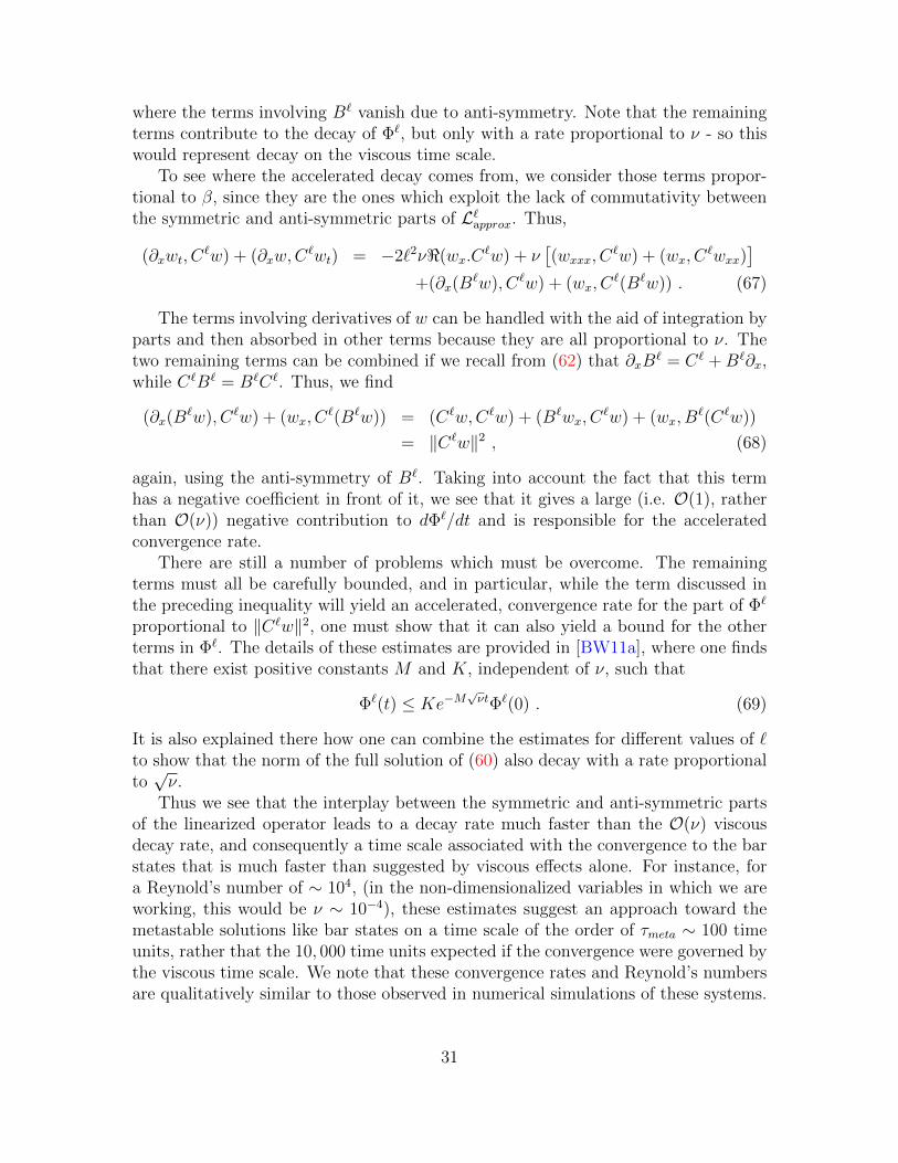
At the moment we’re unable to apply Villani’s method to the full linearized equa-tion (55) due to the presence of the non-local term cos(x1)(∆

−1w). We have computedthe spectrum of the operator L`

ν,Aboth with this term present (those were the com-

putations presented above) and without this term (see Figure 5, just below) and thespectrum is very similar in both cases. In particular, the real parts of the eigenvalues

28

display the same√ν scaling. In addition the non-local term is a compact, lower

order pertrubation so we believe it will have a small influence on the evolution of thesystem. Thus, instead of studying the evolution generated by L`

ν,A, we consider the

approximate equation

∂tw = L`approxw = ν∆w − Ae−νt(cos(x1))∂x2w , (60)

or, if we again expand w in terms of its Fourier series and consider terms with thesame fixed value of `, as we did in (56), we have

∂tw = L`approxw = −ν(∂2x1 − `2)w + i

`

δAe−νt(cos(x1))w . (61)

Out[255]=-4 -3 -2 -1 1

-2

-1

1

2

Figure 5: A plot of the eigenvalues of the approximate linear operator in (60). Theparameter values are the same as in Figure 3

Remark 15. Note that one other advantage of (61) as compared to (54) is that theoperator on the RHS of (61) is already a sum of a symmetric piece plus a skew-symmetric piece, without resorting the initial change of variables needed to bring L`

ν,A

into this form.

Remark 16. In the study of the linearization of the 2D NSE about the Oseen vor-tex a similar nonlocal term appeared in linearization. In [Den12], Deng studied thepseudo-spectrum of the full linearization of the equation and the approximation to thelinearization obtained by dropping the nonlocal term. She found similar results in bothcases.

Remark 17. Note that (61) no longer contains any explicit dependence in x2. Thus,for the remainder of this section we will replace x1 by x to simplify the notation.

29

As mentioned above, Villani’s method exploits the non-commutativity of the sym-metric and skew-symmetric parts of the operator and with that in mind we define thefollowing operators

B`w = i`

δAe−νt(cos(x))w , C`w = [∂x1 , B

`]w = i`

δAe−νt(sin(x))w (62)

Note that like B`, C` is also skew-symmetric, B` and C` commute with each other,and both are bounded operators.

Following Villani, we now define a functional that incorporates the effects of C`

on the evolution, namely,

Φ`(t) = ‖w‖2 + α‖∂xw‖2 − 2β<(∂xw,C`w) + γ(C`wl, C`w). (63)

where the constants α, β, and γ will be chosen in the course of the proof. The firstrestriction we place on their values comes from the fact that we want Φ` to controlsome norm of the solution of (61). If we require that

β2 < αγ/4 , (64)

then we have

‖w‖2 +α

2‖wx‖2 +

γ

2‖C`w‖2 < Φ`(t) < ‖w‖2 +

3α

2‖wx‖2 +

3γ

2‖C`w‖2.

Now consider the time rate of change of the Φ` along a solution of (61). This isalmost identical to the analogous computation in [Vil09], except for minor modifica-tions due to the fact that the operators B` and C` are non-autonomous in our case.Thus, we obtain:

d

dtΦ`(t) = ((wt, w) + (w,wt)) + α ((∂xwt, ∂xw) + (∂xw, ∂xwt)) (65)

−2β<((∂xwt, C

`w) + (∂xw,C`wt)

)+ γ

((C`wt, C

`w) + (C`w,C`wt))

−2β<(∂xw,dC`

dtw) + γ

((dC`

dtw,C`w) + (C`w,

dC`

dtw)

).

We now use (61) and the properties of B` and C` (specifically their anti-symmetry)to control each of the terms in (65). The details of that procedure are set out in[BW11a] – in this review we just focus on a few representative terms, including thosethat give the enhanced stability, to explain the ideas involved.

For instance, consider the terms

(wt, w) + (w,wt) = −ν[(∂2xw,w) + (w, ∂2xw)

]− 2ν`2(w,w)

+(B`w,w) + (w,B`w) (66)

= −2ν[‖w‖2L2 + ‖wx‖2L2

],

30

where the terms involving B` vanish due to anti-symmetry. Note that the remainingterms contribute to the decay of Φ`, but only with a rate proportional to ν - so thiswould represent decay on the viscous time scale.

To see where the accelerated decay comes from, we consider those terms propor-tional to β, since they are the ones which exploit the lack of commutativity betweenthe symmetric and anti-symmetric parts of L`approx. Thus,

(∂xwt, C`w) + (∂xw,C

`wt) = −2`2ν<(wx.C`w) + ν

[(wxxx, C

`w) + (wx, C`wxx)

]+(∂x(B

`w), C`w) + (wx, C`(B`w)) . (67)

The terms involving derivatives of w can be handled with the aid of integration byparts and then absorbed in other terms because they are all proportional to ν. Thetwo remaining terms can be combined if we recall from (62) that ∂xB

` = C` +B`∂x,while C`B` = B`C`. Thus, we find

(∂x(B`w), C`w) + (wx, C

`(B`w)) = (C`w,C`w) + (B`wx, C`w) + (wx, B

`(C`w))

= ‖C`w‖2 , (68)

again, using the anti-symmetry of B`. Taking into account the fact that this termhas a negative coefficient in front of it, we see that it gives a large (i.e. O(1), ratherthan O(ν)) negative contribution to dΦ`/dt and is responsible for the acceleratedconvergence rate.

There are still a number of problems which must be overcome. The remainingterms must all be carefully bounded, and in particular, while the term discussed inthe preceding inequality will yield an accelerated, convergence rate for the part of Φ`

proportional to ‖C`w‖2, one must show that it can also yield a bound for the otherterms in Φ`. The details of these estimates are provided in [BW11a], where one findsthat there exist positive constants M and K, independent of ν, such that

Φ`(t) ≤ Ke−M√νtΦ`(0) . (69)

It is also explained there how one can combine the estimates for different values of `to show that the norm of the full solution of (60) also decay with a rate proportionalto√ν.

Thus we see that the interplay between the symmetric and anti-symmetric partsof the linearized operator leads to a decay rate much faster than the O(ν) viscousdecay rate, and consequently a time scale associated with the convergence to the barstates that is much faster than suggested by viscous effects alone. For instance, fora Reynold’s number of ∼ 104, (in the non-dimensionalized variables in which we areworking, this would be ν ∼ 10−4), these estimates suggest an approach toward themetastable solutions like bar states on a time scale of the order of τmeta ∼ 100 timeunits, rather that the 10, 000 time units expected if the convergence were governed bythe viscous time scale. We note that these convergence rates and Reynold’s numbersare qualitatively similar to those observed in numerical simulations of these systems.

31

Of course the picture in the case of metastable behavior for the 2D NSE is still farless complete than for Burgers equation. The most important missing piece is the factthat so far, the rigorous estimates only apply to the approximation of the true linearevolution obtained by dropping the nonlocal term in the equation. However, as wehave seen from the numerical computations presented above, the spectral propertiesof the operator with or without the nonlocal term are very similar, and we hope thatthe sort of techniques Deng developed in [Den11] will also apply here and allow us totreat the full linearized operator.

A second important difference between Burgers equation and the 2D NSE is thatin Burgers equation the viscous N-waves are the only metastable states for almostall solutions, but for the NSE there are other candidates, such as the dipole statesobserved in numerics (see Remark 12), or the states discussed in Remark 11 whichlike the bar states only depend on one of the two spatial variables. This means thatthe final picture of metastability for the NSE will undoubtedly be more complicatedthan the simple picture in Figure 2 for Burgers equation. Nonetheless, we feel thatthese dynamical systems ideas can yield important simplifying insights into the in-termediate asymptotics of this important physical system and can explain how timescales much shorter than the viscous time scales can arise from the operators whichhave a small, symmetric dissipative piece, and a large, anti-symmetric component,which arise frequently in the study of fluid motions.

4 Finite Dimensional Attractors for the Navier-

Stokes equations

In the two previous sections we focussed on the behavior of the two-dimensionalNavier-Stokes equations in the absence of forcing and studied the types of structuresthat emerged on intermediate and long time scales. In the present section we considersolutions of the equation when it is subjected to external forcing. In practice, suchforcing might arise through shearing at the boundaries of the domain, as is the casein the Taylor-Couette experiment, but as is often done in theoretical studies we willallow for a general body force, i.e. we will consider the form of the equations in (10)and (11).

∂tu + u · ∇u = ν∆u−∇p+ g (70)

∇ · u = 0 . (71)

Here the forcing term g is some general vector valued function whose smoothness wespecify below.

Numerical studies show that even in the presence of certain types of forcing,the structures we studied in previous sections may still play a dominant role in thedynamical behavior of the system [BS09]. However, in this section we focus on moregeneral properties of the system such as the existence and dimension of the attractor

32

for the system. We will present fewer details of the calculations in this section thanin the prior ones since the work described here is somewhat older than that in theprevious sections and several excellent monograph length reviews of these resultsalready exist [Rob01], [DG95].

While most investigations of these questions work directly with the fluid velocity,in order to keep the discussion as close as possible to prior sections we will continue towork with the vorticity formulation of the problem. This has the disadvantage thatwe are restricted essentially to domains without boundary and thus we focus here asin section three on a rectangular domain with periodic boundary conditions, so weconsider functions in

L2(T2δ) = uj ∈ L2 | uj(x1, x2) = uj(x1 +2π, x2) = uj(x1, x2 +2πδ) , j = 1, 2 . (72)

Assuming that the forcing g is differentiable, we can then take the curl of (70) toobtain the scalar equation

∂tω = ν∆ω − u · ∇ω + f , (73)

where u is again the velocity field recovered from the vorticity via the Biot-Savartlaw (47), and f = ∂x1g2 − ∂x2g1.

Proving the existence and uniqueness of solutions for this equation is straightfor-ward so we will assume that has been done and focus instead on more detailed aspectsof its dynamics. Recall from the introduction that an infinite dimensional dynamicalsystem is dissipative if the phase space contains a precompact absorbing ball. Thatfollows in the present circumstances from straightforward energy estimates. If wemultiply (73) by ω and integrate over the torus, we find that

∂t‖ω(t)‖L2 = −ν‖∇ω‖2L2 −∫T2δ

ω(u · ∇ω)dx+

∫T2δ

ωfdx . (74)

Consider each of the terms on the RHS of this equation in turn. Since∫ωdx = 0, we

can apply Poincare’s inequality to the first term and bound it by −cpν‖ω‖2L2 . Turningto the second term, the incompressibility of the velocity field u allows us to rewriteit as: ∫

T2δ

ω(u · ∇ω)dx =1

2

∫T2δ

u · ∇ω2dx =1

2

∫T2δ

∇ · (uω2)dx = 0 , (75)

where the last inequality follows from the periodic boundary conditions. Finally theCauchy-Schwartz inequality implies that |

∫ωfdx| ≤ ‖ω‖L2‖f‖L2 ≤ 1

2cpν‖ω‖2L2 +

12cpν‖f‖2L2 . Inserting these estimates into (74) we find

∂t‖ω(t)‖L2 = −1

2cpν‖ω‖2L2 +

1

2cpν‖f‖2L2 . (76)

33

If we now assume that the forcing function is an element of L∞([0,∞);L2(T2δ)), we

can apply Gronwall’s inequality to conclude that

‖ω(t)‖2L2 ≤ e−cpνt/2‖ω0‖2L2 +2

cpν(1− e−cpνt/2)‖f‖L∞([0,∞);L2) . (77)

and so we see that all solutions of (73) will eventually enter the ball of radius R =2cpν‖f‖L∞([0,∞);L2).

As noted in the introduction, in infinite dimensional systems, the existence ofan absorbing ball is not enough in itself to guarantee an attractor. We much showthat the absorbing set is also (pre-)compact in L2. One does this by showing theboundedness of the absorbing ball in Hs, with s ≥ 1, and using the fact that Hs

is compactly embedded in L2. The boundedness of the Hs norm follows by energyestimates similar to those in (74)-(76). They are somewhat more complicated in thiscase though because the nonlinear term no longer vanishes as in (75). One still obtainsa bound on the Hs norm though and as a consequence the existence of a bounded,compact attractor for the forced two-dimensional NSE. In fact, in two-dimensions,there is a whole sequence of energy estimates linking and bounding the various Sobelevnorms of the solution - for an explication of these estimates, sometimes known as theladder theorems, see [DG95].

As discussed in the introduction, one advantage of the existence of an attractor isthat it often allows one to focus attention on a much smaller dimensional system thanthe original, infinite dimensional PDE. In fact, the attractor for the two-dimensionalNSE is finite dimensional and one can estimate its dimension in terms of the forcingfunction f . This fact was first established for a class of reaction-diffusion equationsby Mallet-Paret [MP76]. In the context of the two-dimensional NSE is first studiedby Constantin and Foias, [CF85]. It is well known that the attractor of a chaoticdynamical system is often a fractal set and so to measure it, we must use a fractaldimension. There are several common fractal dimensions including the Hausdorffdimensional and the capacity dimension. Estimates of the both these quantitiesexist in the case of the attractor in the two-dimensional NSE, but we’ll focus on thecapacity here because it is the simplest to define. Given a set A in the phase-space ofour PDE, define N(r) = min number of balls of radius r needed to cover A. Thenthe capacity dimension of A is defined to be:

dC(A) = lim supr→0

N(r)

log(1/r). (78)

It is easy to check that if one takes a segment of a curve or surface in Rd, the ca-pacity dimension gives the usual and expected values of 1 and 2 respectively. Supposenow that we consider the attractor for the two-dimensional NSE. The basic idea relat-ing the dimensional estimates to the dynamics of the system is the following. Supposeone covers the attractor with d-dimensional balls of radius r. On can show that ifthe attractor is finite dimensional it suffices to use finite (although perhaps large)

34

dimensional balls to compute the dimension. If one considers how these balls willbe distorted by the flow, say by the time-one map of the system, they will typicallybe elongated in some directions, corresponding to the chaotic stretching that occursin the attractor. However, the high-frequency modes in the Navier-Stokes equationare very strongly damped, and if we choose d, the dimension of the covering balls,sufficiently large, the number of contracting directions will overwhelm the effect ofthe expanding directions and result in the total volume of the ball shrinking. Thecapacity is defined in terms of the limit as the radius of the balls tends to zero sowe are most interested in the action of the flow on balls of very small radius. In thislimit, the action of the flow is well approximated by the linearization of the flow,which will distort our original ball into a d-dimensional ellipsoid. The lengths of theaxes of this ellipsoid can then be related to the radius of the original ball by thesingular values of the linearized system, which are in turn related to the Lyapunovexponents of the dynamical system. If the Lyapunov exponents of the system areµ1 ≥ µ2 ≥ . . . , (where we have listed the exponents along with their multiplicity),then the shortest axis of the deformed ellipsoid should have length ∼ reµd , and thevolume on the ellipsoid should be approximately ∼ rdeµ1+...µd . This in turn gives arecursion relation between N(r) and N(eµd), which can then be used to evaluate thelim sup in (78). The details of this calculation are very clearly explained in( [DG95],p. 67) and lead to an estimate of the dimension in terms of the attractor. 1

There are a number of points that must be addressed in order to make this argu-ment rigorous including:

• The Lyapunov exponents concern the asymptotic growth rates of the linearizedflow, not the amount of growth or shrinking that occurs in the time-one map.

• Typically, the Lyapunov exponents will depend on the initial point we choose,so it’s not clear why this argument leads to a uniform estimate on the dimensionof the attractor.

• Finally, we would like to have an estimate on the attractor dimension in termsof accessible quantities in the equation, like the viscosity, ν, or the forcing f ,rather than generally unknown Lyapunov exponents.

Constantin and Foias address the first two points by introducing global Lyapunovexponents. They consider the usual definition of the Lyapunov exponents in terms ofthe growth rates of n-dimensional volumes induced by the linearized flow, but beforetaking the infinite time limit of these growth rates, they take the supremum of thegrowth rates over the attractor. This gives an estimate of the growth rate independentof the starting point, but might lead to an overestimate of the dimension. They alsogive rigorous estimates relating the size of a ball of radius r, transported for a finite

1The link between the attractor dimension and the Lyapunov exponents was first proposed byKaplan and Yorke, [KY79], and is often known as the Kaplan-Yorke formula.

35

time t, to these global Lyapunov exponents, as well of making rigorous the details ofthe Kaplan-Yorke formula for infinite dimensional systems like the NSE.

To relate the Lyapunov exponents of the NSE to the quantities that appear in theequation, note that if we linearize (73) about a solution ω(t), with associated velocityfield u(t), the linearized equation takes the form:

∂tW = ν∆W − u · ∇W −U · ∇ω , (79)

where U is the velocity field associated with W .Recall that the estimates of dimension were based on how the linearized flow causes

d-dimensional spheres to expand or contract. Thus, instead of studying (79) directly,we consider the evolution of (PdW ), the projection of W onto an d-dimensional sub-space of the infinite dimensional phase space, and consider the maximum growth rateover all such projections. The growth rate of such projections can be controlled byenergy estimates of the type that lead to (77), and one finds

dC ≤ C

(‖g‖L2

ν2

)2/3(1 + log

(4π2δ

ν2‖g‖L2

)). (80)

In this estimate, the factor of 4π2δ is just the area of the domain on which theequation evolves, and g is the forcing term in the equation for the velocity field, notthe vorticity, and this force is assumed to be constant in time. Note that althoughthe forcing function for the fluid velocity appears in the estimate of dimension, theactual estimates are done in the vorticity formulation which seems to yield sharperbounds on the attractor dimension than working directly with the vorticity [CFT88].For more details on the derivation of these estimates, one can consult either theoriginal paper, [CF85], which explains the ideas behind the proof very clearly, or themonograph, [DG95].

Remark 18. There is a non-rigorous estimate of the dimension of the attractorof the two-dimensional Navier-Stoke equation based on a scaling theory of turbulence.Remarkably, the rigorous estimate (80) agrees with the prediction of the scaling theory,

up to the factor of(

1 + log(

4π2δν2‖g‖L2

)).

Remark 19. Bounding the dimension of the attractor is one way to quantify theessentially finite dimensional nature of the two-dimensional NSE semi-flow. Anotherapproach focuses on showing that there is a finite number of determining modes ordetermining nodes. In this case, one asks whether or not the knowledge of the behaviorof the projection of the solution on a finite number of modes, or its value at a finitenumber of points, is sufficient to determine its long time behavior. More precisely, letPd be the projection onto an d-dimensional subspace discussed above. One says thatthe system has d determining modes if for some choice of Pd, any two solutions ω(t)and ω(t) for which

limt→∞‖Pd(ω(t))− Pd(ω(t))‖L2 = 0 , (81)

36

must also havelimt→∞‖ω(t)− ω(t)‖L2 = 0 , (82)

with a similar definition for determining nodes. Note that this definition does notimply that given a knowledge of the first d modes of the system we can reconstruct theremaining modes, but merely that those (infinitely many) other modes cannot changethe long-term asymptotics of the solution.

The first estimates establishing that the solutions of the two-dimensional NSE hada finite number of determining modes were by Foias and Prodi [FP67]. More recently,Jones and Titi, [JT93] have shown that the for periodic boundary conditions, thenumber of determining modes is bounded by

d ≤ C‖g‖L2

ν2, (83)

which is larger than estimate for the dimension of the attractor established above.

While the finite dimensionality of the attractor for the two-dimensional NSE im-plies that the asymptotic behavior is determined by the motions on some “small”piece of the phase space, it doesn’t immediately imply that there is a smooth finitedimensional dynamical system whose motion reproduces the long-time behavior ofthe NSE. The reason is that one knows very little about the structure of the attractorand in fact, for chaotic systems, it is expected to be a complicated, fractal set. Thus,simply restricting the NSE to the attractor will not generally lead to a smooth, finitedimensional, dynamical system. An alternate approach which has been pursued is toattempt to construct a finite dimensional manifold which is:

• smooth, or at least Lipshitz,

• invariant with respect to the semi-flow defined by the NSE, and

• attracts any solution of the equation at an exponential rate.

Such manifolds, if they exist, are called inertial manifolds.If a PDE possesses an inertial manifold, then by its invariance and attractivity, the

attractor must lie inside it. Thus, by restricting the PDE to the inertial manifold oneobtains a smooth (or at least Lipshitz), finite dimensional dynamical system whichcaptures all the asymptotic behavior of the original, infinite dimensional system.

Inertial manifolds bear much resemblance to center manifolds in finite dimensionalsystems of ordinary differential equations. Recall that the existence theory for centermanifolds requires that the “spectral gap”, that is, the difference between the realparts of the stable and unstable eigenvalues and the center eigenvalues, must be largein comparison with the Lipschitz constant of the nonlinear term in the equation.

In the inertial manifold case, this becomes the requirement that there be a largegap between the eigenvalues corresponding to modes related to the inertial manifold

37

and those “off” the manifold. Typically the distinction between these two sets ofmodes is expressed by writing the inertial manifold is written as a graph of a functionwhose domain is the span of the first set of these modes and whose range is the spanof the modes off the manifold. The size of the gap is again related to the propertiesof the nonlinear term, but are more complicated than those in the ODE case becausethe nonlinear term in the PDE is often not Lipshitz on the whole phase space ofthe system. For example, consider the nonlinear term in the vorticity equation (73).The presence of the derivative in the nonlinearity means it is not even defined on thewhole phase space, L2(T2

δ), let alone Lipschitz. This lack of smoothness results inmuch more stringent spectral conditions than in the center manifold case.

For nonlinear terms of the sort that appear in the NSE, the best estimates to datefor the spectral gap require that if the eigenvalues of the linear part of the equationare ordered as 0 ≥ −λ1 ≥ −λ2 ≥ . . . , then proof of existence for the inertial manifoldrequires that for a manifold on dimension N , one must have:

λN+1 − λN ≥ K(λ1/2N+1 + λ

1/2N ) . (84)

For (73), the eigenvalues of the linear part can be explicitly computed as ν(m2+(`/δ)2,and one sees that the large gaps required by (84) do not exist. As a consequence, thereis no proof to date, that the two-dimensional NSE possesses an inertial manifold.

There are, however, large classes of dissipative PDEs for which the existence ofan inertial manifold has been proven. Most of these fall into one of two categories:

1. 1-dimensional equations: In one dimension, if one considers a PDE with linearpart

∂tu = ν∂rxu , (85)

with periodic boundaries on the interval [−π, π], the eigenvalues are −λn =−νn2r. Thus, for r > 1/2, one obtains arbitrarily large gaps between eigenvaluesas n grows. Using this growth, the existence of inertial manifolds for equationslike the Kuramoto-Sivishinsky and Cahn-Hilliard, [FST85], [FST88], [CFNT89].

2. Equations with “nicer” nonlinear terms: If the nonlinear term in the equationis a smooth function on the phase space of the equation, as is true for manyreaction-diffusion equations, the spectral gap condition can be greatly weakenedand the existence of inertial manifolds for many two-dimensional domains, andeven some special three-dimensional domains has been established, [MPS88].

In conclusion, we have seen that the tools of dynamical systems theory providea number of insights into the qualitative behavior of solutions of dissipative PDEs,especially the two-dimensional Navier-Stokes equations. The identification of finitedimensional invariant structures in the infinite dimensional phase space of these sys-tems, be they attractors, or invariant manifolds, allow one to better understand the

38

long-time asymptotic behavior of both the forced and unforced Navier-Stokes equa-tions, as well as providing a way of understanding the emergence of intermediate timescales in these systems.

Acknowledgements: This research is supported in part by the National ScienceFoundation, DMS-0908093. For those parts of this survey which describe my ownresearch it is a pleasure to thank my collaborators - Thierry Gallay and MargaretBeck for the theoretical results in Sections 2 and 3, and Alethea Barbaro, Ray Nagem,Guido Sandri and David Uminsky for the numerical methods described in Section 2.

References

[BA94] Matania Ben-Artzi. Global solutions of two-dimensional Navier-Stokesand Euler equations. Arch. Rational Mech. Anal., 128(4):329–358, 1994.

[BJ89] Peter W. Bates and Christopher K. R. T. Jones. Invariant manifoldsfor semilinear partial differential equations. In Dynamics reported, Vol.2, volume 2 of Dynam. Report. Ser. Dynam. Systems Appl., pages 1–38.Wiley, Chichester, 1989.

[BS09] Freddy Bouchet and E. Simonnet. Random changes of flow topol-ogy in two-dimensional and geophysical turbulence. Phys. Rev. Lett.,102(094504), 2009.

[BW11a] Margaret Beck and C. Eugene Wayne. Metastability and rapid conver-gence to quasi-stationary bar states for the 2D Navier-Stokes equations.Preprint; arXiv:1108.3416; to appear in Proc. Roy. Soc. Edin., 2011.

[BW11b] Margaret Beck and C. Eugene Wayne. Using global invariant manifoldsto understand metastability in the Burgers equation with small viscosity.SIAM Review, 53(1):129–153 [Expanded and revised version of paper ofthe same title published originally in SIAM J. Appl. Dyn. Syst. 8 (2009),no. 3, 1043–1065], 2011.

[CF85] P. Constantin and C. Foias. Global Lyapunov exponents, Kaplan-Yorkeformulas and the dimension of the attractors for 2D Navier-Stokes equa-tions. Comm. Pure Appl. Math., 38(1):1–27, 1985.

[CFNT89] P. Constantin, C. Foias, B. Nicolaenko, and R. Temam. Integral mani-folds and inertial manifolds for dissipative partial differential equations,volume 70 of Applied Mathematical Sciences. Springer-Verlag, New York,1989.

[CFT88] P. Constantin, C. Foias, and R. Temam. On the dimension of the attrac-tors in two-dimensional turbulence. Phys. D, 30(3):284–296, 1988.

39

[CHT97] Xu-Yan Chen, Jack K. Hale, and Bin Tan. Invariant foliations for C1

semigroups in Banach spaces. J. Differential Equations, 139(2):283–318,1997.

[CL95] Eric A. Carlen and Michael Loss. Optimal smoothing and decay estimatesfor viscously damped conservation laws, with applications to the 2-DNavier-Stokes equation. Duke Math. J., 81(1):135–157 (1996), 1995. Acelebration of John F. Nash, Jr.

[Den11] Wen Deng. Pseudospectrum for Oseen vortices operators. Preprint;arXiv:1109.4798 [math.AP], 2011.

[Den12] Wen Deng. Etude du pseudo-spectre d’operateurs non auto-adjoints liesa la mecanique des fluides. PhD thesis, Universite Pierre et Marie Curie,2012.

[DG95] Charles R. Doering and J. D. Gibbon. Applied analysis of the Navier-Stokes equations. Cambridge Texts in Applied Mathematics. CambridgeUniversity Press, Cambridge, 1995.

[FP67] C. Foias and G. Prodi. Sur le comportement global des solutions non-stationnaires des equations de Navier-Stokes en dimension 2. Rend. Sem.Mat. Univ. Padova, 39:1–34, 1967.

[FST85] Ciprian Foias, George R. Sell, and Roger Temam. Varietes inertielles desequations differentielles dissipatives. C. R. Acad. Sci. Paris Ser. I Math.,301(5):139–141, 1985.

[FST88] Ciprian Foias, George R. Sell, and Roger Temam. Inertial manifolds fornonlinear evolutionary equations. J. Differential Equations, 73(2):309–353, 1988.

[GG05] Isabelle Gallagher and Thierry Gallay. Uniqueness for the two-dimensional Navier-Stokes equation with a measure as initial vorticity.Math. Ann., 332(2):287–327, 2005.

[GGN09] Isabelle Gallagher, Thierry Gallay, and Francis Nier. Special asymptoticsfor large skew-symmetric perturbations of the harmonic oscillator. Int.Math. Res. Not. IMRN, (12):2147–2199, 2009.

[GMO88] Yoshikazu Giga, Tetsuro Miyakawa, and Hirofumi Osada. Two-dimensional Navier-Stokes flow with measures as initial vorticity. Arch.Rational Mech. Anal., 104(3):223–250, 1988.

[GW02] Thierry Gallay and C. Eugene Wayne. Invariant manifolds and the long-time asymptotics of the Navier-Stokes and vorticity equations on R2.Arch. Ration. Mech. Anal., 163(3):209–258, 2002.

40

[GW05] Thierry Gallay and C. Eugene Wayne. Global stability of vortex so-lutions of the two-dimensional Navier-Stokes equation. Comm. Math.Phys., 255(1):97–129, 2005.

[Hal88] Jack K. Hale. Asymptotic behavior of dissipative systems, volume 25 ofMathematical Surveys and Monographs. American Mathematical Society,Providence, RI, 1988.

[Hen81] Daniel Henry. Geometric theory of semilinear parabolic equations, volume840 of Lecture Notes in Mathematics. Springer-Verlag, Berlin, 1981.

[JT93] Don A. Jones and Edriss S. Titi. Upper bounds on the number of deter-mining modes, nodes, and volume elements for the Navier-Stokes equa-tions. Indiana Univ. Math. J., 42(3):875–887, 1993.

[KT01] Y.-J. Kim and A. E. Tzavaras. Diffusive N -waves and metastability inthe Burgers equation. SIAM J. Math. Anal., 33(3):607–633 (electronic),2001.

[KY79] James Kaplan and James Yorke. Chaotic behavior of multidimensionaldifference equations. In Heinz-Otto Peitgen and Hans-Otto Walther,editors, Functional Differential Equations and Approximation of FixedPoints, volume 730 of Lecture Notes in Mathematics, pages 204–227.Springer Berlin / Heidelberg, 1979. 10.1007/BFb0064319.

[LL97] Elliott H. Lieb and Michael Loss. Analysis, volume 14 of Graduate Studiesin Mathematics. American Mathematical Society, Providence, RI, 1997.

[Mie91] Alexander Mielke. Locally invariant manifolds for quasilinear parabolicequations. Rocky Mountain J. Math., 21(2):707–714, 1991. Current di-rections in nonlinear partial differential equations (Provo, UT, 1987).

[Mik98] Milan Miklavcic. Applied functional analysis and partial differential equa-tions. World Scientific Publishing Co. Inc., River Edge, NJ, 1998.

[MP76] John Mallet-Paret. Negatively invariant sets of compact maps and an ex-tension of a theorem of Cartwright. J. Differential Equations, 22(2):331–348, 1976.

[MPS88] John Mallet-Paret and George R. Sell. Inertial manifolds for reactiondiffusion equations in higher space dimensions. J. Amer. Math. Soc.,1(4):805–866, 1988.

[MS01] Tetsuro Miyakawa and Maria Elena Schonbek. On optimal decay ratesfor weak solutions to the Navier-Stokes equations in Rn. In Proceedings ofPartial Differential Equations and Applications (Olomouc, 1999), volume126, pages 443–455, 2001.

41

[NSUW09] Raymond Nagem, Guido Sandri, David Uminsky, and C. Eugene Wayne.Generalized Helmholtz-Kirchhoff model for two-dimensional distributedvortex motion. SIAM J. Appl. Dyn. Syst., 8(1):160–179, 2009.

[PP95] A. Prochazka and D. I. Pullin. On the two-dimensional stability of theaxisymmetric Burgers vortex. Phys. Fluids, 7(7):1788–1790, 1995.

[Rob01] James C. Robinson. Infinite-dimensional dynamical systems. CambridgeTexts in Applied Mathematics. Cambridge University Press, Cambridge,2001. An introduction to dissipative parabolic PDEs and the theory ofglobal attractors.

[TE05] Lloyd N. Trefethen and Mark Embree. Spectra and pseudospectra. Prince-ton University Press, Princeton, NJ, 2005. The behavior of nonnormalmatrices and operators.

[Tem88] Roger Temam. Infinite-dimensional dynamical systems in mechanics andphysics, volume 68 of Applied Mathematical Sciences. Springer-Verlag,New York, 1988.

[UEWB12] David Uminsky, C. Eugene Wayne, and Alethea Barbaro. A multi-moment vortex method for 2D viscous fluids. J. Comput. Phys.,231(4):1705–1727, 2012.

[VI92] A. Vanderbauwhede and G. Iooss. Center manifold theory in infinitedimensions. In Dynamics reported: expositions in dynamical systems,volume 1 of Dynam. Report. Expositions Dynam. Systems (N.S.), pages125–163. Springer, Berlin, 1992.

[Vil09] Cedric Villani. Hypocoercivity. Mem. Amer. Math. Soc.,202(950):iv+141, 2009.

[Way11] C. Eugene Wayne. Vortices and two-dimensional fluid motion. NoticesAmer. Math. Soc., 58(1):10–19, 2011.

[YMC03] Z. Yin, D. C. Montgomery, and H. J. H. Clercx. Alternative statistical-mechanical descriptions of decaying two-dimensional turbulence in termsof “patches” and “points”. Phys. Fluids, 15:1937–1953, 2003.

42