DISCUSSION PAPER SERIES

IZA DP No. 12632

Steffen KünnJuan PalaciosNico Pestel

Indoor Air Quality and Cognitive Performance

SEPTEMBER 2019

Any opinions expressed in this paper are those of the author(s) and not those of IZA. Research published in this series may include views on policy, but IZA takes no institutional policy positions. The IZA research network is committed to the IZA Guiding Principles of Research Integrity.The IZA Institute of Labor Economics is an independent economic research institute that conducts research in labor economics and offers evidence-based policy advice on labor market issues. Supported by the Deutsche Post Foundation, IZA runs the world’s largest network of economists, whose research aims to provide answers to the global labor market challenges of our time. Our key objective is to build bridges between academic research, policymakers and society.IZA Discussion Papers often represent preliminary work and are circulated to encourage discussion. Citation of such a paper should account for its provisional character. A revised version may be available directly from the author.

Schaumburg-Lippe-Straße 5–953113 Bonn, Germany

Phone: +49-228-3894-0Email: publications@iza.org www.iza.org

IZA – Institute of Labor Economics

DISCUSSION PAPER SERIES

ISSN: 2365-9793

IZA DP No. 12632

Indoor Air Quality and Cognitive Performance

SEPTEMBER 2019

Steffen KünnMaastricht University, ROA and IZA

Juan PalaciosMassachusetts Institute of Technology and IZA

Nico PestelIZA

ABSTRACT

IZA DP No. 12632 SEPTEMBER 2019

Indoor Air Quality and Cognitive Performance*

This paper studies the causal impact of indoor air quality on the cognitive performance

of individuals using data from official chess tournaments. We use a chess engine to

evaluate the quality of moves made by individual players and merge this information

with measures of air quality inside the tournament venue. The results show that poor

indoor air quality hampers cognitive performance significantly. We find that an increase

in the indoor concentration of fine particulate matter (PM2.5) by 10 μg/m3 increases a

player’s probability of making an erroneous move by 26.3%. The impact increases in both

magnitude and statistical significance with rising time pressure. The effect of the indoor

concentration of carbon dioxide (CO2) is smaller and only matters during phases of the

game when decisions are taken under high time stress. Exploiting temporal as well as

spatial variation in outdoor pollution, we provide evidence suggesting a short-term and

transitory effect of fine particulate matter on cognition.

JEL Classification: D91, I1, J24, Q50, Z20

Keywords: indoor air quality, cognition, worker productivity, chess

Corresponding author:Steffen KünnMaastricht UniversitySchool of Business and EconomicsDepartment of EconomicsTongersestraat 536211 LM MaastrichtThe Netherlands

E-mail: s.kuenn@maastrichtuniversity.nl

* The authors thank Thomas Dohmen, Matthew Neidell, Joshua Graff Zivin, Michael Greenstone, Piet Eichholtz,

Nils Kok, and Christian Seel, as well as seminar participants at IZA Bonn, Maastricht University, the 2019 annual

meetings of the European Association of Labour Economists and the European Society of Population Economics for

their helpful comments and suggestions. Rafael Suchy, Sergej Bechtoldt and Nicolas Meys provided excellent research

assistance in collecting the data. We gratefully acknowledge the financial support by the Graduate School of Business

and Economics at Maastricht University as well as IZA Bonn.

1 Introduction

Environmental pollution is estimated to be responsible for nine million premature deaths an-

nually (Landrigan et al., 2018). While most countries impose strict regulations on the emission

of air pollutants to improve ambient air quality, the current calculations of societal cost of air

pollution may be substantially underestimated as a growing body of evidence in health sciences

suggests that exposure to poor air quality may also have harmful immediate and lasting impacts

on the human brain, ultimately lowering individuals’ cognitive abilities (Underwood, 2017). Ex-

posure to air pollution alone has been shown to have severe health consequences which may

translate into adverse effects on human capital formation and labor market outcomes in the

short and long run (Graff Zivin and Neidell, 2013, 2018).1 These physiological effects on human

cognition may have severe consequences for individual performance in complex cognitive tasks.

This paper examines the causal impact of indoor air quality on the cognitive performance

of individuals using data from chess tournaments. Chess provides an ideal setting to study the

relationship between environmental conditions and individuals’ cognition. Chess is a complex

and cognitively demanding activity (Vaci et al., 2019), where individuals face strong incentives

to exert high effort and which involves strategic decision making under time pressure. The

quality of cognitive performance can be objectively evaluated at high frequency using a chess

engine as a benchmark. In addition, our study uses measures of air quality from inside the room

where individuals are executing the tasks, which provides unambiguous information on players’

exposure to environmental conditions.

We use a unique panel dataset on the performance of chess players obtained from tournaments

held in Germany in 2017, 2018 and 2019. The data contain detailed information on about 30,000

moves made by 121 players in 596 games. Each tournament edition comprises seven rounds over

a period of eight weeks, which provides us with sufficient natural variation in indoor air quality.

Players’ skills range from beginner to advanced levels. All players have strong incentives to

perform well throughout the tournament as the outcomes in each game count for their official

chess rating score, which is a matter of prestige among chess players and has implications for

future competitions. In addition, monetary prizes provide pecuniary incentives. We make use

of a state of the art chess engine to measure the quality of players’ decisions. The chess engine

evaluates actual moves made by the players and compares them to moves deemed optimal

according to its algorithm. Based on the engine’s output we construct two outcome variables:

(i) a binary indicator for moves annotated as an error and (ii) the magnitude of the error.1Air pollution increases direct medical costs, such as hospitalizations and pharmaceutical expenses (Schlenker

and Walker, 2016; Deschenes et al., 2017). Further, students perform worse in high-stakes examinations (Ebensteinet al., 2016) and workers spent less time on the job when ambient air pollution is higher (Hanna and Oliva, 2015;Aragon et al., 2017). Similarly, extremely warm days lead to a reduction in working hours (Graff Zivin and Neidell,2014).

1

Our identification strategy exploits the panel structure of the data. We observe the perfor-

mance of the same individuals playing multiple games against different opponents in the exact

same venue, at the same time of the day, but under varying levels of indoor air quality which are

beyond the control of the players. In order to accurately assign players’ exposure to air quality,

we installed sensors inside the tournament venue continuously measuring indoor environmental

conditions. We focus on the concentration of fine particulate matter with a diameter smaller

than 2.5 micrometers (PM2.5), which may penetrate deep into the lungs and brains. Evidence

from epidemiology and toxicology suggests that exposure to air pollution can hinder cognition

by causing inflammatory reactions (Underwood, 2017; Kumar, 2018) and by reducing the trans-

portation of oxygen to the brain (Bernstein et al., 2004). In addition to particulate pollution,

we study potential effects of variation in the concentration of carbon dioxide (CO2). High levels

of CO2 have been linked to dizziness, headache or fatigue (Stankovic et al., 2016). In addition,

we control for other environmental conditions such as temperature, humidity and noise.

Overall, our results show that indoor concentration of fine particles significantly deteriorates

cognitive performance. Exploiting within-player variation in air quality and controlling for year,

round, and move fixed effects, and a set of control variables including other environmental

conditions, we find that an increase in fine particulate pollution (PM2.5) of ten micrograms per

cubic meter (10 µg/m3), about three quarters of a standard deviation in the sample, leads to a

2.1 percentage point increase in the probability of making a meaningful error. This corresponds

to an increase by 26.3% relative to the sample mean. We do not find evidence for effects of the

observed variation in carbon dioxide in the full sample of moves.

In addition, the high frequency of our performance measures allows to examine effect hetero-

geneity with respect to time pressure as the tournament rules set a time restriction. In all games

in our sample, each player has to complete the first 40 moves within a time limit of 110 minutes.

This implies that, when approaching move 40, move decisions can be assumed to be made under

relative time pressure, compared to other phases of the game. The impact of PM2.5 increases

in both magnitude and statistical significance with increasing time pressure, with the most pro-

nounced effect shortly before move 40. In contrast, the effect of CO2 is smaller in magnitude

and is only statistically significant just before the time control is applied. This suggests that

poor air quality harms the performance of players particularly if acting under time pressure.

Moreover, we find older individuals’ performance being more sensitive to poor air quality, and

an increased effect of pollution if players are faced with a stronger opponent, which may be in

itself a more stressful situation.

Finally, we explore the role of outdoor pollution in shaping indoor conditions. The variation

in indoor particulate pollution largely reflects levels of air pollution in the (outdoor) vicinity

of the tournament site, coming from automobile exhaust or industrial emissions. Using out-

2

door pollution measures stemming from nearby air quality stations, we find very similar results

suggesting that the identified effects are indeed due to particulate pollution rather than other po-

tential sources. Exploiting temporal and spatial variation in outdoor pollution, we find evidence

for short-term and transitory effects of particulate matter on cognition.

Several sensitivity checks show the high robustness of our results. In particular, we control for

levels of traffic congestion on tournament days to address concerns that our estimation results

for indoor air quality are not due to the exposure to air pollutants per se, but are rather driven

by other potential channels which are correlated with the outdoor emission sources. Moreover,

we check the impact of ozone levels and run several specification tests and sample restrictions.

The results are robust to all of these tests, which makes us confident that our findings provide

evidence for a physiological channel through which air quality affects cognitive performance.

This paper makes the following contributions to the literature. First, we complement the

growing economics literature on productivity losses resulting from working in disadvantageous

environments characterized by poor air quality. Most of the existing quasi-experimental evi-

dence is based on routine manual occupations, such as agriculture or factory workers (Graff

Zivin and Neidell, 2012; Chang et al., 2016), where individual output is easy to quantify.2 Our

understanding of how environmental hazards affect the performance of workers in cognitive or

analytical professions, where the value added of a worker tends to be much harder to quantify,

is still limited. Previous studies in the field use measures such as quantity rates (e.g., number of

calls handled per hour, Chang et al., 2019), judges’ decision time (Kahn and Li, 2019) or uptime

(percent of time in a day that a trader is at his desk trading, Meyer and Pagel, 2017) to measure

the added value of a worker. Little is known about how the final quality of the tasks or decisions

undertaken by cognitive workers is affected by adverse environmental conditions. Archsmith

et al. (2018) provide initial evidence by studying the propensity of professional baseball umpires

to make incorrect calls. The results of our paper contribute to this literature by examining a

setting where individuals are confronted with highly demanding complex cognitive tasks involv-

ing strategic decision making under varying levels of time pressure and with strong incentives to

perform well. Using objective outcome measures reflecting the quality of the cognitive task, we

show for the first time that detrimental effects of poor air quality on cognition are transitory and

being most pronounced if decisions are taken under time pressure. Therefore, our findings are

likely to have strong implications for high-skilled office workers executing non-routine cognitive

tasks under time pressure. The roles of these tasks are gaining more and more importance in

developed labor markets and are mainly represented in professional, managerial, technical, and

creative occupations (Autor and Price, 2013).2In addition, Lichter et al. (2017) show that air pollution negatively affects the (physical) performance of

professional soccer players.

3

Second, the levels of indoor air quality we observe are rather moderate and therefore our

results are not driven by extreme levels of air pollution frequently observed in countries like China

or India. This implies that high-skill human cognition is already affected by moderate variation

in particulate pollution and CO2 concentration if acting under time pressure. In addition, since

the variation of indoor air pollution is largely driven by outdoor emission sources our results have

important implications for environmental policy-making. Quantifying the benefits of improving

air quality by regulating emissions from traffic or industrial activity has to expand beyond

major health impacts that result in hospitalizations or death and additionally take into account

more subtle effects on labor productivity and human capital accumulation (Graff Zivin and

Neidell, 2018). Our findings further suggest that the economic damage of air pollution in terms

of forgone worker productivity may differ depending on the study context. In our setting, the

negative impact of poor air quality mainly arises if acting under time pressure, which is commonly

present in economic activities. The transitory nature of the effects suggests that it is worth for

institutions investing in clean working environments for their workers.

Third, our study design allows us to analyze the impact on cognitive performance caused by

individuals’ exposure to indoor air quality while existing studies in the field of environmental

economics predominately rely on outdoor measures (e.g. Kahn and Li, 2019; Chang et al., 2019;

Meyer and Pagel, 2017). The availability of a nearby outdoor station allows us to reproduce

our indoor results using outdoor measures which validates previous findings relying on outdoor

pollution measures to predict indoor activities.

The remainder of our paper is organized as follows. In section 2 we provide a description

of the game of chess and its use by the scientific literature to understand human behavior and

performance. In this section, we also explain the construction of our performance measures and

the estimation sample. In section 3, we present our empirical strategy. The results are presented

and discussed in section 4 and robustness checks are shown in section 5. Section 6 concludes.

2 Chess Tournaments: Background and Data

In this paper, we use data from official chess tournaments to study the impact of indoor air

quality on cognitive performance. Chess is a two-player strategic board game in which players

alternately make moves with pieces on the chess board.3 A player wins the game if (i) the

player checkmates the opponent’s king, (ii) the opponent resigns, or (iii) – in a game with time

restrictions – the player runs out of time. In addition, the players can agree upon a draw at any

time during the game.

Chess is a very complex, strategic, and computational activity, and has been heavily deployed3For details on the game of chess see the chess handbook as provided by the World Chess Federation (FIDE):

https://www.fide.com/fide/handbook.html?id=171view=article.

4

by cognitive psychologists for investigating different strategic and cognitive aspects of human

thinking, such as perception, memory, and problem solving (e.g. Charness, 1992). Burgoyne et al.

(2016) provide empirical proof for the relationship between chess skills and general cognitive skills

such as fluid reasoning, comprehension knowledge, short-term memory, and processing speed. In

recent years, economists started using chess to analyze human behavior due its computational

nature and the cognitive power of chess players (see, e.g., Palacios-Huerta and Volij, 2009; Gerdes

and Gransmark, 2010; Levitt et al., 2011; Backhus et al., 2016).

The data used in this paper come from three chess tournaments in Germany. We received

access to data on players’ characteristics as well as all moves of each individual tournament game.

Throughout the tournaments, we measured indoor environmental conditions at the venue.

2.1 Tournament setup and chess rating score

The tournaments were organized by a chess club in a major city in West Germany in May–

June 2017, April–May 2018 and April–May 2019 as the club’s main event of the year.4 Each

tournament edition comprises seven rounds over an eight-week period with each round taking

place on a Monday night starting at 6:00pm and lasting until the last game is over.5 Figure A.1 in

the appendix illustrates the timing of the tournaments. Registration for the tournament was open

to any chess player on a first-come, first-served basis conditional on paying the participation fee of

30 euros. The total number of participants was limited to about 80 players per tournament.6 The

tournament format follows the “Swiss system”, a non-eliminating tournament format commonly

applied in chess competitions. In each round, players gain one point for a win, 0.5 for a draw,

and zero for a defeat. The winner of the tournament is the player with the highest aggregate

points earned in all rounds. The assignment of fixtures is based on players’ pre-tournament chess

rating scores indicating their strength as well as their performance during the tournament.7

Chess rating scores are calculated based on the performance in games against other players.

Winning (losing) a game results in an improvement (a decline) in the rating score, whereby the

change in the rating score is larger in absolute terms for “unexpected” outcomes, for example,

when a player with a much higher score than the opponent loses the game. The rating score4Further activities are participation in regional championship competitions, smaller-scale internal tournaments

and regular training meetings.5The weekly tournament rounds were paused for one week due to the public holidays Whit Monday (in 2017)

and Easter Monday (in 2018 and 2019).6Most participants are from the same city or from the surrounding region.7Before the first round, all players are ranked based on their rating score. The ranking is then divided into

the upper and lower half of the score distribution. In the first round, the highest-ranked player of the upper half(i.e., the player with the highest score overall) plays against the highest-ranked player of the bottom half (i.e.,the player just below the median score) and so on. After round one, fixtures are assigned in the same way, butseparately among the groups of players equal on points earned during the tournament. This implies that, byconstruction, the difference in rating scores between opponents is relatively high in the first round and typicallybecomes smaller in subsequent rounds because players with a higher score are more likely to win, especially whenthe difference is large.

5

applied for the assignment of fixtures in the tournaments is the German chess federation’s rating

score DWZ (Deutsche Wertungszahl).8 This score is equivalent to the international Elo rating

system as used by the world chess federation FIDE, also for assigning titles like “International

Master” or “Grandmaster”. We use the internationally acknowledged term Elo rating score

instead of DWZ in the remainder of the paper.

After each tournament in our sample, all game outcomes are submitted to the chess federation

for a recalculation of players’ rating scores based on their results.9 Hence, all players participating

in the tournaments have an incentive to perform well throughout all tournament rounds in order

to improve their rating score, which is a matter of prestige among chess players and which

determines fixtures in future competitions. In addition, pecuniary incentives are offered. The

winner of the tournament receives a cash prize of 400 euros. The participants ranked 2nd to

4th receive prizes of 300, 150, and 100 euros respectively, and extra prizes are awarded for the

best-ranked players among the youth, the senior, and the female players (70 euros each), as well

as for the best team (60 euros).

2.2 Measurement of cognitive performance

We assess the performance of players in each tournament round based on the quality of moves

undertaken by the player. A chess game g comprises Mg moves, with two plies per move m ∈

{1, . . . ,Mg}, where the player with the white pieces moves first. For any given stage of the

game, the relative (dis)advantage for each player is evaluated by the so-called pawn metric Cgm

based on the remaining pieces and their position on the board. Although it plays no formal

role in the game, the pawn metric is useful to players and is essential to evaluate positions in

chess software.10 The sign of this metric indicates which player is in the better position (i.e., is

more likely to win the game) with Cgm > 0 (Cgm < 0), indicating advantage for white (black).

For example, a pawn metric of −1 is interpreted as the player with the black pieces having an

advantage equivalent to one extra pawn on the board relative to the opponent.

For each tournament game, we have information on the evolution of the game based on8The DWZ rating system works as follows: Chess player i is assigned a cardinal rating score Zi,g reflecting

the player’s strength before game g against opponent j. The outcome of game g determines the change in thescore between games g and g + 1 according to the following formula: Zi,g+1 = Zi,g + αi,g[yi,g − E(yi,g|∆Zij,g)],where the actual outcome for player i in game g is yi,g ∈ {1, 0.5, 0} for win, draw, or defeat, whereas theexpected outcome is defined as E(yi,g|∆Zij,g) = 1

1+10(−∆Zij,g/400) based on the difference between players’ scores,∆Zij,g = Zi,g − Zj,g, as well as a factor αi,g depending on player i’s score level, experience, and age. Seehttps://www.schachbund.de/dwz.html for details.

9The club has to pay a fee for the recalculation of participating players’ scores, which is less expensive for theGerman DWZ score than for the international Elo score, which is why the organizers decided to “only” apply theDWZ score.

10The metric values the remaining pieces on the board relative to a pawn, determining how valuable a pieceis strategically. For example, knights and bishops are typically valued three times a pawn while the queen isvalued at nine times a pawn. In addition, the value of a piece on the board differs depending on its position. Seehttps://chess.fandom.com/wiki/Centipawn for details.

6

players’ hand-written notation (see Figure A.2 in the appendix for an example), which has been

digitized by the tournament organizers.11 We use the chess engine Stockfish to assess the quality

of each move in the tournaments.12 In theory, for each move, a particular move option optimizes

the pawn metric given the situation on the chess board. Figuring out the best possible move is

essentially a computational task for the human player. Therefore, we compare the pawn metric

resulting from player i’s actual move m in game g to the metric that would have resulted from

the computer’s optimally suggested move. The pawn-metric difference between the human player

and the computer can be viewed as an error:

Errorigm = |Ccomputerigm | − |Cplayer

igm | (1)

In the empirical analysis, we look at player-move specific errors as an outcome variable that may

be affected by disadvantageous air quality to which the players are exposed. We remove the first

14 moves of each game, which can be assumed to represent the opening game for which players

usually have an established plan and are hence less affected by air quality (Backhus et al., 2016).

Furthermore, expression (1) can take negative values when, at a given point in the game, the

player makes a move that is evaluated to be better than the one proposed by the computer.

This is a very rare event and because we are mainly interested in the errors associated with the

air quality, and therefore the positive side of the error distribution, we redefine negative cases

as zero (0.7% of the sample). Panel A in Figure 1 displays the relationship between the average

error per player and her Elo rating score, showing a clear negative relationship between the two.

A statistically significant and negative correlation also exists between a player’s Elo rating score

and her mean error (ρ = −0.51, p-value = 0.00).

[Insert Figure 1 about here]

In addition to the continuous error measure, we explore the probability of an individual

making a meaningful error based on the annotations of the chess engine. This is particularly

important because not every positive deviation from the optimal move proposed by the computer

(Errorigm > 0) has a significant meaning for the game. For instance, some errors are minor

without real consequences for the remainder of the game, or sometimes players create positive

errors on purpose when they follow a risky strategy or try to force errors by the opponent. Chess

engines are able to classify a certain move as a “meaningful error” based on the status of the

game, the skill of the player, and the magnitude of the Errorigm. In particular, chess engines

annotate a move m as “meaningful error” if the engine considers move m to be poor and should11Both players are obliged to document the evolution of moves and have to hand in the hand-written notation

to the tournament organizer immediately after the game is completed.12More precisely, we use the chess engine Stockfish 9 64-bits with a current Elo rating score of 3548 (http:

//ccrl.chessdom.com/ccrl/404/). The highest Elo rating score by a human is 2882, achieved in 2014 by thecurrent chess world champion Magnus Carlsen.

7

not be played weakening the chances of the player to consolidate her position or win the game.

Given her skill level (Elo rating score), the player should be able to realize the move should not be

played. The chess engine annotates two types of meaningful errors: (1) strategic mistakes and (2)

tactical mistakes or blunders. The annotation of a move considered a strategic mistake describes

a move that results in a loss of tempo or material for the player. These errors are considered

strategic and not tactical. Blunders are severe errors that overlook a tactic from the opponent

and usually result in an immediate loss in position, with a substantial drop in the chances of

the player winning or drawing the game. The chess engine detects and annotates these errors.

Panel B in Figure 1 displays the relationship between the average number of moves annotated as

errors per player and the player’s Elo rating score, showing a clear negative relationship between

the two. The correlation between the average number of annotated meaningful errors per player

(the sum of strategic mistakes and blunders) and her Elo rating score is −0.63 (p-value = 0.00).

2.3 Time control

In each game, players face a time constraint (time control). Each player is allotted 90 minutes

for the first 40 moves plus 30 seconds per completed move, resulting in a total time budget of 110

minutes for the first 40 moves. After completing move 40, players get an extra time allowance

of 15 minutes, to be added to the time budget left at move 40 plus 30 seconds per completed

move. The time limit is allotted to each player individually and enforced by chess clocks. In each

round, the tournament organizer announces the start for all games taking place in the same

venue at the same time. If a player does not complete 40 moves within the time limit, she loses

the game.

This gives each player a time budget to allocate to each move in the game, implying that

players may be under time pressure when they approach the 40th move and the time budget is

reaching zero. To prevent losing the game altogether, a player then has to make move decisions

substantially more quickly, potentially within seconds, which makes them more prone to making

lower-quality moves. Figure A.3 in the appendix shows the distribution of the time per move

for different move categories. It provides suggestive evidence for the hypothesis that players act

under time pressure when approaching the time control as the average time per move decreases

clearly for moves 36–40. Furthermore, Figure A.4 in the appendix shows the distribution of

the total number of moves for all the games in our sample. The histogram shows peaks in the

number of games finished around the move constraint (40 moves), suggesting that the imposed

time constraint is binding, increasing the probability of ending a game right after the 40th move.

In the empirical analysis, we exploit this feature of the tournament set-up to test whether

the indoor air quality during a game increases the effect of air quality on the probability of

making errors when approaching the last move of the time control.

8

2.4 Measurement of indoor air quality

During all editions of the tournament, the organizers granted us permission to measure indoor

environmental conditions throughout all tournament rounds inside the venue, a large church

community hall in a suburban residential area. The sensors were installed before the start of

each tournament round and removed after the last game was finished. The players were informed

that the measurement was being undertaken for scientific purposes, but not about the exact

purpose of the study, i.e., studying the effect of indoor environmental conditions on chess players’

performance.13

Our measures of indoor air quality – the concentrations of fine particulate matter (PM2.5)

and carbon dioxide (CO2) – were gathered from three real-time web-connected sensors located

inside the tournament venue (see Figure A.5 in the appendix for an example).14 The sensors

measure the parameters of interest (as well as temperature, noise and humidity) every minute

and upload the measurements to a cloud server.

[Insert Figure 2 about here]

Figure 2 shows the distribution of the two parameters of interest over the seven rounds across

the three editions of the tournament (2017, 2018 and 2019). The levels of CO2 range between

1,000 and 2,400 ppm with a mean value of about 1,500 ppm. These levels are above critical

thresholds presented in the literature as detrimental for human cognition, for example, 1,000

or 1,500 ppm (Allen et al., 2016). The average level in our sample for PM2.5 is 27.1 µg/m3,

slightly above the European target of 25 µg/m3 set by the European Environmental Agency

(EEA, 2018). Note that important differences exist in the measurements of these parameters for

the same rounds between the three years. In addition, no clear trend appears in the changes of

the parameters between the years, but the changes in air quality between years are seemingly

random. These differences are crucial for our estimation strategy, based on within-player and

round variation of errors.

2.5 Descriptive statistics

Our data follow 121 players over a maximum of 21 matches. A total of 62 players (51%) partic-

ipate in at least two editions of the tournament; out of which 34 (28%) participate in all three

tournaments. Panel A of Table 1 shows summary statistics for player skills and demographic

characteristics of the participants. Our sample is mainly composed of adult men who were on

average 53 years old with a wide range of levels of expertise. The least experienced player has13Just before the start of the first rounds, the main organizer of the tournaments informed all players about

the presence of the sensors and that they should not be touched. In addition, we put signs next to each sensorexplaining that the device was measuring indoor environmental conditions and should not be moved.

14We used two Foobot sensors and one Netatmo indoor sensor.

9

only two official matches in her records and the most experienced player played 279 matches.

The players also differ in their skill levels, according to the Elo rating score attached to their

records. The Elo rating score of the most skilled player was more than twice as large as the Elo

rating score of the least skilled player. In addition, Figure 3 shows the entire distribution of the

Elo rating score of the players in the observed tournaments, and compares the scores with the

official ranks within the chess association FIDE. As the figure shows, we observe a wide range of

skill levels ranging from beginners (novices) to advanced players (FIDE masters). In addition,

the figure shows the Elo score of the chess engine Stockfish clearly dominating any human player.

[Insert Table 1 and Figure 3 about here]

Focusing on the game-specific characteristics (Panel B in Table 1), we can see that games in

our sample last around three hours on average. This length is similar to the average exposure

time in epidemiological studies exploring the effect of CO2 or temperature on cognition (e.g.

Satish et al., 2012). In our study, the average game duration is sufficiently long to expect the

exposure time of participants is sufficient to uncover an effect of the air quality on their cognitive

abilities. The average length of the games in our sample is around the 40 moves threshold (see

Figure A.4 in the appendix for the full distribution of moves). About 18% of games finished in a

draw. The distribution of our outcome measures is shown in Panel C of Table 1. A total of 8%

of the moves are annotated as meaningful errors. Moreover, 43% of the moves are considered

suboptimal (positive error), with an average error rate of 1.55 pawns. Finally, Panel D in Table

1 shows the distribution of the indoor environmental variables within the estimation sample.

3 Empirical model

Our goal is to estimate the effect of indoor air quality on the quality of the decisions undertaken

by chess players. Our study setting has a number of features that allow us to identify the

effect of environmental stressors on cognitive performance. First, players are executing the same

(cognitive) task repeatedly in the same venue, the same day of the week, and at the same time of

the day. In addition, the selection of opponents for each of the games is exogenously determined

by the tournament rules. Thus, participants have no control over the environmental conditions

that they are exposed to during their games nor the opponents they play in a given round.

Second, we have objective measures of individual cognitive performance by evaluating each

move in our sample of games. The chess engine is able to detect meaningful errors in the moves

undertaken by the players. In addition, we build a continuous measure of the magnitude of an

error by comparing the advantage reached with the actual move of the player with the maximum

(pawn) advantage that a player could have reached if she had undertaken the best possible move.

10

The evaluation of the move quality is specific to the player’s move and is not influenced in any

way by the opponent.

Third, the high frequency of our outcome measures allows for the decomposition of the

impact of air quality over different stages of the game. In particular, it allows us to test for

differences in the magnitude of the impact as the time budget of players disappears over the

course of the game.

Finally, all players in our sample face strong incentives to exert high effort, because the

performance in each game of the tournaments counts for their chess rating score. Therefore, the

incentive structure in our setting deviates from the structure in non-incentivized lab experiments

or survey-based studies in which participants’ payoffs are not determined by their performance

in the proposed tasks. By contrast, our participants are highly motivated to perform to the best

of their abilities.

We follow a fixed effects strategy and estimate the following linear model:

Yijtrm = α+ δIAQtr + βXijtrm + ηi + γt + λr + θm + Vijtrm, (2)

where Yijtrm is the outcome variable measured in a game between player i and opponent j in

year t, round r at move m. We consider two main outcome variables to capture the frequency

and the magnitude of errors. Our first outcome variable Meaningful Error is defined as a binary

indicator taking the value of one if player i’s move m is annotated as a meaningful error by the

chess engine (strategic mistakes and blunders) and zero otherwise. We focus on annotated errors,

instead of using Prob(Error > 0), because not every positive error has a significant meaning

for the game (see section 2.2 for details). The second outcome variable Ln(Error) is the natural

logarithm of the continuous error measure, describing the difference in the pawn metric between

the computer’s optimal proposal and the player’s actual move. See equation (1) for a detailed

description of the variable.

We include a set of time-varying controls, (i) capturing the indoor temperature15, noise and

humidity, (ii) describing the differences in skills between opponents in a given game, (iii) the

points earned over the tournament by the player, and (iv) the initial advantage of the player

before executing the move, pawn metric Cplayerijtr,m−1. We describe the differences in skills between

the opponents with the variable EloDiffijt that denotes the player-opponent difference in terms

of the Elo rating score to control for initial performance differences among the two players,

measured at the beginning of the tournament. We include the level variable EloDiffijt as

well as its squared term. ηi, γt, λr, and θm are individual, year, round and move fixed effects,

respectively.15The main specification includes temperature linearly. We also checked a non-linear specification of temperature

as a control variable which does not change the results.

11

The term IAQtr includes the two indoor air quality measures: (i) the concentration of fine

particulate matter (PM2.5) and (ii) the carbon dioxide (CO2) concentration. All measures are

included as the mean value of the prevailing conditions as measured during the second hour of the

tournament rounds (N=21). Whereas PM2.5 is relatively stable during the tournament rounds,

CO2 concentration varies with the number of people in the room, namely, increasing (decreasing)

at the start (end) of the tournament. Therefore, we decided to take the mean within the second

hour of the tournament (as indicated by the dashed lines in Figure 2) to avoid lower values at

the beginning/end of the tournament polluting the measure.16 Finally, the error term Vijtrm is

clustered at the day (round × year) level to allow for arbitrary correlation within tournament

days. However, given the low number of clusters in our study (N=21) potentially violating the

large-sample assumptions, we additionally provide the p-values based on wild bootstrap clusters

as recommended by Cameron et al. (2008).

The parameter of interest is denoted by δ, which measures the impact of prevailing indoor

air quality IAQtr on the outcome variable. In such a setting, the main identifying assumption

is that particulate pollution and CO2 are assigned as good as random after including the rich

set of fixed effects. Thus, we identify the parameter of interest by observing identical individuals

playing against different opponents under varying levels indoor air quality across tournament

editions (years) of the same round of the tournament.

4 Results

We present the results on the impact of indoor air quality on the performance of chess players in

four stages: In a first step, the results based on the full sample are presented in section 4.1, where

we estimate equation (2) using all moves in the games of the sample. In the second step, we split

the sample into subsamples based on the status of a game, i.e., the move number to investigate

effect heterogeneity with respect to time pressure. Players have a total of 110 minutes for the

first 40 moves, inducing higher time pressure once they approach the 40th move than at the

beginning of the match. The results for different move levels are presented in section 4.2. Third,

we analyze effect heterogeneity with respect to individual and game characteristics in section

4.3. In a fourth step, we use outdoor pollution measurements to validate our main results and

to generate evidence on the timing of the effect in section 4.4. Finally, we provide a discussion

of our findings in the context of previous findings in section 4.5.16In section 5 we show that taking the mean within the second as well as third hour of the tournament does

not change the results in sign and magnitude.

12

4.1 Pooled estimation

Table 2 presents the estimated coefficients δ associated with indoor air quality in equation (2)

using all moves in our sample. Panel A presents the estimation results using the probability of

making a meaningful error as the outcome variable. Panel B shows the results for the magnitude

of our continuous error measure. Columns (1) to (4) show estimates for the impact of the

air quality variables (PM2.5 and CO2) separately, whereby columns (1) and (2) excludes and

columns (3) and (4) include the game-specific control variables. All regressions include the full set

of fixed effects. The last column shows the results of a joint regression including the air quality

measures, other environmental control variables, the full set of fixed effects and all control

variables. The standard errors are clustered at the day level (round × year) and presented in

parentheses. In addition, we provide the p-values based on wild bootstrap clusters in squared

brackets.17

[Insert Table 2 about here]

The estimation results for the air quality parameters indicate that only the level of PM2.5

in the room is associated with the probability of making a meaningful error. This result holds

across the different specifications considered in the analysis, i.e., columns (1), (3) and (5). The

results of our main specification (5) indicate a 10 µg/m3 increase in PM2.5 raises the probability

of a player making a meaningful error by 2.1 percentage points in a given move of a game. This

effect corresponds to an 26.3% increase given the average probability of making a meaningful

error in our sample of 8.0% (see Panel C in Table 1). The estimate is statistically significant

at the 1%-level based on the analytical standard errors. The p-value of 0.079 based on the wild

bootstrapping method shows a statistical significance at the 10%-level. In Panel B of Table 2, we

present the analysis for the magnitude of those errors. Focusing on specification (5), we find that

a 10 µg/m3 increase in PM2.5 leads to a 10.6% increase in the error measure. While the analytical

standard errors indicate statistical significance at the 1%-level, the bootstrapped p-value of 0.202

rejects the statistical significance at conventional levels. With respect to CO2 concentration, we

neither find any significant effects on the probability of making a meaningful error (Panel A) nor

on the magnitude of the error (Panel B) in any of the specifications considered in the analysis,

i.e., columns (2), (4) and (5).

4.2 Effect heterogeneity with respect to time pressure

The time control regulations of the tournament rules induce time pressure, requiring players to

make the first 40 moves within 110 minutes of the game; otherwise, they lose the game. In this

section, we estimate equation (2) for four different subsamples of move intervals within games,17We calculate the p-values using the boottest.ado command in STATA (see Roodman et al., 2019).

13

i.e., moves 15–20 (21% of the sample), 21–30 (35%), 31–40 (23%), and moves >40 moves (21%).

Decisions taken within the interval of moves 31–40 can be assumed to be taken under relative

time pressure, compared to the other categories given the low expected time left to execute the

required 40 moves to stay in the game. In our sample, 40.4% percent of the games last more

than 40 moves.

[Insert Figure 4 about here]

Figure 4 shows the estimated parameters for the air quality measures with respect to the

probability of making a meaningful error (Panel A) and the magnitude of the error (Panel B).

All regressions contain individual, year, round, and move fixed effects, both air quality measures

as well as the other environmental control measures, and the full set of game-specific control

variables. The dots represent point estimates and the black (gray) bars show the 90% (95%)

confidence intervals calculated based on wild bootstrap clusters, as recommended by Cameron

et al. (2008).

First, we focus on the results concerning the effect of air quality on the probability of making

a meaningful error (Panel A in Figure 4). We observe a clear pattern for the case of PM2.5.

The estimated coefficients increase in size and statistical significance the closer the game gets to

the 40th move. This finding suggests that the effects displayed in Table 2 are mainly driven by

the moves close to move 40, when the time control takes place. Focusing on the move category

31–40, we find a 10 µg/m3 increase in the levels of PM2.5 in the room leads to an increase in the

probability of making a meaningful error by 3.2 percentage points (p-value=0.02). This effect is

equivalent to a 27.6% increase given the average probability of making a meaningful error in our

sample (11.3% for moves in this range). The confidence intervals confirm statistical significance

of the parameter.

While we find no statistically significant effect in the pooled regression, CO2 concentration

does affect the performance of the players shortly before the time control. For the move category

31–40, we find that a 100 ppm increase in CO2 leads to an increase in the probability of making

a meaningful error by 0.6 percentage points, which is also statistically significant at the 5%-level

(p-value=0.03). The magnitude of this effect is about half the size compared to the impact of

fine particulate matter when expressing the effect sizes per standard deviation of the PM2.5 and

CO2 distributions.

Second, we focus on the impact of air quality on the magnitude of the error. Panel B in

Figure 4 shows the estimated coefficient δ of equation (2) using Ln(error) as the outcome

variable. We observe the same pattern as in Panel A, i.e., the estimated coefficients increase in

size the closer the game gets to the 40th move. However, none of the parameters are estimated

to be statistically significant at the 10%-level.

14

4.3 Effect heterogeneity with respect to individual and game characteristics

In a final step, we analyze potential effect heterogeneity with respect to individuals’ age, as well

as the ex ante probability of winning the game calculated based on the difference in the Elo

rating score between the players (reflecting the tightness of a game). Table 3 shows the estimated

parameters within each subsample with respect to the probability of making a meaningful error

in columns (1) and (2) and the magnitude of the error in columns (3) and (4). Thereby, we show

the results for both the pooled sample in columns (1) and (3) and the subsample containing

only the moves within the move category 31–40 moves in columns (2) and (4). All regressions

contain individual, year, round, and move fixed effects, all environmental control variables, and

the full set of game-specific control variables.

[Insert Table 3 about here]

With respect to age, we divide the sample into three age groups according to the terciles of

the age distribution. The effects of PM2.5 pollution are strongest for the middle age category

(about 51–62 years old). The effects are statistically significant within the pooled sample as well

as the subsample containing 31–40 moves. For CO2 concentration, we see the strongest effects

for the oldest age category (>62 years old) when performing under time pressure. This evidence

suggest that the cognitive performance of older individuals is particularly sensitive to poor air

quality.

Considering the tightness of the game, the impact of PM2.5 pollution becomes more pro-

nounced when players face an ex ante higher probability to lose the game, i.e., playing against

a stronger opponent. Similar to the results on time pressure, this suggests that players’ perfor-

mance is particularly sensitive to air pollution if they have to act under certain pressure. Air

pollution does not affect the players’ performance when playing against a weaker opponent. We

do not observe any clear pattern in the coefficients associated with CO2.

4.4 Outdoor pollution

This section investigates the role of outdoor pollution in explaining the impairment of players’

performance. While high levels of CO2 arise from indoors due to the presence of the players,

the PM2.5 pollution results from outdoor sources. Therefore, we re-estimate our main results by

using outdoor pollution values instead of the indoor PM2.5 measure to validate our main results

because we should find a correlation with outdoor pollution if our effects are indeed triggered

by PM2.5. At the same time, this is informative about the role of buildings and to what extent

they are able to protect people against air pollution. This will particularly add knowledge about

the validity of previous studies in the field of environmental economics predominantly relying

15

on outdoor measures (except for Roth, 2018). In a second step, we exploit temporal and spatial

variation in the outdoor pollution measure to provide more insights on the timing of the effect.

Outdoor values. Similar to existing studies (e.g., Park, 2018; Ebenstein et al., 2016), we

retrieve information on outdoor pollution from an air quality sensor close to the tournament

venue (about 3.8 kilometers, see Figure A.6 in the appendix). The outdoor pollution is mea-

sured during the same time interval as the indoor measures, i.e., during the second hour of the

tournament rounds. However, for pollution, we have to rely on PM10 because PM2.5 is not

available for the outdoor measurement.18

[Insert Figure 5 about here]

Figure 5 shows the results when we use the outdoor measure of PM10 instead of the indoor

measure of PM2.5 as the treatment. We find a very similar pattern for the coefficients on out-

door PM10, compared to our main results using indoor PM2.5 (see Figure 4). This is mostly

attributable to the high correlation between the two pollution measures of 0.76 in our sample.

As said before, the finding validates our results based on the indoor PM2.5 measure, and pro-

vides evidence on the validity of previous findings in the literature relying on outdoor pollution

measures to evaluate indoor activities.

Lagged and lead outdoor pollution values. The previous exercise proves the validity of

the results when using outdoor pollution. We now exploit the temporal variation in outdoor

pollution which is available in the high frequency data as retrieved from the air quality station

nearby the tournament venue.19 We present results of a specification test in which we estimate

the relationship between the error measures and average outdoor pollution at times other than

during the actual tournament rounds. In particular, we estimate a modified version of equation

(2) with misaligned pollution using the levels of PM10 corresponding to the second hour of the

tournament rounds (7:00pm–8:00pm) in the two preceding (t − 2 and t − 1) and two following

days (t+ 1 and t+ 2). In addition, we include the pollution levels in the early (6:00am–9:00am)

and late morning (9:00am–12:00am) of the same day of the tournament round.

[Insert Figure 6 about here]

Focusing on the most pronounced results from above using the subsample of moves 31–40,

Figure 6 shows the results of seven separate regressions including the outdoor pollution values at

different times around the time of the tournament rounds. The positive relationship between the18Unfortunately, the outdoor measurement of PM2.5 is only available as the daily mean for every second day,

so we decided to rely on the PM10 measurement instead.19Given the lack of indoor measurements on the days before and after the tournament rounds, we need to rely

on outdoor PM10 levels.

16

level of pollution and the error measures is strongest when we use the PM10 value measured at

the exact time of the tournament. All other estimates are statistically insignificant. This finding

suggests a short-term and transitory effect of particulate matter on the performance of players.

Moreover, it is supportive evidence that our results on the probability and magnitude of errors

are driven by the transitory effect of pollution, rather than by other explanations. The lack of

effects of the lag PM10 indicates an absence of lagged health channels driving our performance

measures. The absence of an effect for lead pollution offers further confirmation that our results

are not driven by unobserved confounding factors.

Spatial variation in pollution values. Next to the temporal variation, we exploit spatial

variation in the outdoor pollution measure given that multiple air quality stations are available

within different distances to the tournament venue. We have four other stations available within

the city of the tournament venue. Figure A.6 in the appendix shows a map with the exact location

of the stations. Station 1 is the main station as used before. In addition, we have stations 2 and

3 located in the city center, and station 4 located next to a larger highway interchange close to

the tournament venue. Moreover, we retrieved data from an outdoor sensor located in nearby

city (station 5, about 30 km away) which is not shown on the map.

[Insert Figure 7 about here]

Figure 7 shows the estimated coefficients for outdoor PM10 as retrieved from the different

stations using the subsample of 31–40 moves. The stations within the city (station 1–4) yield very

similar results, while the PM10 values stemming from the station in a nearby city (station 5) yield

insignificant estimates. This finding suggests that it is indeed the local pollution that triggers

the impairment of players’ performance, validating our results and supporting the hypothesis of

a short-term and transitory effect of particulate pollution on cognition.

4.5 Discussion of results in context of previous findings

Previous studies have found a negative effect of CO2 on the cognitive performance of adults.

However, the level at which CO2 impairs cognitive performance and the exact mechanisms for

cognitive impairments remain unclear. In a lab experiment, Allen et al. (2016) show that levels

beyond 1,500 ppm have a detrimental effect on the performance of 24 adults in a simulated

management task, using 500 ppm as a baseline. Zhang et al. (2015) reduce the air supply in

the chamber to let subjects be exposed to 3,000 ppm of CO2. The authors find a cognitive

impairment in the subjects at 3,000 ppm. The distribution of values of CO2 observed in our

study differs from the distributions in lab experiments. Our baseline (minCO2 = 1, 179 ppm) is

twice the 500 ppm value commonly used in the literature as the reference CO2 level. We only

find a negative effect of CO2 concentration on the presence of errors if acting under time stress.

17

Evidence on the impact of air pollution on cognitive performance of adults is increasing.

Ebenstein et al. (2016) find that a 10-unit increase in daily PM2.5 (AQI) leads to an increase

of two percentage points in the probability of failing a high-stakes exam. In our pooled sample,

we find comparable effects with 10 µg/m3 increase resulting in a 2.1 percentage points increase

in the probability of making a meaningful error. Importantly, we find that the overall effect is

driven by moves taken under time pressure. The impact of PM2.5 is largest at the move interval

shortly before the time control. An increase of 10 µg/m3 in PM2.5 leads to a 3.2 percentage

points increase in the probability of making meaningful errors. When looking at continuous

variables of performance, we see heterogeneity in the elasticities of pollution on performance.20

Among manual workers, the highest elasticity is 0.260, estimated in a US sample of agriculture

workers (Graff Zivin and Neidell, 2012). For China, Kahn and Li (2019) estimate the elasticity

of PM2.5 in a sample of highly skilled public workers, finding elasticities between 0.179 and

0.243. In our pooled sample, we find a 0.273 (0.196) elasticity associated with PM2.5 (PM10).

When restricting the sample to the move interval shortly before the time control, we observe

that the elasticity increases to 0.517 for PM2.5 and 0.356 for PM10, suggesting the effect of PM

on cognitive performance is exacerbated and only present under time pressure.

In sum, we find a negative impact of PM2.5 and CO2 on the quality of tasks of our subjects

if acting under time stress. The estimated impact of PM2.5 in the full sample is similar to the

estimates of the literature and become larger in the sample of moves just before the time control.

5 Sensitivity analysis

In this section, we present a number of sensitivity tests to check the robustness of our results. In

particular, we reestimate the linear model as shown in equation (2), introducing the following

modifications: (i) We additionally control for traffic density and ozone levels, (ii) change the

timing of the measurement of the indoor air quality measures during the tournament rounds,

and (iii) restrict the sample by removing games with 40 moves or less. All specifications include

the full set of fixed effects, and control variables as regressors.

Potential confounding factors. We test the sensitivity of our results with respect to two

potential confounding factors, i.e., traffic density and ozone. First, traffic density around the

tournament venue creates PM2.5 pollution and at the same time might affect players’ cognition

directly as they may be stressed by going through traffic jams (Sandi, 2013). Based on official

police records, we retrieved information on all traffic jams on highways and larger roads around

the tournament venue within the two hours before the start of the tournament (4:00pm–6:00pm),

which are relevant for players commuting by car to the tournament venue. Table A.2 in the20See Kahn and Li (2019) for an overview of the elasticities found in previous studies.

18

appendix shows the results including the total length (in km) of traffic jams within this time

period as an additional control variable. The results are highly robust and hardly change once

traffic density is included as an additional control variable.

Second, we test whether the estimated effects are due to general pollution or are specific to

particulate matter pollution. Therefore, we include the average level of ozone as measured at

the close-by outdoor air quality station during the tournament rounds in the main empirical

model, together with PM10 and the rest of the environmental measures (equation (2)). Figure

A.7 in the appendix shows the estimated coefficients associated with outdoor levels of PM10

and ozone. Although the coefficient associated with PM10 remains unchanged, ozone never has

a statistically significant effect in our sample. This finding supports the hypothesis that the

estimated impacts of air pollution are mainly driven by the level of particles.

Timing of the measurement of indoor air quality. We further test the sensitivity of

the results with respect to the timing of the measurement of the indoor air quality. In the main

analysis, we include the environmental measures as the mean value during the second hour of the

tournament rounds. We do this in order to avoid a biased measurement for CO2 concentration

due to lower values at the beginning/end of the tournament, as it is correlated with the number

of people in the room. We now extend this period of measurement to the third hour of the

tournament to test the sensitivity of our results. A consideration beyond three hours is not

sensible given that more than 50% of the games last less than three hours, and therefore many

players are not in the tournament hall anymore.

Figure A.8 in the appendix presents the results using the mean values of PM2.5 and CO2 as

measured during the second and third hour of the tournament rounds. The estimates are very

similar to our main results in size and significance (compare to Figure 4).

Attrition. In our sample, a number of games end before reaching the 40th move, when the

time control takes place. Those games are likely to display differences in the number of errors in

the earlier stages of the games that might lead to the early defeat of one of the players. These

games might mislead our interpretation of the results, which might well be driven by those games

finishing before the 40th move, and not by the time pressure induced by the time control per se.

In this subsection, we present the estimation results restricting our sample to those games that

last at least 40 moves and hence pass the time threshold.

Figure A.9 in the appendix presents the estimation results of the main equations for the

sample of games lasting at least 40 moves. The results suggest that the main findings from

section 4 are not driven by the games that finish before the time control is implemented. The

coefficients for the move category 31–40 moves increase in size for both outcome variables. The

19

confidence intervals for such coefficients are slightly larger compared to the main sample but

still indicate statistical significance, even for the magnitude of the error (Panel B).

6 Conclusion

In this paper, we investigate the impact of air quality on human cognition by examining the

performance of chess players at tournaments under different levels of air quality. Chess requires

players to use their cognitive skills intensively and to decide strategically. Due to the compu-

tational nature of the game of chess, the cognitive performance of players can be measured

objectively by comparing the quality of a player’s actual moves with those moves proposed by

a chess computer. In addition, chess players at tournaments have strong intrinsic as well as

extrinsic motivation to exert high effort.

By using this setting, we contribute to the existing literature on the effects of environmen-

tal conditions on human (cognitive) productivity, which so far have relied on using simulated

office tasks in lab settings, and field studies focusing on routine manual occupations or workers’

availability to execute tasks (or uptime) in non-routine cognitive occupations. In addition, most

studies are based on outdoor measurements of the environment that are likely to deviate from

the actual environmental conditions (office) workers are exposed to during the working day. In

our study, we were able to install measurement sensors recording the indoor air quality to which

the players were exposed during the tournaments.

The results consistently show that poor air quality harms players’ performance in cognitive

tasks. The impact is most pronounced when players are acting under time pressure. For the

pooled sample we find that a 10 µg/m3 increase in the levels of PM2.5 in the room leads to

a 2.1 percentage point increase in the probability of making a meaningful error. The effect

increases to 3.2 percentage points for the move category 31–40 moves, which is closest to the

time control. While the estimated elasticity of 0.273 for pollution on the magnitude of the error

in the pooled sample is similar to existing estimates within the literature, it doubles to 0.517 if

decisions are taken under time pressure. For CO2 concentration the impact is only statistically

significant within the move category 31–40 moves. We find that a 300 ppm increase in CO2

(about one standard deviation) leads to an increase in the probability of making a meaningful

error by 1.8 percentage points. The magnitude of this effect is about half the size compared to

the impact of fine particulate matter when expressing the effect sizes per standard deviation

of the PM2.5 and CO2 distributions. We further find older individuals being most affected by

poor air quality, and an increased effect of pollution if players have to play against a stronger

opponent which may represent a more stressful situation in itself. Finally, exploiting temporal

and spatial variation in outdoor pollution, we provide evidence suggesting a short-term and

transitory effect of particulate matter on cognition.

20

Given that our measures of indoor air quality are within a moderate range, resembling usual

conditions humans are usually exposed to during their daily life, we argue that our findings can

be extrapolated to different setups where individuals are required to make complex decisions or

execute cognitive tasks under time pressure. For the labor market, given the type of cognitive task

chess players have to perform our results may have strong implications for the productivity of

high-skilled office workers, in particular, for those executing non-routine cognitive tasks requiring

problem-solving skills. Due to technological change, the role of these tasks is steadily rising in

developed labor markets and is represented in professional, managerial, technical, and creative

occupations (Autor and Price, 2013).

21

ReferencesAllen, J. G., P. MacNaughton, U. Satish, S. Santanam, J. Vallarino, and J. D.

Spengler (2016): “Associations of cognitive function scores with carbon dioxide, ventilation,and volatile organic compound exposures in office workers: A controlled exposure study ofgreen and conventional office environments,” Environmental Health Perspectives, 124, 805–812.

Aragon, F. M., J. Jose, and P. Oliva (2017): “Particulate matter and labor supply : Therole of caregiving,” Journal of Environmental Economics and Management, 86, 295–309.

Archsmith, J., A. Heyes, and S. Saberian (2018): “Air Quality and Error Quantity :Pollution and Performance in a High-Skilled , Quality-Focused Occupation,” Journal of theAssociation of Environmental and Resource Economists, 5.

Autor, D. and B. Price (2013): “The Changing Task Composition of the US Labor Market:An Update of Autor, Levy, and Murnane (2003),” MIT Working Paper.

Backhus, P., M. Cubel, M. Guid, S. Sanchez-Pages, and E. Lopez Manas (2016):“Gender, Competition and Performance: Evidence from Real Tournaments,” IEB WorkingPaper.

Bernstein, J. A., N. Alexis, C. Barnes, I. L. Bernstein, J. A. Bernstein, A. Nel,D. Peden, D. Diaz-Sanchez, S. M. Tarlo, and P. B. Williams (2004): “Health effectsof air pollution,” Journal of Allergy and Clinical Immunology, 114, 1116–1123.

Burgoyne, A. P., G. Sala, F. Gobet, B. N. Macnamara, G. Campitelli, and D. Z.Hambrick (2016): “The relationship between cognitive ability and chess skill: A comprehen-sive meta-analysis,” Intelligence, 59, 72–83.

Cameron, A. C., J. B. Gelbach, and D. L. Miller (2008): “Bootstrap-based improvementsfor inference with clustered errors,” The Review of Economics and Statistics, 90, 414–427.

Chang, T., J. G. Zivin, T. Gross, and M. Neidell (2016): “Particulate pollution and theproductivity of pear packers,” American Economic Journal: Economic Policy, 8, 141–169.

Chang, T. Y., J. Graff Zivin, T. Gross, and M. Neidell (2019): “The Effect of Pollutionon Worker Productivity: Evidence from Call Center Workers in China,” American EconomicJournal: Applied Economics, 11, 151–172.

Charness, N. (1992): “The impact of chess research on cognitive science,” PsychologicalResearch, 54, 4–9.

Deschenes, O., M. Greenstone, and J. S. Shapiro (2017): “Defensive Investments and theDemand for Air Quality: Evidence from the NOx Budget Program and Ozone Reductions,”American Economic Review, 107, 2958–2989.

Ebenstein, A., V. Lavy, and S. Roth (2016): “The Long Run Economic Consequencesof High-Stakes Examinations : Evidence from Transitory Variation in Pollution,” AmericanEconomic Journal: Applied Economics, 8, 36–65.

EEA (2018): “Air quality in Europe,” Tech. rep.

Gerdes, C. and P. Gransmark (2010): “Strategic behavior across gender: A comparison offemale and male expert chess players,” Labour Economics, 17, 766–775.

Graff Zivin, J. and M. Neidell (2012): “The impact of pollution on worker productivity,”American Economic Review, 102, 3652–3673.

——— (2013): “Environment, health, and human capital,” Journal of Economic Literature, 51,689–730.

——— (2014): “Temperature and the allocation of time: Implications for climate change,”Journal of Labor Economics, 32, 1–26.

——— (2018): “Air pollution’s hidden impact,” Science, 359, 39–40.

22

Hanna, R. and P. Oliva (2015): “The effect of pollution on labor supply: Evidence from anatural experiment in Mexico City,” Journal of Public Economics, 122, 68–79.

Kahn, M. E. and P. Li (2019): “The effect of pollution and heat on high skill public sectorworker productivity in China,” NBER Working Paper.

Kumar, A. (2018): “Editorial: Neuroinflammation and Cognition,” Frontiers in AgingNeuroscience, 10.

Landrigan, P. J., R. Fuller, N. J. R. Acosta, O. Adeyi, R. Arnold, N. N. Basu,A. B. Balde, R. Bertollini, V. Fuster, M. Greenstone, A. Haines, D. Hanrahan,D. Hunter, M. Khare, A. Krupnick, B. Lanphear, B. Lohani, K. Martin, K. V.Mathiasen, M. A. Mcteer, C. J. L. Murray, J. D. Ndahimananjara, F. Perera,J. Potocnik, A. S. Preker, J. Ramesh, J. Rockstrom, C. Salinas, L. D. Samson,K. Sandilya, P. D. Sly, K. R. Smith, and A. Steiner (2018): “The Lancet Commissionon pollution and health,” Lancet, 391, 462–512.

Levitt, S. D., J. A. List, S. E. Sadoff, S. The, A. Economic, N. April, B. S. D.Levitt, J. A. List, and S. E. Sadoff (2011): “Checkmate : Exploring Backward Inductionamong Chess Players,” American Economic Review, 101, 975–990.

Lichter, A., N. Pestel, and E. Sommer (2017): “Productivity effects of air pollution:Evidence from professional soccer,” Labour Economics, 48, 54–66.

Meyer, S. and M. Pagel (2017): “Fresh Air Eases Work, The Effect of Air Quality onIndividual Investor Activity,” NBER Working Paper Series.

Palacios-Huerta, I. and O. Volij (2009): “Field centipedes,” American Economic Review,99, 1619–1635.

Park, J. (2018): “Hot Temperature, Human Capital and Adaptation to Climate Change,” .

Roodman, D., J. G. MacKinnon, M. Ø. Nielsen, and M. D. Webb (2019): “Fast andwild: Bootstrap inference in Stata using boottest,” Stata Journal, 19, 4–60.

Roth (2018): “The Contemporaneous Effect of Indoor Air Pollution on Cognitive Performance:Evidence from the UK,” Mimeo, 1–32.

Sandi, C. (2013): “Stress and cognition,” Wiley interdisciplinary reviews. Cognitive science, 4,245–261.

Satish, U., M. J. Mendell, K. Shekhar, T. Hotchi, D. Sullivan, S. Streufert, andW. J. Fisk (2012): “Is CO2 an indoor pollutant? Direct effects of low-to-moderate CO2concentrations on human decision-making performance.” Environmental health perspectives,120, 1671–7.

Schlenker, W. and W. R. Walker (2016): “Airports, Air pollution, and ContemporaneousHealth,” Review of Economic Studies, 83, 768–809.

Stankovic, A., D. Alexander, C. M. Oman, and J. Schneiderman (2016): “A Re-view of Cognitive and Behavioral Effects of Increased Carbon Dioxide Exposure in Humans,”NASA/TM-2016-219277, 1–24.

Underwood, E. (2017): “The polluted brain,” Science, 355, 342–345.

Vaci, N., P. Edelsbrunner, E. Stern, A. Neubauer, M. Bilalic, and R. H. Grabner(2019): “The joint influence of intelligence and practice on skill development throughout thelife span,” Proceedings of the National Academy of Sciences, 116, 18363–18369.

Zhang, X., P. Wargocki, and Z. Lian (2015): “Effects of Exposure to Carbon Dioxide andHuman Bioeffluents on Cognitive Performance,” Procedia Engineering, 121, 138–142.

23

Tables and Figures

Table 1: Descriptive statistics

N mean sd min max(1) (2) (3) (4) (5)

A. Player characteristicsElo rating score 121 1,685 313.80 938.30 2,281Number of official matches played 121 80.75 65.27 2 279Age (in years) 121 52.62 17.20 18 89Female 121 0.05 0.22 0 1

B. Game-specific characteristicsTotal number of moves 596 38.45 14.41 15 98Total duration (in minutes) 596 171.40 54.92 43 343Draw game 596 0.18Player-opponent difference in

Elo rating score 596 293.50 187.40 2 1,265Age (in years) 596 18.26 14.00 0 66

C. Move-specific characteristicsMeaningful error 29,517 0.08 0.28 0 1Error if > 0 12,742 1.55 5.06 0.01 90.25

D. Environmental conditions (round level)a)

Temperature (in ℃) 21 24.32 2.15 21.77 28.75CO2 (in ppm) 21 1,511 338.80 967.20 2,393PM2.5 (in µg/m3) 21 27.15 13.19 14.03 69.75Humidity (in %) 21 47.36 1.21 45.33 49.92Noise (in decibels) 21 48.64 5.08 39.72 58.23

a) Environmental measures are mean values of the prevailing conditions as measured duringsecond hour of the tournament round.

24

Table 2: Impact of indoor environmental quality on performance of chess players

(1) (2) (3) (4) (5)

Panel A: Meaningful error

PM2.5 (in 10 µg/m3) 0.014*** 0.014*** 0.021***(0.002) (0.002) (0.003)[0.060] [0.093] [0.077]

CO2 (in 100 ppm) -0.001 -0.001 0.001(0.001) (0.001) (0.001)[0.821] [0.718] [0.576]

Environmental control variablesTemperature (in ℃) 0.000

(0.002)[0.958]

Humidity (in %) -0.000(0.001)[0.425]

Noise (in decibels) -0.013**(0.005)[0.426]

Observations 29,517 29,517 29,517 29,517 29,517Adjusted R-squared 0.037 0.036 0.041 0.040 0.041

Panel B: Ln(error)

PM2.5 (in 10 µg/m3) 0.082*** 0.081*** 0.106***(0.018) (0.018) (0.030)[0.091] [0.168] [0.202]

CO2 (in 100 ppm) -0.004 -0.002 0.006(0.008) (0.008) (0.011)[0.892] [0.863] [0.682]

Environmental control variablesTemperature (in ℃) 0.010

(0.019)[0.955]

Humidity (in %) -0.006(0.007)[0.517]

Noise (in decibels) -0.047(0.037)[0.609]

Observations 12,742 12,742 12,742 12,742 12,742Adjusted R-squared 0.117 0.115 0.125 0.124 0.125

Player FE YES YES YES YES YESTournament FE YES YES YES YES YESRound FE YES YES YES YES YESMove FE YES YES YES YES YESGame-specific controls NO NO YES YES YES

Note: */**/*** indicate statistical significance at the 10%/5%/1% levels. Standard errors arein parentheses and clustered at the day level (round × year). P-values calculated using wildbootstrap (boottest.ado) and are reported in squared brackets. Each panel presents the regressionon different outcomes. The binary outcome variable “meaningful error” takes the value of 1 ifthe move is marked as a meaningful error by the chess engine and zero otherwise. Each columndisplays the results of a separate regression. All regressions include the full set of game-specificcontrol variables: (i) difference in the ELO rating score between the player and the opponent (aswell as its squared term), (ii) the number of points achieved during the tournament, and (iii) theactual status of the game before the move, namely, the pawn metric of the previous move by theopponent (Copponent

jtrm−1 ).

25

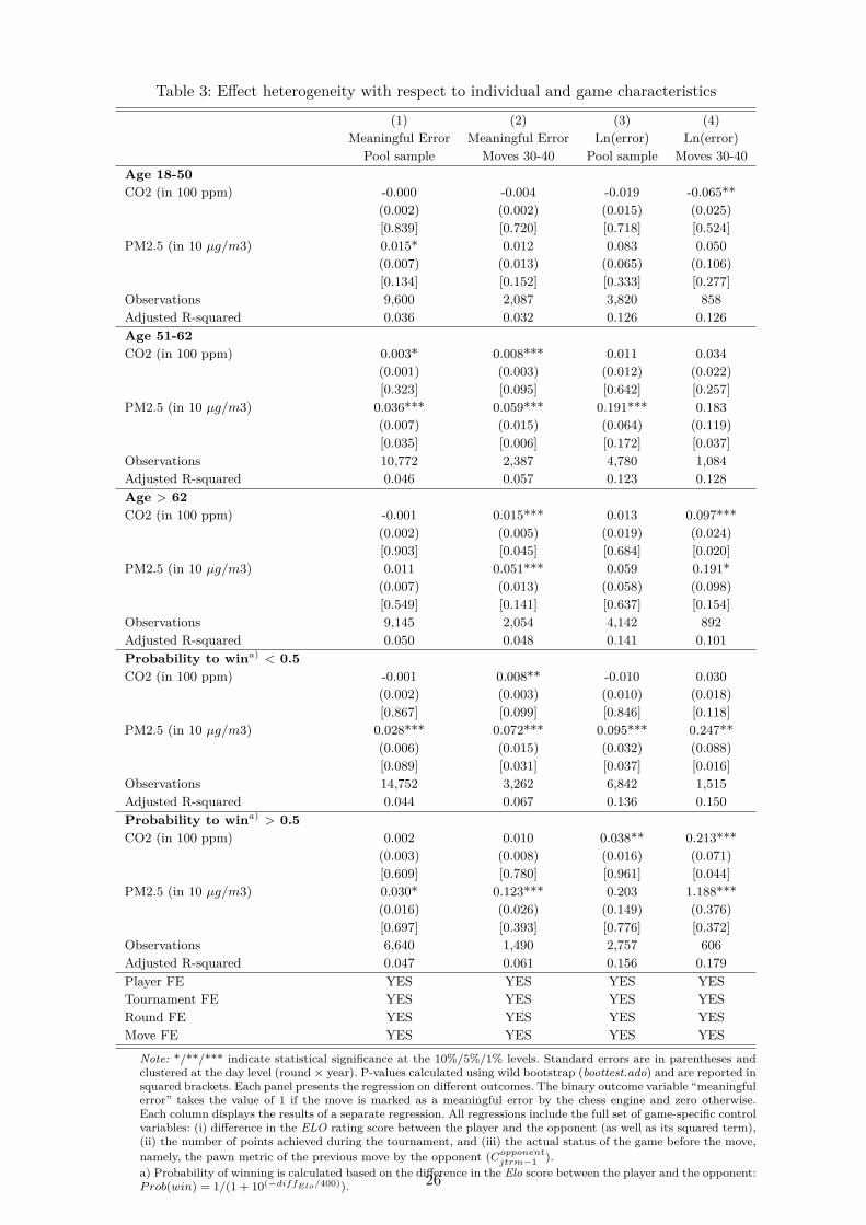
Table 3: Effect heterogeneity with respect to individual and game characteristics

(1) (2) (3) (4)Meaningful Error Meaningful Error Ln(error) Ln(error)

Pool sample Moves 30-40 Pool sample Moves 30-40Age 18-50CO2 (in 100 ppm) -0.000 -0.004 -0.019 -0.065**

(0.002) (0.002) (0.015) (0.025)[0.839] [0.720] [0.718] [0.524]

PM2.5 (in 10 µg/m3) 0.015* 0.012 0.083 0.050(0.007) (0.013) (0.065) (0.106)[0.134] [0.152] [0.333] [0.277]

Observations 9,600 2,087 3,820 858Adjusted R-squared 0.036 0.032 0.126 0.126Age 51-62CO2 (in 100 ppm) 0.003* 0.008*** 0.011 0.034

(0.001) (0.003) (0.012) (0.022)[0.323] [0.095] [0.642] [0.257]

PM2.5 (in 10 µg/m3) 0.036*** 0.059*** 0.191*** 0.183(0.007) (0.015) (0.064) (0.119)[0.035] [0.006] [0.172] [0.037]

Observations 10,772 2,387 4,780 1,084Adjusted R-squared 0.046 0.057 0.123 0.128Age > 62CO2 (in 100 ppm) -0.001 0.015*** 0.013 0.097***

(0.002) (0.005) (0.019) (0.024)[0.903] [0.045] [0.684] [0.020]

PM2.5 (in 10 µg/m3) 0.011 0.051*** 0.059 0.191*(0.007) (0.013) (0.058) (0.098)[0.549] [0.141] [0.637] [0.154]

Observations 9,145 2,054 4,142 892Adjusted R-squared 0.050 0.048 0.141 0.101Probability to wina) < 0.5CO2 (in 100 ppm) -0.001 0.008** -0.010 0.030

(0.002) (0.003) (0.010) (0.018)[0.867] [0.099] [0.846] [0.118]

PM2.5 (in 10 µg/m3) 0.028*** 0.072*** 0.095*** 0.247**(0.006) (0.015) (0.032) (0.088)[0.089] [0.031] [0.037] [0.016]

Observations 14,752 3,262 6,842 1,515Adjusted R-squared 0.044 0.067 0.136 0.150Probability to wina) > 0.5CO2 (in 100 ppm) 0.002 0.010 0.038** 0.213***

(0.003) (0.008) (0.016) (0.071)[0.609] [0.780] [0.961] [0.044]

PM2.5 (in 10 µg/m3) 0.030* 0.123*** 0.203 1.188***(0.016) (0.026) (0.149) (0.376)[0.697] [0.393] [0.776] [0.372]

Observations 6,640 1,490 2,757 606Adjusted R-squared 0.047 0.061 0.156 0.179Player FE YES YES YES YESTournament FE YES YES YES YESRound FE YES YES YES YESMove FE YES YES YES YES

Note: */**/*** indicate statistical significance at the 10%/5%/1% levels. Standard errors are in parentheses andclustered at the day level (round × year). P-values calculated using wild bootstrap (boottest.ado) and are reported insquared brackets. Each panel presents the regression on different outcomes. The binary outcome variable “meaningfulerror” takes the value of 1 if the move is marked as a meaningful error by the chess engine and zero otherwise.Each column displays the results of a separate regression. All regressions include the full set of game-specific controlvariables: (i) difference in the ELO rating score between the player and the opponent (as well as its squared term),(ii) the number of points achieved during the tournament, and (iii) the actual status of the game before the move,namely, the pawn metric of the previous move by the opponent (Copponent

jtrm−1 ).a) Probability of winning is calculated based on the difference in the Elo score between the player and the opponent:P rob(win) = 1/(1 + 10(−diffElo/400)). 26

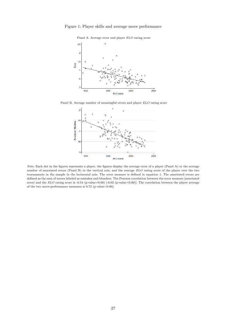
Figure 1: Player skills and average move performance

Panel A. Average error and player ELO rating score

Panel B. Average number of meaningful errors and player ELO rating score

Note: Each dot in the figures represents a player, the figures display the average error of a player (Panel A) or the averagenumber of annotated errors (Panel B) in the vertical axis, and the average ELO rating score of the player over the twotournaments in the sample in the horizontal axis. The error measure is defined in equation 1. The annotated errors aredefined as the sum of moves labeled as mistakes and blunders. The Pearson correlation between the error measure [annotatederror] and the ELO rating score is -0.54 (p-value=0.00) [-0.62 (p-value=0.00)]. The correlation between the player averageof the two move-performance measures is 0.72 (p-value=0.00).

27

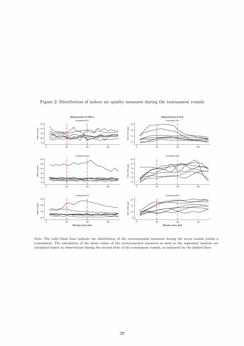
Figure 2: Distribution of indoor air quality measures during the tournament rounds

15

20

25

30

35

PM2.

5 in

µg/

m3

0 60 120 180

Tournament 2017

Measurement of PM2.5

10

15

20

25

CO

2 in

100

x p

pm

0 60 120 180

Tournament 2017

Measurement of CO2

10

20

30

40

50

60

PM2.

5 in

µg/

m3

0 60 120 180

Tournament 2018

10

12

14

16

18

20

CO

2 in

100

x p

pm

0 60 120 180

Tournament 2018

20

40

60

80

PM2.

5 in

µg/

m3

0 60 120 180

Minutes since start

Tournament 2019

5

10

15

20

CO

2 in

100

x p

pm

0 60 120 180

Minutes since start

Tournament 2019

Note: The solid black lines indicate the distribution of the environmental measures during the seven rounds within atournament. The calculation of the mean values of the environmental measures as used in the regression analysis arecalculated based on observations during the second hour of the tournament rounds, as indicated by the dashed lines.

28

Figure 3: Distribution of players’ Elo rating score

0

2

4

6

8

10

Num

ber o

f pla

yers

10001500

12001400

16001800

20002200

23002400

25002700

28823548

1000

2000

2500

Wor

ld C

ham

pion

ship

con

tend

ers

Gra

ndm

aste

rs

Inte

rnat

iona

l Mas

ters

FID

E M

aste

rs

FID

E C

andi

date

Mas

ters

Can

dida

te m

aste

rs

Cla

ss A

Cla

ss B

Cla

ss C

Cla

ss D

novi

ces

Hig

hest

ELO

by

Hum

an

Che

ss e

ngin

e St

ockf

ish

ELO score

Note: The players’ Elo score is calculated by adding 100 to the players’ DWZ score in order to make the scores comparableto the FIDE system.

29

Figure 4: Impact of indoor environmental quality on performance of chess players by move level

Panel A: Meaningful error Panel B: Ln(error)

PM2.5 (in 10 µg/m3)

CO2 concentration (in 100 ppm)

Note: The figure shows the estimated coefficient of joint regressions including PM2.5 and CO2. We divided the total sampleof moves into subsamples with respect to the number of moves within a game (horizontal axis). The vertical, dashed red lineindicates the occurrence of the time restriction during the game. Each panel presents the regression on different outcomes.The binary outcome variable “meaningful error” takes the value of 1 if the move is marked as a meaningful error by thechess engine, and zero otherwise. Dots represent point estimates. Black (gray) bars show the 90% (95%) confidence intervalscalculated based on wild bootstrapping using boottest.ado. All regressions include individual, year, round, and move fixedeffects, as well as the full set of control variables: (i) indoor temperature, humidity and noise, (ii) difference in the ELOrating score between the player and the opponent (as well as its squared term), (iii) the number of points achieved during thetournament, and (iv) the actual status of the game before the move, namely., the pawn metric of the previous move by theopponent (Copponent

jtrm−1 ).

30

Figure 5: Using outdoor pollution measure

Panel A: Meaningful error Panel B: Ln(error)

Outdoor PM10 (in 10 µg/m3)

Note: The figure shows the estimated coefficients of joint regressions including PM10 and CO2. We divided the total sampleof moves into subsamples with respect to the number of moves within a game (horizontal axis). The vertical, dashed red lineindicates the occurrence of the time restriction during the game. Each panel presents the regression on different outcomes.The binary outcome variable “meaningful error” takes on the value one if the move is marked as a meaningful error by thechess engine and zero otherwise. Dots represent point estimates. Black (gray) bars show the 90% (95%) confidence intervalscalculated based on wild bootstrapping using boottest.ado. All regressions include individual, year, round, and move fixedeffects, as well as the full set of control variables: (i) indoor temperature, humidity and noise, (ii) difference in the ELOrating score between the player and the opponent (as well as its squared term), (iii) the number of points achieved during thetournament, and (iv) the actual status of the game before the move, namely., the pawn metric of the previous move by theopponent (Copponent

jtrm−1 ).

31

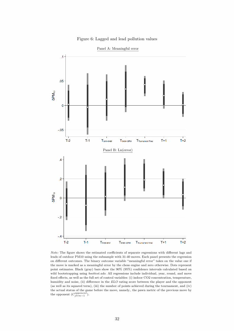
Figure 6: Lagged and lead pollution values

Panel A: Meaningful error

Panel B: Ln(error)

Note: The figure shows the estimated coefficients of separate regressions with different lags andleads of outdoor PM10 using the subsample with 31-40 moves. Each panel presents the regressionon different outcomes. The binary outcome variable “meaningful error” takes on the value one ifthe move is marked as a meaningful error by the chess engine and zero otherwise. Dots representpoint estimates. Black (gray) bars show the 90% (95%) confidence intervals calculated based onwild bootstrapping using boottest.ado. All regressions include individual, year, round, and movefixed effects, as well as the full set of control variables: (i) indoor CO2 concentration, temperature,humidity and noise, (ii) difference in the ELO rating score between the player and the opponent(as well as its squared term), (iii) the number of points achieved during the tournament, and (iv)the actual status of the game before the move, namely., the pawn metric of the previous move bythe opponent (Copponent

jtrm−1 ).

32

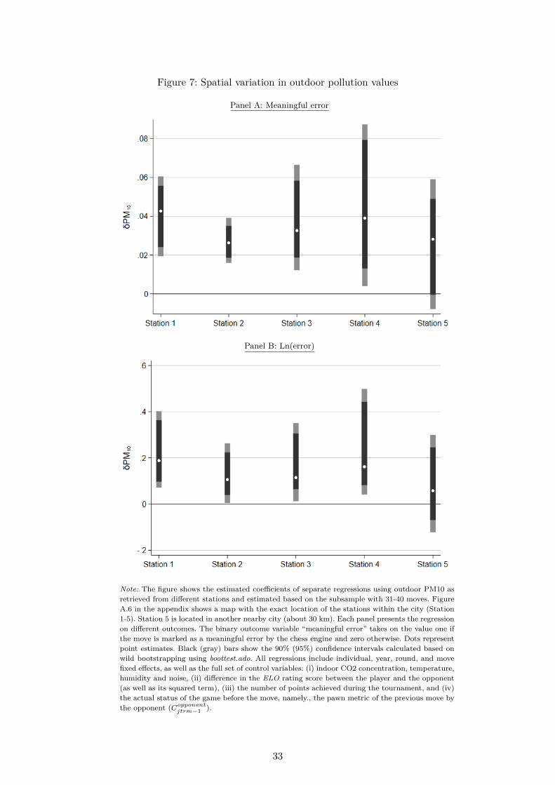
Figure 7: Spatial variation in outdoor pollution values

Panel A: Meaningful error

Panel B: Ln(error)

Note: The figure shows the estimated coefficients of separate regressions using outdoor PM10 asretrieved from different stations and estimated based on the subsample with 31-40 moves. FigureA.6 in the appendix shows a map with the exact location of the stations within the city (Station1-5). Station 5 is located in another nearby city (about 30 km). Each panel presents the regressionon different outcomes. The binary outcome variable “meaningful error” takes on the value one ifthe move is marked as a meaningful error by the chess engine and zero otherwise. Dots representpoint estimates. Black (gray) bars show the 90% (95%) confidence intervals calculated based onwild bootstrapping using boottest.ado. All regressions include individual, year, round, and movefixed effects, as well as the full set of control variables: (i) indoor CO2 concentration, temperature,humidity and noise, (ii) difference in the ELO rating score between the player and the opponent(as well as its squared term), (iii) the number of points achieved during the tournament, and (iv)the actual status of the game before the move, namely., the pawn metric of the previous move bythe opponent (Copponent

jtrm−1 ).

33

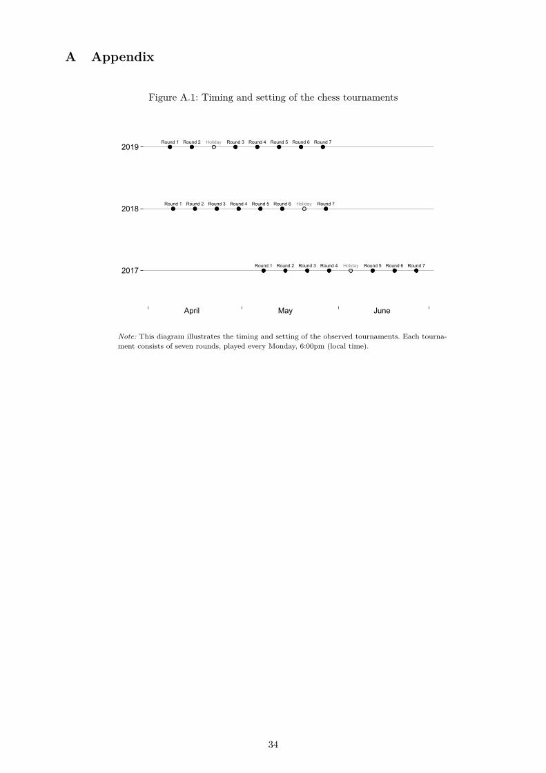
A Appendix

Figure A.1: Timing and setting of the chess tournaments

Round 1 Round 2 Round 3 Round 4 Round 5 Round 6 Round 7

Round 1 Round 2 Round 3 Round 4 Round 5 Round 6 Round 7

Round 1 Round 2 Round 3 Round 4 Round 5 Round 6 Round 7

Holiday

Holiday

Holiday

2017

2018

2019

April May June

Note: This diagram illustrates the timing and setting of the observed tournaments. Each tourna-ment consists of seven rounds, played every Monday, 6:00pm (local time).

34

Figure A.2: Example of players’ hand-written game notation

Note: This picture shows an example of the hand-written documentation as filled in during eachgame within the chess tournament. The documentation has been digitized by the tournamentorganizers.

35

Figure A.3: Distribution of time per move

Note: This diagram shows the distribution of remaining time (in minutes) in clock for a given move.The evidence was collected based on a sample of 63 games played during the 2019 tournamentedition.

Figure A.4: Distribution of total number of moves per game

Note: This diagram shows the distribution of the total number of moves for all thegames in our sample.

36

Figure A.5: Example for sensor location

Note: This picture illustrates the placement of one sensor measuring the indoor environmentalquality. In total, three sensors were placed across the room on separate tables.

Figure A.6: Location of weather and air quality stations within the city of the tournament

Note: This picture shows a map of the city where the observed chess tournaments took place. Thered dot indicates the location of the tournament venue. The blue dots indicate the location of theavailable air quality stations. Station 1 is the main station used to retrieve the outdoor pollutionvalues (about 3.8 km away from the tournament venue).

37

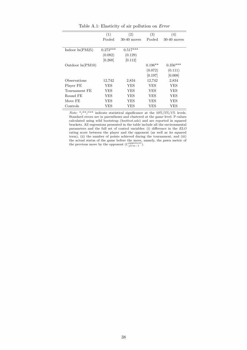
Table A.1: Elasticity of air pollution on Error

(1) (2) (3) (4)Pooled 30-40 moves Pooled 30-40 moves

Indoor ln(PM25) 0.273*** 0.517***(0.082) (0.129)[0.268] [0.112]

Outdoor ln(PM10) 0.196** 0.356***(0.072) (0.111)[0.197] [0.008]

Observations 12,742 2,834 12,742 2,834Player FE YES YES YES YESTournament FE YES YES YES YESRound FE YES YES YES YESMove FE YES YES YES YESControls YES YES YES YES

Note: */**/*** indicate statistical significance at the 10%/5%/1% levels.Standard errors are in parentheses and clustered at the game level. P-valuescalculated using wild bootstrap (boottest.ado) and are reported in squaredbrackets. All regressions presented in the table include all the environmentalparameters and the full set of control variables: (i) difference in the ELOrating score between the player and the opponent (as well as its squaredterm), (ii) the number of points achieved during the tournament, and (iii)the actual status of the game before the move, namely, the pawn metric ofthe previous move by the opponent (Copponent

jtrm−1 ).

38

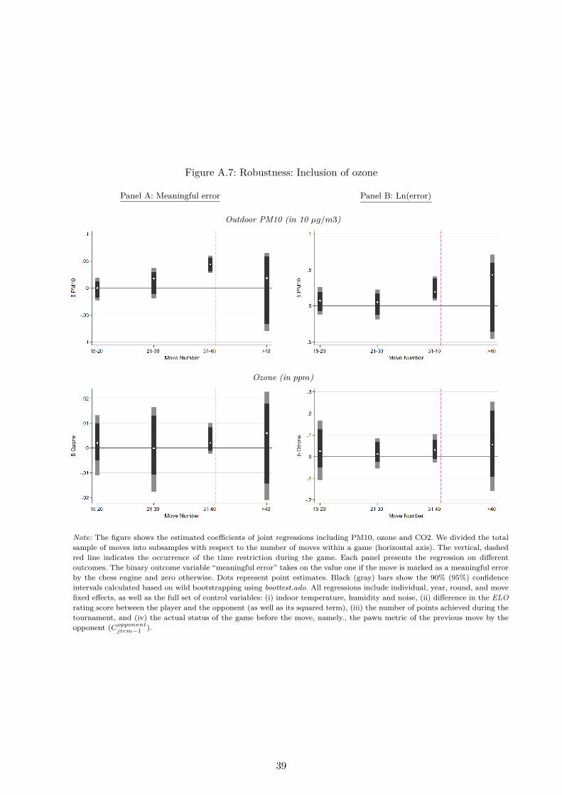
Figure A.7: Robustness: Inclusion of ozone

Panel A: Meaningful error Panel B: Ln(error)

Outdoor PM10 (in 10 µg/m3)

Ozone (in ppm)

Note: The figure shows the estimated coefficients of joint regressions including PM10, ozone and CO2. We divided the totalsample of moves into subsamples with respect to the number of moves within a game (horizontal axis). The vertical, dashedred line indicates the occurrence of the time restriction during the game. Each panel presents the regression on differentoutcomes. The binary outcome variable “meaningful error” takes on the value one if the move is marked as a meaningful errorby the chess engine and zero otherwise. Dots represent point estimates. Black (gray) bars show the 90% (95%) confidenceintervals calculated based on wild bootstrapping using boottest.ado. All regressions include individual, year, round, and movefixed effects, as well as the full set of control variables: (i) indoor temperature, humidity and noise, (ii) difference in the ELOrating score between the player and the opponent (as well as its squared term), (iii) the number of points achieved during thetournament, and (iv) the actual status of the game before the move, namely., the pawn metric of the previous move by theopponent (Copponent

jtrm−1 ).

39

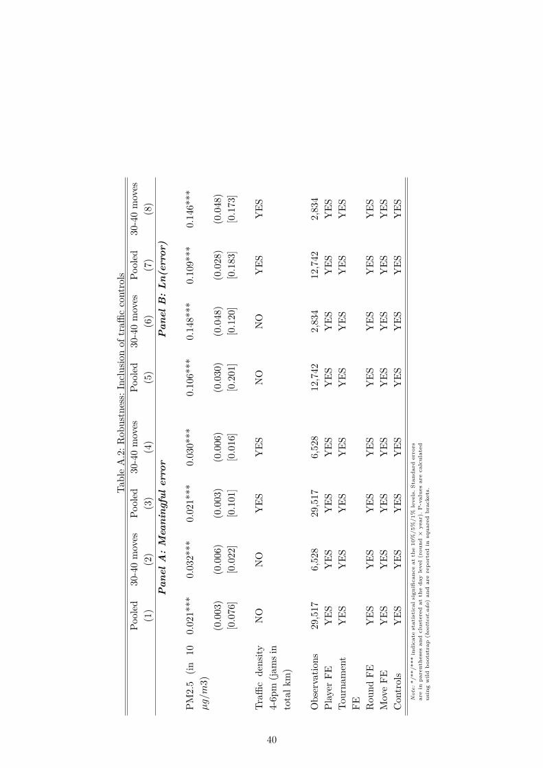
Tabl

eA

.2:R

obus

tnes

s:In

clus

ion

oftr

affic

cont

rols

Pool

ed30

-40

mov

esPo

oled

30-4

0m

oves

Pool

ed30

-40

mov

esPo

oled

30-4

0m

oves

(1)

(2)

(3)

(4)

(5)

(6)

(7)

(8)

Pan

elA

:M

eani

ngfu

ler

ror

Pan

elB

:L

n(er

ror)

PM2.

5(in

10µg/m

3)0.

021*

**0.

032*

**0.

021*

**0.

030*

**0.

106*

**0.

148*

**0.

109*

**0.

146*

**

(0.0

03)

(0.0

06)

(0.0

03)

(0.0

06)

(0.0

30)

(0.0

48)

(0.0

28)

(0.0

48)

[0.0

76]

[0.0

22]

[0.1

01]

[0.0

16]

[0.2

01]

[0.1

20]

[0.1

83]

[0.1

73]

Traffi

cde

nsity

4-6p

m(j

amsi

nto

talk

m)

NO

NO

YES

YES

NO

NO

YES

YES

Obs

erva

tions

29,5

176,

528

29,5

176,

528

12,7

422,

834

12,7

422,

834

Play

erFE

YES

YES

YES

YES

YES

YES

YES

YES

Tour

nam

ent

FEY

ESY

ESY

ESY

ESY

ESY

ESY

ESY

ES

Rou

ndFE

YES

YES

YES

YES

YES

YES

YES

YES

Mov

eFE

YES

YES

YES

YES

YES

YES

YES

YES

Con

trol

sY

ESY

ESY

ESY

ESY

ESY

ESY

ESY

ESN

ote:

*/**

/***

indi

cate

stat

isti

cals

igni

fica

nce

atth

e10

%/5

%/1

%le

vels

.Sta

ndar

der

rors

are

inpa

rent

hese

san

dcl

uste

red

atth

eda

yle

vel

(rou

nd×

year

).P

-val

ues

are

calc

ulat

edus

ing

wild

boo

tstr

ap(b

oott

est.

ado)

and

are

rep

orte

din

squa

red

brac

kets

.

40

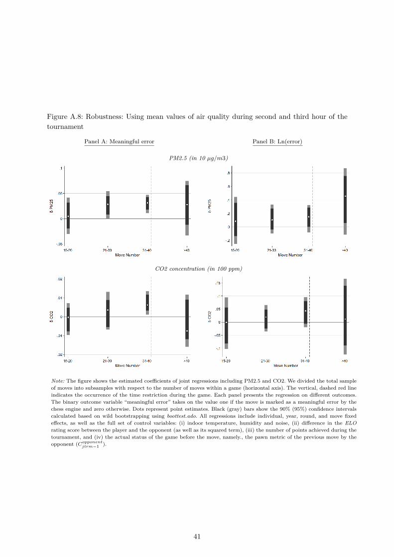
Figure A.8: Robustness: Using mean values of air quality during second and third hour of thetournament

Panel A: Meaningful error Panel B: Ln(error)

PM2.5 (in 10 µg/m3)

CO2 concentration (in 100 ppm)

Note: The figure shows the estimated coefficients of joint regressions including PM2.5 and CO2. We divided the total sampleof moves into subsamples with respect to the number of moves within a game (horizontal axis). The vertical, dashed red lineindicates the occurrence of the time restriction during the game. Each panel presents the regression on different outcomes.The binary outcome variable “meaningful error” takes on the value one if the move is marked as a meaningful error by thechess engine and zero otherwise. Dots represent point estimates. Black (gray) bars show the 90% (95%) confidence intervalscalculated based on wild bootstrapping using boottest.ado. All regressions include individual, year, round, and move fixedeffects, as well as the full set of control variables: (i) indoor temperature, humidity and noise, (ii) difference in the ELOrating score between the player and the opponent (as well as its squared term), (iii) the number of points achieved during thetournament, and (iv) the actual status of the game before the move, namely., the pawn metric of the previous move by theopponent (Copponent

jtrm−1 ).

41

Figure A.9: Robustness: Only games with > 40 moves per player

Panel A: Meaningful error Panel B: Ln(error)

PM2.5 (in 10 µg/m3)

CO2 concentration (in 100 ppm)

Note: The figure shows the estimated coefficients of joint regressions including PM2.5 and CO2. We divided the total sampleof moves into subsamples with respect to the number of moves within a game (horizontal axis). The vertical, dashed red lineindicates the occurrence of the time restriction during the game. Each panel presents the regression on different outcomes.The binary outcome variable “meaningful error” takes on the value one if the move is marked as a meaningful error by thechess engine and zero otherwise. Dots represent point estimates. Black (gray) bars show the 90% (95%) confidence intervalscalculated based on wild bootstrapping using boottest.ado. All regressions include individual, year, round, and move fixedeffects, as well as the full set of control variables: (i) indoor temperature, humidity and noise, (ii) difference in the ELOrating score between the player and the opponent (as well as its squared term), (iii) the number of points achieved during thetournament, and (iv) the actual status of the game before the move, namely., the pawn metric of the previous move by theopponent (Copponent

jtrm−1 ).

42