Distance Correlation: A New Tool for Detecting Associationand Measuring Correlation Between Data Sets

Donald Richards

Penn State University

– p. 1/44

This talk is about “cause” and “effect”

Does “smoking” cause “lung cancer”?

Do “strong gun laws” lower “homicide rates”?

Does “aging” raise “male unemployment rates”?

The difficulty of establishing causation has fascinated mankindsince time immemorial.

Democritus: “I would rather discover one cause than gain thekingdom of Persia.”

– p. 2/44

A simpler problem: Establishing association.

The variables X and Y are associated if changes in one of themtend to be accompanied by changes in the other.

Positive association: Higher values of X tend to beaccompanied by higher values of Y .

Negative association: Higher values of X tend to beaccompanied by lower values of Y .

– p. 3/44

Causation implies association.

But association does not imply causation.

“Foot size” and “Reading ability” are positively associated, butbig feet do not cause higher reading ability.

Nor does better reading ability cause feet to grow larger.

– p. 4/44

There are numerous ways to detect whether two variables areassociated.

Scatterplots

Graphs

Correlations coefficients

Hypothesis testing

An example of hypothesis testing: Is this deck of cards “fair”?

– p. 5/44

Are “Smoking rate” and “lung cancer rate” associated?

Here is a scary graph:

– p. 6/44

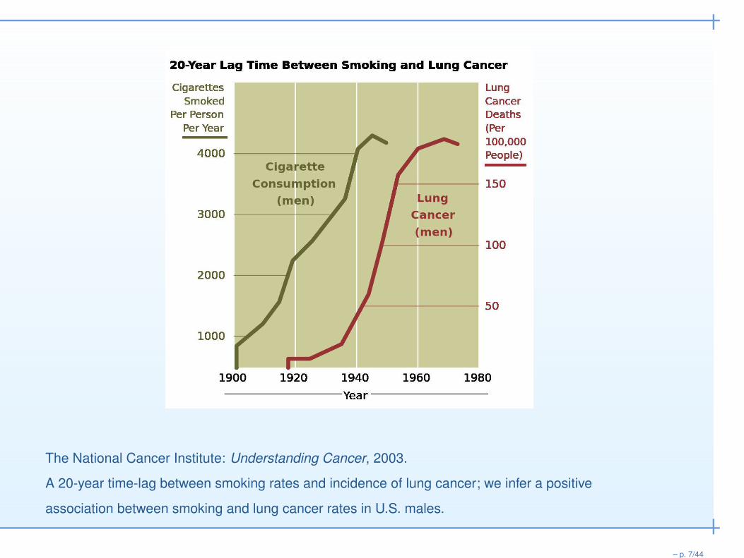
The National Cancer Institute: Understanding Cancer, 2003.

A 20-year time-lag between smoking rates and incidence of lung cancer; we infer a positive

association between smoking and lung cancer rates in U.S. males.

– p. 7/44

How about “Strength of gun laws” and “Homicide rate”?

Here is another thought-provoking graph:

– p. 8/44

Eugene Volokh, “Zero correlation between state homicide rate and state gun laws,” The Washington

Post, Oct. 6, 2015.

– p. 9/44

Lawrence H. Summers, “A disaster is looming for American men,” The Washington Post, Sept. 26,

2016.

– p. 10/44

These two examples are invalid applications of linear regression.

They violate the mathematical assumptions underlying linearregression.

No analysis of potential outlier points or heterogeneity of they-values.

Invalid use of the Pearson correlation coefficient.

It is often unwise to apply linear regression to percentage data.

– p. 11/44

Random variables: X and Y

X: The average height of a randomly chosen couple

Y : The height of that couple’s adult child

µ1 = E(X): The population mean of X

µ2 = E(Y ): The population mean of Y

Var(X) = E[(X − µ1)2]: The population variance of X

Cov(X,Y ) = E[(X −µ1)(Y −µ2)]: Covariance between X and Y

– p. 12/44

The Pearson correlation coefficient:

ρ =Cov(X,Y )

√

Var(X) ·√

Var(Y )

A random sample from (X,Y ): (x1, y1), . . . , (xn, yn)

Sample means: x =1

n

n∑

i=1

xi, y =1

n

n∑

i=1

yi

The empirical Pearson correlation coefficient:

r =1n

∑ni=1(xi − x)(yi − y)

√

1n

∑ni=1(xi − x)2 ·

√

1n

∑ni=1(yi − y)2

– p. 13/44

The Pearson coefficient is unchanged if we shift or dilate the x-or y-values.

The coefficient is very useful for graphical data analysis.

These graphical methods led Galton to discover regression tothe mean.

However, the coefficient applies to scalar random variables, only.

The coefficent often is inapplicable if (X,Y ) are non-linearlyrelated, e.g., “College faculty salaries” and “Liquor sales.”

Even if r = 0, we cannot infer independence between X and Y .

– p. 14/44

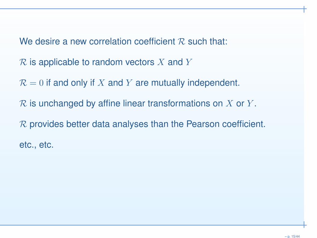
We desire a new correlation coefficient R such that:

R is applicable to random vectors X and Y

R = 0 if and only if X and Y are mutually independent.

R is unchanged by affine linear transformations on X or Y .

R provides better data analyses than the Pearson coefficient.

etc., etc.

– p. 15/44

Distance correlation

Feuerverger (1993), Székely, Rizzo, and Bakirov (2007, 2009)

p and q: positive integers

Column vectors: s = (s1, . . . , sp)′ ∈ R

p, t = (t1, . . . , tq)′ ∈ R

q

Euclidean norms:

‖s‖ = (s21 + · · ·+ s2p)1/2 and ‖t‖ = (t21 + · · ·+ t2q)

1/2

– p. 16/44

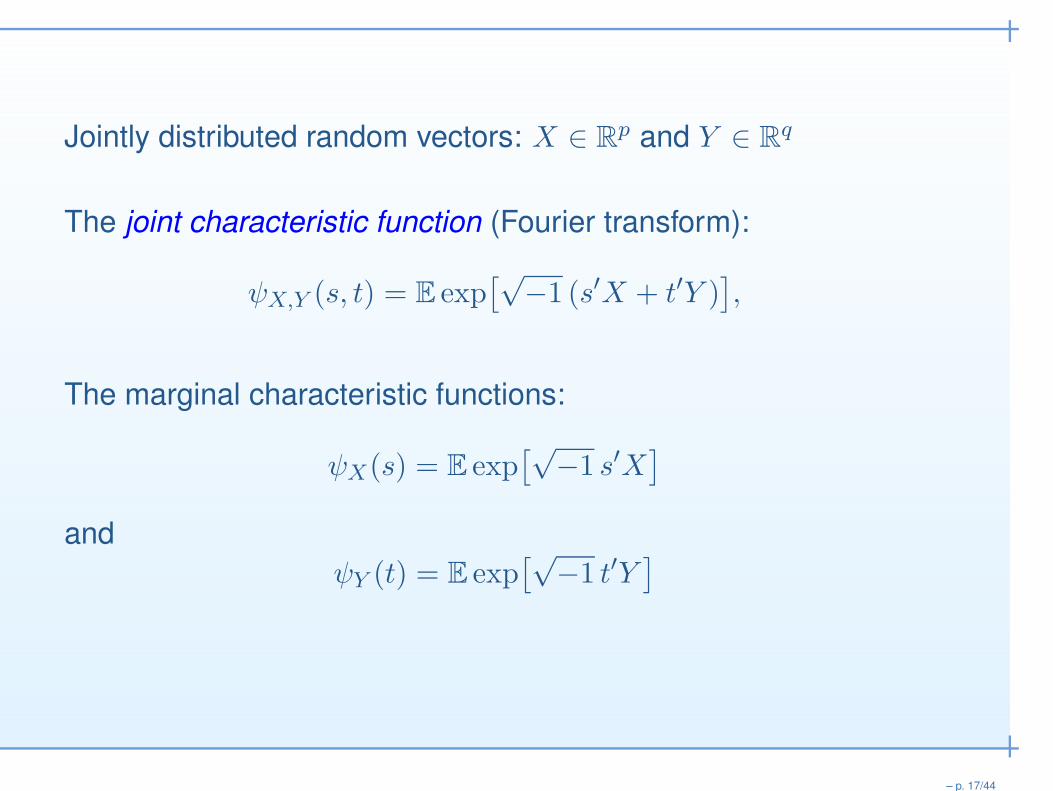
Jointly distributed random vectors: X ∈ Rp and Y ∈ R

q

The joint characteristic function (Fourier transform):

ψX,Y (s, t) = E exp[√

−1 (s′X + t′Y )]

,

The marginal characteristic functions:

ψX(s) = E exp[√

−1 s′X]

andψY (t) = E exp

[√−1 t′Y

]

– p. 17/44

A well-known result: X and Y are mutually independent iff

ψX,Y (s, t) = ψX(s)ψY (t)

for all s and t.

We will measure (X,Y ) dependence by a weighted L2-distance:∥

∥ψX,Y (s, t)− ψX(s)ψY (t)∥

∥

L2(Rp×Rq)

– p. 18/44

The distance covariance between X and Y :

V(X,Y ) =

[

1

γpγq

∫

Rp+q

∣

∣ψX,Y (s, t)− ψX(s)ψY (t)∣

∣

2 ds

‖s‖p+1

dt

‖t‖q+1

]1/2

where γp is a suitable constant.

This definition makes sense even if X = Y .

The distance variance of X:

V(X,X) =

[

1

γ2p

∫

R2p

∣

∣ψX(s+ u)− ψX(s)ψX(u)∣

∣

2 ds

‖s‖p+1

du

‖u‖p+1

]1/2

– p. 19/44

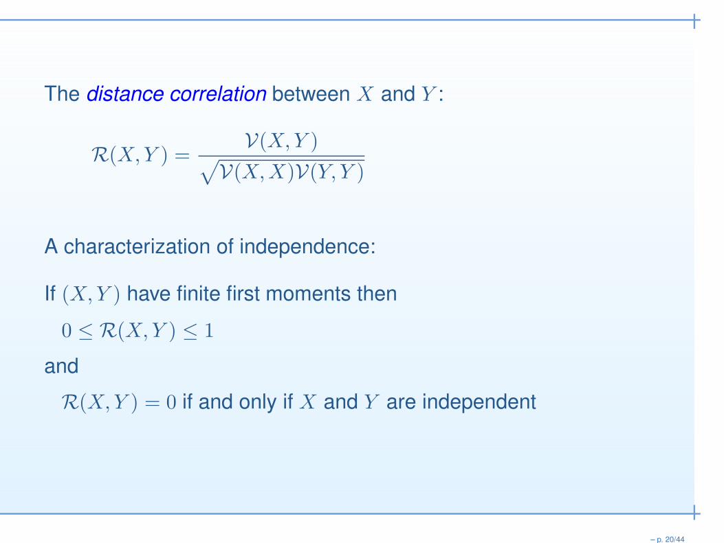
The distance correlation between X and Y :

R(X,Y ) =V(X,Y )

√

V(X,X)V(Y, Y )

A characterization of independence:

If (X,Y ) have finite first moments then

0 ≤ R(X,Y ) ≤ 1

and

R(X,Y ) = 0 if and only if X and Y are independent

– p. 20/44

An Invariance Property:

R(X,Y ) is invariant under the transformation

(X,Y ) 7→ (a1 + b1C1X, a2 + b2C2Y )

where a1 ∈ Rp, a2 ∈ R

q; non-zero b1, b2 ∈ R; and C1 ∈ Rp×p

and C2 ∈ Rq×q are orthogonal matrices.

Note: R(X,Y ) is not invariant under all affine transformations.

– p. 21/44

Calculating Pearson’s correlation coefficient often is easy.

Calculating the distance correlation coefficient often is difficult.

The singular integral∫

Rp+q

∣

∣ψX,Y (s, t)− ψX(s)ψY (t)∣

∣

2 ds

‖s‖p+1

dt

‖t‖q+1

cannot be calculated by expanding the factor

∣

∣ψX,Y (s, t)− ψX(s)ψY (t)∣

∣

2

and then integrating term-by-term.

Dueck, Edelmann, and D.R., J. Multivariate Analysis, 2017

– p. 22/44

The empirical distance correlation

Random sample: (X1, Y 1), . . . , (Xn, Y n) from (X,Y )

Data matrices: X = [X1, . . . ,Xn], Y = [Y 1, . . . , Y n]

The empirical joint characteristic function:

ψX,Y (s, t) =1

n

n∑

j=1

exp[√

−1 (s′Xj + t′Y j)]

The empirical marginal characteristic functions:

ψX(s) =1

n

n∑

j=1

exp[√

−1 s′Xj

]

, ψY (t) =1

n

n∑

j=1

exp[√

−1 t′Y j

]

– p. 23/44

The empirical distance covariance:

Vn(X,Y ) =

[

1

γpγq

∫

Rp+q

|ψX,Y (s, t)− ψX(s)ψY (t)|2 ds

‖s‖p+1

dt

‖t‖q+1

]1/2

ψX,Y , ψX , and ψY are sums of exponential terms.

Vn(X,Y ) surely has to be a complicated function of the data.

And yet, . . .

Feuerverger (1993), Székely, et al. (2007) derived an explicitformula for Vn(X,Y ):

– p. 24/44

Define

akl = ‖Xk −X l‖, ak· =1

n

n∑

l=1

akl, a·l =

1

n

n∑

k=1

akl

a··=

1

n2

n∑

k,l=1

akl, Akl = akl − ak· − a·l + a

··

Define bkl = ‖Y k − Y l‖, bk·, b·l, b··, and Bkl similarly. Then,

Vn(X,Y ) =1

n

( n∑

k,l=1

AklBkl

)1/2

[

Vn(X,Y )]2 is the average entry in the Schur product of thecentered distance matrices for X and Y .

– p. 25/44

A crucial singular integral: For x ∈ Rp and Re(α) ∈ (0, 2),

∫

Rp

‖s‖−(p+α)[

1− exp(√−1s′x)

]

ds = const. ‖x‖α,

with absolute convergence for all x.

Ongoing work with Dueck, Edelmann, Sahi: Generalizations tomatrix spaces and symmetric cones.

– p. 26/44

The empirical distance correlation:

Rn(X,Y ) =Vn(X,Y )

√

Vn(X,X)Vn(Y ,Y )

Some properties:

• 0 ≤ Rn(X,Y ) ≤ 1

• Rn(X,Y ) = 1 implies that:

(a) p = q,

(b) The linear spaces spanned by X and Y have full rank, and

(c) There exists an affine relationship between X and Y .

– p. 27/44

The distance correlation coefficient has been found to:

Exhibit higher statistical power (i.e., fewer false positives) thanthe Pearson coefficient

Detect nonlinear associations that were not found by thePearson coefficient, and

Locate smaller sets of variables that provide equivalentstatistical information.

– p. 28/44

Astrophysical data

Mercedes Richards, Elizabeth Martínez-Gómez, and D.R., Astrophysical Journal, 2014

The COMBO-17 database

“Classifying Objects by Medium-Band Observations in 17 filters”

High-dimensional data on many astrophysical objects in theChandra Deep Field South.

– p. 29/44

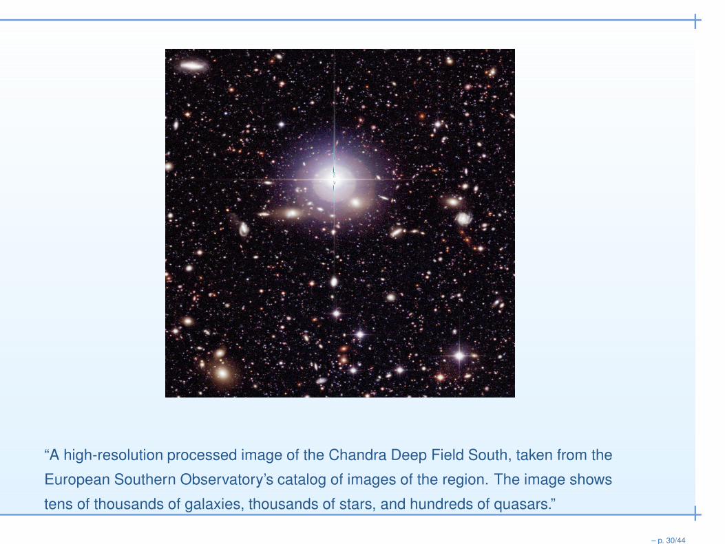
“A high-resolution processed image of the Chandra Deep Field South, taken from the

European Southern Observatory’s catalog of images of the region. The image shows

tens of thousands of galaxies, thousands of stars, and hundreds of quasars.”

– p. 30/44

The COMBO-17 database

Astrophysical observations on 63,501 galaxies, stars,quasars, and other unclassified objects, with variousbrightness measurements in 17 “passbands” over thewavelength range 3500 - 9300Å (Wolf, et al. 2003)

Why do astronomers collect brightness measurementsat many different wavelengths?

– p. 31/44

The Crab Nebula, from the supernova of 1054 AD

– p. 32/44

General Information

Rmag Total R-band magnitudemu_max Central surface brightnessMajAxis Major axisMinAxis Minor axisPA Position angle

Classification Results

MC_z Mean redshift in distribution p(z)MC_z2 Alternative redshift if distribution p(z) is bimodalMC_z_ml Peak redshift in distributiondl Luminosity distance of MC_z

Total Object Restframe Luminosities

BjMag Mabs,gal in Johnson B (z ≈ [0.0,1.1])

rsMag Mabs,gal in SDSS r (z ≈ [0.0,0.5])

S280Mag Mabs,gal in 280/40 (z ≈ [0.25,1.3])

Observed Seeing-Adaptive Aperture Fluxes

W420F_E Photon flux in filter 420 in run EW462F_E Photon flux in filter 462 in run EW485F_D Photon flux in filter 485 in run DW518F_E Photon flux in filter 518 in run EW571F_D Photon flux in filter 571 in run DW571F_E Photon flux in filter 571 in run EW604F_E Photon flux in filter 604 in run EW646F_D Photon flux in filter 646 in run DW696F_E Photon flux in filter 696 in run EW753F_E Photon flux in filter 753 in run EW815F_E Photon flux in filter 815 in run EW856F_D Photon flux in filter 856 in run DW914F_D Photon flux in filter 914 in run DW914F_E Photon flux in filter 914 in run EUF_F Photon flux in filter U in run FBF_D Photon flux in filter B in run DBF_F Photon flux in filter B in run FVF_D Photon flux in filter V in run DRF_D Photon flux in filter R in run DRF_E Photon flux in filter R in run ERF_F Photon flux in filter R in run F

– p. 33/44

Type 1: Elliptical, bulge S0Type 2: Spiral: Sa–SbcType 3: Spiral: SbcType 4: Starburst

Number of galaxies by type and redshift

Type of Galaxies

Redshift Type 1 Type 2 Type 3 Type 4 Total

0 ≤ z < 0.5 38 45 328 3254 36650.5 ≤ z < 1 50 19 277 9284 96301 ≤ z < 2 16 4 109 1928 2057

Total 104 68 714 14466 15352

– p. 34/44

33 variables

Number of pairs of variables:(

33

2

)

= 528

For each of these 528 pairs, and for each of the 12 combinationsof (Redshift, Galaxy Type), we calculated the empirical:

Pearson correlation coefficient

MIC (maximal information coefficient)

Distance correlation coefficient

– p. 35/44

Exploratory distance correlation analysis for some COMBO-17 data

Plots of Pearson correlation coefficients vs. MIC scores (top row) and vs. distance

correlation (bottom row) for redshifts z ∈ [0, 0.5) and three types of galaxies.

– p. 36/44

The distance correlation coefficient was superior to othermeasures of correlation in resolving data into concentratedhorseshoe- or V-shapes.

This led to more accurate classification of galaxies andidentification of outlying pairs of variables.

These results held for a range of redshifts beyond the LocalUniverse and for galaxies ranging from elliptical to spiral.

The Types 2 and 3 spiral galaxies seem to be contaminated byType 4 starburst galaxies, consistent with earlier findings ofother astrophysicists.

We found further evidence of this contamination from theV-shaped scatter plots for galaxies of Types 2 or 3.

– p. 37/44

The subplots for each galaxy type are shown in the four middleframes, and their superposition in the large left frame.

Potential outlying pairs in the scatter plot for Type 3 galaxies arecircled in the large right frame.

– p. 38/44

Return to “Strength of state gun laws” and “State homicide rate”

Wouldn’t it be better to analyze the relationship between “Strength of state gun laws” and

“All gun-related deaths”?

– p. 39/44

Horizontal: All gun-related deaths (per 100,000 people), by state and D.C.

Vertical: Brady Campaign gun law score for each state and D.C.

– p. 40/44

We applied several measures of correlation to the data on“Strength of state gun laws” vs. “State homicide rate”

None of these measures were able to detect a statisticallysignificant relationship between these two variables.

We applied these measures of correlation to the data on“Strength of state gun laws” vs. “All gun-related deaths”.

All of these measures reported a statistically significantrelationship.

All the corresponding p-values were nearly zero.

– p. 41/44

Distance correlation has its limitations.

Logistic regression: Estimating odds ratios.

If the patient exhibits certain symptoms then the odds are highthat immediate surgery is called for.

If interest rates are below 4% and . . . then the odds are high thatyou are better off buying rather than renting.

If . . . then . . .

Dominic Edelmann: Simulations which suggest that logisticregression often is better than distance correlation at findingthe variables that are better suited for estimating odds ratios.

– p. 42/44

To complicate matters, statistical methods can flip-flopdepending on the time horizon.

If interest rates are above 12% and . . . then the odds are highthat you are better off renting, but only over the short-term.

Distance correlation, or other statistical methods, cannot easilyresolve short-term vs. long-term decisions.

My advice: Also listen to those who have extensive practicalexperience in these matters.

– p. 43/44

References

Dueck, J., Edelmann, D., and Richards, D. (2017). Distance correlation coefficients for Lancasterdistributions. Journal of Multivariate Analysis, vol. 154, 19–39.

Feuerverger, A. (1993). A consistent test for bivariate dependence. International Statistical Review ,vol. 61, 419–433.

Martínez-Gómez, E., Richards, M. T., and Richards, D. (2014). Distance correlation methods fordiscovering associations in large astrophysical databases. Astrophysical Journal , vol. 781, 39

Richards, M. T., Richards, D., and Martínez-Gómez, E. (2014). Interpreting the distance correlationresults for the COMBO-17 survey. Astrophysical Journal Letters, vol. 784

Rizzo, M. L. and Székely, G. J. (2011). E-statistics. R package, Version 1.4-0;http://cran.us.r-project.org/web/packages/energy/index.html.

Székely, G. J., Rizzo, M. L. and Bakirov, N. K. (2007). Measuring and testing independence bycorrelation of distances. Annals of Statistics, vol. 35, 2769–2794.

Székely, G. J. and Rizzo, M. (2009). Brownian distance covariance. Annals of Applied Statistics, vol.3, 1236–1265.

Wolf, C., et al. (2003). The COMBO-17 database. Astronomy & Astrophysics, vol. 401, 73–98.

– p. 44/44