distortion-induced fatigue investigation of double …
TRANSCRIPT

The Pennsylvania State University
The Graduate School
College of Engineering
DISTORTION-INDUCED FATIGUE INVESTIGATION OF DOUBLE ANGLE
STRINGER-TO-FLOORBEAM CONNECTIONS
A Thesis in
Civil Engineering
by
Robert C. Guyer
© 2010 Robert C. Guyer
Submitted in Partial Fulfillment of the Requirements
for the Degree of
Master of Science
December 2010

The thesis of Robert C. Guyer was reviewed and approved* by the following: Jeffrey A. Laman Professor of Civil Engineering Thesis Advisor Thomas E. Boothby Professor of Architectural Engineering Andrew Scanlon Professor of Civil Engineering Peggy Johnson Professor of Civil Engineering Head of the Department of Civil and Environmental Engineering *Signatures on file in the Graduate School

iii
ABSTRACT
Past research has shown that double angle stringer-to-floorbeam connections in riveted
railway bridges are susceptible to fatigue cracking caused by secondary, distortion induced
stress. This stress, caused by stringer end rotation is not easily calculable therefore more detailed
analysis techniques are needed to quantify connection behavior. The present study was initiated
to determine the effect of connection parameters on moment-rotation behavior and stress
concentrations from a standard 286,000 pound railcar load. Seventy-two unique double angle
connection configurations were investigated using ABAQUS 3D and SAP2000 2D finite element
analysis software. Two double angle connection specimens were evaluated experimentally that
provided verification data for finite element model calibration. Parametric study results are
presented as moment-rotation curves and compared with three empirical prediction equations.
Maximum principal stress is investigated in each analysis case and a stress prediction equation is
proposed. This equation provides an easily calculable and effective method to predict the
magnitude of stress range in connection angles as a function of study parameters: (1) outstanding
gage distance, (2) angle depth, (3) angle thickness, and (4) stringer length. This facilitates
fatigue life evaluation without the need for rigorous analysis. Additionally, study parameters are
quantified and compared to the current AREMA fatigue design rule.

iv
TABLE OF CONTENTS
LIST OF FIGURES .................................................................................................... viii LIST OF TABLES ......................................................................................................... xi ACKNOWLEDGEMENTS ......................................................................................... xii Chapter 1. INTRODUCTION ......................................................................................... 1
1.1 General Background ........................................................................................... 1 1.2 Problem Statement .............................................................................................. 6
1.3 Scope of Research ............................................................................................... 7 1.4 Objectives ........................................................................................................... 9 Chapter 2. LITERATURE REVIEW ............................................................................ 11 2.1 Introduction ...................................................................................................... 11 2.2 Brief History of Bridge Loading ...................................................................... 12 2.3 Fatigue Prone Detail: Double Angle Connection ............................................. 14 2.4 Fatigue............................................................................................................... 15 2.4.1 Introduction .............................................................................................. 15 2.4.2 Fatigue Studies ......................................................................................... 17 2.5 Design of Connection Angles ........................................................................... 25 2.6 Bridge Field and Case Studies of Double Angle Connection ........................... 26 2.6.1 Highway Bridges ..................................................................................... 26 2.6.2 Railway Bridges ....................................................................................... 28 2.7 Moment – Rotation Behavior of Double Angle Connections ........................... 32 2.7.1 Connection Stiffness, K ........................................................................... 32 2.7.2 Connection Strength................................................................................. 34 2.7.3 Connection Ductility ................................................................................ 34 2.7.4 Derivation of Moment – Rotation Curves ............................................... 34 2.8 Finite Element Modeling of Double Angle Connections ................................. 39 2.8.1 Introduction .............................................................................................. 39 2.8.2 Finite Element Modeling ......................................................................... 39 2.9 Experimental Laboratory Evaluation of Double Angle Connections ............... 43 2.10 Summary ......................................................................................................... 44 Chapter 3. STUDY DESIGN ........................................................................................ 47 3.1 Introduction ....................................................................................................... 47 3.2 Determination of Parameters ............................................................................ 47 3.2.1 Primary Independent Parameters ............................................................. 47 3.2.1.1 Stringer Length, L ........................................................................... 48 3.2.1.2 Angle Thickness, t .......................................................................... 48 3.2.1.3 Gage Distance of the Outstanding Leg, g ....................................... 48

v
3.2.1.4 Angle Depth, d ................................................................................ 50 3.2.1.5 Parametric Study Independent Parameter Combinations ............... 52 3.2.2 Dependent Parameters ............................................................................. 53 3.2.2.1 Rivet Spacing, Number of Rivets, Angle Leg Length .................... 54 3.2.2.2 Stringer Stiffness ............................................................................. 56 3.2.3 Non-Variable Parameters ......................................................................... 58 3.2.3.1 Rivet Diameter ................................................................................ 59 3.2.3.2 Rivet Clamping Force ..................................................................... 59 3.2.3.3 Friction Coefficient ......................................................................... 59 3.2.3.4 Material Constants .......................................................................... 60 3.2.1.5 Fatigue Vehicle ............................................................................... 60 3.3 Parametric Study Framework ........................................................................... 60 3.3.1 Procedure ................................................................................................. 61 3.4 Summary ........................................................................................................... 66 Chapter 4. EXPERIMENTAL DESIGN AND TESTING ........................................... 67 4.1 Introduction ....................................................................................................... 67 4.2 Experimental Test Design and Specimens ........................................................ 67 4.3 Test Set-Up and Instrumentation ...................................................................... 70 4.4 Test Procedure .................................................................................................. 74 4.5 Experimental Test Results ................................................................................ 75 4.5.1 Specimen 1 Results .................................................................................. 75 4.5.2 Specimen 2 Results .................................................................................. 78 4.6 Summary ........................................................................................................... 80 Chapter 5. NUMERICAL MODELING ....................................................................... 81 5.1 Introduction ....................................................................................................... 81 5.2 3D FE Model Validation ................................................................................... 82 5.2.1 FE Model Description .............................................................................. 82 5.2.1.1 FE Model Part: Connection Angle .................................................. 83 5.2.1.2 FE Model Part: Fastener ................................................................. 84 5.2.1.3 FE Model Part: Stringer Web ........................................................ 85 5.2.1.4 FE Model Part: Mounting Flange ................................................... 86 5.2.1.5 Boundary Conditions ...................................................................... 86 5.2.1.6 Contact Interaction .......................................................................... 87 5.2.1.7 Applied Load .................................................................................. 87 5.2.2 Comparison with Experimental Results................................................... 88 5.2.3 Discussion ................................................................................................ 91 5.3 Parametric Study 3D FE Modeling ................................................................... 95 5.4 Parametric Study 2D FE Modeling ................................................................... 95 5.5 Results ............................................................................................................... 96 5.5.1 Parametric Study Moment-Rotation Results ........................................... 96 5.5.2 Parametric Study Principal Stress Results ............................................. 100 5.6 Summary ......................................................................................................... 102

vi
Chapter 6. ANALYSIS AND DISCUSSION OF RESULTS .................................... 103 6.1 Introduction ..................................................................................................... 103 6.2 Moment-Rotation Prediction .......................................................................... 103 6.3 Connection Classification ............................................................................... 104 6.4 Parameter Influence on Connection Behavior ................................................ 105 6.5 Investigation of Current Design Equation ...................................................... 109 6.6 Stress Prediction Equation .............................................................................. 111 6.7 Summary ......................................................................................................... 114 Chapter 7. SUMMARY AND CONCLUSIONS........................................................ 116 7.1 Summary ......................................................................................................... 116 7.2 Conclusions .................................................................................................... 118 7.3 Recommendations for Future Research .......................................................... 120 Appendix: RESULTS – TABLES AND GRAPHS ................................................... 122 Bibliography .............................................................................................................. 134
vii
LIST OF FIGURES Figure 1.1 Typical Girder-Floorbeam-Stringer Bridge Framing .................................... 2 Figure 1.2 Typical Girder-Floorbeam-Stringer Railway Bridge (Underside View) ....... 3 Figure 1.3 Typical Stringer-to-Floorbeam Double Angle Connection Schematic ......... 5 Figure 1.4 Typical Stringer-to-Floorbeam Double Angle Connection ........................... 5 Figure 1.5 Typical Distortion-Induced Fatigue Crack in Double Angle Connection
[AREMA, 2008b reprinted with permission] ..................................................... 6 Figure 2.1 AREMA Cooper E-80 Design Live Load [AREMA, 2008a reprinted
with permission ................................................................................................. 12 Figure 2.2 Typical Rail Car Loads (provided by Norfolk Southern Railroad, Inc.) ..... 13 Figure 2.3 SR-N Curves for Fatigue Categories [AREMA, 2008a reprinted with
permission] ........................................................................................................ 16 Figure 2.4 Typical Riveted, Built-up “I” Section ......................................................... 18 Figure 2.5 Diagram of Fatigue Specimens [Wilson, 1940] .......................................... 21 Figure 2.6 Assumed Action of Angles Used in Computing Flexural Stress and Deflection [Wilson, 1940] ................................................................................ 23 Figure 2.7 Definitions of Stiffness, Strength, and Ductility Characteristics of the Moment-Rotation Response of a Connection (Copyright © American Institute of Steel Construction Reprinted with permission. All rights reserved.) ........................................................................................................... 33 Figure 2.8 Classification of Moment-Rotation Response of Fully Restrained (FR), Partially Restrained (PR), and Simple Connections (Copyright © American Institute of Steel Construction Reprinted with permission. All rights reserved.) ........................................................................................................... 33 Figure 2.9 Moment-Rotation Schematic for Cantilevered Beam with Double Angle Connection ............................................................................................ 35 Figure 3.1 Schematic of Typical Double Angle Connection in Plan ............................ 49 Figure 3.2 Descriptions of Test Angles ........................................................................ 56
viii
Figure 3.3 Laboratory Testing of Double Angle Connection ....................................... 61 Figure 3.4 Typical 3D FE Connection Model Assembly (ABAQUS) ......................... 62 Figure 3.5 Typical Moment-Rotation Curve ................................................................ 63 Figure 3.6 Service Load Connection Secant Stiffness, Ks ............................................ 64 Figure 3.7 Typical 2D FE Stringer Beam Model (SAP2000) ....................................... 65 Figure 4.1 Experimental Test Design ........................................................................... 68 Figure 4.2 Experimental Test Specimen 1 .................................................................... 69 Figure 4.3 Detail of Strain Gage Placement on Test Specimen 1 ................................. 70 Figure 4.4 Installed Strain Gages, Specimen 1 ............................................................. 70 Figure 4.5 Detail of Strain Gage Placement on Test Specimen 2 ................................. 71 Figure 4.6 Installed Strain Gages, Specimen 2 ............................................................. 72 Figure 4.7 Angle Rotation Measurement -- Detail of Dial Gage Placement ................ 73 Figure 4.8 Angle Rotation Measurement -- Dial Gage Placement Photo ..................... 74 Figure 4.9 Lab Specimen 1: Moment-Rotation Curve .................................................. 75 Figure 4.10 Lab Specimen 1: Filtered Strain (stress) vs Moment ................................ 76 Figure 4.11 Specimen Mounting Surface ..................................................................... 77 Figure 4.12 Bolt Hole Misalignment in Specimen 1 .................................................... 78 Figure 4.13 Lab Specimen 2: Moment-Rotation Curve................................................ 78 Figure 4.14 Lab Specimen 2: Averaged, Filtered Strain (stress) vs Moment ............... 79 Figure 5.1 Typical 3D FE Connection Model Assembly ............................................. 82 Figure 5.2 Meshed Connection Angle (ABAQUS) ...................................................... 83 Figure 5.3 Meshed Fastener (ABAQUS) ...................................................................... 84 Figure 5.4 Rigid Body Stringer Web (ABAQUS) ........................................................ 85

ix
Figure 5.5 Rigid Body Mounting Flange (ABAQUS) .................................................. 86 Figure 5.6 Specimen 1: Moment-Rotation of Experimental and Numerical ................ 89 Figure 5.7 Specimen 1: Experimental vs Numerical - All Gage Locations .................. 89 Figure 5.8 Specimen 2: Moment-Rotation of Experimental and Numerical ................ 90 Figure 5.9 Specimen 2: Experimental vs Numerical – All Gage Locations ................. 90 Figure 5.10 Specimen 2: Deformed Shape Comparison – Experimental and Numerical .......................................................................................................... 91 Figure 5.11 2D FE Stringer Beam Model ..................................................................... 96 Figure 5.12 Numerical Moment-Rotation Curves for d=10" ........................................ 97 Figure 5.13 Numerical Moment-Rotation Curves for d=11.5" ..................................... 98 Figure 5.14 Numerical Moment-Rotation Curves for d=13" ........................................ 98 Figure 5.15 Numerical Moment-Rotation Curves for d=14.5" ..................................... 99 Figure 5.16 Numerical Moment-Rotation Curves for d=16" ........................................ 99 Figure 5.17 Typical Numerical Model – General View- Maximum Principal Stress (ABAQUS) .......................................................................................... 101 Figure 5.18 Typical Numerical Maximum Principal Stress Distribution: Plan View ................................................................................................................ 101 Figure 5.19 Typical Numerical Model – Maximum Principal Stress Distribution (ABAQUS) ................................................................................. 102 Figure 6.1 Maximum Principal Stress verse Length ................................................... 107 Figure 6.2 Maximum Principal Stress verse Angle Thickness ................................... 108 Figure 6.3 Maximum Principal Stress verse Gage...................................................... 108 Figure 6.4 Secant Stiffness verses Design Constant ................................................... 110 Figure 6.5 Maximum Principal Stress verses Secant Stiffness ................................... 110 Figure 6.6 Maximum Principal Stress verses Design Constant .................................. 111

x
Figure 6.7 Goodness-of-Fit Between FEA and Equation 6.2 Max. Principal Stress ..................................................................................................................... 114
Figure A-1 Moment-Rotation Prediction Comparison for Angle Depth, d=10" ........ 124 Figure A-2 Moment-Rotation Prediction Comparison for Angle Depth, d=11.5" ..... 125 Figure A-3 Moment-Rotation Prediction Comparison for Angle Depth, d=13" ........ 126 Figure A-4 Moment-Rotation Prediction Comparison for Angle Depth, d=14.5" ..... 128 Figure A-5 Moment-Rotation Prediction Comparison for Angle Depth, d=16" ........ 129 Figure A-6 Connection Classification for 286,000 pound Fatigue Load .................... 132

xi
LIST OF TABLES
Table 1.1 Range of Primary Parameters ......................................................................... 8 Table 1.2 Non-Variable Parameters ................................................................................ 9 Table 2.1 Fatigue Strength of Connection Angles (reproduced from Wilson, 1939) ... 25 Table 3.1 Connection Angle Depths ............................................................................. 55 Table 3.2 Description of Parametric Study Cases ........................................................ 56 Table 3.3 Required Stringer Beam Moment of Inertia ................................................. 61 Table 5.1 Experimental Connection Stiffness Comparison .......................................... 92 Table 6.1 Average Maximum Principal Stress ........................................................... 119 Table 6.3 Predicted Maximum Stress Values ............................................................. 126 Table A-1 Maximum Principal Stress......................................................................... 123 Table A-2 Moment-Rotation Prediction Equation – Ks Comparison ......................... 130

xii
AKNOWLEDGEMENTS
First and foremost I would like to thank my thesis advisor Dr. Jeffrey A. Laman for
challenging me and encouraging me to think broadly throughout this study. Without his
guidance and insightful criticism this thesis would not be possible. I would also like to thank my
other committee members, Dr. Thomas Boothby and Dr. Andrew Scanlon. Their comments and
expert knowledge have improved this work. Additionally, I would like to thank Dr. Daniel
Linzell and for his volunteer consultation and assistance with my laboratory testing. I would also
like to thank Dan Fura for providing assistance during laboratory testing.
Lastly I would like to thank my parents; my dad, who taught me the value and pride
associated with hard work and my mom for her constant support and encouragement.

1
Chapter 1
INTRODUCTION
1.1 General Background
The structural integrity of aging steel railroad and highway bridges is of concern to bridge
engineers, managers and owners who, with limited resources, must continue to extend bridge
service lives while ensuring a level of service and safety that does not prohibit normal traffic
flow or risk human safety. Among the major concerns for these bridges is the potential for
fatigue damage due to the accumulation of stress cycles over time as a result long service lives.
Fatigue can be categorized as load-induced or distortion-induced fatigue [AASHTO, 2008].
Load-induced fatigue is evaluated by identifying the detail and determining the associated
fatigue category. The primary, live load stress range is calculated for the detail and compared to
the nominal fatigue resistance specified for the respective detail. Distortion-induced fatigue is
due to stresses that develop under live load because of out-of-plane distortions where a rigid load
path has not been provided to adequately transmit force between members. For certain details,
secondary, distortion-induced stress is not easily calculable or recognized, resulting in either
inaccurate fatigue evaluation or no fatigue design. Studies indicate that extensive fatigue
cracking has developed in a wide variety of steel bridges because of out-of-plane distortions and
unanticipated restraint [Fisher et al. 1987, Depiero et al. 2002, Imam et al. 2007, Al-Emrani and
Kliger 2003, Fisher et al. 1990]. Much of the cracking has been found to occur in the web gap of
girders at transverse connection plates. Cracking has also been reported in the end connection
angles of stringers and floorbeams. Figure 1.1 shows typical girder-floorbeam-stringer bridge
framing.

2
Figure 1.1 Typical Girder-Floorbeam-Stringer Bridge Framing
Double angle stringer-to-floorbeam connections (referred to hereafter as double angle
connection) are typically bolted or riveted and designed according to required shear strength and
idealized as simple, pinned connections. The reality of these connections is that they exhibit
some rotational stiffness, thereby developing end moments that introduce the potential for high,
secondary stress concentrations in the connection angles. Cracks in the connection angles of
girder-floorbeam-stringer bridges have been identified in both highway and railway structures;
however few highway bridges of this construction remain in service today. Also, highway
bridges are part of the National Bridge Inventory (NBI), therefore personnel and resources are
typically available to perform periodic inspections according to federal standards where critical
fatigue details can be closely observed for signs of damage. On the other hand, many in-service
railway bridges are girder-floorbeam-stringer construction (see Figure 1.2) and were constructed
in the early 1900s [Laman et al., 2001]. In addition to long service lives, increasing equipment
axle loads over the recent 30 years combined with highly variable bridge inspection and
management programs gives rise to fatigue concerns; specifically distortion-induced fatigue in
double angle connections.

3
Figure 1.2 Typical Girder-Floorbeam-Stringer Railway Bridge (Underside View)
In 1939, W.M. Wilson acknowledged the existence of secondary flexural stress in connection
angles of railway bridges and sought to quantify their fatigue strength. Several connection test
specimens were prepared and tested to “determine the magnitude of the deflection to which the
outstanding leg of a connection angle can be subjected to a large number of times without failure
of either the angle or rivet” [Wilson & Coombe, 1939]. Wilson tested 3 specimens of 3 different
geometries for a total of 9 lab tests. Several simplifying assumptions regarding the deformed
shapes were made to facilitate hand computations of the day. From these 9 tests, Wilson (1940)
developed the following design equation:
KLtg = (1.1)
where g is the gage of the outstanding leg of the angle, L is the length of the stringer, t is the
thickness of the angle, and K is a constant. To ensure the outstanding leg of the connection angle

4
has enough flexibility so as to not be over stressed by the deflection of the stringer, Wilson
(1940) proposed the following design rule:
The gage of the outstanding legs of the connection angles over the top one-third of their length
shall not be less than the quantity8Lt .
This rule was adopted by the American Railway Engineering Association (AREA) in 1940 and is
still the design standard published in the 2008 Manual for Railway Engineering by the American
Railway Engineering and Maintenance-of-Ways Association (AREMA).
As discussed in the subsequent literature review in Chapter 2, multiple studies have
investigated distortion-induced fatigue issues with double angle floor connections in bridges.
The majority of these investigations address the issue from a case-study perspective in that the
findings and conclusions are specific to the subject structure. None of these studies generalize
results or conclusions in a more broadly applicable way that would allow the behavior of double
angle connections to be quantified. A review of published literature revealed that only W.M.
Wilson (1940), in his study of 9 test specimens, generalized findings to be applicable to all
double angle connections resulting in a rule that became the design standard.
This research will primarily investigate double angle, stringer-to-floorbeam connections in
existing railroad bridges. However, much of the methodology and conclusions are also
applicable to highway bridges of similar construction. A typical double angle connection
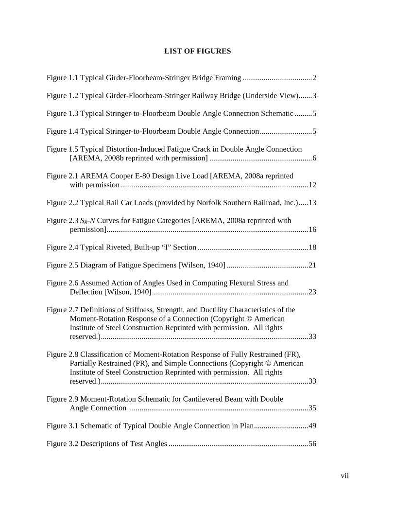
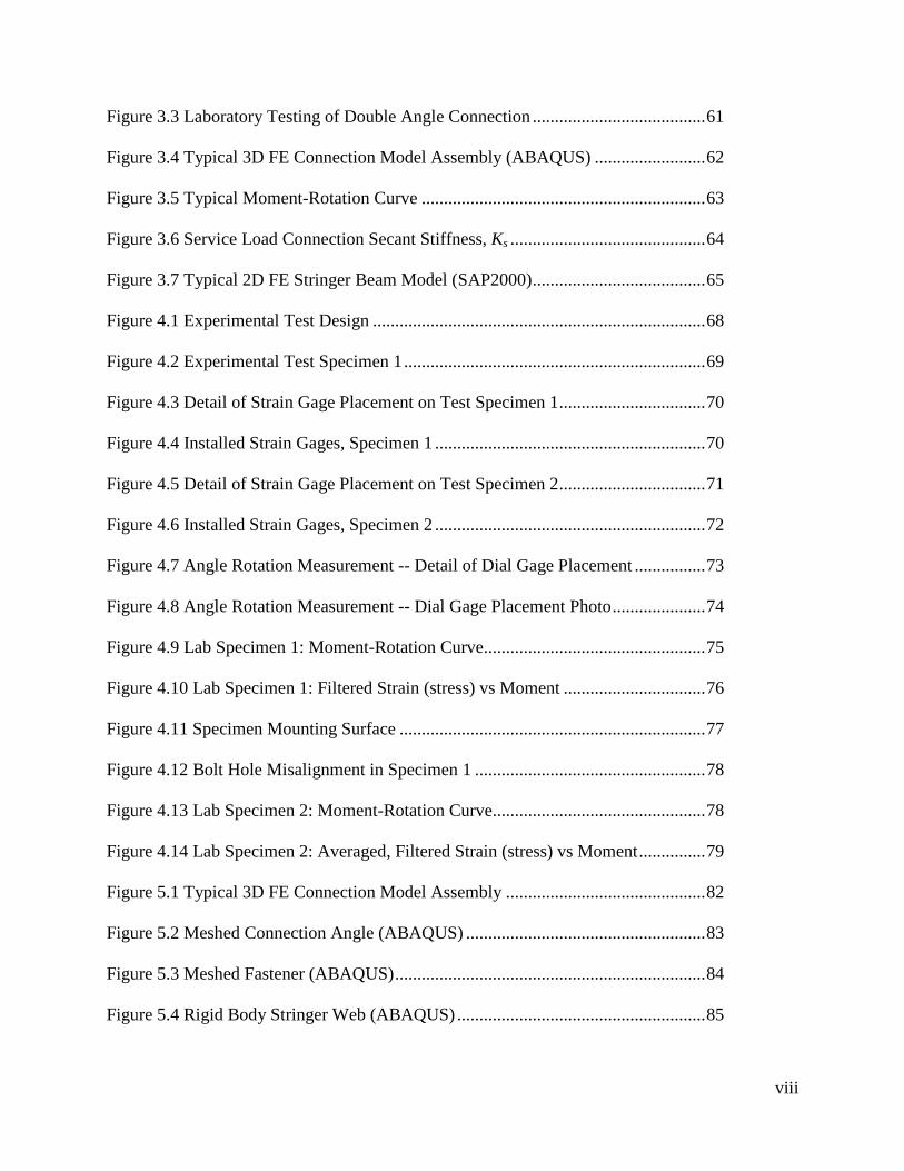
schematic is presented in Figure 1.3 and pictured in Figure 1.4. Additionally, a typical
distortion-induced fatigue crack is pictured in Figure 1.5.
5
Figure 1.3 Typical Stringer-to-Floorbeam Double Angle Connection Schematic
Figure 1.4 Typical Stringer-to-Floorbeam Double Angle Connection

6
Figure 1.5 Typical Distortion-Induced Fatigue Crack in Double Angle Connection
[AREMA, 2008b reprinted with permission]
1.2 Problem Statement
There has been little motivation to revisit Wilson’s 1940 study, because there have been no
reported fatal accidents or other catastrophes attributed to failure of these connections [Fisher et
al., 1990]. Additionally, these connections are not common in new construction so their design
is of little interest. However, if problems with in-service, double angle connections continue to
be evaluated on an individual, as-needed basis, then little is being done to address and identify
distortion-induced fatigue issues from a global perspective.
The intent of this research is to improve upon the fundamental approach of W.M.Wilson’s
1940 laboratory study with more precision and breadth of research by utilizing current analytical
tools and methodologies. Typical load-induced fatigue evaluation procedures are based on
computing nominal stresses by elementary mechanic methods for nominal loadings. These
stresses can then easily be compared to the permissible stress range for the required number of
cycles for the fatigue detail category under investigation. However, research has shown that

7
fatigue problems associated with distortion-induced stresses cannot be addressed in this way
because the stresses are not easily or uniquely computed [Roeder et al. 1998]. 3D finite element
analysis (FEA) is often used to evaluate the complicated behavior of distortion-induced fatigue
details. However, a detailed 3D distortion analysis of the stringer to floorbeam is not realistic for
most bridge inspections. A concise and readily applied stress prediction methodology is needed
to allow rapid and accurate evaluation of distortion-induced stresses for subsequent fatigue life
determination.
1.3 Scope of Research
An analytical, parametric study has been conducted to investigate the moment-rotation
behavior and distortion-induced stress concentrations in double angle connections. The study is
limited to riveted, double angle connections used to attach stringers-to-floorbeams in typical
railroad, girder-floorbeam-stringer bridges. Also, the fatigue load considered for this study is
limited to the 286,000 pound gross car weight (GCW) plus impact loading as defined for fatigue
evaluation in AREMA (2008a). In Chapter 2, a literature review identifies many parameters that
affect the behavior of double angle connections. An ideal goal for this research is to investigate
all possible parameters and ranges independently, however available time and resources do not
facilitate this. Therefore the scope of this study is limited by grouping parameters as primary
independent, secondary dependant, and constants. The primary independent parameters
considered in this study are:
• Gage distance of the outstanding leg
• Angle thickness
• Stringer length

8
• Angle depth
Reasonable primary parameter ranges have been determined from literature and also field
observation of railroad bridges from a previous study, “Condition Assessment of Short-line
Railroad Bridges in Pennsylvania” [Laman and Guyer, 2010]. Table 1.1 lists the primary
parameter ranges considered in this study.
Table 1.1 Range of Primary Parameters
Secondary, independent parameters are defined as some function of the above listed primary
parameters. They are:
• Rivet spacing
• Number of rivets
• Angle leg length
• Stringer stiffness
The secondary parameter formulation is discussed in detail in Chapter 3. Additionally, it is
known that the magnitude of initial tension within the rivet (obtained from the cooling and
shrinking of a hot driven rivet) and the friction between contacting surfaces are valid parameters
to consider. However, the scope of this study will be limited to non-variable values for rivet
Paramter
Gage Distance 2, 2.5, 3, 3.5, 4 inchesAngle Thickness 1/2, 5/8 inchesStringer Length 8, 10, 12, 14 feetAngle Depth 10, 11.5, 13, 14.5, 16 inches
Range of Values

9
clamping force and friction coefficient, µ as well as other non-variable parameters listed in Table
1.2.
Table 1.2 Non-Variable Parameters
1.4 Objectives
The objectives of this study are to determine the primary parameter effects on the moment-
rotation and maximum principal stress magnitude in double angle connections. Also, the
applicability and accuracy of empirical equations used to predict moment-rotation curves will be
investigated for double angle connections characterized by the range of parameters listed in
Table 1.1. The design rule proposed by Wilson (1940) will also be investigated to determine if it
is in fact suitable to preclude distortion-induced fatigue damage based on the results of this
parametric study. Lastly, a concise and readily applied stress prediction equation is proposed to
allow rapid and accurate evaluation of fatigue inducing stresses.
More concisely, the main objectives are:
1. Evaluate three empirical moment-rotation prediction equations for each unique
parametric study analysis case and compare with 3D FEA prediction. Determine which,
if any, empirical equations are reasonable to predict moment-rotation behavior.
Parameter
Material ConstantsRivet Clamping Force 15 kipsRivet Diameter 7/8 inches
Friction Coeficient, µFatigue Vehicle
Constant Value
286K GCW
0.5

10
2. For each of the 72 analysis cases, classify each connection according to the AISC
definitions: fully restrained (FR), partially restrained (PR), or simple.
3. Identify the effect that each primary parameter has on the load response behavior of the
double angle connection analysis cases.
4. Investigate design equation 1.1 and evaluate its effectiveness to preclude distortion-
induced fatigue damage.
5. Develop a stress prediction equation as a function of the primary study parameters to
facilitate quick and reliable fatigue life determination.

11
Chapter 2
LITERATURE REVIEW
2.1 Introduction
While not common in new construction, many older steel bridges are configured with double
angle connections to connect floor system members such as stringers and floorbeams. These
connections are assumed to rotate freely and transfer shear force only, however due to some
rotational stiffness, end moment is developed. Typically, the magnitude of the end moment is
small and can be neglected, therefore, a stringer is assumed to act as a simply supported beam.
This assumption is conservative for the design of the stringer because deflection and mid-span
moment is greater in a simple beam than a beam with some end fixity. However, by neglecting
the end moment, regardless of magnitude, distortion-induced stress in the connection angle from
stringer end rotation is also ignored. The accumulation of distortion-induced stress cycles over a
long service life can result in fatigue damage. The majority of in-service bridges with double
angle connections are found on railroads; many of the aging steel highway bridges have been
replaced by multi-girder or other configurations. A literature review has been conducted to
establish the state-of-the-art of distortion-induced fatigue in double angle connections with a
focus on railroad bridges.
This chapter presents railroad loads, both design and service, past and present with an
emphasis on cyclic loading resisted by double angle connections. A fundamental discussion of
fatigue is presented along with a summary of the legacy study from 1939 that the current
AREMA double angle connection design rule is based. The methods and results from several
other studies investigating distortion-induced fatigue in both highway and railroad bridges are

12
also discussed. Additionally, non-linear moment-rotation behavior of double angle connections
is introduced along with several published, empirical moment-rotation prediction equations.
This chapter concludes with a detailed discussion of finite element modeling techniques utilized
in previous research related to double angle connections.
2.2 Brief History of Bridge Loading
The American railroad system evolved and grew rapidly in the late 19th and early 20th
century. The size and weight of steam locomotives continuously increased through the 1930s,
thus bridges experienced heavier loads during this time. AREA continuously updated their
design Cooper E live load ratings to keep up with the increasing locomotive loads. In 1935, as
steam locomotives reached a maximum size, AREA established the design E-72 Cooper live
load. This live load was the design standard until 1969 when it was increased to E-80, shown in
Figure 2.1, where it remains today.
E80
-Loc
omot
ive
Figure 2.1 AREMA Cooper E-80 Design Live Load [AREMA, 2008a reprinted with permission]
The increase in 1969 was not due to a larger steam locomotive, as steam locomotives were
nearly completely phased out by lighter weight diesel electric locomotives in the early 1960s, but
rather due to the increase in the gross car weights (GCW) [Byers, 1992]. Prior to this time, the
40k
52k
52k
80k
80
k
80k
80
k
52k
52
k
40k
52k
52k
80k
80
k
80k
80
k
52k
52
k
60
60
60
96
108
60
72
60
96
96
60
60
60
108
60”
72
60
13
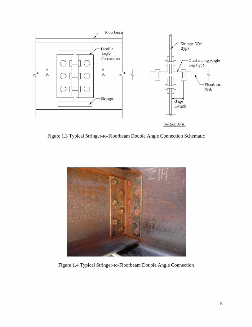
weight of train cars relative to the locomotive was small and, therefore, bridges only experienced
large design level service stresses under the load of the locomotive alone. In the 1960s, standard
GCW began to increase to 263,000 pounds and then to 286,000 pounds which are most common
at the present time. Some industrial railroads currently use 315,000 pound GCW equipment to
transport heavy commodities such as scrap metal. Figure 2.2 presents axle spacing and load for
typical 263, 000, 286,000 and 315,000 pound GCW equipment.
263,
000
lbs G
CW
286,
000
lbs G
CW
315,
000
lbs G
CW
Figure 2.2 Typical Rail Car Loads (provided by Norfolk Southern Railroad, Inc.)
As train car axle weights increased, bridges experienced larger service stress under the axle loads
from the entire train, rather than just the locomotive. Some bridge members, mainly short floor
system members, experience one complete load cycle from the passing of one train car truck.
65.75k 65.75k 65.75k 65.75k 65.75k
68” 235” 68” 80”
71.50k 71.50k
71.50k
71.50k
71.50k
68” 235” 68” 80”
78.75k 78.75k
78.75k
78.75k
78.75k
72” 368” 72” 76”

14
For a 100 car train, which is not uncommon, a floor stringer may undergo 200 load cycles, thus
raising concern about the fatigue life of the member and connections.
2.3 Fatigue Prone Detail: Double Angle Connection
The fabrication of steel bridges was accomplished with the use of rivets until the early 1960s
when high strength bolts were introduced. Furthermore, with the development of better
structural welding techniques in the late 1960s, the fabrication of welded bridge components also
became more common [Uppal, 2005]. Most in-service steel railroad bridges in Pennsylvania
date to the early 1900s [Laman et al., 2001], therefore, riveted fabrication was exclusively used
in their construction. Floor systems of bridges were typically constructed of longitudinal
stringers attached to transverse floor beams that were supported by the main bridge girders. The
stringer-to-floor beam connections were always accomplished with a double angle connection
[Fisher 1987]. The primary function of these connection angles is to transmit end shear from the
stringer to the floor beam but, because of the inherent stiffness, the angles are also subject to
flexural stresses due to the deformation of other portions of the structure.
Wilson and Coombe (1939) recognized that two actions contribute to secondary stresses in
connection angles. First, the stringers deflect vertically because of the wheel loads, and this
deflection rotates the end of the stringer and subjects the connection angles to a moment in the
plane of the stringer web. Second, in through-truss bridges, the bottom chord of the truss
changes in length due to a change in the chord stress resulting from the passage of a train. There
is no corresponding change in length of the stringer and, since the floor beam is connected to
both the chord and the stringer, an axial force is transmitted through the connection angle to the
stringer. The effect of the elongation of the bottom truss chord is to bend the outstanding leg of
15
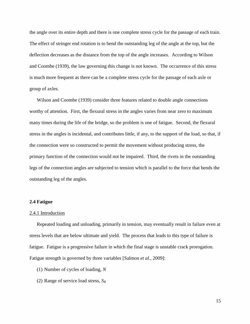
the angle over its entire depth and there is one complete stress cycle for the passage of each train.
The effect of stringer end rotation is to bend the outstanding leg of the angle at the top, but the
deflection decreases as the distance from the top of the angle increases. According to Wilson
and Coombe (1939), the law governing this change is not known. The occurrence of this stress
is much more frequent as there can be a complete stress cycle for the passage of each axle or
group of axles.
Wilson and Coombe (1939) consider three features related to double angle connections
worthy of attention. First, the flexural stress in the angles varies from near zero to maximum
many times during the life of the bridge, so the problem is one of fatigue. Second, the flexural
stress in the angles is incidental, and contributes little, if any, to the support of the load, so that, if
the connection were so constructed to permit the movement without producing stress, the
primary function of the connection would not be impaired. Third, the rivets in the outstanding
legs of the connection angles are subjected to tension which is parallel to the force that bends the
outstanding leg of the angles.
2.4 Fatigue
2.4.1 Introduction
Repeated loading and unloading, primarily in tension, may eventually result in failure even at
stress levels that are below ultimate and yield. The process that leads to this type of failure is
fatigue. Fatigue is a progressive failure in which the final stage is unstable crack prorogation.
Fatigue strength is governed by three variables [Salmon et al., 2009]:
(1) Number of cycles of loading, N
(2) Range of service load stress, SR

16
(3) Initial size of material flaw
Bridge design specifications, such as AREMA and AASHTO include multiple SR-N design
curves for specific detail categories. This family of curves is shown in Figure 2.3. Fatigue life is
calculated by first identifying the category of the detail under investigation. Next, the value of
service stress range is determined and the corresponding number of cycles until failure can be
determined from the SR-N relationship. Finally, fatigue life expressed in time can be determined
if the loading frequency is known.
The stress magnitude at which the diagram becomes horizontal is referred to as the endurance
limit or sometimes called the threshold stress, constant amplitude fatigue limit or just fatigue
limit. This limit is considered the maximum stress the material can endure for a presumably
infinite number of cycles without failure.
Figure 2.3 SR-N Curves for Fatigue Categories [AREMA, 2008a reprinted with permission]

17
For variable amplitude loading, the Palmgren-Miner fatigue rule is often used to assess the
cumulative fatigue damage. The Palmgren-Miner rule quantifies the cumulative fatigue damage
as a summation of incremental damage that occurs at various stress amplitudes. When
examining a more complex variable stress spectrum, a rainflow-counting algorithm can be
utilized to develop a histogram representing the number of cycles occurring at given stress
amplitudes. Once the stress spectrum is represented in a histogram, the Palmgren-Miner rule can
be evaluated to determine fatigue damage. The scope of the research presented in this thesis is
limited to live loading from a 286,000 lb GCW only. Therefore a constant amplitude stress is
assumed and the Palmgren-Minor rule and the rainflow-counting algorithm will not be further
discussed.
2.4.2 Fatigue Studies
The fatigue damage that is expected to have accumulated in riveted steel bridges is of
concern because many of these bridges were put into service at the beginning of the 20th century.
Due to the long service life, questions of safety arise because of increased traffic and axle loads,
deteriorating components and the accumulation of large numbers of load cycles. In addition to
riveted member-to-member connections, such as double angles, the members themselves are
built-up from plates and angles and riveted together as pictured in Figure 2.4. For example, a
typical “I” section is constructed from a web-plate riveted to flange angles. Flange cover plates
are then riveted to the flange angles to increase the thickness of the flange. Therefore, it is
important to recognize that “riveted connection” can refer to member-to-member connections but
also internal built-up member connections. Many studies and experiments have been conducted
to investigate the fatigue strength in riveted bridge members.

18
Figure 2.4 Typical Riveted, Built-up “I” Section
Fisher et al. (1990) compiled and examined experimental data from more than 1200 previous
fatigue tests that were performed in the United State and Europe between 1934 and 1987. A
large number of these tests were conducted on laboratory specimens, most of which were simple
riveted shear splices. In the review, primary focus was given to the cyclic stress range as the
main parameter influencing fatigue life but two other major variables affecting the fatigue
resistance are rivet clamping force and the rivet bearing ratio. The fatigue data associated with
the testing of these simple, riveted, shear splice specimens was superimposed on the S-N lines of
fatigue strength categories C, D, and E. Nearly all tests results exceed the fatigue strength of
category D. Fisher et al. (1987,1990) also reviewed fatigue test data from full-scale riveted
bridge members. These tests, while not very extensive, were performed on different types of
members ranging from riveted truss members to riveted built-up stringer and girders to rolled
sections with riveted cover plates. The fatigue tests of full-scale girders, performed by Fisher at

19
Lehigh University, were conducted at ambient room temperature and at reduced temperatures as
low as -100°F to simulate the lowest levels of fracture resistance likely to exist. The principal
findings from studies carried out on large-scale riveted member reveal that, like the small-scale
specimens, category D provides a reasonable lower-bound fatigue strength limit. Also, the type
of riveted member and detail does not appear to be a significant factor as they all provided
comparable fatigue resistance. The tests also show that relatively large fatigue cracks can be
sustained at ambient and reduced temperatures prior to fracture of a component. These tests also
indicate that failure of a single component did not result in an immediate loss of load-carrying
capability. This demonstrates that such members are inherently redundant with respect to
fracture and are capable of redistributing the forces in the cracked member. AREMA (2008a)
cites Fisher, 1990 in the commentary as the basis for adopting category D fatigue resistance for
riveted members.
DiBattista et al. (1998) also examined the fatigue testing of full-scale riveted bridge
specimens that were taken from a variety of sources, most from structures that had been in
service. These test data examined by DiBattista et al. (1998) includes that of the full-scale tests
investigated by Fisher et al. (1990) and also a number of additional tests performed in the mid-
1990s. This collection of fatigue data was then compared to design fatigue rules published by
AASHTO, AREMA (formerly AREA), Eurocode, and British Standard 5400. The conclusion is
that the most suitable fatigue life category for riveted shear splices is that of category D as
prescribed by AREMA.
The results from numerous fatigue tests as provided by Fisher et al. (1987, 1990) and
DiBattista et al. (1998) are primarily those of load-induced fatigue from in-plane bending or
direct tension, however, literature suggests that the most common types of fatigue damage are

20
due to distortion effects in end connections [Fisher et al. 1987, Depiero et al. 2002, Imam et al.
2007, Al-Emrani et al. 2003, Fisher et al. 1990]. Fisher et al. (1990) comment that “limited test
on end connection angles indicated that their fatigue strength was in agreement with category A
for base metal.” No other specific information is provided about these limited tests other than
bending stresses were caused by end rotation of the stringer and they were estimated from a
simple flexural model that assumed double curvature in the outstanding leg of the angle.
Presumably Fisher is referring to the nine tests conducted by Wilson and Coombe (1939) as this
information is consistent with Wilson’s study. In 1939, Wilson and Coombe tested 9 laboratory
specimens, each representing a short length of the riveted, double angle connection between the
stringer and a floor beam to which they are connected. Three series of three specimens each
were constructed of two central plates, four filler plates, four angles, and a spacer as shown in
Figure 2.5. The action of the testing machine was to subject the specimen to an axial force,
parallel to the longitudinal axis of the stringer that varied from zero to a maximum tension at a
rate of 180 cycles per minute. This applied force represents “the same kind of stress cycle as the
connection angles of through truss bridges are subjected to as a result of the change in stress in
the chord that occurs with each passage of a train. Moreover, this action approximates closely
the action to which the tops of the connection angles of a bridge are subjected with the passage
of each truck because of the deflection of the stringers.” [Wilson and Coombe 1939].
Mechanical strain gages were attached to the ends of the angles to measure deflection of the
angles as the load was applied. The tension rivets were also instrumented with strain measuring
devices. Wilson and Coombe acknowledge that results from complex test specimens such as
these can be erratic and many tests at varying stresses are necessary to define a curve describing
the relationship between stress and number of cycles to failure.

21
Figure 2.5 Diagram of Fatigue Specimens [Wilson, 1940]

22
However, due to limited funding, the results of only nine tests were normalized such that the
quantified fatigue strength, F is defined as the maximum stress in the stress cycle, varying from
zero to maximum, which will cause failure at 2,000,000 repetitions. This is given by the
following empirical formula:
10.0
10.0
2000000SNF = (2.1)
where S and N represent the stress and number of cycles for failure respectively for a particular
test. The results of all nine tests are presented in Table 2.1.
Table 2.1 Fatigue Strength of Connection Angles (Wilson, 1939-reproduced with permission)
The flexural stress was computed from stain measurements and the assumption that the
outstanding leg of the angle remains fixed under the tension rivet and at the fillet. Based on
At Beginning of Test
Near End of Test
At Beginning of Test
Near End of Test
Rivet Angle
1 2 3 4 5 6 7 8 9 10 11C1-1 18,000 46,200 6,200 12,300 0.0088 0.0218 302,000 15,300 39,250+ RivetC1-2 15,000 39,000 4,520 1,700 0.0054 0.0068 2,305,000 15,200+ 39,560 AngleC1-3 16,000 41,500 3,670 2,260 0.0069 0.0081 3,245,000 16,800+ 43,560+ No Failure
C2-1 30,000 38,700 7,200 ----- 0.0248 0.0374 12,200 18,000 23,240+ RivetC2-2 20,000 25,800 1,680 5,280 0.0024 0.0031 2,961,200 20,800 26,830+ RivetC2-3 25,000 32,300 1,200 3,600 0.0044 0.0077 267,700 20,450 26,410+ Rivet
C3-1 7,420 73,200 5,600 ----- 0.1096 0.112 89,200 5,667+ 53,630 Angle C3-2 5,920 58,800 2,270 1,860 0.0751 0.0812 25,900 4,825+ 48,530 AngleC3-3 4,250 42,000 270 350 0.0498 0.0491 3,119,400 4,445+ 43,900+ No Failure
* For rivet that failed, or average for all rivets if none failedł Average from gage lines 11 and 12 for the two ends, four gage lines in all
+ Fatigure strength equals or exceeds this value; part did not fail¶ The flexural stress was computed from the total load on the basis that the action of the angles was indicated in Fig 2.6
Fatigue Strength of Connection AnglesStress cycle, zero to tension
Specimen Number
Maximum Load in Terms of Average
Tension in the Rivets
lb. per sq. in.
Flexural Stress in Angle
lb. per sq. in 
Variation of Tension in Rivet During Cycle
lb. per sq. in.*
Deflection of Two Angles During Cycle in Inches ł
Number of Cycles for
Failure
Fatigue Strength
Part That Failed

23
these boundary conditions, the outstanding angle leg experiences double curvature with an
inflection point occurring at half the gage distance as shown in Figure 2.6. It can be observed
from columns 9 and 10 of Table 2.1 that computed fatigue strength of the rivets is approximately
15 ksi and fatigue strength of the angle varies from about 40 to 53 ksi. Wilson and Coombe
(1939) recognize that the yield strength of a rolled plate is only 35 ksi, therefore, it is realized
that “the method of computing the flexural stress in the outstanding legs of the angles give values
that are probably somewhat greater than the true value.” [Wilson and Coombe 1939].
Figure 2.6 Assumed Action of Angles Used in Computing Flexural Stress and Deflection [Wilson, 1940]
Wilson and Coombe summarize their study by recognizing that because the number of tests
was small, results are limited to statements relative to the action of the particular specimens
tested. The results obtained were as follows:

24
(1) The deformation of the angle did not differ greatly from the fixed-fixed boundary
condition assumed for the outstanding leg.
(2) The average fatigue strength for the tension rivets was 16 ksi and 20 ksi for the series C1
and C2 specimens respectively.
(3) The average fatigue strength in flexure of the outstanding leg of the angles for series C3
was of the order of 50 ksi.
(4) When specimens were loaded to their fatigue strength, the longitudinal movement of one
stringer relative to the other was 0.0069, 0.0024, and 0.063 inches for the specimens of
series C1, C2, and C3 respectively.
Fisher et al. (1990) discuss distortion-induced fatigue based on their own field observations
of riveted structures. They conclude that the occurrence of fatigue cracks in riveted structures
has frequently been at member end connections. These cracks in end connection angles are due
to bending stresses that were not accounted for in the original design. Additionally, cracks have
been observed not only at the top, tension side, of the angle but also at the bottom in the
compression side. Many of these cracks propagate slowly and can be arrested by drilling a hole
at the crack tip, however, Fisher et al. (1990) reported the complete failure of an end connection
when the cause of the crack growth was not corrected. Because distortion-induced cracks
typically originate near the fillet of the connection angle, the fatigue strength generally
corresponds to category A for base metal fatigue resistance. However, it is difficult to accurately
predict these stresses in actual structures using normal analysis models. Additional studies are
needed on distortion of connection angles so that rational connection details can be developed
[Fisher et al., 1990].

25
2.5 Design of Connection Angles
In 1940, Wilson furthered his study on double angle stringer connections to include design
recommendations to ensure adequate flexibility in the angle such that they are not overstressed
by distortion induced stresses. Because the floor system of a bridge is statically indeterminate
due to connections of unknown stiffness, Wilson had to make use of several simplifying
assumptions. Listed below are the assumptions and relationship Wilson used.
(1) The stress-deflection relationship for the outstanding angle leg as derived from the 1939
fatigue tests was used.
(2) Elastic behavior is assumed.
(3) The center of rotation is assumed to be at mid-depth of the stringer.
(4) Fixed boundary condition is assumed for the outstanding angle leg.
(5) Flange stress in the stringer is calculated based on live load plus impact.
(6) The axial deformation for the effect of both chord elongation and stringer rotation was
computed by Hooke’s Law.
Based on these deformations and the stress-deflection relationships previously determined,
the stresses in the angle associated with its stiffness could then be determined. Realizing that the
deflection of the outstanding leg varies directly with the stringer length, L, and angle thickness, t,
and inversely to the square of the gage, g, Wilson proposed equation 1.1. This design rule was
adopted by AREA and is currently the published design standard with respect to distortion
stresses [AREMA, 2008a].
In addition to satisfying the design rule in equation 1.1, the current design specification
[AREMA, 2008a] specifies that welding shall not be used to connect the flexing (outstanding)
angle leg and that the flexing leg shall not be less than 4 inches in width and ½ inch thick.

26
Based on the same reasoning and criteria used by Wilson, a constant of proportionality, K=
12 was suggested by Fisher (1987) for highway bridge structures. This suggestion would result
in an angle with increased stiffness.
2.6 Bridge Field and Case Studies of Double Angle Connection
2.6.1 Highway Bridges
The Winchester Bridge, carrying Interstate 5 in Oregon is a riveted steel deck truss structure
that has required extensive replacement of connection details because of fatigue crack growth.
The cracks, up to 4 inches in length, have been discovered in the clip angles in the stringers-to-
floor beams connections. The cracks originated in the top of the outstanding leg of the angle,
near the fillet. DePiero et al. (2002) used finite element (FE) modeling to characterize the
behavior of the structure on both a global and local level.
Global FE models were developed to determine the distribution of live loads on the stringers.
To quantify the live loading and to assist in validating the analysis, field testing was also
performed on the bridge. The bridge was instrumented with strain gages at various locations to
collect load response data under normal traffic and under controlled loading. The measured
stresses were lower than those calculated by the global FE model. This discrepancy is most
likely attributed to the composite interaction between the reinforced concrete deck and steel
superstructure which was not accounted for in the FE model.
Local 2D and 3D FE models were developed to characterize the clip angle connection.
These models were loaded with stress levels determined from the global FE model. Both 2D and
3D models predict the location of maximum stress to be located near the root of the angle fillet.
The 3D model more accurately predicted deflections due to better representation of actual

27
boundary conditions that exist at the connection interfaces. Stress levels in the clip angles, as
determined from the 3D FE model, range from 8.5 ksi to about 27 ksi, depending on the location
in the bridge structure.
DePiero et al. (2002) concluded that while the stress ranges in their model are conservative,
the analysis performed indicated that the connection details are prone to distortion-induced
fatigue. The 3D stress analysis of the connection shows that maximum principal stresses are
localized and that crack growth beyond this local area might result in lower stress ranges and
crack self-arrest.
Of additional interest, according to Wilson’s design rule (eqn 1.1), the required gage distance
for the top one-third of the outstanding leg of stringer connections on the Winchester Bridge
should be greater than 3 inches. DePiero et al. (2002) indicate a gage distance of only 1.5
inches.
Roeder et al. (1998) investigated the fatigue characteristics of two riveted highway bridges
that carry Interstate 5 in Washington State, the Lewis River Bridge and the Toutle River Bridge.
The Lewis River Bridge is a three-span, continuous, riveted truss that is 810 feet in total length.
The Toutle River Bridge is a single span, 300 foot, riveted tied arch bridge. Computer models of
the two structures were developed with both static and dynamic analysis performed.
Instrumentation was installed on the two bridges and controlled load and weigh-in-motion tests
were performed with trucks of known weight and geometry traveling at known speed. These
results were used to evaluate the global bridge response and also calibrate the computer models.
Observations revealed that, due to the flexibility of these structures, distortion-induced fatigue
stresses are of major concern, especially in floor members. These fatigue causing stresses

28
develop because of the rotational stiffness in the end connections of stringers and floor beams.
Roeder et al. (1998) modeled these partially restrained connections with springs having a
rotational stiffness computed from measured end rotations under known loads. It was concluded
that “elimination of end rotational restraint of the stringer-to-floor beam connections could
significantly increase the fatigue life of these connections.” [Roeder et al. 1998]. This could be
accomplished by “knocking out some of the top rivets and adding a stiffened seat.” [Roeder et al.
1998]. This retrofit would preserve shear capacity of the connection while providing increased
joint flexibility, thus reducing stress concentrations. However, increased joint flexibility will
increase deflections in the structure that could lead to more rapid deterioration of other
components. Removal of rivets has been reported as a damage limitation method that has
sometimes been successful, but, in other cases has not been, therefore, it is seldom used [Roeder
et al. 2005].
2.6.2 Railway Bridges
Philbriek et al. (1995) investigated the behavior of two girder-floorbeam-stringer railroad
bridges to determine a better approach to fatigue assessment. Both bridges, built in the early
1900s are of similar construction and both appeared to be in good condition with no evidence of
major repairs or retrofitting. These bridges were instrumented and measurements of strain and
deflection were recorded during the crossing of a train. The field measurements were used to
calibrate a parametric study of the modeling of each bridge. Among the interests of this study
were the rigidity of member connections and its effect on structural continuity and the
distribution of axle loads through the track structure. A computer model was developed for the
bridge superstructure, utilizing material and geometric properties of the members. Moments
29
calculated from field data taken near mid-span of the stringers displayed sign reversal with
significant negative moments occurring when axle loads were on adjacent stringer spans. The
stringer-to-floorbeam and floorbeam-to-girder connections were therefore assumed to be fixed
since it was evident there was significant structural continuity of the bridge floor system. Fixed
connection stiffness of 4EI/L was assigned to the model. The analysis provided results that
displayed structural continuity levels similar to those found from field data.
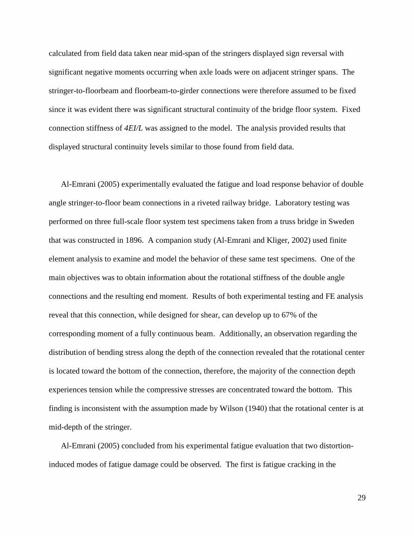
Al-Emrani (2005) experimentally evaluated the fatigue and load response behavior of double
angle stringer-to-floor beam connections in a riveted railway bridge. Laboratory testing was
performed on three full-scale floor system test specimens taken from a truss bridge in Sweden
that was constructed in 1896. A companion study (Al-Emrani and Kliger, 2002) used finite
element analysis to examine and model the behavior of these same test specimens. One of the
main objectives was to obtain information about the rotational stiffness of the double angle
connections and the resulting end moment. Results of both experimental testing and FE analysis
reveal that this connection, while designed for shear, can develop up to 67% of the
corresponding moment of a fully continuous beam. Additionally, an observation regarding the
distribution of bending stress along the depth of the connection revealed that the rotational center
is located toward the bottom of the connection, therefore, the majority of the connection depth
experiences tension while the compressive stresses are concentrated toward the bottom. This
finding is inconsistent with the assumption made by Wilson (1940) that the rotational center is at
mid-depth of the stringer.
Al-Emrani (2005) concluded from his experimental fatigue evaluation that two distortion-
induced modes of fatigue damage could be observed. The first is fatigue cracking in the

30
outstanding leg of the connection angles. These cracks initiated near the fillet at the top of the
angle and propagated slowly down the length. The other damage mode was the cracking of
tension rivets due to prying action of the angle. For both cases, fatigue damage development was
associated with a gradual reduction in rotational stiffness of the connection. As the number of
load cycles continued to increase, it was observed in all specimens that cracks eventually self-
arrested. Also, when up to 40% of the connection angles had cracked or when 8 of the 10 rivets
in the connection had fractured, the connections were still able to transfer considerable shear
force, yet with substantial yielding and large deformation.
Al-Emrani and Kliger (2002), concluded from the FE analysis that the flexibility of the
outstanding legs of the connections angles has a major influence on the response of the double
angle connection. In particular, the gage distance between the tension rivets and the fillet was
found to play a dominant role in the behavior of these connections. Also, the magnitude of the
clamping force in the rivet had only a marginal effect on the rotational stiffness of the connection
and the flexural stresses in the angles were virtually not affected by the rivet clamping force.
However, the resulting stress ranges in the rivets of the connection were greatly influenced by
the clamping force magnitude. Rivet bending due to prying action, together with stress a
concentration present at the junction between the rivet shank and its head was found to be the
major mechanism behind rivet fracture. This provides evidence that a fixed boundary condition
for the angle under the rivet head is not necessarily valid.
Imam et al. (2007) investigated riveted railway bridge connections for fatigue evaluation by
numerical modeling. A stringer-to-floor beam connection in a typical short-span, riveted, plate
girder bridge was modeled using ABAQUS finite element code. This connection model was
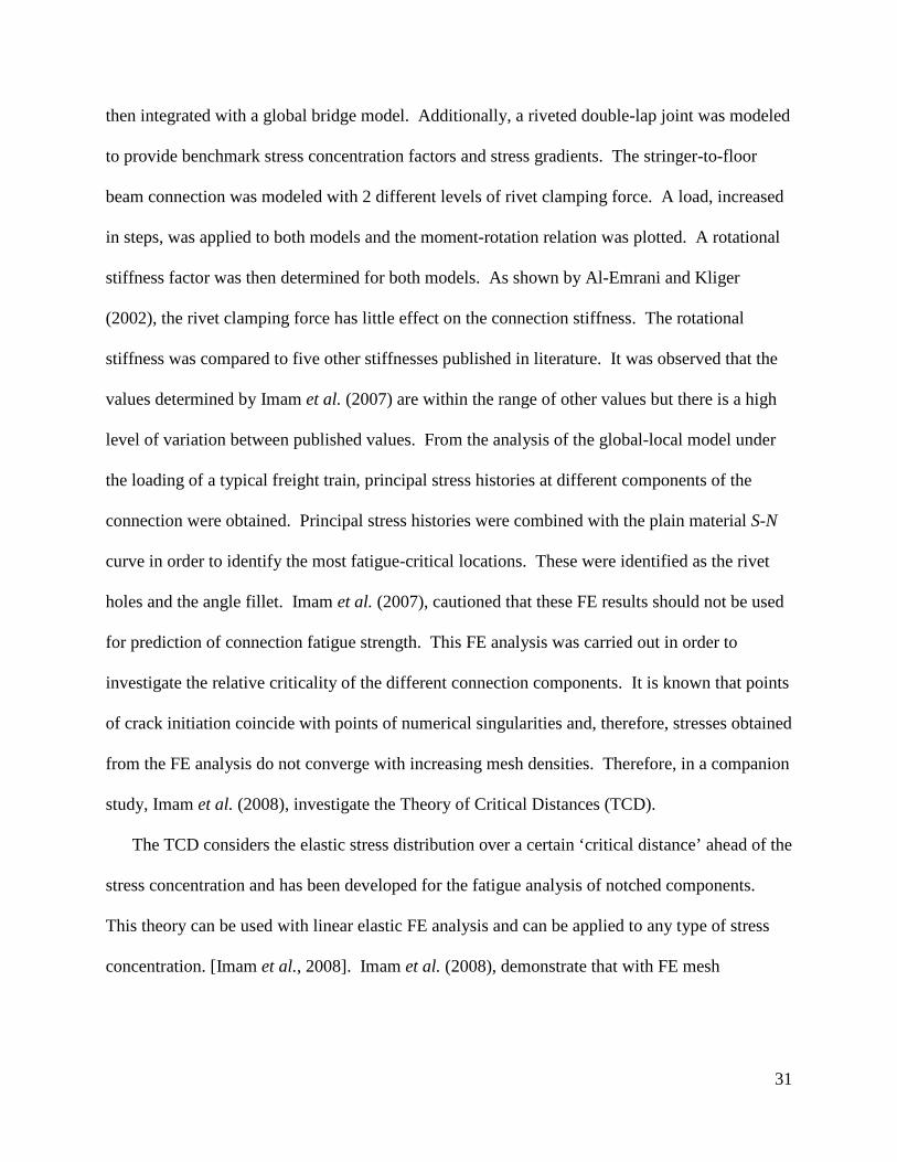
31
then integrated with a global bridge model. Additionally, a riveted double-lap joint was modeled
to provide benchmark stress concentration factors and stress gradients. The stringer-to-floor
beam connection was modeled with 2 different levels of rivet clamping force. A load, increased
in steps, was applied to both models and the moment-rotation relation was plotted. A rotational
stiffness factor was then determined for both models. As shown by Al-Emrani and Kliger
(2002), the rivet clamping force has little effect on the connection stiffness. The rotational
stiffness was compared to five other stiffnesses published in literature. It was observed that the
values determined by Imam et al. (2007) are within the range of other values but there is a high
level of variation between published values. From the analysis of the global-local model under
the loading of a typical freight train, principal stress histories at different components of the
connection were obtained. Principal stress histories were combined with the plain material S-N
curve in order to identify the most fatigue-critical locations. These were identified as the rivet
holes and the angle fillet. Imam et al. (2007), cautioned that these FE results should not be used
for prediction of connection fatigue strength. This FE analysis was carried out in order to
investigate the relative criticality of the different connection components. It is known that points
of crack initiation coincide with points of numerical singularities and, therefore, stresses obtained
from the FE analysis do not converge with increasing mesh densities. Therefore, in a companion
study, Imam et al. (2008), investigate the Theory of Critical Distances (TCD).
The TCD considers the elastic stress distribution over a certain ‘critical distance’ ahead of the
stress concentration and has been developed for the fatigue analysis of notched components.
This theory can be used with linear elastic FE analysis and can be applied to any type of stress
concentration. [Imam et al., 2008]. Imam et al. (2008), demonstrate that with FE mesh

32
refinement, reasonable convergence is achieved through the use of TCD and reasonable
predictions for remaining fatigue lives can be made.
2.7 Moment – Rotation Behavior of Double Angle Connections
Steel structures are generally designed by assuming member joints are either pinned (simple)
or rigid (fully restrained) but in actuality, the behavior of all joints is somewhere in between.
Therefore, the American Institute for Steel Construction (AISC) provides three different
connection classifications: simple, fully restrained (FR), and partially restrained (PR). The basic
assumption made in classifying connections is that the most important behavioral characteristics
of the connection can be modeled by a moment-rotation (M-θ) curve.
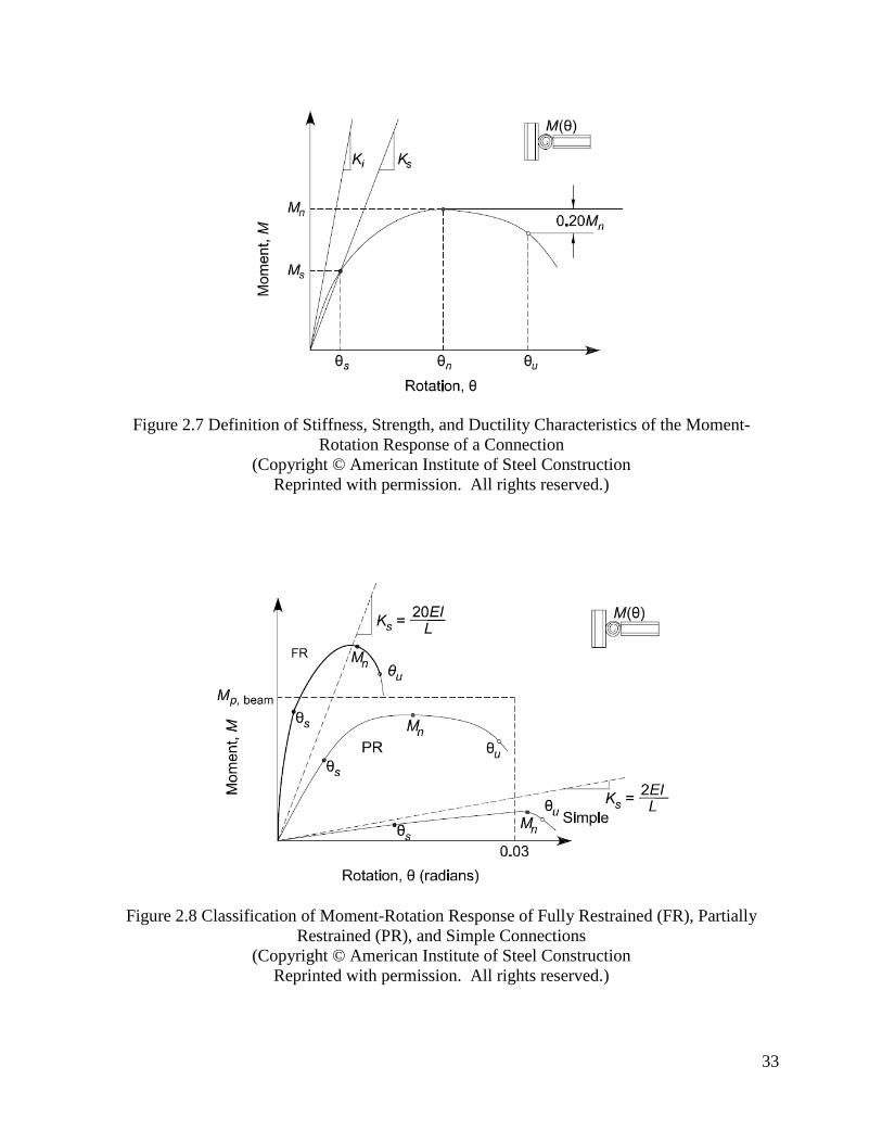
2.7.1 Connection Stiffness, K
The initial connection stiffness, Ki is the slope of the tangent at initial loading. It is seen from
Figure 2.7 that due to the non-linear behavior of the M-θ curve, Ki does not adequately
characterize the connection at service levels. Therefore the secant stiffness, Ks at service loads is
taken as an index property of connection stiffness and is defined by equation 2.2 where Ms and θs
are the moment and rotation at service level respectively.
s
ss
MK
θ= (2.2)
The definition provided by AISC for FR, PR, and simple connection classification is shown in
Figure 2.8 in terms of Ks, length of the beam, L and bending rigidity, EI. By this definition, the
stiffness of the connection is meaningful only when compared to the stiffness of the connected
member. Recall that Philbriek et al. (1995) considered 4EI/L for fixed connection stiffness.
33
Figure 2.7 Definition of Stiffness, Strength, and Ductility Characteristics of the Moment-Rotation Response of a Connection
(Copyright © American Institute of Steel Construction Reprinted with permission. All rights reserved.)
Figure 2.8 Classification of Moment-Rotation Response of Fully Restrained (FR), Partially Restrained (PR), and Simple Connections
(Copyright © American Institute of Steel Construction Reprinted with permission. All rights reserved.)

34
2.7.2 Connection Strength
The strength of a connection is the maximum moment, Mn that it is capable of carrying as
seen in Figure 2.8. The strength can be determined by analytical models or experimentally. If
the moment-rotation response does not show a maximum peak value then the strength can be
taken as the moment corresponding to a rotation of 0.02 radians. Connections that transmit less
than 20% of the fully plastic moment of the beam, Mp at a rotation of 0.02 radians may be
considered to have no flexural strength for design [AISC, 2005].
2.7.3 Connection Ductility
If the beam strength exceeds the connection strength, as is often the case with typical double
angle connections, then deformations can concentrate in the connection. Ductility requirements
for a connection will depend on the particular application. In the case with most double angle
connections, the connecting elements must be configured so that flexing of that connecting
element accommodates the simple beam end rotation. As seen in Figure 2.7, the rotational
capacity, θu can be defined as the value of connection rotation at the point where either (a) the
resisting strength of the connection had dropped to 0.8Mn or (b) the connection has deformed
beyond 0.03 radians [AISC, 2005].
2.7.4 Derivation of Moment-Rotation Curves
Historically, M-θ curves for a connection have typically been derived from experimental
testing similar to the schematic presented in Figure 2.9. Over the years, data from many of these
tests have been collected into various databases [Chen, 2000].

35
Figure 2.9 Moment-Rotation Schematic for Cantilevered Beam with Double Angle Connection
From this collection of data, many different equations for the entire M-θ curve for different
connection types have been proposed. It is recognized however, that numerous variables, such
as material properties and torque in the bolts are generally poorly documented, thus many of the
M-θ curves and equations derived from these databases may not be reliable. Also, the scope for
much of the research in double angle connections is limited to beam-column connections typical
of steel building construction. In general, the connections and member are lighter than those
typical of bridge construction. Care must be exercised when using derived equations not to
extrapolate to conditions outside the scope of data used to develop the model [Tamboli, 2010].
A few analytical models, believed to be the most accepted, are presented here.
In 1975, Frye and Morris developed an empirical model which is based on an odd power
polynomial representation of the M-θ curve shown in equation 2.3 where K is a parameter
depending on the geometrical and mechanical properties of the connection and C1, C2, and C3 are
curve fitting constants.
53
321 )()()( KMCKMCKMC ++=θ (2.3)

36
The Frye-Morris model was based on a procedure formulated by Sommer in 1969 which used
the method of least squares to determine the constants of the polynomial. [Chen, 2000].
Richard and Abbott developed a three parameter power model in 1975 shown in equation 2.4
to mathematically represent the M-θ curve. It was concluded that the three parameter power
model could replace the experimental test data in describing adequately the connection M-θ
curve behavior for practical use. [Chen, 2000].
nn
u
ki
ki
MR
RM /1
1
+
=θ
θ (2.4)
where the modeling parameters are defined as:
Mu = ultimate moment capacity
n = shape parameter
Rki = initial connection stiffness
The modeling parameters for equation 2.4 can be defined by experimental test data points if it
exists for the connection under consideration. Alternatively, Kishi and Chen (1990) as well as
Attiogbe and Morris (1991) have proposed models to predict the parameters for double angle
connections for use in the Richard and Abbott equation above.
Kishi and Chen (1990) developed a semi-analytical procedure to predict parameters for use
in equation 2.5. The initial connection stiffness, Rki is represented by equation 2.5.
)sinh()cosh()()cosh(
3
3
αβαβαβαβα−
= aki
tGR (2.5)
where:
G = shear modulus of connection angle
ta = thickness of the angle

37
α = 4.2967 when Poisson’s ratio is 0.3
β = g1/lp (2.6)
g1 = gc – ka – w/2 (2.7)
lp = length of the angle
gc = gage distance of the outstanding angle leg
ka = distance from the angle heel to toe of the fillet
w = width of the fastener’s nut
The ultimate moment capacity, Mu is given by equation 2.8 below.
+
= 2
62
22 p
aypu
u l
tfV
M (2.8)
fy = yield strength of angle
Vpu is determined by the following relationship
1224
=
−+
a
pu
ya
ac
a
pu
y tV
ftkg
tV
f (2.9)
Finally with Mu and Rki known, the shape parameter, n can be computed by the following
relationship proposed by Liew [Faella et al., 2000] in equation 2.10.
60.0952.3log322.1 10 ≥+=ki
u
RM
n (2.10)
The M-θ curves created using the Kishi and Chen parameters in the Richard and Abbott equation
2.4 were compared with test data from a connection databank at Purdue University. Kishi and
Chen (1990) conclude that the power model agrees rather well with the experimental results.
Attiogbe and Morris (1991) have proposed an empirical model for predicting the M-θ
response for a given connection topology derived by a least squares curve fitting procedure from
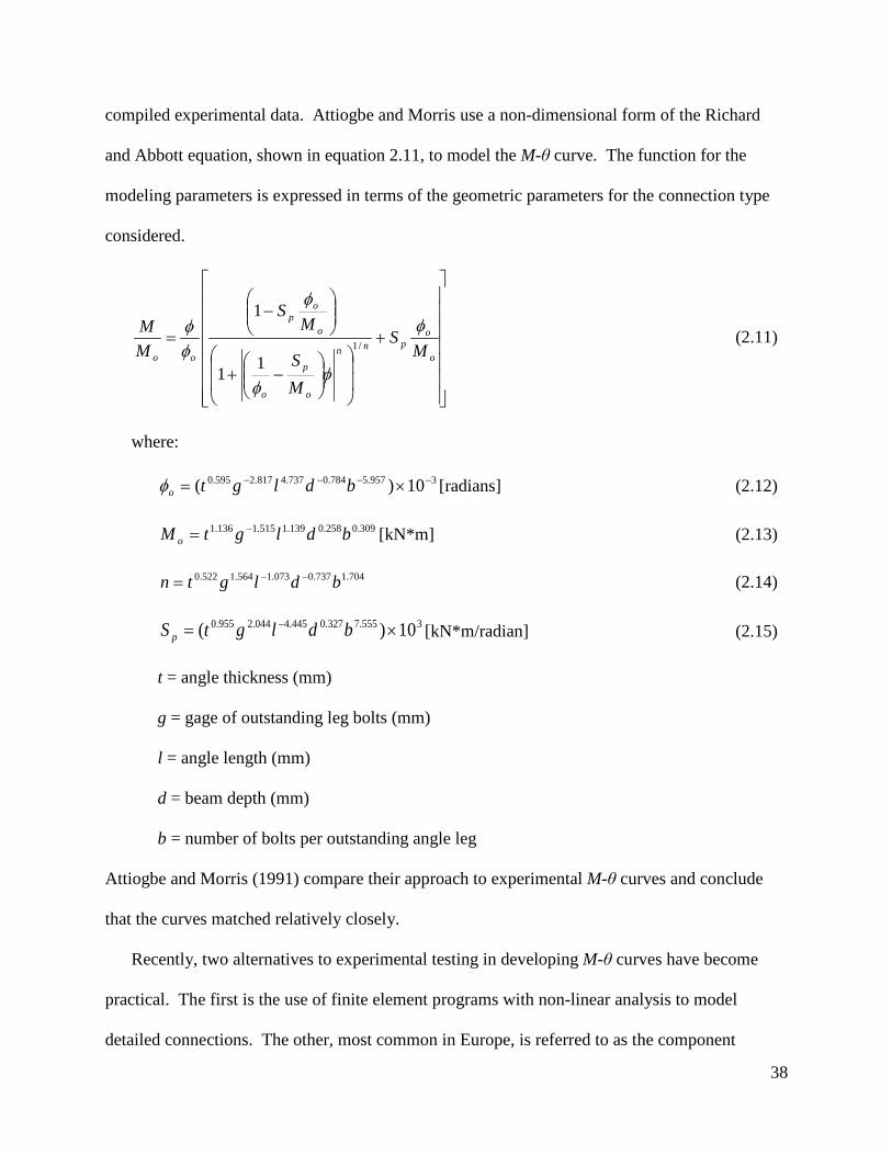
38
compiled experimental data. Attiogbe and Morris use a non-dimensional form of the Richard
and Abbott equation, shown in equation 2.11, to model the M-θ curve. The function for the
modeling parameters is expressed in terms of the geometric parameters for the connection type
considered.
+
−+
−
=o
opnn
o
p
o
o
op
oo MS
MS
MS
MM φ
φφ
φ
φφ
/1
11
1 (2.11)
where:
3957.5784.0737.4817.2595.0 10)( −−−− ×= bdlgtoφ [radians] (2.12)
309.0258.0139.1515.1136.1 bdlgtM o−= [kN*m] (2.13)
704.1737.0073.1564.1522.0 bdlgtn −−= (2.14)
3555.7327.0445.4044.2955.0 10)( ×= − bdlgtS p [kN*m/radian] (2.15)
t = angle thickness (mm)
g = gage of outstanding leg bolts (mm)
l = angle length (mm)
d = beam depth (mm)
b = number of bolts per outstanding angle leg
Attiogbe and Morris (1991) compare their approach to experimental M-θ curves and conclude
that the curves matched relatively closely.
Recently, two alternatives to experimental testing in developing M-θ curves have become
practical. The first is the use of finite element programs with non-linear analysis to model
detailed connections. The other, most common in Europe, is referred to as the component

39
approach. In this case, each deformation mechanism in the connection is identified and its
behavior is quantified by either a linear or nonlinear spring. These springs are arranged in series
or parallel and the overall M-θ curve can be derived with the aid of simple computer programs.
[Faella et al., 2000]. The component approach is outside the scope of this thesis and will not be
discussed further.
2.8 Finite Element Modeling of Double Angle Connections
2.8.1 Introduction
Finite element programs such as SAP2000, ANSYS, and ABAQUS are common analysis
tools used by researchers to evaluate various structural problems that otherwise would have to be
performed in the field or laboratory and would presumably require extensive resources. Earlier
in this chapter, several research studies were discussed that used finite element analysis to
investigate the behavior of double angle connections. This section will revisit some of those
studies and review others with an emphasis on FE modeling and techniques used to accurately
model double angle connection behavior.
2.8.2 Finite Element Modeling
DePiero et al. (2002) created a 3D FE model of a double angle stringer-to-floorbeam
connection for the Winchester Bridge carrying Interstate 5 in Oregon. The objective of the
model was to accurately determine deflection and stress in the connection angle subject to
loading from the AASHTO fatigue truck. The angle, stringer, and floorbeam were created and
meshed as separate parts using hexahedral brick elements. In order to decrease the number of
elements in the model and therefore improve the computational efficiency, a symmetry plane

40
was assumed longitudinally down the middle of the stringer. This effectively cut the model in
half. The three component parts were assembled with slide surfaces defined at the part
interfaces. Also, contact algorithms were defined to permit nonlinearity such as gaps and
frictional sliding. The rivets connecting the component parts were meshed as part of the stringer
and floorbeam. A preload of 25 kips was applied to the rivets to approximate the as-installed
rivet preload.
DePiero et al. (2002) investigate several factors such as element density, boundary
conditions, rivet preload, friction, and angle thickness to determine their effect on deflection and
principal stress in the connection angle. Generally, the accuracy of a model increases as element
density increases until the mesh is sufficiently fine. Depiero el at (2002) discovered that mesh
density did not significantly affect deflection of the angle or rotation of the stringer but did,
however, affect the stress range in the angle. Depiero et al. (2002) conclude that for a ⅜ inch
thick angle, six elements across the thickness were adequate. For a ½ inch angle, seven elements
across the face were determined to be adequate. The boundary conditions applied to the model
had significant impact on the results. It was determined that a fixed rotation boundary condition
applied to the entire floorbeam resulted in the best results. Rivet preload was adjusted by
applying a thermal load to the model. A friction coefficient, µ = 0.5 was simultaneously defined
for the contact surfaces. Changing these two parameters from zero increased the stiffness of the
connection as well as changed the stress flow through the angle. Angle thickness of ⅜ and ½
inch were considered in the model. Results indicate that the ½ inch thick connection angle
deflection, stress, and rotation were 28%, 8%, and 12% lower respectively than the ⅜ inch thick
angle. A qualitative assessment of principal stress in the connection angle shows that there are
two areas of peak stress. The first is at the base of the connection angle where it attaches to the

41
floorbeam and the other and more relevant stress concentration is located near the top of the
angle at the root of the fillet on the stringer side of the connection angle. This coincides with the
observed location of fatigue cracks.
Imam et al. (2007) investigate the moment rotation and principal stress distribution in
stringer-to-floorbeam connection angles of a typical short-span, riveted plate girder railway
bridge. The localized 3D model was created using ABAQUS FE software and represents a
double angle connection at an interior floorbeam with a stringer framing in from either side. The
model is an assembly of a floorbeam, two cantilevered stringers that frame into each side of the
floorbeam with a total of four ½ inch connection angles. These parts are connected together with
¾ inch rivets, two rivets in the stringer leg and three rivets in the floorbeam leg. Fixed boundary
conditions are applied to both ends of the floorbeam and one end of a stringer. The connection
angle and rivets are meshed with 8-node full integration brick elements. The remaining parts of
the assembly are modeled with 8-node shell elements. The material was defined as linear elastic
with Young’s Modulus of 29,000 ksi and Poisson’s ratio of 0.3. Contact between parts in the
assembly was modeled using contact pairs and the master-slave contact algorithm. An assumed
friction coefficient, µ = 0.3 was defined between surfaces in contact. A point load was applied to
the free, cantilevered stringer at a specified distance from the connection. This load was
incremented in steps in order to investigate the moment rotation behavior. Rivet clamping force
ranging from 7.25 to 29 kips was applied to the model. Results show that rivet clamping force
had little effect on the rotational stiffness of the connection. Imam et al. (2007) used the
connection stiffness results from the local 3D model to define the connection behavior in the
global bridge model.

42
Al-Emrani and Kliger (2002) examined the behavior of double angle stringer-to-floorbeam
connections in riveted railway bridges by finite element analysis with ABAQUS. The model
used for analysis is a localized model, with only one stringer and connection, from an actual
bridge floor system. Two perpendicular planes of symmetry were assumed; one passing through
the centerline of the floorbeam and the other passing through the centerline of the stringer. This
permitted the model to be limited to half of the stringer and only one connection angle. The
connection angle and rivets were meshed with both 8-node (C3D8) and 20-node (C3D20) solid
brick elements. The stringer was meshed using shell elements. The floorbeam web was
assumed fixed and contact between the back face of the outstanding leg of the angle and
floorbeam was simulated by a rigid contact surface, meshed with linear quadratic rigid elements
(R3D4). Contact between the rivets and angle and between the angle and rigid surface was
modeled using contact pairs using a Coulomb friction model with an assumed coefficient of
friction, μ = 0.3. Two main criteria were adopted to verify the FE model with experimental
results. First, the ability of the model to reproduce the correct connection stiffness was checked
against experiment results. Second, experimentally measured strain values from gages placed on
the stringer were compared to corresponding values from the FE analysis. According to Al-
Emrani and Kliger (2002) both stiffness and strain results obtained showed good correlation.
Hong et al. (2002) investigated the M-θ behavior of four double angle connections typical of
low-rise steel buildings to establish the effect of bolt gage distance and angle thickness through
both FE and experimental analysis. The angle thicknesses considered in this study were 7mm
and 10mm approximately ¼ inch and ⅜ inch respectively. These connection angles are much
lighter than those typically found on bridge stringer-to-floorbeam connections, however the FE

43
modeling techniques are applicable. The ABAQUS finite element package is used to perform
the 3D nonlinear FE analysis. A plane of symmetry is considered along the centerline of the
beam web, therefore only one-half of the beam and one of the connection angles is modeled.
The beam is simplified as a beam web using C3D8 elements with half the moment of inertia of
the actual beam cross section. The bolts and angles are modeled using C3D20 solid elements
and the hexagonal bolt heads are idealized as circular. The fillet of the angle is modeled using
triangular prism elements, C3D15. Contact pairs were used to simulate the contact surfaced in
the model. In lieu of modeling the bolt and nut, only the bolt head and a portion of the shank
were modeled and a 33 kip prestressing force was applied as initial stress to simulate the fully
tightened bolts. The results from the FE analysis were compared to experimental test results for
the respective double angle connection geometries and errors in initial stiffness and yield
moment range from 4% to 46%.
2.9 Experimental Laboratory Evaluation of Double Angle Connections
Astaneh et al. (1989) conducted an experimental investigation to study the behavior of
double angle framing connections under severe cyclic loading of earthquakes. While the scope
of this study differs from the proposed parametric study, much of the experimental program is
relatable. Astaneh et al. (1989) study consisted of experimental laboratory evaluation of six
double angle connection specimens. Test specimens consisted of a cantilevered beam connected
to the flange of a short column with double angle connections. Similar to Figure 2.9, load was
applied to the free end of the cantilevered beam. The column and beam section was chosen to
have sufficient stiffness such that all inelastic behavior would be concentrated in the connection
angles. Connections were bolted with ¾ inch diameter ASTM A-325 bolts tightened to a desired

44
pretension using the turn-of-nut method. Each specimen was instrumented with linear variable
displacement transducers (LVDT’s) and wire transducers to measure displacement at various
points on the specimen. Using measured displacements, rotation of the connection was
calculated in five independent ways. This redundant instrumentation scheme provided increase
confidence in measure data.
Hong et al. (2002) examine the validity of 3D FE analysis of double angle framing
connections with experimental testing of four specimens. Test specimens consisted of a
cantilevered beam connected to a strong column with double angle connections. The connection
angles are welded to the beam and bolted to the column flange with ASTM A-490 bolts. Bolts
are tightened to a specified torque that corresponds to a desired pretension force. Load is applied
near the free end of the specimen resulting in end moment that must be resisted by the
connection angles. The corresponding rotation of the specimen is obtained by measurements
from a pair of LVDT’s.
2.10 Summary
This chapter presented relevant background information on distortion-induced fatigue in
double angle connections with emphasis on railroad bridges. Research indicates that double
angle connections provide some degree of rotational restraint due to their stiffness. The effect is
unintended end moment develops in these angles that were designed to only transfer shear force.
Additionally, angles designed to be very flexible, and therefore to approximate a pinned
connection by allowing rotation, are subject to increased displacement due to the prying action
from stringer end rotation. The stress that results from the unintended restraint and distortion

45
from stringer end rotation may be low in magnitude, but because of the cyclic frequency at
which it occurs, the concern is the problem of fatigue.
Typical fatigue evaluation for a double angle connection is challenging because the stress is
not easily computable. Literature suggests that double angle connections exhibit nonlinear
behavior that is a function of many parameters which may include but not limited to:
• Angle thickness
• Gage distance
• Stringer length
• Stringer stiffness
• Number of rivets or bolts
• Clamping force in rivets or bolts
• Friction between contact surfaces
• Fixity of floorbeam
The proposed research will examine some of these parameters systematically in a parametric
study. The study will rely heavily on FE modeling due to limited resources that would be
required to carry out series of laboratory or field tests. The proposed FE analysis and model
definitions will be based upon previous research discussed within this literature review. For
example, the proposed double angle connection model will take advantage of symmetry in an
effort to reduce computational effort and will consist of separately meshed parts primarily with
8-node brick elements. Other modeling parameters such as friction, clamping force and surface
contact formulation will be initially defined according to values in literature but may be modified
if warranted by a baseline laboratory experiment. The proposed laboratory experiment will
consist of two test specimens from which strain and rotation data will be used to verify an

46
equivalent FE model of the connection. This verification process is consistent with similar
research in literature and is used to prove the results of FE modeling as credible.

47
Chapter 3
STUDY DESIGN
3.1 Introduction
The literature review of Chapter 2 revealed that double angle connection behavior is
influenced by many factors. This study is limited to four primary, independent geometric
parameters that have been identified as most influential on connection behavior. This chapter
presents the primary parameters and their ranges as well as introduces several other dependant
variable parameters and non-variable parameters. Additionally, the parametric study framework
is presented in detail with a discussion of important decisions and assumption.
3.2 Determination of Parameters
3.2.1 Primary Independent Parameters
Research by Wilson and Coombe (1939) and Fisher et al. (1987) has shown that the behavior
of double angle connections is most influenced by parameters 1, 2, and 3 listed below. Also,
research by Attiogbe and Morris (1991) considered angle depth as a variable in their geometric
parameters to predict moment-rotation in equation 2.11. Therefore, the following four
independent geometric parameters are considered in the present study.
(1) Stringer length, L
(2) Angle thickness, t
(3) Gage distance of the outstanding leg, g
(4) Angle depth, d

48
These parameters are discussed individually in the following sections followed by a tabular
presentation of 72 unique parameter combinations evaluated in this study.
3.2.1.1 Stringer Length, L
The moment-rotation curve for a double angle connection is independent of stringer length.
However, in order to relate the general moment-rotation to an actual bridge connection, the
magnitude of either end moment or end rotation must be known. These two load effects are a
function of span length, therefore stringer length is a necessary parameter.
Field measurements from research by Laman et al. (2001) and Laman and Guyer (2010) has
shown typical stringer lengths in girder-floorbeam-stringer railroad bridges range from about
eight feet to fourteen feet. Based on this information, stringer lengths of eight, ten, twelve, and
fourteen feet are considered in the present parametric study.
3.2.1.2 Angle Thickness, t
Intuitively, thickness of the angle is a parameter that influences connection behavior.
AREMA (2008a) specifies that connection angle thickness for stringer-to-floorbeam connections
shall not be less than one-half inch thick. This design criterion was field verified in research by
Laman et al. (2001) and Laman and Guyer (2010) where connection angle thickness of six
girder-floorbeam-stringer bridges was never less than one-half inch. Moreover, the connection
angle thickness in these six bridges was always equal to one-half inch. Therefore, the minimum
value for angle thickness is taken as one-half inch. A maximum angle thickness of five-eighths
inches was chosen because a connection angle thickness of three-quarters of an inch, the next
incremental thickness, is not common. Consequently, two angle thicknesses are considered in
this parametric study; one-half inch and five-eighths inch. Generally, two values for a parameter
are not desirable because non-linear trends in data may not be accurately represented. In this

49
circumstance, given the available manufactured angle thicknesses and minimum thickness design
criterion, two values are sufficient to represent typical connections.
3.2.1.3 Gage Distance of the Outstanding Leg, g
Gage is defined as the distance from the heel of the angle to the centerline of the first row of
fasteners as illustrated in Figure 3.1. This parameter can have significant effect on connection
stiffness because it is effectively the length of the lever arm connecting two opposing lines of
action; a force couple. The distance separating a force couple is directly proportional to the
moment and in the case of connection angles, this moment is as also directly related to prying
action on the connectors due to rotation.
Figure 3.1 Schematic of Typical Double Angle Connection in Plan
Three magnitudes are needed to study the effect of this parameter; wide, average and narrow
gage. To employ this approach a wide, average and narrow gage distance must be defined in
some rational method.

50
An objective of this research is to investigate the design rule in equation 1.1. Therefore, for
combinations of t and L, average gage distance is defined with K equal to 8 in equation 1.1.
Research by Fisher et al. (1987), with regard to highway bridges, recommends equation 1.1 with
K equal to 12. This will be used to define the limit for narrow gage distance. Additionally,
AREMA (2008a) indirectly imposes a limit on the value for narrow gage by specifying the
minimum outstanding angle leg length shall be no less than four inches. This criterion combined
with minimum edge distance requirements specified in AREMA (2008a) result in a minimum
practical gage distance of 2.0 inches. Maximum or wide gage is similarly defined by setting K
approximately equal to 6. The value 6 was chosen recognizing that a value lower than 6 can, in
some cases, result in unrealistically wide gage. A study was conducted to evaluate g according
to equation 1.1 for a given L, t and target K. To standardize subsequent modeling and
bookkeeping and preserve practicality of the study, gage lengths determined by equation 1.1
were adjusted to the nearest one-half inch increment.
3.2.1.4 Angle Depth, d
Research by Laman et al. (2001) and Laman and Guyer (2010) has shown that connection
angle depth is not constant in all bridges. Angle depth is related to and limited by stringer depth.
Field observations of six bridges within the scope of this study show that the depth of the angle is
always maximum relative to the workable depth of the stringer. Moreover, the ratio of angle
depth to overall beam depth ranges from about 0.85 to 0.78. Based on these findings, a constant
value of 0.80 is used to relate angle depth to beam depth for this study.
Angle depth was initially determined as a dependant variable; a function of stringer depth, D.
Therefore, D for this study was determined first based on previous research. Field measurements
from Laman et al. (2001) and Laman and Guyer (2010) indicate the typical ratio for stringer L/D

51
ranges from about 8 to 10. Using this relationship as guidance, initial stringer depths were
determined as listed in column 1 of Table 3.1. These are practical values representing shallow,
average, and deep beams for the given stringer length.
Table 3.1 Connection Angle Depths
Initial angle depths, listed in column 2 of Table 3.1, were determined as a function of nominal
stringer depths and are not standard, practical lengths. In order to reflect actual construction,
angle depths were standardized and adjusted by considering one-half inch increments. Final
angle depths are listed in column 4 of Table 3.1. In order to calculate subsequent stringer section
properties, stringer depth must be defined. Thus, d becomes an independent variable and stringer
depth is determined by the following function:
Stringer Depth = 1.25 × d (3.1)
Stringer Length, L
Nominal Stringer Depth
Angle Depth (80%)
Angle Depth, d Stringer Depth (1.25%)
feet inches inches inches inches(1) (2) (3) (4) (5)
12 9.6 → 10 12.514 11.2 → 11.5 14.416 12.8 → 13 16.312 9.6 → 10 12.514 11.2 → 11.5 14.416 12.8 → 13 16.314 11.2 → 11.5 14.416 12.8 → 13 16.318 14.4 → 14.5 18.116 12.8 → 13 16.318 14.4 → 14.5 18.120 16 → 16 20.0
8
10
12
14

52
where 1.25 is the inverse of 0.80. It is noted that equation 3.1 results in odd stringer depths
tabulated in column 5 of Table 3.1. This would not be practical for modern construction using
rolled sections of standard nominal depth. However, the scope of this study limited to existing
riveted railroad bridges. Recall that members are riveted, built-up from angles and plates of any
dimension and odd dimensions are not uncommon. Further discussion of stringer depth is
presented in Section 3.2.2.2.
3.2.1.5 Parametric Study Independent Parameter Combinations
The previous sections presented and discussed the independent parameters for this study as
well as their range of values. Table 3.2 shows the applicable combinations of these four
parameters in 72 unique cases that will be evaluated by numerical modeling. Additionally, the
actual value of the K from equation 1.1 is presented.

53
Table 3.2 Description of Parametric Study Analysis Cases
3.2.2 Dependent Parameters
The purpose of this parametric study is to investigate the effect that the four primary
independent parameters have on double angle connection behavior. However, those four
Angle Thickness, t
Stringer Length, L
Gage Distance, g
Angle Depth, d
Angle Thickness, t
Stringer Length, L
Gage Distance, g
Angle Depth, d
inches feet inches inches inches feet inches inches1 10 37 102 11.5 38 11.53 13 39 134 10 40 105 11.5 41 11.56 13 42 137 10 43 108 11.5 44 11.59 13 45 1310 10 46 1011 11.5 47 11.512 13 48 1313 10 49 1014 11.5 50 11.515 13 51 1316 10 52 1017 11.5 53 11.518 13 54 1319 11.5 55 11.520 13 56 1321 14.5 57 14.522 11.5 58 11.523 13 59 1324 14.5 60 14.525 11.5 61 11.526 13 62 1327 14.5 63 14.528 13 64 1329 14.5 65 14.530 16 66 1631 13 67 1332 14.5 68 14.533 16 69 1634 13 70 1335 14.5 71 14.536 16 72 16
AnalysisCase
Number
AnalysisCase
Number
1/2
8
10
12
14
2.5
2.0
2.5
3.0
2.0
2.5
3.5
5/8
8
10
12
14
3.0
3.5
2.5
3.0
8.0
5.9
13.4
9.3
6.9
3.0
3
3.5
4
12.0
7.7
5.3
15.0
9.6
6.7
11.5
2.5
3
3.5
2.5
3
3.5
6.6
8.6
11.7
7.3
10.0
Eqn 1.1 Constant,
K
Eqn 1.1 Constant,
K
15.0
14.4
6.1
8.3
12.0
6.7
9.6
2
2.5
3

54
parameters do not completely define the connection. Consequently, four dependent variable
parameters have been identified and are listed below.
(1) Rivet Spacing
(2) Number of Rivets
(3) Angle leg length
(4) Stringer stiffness
The following sections discuss these four dependent parameters and the rationale and method by
which they are defined.
3.2.2.1 Rivet Spacing, Number of Rivets, Angle Leg Length
Rivet spacing, number of rivets, and angle length are closely related and therefore will be
discussed together. Maximum and minimum rivet spacing is specified in AREMA (2008a) and
applicable criteria are listed below. The bracketed values represent the criterion evaluated for a
⅞ inch diameter rivet, which is typical for this study.
• The distance between centers of fasteners shall not be less than 3 times the diameter of
the fastener. [2.6 inches]
• The distance from the center of a fastener to a rolled edge shall not be less than 1.5 times
the diameter of the fastener. [1.3 inches]
• The distance from the edge of a plate or shape to the first line of fasteners shall not
exceed: 1.5 + 4t ≤ 6”, where t is thickness of the plate or shape. [3.5 inches]
With angle depth previously defined, the number of rivets in a single line along the depth of the
angle is determined by satisfying the spacing criteria listed above. Also, with the gage of the
outstanding leg defined, the overall angle leg length can be determined by summing the gage and
required edge distance. Because the rivet spacing criteria is a limiting value and not absolute,
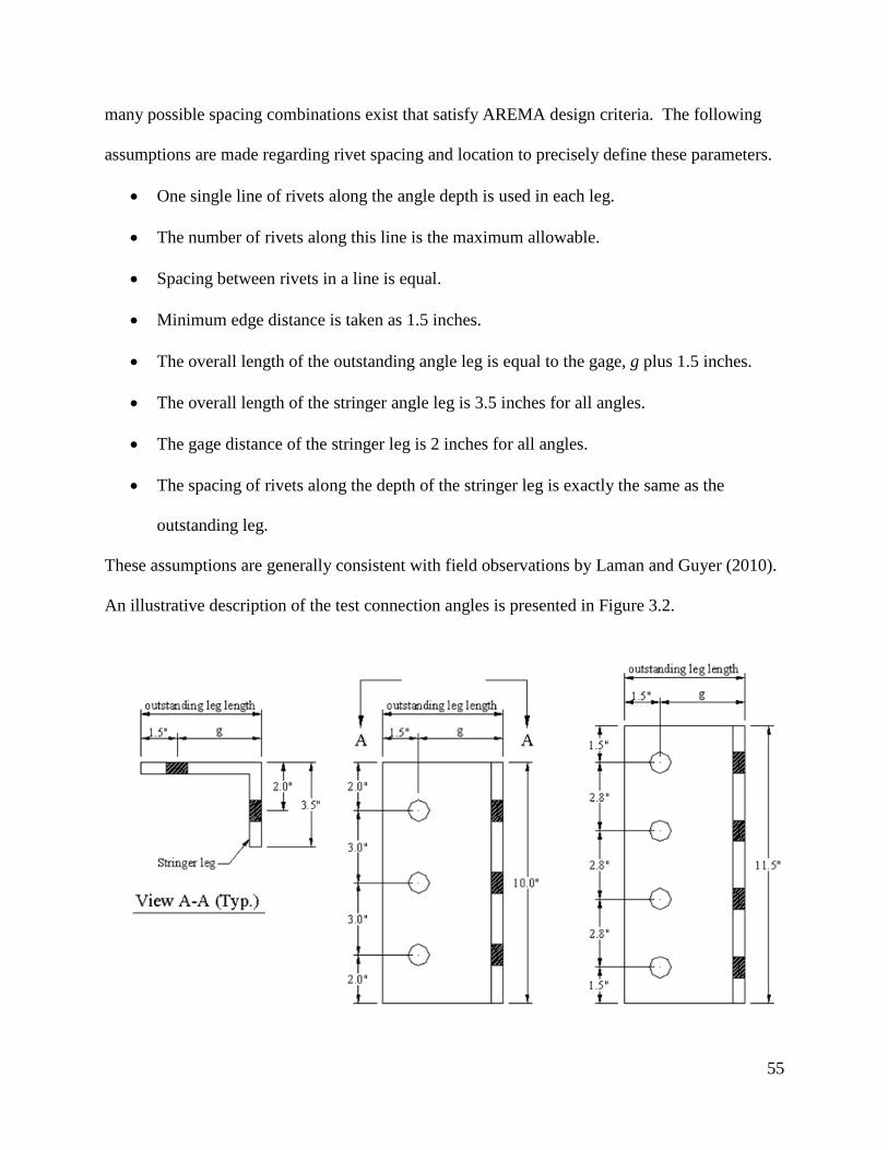
55
many possible spacing combinations exist that satisfy AREMA design criteria. The following
assumptions are made regarding rivet spacing and location to precisely define these parameters.
• One single line of rivets along the angle depth is used in each leg.
• The number of rivets along this line is the maximum allowable.
• Spacing between rivets in a line is equal.
• Minimum edge distance is taken as 1.5 inches.
• The overall length of the outstanding angle leg is equal to the gage, g plus 1.5 inches.
• The overall length of the stringer angle leg is 3.5 inches for all angles.
• The gage distance of the stringer leg is 2 inches for all angles.
• The spacing of rivets along the depth of the stringer leg is exactly the same as the
outstanding leg.
These assumptions are generally consistent with field observations by Laman and Guyer (2010).
An illustrative description of the test connection angles is presented in Figure 3.2.

56
Figure 3.2 Descriptions of Test Angles
3.2.2.2 Stringer Stiffness
Stringer design according to AREMA (2008a) is based on approximate analysis by assuming
the member is simply supported and thus statically determinate. Design load effects are easily
computed and a cross section is selected that satisfies both strength and serviceability criteria.
The purpose of this study is to consider rotational stiffness of stringer end connections, thus the
stringer beam is statically indeterminate. In order to analyze the statically indeterminate stringer,
specifically end moment, stringer stiffness must be defined.
Stringer stiffness is determined for this study according to AREMA (2008a) design
specifications and with the following assumptions:
• Cooper E-80 design load (defined in Figure 2.1);

57
• Design impact, IM = 55.8% (for 45mph speed);
• Live load is distributed equally to two stringers.
• Stringer acts non-compositely with track structure.
• Tensile bending stress in gross section controls design.
• Stringer cross section is symmetric.
• Allowable bending stress, Fb = 0.55Fy.
• Stringer length and stringer depth are defined in Table 3.1.
AREMA (2008a) provides tabulated maximum moment values, Mmax for Cooper E-80 design
load for various span lengths, including 8, 10, 12, and 14 feet. Required stringer stiffness in
terms of moment of intertia, Ireq’d is evaluated by the following equation:
ydreq F
pthstringerdeIMMI
55.0)2/()1(max
'×+×
= (3.2)
It is noted that the tabulated moment values in AREMA (2008a) are for one-half track loaded.
With the aforementioned assumption of equal load distribution to each stringer, this tabulated
moment is completely resisted by one stringer. Input values for equation 3.2 and calculated Ireq’d
are tabulated in Table 3.3.

58
Table 3.3 Required Stringer Moment of Inertia
3.2.3 Non-Variable Parameters
In addition to the independent and dependent parameters presented in previous sections,
several constant parameters values must be defined for this study. These parameters have been
set constant because they are either outside the scope of this study and/or do not vary
significantly. Non-variable parameters are:
(1) Rivet diameter
(2) Rivet clamping force
(3) Friction coefficient
(4) Material constants
(5) Fatigue Vehicle
Each of these are discussed and their constant values are define in the following sections.
Stringer Length, L
Angle Depth, d Stringer Depth M max (E-80) IM F b I req'd
feet inches inches k-ft ksi inches4
10 12.5 80 55.8% 19.8 47211.5 14.4 80 55.8% 19.8 54313 16.3 80 55.8% 19.8 61410 12.5 112.5 55.8% 19.8 664
11.5 14.4 112.5 55.8% 19.8 76413 16.3 112.5 55.8% 19.8 863
11.5 14.4 160 55.8% 19.8 108613 16.3 160 55.8% 19.8 1228
14.5 18.1 160 55.8% 19.8 136913 16.3 220 55.8% 19.8 1688
14.5 18.1 220 55.8% 19.8 188316 20.0 220 55.8% 19.8 2077
8
10
12
14

59
3.2.3.1 Rivet Diameter
Rivet shaft diameter of ⅞ inch and head diameter of 1⅜ inch is used for all rivets in this
study. Field measurements by Laman et al. (2001) and Laman and Guyer (2010) confirm these
values as typical. Additionally, AREMA (2008a) specifies that rivet diameter shall not exceed
one-quarter of the width of angle leg in which they are used. This criterion is satisfied for all
connections by using ⅞ inch rivet diameter.
3.2.3.2 Rivet Clamping Force
As discussed in Chapter 2, DePiero et al. (2002) defined rivet clamping force as 25 kips for
FE modeling. Based on engineering judgment, this value is suspected to be high so a lesser
value of 15 kips is used for all connections in this study. It is noted that the sensitivity of rivet
clamping force in a preliminary FE model was investigated. Clamping force of 25, 20 and 15
kips were applied in separate analyses. The difference in the effect of these clamping forces on
the moment-rotation behavior was not significant. Moreover, 15 kips is within the range of valid
rivet clamping force and variable rivet clamping force is outside the scope of this study.
3.2.3.3 Friction Coefficient
A review of previous FE modeling in Chapter 2 indicates that friction coefficients, µ range
from 0.3 to 0.5. Additionally, AISC (2005) specifies friction coefficient of 0.35 for unpainted
steel with mill scale and 0.5 for blast-cleaned steel surfaces. Based on AISC (2005) criteria, 0.35
is the ideal value to use based on surface condition. When correlating experimental laboratory
results to FE modeling results, sensitivity of μ was investigated by considering several different
values within the stated range. Variations in μ had little effect on FE results and μ defined as 0.5
provided slightly better correlation than other values. Based on this investigation, a friction
coefficient of 0.5 is used throughout this study.

60
3.2.3.4 Material Constants
All parts that make up the FE connection model assembly are modeled with elastic, perfectly
plastic steel. The modulus of elasticity, E and yield stress, Fy are equal to 29,000 ksi and 36 ksi
respectively. Poison’s ratio, ν is defined as 0.3.
3.2.3.5 Fatigue Vehicle
AREMA (2008a) does not specify a specific vehicle to use in fatigue analysis. Instead, the
fatigue vehicle is typically a specific equipment load that is operated on that railroad. The
literature review in Chapter 2 identified the 286,000 pound GCW, defined in Figure 2.2 as the
most common equipment load on current railroads. Also, research by Laman and Guyer (2010)
indicates that the 286,000 pound GCW equipment load is commonly used by Pennsylvania short-
line railroads to evaluate bridge load adequacy. The 286,000 pound GCW is used as the fatigue
vehicle in this study. Additionally impact load is also considered in fatigue analysis. For an
operating speed of 45 mph, AREMA (2008a) specifies a fatigue impact load of 20% for stringer.
3.3 Parametric Study Framework
The proposed numerical parametric study is performed with FE modeling using ABAQUS
6.9 and SAP2000 v14. Finite element programs are common analysis tools used by researchers
to evaluate various structural problems that otherwise would have to be performed in the field or
laboratory and would presumably require extensive resources. The following section presents a
stepwise procedure which outlines the framework for the parametric study.

61
3.3.1 Procedure
Step 1: Model Validation
Caution must be used when examining finite element analysis (FEA) results because an incorrect
model definition can render results invalid. When performing extensive FEA studies, it is
imperative to collect trusted comparative data that can be used to validate FEA results. Before
proceeding with this parametric study, FE model definitions and analysis procedures are
validated along with FEA results. Laboratory testing of two double angle connections provide
comparison data for corresponding FE models. Figure 3.3 shows the testing of one laboratory
specimen. Moment-rotation and stress results are compared between the laboratory and FE
models. Discrepancies in data are identified, addressed and model modifications are made as
necessary to predict experimental results. Detailed discussion of experimental laboratory testing
follows in Chapter 4.
Figure 3.3 Laboratory Testing of Double Angle Connection

62
Step 2: 3D FE Model of Double Angle Connection
A complete 3D FE model of an entire stringer with double angle end connections is a laborious
task to create in addition to the high computational demand for analysis. Recalling that 72
analysis cases are evaluated in this study, complete 3D FE modeling for each is not feasible. The
study is simplified by considering a localized 3D FE model of only the double angle connection
and a separate but corresponding 2D FE model which includes the stringer beam. The localized
3D connection model is defined by independent parameters: t, g and d. It can be observed from
Table 3.2 that there are only 37 unique combinations for these three parameters, thus only 37 3D
FE models are required to investigate all 72 cases. The 3D FE model is further simplified by
considering a longitudinal plane of symmetry such that only one connection angle is modeled as
shown in Figure 3.4. Detailed discussion of 3D FE modeling is presented in Chapter 5. Upon
completion of the 3D FEA, results are investigated.
Figure 3.4 Typical 3D FE Connection Model Assembly (ABAQUS)

63
Step 3: Develop Moment-Rotation Curve
In order to proceed with subsequent 2D FE modeling of the stringer beam, behavioral
characteristics of the connection must first be quantified. As discussed in Chapter 2, the most
important connection characteristic is the moment-rotation relationship. For each of the 37
connection models analyzed in step 2, a corresponding moment-rotation curve is developed from
3D FEA data. Recalling that only one connection angle is modeled as part of the 3D FEA and
that the present study is for double angle connections, an adjustment must be made to represent
modeling results in terms of the actual double angle connection. The adjustment is simply a
factor of 2 since one angle theoretically resists one-half the load. Thus, the magnitude of
moment represented on the moment-rotation curve is actually twice the applied moment from the
3D FEA. Figure 3.5 shows a typical moment-rotation curve for a double angle connection.
Figure 3.5 Typical Moment-Rotation Curve
0
5
10
15
20
25
30
35
0.000 0.002 0.004 0.006 0.008 0.010
Mom
ent,
M(k
-ft)
Rotation, θ (radians)
Moment-Rotation Curve
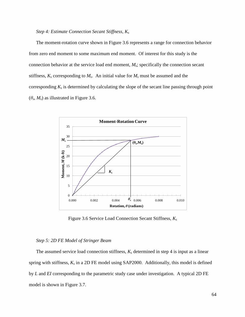
64
Step 4: Estimate Connection Secant Stiffness, Ks
The moment-rotation curve shown in Figure 3.6 represents a range for connection behavior
from zero end moment to some maximum end moment. Of interest for this study is the
connection behavior at the service load end moment, Ms; specifically the connection secant
stiffness, Ks corresponding to Ms. An initial value for Ms must be assumed and the
corresponding Ks is determined by calculating the slope of the secant line passing through point
(θs, Ms) as illustrated in Figure 3.6.
Figure 3.6 Service Load Connection Secant Stiffness, Ks
Step 5: 2D FE Model of Stringer Beam
The assumed service load connection stiffness, Ks determined in step 4 is input as a linear
spring with stiffness, Ks in a 2D FE model using SAP2000. Additionally, this model is defined
by L and EI corresponding to the parametric study case under investigation. A typical 2D FE
model is shown in Figure 3.7.
0
5
10
15
20
25
30
35
0.000 0.002 0.004 0.006 0.008 0.010
Mom
ent,
M(k
-ft)
Rotation, θ (radians)
Moment-Rotation Curve
Ks
Ms
θs
(θs,Ms)

65
Figure 3.7 Typical 2D FE Stringer Beam Model (SAP2000)
The 286,000 pound GCW moving fatigue vehicle load is applied to this 2D model and the
magnitude of the resulting end moment is compared to the assumed value, Ms from step 4. If the
values agree within 2% the study continues with step 7. If the values do not agree within 2%,
iteration must be performed until the values converge.
Step 6: Iterate
An iterative process must be performed to obtain convergence between the value of Ms, used
to estimate Ks and the resulting value of end moment from 2D FEA. The procedure returns to
step 4 using the 2D FEA end moment as the new initial Ms. A corresponding Ks is computed and
step 5 is repeated.
Step 7: Evaluate Connection Angle Stress
From steps 4 through 6, Ms is determined for a double connection configuration defined by
independent parameters, t, g, d, and L subject to the 286,000 pound GCW fatigue vehicle load.
The corresponding stress concentrations and magnitude are examined in the connection angles
by returning to the 3D FEA results. (As discussed in step 2, a scale factor of 2 must be used to
equate 3D FEA load to the actual connection load.) The principal stress magnitude

66
corresponding to Ms is effectively the cyclic stress range that occurs in the connection angle from
the passing of the fatigue vehicle.
3.4 Summary
This chapter presented the design of the parametric study. Parameters were identified and
discussed in detail to explain the applicability on the behavior of double angle connections.
Parameters were grouped as primary independent, dependant, and non-variable. Values for each
parameter were identified and justified based on previous studies and engineering judgment as it
relates scope of the present study. Seventy-two unique parametric study analysis cases were
presented along with the general procedure by which they are analyzed.

67
Chapter 4
EXPERIMENTAL DESIGN AND TESTING
4.1 Introduction
This chapter presents experimental laboratory testing of two double angle connection
specimens. The main objectives of the experimental program are to establish moment-rotation
behavior of the connection and measure stress at critical locations on the connection angle. The
purpose of the experimental testing was to provide a data set to be used in the calibration of
companion FE models. The experimental test design and test set-up is discussed in detail, as
well as test procedures and results.
4.2 Experimental Test Design and Specimens
Similar to experimental studies by Astaneh et al. (1989) and Hong et al. (2002) discussed in
Chapter 2, the current experimental study evaluated two cantilevered beam specimens connected
to a rigid support with a double angle connection. Figure 4.1 presents the test design and Figure
4.2 presents photos of a test specimen in the load frame.
The W12×26 cantilever beam is 26 inches long and was evaluated for bearing strength at bolt
holes in the web according to AISC (2005) Chapter J. The ¼ inch nominal web thickness is not
adequate to resist the experimental load, therefore a ¼ inch doubler plate was welded on both
sides of the web to increase the thickness of material in bearing to ¾ inch.
The WT16.5×65 was obtained by cutting a waste piece of W33×130 section in half along its
strong axis. The WT section, configured as shown in Figure 4.1, is an ideal mounting surface for
the double angle connection because it is sufficiently stiff to be approximated as a fixed surface.

68
Figure 4.1 Experimental Test Design

69
Figure 4.2 Experimental Test Specimen 1
The experimental study consisted of evaluating two test specimens. The specimens are
identical except for the outstanding leg gage distance of the angles. Gage distances of 2.25 and
3.75 inches are used for specimen 1 and 2 respectively. These distances represent a stiff and
flexible connection. The size of connection angles used for both specimens is L5×3×½ by 10
inches long. Each specimen was assembled with ¾ inch diameter ASTM A-307 bolts. Based on
Kulak et al. (2001), this bolt type was selected rather than A-325 and A-490 because it is a low
carbon steel material that is similar to rivet steel. Bolt holes were drilled to a diameter of 13/16
inches.
Load was applied from a hydraulic actuator through a 220 kip load cell. The head of the 220
kip load cell is fixed so once the specimen is centered in the load frame, sufficient friction
existed at the beam and load cell interface that lateral bracing was not required. The specimen
was configured so that the point of application of load was 24 inches from the face of the
WT16.5×65 flange. Consequently, the connection end moment is determined from the product
of 24 inches and the magnitude of applied force measured in the load cell.

70
4.3 Test Set-Up and Instrumentation
Before the test specimens were bolted together, each connection angle was instrumented with
bondable foil strain gages. Three uni-axial strain gages with a gage length of 0.250 inches were
installed on each connection angle for specimen 1 as shown in Figure 4.3 and pictured in Figure
4.4. These strain gages provide microstrain measurements in the direction parallel to the gage.
Figure 4.3 Detail of Strain Gage Placement on Test Specimen 1
Figure 4.4 Installed Strain Gages, Specimen 1

71
Strain gages could be placed anywhere on the angle as long as it is possible to make a stress
comparison with that same point on the FE model; however it is desirable to place strain gages at
areas of interest. A literature review of Chapter 2 identified the toe of the fillet on the
outstanding leg of the connection angle as an area of high stress. Thus stain gages were placed
as shown in Figure 4.3 and 4.4, near the toe of the fillet on the outstanding leg of specimen 1.
The gage placement on specimen 2 differs from specimen 1 in that a total of eight uni-axial
gages are placed on specimen 2 as shown in Figures 4.5 and 4.6. Specimen 2 gage locations
were selected to evaluate the toe of the fillet on the stringer leg in addition to the toe of fillet on
the outstanding leg.
Figure 4.5 Detail of Strain Gage Placement on Test Specimen 2
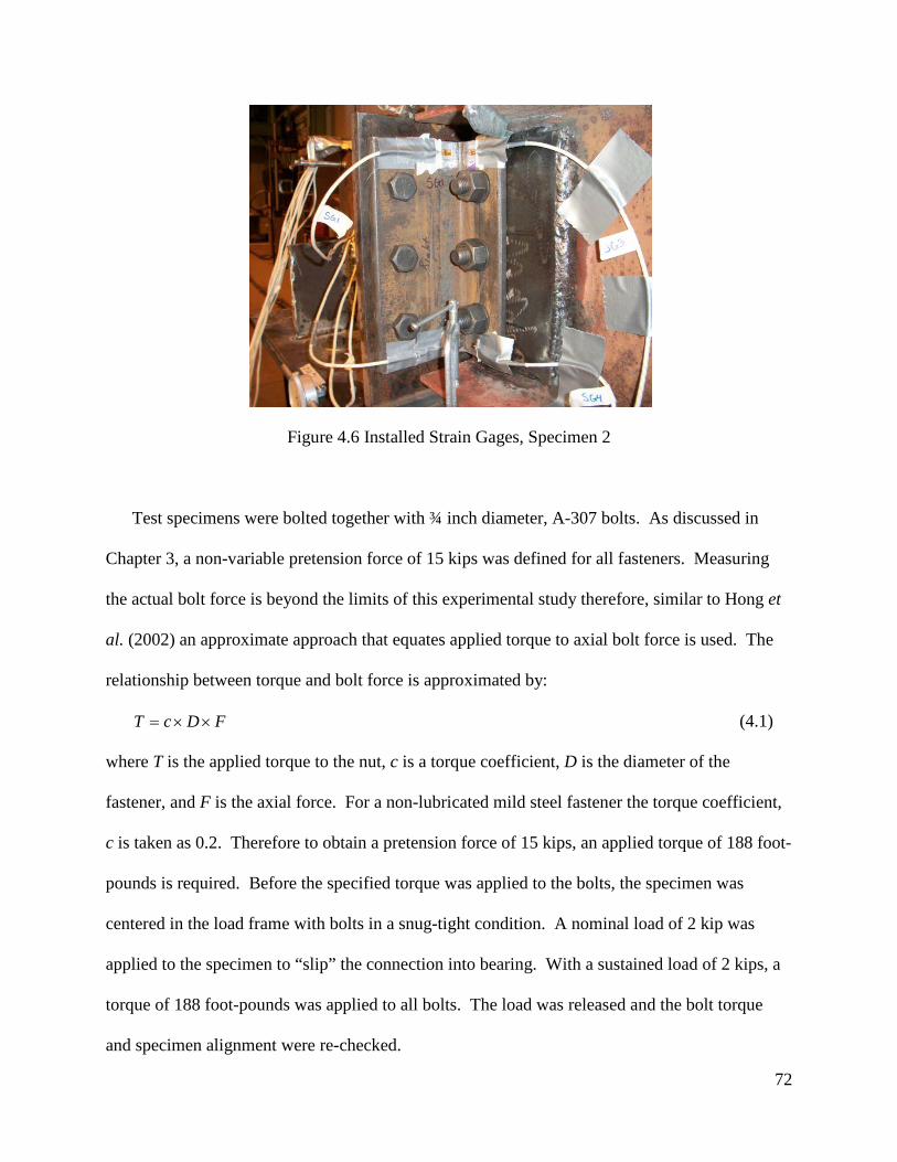
72
Figure 4.6 Installed Strain Gages, Specimen 2
Test specimens were bolted together with ¾ inch diameter, A-307 bolts. As discussed in
Chapter 3, a non-variable pretension force of 15 kips was defined for all fasteners. Measuring
the actual bolt force is beyond the limits of this experimental study therefore, similar to Hong et
al. (2002) an approximate approach that equates applied torque to axial bolt force is used. The
relationship between torque and bolt force is approximated by:
FDcT ××= (4.1)
where T is the applied torque to the nut, c is a torque coefficient, D is the diameter of the
fastener, and F is the axial force. For a non-lubricated mild steel fastener the torque coefficient,
c is taken as 0.2. Therefore to obtain a pretension force of 15 kips, an applied torque of 188 foot-
pounds is required. Before the specified torque was applied to the bolts, the specimen was
centered in the load frame with bolts in a snug-tight condition. A nominal load of 2 kip was
applied to the specimen to “slip” the connection into bearing. With a sustained load of 2 kips, a
torque of 188 foot-pounds was applied to all bolts. The load was released and the bolt torque
and specimen alignment were re-checked.

73
Rotation of the double angle connection was measured indirectly using dial gages in a similar
way that Astaneh et al. (1989) and Hong et al. (2002) used LVDT’s to measure displacement and
calculate rotation. The detailed typical placement of 3 dial gages (DG) is shown in Figure 4.7
and pictured in Figure 4.8.
Figure 4.7 Angle Rotation Measurement -- Detail of Dial Gage Placement

74
Figure 4.8 Angle Rotation Measurement -- Dial Gage Placement Photo
4.4 Test Procedure
The testing procedure is listed below:
• Begin with no load applied to specimen.
• Acquire and verify strain gage signal through data acquisition system.
• Set strain gage scan frequency to 1 Hz.
• Balance all strain gage channels.
• Record initial dial gage readings.
• Position load cell to initiate contact with specimen.
• Zero load cell force.
• Define constant load rate of 0.015in/min.
• Start test
• Record dial gage readings at every 0.5 kip increment.
• Stop test when rotation of 0.02 radians is reached or when deemed necessary.

75
. A constant displacement rate 0.015 inches per minute was used as opposed to manual start-
and-stop to prevent load leak-down in the actuator when paused. Displacement controlled
testing produces a continuous stream of strain and load data without discontinuities. However,
recording three dial gage readings simultaneously at 0.5 kip intervals under a continuous load
can prove challenging. To facilitate dial gage readings, the load rate of 0.015 inches per minute
was chosen. This rate was slow enough that three successive dial gage readings could be
considered instantaneous.
4.5 Experimental Test Results
4.5.1 Specimen 1 Results
Figure 4.9 presents the resulting moment-rotation curve from the experimental testing of
specimen 1.
Figure 4.9 Lab Specimen 1: Moment-Rotation Curve
0
5
10
15
20
25
0.000 0.005 0.010 0.015 0.020
Mom
ent (
k-ft
)
Rotation (radians)
Lab Specimen 1: Moment-Rotation Curve

76
Figure 4.10 presents the stain (stress) and applied moment relationship for lab specimen 1.
Figure 4.10 Lab Specimen 1: Filtered Strain (stress) vs Moment
The data points in Figure 4.10 were obtained by filtering out electronic noise from the raw data.
The filtering was performed using a moving average technique. It is noted that specimen 1 was
instrumented with six strain gages, three on each angle but only strain gages 1, 2, and 3 are
presented in Figure 4.10. A review of stain data from gages 4, 5 and 6 showed inconsistent data
and was deemed unreliable and not used as part of this study. Additionally, it was observed from
Figure 4.10 that in the moment range from 0 to 5 kip-feet, near zero strain was recorded for all
three gages. In the moment range from 5 to 10 kip-feet, near zero strain was recorded for strain
-21.75
-14.5
-7.25
0
7.25
14.5
21.75
29
-750
-500
-250
0
250
500
750
1000
0 5 10 15 20 25
Mic
rost
rain
Applied Moment (k-ft)
Lab Specimen 1: Filtered Strain (stress) vs Moment
SG1SG2SG3
Stre
ss (k
si)

77
gages 1 and 2. This anomaly in the recorded strain data is likely explained in part by the slipping
and misalignment of the connection surfaces. It was also observed that the mounting flange of
the WT16.5×65, pictured in Figure 4.11 is not a perfectly flat surface. Using a straight edge and
feeler gage, maximum warp across the flange surface was measured in excess of 0.030 inches.
Figure 4.11 Specimen Mounting Surface
The significance of flange warp is that as the specimen is loaded, the entire connection must
rotate and contort such that the compression area of the connection is able to bear on the
mounting flange. It was observed from the strain data in Figure 4.10 that full connection bearing
was not established until approximately 10 kip-feet of moment was applied. A post test
investigation also revealed misalignment between several bolt holes in the specimen. It was
observed that the top bolt hole in the stringer leg of the angles was misaligned by approximately
⅛ inche as pictured in Figure 4.12. This misalignment results in the bolt engaging one angle
before the other. Additional care was taken in the preparation of specimen 2 to mitigate these
issues.

78
Figure 4.12 Bolt Hole Misalignment in Specimen 1
4.5.2 Specimen 2 Results
Figure 4.13 and 4.14 present the resulting moment-rotation curve and strain verses applied
moment respectively from the experimental testing of specimen 2.
Figure 4.13 Lab Specimen 2: Moment-Rotation Curve
0
5
10
15
20
25
0 0.005 0.01 0.015 0.02
Mom
ent (
k-ft
)
Rotation (radians)
Lab Specimen 2: Moment-Rotation Curve

79
Figure 4.14 Lab Specimen 2: Averaged, Filtered Strain (stress) vs Moment
Similar to specimen 1, data points in Figure 4.14 were obtained by averaging raw data.
Additionally, all eight strain gages, four on each angle provided usable test data and symmetric
strain gages (1 and 5, 2 and 6, 3 and 7, 4 and 8) were averaged.
From a qualitative perspective, specimen 2 data is reasonable. Observations from the
moment-rotation curve in Figure 4.13 show a steeper initial slope followed by gradual bending
over. This is typical non-linear behavior of double angle connections. Also, as compared to the
moment-rotation curve for specimen 1 in Figure 4.9, specimen 2 exhibits less stiffness which is
expected for the increased gage of specimen 2. Strain data in Figure 4.14 shows expected
-29
-21.75
-14.5
-7.25
0
7.25
14.5
21.75
29
36.25
43.5
-1000
-750
-500
-250
0
250
500
750
1000
1250
1500
0 2 4 6 8 10 12
Mic
rost
rain
Applied Moment (k-ft)
Lab Specimen 2: Averaged, Filtered Strain (stress) vs Moment
SG1&5SG2&6SG3&7SG4&8
Stre
ss (k
si)
80
general trends. The highest tensile strain was expected in SG3 and 7 and lowest compressive
strain was expected in SG4 and 8.
4.6 Summary
This chapter discussed the design and testing of two double angle connection laboratory
specimens. The configuration for each specimen was identical except the gage distance of the
outstanding leg was 2.25 and 3.75 inches for specimen 1 and 2 respectively. The main objective
of the laboratory testing was to obtain moment-rotation and stress data that can be used in the
calibration and verification of companion FE models. The results of the testing from specimen 1
suggest that fabrication imperfections along with connection slip are the cause of irregularities in
data. Based on post test observations from specimen 1, specimen 2 was fabricated with
increased precision to minimize the source of errors. Additionally specimen 2 was subjected to a
series of low magnitude “shakedown” loads to slip the connection into bearing prior to the start
of the actual test. A qualitative assessment of data from the test of specimen 2 indicates that this
data is more reliable than data from specimen 1. A comparison of this test data with FEA results
is discussed in Chapter 5.

81
Chapter 5
NUMERICAL MODELING
5.1 Introduction
Numerical modeling techniques employed by this parametric study are presented in this
chapter. Finite element modeling techniques for double angle connections were investigated in
previous research by DePiero et al. (2002), Imam et al. (2007), Al-Emrani and Kliger (2002) and
Hong et al. (2002) and were used as a general guide in the development of FE models for the
present study. This study consists of both 2D and 3D FE models. ABAQUS version 6.9 was
used as the 3D numerical program to model a series of double angle connections. Experimental
laboratory testing results from two double angle connection specimens were used to calibrate and
validate preliminary 3D FE models. This validation process provided a level of confidence in
subsequent 3D FEA results used in the parametric study. SAP2000 version 14 was used as the
2D numerical program for the series of stringer beam models in the parametric study.
As discussed in Chapter 3, primary independent parameters considered in this parametric
study are gage distance, angle thickness, angle depth, and stringer length resulting in 72 analysis
cases. Because stringer length was not considered in the 3D FE connection model, only 37
unique 3D models are required. Connection stiffness obtained from 3D FEA moment-rotation
results was used to quantify connection behavior as a linear spring in 72 unique 2D stringer beam
models. Through an iterative process, the magnitude of connection end moment from the
286,000 pound GCW fatigue vehicle was determined from 2D FEA results. Maximum principal
stress in the angle was determined from the 3D model by considering the state of stress at the
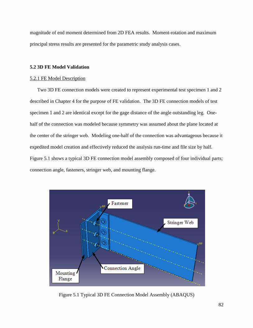
82
magnitude of end moment determined from 2D FEA results. Moment-rotation and maximum
principal stress results are presented for the parametric study analysis cases.
5.2 3D FE Model Validation
5.2.1 FE Model Description
Two 3D FE connection models were created to represent experimental test specimen 1 and 2
described in Chapter 4 for the purpose of FE validation. The 3D FE connection models of test
specimen 1 and 2 are identical except for the gage distance of the angle outstanding leg. One-
half of the connection was modeled because symmetry was assumed about the plane located at
the center of the stringer web. Modeling one-half of the connection was advantageous because it
expedited model creation and effectively reduced the analysis run-time and file size by half.
Figure 5.1 shows a typical 3D FE connection model assembly composed of four individual parts;
connection angle, fasteners, stringer web, and mounting flange.
Figure 5.1 Typical 3D FE Connection Model Assembly (ABAQUS)
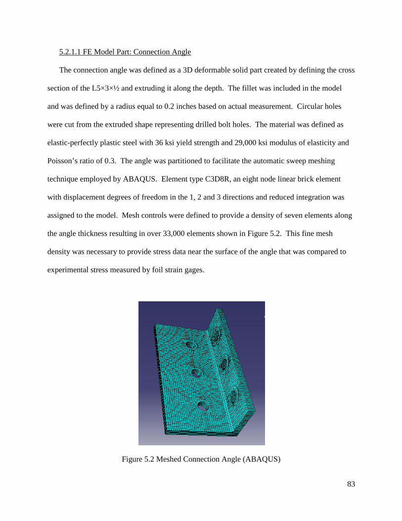
83
5.2.1.1 FE Model Part: Connection Angle
The connection angle was defined as a 3D deformable solid part created by defining the cross
section of the L5×3×½ and extruding it along the depth. The fillet was included in the model
and was defined by a radius equal to 0.2 inches based on actual measurement. Circular holes
were cut from the extruded shape representing drilled bolt holes. The material was defined as
elastic-perfectly plastic steel with 36 ksi yield strength and 29,000 ksi modulus of elasticity and
Poisson’s ratio of 0.3. The angle was partitioned to facilitate the automatic sweep meshing
technique employed by ABAQUS. Element type C3D8R, an eight node linear brick element
with displacement degrees of freedom in the 1, 2 and 3 directions and reduced integration was
assigned to the model. Mesh controls were defined to provide a density of seven elements along
the angle thickness resulting in over 33,000 elements shown in Figure 5.2. This fine mesh
density was necessary to provide stress data near the surface of the angle that was compared to
experimental stress measured by foil strain gages.
Figure 5.2 Meshed Connection Angle (ABAQUS)

84
5.2.1.2 FE Model Part: Fastener
The fastener is a 3D deformable solid part modeled to represent a ¾ inch diameter A-307
bolt used in the experimental specimens. Similar to modeling by Hong et al. (2002), a round
fastener head with diameter of 1.1 inches was used to idealize the actual hex head of the bolt.
Material was defined as steel with yield strength of 60 ksi [Kulak et al. 2001] and modulus of
elasticity and Poisson’s ratio of 29,000 ksi and 0.3 respectively. The entire cylindrical shank was
partitioned from the fastener head to facilitate meshing. Two element types were used to mesh
the fastener; C3D6 for the shank and C3D8R for the outer head as shown in Figure 5.3.
Figure 5.3 Meshed Fastener (ABAQUS)
Element type C3D6 is a six node linear triangular prism element that provided a more uniform
mesh for a circular section than a hexahedral element. The previously discussed C3D8R element
was used for the partitioned annulus fastener head. Mesh density was established by default
mesh seed sizing controls.

85
5.2.1.3 FE Model Part: Stringer Web
The primary purpose of the stringer web in the connection model shown in Figure 5.1 was to
transfer load into the connection angle. Rather than modeling the entire stringer shape with
deformable finite elements, only the stringer web was considered and was defined as a rigid
body. A rigid body is a collection of nodes and elements whose motion is governed by the
motion of a single node, called the rigid body reference node. The relative positions of the nodes
and elements that are part of the rigid body remain constant throughout a simulation. Therefore,
the constituent elements do not deform but can undergo large rigid body motions. The principal
advantage to representing portions of a model with rigid bodies rather than deformable finite
elements is computational efficiency because element-level calculations are not performed for
elements that are part of a rigid body [ABAQUS 2009]. As shown in Figure 5.4, three integral ¾
inch diameter studs were included in the model of the web. These studs represent the bolt shanks
that transfer load to the angle. It was realistic to model these as a rigid body because the actual
bolt shear deformations are very small relative to the connection angle bending deformations.
Figure 5.4 Rigid Body Stringer Web (ABAQUS)

86
5.2.1.4 FE Model Part: Mounting Flange
The mounting flange, like the stringer web, was modeled as a rigid body. The actual
mounting flange is very stiff relative to the connection and was therefore assumed non-
deformable. The primary function of the mounting flange in the model was to provide a
boundary surface for the deformable connection angle and fasteners. Figure 5.5 shows the rigid
body mounting flange.
Figure 5.5 Rigid Body Mounting Flange (ABAQUS)
5.2.1.5 Boundary Conditions
Boundary conditions were defined to place restrictions on available degrees of freedom, U1,
U2, and U3 within the model. Referring to Figure 5.1 and directions 1, 2 and 3 corresponding to
X, Y, and Z respectively, a boundary condition U3=0 was assigned to the stringer web. This
restricted translation of the rigid body to the X-Y plane. The mounting flange is fixed in space,
therefore boundary conditions of U1=U2=U3=0 were defined for this rigid body part, restricting
all translation. These boundary conditions were created in the initial step and propagated to all

87
subsequent analysis steps. Temporary boundary conditions were also created in the initial step to
“hold” parts in place until contact was established between defined contact surfaces. Temporary
boundary conditions include U1=U2=U3=0 applied to all three fasteners in the outstanding angle
leg and U1=U2=0 applied to stringer web. These boundary conditions were removed in the first
analysis step when contact was established.
5.2.1.6 Contact Interaction
The individual parts modeled by the assembly in Figure 5.1 were positioned so surfaces of
mating parts are in contact. ABAQUS numerical formulation does not recognize mating contact
surfaces according to their proximity. Therefore, to prevent one model surface from penetrating
another, contact interaction must be explicitly defined for all potential contact surfaces. Using
the ABAQUS command “find contact pairs”, all potential contact surfaces are identified.
General contact, surface-to-surface formulation was used to define contact between mating parts.
Contact interaction was defined by both normal and tangential contact properties. Normal
contact property was defined as “hard contact” that allows surface separation after contact.
Tangential contact property was defined as friction “penalty” with a coefficient of friction
defined as 0.5. Contact was initiated in analysis step 1 with a very small initial time increment
defined as 0.01. The size of subsequent time increments was automatically adjusted based on
how quickly the solution converges. After contact was established, load was applied to the
model.
5.2.1.7 Applied Load
An equivalent clamping force was applied at all fasteners to simulate in-situ force of 15 kips.
Clamping force was induced in each of the three fasteners in the outstanding leg with a specified
equivalent displacement according to Hooke’s Law. The displacement, in the negative U1

88
direction was applied to the face of the bolt shank. An effective clamping force was also applied
at the three stringer web studs with a specified equivalent pressure load on the surface of the
angle, acting over a representative bearing area of the fastener head. Web clamping force was
applied in analysis step 2 and held constant throughout subsequent analysis steps.
Beginning with analysis step 3, load was applied to the model simulating live load.
Incremental load was applied with a series of sequential events defined by general nonlinear
analysis steps. That is the state of the model at the end of one general step provides the initial
state for the start of the next general step. Each analysis step represents a moment of 0.5 kip-
feet, consistent with the interval that dial gage readings were recorded in the experimental study.
5.2.2 Comparison with Experimental Results
Moment-rotation and stress between experimental and numerical evaluations for double
angle connection specimens 1 and 2 are compared as well as visual observations of deformation
behavior. Figure 5.6 and 5.7 present moment-rotation and stress comparisons respectively for
specimen 1. Comparison of moment-rotation and stress for specimen 2 is presented in Figure 5.8
and 5.9. Qualitative visual comparison of connection deformation behavior for specimen 2 is
presented in Figure 5.10.

89
Figure 5.6 Specimen 1: Moment-Rotation of Experimental and Numerical
Figure 5.7 Specimen 1: Experimental vs Numerical - All Gage Locations
0
5
10
15
20
25
0.000 0.005 0.010 0.015 0.020
Mom
ent (
k-ft
)
Rotation (radians)
Specimen 1: Moment-Rotation Comparison
Exp.Num.
-21.75
-14.5
-7.25
0
7.25
14.5
21.75
29
-750
-500
-250
0
250
500
750
1000
0 5 10 15 20 25
Mic
rost
rain
Applied Moment (k-ft)
Specimen 1: Strain (stress) vs Moment Comparison
Exp. SG1Exp. SG2Exp. SG3Num. SG1Num. SG2Num. SG3St
ress
(ksi
)

90
Figure 5.8 Specimen 2: Moment-Rotation of Experimental and Numerical
Figure 5.9 Specimen 2: Experimental vs Numerical – All Gage Locations
0
5
10
15
20
25
0 0.005 0.01 0.015 0.02
Mom
ent (
k-ft
)
Rotation (radians)
Specimen 2: Moment-Rotation Comparison
Exp.Num.
-29
-21.75
-14.5
-7.25
0
7.25
14.5
21.75
29
36.25
43.5
-1000
-750
-500
-250
0
250
500
750
1000
1250
1500
0 2 4 6 8 10 12
Mic
rost
rain
Applied Moment (k-ft)
Specimen 2: Strain (stress) vs Moment Comparison
Exp. SG1,5Exp. SG2,6Exp. SG3,7Exp. SG4,8Num. SG1,5Num. SG2,6Num. SG3,7Num. SG4,8
Stre
ss (k
si)

91
a) Experiment Deformation, View from
Above
b) Numerical Model Deformation, View
from Above
Figure 5.10 Specimen 2: Deformed Shape Comparison – Experimental and Numerical
5.2.3 Discussion
Comparison of moment-rotation for specimen 1and 2 presented in Figure 5.6 and 5.8
respectively shows the initial slope of numerical modeling results steeper than experimental
results. Recalling from Chapter 3 that Ks is quantified by the slope of a line secant to the curve
that passes through the origin; numerical results indicate a stiffer connection. Percent difference
between numerical and experimental stiffness for specimen 1 and 2 is quantified in Table 5.1.
Significant difference between numerical and experimental Ks is observed in Table 5.1.
However, it is reasoned that numerical results are satisfactory to proceed with the parametric
study of riveted double angle connections. The following discussion provides the justification
for the decision to proceed.

92
Table 5.1 Experimental Connection Stiffness Comparison
Initially discussed in Chapter 4, experimental results for specimen 1 include effects from
connection slip and fabrication imperfections; both decrease connection stiffness. A qualitative
review of experimental data in Figure 5.6 indicates the connection was fully engaged between 8
and 9 kip-feet followed by slip that occurred between 9 and 10 kip-feet. From 10 to 12 kip-feet
the connection showed full bearing behavior. This behavior is evident by observing the sharp
slope changes in the moment-rotation curve. A sharp increase indicates full bearing and a sharp
decrease indicates slip. A visual comparison of the experimental and numerical slopes between
8 and 9, and 10 and 12 kip-feet shows much better agreement than the overall curve. This
Specimen 1 Specimen 2Stiffness, K s Stiffness, K s
(k-ft) (% Difference) (% Difference)1 55% 30%2 69% 1%3 74% 17%4 75% 26%5 77% 33%6 78% 42%7 79% 49%8 80% 54%9 78% 56%
10 78% 59%11 77% 61%12 77% 61%13 78% 59%14 79% 57%15 79% 52%16 80% -17 79% -18 77% -19 74% -20 70% -
Moment
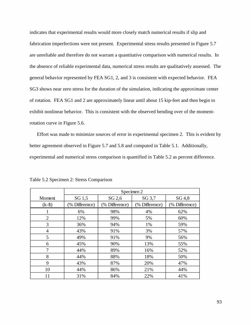
93
indicates that experimental results would more closely match numerical results if slip and
fabrication imperfections were not present. Experimental stress results presented in Figure 5.7
are unreliable and therefore do not warrant a quantitative comparison with numerical results. In
the absence of reliable experimental data, numerical stress results are qualitatively assessed. The
general behavior represented by FEA SG1, 2, and 3 is consistent with expected behavior. FEA
SG3 shows near zero stress for the duration of the simulation, indicating the approximate center
of rotation. FEA SG1 and 2 are approximately linear until about 15 kip-feet and then begin to
exhibit nonlinear behavior. This is consistent with the observed bending over of the moment-
rotation curve in Figure 5.6.
Effort was made to minimize sources of error in experimental specimen 2. This is evident by
better agreement observed in Figure 5.7 and 5.8 and computed in Table 5.1. Additionally,
experimental and numerical stress comparison is quantified in Table 5.2 as percent difference.
Table 5.2 Specimen 2: Stress Comparison
Moment SG 1,5 SG 2,6 SG 3,7 SG 4,8(k-ft) (% Difference) (% Difference) (% Difference) (% Difference)
1 6% 98% 4% 62%2 12% 99% 5% 60%3 36% 94% 1% 59%4 43% 91% 3% 57%5 49% 91% 9% 56%6 45% 90% 13% 55%7 44% 89% 16% 52%8 44% 88% 18% 50%9 43% 87% 20% 47%10 44% 86% 21% 44%11 31% 84% 22% 41%
Specimen 2
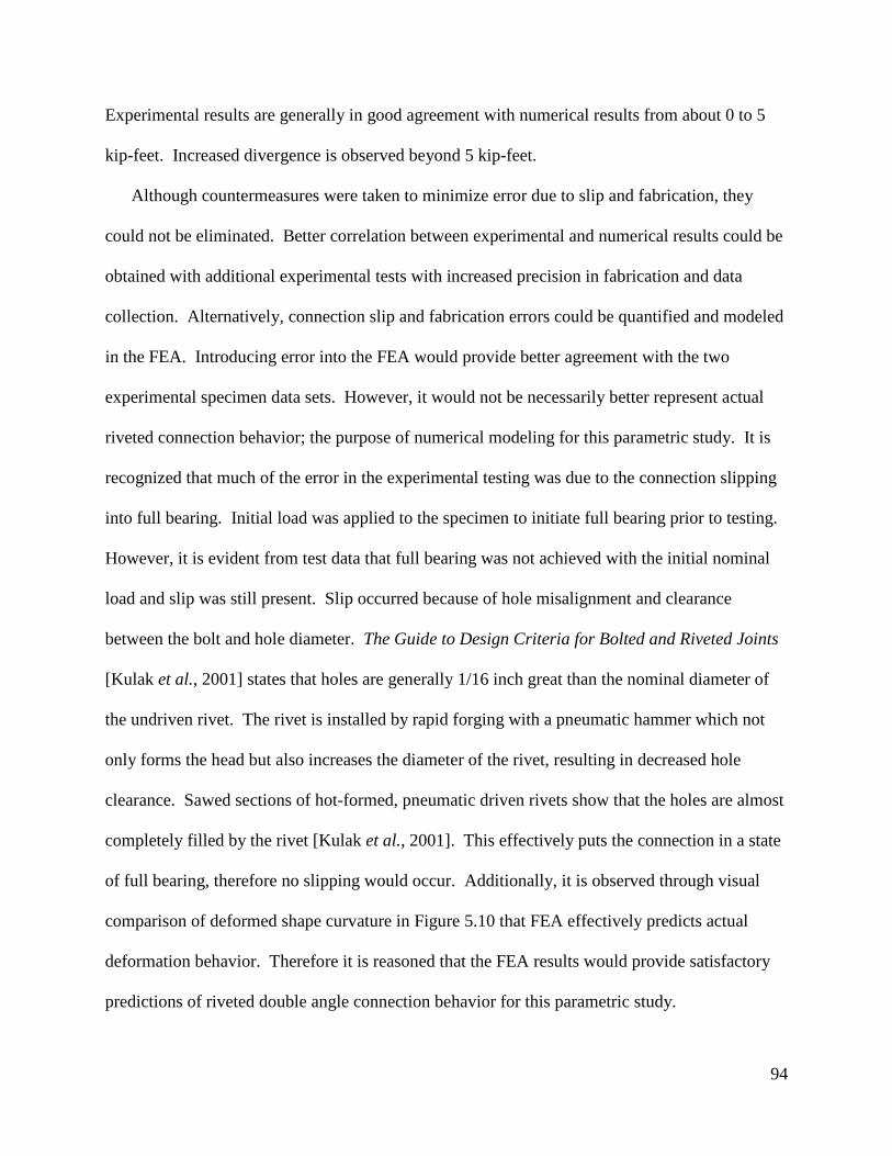
94
Experimental results are generally in good agreement with numerical results from about 0 to 5
kip-feet. Increased divergence is observed beyond 5 kip-feet.
Although countermeasures were taken to minimize error due to slip and fabrication, they
could not be eliminated. Better correlation between experimental and numerical results could be
obtained with additional experimental tests with increased precision in fabrication and data
collection. Alternatively, connection slip and fabrication errors could be quantified and modeled
in the FEA. Introducing error into the FEA would provide better agreement with the two
experimental specimen data sets. However, it would not be necessarily better represent actual
riveted connection behavior; the purpose of numerical modeling for this parametric study. It is
recognized that much of the error in the experimental testing was due to the connection slipping
into full bearing. Initial load was applied to the specimen to initiate full bearing prior to testing.
However, it is evident from test data that full bearing was not achieved with the initial nominal
load and slip was still present. Slip occurred because of hole misalignment and clearance
between the bolt and hole diameter. The Guide to Design Criteria for Bolted and Riveted Joints
[Kulak et al., 2001] states that holes are generally 1/16 inch great than the nominal diameter of
the undriven rivet. The rivet is installed by rapid forging with a pneumatic hammer which not
only forms the head but also increases the diameter of the rivet, resulting in decreased hole
clearance. Sawed sections of hot-formed, pneumatic driven rivets show that the holes are almost
completely filled by the rivet [Kulak et al., 2001]. This effectively puts the connection in a state
of full bearing, therefore no slipping would occur. Additionally, it is observed through visual
comparison of deformed shape curvature in Figure 5.10 that FEA effectively predicts actual
deformation behavior. Therefore it is reasoned that the FEA results would provide satisfactory
predictions of riveted double angle connection behavior for this parametric study.

95
5.3 Parametric Study 3D FE Modeling
The general 3D FE model description presented in the previous section was used to for the
parametric study double angle connection analysis cases. Fastener and hole diameters were
increased to ⅞ inch and the mounting plate and stringer web parts were modified as necessary to
connect to each of the 37 connection angles defined in Chapter 3. Additionally, mesh density of
the connection angle was also modified for the parametric study.
Mesh density for the verification angle included over 33,000 elements, requiring
considerable computational effort that resulted in long analysis run time. In an effort to decrease
analysis time while preserving accuracy of FEA, mesh sensitivity was investigated. Mesh
densities with nominal element sizes of ¼ and ⅛ inch were modeled and FEA results were
compared with the origin mesh. Moment-rotation was very similar with both meshes, however
stress results were much less accurate with the ¼ inch mesh due to the larger element volume.
The FEA results with the ⅛ inch connection angle mesh provided good agreement with the
original model and consisted of approximately 40% fewer elements. This considerably reduced
the analysis run time and did not have a significant effect on FEA results. Based on this
evaluation, all parametric study connection angles were meshed with ⅛ inch nominal element
size.
5.4 Parametric Study 2D FE Modeling
2D modeling of statically indeterminate stringer beams was performed using SAP2000. The
model, consisting of a single frame object representing the stringer beam is shown in Figure 5.11
along with axis orientation. Steel material properties were defined as well as the moment of
inertia for the analysis case. The frame object is a single beam element with displacement
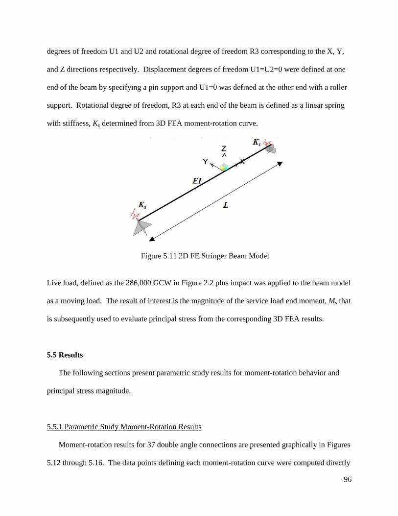
96
degrees of freedom U1 and U2 and rotational degree of freedom R3 corresponding to the X, Y,
and Z directions respectively. Displacement degrees of freedom U1=U2=0 were defined at one
end of the beam by specifying a pin support and U1=0 was defined at the other end with a roller
support. Rotational degree of freedom, R3 at each end of the beam is defined as a linear spring
with stiffness, Ks determined from 3D FEA moment-rotation curve.
Figure 5.11 2D FE Stringer Beam Model
Live load, defined as the 286,000 GCW in Figure 2.2 plus impact was applied to the beam model
as a moving load. The result of interest is the magnitude of the service load end moment, Ms that
is subsequently used to evaluate principal stress from the corresponding 3D FEA results.
5.5 Results
The following sections present parametric study results for moment-rotation behavior and
principal stress magnitude.
5.5.1 Parametric Study Moment-Rotation Results
Moment-rotation results for 37 double angle connections are presented graphically in Figures
5.12 through 5.16. The data points defining each moment-rotation curve were computed directly

97
from FEA displacement output at each analysis step; analogous to dial gage readings in the
experimental study. These connections are uniquely defined by the parameters: d, t, and g.
Results are grouped such that for a given d the effect of t and g can quickly and easily be
observed. Moment range and resulting rotations in Figures 5.12 through 5.16 were established to
capture the 286,000 pound GCW service level load effect. Connection behavior at load levels
significantly above the 286,000 pound GCW are beyond the scope of this study.
General trends in moment-rotation curves observed from Figures 5.12 through 5.16 are:
• Slope (Stiffness, Ks) increases with d
• Slope (Stiffness, Ks) increases with t
• Slope (Stiffness, Ks) increases with decreasing g
• Curves are non-linear but not to a high degree
Figure 5.12 Numerical Moment-Rotation Curves for d=10”
0
5
10
15
20
25
30
35
40
45
50
0.000 0.001 0.002 0.003 0.004
Mom
ent (
k-ft
)
Rotation (radians)
Moment-Rotation Curves for d=10"
t=0.5", g=2.0"t=0.5", g=2.5"t=0.5", g=3.0"t=0.625", g=2.0"t=0.625", g=2.5"t=0.625", g=3.0"

98
Figure 5.13 Numerical Moment-Rotation Curves for d=11.5”
Figure 5.14 Numerical Moment-Rotation Curves for d=13”
0
5
10
15
20
25
30
35
40
45
50
0.000 0.001 0.002 0.003 0.004
Mom
ent (
k-ft
)
Rotation (radians)
Moment-Rotation Curves for d=11.5"
t=0.5", g=2.0"t=0.5", g=2.5"t=0.5", g=3.0"t=0.5", g=3.5"t=0.625", g=2.0"t=0.625", g=2.5"t=0.625", g=3.0"t=0.625", g=3.5"
0
5
10
15
20
25
30
35
40
45
50
0.000 0.001 0.002 0.003 0.004
Mom
ent (
k-ft
)
Rotation (radians)
Moment-Rotation Curves for d=13"
t=0.5", g=2.0"t=0.5", g=2.5"t=0.5", g=3.0"t=0.5", g=3.5"t=0.625", g=2.0"t=0.625", g=2.5"t=0.625", g=3.0"t=0.625", g=3.5"t=0.625", g=4.0"

99
Figure 5.15 Numerical Moment-Rotation Curves for d=14.5”
Figure 5.16 Numerical Moment-Rotation Curves for d=16”
0
5
10
15
20
25
30
35
40
45
50
0.000 0.001 0.002 0.003 0.004
Mom
ent (
k-ft
)
Rotation (radians)
Moment-Rotation Curves for d=14.5"
t=0.5", g=2.5"t=0.5", g=3.0"t=0.5", g=3.5"t=0.625", g=2.5"t=0.625", g=3.0"t=0.625", g=3.5"t=0.625", g=4.0"
0
5
10
15
20
25
30
35
40
45
50
0.000 0.001 0.002 0.003 0.004
Mom
ent (
k-ft
)
Rotation (radians)
Moment-Rotation Curves for d=16"
t=0.5", g=2.5"t=0.5", g=3.0"t=0.5", g=3.5"t=0.625", g=3.0"t=0.625", g=3.5"t=0.625", g=4.0"

100
5.5.2 Parametric Study Principal Stress Results
The magnitude of maximum principal connection angle stress was evaluated by considering
the state of stress at service level moment, Ms as determined from 2D FEA. Figure 5.17, 5.18
and 5.19 show typical maximum principal stress distribution in the connection angle. It is
observed that high stress is concentrated near the fillet area over the top half of the angle. More
specifically, the maximum magnitude of principal stress in all 72 analysis cases occurred at the
fillet toe on the stringer leg of the angle, even with the top fasteners. This location is identified
in Figure 5.18 (b). Maximum principal stress, σp_max and corresponding service end moment, Ms
are presented in Table A-1 for each analysis case. Additionally, Ks corresponding to Ms is listed
for each case. General trends observed in Table A-1 when all other parameters are held constant
are:
• Service level connection moment, Ms increases with t
• Service level connection moment, Ms increases with L
• Service level connection moment, Ms increases with decreasing g
• Service level connection moment, Ms increases with d
• Maximum Principal Stress, σp_max increases with decreased t
• Maximum Principal Stress, σp_max increases with L
• Maximum Principal Stress, σp_max increases with decreasing g
• Maximum Principal Stress, σp_max does not vary significantly with change in d

101
Figure 5.17 Typical Numerical Model – General View- Maximum Principal Stress (ABAQUS)
a) Top View b) Section Cut at Top Fasteners
Figure 5.18 Typical Numerical Maximum Principal Stress Distribution: Plan View
Highest Stress Concentration
102
Figure 5.19 Typical Numerical Model – Maximum Principal Stress Distribution (ABAQUS)
5.6 Summary
Numerical modeling techniques employed in this parametric study have been presented in
detail. Two experimentally tested double angle connection specimens were modeled with 3D
FE. FEA prediction results were compared to experimental data that was intended to provide a
benchmark for verification and calibration of FE model definitions. It was reasoned that the 3D
FE modeling techniques were acceptable to predict double angle connection behavior for this
parametric study. A total of 72 analysis cases have been evaluated though a combination of 3D
and 2D FEA. Moment-rotation and maximum principal stress results have been presented for
each analysis case and general trends have been identified. In depth analysis and discussion of
FEA results is presented in Chapter 6.
Highest Stress Concentration
103
Chapter 6
ANALYSIS AND DISCUSSION OF RESULTS
6.1 Introduction
This chapter presents analyses and detailed discussion of parametric study results as they
relate to the study objectives:
1. evaluate and compare three empirical moment-rotation prediction equations to 3D FEA
prediction;
2. classify each connection analysis case according to the AISC definition of: fully
restrained (FR), partially restrained (PR) or simple;
3. identify the influence of each primary parameter on the load response behavior of the
double angle connection analysis cases;
4. investigate design equation 1.1 and evaluate its effectiveness to minimize distortion
induced stress; and
5. develop a stress prediction equation as a function of the primary study parameters to
facilitate quick and reliable fatigue life determination;
Study objectives are discussed and satisfied systematically in each of the following sections.
6.2 Moment-Rotation Prediction
The literature review of Chapter 2 identified three empirical moment-rotation prediction
equations proposed by: (1) Frye and Morris, (2) Attiogbe and Morris, and (3) Kishi and Chen.
These prediction equations are based on experimental testing data with a caution that they may
not be broadly applicable to a wide range of input connection parameters. Limitations on these

104
prediction equations are not well defined, therefore an objective of the present study is to
evaluate each empirical equation and compare it to moment-rotation curve predicted with 3D
FEA for each analysis case. Figures A-1 through A-5 present moment-rotation prediction curves
for all 37 unique double angle connection configurations. The range for each 3D FEA curve is
limited to the 286,000 pound GCW service load range.
The comparison between moment-rotation curves presented in Figures A-1 through A-5
reveal that each of the three equations provide significantly different results. It is observed that,
depending on parameter values, certain empirical equations reliably predict moment-rotation
behavior. The accuracy of the three equations is quantified in Table A-2 in terms of percent
difference between calculated Ks and Ks determined from FEA. Agreement within 15% is
considered reasonable.
The Frye and Morris equation is most accurate in predicting the behavior of stiff connections.
Typically, for connections with g equal to 2.0 or 2.5 inches, the Frye and Morris equation
provides a reasonable prediction for moment-rotation in the 286,000 pound GCW service range.
The Kishi and Chen equation also predicts the behavior of stiff connections well. However, it is
observed for g greater than 2.0, this prediction becomes less reliable. The Attiogbe and Morris
equation is most accurate in predicting the behavior of flexible connections. It is observed that
when d is greater than 10 inches, the Attiogbe and Morris equation is typically reasonable for g
greater than or equal to 3.0 inches.
6.3 Connection Classification
As discussed in Chapter 2, stringers are designed based on the assumption that their end
connections act as simple supports and therefore can rotate freely. It has been shown that double

105
angle connections permit rotation, however there is also a degree of rotational restraint. The
degree of rotational restraint is dependent on the relative stiffness of the connection and the
stringer beam. Figure 2.10 presents the AISC definition for fully restrained (FR), partially
restrained, (PR) and simple connections based on relative stiffness. A connection is classified as
simple if Ks , is less than 2EI/L and classified as FR if Ks is greater than 20EI/L. A connection is
PR if Ks is between these limits. Figure A-6 presents a series of graphs showing the
classification for each of the 72 connection analysis cases.
It is observed that most of the connections are classified as simple according to the AISC
definition. Five connections just exceed the simple classification and are considered PR, with Ks
ranging from 2EI/L to 2.7EI/L. Based on Figure A-6 it can be stated that typical double angle
connections are classified as simple.
6.4 Parameter Influence on Connection Behavior
Parametric study results have been presented in Table A-1 and qualitative observations have
been presented in Chapter 5. A detailed investigation is presented in this section quantifying, on
the basis of maximum principal stress, σp_max the relationships that the primary parameters (L, t,
g, and d) have on connection behavior.
It is observed in the “Maximum Principal Stress” column of Table A-1 that, for a given L, t,
and g, the magnitude of σp_max does not vary significantly with d for most analysis cases. Recall
from Chapter 3 that stringer depth, stringer stiffness, number of rivets, and vertical rivet spacing
are dependent variables related to d. Therefore, if d is observed to have little effect on σp_max,
then d, stringer depth, stringer stiffness, number of rivets and vertical rivet spacing can be
neglected in the subsequent development of a stress prediction equation. This is significant

106
because there are many assumptions associated with the determination of the above mentioned
dependent variables. Therefore, for a given L, t, and g, one value of σp_max is computed as the
average of the three σp_max corresponding to d from Table A-1. Table 6.1 presents average
maximum principal stress for analysis cases defined by parameters L, t, and g only. For the
remainder of this study, maximum principal stress, σp_max refers to the average otherwise stated.
Table 6.1 Average Maximum Principal Stress
The remaining parameters L, t, and g significantly affect the magnitude of σp_max. Figure 6.1
presents the relationship between σp_max and L. It is apparent that σp_max increases nonlinearly
Angle Thickness, t
Stringer Length, L
Gage Distance, g
Average Max. Principal Stress,
σ p_max
inches feet inches ksiA1 2 29A2 2.5 25A3 3 21A4 2 37A5 2.5 34A6 3 30A7 2.5 38A8 3 34A9 3.5 29A10 2.5 39A11 3 36A12 3.5 31A13 2 25A14 2.5 22A15 3 19A16 2.5 31A17 3 27A18 3.5 24A19 2.5 36A20 3 32A21 3.5 28A22 3 33A23 3.5 31A24 4 27
Modified Analysis Case
Number
1/2
5/8
8
10
12
14
8
10
12
14

107
with L. There are only two data points for the series: t=0.5″, g=2.0″ and t=0.5″, g=3.5″,
consequently only linear behavior can be exhibited. These two series are shown for
completeness.
The relationship between σp_max and t is shown in Figure 6.2. As recognized in Chapter 3,
only two values of t are considered; therefore any nonlinear behavior is not recognized.
However, the scope is limited to ½ and ⅝ inch angle thickness and no attempt is made to
extrapolate beyond these values. The trend in Figure 6.2 shows that as t increases by ⅛ inch,
σp_max decreases by approximately 2 ksi.
The relationship between σp_max and g is shown in Figure 6.3. Three data points for each
series indicate that this relationship is approximately linear. Trends in data show that for an
increase of ½ inch in g, σp_max decreases by approximately 3.5 ksi.
Figure 6.1 Maximum Principal Stress verses Length
15
20
25
30
35
40
6 8 10 12 14 16
Max
Pri
ncip
al S
tres
s ,σ P
_MA
X(k
si)
Length, L (ft)
Maximum Principal Stress vs Length
t=0.5", g=2.0"t=0.5", g=2.5"t=0.5", g=3.0"t=0.5", g=3.5"t=0.625", g=2.5"t=0.625", g=3.0"t=0.625", g=3.5"

108
Figure 6.2 Maximum Principal Stress verses Angle Thickness
Figure 6.3 Maximum Principal Stress verses Gage
15
20
25
30
35
40
3/8 1/2 5/8 3/4
Max
Pri
ncip
al S
tres
s, σ p
_max
(ksi
)
Angle Thickness, t (inches)
Maximum Principal Stress vs Angle Thickness
L=8', g=2.0"L=8', g=2.5"L=8', g=3.0"L=10', g=2.5"L=10', g=3.0"L=12', g=2.5"L=12', g=3.0"L=12', g=3.5"L=14', g=3.0"L=14', g=3.5"
15
20
25
30
35
40
0 1 2 3 4 5 6
Max
Pri
ncip
al S
tres
s σp_
max
(ksi
)
Gage, g (inches)
Maximum Principal Stress vs Gage
L=8', t=0.5"L=8', t=0.625"L=10', t=0.5"L=10', t=0.625"L=12', t=0.5"L=12', t=0.625"L=14', t=0.5"L=14", t=0.625"

109
6.5 Investigation of Current Design Equation
The fundamental relationship between L, g, and t proposed by Wilson (1939) in equation 1.1
is the current AREMA [AREMA, 2008a] design rule with design constant, K equal to 8. Fisher
(1987) recommended K equal to 12 in this design equation for highway bridge applications. An
objective of the present study is to evaluate this fundamental design rule; equation 1.1. As
previously stated, equation 1.1 attempts to ensure adequate flexibility in the angle so that it is not
overstressed. This implies that equation 1.1 is directly related to connection stiffness, which in
turn is related to stress. Figure 6.4 presents the relationship between K and Ks. It is noted that
data values are taken from Table A-1 for all 72 analysis cases. A very general trend may exist in
Table 6.4 indicating that Ks is proportional to K but this cannot be stated with a high level of
confidence because there is high variation in data. The relationship between σp_max and Ks is
shown as a scatter plot in Figure 6.5. This data shows no identifiable trend and appears to be a
random scatter. Consequently, the relationship between σp_max and K is presented in Figure 6.6
and it is generally observed that σp_max may increase with K but no definite trend exists to
correlate the two. Moreover, for any value of K shown in Figure 6.6, there are similar minimum
and maximum σp_max values. Therefore it is concluded that the fundamental design equation 1.1
is not a reliable method to ensure the connection angle is not overstressed.

110
Figure 6.4 Secant Stiffness verses Design Constant
Figure 6.5 Maximum Principal Stress verses Secant Stiffness
5000
10000
15000
20000
25000
30000
35000
40000
0.0 4.0 8.0 12.0 16.0 20.0
Seca
nt S
tiffn
ess,
Ks
(k-f
t/rad
ians
)
Design Contant, K
Secant Stiffness, Ks vs Design Constant, K
15
20
25
30
35
40
5000 10000 15000 20000 25000 30000 35000 40000
Max
Pri
ncip
al S
tres
s, σ p
_max
(ksi
)
Secant Stiffness, Ks (k-ft/radians)
Maximum Principal Stress vs Secant Stiffenss, Ks

111
Figure 6.6 Maximum Principal Stress verses Design Constant
6.6 Stress Prediction Equation
The most important outcome of this parametric study is to develop an equation as a function
of study parameters to effectively predict the maximum service stress in connection angles to
facilitate fatigue life determination. The relationships presented in Section 6.5 between L, t, g,
and σp_max are investigated through linear regression analysis to develop the prediction equation.
Linear regression analysis was performed with Microsoft Excel by using the least-squares
method. Goodness-of-fit is evaluated by examining the coefficient of correlation, r for the
prediction equation.
The first regression analysis was performed assuming all relationships are linear. Therefore
the general form of the equation is:
dcgbtaLp +++=max_σ (6.1)
15
20
25
30
35
40
0.0 4.0 8.0 12.0 16.0 20.0
Max
Pri
ncip
al S
tres
s, σ p
_max
(ksi
)
Design Contant, K
Maximum Principal Stress vs Design Constant, K

112
where a, b, c, and d are coefficients determined by regression analysis. The predicted stress
values computed by the linear equation 6.1 for each modified analysis case are presented in
Table 6.2. The r value for this prediction equation is 0.937.
Recognizing the relationship between σp_max and L appears nonlinear in Figure 6.1, a second
regression analysis was performed to define the coefficients in the following general quadratic
equation:
edgctbLaLp ++++= 2max_σ (6.2)
where a, b, c, d, and e are coefficients. The predicted stress values computed by the quadratic
equation 6.2 are presented in Table 6.2 for each modified analysis case. The r value for this
prediction equation is 0.992. This represents a very good fit between numerical results and
calculated predicted values. Figure 6.7 provides a graphical goodness-of-fit comparision.
A third regression analysis was performed to investigate the general cubic equation of the
form:
fegdtcLbLaLp +++++= 23max_σ (6.3)
where a, b, c, d, e, and f are coefficients determined by linear regression. The predicted stress
values computed by the cubic equation 6.3 are presented in Table 6.2 for each modified analysis
case. The r value for this prediction equation is 0.994.
Based on three linear regression analyses, it is decided that equation 6.2 is the most
appropriate to predict stress as a function of L, t, and g. Equation 6.3 shows slightly better
correlation with study data but it is not enough to warrant a higher degree equation. The intent is
to provide a simple and effective prediction equation, therefore general equation 6.2 is proposed
with coefficients:

113
0.1503.78.17
7.11424.0
−=−=−=
=−=
edcba
It is observed in Table 6.2 and Figure 6.7 that the quadratic prediction equation 6.2 closely
matches FEA study data.
Table 6.2 Predicted Maximum Stress Values
inches feet inches ksiA1 2 29.3 30.2 28.5 28.4A2 2.5 25.4 26.7 25.0 24.8A3 3 21.3 23.2 21.5 21.3A4 2 36.5 34.9 36.6 37.0A5 2.5 34.3 31.4 33.1 33.5A6 3 30.1 27.9 29.6 30.0A7 2.5 37.5 36.1 37.8 37.4A8 3 34.0 32.6 34.3 33.9A9 3.5 29.0 29.1 30.8 30.4A10 2.5 38.7 40.8 39.1 39.3A11 3 36.4 37.3 35.6 35.8A12 3.5 31.5 33.8 32.1 32.2A13 2 25.3 28.0 26.3 26.1A14 2.5 22.2 24.4 22.7 22.6A15 3 19.0 20.9 19.2 19.1A16 2.5 31.0 29.2 30.9 31.3A17 3 27.4 25.7 27.3 27.7A18 3.5 24.4 22.1 23.8 24.2A19 2.5 36.0 33.9 35.6 35.2A20 3 31.7 30.4 32.1 31.7A21 3.5 28.5 26.9 28.6 28.2A22 3 33.0 35.1 33.4 33.5A23 3.5 30.7 31.6 29.9 30.0A24 4 27.1 28.1 26.4 26.5
linear eqn (6.1)
quadratic eqn (6.2)
cubic eqn (6.3)
10
12
14
Angle Thickness,
t
Stringer Length,
L
Gage Distance,
g
Modified Analysis
Case Number
Average Principal Stress, σ p_max
Predicted Maximum Stress Value
1/2
5/8
8
10
12
14
8
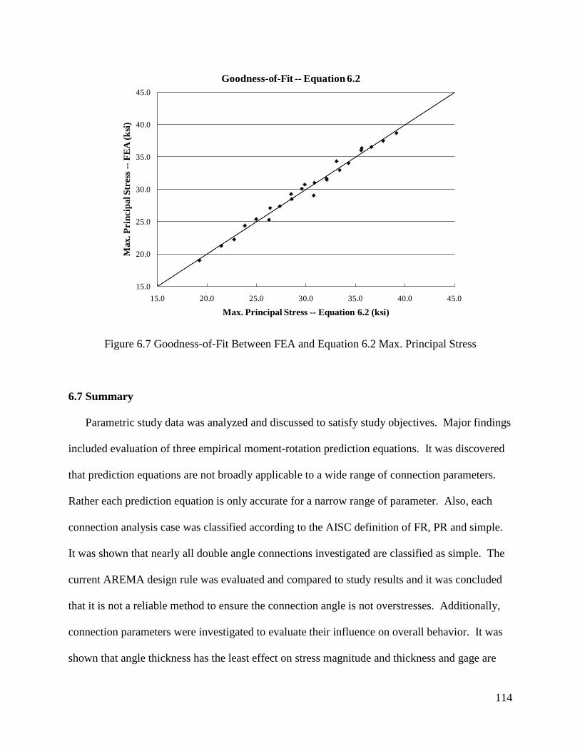
114
Figure 6.7 Goodness-of-Fit Between FEA and Equation 6.2 Max. Principal Stress
6.7 Summary
Parametric study data was analyzed and discussed to satisfy study objectives. Major findings
included evaluation of three empirical moment-rotation prediction equations. It was discovered
that prediction equations are not broadly applicable to a wide range of connection parameters.
Rather each prediction equation is only accurate for a narrow range of parameter. Also, each
connection analysis case was classified according to the AISC definition of FR, PR and simple.
It was shown that nearly all double angle connections investigated are classified as simple. The
current AREMA design rule was evaluated and compared to study results and it was concluded
that it is not a reliable method to ensure the connection angle is not overstresses. Additionally,
connection parameters were investigated to evaluate their influence on overall behavior. It was
shown that angle thickness has the least effect on stress magnitude and thickness and gage are
15.0
20.0
25.0
30.0
35.0
40.0
45.0
15.0 20.0 25.0 30.0 35.0 40.0 45.0
Max
. Pri
ncip
al S
tres
s --F
EA
(ksi
)
Max. Principal Stress -- Equation 6.2 (ksi)
Goodness-of-Fit -- Equation 6.2

115
proportional to stress while the stress-length relationship is nonlinear. Lastly, the following
quadratic stress prediction equation was proposed that is a function of L, t, and g.
0.1503.78.177.11424.0 2max_ −−−+−= gtLLpσ (6.4)
Equation 6.4 provides a satisfactory level of accuracy with a coefficient of correlation, r equal to
0.992. This stress equation rapidly and effectively predicts the magnitude of stress range, SR for
the 286,000 pound GCW fatigue vehicle. Subsequently, fatigue life is easily evaluated according
to AREMA (2008a) with estimated number of cycles to failure, N computed with the following
equation when SR exceeds the threshold stress, STH :
0.3−= RASN (6.5)
where A is a constant depending on fatigue detail category. Recalling from Chapter 2 that
fatigue category A applies for the base metal of the connection angle; A=2.5×10¹⁰ and STH = 24
ksi. The relationship of equation 6.5 represents the SR-N curve presented in Figure 2.3.

116
Chapter 7
SUMMARY AND CONCLUSIONS
7.1 Summary
Double angle stringer-to-floorbeam connections in girder-floorbeam-stringer bridges are
recognized as fatigue prone details due to stress induced by stringer end rotation from live load.
Distortion induced, secondary stress is not directly accounted for in design and is not easily
calculable. Many bridges containing this detail are nearing the end or functioning past their
design life, especially on railways. As bridge owners and managers seek to preserve the value
and function of their assets by continuing to extend bridge lives, fatigue damage is a concern.
The primary goal of this research was to investigate distortion induced stress in double angle
connections and propose an easy and effective stress prediction method to facilitate fatigue
evaluation without the need for a rigorous analysis.
A parametric study framework was presented in Chapter 3 to evaluate double angle
connection behavior considering primary parameters: stringer length, L angle thickness, t angle
depth, d and outstanding leg gage, g. The study was limited in scope to riveted connections in
typical girder-floorbeam-stringer railway bridges with a fatigue vehicle defined as a standard
286,000 pound GCW plus impact loading. Parameter combinations defined 72 unique analysis
cases that were investigated through a combination of 2D and 3D FEA. Experimental evaluation
of two laboratory test specimens was presented in Chapter 4. The experimental study provided
comparison data for 3D FE model verification. Numerical modeling and analysis was presented
and discussed in detail in Chapter 5.
117
Numerical modeling consisted of 3D FEA with ABAQUS version 6.9 and 2D FEA with
SAP2000 version 14. Service range moment-rotation behavior for each analysis case was
predicted by 3D FEA. Initial secant stiffness, Ks of the connection was calculated from the
resulting nonlinear moment-rotation curve with an assumed magnitude for service end moment,
Ms. The magnitude of Ks was used to define linear spring supports in a companion 2D stringer
beam FE model. This model was loaded with the defined fatigue vehicle and the resulting Ms
was compared with the initially assumed value. A new Ks was computed and iteration was
performed until Ms values converged. The state of stress in the angle of the 3D FE model
corresponding to Ms was then investigated. It was observed in all analysis cases that maximum
principal stress occurred at the toe of the fillet on the stringer leg of the angle, even with the top
fasteners. Moment-rotation and maximum principal stress results were presented in Chapter 5
followed by analyses and discussion in Chapter 6.
Parametric study results were analyzed and discussed according to research objectives.
Three empirical moment-rotation prediction equations were evaluated and compared to 3D FEA
predictions. Also, each connection was classified according to AISC definitions of FR, PR, and
simple. The current AREMA design rule, developed in 1939, was evaluated to determine its
effectiveness in minimizing connection angle stress. Additionally, connection parameters were
investigated to evaluate their influence on overall load response behavior. Finally, linear
regression analysis was used to develop a stress prediction equation as a function of study
parameters. This equation effectively predicts the magnitude of stress induced in connection
angles from the 286,000 pound fatigue vehicle without the need for vigorous analysis.
Consequently, this facilitates fatigue life evaluation for double angle connection details.

118
7.2 Conclusions
The following main conclusions are made from the presented parametric study research.
Empirical moment-rotation prediction equations are not broadly applicable to typical double
angle connection configurations used in railroad bridges. Moment-rotation for stiff connections
with g = 2.0 inches is best predicted with the Kishi and Chen equation. Frye and Morris
equation approximately represents moment-rotation for connections with 2.0 ≤ g ≤ 2.5 inches.
The Attiogbe and Morris equation is more suitable for flexible connections when d > 10 inches
and g ≥ 3.0 inches. Compared to FEA, these equations provide approximate moment-rotation
relationship for a limited range of connection parameters. It is concluded that, in a general sense,
these empirical equations do not reliably predict moment-rotation and should not be used as a
stand-alone method in design or analysis.
Stringer beam design assumes double angle connections act as simple supports, resisting only
shear force. It has been shown that these connections provide some rotational restraint in the
form of end moment. According to the AISC definition for FR, PR and simple, each of the 72
analysis cases were classified. It was shown that 67 of 72 connections classify as simple and the
remaining 5 narrowly exceed the simple threshold and are therefore classified as PR. For
stringer beam design, it is concluded that assuming double angle connections to act as simple
supports is valid.
The current AREMA design rule, proposed by Wilson (1939) and presented in equation 1.1
was evaluated and compared to parametric study results. According to Wilson (1939) this

119
relationship between L, t, and g with K=8 ensures adequate flexibility in the angle such that they
are not overstressed by distortion induced stresses. This implies that connection flexibility is
inversely related to stress. Considering Ks as a measure of flexibility, no observable relationship
between connection flexibility and stress is observed from Figure 6.5. This seems
counterintuitive because for many structural engineering problems, there is correlation between
stiffness and stress. However, in the case of double angle connections, connection stiffness was
not constant as observed by the nonlinear moment-rotation curves. It was also observed that:
• as t increased, Ks increased but σp_max decreased;
• as g increased, both Ks and σp_max increased;
Additionally, stringer stiffness influenced connection behavior which ultimately had an effect on
stiffness and stress. Based on these observations it is sensible that a correlation does not exist
between connection stiffness and stress.
Variation in design constant, K has little effect on Ks as observed from Figure 6.4.
Consequently, from Figure 6.6 it can be concluded that satisfying equation 1.1 (when K ≤ 8), has
practically no effect on the magnitude of stress. It is therefore concluded that equation 1.1 does
not ensure connection angles are not overstressed. Moreover, when considering equal magnitude
live loading (in this case 286,000 pound GCW) stiffness and stress are not related.
Maximum principal stress relationships, as a function of parameters L, t, g and d, were
investigated. It can be concluded that maximum principal stress does not vary significantly with
d and is inversely proportional to g and t. Additionally, maximum principal stress increases
nonlinearly with L. It was also shown that Ks increased with t, but decreased with increased g.
Linear regression analysis was performed to quantify maximum principal stress as a function of

120
L, t, and g. The proposed stress prediction equation 6.4 provides a very good fit to numerical
results as indicated with r =0.992 indicates. It is concluded that equation 6.4 provides an
effective method to reliably estimate the service stress range, SR for the 286,000 pound GCW to
facilitate rapid fatigue life evaluation.
7.3 Recommendations for Future Research
The present study relied entirely on numerical results with limited experimental laboratory
verification testing. A major assumption in numerical modeling was a fixed boundary surface
representing the floorbeam web. The proposed stress prediction equation provides a very good
fit to numerical data, however accuracy compared to field data has not been tested. There is a
need for further research to collect 286, 000 pound GCW live load field data to evaluate the true
accuracy of equation 6.4. It is expected a modifying parameter, or reliability factor must be
considered to account for variability in real field conditions.
Additionally, the present study is limited in scope. There is a need to expand the scope to
include variable load magnitude. The 286,000 pound GCW is the maximum equipment load on
most freight railways. Therefore, with respect to fatigue, it has the most damaging effect.
However, not all freight equipment loads out at 286,000 pounds and some railroads are capable
of handling heavier axle loads. Fatigue is the accumulation of load cycles of all magnitudes.
Accounting for load magnitude in a stress prediction equation is necessary to predict all load
history.
Finally, it has been shown that double angle connection behavior is dependent on the
stiffness of the connected stringer. Therefore variable stringer stiffness should be considered.
The present study assumed a stringer section modulus based on E-80 design loading and nominal

121
depth. Limited field observations [Laman and Guyer, 2010] indicated that not all stringers are
adequate for the E-80 design load.

122
Appendix: RESULTS – TABLES AND GRAPHS
Table A-1 (a) Maximum Principal Stress - Analysis Cases 1 – 36
Angle Thickness, t
Stringer Length, L
Gage Distance, g
Angle Depth, d
Secant Stiffness, K s
Service End Moment, M s
Maximum Principal Stress, σ p_max
inches feet inches inches k-ft/rad k-ft ksi1 10 11900 14.6 312 11.5 22700 20.1 303 13 26900 20.4 274 10 7850 11.0 275 11.5 14900 16.0 266 13 17400 15.9 237 10 5530 8.3 228 11.5 9690 11.7 229 13 12100 12.3 2010 10 10700 20.4 3811 11.5 20300 28.9 3512 13 23600 29.6 3613 10 7440 15.6 3614 11.5 13600 22.1 3515 13 16700 23.2 3216 10 5300 11.9 3117 11.5 9370 16.8 3018 13 11100 17.8 3019 11.5 12200 25.4 3820 13 14800 26.9 3721 14.5 25400 35.4 3822 11.5 8570 19.3 3423 13 11200 21.1 3324 14.5 17300 27.2 3525 11.5 6430 14.8 2926 13 8170 16.2 2827 14.5 12200 20.9 3128 13 15100 29.4 3829 14.5 23200 38.2 4030 16 32900 45.2 3931 13 10400 22.5 3632 14.5 16200 29.4 3733 16 22700 34.1 3634 13 7750 17.4 3035 14.5 11600 22.5 3436 16 16900 27.0 30
Eqn 1.1 Constant,
K
12.0
7.7
5.3
15.0
9.6
6.9
3.0 6.7
11.5
3.0
3.5
2.5
3.0
8.0
5.9
13.4
9.3
3.5
2.5
2.0
2.5
3.0
2.0
2.5
Analysis Case
Number
1/2
8
10
12
14

123
Table A-1(b) Maximum Principal Stress - Analysis Cases 37-72
Angle Thickness, t
Stringer Length, L
Gage Distance, g
Angle Depth, d
Secant Stiffness, K s
Service End Moment, M s
Maximum Principal Stress, σ p_max
inches feet inches inches k-ft/rad k-ft ksi37 10 18000 19.0 2838 11.5 36200 25.2 2639 13 41600 25.3 2240 10 12900 15.4 2341 11.5 24400 20.8 2442 13 28700 21.1 2043 10 9460 12.3 1944 11.5 16700 16.8 2045 13 20300 17.4 1846 10 11800 22.0 3147 11.5 21600 30.2 3348 13 26900 31.3 2849 10 8290 17.5 2850 11.5 15600 24.2 2851 13 18300 25.4 2652 10 6330 14.1 2553 11.5 11200 19.6 2554 13 14200 20.9 2355 11.5 21200 36.1 3656 13 24700 37.3 3357 14.5 41600 47.7 3958 11.5 15000 28.9 3259 13 17500 30.2 3160 14.5 29000 39.1 3261 11.5 11000 23.1 2962 13 13600 24.7 2763 14.5 21100 31.7 3064 13 17600 33.2 3265 14.5 28000 43.1 3566 16 39900 50.2 3267 13 13000 26.8 3068 14.5 20600 34.8 3269 16 29100 43.2 3170 13 10200 21.7 2671 14.5 15100 27.9 2872 16 21400 33.0 27
7.3
10.0
Eqn 1.1 Constant,
K
15.0
14.4
6.1
8.3
12.0
6.7
9.6
3
3.5
4
2.5
3
3.5
2.5
3
3.5
6.6
8.6
11.7
5/8
8
10
12
14
2
2.5
3
Analysis Case
Number

124
Moment-Rotation Prediction Comparison for Angle Depth, d=10”
BLANK
Figure A-1 Moment-Rotation Prediction Comparison for Angle Depth, d=10”
0
5
10
15
20
25
30
0.000 0.001 0.002 0.003 0.004 0.005
Mom
ent (
k-ft
)
Rotation (radians)
t=0.5'', g=2'', d=10''
0
5
10
15
20
25
30
0.000 0.001 0.002 0.003 0.004 0.005
Mom
ent (
k-ft
)
Rotation (radians)
t=0.625'', g=2'', d=10''
0
5
10
15
20
25
30
0.000 0.001 0.002 0.003 0.004 0.005
Mom
ent (
k-ft
)
Rotation (radians)
t=0.5'', g=2.5'', d=10''
0
5
10
15
20
25
30
0.000 0.001 0.002 0.003 0.004 0.005
Mom
ent (
k-ft
)
Rotation (radians)
t=0.625'', g=2.5'', d=10''
0
5
10
15
20
25
30
0.000 0.001 0.002 0.003 0.004 0.005
Mom
ent (
k-ft
)
Rotation (radians)
t=0.5'', g=3'', d=10''
0
5
10
15
20
25
30
0.000 0.001 0.002 0.003 0.004 0.005
Mom
ent (
k-ft
)
Rotation (radians)
t=0.625'', g=3'', d=10''
0
5
10
15
20
25
30
0.000 0.001 0.002 0.003 0.004 0.005
Mom
ent (
k-ft
)
Rotation (radians)
t=0.625'', g=3.5'', d=10''
Frye & Morris Attiogbe & Morris Kishi & Chen 3D FEA

125
Moment-Rotation Prediction Comparison for Angle Depth, d=11.5”
Figure A-2 Moment-Rotation Prediction Comparison for Angle Depth, d=11.5”
0
5
10
15
20
25
30
35
0.000 0.001 0.002 0.003 0.004 0.005
Mom
ent (
k-ft
)
Rotation (radians)
t=0.5'', g=2'', d=11.5''
0
5
10
15
20
25
30
35
0.000 0.001 0.002 0.003 0.004 0.005
Mom
ent (
k-ft
)
Rotation (radians)
t=0.625'', g=2'', d=11.5''
0
5
10
15
20
25
30
35
0.000 0.001 0.002 0.003 0.004 0.005
Mom
ent (
k-ft
)
Rotation (radians)
t=0.5'', g=2.5'', d=11.5''
0
5
10
15
20
25
30
35
0.000 0.001 0.002 0.003 0.004 0.005
Mom
ent (
k-ft
)
Rotation (radians)
t=0.625'', g=2.5'', d=11.5''
0
5
10
15
20
25
30
35
0.000 0.001 0.002 0.003 0.004 0.005
Mom
ent (
k-ft
)
Rotation (radians)
t=0.5'', g=3'', d=11.5''
0
5
10
15
20
25
30
35
0.000 0.001 0.002 0.003 0.004 0.005
Mom
ent (
k-ft
)
Rotation (radians)
t=0.625'', g=3'', d=11.5''
0
5
10
15
20
25
30
35
0.000 0.001 0.002 0.003 0.004 0.005
Mom
ent (
k-ft
)
Rotation (radians)
t=0.5'', g=3.5'', d=11.5''
0
5
10
15
20
25
30
35
0.000 0.001 0.002 0.003 0.004 0.005
Mom
ent (
k-ft
)
Rotation (radians)
t=0.625'', g=3.5'', d=11.5''
Frye & Morris Attiogbe & Morris Kishi & Chen 3D FEA

126
Moment-Rotation Prediction Comparison for Angle Depth, d=13”
Figure A-3 (a) Moment-Rotation Prediction Comparison for Angle Depth, d=13”
0
5
10
15
20
25
30
35
0.000 0.001 0.002 0.003 0.004 0.005
Mom
ent (
k-ft
)
Rotation (radians)
t=0.5'', g=2'', d=13''
0
5
10
15
20
25
30
35
0.000 0.001 0.002 0.003 0.004 0.005
Mom
ent (
k-ft
)
Rotation (radians)
t=0.625'', g=2'', d=13''
0
5
10
15
20
25
30
35
0.000 0.001 0.002 0.003 0.004 0.005
Mom
ent (
k-ft
)
Rotation (radians)
t=0.5'', g=2.5'', d=13''
0
5
10
15
20
25
30
35
0.000 0.001 0.002 0.003 0.004 0.005
Mom
ent (
k-ft
)
Rotation (radians)
t=0.625'', g=2.5'', d=13''
0
5
10
15
20
25
30
35
0.000 0.001 0.002 0.003 0.004 0.005
Mom
ent (
k-ft
)
Rotation (radians)
t=0.5'', g=3'', d=13''
0
5
10
15
20
25
30
35
0.000 0.001 0.002 0.003 0.004 0.005
Mom
ent (
k-ft
)
Rotation (radians)
t=0.625'', g=3'', d=13''
0
5
10
15
20
25
30
35
0.000 0.001 0.002 0.003 0.004 0.005
Mom
ent (
k-ft
)
Rotation (radians)
t=0.5'', g=3.5'', d=13''
0
5
10
15
20
25
30
35
0.000 0.001 0.002 0.003 0.004 0.005
Mom
ent (
k-ft
)
Rotation (radians)
t=0.625'', g=3.5'', d=13''
Frye & Morris Attiogbe & Morris Kishi & Chen 3D FEA

127
Moment-Rotation Prediction Comparison for Angle Depth, d=13” (con’t)
BLANK
Figure A-3 (b) Moment-Rotation Prediction Comparison for Angle Depth, d=13”
0
5
10
15
20
25
30
35
0.000 0.001 0.002 0.003 0.004 0.005
Mom
ent (
k-ft
)
Rotation (radians)
t=0.625'', g=4'', d=13''
Frye & Morris Attiogbe & Morris Kishi & Chen 3D FEA

128
Moment-Rotation Prediction Comparison for Angle Depth, d=14.5”
BLANK
Figure A-4 Moment-Rotation Prediction Comparison for Angle Depth, d=14.5”
05
101520253035404550
0.000 0.001 0.002 0.003 0.004 0.005
Mom
ent (
k-ft
)
Rotation (radians)
t=0.5'', g=2.5'', d=14.5''
05
101520253035404550
0.000 0.001 0.002 0.003 0.004 0.005
Mom
ent (
k-ft
)
Rotation (radians)
t=0.625'', g=2.5'', d=14.5''
05
101520253035404550
0.000 0.001 0.002 0.003 0.004 0.005
Mom
ent (
k-ft
)
Rotation (radians)
t=0.5'', g=3'', d=14.5''
05
101520253035404550
0.000 0.001 0.002 0.003 0.004 0.005
Mom
ent (
k-ft
)
Rotation (radians)
t=0.625'', g=3'', d=14.5''
05
101520253035404550
0.000 0.001 0.002 0.003 0.004 0.005
Mom
ent (
k-ft
)
Rotation (radians)
t=0.5'', g=3.5'', d=14.5''
05
101520253035404550
0.000 0.001 0.002 0.003 0.004 0.005
Mom
ent (
k-ft
)
Rotation (radians)
t=0.625'', g=3.5'', d=14.5''
05
101520253035404550
0.000 0.001 0.002 0.003 0.004 0.005
Mom
ent (
k-ft
)
Rotation (radians)
t=0.625'', g=4'', d=14.5''
Frye & Morris Attiogbe & Morris Kishi & Chen 3D FEA

129
Moment-Rotation Prediction Comparison for Angle Depth, d=16”
BLANK
BLANK
Figure A-5 Moment-Rotation Prediction Comparison for Angle Depth, d=16”
05
101520253035404550
0.000 0.001 0.002 0.003 0.004 0.005
Mom
ent (
k-ft
)
Rotation (radians)
t=0.5'', g=2.5'', d=16''
05
101520253035404550
0.000 0.001 0.002 0.003 0.004 0.005
Mom
ent (
k-ft
)
Rotation (radians)
t=0.5'', g=3'', d=16''
05
101520253035404550
0.000 0.001 0.002 0.003 0.004 0.005
Mom
ent (
k-ft
)
Rotation (radians)
t=0.625'', g=3'', d=16''
05
101520253035404550
0.000 0.001 0.002 0.003 0.004 0.005
Mom
ent (
k-ft
)
Rotation (radians)
t=0.5'', g=3.5'', d=16''
05
101520253035404550
0.000 0.001 0.002 0.003 0.004 0.005
Mom
ent (
k-ft
)
Rotation (radians)
t=0.625'', g=3.5'', d=16''
05
101520253035404550
0.000 0.001 0.002 0.003 0.004 0.005
Mom
ent (
k-ft
)
Rotation (radians)
t=0.625'', g=4'', d=16''
Frye & Morris Attiogbe & Morris Kishi & Chen 3D FEA

130
Table A-2 (a) Moment-Rotation Prediction Equation – Ks Comparison -- Analysis Cases 1-36
Angle Thickness, t
Stringer Length, L
Gage Distance, g
Angle Depth, d
Secant Stiffness, K s
Frye-Morris Eqn.
Attiogbe-Morris Eqn.
Kishi-Chen Eqn.
inches feet inches inches k-ft/rad1 10 11900 5% 164% 3%2 11.5 22700 25% 128% 11%3 13 26900 11% 152% 10%4 10 7850 45% 134% 28%5 11.5 14900 15% 78% 53%6 13 17400 30% 114% 39%7 10 5530 75% 97% 57%8 11.5 9690 55% 18% 73%9 13 12100 62% 68% 63%
10 10 10700 11% 161% 11%11 11.5 20300 20% 122% 25%12 13 23600 1% 147% 3%13 10 7440 47% 132% 34%14 11.5 13600 21% 71% 56%15 13 16700 32% 111% 47%16 10 5300 78% 94% 56%17 11.5 9370 57% 16% 73%18 13 11100 69% 61% 58%19 11.5 12200 30% 62% 54%20 13 14800 43% 104% 45%21 14.5 25400 15% 56% 66%22 11.5 8570 64% 10% 67%23 13 11200 68% 62% 61%24 14.5 17300 52% 1% 72%25 11.5 6430 88% 30% 94%26 13 8170 93% 15% 88%27 14.5 12200 82% 40% 96%28 13 15100 40% 105% 49%29 14.5 23200 24% 49% 64%30 16 32900 13% 3% 74%31 13 10400 74% 56% 55%32 14.5 16200 58% 2% 68%33 16 22700 49% 38% 73%34 13 7750 97% 11% 84%35 14.5 11600 86% 38% 92%36 16 16900 74% 54% 101%
Analysis Case
Number
1/2
8
10
12
14
2.0
2.5
3.0
2.0
2.5
6.7
11.5
3.0
3.5
2.5
15.0
9.6
6.9
3.0
3.0
8.0
5.9
13.4
9.3
3.5
2.5
percent difference in calculated K s
Eqn 1.1 Constant,
K
12.0
7.7
5.3

131
Table A-2 (b) Moment-Rotation Prediction Equation – Ks Comparison --Analysis Cases 37-72
Angle Thickness, t
Stringer Length, L
Gage Distance, g
Angle Depth, d
Secant Stiffness, K s
Frye-Morris
Attiogbe-Morris Kishi-Chen
inches feet inches inches k-ft/rad37 10 18000 6% 172% 17%38 11.5 36200 30% 146% 4%39 13 41600 14% 164% 27%40 10 12900 37% 152% 40%41 11.5 24400 7% 107% 62%42 13 28700 21% 137% 44%43 10 9460 64% 125% 50%44 11.5 16700 42% 58% 67%45 13 20300 52% 100% 55%46 10 11800 42% 149% 48%47 11.5 21600 16% 98% 68%48 13 26900 26% 133% 53%49 10 8290 74% 117% 44%50 11.5 15600 47% 52% 66%51 13 18300 60% 93% 52%52 10 6330 95% 83% 69%53 11.5 11200 76% 3% 87%54 13 14200 82% 54% 79%55 11.5 21200 16% 97% 73%56 13 24700 33% 128% 55%57 14.5 41600 7% 87% 67%58 11.5 15000 49% 49% 66%59 13 17500 64% 89% 51%60 14.5 29000 41% 35% 69%61 11.5 11000 77% 3% 86%62 13 13600 85% 50% 76%63 14.5 21100 70% 10% 89%64 13 17600 63% 90% 54%65 14.5 28000 44% 33% 68%66 16 39900 34% 12% 75%67 13 13000 88% 47% 74%68 14.5 20600 71% 9% 87%69 16 29100 62% 31% 94%70 13 10200 106% 8% 94%71 14.5 15100 96% 34% 103%72 16 21400 87% 49% 109%
Analysis Case
Number
5/8
8
10
12
14 3.5
4
2.5
3
3.5
2.5
3
3.5
6.6
8.6
11.73
2
2.5
3
percent difference in calculated K s
7.3
10.0
Eqn 1.1 Constant,
K
15.0
14.4
6.1
8.3
12.0
6.7
9.6

132
Connection Classification for 286,000 lb GCW Fatigue Load
Figure A-6 Connection Classification (a) Stringer Length, L= 8’, 10’
0
5
10
15
20
25
30
35
40
45
50
0 0.001 0.002 0.003 0.004
Mom
ent (
k-ft
)
Rotation (radians)
L=8', d=10" (I=472in4)
t=0.5", g=2.0"t=0.5", g=2.5"t=0.5", g=3.0"t=0.625", g=2.0"t=0.625", g=2.5"t=0.625", g=3.0"
SIMPLE
PR
FR
0
5
10
15
20
25
30
35
40
45
50
0 0.001 0.002 0.003 0.004
Mom
ent (
k-ft
)
Rotation (radians)
L=10', d=10" (I=472in4)
t=0.5", g=2.0"t=0.5", g=2.5"t=0.5", g=3.0"t=0.625", g=2.5"t=0.625", g=3.0"t=0.625", g=3.5"
SIMPLE
PR
FR
0
5
10
15
20
25
30
35
40
45
50
0 0.001 0.002 0.003 0.004
Mom
ent (
k-ft
)
Rotation (radians)
L=8', d=11.5" (I=543in4)
t=0.5", g=2.0"t=0.5", g=2.5"t=0.5", g=3.0"t=0.625", g=2.0"t=0.625", g=2.5"t=0.625", g=3.0"
SIMPLE
PR
FR
0
5
10
15
20
25
30
35
40
45
50
0 0.001 0.002 0.003 0.004
Mom
ent (
k-ft
)
Rotation (radians)
L=10', d=11.5" (I=543in4)
t=0.5", g=2.0"t=0.5", g=2.5"t=0.5", g=3.0"t=0.625", g=2.5"t=0.625", g=3.0"t=0.625", g=3.5"
SIMPLE
PR
FR
0
5
10
15
20
25
30
35
40
45
50
0 0.001 0.002 0.003 0.004
Mom
ent (
k-ft
)
Rotation (radians)
L=8', d=13" (I=613in4)
t=0.5", g=2.0"t=0.5", g=2.5"t=0.5", g=3.0"t=0.625", g=2.0"t=0.625", g=2.5"t=0.625", g=3.0"
SIMPLE
PR
FR
0
5
10
15
20
25
30
35
40
45
50
0 0.001 0.002 0.003 0.004
Mom
ent (
k-ft
)
Rotation (radians)
L=10', d=13" (I=613in4)
t=0.5", g=2.0"t=0.5", g=2.5"t=0.5", g=3.0"t=0.625", g=2.5"t=0.625", g=3.0"t=0.625", g=3.5"
SIMPLE
PR
FR

133
Connection Classification for 286,000 lb GCW Fatigue Load
Figure A-6 Connection Classification (b) Stringer Length, L= 12’, 14’
0
5
10
15
20
25
30
35
40
45
50
0 0.001 0.002 0.003 0.004
Mom
ent (
k-ft
)
Rotation (radians)
L=12', d=11.5" (I=543in4)
t=0.5", g=2.5"t=0.5", g=3.0"t=0.5", g=3.5"t=0.625", g=2.5"t=0.625", g=3.0"t=0.625", g=3.5"
SIMPLE
PR
FR
0
5
10
15
20
25
30
35
40
45
50
0 0.001 0.002 0.003 0.004
Mom
ent (
k-ft
)
Rotation (radians)
L=14', d=13" (I=613in4)
t=0.5", g=2.5"t=0.5", g=3.0"t=0.5", g=3.5"t=0.625", g=3.0"t=0.625", g=3.5"t=0.625", g=4.0"
SIMPLE
PR
FR
0
5
10
15
20
25
30
35
40
45
50
0 0.001 0.002 0.003 0.004
Mom
ent (
k-ft
)
Rotation (radians)
L=12', d=13" (I=613in4)
t=0.5", g=2.5"t=0.5", g=3.0"t=0.5", g=3.5"t=0.625", g=2.5"t=0.625", g=3.0"t=0.625", g=3.5"
SIMPLE
PR
FR
0
5
10
15
20
25
30
35
40
45
50
0 0.001 0.002 0.003 0.004
Mom
ent (
k-ft
)
Rotation (radians)
L=14', d=14.5" (I=1368in4)
t=0.5", g=2.5"t=0.5", g=3.0"t=0.5", g=3.5"t=0.625", g=3.0"t=0.625", g=3.5"t=0.625", g=4.0"
SIMPLE
PR
FR
0
5
10
15
20
25
30
35
40
45
50
0 0.001 0.002 0.003 0.004
Mom
ent (
k-ft
)
Rotation (radians)
L=12', d=14.5" (I=1368in4)
t=0.5", g=2.5"t=0.5", g=3.0"t=0.5", g=3.5"t=0.625", g=2.5"t=0.625", g=3.0"t=0.625", g=3.5"
SIMPLE
PR
FR
0
5
10
15
20
25
30
35
40
45
50
0 0.001 0.002 0.003 0.004
Mom
ent (
k-ft
)
Rotation (radians)
L=14', d=16" (I=2076in4)
t=0.5", g=2.5"t=0.5", g=3.0"t=0.5", g=3.5"t=0.625", g=3.0"t=0.625", g=3.5"t=0.625", g=4.0"
SIMPLE
PR
FR

134
Bibliography
ABAQUS Analysis User’s Manual. (2009). Dassault Systèmes Simulia Corp., Providence, RI. Al-Emrani, M. (2005). “Fatigue Performance of Stringer-to-Floor-Beam Connections in Riveted Railway Brdiges.” J. Bridge Eng., ASCE, 10(2), 179-185. Al-Emrani, M., Kliger, R. (2003). “FE Analysis of Stringer-to-Floor-Beam Connections in Riveted Railway Bridges.” J. Constr. Steel Res., 59(7), 803-818. American Railway Engineering and Maintenance-of-Way Association. (2008a). “Steel Bridges.” Manual for Railway Engineering, Ch 15. American Railway Engineering and Maintenance-of-Ways Association. (2008b). “AREMA Bridge Inspection Handbook.” AREMA, Lanham MD. American Institute of Steel Construction (AISC). (2005). “Steel Construction Manual.” 13th Edition. Astaneh, A., Nader, M.N., Makil, L. (1989). “Cyclic Behavior of Double Angle Connections.” J. Struct. Eng., ASCE, 115(5), 1101-1117. Attiogbe, E., Morris, G. (1991). “Moment-Rotation Functions for Steel Connections.” J. Struct. Eng., ASCE, 117(6),1703-1718. Byers, W.G., Marley, M.J., Mohammadi, J., Nielsen, R.J., Sarkani, S. (1997). “Fatigue Reliability Reassessment Proceedures: State-of-the Art Paper.” J. Struct. Eng., ASCE, 123(3), 271-276. Byers, W.G., Marley, M.J., Mohammadi, J., Nielsen, R.J., Sarkani, S. (1997). “Fatigue Reliability Reassessment Applications: State-of-the Art Paper.” J. Struct. Eng., ASCE, 123(3), 277-285. Byers, W.G. (1992). “History of Railway Bridge Loading.” Chen, W.F. (2000). Practical Analysis for Semi-Rigid Frame Design, World Scientific Publishing Co., Singapore. CSI Analysis Reference Manual for SAP2000. (2007). Computer and Structures Inc., Berkeley, CA. DePiero, A.H., Paasch, R.K., Lovejoy, S.C. (2002). “Finite-Element Modeling of Bridge Deck Connection Details.” J. Bridge Eng., ASCE, 7(4), 229-235.

135
DiBattista, J.D., Adamson, D.E., Kulak, G. (1998). “Fatigue Strength of Riveted Connections.” J. Struct. Eng., ASCE, 124(7), 792-797. Dick, S.M., ( ). “Fatigue Loading Behavior of General Mixed Freight Traffic.” Dick, S.M., Otter, D., Joy, R.B., Akhtar, M.N. (2008). “Girder Fatigue Modeling: Actual Verses Theoretical.” Proc., AREMA. Faella, C., Piluso, V., Rizzano, G. (2000.) Structural Steel Semirigid Connections, CRC Press LLC, Boca Raton, Florida. Fisher, J.W., Jin, J., Wagner, D.C., Yen, B.T. (1990a). “Distortion-Induced Fatigue Cracking in Steel Bridges.” Transp. Res. Board, NCHRP Rep. No. 336, Nat. Res. Council, Washington D.C. Fisher, J.W., Yen, B.T., Wang, D. (1990b). “Fatigue Strength of Riveted Bridge Members.” J. Struct. Eng., ASCE, 116(11), 2968-2981. Fisher, J.W., Yen, B.T., Wang, D, Mann, J.E. (1987). “Fatigue and Fracture Evaluation for Rating Riveted Bridges.” Transp. Res. Board, NCHRP Rep. No. 302, Nat. Res. Council, Washington D.C. Hong, K., Yang, J.G., Lee, S.K. (2001). “Moment-Rotation Behavior of Double Angle Connections Subjected to Shear Load.” Eng. Struct., 24, 125-132. Imam, B.M., Righiniotis, T.D., Chryssanthopoulos, M.K. (2007). “Numerical Modeling of Riveted Railway Bridge Connections for Fatigue Evaluation.” Eng. Struct., 29(11), 3071-3081. Imam, B.M., Righiniotis, T.D., Chryssanthopoulos, M.K. (2008). “Fatigue Analysis of Riveted Railway Bridge Connections Using the Theory of Critical Distances.” Eng. Struct., 30(10), 2707-2715. Kim Roddis, W.M., Zhao, Y. (2003). “Finite-Element Analysis of Steel Bridge Distortion-Induced Fatigue.” J. Bridge Eng., ASCE, 8(5), 259-266. Kishi, N., Chen, W. (1990). “Moment-Rotation Relations of Semirigid Connections with Angles.” J. Struct. Eng., ASCE, 116(7), 1813-1834. Kulak, G.L. (2000). “Fatigue Strength of Riveted Shear Splices.” Prog. Struct. Engng. Mater., 2, 110-119. Kulak, G.L., Fisher, J.W., Struik, J.H.A. (2001). “Guide to Design Criteria for Bolted and Riveted Joints.” Second Edition, AISC, Chicago, Ill.

136
Laman, J.A., Guyer, R.C. (2010). “Condition Assessment of Short-line Railroad Bridges in Pennsylvania.” Pennsylvania Transportation Institute: PennDOT Research Report (FHWA-PA-2010-003-PSU 022), The Pennsylvania State University, University Park, PA. Laman, J.A., Leighty, C., Gittings, G.L., Erdogmus, E., Boothby, T.E. (2001). “Heavy Axle Study: Impact of Higher Rail Car Weight Limits on Short-Line Railroads, Vol. I & II.” Pennsylvania Transportation Institute: PennDOT Research Report (359704), The Pennsylvania State University, University Park, Pa. Otter, D., Akhtar, M.N., Doe, B., Yoshino, D. (2006). “Crack Development and Growth in the FAST Steel Bridge.” Proc., AREMA. Philbriek, T.W., Zodo, G.W., Schiff, S.D. (1995). “Fatigue Assessment of Through Plate Girder Railway Bridges.” J. Struct. Eng., ASCE, 121(11), 1613-1619. Roeder, C.W., MacRae, G., Leland, A., Rospo, A. (2005). “Extending the Fatigue Life of Riveted Coped Stringer Connections.” J. Bridge Eng., ASCE, 10(1), 69-75. Roeder, C.W., MacRae, G.A., Arima, K., Crocker, P.N., Wong, S.D. (1998). “Fatigue Cracking of Riveted Steel Tied Arch and Truss Bridges.” Rep. No. WA-RD447.1, Washington Department of Transportation, Olympia, Wash. Salmon, Charles G., Johnson, John E., Malhas, Faris A. (2009). Steel Structures Behavior and Design. Pearson-Prentice Hall, Upper Saddle River, New Jersey. Shakoor Uppal, A. (2005). “Coping With the Older Railroad Steel Bridges.” Proc., AREMA. Tamboli, A. (2010). Handbook of Structural Steel Connection Design and Details. McGraw-Hill Companies, Inc., New York. Tobias, D.H., Foutch, D.A. (1997). “Reliability-Based Method for Fatigue Evaluation of Railway Bridges.” J. Bridge Eng., ASCE, 2(2), 53-60. Wilson, W.M. (1940). “Design of Connection Angles for Stringers of Railway Bridges.” Proc., AREA, 41, 889-903. Wilson, W.M., Coombe, J.W. (1939). “Fatigue Tests of Connection Angles.” Eng. Experiment Station Bulletin, University of Illinois, 317(6).