- 1 -

DISTRIBUTED DATABASES FUNDAMENTALS AND RESEARCH

Haroun Rababaah

Advanced Database – B561. Spring 2005. Dr. H. Hakimzadeh

Department of Computer and Information Sciences Indiana University South Bend

ABSTRACT The purpose of this paper is to present an introduction to distributed databases though two main parts: in the first part, we present a study of the fundamentals of distributed databases (DDBS). We discuss issues related to the motivations of DDBS, architecture, design, performance, and concurrency control, etc. In the second part, we explore some of the research that has been done in this specific area of DDBS. The topics of this research include, query optimization, distribution optimization, fragmentation, optimization, and join optimization on the internet. We include examples and results to demonstrate the topics we are presenting. KEYWORDS Distributed databases fundamentals, current research: query optimization, distribution optimization, fragmentation optimization, and join optimization on the Internet. 1. Introduction In today’s world of universal dependence on information systems, all sorts of people need access to companies’ databases. In addition to a company’s own employees, these include the company’s customers, potential customers, suppliers, and vendors of all types. It is possible for a company to have all of its databases concentrated at one mainframe computer site with worldwide access to this site provided by telecommunications networks, including the Internet. Although the management of such a centralized system and its databases can

be controlled in a well-contained manner and this can be advantageous, it poses some problems as well. For example, if the single site goes down, then everyone is blocked from accessing the databases until the site comes back up again. Also the communications costs from the many far PCs and terminals to the central site can be expensive. One solution to such problems, and an alternative design to the centralized database concept, is known as distributed database. The idea is that instead of having one, centralized database, we are going to spread the data out among the cities on the distributed network, each of which has its own computer and data storage facilities. All of this distributed data is still considered to be a single logical database. When a person or process anywhere on the distributed network queries the database, it is not necessary to know where on the network the data being sought is located. The user just issues the query, and the result is returned. This feature is known as location transparency. This can become rather complex very quickly, and it must be managed by sophisticated software known as a distributed database management system or distributed DBMS [4]. 1.1. Definition A distributed database (DDB) is a collection of multiple, logically interrelated databases distributed over a computer network. A distributed database management system (DDBMS) is the software that manages the DDB, and provides an access mechanism that makes this distribution transparent to the user.

- 2 -

Distributed database system (DDBS) is the integration of DDB and DDBMS. This integration is achieved through the merging the database and networking technologies together. Or it can be described as, a system that runs on a collection of machines that do not have shared memory, yet looks to the user like a single machine. 1.2. Motivations § The natural architecture of some

applications. The concept of global vs. local scopes. A very common example of that would be a bank that has local branches, which mainly deals with data related to local customers, on the other hand this bank has a head quarters, which controls the entire chain of the local banks. Therefore, the database of this bank is naturally distributed among the different local sites.

§ Availability and reliability. Reliability is

defined as, the probability that the system will be up at a given time. The availability is defined as, the probability that the system will be up continuously during a given time period. These important system parameters are improved with the DDBS. In the centralized DBS, if any component of the DB goes down, the entire system will go down, whereas in the DDBS, only the effected site is down, and the rest of the system will not be effected. Further more, if the data is replicated at the different sites, the effects is greatly minimized.

§ Performance improvement. When large

DB is distributed onto number of sites, the local subset of the database is a lot smaller, which will improve the size of transactions and the processing time. For the transactions that need accessing more than one site, the processing can proceed in parallel, improving response time.

For the DDBS to be able to provide the previous advantages, it should be capable of the following functionalities:

§ The ability to communicate via a computer network to send and receive data and queries from/to other sites on the network.

§ To keep track of the database

distribution and replication among the different sites. This is maintained in the DDBMS catalog.

§ The adaptation of the new concept of

distributed transactions: the ability of devising a strategy to execute a transaction that involve accessing more than one site [1].

§ The ability to maintain the consistency

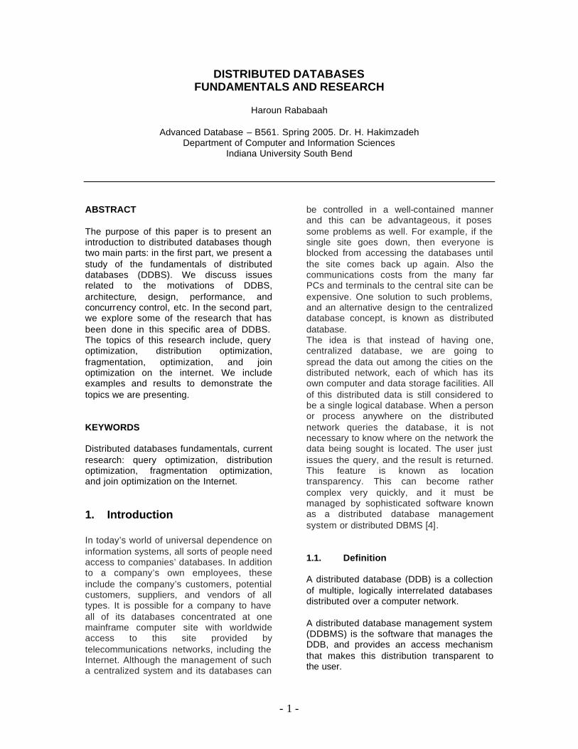
of replicated data across the network. 2. DDBS Architecture 2.1. The Hardware Due to the extended functionality the DDBS must be capable of, the DDBS design becomes more complex and more sophisticated. At the physical level the differences between centralized and distributed systems are: § Multiple computers called sites. § These sites are connected via a

communication network, to enable the data/query communications. Figure 1.1 illustrates this architecture.

Figure 2.1. Client/server architecture [1]

sever

client

Site 4

client

Site 1

client

Site 2

server

Site 3

Communication network

- 3 -

Networks can have several types of topologies that defines how nodes are physically and logically connected. One of the popular topologies used in DDBS, the client-server architecture is described as follows: the principle idea of this architecture is to define specialized servers with specific functionalities such as: printer server, mail server, file server, etc. these serves then are connected to a network of clients that can access the services of these servers. Stations (servers or clients) can have different design complexities starting from diskless client to combined server-client machine. This is illustrated in Figure 1.1.

The server-client architecture requires some kind of function definition for servers and clients. Th e DBMS functions are divided between servers and clients using different approaches. We present a common approach that is used with relational DDBS, called centralized DMBS at the server level. The client refers to a data distribution dictionary to know how to decompose the global query in to multiple local queries. The interaction is done as follows: 1. Client parses the user’s query and

decomposes it into independent site queries.

2. Client forwards each independent query to the corresponding server by consulting with the data distribution dictionary.

3. Each server process the local query, and sends back the resulting relation to the client.

4. Client combines (manually by the user, or automatically by client abstract) the received subqueries, and do more processing if needed to get to the final target result.

We would like to discuss the different architectures of DDBS for the two main types, the client/server, and the distributed databases [4]: The client/server: The file server approach: the simplest tactic is known as the file server approach. When a client computer on the LAN needs to query, update, or otherwise use a file on the server, the entire file must be sent from the server to that client. All of

the querying, updating, or other processing is then performed in the client computer. If changes were made to the file, the entire file is then shipped back to the server. Clearly, for files of even moderate size, shipping entire files back and forth across the LAN with any frequency will be very costly. In terms of concurrency control, obviously the entire file must be locked while one of the clients is updating even one record in it. Other than providing a basic file-sharing capability, this arrangement’s drawbacks render it not very practical or useful. DBMS server approach: A much better arrangement is variously known as the database server or DBMS server approach. Again, the database is located at the server, but this time, the processing is split between the client and the server, and there is much less data traffic on the network. Say that someone at a client computer wants to query the database at the server. The query is entered at the client, and the client computer performs the initial keyboard and screen interaction processing, as well as initial syntax checking of the query. The system then ships the query over the LAN to the server where the query is actually run against the database. Only the results are shipped back to the client. Certainly, this is a much better arrangement than the file server approach! The network data traffic is reduced to a tolerable level, even for frequently queried databases. Also, security and concurrency control can be handled at the server in a much more contained way. The only real drawback to this approach is that the company must invest in a sufficiently powerful server to keep up with all of the activity concentrated there.

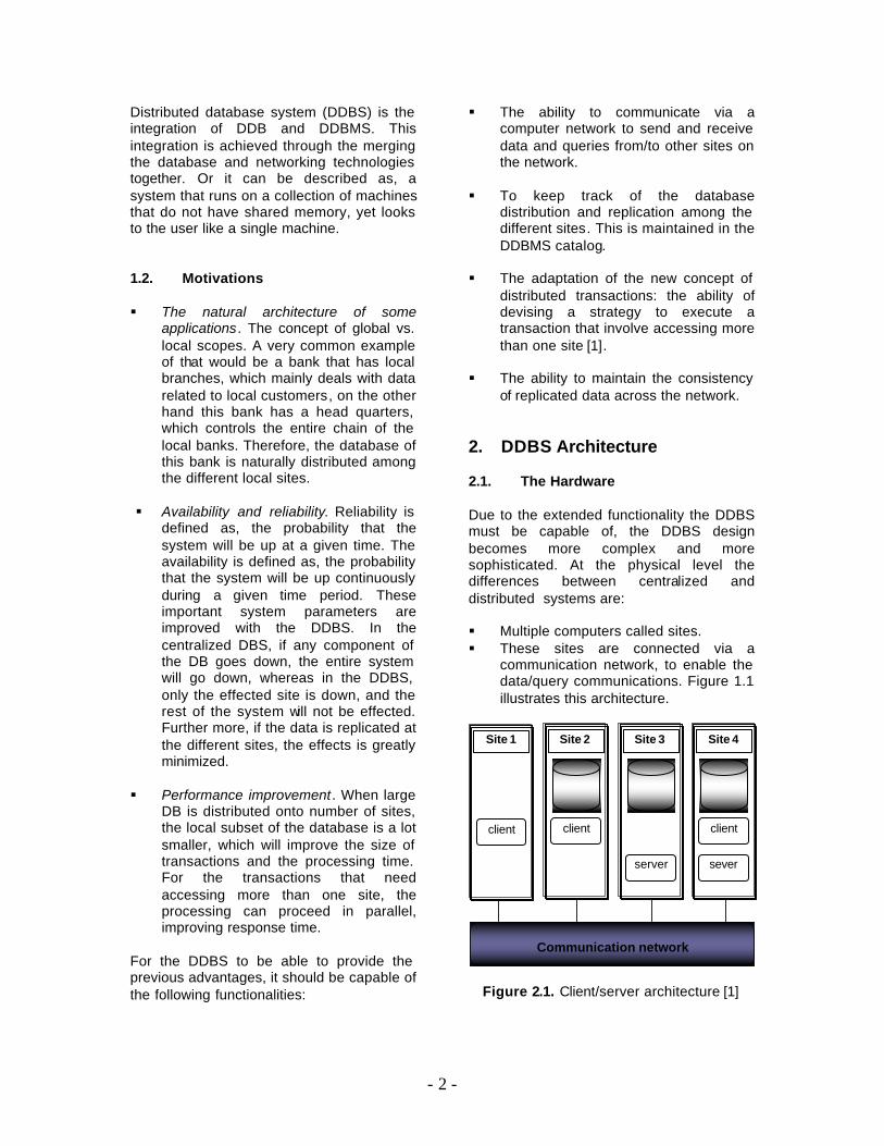
Two-tier client/server: Another issue involving the data on a LAN is the fact that some databases can be stored on a client PC’s own hard drive while other databases that the client might access are stored on the LAN’s server. This is also known as a two-tier approach, (Figure 1.2). Software has been developed that makes the location of the data transparent to the user at the client. In this mode of operation, the user issues a query at the client, and the software first checks to see if the required data is on the PC’s own hard drive. If it is, the data is

- 4 -

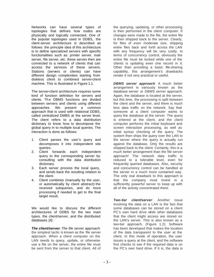
retrieved from it, and that is the end of the story. If it is not there, then the software automatically looks for it on the server. In an even more sophisticated three-tier approach (Figure 1.3), if the software doesn’t find the data on the client PC’s hard drive or on the LAN server, it can leave the LAN through a gateway computer and look for the data on, for example, a large, mainframe computer that may be reachable from many LANs.

Figure 2.2. Two-tier client/server [4]

Figure 2.3. Three-tier client/server [4] Three-tier approach: In another use of the term three-tier approach, the three tiers are the client PCs, servers known as application servers, and other servers known as database servers, (Figure 1.4). In this arrangement, local screen and keyboard interaction is still handled by the clients, but they can now request a variety of applications to be performed at and by the

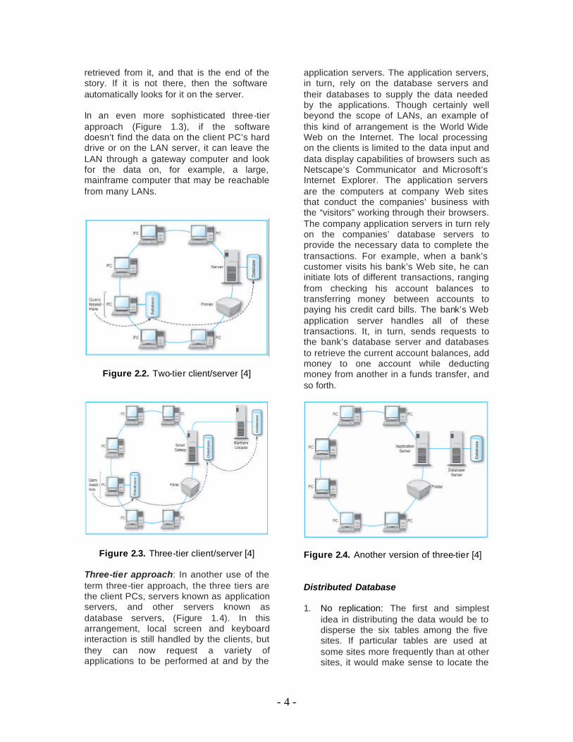
application servers. The application servers, in turn, rely on the database servers and their databases to supply the data needed by the applications. Though certainly well beyond the scope of LANs, an example of this kind of arrangement is the World Wide Web on the Internet. The local processing on the clients is limited to the data input and data display capabilities of browsers such as Netscape’s Communicator and Microsoft’s Internet Explorer. The application servers are the computers at company Web sites that conduct the companies’ business with the “visitors” working through their browsers. The company application servers in turn rely on the companies’ database servers to provide the necessary data to complete the transactions. For example, when a bank’s customer visits his bank’s Web site, he can initiate lots of different transactions, ranging from checking his account balances to transferring money between accounts to paying his credit card bills. The bank’s Web application server handles all of these transactions. It, in turn, sends requests to the bank’s database server and databases to retrieve the current account balances, add money to one account while deducting money from another in a funds transfer, and so forth.

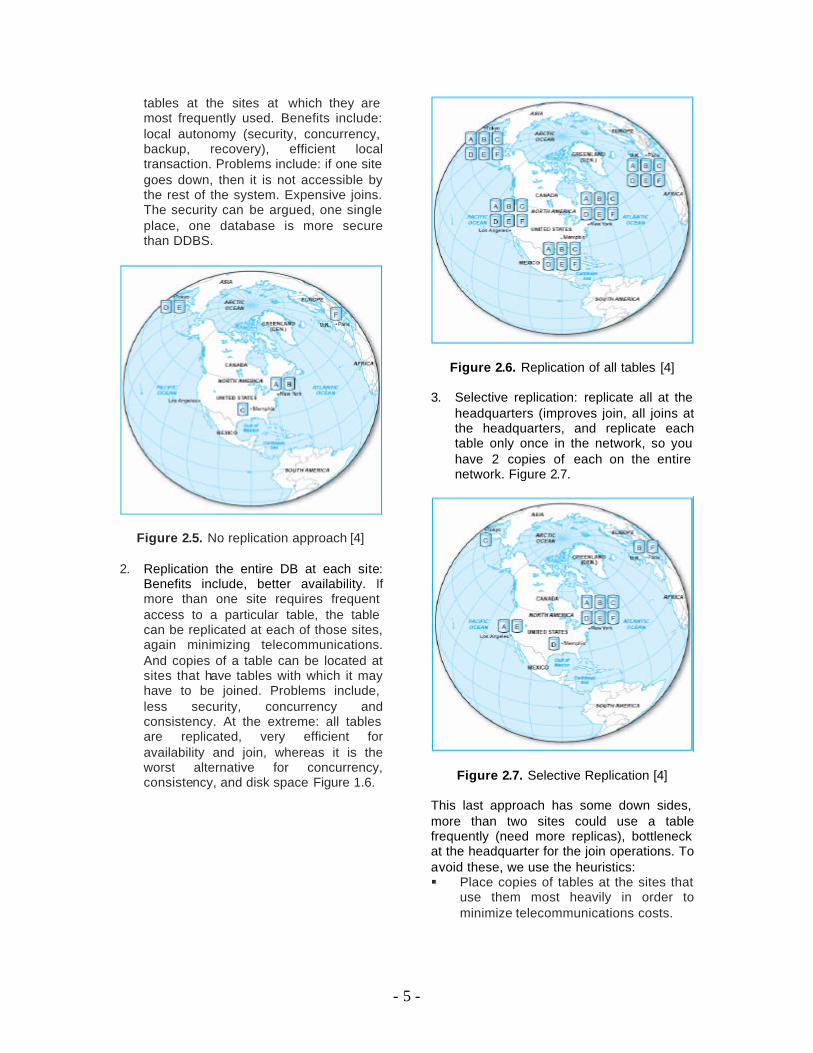
Figure 2.4. Another version of three-tier [4] Distributed Database 1. No replication: The first and simplest

idea in distributing the data would be to disperse the six tables among the five sites. If particular tables are used at some sites more frequently than at other sites, it would make sense to locate the

- 5 -

tables at the sites at which they are most frequently used. Benefits include: local autonomy (security, concurrency, backup, recovery), efficient local transaction. Problems include: if one site goes down, then it is not accessible by the rest of the system. Expensive joins. The security can be argued, one single place, one database is more secure than DDBS.

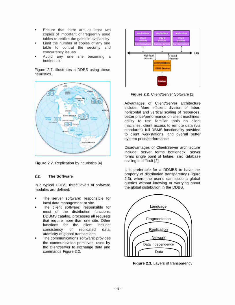
Figure 2.5. No replication approach [4] 2. Replication the entire DB at each site:

Benefits include, better availability. If more than one site requires frequent access to a particular table, the table can be replicated at each of those sites, again minimizing telecommunications. And copies of a table can be located at sites that have tables with which it may have to be joined. Problems include, less security, concurrency and consistency. At the extreme: all tables are replicated, very efficient for availability and join, whereas it is the worst alternative for concurrency, consistency, and disk space Figure 1.6.

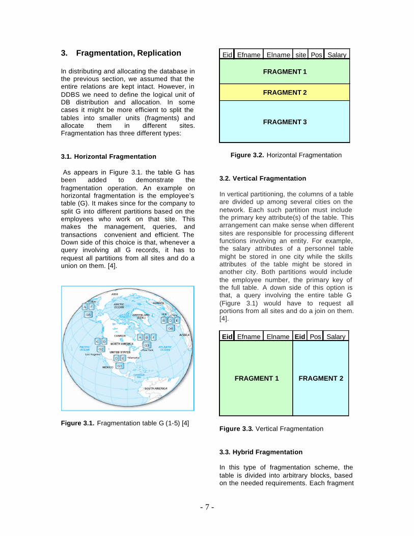
Figure 2.6. Replication of all tables [4] 3. Selective replication: replicate all at the

headquarters (improves join, all joins at the headquarters, and replicate each table only once in the network, so you have 2 copies of each on the entire network. Figure 2.7.

Figure 2.7. Selective Replication [4] This last approach has some down sides, more than two sites could use a table frequently (need more replicas), bottleneck at the headquarter for the join operations. To avoid these, we use the heuristics: § Place copies of tables at the sites that

use them most heavily in order to minimize telecommunications costs.

- 6 -

§ Ensure that there are at least two copies of important or frequently used tables to realize the gains in availability.

§ Limit the number of copies of any one table to control the security and concurrency issues.

§ Avoid any one site becoming a bottleneck.

Figure 2.7. illustrates a DDBS using these heuristics.

Figure 2.7. Replication by heuristics [4] 2.2. The Software In a typical DDBS, three levels of software modules are defined: § The server software: responsible for

local data management at site. § The client software: responsible for

most of the distribution functions; DDBMS catalog, processes all requests that require more than one site. Other functions for the client include: consistency of replicated data, atomicity of global transactions.

§ The communications software: provides the communication primitives, used by the client/server to exchange data and commands Figure 2.2.

Figure 2.2. Client/Server Software [2]

Advantages of Client/Server architecture include: More efficient division of labor, horizontal and vertical scaling of resources, better price/performance on client machines, ability to use familiar tools on client machines, client access to remote data (via standards), full DBMS functionality provided to client workstations, and overall better system price/performance Disadvantages of Client/Server architecture include: server forms bottleneck, server forms single point of failure, and database scaling is difficult [2]. It is preferable for a DDMBS to have the property of distribution transparency (Figure 2.3), where the user’s can issue a global queries without knowing or worrying about the global distribution in the DDBS.

Figure 2.3. Layers of transparency

Network

Replication

Fragmentation

Language

Data

Data Independence

- 7 -

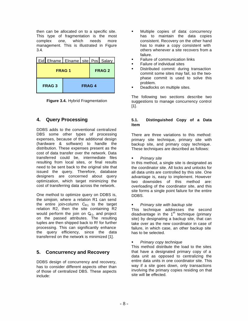
3. Fragmentation, Replication In distributing and allocating the database in the previous section, we assumed that the entire relations are kept intact. However, in DDBS we need to define the logical unit of DB distribution and allocation. In some cases it might be more efficient to split the tables into smaller units (fragments) and allocate them in different sites. Fragmentation has three different types: 3.1. Horizontal Fragmentation As appears in Figure 3.1. the table G has been added to demonstrate the fragmentation operation. An example on horizontal fragmentation is the employee’s table (G). It makes since for the company to split G into different partitions based on the employees who work on that site. This makes the management, queries, and transactions convenient and efficient. The Down side of this choice is that, whenever a query involving all G records, it has to request all partitions from all sites and do a union on them. [4].

Figure 3.1. Fragmentation table G (1-5) [4]

Eid Efname Elname site Pos Salary

FRAGMENT 1

FRAGMENT 2

FRAGMENT 3

Figure 3.2. Horizontal Fragmentation 3.2. Vertical Fragmentation In vertical partitioning, the columns of a table are divided up among several cities on the network. Each such partition must include the primary key attribute(s) of the table. This arrangement can make sense when different sites are responsible for processing different functions involving an entity. For example, the salary attributes of a personnel table might be stored in one city while the skills attributes of the table might be stored in another city. Both partitions would include the employee number, the primary key of the full table. A down side of this option is that, a query involving the entire table G (Figure 3.1) would have to request all portions from all sites and do a join on them. [4].

Eid Efname Elname Eid Pos Salary

FRAGMENT 1 FRAGMENT 2

Figure 3.3. Vertical Fragmentation 3.3. Hybrid Fragmentation In this type of fragmentation scheme, the table is divided into arbitrary blocks, based on the needed requirements. Each fragment

- 8 -

then can be allocated on to a specific site. This type of fragmentation is the most complex one, which needs more management. This is illustrated in Figure 3.4.

Eid Efname Elname site Pos Salary

FRAG 1 FRAG 2

FRAG 3 FRAG 4

Figure 3.4. Hybrid Fragmentation 4. Query Processing DDBS adds to the conventional centralized DBS some other types of processing expenses, because of the additional design (hardware & software) to handle the distribution. These expenses present as the cost of data transfer over the network. Data transferred could be, intermediate files resulting from local sites, or final results need to be sent back to the original site that issued the query. Therefore, database designers are concerned about query optimization, which target minimizing the cost of transferring data across the network. One method to optimize query on DDBS is, the simijoin, where a relation R1 can send the entire join-column CR1 to the target relation R2, then the site containing R2 would perform the join on CR1, and project on the passed attributes. The resulting tuples are then shipped back to R! for further processing. This can significantly enhance the query efficiency, since the data transferred on the network is minimized [1]. 5. Concurrency and Recovery DDBS design of concurrency and recovery, has to consider different aspects other than of those of centralized DBS. These aspects include:

§ Multiple copies of data: concurrency has to maintain the data copies consistent. Recovery on the other hand has to make a copy consistent with others whenever a site recovers from a failure.

§ Failure of communication links § Failure of individual sites § Distributed commit: during transaction

commit some sites may fail, so the two-phase commit is used to solve this problem.

§ Deadlocks on multiple sites. The following two sections describe two suggestions to manage concurrency control [1]. 5.1. Distinguished Copy of a Data Item There are three variations to this method: primary site technique, primary site with backup site, and primary copy technique. These techniques are described as follows: § Primary site In this method, a single site is designated as the coordinator site. All locks and unlocks for all data units are controlled by this site. One advantage is, easy to implement. However two downsides of this method are: overloading of the coordinator site, and this site forms a single point failure for the entire DDBS. § Primary site with backup site This technique addresses the second disadvantage in the 1st technique (primary site) by designating a backup site, that can take over as the new coordinator in case of failure, in which case, an other backup site has to be selected. § Primary copy technique This method distribute the load to the sites that have a designated primary copy of a data unit as opposed to centralizing the entire data units in one coordinator site. This way if a site goes down, only transactions involving the primary copies residing on that site will be effected.

- 9 -

5.2. Voting This method does not designate any distinguished copy or site to be the coordinator as suggested in the 1st two methods described above. When a site attempts to lock a data unit, requests to all sites having the desired copy, must be sent asking to lock this copy. If the requesting transaction did was not granted the lock by the majority voting from the sites, then the transaction fails and sends cancellation to all. Otherwise it keeps the lock and informs all sites that it has been granted the lock. 5.3. Recovery The first step of dealing with the recovery problem is to identify that there was a failure, what type was it, and at which site did that happen. Dealing with distributed recovery requires aspects include: database logs, and update protocols, transaction failure recovery protocol, etc [1]. 6. Research in DDBS In this section, we present some of the current research being done in DDBS, specifically, distributed query optimization, 6.1. Distributed Query Processing

Using Active Networks. [5] This paper, presented an efficient method for Implementing query processing on high-speed active WANs. The paper studied the traditional criteria for distributed query optimization, and devised a new criteria for approaching DDBS query optimization, based on the different characteristics of low and high speed networks. Conventional vs. high-speed networks In conventional networks, transmission delay is regarded as the dominant factor in the communication cost function. For that reason, many distributed query processing algorithms are devised to minimize the amount of data transmitted over the network. However, in high speed networks,

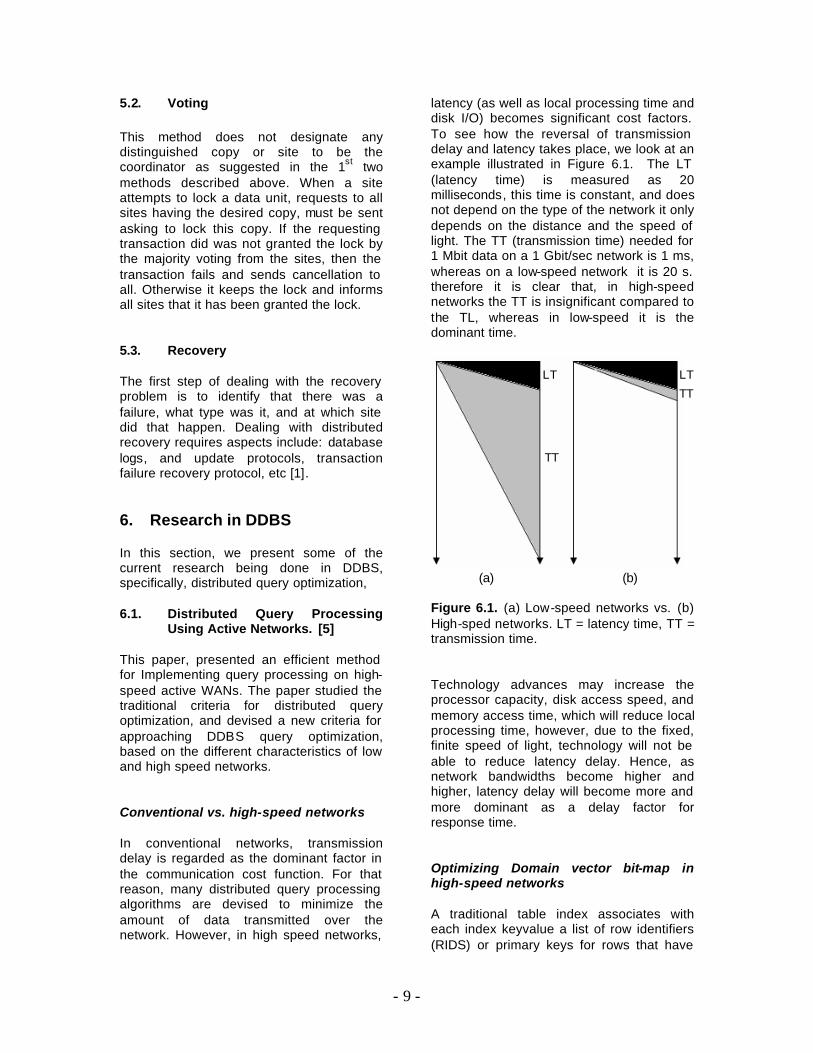
latency (as well as local processing time and disk I/O) becomes significant cost factors. To see how the reversal of transmission delay and latency takes place, we look at an example illustrated in Figure 6.1. The LT (latency time) is measured as 20 milliseconds, this time is constant, and does not depend on the type of the network it only depends on the distance and the speed of light. The TT (transmission time) needed for 1 Mbit data on a 1 Gbit/sec network is 1 ms, whereas on a low-speed network it is 20 s. therefore it is clear that, in high-speed networks the TT is insignificant compared to the TL, whereas in low-speed it is the dominant time.

(a) (b)

Figure 6.1. (a) Low-speed networks vs. (b) High-sped networks. LT = latency time, TT = transmission time. Technology advances may increase the processor capacity, disk access speed, and memory access time, which will reduce local processing time, however, due to the fixed, finite speed of light, technology will not be able to reduce latency delay. Hence, as network bandwidths become higher and higher, latency delay will become more and more dominant as a delay factor for response time. Optimizing Domain vector bit-map in high-speed networks A traditional table index associates with each index keyvalue a list of row identifiers (RIDS) or primary keys for rows that have

LT LT

TT

TT

- 10 -

that value. It is well known that the list of rows associated with a given index keyvalue can be represented by a bitmap or bit vector. In a bitmap representation, each row in a table is associated with a bit in a long string, an N-bit string if there are N rows in the table, and the bit is set to 1 in the bitmap if the associated row is contained in the list represented; otherwise the bit is set to 0. This technique is particularly attractive when the set of possible keyvalues in the index is small, with a large number of rows, e.g. an index on a sex attribute, where sex = ‘Male’ or sex = ‘Female’. In this example, there will be only two lists to be represented in an index, and the total number of bits stored will be 2N, while one out of two bits will (usually) be 1 in both bitmaps. (We can’t be sure that these bitmaps will be complements of each other, since a deleted row will result in a bit that is zero in both.) When a large number of values exist in an index, each of the bitmaps is likely to be rather sparse, that is, very few bits will be 1 in the bitmaps, resulting in heavy storage requirements for storing a lot of zeros. In such cases, bitmap compression is used. The point of using bitmap indices, of course, is the tremendous performance advantage to be gained. To start with there is reduced I/O when a large fraction of a large table is represented using a bitmap rather than by a RID list. In addition, a bitmap for a foundset on 10 million rows will require a maximum of only slightly more than a megabyte of storage (10 million bits = 1.25 million bytes) so bitmaps can commonly be pipelined or cached in memory, and the RIDS represented are automatically held in RID order, useful when combining predicates and when retrieving rows from disk. In addition, the most common operations used to combine predicates, AND and OR, can be performed using very efficient instructions that gain a lot of parallelism by executing 32 or 64 bits in parallel on most modern processors. This discussion is taken from [6]. In this paper a new efficient algorithm was devised for executing distributed queries. The criteria was to minimize not only the amount of transferred data, but number of messages on the network (the latency) as

described earlier. They gave the following example, which illustrates their algorithm: DVA = Domain Vector Acceleration. JV = join vector formed by ANDing both DVs of the two relations. DVI = domain vector identifier. Consider a query Q requiring a join among relation R1 at site S1, R2 at site S2, …, and Rn at site Sn on a common attribute A, where site S1 initiates the join. Q = R1 |X| R2 |X|… |X| Rn 1. At site S1 , retrieve DV (R1.A) from disk

and simultaneously setup a point-to-multipoint unidirectional connection from site S1 to site Si (i = 2,..., n)

2. Send Q together with DV (R1.A) to site Si (i = 2,..., n), then tear down this connection

3. At each Si (i=2,...,n), retrieve DV(Ri.A), simultaneously setup a point-to-multipoint unidirectional connection from site Si to every other site Sj (j = 1,..,i-1, i+1,...,n)

4. From each Si (i=2,...,n) ship its DV(Ri.A) to every other site Sj (j = 1,...,i-1, i+1,...,n)

5. At each site Si (i = 1,..,n), logically AND DV(Ri.A) (i = 1,...,n) to create JV

6. At each Si (i=1,...,n), use DVI(Ri.A) to read participating tuples, Ri.A’, in JV order.

7. From each site Si (i = 2,...,n) ship Ri.A’ to site R1 along the same connection set up used in step c, then tear down each connection

8. At S1, merge join Ri .A’ (i=1,...,n) (already sorted in JV order) to get the final result.

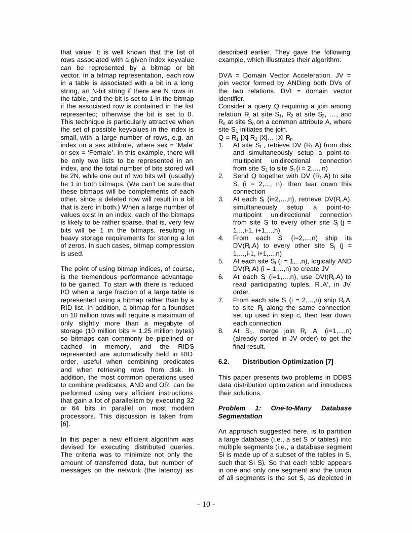
6.2. Distribution Optimization [7] This paper presents two problems in DDBS data distribution optimization and introduces their solutions. Problem 1: One-to-Many Database Segmentation An approach suggested here, is to partition a large database (i.e., a set S of tables) into multiple segments (i.e., a database segment Si is made up of a subset of the tables in S, such that Si S). So that each table appears in one and only one segment and the union of all segments is the set S, as depicted in

- 11 -

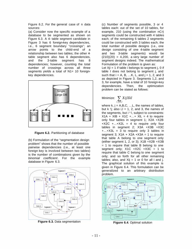
Figure 6.2. For the general case of n data sources: (a) Consider now the specific example of a database to be segmented as shown on Figure 6.3. A 4- table segment candidate in Figure 3 has 6 foreign-key dependencies, i.e., 6 segment boundary “crossings”; an arrow points to the child-end of a relationship between two tables; the other 4-table segment also has 6 dependencies, and the 3-table segment has 8 dependencies; however, counting the total number of crossings across all three segments yields a total of N1= 10 foreign-key dependencies.

Figure 6.2. Partitioning of database (b) Formulation of the “segmentation design problem” shows that the number of possible pairwise dependencies (i.e., at least one foreign key is involved between two tables) is the number of combinations given by the binomial coefficient . For the example database in Figure 6.3.

Figure 6.3. Data segmentation

(c) Number of segments possible, 3 or 4 tables each: out of the set of 10 tables, for example, 210 (using the combination nCr) segments could be constructed with 4 tables each; of the remaining 6 tables 2 segments could be constructed with 3 tables each; the total number of possible designs (i.e., one design consisting of one 4-table segment and two 3-table segments) would be (210)(20) = 4,200, a very large number of segment designs indeed. The mathematical Formulation of the problem is given as: Let Xji = 1 if table i belongs to segment j, 0 if table I does not belong to segment j, and such that i = A, B, …K, L, and j = 1, 2, and 3 as depicted in Figure 3. Segments 1,2, and 3, for example, have a total of 10 foreign-key dependencies. Then, the optimization problem can be stated as follows:

Minimize: ∑lkji

XijXkl,,,

where k, j = A,B,C, …L, the names of tables, but k ¹j; also i,l = 1, 2, and 3, the names of the segments, but i ¹ l, subject to constraints: X1A + XIB + X1C +…+ XlL = 4 to require only four tables in segment 1; X2A +X2B +X2C +…+X2L = 4 to require only four tables in segment 2; X3A +X3B +X3C +…+X3L = 3 to require only 3 tables in segment 3; X1A + X2A +X3A = 1 to require that table A belong to one segment only (either segment 1, 2, or 3); X1B +X2B +X3B = 1 to require that table B belong to one segment only; X1C +X2C +X3C = 1 to require that table C belong to one segment only; and so forth for all other remaining tables; also, and Xij = 1 or 0 for all i and j. The graphical solution of this example is given in Figure 6.4. This formulation can be generalized to an arbitrary distribution problem.

Figure 6.4. Optimal solution

Single Large DB

DB1 DB2 DBn

- 12 -

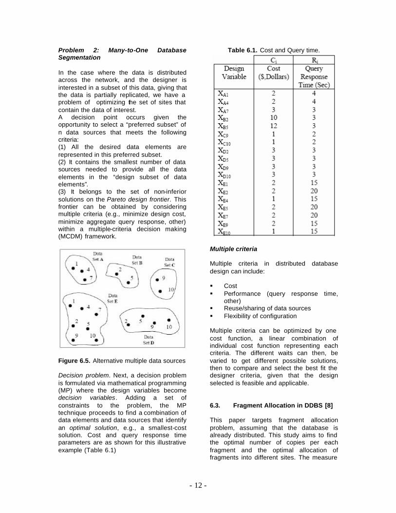
Problem 2: Many-to-One Database Segmentation In the case where the data is distributed across the network, and the designer is interested in a subset of this data, giving that the data is partially replicated, we have a problem of optimizing the set of sites that contain the data of interest. A decision point occurs given the opportunity to select a “preferred subset” of n data sources that meets the following criteria: (1) All the desired data elements are represented in this preferred subset. (2) It contains the smallest number of data sources needed to provide all the data elements in the “design subset of data elements”. (3) It belongs to the set of non-inferior solutions on the Pareto design frontier. This frontier can be obtained by considering multiple criteria (e.g., minimize design cost, minimize aggregate query response, other) within a multiple-criteria decision making (MCDM) framework.

Figure 6.5. Alternative multiple data sources

Decision problem. Next, a decision problem is formulated via mathematical programming (MP) where the design variables become decision variables. Adding a set of constraints to the problem, the MP technique proceeds to find a combination of data elements and data sources that identify an optimal solution, e.g., a smallest-cost solution. Cost and query response time parameters are as shown for this illustrative example (Table 6.1)

Table 6.1. Cost and Query time.

Multiple criteria Multiple criteria in distributed database design can include: § Cost § Performance (query response time,

other) § Reuse/sharing of data sources § Flexibility of configuration Multiple criteria can be optimized by one cost function, a linear combination of individual cost function representing each criteria. The different waits can then, be varied to get different possible solutions, then to compare and select the best fit the designer criteria, given that the design selected is feasible and applicable. 6.3. Fragment Allocation in DDBS [8] This paper targets fragment allocation problem, assuming that the database is already distributed. This study aims to find the optimal number of copies per each fragment and the optimal allocation of fragments into different sites. The measure

- 13 -

of optimality are: Assume that we have a WAN consisting of sites S = {S1, S2, …, Sm}, on which a set of transactions T = {T1, T2, …, Tq} is running, and a set of fragments F = {F1, F2, …, Fn} 1. Minimal cost: The cost function consists

of the cost of storing each Fj on site Sk, the cost of querying Fj at site Sk, the cost of updating Fj at all sites where it is stored, and the cost of data communication.

2. Performance: Two well-known strategies are to minimize the response time and to maximize the system throughput at each site.

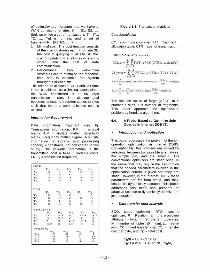
The criteria of allocation: CPU and I/O time is not considered as a limiting factor, since the WAN considered is at 50 kbps transmission rate. The ultimate goal becomes, allocating fragment copies to sites such that the total communication cost is minimal. Information Requirement Data information: fragment size Fj. Transaction information: RM = retrieval matrix, UM = update matrix, Selectivity matrix, Frequency matrix, Figure 6.6. Site information is storage and processing capacity = constrains (not considered in this study). The network information, is the transmitting cost = fixed + variable costs. FREQ = transaction frequency,

Figure 6.6. Transaction matrices Cost formulation CC = communication cost, FAT = fragment allocation table, CTR = cost of transmission,

The solution space of large (2m-1)n, m = number o sites, n = number of fragments. This paper approach the optimization problem by heuristic algorithms. 6.4. A Probe-Based to Optimize Join

Queries in Internet DDB [9]. § Introduction and motivation This paper addresses the problem of the join operation optimization in Internet DDBS. Conventionally, this problem was solved by selecting between two possible alternatives: the simple join, and the smi-join. The conventional optimizers are static ones, in the sense that they rely on the assumption that the needed parameters involved in the optimization criteria is given and they are static. However, in the Internet DDBS, these parameters are far from static, and they should be dynamically updated. This paper addresses this need and presents an adaptive solution to dynamically optimize the join operation. § Data transfer cost analysis SQO: static optimizer, RTO: runtime optimizer, R = Relation, a = the projection attribute, l = local, r = remote, S = tuple size, N = number of tuples, j0 = joint, j1 = semi-joint, C0 = fixed transfer cost, C1 = transfer cost per byte, and C() = total cost.

C(j0) = C0 + C1.Sr.Nr C(j1) = 2C0 + C1(Sla.Nl + S(j0r)

- 14 -

SQO will be in accurate in comparing between the two costs C(j0) and C(j1) because the following parameters are not static: C1 depends on the instantaneous situation of the internet, and never fixed. The estimation of the intermediate result S(j0r) is not accurate because it the uses the relation: S(j0r) = domain(a) . selectivity(Rl,a) . slectivi ty(Rr, a) The assumptions are, Sa is fixed, and tuples are distributed between Rl, Rr independent of a. § The RTO algorithm 1. Estimate the term C1.Sj0r: send x tuples

(these tupls consists only of the ‘a’ attribute) to site 2 and join this x subset with the Rr at site 2. measure the response time and normalize it to x.

2. Estimate the term C1.Sr: site 1 receives x tuples of Rr, join with Rl, estimate the execution time and normalize to x.

3. The final comparison of the two alternatives will be:

C(j0) = Nl.Cl2r + estimated(Sj0r).Cr2l C(j1) = Nr.Cr2l

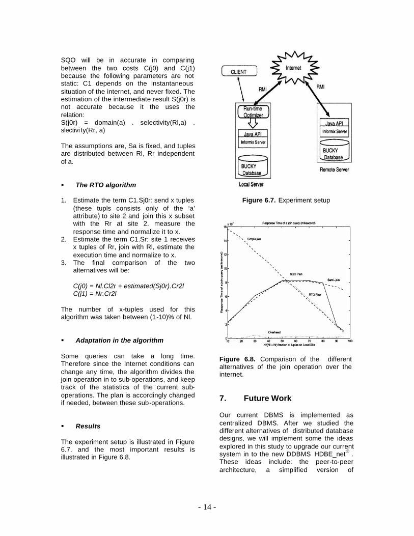
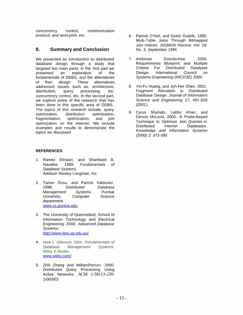
The number of x-tuples used for this algorithm was taken between (1-10)% of Nl. § Adaptation in the algorithm Some queries can take a long time. Therefore since the Internet conditions can change any time, the algorithm divides the join operation in to sub-operations, and keep track of the statistics of the current sub-operations. The plan is accordingly changed if needed, between these sub-operations. § Results The experiment setup is illustrated in Figure 6.7. and the most important results is illustrated in Figure 6.8.

Figure 6.7. Experiment setup

Figure 6.8. Comparison of the different alternatives of the join operation over the internet. 7. Future Work Our current DBMS is implemented as centralized DBMS. After we studied the different alternatives of distributed database designs, we will implement some the ideas explored in this study to upgrade our current system in to the new DDBMS HDBE_net® . These ideas include: the peer-to-peer architecture, a simplified version of

- 15 -

concurrency control, communication protocol, and semi-joint, etc. 8. Summary and Conclusion We presented an introduction to distributed database design through a study that targeted two main parts: in the first part we presented an exploration of the fundamentals of DDBS, and the alternatives of their design. These alternatives addressed issues such as, architecture, distribution, query processing, etc. concurrency control, etc. In the second part, we explore some of the research that has been done in this specific area of DDBS. The topics of this research include, query optimization, distribution optimization, fragmentation, optimization, and join optimization on the internet. We include examples and results to demonstrate the topics we discussed. REFERENCES 1. Ramez Elmasri, and Shamkant B.

Navathe. 1999. Fundamentals of Database Systems. Addison Wesley Longman, Inc.

2. Tamer Özsu, and Patrick Valduriez. 1998. Distributed Database Management Systems. Purdue University, Computer Science department. www.cs.purdue.edu

3. The University of Queensland, School of Information Technology and Electrical Engineering. 2000. Advanced Database Systems. http://www.itee.uq.edu.au/

4. Mark L. Gillenson. 2004. Fundamentals of Database Management Systems. Wiley E-Books. www.wiley.com/

5. Zhili Zhang and WiliamPerrizo. 2000. Distributed Query Processing Using Active Networks. ACM 1-58113-239-5/00/003

6. Patrick O’Neil, and Goetz Graefe. 1995.

Multi-Table Joins Through Bitmapped Join Indices. SIGMOD Record, Vol. 24, No. 3, September 1995

7. Ambrose Goicoechea. 2000.

Requirements Blueprint and Multiple Criteria For Distributed Database Design. International Council on Systems Engineering (INCOSE) 2000.

8. Yin-Fu Huang, and Jyh-Her Chen. 2001.

Fragment Allocation in Distributed Database Design. Journal of Information Science and Engineering 17, 491-506 (2001).

9. Cyrus Shahabi, Latifur Khan, and Dennis McLeod. 2000. A Probe-Based Technique to Optimize Join Queries in Distributed Internet Databases. Knowledge and Information Systems (2000) 2: 373-385