1

Distributed Deadlock

91.515

2

DS Deadlock Topics • Prevention

– Too expensive in time and network traffic in a distributed system

• Avoidance – Determining safe and unsafe states would

require a huge number of messages in a DS • Detection

– May be practical, and is primary chapter focus • Resolution

– More complex than in non-distributed systems

3

DS Deadlock Detection

• Bi-partite graph strategy modified – Use Wait For Graph (WFG or TWF)

• All nodes are processes (threads) • Resource allocation is done by a process (thread)

sending a request message to another process (thread) which manages the resource (client - server communication model, RPC paradigm)

– A system is deadlocked IFF there is a directed cycle (or knot) in a global WFG

4

DS Deadlock Detection, Cycle vs. Knot

• The AND model of requests requires all resources currently being requested to be granted to un-block a computation – A cycle is sufficient to declare a deadlock with this

model • The OR model of requests allows a computation

making multiple different resource requests to un-block as soon as any are granted – A cycle is a necessary condition – A knot is a sufficient condition

5

P8

P10 P9

P7

P6 P5

P4

P3 P2

P1

S1

S3 S2

Deadlock in the AND model; there is a cycle but no knot

No Deadlock in the OR model

6

P8

P10 P9

P7

P6 P5

P4

P3 P2

P1

S1

S3 S2

Deadlock in both the AND model and the OR model; there are cycles and a knot

7

DS Detection Requirements

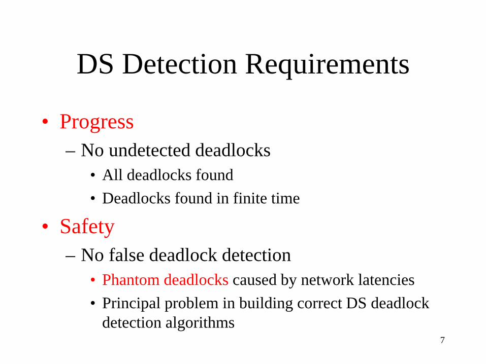
• Progress – No undetected deadlocks

• All deadlocks found • Deadlocks found in finite time

• Safety – No false deadlock detection

• Phantom deadlocks caused by network latencies • Principal problem in building correct DS deadlock

detection algorithms

8

Control Framework • Approaches to DS deadlock detection fall in

three domains: – Centralized control

• one node responsible for building and analyzing a real WFG for cycles

– Distributed Control • each node participates equally in detecting

deadlocks … abstracted WFG

– Hierarchical Control • nodes are organized in a tree which tends to look

like a business organizational chart

9

Total Centralized Control • Simple conceptually:

– Each node reports to the master detection node – The master detection node builds and analyzes

the WFG – The master detection node manages resolution

when a deadlock is detected • Some serious problems:

– Single point of failure – Network congestion issues – False deadlock detection

10

Total Centralized Control (cont)

• The Ho-Ramamoorthy Algorithms – Two phase (can be for AND or OR model)

• each site has a status table of locked and waited resources

• the control site will periodically ask for this table from each node

• the control node will search for cycles and, if found, will request the table again from each node

• Only the information common in both reports will be analyzed for confirmation of a cycle

• The algorithm turns out to detect phantom deadlocks

11

Total Centralized Control (cont)

• The Ho-Ramamoorthy Algorithms (cont) – One phase (can be for AND or OR model)

• each site keeps 2 tables; process status and resource status

• the control site will periodically ask for these tables (both together in a single message) from each node

• the control site will then build and analyze the WFG, looking for cycles and resolving them when found

• So far, algorithm seems to be phantom free

12

Distributed Control

• Each node has the same responsibility for, and will expend the same amount of effort in detecting deadlock – The WFG becomes an abstraction, with any

single node knowing just some small part of it – Generally detection is launched from a site

when some thread at that site has been waiting for a “long” time in a resource request message

13

Distributed Control Models • Four common models are used in building

distributed deadlock control algorithms: – Path-pushing

• path info sent from waiting node to blocking node – Edge-chasing

• probe messages are sent along graph edges – Diffusion computation

• echo messages are sent along graph edges

– Global state detection • sweep-out, sweep-in (weighted echo messages);

WFG construction and reduction

14

Path-pushing • Obermarck’s algorithm for path propagation

is described in the text: (an AND model) – based on a database model using transaction processing – sites which detect a cycle in their partial WFG views

convey the paths discovered to members of the (totally ordered) transaction

– the highest priority transaction detects the deadlock “Ex => T1 => T2 => Ex”

– Algorithm can detect phantoms due to its asynchronous snapshot method

15

Edge Chasing Algorithms

• Chandy-Misra-Haas Algorithm (an AND model) – probe messages M(i, j, k)

• initiated by Pj for Pi and sent to Pk • probe messages work their way through the WFG

and if they return to sender, a deadlock is detected • make sure you can follow the example in Figure 7.1

of the book

16

Chandy-Misra-Haas Algorithm

P8

P10 P9

P7

P6 P5

P4

P3 P2

P1 Probe (1, 3, 4)

Probe (1, 7, 10)

Probe (1, 6, 8)

Probe (1, 9, 1) S1

S3 S2

P1 launches

17

Edge Chasing Algorithms (cont) • Mitchell-Meritt Algorithm (an AND model)

– propagates message in the reverse direction – uses public - private labeling of messages – messages may replace their labels at each site – when a message arrives at a site with a

matching public label, a deadlock is detected (by only the process with the largest public label in the cycle) which normally does resolution by self - destruct

18

P8

P10 P9

P7

P6 P5

P4

P3 P2

P1

S1

S3 S2

Public 1=> 3 Private 1

Public 3 Private 3

Public 2 => 3 Private 2

1. P6 initially asks P8 for its Public label and changes its own 2 to 3 2. P3 asks P4 and changes its Public label 1 to 3 3. P9 asks P1 and finds its own Public label 3 and thus detects the deadlock P1=>P2=>P3=>P4=>P5=>P6=>P8=>P9=>P1

2

1

3

Mitchell-Meritt Algorithm

19

Deadlock Detection Algorithm

• Mitchell & Merritt’s algorithm [1984] – Detects local and global deadlocks

– Exactly one process detects deadlock

• Simplifies deadlock resolution

– Pair of labels (numbers) used for deadlock detection

– Deadlock detected when a label makes a “round-trip” among set of blocked processes

20

Mitchell-Merritt Example

1,1

1,1

1,3

1,3

1,2

1,2

1,4

1,4

2,1

2,1

3,3

3,3

4,2

4,2

1,4

1,4

Initial State

Blocking Step

Public (count, pid)

Private (count, pid)

BUSY Write to B

BUSY

BUSY

A B

D C

Read from C

Read from A

Arrows indicate waiting. Artificial deadlock without feedback.

BUSY

A B

D C

21

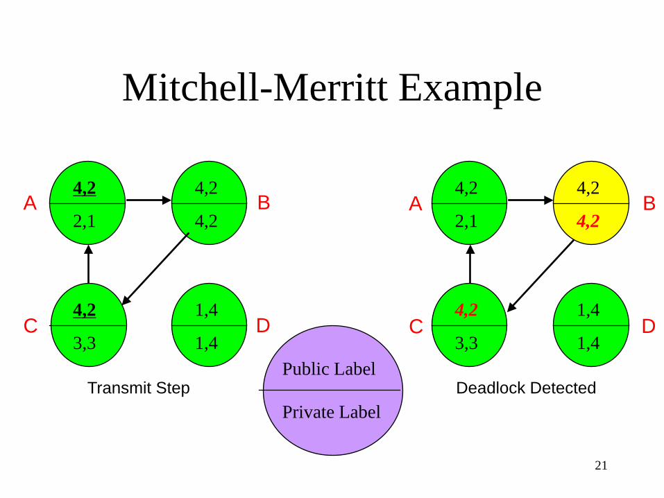
Mitchell-Merritt Example

Public Label

Private Label Transmit Step

4,2

2,1

4,2

3,3

4,2

4,2

1,4

1,4

Deadlock Detected

4,2

2,1

4,2

3,3

4,2

4,2

1,4

1,4

A B

D C

A B

D C

22

Diffusion Computation • Deadlock detection computations are

diffused through the WFG of the system – Query messages are sent from a computation (process

or thread) on a node and diffused across the edges of the WFG

– When a query reaches an active (non-blocked) computation the query is discarded, but when a query reaches a blocked computation the query is echoed back to the originator when (and if) all outstanding queries of the blocked computation are returned to it

– If all queries sent are echoed back to an initiator, there is deadlock

23

Diffusion Computation of Chandy et al (an OR model)

• A waiting computation on node x periodically sends a query to all computations it is waiting for (the dependent set), marked with the originator ID and target ID

• Each of these computations in turn will query their dependent set members (only if they are blocked themselves) marking each query with the originator ID, their own ID and a new target ID they are waiting on

• A computation cannot echo a reply to its requestor until it has received replies from its entire dependent set, at which time it sends a reply marked with the originator ID, its own ID and the dependent (target) ID

• When (and if) the original requestor receives echo replies from all members of its dependent set, it can declare a deadlock when an echo reply’s originator ID and target ID are its own

24

P8

P10 P9

P7

P6 P5

P4

P3 P2

P1

S1

S3 S2

Diffusion Computation of Chandy et al

25

P1 => P2 message at P2 from P1 (P1, P1, P2) P2 => P3 message at P3 from P2 (P1, P2, P3) P3 => P4 message at P4 from P3 (P1, P3, P4) P4 => P5 ETC. P5 => P6 P5 => P7 P6 => P8 P7 => P10 P8 => P9 (P1, P8, P9), now reply (P1, P9, P1) P10 => P9 (P1, P10, P9), now reply (P1, P9, P1) P8 <= P9 reply (P1, P9, P8) P10<= P9 reply (P1, P9, P10) P6 <= P8 reply (P1, P8, P6) P7 <= P10 reply (P1, P10, P7) P5 <= P6 ETC. P5 <= P7 P4 <= P5 P3 <= P4 P2 <= P3 P1 <= P2 reply (P1, P2, P1)

P5 cannot reply until both P6 and P7 replies arrive !

Diffusion Computation of Chandy et al

end condition

deadlock condition

26

Global State Detection

• Based on 2 facts of distributed systems: – A consistent snapshot of a distributed system

can be obtained without freezing the underlying computation

– A consistent snapshot may not represent the system state at any moment in time, but if a stable property holds in the system before the snapshot collection is initiated, this property will still hold in the snapshot

27

Global State Detection (the P-out-of-Q request model)

• The Kshemkalyani-Singhal algorithm is demonstrated in the text – An initiator computation snapshots the system by sending FLOOD

messages along all its outbound edges in an outward sweep – A computation receiving a FLOOD message either returns an

ECHO message (if it has no dependencies itself), or propagates the FLOOD message to it dependencies

• An echo message is analogous to dropping a request edge in a resource allocation graph (RAG)

– As ECHOs arrive in response to FLOODs the region of the WFG the initiator is involved with becomes reduced

– If a dependency does not return an ECHO by termination, such a node represents part (or all) of a deadlock with the initiator

– Termination is achieved by summing weighted ECHO and SHORT messages (returning initial FLOOD weights)

28

Hierarchical Deadlock Detection • These algorithms represent a middle ground

between fully centralized and fully distributed • Sets of nodes are required to report

periodically to a control site node (as with centralized algorithms) but control sites are organized in a tree

• The master control site forms the root of the tree, with leaf nodes having no control responsibility, and interior nodes serving as controllers for their branches

29

Hierarchical Deadlock Detection Master Control Node

Level 1 Control Node

Level 2 Control Node

Level 3 Control Node

30

Hierarchical Deadlock Detection • The Menasce-Muntz Algorithm

– Leaf controllers allocate resources – Branch controllers are responsible for finding

deadlock among the resources that their children span in the tree

– Network congestion can be managed – Node failure is less critical than in fully

centralized – Detection can be done many ways:

• Continuous allocation reporting • Periodic allocation reporting

31

Hierarchical Deadlock Detection (cont’d)

• The Ho-Ramamoorthy Algorithm – Uses only 2 levels

• Master control node • Cluster control nodes

– Cluster control nodes are responsible for detecting deadlock among their members and reporting dependencies outside their cluster to the Master control node (they use the one phase version of the Ho-Ramamoorthy algorithm discussed earlier for centralized detection)

– The Master control node is responsible for detecting intercluster deadlocks

– Node assignment to clusters is dynamic

32

Agreement Protocols

91.515

33

Agreement Protocols

• When distributed systems engage in cooperativeefforts like enforcing distributed mutual exclusionalgorithms, processor failure can become a criticalfactor

• Processors may fail in various ways, and theirfailure modes and communication interfaces arecentral to the ability of healthy processors to dealwith such failures

See: https://en.wikipedia.org/wiki/Byzantine_fault_tolerance

34

The System Model • There are n processors in the system and at

most, m of them can be faulty • The processors can directly communicate

with other processors via messages (fully connected system)

• A receiver computation always knows the identity of a sending computation

• The communication system is pipelined and reliable

35

Faulty Processors

• May fail in various ways – Drop out of sight completely – Start sending spurious messages – Start to lie in its messages (behave maliciously) – Send only occasional messages (fail to reply

when expected to) • May believe themselves to be healthy • Are not know to be faulty initially by non-

faulty processors

36

Communication Requirements

• Synchronous model communication is assumed in this section: – Healthy processors receive, process and reply to

messages in a lockstep manner – The receiving, processing, and replying sequence is

called a round – In the synch-comm model, processes know what

messages they expect to receive during a round

• The synch model is critical to agreement protocols, and the agreement problem is not solvable in an asynchronous system

37

Processor Failures

• Crash fault – Abrupt halt, never resumes operation

• Omission fault – Processor “omits” to send required messages to

some other processors • Malicious fault

– Processor behaves randomly and arbitrarily – Known as Byzantine faults

38

Authenticated vs. Non-Authenticated Messages

• Authenticated messages (also called signed messages) – assure the receiver of correct identification of

the sender – assure the receiver the message content was not

modified in transit • Non-authenticated messages (also called

oral messages) – are subject to intermediate manipulation – may lie about their origin

39

Authenticated vs. Non-Authenticated Messages (cont’d)

• To be generally useful, agreement protocols must be able to handle non-authenticated messages

• The classification of agreement problems include: – The Byzantine agreement problem – The consensus problem – the interactive consistency problem

40

Agreement Problems

Problem Who initiates value Final Agreement Byzantine One Processor Single Value Agreement Consensus All Processors Single Value Interactive All Processors A Vector of Values Consistency

41

Agreement Problems (cont’d)

• Byzantine Agreement – One processor broadcasts a value to all other processors – All non-faulty processors agree on this value, faulty processors

may agree on any (or no) value

• Consensus – Each processor broadcasts a value to all other processors – All non-faulty processors agree on one common value from among

those sent out. Faulty processors may agree on any (or no) value

• Interactive Consistency – Each processor broadcasts a value to all other processors – All non-faulty processors agree on the same vector of values such

that vi is the initial broadcast value of non-faulty processori . Faulty processors may agree on any (or no) value

42

Agreement Problems (cont’d)

• The Byzantine Agreement problem is a primitive to the other 2 problems

• The focus here is thus the Byzantine Agreement problem

• Lamport showed the first solutions to the problem – An initial broadcast of a value to all processors – A following set of messages exchanged among

all (healthy) processors within a set of message rounds

Agreement Requirements

• Termination: – Implementation must terminate in finite time

• Agreement: – All non-faulty processors will agree to a

common value • Validity:

– If the initiator is non-faulty, then the agreed upon value is that of the initiator

43

44

The Byzantine Agreement problem • The upper bound on number of faulty

processors: – It is impossible to reach a consensus (in a fully

connected network) if the number of faulty processors m exceeds ( n - 1) / 3 (from Pease et al)

– Lamport et al were the first to provide a protocol to reach Byzantine agreement which requires m + 1 rounds of message exchanges

– Fischer et al showed that m + 1 rounds is the lower bound to reach agreement in a fully connected network where only processors are faulty (network OK)

– Thus, in a three processor system with one faulty processor, agreement cannot be reached

45

Lamport - Shostak - Pease Algorithm

• The Oral Message (OM(m)) algorithm with m > 0 (some faulty processor(s)) solves the Byzantine agreement problem for 3m + 1 processors with at most m faulty processors – The initiator sends n - 1 messages to everyone else to

start the algorithm – Everyone else begins OM( m - 1) activity, sending

messages to n - 2 processors – Each of these messages causes OM (m - 2) activity,

etc., until OM(0) is reached when the algorithm stops – When the algorithm stops each processor has input

from all others and chooses the majority value as its value

46

Lamport - Shostak - Pease Algorithm (cont’d)

• The algorithm has O(nm+1) message complexity, with m + 1 rounds of message exchange, where n ≥ (3m + 1) – See the examples on page 186 - 187 in the book,

where, with 4 nodes, m can only be 1 and the OM(1) and OM(0) rounds must be exchanged (3 messages in OM(1) and 3*2 in OM(0) = 9 total)

– The algorithm meets the Byzantine conditions: • Termination is bounded by known message rounds • A single value is agreed upon by healthy processors • That single value is the initiators value if the initiator

is non-faulty

47

Lamport - Shostak - Pease Algorithm (cont’d)

1 0 1

1 1

1 1

0

0

1

1

1

1

1 1 1

0 1 1

1 1

0 1

1

0

1

1

0

1 1 0

1 1 0

Faulty Lieutenant Faulty General

48

Dolev et al Algorithm • Since the message complexity of the Oral

Message algorithm is NP, polynomial solutions were sought.

• Dolev et al found an algorithm which runs with polynomial message complexity but requires 2m + 3 rounds to reach agreement – Low (m+1) threshold fires initiation – High (2m+1) threshold allows indirect confirmation – High confirmations allow a processor to commit

• The algorithm is a trade-off between message complexity and time-delay (rounds) with O(nm + m3log m) message complexity – see the description of the algorithm on page 187

49

Applications

• See the example on fault tolerant clock synchronization in the book – time values are used as initial agreement values,

and the median value of a set of message value is selected as the reset time

• An application in atomic distributed data base commit is also discussed