distributed generation capabilities of the national energy modeling

LBNL-52432

Distributed Generation Capabilities of the National Energy Modeling System Kristina Hamachi LaCommare, Jennifer L. Edwards, and Chris Marnay Environmental Energy Technologies Division January 2003 The work described in this paper was funded by the Assistant Secretary of Energy Efficiency and Renewable Energy, Distributed Energy and Electric Reliability Program of the U.S. Department of Energy under Contract No. DE-AC03-76SF00098.

ERNEST ORLANDO LAWRENCE BERKELEY NATIONAL LABORATORY

Disclaimer This document was prepared as an account of work sponsored by the United States Government. While this document is believed to contain correct information, neither the United States Government nor any agency thereof, nor The Regents of the University of California, nor any of their employees, makes any warranty, express or implied, or assumes any legal responsibility for the accuracy, completeness, or usefulness of any information, apparatus, product, or process disclosed, or represents that its use would not infringe privately owned rights. Reference herein to any specific commercial product, process, or service by its trade name, trademark, manufacturer, or otherwise, does not necessarily constitute or imply its endorsement, recommendation, or favoring by the United States Government or any agency thereof, or The Regents of the University of California. The views and opinions of authors expressed herein do not necessarily state or reflect those of the United States Government or any agency thereof, or The Regents of the University of California. Ernest Orlando Lawrence Berkeley National Laboratory is an equal opportunity employer.

LBNL-52432

Distributed Generation Capabilities of the National Energy Modeling System

Prepared for the Distributed Energy and Electric Reliability Program

Assistant Secretary for Energy Efficiency and Renewable Energy U.S. Department of Energy

Principal Authors

Kristina Hamachi LaCommare, Jennifer L. Edwards, and Chris Marnay

Ernest Orlando Lawrence Berkeley National Laboratory 1 Cyclotron Road, MS 90-4000

Berkeley CA 94720-8061

January 2003

The work described in this paper was funded by the Assistant Secretary of Energy for Energy Efficiency and Renewable Energy, Distributed Energy and Electric Reliability Program of the U.S. Department of Energy under Contract No. DE-AC03-76SF00098.

i

Table of Contents

Table of Contents ............................................................................................................................. i

List of Figures and Tables.............................................................................................................. iii

Acronyms and Abbreviations.......................................................................................................... v

Abstract .........................................................................................................................................vii

1. Introduction................................................................................................................................. 1 1.1 Definition of Distributed Generation and Interpretation of DEER Goals........................... 2

2. How DG is Treated in NEMS..................................................................................................... 5 2.1 Overall Structure of DG Submodule................................................................................... 5 2.2 DG Technology Cost and Performance Data...................................................................... 6 2.3 Cash Flow Analysis............................................................................................................. 9

2.3.1 Tax Incentive Capabilities........................................................................................... 9 2.4 Penetration Rate of DG Adoption ....................................................................................... 9 2.5 Learning-By-Doing ........................................................................................................... 11 2.6 Utility Sector DG .............................................................................................................. 11

3. Sensitivity Exercises ................................................................................................................. 13 3.1 EIA’s DG in the Buildings Sector Sensitivity Cases ........................................................ 13

3.1.1 Case 1: Advanced Technology Cost Assumptions ................................................... 15 3.1.2 Case 2: Net Metering................................................................................................. 15 3.1.3 Case 3: Net Metering with Advanced Technology Cost Assumptions..................... 16 3.1.4 Case 4: 40% Fuel Cell and PV Tax Credit with Advanced Technology Costs ........ 16 3.1.5 Case 5: 40% Fuel Cell Tax Credit with Advanced Technology Costs ..................... 17 3.1.6 Case 6: 40% Tax Credit for PV and all Gas-Fired Technologies with Advanced Technology Costs.................................................................................................................. 17 3.1.7 Summary of EIA’s DG Sensitivity Analysis............................................................. 17

3.2 Sensitivity of Various DG Capabilities in NEMS Building Sectors................................. 18 3.2.1 Exogenous Penetrations ............................................................................................ 18 3.2.2 Lowered Capital Costs .............................................................................................. 20 3.2.3 Enhanced Tax Incentives .......................................................................................... 20 3.2.4 Summary of Berkeley Lab’s Sensitivity Runs .......................................................... 21

4. Alternative Method for DG Forecasting in NEMS................................................................... 23 4.1 Introduction ....................................................................................................................... 23 4.2 DG Market Expansion....................................................................................................... 23 4.3 Improved Cash Flow Analysis .......................................................................................... 24 4.4 Incorporation of Local Parameters.................................................................................... 25 4.5 Method Outline using External Cash Flow and GIS Modules.......................................... 28

ii

5. Summary of Findings and Conclusions.................................................................................... 31

Bibliography.................................................................................................................................. 33

iii

List of Figures and Tables

Figure 1. Overview of NEMS Modeling Structure ........................................................................ 2 Figure 2. AEO2002 New Capacity Additions with DEER Goal (GW)......................................... 4 Figure 3. Flow Chart of DG in NEMS’ Residential and Commercial Building Sectors ............... 6 Figure 4. Levelized Cost of DG technologies in NEMS................................................................ 8 Figure 5. Penetration Function Simulations................................................................................. 11 Figure 6. Difference in Total Carbon Emissions from Electric Generators (Mt) ........................ 14 Figure 7. Change in Residential and Commercial DG Generation (TWh) from AEO2002

Reference Case ................................................................................................................ 22 Figure 8. Nine U.S. NEMS Census Divisions. ............................................................................ 25 Figure 9. Average Commercial Electricity Revenue by Utility for the Year 2000....................... 26 Figure 10. Flow Chart of DG in NEMS with the Addition of External GIS and Cash Flow

Analysis Modules ............................................................................................................ 28 Table 1. DG Technology Cost and Performance Data................................................................... 7 Table 2. Maximum Penetration Rates for DG Technologies Given a 1-Year Payback*............. 10 Table 3. Change in DG Generation (TWh) and Carbon Emissions (Mt) in Buildings Sector in

Year 2020 Relative to AEO2002 Reference Case with % Differences........................... 13 Table 4. Total Installed DG Capacity (MW) in Buildings Sector by Year 2020 from AEO200214 Table 5. Advanced Technology Case Installed Costs for DG Technologies (1998-$/kW) ......... 15 Table 6. Results from Exogenous Penetration Runs for Year 2020 Relative to AEO2002......... 19 Table 7. Results from Lowered Capital Costs Runs for Year 2020 Relative to AEO2002 ......... 20 Table 8. Results from Enhanced Tax Incentive Runs for Year 2020 Relative to AEO2002 ....... 21 Table 9. Parameters Effecting DG Adoption and Their Geographic Link................................... 27

v

Acronyms and Abbreviations

AEC Architectural Energy Corporation AEO Annual Energy Outlook AQMD air quality management district Btu British thermal unit CCTI Climate Change Technology Incentive

CD census division CHP combined heat and power COE cost of electricity

CSDM Commercial Sector Demand Module DEER DOE’s Distributed Energy and Electric Reliability office DER distributed energy resources DER-CAM Distributed Energy Resources Customer Adoption Model DG distributed generation DOE U.S. Department of Energy EIA DOE’s Energy Information Administration EMM Electricity Market Module of NEMS GIS Geographic Information System(s) GW 109 (giga)watt kW 103 (kilo)watt MAISY Market Analysis and Information System MAM Macroeconomic Activity Module MSW municipal solid waste Mt 106 (million) metric ton MW 106 (mega)watt NEMS EIA’s National Energy Modeling System NERC North American Electric Reliability Council PV photovoltaic Quad 1015 (quadrillion) Btu RSDM Residential Sector Demand Module SMUD Sacramento Municipal Utility District T&D transmission and distribution TWh 1012 (tera)watt hour UST utility service territory

vii

Abstract

This report describes Berkeley Lab’s exploration of how the National Energy Modeling System (NEMS) models distributed generation (DG) and presents possible approaches for improving how DG is modeled. The on-site electric generation capability has been available since the AEO2000 version of NEMS. Berkeley Lab has previously completed research on distributed energy resources (DER) adoption at individual sites and has developed a DER Customer Adoption Model called DER-CAM. Given interest in this area, Berkeley Lab set out to understand how NEMS models small-scale on-site generation to assess how adequately DG is treated in NEMS, and to propose improvements or alternatives. The goal is to determine how well NEMS models the factors influencing DG adoption and to consider alternatives to the current approach. Most small-scale DG adoption takes place in the residential and commercial modules of NEMS. Investment in DG ultimately offsets purchases of electricity, which also eliminates the losses associated with transmission and distribution (T&D). If the DG technology that is chosen is photovoltaics (PV), NEMS assumes renewable energy consumption replaces the energy input to electric generators. If the DG technology is fuel consuming, consumption of fuel in the electric utility sector is replaced by residential or commercial fuel consumption. The waste heat generated from thermal technologies can be used to offset the water heating and space heating energy uses, but there is no thermally activated cooling capability. This study consists of a review of model documentation and a paper by EIA staff, a series of sensitivity runs performed by Berkeley Lab that exercise selected DG parameters in the AEO2002 version of NEMS, and a scoping effort of possible enhancements and alternatives to NEMS current DG capabilities. In general, the treatment of DG in NEMS is rudimentary. The penetration of DG is determined by an economic cash-flow analysis that determines adoption based on the number of years to a positive cash flow. Some important technologies, e.g. thermally activated cooling, are absent, and ceilings on DG adoption are determined by somewhat arbitrary caps on the number of buildings that can adopt DG. These caps are particularly severe for existing buildings, where the maximum penetration for any one technology is 0.25%. On the other hand, competition among technologies is not fully considered, and this may result in double-counting for certain applications. A series of sensitivity runs show greater penetration with net metering enhancements and aggressive tax credits and a more limited response to lowered DG technology costs. Discussion of alternatives to the current code is presented in Section 4. Alternatives or improvements to how DG is modeled in NEMS cover three basic areas: expanding on the existing total market for DG both by changing existing parameters in NEMS and by adding new capabilities, such as for missing technologies; enhancing the cash flow analysis but incorporating aspects of DG economics that are not currently represented, e.g. complex tariffs; and using an external geographic information system (GIS) driven analysis that can better and more intuitively identify niche markets.

1

1. Introduction

Berkeley Lab has reviewed how distributed generation (DG) is represented in the National Energy Modeling System (NEMS), a model developed by the Energy Information Administration (EIA) of the Department of Energy (DOE). Berkeley Lab has accumulated expertise in both using the NEMS model and in DG technologies. The objective of this work is to decipher the modeling approach EIA has chosen to represent DG in NEMS, and to assess how well NEMS may be forecasting DG technology penetration (Energy Information Administration 2001a). NEMS is a large, multi-sectoral U.S. energy model designed to forecast the behavior of energy markets and their interactions with the U.S. economy to year 2020 in the 2002 version of the model. Figure 1 shows how NEMS is structured. The model consists of four supply modules (oil and gas, natural gas transmission and distribution (T&D), coal, and renewable fuels), four end-use demand modules (residential, commercial transportation, and industrial), two conversion modules (electricity market and petroleum market), and a central integrating module. The integrating module is designed to attain equilibrium and coordinate the flow among the various modules through numerous iterations for each forecast year. Each of the end-use modules uses nine Census divisions to represent the U.S. energy demand with electricity supply represented by 13 NERC-like regions. Each module is independent of the others, and the integrating module orchestrates iteration towards the overall solution. By and large, each module was designed and built by a separate team, so their structures and programming styles are quite different. This diversity makes it difficult for anyone to fully understand NEMS. DG is currently represented within the residential demand module, the commercial demand module, and somewhat in the utility sector (incorporated in the electricity market module). This disaggregation, together with NEMS’s diversity, makes improving DG’s potential a challenge. For example, to incorporate absorption cooling capabilities into NEMS requires modifications to at least two of the end-use demand modules. Additionally, to incorporate DG applications in non-represented sectors would require modifications to each module individually. Many DG applications occur in the industrial module, and some, such as pipeline pressurization might occur in the oil and gas supply module. To repeat, this study only reviews the existing NEMS DG capability, which is dispersed among the residential, commercial, and electricity market modules and offers some possible alternatives or improvements of how to model DG in NEMS.

2

MacroeconomicActivity Module

INTEGRATING

MODULE

InternationalEnergyModule

Electricity Market Module

PetroleumMarketModule

Conversion

Oil and Gas Supply Module

Natural Gas Transmission and

Distribution Module

Coal Market Module

Renewable Fuels

Module

Supply Demand

Residential Demand Module

Commercial Demand Module

Transportation Demand Module

Industrial Demand Module

Figure 1. Overview of NEMS Modeling Structure

This report consists of a scoping study of the current DG capabilities in NEMS along with some possible alternatives to improve the existing DG NEMS capability. The following three tasks are presented in this report: • a detailed description of how the DG submodule is structured in the two buildings sectors,

both from the NEMS model documentation and from a review of an early paper by EIA staff, plus limited coverage of the treatment of DG in the utility sector

• a sensitivity analysis on the capabilities of NEMS in which various DG characteristics are modified, including exogenous penetrations, equipment costs, and availability of net metering or tax credit incentives

• a description of possible improvements to the treatment of DG in NEMS as well as further possible external analysis to be done in conjunction with NEMS

In a later phase of this work, some of the proposed enhancements will be implemented either within NEMS or as exogenous calculations. 1.1 Definition of Distributed Generation and Interpretation of DEER Goals

There are almost as many definitions of distributed generation as there are analysts, so our usage should be made explicit. Small capacity (� 1 MW) generators installed at customer sties will be called distributed energy resources (DER). Similar small assets installed by distribution utilities on their sites to supplement grid power will be called utility DG. Distributed generation (DG) will be used to cover both these two classes of assets including larger scale DG (i.e. > 1 MW)

3

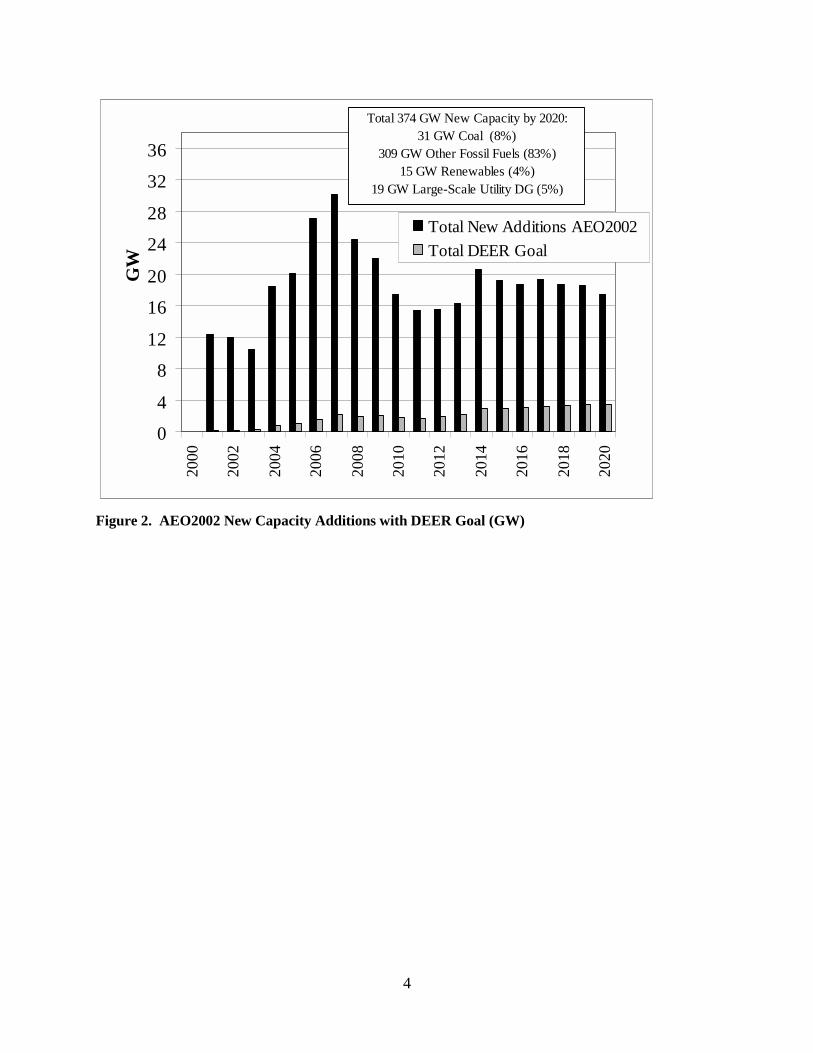
that is connected at distribution system voltages. The focus of this effort is on DG, comprising both smaller-scale DER-sized (� 1 MW) units in the residential and commercial sectors as well as larger-scale (� 1 MW) units in the commercial and utility sectors. It is illuminating to mention how the forecast provided by NEMS compares to the goal adopted by the Distributed Energy and Electric Reliability (DEER) office. The DG goal estimated by the DEER office at the time this report was written is to have 20 percent of all new generating capacity additions in 2020 be from DG sources. Using the AEO2002 projection of capacity growth, this goal can be quantified as follows. The AEO2002 forecasts 374 GW of required new capacity from electric generators and cogenerators by 2020. Of this, the AEO2002 estimates that 31 GW or 8% of the total will be from new coal with 309 GW or 83% from other fossil fuel sources. Only 15 GW is forecasted to come from renewables (or 4% of total new capacity), and the remaining 19 GW (5% of the total new capacity) is forecasted to come from large-scale utility-owned DG. An additional 3 GW of DER from small-scale residential and commercial sector installations is included in the renewables or gas-fired new capacity forecast, which brings the total to 22 GW. This DG number represents electricity-generating capacity only, and does not include CHP capacity forecasts. Based on the AEO2002 projections for new capacity additions, Berkeley Lab interprets the DEER goal to imply approximately 40 GW of new DG capacity must be installed by 2020. Figure 2 helps illustrate how 40 GW is calculated from AEO2002’s forecast of 374 GW of new capacity. The black shading represents the additional capacity installed each year by electric generators and cogenerators. The black bar magnitudes, which sum to 374 GW, come directly from the AEO2002 forecast. The DEER goal is located to the right of the AEO forecast in gray denoting the share of total new capacity that is expected to come from DG sources. Berkeley Lab calculates the values for the solid gray bars based on the assumption that DEER’s goal means that 20 percent of capacity installed in 2020 will be from DG, not that DG will contribute 20 percent of all cumulative new capacity between 2000 and 2020. Therefore, the solid gray bars show the interpolated DEER goal assuming 1 percent of new capacity in 2001 from DG, 2 percent of new capacity in 2002 and so forth up to 20 percent by 2020. The sum of all the solid gray bars, across all years, represents the DEER DG goal of approximately 40 GW. Note that a direct displacement of utility and cogenerator capacity by DG is assumed. That is, any effects of line losses, differential capacity factors, etc., are ignored.

4

0

4

8

12

16

20

24

28

32

36

2000

2002

2004

2006

2008

2010

2012

2014

2016

2018

2020

GW

Total New Additions AEO2002Total DEER Goal

Total 374 GW New Capacity by 2020:31 GW Coal (8%)

309 GW Other Fossil Fuels (83%)15 GW Renewables (4%)

19 GW Large-Scale Utility DG (5%)

Figure 2. AEO2002 New Capacity Additions with DEER Goal (GW)

5

2. How DG is Treated in NEMS

This section summarizes a paper by EIA staff (Boedecker et al. 2000) describing how DG is modeled in NEMS and also summarizes the model documentation (Energy Information Administration 2001b; Energy Information Administration 2001c). NEMS considers DG in both the residential and commercial buildings sectors, with some minimal treatment of DG in the utility sector. The DG module is designed to forecast electricity generation, fuel consumption and waste heat recovery for a variety of DG technologies. Berkeley Lab found that DG in NEMS is structured in a somewhat rudimentary manner, likely due in part to its relatively recent incorporation into the model. The penetration for new DG into these two sectors is dependent on a cash-flow analysis that determines economic attractiveness. Caps limit penetration of DG into new and existing buildings. 2.1 Overall Structure of DG Submodule

Figure 3 shows a flowchart that summarizes how the DG submodule is structured and shows what information is passing in and out of the submodule. This flowchart was adapted from a figure in the NEMS commercial module documentation (Energy Information Administration 2001b). At the top of the flowchart, two DG technology input files, one for the residential sector and the other for the commercial sector, provide the cost and performance data for each DG technology, financing assumptions, any applicable tax incentives, and any non-economic, program-driven exogenous penetrations of DG. This technology information is used in the cash flow analysis. The submodule reads in the electricity and natural gas prices from the NEMS supply-side modules at the census division level. Residential and commercial housing starts and stocks at the census division level are also passed into the model to determine the amount of new and existing construction available for potential DG penetration. Although NEMS accounts for both DG purchases to new construction as well as retrofits to the existing housing stock, the submodule focuses mainly on additions to new construction. According to the documentation, estimating the costs associated with retrofitting an existing building carries costs too complex to be generalized in NEMS (Energy Information Administration 2001b). Upper limits are set on DG penetration in both new and existing buildings, but the submodule ensures minimal DG installations in the existing housing stock by imposing a much stricter limit on the amount of DG deployment. The available housing starts and stock are used along with the results from the cash flow analysis and passed into the penetration function, which uses a logistic curve to determine the share of buildings that will adopt DG. The submodule then tallies up the amount of DG installed and determines whether there is any excess waste heat that can be used to supply water heating or space heating demand. There is no consideration of thermally activated cooling. The average electricity and hot water consumption is used to determine building fuel demand that DG can offset. Additionally, the submodule checks if excess DG generation is available for sales back to the grid. The DG submodule passes back electricity sales to the grid to the Electricity Market Module (EMM) and the natural gas requirements for DG back to the appropriate building sector. The remainder of this section will discuss in more detail many of these submodule characteristics.

6

RDGENTK/KGENTKinput file

DG equip cost & performance data,financing assumptions, tax

incentives, program-driven links

CASH FLOW ANALYSISCalculate # years to positive cash flow

Electricityand NaturalGas Prices

from Supply-side modules

DG EQUIPMENT ACCOUNTINGBy CD and General Characteristics

LOGISTICPENETRATION

FUNCTIONfor new construction

LOGISTIC RATEfor existingconstruction

UnitsInstalled for

NewConstruction

UnitsInstalled for

ExistingConstruction

Housing Startsby CD from

MAM

Housing Stockby CD from

RSDM/CSDM

AvgEnergyCons by

CD

WaterHeatingSuppliedby CD

Electricity Generatedand Consumed On-

Site by CD

Electricity Sales tothe Grid by CD

Natural Gas Needsfor DG by CD

Figure 3. Flow Chart of DG in NEMS’ Residential and Commercial Building Sectors

2.2 DG Technology Cost and Performance Data

Only two generic DG technologies are represented in the residential sector, solar photovoltaics (PV) and fuel cells, but capability to represent a third DG technology exists. The generic residential PV technology is sized at 2 kW with the fuel cell at 5 kW. A total of ten DG technologies are represented in the commercial sector. They are PV, natural gas fuel cells, natural gas or oil-fired reciprocating engines, gas or oil-fired turbines, gas microturbines, diesel engines, conventional coal, municipal solid waste (MSW) generators, biomass generators, and hydroelectric. The commercial DG technologies range in size from 10 kW, as represented by the commercial PV unit, up to 1500 kW for the biomass technology.

7

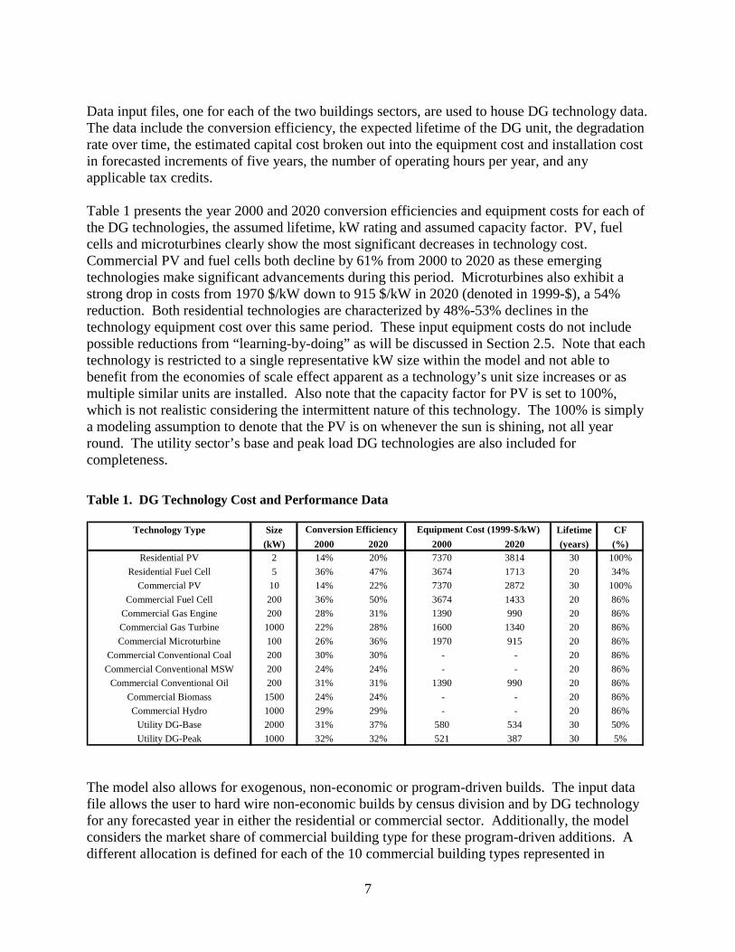
Data input files, one for each of the two buildings sectors, are used to house DG technology data. The data include the conversion efficiency, the expected lifetime of the DG unit, the degradation rate over time, the estimated capital cost broken out into the equipment cost and installation cost in forecasted increments of five years, the number of operating hours per year, and any applicable tax credits. Table 1 presents the year 2000 and 2020 conversion efficiencies and equipment costs for each of the DG technologies, the assumed lifetime, kW rating and assumed capacity factor. PV, fuel cells and microturbines clearly show the most significant decreases in technology cost. Commercial PV and fuel cells both decline by 61% from 2000 to 2020 as these emerging technologies make significant advancements during this period. Microturbines also exhibit a strong drop in costs from 1970 $/kW down to 915 $/kW in 2020 (denoted in 1999-$), a 54% reduction. Both residential technologies are characterized by 48%-53% declines in the technology equipment cost over this same period. These input equipment costs do not include possible reductions from “learning-by-doing” as will be discussed in Section 2.5. Note that each technology is restricted to a single representative kW size within the model and not able to benefit from the economies of scale effect apparent as a technology’s unit size increases or as multiple similar units are installed. Also note that the capacity factor for PV is set to 100%, which is not realistic considering the intermittent nature of this technology. The 100% is simply a modeling assumption to denote that the PV is on whenever the sun is shining, not all year round. The utility sector’s base and peak load DG technologies are also included for completeness. Table 1. DG Technology Cost and Performance Data

Technology Type Size Lifetime CF(kW) 2000 2020 2000 2020 (years) (%)

Residential PV 2 14% 20% 7370 3814 30 100%Residential Fuel Cell 5 36% 47% 3674 1713 20 34%

Commercial PV 10 14% 22% 7370 2872 30 100%Commercial Fuel Cell 200 36% 50% 3674 1433 20 86%

Commercial Gas Engine 200 28% 31% 1390 990 20 86%Commercial Gas Turbine 1000 22% 28% 1600 1340 20 86%Commercial Microturbine 100 26% 36% 1970 915 20 86%

Commercial Conventional Coal 200 30% 30% - - 20 86%Commercial Conventional MSW 200 24% 24% - - 20 86%

Commercial Conventional Oil 200 31% 31% 1390 990 20 86%Commercial Biomass 1500 24% 24% - - 20 86%Commercial Hydro 1000 29% 29% - - 20 86%

Utility DG-Base 2000 31% 37% 580 534 30 50%Utility DG-Peak 1000 32% 32% 521 387 30 5%

Conversion Efficiency Equipment Cost (1999-$/kW)

The model also allows for exogenous, non-economic or program-driven builds. The input data file allows the user to hard wire non-economic builds by census division and by DG technology for any forecasted year in either the residential or commercial sector. Additionally, the model considers the market share of commercial building type for these program-driven additions. A different allocation is defined for each of the 10 commercial building types represented in

8

NEMS. That is, depending on which DG technology is adopted, the share allocated to the commercial building types varies. The various commercial building types include education, assembly, food sales, food services, health care, lodging, large offices, small offices, merchant services, and warehouses. For example, for commercial fuel cells, 70% of DG forced builds are allocated to large office buildings, with 10% each distributed to education and healthcare type buildings, and the remaining 10% split between lodging and small offices. Berkeley Lab extracted the DG cost data and derived estimated levelized costs for each of the residential and commercial DG technologies exogenous to the model for technology purchases made in five different forecast years. Some assumptions that were made to calculate these costs include an assumed 12.5-year term for the loan, an interest rate of 6.5% real, and capacity factors assumed in the NEMS DG input file, which in most cases were 86%. Figure 4 illustrates the forecasted levelized costs of electricity for the various DG technologies. Conventional MSW, hydro, biomass, and conventional coal DG technologies were not included because the input file contained no cost information. The reason for this, EIA states, is because the model does not forecast growth in these technologies, although existing units are accounted for. The most expensive DG technology is residential and commercial PV, which for the most part, is not even displayed on this scale because the costs are so much higher than any other DG technology. The PV cost is estimated at 53 ¢/kWh in year 2000, with rapid declines throughout the forecast period to approximately 22 ¢/kWh in year 2020 for the commercial PV unit and 28 ¢/kWh for the residential PV unit in the final forecast year. Some of the more competitive DG technologies include microturbines, fuel cells, conventional oil, and gas engines, which are forecasted to be around 10 ¢/kWh by year 2020.

Levelized Cost of DG technologies (as input 86% CF)

0.0

10.0

20.0

30.0

40.0

1990 1995 2000 2005 2010 2015 2020

c/kW

h

Commercial PVCommercial Fuel CellCommercial Gas EngineCommercial Conv OilCommercial Gas TurbineCommercial MicroturbineResidential PVResidential Fuel Cell

Figure 4. Levelized Cost of DG technologies in NEMS

9

2.3 Cash Flow Analysis

The adoption rate of DG in new and existing construction is determined by how quickly an investment in DG takes to recoup its costs. For each potential DG purchase in either the commercial or residential sector, a 30-year cash flow analysis is performed. This calculation includes both costs and returns and consists of a down payment amount, which is assumed to be 20% of the capital cost, loan payments, maintenance costs, and fuel costs. The returns include energy cost savings, tax deductions, and any applicable tax credits. According to EIA, the main advantage of a cash-flow analysis approach versus a simple payback approach, i.e. the investment cost divided by the estimated savings, is the inclusion of financing assumptions (Energy Information Administration 2001b; Energy Information Administration 2001c). The added consideration of financing has the advantage of potentially yielding a faster positive payback. The reason for using a cash-flow approach is assuming that the investment in DG is rolled into the mortgage of the residential or commercial building. The result is the number of years required to reach a positive cash flow. If the net return is positive, the cumulative net cash flow increases. In some cases, the cash flow is never positive and the number of years is set to 30. 2.3.1 Tax Incentive Capabilities

The DG module also incorporates the benefits of tax credits when DG is purchased. If tax credits apply, they are applied as a one-time payment in the second year of the investment as part of the 30-year cash flow calculation. This assumes an average one-year waiting period is required in order to receive the credit. Sensitivity exercises of the tax credit indicate that a tax incentive can provide a significant boost to the potential of various DG technologies in the buildings sectors by quickly reducing the number of years required to obtain a positive cash flow. 2.4 Penetration Rate of DG Adoption

The number of years to produce a positive cash flow is then input to a penetration function. This function exhibits a logistic shape, with slow initial penetration followed by rapid growth and then finally a tapering off. The number of years to a positive cash flow is the primary determining factor for penetration, although a ceiling rate is arbitrarily imposed. The penetration characteristics are specific to each DG technology. This means that each technology has its own penetration potential based on the number of years to a positive cash flow. DG technologies therefore do not compete against each other in NEMS for a fixed amount of DG capacity. The model sets a maximum penetration parameter of 30% of all new construction for certain technologies in any one year. This maximum 30% applies to PV, fuel cells, gas engines, gas turbines, and microturbines and is static throughout the forecast period. In the residential sector, this 30% cap approximately results in a maximum possible penetration (corresponding a 1-year payback period) of 23,800 MW of PV and 59,500 MW of fuel cells given that 30% is installed over the forecast horizon to the maximum 30% of all new housing starts in NEMS. The remaining DG technologies only have a maximum 1% penetration rate per year in new housing. For retrofits of DG to existing construction, the penetration is even more limited to the lesser of 0.25% or one-fiftieth of the penetration rate into new construction. Under this constraint, residential DG is only able to install a maximum 440 MW of PV and 1,100 MW of fuel cells by

10

2020. This penetration constraint applied to potential DG purchases as retrofits to the existing housing stock significantly hinders the potential benefits of DG in this market share. Table 2 shows the maximum penetration rates for each of the residential and commercial DG technologies assuming the cash flow analysis yields a 1-year positive payback. For longer paybacks, the maximum penetration rate is further reduced, as seen Figure 5 where the maximum penetration rate falls from 30% to 10% as the payback increases from 1 year to 3 years.

Table 2. Maximum Penetration Rates for DG Technologies Given a 1-Year Payback*

Technology Type New Residential

New Commercial

Existing Residential

Existing Commercial

Residential PV 30% - 0.25% -Residential Fuel Cell 30% - 0.25% -

Commercial PV - 30% - 0.25%Commercial Fuel Cell - 30% - 0.25%

Commercial Gas Engine - 30% - 0.25%Commercial Gas Turbine - 1% - 0.02%Commercial Microturbine - 30% - 0.25%

Commercial Conventional Coal - 1% - 0.02%Commercial Conventional MSW - 1% - 0.02%

Commercial Conventional Oil - 1% - 0.02%Commercial Biomass - 1% - 0.02%Commercial Hydro - 1% - 0.02%

* All penetration rates will be lower if the cash-flow calculation yields a longer payback and for retrofits is estimated to be the lower of 0.25% or 1/50 of the maximum penetration rate to new construction Figure 5 illustrates the logistic shape of the penetration function of various example positive payback periods assuming the maximum 30% penetration as taken from the EIA documentation of the DG module. Again, the 30% maximum penetration only applies to new installations of PV, fuel cells, gas engines, gas turbines, and microturbines, with the other DG technologies further constrained as seen in Table 2. Figure 5 illustrates the logistic pattern of DG penetration to new construction, as characterized by slow initial growth, followed by a period of more rapid penetration, and ending with a leveling effect over time. In this example, given a 1-year positive payback, the penetration function shows a steep and optimistic shape in the logistic function to the maximum 30% penetration of new construction by 2011. This represents the maximum annual penetration rate that a DG technology can have given an investment payback of 1-year or less and assuming the installation is occurring in new housing construction. A 3-year positive payback results in a dramatic flattening off of the logistic curve by 2012 at a maximum 10% penetration of new construction. The 10-year payback shows a slight penetration in the last ten years of the forecast up to approximately 2.5% of new construction per year in the last 5 years of the forecast. Above a 20-year payback, no noticeable DG penetration can be seen. These penetration caps are based on EIA’s simulations of the penetration function under a maximum assumed penetration of 30% for new construction.

11

0%

5%

10%

15%

20%

25%

30%

35%19

90

1995

2000

2005

2010

2015

2020

Pene

trat

ion

into

New

Con

stru

ctio

n 1 year3 years10 years20 years29 years

Penetration Function SimulationsFor Various Years Until a Positive Cumulative Cash Flow is Achieved

source: adopted from EIA’s documention on the DG submodule

Figure 5. Penetration Function Simulations

2.5 Learning-By-Doing

Learning-cost effects potentially affect the economic attractiveness and penetration rates of a DG technology, so learning-by-doing improvements are applied to newer, emerging DG technologies, i.e. PV, fuel cells and microturbines. Learning-by-doing reduces the capital costs as the technology matures over time. As a result, the forecasted DG capital costs may be lower than the input technology cost due to learning-by-doing and the increased deployment over time as the technology progresses along the logistic penetration function. Learning-by-doing is designed to determine the minimum between the DG technology cost that was used in the DG input file and the endogenous cost that may have changed during the forecast due to learning. The following shows the mathematical representation of learning-by-doing in NEMS. equipmentcost = min{menucost, c0*cumship-beta} The installed DG equipment cost is lowered from the menu cost or the initial input file cost under the influence of learning cost parameters (c0 and beta) and the cumulative shipments (cumship). Beta is the learning parameter, which determines the sensitivity of cost changes to cumulative shipments. This value is the assumed maximum penetration for each DG technology. Since c0 (also called alpha) or first unit costs are generally unobservable, the learning functions calculate a value for first unit cost that calibrates to the current installed costs for the technology given current cumulative shipments and the assumed value of beta. 2.6 Utility Sector DG

NEMS also treats DG penetration in the utility sector, although only very generally. DG was incorporated into the Electricity Market Module (EMM) in the AEO2001 version of NEMS to

12

represent DG that is owned by electricity suppliers, not the consumer-owned DG that is modeled in the buildings sectors (Energy Information Administration 2002). DG in the EMM is characterized separately into construction designed to serve base and peak loads. DG in this sector considers the construction, operation, and avoided T&D costs associated with new adoption. The DG is operated according to a pre-determined utilization rate based on potential supply. The utilization rates of the base and peak load DG is assumed to be 50% and 5%, respectively. The cost and performance data for the DG technologies in the utility sector was provided by Distributed Utility Associates Group. Only two generic DG technology options are available, one for base load demand and the other for peak load demand. DG is generally more expensive for simple cycle electricity production than central station plants, but are generally cheaper than the residential or commercial DG costs (Energy Information Administration 2002) due to the larger size of between 1-2 MW and conventional nature of the technology. DG adoption in the utility sector is accounted for by region and by year. Utility sector DG also takes into account the avoided cost of new T&D equipment. This cost is accounted for by region and depends on the distribution of the load. As such, the cost of adding T&D equipment can vary considerably, depending on the location of the load (Energy Information Administration 2002).

13

3. Sensitivity Exercises

Based on the understanding of how the DG module works that is described above, a series of sensitivity cases were performed. This section describes a set of sensitivity cases that Berkeley Lab ran to mimic the cases discussed in Boedecker et al. using the AEO2002 version of NEMS as well as Berkeley Lab’s own set of sensitivity runs of the DG capabilities in NEMS. 3.1 EIA’s DG in the Buildings Sector Sensitivity Cases

In 2000, Boedecker et al. analyzed the sensitivity of DG in the AEO2000 version of NEMS by offering some alternative cases involving enhanced DG assumptions. This section discusses the results from each of the cases presented in the analysis using the newer AEO2002 version of NEMS. The results indicate that enabling net metering or increasing tax incentives has a more positive effect on DG installation than lowering the technology costs of fuel cells and PV, but reducing the costs of conventional technologies that are closer to being competitive has a significant effect. In general, the results using the AEO20002 version of NEMS do not differ significantly from the AEO2000 analysis due to minimal changes to the model in this timeframe with respect to DG effects. A total of six alternative DG cases were performed to roughly replicate Boedecker et al.’s analysis using the most recent version of NEMS. Table 3 below summarizes the results from the various scenarios that Boedecker et al. originally modeled and Berkeley Lab replicated. This table represents the generation increase from various DG technologies in the commercial and residential sectors along with the reduction in carbon emissions from the electric utility sector. Table 4 is also provided to present the total installed DG capacity for each of the six cases. Figure 6 is provided to illustrate the forecasted change in carbon emissions from the electric utility sector for each of the cases over time. Results are discussed for each of the cases in the following subsections.

Table 3. Change in DG Generation (TWh) and Carbon Emissions (Mt) in Buildings Sector in Year 2020 Relative to AEO2002 Reference Case with % Differences

Case PV Fuel Cells Microturbine Other DG Total DG Carbon Emissions

Case 1 - Adv. Technology Costs 3.3 (333%)

2.6 (30%)

7.8 (113%)

0 (0%)

13.7 (50%)

-2.7 (-0.3%)

Case 2 - Net Metering 0 (0%)

72.1 (815%)

9 (131%)

18.6 (170%)

99.6 (361%)

-5.7 (-0.7%)

Case 3 - Adv Costs and Net Metering 3.2 (330%)

71.3 (806%)

24.3 (353%)

17 (159%)

115.8 (420%)

-6.2 (-0.8%)

Case 4 - 40% Fuel Cell and PV Tax Credit and Adv Costs

19.3 (1968%)

77.8 (880%)

7.6 (111%)

-0.1 (-0.9%)

104.6 (379%)

-11.7 (-1.5%)

Case 5 - 40% Fuel Cell Tax Credit and Adv Costs

3.3 (333%)

78.5 (888%)

7.6 (111%)

-0.1 (-0.9%)

89.3 (324%)

-10.1 (-1.3%)

Case 6 - 40% PV and all Gas-Fired Techs Tax Credit and Adv Costs

19.3 (1968%)

77.7 (879%)

21.9 (319%)

10 (92%)

128.8 (467%)

-15.4 (1.9%)

14

Table 4. Total Installed DG Capacity (MW) in Buildings Sector by Year 2020 from AEO2002

Case PV Fuel Cells Microturbine Other DG1 Total DG

AEO2002 Reference Case 461 1,215 969 1,520 4,166

Case 1 - Adv. Technology Costs 2,058 1,580 2,068 1,516 7,223

Case 2 - Net Metering 462 12,057 2,240 4,107 18,866

Case 3 - Adv Costs and Net Metering 2,043 11,911 4,395 3,890 22,239

Case 4 - 40% Fuel Cell and PV Tax Credit and Adv Costs 10,096 17,648 2,046 1,515 31,304

Case 5 - 40% Fuel Cell Tax Credit and Adv Costs 2,059 17,839 2,047 1,514 23,460

Case 6 - 40% PV and all Gas-Fired Techs Tax Credit and Adv Costs 10,096 17,670 4,068 2,902 34,736

1Other DG includes gas engines, gas turbines, conventional coal, conventional MSW,conventional oil, biomass, and hydropower

Difference in Carbon Emissions from Electric Generators (Mt)

-20-18-16-14-12-10

-8-6-4-202

2000 2005 2010 2015 2020

Mt

Case 1 - Adv. Technology CostsCase 2 - Net MeteringCase 3 - Adv Costs and Net MeteringCase 4 - 40% Fuel Cell and PV Tax Credit and Adv Costs

Case 5 - 40% Fuel Cell Tax Credit and Adv CostsCase 6 - 40% PV and all Gas-Fired Techs Tax Credit and Adv Costs

Figure 6. Difference in Total Carbon Emissions from Electric Generators (Mt)

15

3.1.1 Case 1: Advanced Technology Cost Assumptions

Case 1 assumes an approximate 20-30% reduction in the capital cost of emerging DG technologies, namely PV, fuel cells, and microturbines, by the last five years of the forecast. Table 5 below shows the change in the DG technology costs with the AEO2002 costs to the left of the arrow and the advanced technology costs to the right of the arrow in each forecasted period. The PV capital costs show the strongest improvements, down almost 28% by 2020 relative to the AEO2002 version of NEMS with fuel cell capital costs reduced by 25% in the last five years of the forecast. Natural gas microturbine capital costs are forecasted to have 20% lower costs from 2015-2020, a reduction from 700 $/kW to 560 $/kW in these same years. The efficiencies of each of these technologies were unchanged in this case from the AEO2002 reference case.

Table 5. Advanced Technology Case Installed Costs for DG Technologies (1998-$/kW)

Source: Adapted from EIA’s Modeling Distributed Generation in the NEMS Buildings Models paper The results from this run are shown in Table 3 and 4. Using the AEO2002 version of NEMS, this advanced technology cost case results in 13.7 TWh more DG generated in the buildings sectors relative to the AEO2002 reference case for a total of 27.6 TWh by 2020. The additional 13.7 TWh is dominated by a 7.8 TWh increase from microturbines, with roughly 3 TWh each from PV and fuel cells. Table 4 provides the installed DG capacity impacts for each case, denoting a 73% increase in DG capacity from 4.2 GW to 7.2 GW by 2020. Carbon emissions from electric generators are only reduced by 2.7 Mt by 2020 in the buildings sectors. Some possible reasons for this modest result, EIA notes, is that although the capital cost is lower in this scenario, the reference case also forecasts significant declines in costs. Also, the electricity price is decreasing over time in the reference case version of the model, disadvantaging the economic attractiveness of DG deployment. 3.1.2 Case 2: Net Metering

Case 2 estimates the value of grid sales at the retail electricity rate. Net metering is permitted for PV as well as all natural-gas fuel-consuming DG technologies in the residential and commercial sectors in this case. The reference case version of the model assumes net metering for PV only. This scenario determines the benefits of net metering to all other natural gas-consuming DG technologies, rather than at the estimated marginal cost of generation or lower-than-retail price. The net metering option increases the incentive for DG generation above what is needed by the end-user.

DG Technology 2000-2004 2005-2009 2010-2014 2015-2020

Residential and Commercial PV 5529 to 5529 (0% reduction)

4158 to 3840 (28% reduction)

3178 to 3000 (6% reduction)

2426 to 1750 (28% reduction)

Residential and Commercial Fuel Cell 3625 to 3625 (0% reduction)

3000 to 2400 (28% reduction)

2425 to 1940 (20% reduction)

1725 to 1293 (25% reduction)

Commercial Microturbine 800 to 800 (0% reduction)




16

The results from this case indicate that net metering has a much greater impact on DG penetration than the advanced technology cost assumptions in Case 1. Total DG is up 100 TWh by 2020, with over 72 TWh of the total coming from fuel cell generation increases. Microturbines show a 9 TWh increase in this case. No change in PV is evident in this case because the AEO2002 Reference Case already accounts for net metering from PV units. Net-metering results in 14.7 GW more DG compared to the AEO2002 reference case in 2020, with 10.8 GW of this from fuel cells. The additional generation from fuel-based DG technologies results in a 5.7 Mt drop in carbon emissions from the utility sector with a 4.5 Mt increase in the buildings sectors. This increase is more than compensated by a decrease in emissions from the utility sector. 3.1.3 Case 3: Net Metering with Advanced Technology Cost Assumptions

Case 3 simply combines the assumptions made in Cases 1 and 2, allowing for net metering of all fuel-based technologies in conjunction with the advanced technology cost assumptions. The results shown in Table 3 are not that different than the sum of the previous two case results. The total increase in DG generation is just over 115 TWh by 2020. Of this, roughly 71 TWh is from fuel cells. Microturbines seem to benefit from having both sets of assumptions in place, resulting in over 24 TWh in 2020, more than the sum of Cases 1 and 2. Table 4 shows over 18 GW more DG from the buildings sector in 2020, coming largely from fuel cells and microturbines. Again, carbon emissions decrease by 6.2 Mt in 2020 from the utility sector and are compensated with an increase in the buildings sectors of 4.8 Mt, which is not too different to Case 2. 3.1.4 Case 4: 40% Fuel Cell and PV Tax Credit with Advanced Technology Costs

EIA also analyzed the proposed Climate Change Technology Incentive (CCTI) for FY 2001. This proposal included two tax credits with lowered DG capital costs. One was a 20% incentive for fuel cells and the other a 15% credit for PV. Both credits were reductions from the installed cost, with the fuel cell tax credit imposing a limit of 500 $/kW from 2001 to 2004 and the PV incentive capped at a $2000 total between 2001 and 2007. However, according to EIA, this scenario resulted in very little DG deployment because EIA believes the magnitude and time horizon of the tax credits was too small or short. Therefore, this scenario was not replicated here. Instead EIA opted to model a more aggressive alternative scenario, which is replicated by Berkeley Lab in this analysis. Case 4, the more aggressive scenario to the proposed CCTI, imposed a stronger 40% tax incentives for PV and fuel cells than the CCTI analysis, coupled with the Case 1 advanced technology costs. The reason for coupling both a tax incentive and lowered technology costs is that the 40% tax credit is believed to result in advancements in the DG production costs, warranting the inclusion of lowered cost assumptions. No monetary limit is placed on the amount of either credit that can be received and the incentives are in place through year 2020. The net effect of this alternative scenario is less than Case 3, indicating that net metering has a stronger impact on DG than the imposed 40% tax incentives to PV and fuel cells. With a 40% tax credit given to PV and fuel cells in addition to the advanced technology costs, over 104 TWh

17

of energy comes from DG by 2020, over 77 TWh of this is from fuel cells, indicating the benefits of both lowered costs and generous tax incentives to this nascent technology. PV is up 19.3 TWh by 2020, with nearly 8 TWh more from microturbines. With respect to installed DG capacity, the increase is more than Case 3 due to a large increase in fuel cell and PV capacity that more than offsets the lower capacity from microturbines and other DG technologies compared to Case 3. Carbon emissions from electric generators are down 11.7 Mt in this scenario by 2020. 3.1.5 Case 5: 40% Fuel Cell Tax Credit with Advanced Technology Costs

Case 5 is similar to Case4 with the exception that only the fuel cell tax credit is incorporated. This case is performed to separate the resulting benefits from each of the tax credits. Without the presence of a PV tax credit, fuel cells generate 79 TWh more than the AEO2002 reference case, only slightly higher than Case 4, however. This demonstrates that competition among DG technologies in the buildings sectors is nonexistent in the NEMS model. Without the PV tax credit, carbon emissions from the utility sector are only reduced 10.1 Mt, 1.6 Mt less than Case 4 in 2020. Capacity additions are 8 GW lower than Case 4 due to the absence of the PV tax incentive in 2020. 3.1.6 Case 6: 40% Tax Credit for PV and all Gas-Fired Technologies with Advanced

Technology Costs

Case 6 forecasts very aggressive incentives to DG. In this case, the 40% tax credit is not only applied to fuel cells and PV, but to all other gas-fired DG technologies. Also, the Case 1 advanced technology cost assumptions are applied. This case broadens the scope of assumptions to benefit the conventional DG technologies as well as those still emerging onto the market. Results from this case show the most DG penetration of the six cases EIA analyzed, with generation from DG is up nearly 129 TWh by 2020. Again, a large share of this increase is from fuel cells, 78 TWh over the AEO2002 reference case. PV increases are similar to Case 4, up 19 TWh by 2020. Microturbines show a notable increase as a result of the added tax incentive, up 22 TWh in this case. This can be explained by comparing the results to Case 4, which did not include the tax incentive to gas-fired DG technologies. Compared to Case 3, however, which resulted in 24.3 TWh more generation from microturbines, the net benefit is slightly lower with a 40% tax credit compared to enabling net metering. DG capacity additions are the greatest of all six cases, with 31 GW more relative to the AEO2002 reference case. Comparing all six cases, this scenario resulted in the lowest carbon emissions in the utility sector, down 15.4 Mt by 2020. 3.1.7 Summary of EIA’s DG Sensitivity Analysis

The series of EIA sensitivity assumptions provides a lot of insight into what factors could be effective at enhancing DG penetration over the next two decades. This study produced a wide range of optimistic outlooks. The following summarizes the findings from this analysis: • A 20-30% reduction in the PV, fuel cell, and microturbine capital costs by 2020 result in

modest DG penetration. For these young technologies, the costs are still far above the threshold for competitiveness. Even this seemingly significant reduction is not enough to

18

make DG economically attractive in NEMS. Additionally, the AEO2002 reference case exhibits capital cost declines over time, which could already be capturing some portion of the incremental penetration from lowered costs.

• Enabling net metering for fuel-based DG technologies produces slightly more DG penetration compared to imposing PV and fuel cell 40% tax incentives when advanced technology costs are assumed. In Cases 3 and 4, the 11 TWh difference (116 TWh versus 105 TWh) by the final forecast year indicates the slight advantage of net-metering over the imposed tax incentives. In both cases, fuel cell penetration covers a majority of the added benefits. The main difference seems to be due to the fact that microturbines receive more of a boost from net metering than PV receives from a 40% tax credit.

• Fuel cells seem the most receptive to net metering or aggressive tax incentive enhancements, indicating that cost reduction does little to further DG deployment in NEMS. A 25% reduction in capital cost was not substantial enough to motion further adoption beyond the AEO2002 reference case.

• Microturbines are moderately responsive, but only when net metering is enabled and capital costs are decreased or subject to a 40% tax credit, as in Case 6.

• PV benefits are modest with the only notable increase from the tax credit. The 28% reduction in capital costs does very little to stimulate PV growth. Because the reference case already accounts for net metering, no incremental change from Case 2 is noticeable.

The following section looks further at the sensitivity of DG parameters. Berkeley Lab developed a series of runs that cover the range of results based on forced exogenous builds, reduced DG technology capital costs beyond what EIA assumed, and various tax incentives for selected DG technologies. 3.2 Sensitivity of Various DG Capabilities in NEMS Building Sectors

A series of runs exercised the sensitivity of selected DG-related parameters in NEMS to determine whether certain parameters have a greater impact on DG than others. The parameters chosen for this work were forced exogenous builds, lowered technology costs and enhanced tax incentives. The purpose of doing these runs was to see whether these selected parameters were significant barriers to widespread DG deployment. To perform these runs, modifications were made to the residential (rgentk) and commercial (kgentk) DG input files. A set of runs were performed to represent a broad range of outcomes for a given parameter change. Results showed that realistic technology characteristic enhancements or legislated subsidies did little to stimulate DG growth in NEMS. Results were interesting only when modifications were beyond what seemed reasonable for policy initiatives or tax incentives. The following subsections describe in detail the various sensitivity runs that were done for each of these three parameters along with some discussion of the results. 3.2.1 Exogenous Penetrations

Exogenous penetrations were considered for selected commercial and residential DG technologies. In the residential sector, forced builds were made to PV and fuel cells, and

19

commercial sector exogenous penetrations were applied to PV, fuel cells and microturbines. The exogenous penetration or forced build sensitivities represent hard-wired DG installations to the model. These technologies were chosen for this exercise because they offer promising improvements over the next two decades, the forecast horizon of NEMS. A series of runs were performed by multiplying the default reference case exogenous penetration for PV, fuel cells and microturbines by varying degrees, e.g. 10x, 100x, 150x, 200x, and 1000x. The 1000x case unfortunately was too extreme for NEMS, as the model crashed early in the model run. The goals of this exercise were to ensure that exogenous penetrations could be forced in the model, determine the upper limits of NEMS ability to add forced builds, and assess the impacts on the utility sector with varying magnitudes of forced DG builds. Table 6 below summarizes the results from this set of runs. Table 6. Results from Exogenous Penetration Runs for Year 2020 Relative to AEO2002

Case

Increase in Total

Res/Comm DG (TWh)

Change in Total Installed Capacity (GW)

Change in Total Carbon Emissions

from Electric Generators (Mt)

Change in Electricity-

Related Losses (Quads)

10x AEO200213.4 -1.9 -2.3 -0.1

100x AEO2002121.6 -26.2 -15.2 -0.5

150x AEO2002178.9 -36.3 -19.0 -0.7

200x AEO2002 235.3 -48.1 -23.3 -0.9

Results from the first sensitivity run indicates that increasing exogenous penetration of DG by ten-fold does modestly increase the total amount of DG generation by 13 TWh by 2020, but does little to impact much else. Utility sector installed capacity is virtually unchanged, as are electricity-related losses, with total carbon emissions only reduced by a little over 2 Mt. With multiples of 100, 150, and 200 times over the AEO2002 exogenous builds, the impacts on the larger scale utility sector are more apparent. Enhancing the non-economic DG builds 100-fold increases total DG generation in the buildings sectors by nearly 122 TWh in 2020. As a result, carbon emissions go down by over 15 Mt with T&D related losses cut by only 0.5 Quad in 2020. The 200-times run roughly doubles the impacts from the 100-times scenario. In general, the results from this experiment indicated that although non-economic measures can stimulate DG growth in NEMS, it is likely not enough to significantly impact the utility sector outlook unless extreme values are assumed. Increasing the forecasted deployment of DG in the residential and commercial sectors by ten-fold above the AEO2002 reference case did little to alleviate the stress from the power sector. The following subsection presents the results from lowered DG equipment and installation costs in the buildings sector.

20

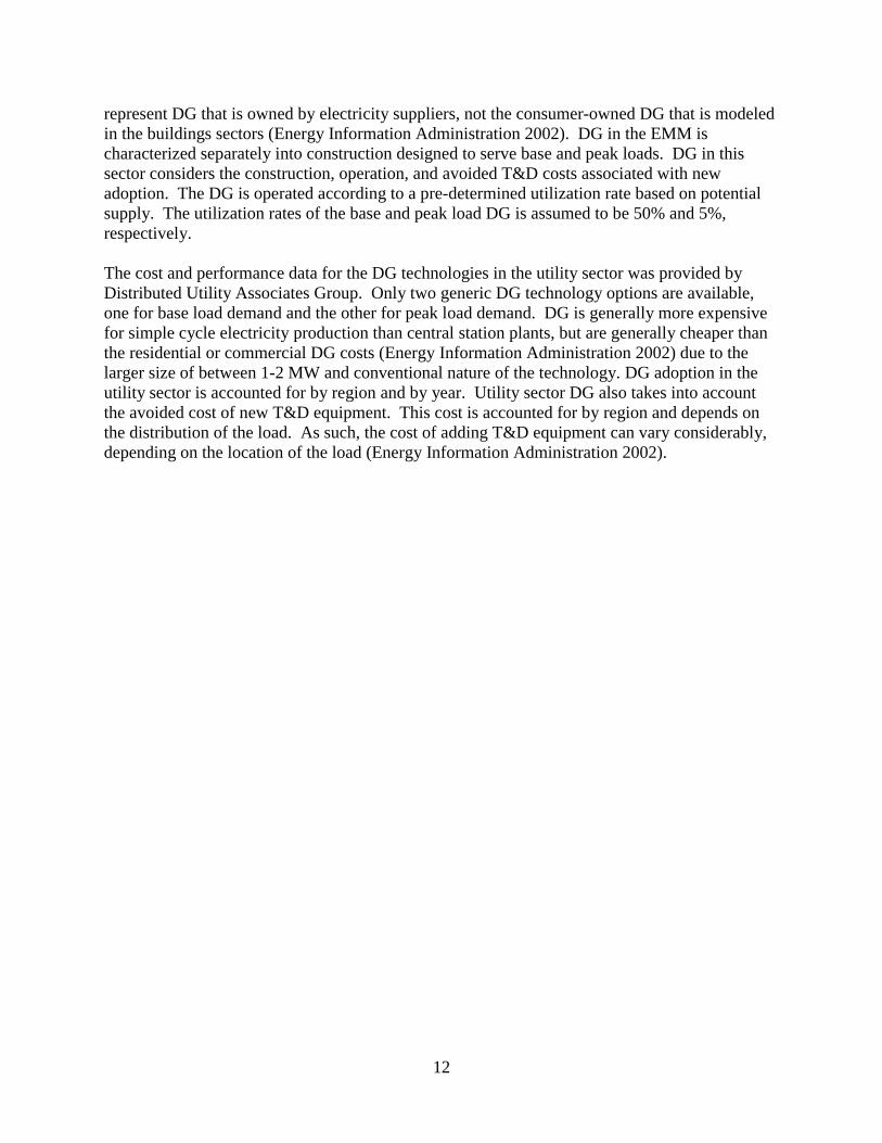
3.2.2 Lowered Capital Costs

Three different scenarios of lowered capital costs were modeled in this exercise. For these runs, the equipment and installation costs were lowered by specified percentages across all forecasted years. The lowered costs were applied to residential and commercial PV, fuel cells, and, commercial microturbine technologies. Berkeley Lab chose a series of 25%, 50%, and 75% reductions of the annual equipment and installation costs for all forecasted years. The results are presented in the table below, in a similar format to Table 6 above. Table 7. Results from Lowered Capital Costs Runs for Year 2020 Relative to AEO2002

Case

Increase in Total

Res/Comm DG (TWh)






25%6.0 -0.1 0.1 0.0

50%22.4 -0.6 -2.8 -0.1

75% 64.1 -5.5 -6.3 -0.3

In general, the results from significantly lowering the DG capital costs in NEMS are lower than imposing forced builds of the previous section. The results indicated that even with a 50% reduction in residential and commercial DG capital costs, DG growth is only modest. With total DG generation increasing by nearly 22 TWh in 2020 under these halved costs, utility sector capacity is hardly affected, down only a fraction of a GW. With a 75% reduction in the PV, fuel cell, and microturbine capital costs, DG generation is more significant, up over 64 TWh by 2020. However, total installed capacity in the power sector is only lowered 5.5 GW, with over 6 Mt of carbon emissions saved. The reason for this is likely due to the fact that the DG technology costs are already experiencing significant declines in the reference case and any further decrements to these costs are not as likely to produce significant effects. Thus, NEMS indicated that the emerging DG technologies, PV, fuel cells, and microturbines, would require more than just improved technology costs to significantly shift the reliance on the power sector for electricity. The following section presents additional sensitivities to using incentives below and above what was presented from EIA’s study to determine potential DG benefits. 3.2.3 Enhanced Tax Incentives

The third and final parameter that Berkeley Lab experimented with is tax credits. Based on the EIA analysis that modeled a 40% tax incentive on PV and fuel cells, this exercise further investigated the sensitivity of tax credits by varying the magnitude of the credit. Tax incentives of 10%, 25%, 50%, and 75% for residential and commercial PV and fuel cells were modeled.

21

The tax incentives imposed in these runs were assumed to apply to all forecasted years with no maximum monetary limit imposed. Table 8. Results from Enhanced Tax Incentive Runs for Year 2020 Relative to AEO2002

Case

Increase in Total

Res/Comm DG (TWh)






10%8.2 0.4 0.2 0.0

25%46.9 -5.8 -4.9 -0.2

50%134.0 4.2 -12.8 -0.5

75% 165.3 7.7 -16.7 -0.7 The results indicated that PV and fuel cell tax incentives have a greater impact on DG deployment than reduced technology costs. Although a 10% incentive does not result in significant DG benefits, the 25% subsidy shows moderate improvements in growth, with a 47 TWh increase in DG generation. This resulted in nearly 6 GW of avoided capacity by 2020 in the utility sector, with nearly 5 Mt of carbon emissions savings in the same year. With the 50% and 75% PV and fuel cell tax credits, the amount of DG deployment is much more attractive with between 134 TWh and 165 TWh of new DG generation, respectively. However, the amount of installed capacity in the power sector actually increases in these two cases, due to the high levels of natural gas fuel cells installed. Overall, carbon emissions are reduced, due to the displacement from coal to natural gas use with these imposed assumptions. Imposing a tax credit in NEMS makes DG more viable. Even with only a 25% incentive, changes in the power sector are noticeable. With the 50% and 75% tax credits, however, fuel cells really take off. Fuel cells are highly attractive in these cases, resulting in a large increase in natural gas cogeneration, as shown by the increase in capacity in the utility sector. However, because it is cogeneration, carbon emissions still result in savings over the AEO2002 reference case. 3.2.4 Summary of Berkeley Lab’s Sensitivity Runs

Figure 7 below summarizes how DG penetration increased for each of the sensitivity cases Berkeley Lab examined. Obviously, exogenous forced penetrations possessed the greatest potential to raise DG levels in the NEMS buildings sectors, although at extremely high magnitudes. Significant capital cost reductions that might be associated with accelerated technology improvements unfortunately did not stimulate DG growth as much. Tax incentives offer the potential for enhanced DG deployment with significant results seen in the 25%, 50%, and 75% tax credit scenarios.

22

Change in Buildings DG Generation

0

50

100

150

200

250

2000 2002 2004 2006 2008 2010 2012 2014 2016 2018 2020

TWh

10x Exog Penetration100x Exog Penetration150x Exog Penetration200x Exog Penetration25% Capital Cost Reduction50% Capital Cost Reduction75% Capital Cost Reduction10% Tax Credit25% Tax Credit50% Tax Credit75% Tax Credit

Figure 7. Change in Residential and Commercial DG Generation (TWh) from AEO2002 Reference Case

The following section presents possible alternatives and/or improvements to modeling DG in NEMS.

23

4. Alternative Method for DG Forecasting in NEMS

4.1 Introduction

As discussed above, the treatment of distributed generation in NEMS is fairly rudimentary. NEMS characterizes national energy demand sectors at the level of customer type and region, and thereby misses out on many niche markets for DG. There are a number of ways that the current structure of NEMS could be modified to better reflect DG market potential, leading to more credible estimates of DG penetration. These modifications can be organized into the following three categories: 1. Expand the potential markets for DG by broadening the customer and technology types that

are analyzed. For example, NEMS currently allows DG adoption in the residential and commercial sectors only, and misses out on key industrial applications.

2. Provide greater detail of DG system economics in the NEMS cash flow analysis. This includes consideration of the structure of retail electricity tariffs in greater detail, and refining input parameters that are averaged annually to reflect daily and annual variation in system operation, customer demand, and energy prices. An additional possible consideration is economies of scale at specific sites.

3. Incorporate geographical adoption parameters that are either not currently addressed in NEMS or are addressed on a scale that is too aggregated to properly represent their variation. Identifying local effects on DG adoption is one way to highlight niche DG markets.

The first two modifications are discussed briefly below and the third modification is discussed in more detail as a thought experiment on the type of modifications that would be required to fit an external analysis into the existing structure of the NEMS model. 4.2 DG Market Expansion

Enhancements that fall under the category of DG market expansion refer to broadening the technology types, customer types, and applications for DG that are currently considered in NEMS. Several possible modifications were discussed above in the scoping section of this report. Some key NEMS development areas that would expand the potential markets for DG are listed below, ordered according to the level of complexity required to program them into NEMS: 1. Raise the cap on maximum DG penetration rate for DG adoption in new construction. 2. Loosen the constraint on DG adoption by existing construction. Most notably, NEMS

currently allows for DG adoption by existing buildings, but the penetration level is set arbitrarily low, at a maximum of 0.25% per year of total available housing.

3. Expand the allowances for net metered technologies to match existing state laws. Wind systems and select thermal technologies are currently included in net metering programs of several states, but only PV is allowed in NEMS. Note that the NEMS reference cast is limited to the assumption that existing regulation persists for the forecast period. While net metering laws are in constant flux, only the current configuration could be applied as a reference case.

24

4. Increase the technology types considered for all sectors, including electricity generation from mobile sources, small wind generation for low-density regions, and solar-thermal generation. This would allow certain technologies to be adopted by niche markets where appropriate.

5. Expand the facilities that can adopt DG to include the industrial sector. Certain building types such as machine and repair shops, laundromats, and small-scale industry (i.e. less than 800 kW) are generalized under one of the commercial categories, but other small industries are aggregated with the industrial sector.

6. Enhance the representation of DG to cover more technologies and consider economies of scale in technologies.

7. Consider thermally activated cooling as a use of waste heat. 4.3 Improved Cash Flow Analysis

NEMS currently determines the future penetration of individual DG technologies based on the number of years required for each technology investment to reach a positive cash flow, which is roughly equivalent to a simple payback period. The cash flow calculation uses annual averages of economic and technology performance variables, and does not account for the dependence of system economics on technology operation schedules, specifically in daily and seasonal variation in demand or the temporal correlation between electric and thermal loads. In addition, NEMS inputs flat retail electricity rates where time-of-use or real-time rates may be applicable, does not consider demand charges for commercial buildings, and does not consider seasonal fluctuation of electricity or fuel prices. The financial impact of offset peak electricity use is therefore not included in the current cash flow analysis. This economic consideration is particularly important for commercial and industrial customers who are able to decrease high demand charges, often a significant portion of a customer’s monthly bill, by reducing their peak electricity load with DG. The cash flow analysis could be improved by integrating an external module to conduct a more detailed, technology-operation analysis of DG economics. Several DG analysis tools exist that simulate the operation of a DG system over a test year or the lifetime of the DG technology. Some examples include DER-CAM developed by Berkeley Lab, D-Gen Pro created by Architectural Energy Corp. (AEC) with support from the Gas Technology Institute, or DG Profiler developed by Jackson Associates. These models have the ability to analyze the relationship between customer load profiles and complex electricity tariffs instead of taking average values over a test year. Typical model inputs include customer load profiles (electricity, cooling, and heat demands), electric and gas tariff structures including energy charges, demand charges, and standby charges, and technology cost and performance data for a variety of DG technologies. In addition, certain models can account for policies such as air quality restrictions that influence the operation of DG technologies. The key outputs that could be derived from an external analysis are total customer electricity and gas consumption and cost, average cost of electricity (COE), and total heating and cooling demand offset by CHP technologies. These outputs, along with estimated technology lifetime and net capital cost will yield the number of years until a positive cash flow is reached for a specific forecast year when the technology is purchased.

25

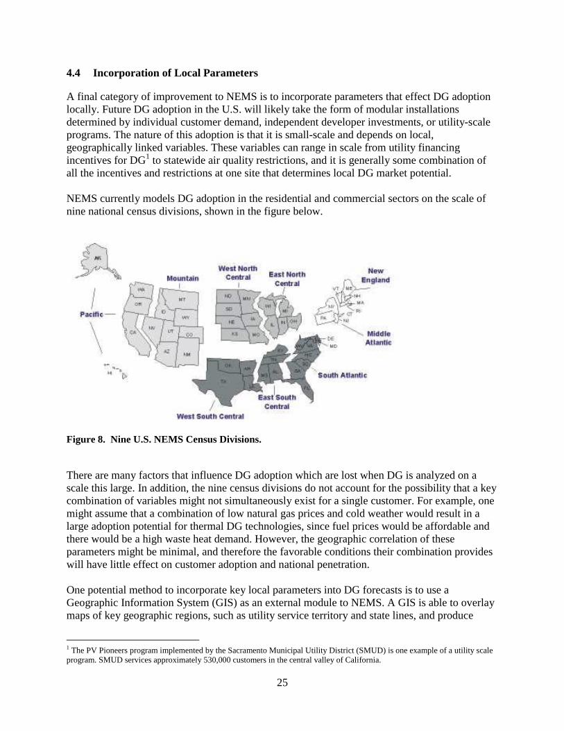
4.4 Incorporation of Local Parameters

A final category of improvement to NEMS is to incorporate parameters that effect DG adoption locally. Future DG adoption in the U.S. will likely take the form of modular installations determined by individual customer demand, independent developer investments, or utility-scale programs. The nature of this adoption is that it is small-scale and depends on local, geographically linked variables. These variables can range in scale from utility financing incentives for DG1 to statewide air quality restrictions, and it is generally some combination of all the incentives and restrictions at one site that determines local DG market potential. NEMS currently models DG adoption in the residential and commercial sectors on the scale of nine national census divisions, shown in the figure below.

Figure 8. Nine U.S. NEMS Census Divisions.

There are many factors that influence DG adoption which are lost when DG is analyzed on a scale this large. In addition, the nine census divisions do not account for the possibility that a key combination of variables might not simultaneously exist for a single customer. For example, one might assume that a combination of low natural gas prices and cold weather would result in a large adoption potential for thermal DG technologies, since fuel prices would be affordable and there would be a high waste heat demand. However, the geographic correlation of these parameters might be minimal, and therefore the favorable conditions their combination provides will have little effect on customer adoption and national penetration. One potential method to incorporate key local parameters into DG forecasts is to use a Geographic Information System (GIS) as an external module to NEMS. A GIS is able to overlay maps of key geographic regions, such as utility service territory and state lines, and produce

1 The PV Pioneers program implemented by the Sacramento Municipal Utility District (SMUD) is one example of a utility scale program. SMUD services approximately 530,000 customers in the central valley of California.

26

smaller sub-regions based on these divisions. Each sub-region corresponds to distinct local variables that influence DG adoption. Projections of DG adoption can be made on a local scale and then generalized to the nine census divisions for input to NEMS. As an example, Figure 9 below shows the variation in commercial electricity revenue by utility service territory.

Figure 9. Average Commercial Electricity Revenue by Utility for the Year 2000

Each building sector, technology type, and customer type is associated with distinct parameters that effect DG adoption potential in that sector. The first step in developing an external GIS module is to identify the geographic parameters that should be included in an analysis of DG penetration. The goal here is to broaden the parameters to include non-economic and technology performance variables such as electric transmission constraints or air quality restrictions. Table 9 below summarizes these parameters and the geographic scale on which they vary. The table also notes whether a parameter is a “customer variable,” meaning it directly effects the adoption decision of a single customer, or a “penetration variable,” meaning it helps determine the overall market potential for a specific region.

27

Table 9. Parameters Effecting DG Adoption and Their Geographic Link.

Parameter In NEMS? Geographic Link In DER-CAM?

Customer Variable

Penetration Variable

Retail Electricity Prices x Utility Service Territory (UST) x x

Standby Charges UST x xDemand Charges UST x xNatural Gas Prices x UST x xElectricity Transmission Constraints

Transmission Grid / UST x

Solar Insolation x Weather Zones x xAnnual Heating Demand x Weather Zones x xAnnual Cooling Demand Weather Zones x xRebates or Credits for DG x State x xNet Metering x State / UST xAir Quality Permit Cost State / AQMD xAir Quality Restrictions / Emissions Caps

State / AQMD x

Population Growth (new construction)

County x

Building Type City / County x xBuilding Density Census Division x Once these parameters of DG adoption have been identified, their geographic variation is mapped using a GIS. The resulting map shows the scale of geographic divisions on which to analyze DG adoption and the different permutations of the adoption parameters that exist across the US. By looking at local variables effecting DG adoption on this level, a GIS can identify niche markets with favorable conditions for DG deployment. GIS and Market Penetration Once the single-customer adoption potential of a technology is known for a specific region, a GIS can be used to conduct a forecast of total market penetration. The technology adoption predicted by an external economic analysis can be weighted according to factors such as building density and predictions for new construction, resulting in an overall adoption for the region that still takes local variation into account. A significant unknown in this process is the method of translating the economic results for a single customer into a metric for market potential. Though NEMS uses an s-curve penetration model, this method has several flaws, one being that the shape of the curve sets arbitrary limits on the total amount of penetration allowed. A future improvement on the way DG is forecasted in NEMS would be to rethink the use of s-curve penetration models. An external GIS penetration analysis could be used to validate or modify the assumptions used in NEMS for the shape of the s-curve, and either retain the s-curve method with refined data or design a new method for predicting penetration. There are additionally several “non-economic” parameters that have a potential effect on the future adoption of DG, such as electricity transmission constraints or policies that limit emissions from generators sited in densely populated regions. These factors could be incorporated into a GIS market penetration analysis by capping the overall adoption allowed in a region as mandated by an external factor.

28

4.5 Method Outline using External Cash Flow and GIS Modules

This section briefly summarizes the NEMS improvements presented above by outlining a method to integrate cash flow and GIS external modules with the exiting NEMS module structure. DER-CAM is used as an example of an external cash flow model. The method is illustrated by the flow chart in Figure 10 below. Figure 10 is adapted from Figure 3, which shows the current structure of DG analysis in the NEMS commercial and residential modules. Figure 10 shows additional module components highlighted in blue. DATA INPUT

DG equip cost & performance data, financing assumptions, tax incentives, customer load

profiles, electricity tariffs for each GIS region

DER-CAM CASH FLOW ANALYSIS

Calculate # years to positive cash flow

Electricity and Natural Gas Prices

from Supply-side modules

DG EQUIPMENT ACCOUNTING Aggregate from GIS regions to CD Report by General Characteristics

PENETRATION FUNCTION

for new/existing housing stock

Units Installed for

New /Existing Construction

Housing Stock/starts by

county

Avg Energy Cons by GIS

region

Water Heating Supplied by CD

Electricity Generated and Consumed On-

Site by CD

Electricity Sales to the Grid by CD

Natural Gas Needs for DG by CD

GIS Weight penetration function with population and

building density. Account for program-driven builds or non-economic influences.

Customer annual

electricity and fuel

use

GIS REGIONS Create map of

parameter variation on desired scale

Non-economic parameters (policy

measures, etc.)

Figure 10. Flow Chart of DG in NEMS with the Addition of External GIS and Cash Flow Analysis Modules

29

The flowchart above illustrates the following steps: 1. Identify the economic and technology parameters (“customer variables”) that directly effect

individual customer adoption of DG systems. These parameters vary by utility service territory, county, and state.

2. Map the regional variation of these parameters to determine the number of permutations that exist across the US, and group regions with little variability for simplification.

3. Conduct a cash flow analysis for each GIS region identified in the preceding step, using input values appropriate for the forecast year in question. A separate cash flow analysis is conducted for each given customer and building type.

4. Input the results of the cash flow analysis into the NEMS penetration function. The penetration function will output the percentage of adoption for each GIS region for a given forecast year.

5. Use GIS to weigh the results of the penetration function with population and building density statistics for each region. This will determine total installed capacity and annual generation from DG.

6. Determine if regional policy measures, program-driven builds, or other non-economic variables will limit the results of step 5.

7. Aggregate the results from each GIS region into the nine NEMS census divisions for input to NEMS.

31

5. Summary of Findings and Conclusions

An investigation was performed by the Berkeley Lab to understand how DG is treated in NEMS. A review of the model documentation authored by EIA staff was performed along with an in-depth look at the input data files and FORTRAN coding of the DG submodule. A series of alternative cases were also performed to evaluate the sensitivity of the NEMS to forced exogenous builds, lowered capital costs, and imposed tax incentives on emerging DG technologies. Further possible improvements to modeling DG in NEMS were also scoped out. The following summarizes the findings and conclusions from this analysis: • NEMS treats DG in the residential and commercial sectors, with minor treatment of DG in

the utility sector. There is no explicit consideration for small-scale industrial DG in NEMS. • There is no DG considered in the industrial sector. There is treatment of large-scale

cogeneration in the industrial sector, but no small-scale DG applications similar to the commercial or residential sectors.

• There are 2 residential DG technologies (PV and fuel cells) and 10 commercial DG technologies (PV, fuel cells, microturbines, gas engines, gas turbines, conventional coal, conventional oil, conventional MSW, hydro and biomass). Adding microturbines as a third DG technology to the residential sector appears relatively easy.

• Non-economic or program-driven DG builds for the existing technologies are easy to accommodate and can be implemented by Census Division and DG technology for any forecast year in either the residential or commercial sector.

• NEMS considers DG penetration down to 9 Census Division regions to represent the U.S., missing the potential benefit from niche markets, including locations with high electricity costs, poor utility service, higher reliability needs, and industrial heat loads.

• Fuel-based DG technologies can use waste heat to meet water heating and space heating demand. NEMS does not consider the potential for absorption cooling technology.

• PV is the only DG technology able to net-meter, i.e. sell electricity back to the grid at the retail market rate.

• DG penetration in NEMS strongly favors installations to new construction relative to retrofits to the existing building stock. Complexities associated with estimating costs of such retrofits is the justification presented in Boedecker et al.

• NEMS uses a years to positive cashflow approach to model DG penetration. The results from the cash flow analysis are then used to determine the adoption based on a logistic penetration function.

• Three main areas for improvement to the DG adoption potential in NEMS are: expansion of the potential markets for DG through new customers, technologies and applications; improvement to the cash-flow analysis in NEMS to include the effects of time-of-use or demand charge pricing; and incorporation of local parameters that affect DG potential.

Sensitivity analyses indicated that lowered capital costs to emerging DG technologies do not stimulate DG growth as much as enhanced tax incentives. Reasons for this hindered response to advanced technology costs include the pre-existing presence of significant DG cost reductions in NEMS, which potentially mask further incremental benefits to lowered capital costs. Furthermore, imposing a tax incentive results in a significant cost reduction in the second year of

32

the investment, likely to lead to a quicker positive cash flow compared to lowered technology costs, which are realized throughout the entire financing period. As well, the decreasing trend in electricity prices in the AEO2002 makes gas-fired DG technologies less attractive.

33

Bibliography

Boedecker, E., J. Cymbalsky, and S. Wade. 2000. "Modeling Distributed Electricity Generation in the Nems Buildings Models." EIA, Washington, DC.

Energy Information Administration. 2001a. "Annual Energy Outlook 2002." DOE/EIA-0383(00), U.S. Department of Energy, Washington, D.C., (December 2001). 255.

Energy Information Administration. 2001b. "Commercial Sector Demand Module of the National Energy Modeling System, Model Documentation 2002." DOE/EIA-M066, EIA/DOE, Washington, DC. (December 2001). 199.

Energy Information Administration. 2001c. "Residential Sector Demand Module of the National Energy Modeling System: Model Documentation 2002." DOE/EIA-M067, EIA/DOE, Washington, DC. (December 2001). 184.

Energy Information Administration. 2002. "The Electricity Market Module of the National Energy Modeling System." EIA/DOE, Washington, DC. (April 2002). 226.

distributed generation capabilities of the national energy modeling

Documents