HAL Id: hal-01432507https://hal.archives-ouvertes.fr/hal-01432507

Submitted on 11 Jan 2017

HAL is a multi-disciplinary open accessarchive for the deposit and dissemination of sci-entific research documents, whether they are pub-lished or not. The documents may come fromteaching and research institutions in France orabroad, or from public or private research centers.

L’archive ouverte pluridisciplinaire HAL, estdestinée au dépôt et à la diffusion de documentsscientifiques de niveau recherche, publiés ou non,émanant des établissements d’enseignement et derecherche français ou étrangers, des laboratoirespublics ou privés.

Distributed Interference and Energy-Aware PowerControl for Ultra-Dense D2D Networks: A Mean Field

GameChungang Yang, Jiandong Li, Prabodini Semasinghe, Ekram Hossain, Samir

Perlaza, Zhu Han

To cite this version:Chungang Yang, Jiandong Li, Prabodini Semasinghe, Ekram Hossain, Samir Perlaza, et al.. Dis-tributed Interference and Energy-Aware Power Control for Ultra-Dense D2D Networks: A Mean FieldGame. IEEE Transactions on Wireless Communications, Institute of Electrical and Electronics Engi-neers, 2017, 16 (2), pp.1205 - 1217. �10.1109/TWC.2016.2641959�. �hal-01432507�

1

Distributed Interference and Energy-Aware PowerControl for Ultra-Dense D2D Networks: A Mean

Field GameChungang Yang, Jiandong Li, Prabodini Semasinghe, Ekram Hossain,

Samir M. Perlaza, and Zhu Han

Abstract—Device-to-device (D2D) communications can en-hance spectrum and energy efficiency due to direct proximitycommunication and frequency reuse. However, such performanceenhancement is limited by mutual interference and energyavailability, especially when the deployment of D2D links is ultra-dense. In this paper, we present a distributed power controlmethod for ultra-dense D2D communications underlaying cellu-lar communications. In this power control method, in addition tothe remaining battery energy of the D2D transmitter, we considerthe effects of both the interference caused by the generic D2Dtransmitter to others and interference from all others’ causedto the generic D2D receiver. We formulate a mean-field game(MFG) theoretic framework with the interference mean-fieldapproximation. We design the cost function combining both theperformance of the D2D communication and cost for transmitpower at the D2D transmitter. Within the MFG framework, wederive the related Hamilton-Jacobi-Bellman (HJB) and Fokker-Planck-Kolmogorov (FPK) equations. Then, a novel energy andinterference aware power control policy is proposed, which isbased on the Lax-Friedrichs scheme and the Lagrange relaxation.The numerical results are presented to demonstrate the spectrumand energy efficiency performances of our proposed approach.

Index Terms—Device-to-device communication, mean fieldgame, spectrum efficiency, energy efficiency.

I. INTRODUCTION

Device-to-device (D2D) communications underlying con-ventional cellular networks improve energy and spectrumefficiency [1]. These beneficial opportunities are achieved due

C. Yang and J. Li are with the State Key Laboratory on IntegratedServices Networks, Xidian University, Xi’an, 710071 China (emails: {cgyang,jdli}@mail.xidian.edu.cn); C. Yang is also supported by National MobileCommunications Research Laboratory, Southeast University.

E. Hossain and P. Semasinghe are with the Department of Electrical andComputer Engineering, University of Manitoba, Winnipeg, Canada (emails:semasilp@myumanitoba.ca, Ekram.Hossain@umanitoba.ca).

Samir M. Perlaza is with the Institut National de Recherche en Informatiqueet en Automatique (INRIA), Lyon, France. He is also with the Departmentof Electrical Engineering at Princeton University, Princeton, NJ, USA (email:samir.perlaza@inria.fr).

Z. Han is with Electrical and Computer Engineering, University of Houston,Houston, TX. (email: hanzhu22@gmail.com).

This work was supported by National Science Foundation of China(61231008); by Open Research Fund of National Mobile Communications Re-search Laboratory, Southeast University (No.2014D10); by Postdoctoral Sci-ence Foundation (2016T90894 and 154066); by the ISN02080001, JB150111,and 61201139; by the 111 Project B08038; and by the Shaanxi ProvinceScience and Technology Research and Development Program (2011KJXX-40). This work was also supported by US NSF CPS-1646607, ECCS-1547201,CCF-1456921, CNS-1443917, ECCS-1405121, NSFC61428101 and in partby the European Commission under Marie Skłodowska-Curie IndividualFellowship No. 659316.

to the proximity between the devices and frequency reuse,however, these benefits also come with technical challenges[2]. For instance, both intra-tier and inter-tier interferencesexist in D2D communications, which affect the system per-formance, and thus need to be mitigated.

Since D2D devices are generally powered by batteries,extending the battery life and saving energy are important toimprove users’ experience. Consequently, the performance ofD2D communications is limited by mutual interference andenergy availability, in particular, when the deployment of D2Dlinks is ultra-dense [3]–[5]. To optimize both spectrum andenergy efficiency, different techniques have been designed tomitigate interference and save energy [5]–[7]. For instance,interference coordination [5], interference mitigation [6], andresource management [7] have been investigated aiming atimproving the spectrum and energy efficiency. In addition,power control is critical to D2D communications [8]–[12], andit is proved that optimal power control can both save energyand mitigate interference. Power control is an interactiveprocess among different D2D players, which is due to thecoupled interference relationships in a full spectrum reusescenario.

To characterize the dynamic interactive power control, gametheory has been extensively used in the literature. In particular,game theory has been used to model competition among trans-mitters and interference coordination, analyze the strategic be-havior of transmitters, and design distributed algorithms. Bothcooperative game and non-cooperative game theory have foundapplications into D2D communications [14]–[23]. However,these classical game models are difficult to analyze when thenumber of D2D links becomes large.

Mean filed games (MFGs) are promising alternatives tomodel and analyze a large-scale D2D communication network,where an MFG models individual player’s interaction withthe average effect of the collective behavior of the players[24]–[26]. This collective behavior is modelled by a meanfield, which denotes the statistical distribution of the consid-ered system state. In this case, interactions among individualplayers become the interactions of the considered player withthe mean field, which can be modelled by a Hamilton-Jacobi-Bellman (HJB) equation in the mean field game. The dynamicsof the mean field according to the players’ actions can be mod-elled by a Fokker-Planck-Kolmogorov (FPK) equation. Thesecoupled FPK and HJB equations are also called forward andbackward equations, respectively. The mean field equilibrium

2

of an MFG can be obtained by solving these two equations[27]–[29], [31]–[33].

MFGs have found wide applications, such as in cognitiveradio networks [27], green power control [28], heterogeneouscellular networks [29], [31], cloud-based networks [32], andsmart power grids [33]. The works in references [29], [31]are the most closely related works. In [29], a mean filedapproximation method was used to develop power controlmethods for small cell base stations (BSs) in a two-tierdense HetNet. The model did not consider the HJB and FPKequations and sub-optimal solutions were obtained. The workin [31] modelled the downlink power control problem forsmall cell BSs in a two-tier HetNet as an MFG consideringthe remaining battery power at an SBS as the system state.Alternatively to [29] and [31], we propose a distributed powercontrol method for D2D transmitters that is both interferenceand energy-aware. The MFG model used here considers atwo-dimensional system state in contrast to a one-dimensionalsystem state as in [31], which makes the MFG model morecomplex and hence more difficult to solve. The contributionsof this work can be summarized as follows:(1) An MFG framework for ultra-dense D2D networks:

We formulate an MFG theoretic framework for ultra-dense D2D networks, where we assume that the numberof D2D links can approach infinity. In this framework, wejointly consider the remaining energy at a D2D transmit-ter and the interference caused by the D2D transmitterto the other links as the state space and an optimaldistributed power control policy is obtained.

(2) Energy and interference-aware problem formulation:In the proposed MFG framework, the problem is for-mulated as a cost minimization problem with two kindsof interference into consideration. The interference fromother D2D links to the generic D2D link is investigated inthe cost function, while the interference dynamics intro-duced by the generic D2D transmitter to other D2D linksis regarded as one of the constraints. Another constraint isthe remaining energy level at the generic D2D transmitter.To capture the effects of both types of interferences, weuse a mean-field approximation approach. This facilitatesdesigning a distributed power control policy for a genericD2D transmitter. Moreover, this leads to a social optimalpower control 1.

(3) Distributed iterative algorithm to obtain the MFGequilibrium: We derive the corresponding HJB and FPKequations for the presented D2D MFG framework. A jointfinite difference algorithm based on the Lax-Friedrichsscheme and Lagrange relaxation is proposed to solve thecoupled HJB and FPK equations, respectively.

(4) Improved spectrum and energy efficiency: The numer-ical results are presented to characterize the mean field

1Traditional social optimal solution is the solution that gives the highestaggregate payoff or minimum aggregate cost of all players, e.g., using theminimum aggregate cost as an example, min

∑∀i ci(t) where ci is the cost

function of user i. In our work, distributed social optimal means that eachplayer minimizes her own cost function but with the effects of interferenceµi(t) to others into consideration, thus resulting in the distributed optimizationproblem min{ci(t) − Aµi(t)}, where A is the introduced Lagrangianparameter for the interference effects µi(t) to others.

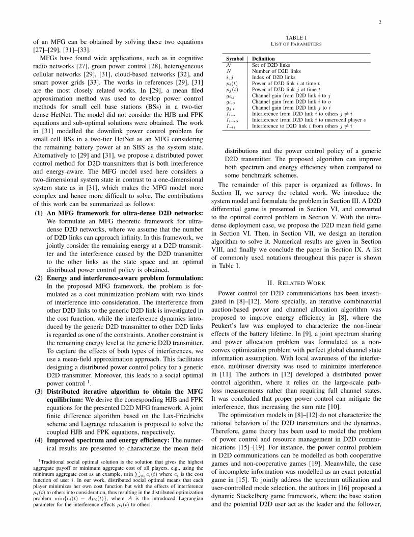
TABLE ILIST OF PARAMETERS

Symbol DefinitionN Set of D2D linksN Number of D2D linksi, j Index of D2D linkspi(t) Power of D2D link i at time tpj(t) Power of D2D link j at time tgi,j Channel gain from D2D link i to jgi,o Channel gain from D2D link i to ogj,i Channel gain from D2D link j to iIi→ Interference from D2D link i to others j 6= iIi→o Interference from D2D link i to macrocell player oI→i Interference to D2D link i from others j 6= i

distributions and the power control policy of a genericD2D transmitter. The proposed algorithm can improveboth spectrum and energy efficiency when compared tosome benchmark schemes.

The remainder of this paper is organized as follows. InSection II, we survey the related work. We introduce thesystem model and formulate the problem in Section III. A D2Ddifferential game is presented in Section VI, and convertedto the optimal control problem in Section V. With the ultra-dense deployment case, we propose the D2D mean field gamein Section VI. Then, in Section VII, we design an iterationalgorithm to solve it. Numerical results are given in SectionVIII, and finally we conclude the paper in Section IX. A listof commonly used notations throughout this paper is shownin Table I.

II. RELATED WORK

Power control for D2D communications has been investi-gated in [8]–[12]. More specially, an iterative combinatorialauction-based power and channel allocation algorithm wasproposed to improve energy efficiency in [8], where thePeukert’s law was employed to characterize the non-lineareffects of the battery lifetime. In [9], a joint spectrum sharingand power allocation problem was formulated as a non-convex optimization problem with perfect global channel stateinformation assumption. With local awareness of the interfer-ence, multiuser diversity was used to minimize interferencein [11]. The authors in [12] developed a distributed powercontrol algorithm, where it relies on the large-scale path-loss measurements rather than requiring full channel states.It was concluded that proper power control can mitigate theinterference, thus increasing the sum rate [10].

The optimization models in [8]–[12] do not characterize therational behaviors of the D2D transmitters and the dynamics.Therefore, game theory has been used to model the problemof power control and resource management in D2D commu-nications [15]–[19]. For instance, the power control problemin D2D communications can be modelled as both cooperativegames and non-cooperative games [19]. Meanwhile, the caseof incomplete information was modelled as an exact potentialgame in [15]. To jointly address the spectrum utilization anduser-controlled mode selection, the authors in [16] proposed adynamic Stackelberg game framework, where the base stationand the potential D2D user act as the leader and the follower,

3

respectively. The authors in [17] investigated a repeated gametheoretic resource allocation, where a D2D link was located inthe overlapping area of two neighboring cells. In [18], a de-centralized framework of joint spectrum allocation and powercontrol was proposed to coordinate interference between theD2D layer and the cellular layer.

The authors in [20] formed D2D clusters using the dis-tributed merge-and-split algorithm from the coalition gametheory and defined a relaxation factor to give a constrainton total energy consumption for each cluster. In [21], twotypes of games were considered including the non-cooperativeStackelberg and the cooperative Nash bargaining game. Theauthors in [22] introduced a spectrum sharing model for D2Dlinks which was analyzed by using a Bayesian non-transferableutility overlapping coalition formation game model. The au-thors in [23] developed a hierarchical framework based on alayered coalitional game for operator-controlled D2D networkswith multiple D2D operators at the upper layer and a groupof devices at the lower layer.

In summary, both non-cooperative and cooperative gameshave been widely used to derive distributed resource allocationtechniques. For example, potential games [15], Stackelberggames [16], repeated games [17], pricing-based games [18]have found extensive applications. On the other hand, coop-erative games in [19], [20], Bayesian overlapping coalitiongames [22], the layered coalition games [23], and Nashbargaining cooperative games [21] are cooperative games. Ashas been mentioned before, these conventional games modelthe interaction of each player with every other player; however,the analysis of a system with a large number of players(e.g., an ultra-dense D2D network) can be complex with thesetraditional game models.

III. SYSTEM MODEL AND PROBLEM FORMULATION

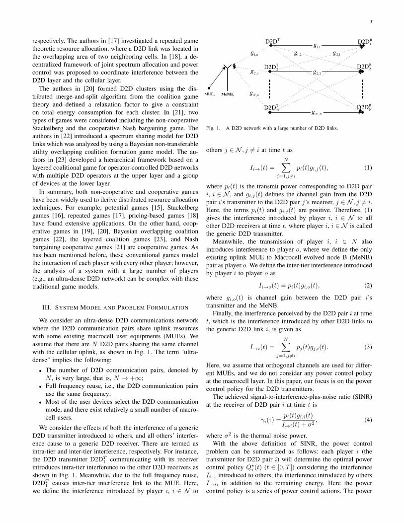
We consider an ultra-dense D2D communications networkwhere the D2D communication pairs share uplink resourceswith some existing macrocell user equipments (MUEs). Weassume that there are N D2D pairs sharing the same channelwith the cellular uplink, as shown in Fig. 1. The term "ultra-dense" implies the following:

• The number of D2D communication pairs, denoted byN , is very large, that is, N → +∞;

• Full frequency reuse, i.e., the D2D communication pairsuse the same frequency;

• Most of the user devices select the D2D communicationmode, and there exist relatively a small number of macro-cell users.

We consider the effects of both the interference of a genericD2D transmitter introduced to others, and all others’ interfer-ence cause to a generic D2D receiver. There are termed asintra-tier and inter-tier interference, respectively. For instance,the D2D transmitter D2DT1 communicating with its receiverintroduces intra-tier interference to the other D2D receivers asshown in Fig. 1. Meanwhile, due to the full frequency reuse,D2DT1 causes inter-tier interference link to the MUE. Here,we define the interference introduced by player i, i ∈ N to

0H1%R

7�'�' 5

�'�'

7�'�' 5

�'�'

71'�' 5

1'�'

���J

���J

���J ���J

08(R

��RJ

��RJ

�1 RJ

�1 1J

Fig. 1. A D2D network with a large number of D2D links.

others j ∈ N , j 6= i at time t as

Ii→(t) =

N∑j=1,j 6=i

pi(t)gi,j(t), (1)

where pi(t) is the transmit power corresponding to D2D pairi, i ∈ N , and gi,j(t) defines the channel gain from the D2Dpair i’s transmitter to the D2D pair j’s receiver, j ∈ N , j 6= i.Here, the terms pi(t) and gi,j(t) are positive. Therefore, (1)gives the interference introduced by player i, i ∈ N to allother D2D receivers at time t, where player i, i ∈ N is calledthe generic D2D transmitter.

Meanwhile, the transmission of player i, i ∈ N alsointroduces interference to player o, where we define the onlyexisting uplink MUE to Macrocell evolved node B (MeNB)pair as player o. We define the inter-tier interference introducedby player i to player o as

Ii→o(t) = pi(t)gi,o(t), (2)

where gi,o(t) is channel gain between the D2D pair i’stransmitter and the MeNB.

Finally, the interference perceived by the D2D pair i at timet, which is the interference introduced by other D2D links tothe generic D2D link i, is given as

I→i(t) =

N∑j=1,j 6=i

pj(t)gj,i(t). (3)

Here, we assume that orthogonal channels are used for differ-ent MUEs, and we do not consider any power control policyat the macrocell layer. In this paper, our focus is on the powercontrol policy for the D2D transmitters.

The achieved signal-to-interference-plus-noise ratio (SINR)at the receiver of D2D pair i at time t is

γi(t) =pi(t)gi,i(t)

I→i(t) + σ2, (4)

where σ2 is the thermal noise power.With the above definition of SINR, the power control

problem can be summarized as follows: each player i (thetransmitter for D2D pair i) will determine the optimal powercontrol policy Q?i (t) (t ∈ [0, T ]) considering the interferenceIi→ introduced to others, the interference introduced by othersI→i, in addition to the remaining energy. Here the powercontrol policy is a series of power control actions. The power

4

control problem can be formulated as a differential game dueto the interference dynamics and the energy dynamics [24]–[29]. Different from the studies in [24]–[29], we formulatea power control differential game with two-dimensional statespace and a new cost function.

IV. DIFFERENTIAL GAME MODEL FOR POWER CONTROL

The differential game model for power control in the D2Dnetwork described above is defined as follows:

Definition 1: The D2D differential power control gameGs for D2D transmitters is defined by a 5-tuple: Gs =(N , {Pi}i∈N , {Si}i∈N , {Qi}i∈N , {ci}i∈N ), where

• Player set N : N = {1, ..., N} represents the player setof densely-deployed D2D communication pairs. They arerational policy makers in the D2D power control differ-ential game. The number of D2D links N is arbitrarilylarge.

• Set of actions {Pi}i∈N : This is the set of possibletransmit powers. Each transmitter determines the powerpi(t) ∈ {Pi} at any time t ∈ [0, T ] to minimize the costfunction (to be defined later).

• State space {Si}i∈N : We define the state of player ias the combination of the interference introduced by theD2D transmitter i to other D2D links and the remainingenergy at this D2D transmitter. Thus, we have two-dimensional states.

• Control policy {Qi}i∈N : A power control policy is de-noted by Qi(t), with t ∈ [0, T ], to minimize the averagecost over the time interval T with two-dimensional states.

• Cost function {ci}i∈N : We will define a novel cost func-tion, where we consider both the achieved performance,e.g., the SINR at the receiver of a generic D2D link andthe transmit power.

To determine the control policy {Qi}i∈N , we need to definethe state space {Si}i∈N and the cost function {ci}i∈N .

A. Two-Dimensional State Space

The state space is defined based on the intra-tier and inter-tier interferences in (1) and (2), respectively, and the energyusage dynamics.

1) Energy Usage Dynamics: The remaining energy stateEi(t) of the player i at time t is equal to the amount ofavailable energy. Meanwhile, 0 ≤ Ei(t) ≤ Ei(0), whereEi(0) is the energy at time 0. The power control at time tshould be any pi(t) ∈ [0, pmax], where pmax is the maximumpossible transmit power. Without loss of generality, we definethe evolution law of the remaining energy in the battery as

dEi(t) = −pi(t)dt, (5)

which means that energy Ei(t) of the battery deceases withthe transmit power consumption pi(t). At the same time, ingame Gs, each player i should also consider the impact ofinterference on others.

2) Interference Dynamics: With intra-tier and inter-tierinterference defined in (1) and (2), respectively, we first definethe interference function that describes the interference causedby the generic D2D transmitter to others as follows:

µi(t) = Ii→(t) + Ii→o(t), (6)

where (6) describes all the interference introduced by playeri to other D2D pairs j ∈ N , j 6= i and the only MUE o.According to definitions in (1) and (2), we have

µi(t) =

N∑j=1,j 6=i

pi(t)gi,j(t) + pi(t)gi,o(t). (7)

To simplify the notation, we represent (7) as

µi(t) = pi(t)εi(t), (8)

where εi(t) =N∑

j=1,j 6=igi,j(t) + gi,o(t). From (8), the total

interference at time t to others depends on pi(t) and εi(t) attime t. Therefore, we can define the interference state as

dµi(t) = εi(t)dpi(t) + pi(t)∂tεi(t). (9)

We will introduce the mean field approximation method toestimate the channel gains εi, i ∈ N in the following section.

We define the following state space for player i:

si(t) = [Ei(t), µi(t)] , i ∈ N , (10)

where the interference caused by the generic D2D transmitterto other D2D links is regarded as one of the state variables.

The interference state µi(t) in (9) of the generic D2Dtransmitter will affect the strategy of the players of the MeNBand the other D2D receivers, and all others’ interferenceI→i(t) introduced to the generic receiver will affect the SINRperformance. To distinguish between these two interferences,we denote them as State1 (which is one of the state vari-ables) and State2, respectively. Note that the formulated costminimization problem considers both SINR performance andcost due to transmit power. While the former is related tothe interference caused to the generic D2D receiver from allthe other transmitters, the latter is related to the interferencecaused by the generic D2D transmitter to others (i.e., theobjective function of player i implicitly captures the effectsof µi). Therefore, the objective function is affected by theconsidered interference states.

B. Cost Function

With the above definition of state space si(t), each D2Dtransmitter i will determine the optimal power control policyQ?i (t), with t ∈ [0, T ] to minimize the cost. The commu-nication performance of the D2D pair i is characterized bythe SINR γi(t) defined in (4). We assume an identical SINRthreshold γth for all D2D communication pairs. Meanwhile,each D2D communication pair prefers to minimizing thepower consumption, and finally the cost function is given by

ci(t) =(γi(t)− γth(t)

)2+ λpi(t), (11)

where λ is introduced to balance the units of the achievedSINR difference and the consumed power. It is easy to prove

5

that the cost function ci(t), given by (11) is convex withrespect to pi(t).

V. OPTIMAL CONTROL PROBLEM AND ANALYSIS

With the cost function including both the achieved perfor-mance and transmit power, the problem is formulated as thecost minimization problem taking two kinds of interferencesand the remaining energy into consideration.

A. Optimal Control Problem

We consider the problem that each D2D pair i will deter-mine the optimal power control policy Q?i (t), with t ∈ [0, T ]to minimize the cost function ci(t), given by (10), during afinite time horizon [0, T ]. The general optimal control problemcan be stated as follows:

Q?i (t) = arg minpi(t)

E

[∫ T

0

ci(t)dt+ ci(T )

], (12)

where ci(T ) is the cost at time T . At this time, we define thevalue function as follows:

ui(t, si(t)) = minpi(t)

E

[∫ T

t

ci(t)dt+ ui(T, si(T ))

], t ∈ [0, T ] ,

(13)where ui(T, si(T )) is a value at the final state si(T ) attime T . With the defined two-dimensional states, we have thefollowing lemma 1.

Lemma 1: A power control profile Q?i (t) = p?i (t), for i ∈N is the Nash equilibrium solution of Gs if and only if [31]

Q?i (t) = arg minpi(t)

E

[∫ T

0

ci(pi(t), p?−i)dt+ ci(T )

]

subject to:

si(t) = [µi(t), Ei(t)] ,

dEi(t) = −pi(t)dt, and

dµi(t) = εi(t)dpi(t) + pi(t)∂tεi(t),

where p?−i denotes the transmit power vector of D2D linksexcept D2Di. None of the players can have a lower cost byunilaterally deviating from the current power control policy.The Nash equilibrium of the above power control differentialgame can be obtained by solving the HJB equation associatedwith each player in the optimal control theory. We will derivethe HJB equation later.

Proof: The conclusion is indirectly guaranteed by thesmoothness of the HJB function. Therefore, we first derivethe HJB equation, and then we prove that the smoothness ofthe derived HJB equation guarantees the existence of Nashequilibrium in the formulated differential game. The detailscan be found in Lemma 2 and Theorem 1 presented below.

B. Analysis

According to optimal control theory followed by Bellman’soptimality principle [26], the value function in (13) shouldsatisfy a partial differential equation which is a HJB equation.The solution of the HJB equation is the value function, whichgives the minimum cost for a given dynamic system with anassociated cost function.

Lemma 2: We have the HJB equation in (14)

−∂tui(t, si(t)) = minpi(t)

[ci(t, si(t), pi(t)) + ∂tsi(t) · ∇ui(t, si(t))] ,(14)

where we define the Hamiltonian as in (15).Proof: Proof of Lemma 2 is given in Appendix A.

The Nash equilibrium of the above differential game canbe obtained by solving the HJB equation associated witheach player given in (37). We have following theorem on theexistence of the Nash equilibrium for the defined Gs in thedefinition 1.

Theorem 1: There exists at least one Nash equilibrium forthe differential game Gs.

Proof: Existence of a solution to the HJB equationensures the existence of the Nash equilibrium for the gameGs. It is known that there exists a solution to the HJB equationif the Hamiltonian is smooth [31]. Derivatives of all the ordersexist for the Hamiltonian due to the continuity of the definedcost function, and it is easy to derive the derivatives of theHamiltonian with respect to pi(t). Due to the existence ofthe derivatives, the Hamiltonian is smooth. This concludes theproof.

Obtaining the equilibrium for game Gs for a system withN players involves solving N partial differential equationssimultaneously. However, for a dense D2D network, it is notpossible to obtain the Nash equilibrium in this manner due tothe large number of simultaneous partial differential equations.Therefore, for modeling and analysis of a dense D2D network,a mean field game will be introduced where the system can bedefined solely by two coupled equations. In the next section,we show the extension of game Gs to a mean field game.

VI. MEAN FIELD GAME (MFG) FOR POWER CONTROL

The power control MFG in D2D networks is a special formof a differential game described before when the number ofD2D links approaches infinity. The power control MFG can beexpressed as a coupled system of two equations of HJB andFPK. On one hand, an FPK type equation evolves forwardin time that governs the evolution of the density function ofthe agents. On the other hand, an HJB type equation evolvesbackward in time that governs the computation of the optimalpath for each agent.

A. Mean Field and Mean Field Approximation

For the effects of both the interference of the generic D2Dtransmitter introduced to others, and all others’ interferenceintroduced to the generic link, we first introduce the meanfield concept, and then propose the mean-field approximationapproach.

6

H(pi(t), si(t),∇ui(t, si(t))) = minpi(t)

[ci(t, si(t), pi(t)) + ∂tsi(t) · ∇ui(t, si(t))] . (15)

1) Mean Field: This is a critical concept in the definedpower control MFG, which is a statistical distribution of thedefined two-dimensional states.

Definition 2: Given the state space si(t) = [µi(t), Ei(t)]in the defined power control MFG, we define the mean fieldm(t, s) as

m(t, s) = limN→∞

1

N

N∑i=1

1{si(t)=s}, (16)

where 1 denotes an indicator function which returns 1 if thegiven condition is true and zero, otherwise. For a given timeinstant, the mean field is the probability distribution of thestates over the set of players.

With the defined mean field, the power control differentialgame can be formulated as the new power control MFG, ifthe following requirements are satisfied. In the context of anultra-dense D2D network, the D2D transmitters, which act asplayers, have the following properties:• Rationality: Each D2D transmitter can individually take

rational power control decision to minimize the costfunction.

• The existence of a continuum of the players (i.e.,continuity of the mean field): The presence of a largenumber of D2D pairs in the defined power control gameensures the existence of the continuum of the players.

• Interchangeability of the states among the players (i.e.,permutation of the states among the players wouldnot affect the outcome of the game): We derive the costfunction via mean-field approximation of the interferencein order to ensure the interchangeability of the actionsamong the players.

• Interaction of the players with the mean field: EachD2D player interacts with the mean field instead ofinteracting with all the other players.

The mean field defined above will be obtained based onmean field approximation described below.

2) Mean Field Approximation: With respect to the inter-ference summations Ii→(t) and I→i(t) defined in (1) and (3),respectively, we assume that each interferer is infinitesimal andcontributes little interference power to the summation. Theinfinite mass of other players, which is called as the mean-field value, dominates the interference effects when studyinga typical player. We first derive the interference mean field viaa special technique of the mean field approximation [29]. Forboth State1 Ii→(t) and State2 I→i(t) defined in (1) and (3),we can use the same method. Here, we use State2 I→i(t) asan example. We know that

I→i(t) =

N∑j=1,j 6=i

pj(t)gj,i(t) ≈ (N − 1) pj(t)gj,i(t), (17)

where pi(t) is the known test transmit power and we assumethat all the players involved in the game are using the same test

transmit power. The term gi,j(t) defines the mean interferencechannel gain of ultra-dense infinitesimal D2D effects, whichcan be estimated by the following idea. If we use pi(t) at thetransmit power for D2D pair i’s transmitter, then the powerreceived at the corresponding receiver is

pRi (t) = pi(t)gi,i(t) + I→i(t), (18)

where gi,i(t) is the effective channel gain, and pi(t)gi,i(t)is the effective received power, and I→i(t) is the receivedinterference power from all the others.

Combining (17) and (18), we can derive the only unknownvariable gj,i(t) as

pRi (t) = pi(t)gi,i(t) + (N − 1) pj(t)gj,i(t), (19)

and we have

gj,i(t) =pRi (t)− pi(t)gi,i(t)

(N − 1) pj(t). (20)

With the above mean field approximation,

γi(t) =pi(t)gi,i(t)

(N − 1) pj(t)gj,i(t) + σ2, (21)

with gj,i(t) estimated by the above method during the practicalimplementation. The mean field cost function is then definedas

ci(t) =(γi(t)− γth(t)

)2+ λpi(t). (22)

In the following sections, we will use the mean field costfunction and the approximated interference mean field. Wecan similarly achieve the mean field approximation of State1Ii→(t).

B. Mean Field Game

Based on the above definition of mean field and mean fieldapproximation, we derive the FPK equation first.

Lemma 3: The FPK equation of the defined MFG is givenby

∂tm(t, s) +∇ (m(t, s) · ∂ts(t)) = 0, (23)

where s is the state.Proof: Proof of Lemma 3 can be found in [24].

The FPK equation describes the evolution of the definedmean field with respect to time and space. At this time, withthe derived HJB and FPK equations, we formulate the D2DMFG as follows.

Definition 3: The D2D MFG is defined as the combinationof derived HJB and FPK equations, where the HJB equationis

−∂tu(t, s(t)) = minp(t)

[c(t, s(t), p(t)) + ∂ts(t) · ∇u(t, s(t))] ,

(24)and the FPK equation is in (23).

Their interactions with each other are shown in Fig. 2.The HJB equation governs the computation of the optimal

7

���

���

� � � � � � � � � �

Fig. 2. D2D mean field game with HJB and FPK equations.

control path of the player, while the FPK equation governs theevolution of the mean field function of players. Here, the HJBand FPK equations are termed as the backward and forwardfunctions, respectively. Backward means that the final valueof the function is known, and we determine the value of u(t)at time [0, T ]. Therefore, the HJB equation is always solvedbackwards in time, starting from t = T , and ending at t = 0.When solved over the the entire state space, the HJB equationis a necessary and sufficient condition for the optimum. TheFPK equation evolves forward with time. The interactiveevolution finally leads to the mean field equilibrium.

C. Mean Field Equilibrium

We define the mean field equilibrium, which can be achievedby using the finite difference method [31].

Definition 4: Mean field equilibrium (MFE) represents sta-ble combination of both the control policy u?(t, s) and themean field m?(t, s) at any time t and state s in Fig. 2.

At any time t and state s, the control policy u(t, s) and themean field m(t, s) interact with each other, where u(t, s) isalso termed as the value function. The value function u(t, s)determines the control policy Q(t, s). The term u(t, s) isthe solution of the HJB equation in (24) and m(t, s) is thesolution of the FPK equation in (23). The term u(t, s) affectsthe evolution of the mean field, and m(t, s) determines thedecision-making of optimal policy u(t, s).

VII. DISTRIBUTED SOCIAL-OPTIMAL POWER CONTROLPOLICY BASED ON THE FINITE DIFFERENCE METHOD

Similar to [31], we resort to the finite difference method.We have three different schemes to discretize the advectionequation including Upwind, Lax-Friedrichs, and Lax-Wendroff[30] schemes. Different schemes have different rates of con-vergence. We select the Lax-Friedrichs scheme to guaranteethe positivity of the mean field with first-order accuracy inboth time and space [31].

In the framework of the finite difference method, the investi-gated time interval [0, T ], the energy state space [0, Emax], andthe interference state space [0, µmax] should be discretized intoX×Y ×Z spaces, as shown in Fig. 3. In Fig. 3, we illustratethree curves in the three-dimensional discretized time andspace. The optimal control policy covers the decision-makingover a period in the discretized mean field game framework.

�

�

�

��� ���� � � �� � �

�������

����������������

Fig. 3. Optimal control of the discretized mean field game in time and space,where there exist several potential control paths. Here, we should design themethod to find the optimal control path.

Therefore, there exist several potential control paths. Here, weshould design the method to find the optimal control path asindicated in the figure. Thus, we first define the iteration stepsof time, energy, and interference spaces as

δt =T

X, δE =

Emax

Y, δµ =

µmax

Z.

Therefore, the FPK equation will evolve in the space ofthree dimensions of (0, T ) × (0, Emax) × (0, µmax) with thesteps of δt, δE , and δµ, respectively. At the same time, theoptimal control path is achieved by solving the HJB equa-tion backward accordingly. A joint finite difference algorithmis then developed based on the Lax-Friedrichs scheme andLagrange relaxation to solve the corresponding coupled HJBand FPK equations to obtain the optimal power control policy(e.g., the optimal control path as shown in Fig. 3).

A. Lax-Friedrichs Scheme to Solve FPK Equation

We solve the FPK equation using the Lax-Friedrichsmethod, where we first solve the FPK equation

∂tm(t, s) +∇Em(t, s)E(t) +∇µm(t, s)µ(t) = 0. (25)

By applying the Lax-Friedrichs scheme, we have (26).Here M(i, j, k), P (i, j, k), ε(i, j, k) are the values of the

mean field, the power, and the interference gain at time instanti with the energy level j and the interference state k in thediscretized grid.

B. Discretized Lagrange Relaxation to HJB

The finite difference method cannot be used to solve theHJB equation due to the Hamiltonian. Here, we reformulatethe HJB equation using its corresponding optimal controlproblem, where the newly-defined problem is

minpi(t)

E[∫ T

0ci(t)dt+ ci(T )

],

subject to : ∂tm(t, s) +∇Em(t, s)E(t) +∇µm(t, s)µ(t) = 0.

(27)

8

M (i+ 1, j, k) =1

2[M (i, j − 1, k) +M (i, j + 1, k) +M (i, j, k − 1) +M (i, j, k + 1)]

+δt

2δE[M (i, j + 1, k)P (i, j + 1, k)−M (i, j − 1, k)P (i, j − 1, k)]

+δt

2δµ[M (i, j, k + 1)P (i, j, k + 1) ε (i, j, k + 1)−M (i, j, k − 1) ε (i, j, k − 1)P (i, j, k − 1)] ,

(26)

L (m(t, s), p(t, s), λ(t, s))

= E

[∫ T

0

ci(t)dt+ ci(T )

]+

T∫t=0

Emax∫E=0

µmax∫µ=0

λ(t, s) (∂tm(t, s) +∇Em(t, s)E(t) +∇µm(t, s)µ(t)) dtdEdµ

=

T∫t=0

Emax∫E=0

µmax∫µ=0

[c(t, s)m(t, s) + λ(t, s) (∂tm(t, s) +∇Em(t, s)E(t) +∇µm(t, s)µ(t))] dtdEdµ.

(28)

At this time, we obtain the LagrangianL (m(t, s), p(t, s), λ(t, s)) by introducing a Lagrangemultiplier λ(t, s) as (28), where we assume that c(T ) = 0.

Similar to the method to solve the FPK equation, wepropose a finite difference method to solve (28). We firstdiscretize the Lagrangian to solve the newly-defined optimalcontrol problem, and the discretized Lagrangian is given by(29). Here Υ, Φ, and Ψ are given by (30), (31), and (32),respectively.

Here, M(i, j, k), P (i, j, k), λ(i, j, k), and C(i, j, k) are thevalues of the mean field, the power, Lagrange multiplier, andcost function at time instant i, energy level j, and interferencestate k in the discretized grid.

The optimal decision variables include P ?, M?, and λ?.We derive the optimal power control as ∂Ld

∂P (i,j,k) = 0 for anyarbitrary point (i, j, k) in the discretized grid, where ∂Ld

∂P (i,j,k)is given by (33).

Furthermore, for any arbitrary point (i, j, k) in the dis-cretized grid, we update the Lagrange multiplier λ(i, j, k) bycalculating ∂Ld

∂M(i,j,k) = 0, and then we have λ (i− 1, j, k)given by (34).

C. Distributed Social-Optimal Power Control Policy

Following the above derivations, a joint finite differencealgorithm based on the Lax-Friedrichs scheme and Lagrangerelaxation is proposed to solve the coupled HJB and FPKequations, respectively. We name it as the distributed social-optimal power control policy.

For the proposed distributed algorithm, we have the follow-ing comments:

• First, the mean filed is jointly influenced by the energydynamics and interference dynamics (State1). Basically,the energy dynamic function is a linear function withrespect to the transmit power. However, interferencefunction is not linear. At each time step, we assume thatthe interfering link gains estimated by the mean fieldapproximation approach do not change.

Algorithm 1: Distributed social-optimal power controlpolicy

1 Initialization:2 M(0, 0, 0):= joint mean field distribution;3 λ(X + 1, 0, 0):= initial Lagrangian parameters;4 P (X + 1, 0, 0):= initial power levels.5 for i = 1 : X , j = 1 : Y , and k = 1 : Z do6 Update mean field:7 Using M(i+ 1, j, k) (26)8 if P(i,j+1,k)=0 then9 M(i+ 1, j + 1, k + 1) = M(i, j, k)

10 else11 M(i+ 1, j + 1, k + 1) = 012 end13 Update Lagrangian parameter:14 λ(i− 1, j, k) using (34)15 Update power levels:16 P (i− 1, j, k) using (33)17 end

• Second, we choose the algorithm termination conditionas the difference between the final-two mean field values,and we set the gap as 10−5.

• Third, during iterations i − 1 and i + 1 and similarlyfor other indices in the proposed algorithm, we introducea simple computation method. For instance, i − 1 maynot be positive, when i ≤ 1. In this situation, we setλ(i− 1, j, k) = 1

2 [λ(i, j + 1, k) + λ(i, j − 1, k)].• Our algorithm jointly considers the Emax and the toler-

able interference µmax2. Therefore, it is easy to extend

as the other schemes, for instance, it can be termed asthe ’blind’ scheme when Emax → +∞ and µmax → 0.For the cases of µmax → 0 and Emax → +∞, wemake the following assumptions during simulations. Weassume that if the maximum energy is set more than ten

2Tolerable interference µmax is a predefined value, which constrains thetotal interference power that can be tolerated.

9

Ld = δtδEδµ

X+1∑i=1

Y+1∑j=1

Z+1∑k=1

[M (i, j, k)C (i, j, k) + λ(i, j, k)(Υ + Φ + Ψ)

], (29)

Υ =1

δt

[M (i+ 1, j, k)− 1

2(M (i, j + 1, k) +M (i, j − 1, k) +M (i, j, k + 1) +M (i, j, k − 1))

], (30)

Φ =1

2δµ[M (i, j, k + 1)P (i, j, k + 1) ε (i, j, k + 1)−M (i, j, k − 1)P (i, j, k − 1) ε (i, j, k − 1)] , (31)

Ψ =1

2δE[M (i, j + 1, k)P (i, j + 1, k)−M (i, j − 1, k)P (i, j − 1, k)] . (32)

times higher than that of practical situation, then it can beregarded as the case of Emax → +∞. While the normalsetting is Emax = 0.5, the case of Emax = 5 can be seenas the case of Emax → +∞.

VIII. NUMERICAL RESULTS

In this section, we first illustrate the simulation scenariosand the basic settings with relevant simulation parameters. Wecharacterize the mean field distributions and the power controlpolicy using the Matlab software.

A. Basic Simulation Settings

The downlink transmission of an OFDMA D2D network,with the radius of D2D links uniformly distributed between10 m to 30 m is considered. We set the system parametersas the bandwidth w = 20 MHz, and background noise poweris 2 × 10−9 W as the noise power spectral density is κ =-174 dBm/Hz. Without special instructions, we choose thestandardized case with 500 LTE frames, the maximum energyis 0.5 J, the number of D2D links will vary from N = 50 to N= 200. The path-loss exponent for D2D links is 3. The durationof one LTE radio frame is 10 ms, and for 500 frames, T = 5s. We also pick, Emax to be 0.5 J. The tolerable interferencelevel of each player µmax is assumed to be 5.8× 10−6 W.

B. Characteristics of Mean Field Distributions and PowerControl Policy

To illustrate the properties of our proposed power controlscheme, we show the distributions of the mean field and thepower control policy in different cases.

First, we describe three dimensional mean field distributionsand power policy, as shown in Fig. 4. However, mean field andpower policy are four dimensional vectors. Therefore, we plotmean field and power policy for three cases, i.e., (a) meanfield distributions with varying interference and energy butfixed time; (b) mean field distributions with varying time andenergy but fixed interference; and (c) mean field distributionswith varying time and interference but fixed energy. Similarly,we illustrate the power control policies for these three cases.Basically, we can see that both the remaining energy and the

interference dynamics affect the mean field distributions andpower control policy.

Second, to further demonstrate the properties of our pro-posed scheme, the cross sections of mean field distributionsand power policy at the energy states after convergence butwith varying times are depicted in Fig. 5. Here, as in theprevious settings, we discretize the time interval, the energyspace, and the interference space into 20× 20× 20 grids. Toreflect the reasons why the mean field distributions and powerpolicy in Fig. 4 are random, we describe Fig. 5, where wefirst show the distributions of the mean field with respect tothe interference space at the energy states after convergence.In addition, we select three cases: (a) distributions of meanfield with respect to the varying interference at time interval13; (b) distributions of mean field with respect to the varyinginterference at time interval 15; and (c) distributions of meanfield with respect to the varying interference at time interval20. Meanwhile, we depict the distributions of power policyaccordingly in (d), (e), and (f), respectively.

From Fig. 5, we have the following observations. On onehand, the randomness of the distributions of mean fields andpowers are introduced by the random interference space. Onthe other hand, our proposed scheme can achieve the powerequilibrium as shown in Fig. 5, which is the final powercontrol policy at the final energy and time interval states afterconvergence. Also, our proposed scheme can always achievethe equilibrium powers, regardless of the interference states.

In Fig. 6, we illustrate the mean field distributions and powercontrol policy with respect to time toward the convergence.We can see that we can always achieve the target SINR withthe varying power control policy according to the mean fielddistributions.

C. Spectrum and Energy Efficiency Performance

• Spectrum efficiency: The average spectrum efficiencyπaverage is in the unit of bps/Hz, which is calculated by

πaverage = log2

(1 +

p

I + w × κ

),

where κ is the noise power density and w is the totalbandwidth.

10

∂Ld∂P (i, j, k)

=

Y+1∑j=1

Z+1∑k=1

M (i, j, k)∂C (i, j, k)

∂P (i, j, k)

+

[M (i, j, k)

2δE+M(i, j, k)ε(i, j, k)

2δµ

][λ (i, j + 1, k)− λ (i, j − 1, k)] .

(33)

λ (i− 1, j, k) =1

2[λ (i, j + 1, k) + λ (i, j − 1, k)] +

1

2[λ (i, j, k + 1) + λ (i, j, k + 1)]

− 1

2δtP (i, j, k)

[ε (i, j, k)

δµ+

1

δE

][λ (i, j + 1, k)− λ (i, j − 1, k)]

+ δtC (i, j, k) .

(34)

Fig. 4. Three dimensional mean field distributions and power policy varying in time and space. For the distributions of mean field we have three cases with(a) T = 5; (b) µmax = 5.8× 10−6; (c) Emax = 0.1 fixed, respectively. Similarly, for the distributions of powers we also have three cases with (d) T = 5;(e) µmax = 5.8× 10−6; and (f) Emax = 0.1, respectively.

• Energy efficiency: The average energy efficiency ηaverageis defined as the ratio between the total throughput andthe consumed energy, which is given by

ηaverage =wπaverage

ptotal,

which is in the unit of bit/J.

To illustrate the impacts of various interference constraints,we simulate two other cases as benchmarks of the normalsettings in our work: (1) µmax → +∞, which means thatthe interference tolerance is very large; (2) µmax → 0, which

means that the interference tolerance is very small. Meanwhile,to illustrate the impacts of various energy constraints, inaddition to the normal settings, we simulate the case ofEmax → +∞, which means that the battery is always fullypowered.

We set µmax = 5.8×10−6 as the normal setting. Moreover,the case µmax ≤ 10−5× normal setting is considered as thecase of µmax → 0. The case µmax ≥ 102× normal settingis considered as the case of µmax → +∞. Here, we set thenormal setting is Emax = 0.5, while the case of Emax = 5can be seen as the case of Emax → +∞.

11

� �� �� ���

���

���

���

���

���

��� �������������

������� ��

� �� �� ���

����

���

����

���

����

���

����

��� �������������

������� ��

� �� �� ���

���

���

���

���

���

��� �������������

������� ��

� �� �� ���

����

����

����

����

���

��� �������������

������� ������

� �� �� ���

���

���

���

���

��� �������������

������� ������

� �� �� ���

����

����

����

����

����

��� ����������� �

������� ������

Fig. 5. Cross sections of mean field distributions and power policy at thestates after convergence but with varying times. For the distributions of meanfield we have three cases at different time slots (a) T = 3.25s; (b) T = 3.75s;(c) T = 5s, respectively. Similarly, for the distributions of powers we alsohave three cases with at different time slots (d) T = 3.25s; (e) T = 3.75s;(f) T = 5s, respectively.

� � �� �� �� ������

�

���

�

����

�

� � �� �� �� ���

����

���

����

����

� � �� �� �� ���

����

����

����

����

����

Fig. 6. Cross-sections of mean field distributions and power policy at theinterference µmax = 5.8 × 10−6 and energy state Emax = 0.5J afterconvergence.

We illustrate the spectrum efficiency π performance of thetwo cases in Fig. 7(a) and Fig. 7(b), respectively. We observethat:• The spectrum efficiency decreases with the increasing

numbers of the D2D links. This is due to the increasedmutual interference with increasing number of D2D links.

• Minimizing the tolerable interference can always improvethe spectrum efficiency; however, maximizing the avail-able energy, i.e., Emax does not always improve thespectrum efficiency. Minimizing the tolerable interferencemeans that the power used at each state is not allowed tobe too large, which leads to the reduced SINR. Thus,maximizing the tolerable interference means that the

Fig. 7. Spectrum efficiency, which is measured in the unit of bps/Hz.

Fig. 8. Energy efficiency, which is measured in the unit of b/J.

power used at each state can be large, therefore, thespectrum efficiency is improved.

• Maximizing the available energy can first help maximiz-ing the effective received energy; however, at some pointsincreasing the energy also means increasing the inter-ference power, and consequently, decreases the spectrumefficiency.

In Fig. 8, we illustrate the improved energy efficiencyperformance of the proposed interference and energy-awarepower control compared to the blind power control scheme.Here, we term the blind power control scheme as the caseof Emax → +∞, which can be seen as the scheme withoutthe energy constraint. Therefore, D2D transmitter in the blindpower control scheme can individually increase the transmis-sion power, which will both introduce the interference to othersand exhaust the battery soon.

It can be concluded from Fig. 8 that the proposed interfer-ence and energy-aware power control can achieve higher en-ergy efficiency compared with the blind power control scheme.Meanwhile, the benefits decrease with the increasing numberof D2D links, which is mainly because that the increasingnumber of D2D links means introducing more interference,and thus decreases the spectrum efficiency.

12

IX. CONCLUSION

We have investigated the effects of both interference andenergy on the power control in ultra-dense D2D commu-nications. We have formulated a mean filed game theoreticframework with the two-dimensional dynamics states. For theMFG framework, we have derived the coupled HJB and FPKequations. Then, a joint finite difference algorithm has beenused to solve the coupled HJB and FPK equations of thecorresponding MFG, which is based on the Lax-Friedrichsscheme and the Lagrange relaxation method. Then we havedeveloped an interference and energy-aware distributed powercontrol. Numerical results have been presented to characterizethe mean field distributions and the power control policy. Thespectrum and energy efficiency performances of the proposeddistributed power control scheme have been illustrated. Theproposed model can be implemented in practical systems bysolving the MFG model offline using the measured (historical)information about interference dynamics as well as the energyavailability at the terminals in a dense D2D network. Theobtained power control policies can be stored in look-up tablesto be used by the D2D transmitters.

APPENDIX ADERIVATION OF HJB

Intuitively, an HJB can be derived as follows. If ui(t) isthe value function of power pi(t) and the state si(t), and thenby the Richard Bellman’s principle of optimality, increasingtime t to t + dt, we have (35). Further, we compute theTaylor expansion of ui(t + dt), and we have (36). Here ∂tuis the differential function with t, and ∇u is the gradient ofthe function u with s. o(dt) denotes the terms of the Taylorexpansion of higher order than one, and we omit it during thefollowing analysis.

Substituting (36) into (35), and canceling ui(t, si(t)) onboth sides, dividing by dt, and taking the limit with dtapproaches zero, we have the following HJB equation (37).Here, we define the Hamiltonian as (38).

REFERENCES

[1] Z. Zhou, M. Dong, K. Ota, J. Wu, and T. Sato, “Energy efficiency andspectral efficiency tradeoff in device-to-device (D2D) communications,”IEEE Wireless Communications Letters, vol. 3, no. 5, pp. 485–488, Oct.2014.

[2] L. Song, D. Niyato, Z. Han, and E. Hossain, Wireless device-to-devicecommunications and networks, Cambridge University Press, 2015.

[3] Z. Zhou, M. Dong, K. Ota, and Z. Chang, “Energy-efficient context-aware matching for resource allocation in ultra-dense small cells,” IEEEAccess, vol. 3, pp. 1849–1860, Sep. 2015.

[4] N. Bhushan, J. Li, D. Malladi, R. Gilmore, D. Brenner, A. Damnjanovic,R. Sukhavasi, C. Patel, and S. Geirhofer, “Network densification: thedominant theme for wireless evolution into 5G,” IEEE CommunicationsMagazine, vol. 52, no. 2, pp. 82–89, Feb. 2014.

[5] B. Soret, K. Pedersen, Niels T. K. Jrgensen, and F. L. Vctor, “Interfer-ence coordination for dense wireless network,” IEEE CommunicationsMagazine, vol. 53, no. 1, pp. 102–109, Jan. 2015.

[6] H. Zhang, C. Jiang, J. Cheng, and V. C. M. Leung, “Cooperativeinterference mitigation and handover management for heterogeneouscloud small cell networks,” IEEE Wireless Communications, vol. 22,no. 3, pp. 92–99, Jun. 2015.

[7] C. Yang, J. Li, and M. Guizani, “Cooperation for spectral and energyefficiencies in ultra-dense heterogeneous and small cell networks,” IEEEWireless Communication Magazine, vol. 23, no. 1, pp. 64–71, Feb. 2016.

[8] F. Wang, C. Xu, L. Song, and Z. Han, “Energy-efficient resource alloca-tion for device-to-device underlay communication,” IEEE Transactionson Wireless Communications, vol.14, no. 4, pp. 2082–2092, Apr. 2015.

[9] R. Yin, C. Zhong, G. Yu, Z. Zhang, K. K. Wong, and X. Chen, “Jointspectrum and power allocation for D2D communications underlayingcellular networks,” IEEE Transactions on Vehicular Technology, vol.65, no. 4, pp. 2182–2195, Apr. 2016.

[10] C.-H. Yu, O. Tirkkonen, K. Doppler, and C. Ribeiro, “Power optimiza-tion of device-to-device communication underlaying cellular communi-cation,” IEEE International Conference on Communications, pp. 1–5,Jun. 2009.

[11] P. Janis, V. Koivunen, C. Ribeiro, J. Korhonen, K. Doppler, andK. Hugl, “Interference-aware resource allocation for device-to-deviceradio underlaying cellular networks,” IEEE 69th Vehicular TechnologyConference, Barcelona, Spain, Apr. 2009.

[12] G. Fodor and N. Reider, “A distributed power control scheme forcellular network assisted D2D communications,” 2011 IEEE GlobalTelecommunications Conference (GLOBECOM 2011), Houston TX,Dec. 2011.

[13] P. Phunchongharn, E. Hossain, and D. I. Kim, “Resource allocation fordevice-to-device communications underlaying LTE-advanced networks,”IEEE Wireless Communication Magazine, vol. 20, no. 4, pp. 91–100,Aug. 2013.

[14] Z. Zhou, M. Dong, K. Ota, G. Wang and L. T. Yang, “Energy-efficientresource allocation for D2D communications underlaying cloud-RAN-based LTE-A networks,” IEEE Internet of Things Journal, vol. 3, no. 3,pp. 428–438, June 2016.

[15] S. Maghsudi and S. Stanczak, “Hybrid centralized-distributed resourceallocation for device-to-device communication underlaying cellular net-works,” IEEE Transactions on Vehicular Technology, vol. 65, no. 4, pp.2481–2495, April 2016.

[16] K. Zhu and E. Hossain, “Joint mode selection and spectrum partitioningfor device-to-device communication: a dynamic Stackelberg game,”IEEE Transactions on Wireless Communications, vol. 14, no. 3, pp.1406–1420, Mar. 2015.

[17] J. Huang, Y. Zhao, and K. Sohraby, “A game-theoretic resource alloca-tion approach for intercell device-to-device communications in cellularnetworks,” 23rd International Conference on Computer Communicationand Networks (ICCCN), Shanghai, China, Aug. 2014.

[18] R. Yin, G. Yu, H. Zhang, Z. Zhang, and G. Y. Li, “Pricing-based interfer-ence coordination for D2D communications in cellular networks,” IEEETransactions on Wireless Communications, vol. 14, no. 3 pp. 1519–1532,Mar. 2015.

[19] L. Song, D. Niyato, Z Han, and E. Hossain, “Game-theoretic resourceallocation methods for device-to-device communication,” IEEE WirelessCommunications, vol. 21, no. 3, pp. 136–144, Jun. 2014.

[20] Y. Shen, C. Jiang, T. Q. S. Quek, H. Zhang, and Y. Ren, “Device-to-device cluster assisted downlink video sharing-a base station energysaving approach,” 2014 IEEE Global Conference on Signal and Infor-mation Processing, Atlanta, GA, Dec. 2014.

[21] S. M. Azimi, M. H. Manshaei, and F. Hendessi, “Hybrid cellular anddevice-to-device communication power control-Nash bargaining game,”2014 7th International Symposium on Telecommunications, pp. 1077–1081, Tehran, Sep. 2014.

[22] Y. Xiao, K. Chen, C. Yuen, Z. Han, and L. A. DaSilva, “A Bayesian over-lapping coalition formation game for device-to-device spectrum sharingin cellular networks,” IEEE Transactions on Wireless Communications,vol. 14, no. 7, pp. 4034–4051, July 2015.

[23] X. Lu, P. Wang, and D. Niyato, “Hierarchical cooperation for operator-controlled device-to-device communications: a layered coalitional gameapproach,” 2015 IEEE Wireless Communications and Networking Con-ference (WCNC), pp. 2056–2061, New Orleans, LA, May 2015.

[24] J.-M. Lasry and P.-L. Lions, “Mean field games,” Japanese Journal ofMathematics, vol. 2, pp. 229–260, Feb. 2007.

[25] O. Gu’eant, J.-M. Lasry, and P.-L. Lions, “Mean field games: numericalmethods,” Paris-Princeton Lectures on Mathematical Finance, Springer,pp. 205–266, 2011.

[26] Z. Han, D. Niyato, W. Saad, T. Basar, and A. Hjorungnes, Gametheory in wireless and communication networks: theory, models, andapplications, Cambridge University Press, 2012.

[27] H. Tembine, R. Tempone, and R. Vilanova, “Mean field games forcognitive radio networks,” American Control Conference (ACC), pp.6388–6393, Montreal, Quebec, Canada, Jun. 2012.

[28] F. Meriaux and S. Lasaulce, “Mean-field games and green powercontrol,” 2011 5th International Conference on Network Games, Controland Optimization (NetGCooP), Paris, France, Oct. 2011.

13

ui(t, si(t)) = minpi(t)

E

[∫ t+dt

t

ci(t, si(t), pi(t))dt+ ui(t+ dt, si(t+ dt))

]. (35)

ui(t+ dt, si(t+ dt)) = ui(t, si(t)) + [∂tui(t, si(t)) + ∂tsi(t) · ∇ui(t, si(t))] dt+ o(dt), (36)

−∂tui(t, si(t)) = minpi(t→T )

[ci(t, si(t), pi(t)) + ∂tsi(t) · ∇ui(t, si(t))] , (37)

H(pi(t), si(t),∇ui(t, si(t))) = minpi(t→T )

[ci(t, si(t), pi(t)) + ∂tsi(t) · ∇ui(t, si(t))] . (38)

[29] Ali Y. Al-Zahrani, F. R. Yu, and M. Huang, “A joint cross-layer and co-layer interference management scheme in hyper-dense heterogeneousnetworks using mean-field game theory,” IEEE Transactions on Vehic-ular Technology, vol. 65, no. 3, pp. 1522–1535, March 2016.

[30] M. Burger and J. M. Schulte, “Adjoint methods for hamilton-jacobibellman equations,” Westfalische Wilhelms-University, 2010.

[31] P. Semasinghe and E. Hossain, “Downlink power control in self-organizing denseSmall cells underlaying macrocells: a mean field game,”IEEE Transactions on Mobile Computing, vol. 15, no. 2, pp. 350–363,Feb. 1 2016.

[32] A. F. Hanif, H. Tembine, M. Assaad, and D. Zeghlache, “Mean-field games for resource sharing in cloud-based networks,” IEEE/ACMTransactions on Networking, vol. 24, no. 1, pp. 624–637, Feb. 2016.

[33] R. Couillet, S. M. Perlaza, H. Tembine, and M. Debbah, “Electricalvehicles in the smart grid-a mean field game analysis,” IEEE Journalon Selected Areas in Communications, vol. 30, no. 6, pp. 1086–1096,Jul. 2012.