Distributed K-Nearest Neighbors

Henry Neeb and Christopher Kurrus

June 5, 2016

1 Introduction

K nearest neighbor is typically applied as a classification method. The intuitionbehind it is given some training data and a new data point, you would like toclassify the new data based on the class of the training data that it is close to.Closeness is defined by a distance metric (e.g. the Euclidean distance, absolutedistance, some user defined distance metric, etc...) applied to the feature space.We find the k closest such data points across the whole training data and classifybased on a majority class of the k nearest training data.

The K nearest neighbor method of classification works well when similar classesare clustered around certain feature spaces [1]. However, the major downside toimplementing the K nearest neighbor method is it is computationally intense.In order to find our new data’s k closest observations in the training data, wewill need to compare its distance to every single training data point. If wehave training data size N , feature space size P , and assuming you choose adistance metric that is linear in the feature space, we need to perform O(NP )computations to determine a single data point’s k nearest neighbors [2]. Thiscomputation will only grow linearly with the amount of new observations youwish to predict [3]. With large datasets, this classification method becomesprohibitively expensive for traditional serial computing paradigms [3].

K nearest neighbor also has applications beyond direct classification. It can beused as a way to approximate the geometric structure of data [2]. It does thisby finding each data point’s k closest data points and “drawing” lines betweenthem. This is represented by a graph data structure [4], but visually it canrepresent manifolds and geometric structures (see figure 1). Performing thistype of operation is used predominately in manifold learning techniques, suchas isomaps [4].

1

Figure 1: An application of isomaps on a “swiss roll” dataset. Notice the shapeof the data. KNN is used to approximate this shape, then isomaps are used toreduce the dimensionality. Source: Lydia E. Kavraki, “Geometric Methods inStructural Computational Biology”

This application of K nearest neighbors is even more computationally heavybecause now we must compare every point in our data set to every other point.Again, a naive implementation would require O(NP ) computations per datapoint. However, we would need to do this step O(N) times for each data point,thus ultimately requiring O(N2P ) computations.

We will investigate distributed methods implementing classification with K near-est neighbor as well as the geometry of data application. The first has a verydirect deterministic distributive method. The latter will require a randomizedapproximate approach in order to compute in a distributive environment. Forthe geometry of data application, we will be mostly relaying information learnedfrom “Clustering Billions of Images with Large Scale Nearest Neighbor Search”[6], where they talk about the use of implementing an approximate K nearestneighbor search in a distributed enviornment using hybrid spill trees.

2 Classification

For a classification problem, we are given a dataset of size N where each datapoint falls into one of C classes. Each data point contains P features. For sim-plicity, we will assume that each feature is a continuous real number. We believethat each class C will appear in clusters. That is, we think that the differencesbetween the feature values within the class are smaller than the differences outof class. In addition, we have an additional dataset of size M of which we donot know their classes. We would like to predict these data points classes usingour dataset of size N (our training data). Given this information, and assumingthat our feature dimension P is sufficiently small, or we have data size N >> Psuch that we can overcome the curse of dimensionality associated with distance

2

problems, we would like to apply the K nearest neighbors classification scheme[2].

The general idea is we will compare each data point in our classification data setto all of the data in our training set. We compute the distance between the datawe wish to classify and all of the training data. The distance measure can bea variety of metrics (e.g. the Euclidean distance, absolute distance, some userdefined distance metric, etc...). For our purposes, we will use the Euclideandistance metric for distances. The K training data points with the smallestcomputed distance are the data points we will classify on. We classify the pointto one of the C classes that appears the most in the K selected training points.

Serial Classification - Algorithm

We can iterate through each point you would wish to classify, compute its dis-tance from every training data point, select the closest K points, and return theclass that appears the most of those K points. The psuedo code for this processis as follows:

Algorithm 1: Serial KNN Method 1

Data: X = N × P matrix of training pointsY = N × 1 vector of the classes in XA = M × P matrix of data to classify

Result: B = M × 1 vector of classifications for M data set Abegin

B ← empty M × 1 vectorfor data point yi ∈ Y do

l← empty K length listfor data point xj ∈ X do

d← Dist(yi, xj)c← Y [j]if |l| < k then

place (c, d) in l in descending order of d

else if l[k][2] < d thenremove element l[k]place (c, d) in l in descending order of d

B[i]← mode of c’s in l

3

Serial Classification - Analysis

On a single machine, this algorithm will take O(NPM logK) because:

• For each data point we wish to classify, we need to compute a distancemetric, which will be O(P )

• We do this computation against N data points, so O(NP ) for one datapoint to classify.

• We then need to compare the distance just computed to all other K dis-tances cached and insert. This can be done in O(logK) with a binarysearch. This is done at each computation of a distance, so our runningcomplexity so far is O(NP logK)

• We now need to do this for all of the data we wish to classify, so this is intotal O(NPM logK)

Distributed Classification - Algorithm

We can modify this algorithm to run on a distributed network. The most directmethod of performing this is as follows:

• Compute the cross product between the data we wish to classify and ourtraining data.

• Ship the data evenly across all of our machines.

• Compute the distance between each pair of points locally.

• Reduce for each data point we wish to classify that data point and the Ksmallest distances, which we then use to predict

Assume we have S machines. The above is easily implemented in a MapReduceframework.

Distributed Classification - Analysis

We will now analyze the time complexity, shuffle size, and communication of thisprocess. For the mapper, all we are doing is pairing up and duplicating our datawe wish to classify with our training data. Each pairing can be done in constanttime, so the time complexity is proportional to the total data size, or O(NM).Our shuffle size is also proportional to the amount of data we produce, whichagain is O(NM). To distribute our data to all S machines, we must perform aone-to-all communication. We cannot avoid not transmitting all O(NM) datapoints, so our cost for communication is O(NM).

4

Algorithm 2: Distributed KNN Method 1 - Mapper

Data: X = N × P matrix of training points, with xj the jth pointY = N × 1 vector of the classes in X, with yj the class of

the jth pointA = M × P matrix of data to classify, with pi the ith point

Result: M ×N tuples of form (i, (pi, xj , yj))begin

Append Y to X and compute the cross product with AFor each cross product, emit a tuple (i, (pi, xj , yj))

Algorithm 3: Distributed KNN Method 1 - Reducer

Data: M ×N tuples of form (i, (pi, xj , yj))Result: M tuples of the form (i, classification)begin

for each input tuple dod← Dist(pi, xj)form new tuple (i, (d, yj))

for each new tuple local on each machine docombine each tuple with same key such that we keepsmallest K d values.

Send all (i, List[(d, yj)]) to one machine to be combinedfor each key value do

Sort List[(d, yj)] by descending d.Keep only the smallest K entries in sorted List[(d, yj)]ci ← mode of remaining yj ’s in the list.return (i, ci)

For our reducer’s time complexity, we will investigate a single machine. Assumewe can map data roughly evenly across all S machines, so we have

⌈NMS

⌉data

on a single machine. Our analysis for the time complexity for this process issimilar to our sequential analysis:

• We need to compute a distance for each of our⌈NMS

⌉data points, which

will be O(P⌈NMS

⌉) for all of our data on a single machine.

• The combination step increase our work, but will reduce our communica-tion cost (analyzed later). If all same-type keys are on the same machine,this step requires appending our data to a single sorted list, which can bedone in O(N logN) with a mergesort.

• When we reduce to one machine, each key will have a list of distance,classification tuple pairs of at least K and at most KS if the key was

5

distributed across all S machines. If the size is only K, we just need tocompute the mode of the classes, which should be O(K). If not, we needto sort the list on our distances first and then compute a mode. Assumingour worst case, we can sort the list in O(KS logKS) with quicksort. Per-forming this for each data point will total O(MKS logKS) for the worstcase and O(MK) for the best case.

• Our total time complexity is then O(P⌈NMS

⌉+N logN +MKS logKS)

Putting all of our data from our S machines onto one machine will require an allto one communication. Based on the above analysis, each machine will have totransmit at most

⌈NMS

⌉each, for a total of O(NM) communication cost. This

corresponds to no combining of data. However, if we do combine, the best casewould be if all data with the same key is on the same machine for all keys. Thenwe would transmit only one tuple for each key, meaning our communication costwould be O(M).

Distributed Versus Serial Classification

For situations where all of our data can fit on one machine, we want to knowwhich methodology performs better. The computational complexity advan-tage of using a distributed cluster is apparent. In serial, our computationalcomplexity is O(NPM logK). In our best case distributed situation (all keyson the same machine), the computing complexity is O(P

⌈NMS

⌉+ N logN) =

O(N logN) assuming N > P⌈NMS

⌉. The ratio of the serial time complexity to

the distributed complexity is O(PM logKlogN ), meaning we have approximately a

O(PM) speed up in computational complexity.

However, to do a thorough analysis, we also need to factor in the communicationcost. It is worth noting that determining whether it is worth using a distributedsetup depends on your computing cluster, including how fast of a network youhave and how many machines you have. Note that we have a shuffle size ofO(NM) in our map step, which depending on your network can eclipse yourcomputational complexity savings. During your reduce, you could also haveanother O(NM) data transfer, although optimally it will be O(M). These arenot trivial communication costs, and deciding if to distribute or not will dependon this analysis.

6

3 Metric Trees and Spill Trees

Please note that for this section we will be explaining how hybrid spill treesoperate, so that we can then implement them in our final algorithm. As such, wewill be paraphrasing and borrowing heavily from “ An Investigation of PracticalApproximate Nearest Neighbor Algorithms”, which is cited below. Any finedetails below originate from [5].

As mentioned earlier in the report, performing K nearest neighbor search fordata geometry applications is computationally infeasible for large data sets. Ifwe were to apply a modified version of the serial algorithm mentioned in theprior section, our time complexity would be O(N2P ). For a modified distributed

classification algorithm, our time complexity would be O(P⌈N2

S

⌉assuming N <

P⌈N2

S

⌉. To alleviate this problem, we must approximate the solution. There

are a variety of approximate solution techniques for K nearest neighbor search.We will focus on using hybrid spill trees and metric trees as our primary datastructure.

Spill trees are specialized data storage constructs that are designed to efficientlyorganize a set of multidimensional points. Spill trees operate by constructing abinary tree. The children in a full spill tree are a sub-set of the original datathat empirically have the property of being close to one another. In other words,the spill tree is a way to look up data in which we can determine which datapoint is close to other observations.

Each parent node stores a classification method for whether a data point shouldgo “left” or “right” along the node split. The classification method is done onwhether the data point we wish to classify appears on either the left or right sideof a boundary drawn through the data set (we’ll talk about this boundary laterin this report). The idea is that this boundary is constructed such that after adata point traverses the whole tree, it will have a high likelihood of ending upin a subset of data that is close to that point.

Spill Tree - Algorithm

The method for constructing a spill tree is as follows:

• Starting at the root of the tree, we consider our whole data set. At eachparent node, say v, we consider the subset of data that abide by thedecision bound created in the previous parent nodes.

• For each parent, we define two pivot nodes p.lc and p.rc such that p.lcand p.rc have the maximum distance between them compared to all otherdata points.

7

• We construct a hyperplane between p.lc and p.rc such that the line be-tween the two points is normal to the hyperplane and every point on thehyperplane is equidistant from p.lc and p.rc.

• Define τ as the overlap size, with 0 ≤ τ <∞. τ is a tuning parameter inour construction of the spill tree. We use τ to construct two additionalplanes that are parallel to our initial hyperplane and are distance τ awayfrom this initial boundary hyperplane.

• We define the two new hyperplane boundaries as follows: the hyperplanethat is closest to p.lc is τ.lc and the other closer to p.rc is τ.rc.

• We finally split the data at node v based on the rule that if the data pointis to the left of τ.rc, we send it to the right child and if it is to the right ofτ.lc we send it to the left child. If a data point satisfies both conditions,it is sent to both the right and left child.

• We keep splitting the data until the data size in each node hits a specifiedthreshold.

Notice that the use of the τ parameter allows for data to be duplicated if itappears within τ of the initial boundary split. The use of this parameter is thedefining feature of a spill tree. Spill trees that set τ = 0 are called metric trees.The purpose of using τ is to get increased accuracy that we pick a subset ofdata in which points near the separation boundary is actually closest to. Thelarger the tau, the more accurate the splits, but also the more duplications ofdata we make and the slower the process.

The pseudo code for implementation of our algorithm SpillT ree is:

8

Algorithm 4: Spill Tree

Data: X = N × P + 1 matrix of data, with each data xi having ID i.Have column P + 1 contain the class of xi

U = a specified threshold upper bound to stop splittingτ = our buffer parameterD = N ×N matrix of all distances between xi’s.

Let D[i, j] = distance between xi and xj .Tacc = our accumulated tree. Initialized to just a root node.ncurr = a pointer to current node of Tacc we are considering.

Result: T = our spill treebegin

If D is empty (first call) compute D with Xif |X| < U then

return Tacc

elsedmax ← max(D[i, j])xi−max, xj−max ← xi, xj s.t. dist(xi, xj) == dmaxplane← separating plane midway and equidistant

between xi−max, xj−maxplane−τ , plane+τ ← planes parallel to plane

and +/− τ distance from plane Dr, Dl ← DXr, Xl ← Xfor xi ∈ X do

if xi is to the left of plane+τ and not to the right of plane−τthen

drop ith row and column from Dr and Xr

elseIF: xi is to the right of plane−τ and not to the

left of plane+τdrop the ith row and column from Dl and Xl

create two new nodes ncurr.l and ncurr.r in Tacccreate two directional edges from ncurr to ncurr.l and ncurr.rassign split criteria to ncurr based on plane−τ and plan+τ return:SpillT ree(Xr, U, τ,Dr, Tacc, ncurr.r)+

SpillT ree(Xl, U, τ,Dl, Tacc, ncurr.l)

Spill Tree - Analysis

We will now analyze the time complexity for constructing a spill tree. First,note that the complexity of constructing a tree depends on the parameters thatyou use to construct the tree and your underlying data. Exact runtime willvary between use of data sets. For example, closely clustered data and large τ ,

9

we duplicate a lot of data, which will cause us to create a deeper tree with alonger termination time. We will mainly focus on the time complexity that willbe independent of your data.

We also note that this is a recursive algorithm, so when we talk about datasize,we mean the size of the data within the current recursive step.

• Constructing D for the first time will be O(N2P ) because we need tocreate a distance for each pair of points in X. Consequently passing andcomputing Dr and Dl will not cost much of anything except dropping apointer to the row and column of data omitted in the recursive call.

• Finding the maximum distance across all pairwise points will be O(N2)

• Constructing the split criteria for the current node will be O(P ), whichcorresponds to constructing a plane of P dimensions.

• Classifying each xi to the right and/or left split is O(NP ), correspondingto iterating through each point and evaluating which side of the hyperplaneit lies on.

• Dropping columns and rows of Dr, Dl, Xr, and Xl are all O(1) since itcorresponds to just dropping pointers.

• If we store T as an adjacency list with pointers to the subset of data sets,adding completely new nodes and edges corresponds to just adding newrows, each with two pointers. This is a O(1) operation.

The above has an initial cost of O(N2P ) outside of the recursive calls associatedwith the initial construction of our D matrix. Within our recursive calls, thedominating operation is O(N2). We then can construct the following recursiverelationship: T (N) = T (f(N))+N2, where f(N) dictates how quickly our datais being depleted. The base case for this recursive relationship is for N < U andis O(1).

Bounding f(N) requires us to analyze our data structure and some of the pa-rameters that we use to construct our spill tree (namely τ). In fact, some of ourchoices of τ could possibly cause non-termination. For example, consider ourselection of τ > max(D). At each step, we would be sending our data to boththe left and right split each time. We would never reach our threshold U andthus would never terminate.

10

4 Distributed K Nearest Neighbor

We would like to use a spill tree model on our data to categorize data with somelikelihood of being close to our chosen data point. Once we construct the spilltree, classifying a point would then be as simple as performing a look up forthe point (which would have complexity O(PD) where D = the depth of thespill tree) and then computing K Nearest Neighbor on the subset of the data,which if we set a threshold of the size of our child node equal to U would beO(U2P ) for a total time complexity of O(PD + U2P ). Compared to our naiveway of doing K Nearest Neighbor, this classification scheme with U << N , ourruntime on classification is much less.

However, there are numerous problems when implementing a spill tree directlyon our whole data set.

• Constructing our D matrix in our spill tree algorithm is already O(N2P ),so implementing a spill tree may help us for lookup, but will not help usin avoiding the time complexity of actually making the spill tree.

• For data size large enough that it will not fit on a single machine, cal-culating a spill tree directly in a distributed environment will be near-impossible. Like K Nearest Neighbor, to construct a spill tree with perfectprecision, we need to compare each data point to every other data pointto determine the furthest two data points. On a distributed setting, thisis impossible without a lot of computer communication.

Instead of constructing a spill tree on all of our data, we will instead implementan approximate hybrid spill tree. This approximation method will construct asampled hybrid spill tree on one machine. This spill tree will classify our datainto chunks of data that can fit on single machines. From there, we construct aspill tree on each of the distributed data sets [6].

The main problem with using a normal spill tree as our data structure is thatif τ is too large, the depth of the spill tree can go to infinity [6]. To preventthis, we can use a hybrid spill tree. Hybrid spill trees operate identically to spilltrees, except they have an additional parameter ρ, with 0 ≤ ρ < 1 such that ifthe overlap proportion when P.lc and P.rc are constructed is > ρ, then P.lc andP.rc are instead simply split on the initial bound with no overlap [6]. Thesenodes are marked as non-overlap, which will become important later on. Thisguarantees that we will not have an infinite depth tree, and makes spill treesusable for our application.

We will be using a hybrid spill tree to store our data, because it will allowus to make efficient approximate K nearest neighbor searches. On a standard

11

spill tree with overlaps we would use defeatist search to implement K nearestneighbors, but it is important to remember that we now have non-overlap nodesscattered throughout, for which we would instead use the standard metric treedepth first search.

This gives us an efficient data structure to use for our K nearest neighborsalgorithm, but it is still designed to be used in a serial environment, and we wantto use this in a distributed environment [6]. To accomplish this we will haveto somehow split the dataset among multiple machines. This is problematic,as to generate a hybrid spill tree, you need to have all of the data accessible inmemory. We solve this by using the following procedure [6]:

Distributed KNN - Algorithm

• Sample our original data each with some probability.

• Construct a spill tree using the algorithm in the previous section on thesampled data. We call this the top tree.

• Classify all of our data according to the top tree. When we reach a leaf inthe top tree, we will have a subset of the original data which we will sendto a single machine on a distributed cluster.

• On each distributed machine compute a spill tree on the subset of thedata, again using the algorithm of the previous section. These are thebottom trees.

• For each leaf of all the bottom trees, compute K nearest neighbor of thesubset data. store the K closest points, classes, and distances.

• If all of the data can fit on one machine, reduce the data to one machine.Duplicate data that went to more than one bottom tree will need to sorttheir list of values based on distances and return the K closest points.

• If the data cannot fit on one machine, it us to the algorithm designer onhow they wish to handle duplicate points. Data can be left distributed andaccessed via top and bottom trees with duplicate data being comparedupon data retrieval. We can mark duplicate data to be reduced to amachine to find the best update and then modify our top and bottom treesto send our classification down the correct path for the optimal closestpoints.

12

We will provide an algorithm for when all of our data can fit on one machine:

Algorithm 5: Distributed Spill Trees

Data: X = N × P + 1 matrix of data, with each data xi having ID i.Have column P + 1 contain the class of xi

U = a specified threshold upper bound to stop splittingτ = our buffer parameterD = N ×N matrix of all distances between xi’s.

Let D[i, j] = distance between xi and xj .Tacc = our accumulated tree. Initialized to just a root node.ncurr = a pointer to current node of Tacc we are considering.1M = our sampling probability.

Result: T = our spill treebegin

S ← our sample dataset of xi sampled with probability 1M

Top← SpillT ree(S)MAPPER:Label each leaf of Top with a unique ID.Classify X according to TopFor each xi in each child with ID cid, emit (cid, (i, xi))REDUCER:Bottom← SpillT ree(X s.t. cid’s are all equal)For each leaf in Bottom compute Naive K-NNemit (i, List[closest K point ids, distances, and classes])

To assist, we have provided a flow chart to illustrate what we are doing. Seefigure 2.

Figure 2: A visualization of our algorithm to solve distributed K Nearest Neigh-bors

13

Distributed KNN - Analysis

This procedure works because the hybrid spill trees yield children subsets that,with high probability, contain nodes that are close together [6]. This is truefor hybrid spill trees more so than metric trees because in a metric tree, twopoints that are very close together can be split into two different subtrees andnever be compared, but this does not happen in a hybrid spill tree [6]. Inour algorithm, even if two similar points happen to be separated in one of thechildren resulting from a split, they will still be together in the other child, andso during evaluation it will still be considered. This property can be seen below:

Figure 3: In the metric tree, two points that are very close together will not beevaluated, whereas two points much further apart will be, because they happento be in the same split

14

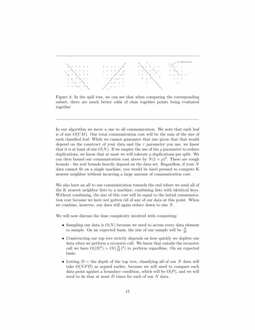
Figure 4: In the spill tree, we can see that when comparing the correspondingsubset, there are much better odds of close together points being evaluatedtogether

In our algorithm we incur a one to all communication. We note that each leafis of size O(UM). Our total communication cost will be the sum of the size ofeach classified leaf. While we cannot guarantee that size given that that woulddepend on the construct of your data and the τ parameter you use, we knowthat it is at least of size O(N). If we employ the use of the ρ parameter to reduceduplications, we know that at most we will tolerate ρ duplications per split. Wecan then bound our communication cost above by N(1 + ρ)d. These are roughbounds - the real bounds heavily depend on the data set. Regardless, if your Ndata cannot fit on a single machine, you would be hard pressed to compute Knearest neighbor without incurring a large amount of communication cost.

We also have an all to one communication towards the end where we send all ofthe K nearest neighbor lists to a machine, combining lists with identical keys.Without combining, the size of this cost will be equal to the initial communica-tion cost because we have not gotten rid of any of our data at this point. Whenwe combine, however, our data will again reduce down to size N .

We will now discuss the time complexity involved with computing:

• Sampling our data is O(N) because we need to access every data elementto sample. On an expected basis, the size of our sample will be N

M

• Constructing our top tree strictly depends on how quickly we deplete ourdata when we perform a recursive call. We know that outside the recursivecall we have O(|S|2) = O((NM )2) to perform regardless. On an expectedbasis.

• Letting D = the depth of the top tree, classifying all of our N data willtake O(NPD) as argued earlier, because we will need to compare eachdata point against a boundary condition, which will be O(P ), and we willneed to do that at most D times for each of our N data.

15

• Once we have our data on each machine, each of expected size UM , wewill need to compute another spill tree on each machine, again at leastO((UM)2).

• Assuming we use the same threshold U for our top and bottom tree, theleaves of each bottom tree will be size O(U). Again, the number of leavesdepends on our choice of τ , ρ, and U , as well as our data shape. However,each leaf will compute a naive K nearest neighbor, which is O(PU2).

We notice from the above complexity analysis that the total time complexityrequires us to know how many leaves we have in the top tree and the bottomtrees. Our hope is that the number of leaves is such that our total time com-plexity is such that it is less than our naive O(N2P ) method of computingK nearest neighbors. Regardless, if our data cannot fit on a single machine,we cannot hope to compute K nearest neighbor anyway without a distributedenvironment.

We notice that one of the advantages to our algorithm is that the runtime isheavily modifiable. Some of our user parameters such as M and U are tunedaccording to memory constraints or dataset size, but we can adjust τ and ρ tobring down the runtime of our algorithm at the expense of accuracy, or increasethe accuracy at the expense of the runtime [6]. Once you fit an initial modelit is convenient to be able to optimize your accuracy, subject to your personaltime constraints. Consider our top tree, we know that when τ is 0 the modelbecomes metric, and that as τ increases the overlap will become greater andgreater between pairs of children nodes. It is therefore important to keep τrelatively low in the top tree, where a large amount of overlap will result in agreater compute time in the top tree, as well as many more computations downthe line when we are using our bottom trees [6]. In the bottom trees, however,it is less important to keep τ low, as multiple machines are making their spilltree computations in parallel, and we can afford to allow more overlap, as longas we set an appropriate value for ρ to prevent the tree depth from getting outof hand. Overall, the user defined parameters give our model a large degree ofcustomization, and allow it to become optimized for the problem at hand.

5 Conclusion

We have seen two methods of distributing K nearest neighbors. The directapproach exhibits rather large communication costs as we need to duplicate ourdata multiple times (O(NM)) to implement it. It does, however, have reducedcomplexity; linear in the number of machines that we have.

16

Our second approach is to approximate our K nearest neighbors with hybridspill trees. The exact time complexity and communication cost is highly de-pendent on your data as well as some of your model parameters (namely yourresampling parameters). Further emperical analysis will need to be completedto flesh out how dependent these features are on runtime and communicationcost. It should be noted, however, that despite these uncertainties you may stillhave to implement your problem in this manner because of your data size. Ifyour data is too big to fit on one machine, there is little you can do to avoidhigh communication costs when trying to implement K nearest neighbors on adistributed framework.

6 References

[1]: Richard Duda, Peter Hart, David Stork Duda. “Pattern Classification”p.18-30, 2001.

[2]: Saravanan Thirumuruganathan. “A Detailed Introduction to K-NearestNeighbor (KNN) Algorithm”, 2010.

[3]: Ali Dashti. “Efficient Computation Of K-Nearest Neighbor Graphs ForLarge High-Dimensional Data Sets On GPU Clusters”, 2013.

[4]: Wei Dong, Moses Charikar, Kai Li. “Efcient K-Nearest Neighbor GraphConstruction for Generic Similarity Measures”, 2011.

[5]: Ting Liu, Andrew W. Moore, Alexander Gray, Ke Yang. “An Investigationof Practical Approximate Nearest Neighbor Algorithms”, 2004.

[6]: Ting Liu, Charles Rosenberg, Henry Rowley. “Clustering Billions of Imageswith Large Scale Nearest Neighbor Search”, 2007.

17