1

Distributed Localization and Tracking of Mobile

Networks Including Noncooperative Objects

Florian Meyer, Member, IEEE, Ondrej Hlinka, Henk Wymeersch, Member, IEEE, Erwin Riegler, Member, IEEE,

and Franz Hlawatsch, Fellow, IEEE

Abstract—We propose a Bayesian method for distributed se-

quential localization of mobile networks composed of both coop-

erative agents and noncooperative objects. Our method provides

a consistent combination of cooperative self-localization (CS) and

distributed tracking (DT). Multiple mobile agents and objects

are localized and tracked using measurements between agents

and objects and between agents. For a distributed operation and

low complexity, we combine particle-based belief propagation

with a consensus or gossip scheme. High localization accuracy

is achieved through a probabilistic information transfer between

the CS and DT parts of the underlying factor graph. Simulation

results demonstrate significant improvements in both agent self-

localization and object localization performance compared to

separate CS and DT, and very good scaling properties with

respect to the numbers of agents and objects.

Index Terms—Agent network, belief propagation, consensus,

cooperative localization, distributed estimation, distributed track-

ing, factor graph, gossip, message passing, sensor network.

I. INTRODUCTION

A. Background and State of the Art

Cooperative self-localization (CS) [1], [2] and distributed

tracking (DT) [3] are key signal processing tasks in de-

centralized agent networks. Applications include surveillance

[4], environmental and agricultural monitoring [5], robotics

[6], and pollution source localization [7]. In CS, each agent

measures quantities related to the location of neighboring

agents relative to its own location. By cooperating with other

agents, it is able to estimate its own location. In DT, the

measurements performed by the agents are related to the

locations (or, more generally, states) of noncooperative objects

to be tracked. At each agent, estimates of the object states

are cooperatively calculated from all agent measurements. CS

and DT are related since, ideally, an agent needs to know

its own location to be able to contribute to DT. This relation

Final manuscript, February 25, 2016. To appear in the IEEE Transactionson Signal and Information Processing over Networks.

F. Meyer and F. Hlawatsch are with the Institute of Telecommunications,TU Wien, 1040 Vienna, Austria (email: {fmeyer, fhlawats}@nt.tuwien.ac.at).O. Hlinka is with robart GmbH, 4020 Linz, Austria (e-mail: on-drej.hlinka@robart.cc). H. Wymeersch is with the Department of Signals andSystems, Chalmers University of Technology, Gothenburg 41296, Sweden(email: henk.wymeersch@ieee.org). E. Riegler is with the Department of In-formation Technology and Electrical Engineering, ETH Zurich, 8092 Zurich,Switzerland (email: eriegler@nari.ee.ethz.ch). This work was supported by theFWF under Grants S10603-N13 and P27370-N30, by the WWTF under GrantICT10-066 (NOWIRE), and by the European Commission under ERC GrantNo. 258418 (COOPNET), the Newcom# Network of Excellence in WirelessCommunications, and the National Sustainability Program (Grant LO1401).This work was partly presented at the 46th Asilomar Conference on Signals,Systems and Computers, Pacific Grove, CA, Nov. 2012.

motivates the combined CS-DT method proposed in this paper,

which achieves improved performance through a probabilistic

information transfer between CS and DT.

For CS of static agents (hereafter termed “static CS”), the

nonparametric belief propagation (BP) algorithm has been

proposed in [8]. BP schemes are well suited to CS because

their complexity scales only linearly with the number of agents

and, under mild assumptions, a distributed implementation

is easily obtained. In [2], a distributed BP message passing

algorithm for CS of mobile agents (hereafter termed “dynamic

CS”) is proposed. A message passing algorithm based on the

mean field approximation is presented for static CS in [9].

In [10] and [11], nonparametric BP is extended to dynamic

CS and combined with a parametric message representation.

In [12], a particle-based BP method using a Gaussian belief

approximation is proposed. The low-complexity method for

dynamic CS presented in [13] is based on the Bayesian

filter and a linearized measurement equation. Another low-

complexity CS method with low communication requirements

is sigma point BP [14]. In [15], a censoring scheme for sigma

point BP is proposed to further reduce communications.

For DT, various distributed recursive estimation methods are

available, e.g., [16]–[20]. Distributed particle filters [18] are

especially attractive since they are suited to nonlinear, non-

Gaussian systems. In particular, in the distributed particle fil-

ters proposed in [19] and [20], consensus algorithms are used

to compute global particle weights reflecting the measurements

of all agents. For DT of an unknown, possibly time-varying

number of objects in the presence of object-to-measurement

association uncertainty, methods based on random finite sets

are proposed in [21]–[23].

In the framework of simultaneous localization and tracking

(SLAT), static agents track a noncooperative object and local-

ize themselves, using measurements of the distances between

each agent and the object [24]. In contrast to dynamic CS,

measurements between agents are only used for initialization.

A centralized particle-based SLAT method using BP is pro-

posed in [25]. Distributed SLAT methods include a technique

using a Bayesian filter and communication via a junction tree

[26], iterative maximum likelihood methods [27], variational

filtering [28], and particle-based BP [29].

B. Contributions and Paper Organization

We propose a method for distributed localization and track-

ing of cooperative agents and noncooperative objects in wire-

less networks, using measurements between agents and objects

and between agents. This method, for the first time, provides

2

a consistent combination of CS and DT in decentralized agent

networks where the agents and objects may be mobile. To the

best of our knowledge, it is the first method for simultaneous

CS and DT in a dynamic setting. It is different from SLAT

methods in that the agents may be mobile and measurements

between the agents are used also during runtime. A key feature

of our method is a probabilistic information transfer between

the CS and DT stages, which allows uncertainties in one stage

to be taken into account by the other stage and thereby can

improve the performance of both stages.

Contrary to the multitarget tracking literature [30], [31], we

assume that the number of objects is known and the objects

can be identified by the agents. Even with this assumption, the

fact that the agents may be mobile and their states are unknown

causes the object localization problem to be more challenging

than in the setting of static agents with known states. This

is because the posterior distributions of the object and agent

states are coupled through recurrent pairwise measurements,

and thus all these states should be estimated jointly and

sequentially. This joint, sequential estimation is performed

quite naturally through our factor graph formulation of the

entire estimation problem and the use of BP message passing.

In addition, BP message passing facilitates a distributed im-

plementation and exhibits very good scalability in the numbers

of agents and objects. We also present a new particle-based

implementation of BP message passing that is less complex

than conventional nonparametric BP [8], [10].

Our method is an extension of BP-based dynamic CS [2],

[10], [11] to include noncooperative objects. This extension

is nontrivial because, contrary to pure CS, the communication

and measurement topologies (graphs) do not match. Indeed,

because the objects do not communicate, certain messages

needed to calculate the object beliefs are not available at the

agents. The proposed method employs a consensus scheme

[19] for a distributed calculation of these messages. The re-

sulting combination of BP and consensus may also be useful in

other distributed inference problems involving noncooperative

objects.

This paper is organized as follows. The system model is

described in Section II. A BP message passing scheme for joint

CS and DT is developed in Section III, and a particle-based

implementation of this scheme in Section IV. A distributed

localization-and-tracking algorithm that combines particle-

based BP and consensus is presented in Section V. The algo-

rithm’s communication requirements and delay are analyzed in

Section VI. Finally, simulation results are presented in Section

VII. This paper extends our previous work in [32] and [33] in

the following respects: we consider multiple objects, introduce

a new low-complexity message multiplication scheme, provide

an analysis of communication requirements and delay, present

a numerical comparison with particle filtering and a numerical

analysis of scaling properties, and demonstrate performance

gains over separate CS and DT in a static scenario (in addition

to two dynamic scenarios). We note that an extension of the

proposed method including a distributed information-seeking

controller optimizing the behavior (e.g., movement) of the

agents is presented in [34].

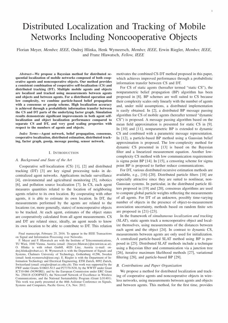
cooperative agent

noncooperative object

communication link

measurement

MOl,n

MAl,n Ml,nagent l

agent l′

objectm

Cl′,n

Am,n

Fig. 1. Network with cooperative agents and noncooperative objects. Alsoshown are the sets Ml,n, MA

l,n, and MO

l,nfor a specific agent l, the set

Cl′,n for a specific agent l′, and the set Am,n for a specific object m.

II. SYSTEM MODEL AND PROBLEM STATEMENT

A. System Model

We consider a decentralized network of cooperative agents

and noncooperative objects as shown in Fig. 1. We denote

by A ⊆ N the set of agents, by O ⊆ N the set of objects,

and by E , A ∪ O the set of all entities (agents and

objects). We use the indices k ∈ E , l ∈ A, and m ∈ O to

denote a generic entity, an agent, and an object, respectively.

The numbers of agents and objects are assumed known. The

objects are noncooperative in that they do not communicate,

do not perform computations, and do not actively perform any

measurements. The state of entity k ∈E at time n∈ {0, 1, . . .},

denoted xk,n, consists of the current location and, possibly,

motion parameters such as velocity [35]. The states evolve

according to

xk,n = g(xk,n−1,uk,n) , k ∈E , (1)

where uk,n denotes driving noise with probability density

function (pdf) f(uk,n). The statistical relation between xk,n−1

and xk,n defined by (1) can also be described by the state-

transition pdf f(xk,n|xk,n−1).The communication and measurement topologies are de-

scribed by sets Cl,n and Ml,n as follows. Agent l ∈ A is

able to communicate with agent l′ if l′ ∈ Cl,n ⊆ A \ {l}.

Communication is symmetric, i.e., l′ ∈ Cl,n implies l ∈ Cl′,n.

Furthermore, agent l ∈ A acquires a measurement yl,k;n

relative to agent or object k ∈ E if k∈Ml,n ⊆ E \{l}. Note

that Cl,n consists of all agents that can communicate with agent

l ∈ A, and Ml,n consists of all entities measured by agent

l ∈ A. Thus, there are actually two networks: one is defined by

the communication graph, i.e., by Cl,n for l ∈ A, and involves

only agents; the other is defined by the measurement graph,

i.e., by Ml,n for l ∈ A, and involves agents and objects. The

communication graph is assumed to be connected. We also

define MAl,n,Ml,n∩A and MO

l,n,Ml,n∩O, i.e., the subsets

of Ml,n containing only agents and only objects, respectively,

and Am,n , {l ∈ A|m ∈ MOl,n}, i.e., the set of agents that

acquire measurements of object m. Note that m ∈ MOl,n if

and only if l ∈ Am,n. We assume that MAl,n ⊆ Cl,n, i.e., if

agent l acquires a measurement relative to agent l′, it is able

to communicate with agent l′. The sets Cl,n etc. may be time-

dependent. An example of communication and measurement

topologies is given in Fig. 1.

3

We consider “pairwise” measurements yl,k;n that depend on

the states xl,n and xk,n according to

yl,k;n = h(xl,n,xk,n,vl,k;n) , l ∈A , k ∈Ml,n . (2)

Here, vl,k;n is measurement noise with pdf f(vl,k;n). An

example is the scalar “noisy distance” measurement

yl,k;n = ‖xl,n− xk,n‖+ vl,k;n , (3)

where xk,n represents the location of entity k (this is part

of the state xk,n). The statistical dependence of yl,k;n on

xl,n and xk,n is described by the local likelihood function

f(yl,k;n|xl,n,xk,n). We denote by xn ,(

xk,n

)

k∈Eand yn ,

(

yl,k;n

)

l∈A, k∈Ml,nthe vectors of, respectively, all states and

measurements at time n. Furthermore, we define x1:n ,(

xT1 · · · x

Tn

)Tand y1:n ,

(

yT1 · · · y

Tn

)T.

B. Assumptions

We will make the following commonly used assumptions,

which are reasonable in many practical scenarios [2].

(A1) All agent and object states are independent a priori at

time n=0, i.e., f(x0) =∏

k∈E f(xk,0).(A2) All agents and objects move according to a memory-

less walk, i.e., f(x1:n) = f(x0)∏n

n′=1 f(xn′ |xn′−1).(A3) The state transitions of the various agents and objects

are independent, i.e., f(xn|xn−1) =∏

k∈E f(xk,n|xk,n−1).(A4) The current measurements yn are conditionally inde-

pendent, given the current states xn, of all the other states and

of all past and future measurements, i.e., f(yn|x0:∞,y1:n−1,yn+1:∞) = f(yn|xn).

(A5) The current states xn are conditionally independent of

all past measurements, y1:n−1, given the previous states xn−1,

i.e., f(xn|xn−1,y1:n−1) = f(xn|xn−1).(A6) The measurements yl,k;n and yl′,k′;n are condition-

ally independent given xn unless (l, k) = (l′, k′), and each

measurement yl,k;n depends only on the states xl,n and

xk,n. Together with (A4), this leads to the following fac-

torization of the “total” likelihood function: f(y1:n|x1:n) =∏n

n′=1

∏

l∈A

∏

k∈Ml,nf(yl,k;n′ |xl,n′ ,xk,n′).

We also assume that the objects can be identified by the

agents, i.e., object-to-measurement associations are known.

(We note that BP-based methods for multitarget tracking in

the presence of object-to-measurement association uncertainty

were recently proposed in [36] and [37]; however, these

methods are not distributed.) Furthermore, we assume that

each agent l ∈A knows the functional forms of its own state-

transition pdf and initial state pdf as well as of those of all

objects, i.e., f(xk,n|xk,n−1) and f(xk,0) for k ∈ {l} ∪ O.

Finally, all prior location and motion information is available

in one global reference frame, and the internal clocks of all

agents are synchronous (see [38]–[40] for distributed clock

synchronization algorithms).

C. Problem Statement

The task we consider is as follows: Each agent l ∈ Aestimates its own state xl,n and all object states xm,n,

m ∈ O from the entire measurement vector y1:n =(

yl′,k;n′

)

l′∈A, k∈Ml′,n′ ,n′∈{1,...,n}, i.e., from the pairwise mea-

surements between the agents and between the agents and

objects up to time n. This is to be achieved using only

communication with the “neighbor agents” as defined by Cl,n,

and without transmitting measurements between agents.

In this formulation of the estimation task, compared to pure

CS of cooperative agents (e.g., [2]) or pure DT of noncoop-

erative objects (e.g., [20]), the measurement set is extended

in that it includes also the respective other measurements—

i.e., the measurements between agents and objects for agent

state estimation and those between agents for object state

estimation. This explains why the proposed algorithm is able

to outperform separate CS and DT. In fact, by using all the

present and past measurements available throughout the entire

network, the inherent coupling between the CS and DT tasks

can be exploited for improved performance.

III. BP MESSAGE PASSING SCHEME

In this section, we describe a BP message passing scheme

for the joint CS-DT problem. A particle-based implementation

of this scheme will be presented in Section IV, and the final

distributed algorithm will be developed in Section V.

For estimating the agent or object state xk,n, k ∈ E from

y1:n, a popular Bayesian estimator is the minimum mean-

square error (MMSE) estimator given by [41]

xMMSEk,n ,

∫

xk,nf(xk,n|y1:n)dxk,n . (4)

This estimator involves the “marginal” posterior pdf

f(xk,n|y1:n), k ∈ E , which can be obtained by marginal-

izing the “joint” posterior pdf f(x1:n|y1:n). However, direct

marginalization of f(x1:n|y1:n) is infeasible because it relies

on nonlocal information and involves integration in spaces

whose dimension grows with time and network size. This

problem can be addressed by using a particle-based, distributed

BP scheme that takes advantage of the temporal and spatial

independence structure of f(x1:n|y1:n) and avoids explicit

integration. The independence structure corresponds to the

following factorization of f(x1:n|y1:n), which is obtained by

using Bayes’ rule and assumptions (A1)–(A6):

f(x1:n|y1:n) ∝

(

∏

k∈E

f(xk,0)

)

×n∏

n′=1

(

∏

k1∈E

f(xk1,n′ |xk1,n′−1)

)

×∏

l∈A

∏

k2∈Ml,n′

f(yl,k2;n′ |xl,n′ ,xk2,n′) . (5)

Here, ∝ denotes equality up to a constant normalization factor.

A. The Message Passing Scheme

The proposed BP message passing scheme uses the sum-

product algorithm [42] to produce approximate marginal

posterior pdfs (“beliefs”) b(xk,n) ≈ f(xk,n|y1:n), k ∈ E .

This is based on the factor graph [43] corresponding to the

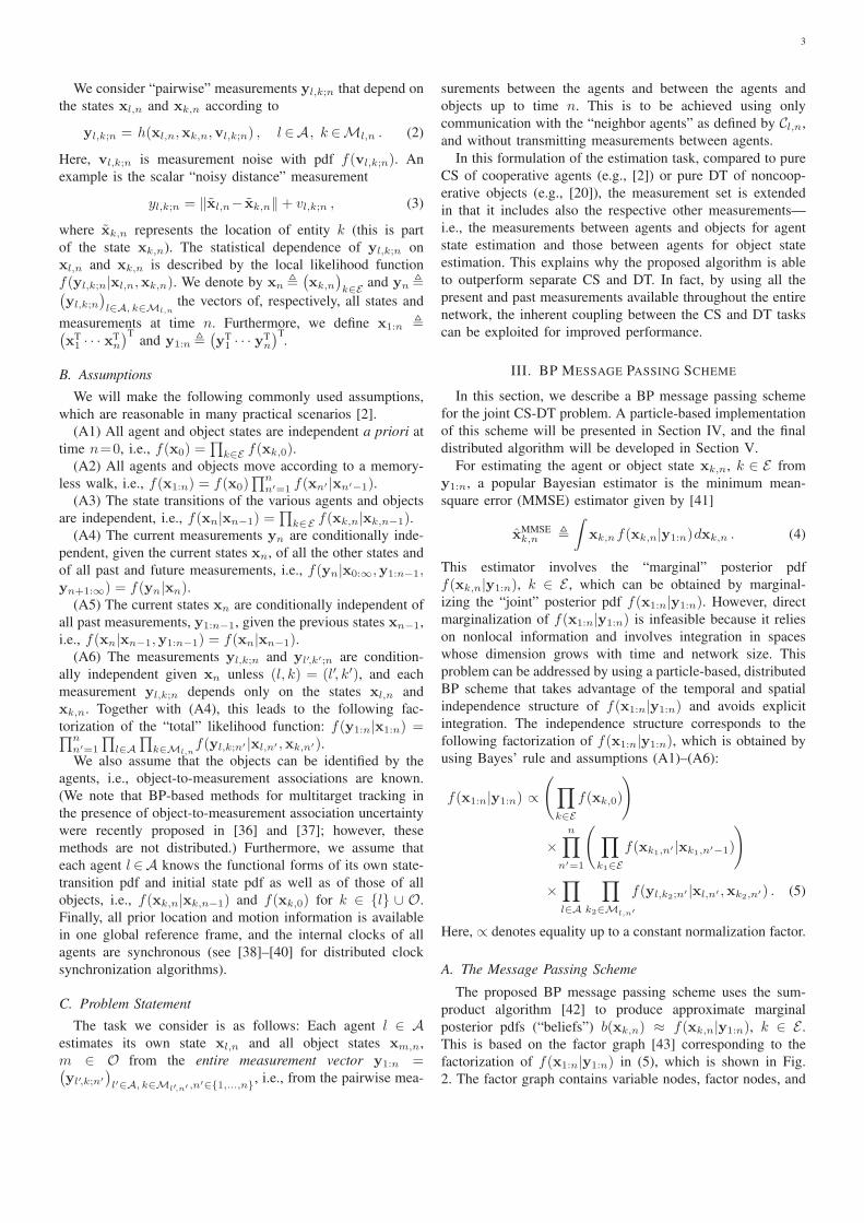
factorization of f(x1:n|y1:n) in (5), which is shown in Fig.

2. The factor graph contains variable nodes, factor nodes, and

4

x1

x2

x1

x2

f1f1

f2f2

n−1 n

f1,2

f2,1f2,1

f1,l f1,lf1,2

f2,lf2,l

b(P )1

b(p−1)2b

(p−1)l

φ(p)l→1

φ(p)2→1

φ→n

xm xm

fm fm

f2,m

f1,m

φ(p)1→m

ψ(p−1)1→m

φ(p)l→m

ψ(p−1)m→1

φ(p)m→1

φ→nb(P )m

Fig. 2. Factor graph showing the states of agents l = 1 and l = 2 and of

a single object m at time instants n− 1 and n, assuming 2 ∈ C1,n and

m ∈ MO1,n ∩ MO

2,n−1. Variable and factor nodes are depicted as circles

and squares, respectively. Time indices are omitted for simplicity. The short

notation fk , f(xk,n′ |xk,n′−1), fl,k , f(yl,k;n′ |xl,n′ ,xk,n′ ), b(p)k

,

b(p)(xk,n′ ), ψ(p)k→k′ , ψ

(p)k→k′ (xk,n′ ), etc. (for n′ ∈ {1, . . . , n}) is used.

The upper two (black) dotted boxes correspond to the CS part (for agents l=

1, 2); the bottom (red) dotted box corresponds to the DT part. Edges between

black dotted boxes imply communication between agents. Only messages and

beliefs involved in the computation of b(p)(x1,n) and b(p)(xm,n) are shown.

Edges with non-filled arrowheads depict particle-based messages and beliefs,

while edges with filled arrowheads depict messages involved in the consensus

scheme.

edges connecting certain variable nodes with certain factor

nodes. Because the factor graph is loopy (i.e., some edges form

loops), BP schemes provide only an approximate marginaliza-

tion. However, the resulting beliefs have been observed to be

quite accurate in many applications [2], [42], [44]. In loopy

factor graphs, the BP scheme becomes iterative, and there exist

different orders in which messages can be computed [2], [42],

[44].

Here, we choose an order that enables real-time processing

and facilitates a distributed implementation. More specifically,

the belief of agent node l ∈A and object node m∈O at time

n and message passing iteration p∈ {1, . . . , P} is given by

b(p)(xl,n) ∝ φ→n(xl,n)∏

k∈Ml,n

φ(p)k→l(xl,n) , l∈A (6)

b(p)(xm,n) ∝ φ→n(xm,n)∏

l∈Am,n

φ(p)l→m(xm,n) , m∈O , (7)

respectively, with the “prediction message”

φ→n(xk,n) =

∫

f(xk,n|xk,n−1)b(P )(xk,n−1)dxk,n−1 , k∈E

(8)

and the “measurement messages”

φ(p)k→l(xl,n) =

∫

f(yl,k;n|xl,n ,xk,n) b(p−1)(xk,n) dxk,n ,

k∈MAl,n , l∈A

∫

f(yl,k;n|xl,n ,xk,n)ψ(p−1)k→l (xk,n) dxk,n ,

k∈MOl,n , l∈A

(9)and

φ(p)l→m(xm,n) =

∫

f(yl,m;n|xl,n ,xm,n)ψ(p−1)l→m (xl,n) dxl,n ,

l∈Am,n , m∈O . (10)

Here, ψ(p−1)m→l (xm,n) and ψ

(p−1)l→m (xl,n) (constituting the “ex-

trinsic information”) are given by

ψ(p−1)m→l (xm,n) = φ→n(xm,n)

∏

l′∈Am,n\{l}

φ(p−1)l′→m(xm,n) (11)

ψ(p−1)l→m (xl,n) = φ→n(xl,n)

∏

k∈Ml,n\{m}

φ(p−1)k→l (xl,n) . (12)

This recursion is initialized with b(0)(xl,n) = φ→n(xl,n),

ψ(0)m→l(xm,n) = φ→n(xm,n), and ψ

(0)l→m(xl,n) = φ→n(xl,n).

The messages and beliefs involved in calculating b(p)(xl,n)and b(p)(xm,n) are shown in Fig. 2. We note that messages

entering or leaving an object variable node in Fig. 2 do not

imply that there occurs any communication involving objects.

B. Discussion

According to (6) and (7), the agent beliefs b(p)(xl,n)and object beliefs b(p)(xm,n) involve the product of all the

messages passed to the corresponding variable node l and

m, respectively. Similarly, according to (11) and (12), the

extrinsic informations ψ(p−1)m→l (xm,n) and ψ

(p−1)l→m (xl,n) involve

the product of all the messages passed to the corresponding

variable node m and l, respectively, except the message of

the receiving factor node f(yl,m;n|xl,n ,xm,n). Furthermore,

according to (9), the extrinsic information ψ(p−1)k→l (xk,n) passed

from variable node xk,n to factor node f(yk,l;n|xk,n ,xl,n) is

used for calculating the message φ(p)k→l(xl,n) passed from that

factor node to the respective other adjacent variable node xl,n.

A similar discussion applies to (10) and ψ(p−1)l→m (xl,n).

Two remarks are in order. First, for low complexity, com-

munication requirements, and latency, messages are sent only

forward in time and iterative message passing is performed

for each time individually. As a consequence, the message

(extrinsic information) from variable node xk,n−1 to factor

node f(xk,n|xk,n−1) equals the belief b(P )(xk,n−1) (see (8)),

and φ→n(xk,n) in (8) (for n fixed) remains unchanged during

all message passing iterations. Second, for any k ∈ A, as no

information from the factor node f(yl,k;n|xl,n,xk,n) is used

in the calculation of b(p−1)(xk,n) according to (6) and (9),

b(p−1)(xk,n) is used in (9) as the extrinsic information passed

to the factor node f(yl,k;n|xl,n,xk,n). A similar message

computation order is used in the SPAWN algorithm for CS

[2], [10]. This order significantly reduces the computational

complexity since it avoids the computation of extrinsic in-

formations exchanged among agent variable nodes. It also

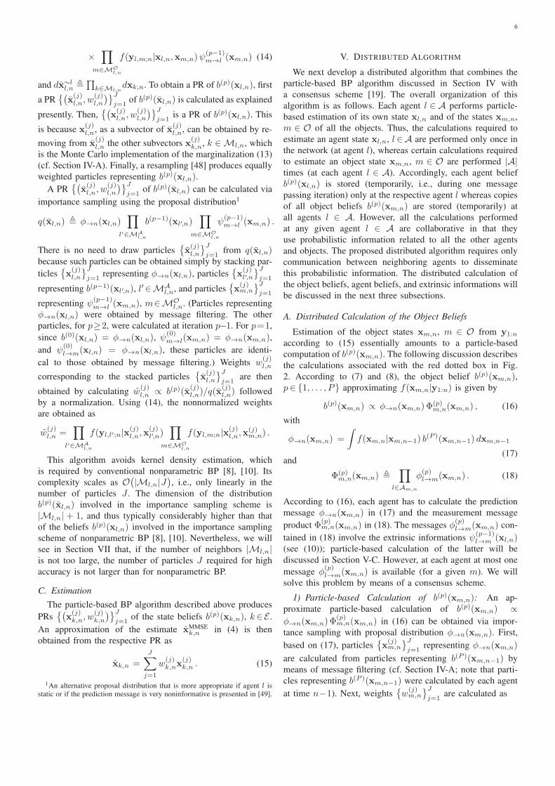
5

CS

DT

CS

DT

b(P )A,n−1 b

(P )A,n−1

b(P )O,n−1 b

(P )O,n−1

b(P )A,n

b(P )O,n

b(P )A,n

b(P )O,n

x(P )A,n

ψ(p)A→O,n ψ

(p)O→A,n

(a) (b)

Fig. 3. Block diagram of (a) separate CS and DT and (b) the proposed scheme,

with b(P )A,n

,{

b(P )(xl,n)}

l∈A, b

(P )O,n

,{

b(P )(xm,n)}

m∈O, ψ

(p)A→O,n

,{

ψ(p)l→m

(xl,n)}

l∈Am,n,m∈O, ψ

(p)O→A,n

,{

ψ(p)m→l

(xm,n)}

m∈MOl,n

, l∈A,

and x(P )A,n

,(

x(P )l,n

)

l∈A. In separate CS and DT, the final agent state estimates

x(P )A,n

are transferred from CS to DT. In the proposed scheme, probabilistic

information (the extrinsic informations ψ(p)A→O,n

and ψ(p)O→A,n

) is transferred

between CS and DT in each message passing iteration p.

reduces the amount of communication between agents because

beliefs passed between agents can be broadcast, whereas

the exchange of extrinsic information would require separate

point-to-point communications between agents [2], [10].

Contrary to classical sequential Bayesian filtering [45],

which only exploits the temporal conditional independence

structure of the estimation problem, the proposed BP scheme

(6)–(12) also exploits the spatial conditional independency

structure. In fact, increasing the number of agents or objects

leads to additional variable nodes in the factor graph but not

to a higher dimension of the messages passed between the

nodes. As a consequence, the computational complexity scales

very well in the numbers of agents and objects. As verified

in Section VII-C, a comparable scaling behavior cannot be

achieved with classical Bayesian filtering techniques.

The factor graph in Fig. 2 and the corresponding BP

scheme (6)–(12) combine CS and DT into a unified, coherent

estimation technique. Indeed, in contrast to the conventional

approach of separate CS and DT—i.e., first performing CS to

localize the agents and then, based on the estimated agent

locations, performing DT to localize the objects—our BP

scheme exchanges probabilistic information between the CS

and DT parts of the factor graph. Thereby, uncertainties in

one stage are taken into account by the respective other

stage, and the performance of both stages can be improved.

This information transfer, which will be further discussed in

Sections V-A and V-B, is the main reason for the superior

performance of the proposed joint CS-DT algorithm; it is

visualized and contrasted with the conventional approach in

Fig. 3.

IV. PARTICLE-BASED PROCESSING

Because of the nonlinear and non-Gaussian state transition

model (1) and measurement model (2), a closed-form eval-

uation of the integrals and message products in (6)–(12) is

typically impossible. Therefore, we next present a new low-

complexity particle-based implementation of the BP scheme

(6)–(12). This implementation uses particle representations

(PRs) of beliefs and messages, which approximate distribu-

tions in terms of randomly drawn particles (samples) x(j)

and weights w(j), for j ∈ {1, . . . , J}. As in conventional

nonparametric BP [8], [10], the operations of message filtering

and message multiplication are performed. Message filtering

calculates the prediction message (8) and equals the message

filtering operation of nonparametric BP. However, for mes-

sage multiplication in (6), (7), (11), and (12), the “stacking

technique” introduced in [14] is used. This technique avoids

an explicit calculation of the measurement messages (9) and

(10) and does not use computationally intensive kernel density

estimates, which are required by nonparametric BP. Thereby,

its complexity is only linear in the number of particles. We

note that an alternative message multiplication scheme that

also avoids the use of kernel density estimates and whose

complexity is linear in the number of particles was proposed

in [46]. This scheme constructs an approximate proposal

distribution in order to calculate weighted particles for beliefs

and messages. Our approach is different in that the proposal

distribution is formed simply by “stacking” incoming beliefs,

and the calculation of particles and weights for incoming

messages is avoided (see Section IV-B).

A. Message Filtering

The message filtering operation reviewed in the following

is analogous to the prediction step of the sampling impor-

tance resampling particle filter [47]. Particle-based calcula-

tion of (8) means that we obtain a PR{(

x(j)k,n, w

(j)k,n

)}J

j=1

of φ→n(xk,n) =∫

f(xk,n|xk,n−1) b(P )(xk,n−1)dxk,n−1

from a PR{(

x(j)k,n−1, w

(j)k,n−1

)}J

j=1of b(P )(xk,n−1). This

can be easily done by recognizing that the above inte-

gral is a marginalization of f(xk,n|xk,n−1) b(P )(xk,n−1).

Motivated by this interpretation, we first establish a PR{(

x(j)k,n,x

(j)k,n−1, w

(j)k,n−1

)}J

j=1of f(xk,n|xk,n−1)b

(P )(xk,n−1)

by drawing for each particle(

x(j)k,n−1, w

(j)k,n−1

)

representing

b(P )(xk,n−1) one particle x(j)k,n from f(xk,n|x

(j)k,n−1). Then,

removing{

x(j)k,n−1

}J

j=1from

{(

x(j)k,n,x

(j)k,n−1, w

(j)k,n−1

)}J

j=1is

the Monte Carlo implementation of the above marginalization

[48]. This means that{(

x(j)k,n, w

(j)k,n

)}J

j=1with w

(j)k,n = w

(j)k,n−1

for all j ∈ {1, . . . , J} constitutes the desired PR of φ→n(xk,n).

B. Message Multiplication

Next, we propose a message multiplication scheme for cal-

culating the beliefs in (6) and (7) and the extrinsic informations

in (11) and (12). For concreteness, we present the calculation

of the agent beliefs (6); the object beliefs (7) and extrinsic

informations (11) and (12) are calculated in a similar manner.

Following [14], we consider the “stacked state” xl,n ,(

xk,n

)

k∈{l}∪Ml,n, which consists of the agent state xl,n and

the states xk,n of all measurement partners k ∈ Ml,n of agent

l. Using (9) in (6), one readily obtains

b(p)(xl,n) =

∫

b(p)(xl,n) dx∼ll,n , (13)

where

b(p)(xl,n) ∝ φ→n(xl,n)

×∏

l′∈MAl,n

f(yl,l′;n|xl,n,xl′,n) b(p−1)(xl′,n)

6

×∏

m∈MOl,n

f(yl,m;n|xl,n,xm,n)ψ(p−1)m→l (xm,n) (14)

and dx∼ll,n ,

∏

k∈Ml,ndxk,n. To obtain a PR of b(p)(xl,n), first

a PR{(

x(j)l,n, w

(j)l,n

)}J

j=1of b(p)(xl,n) is calculated as explained

presently. Then,{(

x(j)l,n, w

(j)l,n

)}J

j=1is a PR of b(p)(xl,n). This

is because x(j)l,n, as a subvector of x

(j)l,n, can be obtained by re-

moving from x(j)l,n the other subvectors x

(j)k,n, k ∈ Ml,n, which

is the Monte Carlo implementation of the marginalization (13)

(cf. Section IV-A). Finally, a resampling [48] produces equally

weighted particles representing b(p)(xl,n).

A PR{(

x(j)l,n, w

(j)l,n

)}J

j=1of b(p)(xl,n) can be calculated via

importance sampling using the proposal distribution1

q(xl,n) , φ→n(xl,n)∏

l′∈MAl,n

b(p−1)(xl′,n)∏

m∈MOl,n

ψ(p−1)m→l (xm,n) .

There is no need to draw particles{

x(j)l,n

}J

j=1from q(xl,n)

because such particles can be obtained simply by stacking par-

ticles{

x(j)l,n

}J

j=1representing φ→n(xl,n), particles

{

x(j)l′,n

}J

j=1

representing b(p−1)(xl′,n), l′∈MA

l,n, and particles{

x(j)m,n

}J

j=1

representing ψ(p−1)m→l (xm,n), m∈MO

l,n. (Particles representing

φ→n(xl,n) were obtained by message filtering. The other

particles, for p≥2, were calculated at iteration p−1. For p=1,

since b(0)(xl,n) = φ→n(xl,n), ψ(0)m→l(xm,n) = φ→n(xm,n),

and ψ(0)l→m(xl,n) = φ→n(xl,n), these particles are identi-

cal to those obtained by message filtering.) Weights w(j)l,n

corresponding to the stacked particles{

x(j)l,n

}J

j=1are then

obtained by calculating w(j)l,n ∝ b(p)(x

(j)l,n)/q(x

(j)l,n) followed

by a normalization. Using (14), the nonnormalized weights

are obtained as

w(j)l,n =

∏

l′∈MAl,n

f(yl,l′;n|x(j)l,n,x

(j)l′,n)

∏

m∈MOl,n

f(yl,m;n|x(j)l,n,x

(j)m,n) .

This algorithm avoids kernel density estimation, which

is required by conventional nonparametric BP [8], [10]. Its

complexity scales as O(

|Ml,n|J)

, i.e., only linearly in the

number of particles J . The dimension of the distribution

b(p)(xl,n) involved in the importance sampling scheme is

|Ml,n| + 1, and thus typically considerably higher than that

of the beliefs b(p)(xl,n) involved in the importance sampling

scheme of nonparametric BP [8], [10]. Nevertheless, we will

see in Section VII that, if the number of neighbors |Ml,n|is not too large, the number of particles J required for high

accuracy is not larger than for nonparametric BP.

C. Estimation

The particle-based BP algorithm described above produces

PRs{(

x(j)k,n, w

(j)k,n

)}J

j=1of the state beliefs b(p)(xk,n), k∈E .

An approximation of the estimate xMMSEk,n in (4) is then

obtained from the respective PR as

xk,n =

J∑

j=1

w(j)k,nx

(j)k,n . (15)

1An alternative proposal distribution that is more appropriate if agent l isstatic or if the prediction message is very noninformative is presented in [49].

V. DISTRIBUTED ALGORITHM

We next develop a distributed algorithm that combines the

particle-based BP algorithm discussed in Section IV with

a consensus scheme [19]. The overall organization of this

algorithm is as follows. Each agent l ∈ A performs particle-

based estimation of its own state xl,n and of the states xm,n,

m ∈ O of all the objects. Thus, the calculations required to

estimate an agent state xl,n, l ∈A are performed only once in

the network (at agent l), whereas certain calculations required

to estimate an object state xm,n, m ∈ O are performed |A|times (at each agent l ∈ A). Accordingly, each agent belief

b(p)(xl,n) is stored (temporarily, i.e., during one message

passing iteration) only at the respective agent l whereas copies

of all object beliefs b(p)(xm,n) are stored (temporarily) at

all agents l ∈ A. However, all the calculations performed

at any given agent l ∈ A are collaborative in that they

use probabilistic information related to all the other agents

and objects. The proposed distributed algorithm requires only

communication between neighboring agents to disseminate

this probabilistic information. The distributed calculation of

the object beliefs, agent beliefs, and extrinsic informations will

be discussed in the next three subsections.

A. Distributed Calculation of the Object Beliefs

Estimation of the object states xm,n, m ∈ O from y1:n

according to (15) essentially amounts to a particle-based

computation of b(p)(xm,n). The following discussion describes

the calculations associated with the red dotted box in Fig.

2. According to (7) and (8), the object belief b(p)(xm,n),p∈ {1, . . . , P} approximating f(xm,n|y1:n) is given by

b(p)(xm,n) ∝ φ→n(xm,n) Φ(p)m,n(xm,n) , (16)

with

φ→n(xm,n) =

∫

f(xm,n|xm,n−1) b(P )(xm,n−1) dxm,n−1

(17)and

Φ(p)m,n(xm,n) ,

∏

l∈Am,n

φ(p)l→m(xm,n) . (18)

According to (16), each agent has to calculate the prediction

message φ→n(xm,n) in (17) and the measurement message

product Φ(p)m,n(xm,n) in (18). The messages φ

(p)l→m(xm,n) con-

tained in (18) involve the extrinsic informations ψ(p−1)l→m (xl,n)

(see (10)); particle-based calculation of the latter will be

discussed in Section V-C. However, at each agent at most one

message φ(p)l→m(xm,n) is available (for a given m). We will

solve this problem by means of a consensus scheme.

1) Particle-based Calculation of b(p)(xm,n): An ap-

proximate particle-based calculation of b(p)(xm,n) ∝

φ→n(xm,n) Φ(p)m,n(xm,n) in (16) can be obtained via impor-

tance sampling with proposal distribution φ→n(xm,n). First,

based on (17), particles{

x(j)m,n

}J

j=1representing φ→n(xm,n)

are calculated from particles representing b(P )(xm,n−1) by

means of message filtering (cf. Section IV-A; note that parti-

cles representing b(P )(xm,n−1) were calculated by each agent

at time n−1). Next, weights{

w(j)m,n

}J

j=1are calculated as

7

w(j)m,n = Φ(p)

m,n(x(j)m,n) (19)

followed by a normalization. Finally, resampling is performed

to obtain equally weighted particles representing b(p)(xm,n).However, this particle-based implementation presupposes that

the message product Φ(p)m,n(xm,n) evaluated at the particles

{

x(j)m,n

}J

j=1is available at the agents.

2) Distributed Evaluation of Φ(p)m,n(·): For a distributed

computation of Φ(p)m,n(x

(j)m,n), j ∈ {1, . . . , J}, we first note

that (18) for xm,n = x(j)m,n can be written as

Φ(p)m,n(x

(j)m,n) = exp

(

|A|χ(p,j)m,n

)

, (20)

with

χ(p,j)m,n ,

1

|A|

∑

l∈Am,n

log φ(p)l→m(x(j)

m,n) , j ∈ {1, . . . , J} .

(21)

Thus, Φ(p)m,n(x

(j)m,n) is expressed in terms of the arithmetic

average χ(p,j)m,n . For each j, following the “consensus–over–

weights” approach of [19], this average can be computed in

a distributed manner by a consensus or gossip scheme [50],

[51], in which each agent communicates only with neighboring

agents. These schemes are iterative; in each iteration i, they

compute an internal state ζ(j,i)l,m;n at each agent l. This internal

state is initialized as

ζ(j,0)l,m;n =

{

log φ(p)l→m(x

(j)m,n) , l ∈ Am,n

0 l /∈ Am,n .

Here, φ(p)l→m(x

(j)m,n) is computed by means of a Monte Carlo

approximation [45] of the integral in (10), i.e.,

φ(p)l→m(x(j)

m,n) ≈1

J

J∑

j′=1

f(yl,m;n|x(j′)l,n ,x

(j)m,n) . (22)

This uses the particles{

x(j)l,n

}J

j=1representing ψ

(p−1)l→m (xl,n),

whose calculation will be discussed in Section V-C. If—

as assumed in Section II-A—the communication graph is

connected, then for i→∞ the internal state ζ(j,i)l,m;n converges

to the average χ(p,j)m,n in (21) [50], [51] (more precisely, to an

approximation of χ(p,j)m,n , due to the approximation (22)). Thus,

for a sufficiently large number C of iterations i, because of

(20), a good approximation of Φ(p)m,n(x

(j)m,n) is obtained at each

agent by

Φ(p)m,n(x

(j)m,n) ≈ exp

(

|A|ζ(j,C)l,m;n

)

. (23)

Here, the number of agents |A| can be determined in a dis-

tributed way by using another consensus or gossip algorithm

at time n = 0 [52]. Furthermore, an additional max-consensus

scheme has to be used to obtain perfect consensus on the

weights w(j)m,n in (19) and, in turn, identical particles at all

agents [19]. The max-consensus converges in I iterations,

where I is the diameter of the communication graph [53].

Finally, the pseudo-random number generators of all agents

(which are used for drawing particles) have to be synchro-

nized, i.e., initialized with the same seed at time n = 0.

This distributed evaluation of Φ(p)m,n(x

(j)m,n) requires only local

communication: in each iteration, for each of the J instances

of the consensus or gossip scheme, J real values are broadcast

by each agent to neighboring agents [50], [51]. This holds for

averaging and maximization separately.

As an alternative to this scheme, the likelihood consensus

scheme [18], [20] can be employed to provide an approxi-

mation of the functional form of Φ(p)m,n(xm,n) to each agent,

again using only local communication [32]. The likelihood

consensus scheme does not require additional max-consensus

algorithms and synchronized pseudo-random number gen-

erators, but tends to require a more informative proposal

distribution for message multiplication (cf. Section IV-B).

3) Probabilistic Information Transfer: According to (10),

the messages φ(p)l→m(xm,n) occurring in Φ

(p)m,n(xm,n) =

∏

l∈Am,nφ(p)l→m(xm,n) (see (18)) involve the extrinsic infor-

mations ψ(p−1)l→m (xl,n) of all agents l observing object m, i.e.,

l ∈ Am,n. Therefore, they constitute an information transfer

from the CS part of the algorithm to the DT part (cf. Fig.

3(b) and, in more detail, the directed edges entering the red

dotted box in Fig. 2). The estimation of object state xm,n is

based on the belief b(p)(xm,n) as given by (16), and thus on

Φ(p)m,n(xm,n). This improves on pure DT because probabilistic

information about the states of the agents l ∈Am,n—provided

by ψ(p−1)l→m (xl,n)—is taken into account. By contrast, pure

DT according to [18]–[20], [54] uses the global likelihood

function—involving the measurements of all agents—instead

of Φ(p)m,n(xm,n). This presupposes that the agent states are

known. In separate CS and DT, estimates of the agent states

provided by CS are used for DT, rather than probabilistic

information about the agent states as is done in the proposed

combined CS–DT algorithm. The improved accuracy of ob-

ject state estimation achieved by our algorithm compared to

separate CS and DT will be demonstrated in Section VII-B.

B. Distributed Calculation of the Agent Beliefs

For a distributed calculation of the agent belief b(p)(xl,n),l ∈ A, the following information is available at agent l: (i)

equally weighted particles representing ψ(p−1)m→l (xm,n) for all

objects m∈O (whose calculation will be described in Section

V-C); (ii) equally weighted particles representing b(p−1)(xl′,n)for all neighboring agents l′ ∈ MA

l,n (which were received

from these agents); and (iii) a PR of b(P )(xl,n−1) (which

was calculated at time n−1). Based on this information and

the locally available measurements yl,k;n, k ∈ Ml,n, a PR{(

x(j)l,n, w

(j)l,n

)}J

j=1of b(p)(xl,n) can be calculated in a dis-

tributed manner by implementing (6), using the particle-based

message multiplication scheme presented in Section IV-B.

Finally, resampling is performed to obtain equally weighted

particles representing b(p)(xl,n). This calculation of the agent

beliefs improves on pure CS [2] in that it uses the probabilistic

information about the states of the objects m∈MOl,n provided

by the messages ψ(p−1)m→l (xm,n). This probabilistic information

transfer from DT to CS is depicted in Fig. 3(b) and, in more

detail, by the directed edges leaving the red dotted box in Fig.

2. The resulting improved accuracy of agent state estimation

will be demonstrated in Section VII.

8

C. Distributed Calculation of the Extrinsic Informations

Since (12) is analogous to (6) and (11) is analogous to (7),

particles for ψ(p)l→m(xl,n) or ψ

(p)m→l(xm,n) can be calculated

similarly as for the corresponding belief. However, in the

case of ψ(p)m→l(xm,n), the following shortcut reusing previous

results can be used. According to (7) and (11), ψ(p)m→l(xm,n) ∝

b(p)(xm,n)/φ(p)l→m(xm,n). Therefore, to obtain particles for

ψ(p)m→l(xm,n), we proceed as for b(p)(xm,n) (see Sections

V-A1 and V-A2) but replace exp(

|A|ζ(j,C)l,m;n

)

in (23) with

exp(

|A|ζ(j,C)l,m;n − ζ

(j,0)l,m;n

)

. Here, ζ(j,C)l,m;n and ζ

(j,0)l,m;n are already

available locally from the calculation of b(p)(xm,n).

D. Statement of the Distributed Algorithm

The proposed distributed CS–DT algorithm is obtained by

combining the operations discussed in Sections V-A through

V-C, as summarized in the following.

ALGORITHM 1: DISTRIBUTED CS–DT ALGORITHM

Initialization: The recursive algorithm described below is initialized

at time n= 0 and agent l with particles{

x′(j)k,0

}J

j=1drawn from a

prior pdf f(xk,0), for k ∈ {l} ∪ O.

Recursion at time n: At agent l, equally weighted particles{

x′(j)k,n−1

}J

j=1representing the beliefs b(P )(xk,n−1) with k ∈ {l}∪O

are available (these were calculated at time n− 1). At time n, agent

l performs the following operations.

Step 1—Prediction: From{

x′(j)k,n−1

}J

j=1, PRs

{

x(j)k,n

}J

j=1of the

prediction messages φ→n(xk,n), k ∈ {l} ∪ O are calculated via

message filtering (see Section IV-A) based on the state-transition pdf

f(xk,n|xk,n−1), i.e., for each x′(j)k,n−1 one particle x

(j)k,n is drawn

from f(xk,n|x′(j)k,n−1).

Step 2—BP message passing: For each k ∈ {l} ∪ O, the belief is

initialized as b(0)(xk,n) = φ→n(xk,n), in the sense that the PR of

φ→n(xk,n) is used as PR of b(0)(xk,n). Then, for p = 1, . . . , P :

a) For each m ∈O, a PR{(

x(j)m,n, w

(j)m,n

)}J

j=1of b(p)(xm,n) in

(7) is obtained via importance sampling with proposal distribu-

tion φ→n(xm,n) (see Section V-A1). That is, using the particles{

x(j)m,n

}J

j=1representing φ→n(xm,n) (calculated in Step 1),

nonnormalized weights are calculated as w(j)m,n = Φ

(p)m,n(x

(j)m,n)

(cf. (19)) for all j ∈ {1, . . . , J} in a distributed manner as

described in Section V-A2. The final weights w(j)m,n are obtained

by a normalization.

b) (Not done for p=P ) For each m∈MOl,n, a PR of ψ

(p)m→l(xm,n)

is calculated in a similar manner (see Section V-C).

c) A PR{(

x(j)l,n, w

(j)l,n

)}J

j=1of b(p)(xl,n) is calculated by imple-

menting (6) as described in Section V-B. This involves equally

weighted particles of all b(p−1)(xl′,n), l′∈MA

l,n (which were

received from agents l′ ∈ MAl,n at message passing iteration

p− 1) and of all ψ(p−1)m→l (xm,n), m ∈ MO

l,n (which were

calculated in Step 2b at message passing iteration p−1).

d) (Not done for p=P ) For each m∈MOl,n, a PR of ψ

(p)l→m(xl,n)

is calculated in a similar manner.

e) For all PRs calculated in Steps 2a–2d, resampling is performed

to obtain equally weighted particles.

f) (Not done for p = P ) The equally weighted particles of

b(p)(xl,n) calculated in Step 2e are broadcast to all agents l′ for

which l ∈MAl′,n, and equally weighted particles of b(p)(xl1,n)

are received from each neighboring agent l1 ∈ MAl,n. Thus,

at this point, agent l has available equally weighted parti-

cles{

x′(j)k,n

}J

j=1of b(p)(xk,n), k ∈ {l} ∪ O ∪ MA

l,n and

equally weighted particles{

x′(j)m,n

}J

j=1of ψ

(p)m→l(xm,n) and

{

x′(j)l,n

}J

j=1of ψ

(p)l→m(xl,n), m∈MO

l,n.

Step 3—Estimation: For k ∈ {l} ∪ O, an approximation of the

global MMSE state estimate xMMSEk,n in (4) is computed from the PR

{(

x(j)k,n, w

(j)k,n

)}J

j=1of b(P )(xk,n) according to (15), i.e.,

xk,n =

J∑

j=1

w(j)k,nx

(j)k,n , k ∈ {l}∪O.

VI. COMMUNICATION REQUIREMENTS AND DELAY

In the following discussion of the communication require-

ments of the proposed distributed CS–DT algorithm, we

assume for simplicity that all xk,n, k ∈ E (i.e., the substates

actually involved in the measurements, cf. (3)) have identical

dimension L. Furthermore, we denote by C the number of

consensus or gossip iterations used for averaging, by P the

number of message passing iterations, by J the number of

particles, and by I the diameter of the communication graph.

For an analysis of the delay caused by communication, we

assume that all agents can transmit in parallel. More specifi-

cally, broadcasting the beliefs of all the agents will be counted

as one delay time slot, and broadcasting all quantities related

to one consensus iteration for averaging or maximization will

also be counted as one delay time slot.

• For calculation of the object beliefs b(p)(xm,n), m ∈ Ousing the “consensus–over–weights” scheme (see Section

V-A and Step 2a in Algorithm 1), at each time n, agent

l ∈A broadcasts NC , P (C+ I)J |O| real values to agents

l′∈ Cl,n. The corresponding contribution to the overall delay

is P (C + I) time slots, because the consensus coefficients

for all objects are broadcast in parallel.

• To support neighboring agents l′ with l ∈ MAl′,n in calcu-

lating their own beliefs b(p)(xl′,n) (see Section V-B and

Step 2c in Algorithm 1), at each time n, agent l ∈ Abroadcasts NNBP , PJL real values to those neighboring

agents (see Step 2f in Algorithm 1). The delay contribution

is P time slots, because each agent broadcasts a belief in

each message passing iteration.

Therefore, at each time n, the total number of real values

broadcast by each agent during P message passing iterations

isNTOT = NC +NNBP = PJ

(

(C+ I) |O|+ L)

.

The corresponding delay is P (C + I) time slots. In the

extended version of this paper [49], we present methods to

reduce the communication requirements and delay.

VII. SIMULATION RESULTS

We will study the performance and communication require-

ments of the proposed method (PM) in two dynamic scenarios

9

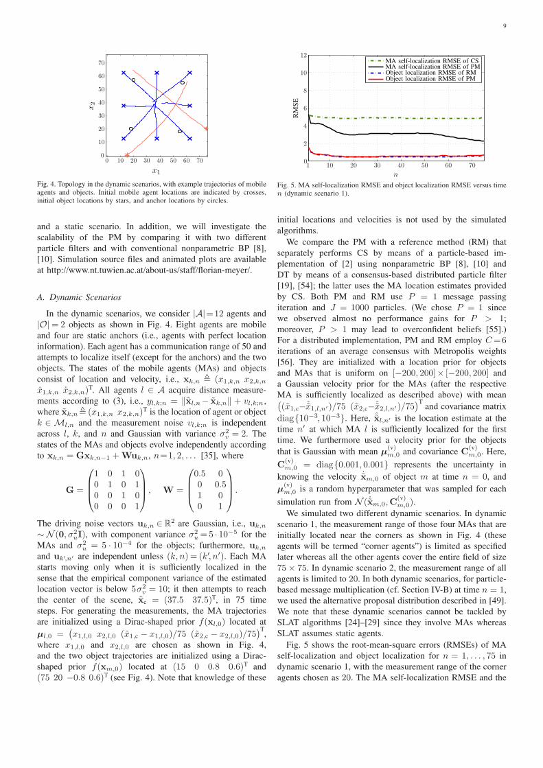
x1

x2

0 10 20 30 40 50 60 700

10

20

30

40

50

60

70

Fig. 4. Topology in the dynamic scenarios, with example trajectories of mobileagents and objects. Initial mobile agent locations are indicated by crosses,initial object locations by stars, and anchor locations by circles.

and a static scenario. In addition, we will investigate the

scalability of the PM by comparing it with two different

particle filters and with conventional nonparametric BP [8],

[10]. Simulation source files and animated plots are available

at http://www.nt.tuwien.ac.at/about-us/staff/florian-meyer/.

A. Dynamic Scenarios

In the dynamic scenarios, we consider |A|=12 agents and

|O|= 2 objects as shown in Fig. 4. Eight agents are mobile

and four are static anchors (i.e., agents with perfect location

information). Each agent has a communication range of 50 and

attempts to localize itself (except for the anchors) and the two

objects. The states of the mobile agents (MAs) and objects

consist of location and velocity, i.e., xk,n , (x1,k,n x2,k,nx1,k,n x2,k,n)

T. All agents l ∈ A acquire distance measure-

ments according to (3), i.e., yl,k;n = ‖xl,n− xk,n‖ + vl,k;n ,

where xk,n, (x1,k,n x2,k,n)T is the location of agent or object

k ∈ Ml,n and the measurement noise vl,k;n is independent

across l, k, and n and Gaussian with variance σ2v = 2. The

states of the MAs and objects evolve independently according

to xk,n = Gxk,n−1 +Wuk,n, n=1, 2, . . . [35], where

G =

1 0 1 00 1 0 10 0 1 00 0 0 1

, W =

0.5 00 0.51 00 1

.

The driving noise vectors uk,n ∈ R2 are Gaussian, i.e., uk,n

∼ N (0, σ2uI), with component variance σ2

u =5 · 10−5 for the

MAs and σ2u = 5 · 10−4 for the objects; furthermore, uk,n

and uk′,n′ are independent unless (k, n) = (k′, n′). Each MA

starts moving only when it is sufficiently localized in the

sense that the empirical component variance of the estimated

location vector is below 5σ2v = 10; it then attempts to reach

the center of the scene, xc = (37.5 37.5)T, in 75 time

steps. For generating the measurements, the MA trajectories

are initialized using a Dirac-shaped prior f(xl,0) located at

µl,0 =(

x1,l,0 x2,l,0 (x1,c − x1,l,0)/75 (x2,c − x2,l,0)/75)T

,

where x1,l,0 and x2,l,0 are chosen as shown in Fig. 4,

and the two object trajectories are initialized using a Dirac-

shaped prior f(xm,0) located at (15 0 0.8 0.6)T and

(75 20 −0.8 0.6)T (see Fig. 4). Note that knowledge of these

n

RM

SE

MA self-localization RMSE of CSMA self-localization RMSE of PMObject localization RMSE of RMObject localization RMSE of PM

1 10 20 30 40 50 60 700

2

4

6

8

10

12

Fig. 5. MA self-localization RMSE and object localization RMSE versus timen (dynamic scenario 1).

initial locations and velocities is not used by the simulated

algorithms.

We compare the PM with a reference method (RM) that

separately performs CS by means of a particle-based im-

plementation of [2] using nonparametric BP [8], [10] and

DT by means of a consensus-based distributed particle filter

[19], [54]; the latter uses the MA location estimates provided

by CS. Both PM and RM use P = 1 message passing

iteration and J = 1000 particles. (We chose P = 1 since

we observed almost no performance gains for P > 1;

moreover, P > 1 may lead to overconfident beliefs [55].)

For a distributed implementation, PM and RM employ C=6iterations of an average consensus with Metropolis weights

[56]. They are initialized with a location prior for objects

and MAs that is uniform on [−200, 200]× [−200, 200] and

a Gaussian velocity prior for the MAs (after the respective

MA is sufficiently localized as described above) with mean(

(x1,c−ˆx1,l,n′)/75 (x2,c−ˆx2,l,n′)/75)T

and covariance matrix

diag{10−3, 10−3}. Here, ˆxl,n′ is the location estimate at the

time n′ at which MA l is sufficiently localized for the first

time. We furthermore used a velocity prior for the objects

that is Gaussian with mean µ(v)m,0 and covariance C

(v)m,0. Here,

C(v)m,0 = diag{0.001, 0.001} represents the uncertainty in

knowing the velocity ˙xm,0 of object m at time n = 0, and

µ(v)m,0 is a random hyperparameter that was sampled for each

simulation run from N ( ˙xm,0,C(v)m,0).

We simulated two different dynamic scenarios. In dynamic

scenario 1, the measurement range of those four MAs that are

initially located near the corners as shown in Fig. 4 (these

agents will be termed “corner agents”) is limited as specified

later whereas all the other agents cover the entire field of size

75× 75. In dynamic scenario 2, the measurement range of all

agents is limited to 20. In both dynamic scenarios, for particle-

based message multiplication (cf. Section IV-B) at time n = 1,

we used the alternative proposal distribution described in [49].

We note that these dynamic scenarios cannot be tackled by

SLAT algorithms [24]–[29] since they involve MAs whereas

SLAT assumes static agents.

Fig. 5 shows the root-mean-square errors (RMSEs) of MA

self-localization and object localization for n = 1, . . . , 75 in

dynamic scenario 1, with the measurement range of the corner

agents chosen as 20. The MA self-localization RMSE and the

10

ρ

RM

SE

MA self-localization RMSE of CSMA self-localization RMSE of PMObject localization RMSE of RMObject localization RMSE of PM

10 12.5 15 17.5 20 22.5 25 27.5 300

2

4

6

8

10

12

Fig. 6. MA self-localization RMSE and object localization RMSE versusmeasurement range ρ of the corner agents (dynamic scenario 1).

n

RM

SE

MA self-localization RMSE of CSMA self-localization RMSE of PMObject localization RMSE of RMObject localization RMSE of PM

1 10 20 30 40 50 60 700

5

10

15

20

25

30

Fig. 7. MA self-localization RMSE and object localization RMSE versus timen (dynamic scenario 2).

object localization RMSE were determined by averaging over

all MAs and all objects, respectively, and over 100 simulation

runs. It is seen that the MA self-localization RMSE of PM

is significantly smaller than that of RM. This is because

with pure CS, the corner agents do not have enough partners

for accurate self-localization, whereas with PM, they can

use their measured distances to the objects to calculate the

messages from the object nodes, φ(p)m→l(xl,n), which support

self-localization. The object localization RMSEs of PM and

RM are very similar at all times. This is because the objects

are always measured by several well-localized agents.

Still in dynamic scenario 1, Fig. 6 shows the MA self-

localization and object localization RMSEs averaged over time

n versus the measurement range ρ of the corner agents. For

small and large ρ, PM performs similarly to RM but for differ-

ent reasons: When ρ is smaller than 12.5, the objects appear

in the measurement regions of the corner agents only with

a very small probability. Thus, at most times, the messages

φ(p)m→l(xl,n) from the object nodes cannot be calculated. For ρ

larger than 25, the corner agents measure three well-localized

agents at time n = 1, and thus they are also able to localize

themselves using pure CS. However, for ρ between 15 and

25, PM significantly outperforms RM (cf. our discussion of

Fig. 5). The object localization RMSEs of PM and RM are

very similar and almost independent of ρ. This is because for

all ρ, the objects are again measured by several well-localized

agents.

Finally, Fig. 7 shows the MA self-localization and object

x1

x2

0 20 40 60 80 1000

20

40

60

80

100

Fig. 8. Topology in the static scenario, with anchor locations (indicated bycircles) and example realizations of non-anchor agent locations (indicated bycrosses) and of object locations (indicated by stars).

localization RMSEs for n = 1, . . . , 75 in dynamic scenario 2

(i.e., the measurement range of all agents is 20). It can be

seen that with both methods, the objects are roughly localized

after a few initial time steps. However, with RM, due to the

limited measurement range, not even a single MA can be

localized. With PM, once meaningful probabilistic information

about the object locations is available, also the self-localization

RMSE decreases and most of the MAs can be localized after

some time. This is possible since the MAs obtain additional

information related to the measured objects. Which MAs are

localized how well and at what times depends on the object

trajectories and varies between the simulation runs.

Summarizing the results displayed in Figs. 5–7, one can

conclude that the MA self-localization performance of PM is

generally much better than that of RM whereas the object

localization performance is not improved. In Section VII-B,

we will present a scenario in which also object localization is

improved. The quantities determining the communication re-

quirements of PM according to Section VI are NC=18000 and

NNBP= 2000. The resulting total communication requirement

per MA and time step is NTOT = 20000 for both dynamic

scenarios. At time n = 1, each MA additionally broadcasts

NAP = 12000 real values for disseminating the alternative

proposal distribution [49]. According to Section VI, the delay

is 9 time slots in both dynamic scenarios. RM has the same

communication requirements and causes the same delay as

PM.

B. Static Scenario

Next, we consider a completely static scenario. This can

be more challenging than the dynamic scenario considered in

the last section, since at the first message passing iterations

the beliefs of all entities can be highly multimodal, and thus

BP algorithms using Gaussian approximations [13], [14] are

typically not suitable for reliable localization. In the simulated

scenario, there are |A|=63 static agents and |O|=50 static

objects. 13 agents are anchors located as depicted in Fig.

8. The 50 remaining agents and the objects are randomly

(uniformly) placed in a field of size 100×100; a realization

of the locations of the non-anchor agents and objects is shown

in Fig. 8. The states of the non-anchor agents and of the

objects are the locations, i.e., xk,n= xk,n= (x1,k,n x2,k,n)T.

11

p

RM

SE

Object localization RMSE of RMAgent self-localization RMSE of RMObject localization RMSE of PMAgent self-localization RMSE of PM

1 2 3 4 5 6 70

2

4

6

8

Fig. 9. Non-anchor agent self-localization RMSE and object localizationRMSE versus message passing iteration index p (static scenario).

Each agent performs distance measurements according to (3)

with a measurement range of 22.5 and a noise variance of

σ2v = 2. The communication range of each agent is 50. The

prior for the non-anchor agents and for the objects is uniform

on [−200, 200]×[−200, 200]. Both PM and RM use J=1000particles and C = 15 average consensus iterations. Since all

agents and objects are static, we simulated only a single time

step. This scenario is similar to that considered in [2] for pure

CS, except that 50 of the agents used in [2] are replaced

by objects and also anchor nodes perform measurements.

For message multiplication, we used the alternative proposal

distribution described in [49].

Fig. 9 shows the localization RMSEs versus the message

passing iteration index p. It is seen that the agent self-

localization performance of PM is significantly better than

that of RM. Again, this is because agents can use messages

φ(p)m→l(xl,n) from well-localized objects to better localize

themselves. Furthermore, also the object localization perfor-

mance of PM is significantly better. This is because with

separate CS and DT, poor self-localization of certain agents

degrades the object localization performance. It is finally seen

that increasing p beyond 5 does not lead to a significant

reduction of the RMSEs.

In this scenario, assuming P = 3, we have NC = 2.70 · 106,

NNBP = 6000, and NTOT = 2.71 ·106. For proposal adaptation,

each non-anchor agent additionally broadcasts NAP = 9.00 ·105 real values [49]. The delay is 54 time slots.

C. Scalability

Finally, we consider again a dynamic scenario and inves-

tigate the scalability of PM for growing network size in

comparison to conventional particle filtering approximating

the classical sequential Bayesian filter. Because this aspect is

not fundamentally related to a distributed implementation, we

consider a centralized scenario where all measurements are

processed at a fusion center. We compare a centralized version

of PM with the sampling importance resampling particle filter

[47] (abbreviated as SPF), the unscented particle filter (UPF)

[57], and a particle implementation of the proposed BP scheme

(6)–(12) using conventional nonparametric belief propagation

(NBP) [8], [10]. Because PM and NBP are centralized, they do

not need a consensus for DT. Both SPF and UPF estimate the

numbers of agents and objects (|A|, |O|)

runti

me

(s)

NBP (J=1000)UPF (J= 5000)NBP (J= 500)UPF (J=1000)PM (J= 5000)SPF (J= 5000)PM (J=1000)SPF (J=1000)

(8, 2) (16, 4) (32, 8) (64, 16) (128, 32)

100

101

102

103

104

Fig. 10. Average runtime versus network size.

total “stacked” state of all MAs and objects, whose dimension

grows with the network size. The state of an MA or object

consists of location and velocity.

We consider mobile networks of increasing size(

|A|, |O|)

= (8, 2), (16, 4), (32, 8), (64, 16), and (128, 32),

where A ⊆ A is the set of MAs. In addition to the MAs and

objects, four anchors are placed at locations (−100 −100)T,

(−100 100)T, (100 −100)T, and (100 100)T. For the MAs

and objects, we use the motion model of Section VII-A

with driving noise variance σ2u = 10−2, and for the agents

(MAs and anchors), we use the measurement model of

Section VII-A with measurement noise variance σ2v = 1. For

generating the measurements, the MA and object trajectories

are initialized as (x1,k,0 x2,k,0 0 0)T, where x1,k,0 and x2,k,0are randomly (uniformly) chosen in a field of size 100×100.

The algorithms are initialized with the initial prior pdf

f(xk,0) = N (µk,0,Ck,0). Here, Ck,0 = diag{10−2, 10−2,10−2, 10−2}, and µk,0 is sampled for each simulation run

from N (xtruek,0,Ck,0), where xtrue

k,0 is the true initial state

used for generating an MA or object trajectory. Since an

informative initial prior is available for all MAs and objects,

we do not use the alternative proposal distribution.

The measurement topology of the network is randomly

determined at each time step as follows: Each MA measures,

with equal probability, one or two randomly chosen anchors

and two randomly chosen MAs or objects. This is done such

that each object is measured by two randomly chosen MAs. In

addition, each object is also measured by one or two randomly

chosen anchors. The sets MAl,n, l ∈ A are symmetric in that

l′∈MAl,n implies l ∈MA

l′,n. Furthermore, the sets Ml,n, l ∈ Aare chosen such that the topology graph that is constituted by

the object measurements performed by the MAs corresponds

to a Hamiltonian cycle, i.e., each MA and object in the graph

is visited exactly once [58]. This ensures that the expected

number of neighbors of each MA and object is independent

of the network size and the network is connected at all times.

PM, SPF, and UPF use J = 1000 and 5000 particles, whereas

NBP uses J = 500 and 1000 particles (J = 5000 would have

resulted in excessive runtimes, due to the quadratic growth of

NBP’s complexity with J). PM and NBP use P = 2 message

passing iterations. We performed 100 simulation runs, each

consisting of 100 time steps.

Fig. 10 shows the average runtime in seconds of all oper-

12

numbers of agents and objects (|A|, |O|)

RM

SE

SPF (J=1000)SPF (J= 5000)NBP (J= 500)NBP (J=1000)PM (J=1000)PM (J= 5000)UPF (J=1000)UPF (J= 5000)

(8, 2) (16, 4) (32, 8) (64, 16) (128, 32)

100

101

Fig. 11. Average localization RMSE versus network size.

ations performed by the fusion center during one time step

versus the network size (|A|, |O|). The runtime was measured

using MATLAB implementations of the algorithms on a single

core of an Intel Xeon X5650 CPU. It is seen that the runtime

of the BP-based methods PM and NBP scales linearly in the

network size, whereas that of the particle filters SPF and UPF

scales polynomially. This polynomial scaling of SPF and UPF

is due to the fact that these filters perform operations involving

matrices whose dimension increases with the network size. For

the same number of particles J , PM always runs faster than

UPF. Furthermore, for the considered parameters and network

sizes, NBP has the highest runtime and SPF the lowest;

however, for larger network sizes, the runtime of SPF and

UPF will exceed that of PM and NBP due to the polynomial

scaling characteristic of SPF and UPF. It is also seen that the

runtime of PM is significantly lower than that of NBP.

Fig. 11 shows the average RMSE, i.e., the average of all MA

self-localization and object localization errors, averaged over

all time steps and simulation runs, versus the network size.

SPF performs poorly since the numbers of particles it uses

are not sufficient to properly represent the high-dimensional

distributions. UPF performs much better; in fact, for J=5000,

it outperforms all the other methods. This is due to a smart

selection of the proposal distribution using the unscented

transform. However, the RMSE of both SPF and UPF grows

with the network size (although for UPF with J =5000, this

is hardly visible in Fig. 11). In contrast, the RMSE of PM

and NBP, which are both based on BP, does not depend on

the network size. The RMSE of PM is only slightly higher

than that of UPF with J=5000. The RMSE of NBP is higher

than that of UPF and PM but considerably lower than that of

SPF; it is reduced when J is increased from 500 to 1000. In

contrast, the RMSE of PM is effectively equal for J = 1000and 5000. Thus, one can conclude that the performance of

PM with J = 1000 cannot be improved upon by increasing

J , and the (small) performance gap between UPF and PM

is caused by the approximate nature of loopy BP. Finally, our

simulations also showed that the performance gap between the

BP-based methods, PM and NBP, and UPF is increased when

the driving noise is increased and/or the measurement noise

is decreased. This is again due to the smart selection of the

proposal distribution in UPF.

These results demonstrate specific advantages of PM over

particle filtering methods. In particular, PM has a very good

performance-complexity tradeoff, and its scaling characteristic

with respect to the network size is only linear.2 For small

networks, this may come at the cost of a slight performance

loss relative to UPF (not, however, relative to SPF, which

performs much worse). For large networks, the performance

of PM can be better than that of UPF, since for a fixed number

of particles, the performance of UPF decreases with increasing

network size (in Fig. 11, this is visible for J = 1000 but only

barely for J = 5000).

An important further advantage of PM applies to dis-

tributed scenarios. Contrary to particle filters, PM facilitates

a distributed implementation since it naturally distributes the

computation effort among the agents. This distribution requires

only communication with neighbor agents, and the commu-

nication cost is typically much smaller than for distributed

particle filters. For example, in the case of the largest simulated

network size of |A| + |O| = 160, for J = 1000, each

agent broadcasts 32000 real values per consensus iteration

to its neighbors. In a distributed implementation of UPF,

for proposal adaptation alone, each agent has to broadcast

to its neighbors a covariance matrix of size 640 × 640 or,

equivalently, 205120 real values per consensus iteration. Ad-

ditional communication is required for other tasks, depending

on the specific distributed particle filtering algorithm used

[18]. Furthermore, for the considered joint CS–DT problem,

UPF is ill-suited to large networks also because it involves

the inversion and Cholesky decomposition of matrices whose

dimension grows with the network size. In large networks,

this may lead to numerical problems on processing units with

limited dynamic range.

VIII. CONCLUSION

We proposed a Bayesian framework and methodology for

distributed sequential localization of cooperative agents and

noncooperative objects in mobile networks, based on recur-

rent measurements between agents and objects and between

different agents. Our work provides a consistent combination

of cooperative self-localization (CS) and distributed object

tracking (DT) for multiple mobile or static agents and objects.

Starting from a factor graph formulation of the joint CS–

DT problem, we developed a particle-based, distributed belief

propagation (BP) message passing algorithm. This algorithm

employs a consensus scheme for a distributed calculation of

the product of the object messages. The proposed integration

of consensus in particle-based BP solves the problem of

accommodating noncooperative network nodes in distributed

BP implementations. Thus, it may also be useful for other

distributed inference problems.

A fundamental advantage of the proposed joint CS–DT

method over both separate CS and DT and simultaneous

localization and tracking (SLAT) is a probabilistic information

transfer between CS and DT. This information transfer allows

2In a distributed implementation, the computational complexity of theconsensus scheme depends on the number of consensus iterations, C, and,in the “consensus–over-weights” case, on the diameter of the communicationgraph, I . Therefore, the scaling might be slightly higher than linear.

13

CS to support DT and vice versa. Our simulations demon-

strated that this principle can result in significant improve-

ments in both agent self-localization and object localization

performance compared to state-of-the-art methods. Further

advantages of our method are its low complexity and its very

good scalability with respect to the network size. The computa-

tion effort is naturally distributed among the agents, using only

a moderate amount of communication between neighboring

agents. We note that the complexity can be reduced further

through an improved proposal distribution calculation that uses

the sigma point BP technique introduced in [14]. Furthermore,

the communication requirements can be reduced through the

use of parametric representations of messages and beliefs [33].

The proposed framework and methodology can be extended

to accommodate additional tasks (i.e., in addition to CS

and DT) involving cooperative agents and/or noncooperative

objects, such as distributed synchronization [39], [40] and

cooperative mapping [59]. Another interesting direction for

future work is an extension to scenarios involving an unknown

number of objects [31], [60] and object-to-measurement asso-

ciation uncertainty [30], [31], [36], [37], [60].

REFERENCES

[1] N. Patwari, J. N. Ash, S. Kyperountas, A. O. Hero III, R. L. Moses, andN. S. Correal, “Locating the nodes: Cooperative localization in wirelesssensor networks,” IEEE Signal Process. Mag., vol. 22, pp. 54–69, Jul.2005.

[2] H. Wymeersch, J. Lien, and M. Z. Win, “Cooperative localization inwireless networks,” Proc. IEEE, vol. 97, pp. 427–450, Feb. 2009.

[3] J. Liu, M. Chu, and J. Reich, “Multitarget tracking in distributed sensornetworks,” IEEE Signal Process. Mag., vol. 24, pp. 36–46, May 2007.

[4] H. Aghajan and A. Cavallaro, Multi-Camera Networks: Principles andApplications. Burlington, MA: Academic Press, 2009.

[5] P. Corke, T. Wark, R. Jurdak, W. Hu, P. Valencia, and D. Moore, “En-vironmental wireless sensor networks,” Proc. IEEE, vol. 98, pp. 1903–1917, Nov. 2010.

[6] F. Bullo, J. Cortes, and S. Martinez, Distributed Control of Robotic Net-works: A Mathematical Approach to Motion Coordination Algorithms.Princeton, NJ: Princeton University Press, 2009.

[7] A. Nayak and I. Stojmenovic, Wireless Sensor and Actuator Networks:Algorithms and Protocols for Scalable Coordination and Data Commu-nication. Hoboken, NJ: Wiley, 2010.

[8] A. T. Ihler, J. W. Fisher, R. L. Moses, and A. S. Willsky, “Nonparametricbelief propagation for self-localization of sensor networks,” IEEE J. Sel.Areas Commun., vol. 23, pp. 809–819, Apr. 2005.

[9] C. Pedersen, T. Pedersen, and B. H. Fleury, “A variational messagepassing algorithm for sensor self-localization in wireless networks,” inProc. IEEE ISIT-11, Saint Petersburg, Russia, pp. 2158–2162, Aug.2011.

[10] J. Lien, J. Ferner, W. Srichavengsup, H. Wymeersch, and M. Z. Win,“A comparison of parametric and sample-based message representationin cooperative localization.” Int. J. Navig. Observ., 2012.

[11] S. Li, M. Hedley, and I. B. Collings, “New efficient indoor cooperativelocalization algorithm with empirical ranging error model,” IEEE J. Sel.Areas Commun., vol. 33, pp. 1407–1417, Jul. 2015.

[12] V. Savic and S. Zazo, “Reducing communication overhead for coopera-tive localization using nonparametric belief propagation,” IEEE WirelessCommun. Lett., vol. 1, pp. 308–311, Aug. 2012.

[13] T. Sathyan and M. Hedley, “Fast and accurate cooperative tracking inwireless networks,” IEEE Trans. Mobile Comput., vol. 12, pp. 1801–1813, Sep. 2013.

[14] F. Meyer, O. Hlinka, and F. Hlawatsch, “Sigma point belief propagation,”IEEE Signal Process. Lett., vol. 21, pp. 145–149, Feb. 2014.

[15] S. Van de Velde, G. Abreu, and H. Steendam, “Improved censoring andNLOS avoidance for wireless localization in dense networks,” IEEE J.Sel. Areas Commun., vol. 33, pp. 2302–2312, Nov. 2015.

[16] A. G. O. Mutambara, Decentralized Estimation and Control for Multi-sensor Systems. Boca Raton, FL, USA: CRC Press, 1998.

[17] T. Vercauteren and X. Wang, “Decentralized sigma-point informationfilters for target tracking in collaborative sensor networks,” IEEE Trans.Signal Process., vol. 53, pp. 2997–3009, Aug. 2005.

[18] O. Hlinka, F. Hlawatsch, and P. M. Djuric, “Distributed particle filteringin agent networks: A survey, classification, and comparison,” IEEESignal Process. Mag., vol. 30, pp. 61–81, Jan. 2013.

[19] S. Farahmand, S. I. Roumeliotis, and G. B. Giannakis, “Set-membershipconstrained particle filter: Distributed adaptation for sensor networks,”IEEE Trans. Signal Process., vol. 59, pp. 4122–4138, Sep. 2011.

[20] O. Hlinka, F. Hlawatsch, and P. M. Djuric, “Consensus-based distributedparticle filtering with distributed proposal adaptation,” IEEE Trans.Signal Process., vol. 62, pp. 3029–3041, Jun. 2014.

[21] M. Uney, D. Clark, and S. Julier, “Distributed fusion of PHD filtersvia exponential mixture densities,” IEEE J. Sel. Topics Signal Process.,vol. 7, pp. 521–531, Jun. 2013.

[22] G. Battistelli, L. Chisci, C. Fantacci, A. Farina, and A. Graziano,“Consensus CPHD filter for distributed multitarget tracking,” IEEE J.Sel. Topics Signal Process., vol. 7, pp. 508–520, Jun. 2013.

[23] C. Fantacci, B.-N. Vo, B.-T. Vo, G. Battistelli, and L. Chisci, “Consensuslabeled random finite set filtering for distributed multi-object tracking.”2015. Available online: http://arxiv.org/abs/1501.01579.

[24] C. Taylor, A. Rahimi, J. Bachrach, H. Shrobe, and A. Grue, “Simultane-ous localization, calibration, and tracking in an ad hoc sensor network,”in Proc. IPSN-06, Nashville, TN, pp. 27–33, Apr. 2006.

[25] V. Savic, H. Wymeersch, and E. Larsson, “Target tracking in confinedenvironments with uncertain sensor positions,” 2015. IEEE Trans. Veh.Technol., to appear.

[26] S. Funiak, C. Guestrin, M. Paskin, and R. Sukthankar, “Distributedlocalization of networked cameras,” in Proc. IPSN-06, Nashville, TN,pp. 34–42, Apr. 2006.

[27] N. Kantas, S. Singh, and A. Doucet, “Distributed maximum likelihoodfor simultaneous self-localization and tracking in sensor networks,”IEEE Trans. Signal Process., vol. 60, pp. 5038–5047, Oct. 2012.

[28] J. Teng, H. Snoussi, C. Richard, and R. Zhou, “Distributed variationalfiltering for simultaneous sensor localization and target tracking inwireless sensor networks,” IEEE Trans. Veh. Technol., vol. 61, pp. 2305–2318, Jun 2012.

[29] M. Uney, B. Mulgrew, and D. Clark, “Cooperative sensor localisationin distributed fusion networks by exploiting non-cooperative targets,” inProc. IEEE SSP-14, Gold Coast, Australia, pp. 516–519, Jun. 2014.

[30] Y. Bar-Shalom, P. Willett, and X. Tian, Tracking and Data Fusion: AHandbook of Algorithms. Storrs, CT: Yaakov Bar-Shalom, 2011.

[31] R. P. S. Mahler, Statistical Multisource-Multitarget Information Fusion.Boston, MA: Artech House, 2007.

[32] F. Meyer, E. Riegler, O. Hlinka, and F. Hlawatsch, “Simultaneousdistributed sensor self-localization and target tracking using belief prop-agation and likelihood consensus,” in Proc. 46th Asilomar Conf. Sig.,Syst., Comp., Pacific Grove, CA, pp. 1212–1216, Nov. 2012.

[33] F. Meyer, F. Hlawatsch, and H. Wymeersch, “Cooperative simultaneouslocalization and tracking (CoSLAT) with reduced complexity and com-munication,” in Proc. IEEE ICASSP-13, Vancouver, Canada, pp. 4484–4488, May 2013.

[34] F. Meyer, H. Wymeersch, M. Fröhle, and F. Hlawatsch, “Distributedestimation with information-seeking control in agent networks,” IEEEJ. Sel. Areas Commun., vol. 33, pp. 2439–2456, Nov. 2015.

[35] X. R. Li and V. P. Jilkov, “Survey of maneuvering target tracking.Part I: Dynamic models,” IEEE Trans. Aerosp. Electron. Syst., vol. 39,pp. 1333–1364, Oct. 2003.

[36] J. L. Williams and R. Lau, “Approximate evaluation of marginal as-sociation probabilities with belief propagation,” IEEE Trans. Aerosp.Electron. Syst., vol. 50, pp. 2942–2959, Oct. 2014.

[37] F. Meyer, P. Braca, P. Willett, and F. Hlawatsch, “Scalable multitargettracking using multiple sensors: A belief propagation approach,” in Proc.FUSION-15, Washington D.C., USA, pp. 1778–1785, Jul. 2015.

[38] Y.-C. Wu, Q. M. Chaudhari, and E. Serpedin, “Clock synchronization ofwireless sensor networks,” IEEE Signal Process. Mag., vol. 28, pp. 124–138, Jan. 2011.

[39] B. Etzlinger, H. Wymeersch, and A. Springer, “Cooperative synchro-nization in wireless networks,” IEEE Trans. Signal Process., vol. 62,pp. 2837–2849, Jun. 2014.

[40] F. Meyer, B. Etzlinger, F. Hlawatsch, and A. Springer, “A distributedparticle-based belief propagation algorithm for cooperative simultaneouslocalization and synchronization,” in Proc. Asilomar Conf. Sig., Syst.,Comput., Pacific Grove, CA, pp. 527–531, Nov. 2013.

[41] S. M. Kay, Fundamentals of Statistical Signal Processing: EstimationTheory. Upper Saddle River, NJ: Prentice-Hall, 1993.

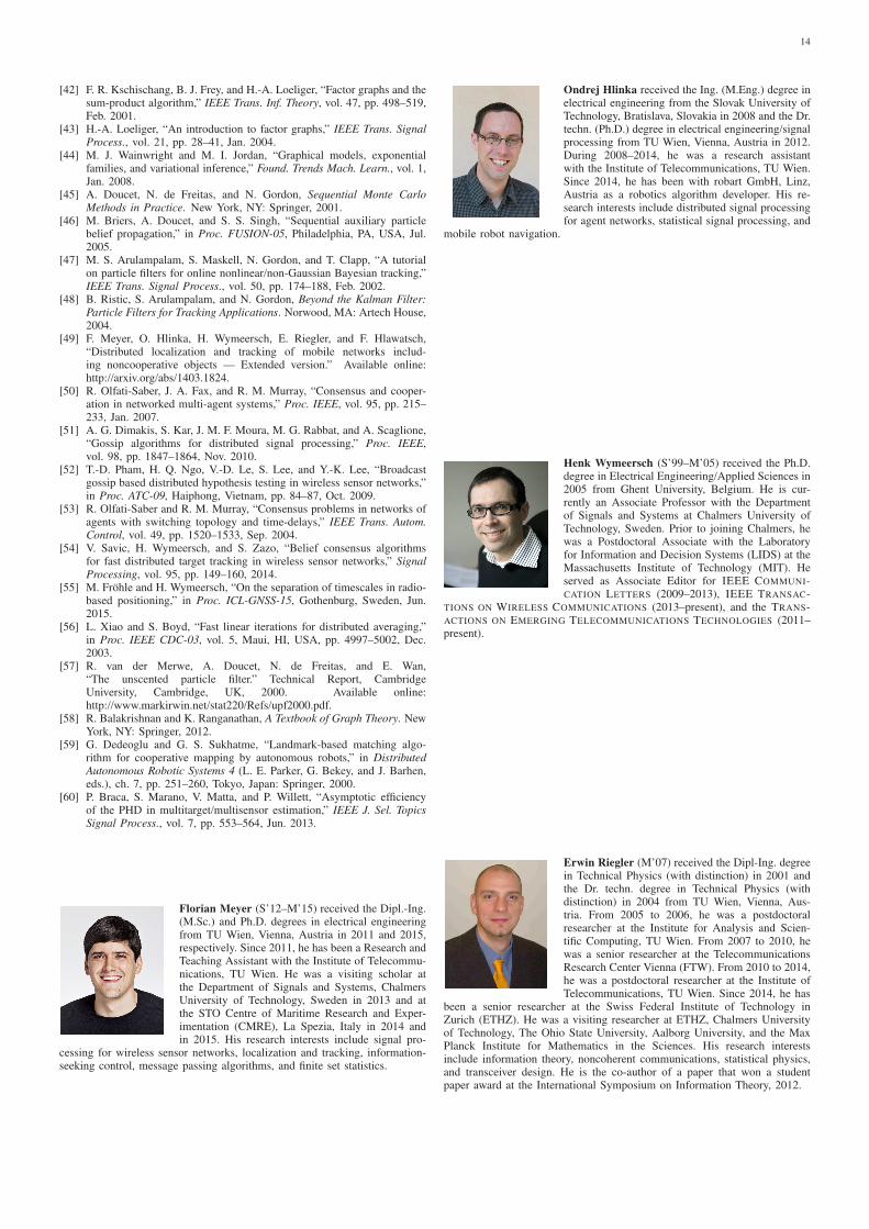
14

[42] F. R. Kschischang, B. J. Frey, and H.-A. Loeliger, “Factor graphs and thesum-product algorithm,” IEEE Trans. Inf. Theory, vol. 47, pp. 498–519,Feb. 2001.

[43] H.-A. Loeliger, “An introduction to factor graphs,” IEEE Trans. SignalProcess., vol. 21, pp. 28–41, Jan. 2004.

[44] M. J. Wainwright and M. I. Jordan, “Graphical models, exponentialfamilies, and variational inference,” Found. Trends Mach. Learn., vol. 1,Jan. 2008.

[45] A. Doucet, N. de Freitas, and N. Gordon, Sequential Monte CarloMethods in Practice. New York, NY: Springer, 2001.

[46] M. Briers, A. Doucet, and S. S. Singh, “Sequential auxiliary particlebelief propagation,” in Proc. FUSION-05, Philadelphia, PA, USA, Jul.2005.

[47] M. S. Arulampalam, S. Maskell, N. Gordon, and T. Clapp, “A tutorialon particle filters for online nonlinear/non-Gaussian Bayesian tracking,”IEEE Trans. Signal Process., vol. 50, pp. 174–188, Feb. 2002.

[48] B. Ristic, S. Arulampalam, and N. Gordon, Beyond the Kalman Filter:Particle Filters for Tracking Applications. Norwood, MA: Artech House,2004.

[49] F. Meyer, O. Hlinka, H. Wymeersch, E. Riegler, and F. Hlawatsch,“Distributed localization and tracking of mobile networks includ-ing noncooperative objects — Extended version.” Available online:http://arxiv.org/abs/1403.1824.

[50] R. Olfati-Saber, J. A. Fax, and R. M. Murray, “Consensus and cooper-ation in networked multi-agent systems,” Proc. IEEE, vol. 95, pp. 215–233, Jan. 2007.

[51] A. G. Dimakis, S. Kar, J. M. F. Moura, M. G. Rabbat, and A. Scaglione,“Gossip algorithms for distributed signal processing,” Proc. IEEE,vol. 98, pp. 1847–1864, Nov. 2010.

[52] T.-D. Pham, H. Q. Ngo, V.-D. Le, S. Lee, and Y.-K. Lee, “Broadcastgossip based distributed hypothesis testing in wireless sensor networks,”in Proc. ATC-09, Haiphong, Vietnam, pp. 84–87, Oct. 2009.

[53] R. Olfati-Saber and R. M. Murray, “Consensus problems in networks ofagents with switching topology and time-delays,” IEEE Trans. Autom.Control, vol. 49, pp. 1520–1533, Sep. 2004.

[54] V. Savic, H. Wymeersch, and S. Zazo, “Belief consensus algorithmsfor fast distributed target tracking in wireless sensor networks,” SignalProcessing, vol. 95, pp. 149–160, 2014.

[55] M. Fröhle and H. Wymeersch, “On the separation of timescales in radio-based positioning,” in Proc. ICL-GNSS-15, Gothenburg, Sweden, Jun.2015.

[56] L. Xiao and S. Boyd, “Fast linear iterations for distributed averaging,”in Proc. IEEE CDC-03, vol. 5, Maui, HI, USA, pp. 4997–5002, Dec.2003.

[57] R. van der Merwe, A. Doucet, N. de Freitas, and E. Wan,“The unscented particle filter.” Technical Report, CambridgeUniversity, Cambridge, UK, 2000. Available online:http://www.markirwin.net/stat220/Refs/upf2000.pdf.

[58] R. Balakrishnan and K. Ranganathan, A Textbook of Graph Theory. NewYork, NY: Springer, 2012.

[59] G. Dedeoglu and G. S. Sukhatme, “Landmark-based matching algo-rithm for cooperative mapping by autonomous robots,” in DistributedAutonomous Robotic Systems 4 (L. E. Parker, G. Bekey, and J. Barhen,eds.), ch. 7, pp. 251–260, Tokyo, Japan: Springer, 2000.

[60] P. Braca, S. Marano, V. Matta, and P. Willett, “Asymptotic efficiencyof the PHD in multitarget/multisensor estimation,” IEEE J. Sel. TopicsSignal Process., vol. 7, pp. 553–564, Jun. 2013.

Florian Meyer (S’12–M’15) received the Dipl.-Ing.(M.Sc.) and Ph.D. degrees in electrical engineeringfrom TU Wien, Vienna, Austria in 2011 and 2015,respectively. Since 2011, he has been a Research andTeaching Assistant with the Institute of Telecommu-nications, TU Wien. He was a visiting scholar atthe Department of Signals and Systems, ChalmersUniversity of Technology, Sweden in 2013 and atthe STO Centre of Maritime Research and Exper-imentation (CMRE), La Spezia, Italy in 2014 andin 2015. His research interests include signal pro-

cessing for wireless sensor networks, localization and tracking, information-seeking control, message passing algorithms, and finite set statistics.

Ondrej Hlinka received the Ing. (M.Eng.) degree inelectrical engineering from the Slovak University ofTechnology, Bratislava, Slovakia in 2008 and the Dr.techn. (Ph.D.) degree in electrical engineering/signalprocessing from TU Wien, Vienna, Austria in 2012.During 2008–2014, he was a research assistantwith the Institute of Telecommunications, TU Wien.Since 2014, he has been with robart GmbH, Linz,Austria as a robotics algorithm developer. His re-search interests include distributed signal processingfor agent networks, statistical signal processing, and

mobile robot navigation.

Henk Wymeersch (S’99–M’05) received the Ph.D.degree in Electrical Engineering/Applied Sciences in2005 from Ghent University, Belgium. He is cur-rently an Associate Professor with the Departmentof Signals and Systems at Chalmers University ofTechnology, Sweden. Prior to joining Chalmers, hewas a Postdoctoral Associate with the Laboratoryfor Information and Decision Systems (LIDS) at theMassachusetts Institute of Technology (MIT). Heserved as Associate Editor for IEEE COMMUNI-CATION LETTERS (2009–2013), IEEE TRANSAC-

TIONS ON WIRELESS COMMUNICATIONS (2013–present), and the TRANS-ACTIONS ON EMERGING TELECOMMUNICATIONS TECHNOLOGIES (2011–present).

Erwin Riegler (M’07) received the Dipl-Ing. degreein Technical Physics (with distinction) in 2001 andthe Dr. techn. degree in Technical Physics (withdistinction) in 2004 from TU Wien, Vienna, Aus-tria. From 2005 to 2006, he was a postdoctoralresearcher at the Institute for Analysis and Scien-tific Computing, TU Wien. From 2007 to 2010, hewas a senior researcher at the TelecommunicationsResearch Center Vienna (FTW). From 2010 to 2014,he was a postdoctoral researcher at the Institute ofTelecommunications, TU Wien. Since 2014, he has

been a senior researcher at the Swiss Federal Institute of Technology inZurich (ETHZ). He was a visiting researcher at ETHZ, Chalmers Universityof Technology, The Ohio State University, Aalborg University, and the MaxPlanck Institute for Mathematics in the Sciences. His research interestsinclude information theory, noncoherent communications, statistical physics,and transceiver design. He is the co-author of a paper that won a studentpaper award at the International Symposium on Information Theory, 2012.

15

Franz Hlawatsch (S’85–M’88–SM’00–F’12) re-ceived the Diplom-Ingenieur, Dr. techn., and Univ.-Dozent (habilitation) degrees in electrical engineer-ing/signal processing from TU Wien, Vienna, Aus-tria in 1983, 1988, and 1996, respectively. Since1983, he has been with the Institute of Telecommuni-cations, TU Wien, where he is currently an AssociateProfessor. During 1991–1992, as a recipient of anErwin Schrödinger Fellowship, he spent a sabbaticalyear with the Department of Electrical Engineering,University of Rhode Island, Kingston, RI, USA.

In 1999, 2000, and 2001, he held one-month Visiting Professor positionswith INP/ENSEEIHT, Toulouse, France and IRCCyN, Nantes, France. He(co)authored a book, three review papers that appeared in the IEEE SIGNAL

PROCESSING MAGAZINE, about 200 refereed scientific papers and bookchapters, and three patents. He coedited three books. His research interestsinclude statistical and compressive signal processing methods and theirapplication to sensor networks and wireless communications.

Prof. Hlawatsch was Technical Program Co-Chair of EUSIPCO 2004and served on the technical committees of numerous IEEE conferences.He was an Associate Editor for the IEEE TRANSACTIONS ON SIGNAL

PROCESSING from 2003 to 2007 and for the IEEE TRANSACTIONS ON

INFORMATION THEORY from 2008 to 2011. From 2004 to 2009, he wasa member of the IEEE SPCOM Technical Committee. He currently servesas an Associate Editor for the IEEE TRANSACTIONS ON SIGNAL AND

INFORMATION PROCESSING OVER NETWORKS. He coauthored papers thatwon an IEEE Signal Processing Society Young Author Best Paper Award anda Best Student Paper Award at IEEE ICASSP 2011.