'D

DTIC ELECTE JAN 2 3 1995

C

DISTRIBUTION STATEMENT A

Appcörad for public ralauwi Distribution Unlimited

FULL LYAPUNOV EXPONENT PLACEMENT IN REENTRY TRAJECTORIES

THESIS

Michael H. Platt, Captain, USAF

AFIT/GA/ENY/95D-03

DEPARTMENT OF THE AIR FORCE

AIR UNIVERSITY

AIR FORCE INSTITUTE OF TECHNOLOGY

I DUO QUALITY IN8PECTBD 9

Wright-Patterson Air Force Base, Ohio

AFIT/GA/ENY/95D-03

FULL LYAPUNOV EXPONENT PLACEMENT IN REENTRY TRAJECTORIES

THESIS

Presented to the Faculty of the School of Engineering

of the Air Force Institute of Technology

Air University

In Partial Fulfillment of the

Requirements for the Degree of

Master of Science in Astronautical Engineering

Michael H. Platt, B.S., MBA. Captain, USAF

December 1995

Aoeessloa For

mis ®S*J>I si mic SAB □ .Unannounced Q Just if icat ior

By__ Distribution/

Availability Codes

Approved for public release; distribution unlimited

I lAvail atid/or JDist , Special

W\

111

The views expressed in this thesis are those of the author and do not reflect the official

policy or position of the Department of Defense or the U.S. government.

Acknowledgments

I would like to thank my advisor, Dr. William Wiesel, Ph.D., for his time, patience

and support. His knowledge, expertise, and humor made this a much more bearable

experience. I would also like to thank my fellow Astro students, Jay Landis, Dave Parrish,

and Greg Schultz for their help with all the little problems that cropped up during this

process. I would like to express my gratitude to my parents for making me believe that

this was possible. And finally, I wish to thank my wife, Auline, for the great editing job on

this thesis. Any errors are mine, not hers. I also offer my thanks to her for putting up

with all my bad moods and long nights throughout the whole AFIT program.

Table of Contents

Page

Acknowledgments u

List of Figures v

List of Tables vn

List of Symbols vin

Abstract lx

I. Introduction 1 1.1 Overview 1

. 1.2 Vehicle Background 1 1.3 Control Background 4 1.4 Principal Accomplishments 5

II. Trajectory Model Design 6

2.1 Assumptions 6 2.2 Equations of Motion 6

2.3 Coefficients of Lift and Drag 10 2.4 Atmospheric Model H 2.5 State Space Version of the Equations of Motion 13 2.6 Trajectory Specifications 15

III. Control Algorithm I7

3.1 Introduction 17 3.2 LyapunovExponents I7

3.3 Algorithm Development I8

IV Implementation of Control Algorithm 24 4.1 Introduction 24 4.2 Trajectory Design Program 24 4.3 Open Loop Value Program 27 4.4 Boundary Value Program 28

V Results 30

5.1 Reentry Trajectory Alternatives 30 5.2 Trajectory Control 41

VI. Conclusions and Recommendations 55 6.1 Conclusions 55 6.2 Recommendations 56

111

Bibliography 59

Appendix A: Lift and Drag on a Cone 60

Appendix B: Equation of Variation 67

Appendix C: A Matrix Equations 69

Appendix D: B Matrix Equations 71

Appendix E: Flowchart for Program DESIGN 72

Appendix F: Flowchart for Program FIRST 73

Appendix G: Flowchart for Program BVP 74

Appendix H: Code Summary 75

Appendix I: Input Files 80

Appendix J: Open Loop Dynamical Direction Vectors 81

Appendix K: Closed Loop Dynamical Direction Vectors 86

Vita 91

IV

List of Figures

Figure Eage

1-1 X-33 Proposed Design Alternative 3 1-2 Typical Launch and Landing Rotation Maneuver 4

2-1 Reference Frames 8 2-2 CDandCL vs Angle of Attack 11

5-1 Case 1: Altitude vs Range Plot 31 5-2 Case 1: Altitude vs Time Plot 31 5-3 Case 1: Speed vs Time Plot 32 5-4 Case 1: Acceleration vs Time Plot 32 5-5 Maximum Lift Angle of Attack: Altitude vs Range Plot 33 5-6 Maximum Lift Angle of Attack: Altitude vs Time Plot 33 5-7 Maximum Lift Angle of Attack: Speed vs Time Plot 33 5-8 Maximum Lift Angle of Attack: Acceleration vs Time 34 5-9 Case 2: Altitude vs Range Plot 34 5-10 Case 2: Altitude vs Time Plot 34 5-11 Case 2: Speed vs Time Plot 35 5-12 Case 2: Acceleration vs Time Plot 35 5-13 Case 3: Altitude vs Range Plot 36 5-14 Case 3: Altitude vs Time Plot 36 5-15 Case 3: Speed vs Time Plot 37 5-16 Case 3: Acceleration vs Time Plot 37 5-17 Case 3: Crossrange vs Time Plot 37 5-18 Case 4: Altitude vs Range Plot 38 5-19 Case 4: Altitude vs Time Plot 38 5-20 Case 4: Speed vs Time Plot 38 5-21 Case 4: Acceleration vs Time Plot 39 5-22 Case 5: Altitude vs Range Plot 39 5-23 Case 5: Altitude vs Time Plot 39 5-24 Case 5: Speed vs Time Plot 40 5-25 Case 5: Acceleration vs Time Plot 40 5-26 Case 5: Crossrange vs Time 40 5-27 Piecemeal Trajectory 48 5-28 Case 1: Gain Plot 49 5-29 Case 2 (0.0-1.0 TU): Gain Plot 51 5-30 Case 3 (0.0-1.0 TU): Gain Plot 52 5-31 Case 4 (0.0-0.25 TU): Gain Plot 52 5-32 Case 5: Gain Plot 53 5-29 Case 2 (0.0-1.0 TU): Gain Plot with Lyapunov Exponents = 0.0 53

5-29 Case 2 (0.0-1.0 TU): Gain Plot with Lyapunov Exponents = -1 thru-6 54 5-29 Case 2 (0.0-1.0 TU): Gain Plot with Lyapunov Exponents = -6.0 54

A-l Vehicle Aerodynamic Model 60

A-2 Coordinate Frames and Important Variables 61 A-3 Surface Element 62

A-4 Change in Momentum 63 A-5 Angle of Attack vs Surface Area 64

B-l Reference Trajectory 67

VI

List of Tables

Table E^

2-1 21 Layer Atmosphere 13

5-1 Initial Conditions 30

5-2 Trajectory Characteristics 41 5-3 Open Loop Lyapunov Exponents 42 5-4 Closed Loop Lyapunov Exponents..... 45 5-5 Open and Closed Loop Lyapunov Exponents for Limited Trajectory Arcs 47

VII

List of Symbols

A aerodynamic vector containing Lift and Drag forces

a angle of attack b atmospheric constant 3.3139xl0"7 (1/m)

% cone half angle C weighting matrix that discourages deviations from the nominal trajectory

D drag D weighting matrix that discourages the use of control

e displacement

(|) latitude

F force vector O state transition matrix

y flight path angle g acceleration vector due to gravity

G gain matrix J linear quadratic regulator cost function

L lift L Lyapunov exponent

\ Lagrange multiplier

LZi lapse rate

m mass n normal vector

P pressure 9 longitude

r radius R gas constant for air

p density of air

a roll S base area of the reentry vehicle Sf weighting matrix that discourages deviations from the nominal trajectory

final conditions

T thrust T temperature

t time u state space control vector

v speed V volume o angular velocity

x state space state vector

v(/ heading £ angle between the projection of the normal vector on the b2,b3 plane and the

b2 axis (see Appendix A)

Z altitude

VIll

AFIT/GA/ENY/95D-03

Abstract

This study investigated the ability to control the chaotic reentry of a Delta Clipper-

like vehicle by setting the values of the initial and final principal dynamical directions as

well as the Lyapunov exponents. A model of the original controlled reentry vehicle was

created through the use of the equations of motion in conjunction with an atmospheric

model. A modified linear quadratic regulator allowed the set up of a boundary value

problem which specified the Lyapunov exponents and determined the gain matrix as a

function of time. The gain matrix can eventually be used in the control system of the

vehicle.

IX

FULL LYAPUNOV EXPONENT PLACEMENT

IN REENTRY TRAJECTORIES

I. INTRODUCTION

1.1 Overview The goal of this paper is to apply the algorithm developed by Wiesel [13]

for specifying Lyapunov exponents, as well as initial and final principal dynamical

directions in a controlled chaotic system. The algorithm makes use of a modified linear

quadratic regulator to set up a boundary value problem. When solved, this yields the

specified Lyapunov exponents (which describe the stability of the system), the initial and

final dynamical directions and the gain matrix over a specified period of time. The gain

matrix can then be used in the control system of the reentry vehicle. The real world system

used to apply this methodology is a Delta Clipper-like launch vehicle. In the second

chapter of this paper, we discuss the development of the dynamics model of the vehicle

reentry trajectory. The third chapter develops the control algorithm. We then detail the

computer code used to implement the model and control algorithm in Chapter 4. Chapter

5 evaluates the results obtained when we attempt to stabilize the chaotic reentry trajectory

of the vehicle model. Finally, Chapter 6 contains conclusions drawn from the results of

this research and recommendations for further study.

1.2 Vehicle Background The Delta Clipper Experimental Launch Vehicle (DCX) was

a Single Stage To Orbit (SSTO), Vertical Take-off, Vertical Landing (VTVL) vehicle

developed by the McDonnell Douglas Corporation under the guidance of the Air Force's

Ballistic Missile Defense Organization (BMDO). This was the first in a series of planned

advanced technology demonstration programs whose eventual goal was to develop

operational SSTO systems. It was hoped that, when fully developed, these systems would

significantly lower the cost per pound to orbit of the U.S. space fleet. The BMDO

designed, fabricated, and flight tested the Delta Clipper vehicle in less than 2 years for

under $70 million. Since then, the BMDO has been directed to deal only with ground-

based missile defense, effectively halting their research in the area of SSTO technology

upon completion of the DCX test program. Currently, the SSTO program is under the

control of NASA, which continues to develop two separate SSTO systems, the X-33 and

the X-34. Of the two vehicles, the X-33 is more likely to resemble the Delta Clipper in

operation and appearance.

A 15 month NASA Concept Definition and Design Phase, initiated in April 1995,

solicited industry teams to compete for the contract to build the X-33. There are three

contractor teams currently involved in this phase. Since the McDonnell Douglas design is

the only one following the VTVL philosophy, we will be using a design similar to theirs

for this project. The final specifications of this version of the X-33 have yet to be

determined, so we will use variations on one of the several proposed designs, seen in

Figure 1-1, as a model for this research.

The main goal of the Delta Clipper program was to create aircraft-like operations

within the space community. The current X-33 vehicle design uses liquid oxygen and

hydrogen for its main engines, and gaseous oxygen and hydrogen for its reaction control

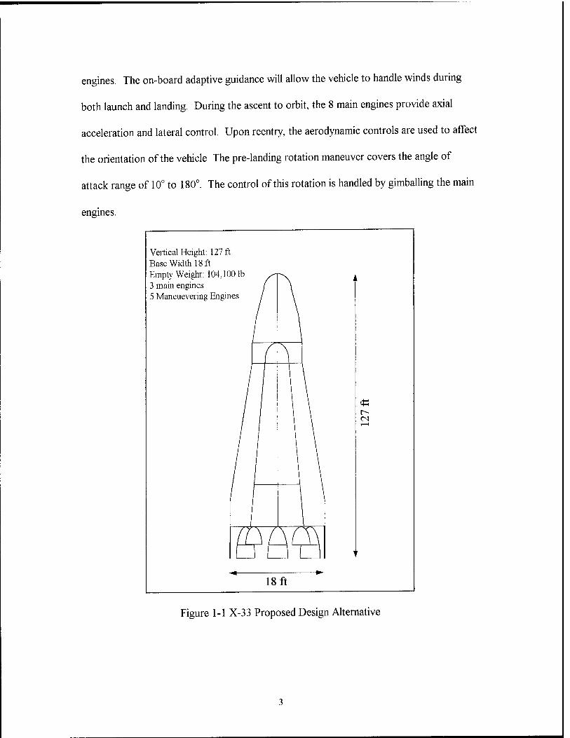
engines. The on-board adaptive guidance will allow the vehicle to handle winds during

both launch and landing. During the ascent to orbit, the 8 main engines provide axial

acceleration and lateral control. Upon reentry, the aerodynamic controls are used to affect

the orientation of the vehicle The pre-landing rotation maneuver covers the angle of

attack range of 10° to 180°. The control of this rotation is handled by gimballing the main

engines.

Vertical Height: 127 ft Base Width 18 ft Empty Weight: 104,1001b 3 main engines 5 Maneuevering Engines

/

i

/ \

} ^OACA □ era

18 ft

Figure 1-1 X-33 Proposed Design Alternative

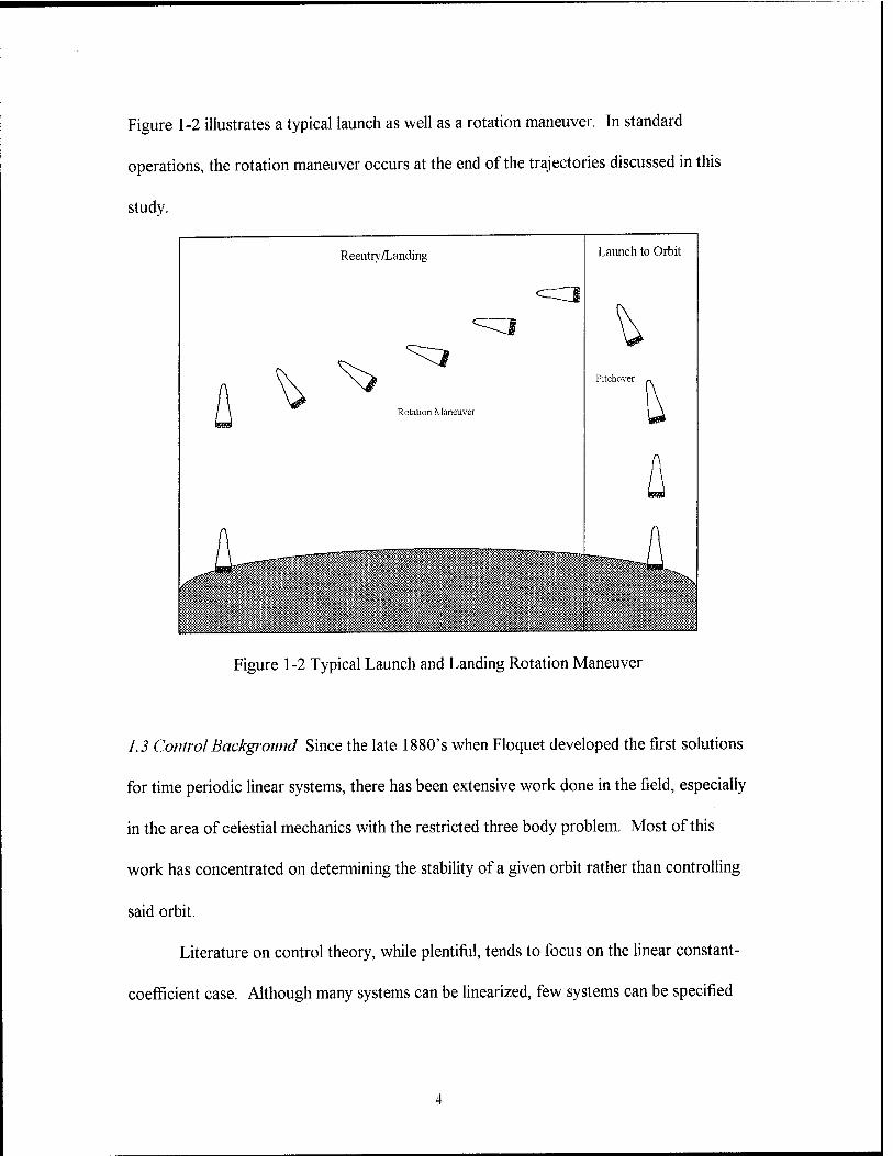
Figure 1-2 illustrates a typical launch as well as a rotation maneuver. In standard

operations, the rotation maneuver occurs at the end of the trajectories discussed in this

study.

Reentry/Landing

^> Rotation Maneuver

Launch to Orbit

Pitchover

Figure 1-2 Typical Launch and Landing Rotation Maneuver

1.3 Control Background Since the late 1880's when Floquet developed the first solutions

for time periodic linear systems, there has been extensive work done in the field, especially

in the area of celestial mechanics with the restricted three body problem. Most of this

work has concentrated on determining the stability of a given orbit rather than controlling

said orbit.

Literature on control theory, while plentiful, tends to focus on the linear constant-

coefficient case. Although many systems can be linearized, few systems can be specified

independent of time, which restricts the use of control. Breakwell et al. [2] dealt with the

control of unstable periodic orbits through use of the Linear Quadratic Regulator. In their

work, Wiesel and Calico [12] designed a method for single pole placement in periodic

systems. Some years later, Wiesel [14] developed a method for dictating the value for a

single pole in a general time-dependent linear system. Recently, Wiesel has extended the

pole placement algorithm to allow full Lyapunov exponent determination in a general

time-dependent linear system. This method also allows specification of the principal

dynamical directions, and will be the main focus of this study.

1.4 Principal Accomplishments The principal accomplishments of this research are:

- Development of a 6 state trajectory design algorithm for a Delta Clipper-like reentry vehicle.

- Successful application of Wiesel's full pole placement algorithm for several example reentry trajectories.

- Discovery of algorithm difficulties in controlling extended trajectory arcs.

- Detection of problems in algorithm calculation of a finite gain matrix.

II. TRAJECTORY MODEL DESIGN

2.1 Assumptions In order to model the reentry trajectory accurately, several general

assumptions must apply. They are as follows.

1. The vehicle specifications will be those listed in Section 1.2.

2. The control variables will be roll and angle of attack.

3. The aerodynamic model, from which the coefficients of drag and lift, CD and CL. are determined, is accurate.

4. The atmospheric model described in Section 2.4 adequately describes the atmosphere through which the reentry vehicle will travel.

5. The 6 dimensional state vector, described in the next section, is sufficient to model the dynamics of the reentry trajectory.

2.2 Equations of Motion The dynamics model we use for the reentry of a vehicle into

the atmosphere is based on a six dimensional state space. Vinh's [11:19-27] formulation

of the equations of motion is used in the following development. We start with the three

parameters which define the motion of the vehicle with respect to the center of the earth:

position vector, f, velocity vector, v, and mass, m. Since the reentry vehicle travels in

the earth centered inertial frame, the position vector of the vehicle, r, is defined by its

magnitude, r, the longitude, 6, and the latitude, ((),. We also define y as the flight path

angle or the angle between the local horizontal plane and the velocity vector, v, and \\J as

the heading or the angle between the local parallel of latitude and the projection of the

velocity vector, v, on the horizontal plane. We now have the six components of the state

space as follows.

r - magnitude of the radius vector 9 - longitude § - latitude v- speed y - flight path angle \\i - heading

At this point, we must determine the equations of motion for the state space

vector. At a given point in time the vehicle is subject to the following force:

F = f + Ä + mg.

f is defined as the force due to thrust, while A is the aerodynamic force, the quantity

mg is the force due to gravity. Since we are assuming an unpowered reentry, T = 0

resulting in the equation,

F = Ä + mg.

Since the vehicle will be moving about within the inertial earth centered frame, we want to

define a rotating frame such that the x axis is aligned with the position vector, the y axis is

in the equatorial frame with positive values toward the direction of motion, and the z axis

completes the right handed system, as seen in Figure 2-1. We can therefore write the

position and velocity vectors as follows:

f = ri (2-0)

v = (vSiny)i + (vCosyCosy)j + (vCosySin\)/)k . (2-1)

z z

/v / Y

\ ! x

Figure 2-1. - Reference Frames

We know that in the rotating system the following definition of velocity is valid,

- df - _ v = — = co x r,

dt

with the value of w being defined as :

co = (Sin<[> —) l - (—) j + (Cos(|> — )k. dt dt dt

Since we know that

dr .dr.r ,di. — = (—)i +(—)r, dt V vdt'

(2-2)

where

di - r .„ ,d9- ,d(j> - — = © x i = (Coscp—)j + (-J)k, dt dt dt

we can equate equations 2-1 and 2-2 to get the following three equations of motion:

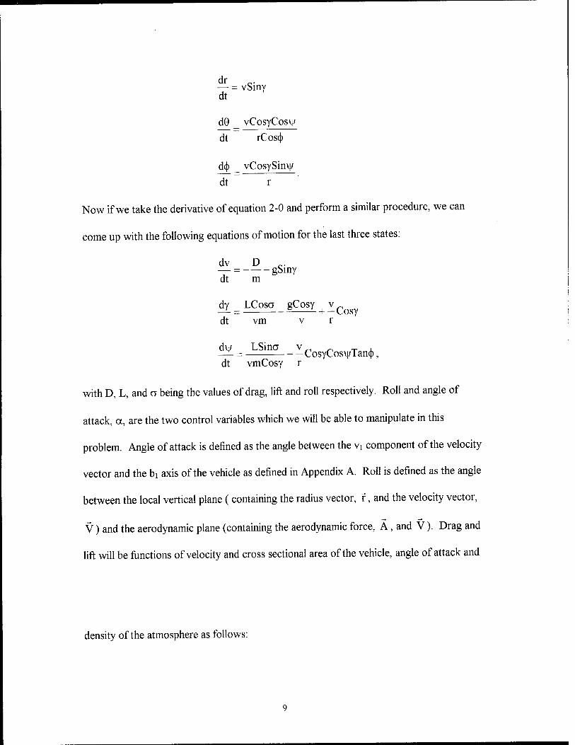
— = vSiny dt

d9 _ vCosyCosy

dt rCos(()

d(|) _ vCosySin\|/

dt~~ r '

Now if we take the derivative of equation 2-0 and perform a similar procedure, we can

come up with the following equations of motion for the last three states:

dv D _. — = gSiny dt m

dy = LCosa_gCosy + vCosY

dt vm v r

— = CosyCosvj/Tantj), dt vmCosy r

with D, L, and a being the values of drag, lift and roll respectively. Roll and angle of

attack, a, are the two control variables which we will be able to manipulate in this

problem. Angle of attack is defined as the angle between the vi component of the velocity

vector and the bi axis of the vehicle as defined in Appendix A. Roll is defined as the angle

between the local vertical plane ( containing the radius vector, f, and the velocity vector,

V) and the aerodynamic plane (containing the aerodynamic force, A, and V). Drag and

lift will be functions of velocity and cross sectional area of the vehicle, angle of attack and

density of the atmosphere as follows:

D = pSCD(a)V2

L pSCL(a)V2

The angle of attack can be used to determine the coefficients of drag and lift, Cd and CL.

The method of calculating the coefficients of lift and drag is contained in the next section.

2.3 Coefficients of Lift and Drag In order to determine the coefficients of lift and drag,

we must first determine the shape of the reentry vehicle. Using the vehicle shown in

Figure 1-1, we can extrapolate a model for the vehicle which is represented by a cone with

an 8° cone half angle, %, and a base diameter of 12.19 meters (see Figure A-l). Appendix

A contains the derivation of the following equations which allow us to determine CD and

CL based upon the angle of attack of the vehicle.

Tan(x)^

CDA = L2{

2[Sin(x)Cos(a) + Cos(C)Cos(x)Sin(a)]2

x [Sin(x)Cos(a) + Cos(x)Cos(QSin(a)]

Cos(x) Mc

CLA = L2{

2[Sin(x)Cos(a) + Cos(QCos(x)Sin(a)] 2 Tan(x)

Cos(x)

where C, =

x (Sin(x)Sin(a) - Cos(x)Cos(C)Cos(a)]

K when a < x I Cos'[-Tan(x)Ctn(a)] when a>xj

dC

10

These equations allow us to calculate a CD and a CL for any angle of attack if we

are given a cone half angle, C,. For the 8 degree cone half angle of our vehicle, this

converts to the graph of CD and CL versus angle of attack in Figure 2-2.

10 20 30 40 50 60 Angle of Attack (degrees)

70 80 90

Figure 2-2 CL and CD vs Angle of Attack

2.4 Atmospheric model Once the coefficients of lift and drag have been determined, it is

necessary to find the density of the atmosphere at the altitude of the reentry vehicle. We

use the method developed by Regan [10:21-45] which utilizes a linear model of the

atmosphere, divided into 21 discrete sections from 0 to 700 km. The model assumes

11

several characteristics of the atmosphere including thermodynamic fluid behavior and

equilibrium under both pressure and gravitational forces. These two characteristics result

in the following equations:

dP

where

dZ -Pg

PV=R* T.

g = acceleration due to gravity P = pressure R = gas constant for air p = density of air T = temperature V = volume

These equations lead to an atmosphere with several break points indicating

changes in the slope of density curves. Table 2-1 gives the base parameters and the lapse

rate which defines the changes in the respective regions. To determine the actual density

at an altitude we use the following equations:

If Lapse Rate = 0

P = Pi exp

If Lapse Rate *0

go(Z-Zi)'

RT Mj

i-f(z-z.)

p = pi

fi \

v iMi. (Z-Zj) + 1

80

RLZi,<

RLZi . , TM

So 1+b -^--Z,

expi g0b (Z-Zi)

where i indicates the value at the bottom of the respective region listed in Table 2-1.

12

This model represents a standard atmosphere. It does not take into account any daily

variations or changes due to unpredicted solar activity. It also ignores the effects of

atmospheric winds on the pressure in a given area.

Layer Index Geometric Altitude (km)

Molecular Temperature (K)

Lapse Rate K/km

0 0.0 288.15 -6.5

1 11.0102 216.65 0.0

2 20.0631 216.65 +1.0

3 32.1619 228.65 +2.8

4 47.3501 270.65 0.0

5 51.4125 270.65 -2.8

6 71.8020 214.65 -2.0

7 86.0 186.10 +1.7

8 100.0 210.65 +5.0

9 110.0 260.65 + 10.0

10 120.0 360.65 +20.0

11 150.0 960.65 +15.0

12 160.0 1110.65 +10.0 13 170.0 1210.65 +7.0 14 190.0 1350.65 +5.0 15 230.0 1550.65 +4.0 16 300.0 1830.65 +3.3

17 400.0 2160.65 +2.6 18 500.0 2420.65 + 1.7 19 600.0 2590.65 +1.1 20 700.0 2700.65

TABLE 2-1 21 Layer Atmosphere

2.5 State Space Version of the Equations of Motion The equations of motion for a

nonlinear time-dependent system are usually written in the following form:

X=f(X,U,t).

13

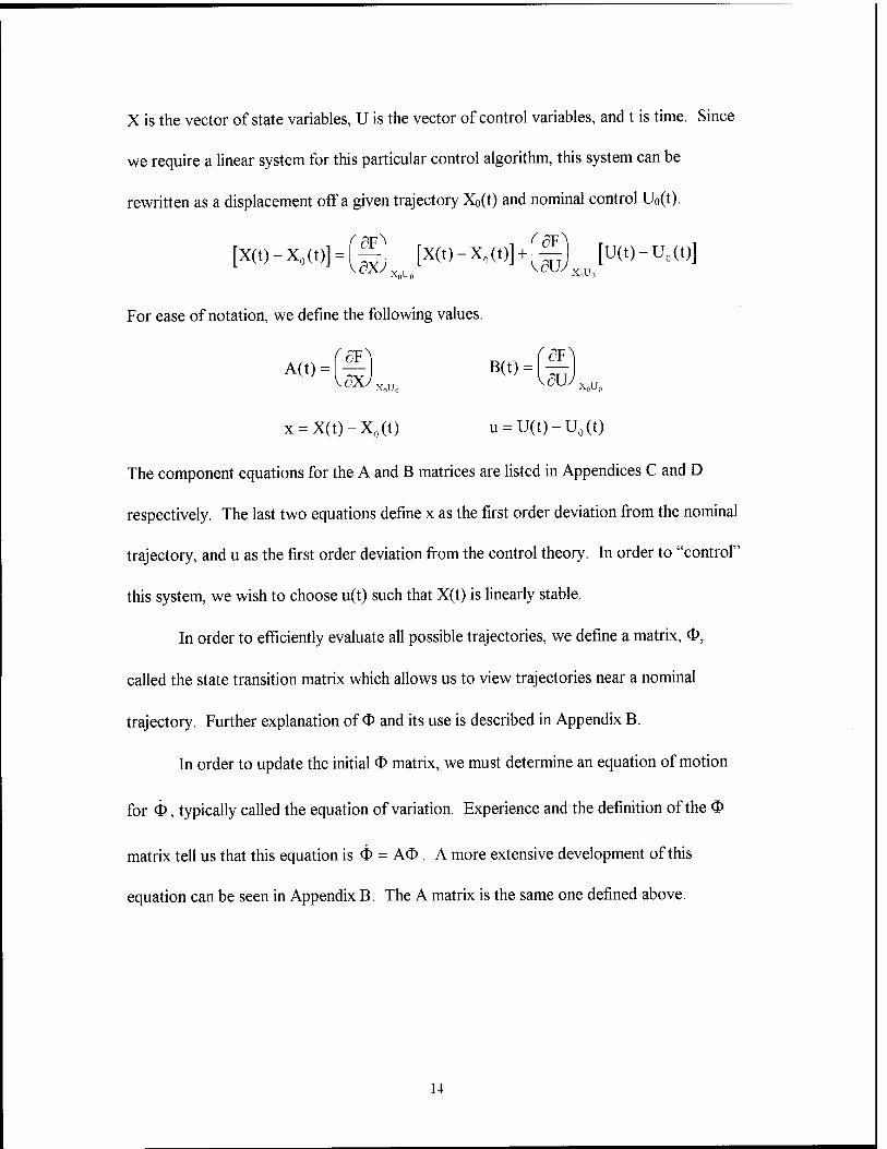
X is the vector of state variables, U is the vector of control variables, and t is time. Since

we require a linear system for this particular control algorithm, this system can be

rewritten as a displacement off a given trajectory X0(t) and nominal control U0(t).

[X(t)-X0(f)] = fi|] [X(t)-X0(t)] + f^l [U(t)-U0(t)]

For ease of notation, we define the following values.

mjm B(„=(f)

x = X(t)-X0(t) u = U(t)-U0(t)

The component equations for the A and B matrices are listed in Appendices C and D

respectively. The last two equations define x as the first order deviation from the nominal

trajectory, and u as the first order deviation from the control theory. In order to "control"

this system, we wish to choose u(t) such that X(t) is linearly stable.

In order to efficiently evaluate all possible trajectories, we define a matrix, O,

called the state transition matrix which allows us to view trajectories near a nominal

trajectory. Further explanation of $ and its use is described in Appendix B.

In order to update the initial <J> matrix, we must determine an equation of motion

for Ö, typically called the equation of variation. Experience and the definition of the O

matrix tell us that this equation is Ö = A® . A more extensive development of this

equation can be seen in Appendix B. The A matrix is the same one defined above.

14

2.6 Trajectory Specifications With the equations of motion determined, we are able to

propagate the vehicle through its trajectory from any initial condition. In order to

accomplish the entire integration, we must first design a trajectory. Basically, this involves

setting the initial conditions and the control law based on the probable reentry point and

the characteristics of the vehicle. Since in this example we are using a DCX-like launch

vehicle, we assume that we will be able to control both angle of attack and roll using the

control system of the reentry vehicle. This allows us to specify these two control variables

at any given time. The control law we will be using is very simple; the law checks to see if

the vehicle is at a pull-up point. This is the point in the trajectory where the aerodynamic

forces cause enough lift on the vehicle to cause it to increase in altitude. If it is, from that

point on the angle of attack is adjusted so that it produces just enough lift to keep the

vehicle in level flight. The roll is maintained at its initial value. We look at five trajectories

in order to fully validate the flexibility of the control algorithm. The first trajectory is a

ballistic trajectory with the vehicle reentering with both control variables, roll and angle of

attack, set equal to zero.

The second trajectory has roll set equal to zero for the entire flight, while the pitch

is maintained at the initial value until the vehicle reaches the point at which it begins to pull

up. At this point the angle of attack is adjusted so that the vehicle maintains a level flight

for as long as possible. The initial angle of attack will be selected to maximize the flight

time. This trajectory is designed to give us the longest possible time at a higher altitude,

thereby avoiding the aerodynamic forces the vehicle is subject to at lower altitudes. Since

the only way the vehicle can maintain level altitude is by generating lift, it experiences

15

some aerodynamic forces. However, staying higher until its velocity has decreased reduces

the overall negative effects of reentry such as heating and deceleration.

The third trajectory is identical to the second trajectory, except the roll is set a

specific non-zero value for the entire reentry. This maintains the benefit of less

aerodynamic forces while allowing the vehicle to adjust for any cross range error which

might be present. The fourth trajectory has zero initial angle of attack and 0.5 radian

initial roll. This allows us to determine how the algorithm handles roll with no angle of

attack. The final trajectory has no initial roll and a 1.5 radian initial angle of attack. This

allows us to evaluate how the algorithm will handle large angles of attack.

With the trajectory designed, we will iterate the state vector and the O matrix

through the entire flight. The trajectory is terminated when the radius drops below the

radius of the earth. Upon termination of the trajectory, the final d> matrix is used to

determine the stability of the trajectory (see next section). All these trajectories are

simplistic, in that they do not contain any post-reentry maneuvering independent of the

control law we have established for angle of attack. This simplicity is due to the fact that

the trajectories are being used only to observe the control algorithm discussed in the next

section and therefore represent certain extremes of the possible trajectories.

16

III. Control Algorithm

3.1 Introduction Control theory often deals with the control of constant coefficient

linear systems. Some extensive work has also been done with time periodic systems.

However, Wiesel [14] has recently developed a modal decomposition for the general time-

dependent system and formulated a method for moving a single pole to any desired

location. A later Wiesel paper [13] details a method for placing all the control system's

Lyapunov exponents and dynamical directions. The general features of this control

method are detailed below.

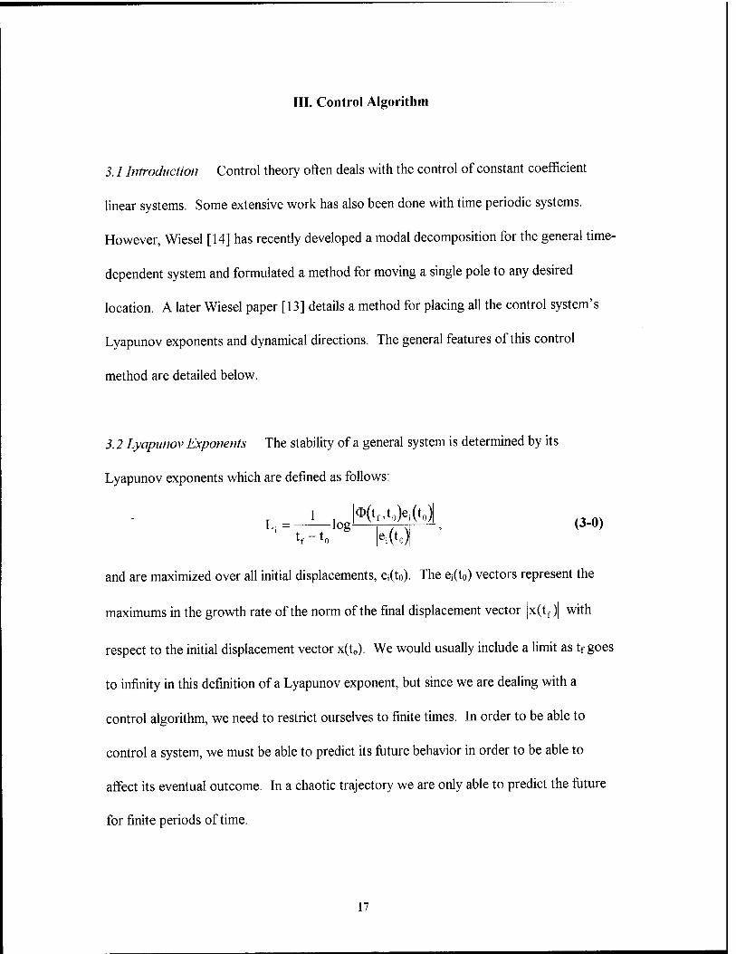
3.2 Lyapunov Exponents The stability of a general system is determined by its

Lyapunov exponents which are defined as follows:

Li=^logl*('.ffJ, ,3-0)

and are maximized over all initial displacements, e;(t0). The e;(to) vectors represent the

maximums in the growth rate of the norm of the final displacement vector |x(tf )| with

respect to the initial displacement vector x(t0). We would usually include a limit as tf goes

to infinity in this definition of a Lyapunov exponent, but since we are dealing with a

control algorithm, we need to restrict ourselves to finite times. In order to be able to

control a system, we must be able to predict its future behavior in order to be able to

affect its eventual outcome. In a chaotic trajectory we are only able to predict the future

for finite periods of time.

17

We must constrain maximization described earlier in order to avoid a large initial

displacement resulting in a final displacement too large to handle. To accomplish this, we

simply assume the magnitude of the principal dynamical direction vectors, u and v, to be

unity, suchthat:

h(to)| = H = i = K(tf)| = |u|.

3.3 Algorithm Development In their work, Bryson and Ho [3] develop the concept of a

Linear Quadratic Regulator (LQR) used below. We start with the following formulation

of the system developed from the above equations:

x = A(t)x + B(t)u. (3-1)

We then create a performance index which we will attempt to minimize. In normal

LQR's, the matrices Sf, C, and D are positive definite and discourage deviations from the

nominal trajectory final conditions, deviations from the nominal trajectory and the use of

control, respectively. We are modifying the LQR so that we are actually specifying the

Lyapunov exponents of the system, therefore we are no longer able to ensure that these

matrices, especially Sf, will be positive definite.

tf

J = -xfTSfxf+-j(xTCx + uTDu)dt (3-2)

2 2t„

By manipulating equation 3-1, we are able to incorporate Lagrange multipliers creating

the following equation:

1 1 tf

J' = -xfTSfxf+-J(xTCx + uTDu + 2A,T[Ax + Bu-x])dt.

18

If we integrate thex by parts we get

J' = -xfTSfxf-^Tx|;;+-j(xTCx + uTDu + 2^T[Ax + Bu] + 2^Tx)dt.

Since we are trying to minimize J', we must zero the first variation of J', 5J' = 0,

which, along with equation 3-1, results in the following equations:

x = A(t)x + B(t)u (3-3)

Ä = -ATA-CTx (3-4)

u = -D"'BTX (3-5)

A,f=SfTxf. (3-6)

For this particular problem, we ignore the C matrix. Rather than simply discouraging the

deviation from the nominal trajectory, we will actually specify the stable Lyapunov

exponents for the closed loop system. This alters equation 3-4 into the equation

X = -ATl. (3-7)

Combining equations 3-3 and 3-5 leads to another formulation of the derivative of the

state vector:

x^Ax-BD-'B1^. (3-8)

We now want to solve the above equations as a boundary value problem. In most

cases, we have initial conditions x(t0) and the freedom to choose one more set of

boundary values. The logical choice is equation 3-6, which is then used in its general

form, A, = Sx, along with equation 3-7 to yield

Sx + Sx = -ATSx,

which when combined with equation 3-8 results in the next equation,

19

S = SBD 'BTS-ATS-SA.

This equation is called the matrix Ricatti Differential equation and can be propagated

independently of the closed loop linear system and the Lagrange multiplier equations.

Since we know the final value, Sf, we are able to use the Ricatti equation to sweep back

through the trajectory and determine S0. This in turn yields X(t0) from equation 3-6 and

the initial conditions. Now equations 3-7 and, subsequently, 3-3 can be integrated

forward through the designated period of time. This algorithm is called the dual sweep

method. It also allows us to rewrite equation 3-4 in the following form:

x = (A-BD"'BTS)x

Using equation 3-5, we define the following value as the gain matrix,

G(t) = -D"'BTS, which allows us to write equation 3-3 in this form:

x = (A + BG)x.

If we are able to determine the values of the G matrix with respect to time, these values

can be input into the reentry vehicle's control system allowing the vehicle to actually fly

the specified reentry trajectory.

Previously, we assumed that the final value of S was known. Instead of simply

defining how much we want the final conditions to deviate from the nominal final

conditions, we would rather establish stability conditions on the dynamics of the system.

One measure of the stability of a given path of the trajectory is its Lyapunov exponents. It

is a fairly simple exercise to determine the open loop Lyapunov exponents. Since we

know the open loop system follows the restriction,

<t> = AO ,

20

where Ox (t0) = I, and I is the identity matrix. By decomposing the Ox matrix at t=tf,

we are left with singular vectors u and v and diagonal matrix W of the form

(Dx(tf) = uWvT.

The vector v is an orthonormal vector that gives the directions that the initial

conditions of the given trajectory differ from the initial conditions of the reference

trajectory in state space on a unit sphere at time t=t0 • This matrix propagates through the

trajectory in the directions on the ellipsoid defined by the orthonormal u matrix at time

t=tf. The values of the components in the diagonal W matrix are the axis lengths of the

ellipsoid at t=tf. The Lyapunov exponents are then defined as a variation of equation 3-0

or

—log(wi). tf -t0

The above equations are valid for both the open and closed loop cases. Since we

want to be able to specify what the closed loop Lyapunov exponents will be, we will

simply set the closed loop principal dynamical directions equal to the open loop values

such that, Uo=Uc and v0=vc. We know the open loop Lyapunov exponents, L;.0, and we

will specify the closed loop Lypunov exponents, Lj,c. Using equations 3-7 and 3-8 and

taking the partial derivatives with respect to initial conditions, x(t0), we get the following

result:

A<j> -AO^-BC^O, (3-9) dt x'c

21

Aa>. =-AT

<D,, (3-io) dt x

where Oxc = ck(t)/3x(t0)

and ®}=dX(t)/dx(t0)

These equations then form a linear boundary value problem. To solve the problem for the

values of ®x(t0), we must integrate equations once to get the open loop solution and then

(order)2 or 36 times to get the numerical partial derivatives, dOx c (tf )/5$x (t0). Once we

have these values, one iteration of the Newton Rhapson method,

"^x.c(tf)n_1

<Mt<>) 9*x(to)

(d>xC(tf)-Ox0(tf)).

will yield the value for Ox(t0) for the given value of Ox c (tf).

Previously we implied that by specifying the closed loop Lyapunov exponents, we

were in effect eliminating the need to define an Sf matrix. Now we can prove this

assumption is valid. Since we are able to calculate the value of O^ (t0), using equation

3-6 and the initial conditions give us the values of S0, we can then integrate forward using

the Ricatti equation to get Sf. So, Sf is implicitly determined by our choice of the

Lyapunov exponents and the principal dynamical directions. Recall that since we are using

a modified LQR, there is not guarantee that Sf will be positive definite as it would be in a

normal LQR.

22

IV. Implementation of the Control Algorithm

4.1 Introduction There are basically three programs which are required to implement

Wiesel's control algorithm. The trajectory design program, DESIGN, the open loop

calculation program, FIRST, and the boundary value program, BVP. In order to avoid

problems which arose in trying to decompose matrices and solve linear equations that

were written in terms of metric units, most units in the code are handled in non-

dimensional units. These units which we will call Distance Units (DUs) and Time Units

(TUs) are defined below.

1DU = 6378.145km

ITU =806.8118744 sec

1^ = 7.90536828^1 TU sec

The only subroutine which uses metric units is the atmospheric model which is part of the

dynamics model and will be described below. The flow chart for the three different

programs can be found in Appendices E, F, and G. The main characteristics of the

programs and subroutines listed below can be found in Appendix H and the input files

required by each program can be found in Appendix I.

4.2 Trajectory Design Program In order to test the control algorithm, we must first set

up the computer model of the trajectory dynamics. The trajectory design program,

DESIGN, accepts the initial conditions of the state vector, control variables, and other

miscellaneous parameters from an input file. It then calls a routine developed by Dr

Wiesel, called AERO, which accepts the angle of attack of the vehicle, uses a reference

23

table derived by the method detailed in Appendix A, and outputs the coefficients of drag

and lift, CD and CL, and derivatives of these values with respect to angle of attack. At this

point, DESIGN provides the maximum lift angle of attack, causing AERO to output the

maximum lift CL and Co-

The code then initializes an integration routine called HAMING. This subroutine

is an ordinary differential equations integrator using a fourth-order predictor-corrector

algorithm. The code saves the last four values of the state vector and O matrix and uses

these to determine the predicted value of the state vector and the O matrix. This

predicted value is then corrected using the equations of motion and the A matrix to find

the new value of the state vector and <J> matrix. Since we only provide the trajectory

design program with one set of initial conditions rather than the four required by the

Haming subroutine, an algorithm called a Picard iteration is used to find the other three.

This process is not used for the entire iteration since it is much slower than the Haming

algorithm. Within the HAMING routine, a subroutine called PHIRHS is implemented.

PHIRHS calls a dynamics routine and uses the output of this to calculate the equations of

motion for the state vector and <£ matrix which HAMING in turn uses to propagate the

orbit.

The dynamics subroutine that PHIRHS calls is named DYNAM. After defining

some initial parameters, this subroutine calls the AERO subroutine described earlier and

determines the CL and CD for the current angle of attack. The routine then checks to see if

the vehicle is in a pull up maneuver. If it is, DYNAM determines the new CL and CD, if it

is not, the program checks to see if the vehicle is within an altitude range for which the

24

atmospheric model is valid. If the vehicle is outside the acceptable altitude range (0-

700km), the code outputs that the model is not valid. If the vehicle is within the

acceptable range, DYNAM calls the atmospheric model subroutine called ATM. This

routine first converts the altitude and density at sea level to metric units. It then

determines which of the 21 layers of the atmosphere the vehicle is in and calculates the

density, pressure and temperature at the current altitude. These values are converted back

to non-dimensional units and returned to DYNAM. The code determines the current

values for the equations of motion for the state vector and the values of the A and B

matrices.

Once HAMTNG has been initialized, it is run a pre-selected number of times. After

each run of HAMING, the program checks to see if the vehicle has reached the point

where it is starting to pull up (i.e. an increase in altitude). If it has, the CL is adjusted so

that the vehicle remains in level flight; HAMING is reinitialized; and a flag is initiated to

ensure that CL will be continuously adjusted for level flight. If a pull up has not occurred

yet, the iteration continues.

At this juncture the program checks for whether the vehicle has dropped below a

minimum height signifying impact. The impact value can be set at any value (ie sea level

or some point above to represent the point at which a Delta Clipper-like vehicle would

perform its rotation to vertical maneuver prior to landing). After this check, the necessary

variables are written to several output files. The trajectory design program creates

numerous files which can be used to graph different combinations of the state variables. It

also creates an output file called FIRST.IN which is used in the next program, FIRST.

25

This file contains the number of iterations of HAMING that have been accomplished as

well as the initial conditions and parameters that were input to DESIGN. Three other files

that will be used in both FIRST and BVP are created as well. These files, CONTROL,

CONTROL2.0UT, and CONTROL3.0UT, contain a control history of the trajectory,

including the time, pitch, roll, CD, and CL values at each iteration of HAMING.

4.3 Open Loop Value Program Once the trajectory has been designed, we are able to

implement the control algorithm. The first program that accomplishes this is appropriately

called FIRST. This program accepts the output of DESIGN, and iterates through the

trajectory, updating the state vector and the O matrix. It then uses the program

SVDCMP, which performs a singular value decomposition of the <D matrix, to get the

orthonormal dynamical direction vectors, u and v and the W matrix. From the W matrix,

it calculates the open loop Lyapunov exponents. Since the next program implements the

boundary value portion of the control algorithm, FIRST outputs all the initial conditions

and parameters to a file called BVP. IN along with two copies of the open loop Lyapunov

exponents , the open loop u and the open loop v vectors. Two copies are written to this

file because the input file for the boundary value program, BVP, requires both the open

loop values and the required closed loop values. Since the closed loop u and v vectors

will be set equal to their open loop values for our purposes, it is convenient to simply edit

the BVP.IN file prior to running BVP so that the second Lyapunov exponents are our

desired closed loop values.

26

4.3 Boundary Value Problem Program The program BVP needs both the open loop

Lyapunov exponents and principal directions, as well as the desired closed loop Lyapunov

exponents and principal directions in order to set up the boundary value problem so, as

stated above, we now edit BVP.IN to include the desired closed loop values of the

Lyapunov exponents. Once this is done, BVP accepts the input file BVP.IN and

constructs a desired closed loop O matrix based on the closed loop u and v vectors and

the Lyapunov exponents. The program initializes both the <t» matrix and another matrix,

called the O Lagrangian matrix which is made up of the Lagrangian multipliers. It iterates

through the trajectory calculating the open loop O and O Lagrangian values. The

program then iterates through the trajectory (order)2 or 36 times to construct the O

Lyapunov numerical partials. This is accomplished by adding a delta value to the initial O

Lagrangian element and determining the final O element after the trajectory is integrated.

The value of the final element without perturbation is subtracted from the value with

perturbation and the difference is divided by the delta value in the following manner.

PO O -O *-' ^*^ Pprfnt+ipH I Pcttuibed Unpereturbed

50x delta

From these partials, the program calculates the final <f> Lagrangian matrix. This is

done by solving the following matrix equation of the partials (Basis), the O Lagrangian

matrix and the error matrix.

(Basis)(<D?J = E

Where E = 0DeiS).rerf - ^ Unperturbed

27

This results in a <$>x at t=t0. The code iterates through the trajectory one final time to

validate the solution. During this iteration, the gain matrix is written to an output file

along with the time and the value of the state variables at that point in time. After this run

through the trajectory, the achieved <X> matrix and the closed loop Lyapunov exponents

and u and v vectors are output.

28

V. RESULTS

5.1 Reentry Trajectory Alternatives For our purposes, all the trajectories will start with

the same initial conditions listed below in Table 5-1. The only values that will be changed

are the initial control variables, angle of attack and roll. In order to test the control

algorithm on the extremes of possible trajectories, we must first determine what those

extremes are.

Radius 6528.145 km Longitude 0.000 rad Latitude 0.000 rad Velocity 7.807 km/sec2

Flight path Angle -0.085 rad Heading 0.000 rad Mass of the Vehicle 45994.740 kg

Table 5-1 Initial Conditions

It would make sense that the ballistic trajectory (Case 1), in which initial roll and

angle of attack are zero, would result in a short trajectory with a high deceleration. From

Figure 5-1, we can see that the output of the DESIGN program seems to agree with this.

Since the initial roll and angle of attack of zero produce no lift, the vehicle never gets the

chance to pull up, so according to our original control law, the angle of attack never

changes. Therefore, we get a smooth short trajectory as seen in Figure 5-1, an altitude vs

range plot, and Figure 5-2, an altitude vs time plot. There is a constant roll of zero so we

see no crossrange component in the trajectory.

29

200 400 600 800 1000 downrange (km)

Figure 5-1 Case 1: Altitude vs Range

1200 1400 1600

200 1 —_ , i

1 .... j

altit

ude o

i i i

0 ( 3 50 100 150

time (s) 200 250 3C

Fiaure 5-2 Case 1: Altitude vs Time

From the speed vs time graph in Figure 5-3, we can see that there is practically no

speed change until about 175 seconds. At this point we get significant reduction in speed

and the expected large deceleration, shown in Figure 5.4. This is caused by the dominance

of the aerodynamic forces at this altitude, which result in large amounts of drag on the

vehicle producing a drop in velocity. To decrease the effect of the atmosphere on the

vehicle, we would rather keep the vehicle higher for a longer period of time.

Intuitively, it seems that the best angle of attack to choose, in order to keep the

vehicle at high altitudes for as long as possible, would be the angle of attack which causes

the maximum lift. The maximum lift angle of attack, chosen from the data file that

30

150 time (s)

Figure 5-3 Case 1: Speed vs Time

300

150 time (s)

300

Figure 5-4 Case 1: Acceleration vs Time

produced Figure 2-2, is 0.7893 radians. Figures 5-5 through 5-8 show the results of a

DESIGN run with the initial angle of attack set to this value and the roll set to zero.

Comparing these with Figures 5-1 through 5-4, we see that increasing the initial angle of

attack does in fact decrease the deceleration and therefore the heating and stress on the

vehicle. While the initial deceleration occurs at approximately the same time in both

trajectories, it occurs at a higher altitude and is considerably less when the initial angle of

attack is set at the maximum lift angle of attack.

31

2000 4000 6UUÜ 8000 10000 downrange (km)

Figure 5-5 Maximum Lift Angle of Attack: Altitude vs Range

12000

1500 time (s)

Figure 5-6 Maximum Lift Angle of Attack: Altitude vs Time

3000

500 1000 2000 1500 time (s)

Figure 5-7 Maximum Lift Angle of Attack: Speed vs Time

2500 3000

In order to check the validity of our assumption that the maximum lift angle of

attack will give us the maximum time reentry trajectory, we checked other values near the

maximum lift angle of attack and discovered that the actual maximum time trajectory was

32

CM 0.05 CO

E ^_ c o ro jj3 CD

co -0.05 1500

time (s)

Figure 5-8 Maximum Lift Angle of Attack: Acceleration vs Time

3000

accomplished with an initial angle of attack of 0.325 radians. The results of the DESIGN

run accomplished with this initial angle of attack value can be seen in Figure 5-9 through

5-12 (Case 2). We see that at this angle of attack, we get less deceleration and a longer

trajectory than with the maximum lift angle of attack in terms of both time and range.

200

E

-g 100 3

en

I I I 1 1 1

-

_1 ... 1 . . 1 .... 1 1 1

2000 4000 6000 8000 downranqe (km)

Figure 5-9 Case 2: Altitude vs Range

10000 12000 14000

200

1000 1500 2000 time (s)

Figure 5-10 Case 2: Altitude vs Time

2500 3000 3500

500 1000 1500 2000 2500 time (s)

Figure 5-11 Case 2: Speed vs Time

3000 3500

en

E

o 03

0.02

fe -0.02 -

o o 03 -0.04

500 1000 1500 2000 time (s)

2500 3000 3500

Figure 5-12 Case 2: Acceleration vs Time

To understand why the maximum lift angle of attack does not keep the vehicle at

higher altitudes for longer periods of time than a non-maximum lift angle of attack, we

must look at the development of the coefficients of lift and drag performed in Appendix A

as well as the resulting Figure 2-2. From this figure, we can see that at the maximum lift

angle of attack of approximately 0.7893 radians, the value of CL is at its highest value of

3.3646, but the value of CD is also very high at 3.3622. Although the vehicle is producing

much lift at this angle of attack, it is also producing a lot of drag. This means that the

vehicle is in turn slowing down, which referring back to the equations of lift and drag,

indicates that the overall magnitudes of lift and drag will be decreasing with the velocity.

If we take a look at the angle of attack which actually produced the longest flight at higher

34

altitudes, 0.3250 radians, we see that the corresponding values of CL and CD are 1.199 and

0.6583 respectively. Therefore, even though the CL value is over 50% less, the CD value

is 500% less. The vehicle is able to maintain a high velocity and therefore a high lift for

significantly longer periods, resulting in a longer trajectory in terms of time and distance.

Now that we have the shortest and longest trajectory with respect to angle of

attack, we will look at cases with different initial conditions. The results of the DESIGN

run with the angle of attack and roll set to 0.325 and 0.5 respectively is shown in

Figures 5-13 through 5-16 (Case 3). When compared with Figures 5-9 through 5-12

where the roll was set to 0 radians, these graphs show a trajectory with the same shape

and about 20% shorter range and time. When we look at graph 5-17 we see that the extra

distance missing in downrange is translated into about 3500 km of crossrange.

200

E

® 100 ■o

03

2000 4000 6000 8000 downrange (km)

Figure 5-13 Case 3: Altitude vs Range

10000 12000

500 1000 2000 1500 time (s)

Figure 5-14 Case 3: Altitude vs Time

2500 3000

35

500 1000 1500 time (s)

Figure 5-15 Case 3: Speed vs Time

2500 3000

£T 0.02 CO

co -0.04 0 500 1000

Figure 5-16 Case 3: Acceleration vs Time

1500 time (s)

2000 2500 3000

_4000 E

CD

£2000 CO w CO CO o Ü

500 1000 2000 1500 time (s)

Fiaure 5-17 Case 3: Crossrange vs Time

2500 3000

In order to fully test the control algorithm, we want to look at two more extreme

trajectories. The first one, with DESIGN results shown in Figures 5-18 through 5-21, has

the angle of attack set at a very high value of 1.5, with the roll again set at zero (Case 4).

36

From these results, we can see that while there is some lift generated at this angle of

attack, the drag is also very high, therefore, the trajectory, while longer than the ballistic

trajectory, is significantly shorter than the trajectories with a lower angle of attack.

200

200 400 600 800 downranqe (km)

Figure 5-18 Case 4: Altitude vs Range

1000 1200

200

100 300 time (s)

Figure 5-19 Case 4: Altitude vs Time

600

300 time (s)

Figure 5-20 Case 4: Speed vs Time

500 600

37

CM W

E ^_ c g

(D O O CD 300

time (s)

Figure 5-21 Case 4: Acceleration vs Time

The last trajectory we will examine is one with a roll of 0.5 radians and zero angle of

attack (Case 5). As we can see from Figures 5-22 through 5-25, this trajectory is almost

identical to the ballistic trajectory. The only difference can be seen in Figure 5-26, where

the very slight crossrange can be seen. This crossrange value is equal to about 150

nanometers, which can be attributed to round off error in the integration.

200 400 600 800 1000 1200 downrange (km)

Figure 5-22 Case 5: Altitude vs Range

1400 1600

50 100 200 150 time (s)

Figure 5-23 Case 5: Altitude vs Time

250 300

38

150 time (s)

Figure 5-24 Case 5: Speed vs Time

300

150 time (s)

Figure 5-25 Case 5: Acceleration vs Time

300

x10 -10

150 time (s)

Figure 5-26 Case 5: Crossrange vs Time

300

Since, in this case, we have roll with no angle of attack and we are using a cone to

model our vehicle, we do not expect to get any change in the trajectory by simply varying

the roll.

39

The summary of all the cases and their basic trajectory characteristics is listed

below in Table 5-2. As predicted, cases 2 and 3 are the better trajectories, in terms of

length of flight and deceleration experienced during reentry. Operationally, the large

downrange values allow for correction in the event of an error in the initial conditions of

the trajectory. By initially planning on overshooting the launch pad, we are able to correct

for any errors in our trajectory entry point conditions by simply adjusting the control

variables in the middle of the reentry. Therefore if no errors are made, we are able to cut

the trajectory length down to the required value. However, if errors do occur, we can

simply make use of the planned overshoot to get the vehicle to the landing pad. Cases 1, 4

and 5 represent the other extreme trajectories which allow us to further test the control

algorithm.

Case Initial Angle of Attack

(rad)

Initial Roll (rad)

Time of Trajectory

(sec)

Downrange (km)

Crossrange (km)

Maximum Deceleration

(km/s2)

1 0.0000 0.0 261.16 1535 0 0.173

2 0.3250 0.0 3090.91 13310 0 0.021

3 0.3250 0.5 2721.15 10777 3664 0.024

4 1.5000 0.0 596.15 1150 0 0.175

5 0.0000 0.5 261.54 1533 1.53e-10 0.173 Table 5-2 Trajectory Characteristics

5.2 Trajectory Control Now that the test cases have been set up using DESIGN, we

can begin to implement the control algorithm by running FIRST. As discussed earlier, this

program iterates through the given trajectory and determines the open loop Lyapunov

exponents and principal dynamical directions for that case's initial conditions. Table 5-3

40

contains the open loop Lyapunov exponents from the results of the FIRST runs for each

case.

CASE1 CASE 2 CASE 3 CASE 4 CASE 5

Initial Angle of Attack 0.0 0.325 0.325 1.5 0.0

Initial Roll 0.0 0.0 0.5 0.0 0.5

Lyapunov Exponents -26.3763 -7.7822

-1.9174 -0.0394

-0.0072 24.1390

-11.9515 -10.5145

-3.6924 -1.1031

0.0000 33.4578 25.2178 -0.0159 0.0000 0.0000 40.7560 32.7295 0.0000 0.0000 0.0699 41.3092 32.9773 0.0091 0.0098 13.6055 50.4748 40.6461 4.9930 1.8985

Table 5-3 Open Loop Lyapunov Exponents

Looking at the Lyapunov exponents, we can see that all the trajectories are

unstable, that is, they have unstable, positive, Lyapunov exponents. We can also see that

they are all chaotic. For our purposes, we will define a chaotic system as one that has

both positive and negative Lyapunov exponents. The presence of positive exponents

means that we cannot fully predict where the system will be at some future time. This

means that we will have problems controlling longer trajectories.

Due to the negative exponents, we also cannot determine where the system was in

the past. The reason for the presence of large negative exponents in Case 4 can be seen in

Figures 5-18 and 5-19. From these graphs we can see that for this trajectory the vehicle

accomplishes all its downrange flight in roughly the first three minutes of the trajectory.

For the remaining 6.5 minutes, the vehicle is basically falling out of the sky. This

convergence of velocity vectors to the vehicle's terminal velocity is what causes the

presence of the highly negative exponents. All the cases' trajectories have this

41

convergence of velocity vectors, but the differing lengths of the trajectories will dictate

how much of a problem results from the convergence.

The problem with large negative open loop Lyapunov exponents can be found in

the following development. We will start with the adjoint of the open loop <£?. equation as

follows.

Using the derivative of the identity matrix I = Ox<J>x -i

£(i) = *,*;'+•,£(»;■) = <>,

and the equation of variation, <t>x = AOx, we get the following equation.

Ox(Ö-') = -AI = -A

by matrix algebra this reduces to

when combining this with the adjoint equation listed above, we get the following

significant relationship where C is a constant.

^ = c(ox;0L)T

This means that large negative open loop Ox Lyapunov exponents equate to large

positive Ox Lyapunov exponents, which result in the <I\ matrix blowing up. Therefore,

while negative exponents are usually considered favorable, this algorithm cannot handle

very large negative Lyapunov exponents for long periods of time.

42

Because Cases 2 and 3 have very large positive unstable exponents, we could

expect to have some trouble controlling them for large lengths of time since the system

will react proportional to eLt where L is the Lyapunov exponent. We could also predict

some difficulties with Case 1 since it has both highly negative and positive exponents.

However, since this is the shortest trajectory, we may avoid significant problems. The

open loop dynamical direction vectors u and v for each of the cases can be found in

Appendix J.

We now want to use the control algorithm to stabilize the trajectories. We will

make runs with BVP and specify that the closed loop dynamical direction vectors u and v

will be the same as their open loop values and the closed loop Lyapunov exponents will be

arbitrarily chosen as follows.

Desired Closed Loop Lyapunov Exponents -0.1000 -0.2000 -0.3000 -0.4000 -0.5000 -0.6000

The closed loop Lyapunov exponents resulting from the BVP runs for the different cases

are listed in Table 5-4.

It is obvious from these results that the algorithm performs very well on the first

and last cases, and very poorly on the other three cases. Cases 1 and 5 actually produce

Lyapunov exponents that agree with the desired values to the seventh decimal place.

Therefore we can say that for all intents and purposes, the problem of stabilizing the

43

trajectories in these two cases has been solved. The closed loop dynamical direction

vectors, u and v, can be found in Appendix K.

CASE1 CASE 2 CASE 3 CASE 4 CASE 5

Initial Angle of Attack 0.0 0.325 0.325 1.5 0.0

Initial Roll 0.0 0.0 0.5 0.0 0.5

Lyapunov Exponents -0.09999 -0.20000 -0.30000 -0.40000 -0.49999 -0.59999

50.84818 49.74232 42.82911 41.98179 34.29443 -0.59297

41.69156 39.80656 33.84590 31.43286 25.58373 -0.00735

9.02201 4.23818 0.00415 0.00001 -3.84421 -7.10920

-0.10000 -0.19999 -0.30000 -0.39999 -0.50000 -0.59999

Table 5-4 Closed Loop Lyapunov Exponents

We must, however, look at the cases for which the control algorithm was unable

to accomplish the desired Lyapunov exponent values and determine the reasons why the

algorithm was unsuccessful. If we look closely at Figures 5-18 and 5-19, we can see a

possible reason for the inability of the algorithm to set the desired exponents in case 4. As

discussed earlier, in Figure 5-19 we see that the altitude decreases to a value of

approximately 36 km at a downrange value of about 1150 km at which point the vehicle

basically drops out of the sky. While this is never a good thing for a launch vehicle to do,

we can allow this kind of trajectory for now, since we are testing the algorithm. If this

were an actual trajectory being flown by a launch vehicle, the necessary adjustments could

be made. While the vehicle reaches this altitude near the end of its trajectory in terms of

range, Figure 5-18 shows that it only takes about 200 seconds to reach this altitude. This

means that roughly the last 6.5 minutes of the trajectory is spent in freefall, which for our

purposes, is not worth trying to control. Therefore, if we cut down the time of the

trajectory arc that we are trying to control to about 200 seconds, the algorithm should be

44

able to control it. We can see from Case 4 in Table 5-5 that this is true. For the important

(non-freefall) portion of the trajectory, we are able to determine the closed loop Lyapunov

exponents and dynamical direction vectors (see Appendix K).

Now we must focus on Cases 2 and 3. There is one major difference which is

initially apparent between Cases 2 and 3 and the other three. This difference can be seen

in Table 5-2 in the total time of the trajectories. Cases 2 and 3 have times from 5 to 10

times greater than Cases 1, 4, and 5. To understand the reason why these longer

trajectories may cause problems, we must look back at our development of the boundary

value problem in Chapter 3.

In the development of the algorithm in Chapter 3, we see that the dual sweep

method requires that we sweep the Sf matrix back through time to get the S0 matrix and

then the X0(t) values. We then sweep forward to get the state and A, values throughout the

trajectory. Since the trajectories that had problems are the longer ones, it appears that our

earlier assumption, that the trajectories we were evaluating were short enough to be

performed in one piece, was invalid. Recall that finite integrations are needed for all

chaotic trajectories. To determine whether this was our problem, we can simply cut down

the length of the trajectory that we are attempting to control and see if that allows us to

control it. In order to accomplish this, we use DESIGN, but limit the maximum time to a

length of the trajectory we think is controllable. After testing, it becomes apparent that

the algorithm can handle initial trajectory arcs up to about 1.0 TU or 806 seconds for

cases 2 and 3. Table 5-5 contains the open and closed loop Lyapunov exponents for cases

2 and 3 for these shortened trajectory arcs. Recall the results from Case 4 are also

45

included even though we shortened that case's trajectory for a different reason. The

closed loop dynamical direction vectors for these arc are also in Appendix K.

We can see that the desired closed loop dynamical direction vectors, u and v, for

all the cases match to within a couple of significant figures. The only apparent problem is

the fact that in some cases (ie Case 1 u4 and v4) the entire vector is the negative of the

specified desired closed loop value. No information is lost here, but the vector is set up in

a left handed frame instead of a right handed one. This problem can be traced to the

method in which the O matrix is decomposed in the subroutine SVDCMP.

CASE 2 CASE 3 Case 4 0.0-1.0 TU 0.0-1.0 TU 0.0-0.25 TU

Initial Angle of Attack 0.325 0.325 1.5

Initial Roll 0.0 0.5 0.0

Lvapunov Exponents Open Closed Open Closed Open Closed

-9.7556 -0.1076 -9.9592 -0.1101 -34.134 -0.0984 -0.5318 -0.2000 -0.5532 -0.2000 -22.803 -0.2000 -0.0959 -0.3000 -0.1191 -0.3000 0.0002 -0.3000 0.0880 -0.4000 0.0887 -0.4000 0.0531 -0.4000 1.5695 -0.5000 1.4576 -0.5000 0.09130 -0.5000 8.3264 -0.5999 8.6196 -0.5999 21.9392 -0.6000

Table 5-5 Open and C osed Loof ) LyapunoA f Exponent s for Limit ed Traject ory Arc

For Cases 2 and 3, we can control the rest of the trajectory in small arcs that the

program can handle. We must then paste together the short arcs of the trajectories so that

by controlling the separate pieces, we are in effect controlling the whole reentry trajectory.

To do this correctly, we must review what the u and v vectors represent. Since we want

the control to be smooth throughout the entire trajectory, we must set the v vector of the

second arc equal to the u vector of the first arc and so on throughout the trajectory as

46

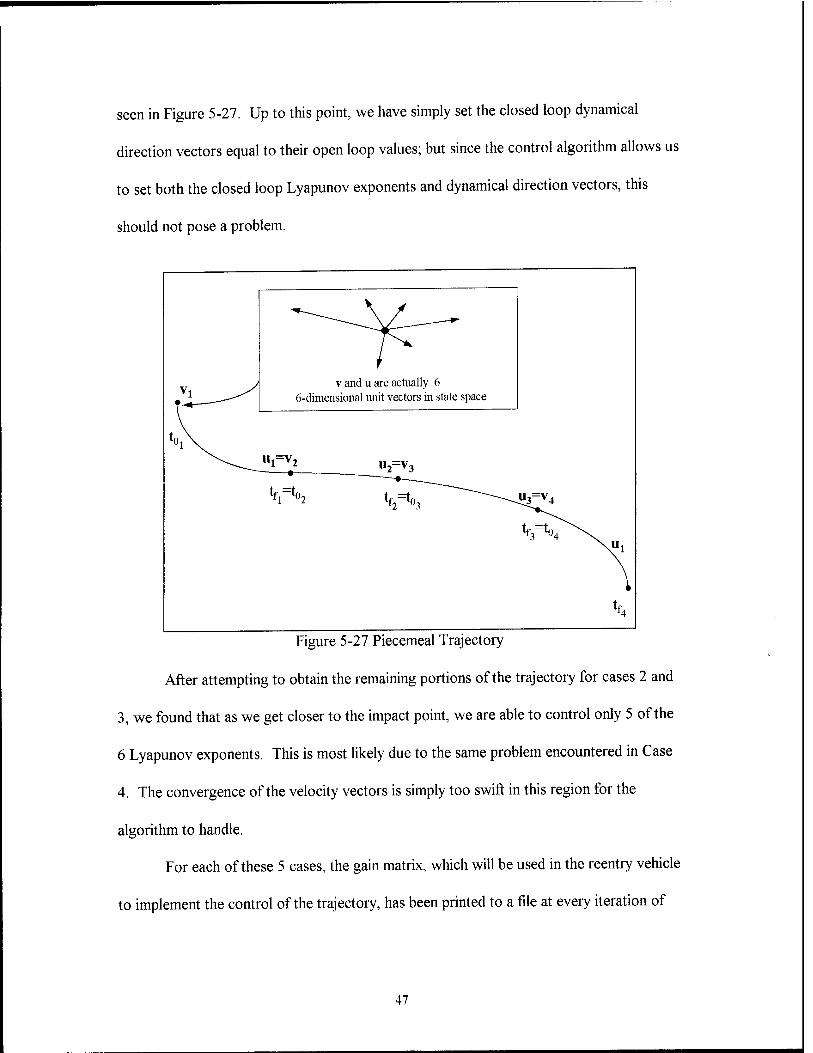
seen in Figure 5-27. Up to this point, we have simply set the closed loop dynamical

direction vectors equal to their open loop values; but since the control algorithm allows us

to set both the closed loop Lyapunov exponents and dynamical direction vectors, this

should not pose a problem.

v and u are actually 6 6-dimensional unit vectors in state space

=Vi

tf=to tf2=to3 »3^4

%=\

%

Figure 5-27 Piecemeal Trajectory

After attempting to obtain the remaining portions of the trajectory for cases 2 and

3, we found that as we get closer to the impact point, we are able to control only 5 of the

6 Lyapunov exponents. This is most likely due to the same problem encountered in Case

4. The convergence of the velocity vectors is simply too swift in this region for the

algorithm to handle.

For each of these 5 cases, the gain matrix, which will be used in the reentry vehicle

to implement the control of the trajectory, has been printed to a file at every iteration of

47

For each of these 5 cases, the gain matrix, which will be used in the reentry vehicle

to implement the control of the trajectory, has been printed to a file at every iteration of

the trajectory, along with the time and the state vector at that time. To ensure that these

gains can be implemented in the real world vehicle, we will graph the individual

components of the gain matrix vs time. A plot of this type for Case 1 can be seen in

Figure 5-28.

50 250 300 100 150 200 time

Figure 5-28 Case 1: Gain Plot

There seem to be several points which require very high gain to stabilize them. We

can see from Figure 5-4 that these seem to occur at the point in the trajectory where the

vehicle is going through a sizable deceleration due to aerodynamic forces. It would make

sense that at this point the vehicle would be hard to control. It appears as though these

48

problem points may go to a gain value of infinity which would signify that although the

control algorithm was able to set the Lyapunov exponents, it required an unrealistic,

unachievable amount of control by the mechanical systems of the vehicle to accomplish it.

Therefore, while the algorithm is able to specify stable Lyapunov exponents, the real

world system would not be able to accomplish them.

Figures 5-29 through 5-32 show the gain plots for the other 4 cases. We see that

these are very similar to the plot for Case 1. Looking at acceleration vs time plots for

these cases, we can see that most of the problem points seem to appear in the area of

maximum deceleration in the trajectory. One possible method for eliminating these spikes

of infinite gain is to choose the stable Lyapunov exponents such that the control algorithm

is able to accomplish the required trajectory without resorting to infinite gain. Despite

numerous attempts, we were unable to choose Lyapunov exponents which allowed a finite

gain at all points. We were, however, able to change the position and number of infinite

spikes.

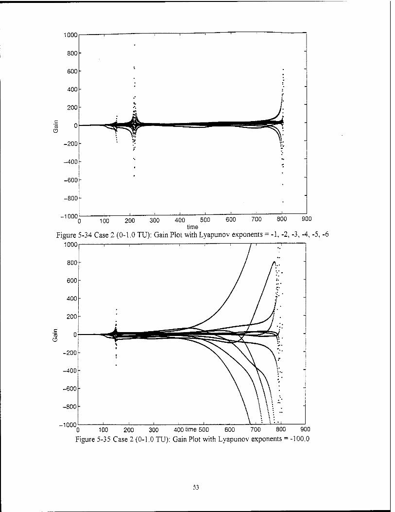
Figures 5-33 through 5-35 are gain plots of the shortened trajectory of Case 2 with

the desired closed loop Lyapunov exponents changed. Notice in Figure-33, where the

Lyapunov exponents were all set to zero, there are only three spikes, with one being at the

very end of the trajectory. All other times have very reasonable gains. Figure 5-34, which

had Lyapunov exponents of-1, -2, -3, -4, -5, and -6, has the same number of spikes, but

the two mid-trajectory spikes have moved much closer together. Figure 5-34, where the

Lyapunov exponents are all set to -100.0, has only two infinite spikes, but the gain values

towards the end of the trajectory get very large long before they actually go to infinity.

49

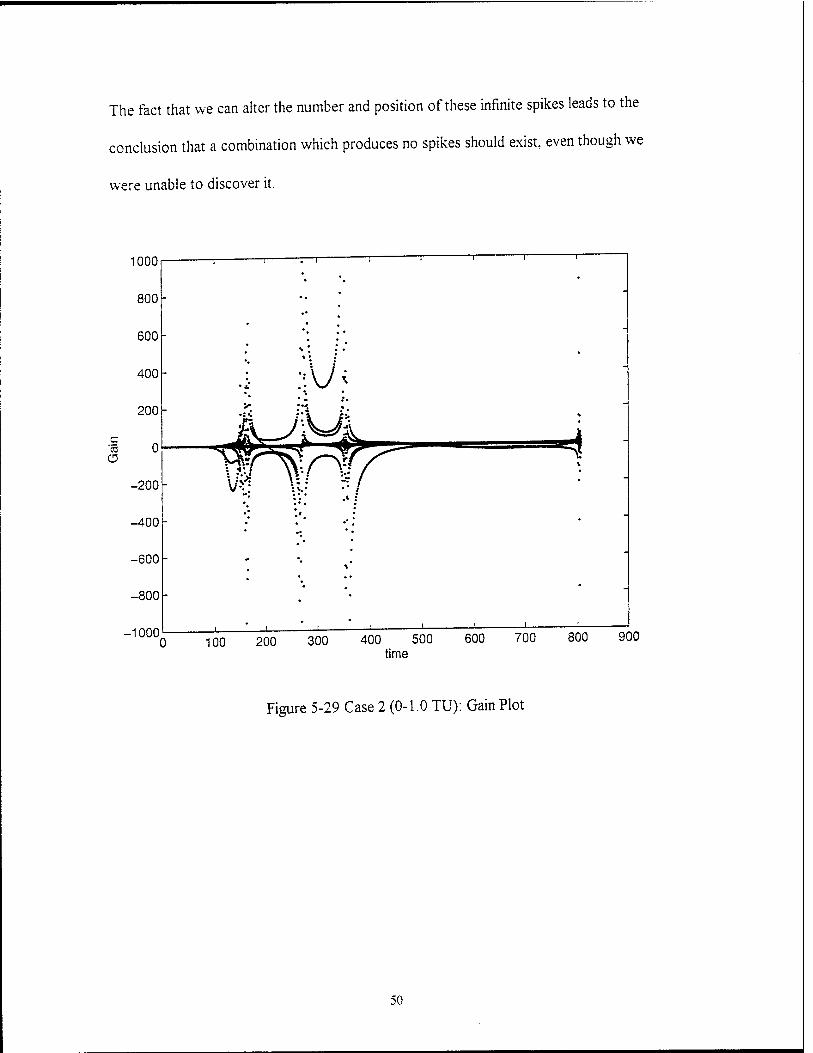
The fact that we can alter the number and position of these infinite spikes leads to the

conclusion that a combination which produces no spikes should exist, even though we

were unable to discover it.

400 500 600 700 800 900 time

Figure 5-29 Case 2 (0-1.0 TU): Gain Plot

50

a

100 200 300 400 500 600 700 800 900 time

Figure 5-30 Case 3 (0-1.0 TU): Gain Plot

50 100 time 150 Figure 5-31 Case 4 (0-0.25 TU): Gai

200 ii Plot

250

51

100

80

■■'■■■ ' »-■' | [ i . i I ,

60 -

40

20

c 'rä 0 ü

■ * * ■

• \

^■■^v ' SS^/^JyT^* f*o/

-20 V/^y /'";■;' '• -40

. * * •

-60 V

-80

•i OCH 1 ! 1 1*1 -100 ( 3 50 100 150 200 250 300

-i nrtn

time „ . n. Figure 5-32 Case 5: Gain Plot

1UUU - - —; 1" ! i i i i i

800 -

600

400 / •

200

"5 0 o T*J^ ^ * # ^r — ^ -200

-400 .

-600

-800

-1000'- 0

.1 i i i i .

100 200 300 400 time 500 600 700 800 900

] Figure 5-33 Case 2 (0-1.0 TU): Gain Plot with Lyapunov exponents = 0.0

52

100 200 300 400 500 600 700 800 900 time

Figure 5-34 Case 2 (0-1.0 TU): Gain Plot with Lyapunov exponents = -1, -2, -3, -4, -5, -6 1000r

c "ca

0 100 200 300 400 time 500 600 700 800 900 Figure 5-35 Case 2 (0-1.0 TU): Gain Plot with Lyapunov exponents = -100.0

53

VI. Conclusions and Recommendations

6.1 Conclusions. Having looked at five cases and the control algorithm's ability to

control them, there are several conclusions we can draw. First, we must realize that these

test cases do not necessarily correspond to any operationally useful trajectories that a

Delta Clipper-like vehicle would fly. They were chosen because they had characteristics

which would challenge the bounds at which the algorithm performs. The initial control

law modeled in the vehicle was chosen to keep the vehicle at high altitudes for as long as

possible given the initial conditions. This may or may not be the desired objective of a

given reentry. Therefore, while only two of the cases were controlled in their entirety, we

can still claim to have successfully proven the strengths and weaknesses of Wiesel's

algorithm.

Cases 1 and 5 were handled completely successfully by the algorithm. Cases 2

through 4 are longer trajectories which have swift convergence of the velocity vectors in

the middle of the trajectory as the aerodynamic forces strongly affect the vehicle. While

this is a shortfall in algorithm performance, the inability of the algorithm to specify all

stable Lyapunov exponents in these cases is more based on the inherent characteristics of

the trajectories themselves than the robustness of the control algorithm. From the results

of the previous section it is clear that the algorithm can handle pole placement for large

arcs, if not entire trajectories for most reentry situations. Another problem became

apparent when comparing the desired and achieved closed loop dynamical direction

54

vectors. Certain vectors ended up being the negative of their desired values. While no

information is lost, this is still something that needs to be addressed.

Another weakness was discovered in the gain matrices produced by the program.

For randomly chosen stable exponents, the gain matrix produced by the algorithm had

several points which approached infinity. This is obviously a problem since no real world

system would be able to implement such gain. While changing the desired Lyapunov

exponents affected the number and location of these infinite spikes, we were unable to

totally eliminate them. The ability to affect the singularities by changing the desired

Lyapunov exponents leads to the conclusion that choosing the correct exponents would

allow the gain matrix to be finite.

Still, despite the weaknesses stated above, the usefulness of this algorithm should

not be overlooked. The ability to place the poles and dynamical direction vectors of a

given chaotic time dependent system without modeling it as a constant coefficient system

is invaluable. Due to the nature of chaotic systems, there may be some limits on the length

of time a given system can be controlled. This will tend to be a problem for any control

algorithm dealing with time dependent chaotic systems. Wiesel's method gives us the

ability to do realistic control for long periods of time.

6.2 Recommendations There are several areas which rate further research before

Wiesel's control algorithm can be termed a complete success. The research in this paper

concentrated on a Delta-Clipper like vehicle with two control variables and a given control

law. A more vigorous test of the algorithm would be to vary the vehicle's control law for

55

given initial conditions and evaluate how the algorithm handles the different trajectories.

Another possible test would be to increase the number of control variables and vary the

control matrix away from the identity matrix which was used in this research.

More work should be done in determining the exact reasons for and quantifying

the boundaries of the inability of the algorithm to handle long arcs of trajectory. While we

discussed the dual sweep algorithm and the difficulties it poses, the actual limits of the

Linear Quadratic Regulator as well as possible alternative methods need to be explored in

depth.

As stated earlier, the problem with the SVDCMP subroutine, which returned the

negative of the u and v vectors in a seemingly random pattern, needs to be evaluated

further. This is a situation which can be worked around in the short term since the

resulting values are simply the negative of the desired vectors. This may well be a

problem which can be solved by implementing a different decomposition routine, but the

matter needs to be examined.

Finally, the problems with the gain matrix discussed above need to be more

thoroughly examined. Other possible methods for calculating the gain matrix need to be

evaluated as do the ranges of acceptable stable exponents. More work needs to be done

to see if it is possible to choose stable exponents that actually give finite gain at all points.

If we are eventually able to iterate through exponents and pick ones which do not cause

infinite spikes, we should be able to discover an algorithm which takes this into account

when calculating the gain matrix. At the very least, there should be a method of

determining, at the outset of the problem, which Lyapunov exponents would tend to move

us closer to a continuously finite gain matrix vs those that would move us away from one.

56

While, overall, Wiesel's algorithm is both very powerful and very useful, addressing these

issues could lead to a more full proof method which has the potential to gain acceptance

throughout the control community.

57

Bibliography

1. Bate, Roger R., Donald D. Mueller, and Jerry E. White, Fundamentals of Astrodvnamics. New York, Dover Publications Inc. 1971.

2. Breakwell, J.V., A. Kamel, and M.J. Ratner, "Stationkeping for a Translunar Communications Station," Celestial Mechanics, Vol. 10, 1974, pp357-373

3. Bryson, Arthur E., Jr and Yu-Chi Ho, Applied Optimal Control: Optimization, Estimation and Control. New York, John Wiley and Sons, 1975 pp 148-152

4. Copper, John A. "Future Single-Stage Rockets: Reusable and Reliable" Aerospace America. February 1994. pp 18-21

5. Copper, John A. "Single Stage Rocket Concept Selection and Design" AIAA Space Programs and Technologies Conference. March 24-27, 1992 Paper 92-1383

6. Eshbach, Ovid W. and Mott Souders, ed. Handbook of Engineering Fundamentals. New York, John Wiley & Sons, 1975.

7 EtterD.M. Structured FORTRAN 77 for Engineers and Scientists. Reading, Massachusetts, Benjamin/Cummings Publishing Company Inc. 1983.

8. Gaubatz, William A. and Jess Sponable. "A Technology and Operations Assessment of Single Stage Rocket Technology Flight Test Program Results." AIAA 1993

9. Ladner, Pat and Jess Sponable. "Single-Stage-Rocket-Technology: Program Status and Opportunities. "AIAA 1992

10. Regan, Frank J. and Satya M. Anandakrishnan. Dynamics of Atmospheric Reentry. Washington DC: American Institute of Aeronautics and Astronautics, Inc., 1993.

11. Vinh, Nguyen X., Adolf Busemann and Robert D. Culp, Hypersonic and Planetary Entry Flight Mechanics. Ann Arbor, University of Michigan Press, 1975

12. Wiesel, William E. and Robert A. Calico. "Control of Time-Periodic Systems." Journal of Guidance Control and Dynamics. Vol 7, No. 6, Nov - Dec 1984 pp671-676.

13. Wiesel, William E. "Full Stability Exponent Placement in Chaotic Systems." Phys. Rev. E, 1995, Preprint

14 Wiesel, William E. "Optimal Pole Placement in Time-Dependent Linear Systems." Journal of Guidance Control and Dynamics. vl8, 1994, pp995-999.

58

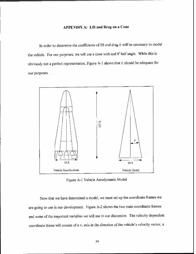
APPENDIX A: Lift and Drag on a Cone

In order to determine the coefficients of lift and drag it will be necessary to model

the vehicle. For our purposes, we will use a cone with and 8° half angle. While this is

obviously not a perfect representation, Figure A-l shows that it should be adequate for

our purposes.

r-

18ft

Vehicle Specifications

18ft

Vehicle Model

Figure A-l Vehicle Aerodynamic Model

Now that we have determined a model, we must set up the coordinate frames we

are going to use in our development. Figure A-2 shows the two main coordinate frames

and some of the important variables we will use in our discussion. The velocity dependent

coordinate frame will consist of a vi axis in the direction of the vehicle's velocity vector, a

59

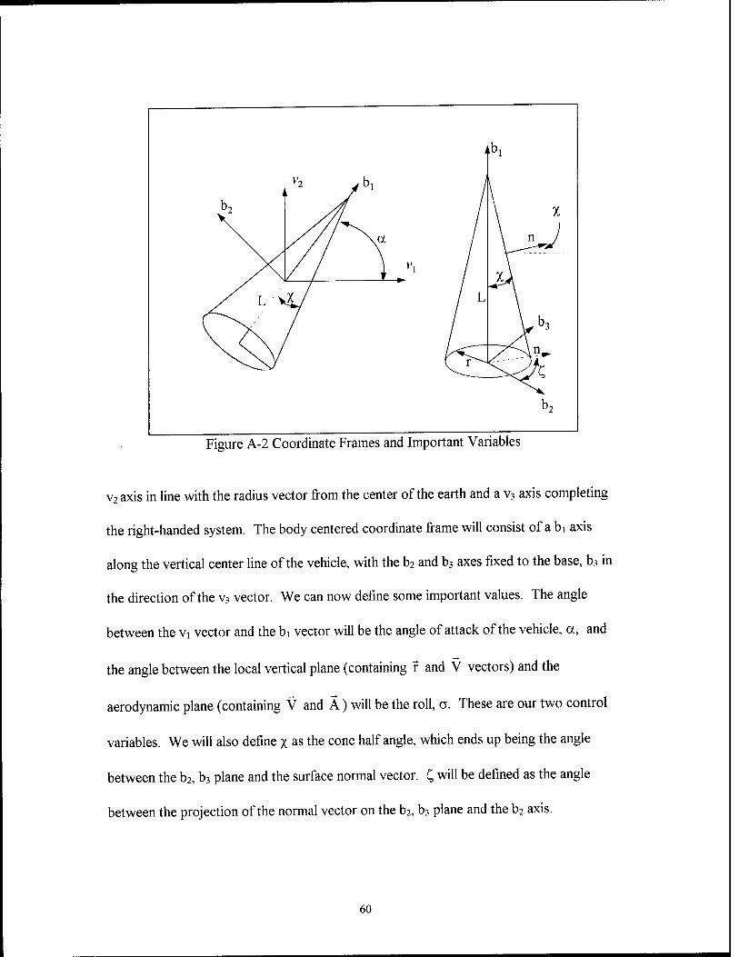
Figure A-2 Coordinate Frames and Important Variables

v2 axis in line with the radius vector from the center of the earth and a v3 axis completing

the right-handed system. The body centered coordinate frame will consist of a bi axis

along the vertical center line of the vehicle, with the b2 and b3 axes fixed to the base, b3 in

the direction of the v3 vector. We can now define some important values. The angle

between the vi vector and the bi vector will be the angle of attack of the vehicle, a, and

the angle between the local vertical plane (containing r and V vectors) and the

aerodynamic plane (containing V and A) will be the roll, o. These are our two control

variables. We will also define % as the cone half angle, which ends up being the angle

between the b2, b3 plane and the surface normal vector. C, will be defined as the angle

between the projection of the normal vector on the b2, b3 plane and the b2 axis.

60

With these definitions accomplished, we are now able to write the equation of the

normal vector from the surface of the cone as follows:

n = Sin(X)b, - Cos(x)Cos(Qb2 + Cos(x)Sin(Qb3.

Using the following coordinate transform,

b, = Cos(a)v, + Sin(a)v2

b2 = -Sin(a)v, + Cos(a)v2,

b3=v3

we are able to determine the normal vector in terms of the velocity coordinate frame.

n = (Sin(/)Cos(a) + Cos(x)Cos(C)Sin(a))v,

+ (Sin(x)Sin(a) - Cos(x)Cos(C)Cos(a))v2

+ (Cos(x)Sin(C))v3

Now if we look at an infinitesimally small surface element of the cone in Figure A-3, we

L Tan(x) /

i i

\^l ^Ltan(X)dC

\ Xxäx=dL/Cos(x)

^n Figure A-3 Surface Element

61

can carry the derivation farther and determine the incremental area, such that

LTan(x) dS

Cos(x) ■dLdC

Then, if we picture the surface element flying through the reentry trajectory, we can see

that the mass intercepted over time dt is as follows

dm = dSh»Vdtp.

Now that we have the mass and the velocity, we will be able to calculate the change in

momentum. Looking at Figure A-4, we can see the value of the change in momentum,

Ap.

dp. =dmv 'in

^\. /

"\ n / 4ji=-2dm(v»n)n

\ \^

«-V ^

Figure A-4 Change in Momentum

Knowing this and assuming that the altitude and speed of the vehicle allow us to model the

air as a Newtonian fluid, we are able to use Newton's third law to calculate the

aerodynamic force, Fd in the following manner:

dFd = ^ = -2(n. v)2pdSn = -2(n« v)2p^^dLdCn, dt Cos(x)

62

which leads to the following.

Fd =-2JdLjdC(Sin(x)Cos(a) + Cos(x)Cos(C)Sin(a)) v2p

xLTanOOxs

Cos(x)

(Sin(x)Cos(a) + Cos(x)Cos(C)Sin(a))v,

(Sin(x)Sin(a) + Cos(x)Cos(C)Cos(a))v2

(Cos(x)Sin(a))v3

In this equation, the vi component is the drag component, the v2 is the lift

component and the v3 component is the side force component. Based on Figure A-5, we

can see that the amount of surface area, while dependent on the angle of attack can not be

handled by a single integral. When the angle of attack gets larger than the cone half

Velocity

angle of attack

Velocity

Side Views

Nose On Views Figure A-5 Angle of Attack vs Surface Area

angle, the nose is now outside the original circular cross section. If we consider the

extreme where the normal vector to the surface and the velocity are perpendicular, we can

63

perform the following development.

n« v = 0

Sin(x)Cos(a) + Cos(x)Cos(QSin(a) = 0

Cos(x)Cos(C)Sin(a) = -Sin(x)Cos(a)

Cos(C) = -|!^^=Ta„(x)C,n(«) Cos(x)Sin(a)

This means that when the angle of attack is less than the half angle of the cone,

Cos(C) < -1 and therefore the limits of C are±7i. If a > x then Cos(Q > -1 and

therefore C = Cos^1 (-Tan(x)Ctn(a)). From the text, we know the definition of Lift and

Drag, so referring back to Figure A-2 and the fact that the area of the base of the triangle

is A = 7ir2 = 7iL2 Tan2(x), results in the following equation.

CDL2 _ CD

A2 ltTan2(x)

By rearranging the equations of lift and drag and substituting them into the

previous equation, we get the following equations which can be used to determine the

64

coefficients of lift and drag based on the angle of attack.

c, 3A = = L2 xj.

c, A = Fd#V2

}/pv2 = L2 4

2(Sin(x)Cos(a) + Cos(x)Cos(QSin(a)) 2 Tan(x)

Cos(x) ((Sin(x)Cos(a) + Cos(x)Cos(QSin(a)

dC

2(Sin(x)Cos(a) + Cos(x)Cos(C)Sin(a))

x(Sin(x)Cos(a) + Cos(x)Cos(C)Cos(a)

2 Tan(x) Cos(x) dC

where c± = - ± 7C when a < x ]

±Cos"'(-Tan(x)Ctn(a)) when a>xj

The graph of angle of attack vs CD and CL, resulting from these can be seen in the text in

Figure 2-2.

65

APPENDIX B: Equation of Variation

When we integrate the state vector through a given trajectory, we are concerned

with more then just one ideal trajectory. We would like to be able to determine the

characteristics of nearby trajectories. We define the phi matrix, $, as the n-dimensional

matrix of small differences between some reference trajectory and a given trajectory very

near it. The use of a phi matrix allows us to specify how initial errors in the trajectory

propagate through to final errors. In order to obtain a final phi, we must have an equation

of motion to propagate the phi matrix. In order to generate this equation, we will start

with a reference or ideal trajectory and another trajectory which starts from a point whose

initial conditions are the original I.C.'s plus a small 5x as seen in Figure B-l.

reference trajectory

nearby trajectory

Figure B-l Reference Trajectory

Now if we take the equation of the nearby trajectory to be x = xr (t) + 8x(t), we

66

get the following equation of motion for the nearby trajectory,

x = xr(t) + 8x(t) = f((xr+8x),t).

Taking the Taylor series yields

xsf(xr,t)+ — Sx + H.O.T.. dx „

■V

We know that xr (t) = f(xr ,t). Using this and truncating the higher order terms gives us

the equation of variation as follows:

- of ^ Sx = — 8x

dx.

pif -* By the definition A = — and this equation we get the equation of variation, 8x = ASx .

dx

From the definition of the phi matrix, we know that it is simply the square matrix of the

Sx's. So we now have the following equation of variation:

Ö = A(t)0>

By convention, the phi matrix at time equals zero, ®(t0, t0), is equal to the identity

matrix, I. So we are now able to extend our knowledge of the reference trajectory to all

the nearby trajectories by simply calculating the A matrix and using it in the equation of

variation.

67

APPENDIX C: A Matrix Equations

dt — = 0 dr

*=0 dd

aj)

5f

3v Siny

— = vCosy

öij) _ vCosySinv|/

cd

cty

0

= 0

ö<j> _ CosySin\|/

dv r

3(j) _ -vSinySin\|/

dy r

<3cj> _ vCosyCosy

d\\) r

Equations

vCosyCosv|/Sec9

3r ~~ r2

c©_ 0 ae~

dd _ vCosyCosv|/Sec(j)Tan(t)

dfy~ r

dQ _ CosyCos\|/Sec())

dv' r

dQ -vCosv(/SinySec())

dy = r

dd -vCosySinvj/Sec(|)

d\\> r

dv = 0 ¥"

dv _ = 0

cQ~

dv = 0

äfr~ dv _ CdPSv

dv m

dv = -gCosy

öT dv — = 0 d\\i

dy vCosy SCLV2COSG

ck r2 2m

59

aj>

fCLpSvCoso | 2vCosy'N

dy _

Sv

V m T J

V

dy _

dy

f A g— Siny

CLpSvCosa

2m

-> v"

\

g— Cosy r J

= 0

d\\i vCos\j/CosyTan(j)

dr ■f

V

d\\i = 0

d\\r vCos\|/CosySec2(|)

cty ~ r

chj/ _ CLpSSecySina _ Cos\|/CosyTati(|)

cV ~ 2m r

dvj/ _ vCosvj/SinyTatK)) vCLpSTanySecySina

dy r 2m

dvj/ _ vCosySin\i/Tan(()

d\\i r

69

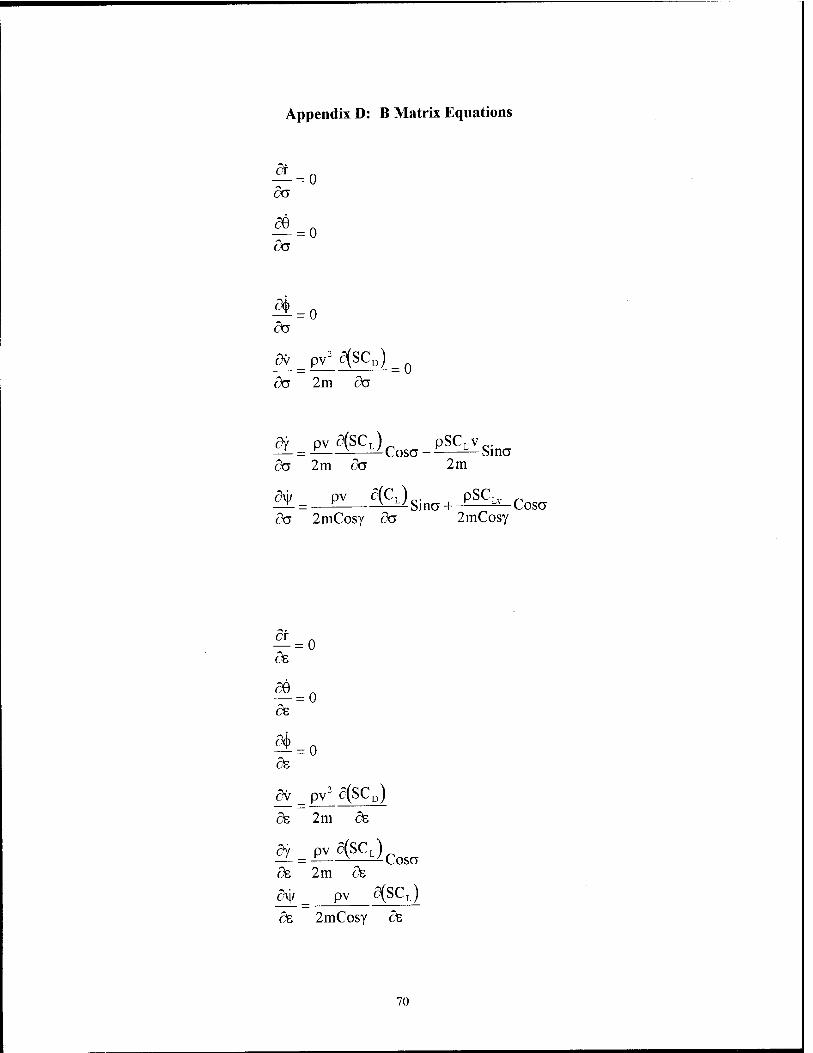
Appendix D: B Matrix Equations

da

da

*=0 da

av_Pv2g(scD)_o

da 2m da

iUf»3&lc«o-H^Sin<, 5a 2m 5o 2m

^= pV a(C^Sina + -P^^Cosa da 2mCosy da 2mCosy

de' 0

59 _ 5e "

= 0

aj>_ 5e~

= 0

5v pv2 5(SCD)

5e 2m de

5y_

5s =

PV^

SCL)COSO

2m 5e

5\j/ pv 5(SCL)

5e 2mCosy 5e

70

APPENDIX E: Flowchart for Program DESIGN

Reset CL value & set flag

Yes

Start

Accept Input File

X Determine max

CD and CL

X Initialize phi matrix

Set inital roll and angle of attack

EC

Initialize HAMING

HE

Integrate Trajectory

Determine & print impact time

f Stop J

Is radius \ No less than the radius

of the Earth?

Print important states to output files

71

APPENDIX F: Flowchart for Program FIRST

Start

Accept Input File

I Initialize phi matrix

X

Initialize HAMING

Calculate open loop Lyapunov exponents and principal

directions I

Output two copies of Lyapunov exponents and principal directions to file

(<T)

72

APPENDIX G: Flowchart for Program BVP

( Start J ±

Accept Input File / Is radius \^

^-►@ 1 Construct Desired

phi matrix

/less than the radius. >v of the Earth?/

1 Initialize phi & phi Lagangian matrix lYes

1 Determine phi perturbed Initialize HAMING

| h^

\ Calculate phi

Lagrangian partials Integrate Trajectory i

1 Get phi

Lagrangian at t=t0

/ Is radius \^ -^0

/less than the radius/ ►"

|

Calculate S0 matrix

\ of the Earth?/ 1 Initialize states, phi.

& phi Lagrangian

lYes |

Initialize HAMING Construct & print error vector 1

| Integrate Trajectory L 1^

Set delta value

| 1^ Print Gain matrix,

time and state i

vNo ^

\ Set up Loop 1:

1 to order |

Set up Loop 2: 1 to order

| / Is radius \

Initialize states, phi, & phi Lagrangian

/less than the radius, \of the Earth?/

1 Perturb Loopl,Loop2

element of phi Lagrangianby delta

|Yes

Determine & print final phi 1 '

Initialize HAMING 1 Calculate Lyapunov

exponents and principal directions

|-^ © Integrate Trajectory

t ( End J i

73

AERO

TYPE:

PURPOSE:

INPUTS:

OUTPUTS:

CALLS:

AUTHOR:

Appendix H: Code Summary

Subroutine

This routine iterates through a list of data points to determine the CD and CL values for a given angle of attack. Once the closest data point is found, the code uses interpolation to get the exact values of CD and CL. The numerical derivatives of CD and CLwith respect to angle of attack are also calculated.

Angle of Attack

Coefficients of Drag and Lift Partials of the coefficients of Drag and Lift with respect to Angle of Attack

None

William E. Wiesel

ATM

TYPE:

PURPOSE:

Subroutine

This routine determines the temperature, density and pressure at the current altitude of the vehicle.

INPUTS: Altitude, Density at sea level

OUTPUTS: Pressure, Temperature, and Density at altitude.

CALLS: None

AUTHOR: Michael H. Platt

74

BVP

TYPE:

PURPOSE:

INPUTS:

OUTPUTS:

CALLS:

AUTHOR:

Main Program

This program solves the boundary value problem such that the numerical partials of the phi matrix are determined and used to determine what gain will be needed to achieve the final Lyapunov exponents and principal direction vectors.

State initial Conditions Control history of flight Open loop Lyapunov exponents and principal direction vectors. U and V Desired closed loop Lyapunov exponents and principal vectors U and V

Gain as a function of time Achieved phi matrix Achieved Lyapunov exponents and principal direction vectors, U and V

HAMING LEQT2F LINV1F SVDCMP

Dr William E. Wiesel modified bv Michael H. Platt

DESIGN

TYPE:

PURPOSE:

INPUTS:

OUTPUTS:

CALLS:

AUTHOR:

Main Program

The purpose of this program is to design the reentry trajectory of the vehicle based on the initial conditions provided. This code makes use of a control law which is specified in the text of this paper.

Initial state conditions Parameter values initial control variables

Control history of trajectory Miscellaneous plot files Final state and control values

AERO HAMING

Dr William E. Wiesel modified bv Michael H. Platt

75

DYNAM

TYPE:

PURPOSE:

Subroutine

This subroutine implements the control law which keeps the vehicle at maximum altitude for as long as possible. It also calls the various subroutines to determine CD, CL, and characteristics of the atmosphere at altitude.

INPUTS: nxt (flag)

OUTPUTS. Equations of Motion A matrix B matrix

CALLS: AERO ATM

AUTHOR: Dr William E. Wiesel modified by Michael H. Platt

FIRST

TYPE:

PURPOSE:

INPUTS:

OUTPUTS:

CALLS:

AUTHOR:

Main Program

This program iterates through the trajectory, takes the phi matrix, decomposes it and calculates the open loop Lyapunov exponents and the principal direction vectors, U and V. It then outputs these to a file which will eventually be used in the program BVP.

Initial Conditions Parameters Control History of Trajectory

Open Loop Lyapunov exponents Open Loop Principal Direction Vectors

HAMING SVDCMP

Dr William E. Wiesel modified by Michael H. Platt

76

HAMING

TYPE:

PURPOSE:

INPUTS:

Subroutine

This routine is an ordinary differential equations integrator. It uses a fourth order predictor-corrector algorithm such that it carries along the last four values of the state vector. It extrapolates these values to obtain the next value (the prediction part) and then corrects the extrapolated value to find a new value for the state vector.

state vector

OUTPUTS:

CALLS:

AUTHOR:

State vector

RHS

Dr William E. Wiesel

LEOTF

TYPE:

PURPOSE:

Subroutine

This routine is a linear equation solver, which makes use of Gaussian elimination with maximal pivoting.

INPUTS:

OUTPUTS

CALLS: None

AUTHOR: IMSL

Matrices A and B from the equation Ax=B

x from the above equation

77

LINV1F

TYPE: Subroutine

PURPOSE: This subroutine inverts a matrix

INPUTS: Matrix to be inverted

OUTPUTS: Inverted matrix

CALLS: None

AUTHOR: IMSL

RHS

TYPE: Subroutine

PURPOSE: This routine calculates the quantity the phi matrix.

INPUTS: state vector

OUTPUTS: Equations of Motion A phi

CALLS: DYNAM

AUTHOR: Dr William E. Wiesel modified bv Michael H. Platt

SVDCMP

TYPE: Subroutine

PURPOSE: This routine performs the singular value decomposition of the input matrix.

INPUTS: Matrix top be decomposed

OUTPUTS: Resulting vectors and diagonal matrix

CALLS: None

AUTHOR: "Numerical Recipes" [pp60-64]

78

APPENDIX I: Input Files

DESIGN.IN

# of States, # of Parameters, # of Controls Parameters Initial State Conditions (radius, longitude, latitude, velocity, flight path angle, heading) Initial Control Conditions (roll, pitch) Maximum Time, # of Points, # of Points to Skip

FIRST.IN

# of States, # of Parameters, # of Controls Parameters Initial State Conditions (radius, longitude, latitude, velocity, flight path angle, heading) Initial Control Conditions (roll, pitch) Maximum Time, # of Points, # of Points to Skip

BVP.IN

# of States, # of Parameters, # of Controls Parameters Initial State Conditions (radius, longitude, latitude, velocity, flight path angle, heading) Initial Control Conditions (roll, pitch) Maximum Time, # of Points, # of Points to Skip Open Loop Lyapunov Exponents Open Loop Principal Direction Vectors U and V Desired Closed Loop Lyapunov Exponents Desired Closed Loop Principal Direction Vectors U and V Order of Control Matrix Control Matrix

79

APPENDIX J: Open Loop Dynamical Direction Vectors

CASE1 u

1 1 -0.01028543050235800060

2 1 0.00363444199734480004

3 1 -0.00000000000000469740

4 1 0.08214474583247899364

5 1 0.99656070637109994692 6 1 -0.00000000001125988246

-0.97168401832455997269

0.00003107162937948000

0.00000000000002290337

-0.03569012010809000102

-0.23357307827285000990

-0.00000000000009349885

1 2 -0.00089665641974298995

2 2 -0.99996954401282001079

3 2 -0.00000000000011928163

4 2 0.00712768995717460042

5 2 0.00305009670780599998

6 2 -0.00000000001996683656

0.00796246377915789914

-0.97579409007383999253

0.00000000000453068203

-0.21854627299113998928

0.00013967542602473000

-0.00000000001895038530

1 3 -0.12171244904868999681

2 3 0.00690662913636379966

3 3 0.00000000000000457848

4 3 0.98908086295801000976

5 3 -0.08280956919816499784

6 3 0.00000000000058194711

0.22179652742774000340 0.10524131864098999756

-0.00000000000204756123

-0.46235891461048000961

-0.85202981130470001325

0.00000000000862846213

1 4 -0.99251170555979995047

2 4 0.00001876508221094700

3 4 -0.00000000000000005374

4 4 -0.12214943020019999875

5 4 -0.00017514685499890999

6 4 -0.00000000000000003907

-0.08107446036942800305

0.19170330634143001314

0.00000000000001332149

-0.85859651523201996337

0.46849631614879999608

-0.00000000000008494051

1 5 -0.00000000000006291855

2 5 -0.00000000001992965083

3 5 0.00771671613673619982

4 5 0.00000000000049162056

5 5 0.00000000001132995245 6 5 0.99997022570278004672

-0.00000000000191225029

-0.00000000001992963855

-0.23082828392586998700

-0.00000000000023507429

0.00000000000757627134 0.97299450324236003151

1 6 0.00000000000000096663

2 6 0.00000000000003463015

3 6 0.99997022570278004672

4 6 -0.00000000000000700461

5 6 -0.00000000000008201465

6 6 -0.00771671613673600033

0.00000000000000000000 0.00000000000003458703

0.97299450324236003151

0.00000000000000149329

0.00000000000000278481

0.23082828392586998700

80

CASE 2 (0.0-1.0 TU) u

1 1 -0.06513334848611600225 2 1 0.08123799463349500039 3 1 -0.09214490890452099736 4 1 0.40856082818428002268 5 1 -0.53349110099935004303 6 1 -0.72741504365373998997

-0.98233526721117003788 0.00001966208784733900 0.00012344799140762001

-0.03676190204151300045 -0.18348284244442000790 -0.00012749098910065000

1 2 -0.05909772630751399664 2 2 -0.42440813732748000620 3 2 0.34883167171661999539 4 2 -0.29514532828202000303 5 2 -0.72701775086806996740 6 2 0.28113356547897999649

0.10507018593484999947 -0.08834185895499800656 -0.00026492752091081002 -0.90984883644657998936 -0.38030822618972998095 0.09325582934395500179

1 3 -0.99488239960038005183 2 3 0.00000217186183196260 3 3 0.00002335921155600400 4 3 -0.03458991987095100251 5 3 0.09493443608945199841 6 3 0.00002650879976210500

-0.12758862379124999431 0.03746385565551300229 -0.10489380108456000662 -0.26425770193451997292 0.73554924314832004217 0.60037494198603003071

1 4 0.00659393826681990008 2 4 -0.61186947499749000379 3 4 -0.77535346913045000150 4 4 -0.14171256413912999839 5 4 0.01769099672166399989 6 4 -0.06327591367903200037

-0.06457644432611399365 -0.56030766996837999550 -0.39874751101654998253 -0.17243074346014000686 0.38036046915558002768 -0.59032124515761996708

1 5 -0.02818112547849700028 2 5 -0.29353527557349001764 3 5 0.04090872648305499820 4 5 0.85124937207759998614 5 5 0.01470462107028499936 6 5 0.43188843804269999582

0.05840774375848799965 -0.49957398211156001100 -0.53008406985981004755 0.26096667465457001889 -0.36575846116713001122 0.51394785100386997101

1 6 0.04045319234070700321 2 6 -0.59391153276705999087 3 6 0.51670035226388999483 4 6 -0.00792956572542049924 5 6 0.42105901091864000874 6 6 -0.44866447124517999656

-0.01082775170848999935 -0.65366147695959997410 0.74095108233067996650 0.05617435155750000186 0.04704967707934799848 0.13502480156904000941

CASE 3 (0.0 -1.0 TU) u

1 1 -0.06389959006247300510 2 1 0.07831410885031099556 3 1 -0.07481340127633999415 4 1 0.36301192648443997291 5 1 -0.56829488266759997650 6 1 -0.72763312548164005289

-0.98258845740532996249 0.00001413839874403200 0.00009350141821937500

-0.03477221682566800087 -0.18251246080158001206 -0.00009497680907610600

1 2 -0.05264048512495699689 2 2 -0.46576529173300001974 3 2 0.31555588699281000853 4 2 -0.30706995163021000295 5 2 -0.69832947170930004255 6 2 0.31426127390260000238

0.10385091218924000223 -0.10843137532169999648 -0.01516064742741900055 -0.90317797911088004703 -0.38709910220319998508 0.10794259018358999536

1 3 0.00508511554381889993 2 3 -0.52968321718317001867 3 3 -0.83826363559234995382 4 3 -0.12253006393467000268 5 3 0.00992349524661539917 6 3 -0.04014742771513900299

-0.06392369442280200487 -0.48472424352228998812 -0.48575829257165997754 -0.17365098034786000114 0.37725113305793001039 -0.59373560602483999027

1 4 0.99534969609505996591 2 4 -0.00000171062338637060 3 4 -0.00001901692147163200 4 4 0.03415835918811700039 5 4 -0.09006768631214200072 6 4 -0.00002233515044160400

0.12658611719581999711 -0.03617232547061600273 0.10619068515049999435 0.25712774058570997404 -0.73011780701259998416 -0.61008554244057000560

1 5 -0.03071106195926399940 2 5 -0.26391747948327998197 3 5 0.01941350196523499924 4 5 0.87042914625278000607 5 5 -0.00938157158515089996 6 5 0.41387509964507002147

0.05812527505084000290 -0.45890691292737001428 -0.55742526528196001401 0.28956397897627000892 -0.36867962124332998020 0.50550075198002997201

1 6 0.03815463893647400018 2 6 -0.65323261310700997395 3 6 0.43790938560041997585 4 6 0.01015270009756000062 5 6 0.42553283952603998541 6 6 -0.44596577432547002129

-0.01568693839398100157 -0.73578601000916998842 0.66468762530795999499 0.05425675175635699676 0.07435317138578399765 0.08995020286136899690

82

CASE 4 (0.0 -0.25 TU)

1 1 -0.00424501835640509959 2 1 0.00486853551608860003 3 1 0.00051177705371614995 4 1 -0.00365524018172130004 5 1 -0.98150231201513005175 6 1 -0.19130568730045999226

-0.98275212517203003326 0.00002020102189509900 0.00014408704217409000 -0.01788005846675300159 -0.18405959217574999198 -0.00078060107066167997

1 2 0.00015856428007883001 2 2 -0.98598227258126003303 3 2 -0.03237860992992400155 4 2 0.00068161489029038003 5 2 0.02656846007968500026 6 2 -0.16150607097566999082

0.02342717615886300009 -0.96373444626989002160 -0.00289809927635030018 -0.18260604405283001328 -0.10677154859475999904 -0.16097687596897999884

1 3 0.00081477086986990997 2 3 0.16243344365060999324 3 3 0.03600438154295500237 4 3 0.00096219023103698005 5 3 0.18943181631452998825 6 3 -0.96769471332630996319

0.01779211106295799927 0.164602243 94226000144 0.21131587728035000628 0.02973016257455799935 -0.09363821513029199628 -0.95827091377273998507

1 4 0.00002274309356453900 2 4 0.03781992876969399869 3 4 -0.99882683543490002887 4 4 0.00004280878599849200 5 4 0.00546410109994549965 6 4 -0.02974469788537199844

0.00168081358645540005 0.03781834147168299659 -0.97735343387202000542 0.00489308065307680028 -0.00932881973904150022 -0.20793326837375000760

1 5 -0.03369417688200600225 2 5 -0.00053312347196117005 3 5 -0.00003206112777283000 4 5 -0.99942425398929002345 5 5 0.00393192329604650018 6 5 -0.00034309305819740999

-0.17241850223978999468 -0.15944814598802001249 0.00892191453331350054 0.39359067675171000023 0.88278711677471999320 -0.10267343326363999323

1 6 -0.99942282981326002744 2 6 -0.00002585417719523500 3 6 0.00000039281516633206 4 6 0.03371064395236499783 5 6 0.00419511431231320026 6 6 0.00000892650091013410

0.06001586142085699876 -0.13140806574665001016 -0.00615182967721980035 0.90028544948462996267 -0.40810987146214000587 0.04499570965845500065

83

CASE 5

1 1 -0.01041367828494699915 2 1 0.00337819864074320004 3 1 0.00000000000001214309 4 1 0.08037935879455899990 5 1 0.99670421979557000114 6 1 -0.00000000000877931300

-0.97167057239938003921 0.00002933637589193600 0.00000000000001827429 -0.03571246813911099771 -0.23362559254466999659 -0.00000000000007401808

1 2 -0.00088850219598885004 2 2 -0.99997201756267994899 3 2 -0.00000000000015860298 4 2 0.00686937597676139967 5 2 0.00282600940400740000 6 2 -0.00000000001535902870

0.00792159671889250058 -0.97580439758499004643 0.00000000000341644084 -0.21850152435160000164 0.00033138383146531000 -0.00000000001457042648

1 3 -0.12504998895203001119 2 3 0.00667469197903149992 3 3 0.00000000000000257644 4 3 0.98881004102974001668 5 3 -0.08107189099091000051 6 3 0.00000000000035182400

0.22178708445351999479 0.10521059958065999418 -0.00000000000127910980 -0.46311014966396002457 -0.85162797522375000003 0.00000000000539344279

1 4 -0.99209539164917004417 2 4 0.00001877611933808500 3 4 0.00000000000000014074 4 4 -0.12548574864192998946 5 4 -0.00024577166175789001 6 4 0.00000000000000001726

-0.08126522139322900351 0.19166769818894999200 -0.00000000000016630747 -0.85820201162293996422 0.46920013268241000937 0.00000000000074047692

1 5 -0.00000000000006105413 2 5 -0.00000000001533198355 3 5 0.00627845312630180043 4 5 0.00000000000046327297 5 5 0.00000000000882206040 6 5 0.99998029031892998741

-0.00000000000112323390 -0.00000000001533197506 -0.23224721542661000417 -0.00000000000005440161 0.00000000000435169797 0.97265678989383996811

1 6 0.00000000000000088139 2 6 -0.00000000000006234910 3 6 0.99998029031892998741 4 6 -0.00000000000000529162 5 6 -0.00000000000006683849 6 6 -0.00627845312630120021

0.00000000000000000000 -0.00000000000006240077 0.97265678989383996811 -0.00000000000000078611 0.00000000000000261258 0.23224721542661000417

84

APPENDIX K: Closed Loop Dynamical Direction Vectors

Casel (Full Trajectory)

1 1 -0.01030196743589699947 2 1 0.00363519794936909999 3 1 -0.00000269712930276840 4 1 0.08215147129278900506 5 1 0.99655997723858003035 6 1 -0.00004823075400571100

-0.97168348266467996499 0.00003598647879645000 0.00000695859965293510 -0.03570886302410700153 -0.23357243750167999696 -0.00004140344651853700

1 2 -0.00089705510246072004 2 2 -0.99996953333970994837 3 2 -0.00000007726882264421 4 2 0.00712887931237249969 5 2 0.00305069197477219993 6 2 -0.00000653618027104730

0.00796202149669830023 -0.97579391837360995865 0.00000132604342975910 -0.21854705630080001333 0.00013865925542491000 -0.00000573366677570370

1 3 -0.12170074252679000115 2 3 0.00690777256897090030 3 3 0.00000126580746497530 4 3 0.98908156631773003209 5 3 -0.08281826900950700621 6 3 0.00003786428065245200

0.22180600744673001357 0.10524011426266000058 -0.00000708564145476850 -0.46234794239902998747 -0.85203344554194004878 0.00003460671460691000

1 4 0.99251295011246998268 2 4 -0.00001903828123642700 3 4 -0.00000134867301182800 4 4 0.12213914161319999740 5 4 0.00019164511472974000 6 4 -0.00019197112673628001

0.08105497925627799805 -0.19170483534745000331 0.00004290624056404200 0.85860142768133995705 -0.46849002173213999400 -0.00018033916462201999

1 5 0.00019464471915760001 2 5 -0.00000662625511493670 3 5 0.00766005984867070000 4 5 -0.00001000118430728300 5 5 0.00005127731661911400 6 5 0.99997064098065002735

-0.00003346437354563100 -0.00004499363566479400 -0.23088536749260998859 0.00017270391510402000 -0.00006654596705623000 0.97298094003864998847

1 6 -0.00000002622088171184 2 6 -0.00000002547469277593 3 6 0.99997066130583001087 4 6 -0.00000078855055026103 5 6 0.00000240046040188910 6 6 -0.00766006013041200043

-0.00000296158151728740 -0.00000012708358433498 0.97298095825996000485 0.00000030596932204931 0.00000033361930094311 0.23088537167723999222

85

Case 2 (0.0-1.0 TU)

1 1 -0.06403794634675200048 2 1 0.08104454666619399783 3 1 -0.09152908323148399583 4 1 0.40839753831084002478 5 1 -0.53423972957695997632 6 1 -0.72715384331608001744

-0.98197198903211002641 0.00003854206213596400 0.00034680135676126998

-0.03735085165286099879 -0.18529866553367999038 -0.00045763730138782002

1 2 -0.05903755451191700088 2 2 -0.42448063072810998664 3 2 0.34891450328283002413 4 2 -0.29551058145622000062 5 2 -0.72653876711373999164 6 2 0.28178776911191000254

0.10628079270262999478 -0.08834193353221600487 -0.00026562707974199003 -0.90980191219835004901 -0.38008400816391002541 0.09325584497946799722

1 3 -0.99495714713326000034 2 3 0.00009601858723680201 3 3 -0.00008003936800790900 4 3 -0.03411823921992700182 5 3 0.09431619478986699723 6 3 -0.00081295477612005002

-0.12900962363557000323 0.03746454580284599989 -0.10489259283410999612 -0.26431336390713000561 0.73528040842211994654 0.60037624489685004203

1 4 -0.00656852952997049981 2 4 0.61184116433513002775 3 4 0.77538594511035996426 4 4 0.14156557938782998729 5 4 -0.01749934702153600058 6 4 0.06353612953725400192

0.06508464381380499320 0.56030832780411998773 0.39874807164386000258 0.17245108740557998916 -0.38026589288300999270 0.59031941815917998717

1 5 0.02817996314232600052 2 5 0.29353482224404997547 3 5 -0.04090995975545200225 4 5 -0.85124432762849999712 5 5 -0.01471300783230499939 6 5 -0.43189836198010000956

-0.05863769153244700189 0.49957296615830998343 0.53008397131011997239 -0.26097697232051997318 0.36571538624006999507 -0.51394818042416001713

1 6 0.04045649577632599858 2 6 -0.59391553619007997344 3 6 0.51670504277926998515 4 6 -0.00794821454630850049 5 6 0.42108323034417999287 6 6 -0.44863041091354000089

-0.01084127020287400066 -0.65366163906047003440 0.74095095104871999681 0.05617368131237700235 0.04704656477642599893 0.13502501579976000645

86

Case 3 (0.0-1.0 TU)

1 1 -0.06278771840705099638 2 1 0.07758655902839599328 3 1 -0.07308126470797199348 4 1 0.36251257820206000959 5 1 -0.57034039074792997059 6 1 -0.72663169924717996295

-0.98192814311970999519 0.00009643533037484300 0.00049327354493162003 -0.03680018579577300220 -0.18564101112188000076 0.00017448767022450000

1 2 -0.05246989309574699722 2 2 -0.46597925612702001397 3 2 0.31575448226028002274 4 2 -0.30805768113385001428 5 2 -0.69677893169020999053 6 2 0.31624189405809999265

0.10692042755274999699 -0.10843304324871999578 -0.01516354659180800014 -0.90306699128979994740 -0.38652152013084001281 0.10794205796189999813

1 3 0.00502321536616699964 2 3 -0.52959933437120998434 3 3 -0.83834300983364995474 4 3 -0.12214355309983999931 5 3 0.00932162215460139928 6 3 -0.04091906646739700004

-0.06516520699071000344 -0.48472447768119997225 -0.48575794479201001019 -0.17369187049047998816 0.37701522525385999796 -0.59373862065583005165

1 4 0.99543029559637996595 2 4 -0.00009858415344814100 3 4 0.00007994123973226300 4 4 0.03369496482236500334 5 4 -0.08934395475991299684 6 4 0.00090420846448446000

0.12827746061542000255 -0.03616913545493599669 0.10619360079761999693 0.25718811750865999688 -0.72980305301406001028 -0.61008309426818996268

1 5 0.03069744553109399893 2 5 0.26393126842742997695 3 5 -0.01942787267304599969 4 5 -0.87036042917246003725 5 5 0.00927288390453519934 6 5 -0.41401358323414000351

-0.05859718947410400003 0.45890617494841001722 0.55742494271582998522 -0.28958219051766997953 0.36859270286652001669 -0.50550024683154004546

1 6 -0.03815197884664100342 2 6 0.65322927030137001303 3 6 -0.43790613710825998517 4 6 -0.01016960432960200070 5 6 -0.42550644856043001729 6 6 0.44599888272934001821

0.01580829538758799988 0.73578622085724998403 -0.66468744158085002471 -0.05425234410640199928 -0.07433015940442400105 -0.08995026714864599870

87

Case 4 (0.0-0.2 TU)

1 1 0.00407560477945550018 2 l -0.00487234534914969975 3 1 -0.00051323591184877998 4 1 0.00447495449078090003 5 1 0.98145270338973999991 6 1 0.19154621394497001186

0.98291684951499003198 0.00006991163479859799 -0.00019469659306152999 0.01772321612742299921 0.18319148775701998844 0.00109113179880259998

1 2 -0.00016394463631259001 2 2 0.98598421230249999603 3 2 0.03237821518398800030 4 2 -0.00065507830183980003 5 2 -0.02660171169414399933 6 2 0.16148893832468000364

-0.02343298383793299827 0.96373990106692997148 0.00289931053690890015 0.18260103730450000237 0.10674047139919000393 0.16096964092386001344

1 3 0.00081850249847946000 2 3 0.16242177366460000543 3 3 0.03600486866152999982 4 3 0.00095321871769173995 5 3 0.18966981630667001379 6 3 -0.96765003957124995360

0.01800059560175500117 0.16459064390700001157 0.21131676834402998710 0.02973311783532000055 -0.09358959244208800432 -0.95827347443369004232

1 4 0.00002362447437384800 2 4 0.03781926605567499655 3 4 -0.99882683009985995248 4 4 0.00003680641205110400 5 4 0.00547029621903729994 6 4 -0.02974458831665499972

0.00168374693179929990 0.03781689603535000332 -0.97735319227367001282 0.00489445487060819959 -0.00932235185911369987 -0.20793490084717999866

1 5 0.03369177436230599842 2 5 0.00051280696685644005 3 5 0.00002598670125070800 4 5 0.99942094042370999141 5 5 -0.00472805468852129963 6 5 0.00017330743813465999

0.17153162469818999947 0.15942269880883000455 -0.00892565734256530081 -0.39361250849436002497 -0.88295663680890001945 0.10265674914884000135

1 6 -0.99942361209034003000 2 6 -0.00003040863980805300 3 6 -0.00000065150278624133 4 6 0.03371082195183500163 5 6 0.00400275957858800026 6 6 -0.00003271507700252800

0.05979471122629299862 -0.13141386388390999262 -0.00615221112746930018 0.90027991644683003081 -0.40815316982269000956 0.04499112349002200306

88

Case 5 (Full Trajectory)

1 1 2 1 3 1 4 1 5 1 6 1

-0.01041530053179800033 0.00337808160847269997 -0.00000047045397049255 0.08038163439867100635 0.99670401965090005270 -0.00001193261960161800

-0.97167013709261995658 0.00002980091470781400 0.00000118715607556220 -0.03571525579333000022 -0.23362697668509999072 -0.00000784210261012930

1 2 -0.00088854274873018005 2 2 -0.99997201770775001606 3 2 -0.00000000807164993311 4 2 0.00686940589491800025 5 2 0.00282587259153440013 6 2 0.00000016311292912141

0.00792175728112910066 -0.97580438366291000207 -0.00000004128749735507 -0.21850158067385000438 0.00033140435482745002 0.00000011574655821605

1 3 0.12504809255749999020 2 3 -0.00667472935027269964 3 3 -0.00000042080464192042 4 3 -0.98881007888376004633 5 3 0.08107435086673600577 6 3 -0.00000806762111479700

-0.22178979420664998723 -0.10521024529781000667 0.00000103491962083450 0.46310826072090999217 0.85162834046241997488 -0.00000650769066518860

1 4 0.99209561234791998618 2 4 -0.00001882075046282100 3 4 -0.00000025218505800159 4 4 0.12548399105543001086 5 4 0.00024724356235660000 6 4 -0.00004965017436717500

0.08126301495186599722 -0.19166796324950999275 0.00001048813803644300 0.85820289960444995359 -0.46919878021680000435 -0.00004368402372055200

1 5 0.00005014330648767700 2 5 0.00000014857307140196 3 5 0.00625139842847079966 4 5 -0.00000079115124702147 5 5 0.00001256208153426500 6 5 0.99998045848150995951

-0.00000548684001444840 -0.00000918255128935160 -0.23227629793377999046 0.00004134220013669600

-0.00001733014940955000 0.97264984413417998610

1 6 -0.00000001556067545741 2 6 -0.00000001022468468011 3 6 0.99998045981770000701 4 6 -0.00000034164025119689 5 6 0.00000042458270688477 6 6 -0.00625139844164640003

-0.00000076427793 797184 -0.00000005560964818876 0.97264984516818997484 0.00000016034660024542 0.00000029983772252792 0.23227629817439998661

89

Vita

Captain Mike Platt was born on 10 February 1967, in Wanaque, New Jersey. He

graduated from Lakeland Regional High School in Wanaque and attended the U.S. Air

Force Academy, graduating with a Bachelor of Science in Astronautical Engineering in

May 1989. Upon graduation, he served his first tour of duty at Los Angeles AFB,

California. His jobs during this time included financial officer for the Inertial Upper Stage

Program Office, System Threat Engineer for the Directorate of Intelligence and a special

year long tour as an analyst for the Aerospace Corporation, El Segundo, CA. He entered

the School of Engineering, Air Force Institute of Technology, in June of 1994. His next

assignment is at Phillips Laboratory, Kirtland AFB, New Mexico.

Permanent Address:

576 Ringwood Ave Wanaque, N.J. 07465

90

REPORT DOCUMENTATION PAGE Form Approved

OMB No. 0704-0188

Public reporting burden for this collection of information is estimated to average 1 hour per response, including the time for reviewing instructions, searching existing data sources, gathering and maintaining the data needed, and completing and reviewing the collection of information. Send comments regarding this burden estimate or any other aspect of this collection of information, including suggestions for reducing this burden, to Washington Headquarters Services, Directorate for Information Operations and Reports, 1215 Jefferson Davis Highway, Suite 1204, Arlington, VA 22202-4302, and to the Office of Management and Budget, Paperwork Reduction Project (0704-0188), Washington, DC 20503.

1. AGENCY USE ONLY (Leave blank) 2. REPORT DATE

December 1995 REPORT TYPE AND DATES COVERED Master's Thesis

4. TITLE AND SUBTITLE

Full Lyapunov Exponent Placement In Reentry Trajectories

5. FUNDING NUMBERS

6. AUTHOR(S)

Michael H. Platt, Captain, USAF

7. PERFORMING ORGANIZATION NAME(S) AND ADDRESS(ES)

Air Force Institute of Technology 2750 P Street WPAFB, OH 45433-6583

8. PERFORMING ORGANIZATION REPORT NUMBER

AFIT/GA/ENY/95D-03

9. SPONSORING /MONITORING AGENCY NAME(S) AND ADDRESS(ES)

Lt Col J. Sponable Phillips Lab/VT-X 3515 Aberdeen Ave. Kirtland AFB, NM 87117

10. SPONSORING/MONITORING AGENCY REPORT NUMBER

11. SUPPLEMENTARY NOTES

12a. DISTRIBUTION /AVAILABILITY STATEMENT

Approved for public release; distribution unli

12b. DISTRIBUTION CODE

mILted

13. ABSTRACT (Maximum 200 words)

This study investigated the ability to control the chaotic reentry of a Delta-Clipper like vehicle by setting the values of initial and final principal dynamical directions as well as the Lyapunov exponents. A model of the original controlled reentry vehicle was created through the use of the equations of motion in conjunction with an atmospheric model. A modified linear quadratic regulator alowed the set up of a boundary value problem which specified the Lyapunov exponents and determined the gain matrix as a function of time. The gain matrix can eventually be used in the control system of the vehicle.

14. SUBJECT TERMS

Control, Lyapunov, Atmosphere entry. Chaos, Trajectories

17. SECURITY CLASSIFICATION OF REPORT

Unclassified

18. SECURITY CLASSIFICATION OF THIS PAGE Unclassified

19. SECURITY CLASSIFICATION OF ABSTRACT

Unclassified

15. NUMBER OF PAGES 101

16. PRICE CODE

20. LIMITATION OF ABSTRACT

UL NSN 7540-01-280-5500 Standard Form 298 (Rev. 2-89)

Prescribed by ANSI Std. Z39-18 298-102

GENERAL INSTRUCTIONS FOR COMPLETING SF 298

The Report Documentation Page (RDP) is used in announcing and cataloging reports. It is important that this information be consistent with the rest of the report, particularly the cover and title page. Instructions for filling in each block of the form follow. It is important to stay within the lines to meet optical scanning requirements.

Block 1. Agency Use Only (Leave blank).

Block 2. Report Date. Full publication date including day, month, and year, if available (e.g. 1 Jan 88). Must cite at least the year.

Block 3. Type of Report and Dates Covered. State whether report is interim, final, etc. If applicable, enter inclusive report dates (e.g. 10 Jun87-30Jun88).

Block 4. Title and Subtitle. A title is taken from the part of the report that provides the most meaningful and complete information. When a report is prepared in more than one volume, repeat the primary title, add volume number, and include subtitle for the specific volume. On classified documents enter the title classification in parentheses.

Block 5. Funding Numbers. To include contract and grant numbers; may include program element number(s), project number(s), task number(s), and work unit number(s). Use the following labels:

C - G - PE -

Contract Grant Program Element

PR TA WU

Project Task Work Unit Accession No.

Block 6. Author(s). Name(s) of person(s) responsible for writing the report, performing the research, or credited with the content of the report. If editor or compiler, this should follow the name(s).

Block 7. Performing Organization Name(s) and Address(es). Self-explanatory.

Block 8. Performing Organization Report Number. Enter the unigue alphanumeric report number(s) assigned by the organization performing the report.

Block 9. Sponsoring/Monitoring Agency Name(s) and Address(es). Self-explanatory.

Block 10. Sponsoring/Monitoring Agency Report Number. (If known)

Block 11. Supplementary Notes. Enter information not included elsewhere such as: Prepared in cooperation with...; Trans, of...; To be published in.... When a report is revised, include a statement whether the new report supersedes or supplements the older report.

Block 12a. Distribution/Availability Statement. Denotes public availability or limitations. Cite any availability to the public. Enter additional limitations or special markings in all capitals (e.g. NOFORN, REL, ITAR).

DOD

DOE NASA NTIS

See DoDD 5230.24, "Distribution Statements on Technical Documents." See authorities. See Handbook NHB 2200.2. Leave blank.

Block 12b. Distribution Code.

DOD DOE

NASA- NTIS -

Leave blank. Enter DOE distribution categories from the Standard Distribution for Unclassified Scientific and Technical Reports. Leave blank. Leave blank.

Block 13. Abstract. Include a brief (Maximum 200 words) factual summary of the most significant information contained in the report.

Block 14. Subject Terms. Keywords or phrases identifying major subjects in the report.

Block 15. Number of Pages. Enter the total number of pages.

Block 16. Price Code. Enter appropriate price code (NTIS only).

Blocks 17.-19. Security Classifications. Self- explanatory. Enter U.S. Security Classification in accordance with U.S. Security Regulations (i.e., UNCLASSIFIED). If form contains classified information, stamp classification on the top and bottom of the page.

Block 20. Limitation of Abstract. This block must be completed to assign a limitation to the abstract. Enter either UL (unlimited) or SAR (same as report). An entry in this block is necessary if the abstract is to be limited. If blank, the abstract is assumed to be unlimited.

* U.S.GPO: 1993-0-336-043 Standard Form 298 Back (Rev. 2-89)