distributions arising from birth and death processes at

Scho

olof

Mat

hem

atic

sU

nive

rsit

yof

Nai

robi

ISSN: 2410-1397

Master Project in Mathematics

DISTRIBUTIONS ARISING FROM BIRTH AND DEATHPROCESSES AT EQUILIBRIUM AND THEIR EXTENSIONS

Research Report in Mathematics, Number 18, 2018

Symon Mareyan Lesaris August 2018

Submi�ed to the School of Mathematics in partial fulfilment for a degree in Master of Science in Mathematics Statistics

Master Project in Mathematics University of NairobiAugust 2018

DISTRIBUTIONS ARISING FROM BIRTH AND DEATHPROCESSES AT EQUILIBRIUM AND THEIREXTENSIONSResearch Report in Mathematics, Number 18, 2018

Symon Mareyan Lesaris

School of MathematicsCollege of Biological and Physical sciencesChiromo, o� Riverside Drive30197-00100 Nairobi, Kenya

Master of Science ProjectSubmi�ed to the School of Mathematics in partial fulfilment for a degree in Master of Science in Mathematics Statistics

Prepared for The DirectorGraduate SchoolUniversity of Nairobi

Monitored by School of Mathematics

ii

Abstract

The goal of this project, is to demonstrate the use of special functions; in this case - hy-

pergeometric function in statistics. We start by deriving the basic di�erence di�erential

equations for birth and death processes at equilibrium and solving it iteratively using

di�erent values of λn and µn. The solution of the basic di�erence - di�erential equations

are applied and hence obtain distributions to the: (i) Growth models; (ii) Waiting time

problems and (iii) Queuing processes as special cases of Birth and Death processes at

equilibrium.

The basic di�erence di�erential equations are also expressed as ratio of polynomials and

the equations are solved to obtain probability distributions in terms probability generating

function technique and hypergeometric functions.

Birth and death processes at equilibrium and their extensions based on recursive models

of Pn+1 as a function of Pn and Pn−1; Katz, Crow-Bardwell, Panjer’s and Kemp’s families of

recursive models as a ratio of polynomialsPn+1Pn

= Q(n)R(n) ; Kapur’s recursive model as a ratio

of polynomialsPι

Pι−1.

Note that, Kapur (1978a) generalized birth and death processes are expressed in terms of

generalized hypergeometric functions at equilibrium as ratio of polynomials given;

Pι

Pι−1=

λι−1

µι

, µι 6= 0

where various cases of λι and µι are solved.

A con�uent hypergeometric series distribution is constructed using Kummer’s series is

used as a tool to construct hypergeometric function from a ratio of polynomials. Some

special cases and properties of the distributions arising from these processes are discussed.

Dissertations in Mathematics at the University of Nairobi, Kenya.ISSN 2410-1397: Research Report in Mathematics©Symon Mareyan Lesaris, 2018DISTRIBUTOR: School of Mathematics, University of Nairobi, Kenya

iv

Declaration and Approval

I the undersigned declare that this project report is my original work and to the best of

my knowledge, it has not been submitted in support of an award of a degree in any other

university or institution of learning.

Signature Date

SYMON MAREYAN LESARIS

Reg No. I56/88813/2016

In my capacity as a supervisor of the candidate, I certify that this report has my approval

for submission.

Signature Date

Prof. J.A.M. Ottieno

School of Mathematics,

University of Nairobi,

Box 30197, 00100 Nairobi, Kenya.

E-mail: [email protected]

Dedication

This project is dedicated to the Lord God who has been my shelter in the time of storms,

to my parents the Late Wesley Mareyan and Diana Nongera, and to my colleagues Kelvin

and Gilbert for their support.

vii

Contents

Abstract ................................................................................................................................ ii

Declaration and Approval..................................................................................................... iv

Dedication ........................................................................................................................... vi

Acknowledgments ............................................................................................................... xi

1 GENERAL INTRODUCTION ............................................................................................ 1

1.1 Background Information ..................................................................................................... 11.1.1 A Stochastic Process .................................................................................................... 11.1.2 Types of Stochastic Processes ........................................................................................ 1

1.2 Definitions, Notations and Terminologies ............................................................................. 21.3 Problem Statement ............................................................................................................. 21.4 Objectives........................................................................................................................... 2

1.4.1 Main Objective ........................................................................................................... 31.4.2 Specific Objective........................................................................................................ 3

1.5 Methodology ...................................................................................................................... 31.6 Literature Review................................................................................................................ 41.7 Significance of the Study ..................................................................................................... 4

2 BIRTH AND DEATH PROCESSES AT EQUILIBRIUM WITH APPLICATION TO GROWTHMODELS ........................................................................................................................ 7

2.1 Introduction ....................................................................................................................... 72.2 Derivation of the basic di�erence di�erential equations for Birth and Death Processes .......... 7

2.2.1 Assumptions: X(t) = n ................................................................................................. 82.3 Recuesive Relation based on three consecutive terms.......................................................... 112.4 Recursive Relation based on two consecutive terms ............................................................ 152.5 Problem Statement ........................................................................................................... 162.6 Population Growth Model ................................................................................................. 162.7 Birth, Death and Immigration Process ............................................................................... 16

3 BIRTH AND DEATH PROCESSES AT EQUILIBRIUM WITH APPLICATION TO WAITINGLINE PROBLEMS .......................................................................................................... 29

3.1 Introduction ..................................................................................................................... 293.2 The simple trunking problem............................................................................................. 293.3 Waiting lines for a finite number of channels ..................................................................... 373.4 Servicing of machines by a single repairman ...................................................................... 433.5 Servicing of machines by several repairmen ....................................................................... 473.6 A power supply problem.................................................................................................... 56

4 BIRTH AND DEATH PROCESSES AT EQUILIBRIUM WITH APPLICATION TO QUEUINGTHEORY....................................................................................................................... 67

viii

4.1 Introduction ..................................................................................................................... 674.2 M|M|1|GD|∞|∞ �euing Process ........................................................................................ 674.3 M|M|∞ �eueing System .................................................................................................. 754.4 M|M|S|GD|∞ �euing Process ........................................................................................... 844.5 M|M|1|GD|c|∞ �eueing System........................................................................................ 944.6 M|M|1|§ �euing Preocess .............................................................................................. 1004.7 M|M|c|c �eueing Process ............................................................................................... 1084.8 M|M|c||m (m > c) �eueing Process ................................................................................. 1174.9 M|M|c||m (m≤ c) �eueing Process ................................................................................. 129

5 KATZ FAMILY OF RECURSIVE MODELS IN BIRTH AND DEATH PROCESSES AT EQUI-LIBRIUM ..................................................................................................................... 140

5.1 Introduction ................................................................................................................... 1405.2 Katz (1965) Recursive Model ............................................................................................ 140

5.2.1 Special Cases and Properties ..................................................................................... 1425.2.2 Obtaining Means and Variance of Katz probability ........................................................ 159

5.3 Extension of Recursive Model by Tripathi - Gurland (1977) ............................................... 1615.4 Family of Distributions by Jewell and Sundt ..................................................................... 1675.5 Irwin (1963) Recursive Model ........................................................................................... 1715.6 Yousry and Srivastava (1987) Recursive Model.................................................................. 175

6 CROW-BARDWELL RECURSIVE MODEL AND ITS EXTENSION IN BIRTH AND DEATHPROCESSES AT EQUILIBRIUM..................................................................................... 180

6.1 Introduction ................................................................................................................... 1806.2 Bardwell-Crow (1964) Model ........................................................................................... 1806.3 Special Cases and Properties ........................................................................................... 1856.4 Hyper-Poisson as a Special Case of Bha�acharya (1966) and Hall (1956) Distribution......... 1886.5 Hyper-Poisson Distribution in an Extended Form ............................................................. 190

7 PANJER’S RECURSIVE MODEL AND ITS EXTENSION IN BIRTH-AND-DEATH PROCESSESAT EQUILIBRIUM ........................................................................................................ 197

7.1 Introduction ................................................................................................................... 1977.2 Panjer’s (1981) Recursive Model....................................................................................... 1977.3 Special Cases of Panjer’s Recursive Model ....................................................................... 200

7.3.1 Case (i) When ξ = 0 and λ = 0.................................................................................. 2007.3.2 Case (ii) When ξ = 0 and λ 6= 0 ................................................................................. 2007.3.3 Case (iii) When ξ 6= 0 and λ = 0 ................................................................................ 2107.3.4 Case (iv) When ξ 6= 0 and λ 6= 0 ................................................................................ 222

7.4 Sundt - Jewell (1981) Class............................................................................................... 2457.5 Panjer’s Class of order k .................................................................................................. 2457.6 Special Cases of Panjer’s Class of Order k ........................................................................ 246

7.6.1 When π = 0, we obtain Panjer’s Class......................................................................... 2467.6.2 When π = 1, we obtain a Willmot (1988) Class ............................................................. 253

7.7 Panjer’s - Willmot (1982) Class ........................................................................................ 2567.8 Special Cases of Panjer’s - Willmot (1982) Class and their Properties................................. 259

7.8.1 When k=1, we obtain Panjer’s Class ........................................................................... 2597.8.2 When k=2, we obtain the pgf. which does not satisfy existing probability distributions ........ 259

ix

7.8.3 When k=4, we obtain the pgf. for Hyper-Geometric distribution ...................................... 260

8 KAPUR’S RECURSIVE MODEL IN BIRTH AND DEATH PROCESSES AT EQUILIBRIUM .. 263

8.1 Introduction ................................................................................................................... 2638.2 Kapur’s generalized birth and death processes ................................................................. 2638.3 Special Cases of Kapur (1978 a) generalized birth and death processes .............................. 265

8.3.1 Case 1: λι = (ιa1 +b1) , µι = (ιc1 +d1) ...................................................................... 2658.3.2 Case 2: λι = (ιa1 +b1) , µι = (ιc1 +d1)(ιc2 +d2) ........................................................ 2718.3.3 Case 3: λι = (ιa1 +b1) , µι = (ιc1 +d1) ...................................................................... 2758.3.4 Case 4: λι = (ιa1 +b1)(ιa2 +b2) , µι = ι(ιc1 +d1) ....................................................... 2788.3.5 Case 5: λι = (ιa1 +b1)(ιa2 +b2) , µι = (ιc1 +d1)(ιc2 +d2) ........................................... 2818.3.6 Case 6: λι = (ιa1 +b1)(ιa2 +b2) , µι = ι(ιc1 +d1)(ιc2 +d2).......................................... 2858.3.7 Case 7: λι = (ιa1 +b1)(ιa2 +b2)(ιa3 +b3) , µι = ι(ιc1 +d1)(ιc2 +d2) ............................ 288

9 KEMP’S FAMILIES OF RECURSIVE MODEL IN BIRTH AND DEATH PROCESSES AT EQUI-LIBRIUM ..................................................................................................................... 293

9.1 Introduction ................................................................................................................... 2939.2 A Ratio of a General Linear Recursive Model .................................................................... 2939.3 Special Cases and Properties ........................................................................................... 298

9.3.1 When bq+1 = 1 ....................................................................................................... 298

10 CONFLUENT HYPERGEOMETRIC DISTRIBUTIONS AND THEIR GENERALIZATIONS... 303

10.1 Introduction ................................................................................................................... 30310.2 Bha�acharya’s Confluent Hypergeometric Series Distribution.......................................... 303

10.2.1 Construction and Properties...................................................................................... 30310.2.2 Special Cases ......................................................................................................... 305

10.3 Extended Confluent Hypergeometric Series (ECHS) Distribution ...................................... 31110.3.1 Compound Distribution ........................................................................................... 31110.3.2 Recursion in Extended Confluent Hypergeometric Series Distributions ............................. 31310.3.3 Probability mass function of the Extended Confluent Hypergeometric Series (ECHS) Distri-

butions................................................................................................................. 31910.4 Special Cases of ECHS (ν ,m,η1,η2) Distribution ............................................................. 320

10.4.1 When η2 = 0 ......................................................................................................... 32110.4.2 When ν = λ ,m = 2;η1 > 0,η2 > 0 = 0 ...................................................................... 321Remark (10.3) ................................................................................................................... 321Remark (10.4) ................................................................................................................... 322Remark (10. 5) .................................................................................................................. 32410.4.3 When ν = λ , m > 0; η1 > 0, η2 > 0 .................................................................. 325Remark(10.6) .................................................................................................................... 32610.4.4 When ν = 1, m = 2 and λ = λ ........................................................................... 32610.4.5 When ν = 1, λ = rand m≥ 2 ............................................................................... 32710.4.6 When m = 2........................................................................................................... 32710.4.7 When ν = 1 ........................................................................................................... 32810.4.8 When ν = 1, m = 2 .............................................................................................. 328

11 CONCLUSIONS AND RECOMMENDATIONS ................................................................ 331

11.1 Conclusion ..................................................................................................................... 33111.2 Recommendation ............................................................................................................ 331

x

11.3 Future Research .............................................................................................................. 331

Bibliography...................................................................................................................... 334

xi

Acknowledgments

First, I thank Professor J.A.M. O�ieno for serving as my supervisor and adviser duringthis research.For Viola, Damaris and my dear children; Saliyon, Sarisi, Ndeeni, Naitore, Nkinyi, Sintoyiaand Meropi - a million christmasses, a trillion twenty fourth of July’s.

Symon Mareyan Lesaris

Nairobi, 2018.

1 GENERAL INTRODUCTION

1.1 Background Information

The aim of this thesis is to demonstrate the use of hypergeometric function in statistics.The study of distributions based on di�erence di�erential equations arising from stochasticprocesses. In this case, we studied birth and death processes, where a transition takesplace from one state only to a neighboring state. With an arrival (birth) λk, there is atransition from state k(≥ 0) to the state k+1, and with a service completion there (death)µ j there is a transition from the state j to the state ( j−1)( j > 0), the state denoting thenumber in the system.The basic di�erence di�erential equation in general is note easy to solve in most cases.But can be solved easily at steady state; solving di�erential equation for birth and deathprocesses as t→ ∞.

1.1.1 A Stochastic Process

The theory of stochastic processes mainly originated from the need of physicists. It beganwith the study of physical phenomena as random phenomena changing with time. Let tbe a parameter assuming values in a set τ, and let X(t) represent a random or stochasticvariable for every t ∈ τ . The family or collection of random variables {X(t), t ∈ τ} is calleda stochastic process.The parameter or index t is generally interpreted as time and the random variable X(t) asthe state of the process at time t . The elements of τ are time points, or epochs, and τ is alinear set, denumerable or non-denumerable.If τ is countable (or denumerable), then the stochastic process {X(t), t ∈ τ} is said to adiscrete-parameter or discrete-time process, while if τ is an interval of the real line, thenthe stochastic process is said to be continuous-parameter or continuous-time processes.For instance {Xn,n = 0,1,2, ...} is a discrete - time and {X(t), t ≥ 0} is a continuous - timeprocess. The set of all possible values that the random variable X(t) can assume is calledthe state space of the process; which may be countable or non-countable.

1.1.2 Types of Stochastic Processes

The stochastic processes may be classified into these four types:(i) Discrete state and Discrete time,

2

(ii) Continuous state and Discrete time,(iii) Discrete state and Continuous time, and(iv) Continuous state and Continuous time.Therefore, birth-and-death processes is a continuous time and discrete state processes.Birth and Death processes were initiated by David G. Kendall (1948).

1.2 Definitions, Notations and Terminologies

At equilibrium / At steady state: Given the function Pn(t), at steady state / equilibriumit means that t→ ∞ implying that Pn(t) is independent of t.Birth and Death Processes: Is a process where a transition takes place from one stateonly to a neighboring state. With an arrival (birth) λk, there is a transition from statek(≥ 0) to the state k+1, and with a service completion there (death) µ j there is a tran-sition from the state j to the state ( j−1)( j > 0), the state denoting the number in thesystem.λn: Birth rate.µn: Death rate.∆t : It is the time interval between t and t +∆t .0(∆t): Order ∆t means that a function of ∆t goes to zero faster than ∆t as ∆t → 0. It isthe probability of having two or more births.pgf.: probability generating function.ECHS: Extended Confluent Hypergeometric Series.iid: independent and identically distributed.

1.3 Problem Statement

Solutions of Basic Di�erence - Di�erential equations are not easy to obtain; they can becumbersome and complicated.Most of the literature concerning birth and death processes involve the coe�icients λ

and µ are permi�ed to depend on time. In the analysis, distributions based on di�erencedi�erential equations arising from birth and death processes at time t which sometimestends to infinity. Most Birth and Death processes never tends to infinity and for suchprocesses time dependent do not make sense hence the need for birth and death processesat an equilibrium.Kapur (1978a) obtained generalized birth and death processes at steady state. Though hehas identified some special cases, but did not provide their explicit solutions. Mine is tosolve the special cases of λi and µi as a ratio of polynomials and identify distributionsarising from the special cases in terms of hypergeometric functions.

3

1.4 Objectives

1.4.1 Main Objective

The main objective of the project is to obtain distributions arising from birth and deathprocesses at equilibrium and their extensions.

1.4.2 Specific Objective

1. To derive and solve the basic di�erence - di�erential equations of birth and deathprocesses at equilibrium.

2. To apply the solution of the basic di�erence - di�erential equations and hence obtaindistributions to the following:(a) Growth model,(b) Waiting time problem,(c) �euing processes as special cases of birth and death processes.

3. To express the basic di�erence - di�erential equations as ratio of polynomials andsolve the equations to obtain probability distributions.

1.5 Methodology

Distributios based on di�erence di�erential equations arising from birth and death pro-cesses at steady state can be solved using:1. Iteration technique;2. Probability generating function technique;3. Laplace technique; and4. Others.In this case, the methods used are:1. Iteration technique; and2. Probability generating function technique;Where, confluent hypergeometric and generalised hypergeometric functions are con-structed from birth and death processes at steady state and some special cases and theirproperties are obtained.

4

1.6 Literature Review

A general Birth and Death process at equilibrium where the coe�icients λ and µ areindependent of time was discussed in details by Kendall, D.G. (1948). He also worked onthe simple birth - death - and immigration process with zero initial population (Kendall,D.G. 1949).In waiting line and trunking problems for telephone exchanges were studied long beforethe theory of stochastic processes was available and had a simulating influence on thedevelopment the theory. In particular, Palm’s C. (1943) impressive work on waiting linesand trunking problems were useful. Also Palm, C. works on the distribution of repairmenin servicing automatic machines.Servicing of machines problem was derived by Erlang, A.K. (1878 - 1929). The limitingdistribution is an Erlang distribution when only one serviceman is servicing the machineand a binomial distribution when several repairmen are servicing the machines.Naor, P. (1969) has used the queuing system model M/M/1/K to study the regulations ofqueue size by levying tolls.Rue, R.C. and Rosenshine, M. (1981) have extended Naor’s arguments to obtain a policyfor individual optimum in case of M classes of customers.In the displaced Poisson destribution introduced by Sta�, P.J. (1964), we have λ = r is apositive integer. For any λ > 0 we have a hyperpoisson distribution. Bardwell, G.E. andCrow, E.L. (1964) termed the distribution Sub-Poisson for λ > 1.Barton, D.E. (1966) also pointed out that a hyper-poisson distribution can be obtained byconsidering a truncated Pearson type III mixture of a Poisson distribution.Kemp, A.W. and Kemp, C.D. (1966) found that if mixing is treated purely as a formalprocess with the poisson parameter θ taking negative values, then a Hermite distributioncan be derived as a Poisson - Normal mixture.In constructing a generalized Hermite distribution, Gupta, R.P. and Jain, G.C. (1974) con-sidered the variable X given by X = X1 +MX2, where X1 and X2 are independent Poissonrandom variables with parameters η1 and η2 respectively.The probability generating function of a Hermite distribution is a compound Poissondistribution obtained by considering SN = X1 +X2 + ...+XN , where X ′i s are independentand identically distributed binomial random variables with parameters 2 and p, where Nis Poisson with parameter λ .Kemp (1978a) studied the most general case in its steady state and found expressions forthe probability distribution, probability generating function, and moments in terms ofgeneralized hypergeometric functions.

5

1.7 Significance of the Study

Special functions were originally used in Theoretical Physics and Applied Mathematics.Here is a case where they are being used in Statistics.

2 BIRTH AND DEATH PROCESSES AT EQUILIBRIUMWITH APPLICATION TO GROWTH MODELS

2.1 Introduction

Birth-and-Death process is a stochastic process in which jumps from a particular state(number of individuals, cells, lineages etc) are only allowed to neighbouring states. Ajump to the right, i.e. increase by one of the number of individuals or similar quantitiesrepresents birth, whereas a jump to the le� represents death.Assume that the probability is approximately λ∆t or µ∆t that in an interval of length ∆t,a member will either create a new member or loss a member. More specifically, if X(t)is the size of the population at time t, then {X(t), t ≥ 0} is birth (death) process withλn = nλ (µn = nµ) for n=0, 1, 2, . . .

2.2 Derivation of the basic di�erence di�erential equations for Birthand Death Processes

Let X(t) be the population size at time t . Further, Let

Pn(t) = Prob[X(t) = n] (2.1)

This implies that;

Pn(t +∆t) = Prob[X(t)+∆(t) = n] (2.2)

where ∆t is the time interval between t and ∆t .Assume that the following events occur within time interval (t, t +∆t):(1) Only one event occurs; or(2) No event occurs.For instance, for births only if X(t +∆t); then

X(t) = n−1 or X(t) = n (2.3)

8

For deaths only, if X(t +∆t) = n; then

X(t) = n+1 or X(t) = n (2.4)

Therefore, the following basic assumptions are underlying the birth and death processeswith parameters λn and µn:

2.2.1 Assumptions: X(t) = n

1. The probability of a birth occurring within ∆t is λn∆t +0(∆t).

2. The probability of a death occurring within ∆t is µn∆t +0(∆t).

3. The probability of a death and a birth occurring within ∆t is 0(∆t).

4. The probability of no birth and no death occurring within ∆t is 1−λn∆t−µn∆t−0(∆t).

Note that: 0(∆t) is order ∆t which means that the function of ∆t tends to zero faster than∆t .i.e. ,

lim∆t→0

0(∆t)∆t

= 0 (2.5)

Thus,

Pn(t +∆t) = Prob[X(t +∆t) = n|X(t) = n−1]Prob[X(t) = n−1]

+Prob[X(t +∆t) = n|X(t) = n+1]Prob[X(t) = n+1]

+Prob[X(t +∆t) = n|Prob[X(t) = n]

9

Therefore,

Pn(t +∆t) =(

λn−1∆t +0(∆t))

Pn−1(t)+(

µn+1∆t +0(∆t))

Pn+1(t)

+(

1−λn∆t−µn∆t−0(∆t))

Pn(t) (2.6)

Using the first principle;

P′n(t) = lim∆t→0

Pn(t +∆t)−Pn(t)∆t

(2.7)

where P′n(t) is something to be derived.Given the initial condition, we have;

P′(t) =

(λn−1∆t +0(∆t)

)Pn−1(t)+

(µn+1∆t +0(∆t)

)Pn+1(t)+

(1−λn∆t−µn∆t−0(∆t)

)Pn(t)−Pn(t)

∆t

= lim∆t→0

{(λn−1 +

0(∆t)∆t

)Pn−1(t)+

(µn+1 +

0(∆t)∆t

)Pn+1(t)

+(−λn−µn−

0(∆t)∆t

)Pn(t)

}

But,

lim∆t→0

0(∆t)∆t

= 0

Therefore, P′n(t) = µn+1Pn+1(t)+λn−1Pn−1(t)− (λn +µn)Pn(t)

∴ P′n(t) = µn+1Pn+1(t)+λn−1Pn−1(t)− (λn +µn)Pn(t); n≥ 1 (2.8)

For n=0;

P0(t +∆t) = Prob (death) or Prob (no birth, no death)

P0(t +∆t) = Prob (death)+Prob (no birth, no death)

Since

Prob[X(t +∆t) = 0|X(t) =−1]Prob[X(t) =−1] = 0

10

Then,

P0(t +∆t) = Prob[X(t +∆t) = 0|X(t) = 1]Prob[X(t) = 1]

+Prob[X(t +∆t) = 0|X(t) = 0]Prob[X(t) = 0]

P0(t +∆t) = [µ1∆t +0(∆t)]P1(t)+ [1−µ0∆t−λ0∆t−0(∆t)]P0(t)

From the first Principle;

P′0(t) = lim∆t→0

P0(t +∆t)−P0(t)∆t

we have;

P′0(t) = lim∆t→0

{[µ1∆t +0(∆t)]P1(t)+ [1−µ0∆t−λ0∆t−0(∆t)]P0(t)−P0(t)

}∆t

= lim∆t→0

{[µ1 +

0(∆t)∆t

]P1(t)+ [−µ0−λ0−0(∆t)

∆t]P0(t)

}

But;

lim∆t→0

0(∆t)∆t

= 0

Therefore;

P′0(t) = µ1P1(t)−(

λ0 +µ0

)P0(t)

Since µn = 0 for n = 0 (i.e., there is no death at µ0)Therefore,

P′0(t) =−λ0P0(t)+µ1P1(t) (2.9)

11

Thus, for the general Birth-and-Death processes the basic di�erence di�erential equationsare:

P′n(t) = µn+1Pn+1(t)+λn−1Pn−1(t)− (λn +µn)Pn(t), n≥ 1

and (2.10)

P′0(t) = µ1P1(t)−λ0P0(t), for n = 0.

At stedy state t→ ∞ implying that Pn(t) is independent of t.Thus,

Pn(t) = Pn

and

limt→∞

P′n(t) = 0

Therefore, the basic di�erence di�erential equations for the steady state for the generalBirth-and-Death processes are:

0 = µ1P1−λ0P0,

and (2.11)

0 = µn+1Pn+1 +λn−1Pn−1− (λn +µn)Pn, n≥ 1

2.3 Recuesive Relation based on three consecutive terms

Let, the probability of birth and death in the time - interval (t, t +∆t) be;

P0(t +∆t) = µ1P1(t)∆t +[1−λ0∆t]P0(t)+0(∆t) (2.12)

and

Pn(t +∆t) = µn+1Pn=1(t)∆t +λn−1Pn−1Pn−1(t)∆t +[1−λn∆t−µn∆t]Pn(t)+0(∆t); n = 1,2, ...(2.13)

12

Which leads to the system of the basic di�erence di�erential equations given by;

P′0(t) = µ1P1(t)−λ0P0(t) (2.14)

and

P′n(t) = µn+1Pn+1(t)+λn−1Pn−1(t)− (λn +µn)Pn(t);n≥ 0 (2.15)

For the steady state, we have;

limt→∞

P′n(t) = 0, for n = 0,1,2, ...

Thus, equations (2.14) and (2.15) becomes;

0 = µ1P1−λ0P0 (2.16)

0 = µn+1Pn+1 +λn−1Pn−1− (λn +µn)Pn;n≥ 0 (2.17)

Hence;Proposition 2.1

Pn =λ0λ1λ2...λn−1

µ1µ2...µnP0; n = 1,2,3, ..., µn 6= 0 (2.18)

where, P0 =1{

1+∑∞n=1

λ0λ1λ2...λn−1µ1µ2...µn

} . (2.19)

ProofEquation (2.16) can be expressed as;

µ1P1 = λ0P0

⇒ P1 =λ0

µ1P0

∴ P1 =λ0

µ1P0. (2.20)

13

When n=1;Equation (2.17) becomes;

0 = µ2P2− (λ1 +µ1)P1 +λ0P0 (2.21)

Substituting (2.20) in equation (2.21), we have;

0 = µ2P2− (λ1 +µ1)λ0

µ1P0 +λ0P0

0 = µ2P2−λ0λ1

µ1P0−λ0P0 +λ0P0

0 = µ2P2−λ0λ1

µ1P0

⇐⇒ µ2P2 =λ0λ1

µ1P0

⇒ P2 =λ0λ1

µ1µ2P0

∴ P2 =λ0λ1

µ1µ2P0. (2.22)


0 = µ3P3− (λ2 +µ2)P2 +λ1P1 (2.23)

Substituting (2.20) and (2.22) in equation (2.23), we have;

0 = µ3P3− (λ2 +µ2)λ0λ1

µ1µ2P0 +λ1

λ0

µ1P0

0 = µ3P3−λ0λ1λ2

µ1µ2P0−

λ0λ1

λ1λ2P0 +

λ0λ1

λ1λ2P0

0 = µ3P3−λ0λ1λ2

µ1µ2P0

⇐⇒ µ3P3 =λ0λ1λ2

µ1µ2P0

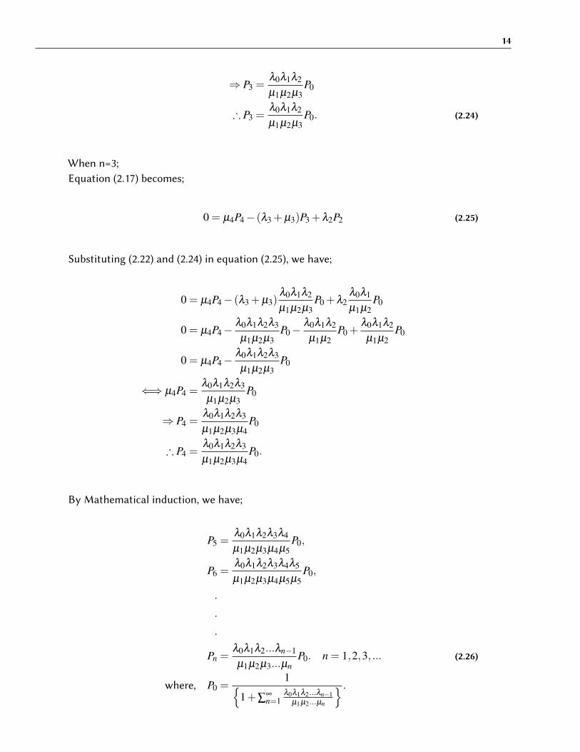
14

⇒ P3 =λ0λ1λ2

µ1µ2µ3P0

∴ P3 =λ0λ1λ2

µ1µ2µ3P0. (2.24)


0 = µ4P4− (λ3 +µ3)P3 +λ2P2 (2.25)


0 = µ4P4− (λ3 +µ3)λ0λ1λ2

µ1µ2µ3P0 +λ2

λ0λ1

µ1µ2P0

0 = µ4P4−λ0λ1λ2λ3

µ1µ2µ3P0−

λ0λ1λ2

µ1µ2P0 +

λ0λ1λ2

µ1µ2P0

0 = µ4P4−λ0λ1λ2λ3

µ1µ2µ3P0

⇐⇒ µ4P4 =λ0λ1λ2λ3

µ1µ2µ3P0

⇒ P4 =λ0λ1λ2λ3

µ1µ2µ3µ4P0

∴ P4 =λ0λ1λ2λ3

µ1µ2µ3µ4P0.

By Mathematical induction, we have;

P5 =λ0λ1λ2λ3λ4

µ1µ2µ3µ4µ5P0,

P6 =λ0λ1λ2λ3λ4λ5

µ1µ2µ3µ4µ5µ5P0,

.

.

.


µ1µ2µ3...µnP0. n = 1,2,3, ... (2.26)

where, P0 =1{

1+∑∞n=1

λ0λ1λ2...λn−1µ1µ2...µn

} .

15

But;

∞

∑n=0

Pn = 1

⇒ P0 +P1 +P2 +P3 + ...+Pn + ...= 1

P0 +λ0

µ1P0 +

λ0λ1

µ1µ2P0 +

λ0λ1λ2

µ1µ2µ3P0 + ...+

λ0λ1λ2...λn−1

µ1µ2µ3...µnP0 + ...= 1

P0

{1+

λ0

µ1+

λ0λ1

µ1µ2+

λ0λ1λ2

µ1µ2µ3+ ...+

λ0λ1λ2...λn−1

µ1µ2µ3...µn+ ...

}= 1

P0

{1+

∞

∑n=1

λ0λ1λ2...λn−1

µ1µ2µ3...µn

}= 1

Thus, the probability of ultimate extinction is given by;

P0 =1{

1+∑∞n=1

λ0λ1λ2...λn−1µ1µ2µ3...µn

} .

Therefore;

Pn =

λ0λ1λ2...λn−1µ1µ2µ3...µn{

1+∑∞n=1

λ0λ1λ2...λn−1µ1µ2µ3...µn

} ; n = 1,2,3, ... (2.27)

2.4 Recursive Relation based on two consecutive terms

Proposition 2.2

Pn

Pn−1=

λn−1

µn, µn 6= 0 (2.28)

ProofFrom (2.26), we have;

16


µ1µ2µ3...µnP0. n = 1,2,3, ...

⇒ Pn−1 =λ0λ1λ2...λn−2

µ1µ2µ3...µn−1P0.

Therefore,

Pn

Pn−1=

λ0λ1λ2...λn−2λn−1

µ1µ2µ3...µn−1µn.µ1µ2µ3...µn−1

λ0λ1λ2...λn−2

∴Pn

Pn−1=

λn−1

µn, µn 6= 0 (2.29)

2.5 Problem Statement

The problem is to determine Pn using propositions (2.1) and (2.2). For special cases, di�er-ential equations in probability generating function will be derived and solved to obtainthe means and the variance.

2.6 Population Growth Model

Note that, from (2.11) the basic di�erence di�erential equations for the general Birth-and-Death processes at equilibrium are:

0 = µ1P1−λ0P0,

0 = µn+1Pn+1 +λn−1Pn−1− (λn +µn)Pn; n≥ 1

2.7 Birth, Death and Immigration Process

One interesting variant of simple Birth-and-Death Process is obtained if we add thecondition that in an infinititesimal time interval ∆t, there is a chance v∆t +0(∆t) that asingle member will be added to the population by immigration from the outside world.The characteristic feature of immigration e�ect is that it acts at an expected rate which isindependent of the population size.Here,

17

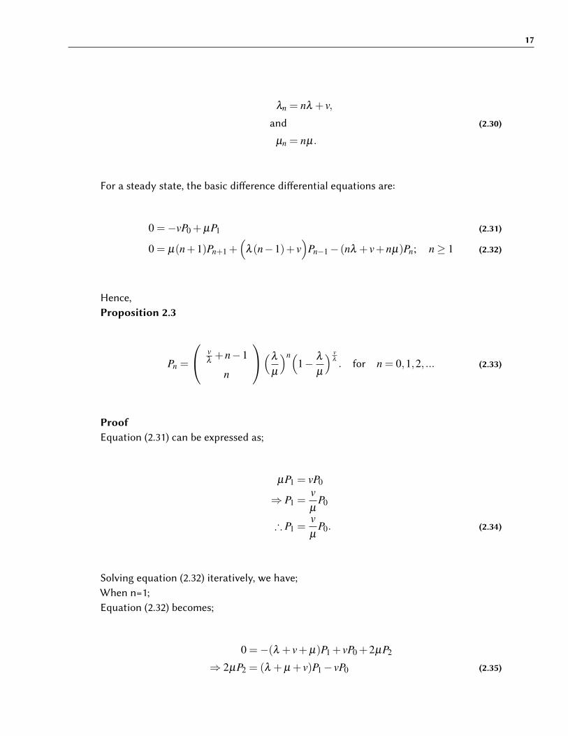
λn = nλ + v,

and (2.30)

µn = nµ.

For a steady state, the basic di�erence di�erential equations are:

0 =−vP0 +µP1 (2.31)

0 = µ(n+1)Pn+1 +(

λ (n−1)+ v)

Pn−1− (nλ + v+nµ)Pn; n≥ 1 (2.32)

Hence,Proposition 2.3

Pn =

vλ+n−1

n

(λ

µ

)n(1− λ

µ

) vλ

. for n = 0,1,2, ... (2.33)


µP1 = vP0

⇒ P1 =vµ

P0

∴ P1 =vµ

P0. (2.34)

Solving equation (2.32) iteratively, we have;When n=1;Equation (2.32) becomes;

0 =−(λ + v+µ)P1 + vP0 +2µP2

⇒ 2µP2 = (λ +µ + v)P1− vP0 (2.35)

18

Substituting (2.34) in equation (2.35), we get;

2µP2 = (λ +µ + v)vµ

P0− vP0

=(vλ + v2

µ

)P0

=vµ(λ + v)P0

⇒ P2 =v

2µ2 (λ + v)P0

∴ P2 =v

2µ2 (λ + v)P0. (2.36)


0 =−(2λ + v+2µ)P2 +(λ + v)P1 +3µP3 (2.37)

Substituting (2.34) and (2.36) in equation (2.37), we get;

0 =−(2λ + v+2µ)v

2µ2 (λ + v)P0 +(λ + v)vµ

P0 +3µP3

0 =−vλ

µ2 (λ + v)P0−v2

2µ2 (λ + v)P0−vµ(λ + v)P0 +

vµ(λ + v)P0 +3µP3

0 =−vλ

µ2 (λ + v)P0−v2

2µ2 (λ + v)P0 +3µP3

⇐⇒ 3µP3 =v(λ + v)(2λ + v)

µ.2µ2.µ2 P0

⇒ P3 =v(λ + v)(2λ + v)

µ.2µ2.3µ3 P0

∴ P3 =v(λ + v)(2λ + v)

µ.2µ2.3µ3 P0.

19

Therefore,

P4 =v(λ + v)(2λ + v)(3λ + v)

µ.2µ2.3µ3.4µ4 P0,

P5 =v(λ + v)(2λ + v)(3λ + v)(4λ + v)

µ.2µ2.3µ3.4µ4.5µ5 P0,

.

.

.

Pn =n−1

∏j=0

jλ + vn!µn P0. (2.38)

=P0

n!µn

n−1

∏j=0

( jλ + v)

=P0

n!µn

n−1

∏j=0

λ ( j+vλ)

=P0λ n

n!µn

n−1

∏j=0

( j+vλ)

=P0

n!

(λ

µ

)n{ vλ(

vλ+1)(

vλ+2)...(

vλ+n−1)

}=

P0

n!

(λ

µ

)n{(

vλ+n−1)(

vλ+n−2)...(

vλ+1)

vλ

}=

P0

n!

(λ

µ

)n{(

vλ+n−1)(

vλ+n−2)...(

vλ+1)

vλ

Γ( vλ)

Γ( vλ)

}=

P0

n!

(λ

µ

)n{(

vλ+n−1)(

vλ+n−2)...(

vλ+1)

Γ( vλ+1)

Γ( vλ)

}=

P0

n!

(λ

µ

)n 1Γ( v

λ)

{(

vλ+n−1)(

vλ+n−2)...(

vλ+2)Γ(

vλ+2)

}.

.

.

∴ Pn =P0

n!

(λ

µ

)n 1Γ( v

λ)

{(

vλ+n−1)Γ(

vλ+n−1)

}Pn = P0

(λ

µ

)n 1n!Γ( v

λ)Γ(

vλ+n)

20

Therefore,

Pn = P0

(λ

µ

)n Γ( vλ+n)

n!Γ( vλ)

= P0

(λ

µ

)n

vλ+n−1

n

∴ Pn =

vλ+n−1

n

(λ

µ

)nP0; n = 1,2,3, ... (2.39)

But;

∞

∑n=0

Pn = 1

⇒ P0 +P1 +P2 + ...= 1

P0 +vµ

P0 +v

2µ2 (λ + v)P0 + ...= 1

P0{1+ vµ+

v2µ2 (λ + v)+ ...}= 1

∴ P0 = (1− λ

µ)

vλ . (2.40)

∴ Pn =

vλ+n−1

n

(λ

µ

)n(1− λ

µ)

vλ ; n = 0,1,2,3, ...

(2.41)

This is a Negative Binomial Distribution with parameters vλ

and 1− λ

µ.

Remark (2.1)

(1) In the birth, death and immigration processes, the population either remain con-stant, increase or decrease.It may eventually reach zero; however, since there is always a positive immigration ratev, the population will never become extinct. But the population will become extinct as vgoes to zero.i.e., limv→∞ Pn.

Using Proposition 2.1

21

We have;

Pn =λ0λ1λ2λ3...λn−1

µ1µ2µ3...µnP0

But, λ0 = v, λ1 = λ + v, λ2 = (2λ + v), λ3 = (3λ + v), ..., λn−1 = (n−1)λ + v.

and

µ1 = µ, µ2 = 2µ, µ3 = 3µ, ..., µn = nµ.

∴ Pn =v(λ + v)(2λ + v)...[(n−1)λ + v]

µ2µ3µ...nµP0

=v(λ + v)(2λ + v)...[(n−1)λ + v]

n!µn P0

=n−1

∏j=0

jλ + vn!µn P0

=P0

n!µn

n−1

∏j=0

( jλ + v)

=P0

n!µn

n−1

∏j=0

λ ( j+vλ)

=P0λ n

n!µn

n−1

∏j=0

( j+vλ)

=P0

n!

(λ

µ

)n{ vλ(

vλ+1)(

vλ+2)...(

vλ+n−1)

}=

P0

n!

(λ

µ

)n{(

vλ+n−1)(

vλ+n−2)...(

vλ+1)

vλ

}=

P0

n!

(λ

µ

)n{(

vλ+n−1)(

vλ+n−2)...(

vλ+1)

vλ

Γ( vλ)

Γ( vλ)

}=

P0

n!

(λ

µ

)n{(

vλ+n−1)(

vλ+n−2)...(

vλ+1)

Γ( vλ+1)

Γ( vλ)

}

∴ Pn =P0

n!

(λ

µ

)n 1Γ( v

λ)

{(

vλ+n−1)(

vλ+n−2)...(

vλ+2)Γ(

vλ+2)

}.

.

.

Pn =P0

n!

(λ

µ

)n 1Γ( v

λ)

{(

vλ+n−1)(

vλ+n−2)Γ(

vλ+n−2)

}

22

Therefore,

Pn =P0

n!

(λ

µ

)n 1Γ( v

λ)

{(

vλ+n−1)Γ(

vλ+n−1)

}= P0

(λ

µ

)n 1n!Γ( v

λ)Γ(

vλ+n)

= P0

(λ

µ

)n Γ( vλ+n)

n!Γ( vλ)

= P0

(λ

µ

)n

vλ+n−1

n

∴ Pn =

vλ+n−1

n

(λ

µ

)nP0; n = 1,2,3, ...

But,

∞

∑n=0

Pn = 1

i.e., P0 +∞

∑n=0

Pn = 1

P0[1+∞

∑n=1

vλ+n−1

n

(λ

µ

)n] = 1

P0

∞

∑n=0

vλ+n−1

n

(λ

µ

)n= 1

P0

∞

∑n=0

(−1)n

− vλ

n

(λ

µ

)n= 1

23

Therefore,

P0

∞

∑n=0

− vλ

n

(− λ

µ

)n= 1

∴ P0(1−λ

µ)−

vλ = 1

∴ P0 = (1− λ

µ)−

vλ .

∴ Pn =

vλ+n−1

n

(λ

µ

)n(1− λ

µ)

vλ ; n = 0,1,2,3, ...

Which is a Negative Binomial Distribution with parameters vλ

and 1− λ

µ.

where, λ < µ, λ > 0, µ > 0.

Using Proposition 2.2

Pn

Pn−1=

λn−1

µn, µn 6= 0

But,

λn−1 = (n−1)λ + v,

and

µn = nµ.

Therefore,

Pn

Pn−1=

(n−1)λ + vnµ

=(n−1+ v

λ)

nµ

λ

∴Pn

Pn−1= (

vλ+n−1)

λ

µ

n

∴Pn

Pn−1= (

vλ+n−1)

λ

µ

n.

⇒ nPn =λ

µ(

vλ+n−1)Pn−1; n = 1,2,3, ... (2.42)

24

Using the probability generating function technique, we multiply (2.42) by sn and sum theresults over n to obtain;

∞

∑n=1

nPnsn =λ

µ

∞

∑n=1

(vλ+n−1)Pn−1sn

∞

∑n=1

nPnsn =λ

µ.vλ

∞

∑n=1

Pn−1sn +λ

µ

∞

∑n=1

(n−1)Pn−1sn

s∞

∑n=1

nPnsn−1 =λ

µ.vλ

s∞

∑n=1

Pn−1sn−1 +λ

µs2

∞

∑n=1

(n−1)Pn−1sn−1

sψ(s)

ds=

λ

µ.vλ

sψ(s)+λ

µs2 dψ(s)

ds

⇐⇒ (1− λ

µs)

dψ(s)ds

=λ

µ.vλ

sψ(s)

⇒ dψ(s)ψ(s)

=

λ

µ. v

λ

(1− λ

µs)

ds

Integrating both sides, we have;

∫ dψ(s)ψ(s)

=∫ λ

µ. v

λ

(1− λ

µs)

ds

lnψ(s) =− vλ

ln(1− λ

µs)+ lnc

∴ ψ(s) = c1(1−λ

µs)−

vλ .

Pu�ing s=1;

ψ(1) = 1 = c1(1−λ

µ)−

vλ

⇒ c1 = (1− λ

µ)

vλ .

∴ ψ(s) = (1− λ

µ)

vλ (1− λ

µs)−

vλ

25

∴ ψ(s) =( (1− λ

µ)

(1− λ

µs)

) vλ

. (2.43)

Which is the pgf. for a Negative Binomial Distribution with parametersvλ

and 1− λ

µ.

ψ′(s) =

λ

µ

vλ(1− λ

µ)

vλ

(1− λ

µs)

vλ+1

ψ′′(s) =

(λ

µ)2. v

λ( v

λ+1)(1− λ

µ)

vλ

(1− λ

µs)

vλ+2

=(λ

µ)2( v

λ)2(1− λ

µ)

vλ +(λ

µ)2 v

λ(1− λ

µ)

vλ

(1− λ

µs)

vλ+2

E(X) = ψ(1) =λ

µ

vλ(1− λ

µ)

vλ

(1− λ

µ)

vλ+1

∴ E(X) =v

µ−λ.

The variance is given by;

Var(X) = ψ′′(1)+ψ

′(1)− [ψ

′(1)]2

=(λ

µ)2( v

λ)2(1− λ

µ)

vλ +(λ

µ)2 v

λ(1− λ

µ)

vλ

(1− λ

µ)

vλ+2 +

λ

µ

vλ(1− λ

µ)

vλ

(1− λ

µ)

vλ+1 − [

λ

µ

vλ(1− λ

µ)

vλ

(1− λ

µ)

vλ+1 ]2

=(λ

µ)2( v

λ)2(1− λ

µ)

vλ +(λ

µ)2 v

λ(1− λ

µ)

vλ

(1− λ

µ)

vλ+2 +

λ

µ

vλ(1− λ

µ)

vλ

(1− λ

µ)

vλ+1 −

(λ

µ)2( v

λ)2

(1− λ

µ)2

=(λ

µ)2( v

λ)2 +(λ

µ)2 v

λ

(1− λ

µ)2

+

λ

µ

vλ

(1− λ

µ)−

(λ

µ)2( v

λ)2

(1− λ

µ)2

=vλ + vµ− vλ

(µ−λ )2

∴Var(X) =vµ

(µ−λ )2 .

26

From Gauss hypergeometric series, we have;

2F1(vλ,1;1;

λ

µ) = 1+

vλ.11

λ

µ

1!+

vλ( v

λ+1)1(1+1)1(1+1)

(λ

µ)2

2!+ ...+

( vλ+n−1)(1+n−1)

(1+n−1)

(λ

µ)n

n!

=∞

∑n=0

vλ( v

λ+1)...( v

λ+n−1)1(1+1)(1+2)...(1+n−1)

1(1+1)(1+2)...(1+n−1)

(λ

µ)n

n!

=∞

∑n=0

( vλ+n−1)...( v

λ+1) v

λ(1+n−1)...(1+2)(1+1)1

(1+n−1)...(1+2)(1+1)1

(λ

µ)n

n!

=∞

∑n=0

Γ( vλ+n)Γ(1+n)Γ(1+n)

.Γ(1)

Γ( vλ)Γ(1)

(λ

µ)n

n!

Normalizing, we get;

1 =∞

∑n=0


.Γ(1)

Γ( vλ)Γ(1)

.1

2F1(vλ,1;1; λ

µ)

(λ

µ)n

n!

Hence,

Pn = Prob.(N = n)

=Γ( v

λ+n)Γ(1+n)Γ(1+n)

.Γ(1)

Γ( vλ)Γ(1)

.1

2F1(vλ,1;1; λ

µ)

(λ

µ)n

n!

The pgf. in hypergeometric terms is given by;

φ(z) =∞

∑n=0

Pnzn

φ(z) =∞

∑n=0


.Γ(1)

Γ( vλ)Γ(1)

(λ

µz)n

n!.

1

2F1(vλ,1;1; λ

µ)

∴ φ(z) =2F1(

vλ,1;1; λ

µz)

2F1(vλ,1;1; λ

µ).

φ′(z) =

vλ

λ

µ

2F1(vλ+1,1+1;1+1; λ

µz)

2F1(vλ,1;1; λ

µ)

φ′′(z) =

vλ(

vλ+1)(

λ

µ)2 2F1(

vλ+2,3;3; λ

µz)

2F1(vλ,1;1; λ

µ)

27

Therefore,

Let, Λκ =2F1(

vλ+κ,1+κ;1+κ; λ

µ)

2F1(vλ,1;1; λ

µ)

; κ = 1,2.

E(X) = φ′(1)

∴ E(X) =vλ

λ

µΛ1.

Var(X) = φ′′(1)+φ

′(1)− [φ

′(1)]2.

=vλ(

vλ+1)(

λ

µ)2

Λ2 +vλ

λ

µΛ1− [

vλ

λ

µΛ1]

2

∴Var(X) =vλ

λ

µΛ1 +

vλ(λ

µ)2{( v

λ+1)Λ2−

vλ

Λ21}.

3 BIRTH AND DEATH PROCESSES AT EQUILIBRIUMWITH APPLICATION TO WAITING LINEPROBLEMS

3.1 Introduction

In this chapter, birth and death processes and some special cases of waiting line and ser-vicing problems are explored. Their basic di�erence di�erential equations at equilibriumare stated given di�erent birth λn and death µn rate values or functions.The steady states equations are solved iteratively to generate distributions arising fromthe birth and death process. Some properties and special cases of these distributions havealso been discussed.

3.2 The simple trunking problem

Suppose that infinitely many trunks or channels are available, and that the probabilityof a conversation ending between t and t +∆t is µ∆t +0(∆t), (exponential holding time).The incoming calls constitute a tra�ic of the Poisson type with parameter λ .Assume that the duration of conversations are mutually independent. If n lines are busy,the probability that one of them will be free within time ∆t is then nµ∆t+)(∆t). Theprobability of a new call arriving is λ∆t + 0(∆t). The probability of a combination ofseveral calls, or of a call arriving and a conversation ending is 0(∆t).Thus, this implies that;

λn = λ ,

and

µn = nµ.

At a stedy state, t→ ∞ implying that Pn(t) is independent of t.Thus,

30

Pn(t) = Pn,

and

limt→∞

P′n(t) = 0.

Therefore, the basic di�erence di�erential equations for the steady state for the simpletrunking problem are:

0 = µP1−λP0 (3.1)

0 = (n+1)µPn+1 +(n−1)λPn−1− (λ +nµ)Pn, n≥ 1 (3.2)


Pn =λ n

n!µn e−λ

µ (3.3)


λP0 = µP1

⇒ λ

µP0 = P1

∴ P1 =λ

µP0. (3.4)

Solving steady state equation iteratively, we have;When n=1;Equation (3.2) becomes;

0 = 2µP2 +λP0− (λ +µ)P1 (3.5)

31


0 = 2µP2 +λP0− (λ +µ)λ

µP0

0 = 2µP2 +λP0−λP0−λ 2

µP0

0 = 2µP2−λ 2

µP0

⇐⇒ λ 2

µP0 = 2µP2

⇒ λ 2

2!µ2 P0 = P2

∴ P2 =λ 2

2!µ2 P0. (3.6)


0 = 3µP3 +λP1− (λ +2µ)P2 (3.7)


0 = 3µP3 +λλ

µP0− (λ +2µ)

λ 2

2!µ2 P0

0 = 3µP3 +λ 2

µP0−

λ 2

µP0−

λ 3

2µ2 P0

0 = 3µP3−λ 3

2µ2 P0

⇐⇒ λ 3

2µ2 P0 = 3µP3

⇒ λ 3

3!µ3 P0 = P3

∴ P3 =λ 3

3!µ3 P0. (3.8)


32

0 = 4µP4 +λP2− (λ +3µ)P3 (3.9)


0 = 4µP4 +λλ 2

2!µ2 P0− (λ +3µ)λ 3

3!µ3 P0

0 = 4µP4 +λ 3

2µ2 P0−λ 3

2µ2 P0−λ 4

3!µ3 P0

0 = 4µP4−λ 4

3!µ3 P0

⇐⇒ λ 4

3!µ3 P0 = 4µP4

⇒ λ 4

4!µ4 P0 = P4

∴ P4 =λ 4

4!µ4 P0.

Therefore,

P5 =λ 5

5!µ5 P0,

P6 =λ 6

6!µ6 P0,

.

.

.

Pn =λ n

n!µn P0. (3.10)

.

.

.

But,

∞

∑n=0

Pn = 1

33

⇒ P0

{1+

λ

µ+

λ 2

2!µ2 +λ 3

3!µ3 +λ 4

4!µ4 + ...}= 1

P0

{e

λ

µ

}= 1

∴ P0 = e−λ

µ . (3.11)

Hence,

P1 =λ

1!µe−

λ

µ ,

P2 =λ 2

2!µ2 e−λ

µ ,

P3 =λ 3

3!µ3 e−λ

µ ,

P4 =λ 4

4!µ4 e−λ

µ ,

.

.

.

We find by Mathematical induction that;

Pn =λ n

n!µn e−λ

µ . (3.12)

Thus, the limiting distribution is a Poisson with parameter λ

µ. It is independent of the

initial state.Using Proposition (2.1)We have;


µ1µ2µ3...µnP0

But, λ0 = λ1 = λ2 = λ3 = ...= λn−1 = λ ,

and

µ1 = µ, µ2 = 2µ, µ3 = 3µ, ..., µn = nµ.

∴ Pn =λλλλ ...λ

µ2µ3µ...nµP0

34

Therefore,

Pn =λ n

n!µn P0

But, from (3.11) above;

P0 = e−λ

µ

∴ Pn =λ n

n!µn e−λ

µ .

Which is a Poisson distribution with parameter λ

µ.

Using Proposition (2.2)

Pn

Pn−1=

λn−1

µn, µn 6= 0

But, λn−1 = λ ,

and

µn = nµ.

∴Pn

Pn−1=

λ

nµ.

Proposition 3.2

Pn

Pn−1=

λ

nµ

⇒ nµPn = λPn−1 (3.13)

Multiplying (3.13) by sn and sum the results over n we obtain;

∞

∑n=0

nµPnsn =∞

∑n=0

λPn−1sn

µs∞

∑n=0

nPnsn−1 = λ s∞

∑n=0

Pn−1sn−1

sµdψ(s)

ds= sλψ(s)

dψ(s)ψ(s)

=λ

µds

35


∫ dψ(s)ψ(s)

=∫

λ

µds

lnψ(s) =λ

µs+ c

ψ(s) = c1eλ

µs

Pu�ing s=1;

ψ(1) = 1 = c1eλ

µ

⇒ c1 = e−λ

µ .

∴ ψ(s) = e−λ

µ eλ

µs

∴ ψ(s) = e−λ

µ(1−s).

Which is the pgf. for a Poisson distribution with parameter λ

µ.

ψ′(s) =

λ

µe−

λ

µ(1−s)

ψ′′(s) = (

λ

µ)2e−

λ

µ(1−s)

E(X) = ψ′(1)

∴ E(X) =λ

µ.

Var(x) = ψ′′(1)+ψ

′(1)− [ψ

′(1)]2

= (λ

µ)2 +

λ

µ− [

λ

µ]2

∴Var(X) =λ

µ.

36

From Kummer’s confluent hypergeometric series, we have;

1F1([;[;λ

µ) = 1+

[

[

λ

µ

1!+

[([+1)[([+1)

(λ

µ)2

2!+ ...+

([+n−1)([+n−1)

(λ

µ)n

n!

=∞

∑n=0

[([+1)([+2)...([+n−1)[([+1)([+2)...([+n−1)

(λ

µ)n

n!

=∞

∑n=0

([+n−1)([+n−2)...([+2)([+1)[([+n−1)([+n−2)...([+2)([+1)[

Γ([)

Γ([).Γ([)

Γ([).(λ

µ)n

n!

=∞

∑n=0

Γ([+n)Γ([+n)

Γ([)

Γ([).(λ

µ)n

n!

Normalizing, we have;

1 =∞

∑n=0

Γ([+n)Γ([+n)

Γ([)

Γ([).

1

1F1([;[; λ

µ)

(λ

µ)n

n!

Therefore,

Pn = Prob.(N = n)

=Γ([+n)Γ([+n)

Γ([)

Γ([).

1

1F1([;[; λ

µ)

(λ

µ)n

n!

In hypergeometric terms, its pgf. is given as;

φ(z) =∞

∑n=0

Pnzn

=Γ([+n)Γ([+n)

Γ([)

Γ([)

(λ

µz)n

n!.

1

1F1([;[; λ

µ)

∴ φ(z) =1F1([;[; λ

µz)

1F1([;[; λ

µ).

φ′(z) =

λ

µ

1F1([+1;[+1; λ

µz)

1F1([;[; λ

µ)

φ′′(z) = (

λ

µ)2 1F1([+2;[+2; λ

µz)

1F1([;[; λ

µ)

37

Therefore,

Let, Λκ =1F1([+κ;[+κ; λ

µ)

1F1([;[; λ

µ)

; κ = 1,2.

∴ E(x) =λ

µΛ1.

Var(X) = φ′′(1)+φ

′(1)− [φ

′(1)]2

= (λ

µ)2

Λ2 +λ

µΛ1− (

λ

µ)2

Λ21

∴Var(X) =λ

µΛ1 +(

λ

µ)2(Λ2−Λ

21).

3.3 Waiting lines for a finite number of channels

Assume that the number of channels is finite and equals to k. If all channels are busy,each new call joins a waiting line and wait until a channel is free.We say that the system is in a state En if there are n persons either being served or in thewaiting line. Such a line exists only when, n > k and there are n− k persons in it.As long as at least one channel is free then,

λn = λ ,

and

µn = nµ; for n < k.

However, if n > k, only k conversations are going on and λn = kµ ; for n≥ k.The basic di�erence di�erential equations for the steady state for waiting lines for a finitenumber of channels are:

0 = µP1−λP0 (3.14)

0 = (n+1)µPn+1 +λPn−1− (λ +nµ)Pn; for n < k (3.15)

0 = kµPn+1 +λPn−1− (λ + kµ)Pn; n≥ k (3.16)

38

Proposition 3.3

Pn =(λ

µ)n

k!kn−1 e−λ

µ ; for n≥ k; forλ

µ< k. (3.17)

ProofSolving the steady state equations iteratively, we have;Equation (3.14) can be expressed as;

λP0 = µP1

⇒ λ

µP0 = P1

∴ P1 =λ

µP0 (3.18)


0 = 2µP2 +λP0− (λ +µ)P1 (3.19)


0 = 2µP2 +λP0− (λ +µ)λ

µP0

0 = 2µP2 +λP0−λP0−λ 2

µP0

0 = 2µP2−λ 2

µP0

⇐⇒ λ 2

µP0 = 2µP2

⇒ λ 2

2!µ2 P0 = P2

∴ P2 =λ 2

2!µ2 P0. (3.20)

39


0 = 3µP3 +λP1− (λ +2µ)P2 (3.21)


0 = 3µP3 +λλ

µP0− (λ +2µ)

λ 2

2!µ2 P0

0 = 3µP3 +λ 2

µP0−

λ 2

µP0−

λ 3

2µ2 P0

0 = 3µP3−λ 3

2µ2 P0

⇐⇒ λ 3

2!µ2 P0 = 3µP3

⇒ λ 3

3!µ3 P0 = P3

∴ P3 =λ 3

3!µ3 P0.

Hence,

P4 =λ 4

4!µ4 P0,

P5 =λ 5

5!µ5 P0,

.

.

.

Pn =λ n

n!µn P0. (3.22)

.

.

.

40

Note that;

∞

∑n=0

Pn = 1

⇒ P0 +(λ

µ)1

1!P0 +

(λ

µ)2

2!P0 +

(λ

µ)3

3!P0 +

(λ

µ)4

4!P0 + ...+ ...= 1

P0

{1+

(λ

µ)1

1!+

(λ

µ)2

2!+

(λ

µ)3

3!+

(λ

µ)4

4!+ ...+ ...

}= 1

P0(eλ

µ ) = 1

∴ P0 = e−λ

µ . (3.23)

Thus;

P1 =λ 1

1!µ1 e−λ

µ ,

P2 =λ 2

2!µ2 e−λ

µ ,

P3 =λ 3

3!µ3 e−λ

µ ,

P4 =λ 4

4!µ4 e−λ

µ ,

.

.

.

∴ Pn =λ n

n!µn e−λ

µ .


µ.

Next,When n=1;Equation (3.16) becomes;

0 = kµP2 +λP0− (λ + kµ)P1 for n≥ k (3.24)

41


0 = kµP2 +λP0− (λ + kµ)λ

µP0

0 = kµP2 +λP0− kλP0−λ 2

µP0

0 = kµP2−λ (1− k)P0−λ 2

µP0

⇐⇒ λ (1− k)P0 +λ 2

µP0 = kµP2

⇒ 1k

(λ

µ(1− k)+

λ 2

µ2

)P0 = P2

∴ P2 =1k

(λ

µ(1− k)+

λ 2

µ2

)P0. (3.25)


0 = kµP3 +λP1− (λ + kµ)P2 for n≥ k (3.26)

Substituting (3.18) and 3.25) in equation (3.26), we get;

0 = kµP3 +λ 2

µP0− (λ + kµ)

1k

(λ

µ(1− k)+

λ 2

µ2

)P0

⇐⇒ λ 3

kµ2 P0 +λ 2

kµ(k−1)P0 +λ (k−1)P0 = kµP3

⇒ 1k2

(λ 3

µ3 +λ 2

µ2 (k−1)+λ

µk(k−1)

)P0 = P3

∴ P3 =1k2

(λ 3

µ3 +λ 2

µ2 (k−1)+λ

µk(k−1)

)P0.

42

Hence,

P4 =1k3

(λ 4

µ4 +λ 3

µ3 (k−1)+λ 2

µ2 k(k−1)+λ

µK(k−1)(k−2)

)P0,

.

.

.

Pn =1

kn−k

(λ n

µn +λ n−1

µn−1 (k−1)+ ...λ

µk(k−1)(k−2)...(k−n)

)P0.

for n≥ k.

Assume that λ

µ< k.

But,

∞

∑n=0

Pn = 1 for n≥ k.

⇒ P0

(1+

λ

1!µ+(

1k)−1 λ 2

2!µ2 + ...+(1

kn−1 )−1 λ n

k!µn + ...)= 1

P0

((

1kn−1 )

−1eλ µ

)= 1

⇒ P0kn−k =1

eλ

µ

∴ P0 =1

kn−k e−λ

µ .

Thus,

Pn =(λ

µ)n

k!kn−1 P0.

∴ Pn =(λ

µ)n

k!kn−1 e−λ

µ ; for n≥ k; forλ

µ< k.

Remark 3.1The series ∑(Pn

P0) converge only if λ

µ< k i.e., ∑Pn = 1. If λ

µ≥ k, a limiting distribution

Pn cannot exists.In this case, Pn = 0 for all n, which means that gradually the waiting line grow over allbounds.

43

3.4 Servicing of machines by a single repairman

We consider ξ automatic machines which call for service only in the event of breakdown.Let λ∆t + 0(∆t) be the probability of calling for service in time ∆t if it is working at t(time) and µ∆t +0(∆t) be the probability of machine reverting back to work if it is beingserviced at t .Let the system be in state En when n machines are working. A transition En → En+1

is caused by breaking of one of the working machines, while a transition En→ En−1 iscaused by the return to work of a machine being serviced.Thus, we have a Birth and Death process with coe�icients:

λn = (ξ −n)λ ,

and

µ0 = 0, µ1 = µ2 = ...= µξ = µ; for 1≤ n≤ ξ −1.

The basic di�erence di�erential equations for the steady state problem for servicing ofmachines with only one repairman are:

0 =−ξ λP0 (3.27)

0 =−{(ξ −n)λ +µ}Pn +(ξ −n+1)λPn−1 +µPn+1 (3.28)

0 =−µPξ +λPξ−1 (3.29)


Pξ ={

1+11!(λ

µ)1 +

12!(λ

µ)2 +

13!(λ

µ)3 +

14!(λ

µ)4 + ...+

1ξ !

(λ

µ)ξ

}−1(3.30)

ProofSolving the steady state equations iteratively, we get;Equation (3.27) can be expresses as;

44

µP1 = ξ λP0

⇒ P1 = ξλ

µP0

∴ P1 = ξλ

µP0. (3.31)


0 =−{(ξ −1)λ +µ}P1 +ξ λP0 +µP2 (3.32)


0 =−{(ξ −1)λ +µ}ξ λ

µP0 +ξ λP0 +µP2

0 =−ξ 2λ 2

µP0 +

ξ λ 2

µP0−ξ λP0 +ξ λP0 +µP2

0 =−ξ 2λ 2

µP0 +

ξ λ 2

µP0 +µP2

0 =−λ 2

µξ (ξ −1)P0 +µP2

⇐⇒ µP2 =λ 2

µξ (ξ −1)P0

⇒ P2 =λ 2

µ2 ξ (ξ −1)P0

∴ P2 =λ 2

µ2 ξ (ξ −1)P0. (3.33)


0 =−{(ξ −2)λ +µ}P2 +(ξ −1)λP1 +µP3 (3.34)

45


0 =−{(ξ −2)λ +µ}λ 2

µ2 ξ (ξ −1)P0 +(ξ −1)λξλ

µP0 +µP3

0 =−λ 3

µ2 ξ (ξ −1)(ξ −2)P0−λ 2

µξ (ξ −1)P0 +

λ 2

µξ (ξ −1)P0 +µP3

0 =−λ 3

µ2 ξ (ξ −1)(ξ −2)P0 +µP3

⇐⇒ µP3 =λ 3

µ2 ξ (ξ −1)(ξ −2)P0

⇒ P3 =λ 3

µ3 ξ (ξ −1)(ξ −2)P0

∴ P3 =λ 3

µ3 ξ (ξ −1)(ξ −2)P0.

Hence;

P4 =λ 4

µ4 ξ (ξ −1)(ξ −2)(ξ −3)P0,

P5 =λ 5

µ5 ξ (ξ −1)(ξ −2)(ξ −3)(ξ −4)P0,

.

.

.

∴ Pn =λ n

µn ξ (ξ −1)(ξ −2)(ξ −3)...(ξ −n)P0. (3.35)

Note that;

ξ (ξ −1)(ξ −2)(ξ −3)...(ξ −ξ ) = { 1ξ}−1

⇒ P1 = {11!}−1(

λ

µ)1P0,

P2 = {12!}−1(

λ

µ)2P0,

∴ P3 = {13!}−1(

λ

µ)3P0,

46

Therefore,

P4 = {14!}−1(

λ

µ)4P0,

.

.

.

Pξ = { 1ξ !}−1(

λ

µ)ξ P0.

Therefore,

Pξ ={

1+11!(λ

µ)1 +

12!(λ

µ)2 +

13!(λ

µ)3 +

14!(λ

µ)4 + ...+

1ξ !

(λ

µ)ξ

}−1.

Which is Erlang’s loss function.

P0 =1ξ(

µ

λ)ξ Pξ .

Which gives the probability of a repairman being idle.We find by Mathematical induction that;

P0 = (1ξ)−1(

µ

λ)ξ Pξ .

Hence,

Pξ ={

1+11!(λ

µ)1 +

12!(λ

µ)2 +

13!(λ

µ)3 +

14!(λ

µ)4 + ...+

1ξ !

(λ

µ)ξ

}−1.

Thus, the limiting distribution is an Erlang distribution with parameter λ

µ.

It is independent of the initial condition, or equivalently the sum of independent exponen-tial distributions, or a gamma distribution of time Γ(ξ )e−

µ

λ .

The expected number of machines in the waiting line are:

47

ω =ξ

∑n=1

(n−1)Pn

∴ ω =ξ

∑n=1

nPn− (1−P0).

But,

(ξ −n)λPn = µPn+1,

∴ Pn =µ

λ (ξ −n)Pn+1.

3.5 Servicing of machines by several repairmen

Let ξ machines be serviced by r repairers (r < ξ ). Thus, for n ≤ r the state En meansr−n repair-men are idle while n machines are being serviced and no machines are in thewaiting line for repairs. In the case of n > r, the state En means r machines are beingserved and n− r machines are in the waiting line.Then set up is:

λ0 = ξ λ ; µ0 = 0

λn = (ξ −n)λ ; µn = nµ(1≤ n < r)

λn = (ξ −n)λ ; µn = rµ(r ≤ n < ξ ).

The basic di�erence di�erential equations for the steady state for servicing of machineswith several repairmen are:

0 =−ξ λP0 +µP1, for n = 0 (3.36)

0 =−{(ξ −n)λ +nµ}Pn +(ξ −n+1)λPn−1 +(n+1)µPn+1, (1≤ n < r) (3.37)

0 =−{(ξ −n)λ + rµ}Pn +(ξ −n+1)λPn−1 + rµPn+1, (r ≤ n < ξ ). (3.38)

48


Pn =

ξ

n

( λ

λ +µ

)n( µ

λ +µ

)ξ−n; n = 0,1,2, ...,ξ −1 (1≤ n < r). (3.39)


µP1 = ξ λP0

⇒ P1 = ξλ

µP0

∴ P1 = ξλ

µP0. (3.40)


0 =−{(ξ −1)λ +µ}P1 +ξ λP0 +2µP2 (3.41)


0 =−{(ξ −1)λ +µ}ξ λ

µP0 +ξ λP0 +2µP2

0 =−λ 2

µξ (ξ −1)−ξ λP0 +ξ λP0 +2µP2

0 =−λ 2

µξ (ξ −1)+2µP2

⇐⇒ 2µP2 =λ 2

µξ (ξ −1)+2µP2

⇒ P2 =λ 2

µ2 ξ (ξ −1)+2µP2

∴ P2 =λ 2

µ2 ξ (ξ −1)+2µP2. (3.42)

49


0 =−{(ξ −2)λ +2µ}P2 +(ξ −1)λP1 +3µP3 (3.43)


0 =−{(ξ −2)λ +2µ}λ 2

µ2 ξ (ξ −1)+2µP2 +(ξ −1)λξλ

µP0 +3µP3

0 =− λ 3

2µ2 ξ (ξ −1)(ξ −2)P0−λ 2

µξ (ξ −1)P0 +

λ 2

µξ (ξ −1)P0 +3µP3

0 =− λ 3

2µ2 ξ (ξ −1)(ξ −2)P0 +3µP3

⇐⇒ 3µP3 =λ 3

2µ2 ξ (ξ −1)(ξ −2)P0

⇒ P3 =λ 3

3!µ3 ξ (ξ −1)(ξ −2)P0

∴ P3 =λ 3

3!µ3 ξ (ξ −1)(ξ −2)P0.

Hence,

P4 =λ 4

4!µ4 ξ (ξ −1)(ξ −2)(ξ −3)P0,

P5 =λ 5

5!µ5 ξ (ξ −1)(ξ −2)(ξ −3)(ξ −4)P0,

.

.

.

Pn =λ n

n!µn ξ (ξ −1)(ξ −2)(ξ −3)...(r−n)P0. (3.44)

Let,

∑Pn = 1.

50

⇒ P1 =(

λ

µ

)1

ξ

1

P0,

P2 =(

λ

µ

)2

ξ

2

P0,

P3 =(

λ

µ

)3

ξ

3

P0,

.

.

.

But;

∞

∑n=0

Pn = 1

P0

{1+(

λ

µ

)1

ξ

1

+(

λ

µ

)2

ξ

2

+(

λ

µ

)3

ξ

3

+ ...}= 1

∴ P0 =(

µ

λ +µ

)n; n = 0,1,2, ...,ξ .

P0= The probability of machines not serviced.

Pn ={(

λ

λ +µ

)0(1− λ

λ +µ

)ξ

ξ

0

+(

λ

λ +µ

)1(1− λ

λ +µ

)ξ−1

ξ

1

+

(λ

λ +µ

)2(1− λ

λ +µ

)ξ−2

ξ

2

+ ...+(

λ

λ +µ

)n(1− λ

λ +µ

)ξ−n

ξ

n

}.∴ Pn =

{ ξ

n

( λ

λ +µ

)n(1− λ

λ +µ

)ξ−n}; n = 0,1,2, ...,ξ −1 (1≤ n < r).

(3.45)

Hence the limiting probabilities are given by the Binomial Distribution with parameters ξ

and λ

λ+µ.

51

Using Proposition 2.1We have;


µ1µ2µ3...µnP0

But, λ0 = ξ λ , λ1 = (ξ −1)λ , λ2 = (ξ −2)λ , λ3 = (ξ −3)λ , ...= λn−1 = (ξ − (n−1))λ .

and

µ1 = µ, µ2 = 2µ, µ3 = 3µ, ..., µn = nµ.

∴ Pn =ξ λ (ξ −1)λ (ξ −2)λ (ξ −3)λ ...(ξ − (n−1))λ

µ2µ3µ...nµP0

=ξ λ (ξ −1)λ (ξ −2)λ (ξ −3)λ ...(ξ − (n−1))λ

n!µn P0

=P0

n!µn

n−1

∏j=0

(ξ − j)λ

=λ nP0

n!µn

n−1

∏j=0

(ξ − j)

=P0

n!

(λ

µ

)n{ξ (ξ −1)(ξ −2)(ξ −3)...(ξ − (n−1))

}=

P0

n!

(λ

µ

)n{(ξ − (n−1))(ξ − (n−2))...(ξ −2)(ξ −1)ξ

}=

P0

n!

(λ

µ

)n{(ξ − (n−1))(ξ − (n−2))...(ξ −2)(ξ −1)ξ

Γ(ξ )

Γ(ξ )

}=

P0

n!

(λ

µ

)n{(ξ − (n−1))(ξ − (n−2))...(ξ −2)(ξ −1)

Γ(ξ −1)Γ(ξ )

}=

P0

n!

(λ

µ

)n 1Γ(ξ )

{(ξ − (n−1))(ξ − (n−2))...(ξ −2)Γ(ξ −2)

}=

P0

n!

(λ

µ

)n 1Γ(ξ )

{(ξ − (n−1))Γ(ξ − (n−1))

}= P0

(λ

µ

)n 1n!Γ(ξ )

Γ(ξ −n)

= P0

(λ

µ

)n Γ(ξ −n)n!Γ(ξ )

= P0

(1− λ

λ +µ

)ξ−n

ξ

n

52

∴ Pn =

ξ

n

(1− λ

λ +µ

)ξ−nP0 n = 0,1,2, ...

But,

∞

∑n=0

Pn = 1

i.e.,

P0

∞

∑n=0

ξ

n

(1− λ

λ +µ

)ξ−n= 1

P0

∞

∑n=0

(−1)n

−ξ

n

(1− λ

λ +µ

)ξ−n= 1

P0

∞

∑n=0

−ξ

n

( −λ

λ +µ

)ξ−n= 1

P0

(λ

λ +µ

)−n= 1

∴ P0 =(

λ

λ +µ

)n

∴ Pn =

ξ

n

(1− λ

λ +µ

)ξ−n( λ

λ +µ

)nn = 0,1,2, ...,ξ −1.

Which is a Binomial Distribution with parameters ξ and λ

λ+µ.

Let ξ = ξ and λ

λ+µ=ζ ;

Thus, the Binomial distribution becomes;

Pn =

ξ

n

(1−ζ

)ξ−n(ζ

)nn = 0,1,2, ...,ξ −1.

Then;Gauss hypergeometric series given by;

53

2F1(ξ , `;`;ζ ) = 1+ξ .`

1ζ

1!+

ξ (ξ +1)`(`+1)`(`+1)

(ζ )2

2!+ ...+

(ξ +n−1)(`+n−1)(`+n−1)

(ζ )n

n!

=∞

∑n=0

ξ (ξ +1)...(ξ +n−1)`(`+1)(`+2)...(`+n−1)`(`+1)(`+2)...(`+n−1)

(ζ )n

n!

=∞

∑n=0

(ξ +n−1)...(ξ +1)ξ (`+n−1)...(`+2)(`+1)`(`+n−1)...(`+2)(`+1)`

(ζ )n

n!

=∞

∑n=0

Γ(ξ +n)Γ(`+n)Γ(`+n)

.Γ(`)

Γ(ξ )Γ(`)

(ζ )n

n!


1 =∞

∑n=0

Γ(ξ +n)Γ(`+n)Γ(`+n)

.Γ(`)

Γ(ξ )Γ(`).

1

2F1(ξ , `;`;ζ )

(ζ )n

n!

Hence,

Pn = Prob.(N = n)

=Γ(ξ +n)Γ(`+n)

Γ(`+n).

Γ(`)

Γ(ξ )Γ(`).

1

2F1(ξ , `;`;ζ )

(ζ )n

n!


φ(z) =∞

∑n=0

Pnzn

φ(z) =∞

∑n=0

Γ(ξ +n)Γ(`+n)Γ(`+n)

.Γ(`)

Γ(ξ )Γ(`)

(ζ z)n

n!.

1

2F1(ξ , `;`;ζ )

∴ φ(z) = 2F1(ξ , `;`;ζ z)

2F1(ξ , `;`;ζ ).

φ′(z) = ξ ζ

2F1(ξ +1, `+1;`+1;ζ z)

2F1(ξ , `;`;ζ )

φ′′(z) = ξ (ξ +1)(ζ )2 2F1(ξ +2, `+2;`+2;ζ z)

2F1(ξ , `;`;ζ )

Let, Λκ =2F1(ξ +κ, `+κ;`+κ;ζ )

2F1(ξ , `;`;ζ ); κ = 1,2.

E(X) = φ′(1)

∴ E(X) = ξ ζ Λ1.

Var(X) = φ′′(1)+φ

′(1)− [φ

′(1)]2.

= ξ (ξ +1)ζ 2Λ2 +ξ ζ Λ1− [ξ ζ Λ1]

2

∴Var(X) = ξ ζ Λ1 +ξ ζ2{(ξ +1)Λ2−ξ Λ

21}.

54


Pn

Pn−1=

λn−1

µn, µn 6= 0

But, λn−1 = (ξ − (n−1))λ ,

and

µn = nµ.

∴Pn

Pn−1=

(ξ − (n−1))λnµ

.

⇒ nµPn = (ξ − (n−1))λPn−1 (3.46)


µ

∞

∑n=0

nPnsn = λ

∞

∑n=0

(ξ − (n−1))Pn−1sn

µs∞

∑n=0

nPnsn−1 = λξ

∞

∑n=0

Pn−1sn−λ

∞

∑n=0

(n−1))Pn−1sn

µs∞

∑n=0

nPnsn−1 = λξ s∞

∑n=0

Pn−1sn−1−λ s2∞

∑n=0

(n−1))Pn−1sn−2

µsdψ(s)

ds= λξ sψ(s)−λ s2 dψ(s)

ds

(µ +λ s)dψ(s)

ds= λξ ψ(s)

dψ(s)ψ(s)

=λξ

(µ +λ s)ds

Taking the integral, we have;

∫ dψ(s)(s)ψ(s)

=∫

λξ

(µ +λ s)ds

lnψ(s) = ξ ln(λ

λ s+µ)+ lnc

∴ ψ(s) = c1

(λ

λ s+µ

)ξ

55

Pu�ing s=1;

ψ(1) = 1 = c1

(λ

λ +µ

)ξ

⇒ c1 =(

λ

λ +µ

)−ξ

.

∴ ψ(s) =(

λ

λ +µ

)−ξ( λ

λ s+µ

)ξ

.

∴ ψ(s) =

(λ

λ s+µ

)ξ

(λ

λ+µ

)ξ.

ψ′(s) = ξ

(λ

λ +µ

).(( λ

λ s+µ)

( λ

λ+µ)

)ξ−1

ψ′′(s) = ξ (ξ −1)

(λ

λ +µ

)2.(( λ

λ s+µ)

( λ

λ+µ)

)ξ−2

E(X) = ψ′(1)

∴ E(X) = ξ

(λ

λ +µ

).

Var(X) = ψ′′(1)+ψ

′(1)− [ψ

′(1)]2

= ξ (ξ −1)(

λ

λ +µ

)2.(( λ

λ+µ)

( λ

λ+µ)

)ξ−2+ξ

(λ

λ +µ

).(( λ

λ+µ)

( λ

λ+µ)

)ξ−1− [ξ

(λ

λ +µ

).(( λ

λ+µ)

( λ

λ+µ)

)ξ−1]2

∴Var(X) = ξ

(λ

λ +µ

)(1− λ

λ +µ

).

Next;When n=2;Equation (3.38) becomes;

0 =−{(ξ −1)λ + rµ}P1 +ξ λP0 + rµP2

Note that;

rµPn+1 = (ξ −n)λPn for (n≥ r)

⇒ P0 =ξ λ

rµP0. (i)

56

Substituting (i) we get;

0 =−{(ξ −1)λ + rµ}ξ λ

rµP0 +ξ λP0 + rµP2

0 =−ξ 2λ 2

rµP0 +

ξ λ 2

rµP0−ξ λP0 +ξ λP0 + rµP2

0 =−ξ 2λ 2

rµP0 +

ξ λ 2

rµP0 + rµP2

⇐⇒ rµP2 =1r{λ 2

µξ (ξ −1)}P0

⇒ P2 =1r2{

λ 2

µ2 ξ (ξ −1)}P0,

∴ P2 =1r2{

λ 2

µ2 ξ (ξ −1)}P0.

P3 =1r3{

λ 3

µ3 ξ (ξ −1)(ξ −2)}P0,

.

.

.

Pξ =1

rξ−r

{( 11!

)−1(λ

µ)1 +

( 12!

)−1(λ

µ)2 +

( 13!

)−1(λ

µ)3 +

( 14!

)−1(λ

µ)4 + ...+

( 1ξ !

)−1(λ

µ)ξ +

}P0.

P0= The probability of repairmen being idle.

3.6 A power supply problem

A welder working independently draws current from some circuit. If at time t, a welder isusing current, the probability that he ceases using it at time t +∆t is µ∆t +0(∆t). If attime t he does not require current, the probability that he call for current in next timeinterval ∆t is λ∆t +0(∆t).We say that the system is in a state En, if n welders are using current.Thus, we have only a finite number of states E0,E1, ...,Eϑ .

If the system is in state En,ϑ −n welders are not using current and

57

λn = (ϑ −n)λ ,

and

µn = nµ. for 0≤ n≤ ϑ .

For a steady state, t→ ∞ implying that Pn(t) is not dependent on t.

Pn(t) = Pn,

and

limt→∞

P′n(t) = 0.

Thus, the basic di�erence di�erential equations for the steady-state for a power supplyproblem are:

0 =−ϑλP0 +µP1 (3.47)

0 =−{(ϑ −n)λ +nµ}Pn +λ{ϑ − (n−1)}Pn−1 +(n+1)µPn+1 (3.48)

0 =−ϑ µPϑ +λPϑ−1 (3.49)


Pn =

ϑ

n

( λ

λ +µ

)n(1− λ

λ +µ

)ϑ−n, n = 0,1,2, ...,ϑ −1. (3.50)


58

µP1 = ϑλP0

⇒ P1 =ϑλ

µP0

∴ P1 =ϑλ

µP0. (3.51)


0 =−{(ϑ −1)λ +µ}P1 +λϑP0 +2µP2 (3.52)


0 =−{(ϑ −1)λ +µ}ϑλ

µP0 +λϑP0 +2µP2

0 =−ϑ 2λ 2

µ−ϑλP0 +ϑλP0 +

ϑλ 2

µP0 +2µP2

0 =−ϑ 2λ 2

µ+

ϑλ 2

µP0 +2µP2

⇐⇒ 2µP2 =ϑ 2λ 2

µ− ϑλ 2

µP0

⇒ 2µP2 =ϑλ 2

µ(ϑ −1)P0

⇒ P2 =ϑλ 2

2µ2 (ϑ −1)P0

∴ P2 =ϑλ 2

2!µ2 (ϑ −1)P0. (3.53)

59

Thus,

P3 =λ 3

3!µ3 ϑ(ϑ −1)(ϑ −2)P0,

P4 =λ 4

4!µ4 ϑ(ϑ −1)(ϑ −2)(ϑ −3)P0,

.

.

.

∴ P1 =λ

µ

ϑ

1

P0,

P2 =λ 2

µ2

ϑ

2

P0,

P3 =λ 3

µ3

ϑ

3

P0,

P4 =λ 4

µ4

ϑ

4

P0,

.

.

.

Pn =λ n

µn

ϑ

n

P0.

Let,

ϑ

∑n=0

Pn = 1

P0 +P1 +P2 +P3 + ...+Pn = 1

P0 +λ

µ

ϑ

1

P0 +λ 2

µ2

ϑ

2

P0 +λ 3

µ3

ϑ

3

P0 + ...+λ n

µn

ϑ

n

P0 = 1

60

Therefore,

P0

(1+

λ

µ

ϑ

1

+λ 2

µ2

ϑ

2

+λ 3

µ3

ϑ

3

+ ...+λ n

µn

ϑ

n

)= 1

(1+

λ

µ

)P0 = 1

⇒ P0 =(

1− λ

λ +µ

)∴ P0 =

(1− λ

λ +µ

).

for n = 0,1,2, ...,ϑ .

P0= The probability of welder not using current.

Pn ={ ϑ

0

( λ

λ +µ

)0(1− λ

λ +µ

)ϑ

+

ϑ

1

( λ

λ +µ

)1(1− λ

λ +µ

)ϑ−1

+

ϑ

2

( λ

λ +µ

)2(1− λ

λ +µ

)ϑ−2+ ...+

ϑ

n

( λ

λ +µ

)n(1− λ

λ +µ

)ϑ−n}.

Thus, the limiting probability are given by the Binomial Distribution,

∴ Pn =

ϑ

n

( λ

λ +µ

)n(1− λ

λ +µ

)ϑ−n. n = 0,1,2, ...,ϑ −1.

with parameters ϑ and λ

λ+µ, and ϑ is a total number of welders.


61


µ1µ2µ3...µnP0

But, λ0 = ϑλ , λ1 = (ϑ −1)λ , λ2 = (ϑ −2)λ , λ3 = (ϑ −3)λ , ...= λn−1 = (ϑ − (n−1))λ .

and

µ1 = µ, µ2 = 2µ, µ3 = 3µ, ..., µn = nµ.

∴ Pn =ϑλ (ϑ −1)λ (ϑ −2)λ (ϑ −3)λ ...(ϑ − (n−1))λ

µ2µ3µ...nµP0

=ϑλ (ϑ −1)λ (ϑ −2)λ (ϑ −3)λ ...(ϑ − (n−1))λ

n!µn P0

=P0

n!µn

n−1

∏j=0

(ϑ − j)λ

=λ nP0

n!µn

n−1

∏j=0

(ϑ − j)

=P0

n!

(λ

µ

)n{ϑ(ϑ −1)(ϑ −2)(ϑ −3)...(ϑ − (n−1))

}=

P0

n!

(λ

µ

)n{(ϑ − (n−1))(ϑ − (n−2))...(ϑ −2)(ϑ −1)ϑ

}=

P0

n!

(λ

µ

)n{(ϑ − (n−1))(ϑ − (n−2))...(ϑ −2)(ϑ −1)ϑ

Γ(ϑ)

Γ(ϑ)

}=

P0

n!

(λ

µ

)n{(ϑ − (n−1))(ϑ − (n−2))...(ϑ −2)(ϑ −1)

Γ(ϑ −1)Γ(ϑ)

}=

P0

n!

(λ

µ

)n 1Γ(ϑ)

{(ϑ − (n−1))(ϑ − (n−2))...(ϑ −2)Γ(ϑ −2)

}=

P0

n!

(λ

µ

)n 1Γ(ϑ)

{(ϑ − (n−1))Γ(ϑ − (n−1))

}= P0

(λ

µ

)n 1n!Γ(ϑ)

Γ(ϑ −n)

= P0

(λ

µ

)n Γ(ϑ −n)n!Γ(ϑ)

= P0

(1− λ

λ +µ

)ϑ−n

ϑ

n

∴ Pn =

ϑ

n

(1− λ

λ +µ

)ϑ−nP0 n = 0,1,2, ...

62

But,

∞

∑n=0

Pn = 1

i.e.,

P0

∞

∑n=0

ϑ

n

(1− λ

λ +µ

)ϑ−n= 1

P0

∞

∑n=0

(−1)n

−ϑ

n

(1− λ

λ +µ

)ϑ−n= 1

P0

∞

∑n=0

−ϑ

n

( −λ

λ +µ

)ϑ−n= 1

P0

(λ

λ +µ

)−n= 1

∴ P0 =(

λ

λ +µ

)n

∴ Pn =

ϑ

n

(1− λ

λ +µ

)ϑ−n( λ

λ +µ

)nn = 0,1,2, ...,ϑ −1.

Which is a Binomial Distribution with parameters ϑ and λ

λ+µ.

Let ϑ = ϑ and λ

λ+µ=ζ ;


Pn =

ϑ

n

(1−ζ

)ϑ−n(ζ

)nn = 0,1,2, ...,ϑ −1.


63

2F1(ϑ , `;`;ζ ) = 1+ϑ .`

1ζ

1!+

ϑ(ϑ +1)`(`+1)`(`+1)

(ζ )2

2!+ ...+

(ϑ +n−1)(`+n−1)(`+n−1)

(ζ )n

n!

=∞

∑n=0

ϑ(ϑ +1)...(ϑ +n−1)`(`+1)(`+2)...(`+n−1)`(`+1)(`+2)...(`+n−1)

(ζ )n

n!

=∞

∑n=0

(ϑ +n−1)...(ϑ +1)ϑ(`+n−1)...(`+2)(`+1)`(`+n−1)...(`+2)(`+1)`

(ζ )n

n!

=∞

∑n=0

Γ(ϑ +n)Γ(`+n)Γ(`+n)

.Γ(`)

Γ(ϑ)Γ(`)

(ζ )n

n!


1 =∞

∑n=0

Γ(ϑ +n)Γ(`+n)Γ(`+n)

.Γ(`)

Γ(ϑ)Γ(`).

1

2F1(ϑ , `;`;ζ )

(ζ )n

n!

Hence,

Pn = Prob.(N = n)

=Γ(ϑ +n)Γ(`+n)

Γ(`+n).

Γ(`)

Γ(ϑ)Γ(`).

1

2F1(ϑ , `;`;ζ )

(ζ )n

n!


φ(z) =∞

∑n=0

Pnzn

φ(z) =∞

∑n=0

Γ(ϑ +n)Γ(`+n)Γ(`+n)

.Γ(`)

Γ(ϑ)Γ(`)

(ζ z)n

n!.

1

2F1(ϑ , `;`;ζ )

∴ φ(z) = 2F1(ϑ , `;`;ζ z)

2F1(ϑ , `;`;ζ ).

φ′(z) = ϑζ

2F1(ϑ +1, `+1;`+1;ζ z)

2F1(ϑ , `;`;ζ )

φ′′(z) = ϑ(ϑ +1)(ζ )2 2F1(ϑ +2, `+2;`+2;ζ z)

2F1(ϑ , `;`;ζ )

Let, Λκ =2F1(ϑ +κ, `+κ;`+κ;ζ )

2F1(ϑ , `;`;ζ ); κ = 1,2.

E(X) = φ′(1)

∴ E(X) = ϑζ Λ1.

Var(X) = φ′′(1)+φ

′(1)− [φ

′(1)]2.

= ϑ(ϑ +1)ζ 2Λ2 +ϑζ Λ1− [ϑζ Λ1]

2

∴Var(X) = ϑζ Λ1 +ϑζ2{(ϑ +1)Λ2−ϑΛ

21}.

64


Pn

Pn−1=

λn−1

µn, µn 6= 0

But, λn−1 = (ϑ − (n−1))λ ,

and

µn = nµ.

∴Pn

Pn−1=

(ϑ − (n−1))λnµ

.

⇒ nµPn = (ϑ − (n−1))λPn−1 (3.54)


µ

∞

∑n=0

nPnsn = λ

∞

∑n=0

(ϑ − (n−1))Pn−1sn

µs∞

∑n=0

nPnsn−1 = λϑ

∞

∑n=0

Pn−1sn−λ

∞

∑n=0

(n−1))Pn−1sn

µs∞

∑n=0

nPnsn−1 = λϑs∞

∑n=0


∑n=0

(n−1))Pn−1sn−2

µsdψ(s)

ds= λϑsψ(s)−λ s2 dψ(s)

ds

(µ +λ s)dψ(s)

ds= λϑψ(s)

dψ(s)ψ(s)

=λϑ

(µ +λ s)ds


∫ dψ(s)(s)ψ(s)

=∫

λϑ

(µ +λ s)ds

lnψ(s) = ϑ ln(λ

λ s+µ)+ lnc

∴ ψ(s) = c1

(λ

λ s+µ

)ϑ

65

Pu�ing s=1;

ψ(1) = 1 = c1

(λ

λ +µ

)ϑ

⇒ c1 =(

λ

λ +µ

)−ϑ

.

∴ ψ(s) =(

λ

λ +µ

)−ϑ( λ

λ s+µ

)ϑ

.

∴ ψ(s) =

(λ

λ s+µ

)ϑ

(λ

λ+µ

)ϑ.

ψ′(s) = ϑ

(λ

λ +µ

).(( λ

λ s+µ)

( λ

λ+µ)

)ϑ−1

ψ′′(s) = ϑ(ϑ −1)

(λ

λ +µ

)2.(( λ

λ s+µ)

( λ

λ+µ)

)ϑ−2

E(X) = ψ′(1)

∴ E(X) = ϑ

(λ

λ +µ

).

Var(X) = ψ′′(1)+ψ

′(1)− [ψ

′(1)]2

= ϑ(ϑ −1)(

λ

λ +µ

)2.(( λ

λ+µ)

( λ

λ+µ)

)ϑ−2+ϑ

(λ

λ +µ

).(( λ

λ+µ)

( λ

λ+µ)

)ϑ−1

− [ϑ(

λ

λ +µ

).(( λ

λ+µ)

( λ

λ+µ)

)ϑ−1]2

∴Var(X) = ϑ

(λ

λ +µ

)(1− λ

λ +µ

).

4 BIRTH AND DEATH PROCESSES AT EQUILIBRIUMWITH APPLICATION TO QUEUING THEORY

4.1 Introduction

�eueing ststems can be studied through Birth-and-Death processes. These processesare characterized by the property that whenever a transition occurs from one state toanother, then this transition can be to a neighboring state only. With an arrival, there is atransition from state n(≥ 0) to the state (n+1), and with a service completion, there is atransition from the state m to the state (m−1) (m≥ 0), the state denoting the numberin the system.In this chapter, we will discuss queueing models in terms of Birth-and-Death equations,based on the rate-equality principle which holds for systems in steady state.Rate-Equality Principle states that the rate at which a processes enters a state n(≥ 0),equals the rate at which the processes leaves that state n. In other words, the rate ofentering and the rate of leaving a particular state are the same for every state-that is,ratein=rate out.For the general Birth-and-Death processes, the basic di�erence di�erential equations at asteady state are:

0 = µn+1Pn+1 +λn−1Pn−1− (λn +µn)Pn, n≥ 1

and (*)

0 = µ1P1−λ0P0, for n = 0.

We now use equation (*) to solve iteratively special cases of λn and µn in relation toqueueing systems.

4.2 M|M|1|GD|∞|∞ �euing Process

An M|M|1|GD|∞|∞ queueing syatem uses Poisson arrivals or exponential inter-arrivalsand exponential service time distribution, one parallel server and the queue discipline isgeneral.The number of customers allowed in the system (in queue plus in service) and the size ofthe source from where the customers arrive are finite.Thus, this implies that;

68

λn = λ ,

and

µn = µ.

For a steady state to exist, we have;

Pn(t) = Pn,

and

limt→∞

P′n(t) = 0.

Thus, the basic di�erence di�erential equations are:

0 = µ1P1−λP0 (4.1)

0 = µPn+1 +λPn−1− (λ +µ)Pn, n≥ 1 (4.2)


Pn =(

λ

µ

)n(1− λ

µ

), for

λ

µ< 1. (4.3)

ProofEquation (4.1) above can be expressed as;

λP0 = µP1

⇒ λ

µP0 = P1

∴ P1 =λ

µP0. (4.4)

69


0 = µP2 +λP0− (λ +µ)P1 (4.5)


0 = µP2 +λP0− (λ +µ)λ

µP0

0 = µP2 +λP0−λP0−λ 2

µP0

⇐⇒ λ 2

µP0 = µP2

⇒ λ 2

µ2 P0 = P2

∴ P2 =λ 2

µ2 P0. (4.6)


0 = µP3 +λP1− (λ +µ)P2 (4.7)


0 = µP3 +λλ

µP0− (λ +µ)

λ 2

µ2 P0

0 = µP3 +λ 2

µP0−

λ 2

µP0−

λ 3

µ2 P0

0 = µP3−λ 3

µ2 P0

70

Therefore,

⇐⇒ λ 3

µ2 P0 = µP3

⇒ λ 3

µ3 P0 = P3

∴ P3 =λ 3

µ3 P0. (4.8)


0 = µP4 +λP2− (λ +µ)P3 (4.9)


0 = µP4 +λ 3

µ2 P0− (λ +µ)λ 3

µ3 P0

0 = µP4−λ 3

µ2 P0 +λ 3

µ2 P0−λ 4

µ3 P0

0 = µP4−λ 4

µ3 P0

⇐⇒ λ 4

µ3 P0 = µP4

⇒ λ 4

µ4 P0 = P4

∴ P4 =(

λ

µ

)4P0.

71

Thus,

P5 =(

λ

µ

)5P0,

P6 =(

λ

µ

)6P0,

.

.

.

Pn =(

λ

µ

)nP0.

Hence,

∞

∑n=0

Pn = 1

⇒ P0 +(

λ

µ

)1P0 +

(λ

µ

)2P0 +

(λ

µ

)3P0 +

(λ

µ

)4P0 + ...+

(λ

µ

)nP0 + ...= 1

P0

{1+(

λ

µ

)1+(

λ

µ

)2+(

λ

µ

)3+(

λ

µ

)4+ ...+

(λ

µ

)n}= 1

Note that,1

1− s= 1+ s+ s2 + s3 + s4 + ...

Therefore,

P0

{ 1

1− λ

µ

}= 1

∴ P0 = 1− λ

µ. (4.10)

⇒ P1 =(

λ

µ

)1(1− λ

µ

),

P2 =(

λ

µ

)2(1− λ

µ

),

72

Therefore,

P3 =(

λ

µ

)3(1− λ

µ

),

P4 =(

λ

µ

)4(1− λ

µ

),

.

.

.

By Mathematical induction, we have that;

∴ Pn =(

λ

µ

)n(1− λ

µ

), for

λ

µ< 1; or λ < µ; n = 0,1,2, ...

Which is a Geometric Distribution with parameter λ

µ.



µ1µ2µ3...µnP0

But, λ0 = λ1 = λ2 = λ3 = ...= λn−1 = λ ,

and

µ0 = µ1 = µ2 = µ3 = ...µn = µ.

∴ Pn =(

λ

µ

)nP0.

But from (4.10), we have found that;

P0 = 1− λ

µ.

Therefore,

Pn =(

λ

µ

)n(1− λ

µ

).

73

Which is a Geometric Distribution with parameter λ

µ.


Pn

Pn−1=

λn−1

µn, µn 6= 0

But, λn−1 = λ ,

and

µn = µ.

∴Pn

Pn−1=

λ

nµ.

⇒ µPn = λPn−1 (4.11)


∞

∑n=1

µPnsn =∞

∑n=1

λPn−1sn

µ

∞

∑n=1

Pnsn = λ s∞

∑n=1

Pn−1sn−1

⇐⇒ µψ(s) = λ sψ(s)

⇒ (µ−λ s)ψ(s)−P0 = 0

⇒ (1− λ

µs)ψ(s) = P0

But, P0 = 1− λ

µ.

∴ ψ(s) =1− λ

µ

1− λ

µs.

ψ′(s) =

dψ(s)ds

=

λ

µ(1− λ

µ)

(1− λ

µs)2

ψ′′(s) =

dψ′(s)

ds=

2(λ

µ)21− λ

µ

(1− λ

µs)3

74

Therefore,

E(X) = ψ′(1)

∴ E(X) =

λ

µ

(1− λ

µ)

Var(X) = ψ′′(1)+ψ

′(1)− [ψ

′(1)]2

=2(λ

µ)2(1− λ

µ)

(1− λ

µ)3

+

λ

µ(1− λ

µ)

(1− λ

µ)2− [

λ

µ(1− λ

µ)

(1− λ

µ)2

]2

=2(λ

µ)2

(1− λ

µ)2

+

λ

µ

(1− λ

µ)− [

(λ

µ)2

(1− λ

µ)2]

=(λ

µ)2

(1− λ

µ)2

+

λ

µ

(1− λ

µ)

=(λ

µ)2 + λ

µ− (λ

µ)2

(1− λ

µ)2

∴Var(X) =

λ

µ

(1− λ

µ)2.


1F1(1;1;λ

µ) = 1+

11

λ

µ

1!+

1(1+1)1(1+1)

(λ

µ)2

2!+ ...+

(1+n−1)(1+n−1)

(λ

µ)n

n!

=∞

∑n=0

1(1+1)(1+2)...(1+n−1)1(1+1)(1+2)...(1+n−1)

(λ

µ)n

n!

=∞

∑n=0

(1+n−1)(1+n−2)...(1+2)(1+1)1(1+n−1)(1+n−2)...(1+2)(1+1)1

Γ(1)Γ(1)

.Γ(1)Γ(1)

.(λ

µ)n

n!

=∞

∑n=0

Γ(1+n)Γ(1+n)

Γ(1)Γ(1)

.(λ

µ)n

n!


1 =∞

∑n=0

Γ(1+n)Γ(1+n)

Γ(1)Γ(1)

.1

1F1(1;1; λ

µ)

(λ

µ)n

n!

75

Therefore,

Pn = Prob.(N = n)

=Γ(1+n)Γ(1+n)

Γ(1)Γ(1)

.1

1F1(1;1; λ

µ)

(λ

µ)n

n!


φ(z) =∞

∑n=0

Pnzn

=Γ(1+n)Γ(1+n)

Γ(1)Γ(1)

(λ

µz)n

n!.

1

1F1(1;1; λ

µ)

∴ φ(z) =1F1(1;1; λ

µz)

1F1(1;1; λ

µ).

φ′(z) =

λ

µ

1F1(1+1;1+1; λ

µz)

1F1(1;1; λ

µ)

φ′′(z) = (

λ

µ)2 1F1(2+1;2+1; λ

µz)

1F1(1;1; λ

µ)

Let, Λκ =1F1(1+κ;1+κ; λ

µ)

1F1(1;1; λ

µ)

; κ = 1,2.

∴ E(x) =λ

µΛ1.

Var(X) = φ′′(1)+φ

′(1)− [φ

′(1)]2

= (λ

µ)2

Λ2 +λ

µΛ1− (

λ

µ)2

Λ21

∴Var(X) =λ

µΛ1 +(

λ

µ)2(Λ2−Λ

21).

4.3 M|M|∞ �eueing System

Suppose that infinitely many trunks or channels are available, and that the probability ofa conversation ending between t and t +∆t is µ∆t +0(∆t) (exponential holding time).The incoming calls constitute a tra�ic of the Poisson type with parameter λ . Assume that

76

the durations of the conversations are mutually independent.If n lines are busy, the probability that one of them will be free within time ∆t is thennµ∆t +0(∆t).The probability of a new call arriving is λ∆t +0(∆t). The probability of a combination ofseveral calls, or of a call arriving and a conversation ending is 0(∆t).Thus, we have;

λn = λ , n = 0,1,2,3, ...

and

µn = nµ, n = 1,2,3, ...

At a steady state, t→ ∞ implying that Pn(t) is idependent of t.Thus,

Pn(t) = Pn,

and

limt→∞

P′n(t) = 0.

Therefore, the basic di�erence di�erential equations for the steady state are given by;

0 = µP1−λP0, (4.12)

0 = (n+1)µPn+1 +λPn−1− (λ +nµ)Pn. (4.13)


Pn = e−λ

µ

(λ

µ)n

n!, n = 0,1,2, ... (4.14)


77

λP0 = µP1

⇒ λ

µP0 = P1

∴ P1 =λ

µP0. (4.15)

Solving steady state equations iteratively, we have;When n=1;Equation (4.13) becomes;

0 = 2µP2 +λP0− (λ +µ)P1 (4.16)


0 = 2µP2 +λP0− (λ +µ)λ

µP0

0 = 2µP2 +λP0−λP0−λ 2

µP0

0 = 2µP2−λ 2

µP0

⇐⇒ λ 2

µP0 = 2µP2

⇒ λ 2

2!µ2 P0 = P2

∴ P2 =λ 2

2!µ2 P0. (4.17)


0 = 3µP3 +λP1− (λ +2µ)P2 (4.18)

78


0 = 3µP3 +λ 2

µP0− (λ +2µ)

λ 2

2!µ2 P0

0 = 3µP3 +λ 2

µP0−

λ 2

µP0−

λ 3

2!µ2 P0

0 = 3µP3−λ 3

2!µ2 P0

⇐⇒ λ 3

2!µ2 P0 = 3µP3

⇒ λ 3

3!µ3 P0 = P3

∴ P3 =λ 3

3!µ3 P0. (4.19)


0 = 4µP4 +λP2− (λ +3µ)P3 (4.20)


0 = 4µP4 +λ 3

2!µ2 P0− (λ +3µ)λ 3

3!µ3 P0

0 = 4µP4 +λ 3

2!µ2 P0−λ 3

2!µ2 P0−λ 4

3!µ3 P0

0 = 4µP4−λ 4

3!µ3 P0

⇐⇒ λ 4

3!µ3 P0 = 4µP4

⇒ λ 4

4!µ4 P0 = P4

∴ P4 =λ 4

4!µ4 P0.

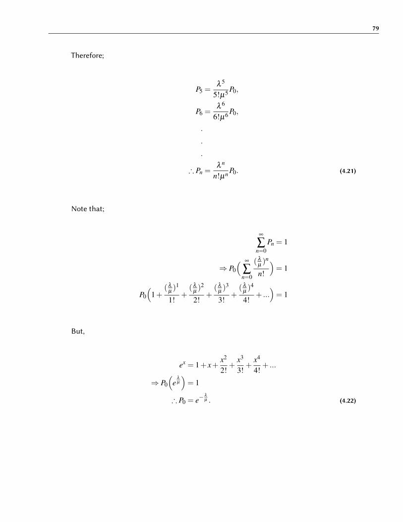
79

Therefore;

P5 =λ 5

5!µ5 P0,

P6 =λ 6

6!µ6 P0,

.

.

.

∴ Pn =λ n

n!µn P0. (4.21)

Note that;

∞

∑n=0

Pn = 1

⇒ P0

( ∞

∑n=0

(λ

µ)n

n!

)= 1

P0

(1+

(λ

µ)1

1!+

(λ

µ)2

2!+

(λ

µ)3

3!+

(λ

µ)4

4!+ ...

)= 1

But,

ex = 1+ x+x2

2!+

x3

3!+

x4

4!+ ...

⇒ P0

(e

λ

µ

)= 1

∴ P0 = e−λ

µ . (4.22)

80

Therefore,

P1 =(λ

µ)1

1!e−

λ

µ ,

P2 =(λ

µ)2

2!e−

λ

µ ,

P3 =(λ

µ)3

3!e−

λ

µ ,

P4 =(λ

µ)4

4!e−

λ

µ ,

.

.

.


Pn =(λ

µ)n

n!P0.

Hence, Pn =(λ

µ)n

n!e−

λ

µ , n = 0,1,2,3, ...

Thus, the limiting distribution is a Poisson distribution with parameter λ

µ. It is independent

of the initial state.Using Proposition (2.1)We have;


µ1µ2µ3...µnP0

But, λ0 = λ1 = λ2 = λ3 = ...= λn−1 = λ ,

and

µ1 = µ, µ2 = 2µ, µ3 = 3µ, ..., µn = nµ.


µ2µ3µ...nµP0

∴ Pn =λ n

n!µn P0

81


P0 = e−λ

µ

∴ Pn =λ n

n!µn e−λ

µ .


µ.


Pn

Pn−1=

λn−1

µn, µn 6= 0

But, λn−1 = λ ,

and

µn = nµ.

∴Pn

Pn−1=

λ

nµ.

⇒ nµPn = λPn−1 (4.23)


∞

∑n=0

nµPnsn =∞

∑n=0

λPn−1sn

µs∞

∑n=0

nPnsn−1 = λ s∞

∑n=0

Pn−1sn−1

sµdψ(s)

ds= sλψ(s)

dψ(s)ψ(s)

=λ

µds

82


∫ dψ(s)ψ(s)

=∫

λ

µds

lnψ(s) =λ

µs+ c

ψ(s) = c1eλ

µs

Pu�ing s=1;

ψ(1) = 1 = c1eλ

µ

⇒ c1 = e−λ

µ .

∴ ψ(s) = e−λ

µ eλ

µs

∴ ψ(s) = e−λ

µ(1−s).


µ.

ψ′(s) =

λ

µe−

λ

µ(1−s)

ψ′′(s) = (

λ

µ)2e−

λ

µ(1−s)

E(X) = ψ′(1)

∴ E(X) =λ

µ.

Var(x) = ψ′′(1)+ψ

′(1)− [ψ

′(1)]2

= (λ

µ)2 +

λ

µ− [

λ

µ]2

∴Var(X) =λ

µ.

83


1F1(ε;ε;λ

µ) = 1+

ε

ε

λ

µ

1!+

ε(ε +1)ε(ε +1)

(λ

µ)2

2!+ ...+

(ε +n−1)(ε +n−1)

(λ

µ)n

n!

=∞

∑n=0

ε(ε +1)(ε +2)...(ε +n−1)ε(ε +1)(ε +2)...(ε +n−1)

(λ

µ)n

n!

=∞

∑n=0

(ε +n−1)(ε +n−2)...(ε +2)(ε +1)ε(ε +n−1)(ε +n−2)...(ε +2)(ε +1)ε

Γ(ε)

Γ(ε).Γ(ε)

Γ(ε).(λ

µ)n

n!

=∞

∑n=0

Γ(ε +n)Γ(ε +n)

Γ(ε)

Γ(ε).(λ

µ)n

n!


1 =∞

∑n=0

Γ(ε +n)Γ(ε +n)

Γ(ε)

Γ(ε).

1

1F1(ε;ε; λ

µ)

(λ

µ)n

n!

Therefore,

Pn = Prob.(N = n)

=Γ(ε +n)Γ(ε +n)

Γ(ε)

Γ(ε).

1

1F1(ε;ε; λ

µ)

(λ

µ)n

n!


φ(z) =∞

∑n=0

Pnzn

=Γ(ε +n)Γ(ε +n)

Γ(ε)

Γ(ε)

(λ

µz)n

n!.

1

1F1(ε;ε; λ

µ)

∴ φ(z) =1F1(ε;ε; λ

µz)

1F1(ε;ε; λ

µ).

84

Therefore,

φ′(z) =

λ

µ

1F1(ε +1;ε +1; λ

µz)

1F1(ε;ε; λ

µ)

φ′′(z) = (

λ

µ)2 1F1(ε +2;ε +2; λ

µz)

1F1(ε;ε; λ

µ)

Let, Λκ =1F1(ε +κ;ε +κ; λ

µ)

1F1(ε;ε; λ

µ)

; κ = 1,2.

∴ E(x) =λ

µΛ1.

Var(X) = φ′′(1)+φ

′(1)− [φ

′(1)]2

= (λ

µ)2

Λ2 +λ

µΛ1− (

λ

µ)2

Λ21

∴Var(X) =λ

µΛ1 +(

λ

µ)2(Λ2−Λ

21).

4.4 M|M|S|GD|∞ �euing Process

An M|M|S|GD|∞ �euing Process uses Poisson arrivals and exponential service time dis-tribution with s parallel servers.The queue discipline is general and the number of customers in the system and the size oftheir source or where the customers come from are infinite.In this case,

λn = λ , for n = 0,1,2,3, ...

µn = min(n,s) for n = 1,2,3, ...

⇒ µn = nµ, (n < s)

µn = sµ, (n≥ s).

85

The basic di�erence di�erential equations for the steady state are:

0 = µP1−λP0 (4.24)

0 = (n+1)µPn+1 +λPn−1− (λ +nµ)Pn, for n < s (4.25)

0 = sµPn+1 +λPn−1− (λ + sµ)Pn, for n≥ s (4.26)


Pn =λ n

n!µn e−λ

µ , for n < s


λP0 = µP1

⇒ λ

µP0 = P1

∴ P1 =λ

µP0. (4.27)


0 = 2µP2 +λP0− (λ +µ)P1 (4.28)

86


0 = 2µP2 +λP0− (λ +µ)λ

µP0

0 = 2µP2 +λP0−λP0−λ 2

µP0

0 = 2µP2−λ 2

µP0

⇐⇒ λ 2

µP0 = 2µP2

⇒ λ 2

2!µ2 P0 = P2

∴ P2 =λ 2

2!µ2 P0. (4.29)


0 = 3µP3 +λP1− (λ +2µ)P2 (4.30)


0 = 3µP3 +λ 2

µP0− (λ +2µ)

λ 2

2!µ2 P0

0 = 3µP3 +λ 2

µP0−

λ 2

µP0−

λ 3

2!µ2 P0

0 = 3µP3−λ 3

2!µ2 P0

⇐⇒ λ 3

2!µ2 P0 = 3µP3

⇒ λ 3

3!µ3 P0 = P3

∴ P3 =λ 3

3!µ3 P0.

87

Thus,

P4 =λ 4

4!µ4 P0,

P5 =λ 5

5!µ5 P0,

.

.

.

Pn =λ n

n!µn P0. (4.31)

Let,

∞

∑n=0

Pn = 1

P0

( ∞

∑n=0

λ n

n!µn

)= 1

P0

(1+

λ 1

1!µ1 +λ 2

2!µ2 +λ 3

3!µ3 +λ 4

4!µ4 + ...)= 1

P0

(e

λ

µ

)= 1

∴ P0 = e−λ

µ . (4.32)

From (4.31) and (4.32) above, we have;

Pn =λ n

n!µn P0.

∴ Pn =λ n

n!µn e−λ

µ . for n < s


µ.

Using Proposition (2.1)We have that;

88


µ1µ2µ3...µnP0

But, λ0 = λ1 = λ2 = λ3 = ...= λn−1 = λ ,

and

µ1 = µ, µ2 = 2µ, µ3 = 3µ, ..., µn = nµ.


µ2µ3µ...nµP0

=λ n

n!µn P0


P0 = e−λ

µ

∴ Pn =λ n

n!µn e−λ

µ .


µ.


Pn

Pn−1=

λn−1

µn, µn 6= 0

But, λn−1 = λ ,

and

µn = nµ.

∴Pn

Pn−1=

λ

nµ.

⇒ nµPn = λPn−1 (4.33)

89


∞

∑n=0

nµPnsn =∞

∑n=0

λPn−1sn

µs∞

∑n=0

nPnsn−1 = λ s∞

∑n=0

Pn−1sn−1

sµdψ(s)

ds= sλψ(s)

dψ(s)ψ(s)

=λ

µds


∫ dψ(s)ψ(s)

=∫

λ

µds

lnψ(s) =λ

µs+ c

ψ(s) = c1eλ

µs

Pu�ing s=1;

ψ(1) = 1 = c1eλ

µ

⇒ c1 = e−λ

µ .

∴ ψ(s) = e−λ

µ eλ

µs

∴ ψ(s) = e−λ

µ(1−s).

90


µ.

ψ′(s) =

λ

µe−

λ

µ(1−s)

ψ′′(s) = (

λ

µ)2e−

λ

µ(1−s)

E(X) = ψ′(1)

∴ E(X) =λ

µ.

Var(x) = ψ′′(1)+ψ

′(1)− [ψ

′(1)]2

= (λ

µ)2 +

λ

µ− [

λ

µ]2

∴Var(X) =λ

µ.


1F1(ω;ω;λ

µ) = 1+

ω

ω

λ

µ

1!+

ω(ω +1)ω(ω +1)

(λ

µ)2

2!+ ...+

(ω +n−1)(ω +n−1)

(λ

µ)n

n!

=∞

∑n=0

ω(ω +1)(ω +2)...(ω +n−1)ω(ω +1)(ω +2)...(ω +n−1)

(λ

µ)n

n!

=∞

∑n=0

(ω +n−1)(ω +n−2)...(ω +2)(ω +1)ω(ω +n−1)(ω +n−2)...(ω +2)(ω +1)ω

Γ(ω)

Γ(ω).Γ(ω)

Γ(ω).(λ

µ)n

n!

=∞

∑n=0

Γ(ω +n)Γ(ω +n)

Γ(ω)

Γ(ω).(λ

µ)n

n!


1 =∞

∑n=0

Γ(ω +n)Γ(ω +n)

Γ(ω)

Γ(ω).

1

1F1(ω;ω; λ

µ)

(λ

µ)n

n!

Therefore,

Pn = Prob.(N = n)

=Γ(ω +n)Γ(ω +n)

Γ(ω)

Γ(ω).

1

1F1(ω;ω; λ

µ)

(λ

µ)n

n!

91


φ(z) =∞

∑n=0

Pnzn

=Γ(ω +n)Γ(ω +n)

Γ(ω)

Γ(ω)

(λ

µz)n

n!.

1

1F1(ω;ω; λ

µ)

∴ φ(z) =1F1(ω;ω; λ

µz)

1F1(ω;ω; λ

µ).

φ′(z) =

λ

µ

1F1(ω +1;ω +1; λ

µz)

1F1(ω;ω; λ

µ)

φ′′(z) = (

λ

µ)2 1F1(ω +2;ω +2; λ

µz)

1F1(ω;ω; λ

µ)

Let, Λκ =1F1(ω +κ;ω +κ; λ

µ)

1F1(ω;ω; λ

µ)

; κ = 1,2.

∴ E(x) =λ

µΛ1.

Var(X) = φ′′(1)+φ

′(1)− [φ

′(1)]2

= (λ

µ)2

Λ2 +λ

µΛ1− (

λ

µ)2

Λ21

∴Var(X) =λ

µΛ1 +(

λ

µ)2(Λ2−Λ

21).


0 = sµP2 +λP0− (λ + sµ)P1 (4.34)

92


0 = sµP2 +λP0− (λ + sµ)λ

µP0

0 = sµP2 +λP0− sλP0−λ 2

µP0

0 = sµP2−λ (s−1)P0−λ 2

µP0

⇐⇒ λ 2

µP0 +λ (s−1)P0 = sµP2

⇒ 1s

(λ 2

µ2 +λ

µ(s−1)

)P0 = P2

∴ P2 =1s

(λ 2

µ2 +λ

µ(s−1)

)P0. (4.35)


0 = sµP3 +λP1− (λ + sµ)P2 (4.36)


0 = sµP3 +λ 2

µP0− (λ + sµ)

1s

(λ 2

µ2 +λ

µ(s−1)

)P0

0 = sµP3 +λ 2

µP0−λ (s−1)P0−

λ 2

µP0−

λ 2

sµ(s−1)P0−

λ 3

sµ2 P0

0 = sµP3−λ (s−1)P0−λ 2

sµ(s−1)P0−

λ 3

sµ2 P0

⇐⇒ λ (s−1)P0 +λ 2

sµ(s−1)P0 +

λ 3

sµ2 P0 = sµP3

⇒ 1s2

(λ

µs(s−1)+

λ 2

µ2 (s−1)+λ 3

µ3

)P0 = P3

∴ P3 =1s2

(λ 3

µ3 +λ 2

µ2 (s−1)+λ

µs(s−1)

)P0.

93

Thus,

P4 =1s3

(λ 4

µ4 +λ 3

µ3 (s−1)+λ 2

µ2 s(s−1)+λ

µs(s−1)(s−2)

)P0,

.

.

.

Pn =1

sn−s

(λ n

µn +λ n−1

µn−1 (s−1)+ ...+λ

µs(s−1)(s−2)...(s−n)

)P0. for n≥ s

Assume that λ

µ< s, we have;

Then,

∞

∑n=0

Pn = 1

P0

( ∞

∑n=0

λ n

n!µn

)= 1

P0

(1+

λ 1

1!µ1 +λ 2

2!µ2 +λ 3

3!µ3 +λ 4

4!µ4 + ...)= 1

P0

(e

λ

µ

)= 1

∴ P0 = e−λ

µ .

We find that;

Pn =(λ

µ)n

s!sn−s e−λ

µ . for n≥ s (λ

µ< s)

Remark 4.2(1) If the series ∑(Pn

P0) converges only in λ

µ< s. i.e., ∑Pn = 1.

(2) If λ

µ≥ s, a limiting distribution Pn cannot exists. In this case Pn = 0 for all n, which

means that gradually the waiting line grows over all bounds.

94

4.5 M|M|1|GD|c|∞ �eueing System

The M|M|1|GD|c|∞ queuing process uses a Poisson arrivals or exponential intervals ex-ponential service time distribution with one server, the queueing discipline is general, ccustomers are allowed in the system (in queue plus in service) and the size of the sourcefrom where the customers arrive is finite.In this case, the system can accomodate only c units so that a unit/customer which arriveswhen the system is in state Ec is not allowed into the system.System is said to be in state En if there are exactly n units/persons either being served orin the waiting line, (n≤ c−1).Here,

λn = λ , for n = 0,1,2,3, ...,c−1

and

µn = nµ, for n≤ c−1

µn = µ, for n = 1,2,3, ...,c.

For the steady state problem, t→ ∞ implying that Pn(t) is independent of t.Thus,

Pn(t) = Pn,

and

limt→∞

P′n(t) = 0.

Hence the basic di�erence di�erential equations for the steady state, at state En(n ≤c−1), are:

0 = µP1−λP0, for n = 0 (4.37)

0 = (n+1)µPn+1 +λPn−1− (λ +nµ)Pn; for n≤ c−1. (4.38)


Pn = e−λ

µ

(λ

µ)n

n!(4.39)

95


λP0 = µP1

⇒ λ

µP0 = P1

∴ P1 =λ

µP0. (4.40)

Solving steady state equation iteratively, we have;When n=1;Equation (4.38) becomes;

0 = 2µP2 +λP0− (λ +µ)P1 (4.41)


0 = 2µP2 +λP0− (λ +µ)λ

µP0

0 = 2µP2 +λP0−λP0−λ 2

µP0

0 = 2µP2−λ 2

µP0

⇐⇒ λ 2

µP0 = 2µP2

⇒ λ 2

2!µ2 P0 = P2

∴ P2 =λ 2

2!µ2 P0. (4.42)


0 = 3µP3 +λP1− (λ +2µ)P2 (4.43)

96


0 = 3µP3 +λ 2

µP0− (λ +2µ)

λ 2

2!µ2 P0

0 = 3µP3 +λ 2

µP0−

λ 2

µP0−

λ 3

2!µ2 P0

0 = 3µP3−λ 3

2!µ2 P0

⇐⇒ λ 3

2!µ2 P0 = 3µP3

⇒ λ 3

3!µ3 P0 = P3

∴ P3 =λ 3

3!µ3 P0.

Thus,

P4 =λ 4

4!µ4 P0,

P5 =λ 5

5!µ5 P0,

.

.

.

Pn =(λ

µ)n

n!P0. (4.44)

Let,

c−1

∑n=0

Pn = 1

As c−1→ ∞.

Then,

97

P0 +P1 +P2 +P3 + ...+Pc−1 = 1

P0

(1+

(λ

µ)1

1!+

(λ

µ)2

2!+

(λ

µ)3

3!+ ...

)= 1

P0

(e

λ

µ

)= 1

∴ P0 = e−λ

µ . (4.45)

Hence, from (4.44) and (4.45), we have;

Pn =(λ

µ)n

n!P0

∴ Pn =(λ

µ)n

n!e−

λ

µ .


µ. It is independent of the

initial condition.Using Proposition (2.1)We have that;


µ1µ2µ3...µnP0

But, λ0 = λ1 = λ2 = λ3 = ...= λn−1 = λ ,

and

µ1 = µ, µ2 = 2µ, µ3 = 3µ, ..., µn = nµ.


µ2µ3µ...nµP0

∴ Pn =(λ

µ)n

n!P0


P0 = e−λ

µ

∴ Pn ==(λ

µ)n

n!e−

λ

µ .

98


µ.


Pn

Pn−1=

λn−1

µn, µn 6= 0

But, λn−1 = λ ,

and

µn = nµ.

∴Pn

Pn−1=

λ

nµ.

⇒ nµPn = λPn−1 (4.46)


∞

∑n=0

nµPnsn =∞

∑n=0

λPn−1sn

µs∞

∑n=0

nPnsn−1 = λ s∞

∑n=0

Pn−1sn−1

sµdψ(s)

ds= sλψ(s)

dψ(s)ψ(s)

=λ

µds


∫ dψ(s)ψ(s)

=∫

λ

µds

lnψ(s) =λ

µs+ c

ψ(s) = c1eλ

µs

99

Pu�ing s=1;

ψ(1) = 1 = c1eλ

µ

⇒ c1 = e−λ

µ .

∴ ψ(s) = e−λ

µ eλ

µs

∴ ψ(s) = e−λ

µ(1−s).


µ.

ψ′(s) =

λ

µe−

λ

µ(1−s)

ψ′′(s) = (

λ

µ)2e−

λ

µ(1−s)

E(X) = ψ′(1)

∴ E(X) =λ

µ.

Var(x) = ψ′′(1)+ψ

′(1)− [ψ

′(1)]2

= (λ

µ)2 +

λ

µ− [

λ

µ]2

∴Var(X) =λ

µ.


1F1(υ ;υ ;λ

µ) = 1+

υ

υ

λ

µ

1!+

υ(υ +1)υ(υ +1)

(λ

µ)2

2!+ ...+

(υ +n−1)(υ +n−1)

(λ

µ)n

n!

=∞

∑n=0

υ(υ +1)(υ +2)...(υ +n−1)υ(υ +1)(υ +2)...(υ +n−1)

(λ

µ)n

n!

=∞

∑n=0

(υ +n−1)(υ +n−2)...(υ +2)(υ +1)υ(υ +n−1)(υ +n−2)...(υ +2)(υ +1)υ

Γ(υ)

Γ(υ).Γ(υ)

Γ(υ).(λ

µ)n

n!

=∞

∑n=0

Γ(υ +n)Γ(υ +n)

Γ(υ)

Γ(υ).(λ

µ)n

n!

100


1 =∞

∑n=0

Γ(υ +n)Γ(υ +n)

Γ(υ)

Γ(υ).

1

1F1(υ ;υ ; λ

µ)

(λ

µ)n

n!

Therefore,

Pn = Prob.(N = n)

=Γ(υ +n)Γ(υ +n)

Γ(υ)

Γ(υ).

1

1F1(υ ;υ ; λ

µ)

(λ

µ)n

n!


φ(z) =∞

∑n=0

Pnzn

=Γ(υ +n)Γ(υ +n)

Γ(υ)

Γ(υ)

(λ

µz)n

n!.

1

1F1(υ ;υ ; λ

µ)

∴ φ(z) =1F1(υ ;υ ; λ

µz)

1F1(υ ;υ ; λ

µ).

φ′(z) =

λ

µ

1F1(υ +1;υ +1; λ

µz)

1F1(υ ;υ ; λ

µ)

φ′′(z) = (

λ

µ)2 1F1(υ +2;υ +2; λ

µz)

1F1(υ ;υ ; λ

µ)

Let, Λκ =1F1(υ +κ;υ +κ; λ

µ)

1F1(υ ;υ ; λ

µ)

; κ = 1,2.

∴ E(x) =λ

µΛ1.

Var(X) = φ′′(1)+φ

′(1)− [φ

′(1)]2

= (λ

µ)2

Λ2 +λ

µΛ1− (

λ

µ)2

Λ21

∴Var(X) =λ

µΛ1 +(

λ

µ)2(Λ2−Λ

21).

101

4.6 M|M|1|§ �euing Preocess

In this queueing process, the assumption is that the system accommodates finite § numberof units, the one being served included if any. Here, customers uses a Poisson arrivalsprocess with a rate λ say; the customer only join the system when there are less than§ units/customers and when a customer arrives and find § in the system will leave thesystem and be lost. The service time is exponential with µ rate.When the system is at state E§ or when there are § customers in the system, it meansthat no more customers allowed in the system and hence the number of customers cannotexceed § in the system. This implies that when the system is at state §, departures only ispossible.Thus, this implies that;

λn = µn

⇒ λ = µ.

Therfore, the basic di�erence di�erential equations for the steady state are:

0 = µP1−λP0, (4.47)

and

0 = µPn+1−λPn, for n = 0,1,2,3, ...,§−1. (4.48)


Pn =(

λ

µ

)n(1− λ

µ

). (4.49)


λP0 = µP1

⇒ λ

µP0 = P1

∴ P1 =λ

µP0. (4.50)

102

Solving steady state equations iteratively, we have;When n=1;Equation (4.48) becomes;

0 = µP2−λP1 (4.51)


0 = µP2−λ 2

µP0

⇐⇒ λ 2

µP0 = µP2

⇒ λ 2

µ2 P0 = P2

∴ P2 =λ 2

µ2 P0. (4.52)


0 = µP3−λP2 (4.53)


0 = µP3−λ 3

µ2 P0

⇐⇒ λ 3

µ2 P0 = µP3

⇒ λ 3

µ3 P0 = P3

∴ P3 =λ 3

µ3 P0.

103

Thus,

P4 =λ 4

µ4 P0,

P5 =λ 5

µ5 P0,

.

.

.

Pn = (λ

µ)nP0. (4.54)

When applying the normalizing conditions, we have;

§

∑n=0

Pn = 1

P0

( §

∑n=0

(λ

µ)n)= 1

P0

(1+(

λ

µ)1 +(

λ

µ)2 +(

λ

µ)3 +(

λ

µ)4 + ...

)= 1

Note that;

11− x

= 1+ x+ x2 + x3 + x4 + ...

∴ P0

( 1

1− λ

µ

)= 1

∴ P0 = 1− λ

µ. (4.55)

⇒ P1 =(

λ

µ

)1(1− λ

µ

),

P2 =(

λ

µ

)2(1− λ

µ

),

104

Therefore,

P3 =(

λ

µ

)3(1− λ

µ

),

P4 =(

λ

µ

)4(1− λ

µ

),

.

.

.


Pn =(

λ

µ

)n(1− λ

µ

). for n = 0,1,2,3, ...,§−1. (4.56)

When n=0,1,2,3,4, . . . ,§ we have that;

Pn =(1− λ

µ)(λ

µ)n

1− (λ

µ)§+1

; λ 6= µ.

and (4.57)

Pn =1

§+1; λ = µ.

Therefore, the limiting distribution is Uniform distribution when λ

µ= 1 and truncated

Geometric distribution when λ

µ6= 1.



µ1µ2µ3...µnP0

But, λ0 = λ1 = λ2 = λ3 = ...= λn−1 = λ ,

and

µ1 = µ, µ2 = µ, µ3 = µ, ..., µn = µ.

105


µµµ...µP0

∴ Pn =(

λ

µ

)nP0


P0 =(

1− λ

µ

).

∴ Pn =(

λ

µ

)n(1− λ

µ

), for n = 0,1,2,3, ...,§−1.

Which is a Geometric distribution with parameter λ

µ.


Pn

Pn−1=

λn−1

µn, µn 6= 0

But, λn−1 = λ ,

and

µn = µ.

∴Pn

Pn−1=

λ

µ.

⇒ µPn = λPn−1 (4.58)


∞

∑n=0

µPnsn =∞

∑n=0

λPn−1sn

µ

∞

∑n=0

Pnsn = λ s∞

∑n=0

Pn−1sn−1

(1− λ

µs)ψ(s) = P0

But, P0 = 1− λ

µ.

∴ ψ(s) =(1− λ

µ)

(1− λ

µs).

106

Which is a Geometric distribution with parameter λ

µ.

ψ′(s) =

λ

µ(1− λ

µ)

(1− λ

µs)2

ψ′′(s) =

2(λ

µ)2(1− λ

µ)

(1− λ

µs)3

E(X) = ψ′(1)

=

λ

µ(1− λ

µ)

(1− λ

µ)2

∴ E(X) =

λ

µ

(1− λ

µ).

Var(x) = ψ′′(1)+ψ

′(1)− [ψ

′(1)]2

=2(λ

µ)2(1− λ

µ)

(1− λ

µ)3

+

λ

µ(1− λ

µ)

(1− λ

µ)2− [

λ

µ(1− λ

µ)

(1− λ

µs)2

]2

=2(λ

µ)2

(1− λ

µ)2

+

λ

µ

(1− λ

µ)−

(λ

µ)2

(1− λ

µs)2

=(λ

µ)2

(1− λ

µ)2

+

λ

µ

(1− λ

µ)

∴Var(X) =(λ

µ)2 + λ

µ(1− λ

µ)

(1− λ

µ)2

∴Var(X) =

λ

µ

(1− λ

µ)2.

107

From Kummer’s confluent hypergeometric series, we have that;

1F1(ι ; ι ;λ

µ) = 1+

ι

ι

λ

µ

1!+

ι(ι +1)ι(ι +1)

(λ

µ)2

2!+ ...+

(ι +n−1)(ι +n−1)

(λ

µ)n

n!

=∞

∑n=0

ι(ι +1)(ι +2)...(ι +n−1)ι(ι +1)(ι +2)...(ι +n−1)

(λ

µ)n

n!

=∞

∑n=0

(ι +n−1)(ι +n−2)...(ι +2)(ι +1)ι(ι +n−1)(ι +n−2)...(ι +2)(ι +1)ι

Γ(ρ)

Γ(ι).Γ(ι)

Γ(ι).(λ

µ)n

n!

=∞

∑n=0

Γ(ι +n)Γ(ι +n)

Γ(ι)

Γ(ι).(λ

µ)n

n!


1 =∞

∑n=0

Γ(ι +n)Γ(ι +n)

Γ(ι)

Γ(ι).

1

1F1(ι ; ι ; λ

µ)

(λ

µ)n

n!

Therefore,

Pn = Prob.(N = n)

=Γ(ι +n)Γ(ι +n)

Γ(ι)

Γ(ι).

1

1F1(ι ; ι ; λ

µ)

(λ

µ)n

n!


φ(z) =∞

∑n=0

Pnzn

=Γ(ι +n)Γ(ι +n)

Γ(ι)

Γ(ι)

(λ

µz)n

n!.

1

1F1(ι ; ι ; λ

µ)

∴ φ(z) =1F1(ι ; ι ; λ

µz)

1F1(ι ; ι ; λ

µ).

φ′(z) =

λ

µ

1F1(ι +1; ι +1; λ

µz)

1F1(ι ; ι ; λ

µ)

108

Therefore,

φ′′(z) = (

λ

µ)2 1F1(ι +2; ι +2; λ

µz)

1F1(ι ; ι ; λ

µ)

Let, Λκ =1F1(ι +κ; ι +κ; λ

µ)

1F1(ι ; ι ; λ

µ)

; κ = 1,2.

∴ E(x) =λ

µΛ1.

Var(X) = φ′′(1)+φ

′(1)− [φ

′(1)]2

= (λ

µ)2

Λ2 +λ

µΛ1− (

λ

µ)2

Λ21

∴Var(X) =λ

µΛ1 +(

λ

µ)2(Λ2−Λ

21).

4.7 M|M|c|c �eueing Process

Suppose we consider a c-server model with Poisson input and exponential service timesuch that when all the c-channels are busy, a customer leaves the system without waitingfor service.In this case:

λn = λ ; for n = 0,1,2,3, ...,c−1

and

µn = nµ; for n = 0,1,2,3, ...,c−1

µn = cµ; for n≥ c.

The basic di�erence di�erential equations for the steady state are:

0 = µP1−λP0 (4.59)

0 = (n+1)µPn+1 +λPn−1− (λ +nµ)Pn; for n = 0,1,2, ...,c−1 (4.60)

0 = cµPn+1 +λPn−1− (λ + cµ)Pn; for n = c+1,c+2, ... (4.61)


109

Pn =(λ

µ)n

n!e−

λ

µ , for n = 0,1,2, ...,c−1.

Pn =(λ

µ)n

c!cn−c e−λ

µ . for n≥ c (λ

µ< c)

ProofSolving steady state equations iteratively, we have;Equation (4.59) can be expressed as;

λP0 = µP1

⇒ λ

1µP0 = P1

∴ P1 =(λ

µ)1

1!P0. (4.62)


0 = 2µP2 +λP0− (λ +µ)P1 (4.63)


0 = 2µP2 +λP0− (λ +µ)λ

µP0

0 = 2µP2 +λP0−λP0−λ 2

µP0

0 = 2µP2−λ 2

µP0

⇐⇒ λ 2

µP0 = 2µP2

⇒ λ 2

2.1µ2 P0 = P2

∴ P2 =(λ

µ)2

2!P0. (4.64)

110


0 = 3µP3 +λP1− (λ +2µ)P2 (4.65)


0 = 3µP3 +λ 2

µP0− (λ +2µ)

λ 2

2!µ2 P0

0 = 3µP3 +λ 2

µP0−

λ 2

µP0−

λ 3

2.1µ2 P0

0 = 3µP3−λ 3

2.1µ2 P0

⇐⇒ λ 3

2.1µ2 P0 = 3µP3

⇒ λ 3

3.2.1µ3 P0 = 3P3

∴ P3 =(λ

µ)3

3!P0.

Thus,

P4 =(λ

µ)4

4!P0,

P5 =(λ

µ)5

5!P0,

.

.

.

Pn =(λ

µ)n

n!P0, for n = 0,1,2,3, ...,c−1. (4.66)

Suppose that c−1→ ∞.

Then,

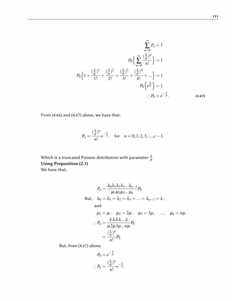
111

∞

∑n=0

Pn = 1

P0

{ ∞

∑n=0

(λ

µ)n

n!

}= 1

P0

{1+

(λ

µ)1

1!+

(λ

µ)2

2!+

(λ

µ)3

3!+

(λ

µ)4

4!+ ...

}= 1

P0

{e

λ

µ

}= 1

∴ P0 = e−λ

µ . (4.67)

From (4.66) and (4.67) above, we have that;

Pn =(λ

µ)n

n!e−

λ

µ . for n = 0,1,2,3, ...,c−1.

Which is a truncated Poisson distribution with parameter λ

µ.



µ1µ2µ3...µnP0

But, λ0 = λ1 = λ2 = λ3 = ...= λn−1 = λ ,

and

µ1 = µ, µ2 = 2µ, µ3 = 3µ, ..., µn = nµ.


µ2µ3µ...nµP0

=(λ

µ)n

n!P0


P0 = e−λ

µ

∴ Pn =(λ

µ)n

n!e−

λ

µ .

112


µ.


Pn

Pn−1=

λn−1

µn, µn 6= 0

But, λn−1 = λ ,

and

µn = nµ.

∴Pn

Pn−1=

λ

nµ.

Pn

Pn−1=

λ

nµ

⇒ nµPn = λPn−1 (4.68)


∞

∑n=0

nµPnsn =∞

∑n=0

λPn−1sn

µs∞

∑n=0

nPnsn−1 = λ s∞

∑n=0

Pn−1sn−1

sµdψ(s)

ds= sλψ(s)

dψ(s)ψ(s)

=λ

µds


∫ dψ(s)ψ(s)

=∫

λ

µds

lnψ(s) =λ

µs+ c

ψ(s) = c1eλ

µs

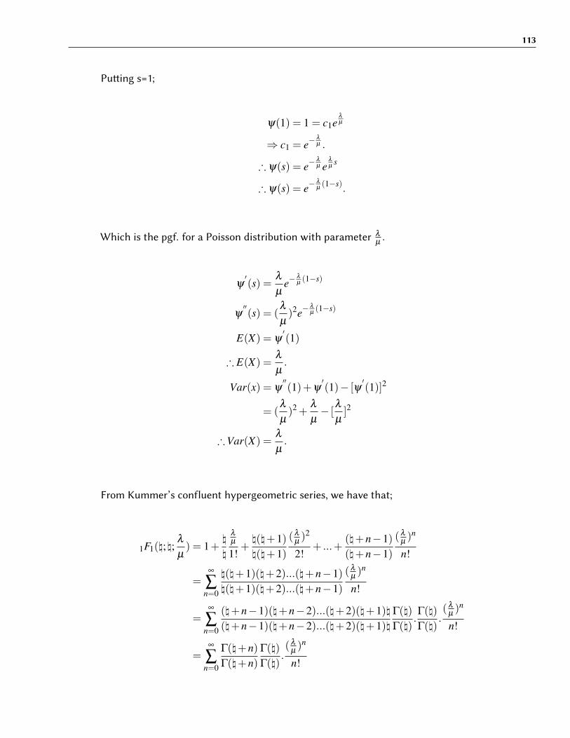
113

Pu�ing s=1;

ψ(1) = 1 = c1eλ

µ

⇒ c1 = e−λ

µ .

∴ ψ(s) = e−λ

µ eλ

µs

∴ ψ(s) = e−λ

µ(1−s).


µ.

ψ′(s) =

λ

µe−

λ

µ(1−s)

ψ′′(s) = (

λ

µ)2e−

λ

µ(1−s)

E(X) = ψ′(1)

∴ E(X) =λ

µ.

Var(x) = ψ′′(1)+ψ

′(1)− [ψ

′(1)]2

= (λ

µ)2 +

λ

µ− [

λ

µ]2

∴Var(X) =λ

µ.

From Kummer’s confluent hypergeometric series, we have that;

1F1(\;\;λ

µ) = 1+

\

\

λ

µ

1!+

\(\+1)\(\+1)

(λ

µ)2

2!+ ...+

(\+n−1)(\+n−1)

(λ

µ)n

n!

=∞

∑n=0

\(\+1)(\+2)...(\+n−1)\(\+1)(\+2)...(\+n−1)

(λ

µ)n

n!

=∞

∑n=0

(\+n−1)(\+n−2)...(\+2)(\+1)\(\+n−1)(\+n−2)...(\+2)(\+1)\

Γ(\)

Γ(\).Γ(\)

Γ(\).(λ

µ)n

n!

=∞

∑n=0

Γ(\+n)Γ(\+n)

Γ(\)

Γ(\).(λ

µ)n

n!

114


1 =∞

∑n=0

Γ(\+n)Γ(\+n)

Γ(\)

Γ(\).

1

1F1(\;\; λ

µ)

(λ

µ)n

n!

Therefore,

Pn = Prob.(N = n)

=Γ(\+n)Γ(\+n)

Γ(\)

Γ(\).

1

1F1(\;\; λ

µ)

(λ

µ)n

n!


φ(z) =∞

∑n=0

Pnzn

=Γ(\+n)Γ(\+n)

Γ(\)

Γ(\)

(λ

µz)n

n!.

1

1F1(\;\; λ

µ)

∴ φ(z) =1F1(\;\; λ

µz)

1F1(\;\; λ

µ).

φ′(z) =

λ

µ

1F1(\+1;\+1; λ

µz)

1F1(\;\; λ

µ)

φ′′(z) = (

λ

µ)2 1F1(\+2;\+2; λ

µz)

1F1(\;\; λ

µ)

Let, Λκ =1F1(\+κ;\+κ; λ

µ)

1F1(\;\; λ

µ)

; κ = 1,2.

∴ E(x) =λ

µΛ1.

Var(X) = φ′′(1)+φ

′(1)− [φ

′(1)]2

= (λ

µ)2

Λ2 +λ

µΛ1− (

λ

µ)2

Λ21

∴Var(X) =λ

µΛ1 +(

λ

µ)2(Λ2−Λ

21).


115

0 = cµP2 +λP0− (λ + cµ)P1 (4.69)


0 = cµP2 +λP0− (λ + cµ)λ

µP0

0 = cµP2 +λP0− cλP0−λ 2

µP0

0 = cµP2−λ (c−1)P0−λ 2

µP0

⇐⇒ λ 2

µP0 +λ (c−1)P0 = cµP2

⇒ 1c

(λ 2

µ2 +λ

µ(c−1)

)P0 = P2

∴ P2 =1c

(λ 2

µ2 +λ

µ(c−1)

)P0. (4.70)


0 = cµP3 +λP1− (λ + cµ)P2 (4.71)


0 = cµP3 +λ 2

µP0− (λ + cµ)

1c

(λ 2

µ2 +λ

µ(c−1)

)P0

0 =− λ 3

cµ2 P0−λ 2

cµ(c−1)P0−

λ 2

µP0−λ (c−1)P0 +

λ 2

µP0 + cµP3

0 =− λ 3

cµ2 P0−λ 2

cµ(c−1)P0−λ (c−1)P0 + cµP3

116

Therefore,

⇐⇒ cµP3 =1c

(λ 3

µ2 +λ 2

µ(c−1)+λc(c−1)

)P0

⇒ P3 =1c2

(λ 3

µ3 +λ 2

µ2 (c−1)+λ

µc(c−1)

)P0

∴ P3 =1c2

(λ 3

µ3 +λ 2

µ2 (c−1)+λ

µc(c−1)

)P0.

Therefore,

P4 =1c3

(λ 4

µ4 +λ 3

µ3 (c−1)+λ 2

µ2 c(c−1)+λ

µc(c−1)(c−2)

)P0,

.

.

.

Pn =1

cn−c

(λ n

µn +λ n−1

µn−1 (c−1)+λ n−2

µn−2 c(c−1)+ ...+λ

µc(c−1)...(c−n)

)P0, for n≥ c.

Supposed that λ

µ< c,

Then,

∑Pn = 1

⇒ P0 +P1 +P2 +P3 + ...+Pn = 1

1cn−c P0

{1+

(λ

µ)1

1!+

(λ

µ)2

2!+

(λ

µ)3

3!+

(λ

µ)4

4!+ ...

}= 1

P0

(e

λ

µ

)= 1

∴ P0 = e−λ

µ .

∴ Pn =(λ

µ)n

c!cn−c e−λ

µ . for n≥ c (λ

µ< c)

117

Note that;

Pn =

( λ

µ)n

n!

∑c§=0

( λ

µ)§

§!

, for n = 0,1,2, ...,c.

Which is the Erlang’s distribution/formula.Suppose that the unit that arrived in the system is lost because upon arrival, it found thatall the channels in the system are busy.Then, the probability of this event will be given by;

Pc =

( λ

µ)c

c!

∑c§=0

( λ

µ)§

§!

. (4.72)

Equation (4.72) is called Erlang’s loss function and can be denoted by L(c, λ

µ).

4.8 M|M|c||m (m > c) �eueing Process

Suppose the source of arrivals is from a finite population of size ξ . Let the unit or acustomer be either in a system or outside the system. Let also the system be consits ofparallel servers, say c were c < ξ . In this case, any unit arriving in the system will startreceiving a service from any of the parallel servers if there is any that is free and if thereis none a vailable, it will join the queue.The distribution of the service time of c servers is exponentially distibuted and indepen-dently identically distributed with parameter µ. When n servers are busy, the total servicerate is given as nµ, for n ≤ c and cµ, for n ≥ c. If at any given time there are n in thequeue either being served or n−c(≥ 0) in the system while c are being served, then therewill be ξ −n outside from where arrivals to the system occur, hence the average rate be-comes λ (ξ −n); the inter-arrival time distribution is exponential and is also independentidentically distributed with parameter λ .

In this case;

118

λn = (ξ −n)λ , n = 0,1,2,3, ...,ξ −1

and

µn = nµ, n = 1,2,3, ...,c−1

µn = cµ, n≥ c.

The basic di�erence di�erential equations for the steady state are given by:

0 = µP1−λξ P0 (4.73)

0 = (n+1)µPn+1 +λ [ξ − (n−1)]Pn−1− [(ξ −n)λ +nµ]Pn (4.74)

0 = cµPn+1 +λ [ξ − (n−1)]Pn−1− [(ξ −n)λ + cµ]Pn (4.75)


Pn =

ξ

n

( λ

λ +µ

)n(1− λ

λ +µ

)ξ−n, n = 1,2,3, ...,ξ −1. (4.76)


µP1 = λξ P0

⇒ P1 = ξλ

µP0

∴ P1 = ξλ

µP0. (4.77)


0 =−[(ξ −1)λ +µ]P1 +λξ P0 +2µP2 (4.78)

119


0 =−[(ξ −1)λ +µ]ξλ

µP0 +λξ P0 +2µP2

0 =−ξ2 λ 2

µP0 +ξ

λ 2

µP0−ξ λP0 +ξ λP0 +2µP2

0 =−ξ2 λ 2

µP0 +ξ

λ 2

µP0 +2µP2

⇐⇒ 2µP2 = ξ2 λ 2

µP0−ξ

λ 2

µP0

⇒ 2µP2 = ξλ 2

µ(ξ −1)P0

∴ P2 =λ 2

2!µ2 ξ (ξ −1)P0. (4.79)


0 =−[(ξ −2)λ +2µ]P2 +λ (ξ −1)P1 +3µP3 (4.80)


0 =−[(ξ −2)λ +2µ]λ 2

2!µ2 ξ (ξ −1)P0 +λ (ξ −1)ξλ

µP0 +3µP3

0 =− λ 3

2µ2 ξ2(ξ −1)P0 +

λ 3

µ2 ξ (ξ −1)P0−λ 2

µξ (ξ −1)P0 +

λ 2

µξ (ξ −1)P0 +3µP3

0 =− λ 3

2µ2 ξ2(ξ −1)P0 +

λ 3

µ2 ξ (ξ −1)P0 +3µP3

⇐⇒ 3µP3 =λ 3

2µ2 ξ2(ξ −1)P0−

λ 3

µ2 ξ (ξ −1)P0

⇒ 3µP3 =λ 3

2µ2 ξ (ξ −1)(ξ −2)P0

∴ P3 =λ 3

3!µ3 ξ (ξ −1)(ξ −2)P0.

120

Hence,

P4 =λ 4

4!µ4 ξ (ξ −1)(ξ −2)(ξ −3)P0,

P5 =λ 5

5!µ5 ξ (ξ −1)(ξ −2)(ξ −3)(ξ −4)P0,

.

.

.

Pn =λ n

n!µn ξ (ξ −1)(ξ −2)...(ξ −n)P0.

Note that,

ξ

∑n=0

Pn = 1

But,

P1 =(

λ

µ

)1

ξ

n

P0,

P2 =(

λ

µ

)2

ξ

n

P0,

P3 =(

λ

µ

)3

ξ

n

P0,

P4 =(

λ

µ

)4

ξ

n

P0,

.

.

.

∴ Pn =(

λ

µ

)n

ξ

n

P0.

121

⇒ P0 +(

λ

µ

)1

ξ

n

P0+(

λ

µ

)2

ξ

n

P0 +(

λ

µ

)3

ξ

n

P0 + ...+(

λ

µ

)n

ξ

n

P0 = 1

P0

{1+(

λ

µ

)1

ξ

n

+(

λ

µ

)2

ξ

n

+(

λ

µ

)3

ξ

n

+ ...+(

λ

µ

)n

ξ

n

}= 1

∴(

1+λ

µ

)nP0 = 1

∴ P0 =(

1− λ

λ +µ

)n, for n = 0,1,2, ...,ξ .

∴ Pn ={ ξ

0

( λ

λ +µ

)0(1− λ

λ +µ

)ξ−0+

ξ

1

( λ

λ +µ

)1(1− λ

λ +µ

)ξ−1+ ...

+

ξ

n

( λ

λ +µ

)n(1− λ

λ +µ

)ξ−n}

Hence, the limiting distribution is the Binomial Distribution with parameter λ

λ+µand ξ .

Pn =

ξ

n

( λ

λ +µ

)n(1− λ

λ +µ

)ξ−n, n = 1,2,3, ...,ξ −1.

Le�ingλ

λ +µ= ρ, we have;

∴ Pn =

ξ

n

(ρ

)n(1−ρ

)ξ−n, n = 1,2,3, ...,ξ −1.



µ1µ2µ3...µnP0

But, λ0 = ξ λ , λ1 = (ξ −1)λ , λ2 = (ξ −2)λ , λ3 = (ξ −3)λ , ...= λn−1 = (ξ − (n−1))λ .

and

µ1 = µ, µ2 = 2µ, µ3 = 3µ, ..., µn = nµ.

122

∴ Pn =ξ λ (ξ −1)λ (ξ −2)λ (ξ −3)λ ...(ξ − (n−1))λ

µ2µ3µ...nµP0

=ξ λ (ξ −1)λ (ξ −2)λ (ξ −3)λ ...(ξ − (n−1))λ

n!µn P0

=P0

n!µn

n−1

∏j=0

(ξ − j)λ

=λ nP0

n!µn

n−1

∏j=0

(ξ − j)

=P0

n!

(λ

µ

)n{ξ (ξ −1)(ξ −2)(ξ −3)...(ξ − (n−1))

}=

P0

n!

(λ

µ

)n{(ξ − (n−1))(ξ − (n−2))...(ξ −2)(ξ −1)ξ

}=

P0

n!

(λ

µ

)n{(ξ − (n−1))(ξ − (n−2))...(ξ −2)(ξ −1)ξ

Γ(ξ )

Γ(ξ )

}=

P0

n!

(λ

µ

)n{(ξ − (n−1))(ξ − (n−2))...(ξ −2)(ξ −1)

Γ(ξ −1)Γ(ξ )

}=

P0

n!

(λ

µ

)n 1Γ(ξ )

{(ξ − (n−1))(ξ − (n−2))...(ξ −2)Γ(ξ −2)

}=

P0

n!

(λ

µ

)n 1Γ(ξ )

{(ξ − (n−1))Γ(ξ − (n−1))

}= P0

(λ

µ

)n 1n!Γ(ξ )

Γ(ξ −n)

= P0

(λ

µ

)n Γ(ξ −n)n!Γ(ξ )

= P0

(1− λ

λ +µ

)ξ−n

ξ

n

∴ Pn = P0

(1−ρ

)ξ−n

ξ

n

∴ Pn =

ξ

n

(1−ρ

)ξ−nP0 n = 0,1,2, ...

123

But,

∞

∑n=0

Pn = 1

i.e.,

P0

∞

∑n=0

ξ

n

(1− λ

λ +µ

)ξ−n= 1

P0

∞

∑n=0

(−1)n

−ξ

n

(1− λ

λ +µ

)ξ−n= 1

P0

∞

∑n=0

−ξ

n

( −λ

λ +µ

)ξ−n= 1

P0

(λ

λ +µ

)−n= 1

∴ P0 =(

λ

λ +µ

)n

∴ P0 =(

ρ

)n

∴ Pn =

ξ

n

(1−ρ

)ξ−n(ρ

)nn = 0,1,2, ...,ξ −1.

Which is a Binomial Distribution with parameters ξ and ρ .

Let ξ = ξ and λ

λ+µ=ρ ;


Pn =

ξ

n

(1−ρ

)ξ−n(ρ

)nn = 0,1,2, ...,ξ −1.


124

2F1(ξ (ρ;ג;ג, = 1+ξ ג.1

ρ

1!+

ξ (ξ (1+ג)ג(1+(1+ג)ג

(ρ)2

2!+ ...+

(ξ +n−1)(ג+n−1)(n−1+ג)

(ρ)n

n!

=∞

∑n=0

ξ (ξ +1)...(ξ +n−1)(2+ג)(1+ג)ג...(ג+n−1)(n−1+ג)...(2+ג)(1+ג)ג

(ρ)n

n!

=∞

∑n=0

(ξ +n−1)...(ξ +1)ξ ג(1+ג)(2+ג)...(n−1+ג)ג(1+ג)(2+ג)...(n−1+ג)

(ρ)n

n!

=∞

∑n=0

Γ(ξ +n)Γ(ג+n)Γ(ג+n)

.Γ(ג)

Γ(ξ )Γ(ג)(ρ)n

n!


1 =∞

∑n=0


.Γ(ג)

Γ(ξ )Γ(ג).

1

2F1(ξ (ρ;ג;ג,

(ρ)n

n!

Hence,

Pn = Prob.(N = n)

=Γ(ξ +n)Γ(ג+n)

Γ(ג+n).

Γ(ג)Γ(ξ )Γ(ג)

.1

2F1(ξ (ρ;ג;ג,

(ρ)n

n!


φ(z) =∞

∑n=0

Pnzn

φ(z) =∞

∑n=0


.Γ(ג)

Γ(ξ )Γ(ג)(ρz)n

n!.

1

2F1(ξ (ρ;ג;ג,

∴ φ(z) = 2F1(ξ (ρz;ג;ג,

2F1(ξ (ρ;ג;ג,.

φ′(z) = ξ ρ

2F1(ξ (ρz;1+ג;1+ג,1+

2F1(ξ (ρ;ג;ג,

φ′′(z) = ξ (ξ +1)(ρ)2 2F1(ξ (ρz;2+ג;2+ג,2+

2F1(ξ (ρ;ג;ג,

Let, Λκ =2F1(ξ +κ,ג+κ;ג+κ;ρ)

2F1(ξ (ρ;ג;ג,; κ = 1,2.

E(X) = φ′(1)

∴ E(X) = ξ ρΛ1.

Var(X) = φ′′(1)+φ

′(1)− [φ

′(1)]2.

= ξ (ξ +1)ρ2Λ2 +ξ ρΛ1− [ξ ρΛ1]

2

∴Var(X) = ξ ρΛ1 +ξ ρ2{(ξ +1)Λ2−ξ Λ

21}.

125


Pn

Pn−1=

λn−1

µn, µn 6= 0

But, λn−1 = (ξ − (n−1))λ ,

and

µn = nµ.

∴Pn

Pn−1=

(ξ − (n−1))λnµ

.

⇒ nµPn = (ξ − (n−1))λPn−1 (4.81)


µ

∞

∑n=0

nPnsn = λ

∞

∑n=0

(ξ − (n−1))Pn−1sn

µs∞

∑n=0

nPnsn−1 = λξ

∞

∑n=0

Pn−1sn−λ

∞

∑n=0

(n−1))Pn−1sn

µs∞

∑n=0

nPnsn−1 = λξ s∞

∑n=0


∑n=0

(n−1))Pn−1sn−2

µsdψ(s)

ds= λξ sψ(s)−λ s2 dψ(s)

ds

(µ +λ s)dψ(s)

ds= λξ ψ(s)

dψ(s)ψ(s)

=λξ

(µ +λ s)ds


∫ dψ(s)ψ(s)

=∫

λξ

(µ +λ s)ds

lnψ(s) = ξ ln(λ

λ s+µ)+ lnc

∴ ψ(s) = c1

(λ

λ s+µ

)ξ

126

Pu�ing s=1;

ψ(1) = 1 = c1

(λ

λ +µ

)ξ

⇒ c1 =(

λ

λ +µ

)−ξ

.

∴ ψ(s) =(

λ

λ +µ

)−ξ( λ

λ s+µ

)ξ

.

∴ ψ(s) =

(λ

λ s+µ

)ξ

(λ

λ+µ

)ξ.

ψ′(s) = ξ

(λ

λ +µ

).(( λ

λ s+µ)

( λ

λ+µ)

)ξ−1

ψ′′(s) = ξ (ξ −1)

(λ

λ +µ

)2.(( λ

λ s+µ)

( λ

λ+µ)

)ξ−2

E(X) = ψ′(1)

= ξ

(λ

λ +µ

).

∴ E(X) = ξ ρ.

Var(X) = ψ′′(1)+ψ

′(1)− [ψ

′(1)]2

= ξ (ξ −1)(

λ

λ +µ

)2.(( λ

λ+µ)

( λ

λ+µ)

)ξ−2+ξ

(λ

λ +µ

).(( λ

λ+µ)

( λ

λ+µ)

)ξ−1− [ξ

(λ

λ +µ

).(( λ

λ+µ)

( λ

λ+µ)

)ξ−1]2

= ξ

(λ

λ +µ

)(1− λ

λ +µ

).

∴Var(X) = ξ ρ(1−ρ).


0 = [(ξ −1)λ + cµ]P1 +λξ P0 + cµP2 (4.82)

We note that,

µcPn+1 = (ξ −n)λPn (n≥ c)

∴ P1 =ξ λ

cµP0. (4.83)

127


0 = [(ξ −1)λ + cµ]ξ λ

cµP0 +λξ P0 + cµP2

0 =−{ξ 2λ 2

cµP0−

ξ λ 2

cµP0 +λξ P0}+λξ P0 + cµP2

0 =−ξ 2λ 2

cµP0 +

ξ λ 2

cµP0−λξ P0 +λξ P0 + cµP2

0 =−ξ 2λ 2

cµP0 +

ξ λ 2

cµP0 + cµP2

⇐⇒ cµP2 =ξ λ 2

cµ(ξ −1)P0

⇒ P2 =1c2{

λ 2

µ2 ξ (ξ −1)}P0

∴ P2 =1c2{

λ 2

µ2 ξ (ξ −1)}P0. (4.84)


0 =−[(ξ −2)λ + cµ]P2 +λ (ξ −1)P1 + cµP3 (4.85)


0 =−[(ξ −2)λ + cµ]1c2{

λ 2

µ2 ξ (ξ −1)}P0 +λ (ξ −1)ξ λ

cµP0 + cµP3

0 =− 1c2

λ 3

µ2 ξ2(ξ −1)P0 +

2λ 3

c2µ2 ξ (ξ −1)P0−λ 2

cµP0 +

λ 2

cµP0 + cµP3

0 =− 1c2

λ 3

µ2 ξ2(ξ −1)P0 +

2λ 3

c2µ2 ξ (ξ −1)P0 + cµP3

⇐⇒ cµP3 =1c2

λ 3

µ2 ξ2(ξ −1)P0−

2λ 3

c2µ2 ξ (ξ −1)P0

⇒ cµP3 =λ 3

c2µ2{ξ (ξ −1)(ξ −2)}P0

∴ P3 =1c3{

λ 3

µ3 ξ (ξ −1)(ξ −2)}P0.

128

Hence,

P4 =1c4{

λ 4

µ4 ξ (ξ −1)(ξ −2)(ξ −3)}P0,

P5 =1c5{

λ 5

µ5 ξ (ξ −1)(ξ −2)(ξ −3)(ξ −4)}P0,

.

.

.

∴ Pn =1

cn−c{λ n

µnξ !

c!(ξ −n)!}P0.

But,

ξ

∑n=0

Pn = 1

Which will give,

P0 ={ c−1

∑n=0

ξ

n

(λ

µ

)ξ

+ξ

∑n=c

ξ !(ξ −n)!

1c!cn−c

(λ

µ

)n}−1.

Remark 4.3The distribution of τ servers that are busy in the queueing system will be given by;Pτ=Prob (τ=number of busy servers), τ =0,1,2,3, . . . ,c.

∴ Pτ =

ξ

τ

(λ

µ

)τ

P0.

P0 =[ c

∑i=0

(λ

µ

)i]−1.

∴ Pτ =

ξ

τ

(λ

µ

)τ[ c

∑i=0

(λ

µ

)i]−1.

Which is called Engset Distribution.

129

4.9 M|M|c||m (m≤ c) �eueing Process

Let the number of busy servers be n. When n servers are busy, the total rate is nµ. Thismeans that there are (γ− j) outside the system where the arrivals occurs with an averagerate of arrival being λ (γ− j); the distribution of inter-arrival time is exponential and isalso independent and identically distributed with parameter λ .

In this case, we have;

λ j = λ (γ− j), for 0≤ k ≤ γ

and

µ j = jµ, for j = 0,1,2,3, ...,γ.

The basic di�erence di�erential equations for the steady state are given by:

0 =−λγP0 +µP1 (4.86)

0 =−[(γ− j)λ + jµ]Pj +λ [γ− ( j−1)]Pj−1 +( j+1)µPj+1 (4.87)


Pn =

γ

n

( λ

λ +µ

)n(1− λ

λ +µ

)γ−n, n = 0,1,2,3, ...,γ. (4.88)


µP1 = λγP0

⇒ P1 = γλ

µP0

∴ P1 = γλ

µP0. (4.89)

130

When j=1;Equation (4.87) becomes;

0 =−[(γ−1)λ +µ]P1 +λγP0 +2µP2 (4.90)


0 =−[(γ−1)λ +µ]γλ

µP0 +λγP0 +2µP2

0 =−γ2 λ 2

µP0 + γ

λ 2

µP0− γλP0 + γλP0 +2µP2

0 =−γ2 λ 2

µP0 + γ

λ 2

µP0 +2µP2

⇐⇒ 2µP2 = γ2 λ 2

µP0− γ

λ 2

µP0

⇒ 2µP2 = γλ 2

µ(γ−1)P0

∴ P2 =λ 2

2!µ2 γ(γ−1)P0. (4.91)

When j=2;Equation (4.87) becomes;

0 =−[(γ−2)λ +2µ]P2 +λ (γ−1)P1 +3µP3 (4.92)


0 =−[(γ−2)λ +2µ]λ 2

2!µ2 γ(γ−1)P0 +λ (γ−1)γλ

µP0 +3µP3

0 =− λ 3

2µ2 γ2(γ−1)P0 +

λ 3

µ2 γ(γ−1)P0−λ 2

µγ(γ−1)P0 +

λ 2

µγ(γ−1)P0 +3µP3

0 =− λ 3

2µ2 γ2(γ−1)P0 +

λ 3

µ2 γ(γ−1)P0 +3µP3

131

⇐⇒ 3µP3 =λ 3

2µ2 γ2(γ−1)P0−

λ 3

µ2 γ(γ−1)P0

⇒ 3µP3 =λ 3

2µ2 γ(γ−1)(γ−2)P0

∴ P3 =λ 3

3!µ3 γ(γ−1)(γ−2)P0.

Hence,

P4 =λ 4

4!µ4 γ(γ−1)(γ−2)(γ−3)P0,

P5 =λ 5

5!µ5 γ(γ−1)(γ−2)(γ−3)(γ−4)P0,

.

.

.

Pn =λ n

n!µn γ(γ−1)(γ−2)...(γ−n)P0.

But,

γ

∑n=0

Pn = 1

Thus,

P1 =(

λ

µ

)1

γ

n

P0,

P2 =(

λ

µ

)2

γ

n

P0,

P3 =(

λ

µ

)3

γ

n

P0,

132

Therefore,

P4 =(

λ

µ

)4

γ

n

P0,

.

.

.

Pn =(

λ

µ

)n

γ

n

P0.

⇒ P0 +(

λ

µ

)1

γ

n

P0+(

λ

µ

)2

γ

n

P0 +(

λ

µ

)3

γ

n

P0 + ...+(

λ

µ

)n

γ

n

P0 = 1

P0

{1+(

λ

µ

)1

γ

n

+(

λ

µ

)2

ξ

n

+(

λ

µ

)3

γ

n

+ ...+(

λ

µ

)n

γ

n

}= 1

∴(

1+λ

µ

)nP0 = 1

∴ P0 =(

1− λ

λ +µ

)n, for n = 0,1,2, ...,γ.

∴ Pn ={ γ

0

( λ

λ +µ

)0(1− λ

λ +µ

)γ−0+

γ

1

( λ

λ +µ

)1(1− λ

λ +µ

)γ−1+ ...

+

γ

n

( λ

λ +µ

)n(1− λ

λ +µ

)γ−n}

Which is the Binomial Distribution with parameter λ

λ+µand γ.

Pn =

γ

n

( λ

λ +µ

)n(1− λ

λ +µ

)γ−n, n = 0,1,2,3, ...,γ.

133

Le�ingλ

λ +µ= ρ, we have;

∴ Pn =

γ

n

(ρ

)n(1−ρ

)γ−n, n = 0,1,2,3, ...,γ.



µ1µ2µ3...µnP0

But, λ0 = γλ , λ1 = (γ−1)λ , λ2 = (γ−2)λ , λ3 = (γ−3)λ , ...= λn−1 = (γ− (n−1))λ .

and

µ1 = µ, µ2 = 2µ, µ3 = 3µ, ..., µn = nµ.

∴ Pn =γλ (γ−1)λ (γ−2)λ (γ−3)λ ...(γ− (n−1))λ

µ2µ3µ...nµP0

=γλ (γ−1)λ (γ−2)λ (γ−3)λ ...(γ− (n−1))λ

n!µn P0

=P0

n!µn

n−1

∏j=0

(γ− j)λ

=λ nP0

n!µn

n−1

∏j=0

(γ− j)

=P0

n!

(λ

µ

)n{γ(γ−1)(γ−2)(γ−3)...(γ− (n−1))

}=

P0

n!

(λ

µ

)n{(γ− (n−1))(γ− (n−2))...(γ−2)(γ−1)γ

}=

P0

n!

(λ

µ

)n{(γ− (n−1))(γ− (n−2))...(γ−2)(γ−1)γ

Γ(γ)

Γ(γ)

}=

P0

n!

(λ

µ

)n{(γ− (n−1))(γ− (n−2))...(γ−2)(γ−1)

Γ(γ−1)Γ(γ)

}=

P0

n!

(λ

µ

)n 1Γ(γ)

{(γ− (n−1))(γ− (n−2))...(γ−2)Γ(γ−2)

}

134

Therefore,

Pn =P0

n!

(λ

µ

)n 1Γ(γ)

{(γ− (n−1))Γ(γ− (n−1))

}= P0

(λ

µ

)n 1n!Γ(γ)

Γ(γ−n)

= P0

(λ

µ

)n Γ(γ−n)n!Γ(γ)

= P0

(1− λ

λ +µ

)γ−n

γ

n

∴ Pn = P0

(1−ρ

)γ−n

γ

n

∴ Pn =

γ

n

(1−ρ

)γ−nP0 n = 0,1,2, ...

But,

∞

∑n=0

Pn = 1

i.e.,

P0

∞

∑n=0

ξ

n

(1− λ

λ +µ

)γ−n= 1

P0

∞

∑n=0

(−1)n

−γ

n

(1− λ

λ +µ

)γ−n= 1

P0

∞

∑n=0

−γ

n

( −λ

λ +µ

)γ−n= 1

P0

(λ

λ +µ

)−n= 1

∴ P0 =(

λ

λ +µ

)n

∴ P0 =(

ρ

)n

135

∴ Pn =

γ

n

(1−ρ

)γ−n(ρ

)nn = 0,1,2, ...,γ.

Which is a Binomial Distribution with parameters γ and ρ .

Where, γ = γ and λ

λ+µ=ρ ;


Pn =

γ

n

(1−ρ

)γ−n(ρ

)nn = 0,1,2, ...,γ.

Then;Using the Gauss hypergeometric series we have;

2F1(γ, ι ; ι ;ρ) = 1+γ.ι

1ρ

1!+

γ(γ +1)ι(ι +1)ι(ι +1)

(ρ)2

2!+ ...+

(γ +n−1)(ι +n−1)(ι +n−1)

(ρ)n

n!

=∞

∑n=0

γ(γ +1)...(γ +n−1)ι(ι +1)(ι +2)...(ι +n−1)ι(ι +1)(ι +2)...(ι +n−1)

(ρ)n

n!

=∞

∑n=0

(γ +n−1)...(γ +1)γ(ι +n−1)...(ι +2)(ι +1)ι(ι +n−1)...(ι +2)(ι +1)ι

(ρ)n

n!

=∞

∑n=0

Γ(γ +n)Γ(ι +n)Γ(ι +n)

.Γ(ι)

Γ(γ)Γ(ι)

(ρ)n

n!


1 =∞

∑n=0


.Γ(ι)

Γ(γ)Γ(ι).

1

2F1(γ, ι ; ι ;ρ)

(ρ)n

n!

136

Hence,

Pn = Prob.(N = n)

=Γ(γ +n)Γ(ι +n)

Γ(ι +n).

Γ(ι)

Γ(γ)Γ(ι).

1

2F1(γ, ι ; ι ;ρ)

(ρ)n

n!

The probability generating function in hypergeometric terms is given by;

φ(z) =∞

∑n=0

Pnzn

φ(z) =∞

∑n=0


.Γ(ι)

Γ(γ)Γ(ι)

(ρz)n

n!.

1

2F1(γ, ι ; ι ;ρ)

∴ φ(z) = 2F1(γ, ι ; ι ;ρz)

2F1(γ, ι ; ι ;ρ).

φ′(z) = γρ

2F1(γ +1, ι (ρz;1+ג;1+

2F1(γ, ι ; ι ;ρ)

φ′′(z) = γ(γ +1)(ρ)2 2F1(γ +2, ι +2; ι +2;ρz)

2F1(γ, ι ; ι ;ρ)

Let, Λκ =2F1(γ +κ, ι +κ; ι +κ;ρ)

2F1(γ, ι ; ι ;ρ); κ = 1,2.

E(X) = φ′(1)

∴ E(X) = γρΛ1.

Var(X) = φ′′(1)+φ

′(1)− [φ

′(1)]2.

= γ(γ +1)ρ2Λ2 + γρΛ1− [γρΛ1]

2

∴Var(X) = γρΛ1 + γρ2{(γ +1)Λ2− γΛ

21}.


Pn

Pn−1=

λn−1

µn, µn 6= 0

But, λn−1 = (γ− (n−1))λ ,

and

µn = nµ.

∴Pn

Pn−1=

(γ− (n−1))λnµ

.

⇒ nµPn = (γ− (n−1))λPn−1 (4.93)

137


µ

∞

∑n=0

nPnsn = λ

∞

∑n=0

(γ− (n−1))Pn−1sn

µs∞

∑n=0

nPnsn−1 = λγ

∞

∑n=0

Pn−1sn−λ

∞

∑n=0

(n−1))Pn−1sn

µs∞

∑n=0

nPnsn−1 = λγs∞

∑n=0


∑n=0

(n−1))Pn−1sn−2

µsdψ(s)

ds= λγsψ(s)−λ s2 dψ(s)

ds

(µ +λ s)dψ(s)

ds= λγψ(s)

dψ(s)ψ(s)

=λγ

(µ +λ s)ds

Integral both sides, we have;

∫ dψ(s)ψ(s)

=∫

λγ

(µ +λ s)ds

lnψ(s) = γ ln(λ

λ s+µ)+ lnc

∴ ψ(s) = c1

(λ

λ s+µ

)γ

138

Pu�ing s=1;

ψ(1) = 1 = c1

(λ

λ +µ

)γ

⇒ c1 =(

λ

λ +µ

)−γ

.

∴ ψ(s) =(

λ

λ +µ

)−γ( λ

λ s+µ

)γ

.

∴ ψ(s) =

(λ

λ s+µ

)γ

(λ

λ+µ

)γ .

ψ′(s) = γ

(λ

λ +µ

).(( λ

λ s+µ)

( λ

λ+µ)

)γ−1

ψ′′(s) = γ(γ−1)

(λ

λ +µ

)2.(( λ

λ s+µ)

( λ

λ+µ)

)γ−2

E(X) = ψ′(1)

= γ

(λ

λ +µ

).

∴ E(X) = γρ.

Var(X) = ψ′′(1)+ψ

′(1)− [ψ

′(1)]2

= γ(γ−1)(

λ

λ +µ

)2.(( λ

λ+µ)

( λ

λ+µ)

)γ−2+ γ

(λ

λ +µ

).(( λ

λ+µ)

( λ

λ+µ)

)γ−1− [ξ

(λ

λ +µ

).(( λ

λ+µ)

( λ

λ+µ)

)γ−1]2

= γ

(λ

λ +µ

)(1− λ

λ +µ

).

∴Var(X) = γρ(1−ρ).

5 KATZ FAMILY OF RECURSIVE MODELS IN BIRTHAND DEATH PROCESSES AT EQUILIBRIUM

5.1 Introduction

Suppose Pn, the distribution of population size n is proportional to Λn/(Mnn!), whereΛn = λ0λ1λ2...λn−1 and Mn = µ1µ2µ3...µn;λn(µn) is the birth (death) rateb when thepopulation size is n.In this case, the Pearson’s di�erential equation given by;

Pn+1

Pn=

P(n)Q(n)

(5.1)

where P(.) is the probability mass function; P(n) and Q(n) are polynomials.(5.1) above will be used to determine some special cases and properties of some recursivemodels.

5.2 Katz (1965) Recursive Model

Katz considered the relationship;

Pn+1

Pn=

α +βn1+n

; n = 0,1,2, ... (5.2)

where,∞

∑n=0

Pn = 1

⇒ Pn+1 = Pnα +βnn+1

∴ Pn+1(n+1) = Pn(α +βn) (5.3)

Proposition 5.1

Pn+1

Pn=

α +βn1+n

; n = 0,1,2, ...

141

ProofSolving equation (5.3) iteratively, we have;When n=0;Equation (5.3) becomes;

P1 = αP0

∴ P1 = αP0. (5.4)


2P2 = (α +β )P1 (5.5)


2P2 = (α +β )αP0

⇒ P2 =α(α +β )

1.2P0

∴ P2 =α(α +β )

2!P0. (5.6)


3P3 = (α +2β )P2 (5.7)


3P3 = (α +2β )α(α +β )

1.2P0

⇒ P3 =α(α +β )(α +2β )

1.2.3P0

∴ P3 =α(α +β )(α +2β )

3!P0.

142

By Mathematical induction;

P4 =α(α +β )(α +2β )(α +3β )

4!P0,

P5 =α(α +β )(α +2β )(α +3β )(α +4β )

5!P0,

.

.

.

Pn =α(α +β )(α +2β )(α +3β )...(α +(n−2)β )(α +(n−1)β )

n!P0. (5.8)

But,

∞

∑n=0

Pn = 1

⇒ P0 +P1 +P2 +P3 + ...+Pn + ...= 1

P0 +αP0 +α(α +β )

2!P0 +

α(α +β )(α +2β )

3!P0 + ...= 1

P0

{1+

α

1!+

α(α +β )

2!+

α(α +β )(α +2β )

3!+ ...

}= 1

∴ P0 =1{

1+ α

1! +α(α+β )

2! + α(α+β )(α+2β )3! + ...

} .∴ Pn =

α(α +β )(α +2β )(α +3β )...(α +(n−2)β )(α +(n−1)β )n!

.1{

1+ α

1! +α(α+β )

2! + α(α+β )(α+2β )3! + ...

} .

From (5.8), we have that;

Pn+1 =α(α +β )(α +2β )(α +3β )...(α +(n−1)β )(α +β )

(n+1)!P0.

∴Pn+1

Pn=

α(α +β )(α +2β )(α +3β )...(α +(n−1)β )(α +β )

n!(1+n).

n!α(α +β )(α +2β )(α +3β )...(α +(n−1)β )

∴Pn+1

Pn=

nβ +α

1+n; as required.

143

5.2.1 Special Cases and Properties

(i) When α 6= 0 and β = 0 Then equation (5.3) becomes;

(1+n)Pn+1 = αPn, n = 0,1,2, ... (5.9)

When n=0;Equation (5.9) become;

P1 = αP0

∴ P1 = αP0.


2P2 = αP1

⇒ P2 =α2

1.2P0

∴ P2 =α2

2!P0.


3P3 = αP2

⇒ P3 =α3

1.2.3P0

∴ P3 =α3

3!P0.

Thus,When n=τ−1;Equation (5.9) become;

144

τPτ = αPτ−1

⇒ Pτ =α

τPτ−1

∴ Pτ =ατ

τ!P0, for τ = 0,1,2, ... (5.10)

Therefore (5.10) becomes;

∞

∑τ=0

Pτ = P0 +∞

∑τ=1

ατ

τ!P0.

But,∞

∑τ=0

Pτ = 1

Hence,

1 =∞

∑τ=0

ατ

τ!P0

1 = P0

∞

∑τ=0

ατ

τ!

1 = P0eα

∴ P0 = e−α . (5.11)


∴ Pτ =ατ

τ!e−α , for τ = 0,1,2, ... (5.12)

Which is the pgf. for a Poisson Distribution with parameter α.

Its pgf. in hypergeometric terms is given by;

145

φ(z) = 1F1(1;1;αz)

1F1(1;1;α). (5.13)

φ′(z) =

1

1F1(1;1;α)

ddz{1F1(1;1;αz)}

=1

1F1(1;1;α).α

1.1F1(1+1;1+1;αz)

=α

11F1(2;2;αz)

1F1(1;1;α).

φ′′(z) =

1

1F1(1;1;α).α

1.

ddz{1F1(2;2;αz)}

=1

1F1(1;1;α).α

1.2α

2.1F1(2+1;2+1;αz)

=2α2

1.2.

1F1(3;3;αz)

1F1(1;1;α).

Let, Λκ =1F1(1+κ;1+κ;α)

1F1(1;1;α); κ = 1,2.

E(X) = φ′(1)

∴ E(X) =α

1Λ1. (5.14)

Var(X) = φ′′(1)+φ

′(1)− [φ

′(1)]2

=2α2

1.2Λ2 +

α

1Λ1− [

α

1Λ1]

2

∴Var(X) =α

1Λ1 +

α2

1{2

2Λ2−

11

Λ21}. (5.15)

When multiplying equation (5.9) by sn and sum the results over n, we obtain;

∞

∑n=0

(1+n)Pn+1sn =∞

∑n=0

αPnsn (5.16)

Define;

ψ(s) =∞

∑n=0

Pnsn,

ψ′(s) =

∞

∑n=0

nPnsn−1,

ψ′(s) =

∞

∑n=0

(n+1)Pnsn.

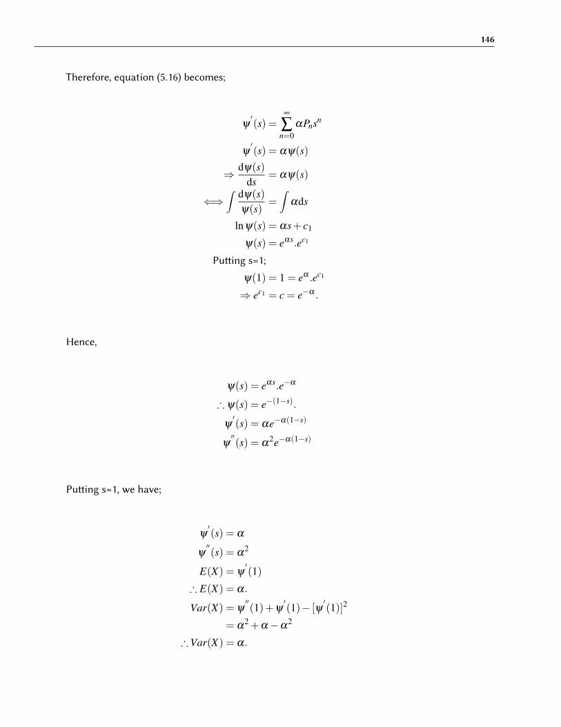
146

Therefore, equation (5.16) becomes;

ψ′(s) =

∞

∑n=0

αPnsn

ψ′(s) = αψ(s)

⇒ dψ(s)ds

= αψ(s)

⇐⇒∫ dψ(s)

ψ(s)=∫

αds

lnψ(s) = αs+ c1

ψ(s) = eαs.ec1

Pu�ing s=1;

ψ(1) = 1 = eα .ec1

⇒ ec1 = c = e−α .

Hence,

ψ(s) = eαs.e−α

∴ ψ(s) = e−(1−s).

ψ′(s) = αe−α(1−s)

ψ′′(s) = α

2e−α(1−s)

Pu�ing s=1, we have;

ψ′(s) = α

ψ′′(s) = α

2

E(X) = ψ′(1)

∴ E(X) = α.

Var(X) = ψ′′(1)+ψ

′(1)− [ψ

′(1)]2

= α2 +α−α

2

∴Var(X) = α.

147

Using Feller’s method, we sum equation (5.9) over n to obtain;

∞

∑n=0

Pn+1(n+1) =∞

∑n=0

Pnα (5.17)

Define;

M1 =∞

∑n=0

nPn =∞

∑n=0

Pn+1(1+n)

Thus, equation (5.17) becomes;

M1 = α.1

E(X) = M1

∴ E(X) = α.

Next, multiply equation (5.9) by n and a�er summing the results over n, we obtain;

∞

∑n=0

n(1+n)Pn+1 = α

∞

∑n=0

nPn (5.18)

Define;

M2 =∞

∑n=0

n2Pn =∞

∑n=0

(1+n)2Pn+1

Thus, equation (5.18) becomes;

∞

∑n=0

(1−1+n)(1+n)Pn+1 = αM1

∞

∑n=0

(1+n)2Pn+1−∞

∑n=0

(1+n)Pn+1 = αM1

M2−M1 = αM1

⇒M2 = αM1 +M1

148

But,

M1 = α

Hence, M2 = α2 +α

Thus, Var(X) = M2− [M1]2

= α2 +α−α

2

∴Var(X) = α.

(ii) When α 6= 0 and β 6= 0Then, equation (5.3) becomes;

Pn+1(1+n) = Pn(nβ +α), n = 0,1,2,3, ... (5.19)


P1 = αP0

∴ P1 = αP0.


2P2 = (β +λ )P1

P2 =α +β

2.α

1P0

∴ P2 =α(α +β )

1.2P0.


149

3P3 = (α +2β )P2

P3 =(α +2β )

3P2

⇒ P3 =(α +2β )

3.α(α +β )

1.2P0

∴ P3 =α(α +β )(α +2β )

1.2.3P0.


4P4 = (α +3β )P3

⇒ P4 =(α +3β )

4P3

⇒ P4 =(α +3β )

4.α(α +β )(α +2β )

1.2.3P0

∴ P4 =α(α +β )(α +2α)(α +3β )

1.2.3.4P0.

Therefore,When n=τ−1;Equation (5.19) becomes;

τPτ−1 = {α +(τ−1)β}Pτ−1

⇒ Pτ−1 ={α +(τ−1)β}

τPτ−1

Pτ =(

α +(τ−1)βτ

)(α +(τ−2)β

τ−1

)...(

α +3β

4

)(α +2β

3

)(α +β

2

)(α

1

)P0

Pτ = α(α +β )(α +2β )(α +3β )(α +4β )...(α +(τ−2)β )(α +(τ−1)β )P0

τ!

Pτ = βτ α

β(α

β+1)(

α

β+2)(

α

β+3)...(

α

β+ τ−2)(

α

β+ τ−1)

P0

τ!(5.20)

Pτ =β τ(α

β+ τ−1)!

(α

β−1)!τ!

P0.

∴ Pτ = βτ

α

β+ τ−1

τ

P0, τ = 0,1,2,3, ... (5.21)

150

Suppose (5.21) above is a probability mass function,Then;

∞

∑τ=0

Pτ = 1

⇒ P0 +∞

∑τ=1

Pτ = 1

That is, P0 +∞

∑τ=1

βτ

α

β+ τ−1

τ

P0 = 1

Thus, P0

{1+

∞

∑τ=1

βτ

α

β+ τ−1

τ

}= 1

Hence, P0 =1{

1+∑∞τ=1 β τ

α

β+ τ−1

τ

}

But, Pτ =β τ(α

β+ τ−1)!

(α

β−1)!τ!

P0

∴ Pτ = βτ

α

β+ τ−1

τ

P0, τ = 0,1,2,3, ...

∴ Pτ =

β τ

α

β+ τ−1

τ

∑

∞τ=0 β τ

α

β+ τ−1

τ

, τ = 0,1,2,3, ...

(5.22)

Case 1: Let ξ = α

βbe a positive integer

Then,

α

β+ τ−1

τ

=

ξ + τ−1

τ

= (−1)τ

−ξ

τ

151

⇒∞

∑τ=0

βτ

α

β+ τ−1

τ

=∞

∑τ=0

(−β )τ

−ξ

τ

= (1−β )−ξ , 0 < β < 1.

Therefore, from (5.22) we have;

Pτ =

β τ

α

β+ τ−1

τ

(1−β )−ξ

Pτ =

α

β+ τ−1

τ

βτ(1−β )ξ

∴ Pτ =

ξ + τ−1

τ

βτ(1−β )ξ ; 0 < β < 1; α > 0; τ = 0,1,2, ... (5.23)

Which is a Negative Binomial Distribution with parameters τ and 1−β .

In hypergeometric terms, we note that;

(1−β )−ξ =∞

∑τ=0

−ξ

τ

(−β )τ , ξ > 0

=∞

∑τ=0

(−1)τ

−ξ

τ

βτ

=∞

∑τ=0

ξ + τ−1

τ

βτ

=∞

∑τ=0

Γ(ξ )+ τ

Γ(ξ ).β τ

τ!

=∞

∑τ=0

(ξ + τ−1)(ξ + τ−2)(ξ + τ−3)...(ξ + τ− τ)Γ(ξ )

Γ(ξ ).β τ

τ!

152

Therefore,

(1−β )−ξ =∞

∑τ=0

(ξ + τ−1)(ξ + τ−2)(ξ + τ−3)....ξ .β τ

τ!

=∞

∑τ=0

ξ (ξ +1)...(ξ + τ−1)[([+1)...([+ τ−1)[([+1)...([+ τ−1)

β τ

τ!

∴ (1−β )−ξ =2 F1(ξ , [;[;β ).

Its probability mass function is given by;

Pr(N = τ) =

ξ + τ−1

τ

βτ(1−β )ξ ; τ = 0,1,2, ...

Hence, the pgf for a Negative Binomial Distribution is given as;

φ(z) =(1−β z)−ξ

(1−β )−ξ

∴ φ(z) = 2F1(ξ , [;[;β z)

2F1(ξ , [;[;β ).

φ′(z) =

1

2F1(ξ , [;[;β )

ddz{2F1(ξ , [;[;β z)}

=1

2F1(ξ , [;[;β )

ξ [

[.β .2F1(ξ +1, [+1;[+1;β z)

=ξ [

[β .

2F1(ξ +1, [+1;[+1;β z)

2F1(ξ , [;[;β ).

φ′′(z) =

1

2F1(ξ , [;[;β )

ξ [

[β .

ddz{2F1(ξ +1, [+1;[+1;β z)}

=1

2F1(ξ , [;[;β )

ξ [

[β .

(ξ +1)([+1)([+1)

.β .2F1(ξ +2, [+2;[+2;β z)

=ξ (ξ +1)([+1)

[([+1).β 2.

2F1(ξ +2, [+2;[+2;β z)

2F1(ξ , [;[;β ).

153

Let, Λκ =2F1(ξ +κ, [+κ;[+κ;β )

2F1(ξ , [;[;β ); κ = 1,2.

E(X) = φ′(1)

∴ E(X) =ξ [

[βΛ1.

and

Var(X) = φ′′(1)+φ

′(1)− [φ

′(1)]2

=ξ (ξ +1)[([+1)

[([+1)β

2Λ2 +

ξ [

[βΛ1− [

ξ [

[βΛ1]

2

∴Var(X) =ξ [

[βΛ1 +

ξ [

[β

2{(ξ +1)([+1)

([+1)Λ2−

ξ [

[Λ

21

}.

(a) Note that, the pgf. for a Negative Binomial distribution can be given as;

Pn =

τ +n−1

n

pτqn

Thus,

ψ(s) = E(SN) =∞

∑n=0

Pnsn

ψ(s) =∞

∑n=0

τ +n−1

n

pτqnsn

= pτ∞

∑n=0

τ +n−1

n

(qs)n

= pτ∞

∑n=0

(−1)n

−τ

n

(qs)n

= pτ(1−qs)−τ

∴ ψ(s) =( p

1−qs

)τ

. (5.24)

ψ′(s) =

τqpτ

(1−qs)τ+1

ψ′′(s) =

τ(τ +1)q2 pτ

(1−qs)τ+2

154

Pu�ing s=1;

E(X) = ψ′(1)

=τqpτ

(1−q)τ+1

∴ E(X) =τqp.

ψ′′(1) =

τ(τ +1)q2 pτ

(1−q)τ+2

=τ(τ +1)q2

p2

Var(X) = ψ′′(1)+ψ

′(1)− [ψ

′(1)]2

=τ(τ +1)q2

p2 +τqp− τ2q2

p2

=τq(q+ p)

p2

But, p+q = 1

∴Var(X) =τqp2 .

(b) Using Feller’s Method, we sum (5.19) over n to obtain;

∞

∑n=0

(1+n)Pn+1 =∞

∑n=0

(α +βn)Pn (5.25)

Define;

M1 =∞

∑n=0

nPn =∞

∑n=0

(1+n)Pn+1

and∞

∑n=0

Pn = 1.

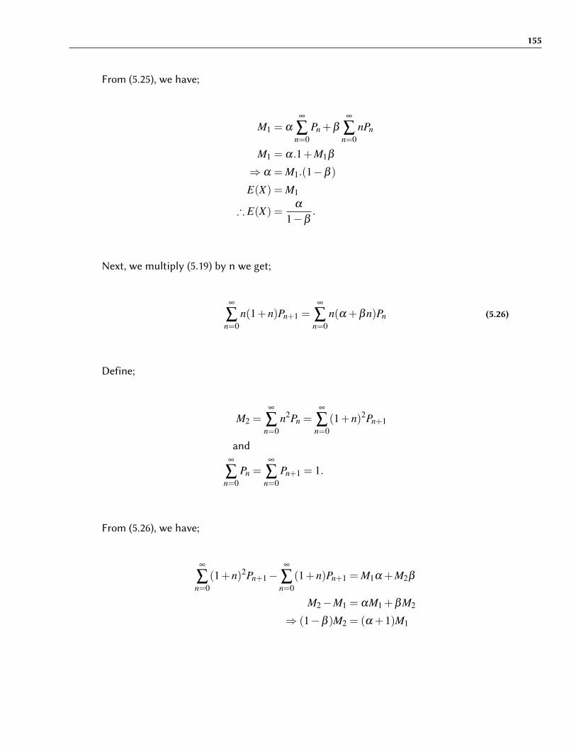
155

From (5.25), we have;

M1 = α

∞

∑n=0

Pn +β

∞

∑n=0

nPn

M1 = α.1+M1β

⇒ α = M1.(1−β )

E(X) = M1

∴ E(X) =α

1−β.

Next, we multiply (5.19) by n we get;

∞

∑n=0

n(1+n)Pn+1 =∞

∑n=0

n(α +βn)Pn (5.26)

Define;

M2 =∞

∑n=0

n2Pn =∞

∑n=0

(1+n)2Pn+1

and∞

∑n=0

Pn =∞

∑n=0

Pn+1 = 1.


∞

∑n=0

(1+n)2Pn+1−∞

∑n=0

(1+n)Pn+1 = M1α +M2β

M2−M1 = αM1 +βM2

⇒ (1−β )M2 = (α +1)M1

156

But,

α

1−β= M1

⇒ α(α +1)(1−β )2 = M2.

Var(X) = M2− [M1]2

=α(α +1)(1−β )2 −

α2

(1−β )2

=α2 +α−α2

(1−β )2

∴Var(X) =α2

(1−β )2 .

Case 2: Let ξ = α

βbe a Negative integer

Then,When ξ > 0,Equation (5.20) becomes;

Pτ = βτ(−ξ )(−ξ +1)(−ξ +2)...(−ξ + τ−1)

P0

τ!; τ = 1,2,3, ...

Pτ = (−β )τξ (ξ −1)(ξ −2)...(ξ − (τ−1))

P0

τ!

Pτ = (−β )τ

ξ

τ

P0; τ = 1,2,3, ...,ξ (5.27)

But,∞

∑τ=0

Pτ = 1

⇒ 1 =∞

∑τ=0

Pτ = P0

∞

∑τ=0

(−β )τ

ξ

τ

1 = P0{1+(−β )}ξ

∴ P0 =1

(1−β )ξ. (5.28)

157


Pτ =

(−β )τ

ξ

τ

(1−β )ξ

∴ Pτ =

ξ

τ

( −β

1−β

)τ( 11−β

)ξ−τ

; τ = 0,1,2,3, ...,ξ (5.29)

Which is a Binomial Distribution with parameters −α

β= ξ , −β

1−β; where α

βis a negative

integer and β < 0 ⇒ α > 0.Note that;

(1+β )ξ =∞

∑τ=0

ξ

τ

βτ

= 1+

ξ

1

β1 +

ξ

2

β2 +

ξ

3

β3 + ...+

ξ

ξ

βξ

= 1+ξ

1!β

1 +ξ (ξ −1)

2!β

2 +ξ (ξ −1)(ξ −2)

3!β

3 + ...+ξ (ξ −1)...2.1.β ξ

ξ !

= 1+(−1)ξ (−1)β

1!+(−1)2

ξ (ξ −1)(−1)2 β 2

2!+(−1)3

ξ (ξ −1)(ξ −2)(−1)3 β 3

3!+ ...

+(−1)ξξ (ξ −1)...2.1.(−ξ )ξ β ξ

ξ !

= 1+(−ξ )

1(−β )

1!+

(−ξ )(−ξ +1)1.21.2

(−β )ξ

2!+ ...

+(−ξ )(−ξ +1)...(−ξ +ξ +1)

1.2.3...ξ1.2.3...ξ

(−β )ξ

ξ !=2 F1(−ξ ,1;1;−β ).

158

Its probability mass function is given by;

Pr(N = τ) =

ξ

τ

β τ

(1+β )ξ

=

ξ

τ

( β

(1+β )

)τ( 1(1+β )

)ξ−τ

; τ = 0,1,2,3, ...,ξ .

Which is a binomial distribution with parameters ξ and β

(1+β ) .

The pgf. for a Binomial Distribution in hypergeometric terms is expressed as;

φ(z) =(1+β z)ξ

(1+β )ξ

∴ φ(z) = 2F1(−ξ ;1;1;−β z)

2F1(−ξ ;1;1;−β ).

φ′(z) =

1

2F1(−ξ ;1;1;−β )

ddz{2F1(−ξ ;1;1;−β z)}

=1

2F1(−ξ ;1;1;−β ).ξ .β .2F1(−ξ +1;1+1;1+1;−β z)

= ξ β2F1(−ξ +1;2;2;−β z)

2F1(−ξ ;1;1;−β ).

φ′′(z) =

1

2F1(−ξ ;1;1;−β ).ξ β .

ddz{2F1(−ξ +1;2;2;−β z)}

=1

2F1(−ξ ;1;1;−β ).ξ β .

(−ξ +1)22

.2F1(−ξ +2;2+1;2+1;−β z)

=−ξ (−ξ +1)β 2

22F1(−ξ +2;3;3;−β z)

2F1(−ξ ;1;1;−β ).

Let, Λκ =2F1(−ξ +κ;1+κ;1+κ;−β )

2F1(−ξ ;1;1;−β ); κ = 1,2.

E(X) = φ′(1)

∴ E(X) = ξ βΛ1.

and

Var(X) = φ′′(1)+φ

′(1)− [φ

′(1)]2

=−ξ (−ξ +1)2β 2

2Λ2 +ξ βΛ1− [ξ βΛ1]

2

∴Var(X) = ξ βΛ1 +ξ β2{(ξ −1)2

2Λ2−ξ Λ

21}.

159

5.2.2 Obtaining Means and Variance of Katz probability


∞

∑n=0

(1+n)Pn+1sn =∞

∑n=0

(α +βn)Pnsn (5.30)

Define; ψ(s) =∞

∑n=0

Pnsn

ψ′(s) =

∞

∑n=0

nPnsn

ψ′(s) =

∞

∑n=0

(n+1)Pn+1sn


ψ′(s) = α

∞

∑n=0

Pnsn +β

∞

∑n=0

nPnsn

ψ′(s) = αψ(s)+β s

∞

∑n=0

nPnsn−1

ψ′(s) = αψ(s)+β sψ

′(s)

⇐⇒ (1−β s)ψ′(s) = αψ(s)

⇒ (1−β s)dψ(s)

ds= αψ(s)∫ dψ(s)

ψ(s)=∫

α

1−β sds

lnψ(s) =α

−βln(1−β s)+ lnc

lnψ(s) = ln(1−β s)α

−β + lnc

lnψ(s) = lnc(1−β s)α

−β

ψ(s) = c1(1−β s)α

−β (5.31)

160

Pu�ing s=1;

ψ(s) = 1 = c1(1−β )α

−β

⇒ 1 = c1(1−β )α

−β

⇒ c1 =1

(1−β )α

−β

∴ c1 = (1−β )α

β

∴ ψ(s) =(1−β s

1−β

)−α

β

∴ ψ(s) =( 1−β

1−β s

)α

β

. (5.32)

Let ξ = α

βbe a positive integer,

Then,

ψ(s) =(1−β s

1−β

)−ξ

∴ ψ(s) =( 1−β

1−β s

)ξ

.

Let 1−β = p and p+q = 1Then,

ψ(s) =( p

1−qs

)ξ

.

Which is the pgf. for a Negative binomial distribution with parameters ξ > 0 and p= 1−β .

From (5.32), the pgf. is given as;

ψ(s) =( 1−β

1−β s

)α

β

161

therefore;

ψ′(s) =

α

1−β sψ(s)

ψ′′(s) =

dds

(α

1−β sψ(s)

)⇒ ψ

′′(s) =

αψ′(s)

1−β s+

αβψ(s)(1−β s)2

Pu�ing s=1;

ψ′(1) =

α

1−βψ(1)

But, ψ(1) = 1

E(X) = ψ′(1)

∴ E(X) =α

1−β.

ψ′′(1) =

αψ′(1)

1−β+

αβψ(1)(1−β )2

=α2 +αβ

(1−β )2

Var(X) = ψ′′(1)+ψ

′(1)− [ψ

′(1)]2

=α2 +αβ

(1−β )2 +α

1−β− α2

(1−β )2

∴Var(X) =α

(1−β )2 .

5.3 Extension of Recursive Model by Tripathi - Gurland (1977)

Gurland and Tripathi (1975) and Tripathi and Gurland (1977) Extended Katz Family ofdistributions.The relationship between the probabilities has the form:

Pn+1

Pn=

α +βnγ +n

(**)

⇒ (n+ γ)Pn+1 = (βn+α)Pn (5.33)

162

Proposition 5.2

Pn+1

Pn=

α +βnγ +n

; n = 0,1,2,3, ...

ProofSolving equation (5.33) iteratively, we have;When n=0;Equation (5.33) becomes;

γP1 = αP0

⇒ P1 =α

γP0

∴ P1 =α

γP0 (5.34)


(1+ γ)P2 = (β +α)P1

⇒ P2 =β +α

1+ γP1

∴ P2 =β +α

1+ γP1.

Substitution (5.34) in equation (5.35), we have;

P2 =β +α

1+ γ

α

γP0

∴ P2 =α(α +β )

γ(γ +1)P0. (5.36)


163

(γ +2)P3 = (α +2β )P2 (5.37)


(γ +2)P3 = (α +2β )α(α +β )

γ(γ +1)P0

⇒ P3 =(α +2β )(α +β )α

(γ +2)(γ +1)γP0

∴ P3 =α(α +β )(α +2β )

γ(γ +1)(γ +2)P0.

By Mathematical Induction, we have;

P4 =α(α +β )(α +2β )(α +3β )

γ(γ +1)(γ +2)(γ +3)P0,

P5 =α(α +β )(α +2β )(α +3β )(α +4β )

γ(γ +1)(γ +2)(γ +3)(γ +4)P0,

.

.

.

Pn =α(α +β )(α +2β )(α +3β )...(α +n−1)

γ(γ +1)(γ +2)(γ +3)...(γ +n−1)P0.

(5.38)

But,∞

∑n=0

Pn = 1

⇒ P0 +P1 +P2 +P3 + ...+Pn + ...= 1

P0

{1+

α

γ+

α(α +β )

γ(γ +1)+ ...

}= 1

∴ P0 =1{

1+ α

γ+ α(α+β )

γ(γ+1) + ...}

∴ Pn =α(α +β )(α +2β )(α +3β )...(α +n−1)

γ(γ +1)(γ +2)(γ +3)...(γ +n−1).

1{1+ α

γ+ α(α+β )

γ(γ+1) + ...}

164


Pn+1 =α(α +β )(α +2β )...(α +n−1)(α +nβ )

γ(γ +1)(γ +2)...(γ +n−1)(γ +n)P0.

∴Pn+1

Pn=

α(α +β )(α +2β )...(α +n−1)(α +nβ )

γ(γ +1)(γ +2)...(γ +n−1)(γ +n).

γ(γ +1)(γ +2)...(γ +n−1)α(α +β )(α +2β )...(α +n−1)

∴Pn+1

Pn=

α +nβ

γ +n; as required.

Multiplying (5.33) by sn and sum the results over n, we have;

∞

∑n=0

(γ +n)Pn+1sn =∞

∑n=0

(α +βn)Pnsn

γ

∞

∑n=0

Pn+1sn +∞

∑n=0

nPn+1sn = α

∞

∑n=0

Pnsn +β

∞

∑n=0

nPnsn (5.39)

Define; ψ(s) =∞

∑n=0

Pnsn

ψ′(s) =

∞

∑n=0

nPnsn−1 =∞

∑n=0

(n+1)Pnsn


γψ(s)+∞

∑n=0

(n+1−1)Pn+1sn = αψ(s)+β sψ′(s)

γψ(s)+∞

∑n=0

(n+1)Pn+1sn−∞

∑n=0

Pn+1sn = αψ(s)+β sψ′(s)

γψ(s)+ψ′(s)−ψ(s) = αψ(s)+β sψ

′(s)

(1−β s)ψ′(s) = (α +1− γ)ψ(s)

(1−β s)dψ(s)

ds= (α +1− γ)ψ(s)∫ dψ(s)

ψ(s)=∫

α +1− γ

1−β sds

lnψ(s) =∫

α

1−β sds+

∫ 11−β s

ds−∫

γ

1−β sds

lnψ(s) =α

−βln(1−β s)+

1−β

ln(1−β s)− γ

−βln(1−β s)+ lnc

165

Therefore,

lnψ(s) = ln(1−β s)α

−β + ln(1−β s)1−β − ln(1−β s)

γ

−β + lnc

lnψ(s) = lnc1. ln(1−β s)α

−β . ln(1−β s)1−β .

1

ln(1−β s)γ

−β

∴ ψ(s) = c1.(1−β s)α

−β .(1−β s)1−β .

1

(1−β s)γ

−β

Pu�ing s=1;

ψ(1) = 1 = c1(1−β )

α

−β .(1−β )1−β

(1−β s)γ

−β

⇒ c1 =(1−β s)

γ

−β

(1−β )α

−β .(1−β )1−β

∴ ψ(s) =(1−β s)

−α

β (1−β s)−1β (1−β s)

−γ

β

(1−β )−α

β (1−β )−1β (1−β )

−γ

β

Thus, from gauss hypergeometric series, we have;

2F1(α

β,1;γ;β ) = 1+

α

β.1

γ+

β

1!+

α

β(α

β+1)1(1+1)

γ(γ +1)β 2

2!+ ...+

(α

β+n−1)(1+n−1)

(γ +n−1)β n

n!; γ > 0

=∞

∑n=0

α

β(α

β+1)...(α

β+n−1)1(1+1)(1+2)...(1+n−1)

γ(γ +1)(γ +2)...(γ +n−1)β n

n!

=∞

∑n=0

(α

β+n−1)...(α

β+1)α

β(1+n−1)...(1+2)(1+1)1

(γ +n−1)...(γ +2)(γ +1)γβ n

n!

=∞

∑n=0

Γ(α

β+n)Γ(1+n)

Γ(γ +n).

Γ(γ)

Γ(α

β)Γ(1)

β n

n!


1 =∞

∑n=0

Γ(α

β+n)Γ(1+n)

Γ(γ +n).

Γ(γ)

Γ(α

β)Γ(1)

.1

2F1(α

β,1;γ;β )

β n

n!

166

Hence,

Pn = Prob.(N = n)

=∞

∑n=0

Γ(α

β+n)Γ(1+n)

Γ(γ +n).

Γ(γ)

Γ(α

β)Γ(1)

.1

2F1(α

β,1;γ;β )

β n

n!

The pgf. is given as;

φ(z) =∞

∑n=0

Pnzn

φ(z) =∞

∑n=0

Γ(α

β+n)Γ(1+n)

Γ(γ +n).

Γ(γ)

Γ(α

β)Γ(1)

.(β z)n

n!.

1

2F1(α

β,1;γ;β )

∴ φ(z) =2F1(

α

β,1;γ;β z)

2F1(α

β,1;γ;β )

.

Which is the probability generating function of an extended hypergeometric function.

φ′(z) =

1

2F1(α

β,1;γ;β )

ddz{2F1(

α

β,1;γ;β z)}

=1

2F1(α

β,1;γ;β )

α

β.1γ.β{ 1

2F1(α

β+1,1+1;γ +1;β z)

}

=α

β

1γ.β

2F1(α

β+1,2;γ +1;β z)

2F1(α

β,1;γ;β )

φ′′(z) =

1

2F1(α

β,1;γ;β )

α

β

1γ

βddz{2F1(

α

β+1,2;γ +1;β z)}

=1

2F1(α

β,1;γ;β )

α

β

1γ

β .(α

β+1)2

γ +1β{2F1(

α

β+1,2;γ +1;β z)}

=

α

β(α

β+1)2

γ(γ +1)β

2 2F1(α

β+2,2+1;γ +2;β z)

2F1(α

β,1;γ;β )

.

Let, Λκ =2F1(

α

β+κ,1+κ;γ +κ;β )

2F1(α

β,1;γ;β )

; κ = 1,2.

E(X) = φ′(1)

∴ E(X) =α

β

1γ

βΛ1.

167

and

Var(X) = φ′′(1)+φ

′(1)− [φ

′(1)]2

=α

β(α

β+1)

2γ

β2Λ2 +

α

β

1γ

Λ1−{α

β

1γ

Λ1}2

∴Var(X) =α

β

1γ

βΛ1 +α

β

1γ

β2{(α

β+1)

2(γ +1)

Λ2−α

β

1γ

βΛ21}.

5.4 Family of Distributions by Jewell and Sundt

Sundt and Jewell (1981) and Willmot (1988) have created the sundt and jewell family ofdistributions which is a modified form of the Katz family. Their recurrence relationshipfor the probability is given by;Proposition 5.3

Pn+1

Pn=

a+b+an1+n

; n = 0,1,2, ... (5.40)

⇒ (1+n)Pn+1 = (a+b+an)Pn (5.41)

ProofSolving (5.41) iteratively, we have;When n=0; Equation (5.41) becomes;

P1 = (a+b)P0

∴ P1 = (a+b)P0 (5.42)


2P2 = (2a+b)P1 (5.43)

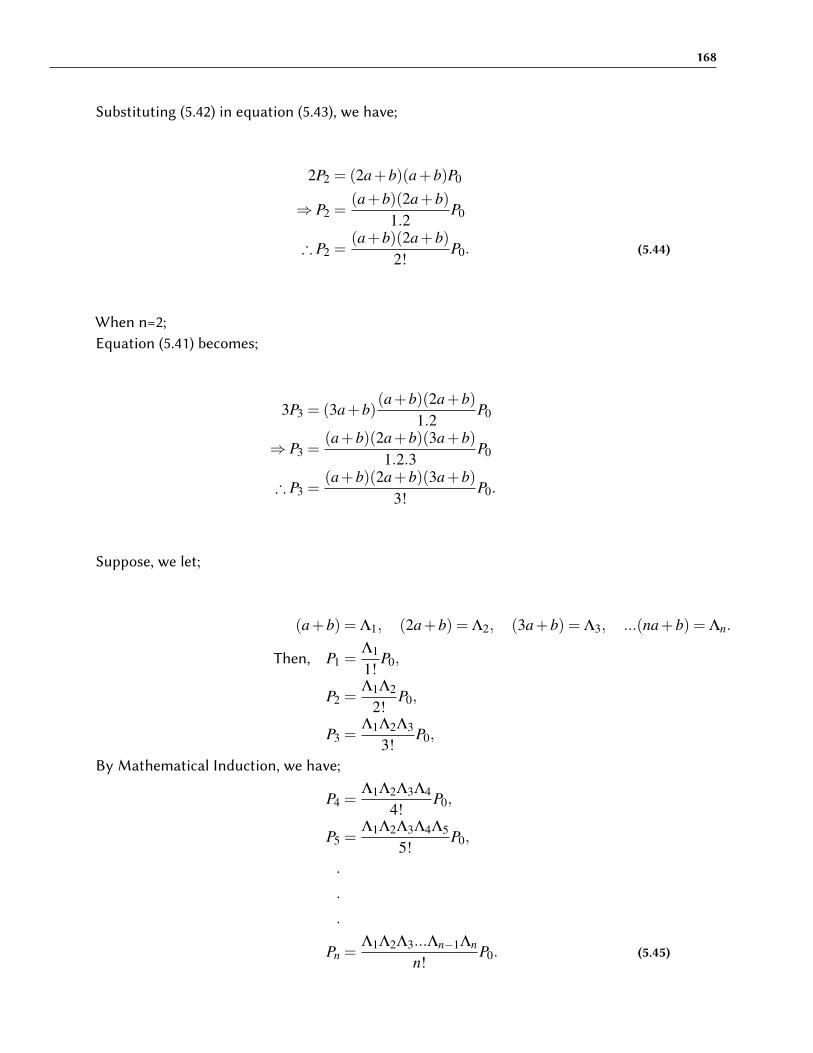
168


2P2 = (2a+b)(a+b)P0

⇒ P2 =(a+b)(2a+b)

1.2P0

∴ P2 =(a+b)(2a+b)

2!P0. (5.44)


3P3 = (3a+b)(a+b)(2a+b)

1.2P0

⇒ P3 =(a+b)(2a+b)(3a+b)

1.2.3P0

∴ P3 =(a+b)(2a+b)(3a+b)

3!P0.

Suppose, we let;

(a+b) = Λ1, (2a+b) = Λ2, (3a+b) = Λ3, ...(na+b) = Λn.

Then, P1 =Λ1

1!P0,

P2 =Λ1Λ2

2!P0,

P3 =Λ1Λ2Λ3

3!P0,


P4 =Λ1Λ2Λ3Λ4

4!P0,

P5 =Λ1Λ2Λ3Λ4Λ5

5!P0,

.

.

.

Pn =Λ1Λ2Λ3...Λn−1Λn

n!P0. (5.45)

169

Therefore, from (5.45) we have;

Pn+1 =Λ1Λ2Λ3...ΛnΛn+1

(n+1)!P0.

Pn+1

Pn=

Λ1Λ2Λ3...Λn−1ΛnΛn+1

(n+1).n!.

n!Λ1Λ2Λ3...Λn−1Λn

∴Pn+1

Pn=

Λn+1

n+1

∴Pn+1

Pn=

a+b+ann+1

, as required.

Multiplying (5.41) by sn and sum the results over n to obtain;

∞

∑n=0

(n+1)Pn+1sn =∞

∑n=0

(a+b+an)Pnsn

ψ′(s) = a

∞

∑n=0

Pnsn +b∞

∑n=0

Pnsn +as∞

∑n=0

nPnsn−1

ψ′(s) = aψ(s)+bψ(s)+asψ

′(s)

⇒ (1−as)ψ′(s) = (a+b)ψ(s)

(1−as)dψ(s)

ds= (a+b)ψ(s)∫ dψ(s)

ψ(s)=∫ a+b

1−asds

lnψ(s) =a+b−a

ln(1−as)+ lnc

lnψ(s) = lnc ln(1−as)a+b−a

ψ(s) = c1(1−as)a+b−a

Pu�ing s=1;

ψ(1) = 1 = c1(1−a)a+b−a

∴ c1 = (1−a)a+b

a .

170

Therefore;

ψ(s) =(1−as

1−a

)−(a+b)a

∴ ψ(s) =( 1−a

1−as

) (a+b)a

.

ψ′(s) =

a+b1−as

.( 1−a

1−as

) (a+b)a

ψ′′(s) =

a+b1−as

.a+b1−as

( 1−a1−as

) (a+b)a

+(a+b)a(1−as)2

( 1−a1−as

) (a+b)a

E(X) = ψ′(1)

∴ E(X) =a+b1−a

.

Var(X) = ψ′′(1)+ψ

′(1)− [ψ

′(1)]2

=[(a+b)2

(1−a)2 +a(a+b)(1−a)2

]+

a+b1−a

− (a+b)2

(1−a)2

=(a+b)2 +a(a+b)(a+b)(1−a)− (a+b)2

(1−a)2

=a2 +ab+a−a2 +b−ab

(1−a)2

∴Var(X) =a+b

(1−a)2 .

Using Feller’s method, we sum (5.41) over n to obtain;

∞

∑n=0

(n+1)Pn+1 =∞

∑n=0

(a+b+an)Pn

M1 = a∞

∑n=0

Pn +b∞

∑n=0

Pn +a∞

∑n=0

nPn

M1 = a+b+aM1

(1−a)M1 = (a+b)

⇒M1 =a+b1−a

E(X) = M1

∴ E(X) =a+b1−a

.

171

Next, we multiply (5.41) by n and sum to obtain;

∞

∑n=0

(n+1)nPn+1 =∞

∑n=0

n(a+b+an)Pn

∞

∑n=0

(n+1)(n+1−1)Pn+1 = a∞

∑n=0

nPn +b∞

∑n=0

nPn +a∞

∑n=0

+a∞

∑n=0

n2Pn

∞

∑n=0

(1+n)2Pn+1−∞

∑n=0

(1+n)Pn+1 = aM1 +bM1 +aM2

M2−M1 = aM1 +bM1 +aM2

(1−a)M2 = (a+b+1)M1

∴ M2 =(a+b)(a+b+1)

(1−a)2

Var(X) = M2−{M1}2

=(a+b)(a+b+1)

(1−a)2 −{a+b

1−a

}2

=a2 +ab+ab+b2 +a+b−a2−2ab−b2

(1−a)2

∴Var(X) =a+b

(1−a)2 .

5.5 Irwin (1963) Recursive Model

From equation (**) in section 5.3 above, when β = 1 and γ > 1, it belongs to Katz classfamily and has been presented by Irwin (1963) as;Proposition 5.4

Pn+1

Pn=

n+α

n+ γ

(n+ γ)Pn+1 = (n+α)Pn (5.46)

ProofSolving (5.46) iteratively, we have;When n=0;Equation (5.46) becomes;

172

γP1 = αP0

⇒ P1 =α

γP0

∴ P1 =α

γP0. (5.47)


(γ +1)P2 = (α +1)P1 (5.48)


(γ +1)P2 = (α +1)α

γP0

⇒ P2 =α(α +1)γ(γ +1)

P0

∴ P2 =α(α +1)γ(γ +1)

P0. (5.49)


(γ +2)P3 = (α +2)P2 (5.50)


(γ +2)P3 = (α +2)α(α +1)γ(γ +1)

P0

⇒ P3 =α(α +1)(α +2)γ(γ +1)(γ +2)

P0

∴ P3 =α(α +1)(α +2)γ(γ +1)(γ +2)

P0.

173

Suppose we let Λ1 =α

γ, Λ2 =

α+1γ+1 , Λ3 =

α+2γ+2 , ..., Λn =

α+n−1γ+n−1 .

Then;

P1 = Λ1P0,

P2 = Λ1Λ2P0,

P3 = Λ1Λ2Λ3P0.

Therefore, by Mathematical Induction, we have;

P4 = Λ1Λ2Λ3Λ4P0,

P5 = Λ1Λ2Λ3Λ4Λ5P0,

.

.

.

Pn = Λ1Λ2Λ3...Λn−1ΛnP0. (5.51)

But,

P0 +P1P2 +P3 + ...= 1

⇒ P0 +Λ1P0 +Λ1Λ2P0 +Λ1Λ2Λ3P0 + ...+Λ1Λ2Λ3...Λn−1ΛnP0 = 1

P0

{1+Λ1 +Λ1Λ2 +Λ1Λ2Λ3 + ...+Λ1Λ2Λ3...Λn−1Λn

}= 1

∴ P0 =1{

1+Λ1 +Λ1Λ2 +Λ1Λ2Λ3 + ...} .

∴ Pn = Λ1Λ2Λ3...Λn.1{

1+Λ1 +Λ1Λ2 + ...} .


Pn+1 = Λ1Λ2Λ3...ΛnΛn+1P0.

174

Therefore,

Pn+1

Pn= Λ1Λ2Λ3...ΛnΛn+1.

1Λ1Λ2Λ3...Λn−1Λn

∴Pn+1

Pn= Λn+1

∴Pn+1

Pn=

α +nγ +n

, as required.

Using the probability generating function techniques, we multiply (5.46) by sn and sumthe results over n to obtain;

∞

∑n=0

(γ +n)Pn+1sn =∞

∑n=0

(α +n)Pnsn

γ1s

∞

∑n=0

Pn+1sn+1 +∞

∑n=0

nPn+1sn = α

∞

∑n=0

Pnsn + s∞

∑n=0

nPnsn−1

γ

sψ(s)+

∞

∑n=0

[(n+1)−1]Pn+1sn = αψ(s)+ sψ′(s)

γ

sψ(s)+

∞

∑n=0

(n+1)Pn+1sn− 1s

∞

∑n=0

Pn+1sn+1 = αψ(s)+ sψ′(s)

γ

sψ(s)+ψ

′(s)− 1

sψ(s) = αψ(s)+ sψ

′(s)

γψ(s)+ sψ′(s)−ψ(s) = sαψ(s)+ s2

ψ′(s)

s(1− s)ψ′(s) = (γ +αs+ s)ψ(s)

s(1− s)dψ(s)

ds= (γ +αs+ s)ψ(s)∫ dψ(s)

ψ(s)=∫

(γ +αs+ s)s(1− s)

ds

lnψ(s) =∫

γ

s(1− s)ds+

∫α

(1− s)ds+

∫ 1(1− s)

ds

∴ ψ(s) = (1− s)−α .(1− s)−γ .(1− s)−1.

175

Its probability generating function in hypergeometric terms is given by;

φ(z) = 2F1(α,1;γ;z)

2F1(α,1;γ;1).

φ′(z) =

α.1γ

.2F1(α +1,2;γ +1;z)

2F1(α,1;γ;1)

φ′′(z) =

α(α +1).1(2)γ(γ +1)

.2F1(α +2,3;γ +2;z)

2F1(α,1;γ;1)

=2α(α +1)γ(γ +1)

.2F1(α +2,3;γ +2;z)

2F1(α,1;γ;1)

Let, Λκ =2F1(α +κ,1+κ;γ +κ;1)

2F1(α,1;γ;1); κ = 1,2.

E(X) = φ′(1)

∴ E(X) =α

γΛ1.

Var(X) = φ′′(1)+φ

′(1)− [φ

′(1)]2

=2α(α +1)γ(γ +1)

Λ2 +α

γΛ1− [

α

γΛ1]

2

∴Var(X) =α

γΛ1 +

α

γ

{2(α +1)(γ +1)

Λ2−α

γΛ

21

}.

5.6 Yousry and Srivastava (1987) Recursive Model

The hyper-negative binomial distribution of Yousry and Srivastava (1987) belongs to theextended Katz family. The ratio of successive probabilities is;Proposition 5.5

Pn+1

Pn=

(r+n)qθ +n

, 0 < q < 1, r > 0, θ > 0

⇒ (θ +n)Pn+1 = (r+n)qPn (5.52)


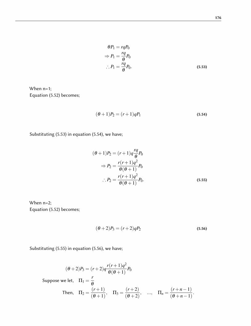
176

θP1 = rqP0

⇒ P1 =rqθ

P0

∴ P1 =rqθ

P0. (5.53)


(θ +1)P2 = (r+1)qP1 (5.54)


(θ +1)P2 = (r+1)qrqθ

P0

⇒ P2 =r(r+1)q2

θ(θ +1)P0

∴ P2 =r(r+1)q2

θ(θ +1)P0. (5.55)


(θ +2)P3 = (r+2)qP2 (5.56)


(θ +2)P3 = (r+2)qr(r+1)q2

θ(θ +1)P0

Suppose we let, Π1 =rθ

Then, Π2 =(r+1)(θ +1)

, Π3 =(r+2)(θ +2)

, ..., Πn =(r+n−1)(θ +n−1)

.

177

Therefore,

P1 = Π1qP0,

P2 = Π1Π2q2P0,

P3 = Π1Π2Π3q3P0,


P4 = Π1Π2Π3Π4q4P0,

P5 = Π1Π2Π3Π4Π5q5P0,

.

.

.

Pn = Π1Π2Π3...Πn−1ΠnqnP0. (5.57)


Pn+1 = Π1Π2Π3...ΠnΠn+1qn+1P0.

Pn+1

Pn= Π1Π2Π3...ΠnΠn+1q.qn.

1Π1Π2Π3...Πnqn

∴Pn+1

Pn= qΠn+1.

∴Pn+1

Pn=

(r+n)q(θ +n)

, as required.

Its probability generating function in terms of hyper-geometric function is given by;

φ(z) = 2F1(1,r;θ ;qz)

2F1(1,r;θ ;q).

φ′(z) =

r.1θ

q.2F1(1+1,r+1;θ +1;qz)

2F1(1,r;θ ;q)

=rθ

q.2F1(2,r+1;θ +1;qz)

2F1(1,r;θ ;q)

φ′′(z) =

2r(r+1)θ(θ +1)

q2.2F1(2+1,r+2;θ +2;qz)

2F1(1,r;θ ;q)

178

Let,

Λκ =2F1(1+κ,r+κ;θ +κ;q)

2F1(1,r;θ ;q); κ = 1,2.

E(X) = φ′(1)

∴ E(X) =rqθ

Λ1.

Var(X) = φ′′(1)+φ

′(1)− [φ

′(1)]2

=2r(r+1)q2

θ(θ +1)Λ2 +

rqθ

Λ1− [rqθ

Λ1]2

∴Var(X) =rqθ

Λ1 +rq2

θ

{2(r+1)(θ +1)

Λ2−rθ

Λ21

}.

6 CROW-BARDWELL RECURSIVE MODEL AND ITSEXTENSION IN BIRTH AND DEATH PROCESSESAT EQUILIBRIUM

6.1 Introduction

Let Pn be the distribution of population size n, λn and µn is the birth (death) rate of thepopulation.The Pearson’s di�erential equation given by;

Pn+1

Pn=

P(n)Q(n)

where P(n) and Q(n) are polynomials.

The Bardwell-Crow Recursive relations is given by;

Pn+1

Pn=

α

γ +n; n = 0,1,2, ...

6.2 Bardwell-Crow (1964) Model

To obtain the hyper-Poisson Distribution of Bardwell and Crow (1964) and Crow andBardwell (1965), we let β → ∞, in equation (**) in section 5.3.Hence, we have;Proposition 6.1

Pn+1

Pn=

α

n+ γ; n = 0,1,2,3,4, ...

⇒ (n+ γ)Pn+1 = αPn (6.1)

ProofSolving (6.1) iteratively, we have;

181


γP1 = αP0

⇒ P1 =α

γP0

∴ P1 =α

γP0. (6.2)


(γ +1)P2 = αP1 (6.3)


(γ +1)P2 =α2

γP0

⇒ P2 =α2

γ(γ +1)P0

∴ P2 =α2

γ(γ +1)P0. (6.4)


(γ +2)P3 = αP2 (6.5)


(γ +2)P3 =α3

γ(γ +1)P0

∴ P3 =α3

γ(γ +1)(γ +2)P0.

182

Suppose we let α

γ= Φ1.

Then,

Φ2 =α

γ +1, Φ3 =

α

γ +2, Φ4 =

α

γ +3... Φn =

α

γ +n−1.

Therefore,

P1 = Φ1P0,

P2 = Φ1Φ2P0,

P3 = Φ1Φ2Φ3P0.


P4 = Φ1Φ2Φ3Φ4P0,

P5 = Φ1Φ2Φ3Φ4Φ5P0,

.

.

.

Pn = Φ1Φ2Φ3...Φn−1ΦnP0. (6.6)

But,

∞

∑n=0

Pn = 1

⇒ P0 +P1 +P2 +P3 + ...= 1

P0 +Φ1P0 +Φ1Φ2P0 +Φ1Φ2Φ3P0 + ...= 1

P0

{1+Φ1 +Φ1Φ2 +Φ1Φ2Φ3 + ...

}= 1

∴ P0 =1{

1+Φ1 +Φ1Φ2 +Φ1Φ2Φ3 + ...} .

∴ Pn = Φ1Φ2Φ3...Φn−1Φn.1{

1+Φ1 +Φ1Φ2 +Φ1Φ2Φ3 + ...} .

183

From (6.6), we get;

Pn+1 = Φ1Φ2Φ3...ΦnΦn+1P0.

Pn+1

Pn= Φ1Φ2Φ3...ΦnΦn+1.

1Φ1Φ2Φ3...Φn

.

∴Pn+1

Pn= Φn+1.

∴Pn+1

Pn=

α

n+ γ, as required.

Multiplying (6.1) by sn and sum the results over n, we have;

∞

∑n=0

(γ +n)Pn+1sn = α

∞

∑n=0

Pnsn

γ

∞

∑n=0

Pn+1sn +∞

∑n=0

nPn+1sn = αψ(s)

γψ(s)+∞

∑n=0

(n+1−1)Pn+1sn = αψ(s)

γψ(s)+∞

∑n=0

(n+1)Pn+1sn−∞

∑n=0

Pn+1sn = αψ(s)

γψ(s)+ψ′(s)−ψ(s) = αψ(s)

ψ′(s) = (α− γ +1)ψ(s)

dψ(s)ds

= (α− γ +1)ψ(s)∫ dψ(s)ψ(s)

=∫(α− γ +1)ds

lnψ(s) =∫

αds+∫

ds−∫

γds

lnψ(s) = αs+ s− γs+ c

ψ(s) = eαs+s−γs.ec

Pu�ing s=1; ψ(1) = 1 = eα+1−γ .ec1

⇒ c1 = e−(α+1−γ).

∴ ψ(s) =e(α+1−γ)s

e(α+1−γ).

184


1F1(1;γ;α) = 1+1γ

α

1!+

1(1+1)γ(γ +1)

α2

2!+

1(1+1)(1+2)γ(γ +1)(γ +2)

α3

3!+ ...

=∞

∑n=0

1(1+1)(1+2)...(1+n−1)γ(γ +1)(γ +2)...(γ +n−1)

αn

n!

=∞

∑n=0

(1+n−1)(1+n−2)...(1+2)(1+1)1(γ +n−1)(γ +n−2)...(γ +2)(γ +1)γ

Γ(1)Γ(γ)

.Γ(γ)

Γ(1).αn

n!

=∞

∑n=0

Γ(1+n)Γ(γ +n)

.Γ(γ)

Γ(1).αn

n!


1 =∞

∑n=0

Γ(1+n)Γ(γ +n)

.Γ(γ)

Γ(1).

1

1F1(1;γ;α).αn

n!

Thus,

Pn = Prob(N = n)

=∞

∑n=0

Γ(1+n)Γ(γ +n)

.Γ(γ)

Γ(1).

1

1F1(1;γ;α).αn

n!; n = 0,1,2, ... γ > 0, α > 0.

The probability generating function is given by;

φ(z) =∞

∑n=0

Pnzn

φ(z) =∞

∑n=0

∞

∑n=0

Γ(1+n)Γ(γ +n)

.Γ(γ)

Γ(1).(αz)n

n!.

1

1F1(1;γ;α)

∴ φ(z) = 1F1(1;γ;αz)

1F1(1;γ;α).

185

This implies that;

φ′(z) =

1

1F1(1;γ;α)

ddz{1F1(1;γ;αz)}

=1

1F1(1;γ;α)

α

γ.1F1(1+1;γ +1;αz)

=α

γ

1F1(2;γ +1;αz)

1F1(1;γ;α).

φ′′(z) =

1

1F1(1;γ;α).α

γ.

ddz{1F1(2;γ +1;αz)}

=1

1F1(1;γ;α).α

γ.

2α

γ +1.1F1(2+1;γ +2;αz)

=2α2

γ(γ +1)1F1(3;γ +2;αz)

1F1(1;γ;α).

Let, Λκ =1F1(1+κ;γ +κ;α)

1F1(1;γ;α), κ = 1,2.

E(X) = φ′(1)

∴ E(X) =α

γΛ1.

Var(X) = φ′′(1)+φ

′(1)− [φ

′(1)]2

=2α2

γ(γ +1)Λ2 +

α

γΛ1− [

α

γΛ1]

2

∴Var(X) =α

γΛ1 +

α2

γ

{ 2γ +1

Λ2−1γ

Λ21

}.

6.3 Special Cases and Properties

Case1: When α = θ and γ = r

Sta� (1964, 1967) defined the displaced Poisson distribution as a le�-truncated Poissondistribution that has been "displaced" which corresponds to the displaced distribution;

Prob(N = n) =θ n+r+1

(n+ r+1)!

{ ∞

∑j=r+1

α j

j!

}−1, n = 0,1,2, ... (6.7)

186

Using recurrence relation, Sta� also obtained the distribution;

Prob[N = n+1] =θ

r+nProb[N = n], n = 1,2, ...

where r is a positive integer.

Suppose we let the partial sum be given by;

z =θ r+1

(r+1)!+

θ r+2

(r+2)!+

θ r+3

(r+3)!+ · · ·

=∞

∑n=0

θ n+r+1

(n+ r+1)!

∴ 1 =∞

∑n=0

θ n+r+1

(n+ r+1)! z

∴ f (n) =θ n+r+1

(n+ r+1)!∑∞n=0

θ n+r+1

(n+r+1)!

for n = 0,1,2, · · · ;θ > 0 (6.8)

f (n) =θ n+r+1

(n+ r+1)!∑∞n=0

θ n+r+1

(n+r+1)!

=θ n+r+1

Γ(n+ r)1

∑∞n=0

θ n+r+1

Γ(n+r)

=θ n

Γ(n+ r)1

∑∞n=0

θ n

Γ(n+r)

=θ n

Γ(n+ r)1

∑∞n=0

θ n

n!n!

Γ(n+r)

=θ n

Γ(n+ r)1

∑∞n=0

Γ(1+n)Γ(n+r)

θ n

n!

=θ n

Γ(n+ r)1

∑∞n=0

Γ(1+n)Γ(n+r)

θ n

n!

=θ n

Γ(n+ r)Γ(r)Γ(r)

1

∑∞n=0

Γ(1+n)Γ(n+r)

Γ(r)Γ(r)

θ n

n!

=θ nΓ(r)

Γ(n+ r)1

1F1(1;r;θ)

= n!Γ(r)

Γ(n+ r)1

1F1(1;r;θ)

θ n

n!

187

∴ f (n) =Γ(1+n)Γ(r+n)

Γ(r)Γ(1)

1

1F1(1;r;θ)

θ n

n!for n = 0,1,2, · · · ;θ > 0 (6.9)

Its probability generating function in hypergeometric terms is given by;

φ(z) = 1F1(1;r;θz)

1F1(1;r;θ). (6.10)

φ′(z) =

1

1F1(1;r;θ)

ddz{1F1(1;r;θz)}

=1

1F1(1;r;θ)

θ

r 1F1(1+1;r+1;θz)

=θ

r1F1(2;r+1;θz)

1F1(1;r;θ).

φ′′=

1

1F1(1;r;θ)

θ

rddz.1F1(2;r+1;θz)

=1

1F1(1;r;θ)

θ

r2θ

r+1.1F1(2+1;r+2;θz)

=2θ 2

r(r+1)1F1(3;r+2;θz)

1F1(1;r;θ).

Let, Λκ =1F1(1+κ;r+κ;θ)

1F1(1;r;θ); κ = 1,2.

E(X) = φ′(1)

∴ E(X) =θ

rΛ1.

and

Var(X) = φ′′(1)+φ

′(1)− [φ

′(1)]2

=2θ 2

r(r+1)Λ2 +

θ

rΛ1− [

θ

rΛ1]

2

∴Var(X) =θ

rΛ1 +

θ 2

r

{ 2r+1

Λ2−1r

Λ21

}.

Case II: When α = θ and γ = λ

In this case the "displaced Poisson" becomes a special case of the general hyper-Poissondistribution.Then, the probability generating function becomes;

188

φ(z) = 1F1(1;λ ;θz)

1F1(1;λ ;θ). (6.11)

where λ is non-negative real.

φ′(z) =

1

1F1(1;λ ;θ)

ddz{1F1(1;λ ;θz)}

=1

1F1(1;λ ;θ)

θ

λ 1F1(1+1;λ +1;θz)

=θ

λ

1F1(2;λ +1;θz)

1F1(1;λ ;θ).

φ′′=

1

1F1(1;λ ;θ)

θ

λ

ddz.1F1(2;λ +1;θz)

=1

1F1(1;λ ;θ)

θ

λ

2θ

λ +1.1F1(2+1;λ +2;θz)

=2θ 2

λ (λ +1)1F1(3;λ +2;θz)

1F1(1;λ ;θ).

Let, Λκ =1F1(1+κ;λ +κ;θ)

1F1(1;λ ;θ); κ = 1,2.

E(X) = φ′(1)

∴ E(X) =θ

λΛ1.

and

Var(X) = φ′′(1)+φ

′(1)− [φ

′(1)]2

=2θ 2

λ (λ +1)Λ2 +

θ

λΛ1− [

θ

λΛ1]

2

∴Var(X) =θ

λΛ1 +

θ 2

λ

{ 2λ +1

Λ2−1λ

Λ21

}.

Note that, the distribution was termed sub-Poisson for λ < 1 and super-Poisson for λ > 1by Bardwell and Crow (1964).

6.4 Hyper-Poisson as a Special Case of Bha�acharya (1966) and Hall(1956) Distribution

The hyper-Poisson distribution can be expressed as a special case of Bha�acharya (1966)and Hall (1956) confluent hypergeometric distribution give by;

189

1F1([;λ ;θ) = 1+[

λ

θ

1!+

[([+1)λ (λ +1)

θ 2

2!+

[([+1)([+2)λ (λ +1)(λ +2)

θ 3

3!+ · · ·

=∞

∑n=0

[([+1)([+2) · · ·([+n−1)λ (λ +1)(λ +2) · · ·(λ +n−1)

θ n

n!

=∞

∑n=0

([+n−1)([+n−2) · · ·([+2)([+1)[(λ +n−1)(λ +n−2) · · ·(λ +2)(λ +1)λ

Γ([)

Γ(λ )

Γ(λ )

Γ([)

θ n

n!

=∞

∑n=0

Γ([+n)Γ(λ +n)

Γ(λ )

Γ([)

θ n

n!(6.12)

For normalizing, we have;

1 =∞

∑n=0

Γ([+n)Γ(λ +n)

Γ(λ )

Γ([)

1

1F1([;λ ;θ)

θ n

n!

Therefore,P(n)=Prob(N=n)

=∞

∑n=0

Γ([+n)Γ(λ +n)

Γ(λ )

Γ([)

1

1F1([;λ ;θ)

θ n

n!; for n = 0,1,2, · · · ; [ > 0, λ > 0, θ > 0

(6.13)

Its pgf. is given by;

φ(z) =∞

∑n=0

P(n)zn

=∞

∑n=0

Γ([+n)Γ(λ +n)

Γ(λ )

Γ([)

(θz)n

n!1

1F1([;λ ;θ)

∴ φ(z) = 1F1([;λ ;θz)

1F1([;λ ;θ). (6.14)

190

This implies that;

φ′(z) =

1

1F1([;λ ;θ)

ddz.1F1([;λ ;θz)

=1

1F1([;λ ;θ)

[

λθ .1F1([+1;λ +1;θz)

∴ φ′(z) =

[θ

λ

1F1([+1;λ +1;θz)

1F1([;λ ;θ).

φ′′(z) =

1

1F1([;λ ;θ)

[θ

λ

([+1)θλ +1

.1F1([+2;λ +2;θz)

∴ φ′′(z) =

[([+1)θ 2

λ (λ +1)1F1([+2;λ +2;θz)

1F1([;λ ;θ).

Let, Λκ =1F1([+κ;λ +κ;θ)

1F1([;λ ;θ); κ = 1,2.

E(X) = φ′(1)

∴ E(X) =θ[

λΛ1.

and

Var(X) = φ′′(1)+φ

′(1)− [φ

′(1)]2

= θ2 [([+1)

λ (λ +1)Λ2 +

θ[

λΛ1−

(θ[

λ

)2

∴Var(X) =θ[

λΛ1 +

θ 2[

λ

( [+1λ +1

Λ2−[

λΛ

21

).

6.5 Hyper-Poisson Distribution in an Extended Form

Gurland and Tripathi (1975) and Tripathi and Gurland (1977, 1979) gave an extended formof the hyper-Poisson distribution as;Proposition 6.2

Pn+1

Pn=

α(n+ρ)

(1+n)(n+ γ); n = 0,1,2, · · · (6.15)

⇒ (1+n)(γ +n)Pn+1 = α(ρ +n)Pn (6.16)

ProofSolving (6.16) iteratively, we have;When n=0;

191

Equation (6.16) becomes;

γP1 = αρP0

⇒ P1 =αρ

γP0

∴ P1 =αρ

γP0. (6.17)


2(γ +1)P2 = α(ρ +1)P1 (6.18)


2(γ +1)P2 = α(ρ +1)αρ

γP0

⇒ P2 =ρ(ρ +1)γ(γ +1)

α2

1.2P0

∴ P2 =ρ(ρ +1)γ(γ +1)

α2

2!P0. (6.19)


3(γ +2)P3 = α(ρ +2)P2 (6.20)


3(γ +2)P3 = α(ρ +2)ρ(ρ +1)γ(γ +1)

α2

1.2P0

⇒ P3 =ρ(ρ +1)(ρ +2)γ(γ +1)(γ +2)

α3

3.2.1P0

∴ P3 =ρ(ρ +1)(ρ +2)γ(γ +1)(γ +2)

α3

3!P0.

192

By Mathematical Induction;

Pn =ρ(ρ +1)(ρ +2) · · ·(ρ +n−2)(ρ +n−1)γ(γ +1)(γ +2) · · ·(γ +n−2)(γ +n−1)

αn

n!P0 (6.21)

But;

∞

∑n=0

Pn = 1

P0

{1+

αρ

γ+

α2

2!ρ(ρ +1)γ(γ +1)

+α3

3!ρ(ρ +1)(ρ +2)γ(γ +1)(γ +2)

· · ·}= 1

∴ P0 =1{

1+ αρ

γ+ α2

2!ρ(ρ+1)γ(γ+1) +

α3

3!ρ(ρ+1)(ρ+2)γ(γ+1)(γ+2) · · ·

} .∴ Pn =

ρ(ρ +1)(ρ +2) · · ·(ρ +n−2)(ρ +n−1)γ(γ +1)(γ +2) · · ·(γ +n−2)(γ +n−1)

αn

n!

x1{

1+ αρ

γ+ α2

2!ρ(ρ+1)γ(γ+1) +

α3

3!ρ(ρ+1)(ρ+2)γ(γ+1)(γ+2) · · ·

} .


Pn+1 =ρ(ρ +1)(ρ +2) · · ·(ρ +n−1)(ρ +n)γ(γ +1)(γ +2) · · ·(γ +n−1)(γ +n)

αn+1

(n+1)!P0

Pn+1

Pn=

ρ(ρ +1)(ρ +2) · · ·(ρ +n−1)(ρ +n)γ(γ +1)(γ +2) · · ·(γ +n−1)(γ +n)

α1.αn

(n+1)n!.

γ(γ +1)(γ +2) · · ·(γ +n−2)(γ +n−1)ρ(ρ +1)(ρ +2) · · ·(ρ +n−2)(ρ +n−1)

n!αn

∴Pn+1

Pn=

α(ρ +n)(n+1)(γ +n)

, as required.

Multiplying (6.16) by sn and sum the results over n, we get;

∞

∑n=0

(n+1)(γ +n)Pn+1sn =∞

∑n=0

(αρ +αn)Pnsn

193

Thus;

γ

∞

∑n=0

(n+1)Pn+1sn +∞

∑n=0

n(n+1)Pn+1sn = αρ

∞

∑n=0

Pnsn +α

∞

∑n=0

nPnsn

γψ′(s)+ψ

′(s)−ψ

′(s) = αρψ(s)+αsψ

′(s)

(γ−αs)ψ′(s) = αρψ(s)

(γ−αs)dψ(s)

ds= αρψ(s)∫ dψ(s)

ψ(s)=∫

αρ

γ−αsds

lnψ(s) =−ρ ln(γ−αs)+ lnc

lnψ(s) = ln(γ−αs)−ρ + lnc

ψ(s) = c1(γ−αs)−ρ

Pu�ing s=1;

ψ(1) = 1 = c1(γ−α)−ρ

⇒ c1 =1

(γ−α)−ρ

∴ c1 = (γ−α)ρ .

∴ ψ(s) =(

γ−α

γ−αs

)ρ

.


1F1(ρ;γ;α) = 1+ρ

γ

α

1!+

ρ(ρ +1)γ(γ +1)

α2

2!+

ρ(ρ +1)(ρ +2)γ(γ +1)(γ +2)

α3

3!+ · · ·

=∞

∑n=0

ρ(ρ +1)(ρ +2) · · ·(ρ +n−1)γ(γ +1)(γ +2) · · ·(γ +n−1)

αn

n!

=∞

∑n=0

(ρ +n−1)(ρ +n−2) · · ·(ρ +2)(ρ +1)ρ(γ +n−1)(γ +n−2) · · ·(γ +2)(γ +1)γ

Γ(ρ)

Γ(γ)

Γ(γ)

Γ(ρ)

αn

n!

=∞

∑n=0

Γ(ρ +n)Γ(γ +n)

Γ(γ)

Γ(ρ)

αn

n!

194

For normalizing, we have;

1 =∞

∑n=0

Γ(ρ +n)Γ(γ +n)

Γ(γ)

Γ(ρ)

1

1F1(ρ;γ;α)

αn

n!

Therefore,P(n)=Prob(N=n)

=∞

∑n=0

Γ(ρ +n)Γ(γ +n)

Γ(γ)

Γ(ρ)

1

1F1(ρ;γ;α)

αn

n!; for n = 0,1,2, · · · ; ρ > 0, γ > 0, α > 0


φ(z) =∞

∑n=0

P(n)zn

=∞

∑n=0

Γ(ρ +n)Γ(γ +n)

Γ(γ)

Γ(ρ)

(αz)n

n!1

1F1(ρ;γ;α)

∴ φ(z) = 1F1(ρ;γ;αz)

1F1(ρ;γ;α).

φ′(z) =

1

1F1(ρ;γ;α)

ddz.1F1(ρ;γ;αz)

=1

1F1(ρ;γ;α)

ρ

γα.1F1(ρ +1;γ +1;αz)

∴ φ′(z) =

ρα

γ

1F1(ρ +1;γ +1;αz)

1F1(ρ;γ;α).

φ′′(z) =

1

1F1(ρ;γ;α)

ρα

γ

(ρ +1)αγ +1

.1F1(ρ +2;γ +2;αz)

∴ φ′′(z) =

ρ(ρ +1)α2

γ(γ +1)1F1(ρ +2;γ +2;αz)

1F1(ρ;γ;α).

195

Let,

Λκ =1F1(ρ +κ;γ +κ;α)

1F1(ρ;γ;α); κ = 1,2.

E(X) = φ′(1)

∴ E(X) =αρ

γΛ1.

and

Var(X) = φ′′(1)+φ

′(1)− [φ

′(1)]2

= α2 ρ(ρ +1)

γ(γ +1)Λ2 +

αρ

γΛ1−

(αρ

γ

)2

∴Var(X) =αρ

γΛ1 +

α2ρ

γ

(ρ +1γ +1

Λ2−ρ

γΛ

21

).

7 PANJER’S RECURSIVE MODEL AND ITSEXTENSION IN BIRTH-AND-DEATH PROCESSESAT EQUILIBRIUM

7.1 Introduction

In this chapter, a recursive evaluation of the distribution of total claims is developed fora family of claim number distributions and arbitrary claim amount distribution. For adiscrete claim amount, the recursive definition is used to compute the distribution of totalamount.The family of claim number distributions satisfies the Pearson’s di�erential equations asa ratio of polynomials given as;

Pn−1

Pn=

Q(n)P(n)

.

where Q(n) and P(n) are polynomials in n.

7.2 Panjer’s (1981) Recursive Model

Consider the family of claim number distribution satisfying the recursion;

Pn

Pn−1= (ξ +

λ

n), n = 1,2,3, · · · (7.1)

and

P0 > 0

⇒ nPn = ξ (n−1)Pn−1 +(ξ +λ )Pn−1; n = 1,2,3, · · · (7.2)


198

P1 = (ξ +λ )P0 (7.3)


2P2 = ξ P1 +(ξ +λ )P1 (7.4)


2P2 = ξ (ξ +λ )P0 +(ξ +λ )(ξ +λ )P0

⇒ 2P2 = (ξ +λ ){ξ +(ξ +λ )}P0

∴ P2 =(ξ +λ )(ξ +(ξ +λ ))

2!P0. (7.5)


3P3 = 2ξ P2 +(ξ +λ )P2 (7.6)


3P3 = 2ξ(ξ +λ ){ξ +(ξ +λ )}

2P0 +(ξ +λ )

(ξ +λ ){ξ +(ξ +λ )}2

P0

⇒ 3P3 =(ξ +λ ){ξ +(ξ +λ )}

2+(2ξ +(ξ +λ ))P0

∴ P3 =(ξ +λ )(ξ +(ξ +λ )(2ξ +(ξ +λ )))

3!P0.

199


P4 =(ξ +λ ){ξ +(ξ +λ )(2ξ +(ξ +λ ))(3ξ +(ξ +λ ))}

4!P0,

P5 =(ξ +λ )(ξ +(ξ +λ ))(2ξ +(ξ +λ ))(3ξ +(ξ +λ ))(4ξ +(ξ +λ ))

5!P0,

.

.

.

Pn =(ξ +λ )(ξ +(ξ +λ ))(2ξ +(ξ +λ )) · · ·((n−2)ξ +(ξ +λ ))((n−1)ξ +(ξ +λ ))

n!P0.

(7.7)

But,

∞

∑n=0

Pn = 1

⇒ P0 +P1 +P2 +P3 + · · ·= 1

⇒ P0 +(ξ +λ )P0 +(ξ +λ )(ξ +(ξ +λ ))

2!P0 +

(ξ +λ )(ξ +(ξ +λ )(2ξ +(ξ +λ )))

3!P0 + · · ·= 1

P0

(1+

(ξ +λ )

1!+

(ξ +λ )(ξ +(ξ +λ ))

2!+

(ξ +λ )(ξ +(ξ +λ )(2ξ +(ξ +λ )))

3!+ · · ·

)= 1

∴ P0 =1(

1+ (ξ+λ )1! + (ξ+λ )(ξ+(ξ+λ ))

2! + · · ·) .

∴ Pn =(ξ +λ )(ξ +(ξ +λ ))(2ξ +(ξ +λ )) · · ·((n−2)ξ +(ξ +λ ))((n−1)ξ +(ξ +λ ))

n!

x1(

1+ (ξ+λ )1! + (ξ+λ )(ξ+(ξ+λ ))

2! + · · ·) .


Pn−1 =(ξ +λ )(ξ +(ξ +λ ))(2ξ +(ξ +λ )) · · ·((n−3)ξ +(ξ +λ ))((n−2)ξ +(ξ +λ ))

(n−1)!P0.

200

Therefore,

Pn

Pn−1=

(ξ +λ )(ξ +(ξ +λ ))(2ξ +(ξ +λ )) · · ·((n−2)ξ +(ξ +λ ))((n−1)ξ +(ξ +λ ))

n.(n−1)!

x(n−1)!

(ξ +λ )(ξ +(ξ +λ ))(2ξ +(ξ +λ )) · · ·((n−3)ξ +(ξ +λ ))((n−2)ξ +(ξ +λ ))

∴Pn

Pn−1=

nξ +λ

n,as required.


∞

∑n=1

nPnsn = ξ

∞

∑n=1

(n−1)Pn−1sn +(ξ +λ )∞

∑n=1

Pn−1sn

sdψ(s)

ds= ξ s2

∞

∑n=1

(n−1)Pn−1sn−2 +(ξ +λ )s∞

∑n=1

Pn−1sn−1

dψ(s)ds

= ξ sdψ(s)

ds+(ξ +λ )ψ(s)

∴ (1−ξ s)dψ(s)

ds= (ξ +λ )ψ(s) (7.8)

7.3 Special Cases of Panjer’s Recursive Model

7.3.1 Case (i) When ξ = 0 and λ = 0


dψ(s)ds

= 0

⇒ ψ(s) = c

⇒ ψ(1) = 1 = c

Hence, ψ(1) = 1

∴ Pn =

{1, if n=0

0, if n >1

7.3.2 Case (ii) When ξ = 0 and λ 6= 0

201

1. Poisson Distribution


dψ(s)ds

= λψ(s)

⇒ 1ψ(s)

dψ(s)ds

= λ

dds

logψ(s) = λ

⇒ logψ(s) = λ s+ c

Thus, ψ(s) = c1eλ s

⇒ ψ(1) = 1 = c1eλ

⇒ c1 = e−λ

∴ ψ(s) = e−λ (1−s).

Which is the pgf. for Poisson distribution with parameter λ .

Its pgf. in hypergeometric terms is given as;

φ(z) = 1F1([;[;λ z)

1F1([;[;λ.

φ′(z) =

[

[λ

1F1([+1;[+1;λ z)

1F1([;[;λ

φ′′(z) =

[([+1)[([+1)

λ2 1F1([+2;[+2;λ z)

1F1([;[;λ

Let, Λκ =1F1([+κ;[+κ;λ z)

1F1([;[;λ, κ = 1,2.

E(X) = ψ′(1).

∴ E(X) =λ [

[Λ1.

Var(X) = φ′′(1)+φ

′(1)−{φ

′(1)}2

=λ 2[([+1)[([+1)

Λ2 +λ [

[Λ1−{

λ [

[Λ1}2

∴Var(X) =λ [

[Λ1 +

λ 2[

[

{[+1[+1

Λ2−[

[Λ

21

}.

202

Recursion and MomentsGiven that;

Pn =e−λ λ n

n!, for n = 0,1,2,3, · · · ; λ > 0.

and

P0 = e−λ .

Then,

Pn−1 =e−λ λ n−1

(n−1)!, for n = 1,2,3, · · · .

Proposition 7.2

∴Pn

Pn−1=

λ

n(7.9)

⇒ nPn = λPn−1, for n = 1,2,3, · · · (7.10)


P1 = λP0

∴ P1 = λP0. (7.11)


2P2 = λP1 (7.12)

203


2P2 = λ2P0

⇒ P2 =λ 2

1.2P0

∴ P2 =λ 2

2!P0. (7.13)


3P3 = λP2 (7.14)


3P3 =λ 3

1.2P0

⇒ P3 =λ 3

1.2.3P0

∴ P3 =λ 3

3!P0.

By Mathematical Induction;

P4 =λ 4

4!P0,

P5 =λ 5

5!P0,

.

.

.

Pn =λ n

n!P0. (7.15)

204

But;

∞

∑n=0

Pn = 1

⇒ P0

(1+

λ 1

1!+

λ 2

2!+

λ 3

3!+ · · ·

)= 1

∴ P0 =1(

1+ λ 1

1! +λ 2

2! +λ 3

3! + · · ·) .

∴ Pn =λ n

n!.

1(1+ λ 1

1! +λ 2

2! +λ 3

3! + · · ·) .

From (7.15);

Pn−1 =λ n−1

(n−1)!.

Pn

Pn−1=

λ .λ n−1

n.(n−1)!.(n−1)!

λ n−1

∴Pn

Pn−1=

λ

n, as required.

Using the pgf. we multiply equation (7.10) by sn and sum the results over n to get;

∞

∑n=0

nPnsn = λ

∞

∑n=0

Pn−1sn

s∞

∑n=0

nPnsn−1 = λ s∞

∑n=0

Pn−1sn−1

sdψ(s)

ds= λ sψ(s) (7.16)

where, ψ(s) =∞

∑n=0

Pnsn =∞

∑n=0

Pn−1sn−1

ψ′(s) =

dψ(s)ds

=∞

∑n=0

nPnsn−1 =∞

∑n=0

(n−1)Pnsn−2

205

Therefore, from equation (7.16), we have;

1ψ(s)

dψ(s)ds

= λ

Integrating both sides with respect to s, we get;

∫ dψ(s)ψ(s)

= λ

∫ds

⇒ logψ(s) = λ s+ c

ψ(s) = eλ s+c

Pu�ing s=1, ψ(1) = eλ .ec

⇒ ec = c1 = e−λ

∴ ψ(s) = e−λ (1−s).

ψ′(s) = λe−λ (1−s)

ψ′′(s) = λ

2e−λ (1−s)

E(x) = ψ′(1)

∴ E(X) = λ .

Var(X) = ψ′′(1)+ψ

′(1)− [ψ

′(1)]2

= λ2 +λ −λ

2

∴Var(X) = λ .

Using Feller’s Method, we sum equation (7.10) over n to get;

∞

∑n=1

nPn = λ

∞

∑n=1

Pn−1

M1 = λ

E(X) = M1

∴ E(X) = λ .

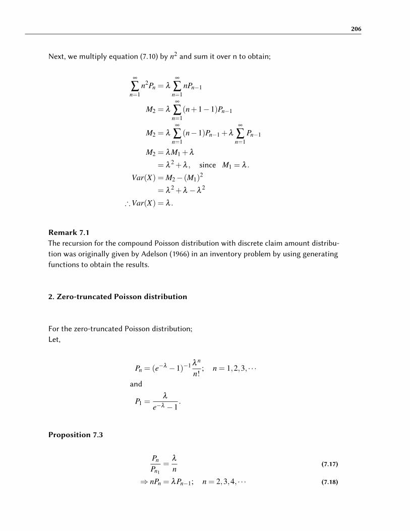
206

Next, we multiply equation (7.10) by n2 and sum it over n to obtain;

∞

∑n=1

n2Pn = λ

∞

∑n=1

nPn−1

M2 = λ

∞

∑n=1

(n+1−1)Pn−1

M2 = λ

∞

∑n=1

(n−1)Pn−1 +λ

∞

∑n=1

Pn−1

M2 = λM1 +λ

= λ2 +λ , since M1 = λ .

Var(X) = M2− (M1)2

= λ2 +λ −λ

2

∴Var(X) = λ .

Remark 7.1The recursion for the compound Poisson distribution with discrete claim amount distribu-tion was originally given by Adelson (1966) in an inventory problem by using generatingfunctions to obtain the results.

2. Zero-truncated Poisson distribution

For the zero-truncated Poisson distribution;Let,

Pn = (e−λ −1)−1 λ n

n!; n = 1,2,3, · · ·

and

P1 =λ

e−λ −1.

Proposition 7.3

Pn

Pn1

=λ

n(7.17)

⇒ nPn = λPn−1; n = 2,3,4, · · · (7.18)

207


P1 = λP0

∴ P1 =λ 1

1!P0.


2P2 = λP1

P2 =λ 2

2P0

∴ P2 =λ 2

2!P0.


3P3 = λP2

⇒ P3 =λ 3

1.2.3P0

∴ P3 =λ 3

3!P0.

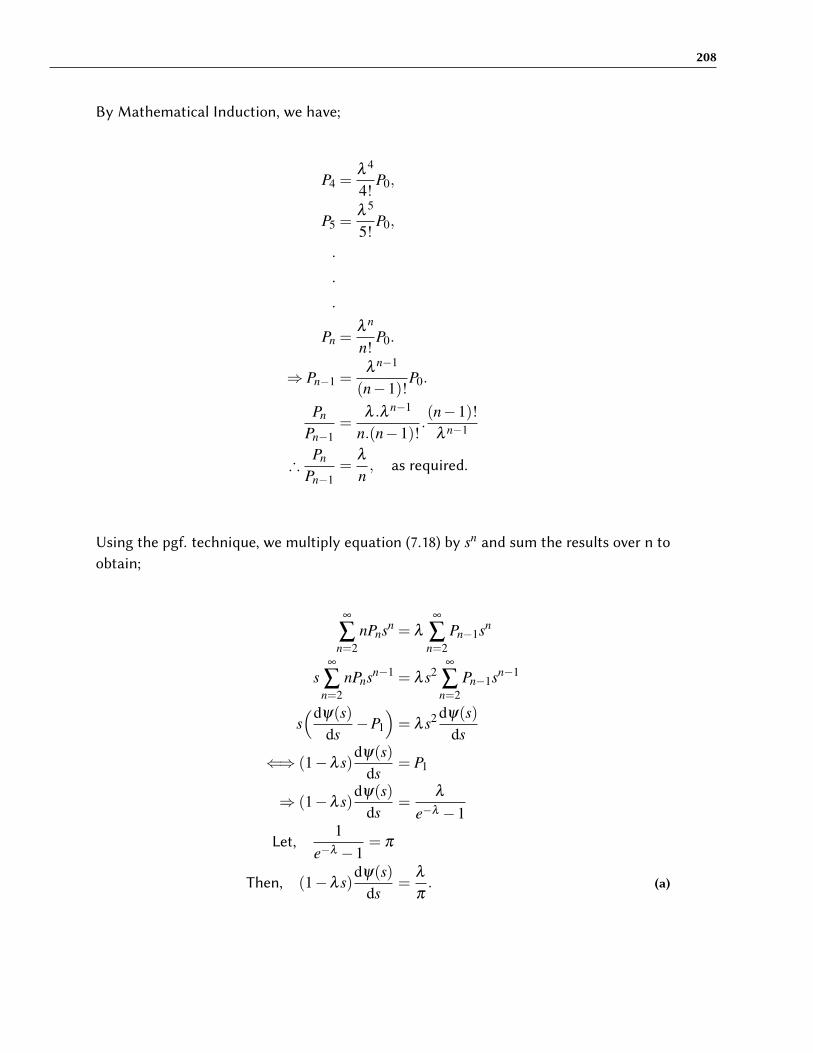
208


P4 =λ 4

4!P0,

P5 =λ 5

5!P0,

.

.

.

Pn =λ n

n!P0.

⇒ Pn−1 =λ n−1

(n−1)!P0.

Pn

Pn−1=

λ .λ n−1

n.(n−1)!.(n−1)!

λ n−1

∴Pn

Pn−1=

λ

n, as required.

Using the pgf. technique, we multiply equation (7.18) by sn and sum the results over n toobtain;

∞

∑n=2

nPnsn = λ

∞

∑n=2

Pn−1sn

s∞

∑n=2

nPnsn−1 = λ s2∞

∑n=2

Pn−1sn−1

s(dψ(s)

ds−P1

)= λ s2 dψ(s)

ds

⇐⇒ (1−λ s)dψ(s)

ds= P1

⇒ (1−λ s)dψ(s)

ds=

λ

e−λ −1

Let,1

e−λ −1= π

Then, (1−λ s)dψ(s)

ds=

λ

π. (a)

209

Integrating both side of (a) above with respect to s, we have;

∫dψ(s) = π

∫λ

1−λ sds

ψ(s) =− ln(1−λ s)

π+ c

Pu�ing s=1;

ψ(1) = 1 =− ln(1−λ )

π+ c1

⇒ c1 = 1− − ln(1−λ )

π

∴ ψ(s) =− ln(1−λ s)

π+− ln(1−λ )

π+1

ψ′(s) =

dψ(s)ds

=λ

(1−λ s)π

ψ′′(s) =

dψ ′(s)ds

=λ 2

(1−λ s)2π

E(X) = ψ′(1)

∴ E(x) =λ

(1−λ )π.

Var(X) = ψ′′(1)+ψ

′(1)− [ψ

′(1)]2

=λ 2

(1−λ )2π+

λ

(1−λ )π− [

λ

(1−λ )π]2

=λ 2

(1−λ )2π+

λ

(1−λ )π− λ 2

(1−λ )2π2

=λ 2π +λπ(1−λ )−1

(1−λ )2π2

=λ 2π +λπ−λ 2π−1

(1−λ )2π2

∴Var(X) =λπ−1

(1−λ )2π2 .

210

Using Feller’s Method, we sum equation (7.18) over n to obtain;

∞

∑n=2

nPn = λ

∞

∑n=2

Pn−1

M1−P1 = λ

⇒M1 = λ +P1

E(X) = M1

∴ E(X) = λ +λ

e−λ −1

∴ E(X) = λ +λ

π

∴ E(X) =λ (π +1)

π.

Next, we multiply (7.18) by n and sum the results over n to obtain;

∞

∑n=2

n2Pn = λ

∞

∑n=2

nPn−1

∞

∑n=2

n2Pn = λ

∞

∑n=2

(n−1+1)Pn−1

M2−P1 = λ

∞

∑n=2

(n−1)Pn−1−∞

∑n=2

Pn−1

M2−P1 = λM1 +λ

M2 = λM1 +λ +P1

⇒M2 = λ2 +

λ 2

π+λ +

λ

π

Var(X) = M2− [M1]2

= λ2 +

λ 2

π+λ +

λ

π−λ

2− λ 2

π2

=λ 2

π+λ +

λ

π− λ 2

π2

∴Var(X) = λ +λ 2

π+

λ

π− λ 2

π2 .

7.3.3 Case (iii) When ξ 6= 0 and λ = 0

211

From equation (7.18), we have;

(1−ξ s)dψ(s)

ds= ξ ψ(s)

⇐⇒ 1ψ(s)

dψ(s)ds

=ξ

1−ξ s

⇒ dsd

logψ(s) =ξ

1−ξ s

Taking the integral on both sides, we have;

∫logψ(s) =

∫ξ ds

1−ξ s

logψ(s) =∫

ξ ds1−ξ s

logψ(s) =− logc(1−ξ s)

⇒ ψ(s) =c1

1−ξ sPu�ing s=1;

⇒ ψ(1) = 1 =c1

1−ξ

∴ c1 = 1−ξ .

∴ ψ(s) =1−ξ

1−ξ s. (7.19)

Suppose we let ξ = p, then we have;

⇒ ψ(s) =1− p1− ps

.

Which is a pgf. of a geometric distribution with parameter 1−ξ .


ψ(s) =(1−ξ s)−1

(1−ξ )−1 .

212

The probability generating function in hypergeometric term is given by;

φ(z) = 1F1(1;1;ξ z)

1F1(1;1;ξ ).

φ′(z) =

1.ξ1

1F1(2;2;ξ z)

1F1(1;1;ξ )

φ′′(z) =

2ξ 2

21F1(3;3;ξ z)

1F1(1;1;ξ )

Let, Λκ =1F1(1+κ;1+κ;ξ )

1F1(1;1;ξ ), κ = 1,2.

E(X) = φ′(1)

∴ E(X) = ξ Λ1.

Var(X) = φ′′+φ

′(1)− [φ

′(1)]2

= ξ2Λ2 +ξ Λ1−ξ

2Λ

21

∴Var(X) = ξ Λ1 +ξ2{Λ2−Λ

21}.

Therefore,

Pn = ξn(1−ξ ); n = 0,1,2,3, · · ·

i.e. Pn = pnq; n = 0,1,2,3, · · ·were, q = 1− p.

3. Geometric DistributionGeometric distribution is given as;

Pn = pnq, n = 0,1,2, · · · ; q = 1− p.

and

P0 = q.

Then, Pn−1 = pn−1q, n = 1,2,3, · · ·

213

Proposition 7.4

Pn

Pn−1=

pnqpn−1q

= p. (7.20)

⇐⇒ Pn = pPn−1, n = 1,2,3, · · · (7.21)


P1 = pP0

∴ P1 = pP0.


P2 = pP1

⇒ P2 = p.pP0

∴ P2 = p2P0.


P3 = pP2

⇒ P3 = p.p2P0

∴ P3 = p3P0.

∴ P4 = p4P0,

∴ P5 = p5P0,

.

.

.

∴ Pn = pnP0.

214

Therefore,

Pn−1 = pn−1P0.

⇒ Pn

Pn−1=

p.pn−1

pn−1

∴Pn

Pn−1= p, as required.

Multiplying both sides of equation (7.21) by sn and sum the results over n, we have;

∞

∑n=1

Pnsn = p∞

∑n=1

Pn−1sn

⇐⇒ ψ(s)−P0 = psψ(s)

⇒ (1− ps)ψ(s) = P0 = q

∴ ψ(s) =q

1− ps.

ψ′(s) =

dψ(s)ds

=qp

(1− ps)2

ψ′′(s) =

dψ′(s)

ds=

2qp2

(1− ps)3

E(X) = ψ′(1)

=qp

(1− p)2

=qpq2

∴ E(X) =pq. Since q = 1− p

ψ′′(1) =

2qp2

(1− p)3

=2p2

q2

Var(X) = ψ′′(1)+ψ

′(1)− [ψ

′(1)]2

=2p2

q2 +pq− p2

q2

∴Var(X) =pq2 . Since p+q = 1

215

Using Feller’s Method, we sum equation (7.21) over n to get;

∞

∑n=1

nPn = p∞

∑n=1

nPn−1

M1 = p( ∞

∑n=1

(n−1)Pn−1 +∞

∑n=1

Pn−1

)M1 = pM1 + p

(1− p)M1 = p

qM1 = p

∴ M1 =pq.

E(X) = M1

∴ E(X) =pq.

Next, we multiply both sides of (7.21) by n2 and sum it over to obtain;

∞

∑n=1

n2Pn = p∞

∑n=1

n2Pn−1

∞

∑n=1

n2Pn = p∞

∑n=1

(n−1+1)2Pn−1

M2 = p∞

∑n=1

[(n−1)2 +2(n−1)+1]Pn−1

M2 = p∞

∑n=1

(n−1)2Pn−1 +2p∞

∑n=1

Pn−1 + p∞

∑n=1

Pn−1

M1 = 2pM2 + p

But, M1 =pq

⇒ (1− p)M2 = 2ppq+ p

M2 =2p2 +qp

q2 .

216

Therefore,

Var(X) = M2− [M1]2

=2p2 +qp

q2 − p2

q2

=2p2 +qp− p2

q2

=p2 +qp

q2

=p(p+q)

q2


Support we assume that;

Pn = pn−1q; n = 1,2,3, · · · ; q = 1− p

and

P1 = q.

Then, Pn−1 = pn−2q; n = 2,3, · · ·

Thus,Pn

Pn−1=

p.pn−2qpn−2q

= p.

⇒ Pn = pPn−1, for n = 2,3, · · · (7.22)


∞

∑n=2

Pnsn = p∞

∑n=2

Pn−1sn

∞

∑n=2

Pnsn = ps∞

∑n=2

Pn−1sn−1

ψ(s)−P1s−P0 = ps(ψ(s)−P0)

But, P1 = q and P0 = 0

217

⇒ (1− ps)ψ(s) = sP1

⇒ (1− ps)ψ(s) = qs

∴ ψ(s) =qs

1− ps.

ψ′(s) =

dψ(s)ds

=qp

(1− ps)2

ψ′′(s) =

dψ ′(s)ds

=2qp2

(1− ps)3

E(X) = ψ′(1)

=qp

(1− p)2

=qpq2

∴ E(X) =pq. Since 1− p = q.

ψ′′(1) =

2qp2

(1− p)3

=2p2

q2

Var(X) = ψ′′(1)+ψ

′(1)− [ψ

′(1)]2

=2p2

q2 +pq− p2

q2

=p2

q2 +pq

=(p2 + pq)

q2

=p(p+q)

q2


Using Feller’s Method, we multiply equation (7.22) by n and sum the results over n toobtain;

∞

∑n=1

nPn = p∞

∑n=1

nPn−1

∞

∑n=1

nPn = p∞

∑n=1

(n+1−1)Pn−1

218

⇒M1 = p[ ∞

∑n=1

(n−1)Pn−1 +∞

∑n=1

Pn−1

]M1 = pM1 + p

(1− p)M1 = p

M1 =p

1− p

⇒M1 =pq

E(X) = M1

∴ E(X) =pq.

Next, we multiply (7.22) by n2 and sum the results over n to obtain;

∞

∑n=1

n2Pn = p∞

∑n=1

n2Pn−1

M2 = p∞

∑n=1

(n−1+1)2Pn−1

M2 = p[ ∞

∑n=1

(n−1)2Pn−1 +2∞

∑n=1

(n−1)Pn−1 +∞

∑n=1

Pn−1

]M2 = p

∞

∑n=1

(n−1)2Pn−1 +2p∞

∑n=1

(n−1)Pn−1 + p∞

∑n=1

Pn−1

M2 = pM2 +2pM1 + p

But, M1 =pq

⇒ (1− p)M2 =2p2

q+ p

M2 =2p2 +qp

q2 .

219

Var(X) = M2− [M1]2

=2p2 +qp

q2 − p2

q2

=2p2 +qp− p2

q2

=p2 +qp

q2

=p(p+q)

q2


4. Truncated Geometric Distribution

For a truncated geometric distribution;

Pn = pn=τq; n = τ,τ +1,τ +2, · · · ; q = 1− p

Pτ = q.

Thus, Pn−1 = p(n−1)−τq; n = τ +1,τ +2, · · ·

Therefore,Pn

Pn−1=

pn−τqp(n−1)−τq

= p (7.23)

⇒ Pn = pPn−1; n = τ +1,τ +2, · · · (7.24)

Using probability generating function technique, we multiply both sides of equation (7.24)by sn and sum the results over n to obtain;

∞

∑n=τ+1

Pnsn = p ∑n=τ+1

Pn−1sn

∞

∑n=τ+1

Pnsn = ps ∑n=τ+1

Pn−1sn−1

ψ(s)−Pτsτ = psψ(s)

But, Pτ = q

220

Therefore;

ψ(s) =qsτ

1− ps.

ψ′(s) =

dψ(s)ds

=τqsτ−1

(1− ps)+

qpsτ

(1− ps)2

ψ′′(s) =

dψ′(s)

ds=

τ(τ−1)qsτ−1

(1− ps)+

2qpτsτ−1

(1− ps)2 +2qp2τsτ

(1− ps)3

E(X) = ψ′(1)

=τq

(1− p)+

qp(1− p)2

=τq2 +qp

q2

=q(τ + p)

q2

∴ E(X) = τ +pq.

ψ′′(1) =

τ(τ−1)q(1− p)

+2qpτ

(1− p)2 +2qp2τ

(1− p)3

But, q = 1− p

Var(X) = ψ′′(1)+ψ

′(1)− [ψ

′(1)]2

= τ(τ−1)+2pτ

q+

2p2

q2 + τ +pq− (τ +

pq)2

= τ2− τ +

2pτ

q+

2p2

q2 + τ +pq− τ

2− 2pτ

q− p2

q2

=2p2

q2 +pq− p2

q2

=p2 + pq

q2

=p(p+q)

q2


Using Feller’s Method, we multiply equation (7.24) by n and sum the results over n toobtain;

221

∞

∑n=τ+1

nPn =∞

∑n=τ+1

nPn−1

∞

∑n=τ+1

nPn =∞

∑n=τ+1

[(n−1)+1]Pn−1

M1− τPτ = p∞

∑n=τ+1

(n−1)Pn−1 + p∞

∑n=τ+1

Pn−1

Pτ = pM1 + p

But, Pτ = q

⇒M1− τq = pM1 + p

(1− p)M1 = p+ τq

qM1 = p+ τq

M1 =p+ τq

qE(X) = M1

∴ E(X) = τ +pq.

Next, we multiply equation (7.24) by n2 and sum the results over n to obtain;

∞

∑n=τ+1

n2Pn = p∞

∑n=τ+1

n2Pn−1

∞

∑n=τ+1

n2Pn = p∞

∑n=τ+1

[(n−1)+1]2Pn−1

M2− τ2Pτ = p

∞

∑n=τ+1

[(n−1)2 +2(n−1)+1]Pn−1

M2− τ2Pτ = p

∞

∑n=τ+1

(n−1)2Pn−1 +2p ∑n=τ+1

(n−1)Pn−1 + p∞

∑n=τ+1

Pn−1

M2− τ2Pτ = pM2 +2pM1 + p

But, Pτ = q and M1 = τ +pq

M2− τ2q = pM2 +2pτ +

2p2

q+ p

(1− p)M2 = τq +2τ p+

2p2

q+ p

222

∴ M2 = τ2 +

2τ pq

+2p2

q2 +pq.

Var(X) = M2− [M1]2

= τ2 +

2τ pq

+2p2

q2 +pq− (τ +

pq)2

= τ2 +

2τ pq

+2p2

q2 +pq− τ

2− 2τ pq− p2

q2

=p2

q2 +pq

=p2 + pq

q2

=p(p+q)

q2


7.3.4 Case (iv) When ξ 6= 0 and λ 6= 0


(1−ξ s)dψ(s)

ds= (ξ −λ )ψ(s)

Assuming that ξ +λ > 0;

Then,

1ψ(s)

dψ(s)ds

=ξ +λ

1−ξ s∫dlogψ(s) = (ξ +λ )

∫ ds1−ξ s

logψ(s) =ξ +λ

−ξlogc(1−ξ s)

logψ(s) =−α logc(1−ξ s)

where, α =ξ +λ

ξ.

⇒ ψ(s) = c1(1−ξ s)−α

223

Pu�ing s=1, we have;

ψ(1) = 1 = c1(1−ξ )−α

⇒ c1 = (1−ξ )α

∴ ψ(s) =( 1−ξ

1−ξ s

)α

. (*)

If α is a positive integer;Then;

ψ(s) = (1−ξ )α(1−ξ )−α

= (1−ξ )α∞

∑n=0

−α

n

(−ξ s)n

= (1−ξ )α∞

∑n=0

(−1)n

−α

n

ξnsn

= (1−ξ )α∞

∑n=0

α +n−1

n

ξnsn.

Therefore;

Pn =

α +n−1

n

ξn(1−ξ )α for 0 < ξ < 1, α > 0

Let, ξ = p

⇒ Pn =

α +n−1

n

pn(1− p)α for 0 < p < 1, α > 0; n = 0,1,2, · · ·

(7.25)

Which is a Negative Binomial Distribution.Its probability generating function in hypergeometric terms is given by;

φ(z) = 2F1(α, [;[;ξ z)

2F1(α, [;[;ξ ).

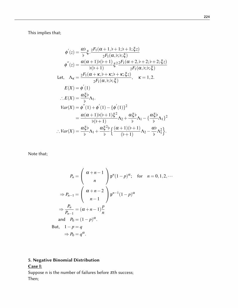
224

This implies that;

φ′(z) =

α[

[ξ .

2F1(α +1, [+1;[+1;ξ z)

2F1(α, [;[;ξ )

φ′′(z) =

α(α +1)[([+1)[([+1)

ξ2 2F1(α +2, [+2;[+2;ξ z)

2F1(α, [;[;ξ )

Let, Λκ =2F1(α +κ, [+κ;[+κ;ξ z)

2F1(α, [;[;ξ ), κ = 1,2.

E(X) = φ′(1)

∴ E(X) =αξ [

[Λ1.

Var(X) = φ′′(1)+φ

′(1)−{φ

′(1)}2

=α(α +1)[([+1)ξ 2

[([+1)Λ2 +

αξ [

[Λ1−{

αξ [

[Λ1}2

∴Var(X) =αξ [

[Λ1 +

αξ 2[

[

{(α +1)([+1)([+1)

Λ2−α[

[Λ

21

}.

Note that;

Pn =

α +n−1

n

pn(1− p)α ; for n = 0,1,2, · · ·

⇒ Pn−1 =

α +n−2

n−1

pn−1(1− p)α

⇒ Pn

Pn−1= (α +n−1)

pn

and P0 = (1− p)α .

But, 1− p = q

⇒ P0 = qα .

5. Negative Binomial DistributionCase I:Suppose n is the number of failures before πth success;Then;

225

Pn =

n+π−1

π−1

pnqπ ; n = 0,1,2, · · · ; q = 1− p

P0 = qπ .

⇒ Pn−1 =

(n−1)+π−1

π−1

pn−1qπ ; n = 0,1,2, · · ·


Pn

Pn−1= (n+π−1)

pn

⇒ nPn = p(n+π−1)Pn−1; n = 1,2,3, · · · (7.26)


P1 = pπP0

∴ P1 = pπP0.


2P2 = p(π +1)P1

⇒ 2P2 = p(π +1)pπP0

∴ P2 =π(π +1)p2

2!P0.


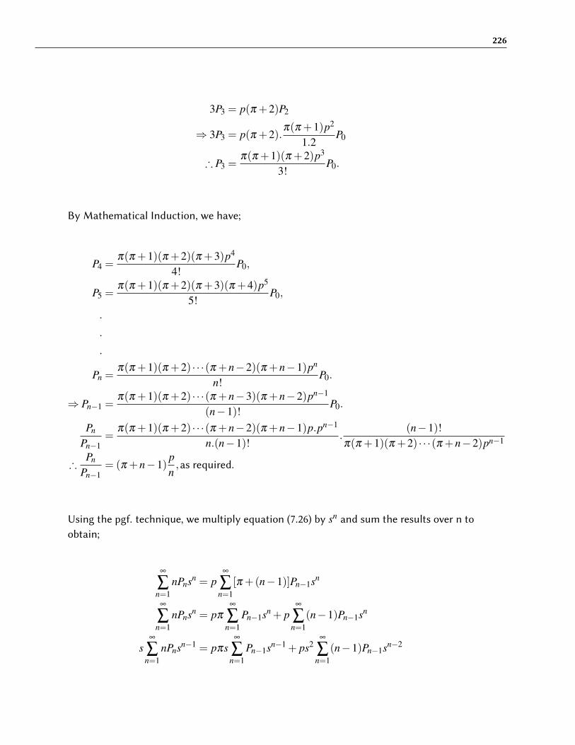
226

3P3 = p(π +2)P2

⇒ 3P3 = p(π +2).π(π +1)p2

1.2P0

∴ P3 =π(π +1)(π +2)p3

3!P0.


P4 =π(π +1)(π +2)(π +3)p4

4!P0,

P5 =π(π +1)(π +2)(π +3)(π +4)p5

5!P0,

.

.

.

Pn =π(π +1)(π +2) · · ·(π +n−2)(π +n−1)pn

n!P0.

⇒ Pn−1 =π(π +1)(π +2) · · ·(π +n−3)(π +n−2)pn−1

(n−1)!P0.

Pn

Pn−1=

π(π +1)(π +2) · · ·(π +n−2)(π +n−1)p.pn−1

n.(n−1)!.

(n−1)!π(π +1)(π +2) · · ·(π +n−2)pn−1

∴Pn

Pn−1= (π +n−1)

pn,as required.


∞

∑n=1

nPnsn = p∞

∑n=1

[π +(n−1)]Pn−1sn

∞

∑n=1

nPnsn = pπ

∞

∑n=1

Pn−1sn + p∞

∑n=1

(n−1)Pn−1sn

s∞

∑n=1

nPnsn−1 = pπs∞

∑n=1

Pn−1sn−1 + ps2∞

∑n=1

(n−1)Pn−1sn−2

227

Thus;

sdψ(s)

ds= pπsψ(s)+ ps2 dψ(s)

ds

⇐⇒ (1− ps)dψ(s)

ds= pπψ(s)

⇒ 1ψ(s)

dψ(s) =pπ

1− psds


∫ dψ(s)ψ(s)

=∫ pπds

(1− ps)

lnψ(s) =−π ln(1− ps)+ lnc

⇒ ψ(s) = c1(1− ps)−π

Pu�ing s=1;

ψ(1) = 1 = c1(1− p)−π

⇒ c1 = qπ .

⇒ ψ(s) = qπ(1− ps)−π

∴ ψ(s) =( q

1− ps

)π

.

ψ′(s) =

pπqπ

(1− ps)π+1

ψ′′(s) =

p2π(π +1)qπ

(1− ps)π+2

=p2π2qπ + p2πqπ

(1− ps)π+2

E(X) = ψ′(1)

=pπqπ

qπ+1

∴ E(X) =pπ

q.

228

and,

ψ′′(1) =

p2π2qπ + p2πqπ

qπ+2

=p2π2 + p2π

q2

Var(X) = ψ′′(1)+ψ

′(1)− [ψ

′(1)]2

=p2π2 + p2π

q2 +pπ

q− [

pπ

q]2

=p2π2 + p2π

q2 +pπ

q− p2π2

q2

=p2π

q2 +pπ

q

=p2π +qpπ

q2

=pπ(p+q)

q2

∴Var(X) =pπ

q2 . Since p+q = 1

Using Feller’s method, we sum equation (7.26) over n, to get;

∞

∑n=1

nPn = p∞

∑n=1

(n+π−1)Pn−1

∞

∑n=1

nPn = p∞

∑n=1

[(n−1)+π]Pn−1

M1 = p∞

∑n=1

(n−1)Pn−1 + pπ

∞

∑n=1

Pn−1

M1 = pM1 + pπ

(1− p)M1 = pπ

M1 =pπ

q. Since 1− p = q

E(X) = M1

∴ E(X) =pπ

q.

229

Next, we multiply equation (7.26) by n and sum the results over n to get;

∞

∑n=1

n2Pn = p∞

∑n=1

n(n+π−1)Pn−1

∞

∑n=1

n2Pn = p∞

∑n=1

[(n−1)+1][(n−1)+π]Pn−1

M2 = p∞

∑n=1

(n−1)2Pn−1 + pπ

∞

∑n=1

(n−1)Pn−1 + p∞

∑n=1

(n−1)Pn−1 + pπ

∞

∑n=1

Pn−1

M2 = pM2 + pπM1 + pM1 + pπ

(1− p)M2 = pπ.pπ

q+ p.

pπ

q+ pπ

qM2 =p2π2

q+

p2π

q+ pπ

⇒M2 =p2π2 + p2π +qpπ

q2

Var(X) = M2− [M1]2

=p2π2 + p2π +qpπ

q2 − p2π2

q2

=p2π + pqπ

q2

=pπ(p+q)

q2

∴Var(X) =pπ

q2 . Since p+q = 1

Case II:Suppose n is the number of trials required to achieve the π th success;Then,

Pn =

n−1

π−1

pn−πqπ , n = π,π +1,π +2, · · · ; q = 1− p

and

Pπ = qπ .

Pn−1 =

(n−1)−1

π−1

p(n−1)−πqπ , n = π +1,π +2, · · · .

230

Thus,Proposition 7.6

Pn

Pn−1=

n−1n−π

p (7.27)

⇒ (n−π)Pn = p(n−1)Pn−1; n = π +1,π +2, · · · (7.28)

ProofSolving (7.28) iteratively, we have;When n=π+1;Equation (7.28) becomes;

Pπ+1 = pπPπ

∴ Pπ+1 = pπPπ .

When n=π+2;Equation (7.28) becomes;

2Pπ+2 = p(π +1)Pπ+1

⇒ 2Pπ+2 = p(π +1).pπPπ

∴ Pπ+2 =π(π +1)p2

2!Pπ

When n=π+3;Equation (7.28) becomes;

3Pπ+3 = p(π +2)Pπ+2

⇒ 3Pπ+3 = p(π +2).π(π +1)p2

1.2Pπ

∴ Pπ+3 =π(π +1)(π +2)p3

3!Pπ

231


Pπ+4 =π(π +1)(π +2)(π +3)p4

4!Pπ ,

Pπ+5 =π(π +1)(π +2)(π +3)(π +4)p5

5!Pπ ,

.

.

.

Pn =π(π +1)(π +2) · · ·(π +n−2)(π +n−1)pn

n!Pπ .

⇒ Pn−1 =π(π +1)(π +2) · · ·(π +n−3)(π +n−2)pn−1

(n−1)!Pπ .

Pn

Pn−1=

π(π +1)(π +2) · · ·(π +n−2)(π +n−1)p.pn−1

n.(n−1)!.

(n−1)!π(π +1)(π +2) · · ·(π +n−2)pn−1

∴Pn

Pn−1=

n−1n−π

p. as required

Using the probability generating function technique, we multiply equation (7.28) by sn

and sum the results over n to obtain;

∞

∑n=π+1

nPnsn−π

∞

∑n=π+1

Pnsn = p∞

∑n=π+1

(n−1)Pn−1sn

s∞

∑n=π+1

nPnsn−1−π

∞

∑n=π+1

Pnsn = ps2∞

∑n=π+1

(n−1)Pn−1sn−2

But, Pπ = qπ

s[dψ(s)

ds−πqπsπ−1

]−π

[ψ(s)−qπsπ

]= ps2 dψ(s)

ds

Therefore,

s(1− ps)dψ(s)

ds= πψ(s)

⇐⇒ 1ψ(s)

=πds

s(1− ps)

232

Integrating both sides with respect to s, we have;

∫ dψ(s)ψ(s)

= π

∫ dss(1− ps)

lnψ(s) = π lns−π ln(1− ps)+ lnc

lnψ(s) = π ln[ s

1− ps

]π

+ lnc

Hence,

ψ(s) = c1

[ s1− ps

]π

Pu�ing s=1;

ψ(1) = 1 = c1

[ s1− p

]π

⇒ c1 = (1− p)π = qπ .

ψ(s) = qπ

[ s1− ps

]π

∴ ψ(s) =[ qs

1− ps

]π

.

ψ′(s) =

dψ(s)ds

=πqπsπ−1

(1− ps)π+

pπqπsπ

(1− ps)π+1

ψ′′(s) =

π(π−1)qπsπ−2

(1− ps)π+

2pπ2qπsπ−1

(1− ps)π+1 +p2π(π +1)qπsπ

(1− ps)π+2

Pu�ing s=1;

ψ′(1) =

πqπ

(1− p)π+

pπqπ

(1− p)π+1

= π +pπ

q

233

Therefore,

ψ′(1) =

qπ + pπ

q

=π(q+ p)

q

∴ ψ′(1) =

π

q. Since q+ p = 1

E(X) = ψ′(1)

∴ E(X) =π

q.

ψ′(1) =

π(π−1)qπ

qπ+

2pπ2qπ

qπ+1 +p2π(π +1)qπ

qπ+2

= π(π−1)+2pπ2

q+

p2π(π +1)q2

Var(X) = ψ′′(1)+ψ

′(1)− [ψ

′(1)]2

= π(π−1)+2pπ2

q+

p2π(π +1)q2 +

π

q− π2

q2

=q2π2−q2π +2pqπ2 + p2π2 + p2π +qπ−π2

q2

=π2(q+ p)2−πq2 +π p2 +π p−π2

q2

=π p2 +π p−πq2

q2

∴Var(X) =π pq2 .


∞

∑n=π+1

nPn−π

∞

∑n=π+1

Pn = p∞

∑n=π+1

(n−1)Pn−1

⇐⇒M1−πPπ = pM1 +π−πPπ

But, Pπ = qπ

M1−πqπ = pM1 +π−πqπ

(1− p)M1 = π

⇒M1 =π

q. Since 1− p = q

234

Therefore,

E(X) = M1

∴ E(X) =π

q.

Multiplying equation (7.28) by n and sum the results over n, we get;

∞

∑n=π+1

n2Pn−π

∞

∑n=π+1

nPn = p∞

∑n=π+1

[(n−1)+1](n−1)Pn−1

M2−π2Pπ − [πM1−π

2Pπ ] = p∞

∑n=π+1

(n−1)2Pn−1 + p∞

∑n=π+1

(n−1)Pn−1

M2−πM1 = pM2 + pM1

But M1 =π

q.

⇒ (1− p)M2 =π2

q+

π pq

∴ M2 =π2 +π p

q2 . Since 1− p = q

Var(X) = M2− [M1]2

=π2 +π p

q2 − π2

q2

∴Var(X) =π pq2 .

6. Truncated Negative Binomial DistributionFor a truncated Negative Binomial Distribution;Let,

Pn =qπ

1−qπ

n+π−1

π−1

pnqπ ; n = 1,2,3, · · · ; q = 1− p

and P1 =pπqπ

1−qπ

Pn−1 =qπ

1−qπ

(n−1)+π−1

π−1

p(n−1)qπ ; n = 1,2,3, · · ·

235

Proposition 7.7

Pn

Pn−1=

(n+π−1)pn

(7.29)

⇒ nPn = p(n+π−1)Pn−1; n = 2,3, · · · (7.30)


P1 = pπP0

∴ P1 = pπP0.


2P2 = p(π +1)P1

⇒ 2P2 = p(π +1)pπP0

∴ P2 =π(π +1)p2

2!P0.


3P3 = p(π +2)P2

⇒ 3P3 = p(π +2)π(π +1)p2

1.2P0

∴ P3 =π(π +1)(π +2)p3

3!P0.

236


P4 =π(π +1)(π +2)(π +3)p4

4!P0,

P5 =π(π +1)(π +2)(π +3)(π +4)p5

5!P0,

.

.

.

Pn =π(π +1)(π +2) · · ·(π +n−2)(π +n−1)pn

n!P0.

⇒ Pn−1 =π(π +1)(π +2) · · ·(π +n−2)pn−1

(n−1)!P0.

Pn

Pn−1=

π(π +1)(π +2) · · ·(π +n−2)(π +n−1)p.pn−1

n.(n−1)!.

(n−1)!π(π +1)(π +2) · · ·(π +n−2)pn−1

∴Pn

Pn−1=

p(π +n−1)n

. as required



∞

∑n=2

nPnsn = p∞

∑n=2

(n+π−1)Pn−1sn

s∞

∑n=2

nPnsn−1 = p∞

∑n=2

[(n−1)+π]Pn−1sn

s∞

∑n=2

nPnsn−1 = p∞

∑n=2

(n−1)Pn−1sn + pπ

∞

∑n=2

Pn−1sn

s∞

∑n=2

nPnsn−1 = ps2∞

∑n=2

(n−1)Pn−1sn−1 + psπ

∞

∑n=2

Pn−1sn−1

s[dψ(s)

ds−P1

]= ps2 dψ(s)

ds+ pπs

[ψ(s)−P0

]But, P0 = 0

and P1 =pπqπ

1−qπ

237

Therefore,

s[dψ(s)

ds− pπqπ

1−qπ

]= ps2 dψ(s)

ds+ pπs

[ψ(s)−P0

]s(1− ps)

dψ(s)ds

= pπψ(s)+pπqπ

1−qπ(7.31)

Note that, equation (7.31) cannot be solved explicitly.


∞

∑n=2

nPn = p∞

∑n=2

(n+π−1)Pn−1

∞

∑n=2

nPn = p∞

∑n=2

[(n−1)+π]Pn−1

M1−P1 = p∞

∑n=2

(n−1)Pn−1 + pπ

∞

∑n=2

Pn−1

M1−P1 = pM1 + pπ

But, P1 =pπqπ

1−qπ

⇒M1 =pπ

q+

pπqπ

q(1−qπ)

E(X) = M1

=pπ(1−qπ)+ pπqπ

q(1−qπ)

=pπ[1−qπ +qπ ]

q(1−qπ)

∴ E(X) =pπ

q(1−qπ).

238

Also, multiplying equation (7.30) by n and sum the results over n, we get;

∞

∑n=2

n2Pn = p∞

∑n=2

n(n+π−1)Pn−1

∞

∑n=2

n2Pn = p∞

∑n=2

[(n−1)+1][(n−1)+π]Pn1

M2−P1 = p∞

∑n=2

(n−1)2Pn−1 + pπ

∞

∑n=2

(n−1)Pn−1 + p∞

∑n=2

(n−1)Pn−1 + pπ

∞

∑n=2

Pn−1

M2−P1 = pM2 + pπM1 + pM1 + pπ

(1− p)M2 = (pπ− p)pπ

q(1−qπ)+ pπ +

pπqπ

1−qπ

Since P1 =pπqπ

1−qπ, and M1 =

pπ

q(1−qπ).

⇒ qM2 =p2π2

q(1−qπ)+

p2π

q(1−qπ)+ pπ +

pπqπ

1−qπ

M2 =p2π2

q2(1−qπ)+

p2π

q2(1−qπ)+

pπ

q+

pπqπ

q(1−qπ)

=p2π2 + p2π + pπq− pπqπ + pπqπ+1

q2(1−qπ)

=p2π2 + pπ(p+q)+ pπqπ(−1+q)

q2(1−qπ)

=p2π2 + pπ− pπqπ

q2(1−qπ)

⇒M2 =p2π2 + p2π + pπ

q+

pπqπ

q(1−qπ)

Var(X) = M2−{M1}2

=p2π2 + p2π + pπ

q+

pπqπ

q(1−qπ)−{ pπ

q(1−qπ)}

∴Var(X) =pπ

q2(1−qπ)− p2π2qπ

q2(1−qπ)2 .

From Equation (*) above, we have;

ψ(s) =( 1−ξ

1−ξ s

)α

239

If α is a negative integer;Let α =−ω where, ω is a positive integer,Then,

ψ(s) = (1−ξ )−ω(1−ξ s)ω

= (1−ξ )−ωω

∑n=0

ω

n

(−ξ s)n

⇒ ψ(s) =ω

∑n=0

ω

n

(−ξ s)n

(1−ξ )ω

=ω

∑n=0

ω

n

(−ξ s)n

(1−ξ )n(1−ξ )ω−n

=ω

∑n=0

ω

n

( −ξ

1−ξ

)n( 11−ξ

)ω−nsn

Let, p =−ξ

1−ξ

Thus,

1− p = 1+ξ

1−ξ

=1

1−ξ

∴ ψ(s) =ω

∑n=0

ω

n

pn(1− p)ω−nsn; ξ < 0

Therefore,

Pn =

ω

n

pn(1− p)ω−n, for n = 0,1,2, · · · ,ω.

Which is a Binomial distribution.

Let, Pn =

ω

n

pn(1− p)ω−n, for n = 0,1,2, · · · ,ω; q = 1− p

⇒ Pn−1 =

ω

n−1

pn−1(1− p)ω−(n−1), for n = 1,2, · · · ,ω.

240


Pn

Pn−1=

(ω−n+1)nq

.

⇐⇒ nPn = (ω−n+1)pq

Pn−1; for n = 1,2,3, · · · ,ω (7.32)


P1 =ω pq

P0

∴ P1 =ω pq

P0.


2P2 = (ω−1)pq

P1

⇒ 2P2 = (ω−1)pq

ω pq

P0

∴ P2 =ω(ω−1)

(pq

)2

2!P0.


3P3 = (ω−2)pq

P2

⇒ 3P3 = (ω−2)pq

ω(ω−1)(

pq

)2

1.2P0

∴ P3 =ω(ω−1)(ω−2)

(pq

)3

3!P0.

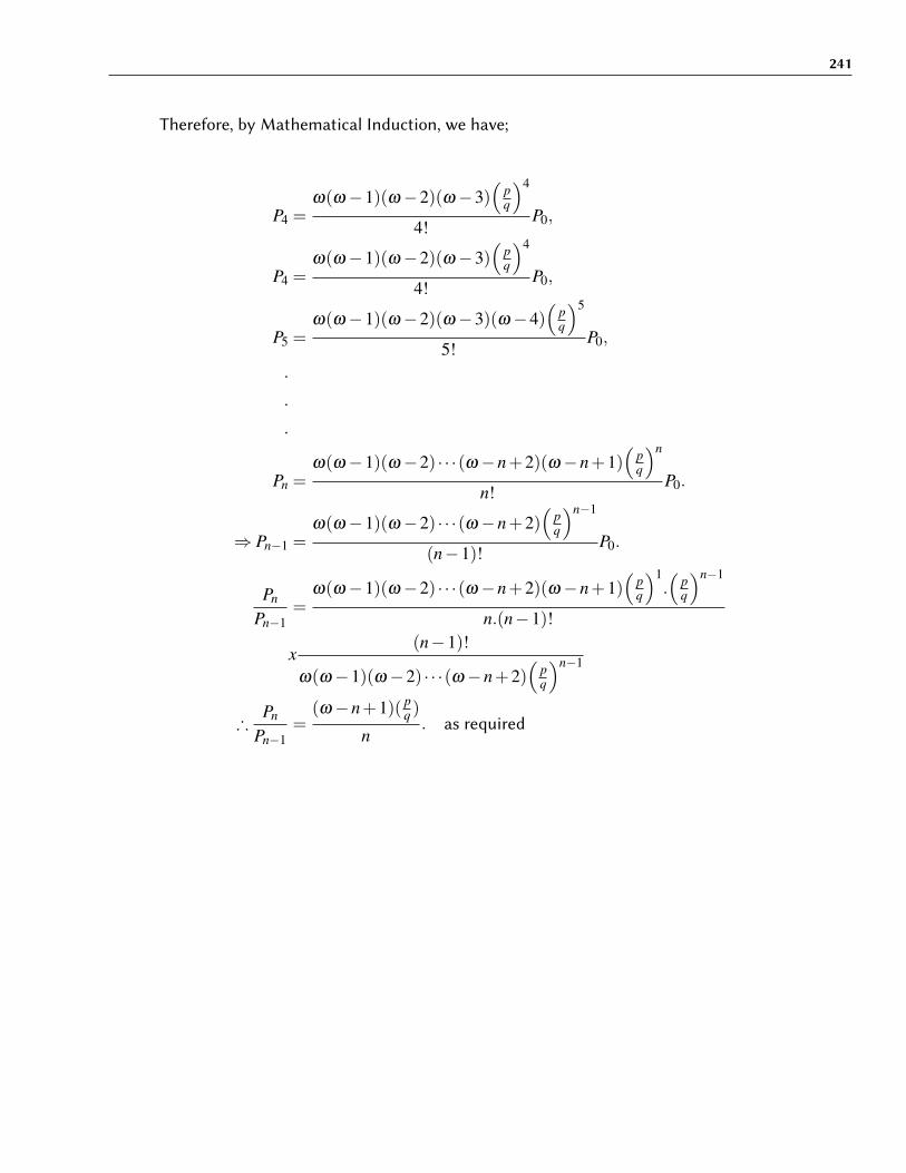
241


P4 =ω(ω−1)(ω−2)(ω−3)

(pq

)4

4!P0,

P4 =ω(ω−1)(ω−2)(ω−3)

(pq

)4

4!P0,

P5 =ω(ω−1)(ω−2)(ω−3)(ω−4)

(pq

)5

5!P0,

.

.

.

Pn =ω(ω−1)(ω−2) · · ·(ω−n+2)(ω−n+1)

(pq

)n

n!P0.

⇒ Pn−1 =ω(ω−1)(ω−2) · · ·(ω−n+2)

(pq

)n−1

(n−1)!P0.

Pn

Pn−1=

ω(ω−1)(ω−2) · · ·(ω−n+2)(ω−n+1)(

pq

)1.(

pq

)n−1

n.(n−1)!

x(n−1)!

ω(ω−1)(ω−2) · · ·(ω−n+2)(

pq

)n−1

∴Pn

Pn−1=

(ω−n+1)( pq )

n. as required

242

Its pgf. in hypergeometric terms is given by;

φ(z) = 2F1(α,1;1;ξ z)

2F1(α,1;1;ξ ).

φ′(z) =

1.αξ

12F1(α +1,2;2;ξ z)

2F1(α,1;1;ξ )

φ′′(z) =

1(2)α(α +1)ξ 2

1(2)2F1(α +2,3;3;ξ z)

2F1(α,1;1;ξ )

Let, Λκ =2F1(α +κ,1+κ;1+κ;ξ )

2F1(α,1;1;ξ ), κ = 1,2.

E(X) = φ′(1)

∴ E(X) = αξ Λ1.

and,

Var(X) = φ′′(1)+φ

′(1)− [φ

′(1)]2

= α(α +1)ξ 2Λ2 +αξ Λ1− [αξ Λ1]

2

∴Var(X) = αξ Λ1 +αξ2{(α +1)Λ2−αΛ

21}.



qω

∑n=1

nPnsn = pω

∑n=1

[ω− (n−1)]Pn−1sn

qs∞

∑n=1

nPn−1sn−1 = ω p∞

∑n=1

Pn−1sn− p∞

∑n=1

(n−1)Pn−1sn

qs∞

∑n=1

nPn−1sn−1 = ω ps∞

∑n=1

Pn−1sn−1− ps2∞

∑n=1

(n−1)Pn−1sn−2

qsdψ(s)

ds= ω psψ(s)− ps2 dψ(s)

ds1

ψ(s)dψ(s) =

ω pq+ ps

ds

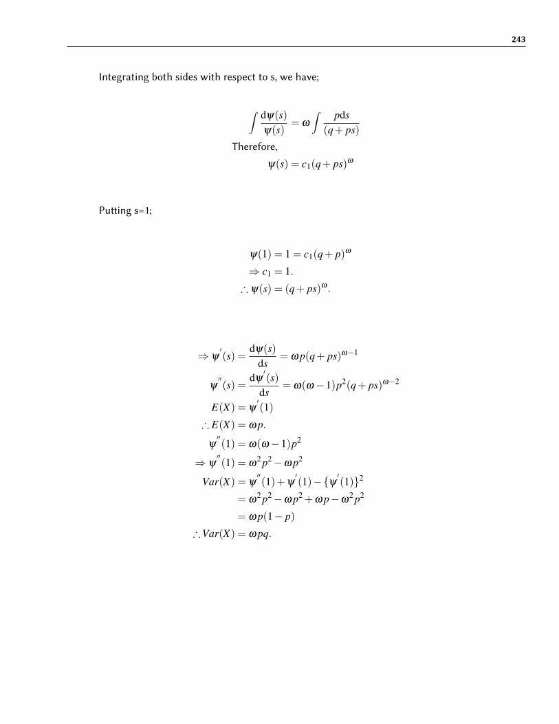
243

Integrating both sides with respect to s, we have;

∫ dψ(s)ψ(s)

= ω

∫ pds(q+ ps)

Therefore,

ψ(s) = c1(q+ ps)ω

Pu�ing s=1;

ψ(1) = 1 = c1(q+ p)ω

⇒ c1 = 1.

∴ ψ(s) = (q+ ps)ω .

⇒ ψ′(s) =

dψ(s)ds

= ω p(q+ ps)ω−1

ψ′′(s) =

dψ′(s)

ds= ω(ω−1)p2(q+ ps)ω−2

E(X) = ψ′(1)

∴ E(X) = ω p.

ψ′′(1) = ω(ω−1)p2

⇒ ψ′′(1) = ω

2 p2−ω p2

Var(X) = ψ′′(1)+ψ

′(1)−{ψ

′(1)}2

= ω2 p2−ω p2 +ω p−ω

2 p2

= ω p(1− p)

∴Var(X) = ω pq.

244


ω

∑n=1

nPn =ω

∑n=1

(ω−n+1)pq

Pn−1

ω

∑n=1

nPn =pq

ω

∑n=1

[ω− (n−1)]Pn−1

M1 =pq

ω

ω

∑n=1

Pn−1−pq

ω

∑n=1

(n−1)Pn−1

M1 =pq[ω(1−Pω)]−

pq[M1−ωPω ]

Therefore,

M1 =pq

ω− pq

M1

⇐⇒ qM1 + pM1 = ω p

(q+ p)M1 = ω p

∴ M1 = ω p. Since q+ p = 1

E(X) = M1

∴ E(X) = ω p.

245

Again, multiplying equation (7.32) by n and sum the results over n, we get;

ω

∑n=1

n2Pn =ω

∑n=1

n(ω−n+1)pq

Pn−1

ω

∑n=1

n2Pn =pq

ω

∑n=1

[(n−1)+1][ω− (n−1)]Pn−1

M2 =pq

[ω

ω

∑n=1

(n−1)Pn−1−ω

∑n=1

(n−1)2Pn−1 +ω

ω

∑n=1

Pn−1−ω

∑n=1

(n−1)Pn−1

]M2 =

pq

[ω(M1−ωPω)− (M2−ω

2Pω)+ω(1−Pω)− (M1−ωPω)]

M2 =pq

[ωM1−M2 +ω−M1

]But, M1 = ω p

⇒M2 =pq

[ω

2 p−M2 +ω−ω p]

⇐⇒ qM2 = ω p2− pM2 +ω p−ω p2

⇒ (q+ p)M2 = ω2 p2 +ω p−ω p2

∴ M2 = ω2 p2 +ω p−ω p2.

Var(X) = M2−{M1}2

= ω2 p2 +ω p−ω p2−ω

2 p2

= ω p(1− p)

∴Var(X) = ω pq.

7.4 Sundt - Jewell (1981) Class

Remark 7.2Sundt, B. and Jewell, W.S.(1981) have shown that: Poisson, Binomial, Negative Binomialand Geometric distributions are the only members of the family of claim number distribu-tions.

7.5 Panjer’s Class of order k

Sundt and Jewell (1981) generalized Panjer’s (1981) recursive algorithm to the class ofcounting distributions with discrete density {Pn}∞

n=0 satisfying the recursion;

246

Pn = (ξ +λ

n)Pn−1; n = π +1,π +2, · · · (7.33)

7.6 Special Cases of Panjer’s Class of Order k

7.6.1 When π = 0, we obtain Panjer’s Class

Pn = (ξ +λ

n)Pn−1; n = 1,2,3, · · ·

and P1 > 0, P0 = 0

nPn = (ξ n+λ )Pn−1

= [ξ (n−1+1)+λ ]Pn−1

∴ nPn = ξ (n−1)Pn−1 +(ξ +λ )Pn−1; n = 1,2,3, · · ·

Proposition 7.9

nPn = (ξ n+λ )Pn−1 (7.34)


P1 = (ξ +λ )P0

⇒ P1 = (ξ +λ )P0

∴ P1 =(ξ +λ )

1!P0.


247

2P2 = (ξ +λ )(2ξ +λ )P0

⇒ P2 =(ξ +λ )(2ξ +λ )

1.2P0

∴ P2 =(ξ +λ )(2ξ +λ )

2!P0.


3P3 = (3ξ +λ )P2

⇒ 3P3 = (3ξ +λ )(ξ +λ )(2ξ +λ )

1.2P0

∴ P3 =(ξ +λ )(2ξ +λ )(3ξ +λ )

3!P0.


P4 =(ξ +λ )(2ξ +λ )(3ξ +λ )(4ξ +λ )

4!P0,

P5 =(ξ +λ )(2ξ +λ )(3ξ +λ )(4ξ +λ )(5ξ +λ )

5!P0,

.

.

.

Pn =(ξ +λ )(2ξ +λ )(3ξ +λ ) · · ·((n−1)ξ +λ )(nξ +λ )

n!P0.

⇒ Pn−1 =(ξ +λ )(2ξ +λ ) · · ·((n−1)ξ +λ )

(n−1)!P0.

Pn

Pn−1=

(ξ +λ )(2ξ +λ ) · · ·((n−1)ξ +λ )(nξ +λ )

n.(n−1)!.

(n−1)!(ξ +λ )(2ξ +λ )(3ξ +λ ) · · ·((n−1)ξ +λ )

∴Pn

Pn−1=

(nξ +λ )

n. as required

248

Multiplying equation (7.34) by sn and summing over n, we obtain;

∞

∑n=1

nPnsn = ξ

∞

∑n=1

(n−1)Pn−1sn +(ξ +λ )∞

∑n=1

Pn−1sn

sdψ(s)

ds= ξ s2

∞

∑n=1

(n−1)Pn−1sn−2 +(ξ +λ )s∞

∑n=1

Pn−1sn−1

dψ(s)ds

= ξ sdψ(s)

ds+(ξ +λ )ψ(s)

(1−ξ s)dψ(s)

ds= (ξ +λ )ψ(s) (7.35)

When ξ 6= 0, λ = 0 and (ξ +λ )≥ 0Then,

(1−ξ s)dψ(s)

ds= (ξ +λ )ψ(s) = P1

When (ξ +λ ) = 0, then ξ 6= 0Thus,

(1−ξ s)dψ(s)

ds= P1

⇒ dψ(s)ds

=P1

1−ξ s

⇒ ψ(s) =∫ P1ds

1−ξ s

=P1

ξ

∫ −ξ ds1−ξ s

=P1

ξlog(1−ξ s)+ c1

249

Pu�ing s=1;

ψ(1) = 1 =P1

ξlog(1−ξ )+ c1

=P1

ξc1 log(1−ξ )

⇒ c1 =ξ

P1 log(1−ξ )

Therefore,

ψ(s) =log(1−ξ s)log(1−ξ )

.

Which is the probability generating function for a logarithmic distribution with parameterξ .

Pn =ξ n

−n log(1−ξ ); for n = 1,2,3, · · · ; 0 < ξ < 1.

Suppose we let p = ξ ;

⇒ Pn =pn

−n logq; for n = 1,2,3, · · · ; q = 1− p.

and P1 =p

logq

Thus,

Pn−1 =pn−1

−(n−1) logq; for n = 2,3,4, · · ·

⇒ Pn

Pn−1=

(n−1)pn

.

⇐⇒ nPn = p(n−1)Pn−1; n = 2,3,4, · · · (7.36)

Solving (7.36) iteratively, we have;When n=1;

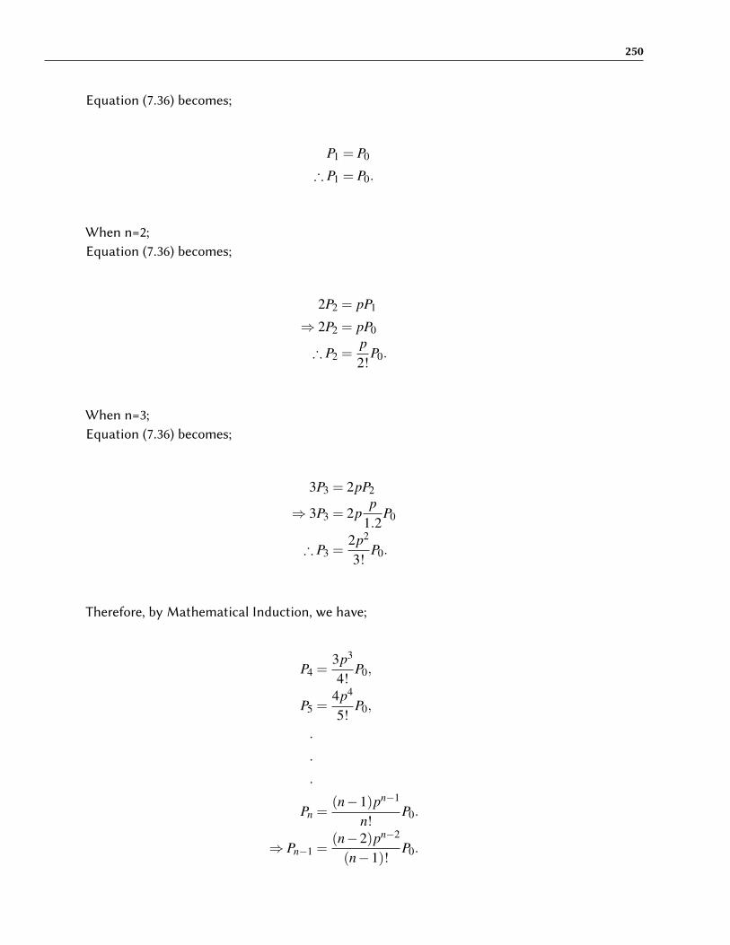
250


P1 = P0

∴ P1 = P0.


2P2 = pP1

⇒ 2P2 = pP0

∴ P2 =p2!

P0.


3P3 = 2pP2

⇒ 3P3 = 2pp

1.2P0

∴ P3 =2p2

3!P0.


P4 =3p3

4!P0,

P5 =4p4

5!P0,

.

.

.

Pn =(n−1)pn−1

n!P0.

⇒ Pn−1 =(n−2)pn−2

(n−1)!P0.

251

Therefore,

Pn

Pn−1=

(n−2).(n−1)p.pn−2

n.(n−1)!.

(n−1)!(n−2)pn−2

∴Pn

Pn−1=

p(n−1)n

. as required



∞

∑n=2

nPnsn = p∞

∑n=2

(n−1)Pn−1sn

s∞

∑n=2

nPnsn−1 = ps2∞

∑n=2

(n−1)Pn−1sn−2

s[dψ(s)

ds−P1

]= ps2 dψ(s)

ds

(1− ps)dψ(s)

ds=−p− logq

; Since P1 =−p

logqTherefore,∫

dψ(s) =1

logq

∫ −pds1− ps

Thus,

ψ(s) =log(1− ps)

logq.

ψ′(s) =

−p(1− ps) logq

ψ′′(s) =

dψ′(s)

ds=

−p2

(1− ps)2 logq

E(X) = ψ′(1)

=−p

(1− p) logq

∴ E(X) =−p

q logq.

ψ′′(1) =

−p2

(1− p)2 logq

=−p2

q2 logq

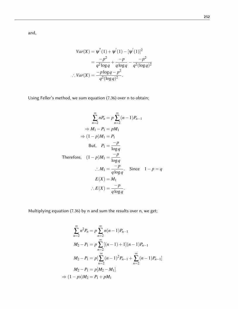
252

and,

Var(X) = ψ′′(1)+ψ

′(1)− [ψ

′(1)]2

=−p2

q2 logq+−p

q logq− −p2

q2(logq)2

∴Var(X) =−p logq− p2

q2(logq)2 .


∞

∑n=2

nPn = p∞

∑n=2

(n−1)Pn−1

⇒M1−P1 = pM1

⇒ (1− p)M1 = P1

But, P1 =−p

logq

Therefore, (1− p)M1 =−p

logq

∴ M1 =−p

q logq. Since 1− p = q

E(X) = M1

∴ E(X) =−p

q logq.

Multiplying equation (7.36) by n and sum the results over n, we get;

∞

∑n=2

n2Pn = p∞

∑n=2

n(n−1)Pn−1

M2−P1 = p∞

∑n=2

[(n−1)+1](n−1)Pn−1

M2−P1 = p[∞

∑n=2

(n−1)2Pn−1 +∞

∑n=2

(n−1)Pn−1]

M2−P1 = p[M2−M1]

⇒ (1− ps)M2 = P1 + pM1

253

But,

M1 =−p

q logqand P1 =

−plogq

⇒ (1− ps)M2 =−p

logq+−p2

q logq

∴ M2 =−p

q logq+−p2

q2 logq.

Var(X) = M2−{M1}2

=−p

q logq+−p2

q2 logq−{ −p

q logq

}2

∴Var(X) =−p logq− p2

q2(logq)2 .

Remark (7.3)

7.6.2 When π = 1, we obtain a Willmot (1988) Class


Pn = (ξ +λ

n)Pn−1; n = 2,3, · · · (**)

Remark (7.4)Schroter (1990) generalized Panjer’s recursive algorithm to the class of counting distribu-tions satisfying the class;

Pn = (ξ +λ

n)Pn−1 +

cn

Pn−2; n = 1,2,3, · · ·

with P−1 = 0 for some constants ξ ,λ and c.

Case I: Let ξ = p and λ =−pFrom (**), we have;

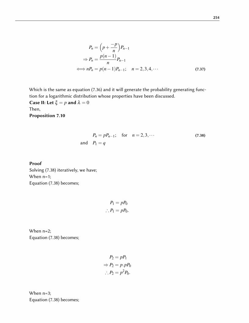
254

Pn =(

p+−pn

)Pn−1

⇒ Pn =p(n−1)

nPn−1

⇐⇒ nPn = p(n−1)Pn−1; n = 2,3,4, · · · (7.37)

Which is the same as equation (7.36) and it will generate the probability generating func-tion for a logarithmic distribution whose properties have been discussed.Case II: Let ξ = p and λ = 0Then,Proposition 7.10

Pn = pPn−1; for n = 2,3, · · · (7.38)

and P1 = q


P1 = pP0

∴ P1 = pP0.


P2 = pP1

⇒ P2 = p.pP0

∴ P2 = p2P0.


255

P3 = pP2

⇒ P3 = p.p2P0

∴ P3 = p3P0.

⇒ P4 = p4P0,

P5 = p5P0,

.

.

.

Pn = pnP0.

⇒ Pn−1 = pn−1P0.

Pn

Pn−1=

p.pn−1

pn−1

∴Pn

Pn−1= p. as required

Which is the probability generating function for Geometric Distribution Type II.

Multiplying equation (7.38) by sn and sum the results over n to obtain;

∞

∑n=2

Pnsn = p∞

∑n=2

Pn−1sn

ψ(s)−P1 = psψ(s)

⇒ (1− ps)ψ(s) = P1

But, P1 = q

∴ ψ(s) =q

1− ps.

ψ′(s) =

dψ(s)ds

=pq

(1− ps)2

ψ′′(s) =

dψ′(s)

ds=

2p2q(1− ps)3

256

Therefore,

E(X) = ψ′(1)

=pq

(1− p)2

=pqq2

∴ E(X) =pq.

Var(X) = ψ′′(1)+ψ

′(1)− [ψ

′(1)]2

=2p2q

(1− p)3 +pq− p2

q2

=2p2 + pq− p2

q2

=p2 + pq

q2

=p(p+q)

q2

∴Var(X) =pq2 .

Its probability generation function in hypergeometric term is given by;

φ(z) = 1F1(1;1; pz)

1F1(1;1; p).

φ′(z) = p.1F1(2;2; pz)

1F1(1;1; p)

φ′′(z) = p2 1F1(3;3; pz)

1F1(1;1; p)

Let, Λκ =1F1(1+κ;1+κ; p)

1F1(1;1; p), κ = 1,2.

E(X) = φ′(1)

∴ E(X) = pΛ1.

Var(X) = φ′′(1)+φ

′(1)−{φ

′(1)}2

= p2Λ2 + pΛ1− p2

Λ21

∴Var(X) = pΛ1 + p2{Λ2−Λ21}.

257

7.7 Panjer’s - Willmot (1982) Class

Consider the counting distributions whose discrete density {Pn}∞n=0 satisfying a class in

the form;

Pn =k

∑ι=1

(ξι +

λι

n

); n = 1,2,3, · · · (7.39)

with Pn = 0 for n < 0.

Therefore,Proposition 7.11

nPn =k

∑ι=1

(nξι +λι)Pn−1 (7.40)

= Pn−1

k

∑ι=1

{ξι(n−1+1)+λι

}∴ nPn = Pn−1

k

∑ι=1

ξι(n−1)+Pn−1

k

∑ι

(ξι +λι); n = 1,2,3, · · · (7.41)


P1 =k

∑ι=1

(ξι +λι)P0

∴ P1 =∑

kι=1(ξι +λι)

1!P0.


258

2P2 =k

∑ι=1

(2ξι +λι)P1

⇒ 2P2 =k

∑ι=1

(2ξι +λι)∑

kι=1(ξι +λι)

1P0

∴ P2 =∑

kι=1(ξι +λι)(2ξι +λι)

2!P0.


3P3 =k

∑ι=1

(3ξι +λι)P2

⇒ 3P3 =k

∑ι=1

(3ξι +λι)∑

kι=1(ξι +λι)(2ξι +λι)

1.2P0

P3 =∑

kι=1(ξι +λι)(2ξι +λι)(3ξι +λι)

3!P0.


P4 =∑

kι=1(ξι +λι)(2ξι +λι)(3ξι +λι)(4ξι +λι)

4!P0,

P5 =∑

kι=1(ξι +λι)(2ξι +λι)(3ξι +λι)(4ξι +λι)(5ξι +λι)

5!P0,

.

.

.

Pn =∑

kι=1(ξι +λι)(2ξι +λι) · · ·((n−1)ξι +λι)(nξι +λι)

n!P0.

⇒ Pn−1 =∑

kι=1(ξι +λι)(2ξι +λι) · · ·((n−1)ξι +λι)

(n−1)!P0.

Pn

Pn−1=

∑kι=1(ξι +λι)(2ξι +λι) · · ·((n−1)ξι +λι)(nξι +λι)

n.(n−1)!.

(n−1)!

∑kι=1(ξι +λι)(2ξι +λι) · · ·((n−1)ξι +λι)

∴Pn

Pn−1=

k

∑ι=1

(nξι +λι)

n. as required

259

Multiplying equation (7.41) by sn and sum the results over n, we obtain;

s∞

∑n=1

nPnsn−1 =k

∑ι=1

ξιs2∞

∑n=1

(n−1)Pn−1sn−2 +k

∑ι=1

(ξι +λι)s∞

∑n=1

Pn−1sn−1

sdψ(s)

ds=

k

∑ι=1

ξιs2∞

∑n=1

(n−1)Pn−1sn−2 +k

∑ι=1

(ξι +λι)s∞

∑n=1

Pn−1sn−1

dψ(s)ds

=k

∑ι=1

ξιsdψ(s)

ds+

k

∑ι=1

(ξι +λι)ψ(s)

Therefore,

(1− sk

∑ι=1

ξι)dψ(s)

ds=

k

∑ι=1

(ξι +λι)ψ(s) (7.42)

7.8 Special Cases of Panjer’s - Willmot (1982) Class and theirProperties

7.8.1 When k=1, we obtain Panjer’s Class

Equation (7.39) becomes Panjer’s Class;

Pn =(

ξ +λ

n

)Pn−1; n = 1,2,3, · · ·

and equation (7.42) becomes;

(1−ξ s

)dψ(s)ds

=(

ξ +λ

)ψ(s).

Which is as discussed in section (7.2) - Panjer’s (1981) class.

7.8.2 When k=2, we obtain the pgf. which does not satisfy existing probabilitydistributions

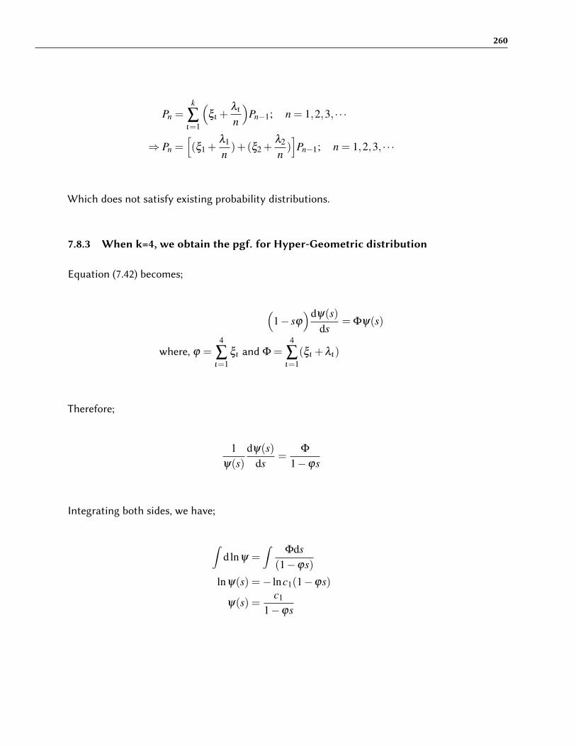
260

Pn =k

∑ι=1

(ξι +

λι

n

)Pn−1; n = 1,2,3, · · ·

⇒ Pn =[(ξ1 +

λ1

n)+(ξ2 +

λ2

n)]Pn−1; n = 1,2,3, · · ·

Which does not satisfy existing probability distributions.

7.8.3 When k=4, we obtain the pgf. for Hyper-Geometric distribution


(1− sϕ

)dψ(s)ds

= Φψ(s)

where, ϕ =4

∑ι=1

ξι and Φ =4

∑ι=1

(ξι +λι)

Therefore;

1ψ(s)

dψ(s)ds

=Φ

1−ϕs


∫dlnψ =

∫Φds

(1−ϕs)

lnψ(s) =− lnc1(1−ϕs)

ψ(s) =c1

1−ϕs

261

Pu�ing s=1;

ψ(1) = 1 =c1

1−ϕ

⇒ c1 = 1−ϕ

∴ ψ(s) =1−ϕ

1−ϕs.

Which is the probability generating function for a hypergeometric distribution with pa-rameter 1−ϕ.

The pgf. in hypergeometric term is given by;

φ(z) = 1F1(1;1;ϕz)

1F1(1;1;ϕ).

φ′(z) =

1.ϕ1

1F1(2;2;ϕz)

1F1(1;1;ϕ)

φ′′(z) =

2ϕ2

21F1(3;3;ϕz)

1F1(1;1;ϕ)

Let, Λκ =1F1(1+κ;1+κ;ϕ)

1F1(1;1;ϕ), κ = 1,2.

E(X) = φ′(1)

∴ E(X) = ϕΛ1.

Var(X) = φ′′+φ

′(1)− [φ

′(1)]2

= ϕ2Λ2 +ϕΛ1−ϕ

2Λ

21

∴Var(X) = ϕΛ1 +ϕ2{Λ2−Λ

21}.

8 KAPUR’S RECURSIVE MODEL IN BIRTH ANDDEATH PROCESSES AT EQUILIBRIUM

8.1 Introduction

In this chapter, we study the generalized cases of birth and death processes in its steadystate using di�erence di�erential equations.Expression for the probability distributions, probability generating function, and momentsin terms of hypergeometric functions are derived.The relations between hypergeometric functions will be used to give their interpretationin terms of probability of extintions for these generalized birth and death processes.

8.2 Kapur’s generalized birth and death processes

Kapur’s generalized birth and death processes can be expressed as a ratio of polynomialsPι and Pι−1 in ι , such that the equilibrium solution is given by;

Pι

Pι−1=

λι−1

µι

, µι 6= 0 (8.1)

which can be re-wri�en as;

Pι

Pι−1=

(ι +a1−1)(ι +a2−1) · · ·(ι +ap−1)ρ(ι +b1−1)(ι +b2−1) · · ·(ι +bq−1)

. (8.2)

Hence, the pgf. in hypergeometric terms is expressed as;

φ(z) = p+1Fq(1,a1, · · · ,ap;b1, · · · ,bq;ρz)

p+1Fq(1,a1, · · · ,ap;b1, · · · ,bq;ρ).

Let a1, · · · ,ap = aι for ι=1,2,3,· · · ,p and b1, · · · ,bq = bτ for τ=1,2,3,· · · ,q.Therefore;

φ(z) = p+1Fq(1,aι ;bτ ;ρz)

p+1Fq(1,aι ;bτ ;ρ).

264

This implies that;

φ′(z) =

1

p+1Fq(1,aι ;bτ ;ρ)

ddz{p+1Fq(1,aι ;bτ ;ρz)}

=1


aιρ

bτ

.p+1Fq(1,aι +1;bτ +1;ρz)

=aιρ

bτ

p+1Fq(2,aι +1;bτ +1;ρz)


φ′′(z) =

1


ddz{p+1Fq(2,aι +1;bτ +1;ρz)}

=1


aι(aι +1)ρ2

bτ(bτ +1){p+1Fq(2+1,aι +2;bτ +2;ρz)}

=aι(aι +1)ρ2

bτ(bτ +1)p+1Fq(3,aι +2;bτ +2;ρz)


Let, Λκ =p+1Fq(1+κ,aι +κ;bτ +κ;ρ)

p+1Fq(1,aι ;bτ ;ρ); κ = 1,2.

E(X) = φ′(1)

∴ E(X) =aι

bτ

ρΛ1.

and

Var(X) = φ′′(1)+φ

′(1)− [φ

′(1)]2

=aι(aι +1)ρ2

bτ(bτ +1)Λ2 +

aι

bτ

ρΛ1−a2

ι

b2τ

ρ2Λ

21

∴Var(X) =aι

bτρΛ1 +

aιρ2

bτ

[aι +1bτ +1

Λ2−aι

bτ

Λ21

].

Moments generating function

The moment generating function is given by;

ϕ(θ) =ρ

∑ι=0

Pιeιθ

∴ ϕ(θ) =p=1Fq(1,aι ;bτ ;ρeθ )

p=1Fq(1,aι ;bτ ;ρ).

Which, on replacing eθ by z, yields the probability generating function φ(lnz).The factorial moment of order δ is given by;

265

µ′δ=

ρ

∑ι=δ

ι(ι−1)(ι−2) · · ·(ι−δ +1)Pι

=ρ

∑ι=0

(ι +δ )!ι

Pι+δ

∴ µ′δ= δ !

(aι)δ

(bτ)δ

ρδ .

p+1Fq(1+δ ,aι +δ ;bτ +δ ;ρ)

p+1Fq(1,aι ;bτ ;ρ); ι = 1,2,3, · · · , p; τ = 1,2,3, · · · ,q.

8.3 Special Cases of Kapur (1978 a) generalized birth and deathprocesses

8.3.1 Case 1: λι = (ιa1 +b1) , µι = (ιc1 +d1)

For λι = (ιa1 +b1) , µι = (ιc1 +d1), the basic di�erence di�erential equations at equi-librium are:

0 = (c1 +d1)P1−b1P0 (8.3)

and

0 = ((ι +1)c1 +d1)Pι+1 +((ι−1)a1 +b1)Pι−1−{(ιa1 +b1)+(ιc1 +d1)}Pι ; ι ≥ 1(8.4)


Pι

Pι−1=

(ι−1)a1 +b1

ιc1 +d1; ι ≥ 1 (8.5)


266

(c1 +d1)P1 = b1P0

⇒ P1 =b1

c1 +d1P0

∴ P1 =b1

c1 +d1P0. (8.6)

Solving (8.4) iteratively, we have;When ι=1;Equation (8.4) becomes;

0 = (2c1 +d1)P2−{(a1 +b1)+(c1 +d1)}P1 +b1P0 (8.7)


0 = (2c1 +d1)P2−{(a1 +b1)+(c1 +d1)}.b1

c1 +d1P0 +b1P0

0 = (2c1 +d1)P2−b1(a1 +b1)

(c1 +d1)P0−b1P0 +b1P0

0 = (2c1 +d1)P2−b1(a1 +b1)

(c1 +d1)P0

⇐⇒ (2c1 +d1)P2 =b1(a1 +b1)

(c1 +d1)P0

⇒ P2 =b1(a1 +b1)

(c1 +d1)(2c1 +d1)P0

∴ P2 =b1(a1 +b1)

(c1 +d1)(2c1 +d1)P0. (8.8)

When ι=2;Equation (8.4) becomes;

0 = (3c1 +d1)P3−{(2a1 +b1 +2c1 +d1)}P2 +(a1 +b1)P1 (8.9)

267


0 = (3c1 +d1)P3−{(2a1 +b1 +2c1 +d1)}.b1(a1 +b1)

(c1 +d1)(2c1 +d1)P0

+(a1 +b1).b1

c1 +d1P0

0 = (3c1 +d1)P3−b1(a1 +b1)(2a1 +b1)

(c1 +d1)(2c1 +d1)− b1(a1 +b1)

(c1 +d1)P0 +

b1(a1 +b1)

(c1 +d1)P0

0 = (3c1 +d1)P3−b1(a1 +b1)(2a1 +b1)

(c1 +d1)(2c1 +d1)

⇐⇒ (3c1 +d1)P3 =b1(a1 +b1)(2a1 +b1)

(c1 +d1)(2c1 +d1)

⇒ P3 =b1(a1 +b1)(2a1 +b1)

(c1 +d1)(2c1 +d1)(3c1 +d1)

∴ P3 =b1(a1 +b1)(2a1 +b1)

(c1 +d1)(2c1 +d1)(3c1 +d1).

Hence, by Mathematical Induction, we have;

P4 =b1(a1 +b1)(2a1 +b1)(3a1 +b1)(4a1 +b1)

(c1 +d1)(2c1 +d1)(3c1 +d1)(4c1 +d1),

P5 =b1(a1 +b1)(2a1 +b1)(3a1 +b1)(4a1 +b1)(5a1 +b1)

(c1 +d1)(2c1 +d1)(3c1 +d1)(4c1 +d1)(5c1 +d1),

.

.

.

Pι =b1(a1 +b1)(2a1 +b1) · · ·((ι−2)a1 +b1)(ιa1 +b1)

(c1 +d1)(2c1 +d1) · · ·((ι−2)c1 +d1)(ιc1 +d1)P0. ι ≥ 1 (8.10)

268

But,

∞

∑ι=0

Pι = 1

P0 +P1 +P2 +P3 + · · ·= 1

P0

{1+

b1

c1 +d1+

b1(a1 +b1)

(c1 +d1)(2c1 +d1)+ · · ·

}= 1

∴ P0 =1{

1+ b1c1+d1

+ b1(a1+b1)(c1+d1)(2c1+d1)

+ · · ·} .

is the probability of ultimate extinction.Therefore,

Pι =b1(a1 +b1)(2a1 +b1) · · ·((ι−2)a1 +b1)((ι−1)a1 +b1)

(c1 +d1)(2c1 +d1) · · ·((ι−2)c1 +d1)(ιc1 +d1).

1

1+ b1c1+d1

+ b1(a1+b1)(c1+d1)(2c1+d1)

+ · · ·.

From (8.10);

Pι−1 =b1(a1 +b1)(2a1 +b1) · · ·((ι−2)a1 +b1)

(c1 +d1)(2c1 +d1) · · ·((ι−1)c1 +d1)P0.

Pι

Pι−1=

b1(a1 +b1)(2a1 +b1) · · ·((ι−2)a1 +b1)(ιa1 +b1)

(c1 +d1)(2c1 +d1) · · ·((ι−2)c1 +d1)(ιc1 +d1).(c1 +d1)(2c1 +d1) · · ·((ι−1)c1 +d1)

b1(a1 +b1)(2a1 +b1) · · ·((ι−2)a1 +b1)

∴Pι

Pι−1=

(ι−1)a1 +b1

ιc1 +d1. as required

269

(8.10) can be rewri�en as;

Pι

Pι−1=

(α1)ι

(γ1)ι

=∞

∑ι=0

(α1)ι

(γ1)ι

.

where, (α1)ι = α1(α1 +1)(α1 +2) · · ·(α1 + ι−1), ι ≥ 1; (α1)0 = 1,

=Γ(α1 + ι)

Γα1.

and

(γ1)ι = γ1(γ1 +1)(γ1 +2) · · ·(γ1 + ι−1), ι ≥ 1; (γ1)0 = 1,

=Γ(γ1 + ι)

Γγ1.

α1 =b1

c1, γ1 =

d1

c1+1

Its probability generating function is given by;

φ(z) = 2F1(1,α1;γ1;ρz)

2F1(1,α1;γ1;ρ).

φ′(z) =

1

2F1(1,α1;γ1;ρ)

ddz{2F1(1,α1;γ1;ρz)}

270

Therefore,

φ′(z) =

1

2F1(1,α1;γ1;ρ)

α1ρ

γ1.2F1(1+1,α1 +1;γ1 +1;ρz)

=α1ρ

γ1

2F1(2,α1 +1;γ1 +1;ρz)

2F1(1,α1;γ1;ρ).

φ′′(z) =

1

2F1(1,α1;γ1;ρ)

α1ρ

γ1.

ddz{2F1(2,α1 +1;γ1 +1;ρz)}

=1

2F1(1,α1;γ1;ρ)

α1ρ

γ1.(2α1 +1)ρ(γ1 +1)

{2F1(2+1,α1 +2;γ1 +2;ρz)}

=2α1(α1 +1)ρ2

γ1(γ1 +1).

2F1(3,α1 +2;γ1 +2;ρz)

2F1(1,α1;γ1;ρ).

Let, Λκ =2F1(1+κ,α1 +κ;γ1 +κ;ρ)

2F1(1,α1;γ1;ρ); κ = 1,2.

E(X) = φ′(1)

∴ E(X) =α1ρ

γ1Λ1.

and

Var(X) = φ′′(1)+φ

′(1)− [φ

′(1)]2

=2α1(α1 +1)ρ2

γ1(γ1 +1)Λ2 +

α1ρ

γ1Λ1−

α21 ρ2

γ21

Λ21

=α1ρ

γ1Λ1 +

α1ρ2

γ1

(2α1 +1γ1 +1

Λ2−α1

γ1Λ

21

).

Moment’s generating functionThe moment generating function is given by;

ϕ(θ) =ρ

∑ι=0

Pιeθ

∴ ϕ(θ) =2F1(1,α1;γ1;ρeθ )

2F1(1,α1;γ1;ρ).

The factorial moment of order δ is given by;

µ′δ= δ !

(α1)δ

(γ1)δ

ρδ 2F1(1+δ ,α1 +δ ;γ1 +δ ;ρ)

2F1(1,α1;γ1;ρ).

271

8.3.2 Case 2: λι = (ιa1 +b1) , µι = (ιc1 +d1)(ιc2 +d2)

For λι = (ιa1 +b1) , µι = (ιc1 +d1)(ιc2 +d2), the basic di�erence di�erential equationsat equilibrium are:

0 = (c1 +d1)(c2 +d2)P1−b1P0 (8.11)

0 = {((ι +1)c1 +d1)((ι +1)c2 +d2)}Pι+1 +((ι−1)a1 +b1)Pι−1

−{(ιa1 +b1)+(ιc1 +d1)(ιc2 +d2)}Pι ; ι ≥ 1 (8.12)


Pι

Pι−1=

((ι−1)a1 +b1)

(ιc1 +d1)(ιc2 +d2); ι ≥ 1 (8.13)


(c1 +d1)(c2 +d2)P1 = b1P0

⇒ P1 =b1

(c1 +d1)(c2 +d2)P0

∴ P1 =b1

(c1 +d1)(c2 +d2)P0. (8.14)

Solving (8.12) iteratively, we have;When ι = 1;Equation (8.12) becomes;

0 =−{(a1 +b1)+(c1 +d1)(c2 +d2)}P1 +(2c1 +d1)(2c2 +d2)P2 +b1P0 (8.15)


0 =−{(a1 +b1)+(c1 +d1)(c2 +d2)}.b1

(c1 +d1)(c2 +d2)P0 +(2c1 +d1)(2c2 +d2)P2 +b1P0

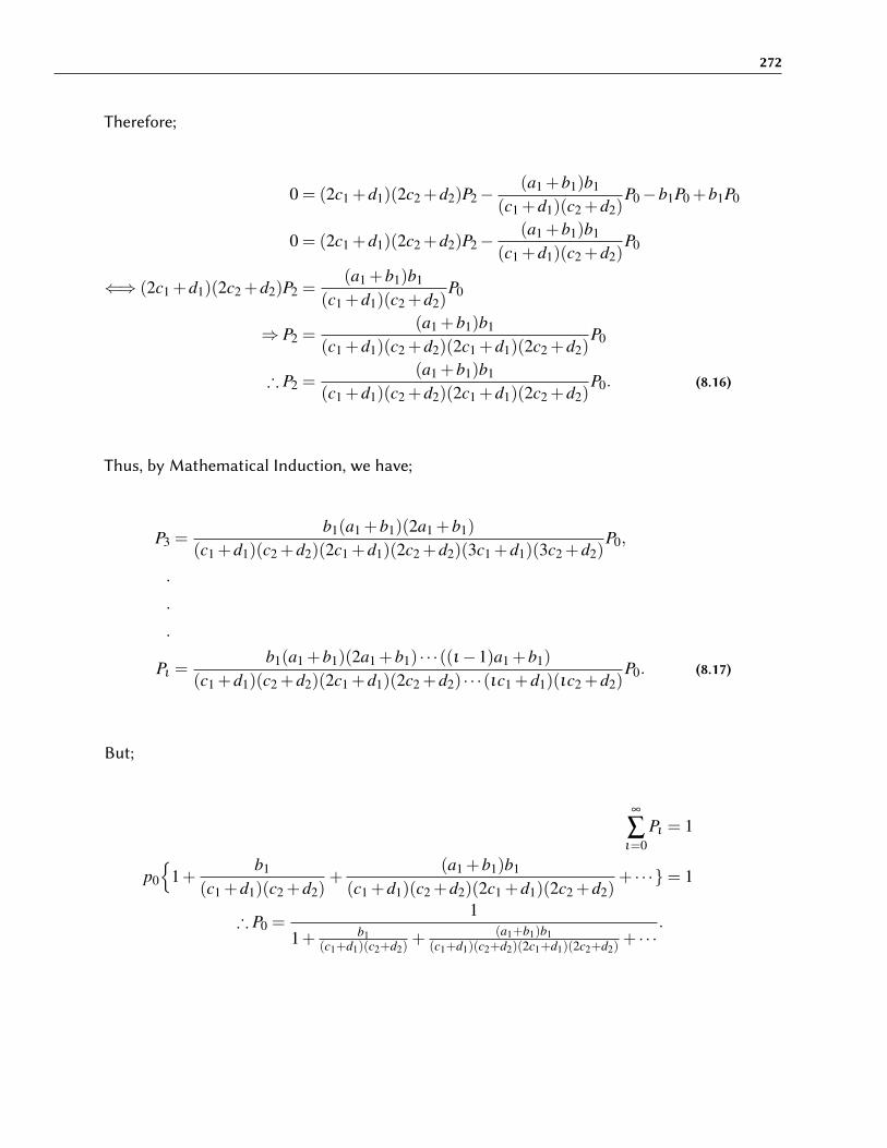
272

Therefore;

0 = (2c1 +d1)(2c2 +d2)P2−(a1 +b1)b1

(c1 +d1)(c2 +d2)P0−b1P0 +b1P0

0 = (2c1 +d1)(2c2 +d2)P2−(a1 +b1)b1

(c1 +d1)(c2 +d2)P0

⇐⇒ (2c1 +d1)(2c2 +d2)P2 =(a1 +b1)b1

(c1 +d1)(c2 +d2)P0

⇒ P2 =(a1 +b1)b1

(c1 +d1)(c2 +d2)(2c1 +d1)(2c2 +d2)P0

∴ P2 =(a1 +b1)b1

(c1 +d1)(c2 +d2)(2c1 +d1)(2c2 +d2)P0. (8.16)

Thus, by Mathematical Induction, we have;

P3 =b1(a1 +b1)(2a1 +b1)

(c1 +d1)(c2 +d2)(2c1 +d1)(2c2 +d2)(3c1 +d1)(3c2 +d2)P0,

.

.

.

Pι =b1(a1 +b1)(2a1 +b1) · · ·((ι−1)a1 +b1)

(c1 +d1)(c2 +d2)(2c1 +d1)(2c2 +d2) · · ·(ιc1 +d1)(ιc2 +d2)P0. (8.17)

But;

∞

∑ι=0

Pι = 1

p0

{1+

b1

(c1 +d1)(c2 +d2)+

(a1 +b1)b1

(c1 +d1)(c2 +d2)(2c1 +d1)(2c2 +d2)+ · · ·}= 1

∴ P0 =1

1+ b1(c1+d1)(c2+d2)

+ (a1+b1)b1(c1+d1)(c2+d2)(2c1+d1)(2c2+d2)

+ · · ·.

273

which is the probability of ultimate extinction.

∴ Pι =b1(a1 +b1)(2a1 +b1) · · ·((ι−1)a1 +b1)

(c1 +d1)(c2 +d2)(2c1 +d1)(2c2 +d2) · · ·(ιc1 +d1)(ιc2 +d2)

x1

1+ b1(c1+d1)(c2+d2)

+ (a1+b1)b1(c1+d1)(c2+d2)(2c1+d1)(2c2+d2)

+ · · ·.

From (8.17);

Pι−1 =b1(a1 +b1)(2a1 +b1) · · ·((ι−2)a1 +b1)

(c1 +d1)(c2 +d2)(2c1 +d1)(2c2 +d2) · · ·((ι−1)c1 +d1)((ι−1)c2 +d2)P0.

∴Pι

Pι−1=

((ι−1)a1 +b1)

(ιc1 +d1)(ιc2 +d2). as required

Let,

Pι =(α1)ι

(γ1)ι(γ2)ι

P0.

where, (α1)ι = α1(α1 +1)(α1 +2) · · ·(α1 + ι−1), ι ≥ 1; (α1)0 = 1,

=Γ(α1 + ι)

Γα1.

and

(γ1)ι = γ1(γ1 +1)(γ1 +2) · · ·(γ1 + ι−1), ι ≥ 1; (γ1)0 = 1,

=Γ(γ1 + ι)

Γγ1,

(γ2)ι =Γ(γ2 + ι)

Γγ2.

α1 =b1

c1, γ1 =

d1

c1+1, γ2 =

d2

c2+1.

The pgf. in hypergeometric term is given by;

φ(z) = 2F1(1,α1;γ1;γ2;ρz)

2F1(1,α1;γ1;γ2;ρ).

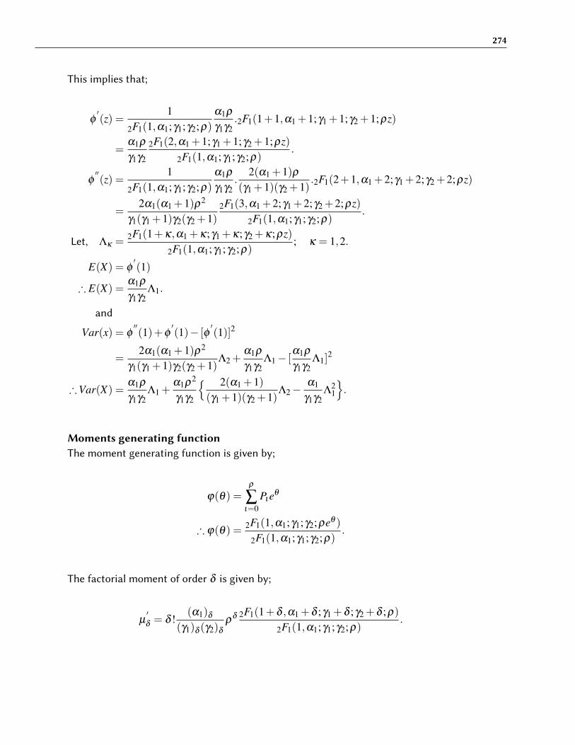
274

This implies that;

φ′(z) =

1

2F1(1,α1;γ1;γ2;ρ)

α1ρ

γ1γ2.2F1(1+1,α1 +1;γ1 +1;γ2 +1;ρz)

=α1ρ

γ1γ2

2F1(2,α1 +1;γ1 +1;γ2 +1;ρz)

2F1(1,α1;γ1;γ2;ρ).

φ′′(z) =

1

2F1(1,α1;γ1;γ2;ρ)

α1ρ

γ1γ2.

2(α1 +1)ρ(γ1 +1)(γ2 +1)

.2F1(2+1,α1 +2;γ1 +2;γ2 +2;ρz)

=2α1(α1 +1)ρ2

γ1(γ1 +1)γ2(γ2 +1)2F1(3,α1 +2;γ1 +2;γ2 +2;ρz)

2F1(1,α1;γ1;γ2;ρ).

Let, Λκ =2F1(1+κ,α1 +κ;γ1 +κ;γ2 +κ;ρz)

2F1(1,α1;γ1;γ2;ρ); κ = 1,2.

E(X) = φ′(1)

∴ E(X) =α1ρ

γ1γ2Λ1.

and

Var(x) = φ′′(1)+φ

′(1)− [φ

′(1)]2

=2α1(α1 +1)ρ2

γ1(γ1 +1)γ2(γ2 +1)Λ2 +

α1ρ

γ1γ2Λ1− [

α1ρ

γ1γ2Λ1]

2

∴Var(X) =α1ρ

γ1γ2Λ1 +

α1ρ2

γ1γ2

{ 2(α1 +1)(γ1 +1)(γ2 +1)

Λ2−α1

γ1γ2Λ

21

}.

Moments generating functionThe moment generating function is given by;

ϕ(θ) =ρ

∑ι=0

Pιeθ

∴ ϕ(θ) =2F1(1,α1;γ1;γ2;ρeθ )

2F1(1,α1;γ1;γ2;ρ).


µ′δ= δ !

(α1)δ

(γ1)δ (γ2)δ

ρδ 2F1(1+δ ,α1 +δ ;γ1 +δ ;γ2 +δ ;ρ)

2F1(1,α1;γ1;γ2;ρ).

275

8.3.3 Case 3: λι = (ιa1 +b1) , µι = (ιc1 +d1)

For λι = (ιa1 +b1) , µι = (ιc1 +d1), the basic di�erence di�erential equations at equilib-rium are:

0 =−b1P0 +(c1 +d1)P1 (8.18)

0 =−{(ιa1 +b1)+ ι(ιc1 +d1)}Pι +(ι +1){(ι +1)c1 +d1}Pι+1 +((ι−1)a1 +b1)Pι−1; ι ≥ 1(8.19)

Hence,

Pι

Pι−1=

(ι)a1 +b1

ι(ιc1 +d1); ι ≥ 1 (8.20)


(c1 +d1)P1 = b1P0

⇒ P1 =b1

(c1 +d1)P0

∴ P1 =b1

(c1 +d1)P0. (8.21)


0 = 2{2c1 +d1}P2−{(a1 +b1)+(c1 +d1)}P1 +b1P0 (8.22)

276


0 =−{(a1 +b1)+(c1 +d1)}.b1

(c1 +d1)P0 +2(2c1 +d1)P2 +b1P0

0 = 2(2c1 +d1)P2−b1(a1 +b1)

(c1 +d1)P0−b1P0 +b1P0

0 = 2(2c1 +d1)P2−b1(a1 +b1)

(c1 +d1)P0

⇐⇒ 2(2c1 +d1)P2 =b1(a1 +b1)

(c1 +d1)P0

⇒ P2 =b1(a1 +b1)

(c1 +d1)2(2c1 +d1)P0

∴ P2 =b1(a1 +b1)

(c1 +d1)2(2c1 +d1)P0.

⇒ P3 =b1(a1 +b1)(2a1 +b1)

(c1 +d1)2(2c1 +d1)3(3c1 +d1)P0,

.

.

.

Pι =b1(a1 +b1)(2a1 +b1) · · ·((ι−1)a1 +b1)

(c1 +d1)2(2c1 +d1) · · · ι(ιc1 +d1)P0; ι ≥ 1 (8.23)

But,

∞

∑ι=0

Pι = 1

⇒ P0 +P1 +P2 · · ·= 1

P0

{1+

b1

(c1 +d1)+

b1(a1 +b1)

(c1 +d1)2(2c1 +d1)· · ·}= 1

∴ P0 =1

1+ b1(c1+d1)

+ b1(a1+b1)(c1+d1)2(2c1+d1)

· · ·


∴ Pι =b1(a1 +b1)(2a1 +b1) · · ·((ι−1)a1 +b1)

(c1 +d1)2(2c1 +d1) · · · ι(ιc1 +d1).

1

1+ b1(c1+d1)

+ b1(a1+b1)(c1+d1)2(2c1+d1)

· · ·.

277


Pι−1 =b1(a1 +b1)(2a1 +b1) · · ·((ι−2)a1 +b1)

(c1 +d1)2(2c1 +d1) · · ·(ι−1)((ι−1)c1 +d1)P0.

∴Pι

Pι−1=

(ι−1)a1 +b1

ι(ιc1 +d1).as required


φ(z) = 1F1(α1;γ1;ρz)

1F1(α1;γ1;ρ).

φ′(z) =

1

1F1(α1;γ1;ρ)

ddz{1F1(α1;γ1;ρz)}

=1

1F1(α1;γ1;ρ)

α1ρ

γ1.1F1(α1;γ1;ρz)

=α1ρ

γ1

1F1(α1 +1;γ1 +1;ρz)

1F1(α1;γ1;ρ).

φ′′(z) =

1

1F1(α1;γ1;ρ)

α1ρ

γ1.

ddz{1F1(α1 +1;γ1 +1;ρz)}

=1

1F1(α1;γ1;ρ)

α1ρ

γ1.(α1 +2)ρ(γ1 +2)

.1F1(α1;γ1;ρz)

=α1(α1 +1)ρ2

γ1(γ1 +1)1F1(α1 +2;γ1 +2;ρz)

1F1(α1;γ1;ρ).

Let, Λκ =1F1(α1 +κ;γ1 +κ;ρz)

1F1(α1;γ1;ρ), κ = 1,2.

E(X) = φ′(1)

∴ E(X) =α1ρ

γ1Λ1.

and

Var(X) = φ′′(1)+φ

′(1)− [φ

′]2

=α1(α1 +1)ρ2

γ1(γ1 +1)Λ2 +

α1ρ

γ1Λ1− [

α1ρ

γ1Λ1]

2

∴Var(X) =α1ρ

γ1Λ1 +

α1ρ2

γ1

(α1 +1γ1 +1

Λ2−α1

γ1Λ

21

).


278

ϕ(θ) =ρ

∑ι=0

Pιeθ

∴ ϕ(θ) =1F1(α1;γ1;ρeθ )

1F1(α1;γ1;ρ).


µ′δ= δ !

(α1)δ

(γ1)δ

ρδ 2F1(α1 +δ ;γ1 +δ ;ρ)

2F1(α1;γ1;ρ).

8.3.4 Case 4: λι = (ιa1 +b1)(ιa2 +b2) , µι = ι(ιc1 +d1)

For λι = (ιa1+b1)(ιa2+b2) , µι = ι(ιc1+d1), the basic di�erence di�erential equationsat equilibrium are:

0 =−(b1b2)P0 +(c1 +d1)P1 (8.24)

0 =−{(ιa1 +b1)(ιa2 +b2)+ ι(ιc1 +d1)}Pι +(ι +1){(ι +1)c1 +d1}Pι+1

+{((ι−1)a1 +b1)((ι−1)a2 +b2)}Pι−1; ι ≥ 1 (8.25)


Pι

Pι−1=

((ι−1)a1 +b1)((ι−1)a2 +b2)

ι(ιc1 +d1); ι ≥ 1 (8.26)


(c1 +d1)P1 = (b1b2)P0

⇒ P1 =b1b1

c1 +d1P0

∴ P1 =b1b1

c1 +d1P0. (8.27)

279


0 = 2(2c1 +d1)P2−{(a1 +b1)(a2 +b2)+(c1 +d1)}P1 +b1b2P0 (8.28)


0 = 2(2c1 +d1)P2−{(a1 +b1)(a2 +b2)+(c1 +d1)}.b1b1

c1 +d1P0 +b1b2P0

0 = 2(2c1 +d1)P2−b1b2(a1 +b1)(a2 +b2)

(c1 +d1)P0−

b1b2

(c1 +d1P0 +

b1b2

(c1 +d1P0

0 = 2(2c1 +d1)P2−b1b2(a1 +b1)(a2 +b2)

(c1 +d1)P0

⇐⇒ 2(2c1 +d1)P2 =b1b2(a1 +b1)(a2 +b2)

(c1 +d1)P0

⇒ P2 =b1b2(a1 +b1)(a2 +b2)

(c1 +d1)2(2c1 +d1)P0

∴ P2 =b1b2(a1 +b1)(a2 +b2)

(c1 +d1)2(2c1 +d1)P0.

⇒ P3 =b1b2(a1 +b1)(a2 +b2)(2a1 +b1)(2a2 +b2)

(c1 +d1)2(2c1 +d1)3(3c1 +d1)P0,

.

.

.

Pι =b1b2(a1 +b1)(a2 +b2) · · ·((ι−1)a1 +b1)((ι−1)a2 +b2)

(c1 +d1)2(2c1 +d1) · · · ι(ιc1 +d1)P0.

(8.29)

280

But,

∞

∑ι=0

Pι = 1

⇒ P0

(1+

b1b1

c1 +d1+

b1b2(a1 +b1)(a2 +b2)

(c1 +d1)2(2c1 +d1)· · ·)= 1

∴ P0 =1

1+ b1b1c1+d1

+ b1b2(a1+b1)(a2+b2)(c1+d1)2(2c1+d1)

· · ·.


From (8.29);

⇒ Pι−1 =b1b2(a1 +b1)(a2 +b2) · · ·((ι−2)a1 +b1)((ι−2)a2 +b2)

(c1 +d1)2(2c1 +d1) · · ·(ι−1)((ι−1)c1 +d1)P0.

∴Pι

Pι−1=

((ι−1)a1 +b1)((ι−1)a2 +b2)

ι(ιc1 +d1); ι ≥ 1. as required


φ(z) = 2F1([1;[2;γ1;ρz)

2F1([1;[2;γ1;ρ).

φ′(z) =

1

2F1([1;[2;γ1;ρ)

ddz{2F1([1;[2;γ1;ρz)}

=1

2F1([1;[2;γ1;ρ)

[1[2ρ

γ1.2F1([1 +1;[2 +1;γ1 +1;ρz)

=[1[2ρ

γ1

2F1([1 +1;[2 +1;γ1 +1;ρz)

2F1([1;[2;γ1;ρ).

φ′′(z) =

1

2F1([1;[2;γ1;ρ)

ddz{2F1([1 +1;[2 +1;γ1 +1;ρz)}

=1

2F1([1;[2;γ1;ρ)

[1[2ρ

γ1.([1 +1)([2 +1)ρ

(γ1 +1).2F1([1 +2;[2 +2;γ1 +2;ρz)

=[1([1 +1)[2([2 +1)ρ2

γ1(γ1 +1)2F1([1 +2;[2 +2;γ1 +2;ρz)

2F1([1;[2;γ1;ρ).

Let, Λκ =2F1([1 +κ;[2 +κ;γ1 +κ;ρz)

2F1([1;[2;γ1;ρ); κ = 1,2.

281

Therefore,

E(X) = φ′(1)

∴ E(X) =[1[2ρ

γ1Λ1.

and

Var(X) = φ′′(1)+φ

′(1)− [φ

′(1)]2

=[1([1 +1)[2([2 +1)ρ2

γ1(γ1 +1)Λ2 +

[1[2ρ

γ1Λ1− [

[1[2ρ

γ1Λ1]

2

∴Var(X) =[1[2ρ

γ1Λ1 +

[1[2ρ2

γ1

{([1 +1)([2 +1)γ1 +1

Λ2−[1[2

γ1Λ

21}.


ϕ(θ) =ρ

∑ι=0

Pιeθ

∴ ϕ(θ) =2F1([1;[2;γ1;ρeθ )

2F1([1;[2;γ1;ρ).


µ′δ= δ !

([1)δ ([2)δ

(γ1)δ

ρδ 2F1([1 +δ ;[2 +δ ;γ1 +δ ;ρ)

2F1([1;[2;γ1;ρ).

8.3.5 Case 5: λι = (ιa1 +b1)(ιa2 +b2) , µι = (ιc1 +d1)(ιc2 +d2)

For λι = (ιa1 +b1)(ιa2 +b2) , µι = (ιc1 +d1)(ιc2 +d2), the basic di�erence di�erentialequations at equilibrium are:

0 =−b1b2P0 +(c1 +d1)(c2 +d2)P1 (8.30)

0 =−{((ι−1)a1 +b1)((ι−1)a2 +b2)}Pι−1−{(ιa1 +b1)(ιa2 +b2)+(ιc1 +d1)(ιc2 +d2)}Pι

+{((ι +1)c1 +d1)((ι +1)c2 +d2)}Pι+1; ι ≥ 1 (8.31)

282


Pι

Pι−1=

((ι−1)a1 +b1)((ι−1)a2 +b2)

(ιc1 +d1)(ιc2 +d2); ι ≥ 1 (8.32)


(c1 +d1)(c2 +d2)P1 = b1b2P0

⇒ P1 =b1b2

(c1 +d1)(c2 +d2)P0

∴ P1 =b1b2

(c1 +d1)(c2 +d2)P0. (8.33)


0 =−b1b2P0−{(a1 +b1)(a2 +b2)+(c1 +d1)(c2 +d2)}P1 +{(2c1 +d1)(2c2 +d2)}P2

(8.34)


0 =−b1b2P0−{(a1 +b1)(a2 +b2)+(c1 +d1)(c2 +d2)}b1b2

(c1 +d1)(c2 +d2)P0

+{(2c1 +d1)(2c2 +d2)}P2

0 = (2c1 +d1)(2c2 +d2)P2−b1b2(a1 +b1)(a2 +b2)

(c1 +d1)(c2 +d2)P0−b1b2P0 +b1b2P0

0 = (2c1 +d1)(2c2 +d2)P2−b1b2(a1 +b1)(a2 +b2)

(c1 +d1)(c2 +d2)P0

283

Therefore,

⇐⇒ (2c1 +d1)(2c2 +d2)P2 =b1b2(a1 +b1)(a2 +b2)

(c1 +d1)(c2 +d2)P0

⇒ P2 =b1b2(a1 +b1)(a2 +b2)

(c1 +d1)(c2 +d2)(2c1 +d1)(2c2 +d2)P0

∴ P2 =b1b2(a1 +b1)(a2 +b2)

(c1 +d1)(c2 +d2)(2c1 +d1)(2c2 +d2)P0.

⇒ P3 =b1b2(a1 +b1)(a2 +b2)(2a1 +b1)(2a2 +b2)

(c1 +d1)(c2 +d2)(2c1 +d1)(2c2 +d2)(3c1 +d1)(3c2 +d2)P0,

.

.

.

Pι =b1b2(a1 +b1)(a2 +b2) · · ·((ι−1)a1 +b1)((ι−1)a2 +b2)

(c1 +d1)(c2 +d2) · · ·(ιc1 +d1)(ιc2 +d2)P0. ι ≥ 1

(8.35)

But,

∞

∑ι=0

Pι = 1

⇒ P0

(1+

b1b2

(c1 +d1)(c2 +d2)+

b1b2(a1 +b1)(a2 +b2)

(c1 +d1)(c2 +d2)(2c1 +d1)(2c2 +d2)+ · · ·

)= 1

∴ P0 =1

1+ b1b2(c1+d1)(c2+d2)

+ b1b2(a1+b1)(a2+b2)(c1+d1)(c2+d2)(2c1+d1)(2c2+d2)

+ · · ·.


Therefore,

Pι =b1b2(a1 +b1)(a2 +b2) · · ·((ι−1)a1 +b1)((ι−1)a2 +b2)

(c1 +d1)(c2 +d2) · · ·(ιc1 +d1)(ιc2 +d2)

x1

1+ b1b2(c1+d1)(c2+d2)

+ b1b2(a1+b1)(a2+b2)(c1+d1)(c2+d2)(2c1+d1)(2c2+d2)

+ · · ·.

284


Pι−1 =b1b2(a1 +b1)(a2 +b2) · · ·((ι−2)a1 +b1)((ι−2)a2 +b2)

(c1 +d1)(c2 +d2) · · ·((ι−1)c1 +d1)((ι−1)c2 +d2)P0.

∴Pι

Pι−1=

((ι−1)a1 +b1)((ι−1)a2 +b2)

(ιc1 +d1)(ιc2 +d2); ι ≥ 1. as required

Its pgf. is given as;

φ(z) = 2F1(1, [1;[2;γ1;γ2;ρz)

2F1(1, [1;[2;γ1;γ2;ρ).

φ′(z) =

1

2F1(1, [1;[2;γ1;γ2;ρ)

ddz{2F1(1, [1;[2;γ1;γ2;ρz)}

=1

2F1(1, [1;[2;γ1;γ2;ρ)

[1[2ρ

γ1γ2.2F1(1+1, [1 +1;[2 +1;γ1 +1;ρz)

=[1[2ρ

γ1γ2

2F1(2, [1 +1;[2 +1;γ1 +1;γ2 +1;ρz)

2F1(1, [1;[2;γ1;γ2;ρ).

φ′′(z) =

1

2F1(1, [1;[2;γ1;γ2;ρ)

ddz{2F1(2, [1 +1;[2 +1;γ1 +1;γ2 +1;ρz)}

=1

2F1(1, [1;[2;γ1;ρ)

[1[2ρ

γ1γ2.2([1 +1)([2 +1)ρ(γ1 +1)(γ2 +1)

.2F1(3, [1 +2;[2 +2;γ1 +2;γ2 +2;ρz)

=2[1([1 +1)[2([2 +1)ρ2

γ1(γ1 +1)γ2(γ2 +1)2F1(3, [1 +2;[2 +2;γ1 +2;γ2 +2;ρz)

2F1(1, [1;[2;γ1;γ2;ρ).

Let, Λκ =2F1(1+κ, [1 +κ;[2 +κ;γ1 +κ;γ2 +κ;ρz)

2F1([1;[2;γ1;ρ); κ = 1,2.

Therefore,

E(X) = φ′(1)

∴ E(X) =[1[2ρ

γ1γ2Λ1.

and

Var(X) = φ′′(1)+φ

′(1)− [φ

′(1)]2

=2[1([1 +1)[2([2 +1)ρ2

γ1(γ1 +1)γ2(γ2 +1)Λ2 +

[1[2ρ

γ1γ2Λ1− [

[1[2ρ

γ1γ2Λ1]

2

∴Var(X) =[1[2ρ

γ1γ2Λ1 +

[1[2ρ2

γ1γ2

{ ([1 +1)([2 +1)(γ1 +1)(γ2 +1)

Λ2−[1[2

γ1γ2Λ

21}.

285


ϕ(θ) =ρ

∑ι=0

Pιeθ

∴ ϕ(θ) =2F1(1, [1;[2;γ1;γ2;ρeθ )

2F1(1, [1;[2;γ1;γ2;ρ).


µ′δ= δ !

([1)δ ([2)δ

(γ1)δ (γ2)δ

ρδ 2F1(1, [1 +δ ;[2 +δ ;γ1 +δ ;γ2 +δ ;ρ)

2F1(1, [1;[2;γ1;γ2;ρ).

8.3.6 Case 6: λι = (ιa1 +b1)(ιa2 +b2) , µι = ι(ιc1 +d1)(ιc2 +d2)

For λι = (ιa1 +b1)(ιa2 +b2) , µι = ι(ιc1 +d1)(ιc2 +d2), the basic di�erence di�erentialequations are:

0 = (c1 +d1)(c2 +d2)P1−b1b2P0 (8.36)

0 = (ι +1){((ι +1)c1 +d1)((ι +1)c2 +d2)}Pι+1−{(ιa1 +b1)(ιa2 +b2)+ ι(ιc1 +d1)(ιc2 +d2)}Pι

+{((ι−1)a1 +b1)((ι−1)a2 +b2)(ι−1)[((ι−1)c1 +d1)((ι−1)c2 +d2)]}Pι−1; ι ≥ 1(8.37)


Pι

Pι−1=

((ι−1)a1 +b1)((ι−1)a2 +b2)

ι(ιc1 +d1)ι(ιc2 +d2); ι ≥ 1 (8.38)


286

(c1 +d1)(c2 +d2)P1 = b1b2P0

⇒ P1 =b1b2

(c2 +d2)(c1 +d1)P0

∴ P1 =b1b2

(c1 +d1)(c2 +d2)P0. (8.39)


0 = 2{(2c1 +d1)(2c2 +d2)}P2−{(c1 +d1)(c2 +d2)+(a1 +b1)(a2 +b2)}P1 +b1b2P0

(8.40)


0 = 2{(2c1 +d1)(2c2 +d2)}P2

−{(c1 +d1)(c2 +d2)+(a1 +b1)(a2 +b2)}.b1b2

(c2 +d2)(c1 +d1)P0

+b1b2P0

0 = 2{(2c1 +d1)(2c2 +d2)}P2−(a2 +b2)b2b1(a1 +b1)

(c2 +d2)(c1 +d1)P0

−b1b2P0 +b1b2P0

⇐⇒ 2{(2c1 +d1)(2c2 +d2)}P2 =(a2 +b2)b2b1(a1 +b1)

(c2 +d2)(c1 +d1)P0

⇒ P2 =(a2 +b2)b2b1(a1 +b1)

(c2 +d2)(c1 +d1)2(2c1 +d1)2(2c2 +d2)P0

∴ P2 =(a2 +b2)b2b1(a1 +b1)

(c2 +d2)(c1 +d1)2(2c1 +d1)2(2c2 +d2)P0.

.

.

.

Pι =b1b2(a1 +b1)(a2 +b2) · · ·((ι−1)a1 +b1)((ι−1)a2 +b2)

(c1 +d1)2(2c2 +d2) · · · ι(ιc1 +d1)ι(ιc2 +d2)P0.

∴Pι

Pι−1=

((ι−1)a1 +b1)((ι−1)a2 +b2)

ι(ιc1 +d1)ι(ιc2 +d2); ι ≥ 1. as require

287


φ(z) = 2F2([1;[2;ζ1;ζ2;ρz)

2F2([1;[2;ζ1;ζ2;ρ).

φ′(z) =

1

2F2([1;[2;ζ1;ζ2;ρ)

ddz{2F2([1;[2;ζ1;ζ2;ρz)}

=1

2F2([1;[2;ζ1;ζ2;ρ)

[1[2ρ

ζ1ζ2.2F2([1 +1;[2 +1;ζ1 +1;ζ2 +1;ρz)

=[1[2ρ

ζ1ζ2

2F2([1 +1;[2 +1;ζ1 +1;ζ2 +1;ρz)

2F2([1;[2;ζ1;ζ2;ρ).

φ′′(z) =

1

2F2([1;[2;ζ1;ζ2;ρ)

[1([1 +1)[2([2 +1)ρ2

ζ1(ζ1 +1)ζ2(ζ2 +1).2F2([1 +2;[2 +2;ζ1 +2;ζ2 +2;ρz)

=[1([1 +1)[2([2 +1)ρ2

ζ1(ζ1 +1)ζ2(ζ2 +1)2F2([1 +2;[2 +2;ζ1 +2;ζ2 +2;ρz)

2F2([1;[2;ζ1;ζ2;ρ).

Let, Λκ =2F2([1 +κ;[2 +κ;ζ1 +κ;ζ2 +κ;ρ)

2F2([1;[2;ζ1;ζ2;ρ); κ = 1,2.

E(X) = φ′(1)

∴ E(X) =[1[2ρ

ζ1ζ2Λ1.

and

Var(X) = φ′′(1)+φ

′(1)− [φ

′(1)]2

=[1([1 +1)[2([2 +1)ρ2

ζ1(ζ1 +1)ζ2(ζ2 +1)Λ2 +

[1[2ρ

ζ1ζ2Λ1−

([1[2ρ

ζ1ζ2Λ1

)2

∴Var(X) =[1[2ρ

ζ1ζ2Λ1 +

[1[2ρ2

ζ1ζ2

( ([1 +1)([2 +1)(ζ1 +1)(ζ2 +1)

Λ2−[1[2

ζ1ζ2Λ

21

).


ϕ(θ) =ρ

∑ι=0

Pιeθ

∴ ϕ(θ) =2F1([1;[2;ζ1;ζ2;ρeθ )

2F1([1;[2;ζ1;ζ2;ρ).

288


µ′δ= δ !

([1)δ ([2)δ

(ζ1)δ (ζ2)δ

ρδ 2F1([1 +δ ;[2 +δ ;ζ1 +δ ;ζ2 +δ ;ρ)

2F1([1;[2;ζ1;ζ2;ρ).

8.3.7 Case 7: λι = (ιa1 +b1)(ιa2 +b2)(ιa3 +b3) , µι = ι(ιc1 +d1)(ιc2 +d2)

For λι = (ιa1 +b1)(ιa2 +b2)(ιa3 +b3) , µι = ι(ιc1 +d1)(ιc2 +d2), the basic di�erencedi�erential equations are:

0 = (c1 +d1)(c2 +d2)P1−b1b2b3P0 (8.41)

0 = (ι +1){((ι +1)c1 +d1)((ι +1)c2 +d2)}Pι+1−{(ιa1 +b1)(ιa2 +b2)(ιa3 +b3)+ ι(ιc1 +d1)(ιc2 +d2)}Pι

+{((ι−1)a1 +b1)((ι−1)a2 +b2)((ι−1)a3 +b3)(ι−1)[((ι−1)c1 +d1)((ι−1)c2 +d2)]}Pι−1; ι ≥ 1(8.42)


Pι

Pι−1=

((ι−1)a1 +b1)((ι−1)a2 +b2)((ι−1)a3 +b3)

ι(ιc1 +d1)ι(ιc2 +d2); ι ≥ 1 (8.43)


(c1 +d1)(c2 +d2)P1 = b1b2b3P0

⇒ P1 =b1b2b3

(c2 +d2)(c1 +d1)P0

∴ P1 =b1b2

(c1 +d1)(c2 +d2)P0. (8.44)

Solving (8.42) iteratively, we have;When ι = 1;

289


0 = 2{(2c1 +d1)(2c2 +d2)}P2−{(c1 +d1)(c2 +d2)+(a1 +b1)(a2 +b2)}P1 +b1b2P0

(8.45)


0 = 2{(2c1 +d1)(2c2 +d2)}P2

−{(c1 +d1)(c2 +d2)+(a1 +b1)(a2 +b2)(a3 +b3)}

xb1b2b3

(c2 +d2)(c1 +d1)P0 +b1b2b3P0

0 = 2{(2c1 +d1)(2c2 +d2)}P2−(a3 +b3)(a2 +b2)b3b2b1(a1 +b1)

(c2 +d2)(c1 +d1)P0

−b1b2b3P0 +b1b2b3P0

⇐⇒ 2{(2c1 +d1)(2c2 +d2)}P2 =(a3 +b3)(a2 +b2)b3b2b1(a1 +b1)

(c2 +d2)(c1 +d1)P0

⇒ P2 =(a3 +b3)(a2 +b2)b3b2b1(a1 +b1)

(c2 +d2)(c1 +d1)2(2c1 +d1)2(2c2 +d2)P0

∴ P2 =(a3 +b3)(a2 +b2)b3b2b1(a1 +b1)

(c2 +d2)(c1 +d1)2(2c1 +d1)2(2c2 +d2)P0.

.

.

.

Pι =b1b2b3(a1 +b1)(a2 +b2) · · ·((ι−1)a2 +b2)((ι−1)a3 +b3)

(c1 +d1)2(2c2 +d2) · · · ι(ιc1 +d1)ι(ιc2 +d2)P0.

∴Pι

Pι−1=

((ι−1)a1 +b1)((ι−1)a2 +b2)((ι−1)a3 +b3)

ι(ιc1 +d1)ι(ιc2 +d2); ι ≥ 1. as require

290


φ(z) = 2F2([1;[2;[3;ζ1;ζ2;ρz)

2F2([1;[2;[3;ζ1;ζ2;ρ).

φ′(z) =

1

2F2([1;[2;[3;ζ1;ζ2;ρ)

ddz{2F2([1;[2;[3;ζ1;ζ2;ρz)}

=1

2F2([1;[2;[3;ζ1;ζ2;ρ)

[1[2[3ρ

ζ1ζ2.2F2([1 +1;[2 +1;[3 +1;ζ1 +1;ζ2 +1;ρz)

=[1[2[3ρ

ζ1ζ2

2F2([1 +1;[2 +1;[3 +1;ζ1 +1;ζ2 +1;ρz)

2F2([1;[2;[3;ζ1;ζ2;ρ).

φ′′(z) =

1

2F2([1;[2;[3;ζ1;ζ2;ρ)

[1([1 +1)[2([2 +1)[3([3 +1)ρ2

ζ1(ζ1 +1)ζ2(ζ2 +1)

.2F2([1 +2;[2 +2;[3 +2;[3 +2;ζ1 +2;ζ2 +2;ρz)

=[1([1 +1)[2([2 +1)[3([3 +1)ρ2

ζ1(ζ1 +1)ζ2(ζ2 +1)2F2([1 +2;[2 +2;[3 +2;ζ1 +2;ζ2 +2;ρz)

2F2([1;[2;[3;ζ1;ζ2;ρ).

Let, Λκ =2F2([1 +κ;[2 +κ;[3 +κ;ζ1 +κ;ζ2 +κ;ρ)

2F2([1;[2;[3;ζ1;ζ2;ρ); κ = 1,2.

E(X) = φ′(1)

∴ E(X) =[1[2[3ρ

ζ1ζ2Λ1.

and

Var(X) = φ′′(1)+φ

′(1)− [φ

′(1)]2

=[1([1 +1)[2([2 +1)[3([3 +1)ρ2

ζ1(ζ1 +1)ζ2(ζ2 +1)Λ2 +

[1[2[3ρ

ζ1ζ2Λ1−

([1[2[3ρ

ζ1ζ2Λ1

)2

∴Var(X) =[1[2[3ρ

ζ1ζ2Λ1 +

[1[2[3ρ2

ζ1ζ2

(([1 +1)([2 +1)([3 +1)(ζ1 +1)(ζ2 +1)

Λ2−[1[2[3

ζ1ζ2Λ

21

).


ϕ(θ) =ρ

∑ι=0

Pιeθ

∴ ϕ(θ) =2F1([1;[2;[3;ζ1;ζ2;ρeθ )

2F1([1;[2;[3;ζ1;ζ2;ρ).

291


µ′δ= δ !

([1)δ ([2)δ ([3)δ

(ζ1)δ (ζ2)δ

ρδ 2F1([1 +δ ;[2 +δ ;[3 +δ ;ζ1 +δ ;ζ2 +δ ;ρ)

2F1([1;[2;[3;ζ1;ζ2;ρ).

9 KEMP’S FAMILIES OF RECURSIVE MODEL INBIRTH AND DEATH PROCESSES AT EQUILIBRIUM

9.1 Introduction

The family of distributions by Kemp can be interpreted in terms of birth-and-death pro-cesses. Suppose that Pn+1

Pnis the ratio of polynomials in n with real roots,

Then;

Pn+1

Pn=

(a1 +n)(a2 +n) · · ·(ap +n)λ(b1 +n)(b2 +n) · · ·(bq+1 +n)

.

where, the coe�icients of the highest powers of n in these polynomials can be assumed tobe unity without loss of generality concerning the form of the resultant distribution.

9.2 A Ratio of a General Linear Recursive Model

Kemp’s (1968) family of distributions is the family of generalized hypergeometric proba-bility distributions have many useful properties.The ratio of two polynomials is given by;Proposition 9.1

Pn+1

Pn=

(a1 +n)(a2 +n) · · ·(ap +n)λ(b1 +n)(b2 +n) · · ·(bq+1 +n)

(9.1)

⇒ (b1 +n)(b2 +n) · · ·(bq+1 +n)Pn+1 = (a1 +n)(a2 +n) · · ·(ap +n)λPn

⇒ (bτ +n)Pn+1 = (aι +n)λPn (9.2)

where, ι = 1,2, · · · , p; τ = 1,2, · · · ,q+1


294

bτP1 = λaιP0

⇒ P1 =aι

bτ

λP0

∴ P1 =aι

bτ

λP0. (9.3)


(bτ +1)P2 = (aι +1)λP1 (9.4)


(bτ +1)P2 = (aι +1)λaι

bτ

λP0

⇒ P2 =aι(aι +1)bτ(bτ +1)

λ2P0

∴ P2 =aι(aι +1)bτ(bτ +1)

λ2P0. (9.5)


(bτ +2)P3 = (aι +2)λP2 (9.6)


(bτ +2)P3 = (aι +2)λaι(aι +1)bτ(bτ +1)

λ2P0

⇒ P3 =aι(aι +1)(aι +2)bτ(bτ +1)(bτ +2)

λ3P0

∴ P3 =aι(aι +1)(aι +2)bτ(bτ +1)(bτ +2)

λ3P0.

295

By Mathematical Induction, we have that;

P4 =aι(aι +1)(aι +2)(aι +3)bτ(bτ +1)(bτ +2)(bτ +3)

λ4P0,

P5 =aι(aι +1)(aι +2)(aι +3)(aι +4)bτ(bτ +1)(bτ +2)(bτ +3)(bτ +4)

λ5P0,

.

.

.

Pn =aι(aι +1)(aι +2) · · ·(aι +n−1)bτ(bτ +1)(bτ +2) · · ·(bτ +n−1)

λnP0. (9.7)

But;

P0 +P1 +P2 +P3 + · · ·= 1

P0 +aι

bτ

λP0 +aι(aι +1)bτ(bτ +1)

λ2P0 +

aι(aι +1)(aι +2)bτ(bτ +1)(bτ +2)

λ3P0 + · · ·= 1

P0

(1+

aι

bτ

λ +aι(aι +1)bτ(bτ +1)

λ2 +

aι(aι +1)(aι +2)bτ(bτ +1)(bτ +2)

λ3 + · · ·

)= 1

∴ P0 =1(

1+ aι

bτλ + aι (aι+1)

bτ (bτ+1)λ2 + aι (aι+1)(aι+2)

bτ (bτ+1)(bτ+2)λ3 + · · ·

) .∴ Pn =

aι(aι +1)(aι +2) · · ·(aι +n−1)bτ(bτ +1)(bτ +2) · · ·(bτ +n−1)

λn.

1(1+ aι

bτλ + aι (aι+1)

bτ (bτ+1)λ2 + aι (aι+1)(aι+2)

bτ (bτ+1)(bτ+2)λ3 + · · ·

) .


Pn+1 =aι(aι +1)(aι +2) · · ·(aι +n−1)(aι +n)bτ(bτ +1)(bτ +2) · · ·(bτ +n−1)(bτ +n)

λn+1P0.

∴Pn+1

Pn=

(aι +n)λ(bτ +n)

, as required. (9.8)

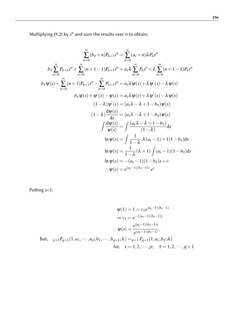
296


∞

∑n=0

(bτ +n)Pn+1sn =∞

∑n=0

(aι +n)λPnsn

bτ

∞

∑n=0

Pn+1sn +∞

∑n=0

(n+1−1)Pn+1sn = aιλ

∞

∑n=0

Pnsn +λ

∞

∑n=0

(n+1−1)Pnsn

bτψ(s)+∞

∑n=0

(n+1)Pn+1sn−∞

∑n=0

Pn+1sn = aιλψ(s)+λψ′(s)−λψ(s)

bτψ(s)+ψ′(s)−ψ(s) = aιλψ(s)+λψ

′(s)−λψ(s)

(1−λ )ψ′(s) = (aιλ −λ +1−bτ)ψ(s)

(1−λ )dψ(s)

ds= (aιλ −λ +1−bτ)ψ(s)∫ dψ(s)

ψ(s)=∫

(aιλ −λ +1−bτ)

(1−λ )ds

lnψ(s) =∫ 1

1−λ.λ (aι −1)+1(1−bτ)ds

lnψ(s) =1

1−λ(λ +1)

∫(aι −1)(1−bτ)ds

lnψ(s) =−(aι −1)(1−bτ)s+ c

∴ ψ(s) = e(aι−1)(bτ−1)s.ec

Pu�ing s=1;

ψ(1) = 1 = c1e(aι−1)(bτ−1)

⇒ c1 = e−{(aι−1)(bτ−1)}

∴ ψ(s) =e(aι−1)(bτ−1)s

e(aι−1)(bτ−1).

But, p+1Fq+1(1,a1, · · · ,ap;b1, · · · ,bq+1;λ ) =p+1 Fq+1(1,aι ;bτ ;λ )

for, ι = 1,2, · · · , p; τ = 1,2, · · · ,q+1

297

Therefore,

p+1Fq+1(1,aι ;bτ ;λ ) = 1+aι

bτ

λ

1!+

1(1+1)aaι(aι +1)bτ(bτ +1)

λ 2

2!+ · · ·+ (1+n−1)(aι +n−1)

(bτ +n−1)λ n

n!

=∞

∑n=0

aι(aι +1) · · ·(aι +n−1)1(1+1) · · ·(1+n−1)bτ(bτ +1) · · ·(bτ +n−1)

λ n

n!

=∞

∑n=0

(aι +n−1) · · ·(aι +1)aι(1+n−1)1(bτ +n−1) · · ·(bτ +1)bτ

λ n

n!

=∞

∑n=0

Γ(1+n)Γ(aι +n)Γ(bτ +n)

Γ(bτ)

Γ(aι)Γ(1)λ n

n!


1 =∞

∑n=0


Γ(bτ)

Γ(aι)Γ(1).

1

p+1Fq+1(1,aι ;bτ ;λ ).λ n

n!

Thus, Pn=Prob (N=n)

=∞

∑n=0


Γ(bτ)

Γ(aι)Γ(1).

1

p+1Fq+1(1,aι ;bτ ;λ ).λ n

n!

Hence, the pgf. is given by;

φ(z) =∞

∑n=0

Pnzn

=∞

∑n=0


Γ(bτ)

Γ(aι)Γ(1)(λ z)n

n!.

1

p+1Fq+1(1,aι ;bτ ;λ )

∴ φ(z) = p+1Fq+1(1,aι ;bτ ;λ z)

p+1Fq+1(1,aι ;bτ ;λ ), ι = 1,2, · · · , p; τ = 1,2, · · · ,q+1; λ > 0. (9.9)

298

Thus;

φ′(z) =

1

p+1Fq+1(1,aι ;bτ ;λ )

ddz.p+1Fq+1(1,aι ;bτ ;λ z)

=1

p+1Fq+1(1,aι ;bτ ;λ )

aι

bτ

λ .p+1Fq+1(1+1,aι +1;bτ +1;λ z)

∴ φ′(z) =

λaι

bτ

p+1Fq+1(2,aι +1;bτ +1;λ z)

p+1Fq+1(1,aι ;bτ ;λ ).

φ′′(z) =

1

p+1Fq+1(1,aι ;bτ ;λ )

2aι(aι +1)bτ(bτ +1)

λ2.p+1Fq+1(2+1,aι +2;bτ +2;λ z)

∴ φ′′(z) =


λ2 p+1Fq+1(3,aι +2;bτ +2;λ z)

p+1Fq+1(1,aι ;bτ ;λ ).

Let, Λκ =p+1Fq+1(1+κ,aι +κ;bτ +κ;λ )

p+1Fq+1(1,aι ;bτ ;λ ), κ = 1,2.

E(X) = φ′(1)

∴ E(X) =λaι

bτ

Λ1.

Var(X) = φ′′(1)+φ

′(1)− [φ

′(1)]2

=2λ 2aι(aι +1)

bτ(bτ +1)Λ2 +

λaι

bτ

Λ1− [λaι

bτ

Λ1]2

∴Var(X) =λaι

bτ

Λ1 +λ 2aι

bτ

[2(aι +1)(bτ +1)

Λ2−aι

bτ

Λ21

].

9.3 Special Cases and Properties

9.3.1 When bq+1 = 1

Suppose that in equation (9.2), one of the denominator parameter is equal to unity, say,bq+1 = 1;Then, we have;Proposition 9.2

Pn+1

Pn=

(a1 +n) · · ·(ap +n)λ(b1 +n) · · ·(bq +n)(n+1)

⇒ (b1 +n) · · ·(bq +n)(n+1)Pn+1 = (a1 +n) · · ·(ap +n)λPn

⇒ (bτ +n)(n+1)Pn+1 = (aι +n)λPn (9.10)

299


bτP1 = aιλP0

⇒ P1 =aι

bτ

λP0

∴ P1 =aι

bτ

λP0. (9.11)


(bτ +1)2P2 = (aι +1)λP1 (9.12)


(bτ +1)2P2 = (aι +1)λaι

bτ

λP0

⇒ P2 =aι(aι +1)bτ(bτ +1)

λ 2

1.2P0

∴ P2 =aι(aι +1)bτ(bτ +1)

λ 2

2!P0. (9.13)


(bτ +2)3P3 = (aι +2)λP2 (9.14)

300


(bτ +2)3P3 = (aι +2)λaι(aι +1)bτ(bτ +1)

λ 2

2!P0

⇒ P3 =aι(aι +1)(aι +2)bτ(bτ +1)(bτ +2)

λ 3

1.2.3P0

∴ P3 =aι(aι +1)(aι +2)bτ(bτ +1)(bτ +2)

λ 3

3!P0.


P4 =aι(aι +1)(aι +2)(aι +3)bτ(bτ +1)(bτ +2)(bτ +3)

λ 4

4!P0,

P5 =aι(aι +1)(aι +2)(aι +3)(aι +4)bτ(bτ +1)(bτ +2)(bτ +3)(bτ +4)

λ 5

5!P0,

.

.

.

Pn =aι(aι +1)(aι +2) · · ·(aι +n−2)(aι +n−1)bτ(bτ +1)(bτ +2) · · ·(bτ +n−2)(bτ +n−1)

λ n

n!P0. (9.15)


Pn+1 =aι(aι +1)(aι +2) · · ·(aι +n−1)(aι +n)bτ(bτ +1)(bτ +2) · · ·(bτ +n−1)(bτ +n)

λ n+1

(n+1)!P0.

Pn+1

Pn=

aι(aι +1)(aι +2) · · ·(aι +n−1)(aι +n)bτ(bτ +1)(bτ +2) · · ·(bτ +n−1)(bτ +n)

λ n.λ 1

(n+1).n!

xbτ(bτ +1)(bτ +2) · · ·(bτ +n−2)(bτ +n−1)aι(aι +1)(aι +2) · · ·(aι +n−2)(aι +n−1)

n!λ n

∴Pn+1

Pn=

(aι +n)λ(bτ +n)(n+1)

, as required.

301

The probability generating function in hypergeometric terms is given by;

φ(z) = pFq(1,aι ;bτ ;λ z)

pFq(1,aι ;bτ ;λ ), ι = 1,2, · · · , p; τ = 1,2, · · · ,q; λ > 0.

φ′(z) =

1

pFq(1,aι ;bτ ;λ )

ddz.pFq(1,aι ;bτ ;λ z)

=1


aι

bτ

λ .pFq(1+1,aι +1;bτ +1;λ z)

∴ φ′(z) =

λaι

bτ

pFq(2,aι +1;bτ +1;λ z)

pFq(1,aι ;bτ ;λ ).

φ′′(z) =

1



λ2.pFq(2+1,aι +2;bτ +2;λ z)

∴ φ′′(z) =


λ2 pFq(3,aι +2;bτ +2;λ z)

pFq(1,aι ;bτ ;λ ).

Let, Λκ =pFq(1+κ,aι +κ;bτ +κ;λ )

pFq(1,aι ;bτ ;λ ), κ = 1,2.

E(X) = φ′(1)

∴ E(X) =λaι

bτ

Λ1.

Var(X) = φ′′(1)+φ

′(1)−{φ

′(1)}2

=2λ 2aι(aι +1)

bτ(bτ +1)Λ2 +

λaι

bτ

Λ1−{λaι

bτ

Λ1}2

∴Var(X) =λaι

bτ

Λ1 +λ 2aι

bτ

{2(aι +1)(bτ +1)

Λ2−aι

bτ

Λ21

}.

10 CONFLUENT HYPERGEOMETRICDISTRIBUTIONS AND THEIR GENERALIZATIONS

10.1 Introduction

In this chapter, a confluent hypergeometric series distribution has been constructed usingKummer‘s series.Its generalization is based on a compound distribution; i.e.,a distribution of a random sumof independent and identically distributed random variables.An integral representation of Kummer‘s series has been used to construct a confluenthypergeometric continuous distribution.Its generalization is based on a confluent hypergeometric series with two variables.Someproperties and special cases of theses distributions have also been discussed.The results in this chapter will help us in solving di�erence-di�erential equations of birthand death processes at equilibrium.

10.2 Bha�acharya’s Confluent Hypergeometric Series Distribution

10.2.1 Construction and Properties

Kummer‘s confluent hypergeometric series is given by:

1F1(ν ;λ ;η) = 1+ν

λ

η

1!+

ν(ν +1)λ (λ +1)

η2

2!+

ν(ν +1)(ν +2)λ (λ +1)(λ +2)

η3

3!+ · · ·

=∞

∑x=0

ν(ν +1)(ν +2) · · ·(ν + x−1)λ (λ +1)(λ +2) · · ·(λ + x−1)

ηx

x!

=∞

∑x=0

(ν + x−1)(ν + x−2) · · ·(ν +2)(ν +1)ν(λ + x−1)(λ + x−2) · · ·(λ +2)(λ +1)λ

Γ(ν)

(λ )

Γ(λ )

Γ(ν)

ηx

x!

=∞

∑x=0

Γ(ν + x)(λ + x)

Γ(λ )

Γ(ν)

ηx

x!(10.1)

For normalizing,we have;

1 =∞

∑x=0

Γ(ν + x)(λ + x)

Γ(λ )

Γ(ν)

1

1F1(ν ;λ ;η)

ηx

x!

304

Therefore,

f (x) = Prob(X = x)

=∞

∑x=0

Γ(ν + x)(λ + x)

Γ(λ )

Γ(ν)

1

1F1(ν ;λ ;η)

ηx

x!for x = 0,1,2, · · · ; ν > 0, λ > 0, η > 0

(10.2)

This result is due to Bha�acharya (1966).The probability generating function (pgf) is givenby:

F(s) =∞

∑x=0

f (x)sx

=∞

∑x=0

Γ(ν + x)(λ + x)

Γ(λ )

Γ(ν)

(ηs)x

x!1

1F1(ν ;λ ;η)

=1F1(ν ;λ ;ηs)

1F1(ν ;λ ;η)(10.3)

∴ F ′(s) =1

1F1(ν ;λ ;η)

dds

(1F1(ν ;λ ;ηs))

=1

1F1(ν ;λ ;η)

ν

λη ∗1 F1(ν +1;λ +1;ηs)

and

F ′′(s) =1

1F1(ν ;λ ;η)

ν

λη ∗ ν +1

λ +1∗η ∗1 F1(ν +2;λ +2;ηs)

=η2

1F1(ν ;λ ;η)

ν(ν +1)λ (λ )+1

∗1 F1(ν +2;λ +2;ηs)

Let

Λ j =1F1(ν + j;λ + j;η)

1F1(ν ;λ ;η); for j = 1,2. (10.4)

∴ E(X) = F ′(1) =ην

λ

1F1(ν +1;λ +1;η)

1F1(ν ;λ ;η)

=ην

λΛ1 (10.5)

and

Var(X) = F ′′(1)+F ′(1)− [F ′(1)]2

= η2 ν(ν +1)

λ (λ +1)Λ2 +

ην

λΛ1−

(ην

λΛ1

)2

=ην

λΛ1 +

η2ν

λ

[ν +1λ +1

Λ2−ν

λΛ

21

](10.6)

305

10.2.2 Special Cases

(i) Poisson Distribution

eθ =∞

∑x=0

θ x

x!=

∞

∑x=0

a(a+1)(a+2) · · ·(a+ x−1)a(a+1)(a+2) · · ·(a+ x−1)

θ x

x!

∴=1 F1(a;a;θ)

∴= e−θ θ x

x!=

1eθ

θ x

x!, x = 0,1,2, · · · ;θ > 0

∴ f (x) =1

1F1(a;a;θ)

θ x

x!

=Γ(a+ x)Γ(a+ x)

Γ(a)Γ(a)

1

1F1(a;a;θ)

θ x

x!for x = 0,1,2, · · · ;θ > 0 (10.7)

Thus, ν = λ = a and η = θ in (10.2)The pgf is;

F(s) = 1F1(a;a;θs)

1F1(a;a;θ)( 10.8)

E(X) = θΛ1 = θ1F1(a;a;θs)

1F1(a;a;θ)= θ (10.9)

and

Var(X) = θΛ1 +θ2(Λ2−Λ

21)

= θ +θ2Λ2−θ

2

= θ +θ2−θ

2

= θ (10.10)

(ii) Displaced Poisson DistributionFrom the expansion of eθ , let us have a partial sum;

S =θ r+1

(r+1)!+

θ r+2

(r+2)!+

θ r+3

(r+3)!+ · · ·

=∞

∑x=0

θ x+r+1

(x+ r+1)!

∴ 1 =∞

∑x=0

θ x+r+1

(x+ r+1)! S

∴ f (x) =θ x+r+1

(x+ r+1)!∑∞x=0

θ x+r+1

(x+r+1)!

for x = 0,1,2, · · · ;θ > 0 (10.11)

306

and r= positive integer.Which is called Displaced Poisson distribution introduced by Sta� (1964).

f (x) =θ x+r+1

(x+ r+1)!∑∞x=0

θ x+r+1

(x+r+1)!

=θ x+r+1

Γ(x+ r)1

∑∞x=0

θ x+r+1

Γ(x+r)

=θ x

Γ(x+ r)1

∑∞x=0

θ x

Γ(x+r)

=θ x

Γ(x+ r)1

∑∞x=0

θ x

x!x!

Γ(x+r)

=θ x

Γ(x+ r)1

∑∞x=0

Γ(1+x)Γ(x+r)

θ x

x!

=θ x

Γ(x+ r)1

∑∞x=0

Γ(1+x)Γ(x+r)

θ x

x!

=θ x

Γ(x+ r)Γ(r)Γ(r)

1

∑∞x=0

Γ(1+x)Γ(x+r)

Γ(r)Γ(r)

θ x

x!

=θ xΓ(r)Γ(x+ r)

1

1F1(1;r;θ)

= x!Γ(r)

Γ(x+ r)1

1F1(1;r;θ)

θ x

x!

=Γ(1+ x)Γ(r+ x)

Γ(r)Γ(1)

1

1F1(1;r;θ)

θ x

x!for x = 0,1,2, · · · ;θ > 0 (10.12)

and r=postive integer.This is f (x) given in (10.2) where v = 1,λ = 1, a positive integer and η = θ > 0

F(s) = 1F1(1;r;θs)

1F1(1;r;θ)( 10.13)

E(X) =θ

rΛ1 (10.14)

and

Var(X) =θ

rΛ1 +

θ 2

r[

2r+1

Λ2−1r

Λ21] (10.15)

where

Λ j =1F1(1+ j;r+ j;θ)

1F1(1;r;θ)for j = 1,2 (10.16)

(iii) Hyper-Poisson DistributionIn the displaced Poisson distribution,we have λ = r is a positive integer.

307

For any λ > 0, we have a hyper Poisson distribution.Bardwell and Crow (1964) termed the distribution Sub-Poisson for λ < 1, Super-Poissonfor λ > 1.Thus,the hyper-Poisson distribution is given by;

f (x) =Γ(1+ x)Γ(λ + x)

Γ(λ )

Γ(1)1

1F1(1;λ ;θ)

θ x

x!for x = 0,1,2, · · · ;λ > 0, θ > 0 (10.17)

∴ F(s) = 1F1(1;λ ;θs)

1F1(1;λ ;θ)( 10.18)

E(X) =θ

λΛ1 (10.19)

and

Var(X) =θ

λΛ1 +

θ 2

λ[

2λ +1

Λ2−1λ

Λ21] (10.20)

where

Λ j =1F1(1+ j;λ + j;θ)

1F1(1;λ ;θ)for j = 1,2 (10.21)

Remark (10.1) Barton (1966) point out that, a hyper-Poisson distribution can be obtainedby considering a truncated Pearson type III mixture of Poisson distribution as shownbelow:We shall first construct the truncated Pearson type III as a mixing distribution.The Pearson di�erential equation is given by;

1y

dydx

=−(a+ x)

c0 + c1x+ c2x2

Where y = f (x), is the pdf of a random variable X and a,c0,c1,c2 are parameters.Pearson type III corresponds to the case of c2 = 0.

308

∴1y

dydx

=−(a+ x)c1x+ c0

=− 1c1

[ x+ax+ c0

c1

]=− 1

c1

[1+

a− c0c1

x+ c0c1

]=− 1

c1−

(a− c0c1)

c1x+ c0

=− 1c1

+

c0c1−a

c1x+ c0

∴ddx

logy =− 1c1

+

c0c1−a

c1x+ c0

∴ logy =∫{− 1

c1+

c0c1−a

c1x+ c0}dx

=− xc1

+− 1c1

+

c0c1−a

c1log(c1x+ c0)+ logk

=− xc1

+ logk(c1x+ c0)α

where

α =

c0c1−a

c1

∴ y = e−x

c1 k(c1x+ c0)α ; c1 6= 0

If c1 > 0, then c1x+ c0 > 0⇒ x >−c0c1

.

If c1 < 0, let c1 =− 1θ

where 1θ> 0

Then,

c1x+ c0 > 0

⇒− xθ+ c0 > 0

⇒− xθ>−c0

⇒ xθ< c0

∴ c1 < 0⇒< θc0

309

Which is the case we wish to consider.

∴ y = eθxk(c0−xθ)α

= eθxk(θc0− x

θ)α

=k

θ αeθx(1− x)α , 0 < x < 1

where θc0 = 1

But y = 1

∴∫ 1

0f (x)dx =

kθ α

∫ 1

0eθx(1− x)αdx

i.e

1 =k

θ α

∫ 1

0eθx(1− x)αdx

∴θ α

k=∫ 1

0x1−1(1− x)α+2−1−1eθxdx

= B(1,α +1)∫ 1

0

x1−1(1− x)α+2−1−1eθx

B(1,α +1)dx

= B(1,α +1) 1F1(1;α +2;θ)

∴k

θ α=

1B(1,α +1) 1F1(1;α +2;θ)

∴ f (x) =eθx(1− x)α

B(1,α +1) 1F1(1;α +2;θ), 0 < x < 1

Let α +2 = β ⇒ α = β −2

∴ f (x) =eθx(1− x)β−2

B(1,β −1) 1F1(1;β ;θ), 0 < x < 1; β > 0

as given by Johnson et al (2005 page 370).As a mixing distribution,we shall use the notations;

g(t) =eθ t(1− t)λ−2

B(1,λ −1) 1F1(1;λ ;θ), for t > 0 (10.23)

which is the truncated Pearson type III.The mixture is given by

310

f (x) =∫ 1

0e−θ t (θ t)x

x!g(t)dt

=∫ 1

0e−θ t (θ t)x

x!eθ t(1− t)λ−2

B(1,λ −1) 1F1(1;λ ;θ)dt

=∫ 1

0

θ x

x!tx(1− t)λ−2

B(1,λ −1) 1F1(1;λ ;θ)dt

=θ x

x!1

B(1,λ −1)1

1F1(1;λ ;θ)

∫ 1

0tx(1− t)λ−1−1dt

=θ x

x!1

B(1,λ −1)1

1F1(1;λ ;θ)B(x+1,λ −1)

=θ x

x!Γ(λ )

Γ(1)Γ(λ −1)1

1F1(1;λ ;θ)

Γ(x+1)Γ(λ −1)λ + x

∴ f (x) =Γ(1+ x)Γ(λ + x)

Γ(λ )

Γ(1)1

1F1(1;λ ;θ)

θ x

x!for x = 0,1,2, · · · ; θ > 0

Which is the hyper-Poisson distribution.Remark (10.2)The truncated Pearson type III distribution can also be derived from a gamma distributiontruncated from above as follows:A two-parameter gamma distribution is given by;

h(y) =θ b

Γbe−θyyb−1, y > 0; θ ,b > 0.

Consider the integral;

I =∫ p

0e−θyyb−1dy

Let θy = x⇒ y =xθ

and dy =dxθ

∴ I =∫

θ p

0e−x(

xθ)b−1 dx

θ

=1

θ b

∫θ p

0e−xxb−1dx

=1

θ b γ(b,θ p)

∴∫

θ p

0e−θyyb−1dy =

γ(b,θ p)θ b

∴∫

θ p

0

γ(b,θ p)θ b e−θyyb−1dy = 1

311

∴ g(y) =∫

θ p

0

γ(b,θ p)θ b e−θyyb−1, 0 < y < p; p > 0; θ > 0; b > 0

But

γ(a,x) =xa

ae−x(1F1(1;a+1;x))

∴ g(y) =θ be−θyyb−1

(θ p)b

b 1F1(1;b+1;θ p)e−θ p

Put p = 1

∴ g(y) =be−θyyb−1

1F1(1;b+1;θ)e−θ

Let,

y = 1− t⇒ dydt

= |−1|= 1

∴ g(t) =be−θ(1−t)(1− t)b−1

1F1(1;b+1;θ)e−θ

=be−θ eθ t(1− t)b−1

1F1(1;b+1;θ)e−θ

=beθ t(1− t)b−1

1F1(1;b+1;θ)

=eθ t(1− t)b−1

B(1,b)1F1(1;b+1;θ)

Let, b+1 = λ ⇒ b = λ −1

∴ g(t) =eθ t(1− t)λ−2

B(1,λ −1)1F1(1;λ ;θ), 0 < t < 1; λ > 0

Which is a truncated Pearson type III distribution.

10.3 Extended Confluent Hypergeometric Series (ECHS) Distribution

10.3.1 Compound Distribution

Let SY = X1 +X2 + · · ·+XY

Where the Xi′s are iid random variables.Further,let Y also be a random variable independent of Xi′s.IfH(s)=the probability generating function of SY = E[SSY ]

F(s)=the probability generating function of Y = E[SY ]

G(s)=the probability generating function of Xi = E[SXi]

Then;

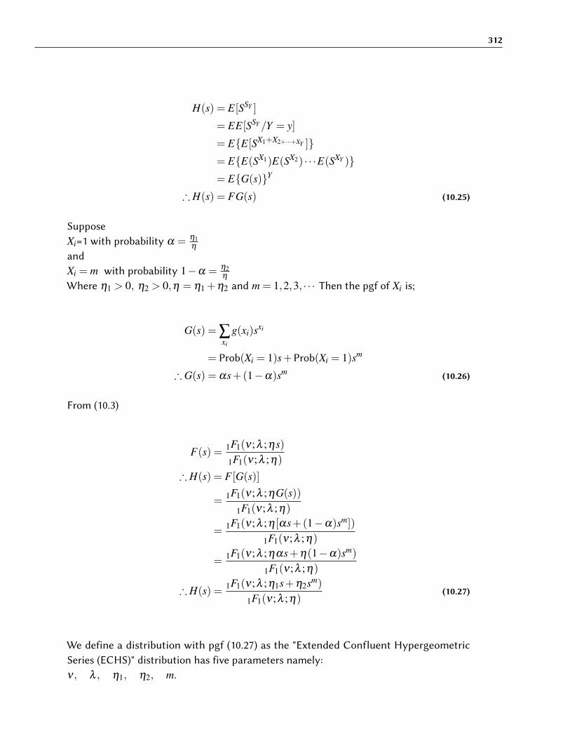
312

H(s) = E[SSY ]

= EE[SSY /Y = y]

= E{E[SX1+X2+···+XY ]}= E{E(SX1)E(SX2) · · ·E(SXY )}= E{G(s)}Y

∴ H(s) = FG(s) (10.25)

SupposeXi=1 with probability α = η1

η

andXi = m with probability 1−α = η2

η

Where η1 > 0, η2 > 0,η = η1 +η2 and m = 1,2,3, · · · Then the pgf of Xi is;

G(s) = ∑xi

g(xi)sxi

= Prob(Xi = 1)s+Prob(Xi = 1)sm

∴ G(s) = αs+(1−α)sm (10.26)

From (10.3)

F(s) = 1F1(ν ;λ ;ηs)

1F1(ν ;λ ;η)

∴ H(s) = F [G(s)]

=1F1(ν ;λ ;ηG(s))

1F1(ν ;λ ;η)

=1F1(ν ;λ ;η [αs+(1−α)sm])

1F1(ν ;λ ;η)

=1F1(ν ;λ ;ηαs+η(1−α)sm)

1F1(ν ;λ ;η)

∴ H(s) = 1F1(ν ;λ ;η1s+η2sm)

1F1(ν ;λ ;η)(10.27)

We define a distribution with pgf (10.27) as the "Extended Confluent HypergeometricSeries (ECHS)" distribution has five parameters namely:ν , λ , η1, η2, m.

313

∴ H ′(s) =1

1F1(ν ;λ ;η)

dds 1F1(ν ;λ ;η1s+η2sm)

=1

1F1(ν ;λ ;η)

ν

λ(η1 +mη2sm−1) 1F1(ν +1;λ +1;η1s+η2sm)

H ′′(s) =1

1F1(ν ;λ ;η)

ν

λ{m(m−1)η2sm−2

1F1(ν +1;λ +1;η1s+η2sm)

+(η1 +mη2sm−1)2 ν +1λ +1 1F1(ν +2;λ +2;η1s+η2sm)}

Let

∴ Λ j =1F1(ν + j;λ + j;η1)

1F1(ν ;λ ;η), for j = 1,2 (10.28)

∴ E[SY ] = H ′(1) =ν

λ(η1 +mη2)

1F1(ν +1;λ +1;η1 +η2)

1F1(ν ;λ ;η)

E[SY ] =ν

λ(η1 +mη2)Λ1 (10.29)

Var[SY ] = H ′′(1)+H ′(1)− [H ′(1)]2

=1

1F1(ν ;λ ;η)

ν

λ

{m(m−1)η2 1F1(ν +1;λ +1;η1 +η2)

+(η1 +mη2)2 ν +1

λ +11F1(ν +2;λ +2;η)

1F1(ν ;λ ;η)

}ν

λ(η1 +mη2)Λ1−

ν2

λ 2 (η1 +mη2)2Λ

21

=ν

λm(m−1)η2Λ2 +(η1 +mη2)

2 ν

λ

ν +1λ +1

Λ1

+ν

λ(η1 +mη2)Λ1−

ν2

λ 2 (η1 +mη2)2Λ

21

∴Var[SY ] =ν

λ[m2

η2−mη2 +η1 +mη1]Λ1 +ν

λ(η1 +mη2)

2[ν +1λ +1

Λ2−ν

λΛ

21]

∴Var[SY ] =ν

λ(η1 +m2

η2)Λ1 +ν

λ(η1 +mη2)

2(ν +1λ +1

Λ2−η

λΛ

21) (10.30)

10.3.2 Recursion in Extended Confluent Hypergeometric Series Distributions

(a) A recursive formula for probabilitiesThe random variable under consideration is SY

Leth j = Prob {SY = j} ≡ h j(ν ,λ )

Hence the pgf is:

314

H(s) =∞

∑j=0

h j(ν ,λ )s j (10.31)

i.e

1F1(ν ;λ ;η1s+η2sm)

1F1(ν ;λ ;η)=

∞

∑j=0

h j(ν ,λ )s j (10.32)

Di�erentiating (10.32) with respect to s, we have;

ν

λ

[1F1(ν +1;λ +1;η1s+η2sm)](η1 +mη2sm−1)

1F1(ν ;λ ;η)=

∞

∑j=0

jh j(ν ,λ )s j−1

=∞

∑j=1

jh j(ν ,λ )s j−1

=∞

∑j=0

( j+1)h j+1(ν ,λ )s j (10.33)

Replacing ν = ν +1, λ = λ +1 in (10.32) we have;

1F1(ν +1;λ +1;η1s+η2sm)

1F1(ν +1;λ +1;η)=

∞

∑j=0

h j(ν +1,λ +1)s j (10.34)

Divide (10.33) by (10.34), we have;

ν

λ(η1 +mη2sm−1)

1F1(ν +1;λ +1;η)

1F1(ν ;λ ;η)=

∑∞j=0( j+1)h j+1(ν ,λ )s j

∑∞j=0 h j(ν +1,λ +1)s j

Let 1F1(ν +1;λ +1;η)

1F1(ν ;λ ;η)= Λ1

∴ν

λ(η1 +mη2sm−1)Λ1 =

∑∞j=0( j+1)h j+1(ν ,λ )s j

∑∞j=0 h j(ν +1,λ +1)s j

∴ν

λΛ1{

∞

∑j=0

η1h j(ν +1,λ +1)s j +∞

∑j=0

mη2h j(ν +1,λ +1)sm+ j−1}=∞

∑j=0

( j+1)h j+1(ν ,λ )s j

(10.35)

Comparing the coe�icient of sr in (6.35) we have:For the Right Hand Side,the coe�icient=(r+1)hr+1(ν ,λ ) by pu�ing j = r

315

For the Le� Hand Side,put j = s for the first term to get;

ν

λΛ1η1hr(ν +1,λ +1).

Put m+ j−1 = r⇒ j = r−m+1 for the second term to get;

mη2ν

λΛ1hr−m+1(ν +1,λ +1)

Thus we have;

(r+1)hr+1(ν ,λ ) =ν

λΛ1{η1hr(ν +1,λ +1)+mη2hr−m+1(ν +1,λ +1)} (10.36)

when r ≥ m

and

(r+1)hr+1(ν ,λ ) =ν

λΛ1η1hr(ν +1,λ +1) (10.37)

when r < m.

(b) A recursive formula for factorial momentsConsider;

H(1+ s) =∞

∑j=0

h j(ν ,λ )(1+ s) j (10.38)

i.e

1F1(ν ;λ ;η1(1+ s)+η2(1+ s)m)

1F1(ν ;λ ;η)=

∞

∑j=0

h j(ν ,λ )(1+ s) j

=∞

∑j=0

{h j(ν ,λ )

j

∑n=0

(jn

)(s)n}

=∞

∑j=0

∞

∑n=0

h j(ν ,λ )

(jn

)(s)n

=∞

∑n=0

{[

∞

∑j=0

j!( j−n)!

h j(ν ,λ )]sn

n!

}=

∞

∑n=0

{[

∞

∑j=0

j( j−1)( j−2) · · ·( j−n+1)h j(ν ,λ )]sn

n!

}=

∞

∑n=0

µn(ν ,λ )sn

n!(10.39)

316

Di�erentiating (10.39) with respect to s, we get;

ν

λ

[1F1(ν +1;λ +1;η1(1+ s)+η2sm)](η1 +mη2(1+ s)m−1)

1F1(ν ;λ ;η)=

∞

∑n=0

µn(ν ,λ )sn−1

(n−1)!

=∞

∑n=0

µn+1(ν ,λ )sn

n!(10.40)

Replacing ν = ν +1, λ = λ +1 in (10.39) we get;

1F1(ν +1;λ +1;η1(1+ s)+η2(1+ s)m)

1F1(ν +1;λ +1;η)=

∞

∑n=0

µn(ν +1,λ +1)sn

n!(10.41)

Divide (10.40) by (10.41) to get;

ν

λΛ1[η1 +mη2(1+ s)m−1] =

∑∞n=0 µn+1(ν ,λ )

sn

n!

∑∞n=0 µn(ν +1,λ +1) sn

n!

∴∞

∑n=0

µn+1(ν ,λ )sn

n!=

ν

λΛ1

∞

∑n=0

η1µn(ν +1,λ +1)sn

n!

+ν

λΛ1

∞

∑n=0

mη2(1+ s)m−1µn(ν +1,λ +1)

sn

n!

=ν

λΛ1

∞

∑n=0


n!

+ν

λΛ1

∞

∑n=0

{mη2

m−1

∑j=0

(m−1

j

)s j

µn(ν +1,λ +1)sn

n!

}=

ν

λΛ1

∞

∑n=0


n!

+ν

λΛ1

∞

∑n=0

{mη2

m−1

∑j=0

(m−1

j

)s j

µn(ν +1,λ +1)s j+n

n!

}(10.42)

Comparing the coe�icient of sn in (10.42) we have;For the LHS put n = r to get,

µ[r+1](ν ,λ )

r!

317

For the RHS,put n = r for the first term to get,

ν

λΛ1η1µ[r](ν +1,λ +1)

r!

Put j+n = r⇒ n = r− j to get;

ν

λΛ1mη2

m−1

∑j=0

(m−1

j

)µ[r− j](ν +1,λ +1)

(r− j)!

∴µ[r+1](ν ,λ )

r!=

ν

λΛ1η1µ[r](ν +1,λ +1)+

ν

λΛ1mη2

m−1

∑j=0

(m−1

j

)µ[r− j](ν +1,λ +1)

(r− j)!

∴ µ[r+1](ν ,λ ) =ν

λΛ1

{η1µ[r](ν +1,λ +1)+mη2

m−1

∑j=0

r j(

m−1j

)µ[r− j](ν +1,λ +1)

}(10.43)

where r j = r(r−1)(r−2) · · ·(r− j+1)

(b) Recursive formula for the rth momentsThe characteristic function of SY is;

QSY (t) = E[eitSY ]

= E[e(it)SY ]

= H[eit ]

∴ QSY (t) =1F1(ν ;λ ;η1eit +η2emit)

1F1(ν ;λ ;η)(10.44)

And since H(s) = ∑ j(ν ,λ )s j

Then,

H(eit) = ∑j(ν ,λ )eit j

=∞

∑j=0{h j(ν ,λ )

∞

∑n=0

(it j)n

n!}

=∞

∑n=0{[

∞

∑j=0

jnh j(ν ,λ )](it)n

n!}

∴ H(eit) =∞

∑n=0

µ′n(ν ,λ )

(it)n

n!(10.45)

318

Therefore,

1F1(ν ;λ ;η1eit +η2emit)

1F1(ν ;λ ;η)=

∞

∑n=0

µ′n(ν ,λ )

(it)n

n!(10.46)

Di�erentiating (10.46) with respect to t,we get;

ν

λ 1F1(ν +1;λ +1;η1eit +η2emit)[iη1eit +miη2emit ]

1F1(ν ;λ ;η)=

∞

∑n=1

µ′n(ν ,λ )

intn−1

(n−1)!(10.47)

Replacing ν = ν +1, λ = λ +1 in (10.46) we get;

1F1(ν +1;λ +1;η1eit +η2emit)

1F1(ν +1;λ +1;η)=

∞

∑n=0

µ′n(ν +1,λ +1)

(it)n

n!(10.48)

Next divide (10.47) by (10.48) to get;

ν

λΛ1[iη1eit +miη2emit ] =

∑∞n=1 µ ′n(ν ,λ )

intn−1

(n−1)!

∑∞n=0 µ ′n(ν +1,λ +1) (it)

n

n!

=∑

∞n=0 µ ′n+1(ν ,λ )

in+1tn

(n)!

∑∞n=0 µ ′n(ν +1,λ +1) (it)

n

n!

∴ν

λΛ1[η1eit +mη2emit ] =

∑∞n=0 µ ′n+1(ν ,λ )

(it)n

(n)!

∑∞n=0 µ ′n(ν +1,λ +1) (it)

n

n!

Therefore,

∞

∑n=0

µ′n+1(ν ,λ )

(it)n

(n)!=

ν

λΛ1{

∞

∑n=0

η1eitµ′n(ν +1,λ +1)

(it)n

n!

+∞

∑n=0

mη2emitµ′n(ν +1,λ +1)

(it)n

n!}

=ν

λΛ1{

∞

∑n=0

[η1µ′n(ν +1,λ +1)

∞

∑k=0

(it)k

k!(it)n

n!]

+∞

∑n=0

[mη2µ′n(ν +1,λ +1)

∞

∑k=0

(mit)k

k!(it)n

n!]}

319

Therefore,

∞

∑n=0

µ′n+1(ν ,λ )

(it)n

(n)!=

ν

λΛ1{

∞

∑n=0

[η1µ′n(ν +1,λ +1)

∞

∑k=0

(it)k+n

k!n!]

+∞

∑n=0

[mη2µ′n(ν +1,λ +1)

∞

∑k=0

mk(it)k+n

k!n!]}

∞

∑n=0

µ′n+1(ν ,λ )

(it)n

(n)!=

ν

λΛ1

∞

∑n=0

∞

∑k=0{(η1 +mη2mk)

µ ′n(ν +1,λ +1)(it)k+n

k!n!} (10.49)

Comparing the coe�icient of (it)r, we have;From LHS by pu�ing n = r

µ ′r+1(ν ,λ )

r!

Pu�ing k+n = r,⇒ n = r− k we have;From RHS:

ν

λΛ1

∞

∑k=0

(η1 +mη2mk)µ ′r−k(ν +1,λ +1)

k!(r− k)!

Therefore,

µ ′r+1(ν ,λ )

r!=

ν

λΛ1

∞

∑k=0

(η1 +mη2mk)µ ′r−k(ν +1,λ +1)

k!(r− k)!

∴ µ′r+1(ν ,λ ) =

ν

λΛ1

∞

∑k=0

(rk

)(η1 +mη2mk)µ ′r−k(ν +1,λ +1)

∴ µ′r+1(ν ,λ ) =

ν

λΛ1

∞

∑k=0

(rk

)(η1 +η2mk+1)µ ′r−k(ν +1,λ +1)

10.3.3 Probability mass function of the Extended Confluent Hypergeometric Se-ries (ECHS) Distributions

320

Again, let

H(s) =∞

∑x=0

hx(ν ,λ )sx

i.e

1F1(ν ;λ ;η1s+η2sm)

1F1(ν ;λ ;η)=

∞

∑x=0

hx(ν ,λ )sx

i.e

1

1F1(ν ;λ ;η)

∞

∑x=0

ν(ν +1)(ν +2) · · ·(ν + x−1)λ (λ +1)(λ +2) · · ·(λ + x−1)

(η1s+η2sm)x

x!=

∞

∑x=0

hx(ν ,λ )sx

∴1

1F1(ν ;λ ;η)

∞

∑x=0

(ν)x

(λ )x

(η1s+η2sm)x

x!=

∞

∑x=0

hx(ν ,λ )sx (10.51)

Where (a)0 = 1 and (a)n = a(a+1)(a+2) · · ·(a+n−1) for n≥ 1We can rewrite (10.51) as;

∞

∑x=0

hx(ν ,λ )sx =1

1F1(ν ;λ ;η)

∞

∑x=0{ (ν)x

(λ )x

∞

∑n=0

(xn

)(η1s)x−n

x!(η2sm)n}

∴∞

∑x=0

hx(ν ,λ )sx =1

1F1(ν ;λ ;η)

∞

∑x=0

∞

∑n=0

(ν)x

(λ )x

ηx−n1 ηn

2 sx−n+mn

(x−n)!n!

Comparing the coe�icient of Sr,

Put x = r on the LHS to get hr(ν ,λ )

Put x−n+mn = r on the RHS .Therefore, x = r− (m−1)n.THerefore,the coe�icient of Sr on the RHS is;

1

1F1(ν ;λ ;η)

∞

∑n=0

(ν)r−(m−1)n

(λ )r−(m−1)n

ηr−mn1 ηn

2(r−mn)!n!

Therefore,

hr(ν ,λ ) =1

1F1(ν ;λ ;η)

∞

∑n=0

(ν)r−(m−1)n

(λ )r−(m−1)n

ηr−mn1 ηn

2(r−mn)!n!

(10.52)

10.4 Special Cases of ECHS (ν ,m,η1,η2) Distribution

For each case,we determine the pgf,mean and the variance using formulae (10.27),(10.29)and (10.30) respectively.

321

10.4.1 When η2 = 0

Then

H(s) = 1F1(ν ;λ ;η1s)

1F1(ν ;λ ;η1)

Which is the pgf of Bha�acharya‘s Confluent Hypergeometric Series distribution givenby (10.3)

E[SY ] =ν

λη1Λ1

and

Var[SY ] =ν

λη1Λ1 +

ν

λη1(

ν +1λ +1

Λ2−ν

λΛ

21)

Where, Λ j =1F1(ν + j;λ + j;η1)

1F1(ν ;λ ;η1)

10.4.2 When ν = λ ,m = 2;η1 > 0,η2 > 0 = 0

THen,

H(s) = 1F1(ν ;λ ;η1s+η2s2)

1F1(ν ;λ ;η)

Which is the pgf of the Hermite distribution due to Kemp and Kemp (1965).

E[SY ] = (η1 +2η2)Λ1

and

Var[SY ] = (η1 +4η2)Λ1 +(η1 +2η2)2(Λ2−Λ

21)

Where, Λ j =1F1(λ + j;λ + j;η)

1F1(λ ;λ ;η)

Remark (10.3)

The pgf of a Hermite distribution is a Compound Poisson distribution obtained by consid-eringSN = X1 +X2 + · · ·+XN

322

Where X si are iid binomial random variables with parameters 2 and p.

N is poisson with parameter λ .

∴ H(s) = eλ [G(s)−1] = eλ [(q+ps)2−1]

∴ H(s) = exp{λ [q2 + p2s2 +2qps−1]}= exp{λ [q2 + p2− p2 + p2s2 +2qps−1]}= exp{λ [(q+ p)2 + p2(s2−1)+2qps−1]}= exp{λ [(q+ p)2−2qp+ p2(s2−1)+2qps−1]}= exp{λ [1−2qp+ p2(s2−1)+2qps−1]}= exp{λ [2qp(s−1)+ p2(s2−1)]}

∴ H(s) = eλ [2qps−2qp+p2s2−p2]

= eλ [(2qps+p2s2)−(2qp+p2)]

= e(2λqps+λ p2s2)e−λ (2qp+p2)

∴ H(s) =e2λqps+λ p2s2

e2λqp+λ p2

From section (10.2.2),we found tha;

eθ =1 F1(a;a;θ)

∴ H(s) = 1F1(a;a;2λqps+λ p2s2)

1F1(a;a;2λqp+λ p2)

=1F1(λ ;λ ;2λqps+λ p2s2)

1F1(λ ;λ ;2λqp+λ p2)

=1F1(λ ;λ ;η1s+η2s2)

1F1(λ ;λ ;η1 +η2)

=1F1(λ ;λ ;η1s+η2s2)

1F1(λ ;λ ;η)

Where, η1 = 2λqp, η2 = λ p2; η = η1 +η2, ν = λ , m = 2

Remark (10.4)

323

A Hermite distribution is a discrete Poisson mixture as shown below:

Let, h j = Prob{SN = j}= ∑

nProb{SN = j,N = n}

= ∑n

Prob{SN = j/N = n}Prob{N = n}

= ∑n

Prob{X1 +X2 + · · ·+Xn = j}Prob{N = n}

= ∑n{ f j}n∗Pn

Where { f j}n∗ is an n-th fold convolution Xi

In terms of pgf;

H(s) =∞

∑j=0

h js j = ∑n[G(s)]nPn

Where G(s) is the pgf of XisIf Xi ∼ Bin(2, p) and N ∼ Poiss(λ )THen,

H(s) =∞

∑n=0

[(q+ ps)2]ne−λλ n

n!

= e−λ∞

∑n=0

[(q+ ps)2]n

n!

= e−λ eλ (q+ps)2

= exp{−λ +λq2 +2λ pqs+λ p2s2}= exp{−λ +λq2 +2λ pqs+λ p2s2−λ p2 +λ p2}= exp{−λ +λq2 +2λ pqs+λ p2(s2−1)}= exp{−λ +2λ pqs+λ (p2 +q2)+λ p2(s2−1)}

∴ H(s) = exp{−λ +2λ pqs+λ (p2 +q2 +2pq−2pq)+λ p2(s2−1)}= exp{−λ +2λ pqs+λ [(p+q)2−2pq]+λ p2(s2−1)}= exp{−λ +2λ pqs+λ −2λ pq+λ p2(s2−1)}

∴ H(s) = exp{2λ pq(s−1)+λ p2(s2−1)}

324

Which is a pgf of a Hermite distribution that can be wri�en as;

H(s) = e2λ pqs−2λ pq+λ p2s2−λ p2

=e2λ pqs+λ p2s2

e2λ pq+λ p2

∴ H(s) = 1F1(λ ;λ ;2λ pqs+λ p2s2)

1F1(λ ;λ ;2λ pq+λ p2)

Remark (10. 5)

Kemp and Kemp (1966) found that if mixing is treated purely as a formal process with thePoisson parameter θ taking negative values,then a Hermite distribution can be derivedas a Poisson-Normal mixture as follows:

325

H(s) =∫

∞

−∞

e−θ(1−s) 1√

2πσ2e− (θ−µ)2

2σ2

dθ

=1√

2πσ2

∫∞

−∞

exp{−θ(1− s)− (θ −µ)2

2σ2 }dθ

=1√

2πσ2

∫∞

−∞

exp{−2θ(1− s)σ2− (θ −µ)2

2σ2 }dθ

=1√

2πσ2

∫∞

−∞

exp{−2θ(1− s)σ2− [θ 2−2µθ +µ2]

2σ2 }dθ

=1√

2πσ2

∫∞

−∞

exp{− 12σ2 [2σ

2(1− s)θ +θ2−2µθ +µ

2]}dθ

=1√

2πσ2

∫∞

−∞

exp{− 12σ2 [θ

2−2{µ−σ2(1− s)}θ +µ

2]}dθ

=1√

2πσ2

∫∞

−∞

exp{− 12σ2 [{θ −µ +σ

2(1− s)}2−{µ−σ2(1− s)}2 +µ

2]}dθ

= exp{− 12σ2 [µ

2−{µ−σ2(1− s)}2]}.1

= exp{− 12σ2 [2µ−σ

2(1− s)][σ2(1− s)]}

= exp{−12[2µ−σ

2(1− s)](1− s)}

= exp{−12[2µ(1− s)−σ

2(1− s)2]}

= exp{−12[2µ(1− s)−σ

2(1−2s+ s2−1+1)]}

= exp{−12[2µ(1− s)−σ

2(2−2s+ s2−1)]}

= exp{−12[2µ(1− s)−2σ

2(1− s)−σ2(s2−1)]}

= exp{−12[2(µ−σ

2)(1− s)−σ2(s2−1)]}

∴ H(s) = exp{(µ−σ2)(s−1)+

σ2

2(s2−1)}

Which is a pgf of a Hermite distribution.

10.4.3 When ν = λ , m > 0; η1 > 0, η2 > 0

Then,

H(s) = 1F1(λ ;λ ;η1s+η2sm)

1F1(λ ;λ ;η)

326

which is the pgf of the generalized Hermite distribution due to Gupta and Jain (1974).

E[SY ] = (η1 +mη2)Λ1

and

Var[SY ] = (η1 +m2η2)Λ1 +(η1 +mη2)(Λ2−Λ

21)

where Λ j =1F1(λ + j;λ + j;η)

1F1(λ ;λ ;η), j = 1,2

Remark(10.6)

In constructing a generalized Hermite distribution,Gupta and Jain (1974) considered thevariable x given by;X = X1 +mX2

Where X1+mX2 are independent Poisson random variable with parameter η1 and η2 respectively.The pgf of X is;

H(s) = E[SX1+mX2]

= E(SX1)E(SmX2)

= e−η1(1−s)e−η2(1−sm)

= e−η1+η1s−η2+η2sm

= eη1s+η1sm−η1−η2

=eη1s+η1sm

eη1+η2

=1F1(λ ;λ ;η1s+η2sm)

1F1(λ ;λ ;η1 +η2)

∴ H(s) = 1F1(λ ;λ ;η1s+η2sm)

1F1(λ ;λ ;η)

10.4.4 When ν = 1, m = 2 and λ = λ

a positive integer,Then

H(s) = 1F1(λ ;λ ;η1s+η2s2)

1F1(λ ;λ ;η)

which is the pgf of the extended displaced Poisson distribution of type I with parame-ters λ , η1 > 0 and η2 > 0

327

E[SY ] =1λ(η1 +2η2)Λ1

and

Var[SY ] =1λ(η1 +4η2)Λ1 +

1λ(η1 +2η2)

2(2

λ +1Λ1−

1λ

Λ21)

where Λ j =1F1(1+ j;λ + j;η)

1F1(1;λ ;η), j = 1,2

10.4.5 When ν = 1, λ = rand m≥ 2

where r is a positive integer,Then

H(s) = 1F1(1;r;η1s+η2sm)

1F1(1;r;η)

which is the pgf of the extended displaced Poisson distribution of type II with parame-ters λ , m, η1 > 0 and η2 > 0

E[SY ] =1r(η1 +mη2)Λ1

and

Var[SY ] =1r(η1 +mη2)Λ1 +

1r(η1 +mη2)

2(2

r+1Λ2−

1r

Λ21)

where Λ j =1F1(1+ j;r+ j;η)

1F1(1;r;η), j = 1,2

10.4.6 When m = 2

Then

H(s) = 1F1(ν ;λ ;η1s+η2s2)

1F1(ν ;λ ;η)

which is the pgf of the extended Bardwell and Crow family of distributions of type IIIwith parameters ν > 0, λ > 0, η1 > 0 and η2 > 0

328

E[SY ] =ν

λ(η1 +2η2)Λ1

and

Var[SY ] =ν

λ(η1 +4η2)Λ1 +

ν

λ(η1 +2η2)

2(ν +1λ +1

Λ2−ν

λΛ

21)

where Λ j =1F1(ν + j;λ + j;η)

1F1(ν ;λ ;η), j = 1,2

10.4.7 When ν = 1

Then

H(s) = 1F1(1;λ ;η1s+η2s2)

1F1(1;λ ;η)

which is the pgf of the extended Crow-Bardwell family of distributions of type II withparameters m > 0, ,λ > 0, η1 > 0 and η2 > 0

E[SY ] =1λ(η1 +mη2)Λ1

and

Var[SY ] =1λ(η1 +m2

η2)Λ1 +1λ(η1 +mη2)

2(2

λ +1Λ2−

1λ

Λ21)


1F1(1;λ ;η), j = 1,2

10.4.8 When ν = 1, m = 2

Then

H(s) = 1F1(1;λ ;η1s+η2s2)

1F1(1;λ ;η)

which is the pgf of the extended Crow-Bardwell family of distributions of type I withparameters λ > 0, η1 > 0 and η2 > 0

329

E[SY ] =1λ(η1 +2η2)Λ1

and

Var[SY ] =1λ(η1 +4η2)Λ1 +

1λ(η1 +2η2)

2(2

λ +1Λ2−

1λ

Λ21)


1F1(1;λ ;η), j = 1,2

11 CONCLUSIONS AND RECOMMENDATIONS

11.1 Conclusion

Stochastic processes specifically Birth and Death processes at equilibrium can be studiedbased on recursive models of Pn+1 as a function of Pn and Pn−1. �eues are birth anddeath processes at equilibrium where the process is characterised by the property thatwhenever a transition occurs from one state to another, then this transition can be toa neighboring state only.With an arrival there is a transition from the state n ≥ 0 tothe state (n+1), and with a service completion there is a transition from state m to thestate (m−1)(m≥ 0), the state denoting the number in the system.Birth and Death processes at equilibrium are generated using Pearson’s di�erential equa-tions based on Statistical and Actuarial literature. Using Pearson‘s di�erence equation;

Pn+1

Pn=

Pn

Qn

where P. is the pmf; Pn and Qn are polynomials.Some special cases and properties of some recursive models are determined and theirpgf‘s in terms of hypergeometric function derived. The hypergeometric series distributionis used as a tool for constructing the pgf for birth and death process at equilibrium.Generalized birth and death processes at equilibrium as ratios of polynomials are derivedusing Kapur (198a) general case in its steady state and study of its special cases, theirproperties are also determined.In all these cases studied, it demonstrated that the hypergeometric distribution is usefulin statistics; specifically in stochastic processes-birth and death processes at equilibrium.

11.2 Recommendation

In this study the basic di�erence di�erential equation in general is not easy to solve inmost cases, but can be solved at steady state; solving di�erence equation for birth anddeath processes as t→ ∞.In all these cases studied, it demonstrated that the hyper-geometric function is useful inMathematical Statistics; specifically in stochastic processes-birth and death processes atequilibrium.

332

11.3 Future Research

Determine birth-and-death processes at equilibrium in terms of other special functionsother than hypergeometric function.

Bibliography

[1] William Feller (1968). An introduction to Probability Theory and Its Application. Vol.1, pp. 454 -468.

[2] J. N. Kapur and H. C. Saxena (1976). Mathematical Statistics. Eight Revised Edition,pp. 553 - 571.

[3] J. Medhi (2002).Stochastic Models in �eueing Theory. Second edition, pp. 65 - 109

[4] Kendall, D. G. (1948). The Generalized Birth and Death Processes, Ann. Math.Statist.,Vol. 19, pp. 1-15.

[5] Kendall, D. G. (1949). Stochastic Processes and Population growth. Journal of Royalstatistical society, B, Vol. II, pp. 230 -265.

[6] Palm, C. (1943). On waiting line and trunking problems for telephone exchanges,Ericsson Technics (Stockholm), N0. 44, pp. 1 - 189.

[7] Brockmeyer, E. Halstrom, H.L. and Jensen, A. (1948). The life and Works of ERlang, A.K., Transations of the Danish Academy Technical Sciences, No. 2, Copenhagen.

[8] Fry, T. c. (1947). Probability and its engineering uses. New York (Van Nostrand).

[9] Palm, C. (1947). The distribution of repairmen in servicing automatic machines (inSweden). Vol. 75, pp. 75 - 80, 90 - 94, 119 - 123.

[10] Adler, H. A. and Miller, K. W. (1946). A new approach to probability problems inelectrical engineering, Transactional of the American Institute of Electrical Engineering,Vol. 65, pp. 630 - 632.

[11] Naor, P. (1969). The queueing system models.

335

[12] Kumar, C. S. (2008). Extended Confluent Hypergeometric Series Distribution andsome of its properties. Journal of Statistical Research, Vol. 42, No. 2, pp. 99 - 104,Bangladesh.

[13] Bardwell, G. E. and Crow, E. L. (1964). A two-parameter family of hyper-Poissondistribution. JASA, 59, pp. 133 - 141.

[14] Bha�acharya, s. k. (1966). Confluent hypergeometric distributions of discrete andcontinuous type with application to accident proneness. Bulletin of the Calcu�aStatistical Association, 15, 20 - 31.

[15] Kemp, C. D. and Kemp, A. W. (1965). Some properties of the Hermite distribution.Biometrika, 55, 381 - 394.

[16] Sta�, P. J. (1964). The displaced Poisson distribution. Australian Journal of Statistics,6, 12 - 20.

[17] Gupta, R. P. and Jain, G. c. (1974). A generalized Hermite distribution and itsproperties. SIAM Journal of Applied Mathematics, 27, 359 - 363.

[18] Kemp, A. W. and Kemp, C. D. (1966). An alternative derivation of the Hermitedistribution. Biometrika, 53, 627 - 628.

[19] Barton, D. E. (1966). Review of P. J. Sta�: The displaced Poisson distribution.Mathematical Review, 33, 6583.

[20] Johnson, N. L.; Kemp, A. W. and Kotz, S. (2005). Univariate Discrete Distribution.John Welly, 3rd Edition.

[21] Kumar, C. S. (2002). Extended generalized hypergeometric probability distribution.Statistics and Probability Le�ers, 59, 1 - 7.

[22] Panjer, H. H. (1981). Recursive evaluation of a family of compound distributions.ASTIN Bulletin, 12, 22 - 26.

336

[23] Sundt, B. and Jewell, W. S. (1981). Further results on recursive evaluation ofcompound distributions. ASTIN Bulletin, 12, 27 - 29.

[24] Sundt, B. (1992). On some extension of Panjer’s class of counting distributions.ASTIN Bulletin, 22, 61 - 80.

[25] Panjer, H. H. and Willmot, G. E. (1982). Compound Poisson models in actuarial risktheory, pp. 63 - 76.

[26] Schroter, K. J. (1990). On a class of counting distributions and recursions for relatedcompound distributions. Scanavian Acturial Journal, 161 - 175.

[27] Sundt, B. (1982). On multivariate panjer’s recursions.

[28] Willmot, G. E. (1984). Sundt and Jewell’s family of discrete distributions. ASTINBulletin, Vol. 18, 17 - 29.

[29] Willmot, G. E. (1993). On recursive evaluation of mixed Poisson probability andrelated quantities. Scadinavian Acturial Journal, 2, 114 - 133.

[30] Srivastava, H. M. and Kashyap, B. R. K. (1982). Special Functions in �euing Theoryand related Stochastic Processes. New York, Academic Press. pp. 272 - 275.

[31] Kapur, J. N. (1978). Application of Generalized Hypergeometric Functions to GeneralBirth and Death Processes. Indian Journal of Pure and Applied Mathematics. Vol. 9,1059 - 1069.Kapur, J. N. (1978a). On generalized birth and death processes and generalisedhypergeometric functions. Indian Journal of Mathematics. Vol. 20, 57 - 69.

[32] Kemp, A. W. and Newton, J. (1990). Certain state-dependent processes for di-chotomized parasite population. Journal of Applied probability, Vol. 27, 251 - 258.

[33] Hall, W. J. (1956). Some Hypergeometric Series Distributions Occurring in Birth-and-Death Processes at Equilibrium. Annal of Mathematical Statistics, 52, 122 (Abstract).

337

[34] Ram, C. Tripathi and John Gurland (1977). A General Family of Discrete Distributionswith Hypergeometric Probabilities. Journal of Royal Statistical Society, B, 39, No. 3, pp.349 - 356.

distributions arising from birth and death processes at

Documents