distributions - george mason universitymason.gmu.edu/~alaemmer/bio214/distributions.pdf ·...

Distributions

Distributions and Probability

When we look at a random variable such as Y , one of the first things we want to know iswhat is it’s distribution? In other words, if we have a large number of Y ’s (say, 50 mea-surements of tree diameters in cm), we want to know what the shape of the distributionis. As we learned earlier, one easy way to do this is to make a histogram of our data.

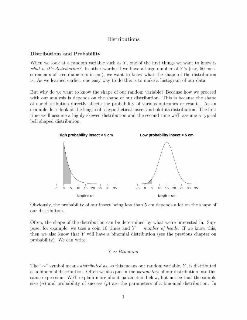
But why do we want to know the shape of our random variable? Because how we proceedwith our analysis is depends on the shape of our distribution. This is because the shapeof our distribution directly affects the probability of various outcomes or results. As anexample, let’s look at the length of a hypothetical insect and plot its distribution. The firsttime we’ll assume a highly skewed distribution and the second time we’ll assume a typicalbell shaped distribution.

High probability insect < 5 cm

length in cm

−5 0 5 10 15 20 25 30 35

Low probability insect < 5 cm

length in cm

−5 0 5 10 15 20 25 30 35

Obviously, the probability of our insect being less than 5 cm depends a lot on the shape ofour distribution.

Often, the shape of the distribution can be determined by what we’re interested in. Sup-pose, for example, we toss a coin 10 times and Y = number of heads. If we know this,then we also know that Y will have a binomial distribution (see the previous chapter onprobability). We can write:

Y ∼ Binomial

The ”∼” symbol means distributed as, so this means our random variable, Y , is distributedas a binomial distribution. Often we also put in the parameters of our distribution into thissame expression. We’ll explain more about parameters below, but notice that the samplesize (n) and probability of success (p) are the parameters of a binomial distribution. In

1

Distributions 2

this case we have n = 10 and p = 0.5, so we can re-write our expression as follows:

Y ∼ Binomial(10, 0.5)

or, simpler:

Y ∼ B(10, 0.5)

Finally, we should mention that this is the theoretical distribution of our random variable(Y ). If we actually toss a coin 10 times and to this many, many times (say 1,000 times),then our actual distribution may eventually look like our theoretical distribution (if ourcoin is fair).

More on the binomial distribution

Let’s briefly review the binomial distribution that we first introduced when we looked atprobability. Here’s the equation again:(

n

y

)py(1− p)n−y

So what makes this a distribution? Several reasons (this breakdown may vary a bit indifferent texts):

1. We can use this equation to calculate the probability of any (or all) possible out-come(s).

2. All possible outcomes add up to 1 (the probability of something happening is 1).

3. The actual shape of the distribution is determined by the parameters of the distribu-tion.

Let’s explain these in a bit more detail using our coin example (10 tosses with a faircoin). We can use our binomial distribution formula to calculate all possible outcomes. Forexample, the probability of 0 tails in 10 tosses would be:(

10

0

)0.50(1− 0.5)10−0 = 0.00098

The probability of 1 tail in 10 tosses would be:(10

1

)0.51(1− 0.5)10−1 = 0.00977

The probability of 2 tails in 10 tosses (which, incidentally, is equal to the probability of 8tails in 10 tosses (only true if p = 0.5), which we calculated in the chapter on probability)

©2017 Arndt F. Laemmerzahl

Distributions 3

would be: (10

2

)0.52(1− 0.5)10−2 = 0.04395

We could go on and do all 11 possible outcomes, but let’s just list the answers in a table:

Heads Tails Probability10 0 0.000989 1 0.009778 2 0.043957 3 0.117196 4 0.205085 5 0.246094 6 0.205083 7 0.117192 8 0.043951 9 0.009770 10 0.00098

Sum: 1.00000

A summary like this that lists all possible outcomes can be very useful. For example, wecan now easily calculate the probability that Y = 0, 1, or 2 heads:

Pr{0 ≤ Y ≤ 2} = 0.00098 + 0.00977 + 0.04395 = 0.05470

Also notice that all possible outcomes add to 1.0:

PrPr{0 ≤ Y ≤ 10} = 1.0

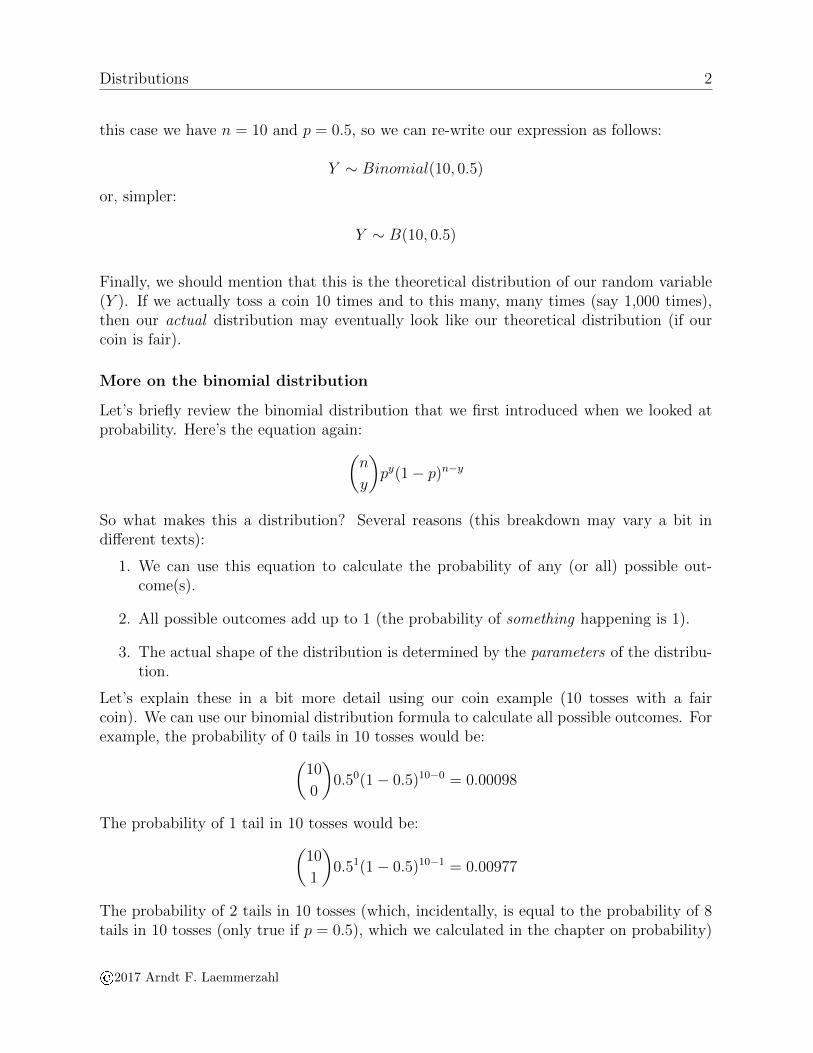
This is a very important point that should be obvious: if we toss a coin, something has tohappen. Since the above table lists every possible outcome, these outcomes add to 1.So let’s take a look at our (theoretical) distribution and see what it looks like. To do this,we simply plot each probability as the height on a bar graph:


Distributions 4

0 1 2 3 4 5 6 7 8 9 10

Number of heads

Pro

babi

lity

0.00

0.05

0.10

0.15

0.20

0.25

0.30

This gives us a visual representation of the distribution of our random variable.

noindent So what about the parameters? Parameters determine what our distributionlooks like. In our coin tossing example our parameters were n = 10, and p = 0.5. So whathappens if we change our parameters? The shape of our distribution changes.

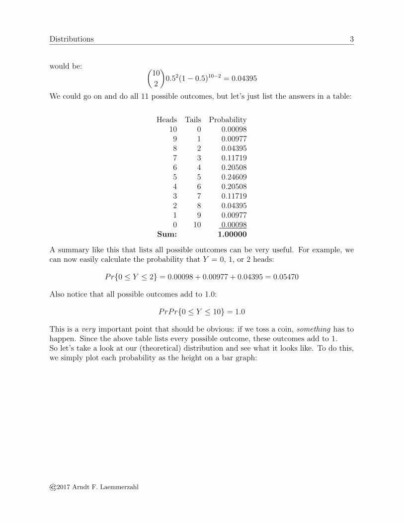
Suppose we had an unfair coin. Somehow we’ve managed to rig our coin so it comesup heads only 20% of the time. That implies our p = 0.2. Now (mostly because we don’twant to plot 11 outcomes again), let’s assume we toss it three times (n =3). What doesthis do to the shape of our distribution? Let’s calculate all possible outcomes first, justlike we did above (remember Y = number of heads):

Y Probability0 0.5121 0.3842 0.0963 0.008

Sum: 1.00000


Distributions 5

If you don’t know how we got the probabilities in the table above, you should review theearlier parts of this chapter. But let’s plot this just like we did before:

0 1 2 3

Number of heads

Pro

babi

lity

0.0

0.1

0.2

0.3

0.4

0.5

0.6

And we notice that the shape (and number of bars) has changed considerably. In otherwords, the parameters determine what our distribution looks like!

Summarizing distributions so far

Based on what we learned about the binomial distribution, we can now remind ourselvesof two properties of distributions:

1. The shape of a distribution varies based on the parameters.

2. All possible outcomes must add up to 1.

Let’s investigate property (2.) a little more. If we have a discrete distribution (if Y isdiscrete), then it’s easy to see how to add up all possible outcomes. Again, using thebinomial as an example, what we are saying is:

n∑y=0

(n

y

)py(1− p)n−y = 1.0

This principle is not true just for the binomial, but for any distribution. If our distributionis discrete, we can just rewrite our equation as follows:

n∑y=0

f(y) = 1.0

Where f(y) is our discrete distribution (e.g., the binomial).

But what do we do if our distribution is continuous? How can we possible add up all


Distributions 6

possible values? Let’s think about this for a moment by illustrating a simple probabilityfor a continuous variable. We’ll let Y = height of a woman. So let’s figure out the following:

Pr{Y = 65 inches} =??

This might seem like a simple calculation (and it is), but the answer isn’t obvious. Let’srewrite this to make the answer a bit more obvious:

Pr{Y = 65 inches} = Pr{Y = 65.00000000000000000000000000... inches} = 0.0

In other words, no one is exactly 65 inches tall. So how do we add up all possible outcomes,if the probability of any particular event is 0? Unfortunately, the answer requires calculus.

You are not responsible for calculus, but let’s investigate this just a bit further. Usingcalculus, mathematicians (and statisticians!) can add up a bunch of infinitely small thingslike the probability of someone being between 65 and 66 inches (the probability of any oneoutcome is 0, but amazingly we can still add these up!). What we are saying is somethinglike the following: ∫ ∞

−∞f(y)dy = 1.0

Where this time f(y) represents our continuous distribution. Note that if you replace the∫symbol with the

∑symbol and ignore the dy, you essentially have the same thing we

did above. In fact, historically the∫

symbol means “sum”.

So to summarize, and temporarily get away from calculus, we can use calculus to addup a sequence of infinitely small things. If we use this to add up all possible outcomes, wemust get 1. Or, as a simple example, the probability that a particular woman has a height(any height) is 1.0 (she must have a height, or she wouldn’t exist). So any distribution,discrete or continuous will give us 1 if we add up all possible outcomes.

Introducing the normal distribution

The normal distribution is without a doubt the most important distribution in statistics.Some of the reasons for that won’t be apparent for a while, but have to do with the prop-erties of random variables.

As an aside, the normal distribution is also knows as the Gaussian distributionafter Carl Friedrich Gauß (1777 - 1855), who did a lot of work with it. Gauß wasone of the most famous mathematicians of all time and made major contributionsto number theory, statistics, geometry, linear algebra and many other fields. Infact, the Germans used his picture on the 10DM bill and even put the equation(yes, the equation!) for the normal (or Gaussian) distribution on the bill rightnext to his picture (the DM was the old German currency before the introductionof the Euro). If you’re interested in Gauß, you should check out his page onWikipedia.


Distributions 7

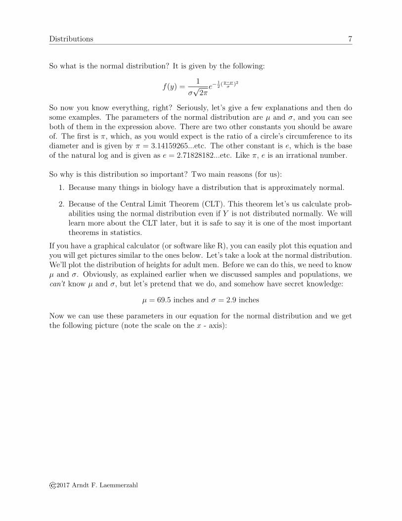
So what is the normal distribution? It is given by the following:

f(y) =1

σ√

2πe−

12( y−µσ

)2

So now you know everything, right? Seriously, let’s give a few explanations and then dosome examples. The parameters of the normal distribution are µ and σ, and you can seeboth of them in the expression above. There are two other constants you should be awareof. The first is π, which, as you would expect is the ratio of a circle’s circumference to itsdiameter and is given by π = 3.14159265...etc. The other constant is e, which is the baseof the natural log and is given as e = 2.71828182...etc. Like π, e is an irrational number.

So why is this distribution so important? Two main reasons (for us):

1. Because many things in biology have a distribution that is approximately normal.

2. Because of the Central Limit Theorem (CLT). This theorem let’s us calculate prob-abilities using the normal distribution even if Y is not distributed normally. We willlearn more about the CLT later, but it is safe to say it is one of the most importanttheorems in statistics.

If you have a graphical calculator (or software like R), you can easily plot this equation andyou will get pictures similar to the ones below. Let’s take a look at the normal distribution.We’ll plot the distribution of heights for adult men. Before we can do this, we need to knowµ and σ. Obviously, as explained earlier when we discussed samples and populations, wecan’t know µ and σ, but let’s pretend that we do, and somehow have secret knowledge:

µ = 69.5 inches and σ = 2.9 inches

Now we can use these parameters in our equation for the normal distribution and we getthe following picture (note the scale on the x - axis):


Distributions 8

Height for men in inches

57.9 60.8 63.7 66.6 69.5 72.4 75.3 78.2 81.1

We notice that the curve reaches its peak (maximum value) at µ = 69.5. Also notice thatthe curve changes direction (has an inflection point) at µ± σ, or in this case at 69.5± 2.9.Finally, notice that the ends of the curve go from −∞ to +∞.

Let’s try this again, but this time we’ll look at the number of eggs laid by Gray TreeFrogs (Hyla versicolor). Again, let’s pretend we have secret knowledge and know thatµ = 1, 800 and σ = 250:


Distributions 9

Number of eggs laid

1200 1350 1500 1650 1800 1950 2100 2250 2400

This plot looks identical to the one for the height of men (are they the same?). Let’s makesome comments on the normal distribution.

First, if you look at the scale of the two normal curves, they are obviously not the same.The first is centered at 69.5, the second at 1,800. Also, the first is considerably less widethan the second. Let’s visualize this by plotting them both on the same graph:


Distributions 10

Y

0 250 500 750 1000 1250 1500 1750 2000 2250

Normal curve for frog eggs

Normal curve for height of men

As you can see, the two normal curves actually look rather different if drawn to the samescale. As should be obvious, the parameters of the normal curve are µ and σ: the twonumbers we changed for the two normal curves above.

Conveniently, the mean and standard deviation of a normal curve are actually the param-eters (µ and σ). The mean (µ) determines the exact location of the normal distribution onthe x− axis. The standard deviation (σ) determines how spread out the normal distribu-tion is (this should be obvious looking at the graph above).

So how does this help us in calculating probabilities? As implied above, the area un-der the normal curve has to add to 1 (this is a fundamental property of a distibution).What we are saying (using calculus) is:∫ ∞

−∞

1

σ√

2πe−

12( y−µσ

)2dy = 1.0

While we can’t use a continuous distributionlie this to calculate the probability that Y isequal to any one value, we can use it to calculate the probability that Y is greater or lessthan any particular value. For example, we can calculate the probability that a particulargray tree frog lays less than 1700 eggs:

Pr{Y < 1700 eggs}


Distributions 11

If you do know calculus, you might think the way to calculate this probablity is as follows:∫ 1700

−∞

1

250√

2πe−

12( y−1800

250)2dy

Where we plugged in σ = 250 and µ = 1800. Unfortunately, this equation isn’t solveableanalytically, so we need to resort to other techniques. What we do is use a table to lookup this probability (or letting R do this for us).

But before we can do this, we have one more problem to solve. We illustrated two differentnormal curves above. How many different normal curves are there? If you think about thisfor a minute, we can’t possibly make a table for every possible normal curve.

Instead, we will use just one normal curve to look up our probilities and convert thevalues of our curve to this normal curve (see below). The curve we choose is called thestandard normal curve and has µ = 0 and σ = 1.

Standard normal curve (Z)

−4 −3 −2 −1 0 1 2 3 4−4 −3 −2 −1 0 1 2 3 4

Note that we also use Z instead of Y for this distribution. We say Z ∼ N(0, 1).

So how do we use this to calculate probabilities? The values for this curve are tabu-lated in the standard normal table. Here’s how to use it:

Suppose we want to find the probability that Z is greater than 1.73 (we want Pr{Z >1.73}). First let’s draw a picture of what we want:


Distributions 12

Total area = 1.0

Z

−4 −3 −2 −1 0 1 2 3 4

Area for z greater than 1.73

The probability (which is the area above) should be fairly small. Our normal distributiontable gives the you the area less than a particular value of Z. The side gives the first twodigits of z, and the top gives the third digit of z. So to get the area less than Z = 1.73(remember we want greater than) we go into the table and look for ”1.7“ on the side of thetable and 0.03 across the top of the table. Then we pick out our area (= probability) andget 0.9582. In other words:

Pr{Z < 1.73} = 0.9482

We’re almost done. If you remember, we want Pr{Z < 1.73}, not Pr{Z < 1.73}. Sincethe area under the curve is 1, we can simply subtract to get our answer:

Pr{Z > 1.73} = 1− Pr{Z < 1.73} = 1− 0.9582 = 0.0418

And we have our answer.


Distributions 13

There is a slightly easier way to do this, particulary once you get comfortable withthis idea. We notice that the curve is completely symmetrical around 0. We cantake advantage of this:

1. Change the sign of the z we’re interested in. In our example we would use-1.73 instead of 1.73.

2. Change the inequality and then simply look up Pr{Z < −1.73} in thenormal table.

And we find that Pr{Z < −1.73} = 0.0418 (= Pr{Z > 1.73})

This always works due to the symmetry of the normal curve, which is whysome text will only give you one half of the normal table. If you find thisconfusing, just stick with the method outlined above.

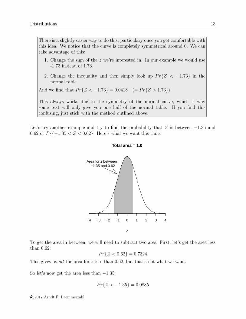
Let’s try another example and try to find the probability that Z is between −1.35 and0.62 or Pr{−1.35 < Z < 0.62}. Here’s what we want this time:

Total area = 1.0

Z

−4 −3 −2 −1 0 1 2 3 4

Area for z between −1.35 and 0.62

To get the area in between, we will need to subtract two ares. First, let’s get the area lessthan 0.62:

Pr{Z < 0.62} = 0.7324

This gives us all the area for z less than 0.62, but that’s not what we want.

So let’s now get the area less than −1.35:

Pr{Z < −1.35} = 0.0885


Distributions 14

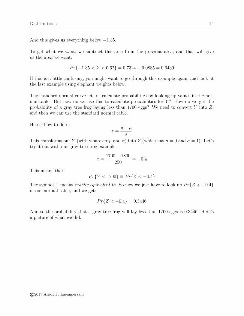
And this gives us everything below −1.35.

To get what we want, we subtract this area from the previous area, and that will giveus the area we want:

Pr{−1.35 < Z < 0.62} = 0.7324− 0.0885 = 0.6439

If this is a little confusing, you might want to go through this example again, and look atthe last example using elephant weights below.

The standard normal curve lets us calculate probabilities by looking up values in the nor-mal table. But how do we use this to calculate probabilities for Y ? How do we get theprobability of a gray tree frog laying less than 1700 eggs? We need to convert Y into Z,and then we can use the standard normal table.

Here’s how to do it:

z =y − µσ

This transforms our Y (with whatever µ and σ) into Z (which has µ = 0 and σ = 1). Let’stry it out with our gray tree frog example:

z =1700− 1800

250= −0.4

This means that:Pr{Y < 1700} ≡ Pr{Z < −0.4}

The symbol ≡ means exactly equivalent to. So now we just have to look up Pr{Z < −0.4}in our normal table, and we get:

Pr{Z < −0.4} = 0.3446

And so the probability that a gray tree frog will lay less than 1700 eggs is 0.3446. Here’sa picture of what we did:


Distributions 15

Total area = 1.0

Number of eggs

800 1300 1800 2300 2800

Total area = 1.0

Standard normal

−4 −2 0 1 2 3 4

The area in the two graphs above is identical, which is why we can use the standard normaldistribution to look up our probablities.

Let’s try a few more examples using African Elephants (Loxodonta africana). Somehow weknow that for male elephants, µ = 7, 400kg and σ = 500kg.

Example 1 : We want to find the probability an individual elephant weight less than6,500kg:First, let’s draw a picture of what we want using elephant weights:

Total area = 1.0

Weight of male elephant in kg

5400 6400 7400 8400 9400


Distributions 16

Now let’s convert our Y to Z:

z =y − µσ

=6, 500− 7, 400

500= −1.8

And we can look at what we want on the standard normal curve (notice the areas areidentical, as they should be!):

Total area = 1.0

Standard normal

−4 −3 −2 −1 0 1 2 3 4

Finally, we look up −1.8 inour table and get 0.0359. So we can conclude:

Pr{Y < 6, 500} = Pr{Z < −1.84} = 0.0359

Example 2 : We want to find the probability an individual elephant weight more than8,000kg. Again, let’s start with a picture (only one this time):


Distributions 17

Total area = 1.0


5400 6400 7400 8400 9400

Now let’s convert our Y to Z as in the last example:

z =y − µσ

=8, 000− 7, 400

500= 1.2

We look up Pr{Z > 1.2} = 0.8849, and finally we do:

Pr{Y > 8, 000} = Pr{Z > 1.2} = 1− 0.8849 = 0.1151

(Or we could have noted that Pr{Z > 1.2} = Pr{Z < −1.2} and looked up Pr{Z <−1.2} = 0.1151).

Example 3 : Finally, let’s get the probability an individual elephant weight more between8,000kg and 8,500 kg. Here’s our picture this time:


Distributions 18

Total area = 1.0


5400 6400 7400 8400 9400

This time we need two values of Z:

z1 =8, 000− 7, 400

500= 1.2

z2 =8, 500− 7, 400

500= 2.2

This implies that Pr{8, 000 < 8, 500} = Pr{1.2 < Z < 2.2}. To get our answer, we lookup Pr{Z < 2.2} = 0.9861. This gives us all of the area less than 2.2. However, we don’twant all of this area, we want the area between 1.2 and 2.2, so we need to subtract thearea less than 1.2. In other words we look up Pr{Z < 1.2} = 0.8849. Now we can do oursubtraction and conclude:

Pr{8, 000 < 8, 500} = Pr{1.2 < Z < 2.2} = 0.9861− 0.9949 = 0.1012

Now that we have figured out how to calculate (look up) probabilities using the normaldistribution, we need to do one more thing. Suppose we have a particular probability inmind, and want to figure out the value of Y that goes with that probability? This maysound a bit confusing, so let’s illustrate this using our elephants.

I want to know the weight that corresponds to 90% of my elephants, or to put it an-other way, 90% of elephants weigh less than ? We want to fill in that blank. If we putthis into a probability statement, here is what we’re after:

Pr{Y < y} = 0.90


Distributions 19

We want to find the y that makes the above statement true. What value of y is equivalentto 90% of the area? We also call these values percentiles. For example:

The 90th percentile has 90% of the values of Y below y.

The 64th percentile has 64% of the values of Y below y.

(This might be a good time to remember that Y is a random variable and y is anactual value).

Let’s motivate this a bit further by looking at an example from academic testing. Manycolleges require students to take the SAT or ACT before they are admitted. These tests(supposedly) measure how well prepared you are for college level work. In addition to ascore, these tests will also give you a percentile. These percentiles tell you how you com-pared to everyone else taking the same exam.

For example, you score 73% on a part of the test. This means you did better than 73% ofthe people taking this test (for that part). Your score, whatever it was, corresponds to the73rd percentile.

Many testing agencies use percentiles because it is informative and also makes variationsin the test from one version to the next comparable. In other words, if you scored in the73rd percentile this year and in the 73rd percentile last year, your performance was similarcompared to everyone else, regardless of what your scores were (your scores could be dif-ferent, but your percentiles are the same).

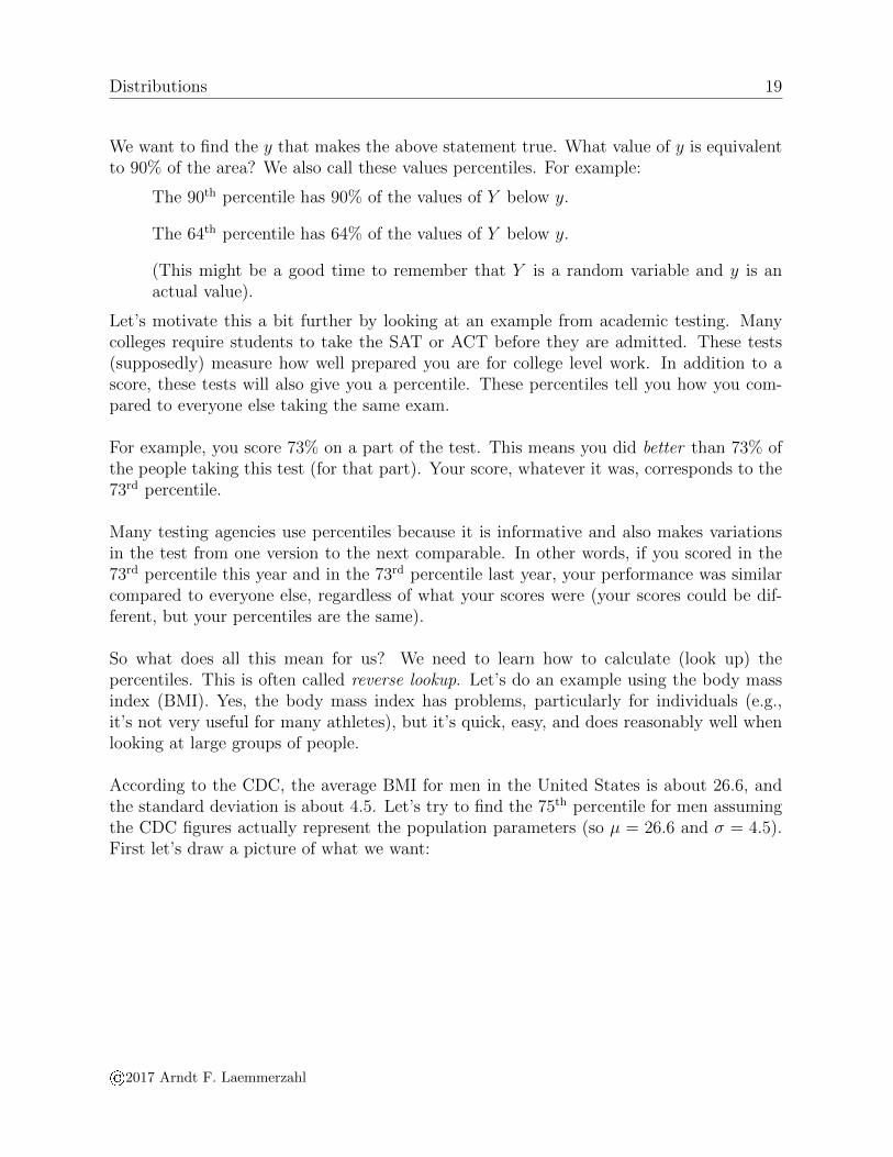
So what does all this mean for us? We need to learn how to calculate (look up) thepercentiles. This is often called reverse lookup. Let’s do an example using the body massindex (BMI). Yes, the body mass index has problems, particularly for individuals (e.g.,it’s not very useful for many athletes), but it’s quick, easy, and does reasonably well whenlooking at large groups of people.

According to the CDC, the average BMI for men in the United States is about 26.6, andthe standard deviation is about 4.5. Let’s try to find the 75th percentile for men assumingthe CDC figures actually represent the population parameters (so µ = 26.6 and σ = 4.5).First let’s draw a picture of what we want:


Distributions 20

Total area = 1.0

Body Mass Index

8.6 13.1 22.1 31.1 40.1

Area = 75%

We want this y

So here is how to do it. We remember that our normal distribution table gives us the area(= probability) below the number (z) that we look up. Normally we would use our z tolook up the probability. Now we do things backwards. In other words, Now we want tofind z in Pr{Z < z} = 0.75 (up until now we calculate z and look up the probability (0.75,in this case)).

To do this, We go into the body of the table (not along the sides or top) and look forthe number that’s closest to 0.75. This turns out to be 0.7486 (a little closer to 0.75 thanthe next number, 0.7517). Now that we have found 0.7486, we look up z: we move from0.7486 to the side and fine 0.6, we go to the top and find 0.07, so we now z = 0.67. Wenow know that:

Pr{Z < 0.67} ≈ 0.75

We will not worry about extrapolation in our class - instead we will just get the closestnumber.

Now all we need to do is to convert our z back to y. We just rearrange our equationfor z and get:

z =y − µσ

=⇒ y = zσ + µ

So we can do:y = 0.67(4.5) + 26.6 = 29.615

And we can say that the 75th percentile for BMI in men is 29.615, or 75% of men have aBMI that is less than 29.615.


Distributions 21

Finally, we should remember that statistics is about more than just numbers and thinkabout our results just a bit. If we realize that a BMI of 25 or higher is considered over-weight, and 30 or higher is obese, what do these numbers tell us about men in the U.S.?


distributions - george mason universitymason.gmu.edu/~alaemmer/bio214/distributions.pdf ·...

Documents