distributions of error correction tests for...

Econometrics Journal(2002), volume5, pp. 285–318.

Distributions of error correction tests for cointegration

NEIL R. ERICSSON† AND JAMES G. MACK INNON‡

†Stop 20, Division of International Finance, Federal Reserve Board, 2000 C Street, NW,Washington, DC 20551, USAE-mail:[email protected]

‡Department of Economics, Queen’s University, Kingston, Ontario, Canada K7L 3N6E-mail:[email protected];

Homepage:www.econ.queensu.ca/faculty/mackinnon

Received: January 2000

Summary This paper provides densities and finite sample critical values for the single-equation error correction statistic for testing cointegration. Graphs and response surfaces sum-marize extensive Monte Carlo simulations and highlight simple dependencies of the statistic’squantiles on the number of variables in the error correction model, the choice of deterministiccomponents, and the sample size. The response surfaces provide a convenient way for calcu-lating finite sample critical values at standard levels; and a computer program, freely availableover the Internet, can be used to calculate both critical values andp-values. Two empiricalapplications illustrate these tools.

Keywords: Cointegration, Critical value, Distribution function, Error correction, MonteCarlo, Response surface.

1. INTRODUCTION

Three general approaches are widely used for testing whether or not non-stationary economictime series are cointegrated: single-equation static regressions, due to Engle and Granger (1987);vector autoregressions, as formulated by Johansen (1988, 1995); and single-equation conditionalerror correction models, initially proposed by Phillips (1954) and further developed by Sargan(1964). While all three have their advantages and disadvantages, testing for cointegration withany of these approaches requires non-standard critical values, which are usually calculated byMonte Carlo simulation. Engle and Granger (1987) tabulate a limited set of critical values fortheir procedure. MacKinnon (1991) derives a more extensive set with finite sample correctionsbased on response surfaces, and MacKinnon (1996) provides a computer program to calculatecritical values for Engle and Granger’s test at any desired level. Johansen (1988), Johansen andJuselius (1990), and Osterwald-Lenum (1992) include critical values for the Johansen proce-dure under typical assumptions about deterministic terms and the number of stochastic variables.Johansen (1995), Doornik (1998), and MacKinnonet al.(1999) provide more accurate estimatesof these critical values, with the last of these papers also providing computer programs to calcu-late critical values andp-values.

c© Royal Economic Society 2002. Published by Blackwell Publishers Ltd, 108 Cowley Road, Oxford OX4 1JF, UK and 350 Main Street,Malden, MA, 02148, USA.

286 Neil R. Ericsson and James G. MacKinnon

By contrast, critical values for the single-equation error correction procedure are scant, per-haps because error correction models substantially predate the literature on cointegration. Baner-jeeet al. (1993) tabulate critical values for an error correction model with two variables at threesample sizes; and Banerjeeet al. (1998) list critical values for models with two through six vari-ables at five sample sizes. Harboet al.(1998), MacKinnonet al.(1999), and Pesaranet al.(2000)list asymptotic critical values for a related but distinct procedure for single- and multiple-equationerror correction models.

The current paper addresses this dearth by providing an extensive set of cointegration criticalvalues for the single-equation error correction model. These critical values include finite sampleadjustments similar to those in MacKinnon (1991, 1996) for the Engle–Granger (EG) proce-dure, they are very accurate numerically and are easy to use in practice, and they encompassand supersede comparable results in Banerjeeet al. (1993) and Banerjeeet al. (1998). We alsoprovide a freely available Excel spreadsheet and a Fortran program (the latter being similar to theone in MacKinnon (1996) for the EG procedure) that compute both critical values andp-valuesfor the error correction statistic. As the articles in Banerjee and Hendry (1996), Ericsson (1998),and Lutkepohl and Wolters (1998)inter alia highlight, conditional error correction models areubiquitous empirically, so these tools for calculating critical values andp-values should be ofimmediate and widespread use to the empirical modeler. Finally, general distributional proper-ties are of considerable interest. Accurate numerical approximations to the entire distributionof the error correction statistic are calculated herein and offer insights into the nature of thatstatistic, particularly relative to the Dickey–Fuller and EG statistics. Graphs highlight the errorcorrection statistic’s properties and relationships, and show for the first time what many of its var-ious distributions look like. Throughout, the focus is on testing for cointegration, rather than onthe complementary task of estimating the cointegrating vectors, assuming a given cointegrationrank.

This paper is organized as follows. Section 2 sets the backdrop by considering the threecommon procedures and their relationships to each other. Section 3 outlines the structure of theMonte Carlo analysis for calculating the distributional properties of the cointegration test statisticbased on the single-equation error correction model. Section 4 presents the Monte Carlo results,which include densities and finite sample critical values. Section 5 applies the finite sample crit-ical values derived in Section 4 and the computer program for calculatingp-values to empiricalerror correction models of UK narrow money demand from Hendry and Ericsson (1991) and ofUS federal government debt from Hamilton and Flavin (1986). Section 6 concludes.

2. AN OVERVIEW OF THREE TEST PROCEDURES

This paper focuses on finite sample inference about cointegration in a single-equation condi-tional error correction model (ECM).1 To motivate the use of conditional ECMs, this sectiondescribes the analytics of and inferential methods for the three common approaches for test-ing cointegration: the Johansen procedure (Section 2.1), the conditional ECM (Section 2.2), andthe EG procedure (Section 2.3). Differences between the three approaches turn on their variousassumptions about dynamics and exogeneity (Section 2.4).

1Strictly speaking, the models examined herein are equilibrium correction models; see Hendry and Doornik (2001,p. 144).

c© Royal Economic Society 2002

Distributions of error correction tests for cointegration 287

2.1. The Johansen procedure

Johansen (1988, 1995) derives maximum likelihood procedures for testing for cointegration in afinite-order Gaussian vector autoregression (VAR). That system is:

xt =

∑i =1

πi xt−i + 8Dt + εt , εt ∼ I N (0, �), t = 1, . . . , T, (1)

wherext is a vector ofk variables at timet ; πi is ak×k matrix of coefficients on thei th lag ofxt ;` is the maximal lag length;8 is ak × d matrix of coefficients onDt , a vector ofd deterministicvariables (such as a constant term and a trend);εt is a vector ofk unobserved, sequentiallyindependent, jointly normal errors with mean zero and (constant) covariance matrix�; andT isthe number of observations. Throughout,x is restricted to be (at most) integrated of order one,denoted I(1), where an I(j ) variable requiresj th differencing to make it stationary.

The VAR in (1) may be rewritten as a vector error correction model:

1xt = πxt−1 +

`−1∑i =1

0i 1xt−i + 8Dt + εt , εt ∼ I N (0, �), (2)

whereπ and0i are:

π =

(∑i =1

πi

)− Ik, (3)

0i = −(πi +1 + · · · + π`), i = 1, . . . , ` − 1, (4)

Ik is the identity matrix of dimensionk, and1 is the difference operator.2 For any specifiednumber of cointegrating vectorsr (0 ≤ r ≤ k), the matrixπ is of (potentially reduced) rankrand may be rewritten asαβ ′, whereα andβ arek×r matrices of full rank. By substitution, (2) is:

1xt = αβ ′xt−1 +

`−1∑i =1

0i 1xt−i + 8Dt + εt , εt ∼ I N (0, �), (5)

whereβ is the matrix of cointegrating vectors, andα is the matrix of adjustment coefficients(equivalently, the loading matrix).

Johansen (1988, 1995) derives two maximum likelihood statistics for testing the rank ofπ

in (2) and hence for testing the number of cointegrating vectors in (2). Critical values appearin Johansen (1988, Table 1) for a VAR with no deterministic components, in Johansen andJuselius (1990, Tables A1–A3) for VARs with a constant term, and in Osterwald-Lenum (1992)and Johansen (1995, Ch. 15) for VARs with no deterministic components, with a constant termonly, and with a constant term and a linear trend. Doornik (1998) derives a convenient approxi-mation to the maximum likelihood statistics’ distributions using the Gamma distribution, andMacKinnonet al. (1999) provide computer programs to calculate critical values andp-valuesfor the Johansen procedure.

2The difference operator1 is defined as(1 − L), where the lag operatorL shifts a variable one period into the past.Hence, forxt , Lxt = xt−1 and so1xt = xt − xt−1. More generally,1i

j xt = (1 − L j )i xt for positive integersi and j .If i or j is not explicit, it is taken to be unity.



2.2. Single-equation conditional error correction models

Without loss of generality, the VAR in (1) can be factorized into a pair of conditional and marginalmodels. If the marginal variables are weakly exogenous for the cointegrating vectorsβ, theninference about cointegration using the conditional model alone can be made without loss ofinformation relative to inference using the full system (the VAR); see Johansen (1992a,b). Thissubsection derives asingle-equationconditional model from the VAR and delineates two relatedapproaches for conducting such inferences about cointegration from that conditional model. Thesecond of those approaches is the focus of the Monte Carlo analysis in Sections 3 and 4 and ofthe empirical analysis in Section 5.

For expositional clarity, assume that (1) is a first-order VAR with no deterministic compo-nents. Its explicit representation as the vector error correction model (2) is:

1yt = π(11)yt−1 + π(12)zt−1 + ε1t (6)

1zt = π(21)yt−1 + π(22)zt−1 + ε2t , (7)

wherex′t = (yt , z′

t ), yt is a scalar endogenous variable,zt is a(k − 1) × 1 vector of potentiallyweakly exogenous variables,π is partitioned conformably toxt as{π(i j )}, andε′

t = (ε1t , ε′

2t ).From (5), equations (6) and (7) may be written as:

1yt = α1β′xt−1 + ε1t (8)

1zt = α2β′xt−1 + ε2t , (9)

whereα′= (α1, α

′

2). Equations (8) and (9) may always be factorized into the conditional distri-bution of yt given zt and lags on both variables, and the marginal distribution ofzt (also givenlags on both variables):

1yt = γ ′

01zt + γ1β′xt−1 + ν1t (10)

1zt = α2β′xt−1 + ε2t , (11)

whereγ ′

0 = �12�−122 , γ1 = α1 − �12�

−122 α2, ν1t = ε1t − �12�

−122 ε2t , the expectationE(ν1tε2t )

is zero (by construction), and the error covariance matrix� in (1) is {�i j }. Equivalently, theerrorε1t in (8) may be partitioned into two uncorrelated components asε1t = ν1t + γ ′

0ε2t , andthenε2t is substituted out to obtain (10).

The variablezt is weakly exogenous forβ if and only if α2 = 0 in (11), in which case (10)and (11) become:

1yt = γ ′

01zt + γ1β′xt−1 + ν1t (12)

1zt = ε2t , (13)

whereγ1 = α1. The test ofzt being weakly exogenous forβ is thus a test ofα2 = 0; see Johansen(1992a).

If α2 = 0, the conditional ECM (12) by itself is sufficient for inference aboutβ that is with-out loss of information relative to inference from (10) and (11) together. Two distinct approacheshave evolved for testing cointegration in the conditional ECM (12): one is due to Harboet al.(1998), and the other originates from the literature on ECMs. The current paper analyzes thesecond approach, and clarifying the distinction between the two approaches is central to under-standing their respective properties.



Harbo et al. (1998) derive the likelihood ratio statistic for testing cointegrating rank in aconditional subsystem obtained from a Gaussian VAR when the marginal variables are weaklyexogenous forβ. For a single-equation conditional model such as (12), the null hypothesis beingtested isγ1β

′= 0, i.e. that the cointegrating rank forx is zero. The alternative hypothesis is that

γ1β′6= 0, implying thatx has a cointegrating vectorβ with at least one non-zero element.

The second approach stems from the literature on error correction models and is based ontransformations of (12), with an auxiliary assumption about the nature ofx’s cointegration.Specifically, the conditional ECM (12) can be motivated as a reparameterization of the condi-tional autoregressive distributed lag (ADL) model; see Davidsonet al. (1978) and Hendryet al.(1984) inter alia. Data transformations imply reparameterizations, and two transformations areof particular interest:

differencing: µ1xt + µ2xt−1 → µ11xt + (µ1 + µ2)xt−1differentials: µ1yt + µ2zt → µ1(yt − zt ) + (µ1 + µ2)zt ,

for arbitrary coefficientsµ1 andµ2. Repeatedly applying these two transformations re-arrangesa conditional ADL into the conditional ECM (12):

yt = λ′

0zt + λ′

1zt−1 + λ2yt−1 + ν1t (14)

yt = γ ′

01zt + λ′

3zt−1 + λ2yt−1 + ν1t (15)

1yt = γ ′

01zt + λ′

3zt−1 + γ1yt−1 + ν1t (16)

1yt = γ ′

01zt + γ1(yt−1 − δ′zt−1) + ν1t (17)

1yt = γ ′

01zt + γ1β′xt−1 + ν1t , (18)

whereλ0, λ1, λ2, λ3, andδ are various coefficients; and the cointegrating vectorβ has beennormalized on its first coefficient (i.e. fory) such thatβ ′

= (1, −δ′). In practice, significancetesting of the error correction term typically has been based on thet-ratio forγ1 in (16), not (17)or (18). This is the ‘PcGive unit root test’ in Hendry (1989, p. 149) and Hendry and Doornik(2001, p. 256), which here is denoted the ECM statistic.

When interpreted as a test for cointegration ofx, this approach requires an additional assump-tion: namely, that the variables inz are not cointegrated among themselves. Thus,γ1 = 0 in (16)implies (and is implied by) a lack of cointegration betweeny andz, whereasγ1 < 0 impliescointegration. Thet-ratio based upon the least squares estimator ofγ1 in (16) is the ECM statis-tic analyzed in Sections 3–5. Thatt-ratio is denotedκd(k), whered indicates the deterministiccomponents included in the ECM, or the number of such deterministic components, dependingupon the context; andk is the total number of variables inx (not to be confused with the num-ber of regressors in the ECM). Thist-ratio is used to test the null hypothesis thatγ1 = 0, i.e.that y andz arenot cointegrated. If weak exogeneity does not hold, critical values generally areaffected; see Hendry (1995).

Camposet al. (1996) and Banerjeeet al. (1998) derive the asymptotic distribution ofκd(k)

under the null hypothesis of no cointegration:

κd(k) ⇒

(∫B2

v

)−1/2 ∫Bv d Bv, (19)

where Bv and Bε are the standardized Wiener processes corresponding tov1t and ε2t , Bv is

Bv −(∫

Bε Bv

)′ (∫Bε B′

ε

)−1Bε, ‘⇒’ denotes weak convergence of the associated probability



measures asT → ∞, strong exogeneity ofz with respect toα andβ is assumed, and the ECMhas no deterministic terms. If the ECM includes deterministic terms, the asymptotic distributionof κd(k) is of the same form as in (19), but with the Wiener processes replaced by the correspond-ing Brownian bridges. Johansen (1995, Ch. 11.2) develops analogous algebra for the Johansenmaximum likelihood statistic when the VAR has deterministic terms.

Kiviet and Phillips (1992) and Banerjeeet al. (1998) discuss similarity forκd(k). Notably,the asymptotic distribution in (19) depends onk andd, but not on the short-run coefficients inthe ECM. That is,κd(k) is asymptotically similar with respect toγ0, and also with respect tocoefficients on any lags of1x in the ECM, provided that those parameters lie within the spacesatisfying the I(1) conditions forx. The statisticκd(k) is exactlysimilar with respect to theconstant term if the estimated ECM includes a constant term and a linear trend, and with respectto the constant term and the linear trend’s coefficient if the estimated ECM includes a constantterm, a linear trend, and a quadratic trend. Following Johansen (1995, p. 84), seasonal dummieswith a constant term may affect the finite sample (but not asymptotic) distribution. Likewise, thechoice of a fixed lag lengthaffects the finite sample (but not asymptotic) distribution, provided` is large enough to avoid mis-specification; see Banerjeeet al. (1998, Section 5).

To summarize, the ECM statisticκd(k) is designed to detect cointegration involvingy in theconditional model (12). The procedure in Harboet al. (1998) is designed to detect any coin-tegration inx in the conditional model (12), where that cointegration may includey or it maybe restricted toz alone. While both statistics derive from conditional models, the two statisticsare testing different hypotheses. They have different distributions—even asymptotically—and sorequire separate tabulation.

Harboet al. (1998, Tables 2–4) present asymptotic critical values for their statistic for (typ-ically) k = 2, . . . , 7 with several choices of deterministic terms, allowing for conditional sub-systems (i.e. with more than one endogenous variable) as well as conditional single equations.Pesaranet al.(2000, Tables 6(a)–6(e)) estimate the 5% and 10% critical values for up through fiveweakly exogenous variables and 12 endogenous variables. Using response surfaces, MacKinnonet al. (1999, Tables 2–6) extend and more precisely estimate the 5% critical values in Harboet al. (1998) and Pesaranet al. (2000) for up through eight weakly exogenous variables and 12endogenous variables. They also make available a program that calculates asymptotic critical val-ues at any level andp-values. Doornik (1998, Section 9) approximates the distribution of Harboet al.’s maximum likelihood trace statistic by a Gamma function. Boswijk and Franses (1992)and Boswijk (1994) analyze a Wald statistic for testingγ1β

′= 0. Boswijk (1994) also tabulates

asymptotic critical values for this Wald statistic in the single-equation case, and they are nume-rically very similar to those in Harboet al. (1998) for the comparable likelihood ratio statistic.

Critical values for the ECM statisticκd(k) appear in Banerjeeet al. (1993, Table 7.6) fork = 2 with a constant term, and in Banerjeeet al. (1998, Table I) fork = 2, . . . , 6 with aconstant term and with a constant term and a linear trend. In both studies, the maximum num-ber of variables is too small for many empirical purposes, the estimates of the critical valuesare relatively imprecise, and finite sample adjustments are impractical from the reported criticalvalues. The results in Section 4 address these limitations. In the next subsection, the derivationin (14)–(18) clarifies the relationship between the ECM and EG procedures.

2.3. The Engle–Granger procedure

Engle and Granger (1987) propose testing for cointegration by testing whether the residuals of astatic regression are stationary. The usual unit root test used is that of Dickey and Fuller (1981),



which is based on a finite-order autoregression. Engle and Granger’s procedure imposes a com-mon factor restriction on the dynamics of the relationship between the variables involved. If thatrestriction is invalid, a loss of power relative to the ECM and Johansen procedures may wellresult. This subsection highlights the role of the common factor restriction by expressing themodel for Engle and Granger’s procedure as a restricted ECM.

Reconsider the conditional ECM derived from a first-order VAR:

1yt = γ ′

01zt + γ1(y − δ′z)t−1 + ν1t , (20)

whereyt − δ′zt is the putative disequilibrium. Engle and Granger’s cointegration test statisticcan be formulated from (20), thus establishing the relationship between it and the ECM statistic.Specifically, subtractδ′1zt from both sides of (20) and re-arrange:

1(y − δ′z)t = γ1(y − δ′z)t−1 + {(γ ′

0 − δ′)1zt + ν1t }. (21)

Defining the Engle–Granger residualyt − δ′zt aswt , (21) may be rewritten as:

1wt = γ1wt−1 + et , (22)

where, by construction, the disturbanceet is (γ ′

0 − δ′)1zt + ν1t . Thet-ratio on the least squaresestimator ofγ1 in (22) is the EG cointegration test statistic. It is the Dickey–Fuller statistic fortesting whetherw has a unit root and hence whethery andz lack (or obtain) cointegration withcointegrating vector(1, −δ′). Below, thatt-ratio is denotedτd(k), paralleling Dickey and Fuller’snotation.

From (21),τd(k) imposesγ0 = δ, equating the short-run and long-run elasticities (thecommon factor restriction). Empirically, estimated short- and long-run elasticities often differmarkedly, so imposing their equality is arbitrary and hazardous. Weak exogeneity is assumed inthe presentation above but is not required for the EG procedure. See Kremerset al. (1992) for ageneral derivation of the common factor restriction in the EG procedure.

If the cointegrating coefficientδ is known, then thet-ratio onγ1 in (22) has a Dickey–Fullerdistribution (equivalent to assumingk = 1), as originally tabulated by Dickey in Fuller (1976,Table 8.5.2). Ifδ is estimated by least squares prior to testing thatγ1 = 0, then other criticalvalues are required. Engle and Granger (1987, Table II) give such critical values for the bivari-ate model (k = 2) with a constant term. The response surfaces in MacKinnon (1991, Table 1)allow construction of critical values with finite sample adjustments fork = 1, . . . , 6 with aconstant term and with a constant term and a linear trend. MacKinnon (1996) provides a com-puter program to calculate numerically highly accurate critical values at any desired level fork = 1, . . . , 12 with deterministic terms up to and including a quadratic trend.

2.4. A comparison

The Johansen, ECM, and EG procedures all focus on whether or not the feedback parameters forthe cointegrating vector(s) are non-zero:α for the Johansen procedure,α1 for the ECM proce-dure, andγ1 (which isα1 under weak exogeneity) for the EG procedure. The procedures differin their assumptions about the data generation process (DGP), and those assumptions imply bothadvantages and disadvantages for empirical implementation. For all three procedures, numericalcomputations are easy and fast for both estimation and testing.



Table 1.A comparison of the Johansen, ECM, and Engle–Granger procedures for testing cointegration.Aspect Procedure

Johansen ECM (both types) Engle–GrangerStatistic Maximal eigenvalue κd(k); Harboet al. τd(k)

and trace statistics. (1998) statistic.

Assumptions Well-specified Weak exogeneity Common factorfull system. ofzt for β. restriction.

Advantages Maximum likelihood Starting point for Intuitive.of full system. ECM modeling; Super-consistentDeterminesr (the unrestrictive dynamics. estimator ofβ.number of Weak exogeneity iscointegrating vectors), often valid empirically.β, andα. Robust to particulars

of the marginal process.

Disadvantages Full system should Weak exogeneity Comfac is often invalid.be well-specified. is assumed. Inferences onβ are messy.

r ≤ 1 is imposed Biases in estimatingβ.(usually). r ≤ 1 imposed (usually).

Normalization affectsestimation. Dynamicsmay be of interest.

Sources for Johansen (1988, 1995), Banerjeeet al. (1993), Engle and Granger (1987),critical values Johansen and Juselius Banerjeeet al. (1998), MacKinnon (1991, 1994,and p-values (1990), this paper; 1996).

Osterwald-Lenum (1992), Harboet al. (1998),Doornik (1998), MacKinnonet al. (1999),MacKinnonet al. (1999). Pesaranet al. (2000).

Table 1 compares the assumptions of these procedures and their implied advantages anddisadvantages. For the procedure using the conditional ECM, the advantages are severalfold.The conditional ECM (or, equivalently, the unrestricted ADL) is a common starting point formodeling general to specific in a single-equation context. Also, weak exogeneity is often validempirically. And, the ECM procedure is robust to many particulars of the marginal process, e.g.specific lag lengths and dynamics involved. While the ECM procedure assumes weak exogeneityand often assumes at most a single cointegrating vector, the procedure’s appeal has made it com-mon in the literature—hence the need for a clear understanding of the procedure’s distributionalproperties.3 The next two sections describe the structure of the Monte Carlo analysis used forcalculating such properties (Section 3) and the results obtained (Section 4).

3. THE STRUCTURE OF THE MONTE CARLO ANALYSIS

This paper’s objective is to provide information on finite sample inference about cointegrationin conditional error correction models. Section 2 motivated the interest in the ECM statistic by

3Testing for weak exogeneity in a VAR and then for cointegration in a conditional ECM need not suffer from classicalpre-test problems, as the corresponding hypotheses are nested. See Hoover and Perez (1999).



clarifying its relationships to the Johansen and EG procedures. The remaining sections examinethe distributional properties of the ECM statistic.

Because no analytical solution is known for even the asymptotic distribution of the ECM teststatistic, distributional properties are estimated by Monte Carlo simulation. This section outlinesthe structure of that Monte Carlo simulation. Section 3.1 describes the focus of this paper’s sim-ulation, the DGP, and the model estimated. Sections 3.2 and 3.3 sketch the design and simulationof the Monte Carlo experiments, and Section 3.4 discusses post-simulation analysis.

3.1. The focus, the data generation process, and the model

The general object of interest is the distribution of the ECM test statisticκd(k) under the null ofno cointegration. Asymptotic properties are derived in Kiviet and Phillips (1992), Camposet al.(1996), and Banerjeeet al.(1998), with certain invariance results appearing in Kiviet and Phillips(1992). Finite sample properties appear in Banerjeeet al. (1993), Camposet al. (1996), andBanerjeeet al.(1998), but all are very limited in their experimental design.4 In the current paper,two aspects are of primary concern: the distribution ofκd(k), and critical values at commonlevels of significance.

To examine the properties of the ECM statistic under the null hypothesis of no cointegration,the DGP is a standardized multivariate random walk forx:

1xt ∼ I N (0, Ik), (23)

a common DGP for simulating the null distribution of cointegration test statistics.The estimated model is the conditional ECM resulting from a possibly cointegrated,`th-

order,k-variable VAR, assuming weak exogeneity ofzt for β and with yt scalar. That is, theestimated model is:

1yt = γ ′

01zt + b′xt−1 +

`−1∑i =1

01i 1xt−i + φ′

1Dt + ν1t ν1t ∼ I N (0, σ 2ν ), (24)

whereb, 01i , andφ1 are coefficients in the conditional ECM; andσ 2ν is the conditional ECM’s

error variance. Becauseb′≡ (b1, b2, . . . , bk) = γ1β

′ in the notation of the ECM (18), thenb1 isγ1, which is the coefficient of interest in the ECM statisticκd(k). The deterministic componentDt may include a constant term, a constant term and a linear trend, or a constant term, a lineartrend, and a quadratic trend. The corresponding ECM statistics are denotedκc(k), κct(k), andκctt(k), respectively. If no variables are included inDt , then the ECM statistic is denotedκnc(k)

(nc for no constant term).4The current paper, like much of the literature, focuses on cointegration tests when the cointegrating vectors are

unknowna priori. This is a reasonable approach in many situations. Economic theory may not be fully informative aboutthe cointegrating vector, or the researcher may wish to test the implied economic restrictions. Moreover, different eco-nomic theories may imply different cointegrating vectors, as with the quantity theory and the Baumol–Tobin framework.Notably, economic theory doesnot fully specify the cointegrating vectors for the empirical applications in Section 5.

Kremerset al. (1992), Hansen (1995), Camposet al. (1996), and Zivot (2000) consider distributional properties forthe ECM statistic when the cointegrating coefficientsare known. In that case, the statistic’s distribution contains nui-sance parameters, even asymptotically, although those parameters can be estimated consistently. Hansen (1995) providesasymptotic critical values for such a procedure; response surfaces for finite sample properties could be developed alongthe lines of our paper. As Zivot (2000) shows, considerable power gains can be achieved by correctly prespecifying thecointegrating vector. Conversely, the test can be inconsistent if the cointegrating vector is incorrectly prespecified, asthat prespecification induces an I(1) component in the error term. Horvath and Watson (1995) and Elliott (1995) analyzeproperties of cointegration tests from a VAR when the cointegrating vectors are prespecified.



3.2. Specifics of the experimental design

The analysis focuses on the finite sample properties of the ECM statistic. Three ‘design parame-ters’ are central to the statistic’s distributional properties: the estimation sample size (T), the totalnumber of variables inxt (k), and the number of deterministic components inDt (d). To provideresults for a wide range of situations common in empirical investigations, the simulations span afull factorial design of the followingT , k, andDt :

T = (20, 25, 30, 35, 40, 45, 50, 55, 60, 70, 80, 90, 100, 125, 150, 200,

400, 500, 600, 700, 1000)

k = (1, 2, 3, 4, 5, 6, 7, 8, 9, 10, 11, 12)

Dt = (none; constant term; constant term, t; constant term, t, t2). (25)

The range of the sample size aims to provide information on both the test statistic’s asymptoticproperties and its finite sample deviations therefrom. The design includes all positive integer val-ues ofk up through 12, sufficient for virtually all empirical applications. The choice ofDt impliesfour test statistics:κnc(k), κc(k), κct(k), andκctt(k). Deterministic terms may be included in themodel because they are required for adequate model specification, i.e. because the determinis-tic terms enter the DGP. Also, a deterministic term of one order higher than ‘required’ may beincluded in the model in order to obtain similarity to the coefficients of the lower-order deter-ministic terms; see Kiviet and Phillips (1992), Johansen (1994), and Nielsen and Rahbek (2000).Throughout the simulations, the model’s lag length is set to unity (` = 1). However, the lagnotation in (24) is useful, as> 1 for the empirical models in Section 5.

One minor modification exists for the experimental design in (25). Because 2k−1+ d degreesof freedom are used in the estimation of (24), some smaller values ofT are not considered forlarger values ofk that imply 2k − 1+ d close to or exceedingT . Specifically,T = 20 is droppedfor k = 8; T = (20, 25) are dropped fork = (9, 10); andT = (20, 25, 30) are dropped fork = (11, 12).

3.3. Monte Carlo simulation

This paper aims to provide numerically accurate estimates of the ECM statistic’s distribution,particularly in its tails, where inference is commonly of concern. Thus, a large number of replica-tions are simulated for each experiment in (25): specifically, 10 million replications for each pairof T andk. Such large numbers of replications do not pose difficulties for calculations of samplemoments, but they are problematic for calculating quantiles—and hence densities—because thefull set of replications must be stored and sorted. As a reasonably efficient second-best alter-native, the adopted design divides each experiment into 50 sets of 200 000 replications apiece,determines the quantiles for each set, and then averages the estimated quantile values acrossthe sets. Partitioning each experiment into several sets also provides an easy way to measureexperimental randomness. To estimate accurately the complete densities of the ECM statistic,a large number of quantiles are calculated: 221 in total, corresponding top = 0.0001, 0.0002,0.0005, 0.001, 0.002, 0.003, . . . , 0.008, 0.009, 0.010, 0.015, 0.020, 0.025, . . . , 0.495, 0.500,0.505, . . . , 0.975, 0.980, 0.985, 0.990, 0.991, 0.992, . . . , 0.997, 0.998, 0.999, 0.9995, 0.9998,0.9999, wherep denotes the quantile’s percent level.



Because so many random numbers were generated, it was vital to use a pseudo-random num-ber generator with a very long period. The generator used was that in MacKinnon (1994, 1996),which combines two different pseudo-random number generators recommended by L’Ecuyer(1988). The two generators were started with different seeds and allowed to run independently,so that two independent uniform pseudo-random numbers were generated at once. Each pair wasthen transformed into twoN(0, 1) variates using the modified polar method of Marsaglia andBray (1964, p. 260). See MacKinnon (1994, p. 170) for details.

3.4. Post-simulation analysis

These Monte Carlo simulations generate a vast quantity of information: 221 estimated quantileson 50 sets of replications for (typically) 21 sample sizes with 12 different values ofk and fourchoices ofDt : over 10 million numbers. Graphs and regressions provide two succinct ways ofconveying and summarizing such information. This paper uses both means: graphs of asymptoticand finite sample densities, and response surfaces for finite sample critical values. An explanationis helpful for interpreting both the response surfaces and the graphs.

Typically, authors have tabulated estimated critical values for several sample sizes or for onelarge (‘close to asymptotic’) sample size. Such tabulations recognize the dependence of the crit-ical values on the estimation sample size. That dependence can be approximated by regression,regressing the Monte Carlo estimates of the critical value on functions of the sample size. Suchregressions are response surfaces: see Hammersley and Handscomb (1964) and Hendry (1984)for general discussions.

Here, for each triplet defined by the quantile’s percent levelp, the number of variablesk, andthe choice of deterministic componentsDt , a response surface was estimated:

q(Ti ) = θ∞ + θ1(Tai )−1

+ θ2(Tai )−2

+ θ3(Tai )−3

+ ui . (26)

The dependent variableq(Ti ) is the estimated finite samplepth quantile from the Monte Carlosimulation with thei th sample sizeTi , which takes the values forT in the experimentaldesign (25). The regressors are an intercept and three inverse powers of theadjustedsamplesizeTa

i (which equalsTi − (2k − 1) − d); θ∞, θ1, θ2, andθ3 are the corresponding coefficients;andui is an error that reflects both simulation uncertainty and the approximation of the quantile’strue functional form by the cubic in (26).

The benefits of these response surfaces are several. First, they reduce consumption costs tothe user by summarizing numerous Monte Carlo experiments in a simple regression. Second,the coefficientθ∞ is interpretable as theasymptotic(T = ∞) pth quantile for the choice ofkandDt concerned. Estimation of that asymptotic quantile does not necessarily require very largesample sizes in the experimental design. Third, response surfaces reduce the Monte Carlo uncer-tainty by averaging (through regression) across different experiments. Fourth, response surfacesreduce the specificity of the simulations by allowing easy calculation of quantiles for samplesizes not included in the experimental design (25). Fifth,p-values and critical values at anylevel can be calculated from the response surfaces, as by the computer program accompanyingMacKinnon (1996) for the EG statisticτd(k) and by the one accompanying this paper for theECM statisticκd(k). Finally, response surfaces for commonly used quantiles (e.g.p = 5%)are easily programmed into econometrics computer packages so as to provide empirical model-ers with estimated finite sample critical values directly. For instance, PcGive and EViews haveincorporated the response surfaces in MacKinnon (1991) for the Dickey–Fuller critical values,



and (more recently) PcGive has added the response surfaces in Tables 2–5 below forκd(k); seeHendry and Doornik (2001, pp. 231, 256).

Having estimated response surfaces of the form (26) for all experiments, it is relatively easyto plot estimated asymptotic distribution functions of the ECM statistic from the estimated val-ues ofθ∞; see Section 4.1.Finite sampledensities may be constructed from the Monte Carlosimulations directly, or from evaluation of (26) at finite sample sizes. Details of the numericalprocedures for constructing the graphs appear in MacKinnon (1994, 1996).

While the response surfaces of the form (26) are convenient for constructing graphs of theasymptotic distributions, there are too many response surfaces to report them all: 10 608 responsesurfaces in total, i.e. 221× 4 × 12. For testing cointegration, however, response surfaces atcommon levels of significance are of particular interest, so Section 4.2 reports response surfacesfor 1%, 5%, and 10% levels. These response surfaces parallel those in MacKinnon (1991) for theEG test statisticτd(k).

Characterizing each distribution function by 221 estimated quantiles is not the only way tosummarize simulation results such as ours. An alternative approach—used by MacKinnon (1994)and Doornik (1998)—is to estimate parametric approximations to the distribution functions andreport the parameter estimates. Because this approach requires storing far less information to cal-culate quantiles and critical values, it may be more convenient for implementation in econometricsoftware packages. However, this approach also introduces approximation errors, to the extentthat the estimated functional form inadequately captures the underlying distribution. Because lit-tle is known about the distribution of the ECM statistic, and in light of the complexity of dealingwith both asymptotic and finite sample distributions, we adopted the current approach and reportresponse surface estimates that give estimated quantiles as functions of the sample size. Findingconvenient, accurate distributional approximations is a topic for further research.

4. MONTE CARLO RESULTS

This section graphs estimated densities for the ECM statistic (Section 4.1) and reports responsesurfaces for that statistic (Section 4.2). Section 4.3 then examines critical values for the ECMstatistic that were previously estimated in the literature and shows that the response surfaces inSection 4.2 encompass and supersede much of that work.

4.1. Densities for the ECM statistic

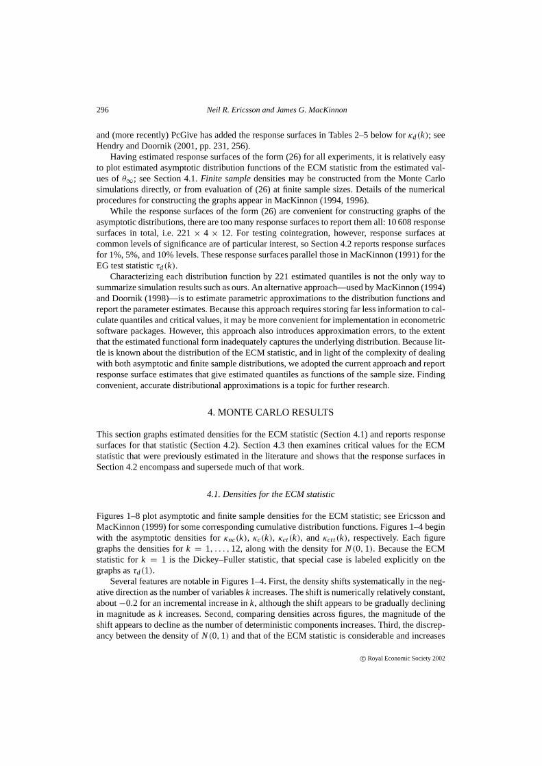
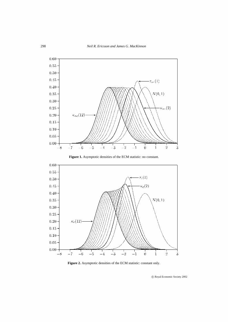
Figures 1–8 plot asymptotic and finite sample densities for the ECM statistic; see Ericsson andMacKinnon (1999) for some corresponding cumulative distribution functions. Figures 1–4 beginwith the asymptotic densities forκnc(k), κc(k), κct(k), andκctt(k), respectively. Each figuregraphs the densities fork = 1, . . . , 12, along with the density forN(0, 1). Because the ECMstatistic fork = 1 is the Dickey–Fuller statistic, that special case is labeled explicitly on thegraphs asτd(1).

Several features are notable in Figures 1–4. First, the density shifts systematically in the neg-ative direction as the number of variablesk increases. The shift is numerically relatively constant,about−0.2 for an incremental increase ink, although the shift appears to be gradually decliningin magnitude ask increases. Second, comparing densities across figures, the magnitude of theshift appears to decline as the number of deterministic components increases. Third, the discrep-ancy between the density ofN(0, 1) and that of the ECM statistic is considerable and increases



as the number of deterministic components and stochastic variables increases. Thus, inferencesabout cointegration when using the ECM statistic would be hazardous if (e.g.) a standardizednormal distribution were assumed. Fourth, the figures highlight the unique shape of the distribu-tion of the Dickey–Fuller statistic. Figure 1 in particular brings out the asymmetry in the densityof the Dickey–Fuller statisticτnc(1), a feature apparent in MacKinnon (1994, Figure 3) and alsonoted by Abadir (1995), both analytically and in his Figure 1.

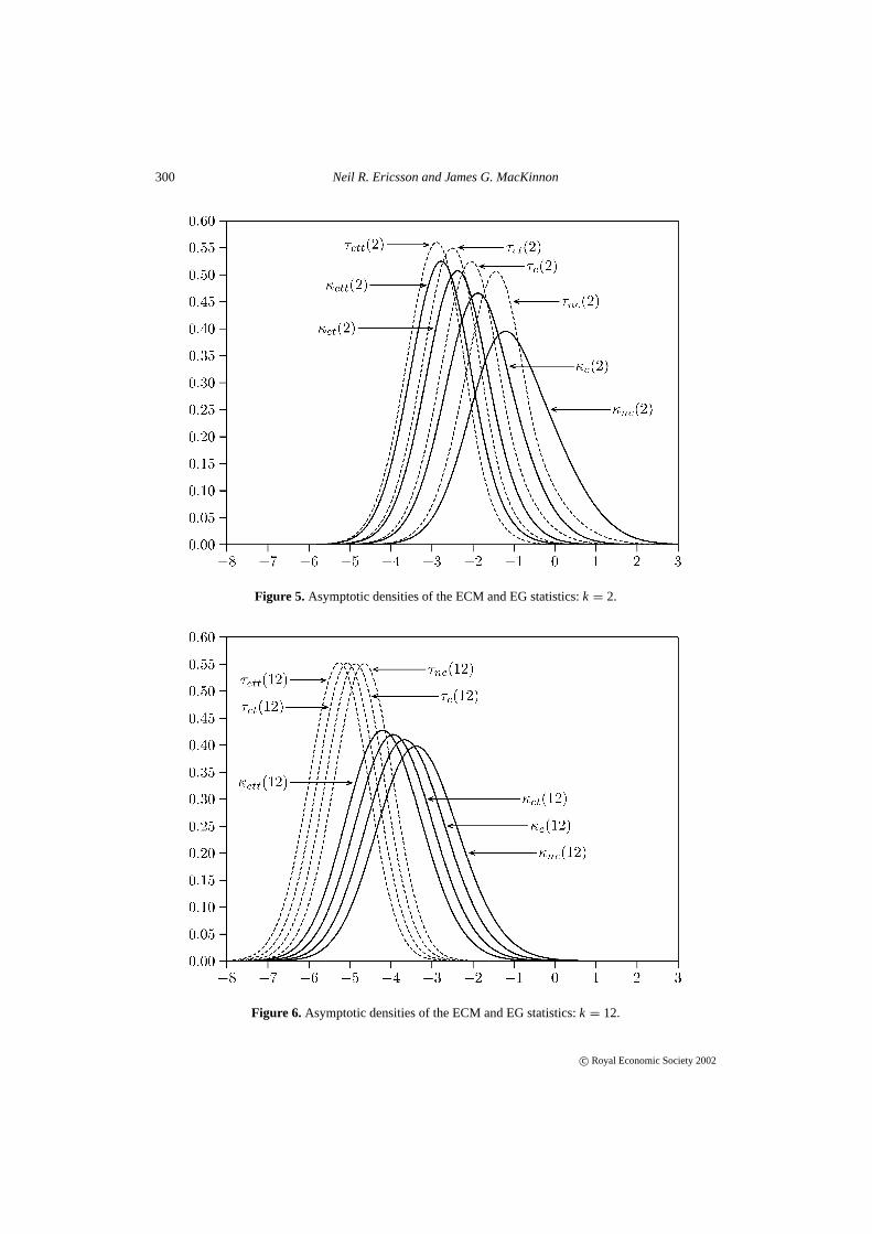
As discussed in Section 2, comparisons of the ECM and EG procedures are of considerableinterest. MacKinnon (1994, 1996) numerically estimated the distributions for the Dickey–Fullerstatistic applied to the EG cointegration residuals. Figures 5–6 plot the asymptotic densities ofthe ECM and EG statistics fork = 2 andk = 12, where the densities of the EG statisticτd(k)

are derived from MacKinnon’s (1996) simulations. For all choices of deterministic components,the density ofτd(k) is shifted to the left of that forκd(k), substantially so for larger values ofk.The density ofτd(2) is shifted by only a few tenths relative toκd(2), whereas that forτd(12) isoften shifted by one to two units relative toκd(12).

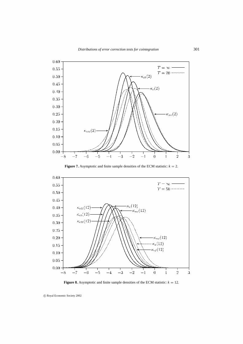
Figures 1–6 all concern asymptotic properties. While asymptotic properties are essential forunderstanding the nature of the ECM statistic, empirical sample sizes are often small, so it isvaluable to assess the discrepancies between asymptotic and finite sample distributions. Figures 7and 8 plot asymptotic and finite sample densities forκd(2) andκd(12), where ‘finite sample’ isT = 20 for κd(2) and T = 50 for κd(12). For all choices of deterministic components, theasymptotic densities tend to be more peaked than the finite sample ones, perhaps reflecting thecontribution of estimation uncertainty to the latter. While the finite sample densities tend to shiftto the left as the sample size increases, this does not hold uniformly for all parts of the density.Shifts to the right are notable in the left tails in Figure 7. Figures 7 and 8 each include thedensities for all four possibilities of deterministic components for a given ECM statistic. Eachadditional deterministic component systematically shifts the statistic’s density to the left, and theincremental shift is almost invariant to the total number of deterministic components.

4.2. Response surfaces for critical values

As just discussed, the distribution of the ECM statisticκd(k) depends systematically on the num-ber of variablesk, the number of deterministic componentsd, and the sample sizeT . The currentsubsection quantifies these dependencies through response surfaces for three quantiles: those at1%, 5%, and 10%.

To motivate these dependencies, consider Figure 9, which plots the data to be analyzed in theresponse surfaces. Specifically, each 3D graph in Figure 9 plots the within-experiment averagefor the estimated quantile againstk and(Ta/100)−1 (a rescaled inverse of the adjusted samplesize), given the choice ofd and the quantile’s percent levelp. The previously noted dependencieson d, k, T , and p are all apparent in Figure 9. Additionally,T appears to have relatively littleeffect on the 5% and 10% quantiles.

Tables 2–5 list the least squares estimates of the response surface coefficientsθ∞, θ1, θ2,andθ3 for the 1%, 5%, and 10% quantiles withk = 1, . . . , 12.5 The conditional ECM is esti-mated with no deterministic terms (Table 2), with a constant term only (Table 3), with a constantterm and a linear trend only (Table 4), and with a constant term, a linear trend, and a quadratic

5The response surfaces reported in Tables 2–5 differ slightly from those underlying Figures 1–8. The former are esti-mated by OLS, whereas the latter are estimated by GMM, using methods discussed in MacKinnon (1996). The twoapproaches yield numerically very similar results.



Figure 1. Asymptotic densities of the ECM statistic: no constant.

Figure 2. Asymptotic densities of the ECM statistic: constant only.



Figure 3. Asymptotic densities of the ECM statistic: constant and trend.

Figure 4. Asymptotic densities of the ECM statistic: constant, trend, and trend squared.



Figure 5. Asymptotic densities of the ECM and EG statistics:k = 2.

Figure 6. Asymptotic densities of the ECM and EG statistics:k = 12.



Figure 7. Asymptotic and finite sample densities of the ECM statistic:k = 2.

Figure 8. Asymptotic and finite sample densities of the ECM statistic:k = 12.



Figure 9. Estimated finite sample 1%, 5%, and 10% quantilesq(T) for the ECM statistic as a function ofd, k, andTa.

trend (Table 5). The tables also include the estimated standard error (‘s.e.’) forθ∞ to providea measure of uncertainty for the estimated asymptotic quantile. This standard error is alwayssmaller than 0.001, assuring high precision in the estimates. The estimated standard errors arejackknife heteroskedasticity consistent standard errors from MacKinnon and White (1985), asthe experimental design may induce some heteroskedasticity in the estimated quantiles acrossdifferent sample sizes.



Table 2. Response surface estimates for critical values of the ECM test of cointegrationκnc(k): no deter-ministic terms.

k Size (%) θ∞ (s.e.) θ1 θ2 θ3 σ

1 1 −2.5659 (0.0006) −2.19 −3.6 26 0.00843

5 −1.9408 (0.0003) −0.35 0.6 −17 0.00430

10 −1.6167 (0.0003) 0.23 −1.0 −6 0.00339

2 1 −3.2106 (0.0006) −4.69 −10.5 48 0.00845

5 −2.5937 (0.0003) −1.53 −0.8 −24 0.00439

10 −2.2643 (0.0003) −0.41 −1.5 −9 0.00350

3 1 −3.6215 (0.0006) −6.14 −5.3 −67 0.00892

5 −3.0048 (0.0003) −2.11 2.1 −61 0.00468

10 −2.6744 (0.0003) −0.57 1.2 −44 0.00372

4 1 −3.9433 (0.0006) −7.15 −3.1 −69 0.00929

5 −3.3268 (0.0003) −2.04 −6.4 19 0.00455

10 −2.9942 (0.0003) −0.21 −5.1 13 0.00377

5 1 −4.2168 (0.0005) −7.66 −2.1 −87 0.00920

5 −3.5978 (0.0003) −1.92 −3.6 −17 0.00502

10 −3.2637 (0.0003) 0.25 −4.2 −15 0.00405

6 1 −4.4585 (0.0006) −7.72 −7.2 −57 0.01034

5 −3.8373 (0.0003) −1.38 −7.7 −6 0.00519

10 −3.5022 (0.0002) 1.15 −11.1 12 0.00397

7 1 −4.6763 (0.0005) −7.78 −5.1 −73 0.01122

5 −4.0535 (0.0003) −0.76 −10.0 −7 0.00567

10 −3.7165 (0.0002) 2.04 −14.7 15 0.00421

8 1 −4.8772 (0.0006) −7.64 −2.4 −116 0.01035

5 −4.2513 (0.0003) −0.03 −12.0 −19 0.00543

10 −3.9135 (0.0002) 3.10 −20.3 25 0.00420

9 1 −5.0634 (0.0006) −7.13 −6.9 −113 0.01009

5 −4.4363 (0.0003) 1.00 −18.4 −8 0.00534

10 −4.0974 (0.0003) 4.46 −32.1 74 0.00422

10 1 −5.2381 (0.0006) −6.68 −4.7 −149 0.01035

5 −4.6093 (0.0003) 2.11 −25.4 10 0.00552

10 −4.2693 (0.0003) 5.76 −38.2 72 0.00419

11 1 −5.4039 (0.0006) −6.05 −7.1 −163 0.01038

5 −4.7734 (0.0004) 3.37 −35.4 48 0.00556

10 −4.4324 (0.0003) 7.33 −53.3 145 0.00426

12 1 −5.5598 (0.0006) −5.10 −19.4 −75 0.01040

5 −4.9279 (0.0004) 4.77 −48.8 109 0.00579

10 −4.5864 (0.0003) 8.96 −68.0 204 0.00439



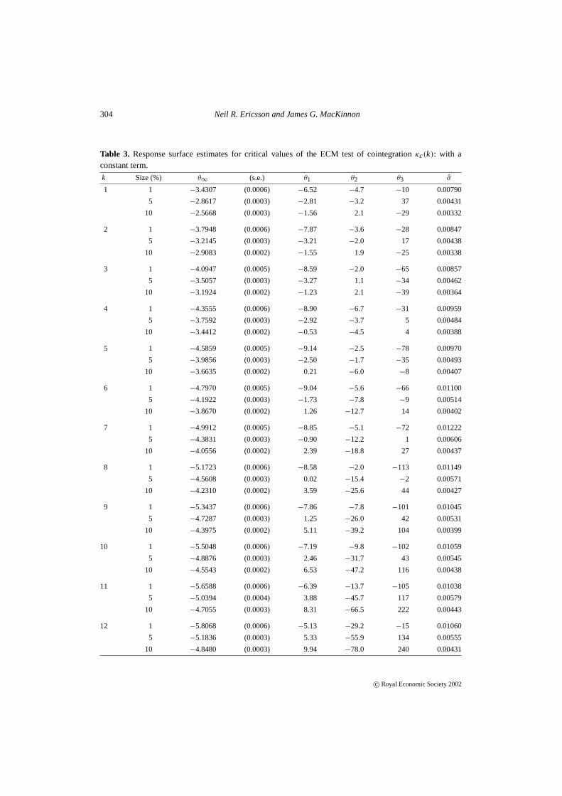
Table 3. Response surface estimates for critical values of the ECM test of cointegrationκc(k): with aconstant term.

k Size (%) θ∞ (s.e.) θ1 θ2 θ3 σ

1 1 −3.4307 (0.0006) −6.52 −4.7 −10 0.00790

5 −2.8617 (0.0003) −2.81 −3.2 37 0.00431

10 −2.5668 (0.0003) −1.56 2.1 −29 0.00332

2 1 −3.7948 (0.0006) −7.87 −3.6 −28 0.00847

5 −3.2145 (0.0003) −3.21 −2.0 17 0.00438

10 −2.9083 (0.0002) −1.55 1.9 −25 0.00338

3 1 −4.0947 (0.0005) −8.59 −2.0 −65 0.00857

5 −3.5057 (0.0003) −3.27 1.1 −34 0.00462

10 −3.1924 (0.0002) −1.23 2.1 −39 0.00364

4 1 −4.3555 (0.0006) −8.90 −6.7 −31 0.00959

5 −3.7592 (0.0003) −2.92 −3.7 5 0.00484

10 −3.4412 (0.0002) −0.53 −4.5 4 0.00388

5 1 −4.5859 (0.0005) −9.14 −2.5 −78 0.00970

5 −3.9856 (0.0003) −2.50 −1.7 −35 0.00493

10 −3.6635 (0.0002) 0.21 −6.0 −8 0.00407

6 1 −4.7970 (0.0005) −9.04 −5.6 −66 0.01100

5 −4.1922 (0.0003) −1.73 −7.8 −9 0.00514

10 −3.8670 (0.0002) 1.26 −12.7 14 0.00402

7 1 −4.9912 (0.0005) −8.85 −5.1 −72 0.01222

5 −4.3831 (0.0003) −0.90 −12.2 1 0.00606

10 −4.0556 (0.0002) 2.39 −18.8 27 0.00437

8 1 −5.1723 (0.0006) −8.58 −2.0 −113 0.01149

5 −4.5608 (0.0003) 0.02 −15.4 −2 0.00571

10 −4.2310 (0.0002) 3.59 −25.6 44 0.00427

9 1 −5.3437 (0.0006) −7.86 −7.8 −101 0.01045

5 −4.7287 (0.0003) 1.25 −26.0 42 0.00531

10 −4.3975 (0.0002) 5.11 −39.2 104 0.00399

10 1 −5.5048 (0.0006) −7.19 −9.8 −102 0.01059

5 −4.8876 (0.0003) 2.46 −31.7 43 0.00545

10 −4.5543 (0.0002) 6.53 −47.2 116 0.00438

11 1 −5.6588 (0.0006) −6.39 −13.7 −105 0.01038

5 −5.0394 (0.0004) 3.88 −45.7 117 0.00579

10 −4.7055 (0.0003) 8.31 −66.5 222 0.00443

12 1 −5.8068 (0.0006) −5.13 −29.2 −15 0.01060

5 −5.1836 (0.0003) 5.33 −55.9 134 0.00555

10 −4.8480 (0.0003) 9.94 −78.0 240 0.00431



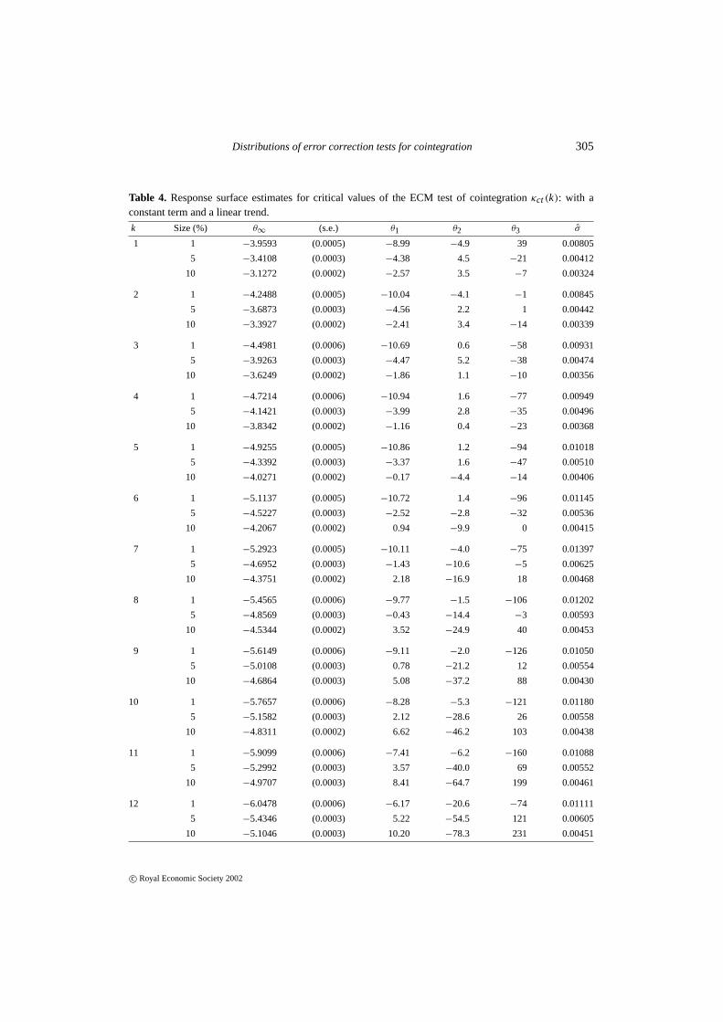
Table 4. Response surface estimates for critical values of the ECM test of cointegrationκct(k): with aconstant term and a linear trend.

k Size (%) θ∞ (s.e.) θ1 θ2 θ3 σ

1 1 −3.9593 (0.0005) −8.99 −4.9 39 0.00805

5 −3.4108 (0.0003) −4.38 4.5 −21 0.00412

10 −3.1272 (0.0002) −2.57 3.5 −7 0.00324

2 1 −4.2488 (0.0005) −10.04 −4.1 −1 0.00845

5 −3.6873 (0.0003) −4.56 2.2 1 0.00442

10 −3.3927 (0.0002) −2.41 3.4 −14 0.00339

3 1 −4.4981 (0.0006) −10.69 0.6 −58 0.00931

5 −3.9263 (0.0003) −4.47 5.2 −38 0.00474

10 −3.6249 (0.0002) −1.86 1.1 −10 0.00356

4 1 −4.7214 (0.0006) −10.94 1.6 −77 0.00949

5 −4.1421 (0.0003) −3.99 2.8 −35 0.00496

10 −3.8342 (0.0002) −1.16 0.4 −23 0.00368

5 1 −4.9255 (0.0005) −10.86 1.2 −94 0.01018

5 −4.3392 (0.0003) −3.37 1.6 −47 0.00510

10 −4.0271 (0.0002) −0.17 −4.4 −14 0.00406

6 1 −5.1137 (0.0005) −10.72 1.4 −96 0.01145

5 −4.5227 (0.0003) −2.52 −2.8 −32 0.00536

10 −4.2067 (0.0002) 0.94 −9.9 0 0.00415

7 1 −5.2923 (0.0005) −10.11 −4.0 −75 0.01397

5 −4.6952 (0.0003) −1.43 −10.6 −5 0.00625

10 −4.3751 (0.0002) 2.18 −16.9 18 0.00468

8 1 −5.4565 (0.0006) −9.77 −1.5 −106 0.01202

5 −4.8569 (0.0003) −0.43 −14.4 −3 0.00593

10 −4.5344 (0.0002) 3.52 −24.9 40 0.00453

9 1 −5.6149 (0.0006) −9.11 −2.0 −126 0.01050

5 −5.0108 (0.0003) 0.78 −21.2 12 0.00554

10 −4.6864 (0.0003) 5.08 −37.2 88 0.00430

10 1 −5.7657 (0.0006) −8.28 −5.3 −121 0.01180

5 −5.1582 (0.0003) 2.12 −28.6 26 0.00558

10 −4.8311 (0.0002) 6.62 −46.2 103 0.00438

11 1 −5.9099 (0.0006) −7.41 −6.2 −160 0.01088

5 −5.2992 (0.0003) 3.57 −40.0 69 0.00552

10 −4.9707 (0.0003) 8.41 −64.7 199 0.00461

12 1 −6.0478 (0.0006) −6.17 −20.6 −74 0.01111

5 −5.4346 (0.0003) 5.22 −54.5 121 0.00605

10 −5.1046 (0.0003) 10.20 −78.3 231 0.00451



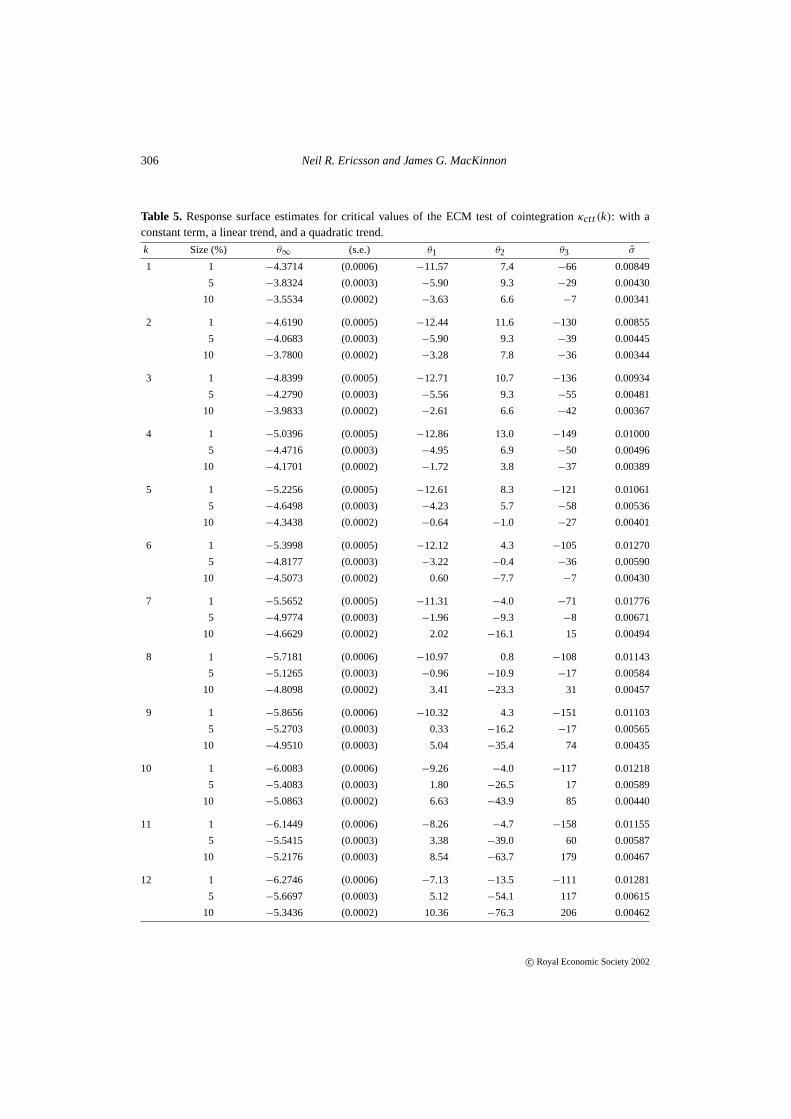
Table 5. Response surface estimates for critical values of the ECM test of cointegrationκctt(k): with aconstant term, a linear trend, and a quadratic trend.

k Size (%) θ∞ (s.e.) θ1 θ2 θ3 σ

1 1 −4.3714 (0.0006) −11.57 7.4 −66 0.00849

5 −3.8324 (0.0003) −5.90 9.3 −29 0.00430

10 −3.5534 (0.0002) −3.63 6.6 −7 0.00341

2 1 −4.6190 (0.0005) −12.44 11.6 −130 0.00855

5 −4.0683 (0.0003) −5.90 9.3 −39 0.00445

10 −3.7800 (0.0002) −3.28 7.8 −36 0.00344

3 1 −4.8399 (0.0005) −12.71 10.7 −136 0.00934

5 −4.2790 (0.0003) −5.56 9.3 −55 0.00481

10 −3.9833 (0.0002) −2.61 6.6 −42 0.00367

4 1 −5.0396 (0.0005) −12.86 13.0 −149 0.01000

5 −4.4716 (0.0003) −4.95 6.9 −50 0.00496

10 −4.1701 (0.0002) −1.72 3.8 −37 0.00389

5 1 −5.2256 (0.0005) −12.61 8.3 −121 0.01061

5 −4.6498 (0.0003) −4.23 5.7 −58 0.00536

10 −4.3438 (0.0002) −0.64 −1.0 −27 0.00401

6 1 −5.3998 (0.0005) −12.12 4.3 −105 0.01270

5 −4.8177 (0.0003) −3.22 −0.4 −36 0.00590

10 −4.5073 (0.0002) 0.60 −7.7 −7 0.00430

7 1 −5.5652 (0.0005) −11.31 −4.0 −71 0.01776

5 −4.9774 (0.0003) −1.96 −9.3 −8 0.00671

10 −4.6629 (0.0002) 2.02 −16.1 15 0.00494

8 1 −5.7181 (0.0006) −10.97 0.8 −108 0.01143

5 −5.1265 (0.0003) −0.96 −10.9 −17 0.00584

10 −4.8098 (0.0002) 3.41 −23.3 31 0.00457

9 1 −5.8656 (0.0006) −10.32 4.3 −151 0.01103

5 −5.2703 (0.0003) 0.33 −16.2 −17 0.00565

10 −4.9510 (0.0003) 5.04 −35.4 74 0.00435

10 1 −6.0083 (0.0006) −9.26 −4.0 −117 0.01218

5 −5.4083 (0.0003) 1.80 −26.5 17 0.00589

10 −5.0863 (0.0002) 6.63 −43.9 85 0.00440

11 1 −6.1449 (0.0006) −8.26 −4.7 −158 0.01155

5 −5.5415 (0.0003) 3.38 −39.0 60 0.00587

10 −5.2176 (0.0003) 8.54 −63.7 179 0.00467

12 1 −6.2746 (0.0006) −7.13 −13.5 −111 0.01281

5 −5.6697 (0.0003) 5.12 −54.1 117 0.00615

10 −5.3436 (0.0002) 10.36 −76.3 206 0.00462



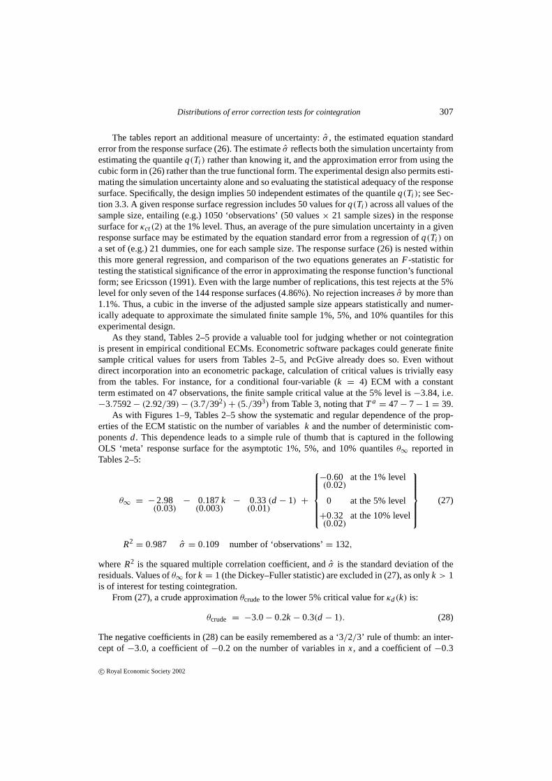
The tables report an additional measure of uncertainty:σ , the estimated equation standarderror from the response surface (26). The estimateσ reflects both the simulation uncertainty fromestimating the quantileq(Ti ) rather than knowing it, and the approximation error from using thecubic form in (26) rather than the true functional form. The experimental design also permits esti-mating the simulation uncertainty alone and so evaluating the statistical adequacy of the responsesurface. Specifically, the design implies 50 independent estimates of the quantileq(Ti ); see Sec-tion 3.3. A given response surface regression includes 50 values forq(Ti ) across all values of thesample size, entailing (e.g.) 1050 ‘observations’ (50 values× 21 sample sizes) in the responsesurface forκct(2) at the 1% level. Thus, an average of the pure simulation uncertainty in a givenresponse surface may be estimated by the equation standard error from a regression ofq(Ti ) ona set of (e.g.) 21 dummies, one for each sample size. The response surface (26) is nested withinthis more general regression, and comparison of the two equations generates anF-statistic fortesting the statistical significance of the error in approximating the response function’s functionalform; see Ericsson (1991). Even with the large number of replications, this test rejects at the 5%level for only seven of the 144 response surfaces (4.86%). No rejection increasesσ by more than1.1%. Thus, a cubic in the inverse of the adjusted sample size appears statistically and numer-ically adequate to approximate the simulated finite sample 1%, 5%, and 10% quantiles for thisexperimental design.

As they stand, Tables 2–5 provide a valuable tool for judging whether or not cointegrationis present in empirical conditional ECMs. Econometric software packages could generate finitesample critical values for users from Tables 2–5, and PcGive already does so. Even withoutdirect incorporation into an econometric package, calculation of critical values is trivially easyfrom the tables. For instance, for a conditional four-variable (k = 4) ECM with a constantterm estimated on 47 observations, the finite sample critical value at the 5% level is−3.84, i.e.−3.7592− (2.92/39) − (3.7/392) + (5./393) from Table 3, noting thatTa

= 47− 7− 1 = 39.As with Figures 1–9, Tables 2–5 show the systematic and regular dependence of the prop-

erties of the ECM statistic on the number of variablesk and the number of deterministic com-ponentsd. This dependence leads to a simple rule of thumb that is captured in the followingOLS ‘meta’ response surface for the asymptotic 1%, 5%, and 10% quantilesθ∞ reported inTables 2–5:

θ∞ = −2.98(0.03)

− 0.187(0.003)

k − 0.33(0.01)

(d − 1) +

−0.60(0.02)

at the 1% level

0 at the 5% level

+0.32(0.02)

at the 10% level

(27)

R2= 0.987 σ = 0.109 number of ‘observations’= 132,

whereR2 is the squared multiple correlation coefficient, andσ is the standard deviation of theresiduals. Values ofθ∞ for k = 1 (the Dickey–Fuller statistic) are excluded in (27), as onlyk > 1is of interest for testing cointegration.

From (27), a crude approximationθcrude to the lower 5% critical value forκd(k) is:

θcrude = −3.0 − 0.2k − 0.3(d − 1). (28)

The negative coefficients in (28) can be easily remembered as a ‘3/2/3’ rule of thumb: an inter-cept of−3.0, a coefficient of−0.2 on the number of variables inx, and a coefficient of−0.3



Figure 10. Estimated asymptotic 1%, 5%, and 10% quantilesθ∞ for the ECM statistic as a function ofkandd.

on the number of deterministic terms over and above a constant term. For the ECM evaluatedearlier (k = 4, d = 1, T = 47), θcrude is −3.8, deviating by only 0.04 from the value of−3.84calculated with Table 3. While deviations betweenθcrudeandq(Ti ) may be larger or smaller thanthis for otherk, d, andT , it is well worth keeping in mind that, with typical macroeconomic data,the ECM statistic itself can easily fluctuate by a few tenths, simply by adding or dropping a fewobservations from the sample.

Figure 10 highlights this near-linear dependence of the asymptotic quantileθ∞ on k andd.Each 3D graph in Figure 10 plotsθ∞ againstk andd, given the quantile’s percent levelp. Thesurfaces are virtually planar except for the Dickey–Fuller statistic (k = 1), which is excludedfrom (27) and (28).

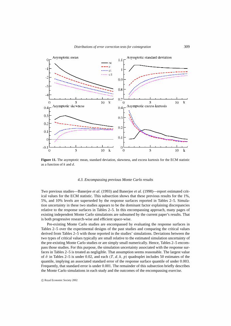
The asymptotic moments of the ECM statistic also show marked regularity in the distribu-tion’s behavior. Figure 11 plots its asymptotic mean, standard deviation, skewness, and excesskurtosis as a function ofk andd.6 The asymptotic mean declines by approximately 0.2 and 0.4respectively for unit increases ink and d, close to the estimated shifts for the critical valuesin (27). While the asymptotic standard deviation, skewness, and excess kurtosis also depend onk andd, those dependencies are numerically much smaller than that of the asymptotic mean.For all values ofk andd examined, the asymptotic standard deviation is close to unity, and theasymptotic skewness and excess kurtosis are close to zero. These results reconfirm the visualcharacterization from Figures 1–8: the distribution of the ECM statisticκd(k) is relatively closeto normality with unit variance. In light of these observations, parametric distributional approx-imations to the distribution of the ECM statistic may be promising—perhaps using the normaldistribution, Student’st-distribution, or an expansion thereon.

Equations (27) and (28) quantify the straightforward dependencies of the ECM statistic’squantiles onk andd, they provide a mechanism for extrapolating critical values for values ofkandd outside the experimental design (25), and they offer a rough-and-ready way of assessingempirical results when Tables 2–5 are not available. Preferably, though, Tables 2–5 or the relatedcomputer program should be used.

6The asymptotic moments were calculated by response surfaces from a separate set of Monte Carlo experiments,following an approach like that used for the quantiles. Monte Carlo estimation of the statistic’s finite sample momentsdoes assume the existence of those moments. However, even if those moments are infinite, their Monte Carlo estimatesmay be close to the (finite) moments of a Nagar approximation to the statistic; see Sargan (1982).



Figure 11. The asymptotic mean, standard deviation, skewness, and excess kurtosis for the ECM statisticas a function ofk andd.

4.3. Encompassing previous Monte Carlo results

Two previous studies—Banerjeeet al. (1993) and Banerjeeet al. (1998)—report estimated crit-ical values for the ECM statistic. This subsection shows that these previous results for the 1%,5%, and 10% levels are superseded by the response surfaces reported in Tables 2–5. Simula-tion uncertainty in these two studies appears to be the dominant factor explaining discrepanciesrelative to the response surfaces in Tables 2–5. In this encompassing approach, many pages ofexisting independent Monte Carlo simulations are subsumed by the current paper’s results. Thatis both progressive research-wise and efficient space-wise.

Pre-existing Monte Carlo studies are encompassed by evaluating the response surfaces inTables 2–5 over the experimental designs of the past studies and comparing the critical valuesderived from Tables 2–5 with those reported in the studies’ simulations. Deviations between thetwo types of critical values typically are small relative to the estimated simulation uncertainty ofthe pre-existing Monte Carlo studies or are simply small numerically. Hence, Tables 2–5 encom-pass those studies. For this purpose, the simulation uncertainty associated with the response sur-faces in Tables 2–5 is treated as negligible. That assumption seems reasonable. The largest valueof σ in Tables 2–5 is under 0.02, and each(T, d, k, p) quadruplet includes 50 estimates of thequantile, implying an associated standard error of the response surface quantile of under 0.003.Frequently, that standard error is under 0.001. The remainder of this subsection briefly describesthe Monte Carlo simulations in each study and the outcomes of the encompassing exercise.



Banerjeeet al. (1993, Table 7.6, p. 233) report estimated critical values at the 1%, 5%, and10% levels forκc(2) at T = (25, 50, 100), using 5000 replications per experiment. Deviationsrelative to the response surfaces from Table 3 are all under 0.1 in absolute value. Using thevalues ofσ in Table 3 as a benchmark and rescaling by the square root of the ratio of simula-tions calculated, the estimated standard errors for the three quantiles in Banerjeeet al. (1993)are approximately 0.063, 0.032, and 0.025. The observed discrepancies between the estimatedquantiles in Banerjeeet al. (1993) and those calculated from Table 3 appear as expected, giventhe simulation uncertainty of the former.

Banerjeeet al. (1998, Table I) report estimated critical values at the 1%, 5%, 10%, and25% levels forκc(k) and κct(k) (k = 2, . . . , 6) at T = (25, 50, 100, 500, ∞), using 25 000replications per experiment. Deviations relative to the response surfaces from Tables 3 and 4 areall under 0.2 in absolute value, and are typically 0.04 or smaller in magnitude. The estimatedstandard errors for the 1%, 5%, and 10% quantiles in Banerjeeet al. (1998) are approximately0.028, 0.014, and 0.011.

5. TWO EMPIRICAL APPLICATIONS

This section applies the finite sample critical values derived earlier and the computer program forcalculatingp-values to two empirical ECMs. Section 5.1 considers a model of UK narrow moneydemand from Hendry and Ericsson (1991), and Section 5.2 a model of US federal governmentdebt from Hamilton and Flavin (1986). (Ericsson and MacKinnon (1999) also assess the modelof UK consumers’ expenditure from Davidsonet al.(1978).) The model in Hendry and Ericsson(1991) has played a significant role in the literature on ECMs and cointegration, and Hamiltonand Flavin (1986) was one of the early papers to employ unit root statistics for testing economichypotheses. Each subsection briefly reviews the estimated equation and considers correspondingconditional ECM tests. Tables summarize the results, reporting the empiricalt-values for testingcointegration, along with critical values andp-values. Use of the critical values from Tables 2–5for the ECM statistic affects the economic inferences drawn.

Several issues arise in testing for cointegration in these models. First, the ECM for moneydemand was derived from an unrestricted ADL. Both the ADL and the ECM allow testing ofcointegration, although the ECM requires slight modification to apply the critical values fromTables 2–5. Second, dynamic specification affects the degrees of freedom used in estimation.Hence, when computing critical values, the adjusted sample sizeTa is calculated asT −h (ratherthan asT − (2k + d − 1)), whereh is the total number of regressors, including deterministicvariables. The calculation ofp-values utilizesh similarly. Third, the choice of deterministicvariables affects thet-values and the corresponding critical values andp-values, so potentiallyaffecting inference. Finally, nonlinearity of the deterministic trend and lack of weak exogeneityare important in the model of government debt. Throughout this section, capital letters denoteboth the generic name and the level of a variable, logarithms are in lowercase, and OLS standarderrors are in parentheses.

5.1. UK narrow money demand

Hendry and Ericsson (1991, equation (6)) model UK narrow money demand as a conditional



ECM, whose final parsimonious form is as follows:

1(m − p)t = − 0.687(0.125)

1pt − 0.175(0.058)

1(m − p − i )t−1 − 0.630(0.060)

Rnett

− 0.0929(0.0085)

(m − p − i )t−1 + 0.0234(0.0040)

(29)

T = 100 (1964Q3–1989Q2) R2= 0.76 σ = 1.313%.

The data are nominal narrow moneyM1 (M , in £ millions), real total final expenditure (TFE)at 1985 prices (I , in £ millions), the TFE deflator (P, 1985 = 1.00), and the net interest rate(Rnet, in percent per annum expressed as a fraction). The last series is the difference between thethree-month local authority interest rate and a learning-adjusted retail sight-deposit interest rate.

While thet-value on the error correction term(m− p−i )t−1 in (29) is very large and negative(−10.87), significance levels are not known, given the presence of nuisance parameters; see Kre-merset al.(1992) and Kiviet and Phillips (1992). This difficulty arises because one of the coeffi-cients in the cointegrating vector—the long-run income elasticity—is constrained. One solutionis to estimate that coefficient unrestrictedly, as occurs when estimating (29) withi t−1 added:

1(m − p)t = − 0.702(0.128)

1pt − 0.178(0.058)

1(m − p − i )t−1 − 0.611(0.067)

Rnett

− 0.0882(0.0113)

(m − p − i )t−1 + 0.0065(0.0104)

i t−1 − 0.049(0.117)

(30)

T = 100 (1964Q3–1989Q2) R2= 0.76 σ = 1.317%.

The t-value on(m − p − i )t−1 in (30) is−7.78, which is significant at the 1% level forκc(4),with critical value of−4.45. In fact, the finite samplep-value for−7.78 is 0.0000.

Equations (29) and (30) can be derived from an unrestricted fifth-order ADL model inm− p,1p, i , and Rnet. The ECM statistic for that ADL is−5.17, also significant at the 1% level forκc(4), with critical value of−4.47. Its finite samplep-value is 0.0014, suggesting a minor lossin power from estimating additional coefficients on dynamics relative to (30).

Both this fifth-order ADL and the ECM in (30) include one deterministic component: a con-stant term. Table 6 reports the statisticκd(4) for the four choices of deterministic componentsconsidered in the sections earlier; the value ofh; the finite sample, asymptotic, and crude criticalvalues at the 1%, 5%, and 10% levels; finite sample and asymptoticp-values; the estimated equa-tion standard errorσ ; and anF-statistic for testing the significance of omitted deterministic com-ponents. The symbols+, ∗, and∗∗ denote rejection at the 10%, 5%, and 1% levels, respectively.With a constant term, linear trend, and quadratic trend included, the statisticκctt(4) is insignif-icant at the 10% level for both the ADL and the ECM: theirp-values are 0.3859 and 0.4544.With fewer deterministic components, cointegration is detected at the 0.5% level or smaller inthe ADL and the ECM, as the statisticsκct(4), κc(4), andκnc(4) show.

The final column in Table 6 lists theF-statistics for testing the significance of the omitteddeterministic components in the corresponding regressions, relative to the regressions for obtain-ing κctt(4): degrees of freedom for theF-statistics appear in parentheses asF( · , · ), and thestatistics’ p-values are in brackets[ · ]. TheseF-statistics indicate that the constant term, lin-ear trend, and quadratic trend are statistically insignificant, so all the reported ECM statisticsin Table 6 make statistically justifiable assumptions about these deterministic components. The



Table 6. Empirical t-values, critical values, andp-values for the ECM statistic: models of UK narrowmoney demand.

Statistic Empirical h Critical value p-value σ F-statisticModel or t-value 1% 5% 10% Finite Asymp- (%) vs. the modelcalculation sample totic forκctt(4)

κctt(4)

ADL −3.29 26 −5.21 −4.54 −4.19 0.3859 0.4140 1.313 —

ECM −3.14 8 −5.18 −4.52 −4.19 0.4544 0.4819 1.326 —

Asymptotic — — −5.04 −4.47 −4.17 — — — —

Crude — — −5.0 −4.4 −4.1 — — — —

κct(4)

ADL −5.14∗∗ 25 −4.87 −4.19 −3.85 0.0047 0.0024 1.306 F(1, 74) = 0.11 [0.74]

ECM −6.53∗∗ 7 −4.84 −4.18 −3.85 0.0000 0.0000 1.320 F(1, 92) = 0.16 [0.69]

Asymptotic — — −4.72 −4.14 −3.83 — — — —

Crude — — −4.7 −4.1 −3.8 — — — —

κc(4)

ADL −5.17∗∗ 24 −4.47 −3.80 −3.45 0.0014 0.0006 1.301 F(2, 74) = 0.28 [0.76]

ECM −7.78∗∗ 6 −4.45 −3.79 −3.45 0.0000 0.0000 1.317 F(2, 92) = 0.37 [0.69]

Asymptotic — — −4.36 −3.76 −3.44 — — — —

Crude — — −4.4 −3.8 −3.5 — — — —

κnc(4)

ADL −6.10∗∗ 23 −4.04 −3.35 −3.00 0.0000 0.0000 1.297 F(3, 74) = 0.36 [0.78]

ECM −10.57∗∗ 5 −4.02 −3.35 −3.00 0.0000 0.0000 1.311 F(3, 92) = 0.31 [0.82]

Asymptotic — — −3.94 −3.33 −2.99 — — — —

Crude — — −4.1 −3.5 −3.2 — — — —

statisticsκnc(4), κc(4), andκct(4) reject at standard levels, butκctt(4) does not, pointing to thevalue of parsimony in deterministic components for obtaining increased power of the cointegra-tion test, when parsimony is merited. The insignificance of a linear trend is particularly interest-ing. In a system analysis of this dataset, Hendry and Mizon (1993) find a second cointegratingvector, which includes a linear trend; but in their system model, that cointegrating vector doesnot enter the equation for money.

Table 6 lists the asymptotic and crude critical values at the 1%, 5%, and 10% levels, andthese differ by at most 0.21 from the calculated finite sample critical values. Likewise, the finitesample and asymptoticp-values in the table differ by only modest amounts. These numericallysmall discrepancies are not surprising because the sample size is relatively large (T = 100).

5.2. US federal government debt

The second model is an ADL from Hamilton and Flavin (1986, p. 816), relating real US federalgovernment debt to a deterministic nonlinear trend or ‘bubble’(1 + r )t and the budget surplus:



Bt = 48.41(26.40)

− 22.68(21.29)

(1 + r )t+ 0.69

(0.21)Bt−1 + 0.20

(0.24)Bt−2

− 1.30(0.13)

St − 0.63(0.31)

St−1 (31)

T = 23 (1962–1984) R2= 0.98 σ = 7.405.

The data are the adjusted debt (B) for the end of the fiscal year and the adjusted surplus (S)for the fiscal year (both in $ millions, 1967 prices). The variabler is set to 0.0112, the averageex postreal interest rate on US government bonds over 1960–84. The coefficient on(1 + r )t

is statistically insignificant, consistent with the absence of a speculative bubble. From this andrelated evidence, Hamilton and Flavin (1986, pp. 816–817) conclude that ‘. . . the data appearquite consistent with the assertion that the government has historically operated subject to theconstraint that expenditures not exceed receipts in expected present-value terms’.

This interpretation of the evidence assumes a long-run solution to (31) relating debt andsurplus. That is equivalent to assuming both cointegration betweenB and S, and the presenceof the corresponding cointegrating vector in (31). Empirically, however, (31) does not supportcointegration ofB andS. Rewriting (31) as an unrestricted ECM yields the following equation:

1Bt = 48.41(26.40)

− 22.68(21.29)

(1 + r )t− 0.104

(0.076)Bt−1 − 0.20

(0.24)1Bt−1

− 1.30(0.13)

1St − 1.92(0.36)

St−1 (32)

T = 23 (1962–1984) R2= 0.94 σ = 7.405.

The t-value onBt−1 is −1.36, which is insignificant at the 10% level forκct(2), with criticalvalue of−3.53. Using the critical value forκct(2) assumes that(1 + r )t is well approximatedby a linear trend, which, visually, it is. Alternatively, the 10% critical value forκctt(2) is −3.95,again with no rejection. The finite samplep-values under these two alternative assumptions are0.8386 and 0.9247. Notably, estimating (32) (or (31)) witht and t2 rather than with(1 + r )t

obtains a statistically significantly better fitting model, pointing to mis-specification in (32).Table 7 reports thet-values and critical values for (32) with various choices of deterministic

components. The bubble(1 + r )t is statistically insignificant in (32), whereas a linear trend andquadratic trend in its stead are statistically significant. Even so, the resultingt-value forκctt(2)

is −2.96, which is insignificant at the 10% level, having ap-value of 0.3689. Cointegration doesnot appear to hold in this conditional model, undercutting the economic inferences drawn byHamilton and Flavin (1986).

The sample size in (32) is small:T = 23. Correspondingly, the finite sample adjustmentsfor critical values are typically larger numerically in Table 7 than in Table 6, with the largestadjustment being−0.72 at the 1% level, i.e. about two thirds of a standard error in thet-value.The p-values have small finite sample adjustments, which mainly reflect each reportedt-valuebeing far from the lower tail of the associated density; cf. Figure 7.

The single-equation results in Table 7 all assume thatS is weakly exogenous, whereasSdoesnot appear to be so empirically. Starting with a second-order VAR inB andS, a single cointegrat-ing vector is apparent from the Johansen procedure when(1 + r )t or a linear trend is restrictedto lie in the cointegration space. Weak exogeneity ofS is rejected, as is that ofB, invalidatingcointegration analysis in a conditional single equation such as (31). Without weak exogeneity,



Table 7. Empirical t-values, critical values, andp-values for the ECM statistic: models of US federalgovernment debt.

Statistic Empirical h Critical value p-value σ F-statisticModel or t-value 1% 5% 10% Finite Asymp- vs. the modelcalculation sample totic forκctt(2)

κctt(2)

ADL + bubble −1.36 6 −5.34 −4.39 −3.95 0.9247 0.9651 7.40 —

ADL −2.96 7 −5.38 −4.41 −3.96 0.3689 0.4121 6.37 —

Asymptotic — — −4.62 −4.07 −3.78 — — — —

Crude — — −4.6 −4.0 −3.7 — — — —

κct(2)

ADL + bubble −1.36 6 −4.85 −3.95 −3.53 0.8386 0.8947 7.40 —

ADL −1.38 6 −4.85 −3.95 −3.53 0.8308 0.8886 7.38 F(1, 16) = 6.82 [0.02]

Asymptotic — — −4.25 −3.69 −3.39 — — — —

Crude — — −4.3 −3.7 −3.4 — — — —

κc(2)

ADL + bubble — — — — — — — — —

ADL −1.50 5 −4.25 −3.40 −2.99 0.5944 0.6458 7.43 F(2, 16) = 4.26 [0.03]

Asymptotic — — −3.79 −3.21 −2.91 — — — —

Crude — — −4.0 −3.4 −3.1 — — — —

κnc(2)

ADL + bubble — — — — — — — — —

ADL +2.58 4 −3.48 −2.68 −2.29 0.9984 0.9992 7.94 F(3, 16) = 4.52 [0.02]

Asymptotic — — −3.21 −2.59 −2.26 — — — —

Crude — — −3.7 −3.1 −2.8 — — — —

single equation inference about cointegration is hazardous at best; and testing the implied exo-geneity assumptions is clearly important. For example, in the Johansen procedure, the coefficienton the bubble(1 + r )t or on the linear trend is statistically significant and negatively relatedto B, whichever type of trend is included. That contrasts with the statistical insignificance of thecoefficient on(1+ r )t in (31). Furthermore, the negative coefficient on the trend is economicallysurprising and puzzling, although it may be indicative of certain non-ergodic features of the data:see Kremers (1988)inter alia.

In summary, the first empirical analysis illustrates the importance of parsimony, both in thechoice of deterministic terms and in the reduction from an ADL to a simpler ECM. The sec-ond analysis shows that mis-specification can render inference hazardous, even when the mis-specification is indirect, as with a violation of weak exogeneity. Imposition of valid restrictionson the cointegrating vector may increase power, although asymptotically correct critical valuesfor such ECM statistics have been derived only for the case when all cointegrating coefficientsare known; see Hansen (1995, Table 1).



6. CONCLUSIONS

This paper has assessed the distributional properties of the ECM statistic for testing cointegration.Graphs and response surfaces provide complementary summaries of the vast array of resultsfrom the Monte Carlo study undertaken. Both the graphs and the response surfaces highlightsome simple dependencies of the quantiles on the number of variables in the ECM, the choiceof deterministic components, and the estimation sample size. The reported response surfacesprovide a computationally convenient way for calculating finite sample critical values at the1%, 5%, and 10% levels. The response surfaces also encompass and supersede much of theliterature’s previous estimates of critical values for the ECM statistic. A computer program, freelyavailable over the Internet, can be used to calculatep-values and critical values at any level.Empirical conditional ECMs are ubiquitous in the cointegration literature, so these tools shouldbe of immediate use to the empirical modeler. Two previous empirical studies illustrate howcritical values andp-values for the ECM statistic can be employed in practice, and how their usemay affect economic inferences.

Several limitations of the current study come to mind, thereby suggesting some possibleextensions. First, the model’s lag order is assumed to be (and is) unity throughout the MonteCarlo analysis. For longer lags, the adjusted sample size may be corrected for additional degreesof freedom lost in estimation and thence used to calculate critical values from a response sur-face, as in Section 5. This refinement may not be sufficient in itself, so an extended analysis,such as in Cheung and Lai (1995) for the Dickey–Fuller statistic, may be required. Second, allof the ECM statistics with deterministic components have those components fully unconstrainedin estimation. In analyzing similar statistics, Harboet al. (1998) and Doorniket al. (1998) arguestrongly for constraining the highest-order deterministic component to lie in the cointegrationspace, so distributional properties for so constrained versions ofκc(k), κct(k), andκctt(k) areof interest. That said, virtually all empirically calculated ECM statistics to date have been withunconstrained deterministic components. Finally, the current paper has considered the proper-ties of the ECM statistic only under the null of no cointegration. While Banerjeeet al. (1993),Camposet al. (1996), and Banerjeeet al. (1998) present some calculations on the power of theECM statistic, further analysis could be illuminating, particularly comparisons with the Johansenprocedure and the EG procedure under various assumptions about weak exogeneity and commonfactor restrictions.

ACKNOWLEDGEMENTS

The views in this paper are solely the responsibility of the authors and should not be interpretedas reflecting the views of the Board of Governors of the Federal Reserve System or of any otherperson associated with the Federal Reserve System. JGM’s research was supported in part bygrants from the Social Sciences and Humanities Research Council of Canada. An early versionof this paper appeared under the title ‘Finite Sample Properties of Error Correction Tests forCointegration’, and an intermediate version was circulated as Ericsson and MacKinnon (1999).We are grateful to Shaghil Ahmed, David Bowman, Jon Faust, David Hendry, Søren Johansen,Fred Joutz, Andy Levin, Jaime Marquez, Bent Nielsen, John Rogers, Neil Shephard, an editor,and an anonymous referee for helpful comments and discussion; to Hayden Smith and SebastianThomas for research assistance; and to Jurgen Doornik and David Hendry for providing us witha beta-test version of GiveWin Version 2. Monte Carlo simulations and the graphs of the densi-ties were obtained from modified versions of programs for MacKinnon (1994, 1996). Response



surfaces were obtained using PcGive Professional Version 9.2, and 3D graphics were generatedfrom GiveWin Version 2.02: see Doornik and Hendry (2001). The paper’s tables of responsesurface coefficients and the Excel spreadsheet and Fortran program for calculating critical valuesand p-values are available from JGM’s home page.

REFERENCES

Abadir, K. M. (1995). The limiting distribution of thet ratio under a unit root.Econometric Theory 11,775–93.

Banerjee, A., J. J. Dolado, J. W. Galbraith and D. F. Hendry (1993).Co-integration, Error Correction, andthe Econometric Analysis of Non-stationary Data. Oxford: Oxford University Press.

Banerjee, A., J. J. Dolado and R. Mestre (1998). Error-correction mechanism tests for cointegration ina single-equation framework.Journal of Time Series Analysis 19, 267–83.

Banerjee, A. and D. F. Hendry (eds) (1996). The econometrics of economic policy, Special issue.OxfordBulletin of Economics and Statistics 58, 567–819.

Boswijk, H. P. (1994). Testing for an unstable root in conditional and structural error correction models.Journal of Econometrics 63, 37–60.

Boswijk, H. P. and P. H. Franses (1992). Dynamic specification and cointegration.Oxford Bulletin of Eco-nomics and Statistics 54, 369–81.

Campos, J., N. R. Ericsson and D. F. Hendry (1996). Cointegration tests in the presence of structural breaks.Journal of Econometrics 70, 187–220.

Cheung, Y.-W. and K. S. Lai (1995). Lag order and critical values of the augmented Dickey-Fuller test.Journal of Business and Economic Statistics 13, 277–80.

Davidson, J. E. H., D. F. Hendry, F. Srba and S. Yeo (1978). Econometric modelling of the aggregatetime-series relationship between consumers’ expenditure and income in the United Kingdom.EconomicJournal 88, 661–92.

Dickey, D. A. and W. A. Fuller (1981). Likelihood ratio statistics for autoregressive time series with a unitroot.Econometrica 49, 1057–72.

Doornik, J. A. (1998). Approximations to the asymptotic distributions of cointegration tests.Journal ofEconomic Surveys 12, 573–93. Erratum in (1999)13, i.

Doornik, J. A. and D. F. Hendry (2001).PcGive Version 10 for Windows. London: Timberlake ConsultantsPress.

Doornik, J. A., D. F. Hendry and B. Nielsen (1998). Inference in cointegrating models: UK M1 revisited.Journal of Economic Surveys 12, 533–72.

Elliott, G. (1995). Tests for the correct specification of cointegrating vectors and the error correction model.Mimeo. La Jolla, CA: Department of Economics, University of California at San Diego.

Engle, R. F. and C. W. J. Granger (1987). Co-integration and error correction: representation, estimation,and testing.Econometrica 55, 251–76.

Ericsson, N. R. (1991). Monte Carlo methodology and the finite sample properties of instrumental variablesstatistics for testing nested and non-nested hypotheses.Econometrica 59, 1249–77.

Ericsson, N. R. (ed.) (1998). Exogeneity, cointegration, and economic policy analysis. Special section,Journal of Business and Economic Statistics 16, 369–449.

Ericsson, N. R. and J. G. MacKinnon (1999). Distributions of error correction tests for cointegration. Inter-national finance discussion paper no. 655, Board of Governors of the Federal Reserve System, Wash-ington, D.C. December, available on the WorldWide Web atwww.federalreserve.gov/pubs/ifdp/

1999/655/default.htm.



Fuller, W. A. (1976).Introduction to Statistical Time Series. New York: John Wiley and Sons.Hamilton, J. D. and M. A. Flavin (1986). On the limitations of government borrowing: a framework for

empirical testing.American Economic Review 76, 808–19.Hammersley, J. M. and D. C. Handscomb (1964).Monte Carlo Methods. London: Chapman and Hall.Hansen, B. E. (1995). Rethinking the univariate approach to unit root testing: using covariates to increase

power.Econometric Theory 11, 1148–71.Harbo, I., S. Johansen, B. Nielsen and A. Rahbek (1998). Asymptotic inference on cointegrating rank in

partial systems.Journal of Business and Economic Statistics 16, 388–99.Hendry, D. F. (1984). Monte Carlo experimentation in econometrics. In Z. Griliches and M. D. Intriliga-

tor (eds),Handbook of Econometrics, Ch. 16, vol. 2, pp. 937–76. Amsterdam: North-Holland.Hendry, D. F. (1989).PC-GIVE: An Interactive Econometric Modelling System, Version 6.0/6.01. Oxford:

Institute of Economics and Statistics and Nuffield College, University of Oxford.Hendry, D. F. (1995). On the interactions of unit roots and exogeneity.Econometric Reviews 14, 383–419.Hendry, D. F. and J. A. Doornik (2001).Empirical Econometric Modelling Using PcGive 10, vol. 1. Lon-

don: Timberlake Consultants Press.Hendry, D. F. and N. R. Ericsson (1991). Modeling the demand for narrow money in the United Kingdom

and the United States.European Economic Review 35, 833–81. With discussion.Hendry, D. F. and G. E. Mizon (1993). Evaluating dynamic econometric models by encompassing the

VAR. In P. C. B. Phillips (ed.),Models, Methods, and Applications of Econometrics: Essays in Honor ofA. R. Bergstrom, Ch. 18, pp. 272–300. Cambridge, MA: Blackwell Publishers.

Hendry, D. F., A. Pagan and J. D. Sargan (1984). Dynamic specification. In Z. Griliches and M. D. Intrili-gator (eds),Handbook of Econometrics, Ch. 18, vol. 2, pp. 1023–1100. Amsterdam: North-Holland.

Hoover, K. D. and S. J. Perez (1999). Data mining reconsidered: encompassing and the general-to-specificapproach to specification search.Econometrics Journal 2, 167–91. With discussion.

Horvath, M. T. K. and M. W. Watson (1995). Testing for cointegration when some of the cointegrating vec-tors are prespecified.Econometric Theory 11, 984–1014.

Johansen, S. (1988). Statistical analysis of cointegration vectors.Journal of Economic Dynamics and Con-trol 12, 231–54.

Johansen, S. (1992a). Cointegration in partial systems and the efficiency of single-equation analysis.Journalof Econometrics 52, 389–402.

Johansen, S. (1992b). Testing weak exogeneity and the order of cointegration in UK money demand data.Journal of Policy Modeling 14, 313–34.

Johansen, S. (1994). The role of the constant and linear terms in cointegration analysis of nonstationaryvariables.Econometric Reviews 13, 205–29.

Johansen, S. (1995).Likelihood-based Inference in Cointegrated Vector Autoregressive Models. Oxford:Oxford University Press.

Johansen, S. and K. Juselius (1990). Maximum likelihood estimation and inference on cointegration—withapplications to the demand for money.Oxford Bulletin of Economics and Statistics 52, 169–210.

Kiviet, J. F. and G. D. A. Phillips (1992). Exact similar tests for unit roots and cointegration.Oxford Bulletinof Economics and Statistics 54, 349–67.

Kremers, J. J. M. (1988). Long-run limits on the US federal debt.Economics Letters 28, 259–62.Kremers, J. J. M., N. R. Ericsson and J. J. Dolado (1992). The power of cointegration tests.Oxford Bulletin

of Economics and Statistics 54, 325–48.L’Ecuyer, P. (1988). Efficient and portable combined random number generators.Communications of the

ACM 31, 742–9, 774.Lutkepohl, H. and J. Wolters (eds) (1998). Money demand in Europe.Empirical Economics 23, 263–524

(special issue).



MacKinnon, J. G. (1991). Critical values for cointegration tests. In R. F. Engle and C. W. J. Granger (eds),Long-run Economic Relationships: Readings in Cointegration, Ch. 13, pp. 267–76. Oxford: Oxford Uni-versity Press.

MacKinnon, J. G. (1994). Approximate asymptotic distribution functions for unit-root and cointegrationtests.Journal of Business and Economic Statistics 12, 167–76.

MacKinnon, J. G. (1996). Numerical distribution functions for unit root and cointegration tests.Journal ofApplied Econometrics 11, 601–18.

MacKinnon, J. G., A. A. Haug and L. Michelis (1999). Numerical distribution functions of likelihoodratio tests for cointegration.Journal of Applied Econometrics 14, 563–77.

MacKinnon, J. G. and H. White (1985). Some heteroskedasticity-consistent covariance matrix estimatorswith improved finite sample properties.Journal of Econometrics 29, 305–25.

Marsaglia, G. and T. A. Bray (1964). A convenient method for generating normal variables.SIAM Review6, 260–4.

Nielsen, B. and A. Rahbek (2000). Similarity issues in cointegration analysis.Oxford Bulletin of Economicsand Statistics 61, 5–22.

Osterwald-Lenum, M. (1992). A note with quantiles of the asymptotic distribution of the maximum likeli-hood cointegration rank test statistics.Oxford Bulletin of Economics and Statistics 54, 461–72.

Pesaran, M. H., Y. Shin and R. J. Smith (2000). Structural analysis of vector error correction models withexogenous I(1) variables.Journal of Econometrics 97, 293–343.

Phillips, A. W. (1954). Stabilisation policy in a closed economy.Economic Journal 64, 290–323.Sargan, J. D. (1964). Wages and prices in the United Kingdom: a study in econometric methodology. In P. E.

Hart, G. Mills and J. K. Whitaker (eds),Econometric Analysis for National Economic Planning, vol. 16of Colston Papers, pp. 25–54. London: Butterworths (with discussion).

Sargan, J. D. (1982). On Monte Carlo estimates of moments that are infinite. In R. L. Basmann and G. F.Rhodes, Jr (eds),Advances in Econometrics: A Research Annual, vol. 1, pp. 267–99. Greenwich, CT:JAI Press.

Zivot, E. (2000). The power of single equation tests for cointegration when the cointegrating vector isprespecified.Econometric Theory 16, 407–39.


distributions of error correction tests for...

Documents