Discussion PaPer series

IZA DP No. 10878

Danny Cohen-ZadaAlex KrumerOffer Moshe Shapir

Take a Chance on ABBA

july 2017

Any opinions expressed in this paper are those of the author(s) and not those of IZA. Research published in this series may include views on policy, but IZA takes no institutional policy positions. The IZA research network is committed to the IZA Guiding Principles of Research Integrity.The IZA Institute of Labor Economics is an independent economic research institute that conducts research in labor economics and offers evidence-based policy advice on labor market issues. Supported by the Deutsche Post Foundation, IZA runs the world’s largest network of economists, whose research aims to provide answers to the global labor market challenges of our time. Our key objective is to build bridges between academic research, policymakers and society.IZA Discussion Papers often represent preliminary work and are circulated to encourage discussion. Citation of such a paper should account for its provisional character. A revised version may be available directly from the author.

Schaumburg-Lippe-Straße 5–953113 Bonn, Germany

Phone: +49-228-3894-0Email: publications@iza.org www.iza.org

IZA – Institute of Labor Economics

Discussion PaPer series

IZA DP No. 10878

Take a Chance on ABBA

july 2017

Danny Cohen-ZadaBen-Gurion University of the Negev and IZA

Alex KrumerSEW, University of St. Gallen

Offer Moshe ShapirNew York University Shanghai and Sapir Academic College

AbstrAct

july 2017IZA DP No. 10878

Take a Chance on ABBA

The order of actions in contests may generate different psychological effects which, in

turn, may influence contestants’ probabilities to win. The Prouhet-Thue-Morse sequence in

which the first ‘n’ moves is the exact mirror image of the next ‘n’ moves should theoretically

terminate any advantage to any of the contestants in a sequential pair-wise contest. The

tennis tiebreak sequence of serves is the closest to the Prouhet-Thue-Morse sequence that

one can find in real tournament settings. In a tiebreak between two players, A and B, the

order of the first two serves (AB) is a mirror image of the next two serves (BA), such that

the sequence of the first four serves is ABBA. Then, this sequence is repeated until one

player wins the tiebreak. This sequence has been used not only in tennis, but also recently

in the US TV presidential debates. In this study we analyse 1,701 men’s and 920 women’s

tiebreak games from top-tier tournaments between the years 2012 to 2015. Using several

different strategies to disentangle the effect of serving first from the effect of selection, we

find that, for both genders, serving first does not have any significant effect on the winning

probabilities of the two players, implying that the ABBA sequence is fair. We thus argue

that it might be useful for other sports and contests in general to consider adopting the

ABBA sequence in order to improve fairness.

JEL Classification: D00, L00, D20, Z20

Keywords: fairness, performance, contest, sequence, tiebreak, tennis

Corresponding author:Danny Cohen-ZadaDepartment of EconomicsBen-Gurion UniversityBeer-Sheva 84105Israel

E-mail: danoran@bgu.ac.il

2

1 Introduction

In recent decades, economists have started to pay increased attention to the effect of the

order of actions on performance in sequential contests. The importance of this issue is threefold.

First, sequential contests have many real-life applications, including R&D races (Harris and

Vickers, 1987); job promotions (Rosen, 1986); political campaigns (Klumpp and Polborn, 2006);

sports (Szymanski, 2003); and music competitions (Ginsburgh and van Ours, 2003). Second,

behavioral insights regarding the effects of psychological motives on players in a competitive

environment can be derived from the consequences of the order of actions (Apesteguia and

Palacios- Huerta, 2010; González-Díaz and Palacios-Huerta, 2016; Cohen-Zada, Krumer and

Shtudiner, 2017). Third, an unfair order of actions that provides an ex-post advantage to one of

the contestants may harm efficiency by reducing the probability of the ‘better’ contestant to win.

This can result in an inefficient economy that operates below the production-possibility frontier.

Many studies have shown that contests with a sequential order of moves may produce an

unfair systematic advantage that stems from higher psychological pressure on one of the players.

For example, in the pioneering study of Apesteguia and Palacios- Huerta (2010), it was found

that in soccer penalty shootouts, the team that kicked first had a significant margin of 21

percentage points over the second team. This finding was reproduced in Palacios-Huerta (2014)

using a significantly larger sample size. More recently, González-Díaz and Palacios-Huerta

(2016) obtained a similar result in a multi-stage chess contest (chess matches) between two

players, and found that the player playing with the white pieces in the odd games was much more

likely to win the match than the player playing with the white pieces in the even games.

Similarly, Magnus and Klaassen (1999) showed that serving first is associated with a higher

3

probability of winning in the first set of a tennis match (see also Kingston, 1976; Anderson,

1977).1

In an attempt to find a fairer contest design in which the order of moves may not provide a

psychological advantage to any of the players, Palacios-Huerta (2012) proposed the so-called

Prouhet-Thue-Morse sequence described in Thue (1912). He also provided intuitive arguments

for why this sequence may be theoretically fair.2 In this sequence, the order of the first n moves

is the exact mirror image of the next n moves. Put more simply, if the order between players A

and B (assume order AB) provides any kind of advantage to either player, then reversing the

order in the next two rounds will mitigate and may even terminate this advantage. An order close

to the Prouhet-Thue-Morse sequence is the order of serves in tennis tiebreak in which one of the

players serves once and then the service alternates every two points between the players. Thus,

the order of the first two serves is a mirror image of the next two serves, such that the sequence

of the first four serves is ABBA, where players A and B are denoted by A and B, respectively.3 In

support of this argument, a recent theoretical study by Brams and Ismail (2017) showed that the

ABBA sequence is fair and does not provide an advantage to any of the players.

It is of interest that the ABBA sequence is not only applicable to sports competitions. To

illustrate, the three 2016 US presidential election debates between Donald Trump and Hillary

Clinton, organized by the Commission on Presidential Debates, also followed the ABBA

1 Based on their analysis of other multi-stage contests with sequential moves, Genakos and Pagliero (2012) and Genakos,

Pagliero and Garbi (2015) found consistent evidence that professional weightlifters and divers underperform if they are close

to the top of the interim ranking. There is also a large amount of evidence showing that in contests in which participants

perform one after the other, the contestants who performed later in the contest had a higher probability to win. Such an

advantage was documented for the prestigious Queen Elizabeth music contests (Ginsbourgh and van Ours, 2003), the popular

Idol series (Page and Page, 2010), the Eurovision song contests and the World and European figure skating championships (de

Bruin, 2005).

2 See Allouche and Shallit (1999) for a survey on implications of the Prouhet-Thue-Morse sequence.

3 This order remains until the end of the tiebreak such that this is also the sequence of serves 5-8, 9-12 and so on.

4

structure. In each of the three debates each segment started with a two-minute speech by one

candidate followed by a two-minute speech by the other candidate, after which there was an open

discussion for the rest of each segment. The identity of the first speaker in the first segment was

determined according to a coin toss and then, similarly to the sequence in tennis tiebreak, in each

segment the order of the first two speeches was reversed. For example, in the final TV debates

the order of the two-minute speeches was as follows: Clinton, Trump, Trump, Clinton, Clinton,

Trump, and so on.4

Obviously, examining the fairness of the ABBA sequence based on data from presidential

TV debates is unfeasible, mainly because the outcome of any specific debate is ambiguous and

mostly unobserved. Also, the number of observations is far from sufficient. However, since a

similar order is also played in tennis competitions, where both the outcome and the players’

characteristics are perfectly observed, it is only natural to exploit this setting in order to

empirically test whether the ABBA order of serves in tennis tiebreak affects the players'

probability to win. This is the purpose of this study.

Applying data from professional sports where contestants have strong incentives to win has

several advantages. First, it eliminates any possible scepticism about applying behavioral

insights obtained in a laboratory to real-life situations (Hart, 2005; Palacios-Huerta and Volij,

2009). Second, sports contests involve high-stake decisions that are familiar to agents. Third, it

provides a unique opportunity to observe and measure performance as a function of variables

such as heterogeneity in abilities and prizes. Indeed, as Kahn (2000) argues, sports data are very

4 Full transcripts of the three debates can be found on: https://www.washingtonpost.com/news/the-fix/wp/2016/09/26/the-first-

trump-clinton-presidential-debate-transcript-annotated/?utm_term=.86b72435f17f ,

http://fortune.com/2016/10/09/presidential-debate-read-transcript-donald-trump-hillary-clinton/ and

https://www.washingtonpost.com/news/the-fix/wp/2016/10/19/the-final-trump-clinton-debate-transcript-

annotated/?utm_term=.11a8d5572ec8 . Last accessed on 16/12/2016.

5

unique in that they embody a large amount of detailed information that can be applied for

research purposes.

In this paper we utilize data on all the tiebreaks in the first sets of all four top-tier

tournaments in professional tennis that took place between the years 2012 to 2015 (in the data

section we justify why we concentrate only on the first set of each match). Based on the analysis

of 1,701 men’s and 920 women’s tiebreak games from 72 men’s and 135 women’s tournaments,

we find no significant effect of the order of serves. This finding is obtained for both genders. In

other words, a player who serves first in a tiebreak has the same probability to win as his

opponent does. As expected, the most important factor that affects the probability to win is a

player’s ability, as measured by his or her world rankings or betting odds. This result is in line

with González-Díaz, Gossner and Rogers (2012) who showed that higher ranked players perform

better in the most important points of the match.

Since the order of serves in tiebreak games is not determined randomly, we use several

different strategies to disentangle the effect of serving first from the effect of selection. First, to

control for unobserved factors that may affect the probability to win a tiebreak, we gathered data

on the betting odds of the players. These odds capture many factors that are unobserved for

researchers. The second strategy is based on a study by Oster (2016) which assesses the size of

the selection bias and the bias-adjusted treatment effect under the assumption that the

relationship between the treatment and the unobservables can be recovered from the relationship

between the treatment and the observables. These assessments are done by explicitly linking the

size of the bias to coefficient and R-squared stability. In the third strategy, we estimate the

average treatment effect of serving first by using the distance-weighted radius matching

approach with bias adjustments suggested by Lechner, Miquel and Wunsch (2011). This

6

approach has been shown to have superior finite sample properties relative to a broad range of

propensity score-based estimators (Huber, Lechner and Wunsch, 2013). Furthermore, it is

particularly robust when the propensity score is functionally misspecified.5 Our fourth strategy is

to utilize fixed effect estimations in which we exploit variation only within a group of matches

where the pre-match betting odds for the players are kept constant. Thus, because within each

fixed effect we hold the relative strength of the two players fixed, the coefficient of serving first

can be interpreted as causal more convincingly. All these different strategies yield the same

conclusion: the ABBA sequence does not embrace any advantage to any of the players. This

finding is robust to different tournament types and for both genders. Thus, our empirical finding

together with Brams and Ismail's (2017) theoretical result on the fairness of the ABBA sequence

suggest that we can conclude with a high level of confidence that the serve order in tiebreak

games does not provide an advantage to any of the players.

Our findings support the IFAB’s (the body that determines the rules of soccer) decision to

implement the ABBA sequence in various trials before eventually replacing the current ABAB

sequence.6 Similarly, FIDE, the governing body of chess, has also recognised the existence of

asymmetric psychological pressure that stems from the ABAB order and thus recently has

changed the rules and regulations for the FIDE World Chess Championship. According to the

new rules, the sequence of players who play with white pieces is reversed at the half-way and

5 See also Huber, Lechner and Steinmayr (2015) who describe in detail this approach and its implementation in different

software packages such as Gauss, Stata and R.

6 From: http://www.independent.co.uk/sport/football/international/uefa-penalty-shooutout-rules-system-new-trial-

a7715026.html. Last accessed on 19/06/2017. This change is in line with Palacios-Huerta (2014) who conducted an

experiment in which professional soccer players competed in penalty shootouts both in the ABBA and ABAB sequences and

found that the ABBA sequence is much fairer. A similar result was theoretically shown in Echenique (2017).

7

thus resembles the symmetric ABBA structure.7 Our finding regarding the fairness of the ABBA

structure suggests that it should be considered seriously for any sequential contest in order to

mitigate or even eliminate possible advantages to any of the players.

The remainder of the paper is organized as follows: Section 2 describes the tiebreak

setting. The data and descriptive results are presented in Section 3. Section 4 presents the

estimation strategy. In Section 5 we present the empirical evidence. Finally, in Section 6 we offer

concluding remarks.

2 Description of the tiebreak game in tennis

A tennis match is played by two players. One player is designated as the server and the

other as the receiver. The identity of the first server is decided in the following way. A winner of

a coin toss (racquet spin) chooses to serve or receive in the first game of the match. In this case

the opponent has to choose the end of the court for the first game of the match. However, a

winner of a coin toss can also have the option to choose the end of the court in which case the

opponent will choose whether to serve or receive in the first game of the match.

Service alternates game by game between the two players. Typically, a player wins a set by

winning at least six games and at least two games more than the opponent. If one player has won

six games and the opponent five, an additional game is played. If the player who was in the lead

wins that game, he wins the set 7:5. However, if the player who was trailing wins the game,

a tiebreaker is played.

7 To illustrate, in the 2016 World Chess Championship between Magnus Carlsen and Sergey Karjakin, the colors were reversed

halfway through. In the first six games Carlsen played with the white pieces in the odd games, whereas in the last six games,

the order was changed such that Karjakin played with the white pieces in the odd numbered games. From section 3.4.1 of the

rules and regulations for the 2016 World Championship match, available at:

https://www.fide.com/FIDE/handbook/regulations_match_2016.pdf. Last accessed on 15/12/2016.

8

Unlike a regular game in which only one player serves and the other always receives, in a

tiebreak the first server of the set begins to serve and serves one point. After this point, the serve

changes to the other player. Each player then serves two consecutive points for the remainder of

the tiebreak. Thus, if Player A serves first the sequence will be ABBA, and then this sequence is

repeated ABBAABBA… until the tiebreak is decided when one player wins at least seven points

and at least two points more than his opponent.

3 Data and variables

3.1 Data

Our data is derived from the Jeff Sackmann’s dataset who scraped point-by-point data for

tens of thousands of professional tennis matches. In addition, he validated all match scores to

eliminate obvious errors in the source data. According to Sackmann, the coverage is very good

for ATP and WTA tour-level main draw events since 2012.8 Thus, we collected data on all

tiebreak games that occurred in the first set of every match in top tier tournaments between the

years 2012 to 2015 for the men’s Association of Tennis Professionals (ATP) and the Women’s

Tennis Association (WTA). We checked the correctness of data by comparing it to the

information on each match available on www.tennisbetsite.com. We chose only the first set to

avoid possible asymmetry in the ensuing sets that may stem from different winner-loser effects

8 Sackmann's data is licensed under “Creative Commons Attribution-NonCommerical-ShareAlike 4.0 Internationl License”,

and is available on https://github.com/JeffSackmann/tennis_pointbypoint . Last accessed on 19/05/2017.

9

(for evidence on winner-loser effects see Malueg and Yates, 2010; Gauriot and Page, 2014;

Cohen-Zada, Krumer and Shtudiner, 2017; Page and Coates, 2017).9

For men, we used data on the two most prestigious tournaments: the Grand Slam

tournaments (ATP 2000) and the ATP World Tour Masters 1000 (ATP 1000). In addition, we

collected data on two less important tournaments, the ATP World Tour 500 (ATP 500) and the

ATP World Tour 250 (ATP 250). For women, we used data on the two most prestigious

tournaments, namely the Grand Slam tournaments (WTA 2000) and the WTA Premier

Mandatory (WTA 1000). We also collected data on the WTA Premier Series (WTA 900 and

470) and the WTA International (WTA 280).10 In sum, our dataset includes matches from 72

men's and 135 women's tournaments.

For every match we have information available regarding the names of the players, the

identity of the first server in each tiebreak, players’ height, weight and body mass index (BMI),11

the round of the match in the tournament, the total number of rounds in the tournament, the

surface of the courts and the players’ 52-week world ranking prior to the beginning of the

tournament.12 This ranking takes into account all of the results for professional tournaments

played over the past 52 weeks and is used as a measure of the players' abilities. Another measure

that relates to players’ abilities is the betting odds of each match, derived from the betting

9 See Cohen-Zada et al. (2017) who also used only the first set of tennis matches for investigating gender differences in choking

under pressure.

10 In each type of tournament the number represents the ranking points for the winner.

11 The body mass index is a measure of human body fat based on height and weight. The BMI is defined as the body mass

divided by the square of the body height.

12 The data on the players’ characteristics and the tournament’s structure were collected from www.atpworldtour.com and

www.wtatennis.com. The data on players’ rankings prior to the beginning of each tournament were collected from

www.tennisexplorer.com.

10

market. This data is available from www.tennis-data.co.uk and includes several betting

companies. We follow Malueg and Yates (2010) and use the betting odds from bet365.com.

Obviously, our odds are highly correlated to odds from other sites.

In all, our data cover 1,718 men’s and 954 women’s matches. However, for 12 men’s and

30 women’s matches there is no information on the physical characteristics of one of the players.

In addition, for five men’s and four women’s matches there was no data on betting odds.

Eliminating these problematic matches leaves us with a total of 1,701 men’s and 920 women’s

tiebreak games.

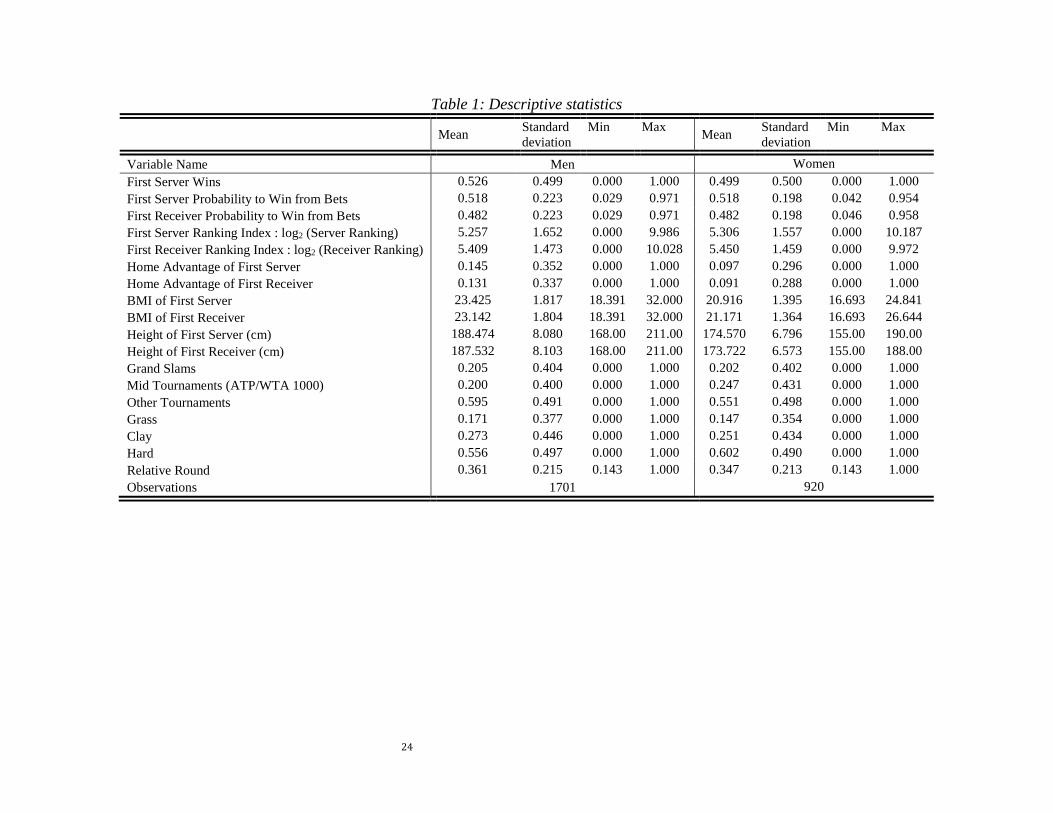
The descriptive statistics of our dataset are presented in Table 1. It shows that, on average,

the player who serves first has a higher probability to win, a better betting odds and a lower

ranking index which is associated with a higher ability. Thus, in order to obtain the causal effect

of serving first, we will use several estimation strategies that control for the positive selection

into treatment (serving first). We discuss these strategies in Section 4.

3.2 Variables

For each match in our dataset, we randomly picked one of the players and denoted him as

Player A and the other player as Player B. Thus, our outcome variable gets the value of one if

Player A won the tiebreak and zero otherwise. In Table 2 we can see that Player A won 50% of

the tiebreaks among men and 50.7% among women.

To estimate the effect of the order of serves, i.e., serving first or second, on performance,

we coded a dummy variable that equals one if Player A served first in the tiebreak and zero

otherwise. Table 2 shows that Player A served first in 49.9% of cases both among men and

women.

11

Our set of controls includes players’ individual characteristics as well as features of

matches and tournaments. In order to control for players’ abilities, based on Klaassen and

Magnus (2001), we use the log2(rank) of players A (RankA) and B (RankB), where Rank is the

most current world ranking of the respective player. We also control for several additional

factors that may be important for winning a point on serve, such as height and BMI (Krumer,

Rosenboim and Shapir, 2016) as well as one of the players having a home advantage (Koning,

2011). The variable that indicates having a home advantage by Player A gets the value of one if

Player A competes at home and Player B does not. Similarly, the variable that indicates having a

home advantage by Player B gets the value of one if he competes at home and Player A does not.

In addition, we also control for type of tournament, surface and the ratio between the round of

the match in the tournament and the total number of rounds.

As we randomized the identity of players A and B, they are not expected to be different in

any of their characteristics. Table 2 compares the means of each characteristic of the two players

and tests whether the difference between them is significant by estimating a univariate regression

of each characteristic as a dependent variable on a dummy variable representing whether the

player is Player A. In Column 3 of Table 2, we report the coefficients of these regressions, where

robust standard errors are in parentheses. We can see that players A and B indeed do not differ in

any of their characteristics, implying that the randomization process was successful. Obviously,

although the identity of Player A is determined randomly, the process which determines which of

the players will serve first in the tiebreak is totally non-random. As we will show in the next

section, due to positive selection into the treatment, serving first is associated with having better

characteristics.

12

4 Estimation strategy

Studying whether serving first in tiebreak gives an advantage to any of the players is a

challenging task. A naïve approach of correlating a dummy variable for serving first with the

probability to win a tiebreak will yield biased and inconsistent estimates because the identity of

the player who serves first is not determined at random. Rather, as mentioned earlier, the winner

of a coin toss gets the privilege to choose whether to serve first or not and his choice may be

based on unobserved characteristics of the two players. Furthermore, isolating an exogenous

source of variation in serving first by using an instrumental variable approach seems unfeasible

because any factor that might be associated with the decision to serve first is also likely to affect

the probability to win the tiebreak.

In the absence of a valid instrument, we will use several alternative strategies to control for

the endogenous choice to serve first. First, we will reduce the amount of selection by adding to a

wide set of controls the probability that gamblers assign to Player A to win the match as reflected

in the betting odds. This is an effective way to reduce selection concerns because many factors

that are unobserved by the researcher are in fact observed by gamblers and are thus captured in

the betting odds. For example, a gambler almost certainly observes factors such as the specific

matchup between the two players, the power of serve, fatigue due to previous competitions,

recent performance, and even weather and temperature conditions.

Second, we utilize fixed effect estimations in which we exploit variation only within a

group of matches where the pre-match betting odds of Player A to win the match are identical.

Thus, within each fixed effect, the relative strength of the two players are kept constant, and thus

the coefficient of serving first can more convincingly be interpreted as causal rather than

reflecting spurious correlations due to omitted factors.

13

Third, we exploit a new methodology that was recently proposed by Oster (2016) for

obtaining a bias-adjusted treatment effect when selection is involved. This methodology follows

Altonji, Elder and Taber (2005) and assesses the bias-adjusted treatment effect under the

assumptions that the amount of selection on unobservables is not greater than the amount of

selection on observables, and that selection on unobservables acts in the same direction as

selection on observables. Thus, if adding the entire set of observed controls to the estimation

moves the coefficient of the treatment variable towards zero then the unobservables will further

push it in this direction. Similarly, if the entire set of observed controls move the coefficient of

interest away from zero then the unobservables are expected to move it even further from zero.

Furthermore, this methodology also extends that of Altonji, Elder and Taber (2005) because it

offers a closed-form estimator of bias under less restrictive assumptions.

Last, we use propensity score matching in which we set the characteristics of the player

who serves first to be equal to the characteristics of the player who receives first. Thus, under the

assumption that the two players are also equal in their unobserved characteristics, the effect of

serving first can be interpreted as causal.

5 Results

5.1 Basic results

We first utilize a cross-section analysis of all the tiebreaks in our dataset in order to

separately estimate by gender a naïve logit model of the probability of Player A to win the

tiebreak as a function of whether or not he/she serves first. Column 1 of Table 3 presents the

results, where Panel A and Panel B report the average marginal effects for men and women,

14

respectively. Robust standard errors appear in parentheses. The results show that serving first is

associated with a 5.1 percentage points higher probability to win the tiebreak among men.

Among women, there is no positive association between serving first and the probability to win

the tiebreak.

However, the causal interpretation of these estimates relies on the assumption that the

players who serve first are, on average, similar in their observed and unobserved characteristics

to the players who receive first, which is unlikely to hold because, as mentioned earlier, serving

first is not determined randomly but rather by choice. Furthermore, selection is also likely to

exist because the performance of the players during the set determines whether at all the set will

reach the tiebreak stage. To provide evidence on the existence of selection, we conduct a balance

test in which, for each gender, we compare the two players in terms of their observed

characteristics. Columns 4 and 5 of Table 2 report the summary statistics of the player who

serves first and the player who receives first, respectively. It can be observed that both among

men and women serving first is positively associated with being the favorite player and having a

lower ranking index (indicating a better player). It is also associated with having a higher height

(which is a clear advantage in tennis), and having a higher pre-match probability to win the

match based on betting odds. In order to examine whether the differences between the two

players are significant we measure the correlation between the serving first variable and each of

our observed controls. Formally, for each of our controls we report the estimate of 1 obtained

from the following model:

ii10i SFX

15

where iX is each of our observed characteristics and iSF is a dummy variable that gets the value

of one if the player serves first, and zero otherwise. The results reported in Column 6 of Table 2

indicate that for both genders the two players differ substantially and significantly in many

observed characteristics. In addition, for men, the player who serves first is associated with

having more favorable characteristics. Thus, since selection into serving first is positive, the

estimates of serving first, presented in Column 1 of Table 3, are likely to be upward-biased.

Indeed, Column 2 indicates that when our set of basic controls is added to the equation, the

coefficient of serving first decreases to 0.027 and becomes insignificant. Among women, the

estimate becomes more negative but is still negligible and very insignificant.

Because these naïve estimates suffer from selection, in the next sections we use the four

different strategies mentioned earlier in order to isolate the pure effect of serving first.

5.2 Controlling for betting odds

In order to reduce the selection concern, in Column 3 of Table 3 we add to our basic set of

controls the probability that Player A wins the match according to the betting odds. In this way,

we are able to control for many factors that are unobserved to the researcher but still observed to

gamblers. As the table indicates, the results show that adding the betting probability to the

estimation hardly has any effect on the coefficient of serving first. This implies that, conditional

on our initial wide set of basic controls, serving first is quite orthogonal to the winning

probabilities that are based on betting odds.

We also check the sensitivity of our estimates to using a linear probability model instead of

logit. The results of these estimations, presented in Columns 4-6, are almost identical to those in

Columns 1-3. In addition, in Table 4, we provide estimates by tournament type, which show that

16

for both men and for women, and for all tournament types, the order of actions in tiebreak does

not provide an advantage to any of the players.

5.3 Oster’s bias-adjusted treatment effect

Next, in order to isolate the selection bias and obtain the bias-adjusted treatment effect of

serving first, we use a formula suggested by Oster (2016), which calculates the bias-adjusted

treatment effect, , as follows:

~/

~]

~[

~ 0

max

0 RRRR

where and 0 are the coefficients of serving first in regressions with and without observed

controls, respectively, and R and 0R are the R-squared values of these regressions, respectively.

The bias-adjusted treatment effect calculated above is conditional on the size of two parameters:

1) the relative degree of selection on observed and unobserved variables ( ) and (2) the R-

squared from a hypothetical regression of the outcome on treatment and both observed and

unobserved controls, maxR . Like Altonji, Elder and Taber (2005), Oster (2016) suggests that

1 may be an appropriate upper bound on . In addition, based on a sample of randomized

papers from top journals, Oster determines that max 1.3R R may be a sufficient upper bound on

maxR . This criterion would allow at least 90% of randomized results to survive. We follow the

bounds on and maxR that Oster suggests, and present in Column 7 of Table 3 the bias-adjusted

treatment effect of serving first. The results show that among men the estimated causal effect

(0.019) is even closer to zero and very insignificant. Among women, the causal effect moves

further from zero but still remains negligible in size and highly insignificant.

17

Oster (2016) also offers an adjusted procedure for evaluating the bias-adjusted treatment

effect when some variables are considered as part of the identification strategy and thus appear

both in the controlled and uncontrolled regressions. The idea is to assess the amount of selection

on the observables conditional on including these variables in the estimation. Because the betting

probability of Player A to win the match captures many observed and unobserved factors that

affect the outcome, it is worthwhile to assess the amount of selection conditional on this variable

being included in the estimation as part of our identification strategy. The results, reported in

Column 8 of Table 3, show that for both men and women the causal effect moves towards zero

and only becomes more insignificant. Thus, all the different specifications in Table 3 indicate

that the order of serves in tiebreak does not provide an advantage to any of the players.

5.4 Fixed-effect estimations

To further reduce the concern of selection, we next estimate fixed effect linear probability

models (LPM) in which we include in each estimation fixed effects for every group of matches

that has the same betting probability of Player A to win the match. In this way, since we use

variation in serving first only within each fixed effect, where the relative strength of the two

players are kept constant, the coefficient of serving first can more convincingly be interpreted as

causal. In these fixed-effect estimations we prefer using a linear probability model rather than

logit because of three main reasons.

First, while this model uses all of the observations, a fixed effect logit model can only use

observations for which the outcome variable varies within each match. Thus, it omits matches in

18

which the outcome is fixed, which may bias the estimates.13 Second, any non-linear estimation

such as logit relies on the functional form while in the linear model the fixed effects account for

variation in the data in a completely general way. Third, a logit fixed effect model yields

consistent estimates only under the stronger assumption of strict exogeneity, while LPM requires

exogeneity to hold only within a fixed effect.

The results of these estimations, by tournament type, are reported in Table 5. Similar to the

results without fixed effects (Table 4), we can see that for both men and for women and for all

types of tournaments, the coefficient of serving first is not significant. Moreover, we also

calculated Oster's bias-adjusted treatment effects for the fixed effect estimation that includes all

the tournaments and find that serving first is far from significant (see Columns 5 and 10, for men

and women, respectively).

5.5 Radius matching analysis

As a last step, we also derive the radius-matching-on-the-propensity-score estimator with

bias adjustment (Lechner, Miquel and Wunsch, 2011). Not only was it found to be very

competitive among a range of propensity score related estimators, but in a later paper Huber,

13 In logit and probit fixed effect models 𝑃𝑟[𝜋𝐴𝑤𝑖𝑛 = 1] = 𝐺[𝛼1 ∙ 𝐴𝑠𝑒𝑟𝑣𝑒 + 𝛽𝑥 + 𝜇𝑚] where .G is the cumulative density

function (CDF) for either the standard normal or the logistic distribution, and 𝜇 is a set of fixed effects for every group of

matches that has the same betting probability of Player A to win the match. It is easy to see that unlike in a linear fixed effect

model, because of the function .G we cannot eliminate m by using within transformation. Moreover, if we attempt to

estimate m directly by adding dummy variables for each match, the estimates of m are inconsistent, and unlike the linear

model, the estimate of 1 becomes inconsistent too. Thus, the only way to obtain a consistent estimate for 1 is to

eliminate m from the equation. In a probit model this is completely impossible. Thus, including fixed effects in a probit

model will yield biased estimates due to the well-known incidental parameter problem (Neyman and Scott, 1948; Greene

2004). Unlike probit models, the logit functional form enables us to eliminate m from the equation but only under the

assumption that the dependent variable changes within each fixed effect. For this reason, it drops matches in which the

outcome is fixed within a given fixed effect.

19

Lechner and Wunsch (2013) actually showed its superior finite sample and robustness properties

in a large scale empirical Monte Carlo study. The main idea of this estimator is to compare

treated and non-treated observations within a specific radius. The first step consists of distance-

weighted radius matching on the propensity score. In contrast to standard matching algorithms

where controls within the radius obtain the same weight independent of their location, in the

radius matching approach, controls within the radius are weighted proportionally to the inverse

of their distance to the respective treated observations they are matched to. The second step uses

the weights obtained from this matching process in a weighted linear or non-linear regression in

order to remove biases due to mismatches. Because this approach uses all comparison

observations within a predefined distance around the propensity score, it allows for higher

precision than fixed nearest neighbour matching in regions in which many similar comparison

observations are available.

We conducted this analysis for two different specifications. In the first specification we

control only for the betting odds, and in the second we also include the basic controls. In Table 6,

we report the results of the propensity score equation. We can see that winning probabilities

based on betting odds are significantly associated with serving first. In addition, selection is also

driven by several physical characteristics. In Table 7 we present the results for the radius

matching estimator. As can be observed, we find no significant effect of serving first on the

probability to win the tiebreak for both men and women. Note that the coefficients and the

standard errors presented in Columns 2 and 4 of Table 7 are generally very similar in size to

those presented in Columns 3 and 6 of Table 3.

20

Taken together, all the estimation strategies above yield the same finding that serving first

in tennis tiebreak does not provide an advantage to any of the players to win the tiebreak, which

implies that the ABBA sequence is quite likely to be fair.

6 Conclusion

The order of actions in contests is a potentially important determinant of performance in

settings ranging from chess matches, penalty shootouts in soccer, or presidential candidate

debates to move into the White House. This paper contributes to the literature by empirically

testing whether the ABBA sequence is fair.

Using several methods that control for selection, we consistently find that there is no

systematic advantage to any player serving first or second in tiebreaks in tennis. In other words,

two-equally skilled players who compete in an ABBA sequence have the same winning

probability. This result applies to both genders and to all types of tournaments.

Our findings, along with evidence on the effect of order of moves on performance in a range

of other environments, suggests that contest designers of sequential tournaments in the areas of

politics, sports, debates, etc., may consider adopting the ABBA sequence if fairness is an

important goal.

7 References

Allouche, J.P. and Shallit, J., 1999. The ubiquitous Prouhet-Thue-Morse sequence. In Sequences

and their applications, pp. 1-16. Springer London.

Altonji, J.G., Elder, T.E. and Taber, C.R., 2005. Selection on observed and unobserved variables:

Assessing the effectiveness of Catholic schools. Journal of Political Economy, 113(1), pp.

151-184.

21

Anderson, C. L., 1977. Note on the advantage of first serve. Journal of Combinatorial Theory,

Series A, 23(3), 363.

Apesteguia, J. and Palacios-Huerta, I., 2010. Psychological pressure in competitive

environments: Evidence from a randomized natural experiment. The American Economic

Review, 100(5), pp. 2548-2564.

Brams, S.J. and Ismail, M.S., 2017. Making the rules of sports fairer. SIAM Review, forthcoming.

Cohen-Zada, D., Krumer, A., Rosenboim, M. and Shapir, O.M., 2017. Choking under pressure

and gender: Evidence from professional tennis. Journal of Economic Psychology, 61, pp. 176-

190.

Cohen-Zada, D. Krumer, A. and Shtudiner, Z., 2017. Psychological momentum and gender.

Journal of Economic Behavior and Organization, 135, pp. 66-81.

De Bruin, W.B., 2005. Save the last dance for me: Unwanted serial position effects in jury

evaluations. Acta Psychologica, 118(3), pp. 245-260.

Echenique, F., 2017. ABAB or ABBA? The arithmetics of penalty shootouts in soccer. Mimeo.

Gauriot, R., and Page, L., 2014. Does success breed success? A quasi-experiment on strategic

momentum in dynamic contests. QUT Business School Discussion paper No. 028.

Genakos, C. and Pagliero, M., 2012. Interim rank, risk taking, and performance in dynamic

tournaments. Journal of Political Economy, 120(4), pp. 782-813.

Genakos, C., Pagliero, M. and Garbi, E., 2015. When pressure sinks performance: Evidence from

diving competitions. Economics Letters, 132, pp. 5-8.

Ginsburgh, V.A. and Van Ours, J.C., 2003. Expert opinion and compensation: Evidence from a

musical competition. The American Economic Review, 93(1), pp. 289-296.

González-Díaz, J., Gossner, O. and Rogers, B.W., 2012. Performing best when it matters most:

Evidence from professional tennis. Journal of Economic Behavior & Organization, 84(3), pp.

767-781.

González-Díaz, J. and Palacios-Huerta, I., 2016. Cognitive performance in competitive

environments: Evidence from a natural experiment. Journal of Public Economics,

forthcoming.

22

Greene, W. (2004). The behavior of the fixed effects estimator in nonlinear models. The

Econometrics Journal, 7(1), 98–119.

Harris, C. and Vickers, J., 1987. Racing with uncertainty. The Review of Economic

Studies, 54(1), pp. 1-21.

Hart, S., 2005. An Interview with Robert Aumann. Macroeconomic Dynamics, 9(05), pp. 683-

740.

Huber, M., Lechner, M. and Steinmayr, A., 2015. Radius matching on the propensity score with

bias adjustment: tuning parameters and finite sample behaviour. Empirical Economics, 49(1),

pp. 1-31.

Huber, M., Lechner, M. and Wunsch, C., 2013. The performance of estimators based on the

propensity score. Journal of Econometrics, 175(1), pp. 1-21.

Kahn, L.M., 2000. The sports business as a labor market laboratory. The Journal of Economic

Perspectives, 14(3), pp. 75-94.

Kingston, J. G., 1976. Comparison of scoring systems in two-sided competitions. Journal of

Combinatorial Theory, Series A, 20(3), pp. 357-362.

Klumpp, T. and Polborn, M.K., 2006. Primaries and the New Hampshire effect. Journal of

Public Economics, 90(6), pp. 1073-1114.

Koning, R.H., 2011. Home advantage in professional tennis. Journal of Sports Sciences, 29(1),

pp. 19-27.

Krumer, A., Rosenboim, M. and Shapir, O.M., 2016. Gender, competitiveness, and physical

characteristics evidence from professional tennis. Journal of Sports Economics, 17(3), pp.

234-259.

Lechner, M., Miquel, R. and Wunsch, C., 2011. Long-run effects of public sector sponsored

training in West Germany. Journal of the European Economic Association, 9(4), pp. 721-784.

Magnus, J.R. and Klaassen, F.J., 1999. On the advantage of serving first in a tennis set: four

years at Wimbledon. Journal of the Royal Statistical Society: Series D (The

Statistician), 48(2), pp. 247-256.

Malueg, D.A. and Yates, A.J., 2010. Testing contest theory: evidence from best-of-three tennis

matches. The Review of Economics and Statistics, 92(3), pp. 689-692.

23

Neyman, J., and Scott, E. L. (1948). Consistent estimates based on partially consistent

observations. Econometrica: Journal of the Econometric Society, 16(1), pp. 1-32.

Oster, E., 2016. Unobservable selection and coefficients stability: Theory and Evidence. Journal

of Businnes Economics and Statistics, forthcoming.

Page, L. and Page, K., 2010. Last shall be first: A field study of biases in sequential performance

evaluation on the Idol series. Journal of Economic Behavior & Organization, 73(2), pp. 186-

198.

Page, L. and Coates, J., 2017. Winner and loser effects in human competitions. Evidence from

equally matched tennis players. Evolution and Human Behavior, forthcoming.

Palacios-Huerta. I., 2012. Tournaments, fairness and the Prouhet‐Thue‐Morse sequence.

Economic Inquiry, 50(3), pp. 848-849.

Palacios-Huerta, I., 2014. Psychological pressure on the field and elsewhere. Chapter 5

in Beautiful game theory: How soccer can help economics. Princeton University Press.

Palacios-Huerta, I. and Volij, O., 2009. Field centipedes. The American Economic Review, 99(4),

pp. 1619-1635.

Rosen, S., 1986. Prizes and incentives in elimination tournaments. The American Economic

Review, 76(4), pp. 701-715.

Szymanski, S., 2003. The economic design of sporting contests. Journal of Economic

Literature, 41(4), pp. 1137-1187.

Thue, A., 1912. Uber unendliche Zeichenreihen. Kra. Vidensk. Selsk. Skrifter. I. Mat.-Nat.,

Christiana, 10. Reprinted in Selected Mathematical Papers of Axel Thue, edited by T. Nagell.

Oslo: Universitetsforlaget, 1977, pp. 139–158.

24

Table 1: Descriptive statistics

Mean Standard

deviation

Min Max Mean

Standard

deviation

Min Max

Variable Name Men Women

First Server Wins 0.526 0.499 0.000 1.000 0.499 0.500 0.000 1.000

First Server Probability to Win from Bets 0.518 0.223 0.029 0.971 0.518 0.198 0.042 0.954

First Receiver Probability to Win from Bets 0.482 0.223 0.029 0.971 0.482 0.198 0.046 0.958

First Server Ranking Index : log2 (Server Ranking) 5.257 1.652 0.000 9.986 5.306 1.557 0.000 10.187

First Receiver Ranking Index : log2 (Receiver Ranking) 5.409 1.473 0.000 10.028 5.450 1.459 0.000 9.972

Home Advantage of First Server 0.145 0.352 0.000 1.000 0.097 0.296 0.000 1.000

Home Advantage of First Receiver 0.131 0.337 0.000 1.000 0.091 0.288 0.000 1.000

BMI of First Server 23.425 1.817 18.391 32.000 20.916 1.395 16.693 24.841

BMI of First Receiver 23.142 1.804 18.391 32.000 21.171 1.364 16.693 26.644

Height of First Server (cm) 188.474 8.080 168.00 211.00 174.570 6.796 155.00 190.00

Height of First Receiver (cm) 187.532 8.103 168.00 211.00 173.722 6.573 155.00 188.00

Grand Slams 0.205 0.404 0.000 1.000 0.202 0.402 0.000 1.000

Mid Tournaments (ATP/WTA 1000) 0.200 0.400 0.000 1.000 0.247 0.431 0.000 1.000

Other Tournaments 0.595 0.491 0.000 1.000 0.551 0.498 0.000 1.000

Grass 0.171 0.377 0.000 1.000 0.147 0.354 0.000 1.000

Clay 0.273 0.446 0.000 1.000 0.251 0.434 0.000 1.000

Hard 0.556 0.497 0.000 1.000 0.602 0.490 0.000 1.000

Relative Round 0.361 0.215 0.143 1.000 0.347 0.213 0.143 1.000

Observations 1701 920

25

Table 2: Selection into treatment

Random Player A Random Player B Difference First Server First Receiver Difference

(1) (2) (3) (4) (5) (6)

Panel A: Men’s tournaments

Share of Wins 0.500

(0.500)

0.500

(0.500)

-0.001

(0.017)

0.526

(0.499)

0.474

(0.499)

0.051***

(0.017)

Betting Odds (prob. to win) 0.498

(0.224)

0.502

(0.224)

-0.005

(0.008)

0.518

(0.223)

0.482

(0.223)

0.036***

(0.008)

First Server 0.499

(0.500)

0.501

(0.500)

-0.002

(0.017)

Ranking Index: log2 Rank 5.335

(1.530)

5.330

(1.603)

0.005

(0.054)

5.257

(1.652)

5.409

(1.473)

-0.152***

(0.054)

Home Advantage 0.005

(0.465)

-0.005

(0.465)

0.011

(0.016)

0.015

(0.464)

-0.015

(0.464)

0.029*

(0.016)

BMI 23.270

(1.777)

23.297

(1.854)

-0.027

(0.062)

23.425

(1.817)

23.142

(1.804)

0.283***

(0.062)

Height 1.878

(0.080)

1.882

(0.082)

-0.003

(0.003)

1.885

(0.081)

1.875

(0.081)

0.009***

(0.003)

Favorite 0.509

(0.500)

0.491

(0.500)

0.017

(0.017)

0.537

(0.499)

0.463

(0.499)

0.073***

(0.017)

Panel B: Women’s tournaments

Share of wins 0.507

(0.500)

0.493

(0.500)

0.013

(0.023)

0.499

(0.500)

0.501

(0.500)

-0.002

(0.023)

Betting Odds (prob. to win) 0.496

(0.198)

0.504

(0.198)

-0.009

(0.009)

0.518

(0.198)

0.482

(0.198)

0.036***

(0.009)

First Server 0.499

(0.500)

0.501

(0.500)

-0.002

(0.023)

Ranking Index: log2 Rank 5.366

(1.514)

5.390

(1.507)

-0.024

(0.070)

5.306

(1.557)

5.450

(1.459)

-0.144**

(0.070)

Home Advantage 0.001

(0.408)

-0.001

(0.408)

0.002

(0.019)

0.005

(0.408)

-0.005

(0.408)

0.011

(0.019)

BMI 21.016

(1.387)

21.071

(1.384)

-0.055

(0.065)

20.916

(1.395)

21.171

(1.364)

-0.254***

(0.064)

Height 1.744

(0.066)

1.739

(0.067)

0.005

(0.003)

1.746

(0.068)

1.737

(0.066)

0.008***

(0.003)

Favorite 0.502

(0.500)

0.498

(0.500)

0.004

(0.023)

0.521

(0.500)

0.479

(0.500)

0.041*

(0.023)

26

Table 3: The effect of serving first on the probability to win the tiebreak

Logit Regression LPM Oster

(1) (2) (3) (4) (5) (6) (7) (8) Panel A: Men’s tournaments

Player A Serves First 0.051** 0.027 0.027 0.051** 0.028 0.027 0.019 0.012

(0.024) (0.024) (0.024) (0.024) (0.024) (0.024) (0.024) (0.025)

Number of obs. 1,701 1,701 1,701 1,701 1,701 1,701 1,701 1,701

Panel B: Women’s tournaments

Player A Serves First -0.002 -0.007 -0.008 -0.002 -0.007 -0.008 -0.010 -0.007

(0.033) (0.033) (0.033) (0.033) (0.033) (0.033) (0.033) (0.032)

Number of obs. 920 920 920 920 920 920 920 920

Player A prob. to win

based on betting odds

N N Y N N Y Y Y

Basic controls N Y Y N Y Y Y Y

Note: The list of basic controls includes the ranking indexes of players A and B, whether each of the players has

a home advantage, the height and BMI index of each player, the round of the match in the tournament relative to

the total number of rounds, as well as type of tournament- and surface-fixed effects. In Column 7 we report

Oster's bias-adjusted treatment effect when the amount of selection on unobservables is recovered from the

amount of selection on all observables. In Column 8 we treat the betting odds as part of the identification

strategy and thus recover the amount of selection on unobservables from the amount of selection on all the other

observed characteristics, where the betting odds is included both in the controlled and uncontrolled regressions.

Robust standard errors are presented in parentheses. Standard errors in columns 7 and 8 are obtained from

bootstrapping (500 replications). *, **, *** denote significance at the 10%, 5%, 1% level respectively.

27

Table 4:

Logit estimates of the effect of serving first on the probability to win the tiebreak

Men’s tournaments Women’s tournaments

Variable Small

tourn.

ATP

1000

Grand-

Slams

All

tourn.

Small

tourn.

WTA

1000

Grand-

Slams

All

tourn.

(1) (2) (3) (4) (5) (6) (7) (8)

Player A Serves First 0.028 -0.006 0.053 0.027 0.007 0.000 -0.037 -0.008

(0.031) (0.054) (0.052) (0.024) (0.044) (0.067) (0.074) (0.033)

Number of Obs. 1,012 341 348 1,701 507 227 186 920

Note: In all the regressions we control for Player A’s winning probability based on betting odds, the ranking index of players A and B, whether each of them has a

home advantage, their height and BMI index, the round of the match in the tournament relative to the total number of rounds as well as type of tournament- and

surface-fixed effects. Robust standard errors are presented in parentheses. *, **, *** denote significance at the 10%, 5%, 1% level respectively.

Table 5:

Fixed effects estimation of the effect of serving first on the probability to win the tiebreak

Men’s tournaments Women’s tournaments

Variable Small

tourn.

ATP

1000

Grand-

Slams

All

tourn.

Oster Small

tourn.

WTA

1000

Grand-

Slams

All

tourn.

Oster

(1) (2) (3) (4) (5) (6) (7) (8) (9) (10)

Player A Serves First 0.037

(0.034)

0.009

(0.069)

0.059

(0.061)

0.029

(0.024)

0.003

(0.029)

0.042

(0.057)

-0.033

(0.079)

0.007

(0.135)

-0.010

(0.041)

0.013

(0.033)

Number of Obs. 1,012 341 348 1,701 1,701 507 227 186 920 920

Number of Groups 99 81 95 125 125 87 69 81 116 116

Note: In all the regressions we control for Player A’s winning probability based on betting odds, the ranking index of players A and B, whether each of them has a

home advantage, their height and BMI index, the round of the match in the tournament relative to the total number of rounds as well as type of tournament- and

surface-fixed effects. Robust standard errors are presented in parentheses. Standard errors in columns 5 and 10 are obtained from bootstrapping (500 replications). *,

**, *** denote significance at the 10%, 5%, 1% level, respectively.

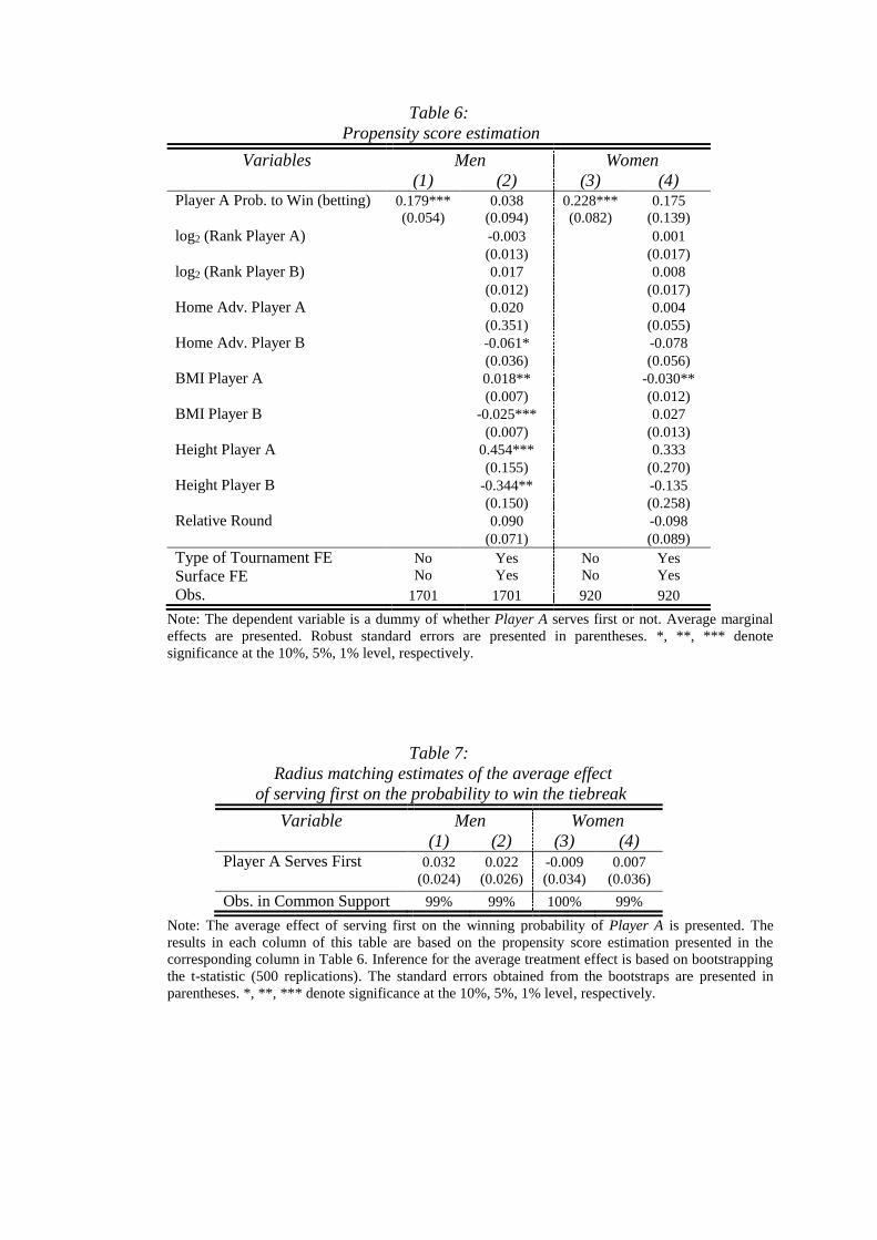
Table 6:

Propensity score estimation

Variables Men Women

(1) (2) (3) (4) Player A Prob. to Win (betting) 0.179*** 0.038 0.228*** 0.175

(0.054) (0.094) (0.082) (0.139)

log2 (Rank Player A) -0.003 0.001

(0.013) (0.017)

log2 (Rank Player B) 0.017 0.008

(0.012) (0.017)

Home Adv. Player A 0.020 0.004

(0.351) (0.055)

Home Adv. Player B -0.061* -0.078

(0.036) (0.056)

BMI Player A 0.018** -0.030**

(0.007) (0.012)

BMI Player B -0.025*** 0.027

(0.007) (0.013)

Height Player A 0.454*** 0.333

(0.155) (0.270)

Height Player B -0.344** -0.135

(0.150) (0.258)

Relative Round 0.090 -0.098

(0.071) (0.089)

Type of Tournament FE No Yes No Yes

Surface FE No Yes No Yes

Obs. 1701 1701 920 920

Note: The dependent variable is a dummy of whether Player A serves first or not. Average marginal

effects are presented. Robust standard errors are presented in parentheses. *, **, *** denote

significance at the 10%, 5%, 1% level, respectively.

Table 7:

Radius matching estimates of the average effect

of serving first on the probability to win the tiebreak

Variable Men Women

(1) (2) (3) (4) Player A Serves First 0.032 0.022 -0.009 0.007

(0.024) (0.026) (0.034) (0.036)

Obs. in Common Support 99% 99% 100% 99%

Note: The average effect of serving first on the winning probability of Player A is presented. The

results in each column of this table are based on the propensity score estimation presented in the

corresponding column in Table 6. Inference for the average treatment effect is based on bootstrapping

the t-statistic (500 replications). The standard errors obtained from the bootstraps are presented in

parentheses. *, **, *** denote significance at the 10%, 5%, 1% level, respectively.