diurnal cycle of surface winds over the subtropical

Diurnal cycle of surface winds over the subtropical

southeast Pacific

R. C. Munoz1

Received 12 February 2008; revised 12 April 2008; accepted 30 April 2008; published 3 July 2008.

[1] The diurnal variability of surface winds over the SE Pacific is characterized withQuikSCAT data for years 2000–2006. The twice daily satellite passes occur around0600 and 1800 LT (referred to as AM and PM, respectively). The PM-AM wind differencemaximizes in a region between 20�S and 30�S, extending from the Chilean coast upto 75�W. This difference is mostly meridional (along the coast) with seasonal variationcharacterized by summertime weakening of the morning winds. The observationalanalysis is supplemented with mesoscale model results for December 2003. Theyshow that the coastal zonal flow increases between 0600 and 1200 local time (LT) butthen decreases in the next 6 hours, which explains the absence of an onshore componentin the QuikSCAT PM-AM difference. Additional model diagnostics show that in thisregion the diurnal cycle hodographs are more simple and larger above the marineboundary layer (MBL) than at the surface. Evaluation of the momentum and temperaturebudgets reveals the importance of the diurnal cycle of vertical velocity coupled withthe thermal structure in controlling the diurnal cycle of the low-level winds. Around1300 LT coastal subsidence maximizes in a layer sloping from 1000 m at 36�S to 3000 mat 22�S, inducing the development of a coastal trough at the surface. During the nightthe passage of a high-pressure perturbation reverses the surface meridional pressuregradient force, inducing the decrease of the coastal meridional winds. These results stressthe important role played by the dynamics of the low troposphere above the MBL(e.g., the heating of the Andes Cordillera to the east) in controlling the wind diurnalcycles near the surface.

Citation: Munoz, R. C. (2008), Diurnal cycle of surface winds over the subtropical southeast Pacific, J. Geophys. Res., 113, D13107,

doi:10.1029/2008JD009957.

1. Introduction

[2] The southeast (SE) Pacific region off north centralChile (19�–35�S, 80�–70�W) is a region of considerableclimatic interest. It encompasses a subtropical anticyclonethat maintains an extensive and persistent deck of low-level stratocumulus (Sc) clouds which have a large impacton the planetary radiative budget [Hartmann et al., 1992].To the east, the region is bounded by topography rising inless than 200 km from sea level to the peaks of the AndesCordillera (heights >4000 m), leaving in between the ex-tremely arid Atacama Desert. In previous work we havepresented data analysis [Garreaud and Munoz, 2005] andnumerical modeling results [Munoz and Garreaud, 2005]aimed at describing and understanding a low-level windmaximum which exists along the eastern border of thesubtropical SE Pacific region. The present work extendsthe study into the diurnal cycle of low-level winds in thesame region.[3] The diurnal variability of low-level clouds in this

geographical area has already been shown to be relatively

large [e.g., Rozendaal et al., 1995], and, although we do notdwell on this matter here, we may presume that diurnalvariations of winds and clouds are well related dynamicallyand thermodynamically. In fact, for a geographical settingsimilar to the one considered in this work, Koracin andDorman [2001] showed that off the California coast thediurnal variation of the nearshore cloudiness is highlycoupled to the convergence and divergence of the low-levelwinds. More generally, right at the coast a band of after-noon clearing and onshore wind acceleration are well-known features of sea breeze circulations [e.g., Simpson,1994, p. 21] that may be important to explain the diurnalcycles in the SE Pacific region. However, the complextopography in this area, among other factors, can certainlycomplicate the way that the sea breeze takes form.[4] Besides their expected interaction with the low-level

cloudiness, the diurnal variability of low-level winds mayalso impact the oceanic circulation. Near the coast, forexample, the nocturnal weakening of the winds induces asignificant surface stress rotor important in the maintenanceof coastal upwelling of deeper waters [Rutllant et al., 2004].Lerczak et al. [2001] show evidence of diurnal variability insubsurface currents that may be related to the diurnalcomponent of the surface wind variability.

JOURNAL OF GEOPHYSICAL RESEARCH, VOL. 113, D13107, doi:10.1029/2008JD009957, 2008ClickHere

for

FullArticle

1Department of Geophysics, University of Chile, Santiago, Chile.

Copyright 2008 by the American Geophysical Union.0148-0227/08/2008JD009957$09.00

D13107 1 of 15

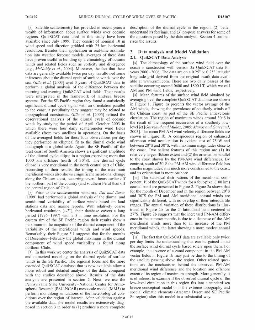
http://dx.doi.org/10.1029/2008JD009957

[5] Satellite scatterometry has provided in recent years awealth of information about surface winds over oceanicregions. QuikSCAT data used in this study have beenavailable since July 1999. They consist of nominal 10 mwind speed and direction gridded with 25 km horizontalresolution. Besides their application in real-time assimila-tion into weather forecast models, averages of these datahave proven useful in building up a climatology of oceanicwinds and related fields such as vorticity and divergence[e.g., McNoldy et al., 2004]. Moreover, the fact that thesedata are generally available twice per day has allowed someinferences about the diurnal cycle of surface winds over thesea. Gille et al. [2003] used 3 years of QuikSCAT data toperform a global analysis of the difference between themorning and evening QuikSCAT wind fields. Their resultswere interpreted in the framework of land/sea breezesystems. For the SE Pacific region they found a statisticallysignificant diurnal cycle signal with an orientation parallelto the coast, a peculiarity they suggest may be related totopographical constraints. Gille et al. [2005] refined theobservational analysis of the diurnal cycle of oceanicwinds by studying the period of April–October 2003 inwhich there were four daily scatterometer wind fieldsavailable (from two satellites in operation). On the basisof the averaged fields for these four observations per daythey performed an elliptical fit to the diurnal cycle windhodograph at a global scale. Again, the SE Pacific off thewest coast of South America shows a significant amplitudeof the diurnal cycle ellipse in a region extending more that1000 km offshore (north of 30�S). The diurnal cycleellipse is very meridional in the north central part of Chile.According to their results, the timing of the maximummeridional winds also shows a significant meridional changealong the Chilean coast, occurring several hours earlier offthe northern part of the country (and southern Peru) than offthe central region of Chile.[6] Prior to the scatterometer wind era, Dai and Deser

[1999] had performed a global analysis of the diurnal andsemidiurnal variability of surface winds based on landstations data and marine reports. With relatively coarsehorizontal resolution (�2�), their database covers a longperiod (1976–1997) with a 3 h time resolution. For theeastern rim of the SE Pacific region their results show amaximum in the magnitude of the diurnal component of thevariability of the meridional winds and wind speeds.Remarkably, their Figure 5.1 suggests that for the monthsof December–February the global maximum in the diurnalcomponent of wind speed variability is found alongnorthern Chile.[7] In this work we center the analysis of QuikSCAT data

and numerical modeling on the diurnal cycle of surfacewinds in the SE Pacific. The regional focus and the moreextended QuikSCAT database that is now available allow amore robust and detailed analysis of the data, comparedwith the studies described above. Results of the dataanalysis are presented in section 2. Next, we use thePennsylvania State University–National Center for Atmo-spheric Research (PSU-NCAR) mesoscale model (MM5) toperform monthlong simulations of the meteorological con-ditions over the region of interest. After validation againstthe available data, the model results are extensively diag-nosed in section 3 in order to (1) produce a more complete

description of the diurnal cycle in the region, (2) betterunderstand its forcings, and (3) propose answers for some ofthe questions posed by the data analysis. Section 4 summa-rizes the results.

2. Data analysis and Model Validation

2.1. QuikSCAT Data Analysis

[8] The climatology of the surface wind field over theocean is constructed with version 3a QuikSCAT data foryears 2000–2006. The data are on a 0.25� � 0.25� latitude/longitude grid derived from the original swath data avail-able at www.ssmi.com. There are two daily passes of thesatellite occurring around 0600 and 1800 LT, which we callAM and PM wind fields, respectively.[9] Mean features of the surface wind field obtained by

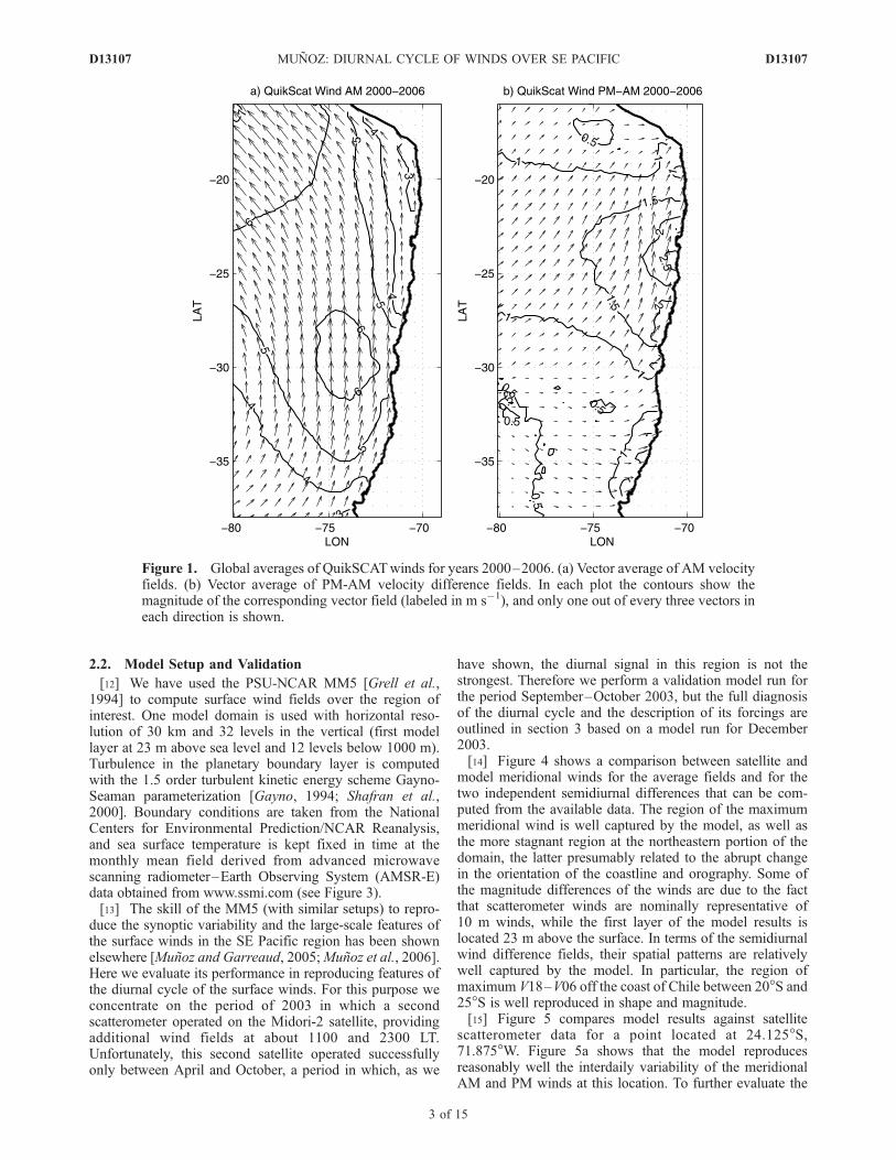
averaging over the complete QuikSCAT database are shownin Figure 1. Figure 1a presents the vector average of theAM winds, showing the prevalence of southerly winds offthe Chilean coast, as part of the SE Pacific anticycloniccirculation. The region of maximum winds around 30�S isthe result of the frequent occurrence of a southerly low-level jet [Garreaud and Munoz, 2005;Munoz and Garreaud,2005]. The mean PM-AMwind velocity difference fields areshown in Figure 1b. A conspicuous region of enhancedafternoon wind acceleration is evident east of 75�W andbetween 20�S and 30�S, with maximum magnitudes close tothe coast. Two salient features of this region are (1) itsrelatively large offshore extent and (2) the orientation parallelto the coast shown by the PM-AM wind differences. Bycontrast, south of 30�S the PM-AMwind difference field hassmaller magnitudes; it is much more constrained to the coast,and its orientation is more onshore.[10] The statistical distributions of the meridional com-

ponent, V, of the QuikSCATwinds for a four-pixel (100 km)coastal band are presented in Figure 2. Figure 2a shows thatfor the month of December and in the region between 20�Sand 30�S the PM and AM meridional coastal winds aresignificantly different, with no overlap of their interquartileranges. The annual variation of these distributions is illus-trated in Figure 2b for the 2� latitudinal band centered at27�S. Figure 2b suggests that the increased PM-AM differ-ence in the summer months is due to a decrease of the AMmeridional winds more than to an increase of the PMmeridional winds, the latter showing a more modest annualcycle.[11] The fact that QuikSCAT data are available only twice

per day limits the understanding that can be gained aboutthe surface wind diurnal cycle based solely upon them. Forexample, the absence of a zonal component in the PM-AMvector fields in Figure 1b may just be due to the timing ofthe satellite passing above the region. Other related ques-tions are the mechanisms behind the observed PM-AMmeridional wind difference and the location and offshoreextent of its region of maximum strength. More generally, itis of interest to examine if the observed diurnal cycle of thelow-level circulation in this region fits into a standard seabreeze conceptual model or if the extreme topography andspecial climatic elements (Atacama Desert and SE PacificSc region) alter this model in a substantial way.

D13107 MUNOZ: DIURNAL CYCLE OF WINDS OVER SE PACIFIC

2 of 15

D13107

2.2. Model Setup and Validation

[12] We have used the PSU-NCAR MM5 [Grell et al.,1994] to compute surface wind fields over the region ofinterest. One model domain is used with horizontal reso-lution of 30 km and 32 levels in the vertical (first modellayer at 23 m above sea level and 12 levels below 1000 m).Turbulence in the planetary boundary layer is computedwith the 1.5 order turbulent kinetic energy scheme Gayno-Seaman parameterization [Gayno, 1994; Shafran et al.,2000]. Boundary conditions are taken from the NationalCenters for Environmental Prediction/NCAR Reanalysis,and sea surface temperature is kept fixed in time at themonthly mean field derived from advanced microwavescanning radiometer–Earth Observing System (AMSR-E)data obtained from www.ssmi.com (see Figure 3).[13] The skill of the MM5 (with similar setups) to repro-

duce the synoptic variability and the large-scale features ofthe surface winds in the SE Pacific region has been shownelsewhere [Munoz and Garreaud, 2005;Munoz et al., 2006].Here we evaluate its performance in reproducing features ofthe diurnal cycle of the surface winds. For this purpose weconcentrate on the period of 2003 in which a secondscatterometer operated on the Midori-2 satellite, providingadditional wind fields at about 1100 and 2300 LT.Unfortunately, this second satellite operated successfullyonly between April and October, a period in which, as we

have shown, the diurnal signal in this region is not thestrongest. Therefore we perform a validation model run forthe period September–October 2003, but the full diagnosisof the diurnal cycle and the description of its forcings areoutlined in section 3 based on a model run for December2003.[14] Figure 4 shows a comparison between satellite and

model meridional winds for the average fields and for thetwo independent semidiurnal differences that can be com-puted from the available data. The region of the maximummeridional wind is well captured by the model, as well asthe more stagnant region at the northeastern portion of thedomain, the latter presumably related to the abrupt changein the orientation of the coastline and orography. Some ofthe magnitude differences of the winds are due to the factthat scatterometer winds are nominally representative of10 m winds, while the first layer of the model results islocated 23 m above the surface. In terms of the semidiurnalwind difference fields, their spatial patterns are relativelywell captured by the model. In particular, the region ofmaximum V18–V06 off the coast of Chile between 20�S and25�S is well reproduced in shape and magnitude.[15] Figure 5 compares model results against satellite

scatterometer data for a point located at 24.125�S,71.875�W. Figure 5a shows that the model reproducesreasonably well the interdaily variability of the meridionalAM and PM winds at this location. To further evaluate the

Figure 1. Global averages of QuikSCATwinds for years 2000–2006. (a) Vector average of AM velocityfields. (b) Vector average of PM-AM velocity difference fields. In each plot the contours show themagnitude of the corresponding vector field (labeled in m s�1), and only one out of every three vectors ineach direction is shown.


3 of 15

D13107

model with respect to the diurnal variation of the merid-ional winds, Figure 5b shows the anomalies with respectto the daily mean based on model results and scatterometerwinds for the 25 days in the period in which all foursatellite passes were available at this point. The modelreproduces well the tendency in the observations of havingreduced meridional winds at the end of the night and inthe morning and increased magnitudes and variability bylate afternoon.

3. Diurnal Cycle Characterization

3.1. Assessing the QuikSCAT Timing Effect

[16] Model results for December 2003 are used here tobuild a more complete picture of the diurnal cycle of thelow-level winds over the SE Pacific. In what follows, UTCminus 5 h will be used as local time (LT) for describingmodel results. Figure 6 addresses the question of why thePM-AM zonal wind difference in the QuikSCAT data is sosmall. We have plotted there the mean 6-hourly changes inzonal (Figures 6a–6d) and meridional (Figures 6e–6h)winds. Figure 6b shows that there is indeed an increase inthe zonal winds along a coastal band between 0600 and1200 LT, but in the next 6 hours they experience acomparable decrease in magnitude. The net result for the

0600–1800 LT period (similar to the integration period ofthe QuikSCAT data) is only a very modest mean variationof the zonal wind.[17] Figures 6e–6h show the corresponding 6-hourly

changes of the meridional wind. In the 0600–1800 LTperiod (Figures 6f and 6g) the coastal band off north centralChile shows a relatively persistent increase of this windcomponent, explaining the larger values of the PM-AMmeridional wind difference captured by the QuikSCATdata. On the other hand, during the nocturnal phase of thediurnal cycle (Figures 6e and 6h) the meridional windchanges in the SE Pacific appear to be highly related tothe surface pressure perturbation induced by the ‘‘upsidencewave’’ feature described by Garreaud and Munoz [2004].From the results above we conclude that the picture givenby the QuikSCAT data of the diurnal cycle of the surfacewinds in this region may indeed be affected by the timingof the satellite passes and its relation with the phases of thedaytime heating and the propagation of the upsidence waveperturbation during the night.

3.2. Diurnal Cycle Hodographs

[18] The average wind diurnal cycle hodographs com-puted by the model are shown in Figure 7 for the layer at23 m (Figure 7a) and for that at 1404 m (Figure 7b) (the

Figure 2. Statistical box plots of coastal meridional winds based on QuikSCAT data for years 2000–2006. The boxes define the interquartile range of each distribution, and the horizontal line marks itsmedian. Open boxes correspond to AM data, and shaded boxes correspond to PM data. The four datapixels closest to the coast are considered coastal, and the data have been binned in 2� latitudinal bands.(a) Latitudinal variation of coastal meridional wind distributions for the month of December. (b) Annualvariation of coastal meridional wind distributions for the 2� region around 27�S.


4 of 15

D13107

mean wind vector has been subtracted at each point). Theamplitude of the diurnal cycle hodographs at the surface islarger at the grid points closer to the Chilean coast, comparedwith grid points offshore. The structure of these coastalhodographs, however, can be quite complex. For example,between 20�S and 30�S the zonal wind diurnal cycle near thecoast exhibits a double cycle in its diurnal variation givingthe hodograph a characteristic ‘‘figure eight’’ form. South of30�S the coastal hodographs are more like what may beexpected for a simple coastal circulation driven by the land-sea temperature difference and the Coriolis effect.[19] Figure 7b shows the diurnal cycle hodographs for a

model layer well above the marine boundary layer (MBL).In a region between 20�S and 30�S and extending about500 km offshore, the diurnal cycle hodographs are signif-icantly ‘‘larger’’ above the MBL than at the surface. Theyare also much simpler, an indication that the double cycle inthe zonal wind variation described above is a near-surfacefeature. South of 30�S the amplitude of the diurnal cyclehodographs at this level is very small.[20] These model results suggest that north of 30�S the

larger amplitudes of the wind diurnal cycles are found

above the MBL, while those near the surface presentconsiderable complexity. In contrast, south of 30�S thediurnal cycles are larger in the MBL than above and areimportant in a region more constrained to the coast. Partialobservational support of these results is given by Rutllant etal. [2003], who describe significant diurnal cycles of wind,temperature, and mixing ratio in a layer extending from1000 to 4000 m above sea level according to rawinsondemeasurements carried out at 23�S.

3.3. Diurnal Cycle Forcings

[21] Figure 8a shows the mean diurnal cycle of themeridional wind, V, at a point located at 25.93�S,72.48�W for the region between the surface and 3000 m.Maximum meridional winds are found at about 600 m(top of the modeled MBL), reaching mean values over14 m s�1 between 1800 and 2200 LT. Figure 8b shows thetime rate of change of the meridional wind. The diurnalcycle of V has larger amplitudes in the region below2000 m, with maximum decelerations (@V/@t < 0, wheret is time) around 0100 LT and maximum accelerations(@V/@t > 0) between 1300 and 1600 LT. Below 1000 m

Figure 3. Sea surface temperature (SST) (line contours in �C) used in model run for September–October 2003. Shaded contours (meters above sea level) correspond to the topography of the model.

Figure 4. Comparison of satellite scatterometer winds and MM5 results for September–October 2003. (a) Meanmeridional wind at 1800 LT from QuikSCAT. (b) As in Figure 4a but for MM5 results. (c) Average difference of meridionalwinds between 1800 and 0600 LT satellite passes. (d) As in Figure 4c but for MM5 results. (e) Average difference ofmeridional winds between 2300 and 1100 LT satellite passes. (f ) As in Figure 4e but for MM5 results.


5 of 15

D13107

Figure 4


6 of 15

D13107

Figure 5. Comparison of model results and QuikSCAT data for point located at 24.125�S, 71.875�Wfor September–October 2003. (a) Meridional winds at AM (circles) and PM (crosses) satellite passes.(b) Meridional wind diurnal anomalies from satellite scatterometer data (circles) and from MM5 results.Only 25 days with four satellite data per day are shown.

Figure 6. Averaged 6-hourly changes of (a–d) zonal and (e–h) meridional winds computed from MM5results for December 2003. Shaded contours represent positive changes, and dashed contours representnegative changes. Contour values are in m s�1 (the zero contour has been omitted).


7 of 15

D13107

the values of V increase continuously between 0700 and1700 LT, reaching maximum values between 1700 and1900 LT. The diagnosis of all forcings in the meridionalmomentum budget shows that the main factor responsiblefor this acceleration is the meridional pressure gradientforce (PGF), whose mean time-height structure is shown inFigure 8c. Above 2000 m the mean meridional PGF at thispoint remains negative all day, consistent with a westerlygeostrophic wind. Below 2000 m, however, the PGF ispositive most of the day, maximizing at the surface at1000–1300 LT and becoming negative between 2300 and0500 LT. The latter feature is responsible for the nocturnaldeceleration of the low-level meridional wind in thisregion, which, as we showed in section 3.1, is an impor-tant part of its diurnal cycle.[22] The modeled mean diurnal cycle of surface pressure

along the coast is shown in Figure 9. The coastal surfacepressure has a relatively large diurnal cycle in the region

north of 30�S. In northern Chile (18�–22�S), minimumsurface pressures occur between 1300 and 1600 LT, andmaximum values occur at about 0100 LT. Although thetiming of the minimum coastal pressure does not vary muchlatitudinally, the timing of the maximum surface pressureoccurs about 6 h later at 30�S than at 20�S. The structure ofthe diurnal pressure cycle in Figure 9 shows that thepressure gradient along the coast maximizes its diurnalcycle in the transition region between 30�S and 22�S, whereit even reverses sign during the nocturnal phase.[23] Now we address the factors explaining the diurnal

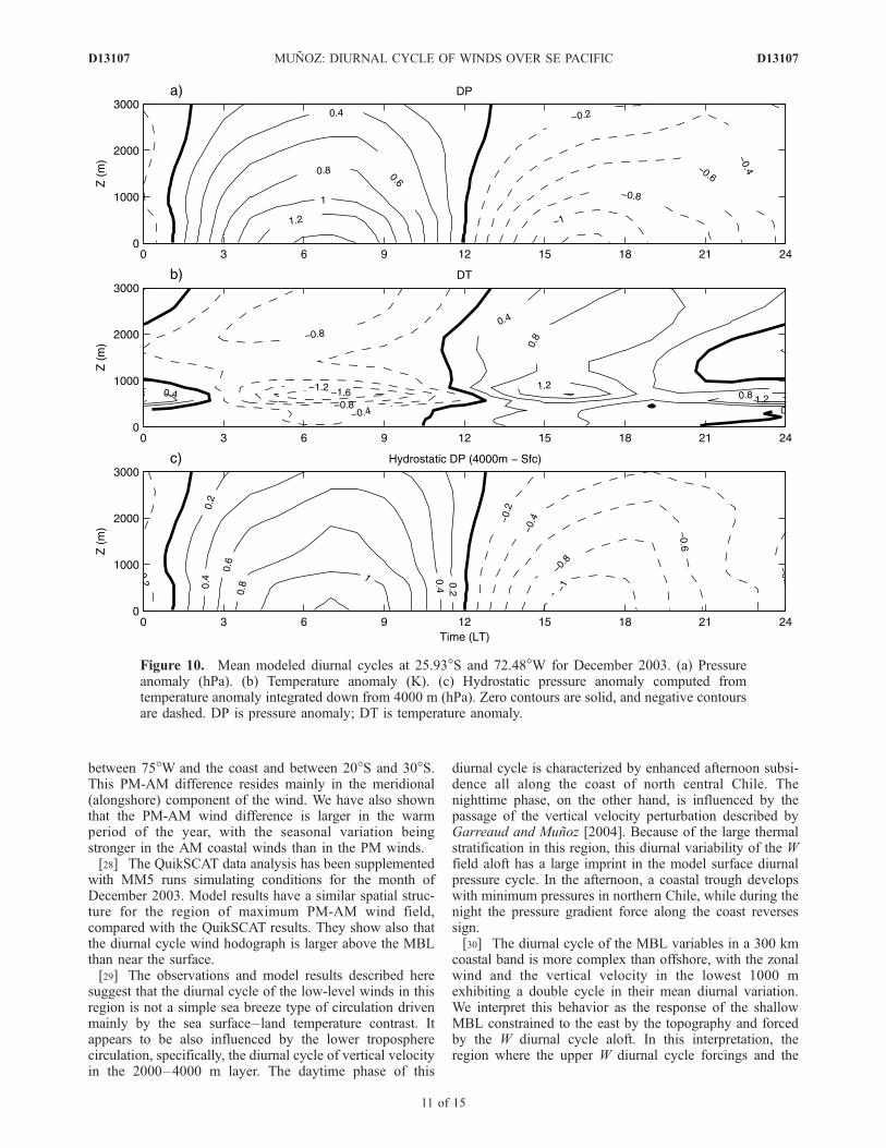
cycle of surface pressure in the model results. Figure 10ashows a time-height cross section of pressure anomaliescomputed by subtracting at each level the pressure averagedover the full modeling period. The diurnal pressure cyclehas a very clear pattern with maximum magnitudes at thesurface, maximum pressures around 0700 LT, and mini-mum values around 1600 LT. In turn, this diurnal pressure

Figure 7. Mean diurnal cycle hodographs computed from MM5 results for December 2003. The meanwind vector for each point has been subtracted from the hodographs. Crosses mark the grid pointcorresponding to each hodograph (one out of every six model grid points is shown). Hodographs begin at0100 LT and end at 2400 LT, and a dot marks the 1800 LT point. In the top right corner there is areference hodograph with a 2 m s�1 radius. (a) Diurnal cycle hodographs for 23 m. (b) As in Figure 7abut for 1404 m.


8 of 15

D13107

cycle is largely explained by the diurnal variation in thetemperature profile. Indeed, Figure 10b shows the diurnalcycle of temperature anomalies, which has a more complexstructure and presents large magnitudes at the subsidenceinversion level. These temperature anomalies have beenhydrostatically converted into pressure perturbations (usinga reference density of 1 kg m�3) and then integrated from4000 m down to each level to produce the pattern shown inFigure 10c. The strong correspondence between Figures 10aand 10c suggests that most of the diurnal pressure cycle isthermodynamically driven by the diurnal temperature cyclevertically integrated over the lower troposphere.[24] Next, we focus in Figure 11 on the diurnal cycle of

temperature and its forcings. Figure 11a shows the time-height structure of the diurnal temperature cycle at the samepoint analyzed before. Maximum temperatures at about1000 m mark the top of the persistent subsidence inversionin the region. The structure of the temperature time rate ofchange is shown in Figure 11b, and the diurnal structure ofits vertical advection forcing is presented in Figure 11c. The

similarity between Figures 11b and 11c implies that verticaladvection is a main forcing in the temperature budget of thisregion.

3.4. Diurnal Cycle of Vertical Velocity

[25] Section 3.3 has shown that the vertical velocity field(coupled with the thermal structure) is key in modulatingthe diurnal cycle of the lower tropospheric pressure fieldand the concomitant diurnal cycle of the low-level winds.We end this section, therefore, describing the structure ofthe diurnal cycle of vertical velocity, W, according to themodel. Figure 12a shows the average time-height structureof W at the same point as that of Figures 8, 10, and 11. Asexpected, this field is dominated by subsidence, althoughwith relatively large diurnal and vertical variation. Subsi-dence maximizes in the entire column around 1200–1300 LT. This enhanced subsidence is present all alongthe Chilean coast, as seen in Figure 12b which shows asmoothed meridional-vertical cross section of the coastal Wfield averaged at 1300 LT. The maximum afternoon subsi-

Figure 8. Mean modeled diurnal cycles at 25.93�S and 72.48�W for December 2003. (a) Meridionalwind (m s�1). (b) Meridional wind speed change (m s�1 h�1). (c) Meridional pressure gradient (PG)acceleration (m s�1 h�1). Zero contours are solid, and negative contours are dashed. DVDT is rate ofchange of meridional wind speed.


9 of 15

D13107

dence occurs in a conspicuous layer sloping from �1000 mat 36�S to �3000 m at 22�S. The height, vertical extent,and slope of this afternoon subsidence layer suggest that theheating of the Andes Mountains to the east of the coastplays a role in forcing this diurnal circulation. A secondfeature of the W field in Figure 12a is a nucleus of positivevalues occurring around 0200 LT between 2000 and4000 m. This feature does not occur simultaneously alongall the coast (not shown), but it is a mark of the ‘‘upsidencewave’’ type of signal described by Garreaud and Munoz[2004].[26] The structure of the diurnal cycle of W below

1500 m in Figure 12a is more complex than above. Largervalues of W are found at 0300 and 1800 LT, and minimumvalues are found around 2200 and 1200 LT, suggesting theexistence of a double cycle in the 24 h period. Thisdifferent character in the W diurnal cycles closer to thesurface rather than farther above is more evident in theHovmuller diagrams presented in Figures 13a and 13b.While the 2000–4000 m layer shows a one-cycle period inthe W diurnal cycle, the 0–1000 m layer shows in a 300 kmcoastal band a clear two-cycle diurnal evolution. We relatethis complex diurnal cycle of the low-level W to thecomplex low-level hodographs described in section 3.2.In fact, Figure 13c shows Hovmuller diagrams for thediurnal cycle of the zonal wind anomalies at the same

latitude as Figures 13a and 13b. In a coastal band similar tothat in Figure 13b the surface zonal wind also shows a two-cycle diurnal variation, a feature that gave the hodographsin Figure 7a their characteristic figure eight shape. Finally,Figure 13d shows the corresponding Hovmuller diagramsfor the diurnal cycle of the MBL height anomalies. Minimumheights are reached between 1200 and 1400 LT, andmaximum heights occur around 0600 LT. Again, in the300 km band closer to the coast the mean diurnal cycles inMBL height are more complex than offshore. These resultssuggest that close to the coast the dynamical interaction ofthe MBL wind field with the coastal topography mayproduce convergence/divergence patterns that significantlyalter the diurnal cycles of MBL height, W, and zonalwinds. A more detailed study of this interaction, however,requires the application of simplified analytical models ornumerical models with higher resolution, which fallsbeyond the scope of this work.

4. Summary and Conclusions

[27] The purpose of this work has been to provide animproved characterization and a better understanding of thediurnal cycle of the low-level winds in the subtropical SEPacific region. Analysis of QuikSCAT data for years 2000–2006 has shown that the surface wind difference betweenhours 1800 and 0600 LT maximizes in a region extending

Figure 9. Mean modeled diurnal cycle of surface pressure along the coast for December 2003. Contourlabels are in hPa. Values are smoothed with a 5 � 5 grid point average.


10 of 15

D13107

between 75�W and the coast and between 20�S and 30�S.This PM-AM difference resides mainly in the meridional(alongshore) component of the wind. We have also shownthat the PM-AM wind difference is larger in the warmperiod of the year, with the seasonal variation beingstronger in the AM coastal winds than in the PM winds.[28] The QuikSCAT data analysis has been supplemented

with MM5 runs simulating conditions for the month ofDecember 2003. Model results have a similar spatial struc-ture for the region of maximum PM-AM wind field,compared with the QuikSCAT results. They show also thatthe diurnal cycle wind hodograph is larger above the MBLthan near the surface.[29] The observations and model results described here

suggest that the diurnal cycle of the low-level winds in thisregion is not a simple sea breeze type of circulation drivenmainly by the sea surface–land temperature contrast. Itappears to be also influenced by the lower tropospherecirculation, specifically, the diurnal cycle of vertical velocityin the 2000–4000 m layer. The daytime phase of this

diurnal cycle is characterized by enhanced afternoon subsi-dence all along the coast of north central Chile. Thenighttime phase, on the other hand, is influenced by thepassage of the vertical velocity perturbation described byGarreaud and Munoz [2004]. Because of the large thermalstratification in this region, this diurnal variability of the Wfield aloft has a large imprint in the model surface diurnalpressure cycle. In the afternoon, a coastal trough developswith minimum pressures in northern Chile, while during thenight the pressure gradient force along the coast reversessign.[30] The diurnal cycle of the MBL variables in a 300 km

coastal band is more complex than offshore, with the zonalwind and the vertical velocity in the lowest 1000 mexhibiting a double cycle in their mean diurnal variation.We interpret this behavior as the response of the shallowMBL constrained to the east by the topography and forcedby the W diurnal cycle aloft. In this interpretation, theregion where the upper W diurnal cycle forcings and the

Figure 10. Mean modeled diurnal cycles at 25.93�S and 72.48�W for December 2003. (a) Pressureanomaly (hPa). (b) Temperature anomaly (K). (c) Hydrostatic pressure anomaly computed fromtemperature anomaly integrated down from 4000 m (hPa). Zero contours are solid, and negative contoursare dashed. DP is pressure anomaly; DT is temperature anomaly.


11 of 15

D13107

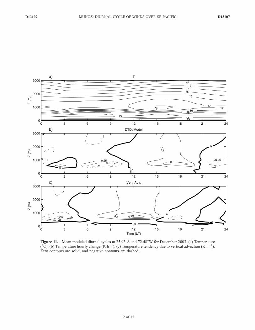
Figure 11. Mean modeled diurnal cycles at 25.93�S and 72.48�W for December 2003. (a) Temperature(�C). (b) Temperature hourly change (K h�1). (c) Temperature tendency due to vertical advection (K h�1).Zero contours are solid, and negative contours are dashed.


12 of 15

D13107

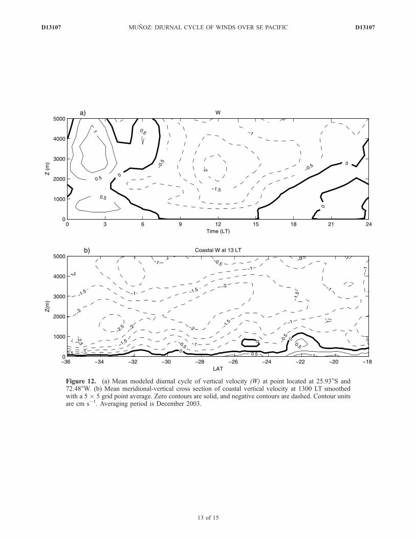
Figure 12. (a) Mean modeled diurnal cycle of vertical velocity (W) at point located at 25.93�S and72.48�W. (b) Mean meridional-vertical cross section of coastal vertical velocity at 1300 LT smoothedwith a 5 � 5 grid point average. Zero contours are solid, and negative contours are dashed. Contour unitsare cm s�1. Averaging period is December 2003.


13 of 15

D13107

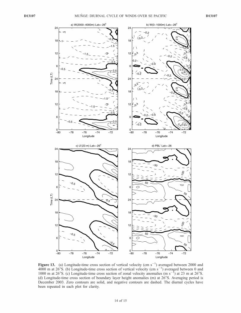
Figure 13. (a) Longitude-time cross section of vertical velocity (cm s�1) averaged between 2000 and4000 m at 26�S. (b) Longitude-time cross section of vertical velocity (cm s�1) averaged between 0 and1000 m at 26�S. (c) Longitude-time cross section of zonal velocity anomalies (m s�1) at 23 m at 26�S.(d) Longitude-time cross section of boundary layer height anomalies (m) at 26�S. Averaging period isDecember 2003. Zero contours are solid, and negative contours are dashed. The diurnal cycles havebeen repeated in each plot for clarity.


14 of 15

D13107

MBL response add constructively is where the largestsurface wind diurnal cycles are to be found.[31] The exact nature of the interaction of the low-

tropospheric flow with the Andes topography that producesthe nocturnal upsidence wave and the afternoon coastalenhanced subsidence has not been addressed in this work.Sensitivity model runs with changes in the Andes topographycould be used in the future to shed some light on this problem.Meanwhile the results herein stress the importance of ade-quate monitoring and modeling of the conditions in the lowtroposphere above the MBL if one is to reproduce appropri-ately the dynamics of theMBL in this region. This conclusionis particularly relevant in view of the upcoming Variability ofthe American Monsoon Systems (VAMOS) Ocean-Cloud-Atmosphere-Land Study Regional Experiment (VOCALS-REx) to be carried out by the end of 2008, aimed at betterunderstanding and modeling the dynamics of this importantstratocumulus capped MBL (R. Wood et al., 2006,VOCALS-SouthEast Pacific Regional Experiment (REx)Scientific Program Overview, available at http://www.eol.ucar.edu/projects/vocals/science_planning/VOCALS_SPO_rev_aug06.pdf).

[32] Acknowledgments. The author thanks R. Garreaud, J. Rutllant,B. Barrett, and two anonymous reviewers for numerous suggestions thatimproved the paper. This research was supported by CONICYT (Chile)under grants ACT-19 and Fondef D05I10038. QuikSCAT and SeaWindsdata are produced by Remote Sensing Systems and sponsored by theNASA Ocean Vector Winds Science Team. AMSR-E data are producedby Remote Sensing Systems and sponsored by the NASA Earth ScienceREASoN DISCOVER Project and the AMSR-E Science team. Data areavailable at www.remss.com.

ReferencesDai, A., and C. Deser (1999), Diurnal and semidiurnal variations inglobal surface wind and diveregence fields, J. Geophys. Res., 104,31,109–31,125.

Garreaud, R. D., and R. C. Munoz (2004), The diurnal cycle in circulationand cloudiness over the subtropical southeast Pacific: A modeling study,J. Clim., 17, 1699–1710.

Garreaud, R. D., and R. C. Munoz (2005), The low-level jet off the westcoast of subtropical South America: Structure and variability, Mon.Weather Rev., 133, 2246–2261.

Gayno, G. A. (1994), Development of a high-order, fog-producingboundary layer model suitable for use in numerical weather prediction,Master’s thesis, Pa. State Univ., University Park.

Gille, S. T., S. G. Llewellyn Smith, and S. M. Lee (2003), Measuring thesea breeze from QuikSCAT scatterometry, Geophys. Res. Lett., 30(3),1114, doi:10.1029/2002GL016230.

Gille, S. T., S. G. Llewellyn Smith, and N. M. Statom (2005), Globalobservations of the land breeze, Geophys. Res. Lett., 32, L05605,doi:10.1029/2004GL022139.

Grell, G. A., J. Dudhia, and D. R. Stauffer (1994), A description of the fifth-generation Penn State/NCAR mesoscale model (MM5), Tech. NoteNCAR/TN-398 + STR, Natl. Cent. for Atmos. Res., Boulder, Colo.

Hartmann, D. L., M. E. Ockert-Bell, and M. L. Michelsen (1992), Theeffect of cloud type on Earth’s energy balance: Global analysis, J. Clim.,5, 1281–1304.

Koracin, D., and C. E. Dorman (2001), Marine atmospheric boundary layerdivergence and clouds along California in June 1996, Mon. Weather Rev.,129, 2040–2056.

Lerczak, J. A., M. C. Hendershott, and C. D. Winant (2001), Observationsand modeling of coastal internal waves driven by a diurnal sea breeze,J. Geophys. Res., 106, 19,715–19,729.

McNoldy, B. D., P. E. Ciesielski, W. H. Shubert, and R. H. Johnson (2004),Surface winds, divergence, and vorticity in stratocumulus regions usingQuikSCAT and reanalysis winds, Geophys. Res. Lett., 31, L08105,doi:10.1029/2004GL019768.

Munoz, R. C., and R. D. Garreaud (2005), Dynamics of the low-level jet offthe west coast of subtropical South America, Mon. Weather Rev., 133,3661–3677.

Munoz, R. C., J. A. Rutllant, and R. D. Garreaud (2006), The diurnal cyclein the coastal atmospheric boundary layer along north central Chile:Observations and models, paper presented at the 8th International Con-ference on Southern Hemisphere Meteorology and Oceanography, Am.Meteorol. Soc., Foz do Iguazu, Brazil, 24–28 April.

Rozendaal, M. A., C. B. Leovy, and S. A. Klein (1995), An observationalstudy of diurnal variations of the marine stratiform clouds, J. Clim., 8,1795–1809.

Rutllant, J. A., H. Fuenzalida, and P. Aceituno (2003), Climate dynamicsalong the arid northern coast of Chile: The 1997–1998 Dinamica delClima de la Region de Antofagasta (DICLIMA) experiment, J. Geophys.Res., 108(D17), 4538, doi:10.1029/2002JD003357.

Rutllant, J. A., I. Masotti, J. Calderon, and S. A. Vega (2004), A compar-ison of spring coastal upwelling off central Chile at the extremes of the1996–1997 ENSO cycle, Cont. Shelf Res., 24, 773–787.

Shafran, P. C., N. L. Seaman, and G. A. Gayno (2000), Evaluation ofnumerical predictions of boundary layer structure during the Lake Michi-gan Ozone Study (LMOS), J. Appl. Meteorol., 39, 412–426.

Simpson, J. E. (1994), Sea Breeze and Local Winds, 234 pp., CambridgeUniv. Press, New York.

��R. C. Munoz, Department of Geophysics, University of Chile, Blanco

Encalada 2002, Santiago, Chile. ([email protected])


15 of 15

D13107

diurnal cycle of surface winds over the subtropical

Documents