diversified social media retrieval for news stories
TRANSCRIPT

Diversified Social Media Retrieval for News Stories.
Bryan Hang ZHANG
Feb. 25th 2016Master Thesis Colloquium
Department of Computational Linguistics
Dr. Vinay SETTY Prof. Dr. Günter NEUMANN
Supervisors:

Outline
• Motivation
• Related Work
• Solution
• Experiment Evaluation
• Conclusion
• Acknowledgement

Motivation
• Social media data is generated by users constantly.
• Blogs
• Forums (Quora, WEBMD….)
• Comments (Reddit, Instagram, YouTube….)

Motivation
query: news story
Thread
Thread
Rank: 2nd
Rank: 3rd
ThreadRank: 1st
Rank: K th Thread
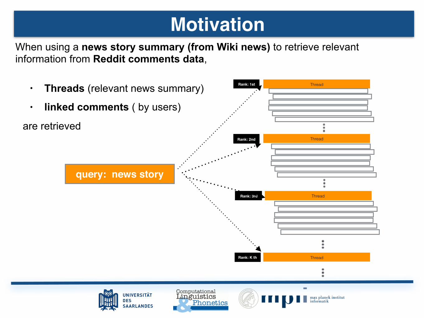
When using a news story summary (from Wiki news) to retrieve relevant information from Reddit comments data,
• Threads (relevant news summary)
•
are retrieved
Motivation
query: news story
Thread
Thread
Rank: 2nd
Rank: 3rd
ThreadRank: 1st
Rank: K th Thread
When using a news story summary (from Wiki news) to retrieve relevant information from Reddit comments data,
• Threads (relevant news summary)
• linked comments ( by users)
are retrieved

Motivation
query: news story
Thread
Thread
Rank: 2nd
Rank: 3rd
ThreadRank: 1st
Rank: K th Thread
When using a news story summary (from Wiki news) to retrieve relevant information from Reddit comments data,
• Threads (relevant news summary)
• linked comments ( by users)
are retrieved
Tree

Motivation
Tree-Structured Comments

Motivation
query: news story
Cuba Wants Off U.S. Terrorism List Before Restoring Normal Ties
Most Americans Support Renewed U.S.-Cuba Relations
Obama announces historic overhaul of relations; Cuba releases American
Raul Castro: US Must Return Guantanamo for Normal Relations
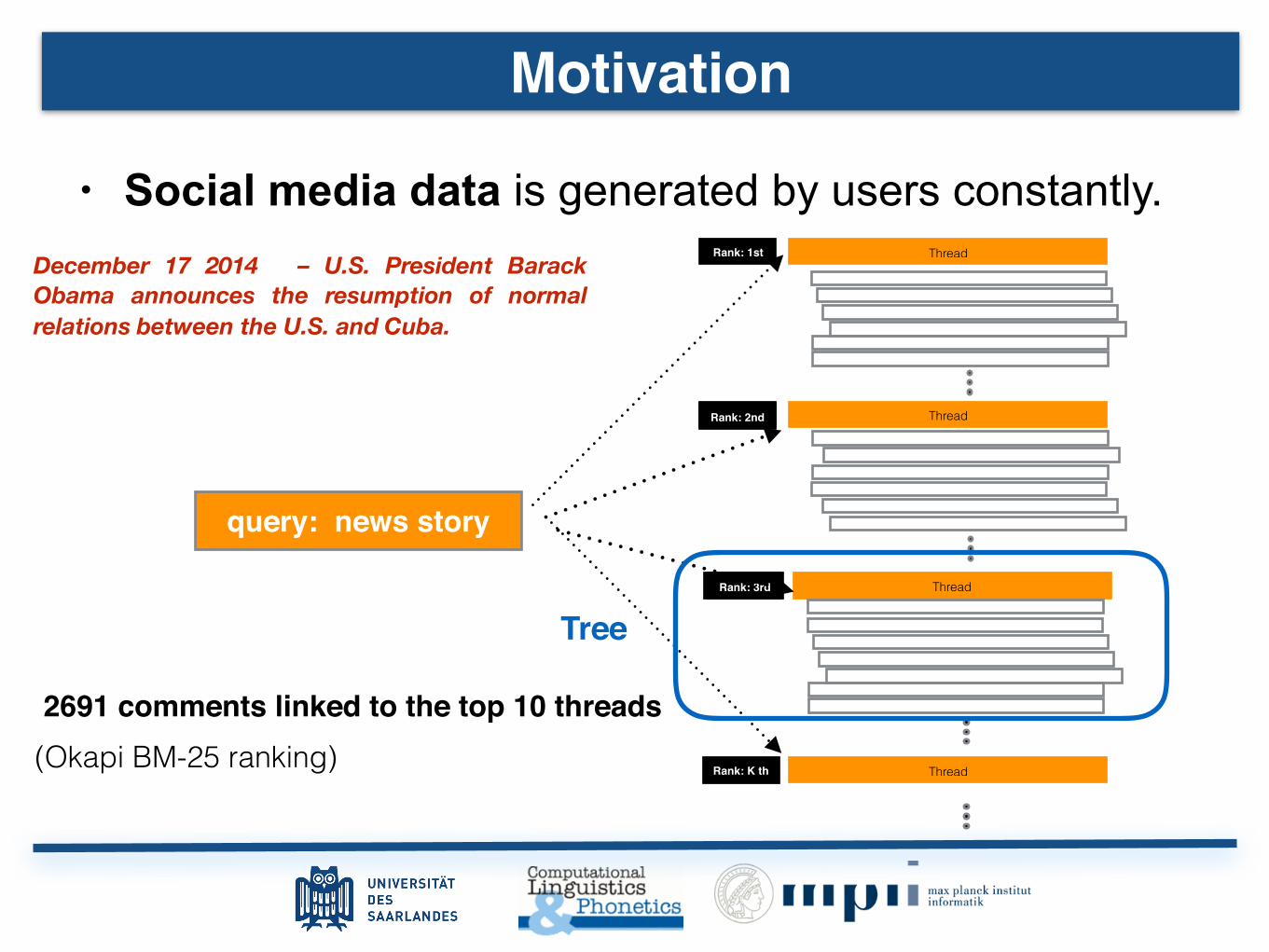
• Social media data is generated by users constantly. December 17 2014 – U.S. President Barack Obama announces the resumption of normal relations between the U.S. and Cuba.
2691 comments linked to the top 10 threads
(Okapi BM-25 ranking)
Motivation
query: news story
Thread
Thread
Rank: 2nd
Rank: 3rd
ThreadRank: 1st
Rank: K th Thread
• Social media data is generated by users constantly. December 17 2014 – U.S. President Barack Obama announces the resumption of normal relations between the U.S. and Cuba.
2691 comments linked to the top 10 threads (Okapi BM-25 ranking)
Tree

Motivation
News storypseudo search
result (thread+ linked
comment)
diversified search result
(concise, diverse result list)
Data: Reddit data Subreddit(category): Politics / World News
• The goal is to reduce the Redundancy in the pseudo search result from Reddit comments for news stories and create a concise and diversified search result.

Related Work• Research focusing on the reflection of ambiguity of a query in
the retrieved results and reduce redundancy: Implicit diversification methods: reduce redundancy based on documents content dissimilarity • Maximum Marginal Relevance [4] • BIR[6]
Explicit diversification methods: explicitly models the aspects (topics, categories) of a query and consider which query aspects individual documents relate to.•IA-Diversity[1] (user intention) •xQuad[2] (query reformation) •PM[3,5] (proportional representation covering the query
aspects)
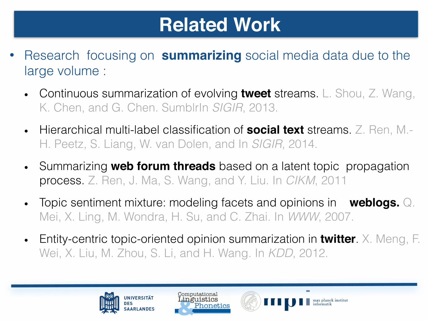
Related Work• Research focusing on summarizing social media data due to the
large volume : • Continuous summarization of evolving tweet streams. L. Shou, Z. Wang,
K. Chen, and G. Chen. SumblrIn SIGIR, 2013.
• Hierarchical multi-label classification of social text streams. Z. Ren, M.-H. Peetz, S. Liang, W. van Dolen, and In SIGIR, 2014.
• Summarizing web forum threads based on a latent topic propagation process. Z. Ren, J. Ma, S. Wang, and Y. Liu. In CIKM, 2011
• Topic sentiment mixture: modeling facets and opinions in weblogs. Q. Mei, X. Ling, M. Wondra, H. Su, and C. Zhai. In WWW, 2007.
• Entity-centric topic-oriented opinion summarization in twitter. X. Meng, F. Wei, X. Liu, M. Zhou, S. Li, and H. Wang. In KDD, 2012.

Related Work
There is no retrieval diversification work that has been done on the unedited, coherent, short, Tree-Structured comments

Solution Overview
comments retrieval
text pre- processing
topic modelling diversification

Solution Overview
elastic search system
text pre-processing
topic modelling diversification
• Top k threads
Text-based scoring using Okapi BM-25
(linked comments)

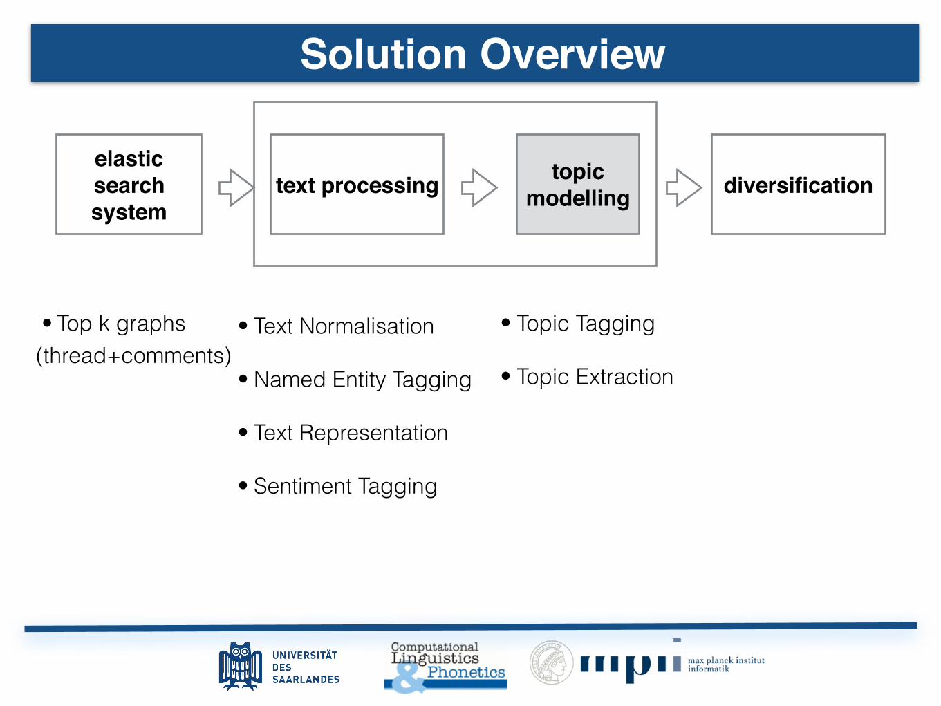
Solution Overview
elastic search system
text processing topic modelling diversification
• Top k threads • Text Normalisation
• Named Entity Tagging
• Text Representation (for better topical clustering)
• Sentiment Tagging
(linked comments)

Text Pre-processing • Remove urls (using Twokenizer) and non-alphanumeric symbols, sentence
tokenisation (NLTK sentence tokenizer)
• Sentiment Analysis VADER (rule-besed sentiment tagger)
• Part-of-Speech/ Named Entity Tagging Senna Tagger (Neural Network architecture - based tagger)
1. Duplicate Named Entities because there are more entity-based topic type in social media.
2. Select words according to the Penn Treebank part-of-speech tags. (according to Centering Theory)
3. Lemmatise selected words (NLTK Lemmatiser)

Text Pre-processing

Text Pre-processing
“The original article i read a couple months ago was in Der Spiegel and said nothing of a new or alternative party, although its possible i forgot.”
['DER_SPIEGEL', 'DER_SPIEGEL', 'original', 'article', 'read', 'couple', 'month', 'ago', 'der', 'spiegel', 'said', 'nothing', 'new', 'alternative', 'party', 'possible', 'forgot', 'here', 'related', 'article']
"The *Titanic* has hit an iceberg - and takes on more passengers …P.S. Yeah, keep those downvotes coming: they won't change reality, e.g. the unemployment figures in the Eurozone."
[TITANIC’, 'TITANIC', 'EUROZONE', 'EUROZONE', 'titanic', 'ha', 'hit', 'iceberg', 'take', 'on', 'more', 'passenger', 'keep', 'downvotes', 'coming', 'won', 'change', 'reality', 'figure', ‘eurozone']
Named Entity Named Entity word word word
Solution Overview
elastic search system
text processing topic modelling diversification
• Top k graphs • Topic Tagging
• Topic Extraction
• Text Normalisation
• Named Entity Tagging
• Text Representation
• Sentiment Tagging
(thread+comments)

Clustering • There are many clustering and topical modelling techniques:
k-means, hierarchical clustering, frequent set clustering, LDA, pLSA.
• Challenges for modelling topics for reddit comments.
• Comments are short. k-means, hierarchical clustering, LDA
• Unpredicted number of topics. LDA, pLSA
• Topical clusters interpretation. LDA
• Ungrammatical sentences and sentence fragments.
Relations from Collapsed Typed Dependencies cannot be accurately extracted.
Topic Modelling

Clustering
the sum of the total probability over all mixture components:
P (d) =KX
k=1
P (d|z = k)P (z = k) (6)
K is the number of mixture components (clusters). It[41] has the assumptions:
• The words in a document are generated independently when the document”s cluster
label k is known
• The probability of a word is independent of its position within the document.
It [41] assumes that each mixture component(cluster) is a multinomial distribution over
words and a Dirichlet distribution is also assumed as the prior for each mixture component
(cluster):
P (w|z = k) = P (w|z = k,�) = �k,w whereVX
w
�w,k = 1 and P (�|~�) = Dir(~✓|~�)
They also assume that the weight of each mixture component (cluster) is sampled from
a multinomial distribution and a Dirichlet prior for this multinomial distribution is also
assumed:
P (z = k) = P (z = k|⇥) = ✓k whereKX
k
✓k = 1 and P (⇥|~↵) = Dir(~✓|~↵)
collapsed Gibbs Samplings for GSDMM is introduced in [59], documents are randomly
assigned to K clusters initially and the following information is recorded: the cluster
labels of each document ~z, mz is number of documents in each cluster z , and n
wz is the
number of occurrences of word w in each cluster z, then documents are traversed for a
number of iterations. In each iteration, each document is reassigned to a cluster according
to the conditional distribution of P (Zd = z|~z¬d)the cluster z given the document ~
d and
cluster ~z¬d:
P (Zd = z|~z¬d) / mz,¬d + ↵
D � 1 +K↵
Qw2d
NwdQ
j=1(nw
z,¬d + � + j � 1)
NdQi=1
(nz,¬d + V � + i� 1)
Hyperparameter ↵ controls the popularity of the clusters. When ↵ gets larger, a document
has a larger probability to be assigned to an empty cluster; when ↵ = 0, a cluster will
be discarded after it gets empty. Therefore, the number of non-empty clusters found by
GSDMM gets larger slightly with the increase of ↵. Hyperparameter � emphasizes on the
14
1.select a mixture component(cluster) k
2. The selected mixture component(cluster) k generates d
Figure 1: Graphical model of DMM.
V number of words in the vocabularyD number of documents in the corpusL average length of documentsd documents in the corpusz cluster labels of each documentI number of iterationsmz number of documents in cluster z
nz number of words in cluster z
nwz number of occurrences of word w in cluster z
Nd number of words in document d
Nwd number of occurrences of word w in document d
Table 1: Notations
probability over all mixture components:
p(d) =K!
k=1
p(d|z = k)p(z = k) (1)
Here, K is the number of mixture components (clusters).Now, the problem becomes how to define p(d|z = k) andp(z = k). DMM makes the Naive Bayes assumption: thatthe words in a document are generated independently whenthe document’s cluster label k is known, and the probabilityof a word is independent of its position within the document.Then the probability of document d generated by cluster kcan be derived as follows:
p(d|z = k) ="
w∈d
p(w|z = k) (2)
Nigam et al. [20] assumes that each mixture component(cluster) is a multinomial distribution over words, such thatp(w|z = k) = p(w|z = k,Φ) = φk,w, where w = 1, ..., Vand
#w φk,w = 1. They assume a Dirichlet distribution as
the prior for each mixture component (cluster), such that
p(Φ|β) = Dir(φk|β). They also assume that the weight ofeach mixture component (cluster) is sampled from a multi-nomial distribution, such that p(z = k) = p(z = k|Θ) = θk,where k = 1, ..., K and
#k θk = 1. In addition, they assume
a Dirichlet prior for this multinomial distribution, such thatp(Θ|α) = Dir(θ|α).
The graphical model of DMM is shown in Figure 1. Inour short text clustering problem, we need to estimate themixture component (cluster) z for each document d. Wewill introduce our GSDMM algorithm with the help of theMovie Group Process (MGP) in the next section.
2.3 Gibbs Sampling for DMMIn this section, we introduce the collapsed Gibbs Sampling
algorithm for the Dirichlet Multinomial Mixture model (ab-br. to GSDMM), which is equivalent to the Movie GroupProcess (MGP) introduced in Section 2.1.
The detail of our GSDMM algorithm is shown in Algo-rithm 1, and the meaning of its variables is shown in Table1. In the initialization step, we randomly assign the docu-
ments to K clusters, and record the following information:z (cluster labels of each document), mz (number of docu-ments in cluster z), nz (number of words in cluster z), andnwz (number of occurrences of word w in cluster z). Then
we traverse the documents for I iterations. (In Section 4.4,we found that GSDMM can achieve good and stable perfor-mance when I equals five.) In each iteration, we re-assigna cluster for each document d in turn according to the con-ditional distribution: p(zd = z|z¬d, d), where ¬d means thecluster label of document d is removed from z. Each timewe re-assign a cluster z to document d, the correspondinginformation in z, mz, nz, and nw
z are updated accordingly.Finally, only a part of the initial K clusters will remain non-empty, in other words, GSDMM can cluster the documentsinto several groups. Through experimental study in Section4.5, we found that the number of non-empty clusters foundby GSDMM can be near the true number of groups as longas K is larger than the true number. GSDMM is also a softclustering model like Gaussian Mixture Model (GMM) [5],since we can get the probability of each document belongingto each cluster from p(zd = z|z¬d, d).
Algorithm 1: GSDMM
Data: Documents in the input, d.Result: Cluster labels of each document, z.begin
initialize mz, nz, and nwz as zero for each cluster z
for each document d ∈ [1, D] dosample a cluster for d:zd ← z ∼Multinomial(1/K)mz ← mz + 1 and nz ← nz +Nd
for each word w ∈ d donwz ← nw
z +Nwd
for i ∈ [1, I ] dofor each document d ∈ [1, D] do
record the current cluster of d: z = zdmz ← mz − 1 and nz ← nz −Nd
for each word w ∈ d donwz ← nw
z −Nwd
sample a cluster for d:zd ← z ∼ p(zd = z|z¬d, d) (Equation 4)mz ← mz + 1 and nz ← nz +Nd
for each word w ∈ d donwz ← nw
z +Nwd
We can derive p(zd = z|z¬d, d) from the Dirichlet Multi-nomial Mixture (DMM) model, and find that it conformsto the two rules of MGP introduced in Section 2.1. Wejust introduce the results directly here, and will explain thederivation details in the next section.
If we assume each word can at most appear once in eachdocument (In the movie group example, the assumption isthat a movie can at most appear once in each student’slist). We can derive a quite elegant form of the conditionaldistribution as follows:
p(zd = z|z¬d, d) ∝
mz,¬d + αD − 1 +Kα
$w∈d(n
wz,¬d + β)
$Ndi=1(nz,¬d + V β + i− 1)
(3)
235
the sum of the total probability over all mixture components:
P (d) =KX
k=1
P (d|z = k)P (z = k) (6)
K is the number of mixture components (clusters). It[41] has the assumptions:
• The words in a document are generated independently when the document”s cluster
label k is known
• The probability of a word is independent of its position within the document.
It [41] assumes that each mixture component(cluster) is a multinomial distribution over
words and a Dirichlet distribution is also assumed as the prior for each mixture component
(cluster):
P (w|z = k) = P (w|z = k,�) = �k,w whereVX
w
�w,k = 1 and P (�|~�) = Dir(~✓|~�)
They also assume that the weight of each mixture component (cluster) is sampled from
a multinomial distribution and a Dirichlet prior for this multinomial distribution is also
assumed:
P (z = k) = P (z = k|⇥) = ✓k whereKX
k
✓k = 1 and P (⇥|~↵) = Dir(~✓|~↵)
collapsed Gibbs Samplings for GSDMM is introduced in [59], documents are randomly
assigned to K clusters initially and the following information is recorded: the cluster
labels of each document ~z, mz is number of documents in each cluster z , and n
wz is the
number of occurrences of word w in each cluster z, then documents are traversed for a
number of iterations. In each iteration, each document is reassigned to a cluster according
to the conditional distribution of P (Zd = z|~z¬d)the cluster z given the document ~
d and
cluster ~z¬d:
P (Zd = z|~z¬d) / mz,¬d + ↵
D � 1 +K↵
Qw2d
NwdQ
j=1(nw
z,¬d + � + j � 1)
NdQi=1
(nz,¬d + V � + i� 1)
Hyperparameter ↵ controls the popularity of the clusters. When ↵ gets larger, a document
has a larger probability to be assigned to an empty cluster; when ↵ = 0, a cluster will
be discarded after it gets empty. Therefore, the number of non-empty clusters found by
GSDMM gets larger slightly with the increase of ↵. Hyperparameter � emphasizes on the
14
Dirichlet Multinomial Mixture Model (DMM)
Topic Modeling Topic Modelling
d
Your Paper
You
February 29, 2016
Abstract
Your abstract.
1 Introduction
↵⇥��
2 Some LATEX Examples
2.1 How to Leave Comments
Comments can be added to the margins of the document using the todo com- Here’s acommentin themargin!
Here’s acommentin themargin!
mand, as shown in the example on the right. You can also add inline comments:
This is an inline comment.
2.2 How to Include Figures
First you have to upload the image file (JPEG, PNG or PDF) from your com-puter to writeLaTeX using the upload link the project menu. Then use theincludegraphics command to include it in your document. Use the figure en-vironment and the caption command to add a number and a caption to yourfigure. See the code for Figure 1 in this section for an example.
2.3 How to Make Tables
Use the table and tabular commands for basic tables — see Table 1, for example.
Item QuantityWidgets 42Gadgets 13
Table 1: An example table.
1
Your Paper
You
February 29, 2016
Abstract
Your abstract.
1 Introduction
zdDK↵⇥��
2 Some LATEX Examples
2.1 How to Leave Comments
Comments can be added to the margins of the document using the todo com- Here’s acommentin themargin!
Here’s acommentin themargin!
mand, as shown in the example on the right. You can also add inline comments:
This is an inline comment.
2.2 How to Include Figures
First you have to upload the image file (JPEG, PNG or PDF) from your com-puter to writeLaTeX using the upload link the project menu. Then use theincludegraphics command to include it in your document. Use the figure en-vironment and the caption command to add a number and a caption to yourfigure. See the code for Figure 1 in this section for an example.
2.3 How to Make Tables
Use the table and tabular commands for basic tables — see Table 1, for example.
1

Clustering Dirichlet Multinomial Mixture Model (DMM)
Figure 1: Graphical model of DMM.
V number of words in the vocabularyD number of documents in the corpusL average length of documentsd documents in the corpusz cluster labels of each documentI number of iterationsmz number of documents in cluster z
nz number of words in cluster z
nwz number of occurrences of word w in cluster z
Nd number of words in document d
Nwd number of occurrences of word w in document d
Table 1: Notations
probability over all mixture components:
p(d) =K!
k=1
p(d|z = k)p(z = k) (1)
Here, K is the number of mixture components (clusters).Now, the problem becomes how to define p(d|z = k) andp(z = k). DMM makes the Naive Bayes assumption: thatthe words in a document are generated independently whenthe document’s cluster label k is known, and the probabilityof a word is independent of its position within the document.Then the probability of document d generated by cluster kcan be derived as follows:
p(d|z = k) ="
w∈d
p(w|z = k) (2)
Nigam et al. [20] assumes that each mixture component(cluster) is a multinomial distribution over words, such thatp(w|z = k) = p(w|z = k,Φ) = φk,w, where w = 1, ..., Vand
#w φk,w = 1. They assume a Dirichlet distribution as
the prior for each mixture component (cluster), such that
p(Φ|β) = Dir(φk|β). They also assume that the weight ofeach mixture component (cluster) is sampled from a multi-nomial distribution, such that p(z = k) = p(z = k|Θ) = θk,where k = 1, ..., K and
#k θk = 1. In addition, they assume
a Dirichlet prior for this multinomial distribution, such thatp(Θ|α) = Dir(θ|α).
The graphical model of DMM is shown in Figure 1. Inour short text clustering problem, we need to estimate themixture component (cluster) z for each document d. Wewill introduce our GSDMM algorithm with the help of theMovie Group Process (MGP) in the next section.
2.3 Gibbs Sampling for DMMIn this section, we introduce the collapsed Gibbs Sampling
algorithm for the Dirichlet Multinomial Mixture model (ab-br. to GSDMM), which is equivalent to the Movie GroupProcess (MGP) introduced in Section 2.1.
The detail of our GSDMM algorithm is shown in Algo-rithm 1, and the meaning of its variables is shown in Table1. In the initialization step, we randomly assign the docu-
ments to K clusters, and record the following information:z (cluster labels of each document), mz (number of docu-ments in cluster z), nz (number of words in cluster z), andnwz (number of occurrences of word w in cluster z). Then
we traverse the documents for I iterations. (In Section 4.4,we found that GSDMM can achieve good and stable perfor-mance when I equals five.) In each iteration, we re-assigna cluster for each document d in turn according to the con-ditional distribution: p(zd = z|z¬d, d), where ¬d means thecluster label of document d is removed from z. Each timewe re-assign a cluster z to document d, the correspondinginformation in z, mz, nz, and nw
z are updated accordingly.Finally, only a part of the initial K clusters will remain non-empty, in other words, GSDMM can cluster the documentsinto several groups. Through experimental study in Section4.5, we found that the number of non-empty clusters foundby GSDMM can be near the true number of groups as longas K is larger than the true number. GSDMM is also a softclustering model like Gaussian Mixture Model (GMM) [5],since we can get the probability of each document belongingto each cluster from p(zd = z|z¬d, d).
Algorithm 1: GSDMM
Data: Documents in the input, d.Result: Cluster labels of each document, z.begin
initialize mz, nz, and nwz as zero for each cluster z
for each document d ∈ [1, D] dosample a cluster for d:zd ← z ∼Multinomial(1/K)mz ← mz + 1 and nz ← nz +Nd
for each word w ∈ d donwz ← nw
z +Nwd
for i ∈ [1, I ] dofor each document d ∈ [1, D] do
record the current cluster of d: z = zdmz ← mz − 1 and nz ← nz −Nd
for each word w ∈ d donwz ← nw
z −Nwd
sample a cluster for d:zd ← z ∼ p(zd = z|z¬d, d) (Equation 4)mz ← mz + 1 and nz ← nz +Nd
for each word w ∈ d donwz ← nw
z +Nwd
We can derive p(zd = z|z¬d, d) from the Dirichlet Multi-nomial Mixture (DMM) model, and find that it conformsto the two rules of MGP introduced in Section 2.1. Wejust introduce the results directly here, and will explain thederivation details in the next section.
If we assume each word can at most appear once in eachdocument (In the movie group example, the assumption isthat a movie can at most appear once in each student’slist). We can derive a quite elegant form of the conditionaldistribution as follows:
p(zd = z|z¬d, d) ∝
mz,¬d + αD − 1 +Kα
$w∈d(n
wz,¬d + β)
$Ndi=1(nz,¬d + V β + i− 1)
(3)
235
the sum of the total probability over all mixture components:
P (d) =KX
k=1
P (d|z = k)P (z = k) (6)
K is the number of mixture components (clusters). It[41] has the assumptions:
• The words in a document are generated independently when the document”s cluster
label k is known
• The probability of a word is independent of its position within the document.
It [41] assumes that each mixture component(cluster) is a multinomial distribution over
words and a Dirichlet distribution is also assumed as the prior for each mixture component
(cluster):
P (w|z = k) = P (w|z = k,�) = �k,w whereVX
w
�w,k = 1 and P (�|~�) = Dir(~✓|~�)
They also assume that the weight of each mixture component (cluster) is sampled from
a multinomial distribution and a Dirichlet prior for this multinomial distribution is also
assumed:
P (z = k) = P (z = k|⇥) = ✓k whereKX
k
✓k = 1 and P (⇥|~↵) = Dir(~✓|~↵)
collapsed Gibbs Samplings for GSDMM is introduced in [59], documents are randomly
assigned to K clusters initially and the following information is recorded: the cluster
labels of each document ~z, mz is number of documents in each cluster z , and n
wz is the
number of occurrences of word w in each cluster z, then documents are traversed for a
number of iterations. In each iteration, each document is reassigned to a cluster according
to the conditional distribution of P (Zd = z|~z¬d)the cluster z given the document ~
d and
cluster ~z¬d:
P (Zd = z|~z¬d) / mz,¬d + ↵
D � 1 +K↵
Qw2d
NwdQ
j=1(nw
z,¬d + � + j � 1)
NdQi=1
(nz,¬d + V � + i� 1)
Hyperparameter ↵ controls the popularity of the clusters. When ↵ gets larger, a document
has a larger probability to be assigned to an empty cluster; when ↵ = 0, a cluster will
be discarded after it gets empty. Therefore, the number of non-empty clusters found by
GSDMM gets larger slightly with the increase of ↵. Hyperparameter � emphasizes on the
14
1. Select a mixture component(cluster) k
2. The selected mixture component(cluster) k generates d
Figure 1: Graphical model of DMM.
V number of words in the vocabularyD number of documents in the corpusL average length of documentsd documents in the corpusz cluster labels of each documentI number of iterationsmz number of documents in cluster z
nz number of words in cluster z
nwz number of occurrences of word w in cluster z
Nd number of words in document d
Nwd number of occurrences of word w in document d
Table 1: Notations
probability over all mixture components:
p(d) =K!
k=1
p(d|z = k)p(z = k) (1)
Here, K is the number of mixture components (clusters).Now, the problem becomes how to define p(d|z = k) andp(z = k). DMM makes the Naive Bayes assumption: thatthe words in a document are generated independently whenthe document’s cluster label k is known, and the probabilityof a word is independent of its position within the document.Then the probability of document d generated by cluster kcan be derived as follows:
p(d|z = k) ="
w∈d
p(w|z = k) (2)
Nigam et al. [20] assumes that each mixture component(cluster) is a multinomial distribution over words, such thatp(w|z = k) = p(w|z = k,Φ) = φk,w, where w = 1, ..., Vand
#w φk,w = 1. They assume a Dirichlet distribution as
the prior for each mixture component (cluster), such that
p(Φ|β) = Dir(φk|β). They also assume that the weight ofeach mixture component (cluster) is sampled from a multi-nomial distribution, such that p(z = k) = p(z = k|Θ) = θk,where k = 1, ..., K and
#k θk = 1. In addition, they assume
a Dirichlet prior for this multinomial distribution, such thatp(Θ|α) = Dir(θ|α).
The graphical model of DMM is shown in Figure 1. Inour short text clustering problem, we need to estimate themixture component (cluster) z for each document d. Wewill introduce our GSDMM algorithm with the help of theMovie Group Process (MGP) in the next section.
2.3 Gibbs Sampling for DMMIn this section, we introduce the collapsed Gibbs Sampling
algorithm for the Dirichlet Multinomial Mixture model (ab-br. to GSDMM), which is equivalent to the Movie GroupProcess (MGP) introduced in Section 2.1.
The detail of our GSDMM algorithm is shown in Algo-rithm 1, and the meaning of its variables is shown in Table1. In the initialization step, we randomly assign the docu-
ments to K clusters, and record the following information:z (cluster labels of each document), mz (number of docu-ments in cluster z), nz (number of words in cluster z), andnwz (number of occurrences of word w in cluster z). Then
we traverse the documents for I iterations. (In Section 4.4,we found that GSDMM can achieve good and stable perfor-mance when I equals five.) In each iteration, we re-assigna cluster for each document d in turn according to the con-ditional distribution: p(zd = z|z¬d, d), where ¬d means thecluster label of document d is removed from z. Each timewe re-assign a cluster z to document d, the correspondinginformation in z, mz, nz, and nw
z are updated accordingly.Finally, only a part of the initial K clusters will remain non-empty, in other words, GSDMM can cluster the documentsinto several groups. Through experimental study in Section4.5, we found that the number of non-empty clusters foundby GSDMM can be near the true number of groups as longas K is larger than the true number. GSDMM is also a softclustering model like Gaussian Mixture Model (GMM) [5],since we can get the probability of each document belongingto each cluster from p(zd = z|z¬d, d).
Algorithm 1: GSDMM
Data: Documents in the input, d.Result: Cluster labels of each document, z.begin
initialize mz, nz, and nwz as zero for each cluster z
for each document d ∈ [1, D] dosample a cluster for d:zd ← z ∼Multinomial(1/K)mz ← mz + 1 and nz ← nz +Nd
for each word w ∈ d donwz ← nw
z +Nwd
for i ∈ [1, I ] dofor each document d ∈ [1, D] do
record the current cluster of d: z = zdmz ← mz − 1 and nz ← nz −Nd
for each word w ∈ d donwz ← nw
z −Nwd
sample a cluster for d:zd ← z ∼ p(zd = z|z¬d, d) (Equation 4)mz ← mz + 1 and nz ← nz +Nd
for each word w ∈ d donwz ← nw
z +Nwd
We can derive p(zd = z|z¬d, d) from the Dirichlet Multi-nomial Mixture (DMM) model, and find that it conformsto the two rules of MGP introduced in Section 2.1. Wejust introduce the results directly here, and will explain thederivation details in the next section.
If we assume each word can at most appear once in eachdocument (In the movie group example, the assumption isthat a movie can at most appear once in each student’slist). We can derive a quite elegant form of the conditionaldistribution as follows:
p(zd = z|z¬d, d) ∝
mz,¬d + αD − 1 +Kα
$w∈d(n
wz,¬d + β)
$Ndi=1(nz,¬d + V β + i− 1)
(3)
235
the sum of the total probability over all mixture components:
P (d) =KX
k=1
P (d|z = k)P (z = k) (6)
K is the number of mixture components (clusters). It[41] has the assumptions:
• The words in a document are generated independently when the document”s cluster
label k is known
• The probability of a word is independent of its position within the document.
It [41] assumes that each mixture component(cluster) is a multinomial distribution over
words and a Dirichlet distribution is also assumed as the prior for each mixture component
(cluster):
P (w|z = k) = P (w|z = k,�) = �k,w whereVX
w
�w,k = 1 and P (�|~�) = Dir(~✓|~�)
They also assume that the weight of each mixture component (cluster) is sampled from
a multinomial distribution and a Dirichlet prior for this multinomial distribution is also
assumed:
P (z = k) = P (z = k|⇥) = ✓k whereKX
k
✓k = 1 and P (⇥|~↵) = Dir(~✓|~↵)
collapsed Gibbs Samplings for GSDMM is introduced in [59], documents are randomly
assigned to K clusters initially and the following information is recorded: the cluster
labels of each document ~z, mz is number of documents in each cluster z , and n
wz is the
number of occurrences of word w in each cluster z, then documents are traversed for a
number of iterations. In each iteration, each document is reassigned to a cluster according
to the conditional distribution of P (Zd = z|~z¬d)the cluster z given the document ~
d and
cluster ~z¬d:
P (Zd = z|~z¬d) / mz,¬d + ↵
D � 1 +K↵
Qw2d
NwdQ
j=1(nw
z,¬d + � + j � 1)
NdQi=1
(nz,¬d + V � + i� 1)
Hyperparameter ↵ controls the popularity of the clusters. When ↵ gets larger, a document
has a larger probability to be assigned to an empty cluster; when ↵ = 0, a cluster will
be discarded after it gets empty. Therefore, the number of non-empty clusters found by
GSDMM gets larger slightly with the increase of ↵. Hyperparameter � emphasizes on the
14
the sum of the total probability over all mixture components:
P (d) =KX
k=1
P (d|z = k)P (z = k) (6)
K is the number of mixture components (clusters). It[41] has the assumptions:
• The words in a document are generated independently when the document”s cluster
label k is known
• The probability of a word is independent of its position within the document.
It [41] assumes that each mixture component(cluster) is a multinomial distribution over
words and a Dirichlet distribution is also assumed as the prior for each mixture component
(cluster):
P (w|z = k) = P (w|z = k,�) = �k,w whereVX
w
�w,k = 1 and P (�|~�) = Dir(~✓|~�)
They also assume that the weight of each mixture component (cluster) is sampled from
a multinomial distribution and a Dirichlet prior for this multinomial distribution is also
assumed:
P (z = k) = P (z = k|⇥) = ✓k whereKX
k
✓k = 1 and P (⇥|~↵) = Dir(~✓|~↵)
collapsed Gibbs Samplings for GSDMM is introduced in [59], documents are randomly
assigned to K clusters initially and the following information is recorded: the cluster
labels of each document ~z, mz is number of documents in each cluster z , and n
wz is the
number of occurrences of word w in each cluster z, then documents are traversed for a
number of iterations. In each iteration, each document is reassigned to a cluster according
to the conditional distribution of P (Zd = z|~z¬d)the cluster z given the document ~
d and
cluster ~z¬d:
P (Zd = z|~z¬d) / mz,¬d + ↵
D � 1 +K↵
Qw2d
NwdQ
j=1(nw
z,¬d + � + j � 1)
NdQi=1
(nz,¬d + V � + i� 1)
Hyperparameter ↵ controls the popularity of the clusters. When ↵ gets larger, a document
has a larger probability to be assigned to an empty cluster; when ↵ = 0, a cluster will
be discarded after it gets empty. Therefore, the number of non-empty clusters found by
GSDMM gets larger slightly with the increase of ↵. Hyperparameter � emphasizes on the
14
Topic Modeling Topic Modelling

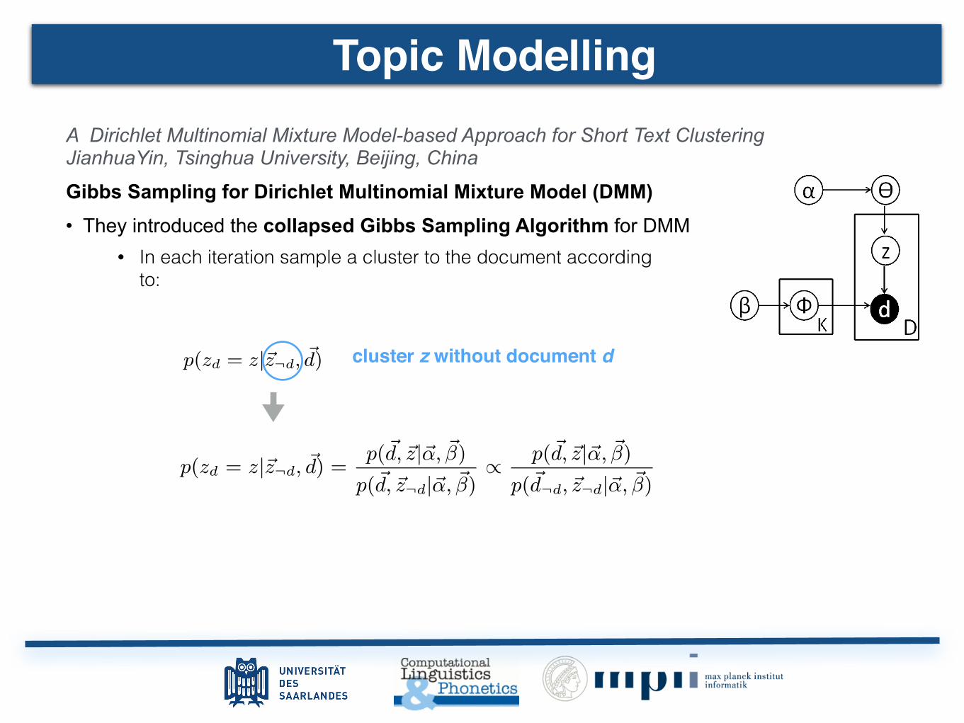
Topic Modeling A Dirichlet Multinomial Mixture Model-based Approach for Short Text Clustering JianhuaYin, Tsinghua University, Beijing, China
Gibbs Sampling for Dirichlet Multinomial Mixture Model (DMM) • They introduced the collapsed Gibbs Sampling Algorithm for DMM
Figure 1: Graphical model of DMM.
V number of words in the vocabularyD number of documents in the corpusL average length of documentsd documents in the corpusz cluster labels of each documentI number of iterationsmz number of documents in cluster z
nz number of words in cluster z
nwz number of occurrences of word w in cluster z
Nd number of words in document d
Nwd number of occurrences of word w in document d
Table 1: Notations
probability over all mixture components:
p(d) =K!
k=1
p(d|z = k)p(z = k) (1)
Here, K is the number of mixture components (clusters).Now, the problem becomes how to define p(d|z = k) andp(z = k). DMM makes the Naive Bayes assumption: thatthe words in a document are generated independently whenthe document’s cluster label k is known, and the probabilityof a word is independent of its position within the document.Then the probability of document d generated by cluster kcan be derived as follows:
p(d|z = k) ="
w∈d
p(w|z = k) (2)
Nigam et al. [20] assumes that each mixture component(cluster) is a multinomial distribution over words, such thatp(w|z = k) = p(w|z = k,Φ) = φk,w, where w = 1, ..., Vand
#w φk,w = 1. They assume a Dirichlet distribution as
the prior for each mixture component (cluster), such that
p(Φ|β) = Dir(φk|β). They also assume that the weight ofeach mixture component (cluster) is sampled from a multi-nomial distribution, such that p(z = k) = p(z = k|Θ) = θk,where k = 1, ..., K and
#k θk = 1. In addition, they assume
a Dirichlet prior for this multinomial distribution, such thatp(Θ|α) = Dir(θ|α).
The graphical model of DMM is shown in Figure 1. Inour short text clustering problem, we need to estimate themixture component (cluster) z for each document d. Wewill introduce our GSDMM algorithm with the help of theMovie Group Process (MGP) in the next section.
2.3 Gibbs Sampling for DMMIn this section, we introduce the collapsed Gibbs Sampling
algorithm for the Dirichlet Multinomial Mixture model (ab-br. to GSDMM), which is equivalent to the Movie GroupProcess (MGP) introduced in Section 2.1.
The detail of our GSDMM algorithm is shown in Algo-rithm 1, and the meaning of its variables is shown in Table1. In the initialization step, we randomly assign the docu-
ments to K clusters, and record the following information:z (cluster labels of each document), mz (number of docu-ments in cluster z), nz (number of words in cluster z), andnwz (number of occurrences of word w in cluster z). Then
we traverse the documents for I iterations. (In Section 4.4,we found that GSDMM can achieve good and stable perfor-mance when I equals five.) In each iteration, we re-assigna cluster for each document d in turn according to the con-ditional distribution: p(zd = z|z¬d, d), where ¬d means thecluster label of document d is removed from z. Each timewe re-assign a cluster z to document d, the correspondinginformation in z, mz, nz, and nw
z are updated accordingly.Finally, only a part of the initial K clusters will remain non-empty, in other words, GSDMM can cluster the documentsinto several groups. Through experimental study in Section4.5, we found that the number of non-empty clusters foundby GSDMM can be near the true number of groups as longas K is larger than the true number. GSDMM is also a softclustering model like Gaussian Mixture Model (GMM) [5],since we can get the probability of each document belongingto each cluster from p(zd = z|z¬d, d).
Algorithm 1: GSDMM
Data: Documents in the input, d.Result: Cluster labels of each document, z.begin
initialize mz, nz, and nwz as zero for each cluster z
for each document d ∈ [1, D] dosample a cluster for d:zd ← z ∼Multinomial(1/K)mz ← mz + 1 and nz ← nz +Nd
for each word w ∈ d donwz ← nw
z +Nwd
for i ∈ [1, I ] dofor each document d ∈ [1, D] do
record the current cluster of d: z = zdmz ← mz − 1 and nz ← nz −Nd
for each word w ∈ d donwz ← nw
z −Nwd
sample a cluster for d:zd ← z ∼ p(zd = z|z¬d, d) (Equation 4)mz ← mz + 1 and nz ← nz +Nd
for each word w ∈ d donwz ← nw
z +Nwd
We can derive p(zd = z|z¬d, d) from the Dirichlet Multi-nomial Mixture (DMM) model, and find that it conformsto the two rules of MGP introduced in Section 2.1. Wejust introduce the results directly here, and will explain thederivation details in the next section.
If we assume each word can at most appear once in eachdocument (In the movie group example, the assumption isthat a movie can at most appear once in each student’slist). We can derive a quite elegant form of the conditionaldistribution as follows:
p(zd = z|z¬d, d) ∝
mz,¬d + αD − 1 +Kα
$w∈d(n
wz,¬d + β)
$Ndi=1(nz,¬d + V β + i− 1)
(3)
235
• In each iteration sample a cluster to the document according to:
where Nd is the number of words in document d. In shorttext setting, Nd is often less than 100.
The first part of Equation 3 relates to Rule 1 of MG-P (Choose a table with more students). Here mz,¬d is thenumber of students (documents) in table z without consider-ing student d, and D is the total number of students. Whentable z has more students, the first part tends to be larger,and a student will tend to choose a table with more students.As a result, the first part of Equation 3 tends to result inlarge completeness, because it leads large tables (clusters)to be larger and students in the same ground true group aremore likely to be in the same table (cluster). The secondpart of Equation 3 relates to Rule 2 of MGP (Choose a ta-ble whose students share similar interests with him). Herenwz,¬d and nz,¬d are the number of occurrences of movie w
in table z and the total number of movies in table z with-out considering student d, respectively. When table z hasmore students sharing similar interests with student d (i.e.,watched more movies of the same), movies of student d willappear more often in table z (with larger nw
z,¬d), and theprobability of student d choosing table z will be larger. Asa result, the second part of Equation 3 tends to result inlarge homogeneity, because it can leads the students in thesame table to be more similar (more likely to be in the sameground true group).
If we allow a word to appear multi-times in a document(A movie can appear multi-times in a student’s list). Wecan derive the conditional probability as follows:
p(zd = z|z¬d, d) ∝
mz,¬d + αD − 1 +Kα
!w∈d
!Nwd
j=1(nwz,¬d + β + j − 1)
!Ndi=1(nz,¬d + V β + i− 1)
(4)
where Nwd is the number of occurrences of word w in doc-
ument d. We should note that the two parts of Equation 4have similar relationship with MGP like that of Equation 3,and the complexity of Equation 4 is the same as Equation 3.The only difference between them is the numerator of theirsecond part. We will try to derive Equation 3 and Equation4 from the Dirichlet Multinomial Mixture (DMM) model inthe next section.
2.4 Derivation of GSDMMIn this section, we try to formally derive the conditional
distribution p(zd = z|z¬d, d) used in our GSDMM algorithmas follows.
p(zd = z|z¬d, d) =p(d, z|α, β)
p(d, z¬d|α, β)∝
p(d, z|α, β)
p(d¬d, z¬d|α, β)(5)
where ¬d means document d is excluded from z and d. Nowwe need to derive the full distribution p(d, z|α, β). From the
graphical model of DMM in Figure 1, we can see p(d, z|α, β) =
p(d|z, β)p(z|α). Then we need to derive p(d|z, β) and p(z|α).Let us first investigate how to obtain p(z|α). We can see
that p(z|α) can be obtained by integrating with respect toΘ as p(z|α) =
"p(z|Θ)p(Θ|α)dΘ. As mentioned in Sec-
tion 2.2, p(Θ|α) is a Dirichlet distribution and p(z|Θ) isa multinomial distribution. With similar techniques of [9],
we can get p(z|α) = ∆(m+α)∆(α) , where m = {mk}
Kk=1, and
mk is the number of documents (students) in the kth clus-ter (table). Here we adopt the ∆ function in [9], and we
have ∆(α) =!K
k=1Γ(α)
Γ("
Kk=1
α)and ∆(m + α) =
!Kk=1
Γ(mk+α)
Γ("
Kk=1
(mk+α))=
!Kk=1
Γ(mk+α)Γ(D+Kα) , where D is the number of documents in the
dataset, D =#K
k=1 mk.
Similarly, p(d|z, β) can be obtained by integrating with re-
spect to Φ as p(d|z, β) ="p(d|z,Φ)p(Φ|β)dΦ =
!Kk=1
∆(nk+β)
∆(β),
where nk = {nwk }
Vw=1, and nw
k is the number of occurrences
of word w in the kth cluster (table). Similarly, ∆(β) =!V
w=1Γ(β)
Γ("
Vw=1
β)and∆(nk+β) =
!Vw=1
Γ(nwk +β)
Γ("
Vw=1
(nwk+β))
=!V
w=1Γ(nw
k +β)Γ(nk+V β) ,
where nk is number of words (movies) in document (table)k, that is, nk =
#Vw=1 n
wk .
Now the joint distribution becomes:
p(d, z|α, β) =∆(m+ α)
∆(α)
K$
k=1
∆(nk + β)
∆(β)
Then the conditional distribution in Equation 5 can be de-rived as follows:
p(zd = z|z¬d, d) ∝p(d, z|α, β)
p(d¬d, z¬d|α, β)
∝∆(m+ α)
∆(m¬d + α)∆(nz + β)
∆(nz,¬d + β)
∝Γ(mz + α)
Γ(mz,¬d + α)Γ(D − 1 +Kα)Γ(D +Kα)!
w∈d Γ(nwz + β)!
w∈d Γ(nwz,¬d + β)
Γ(nz,¬d + V β)Γ(nz + V β)
(6)
where mz = mz,¬d + 1 and nz = nz,¬d + Nd. Because Γ
function has the following property: Γ(x+m)Γ(x) =
!mi=1(x+ i−
1). We can rewrite Equation 6 into the following form:
p(zd = z|z¬d, d)
∝mz,¬d + αD − 1 +Kα
!w∈d Γ(nw
z +β)!
w∈d Γ(nwz,¬d
+β)!Nd
i=1(nz,¬d + V β + i− 1)(7)
When we assume each word can at most appear once ineach document (In the movie group example, the assumptionis a movie can at most appear once in each student’s list).
We can get!
w∈d Γ(nwz +β)
!w∈d Γ(nw
z,¬d+β) =
!w∈d(n
wz,¬d + β) since nw
z =
nwz,¬d +1 holds, and Equation 7 turns out to be Equation 3.When we allow a word to appear multi-times in each doc-
ument (A movie can appear multi-times in each student’s
list).We can get!
w∈d Γ(nwz +β)
!w∈d Γ(nw
z,¬d+β) =
!w∈d
!Nwd
j=1(nwz,¬d + β +
j − 1) since nwz = nw
z,¬d +Nwd holds, and Equation 7 turns
out to be Equation 4.
3. DISCUSSION
3.1 Meaning of Alpha and BetaIn this part, we try to explore the meaning of α and β with
the help of the Movie Group Process (MGP) as introducedin Section 2.1. From Equation 4, we can see that α relatesto the prior probability of a student (document) choosing atable (cluster). If we set α = 0, a table will never be chosenby the students once it gets empty, because the first part ofEquation 4 is now zero. When α gets larger, the probabilityof a student choosing an empty table will also gets larger.
236
Topic Modelling

Topic Modeling A Dirichlet Multinomial Mixture Model-based Approach for Short Text Clustering JianhuaYin, Tsinghua University, Beijing, China
Gibbs Sampling for Dirichlet Multinomial Mixture Model (DMM) • They introduced the collapsed Gibbs Sampling Algorithm for DMM
Figure 1: Graphical model of DMM.
V number of words in the vocabularyD number of documents in the corpusL average length of documentsd documents in the corpusz cluster labels of each documentI number of iterationsmz number of documents in cluster z
nz number of words in cluster z
nwz number of occurrences of word w in cluster z
Nd number of words in document d
Nwd number of occurrences of word w in document d
Table 1: Notations
probability over all mixture components:
p(d) =K!
k=1
p(d|z = k)p(z = k) (1)
Here, K is the number of mixture components (clusters).Now, the problem becomes how to define p(d|z = k) andp(z = k). DMM makes the Naive Bayes assumption: thatthe words in a document are generated independently whenthe document’s cluster label k is known, and the probabilityof a word is independent of its position within the document.Then the probability of document d generated by cluster kcan be derived as follows:
p(d|z = k) ="
w∈d
p(w|z = k) (2)
Nigam et al. [20] assumes that each mixture component(cluster) is a multinomial distribution over words, such thatp(w|z = k) = p(w|z = k,Φ) = φk,w, where w = 1, ..., Vand
#w φk,w = 1. They assume a Dirichlet distribution as
the prior for each mixture component (cluster), such that
p(Φ|β) = Dir(φk|β). They also assume that the weight ofeach mixture component (cluster) is sampled from a multi-nomial distribution, such that p(z = k) = p(z = k|Θ) = θk,where k = 1, ..., K and
#k θk = 1. In addition, they assume
a Dirichlet prior for this multinomial distribution, such thatp(Θ|α) = Dir(θ|α).
The graphical model of DMM is shown in Figure 1. Inour short text clustering problem, we need to estimate themixture component (cluster) z for each document d. Wewill introduce our GSDMM algorithm with the help of theMovie Group Process (MGP) in the next section.
2.3 Gibbs Sampling for DMMIn this section, we introduce the collapsed Gibbs Sampling
algorithm for the Dirichlet Multinomial Mixture model (ab-br. to GSDMM), which is equivalent to the Movie GroupProcess (MGP) introduced in Section 2.1.
The detail of our GSDMM algorithm is shown in Algo-rithm 1, and the meaning of its variables is shown in Table1. In the initialization step, we randomly assign the docu-
ments to K clusters, and record the following information:z (cluster labels of each document), mz (number of docu-ments in cluster z), nz (number of words in cluster z), andnwz (number of occurrences of word w in cluster z). Then
we traverse the documents for I iterations. (In Section 4.4,we found that GSDMM can achieve good and stable perfor-mance when I equals five.) In each iteration, we re-assigna cluster for each document d in turn according to the con-ditional distribution: p(zd = z|z¬d, d), where ¬d means thecluster label of document d is removed from z. Each timewe re-assign a cluster z to document d, the correspondinginformation in z, mz, nz, and nw
z are updated accordingly.Finally, only a part of the initial K clusters will remain non-empty, in other words, GSDMM can cluster the documentsinto several groups. Through experimental study in Section4.5, we found that the number of non-empty clusters foundby GSDMM can be near the true number of groups as longas K is larger than the true number. GSDMM is also a softclustering model like Gaussian Mixture Model (GMM) [5],since we can get the probability of each document belongingto each cluster from p(zd = z|z¬d, d).
Algorithm 1: GSDMM
Data: Documents in the input, d.Result: Cluster labels of each document, z.begin
initialize mz, nz, and nwz as zero for each cluster z
for each document d ∈ [1, D] dosample a cluster for d:zd ← z ∼Multinomial(1/K)mz ← mz + 1 and nz ← nz +Nd
for each word w ∈ d donwz ← nw
z +Nwd
for i ∈ [1, I ] dofor each document d ∈ [1, D] do
record the current cluster of d: z = zdmz ← mz − 1 and nz ← nz −Nd
for each word w ∈ d donwz ← nw
z −Nwd
sample a cluster for d:zd ← z ∼ p(zd = z|z¬d, d) (Equation 4)mz ← mz + 1 and nz ← nz +Nd
for each word w ∈ d donwz ← nw
z +Nwd
We can derive p(zd = z|z¬d, d) from the Dirichlet Multi-nomial Mixture (DMM) model, and find that it conformsto the two rules of MGP introduced in Section 2.1. Wejust introduce the results directly here, and will explain thederivation details in the next section.
If we assume each word can at most appear once in eachdocument (In the movie group example, the assumption isthat a movie can at most appear once in each student’slist). We can derive a quite elegant form of the conditionaldistribution as follows:
p(zd = z|z¬d, d) ∝
mz,¬d + αD − 1 +Kα
$w∈d(n
wz,¬d + β)
$Ndi=1(nz,¬d + V β + i− 1)
(3)
235
• In each iteration sample a cluster to the document according to:
where Nd is the number of words in document d. In shorttext setting, Nd is often less than 100.
The first part of Equation 3 relates to Rule 1 of MG-P (Choose a table with more students). Here mz,¬d is thenumber of students (documents) in table z without consider-ing student d, and D is the total number of students. Whentable z has more students, the first part tends to be larger,and a student will tend to choose a table with more students.As a result, the first part of Equation 3 tends to result inlarge completeness, because it leads large tables (clusters)to be larger and students in the same ground true group aremore likely to be in the same table (cluster). The secondpart of Equation 3 relates to Rule 2 of MGP (Choose a ta-ble whose students share similar interests with him). Herenwz,¬d and nz,¬d are the number of occurrences of movie w
in table z and the total number of movies in table z with-out considering student d, respectively. When table z hasmore students sharing similar interests with student d (i.e.,watched more movies of the same), movies of student d willappear more often in table z (with larger nw
z,¬d), and theprobability of student d choosing table z will be larger. Asa result, the second part of Equation 3 tends to result inlarge homogeneity, because it can leads the students in thesame table to be more similar (more likely to be in the sameground true group).
If we allow a word to appear multi-times in a document(A movie can appear multi-times in a student’s list). Wecan derive the conditional probability as follows:
p(zd = z|z¬d, d) ∝
mz,¬d + αD − 1 +Kα
!w∈d
!Nwd
j=1(nwz,¬d + β + j − 1)
!Ndi=1(nz,¬d + V β + i− 1)
(4)
where Nwd is the number of occurrences of word w in doc-
ument d. We should note that the two parts of Equation 4have similar relationship with MGP like that of Equation 3,and the complexity of Equation 4 is the same as Equation 3.The only difference between them is the numerator of theirsecond part. We will try to derive Equation 3 and Equation4 from the Dirichlet Multinomial Mixture (DMM) model inthe next section.
2.4 Derivation of GSDMMIn this section, we try to formally derive the conditional
distribution p(zd = z|z¬d, d) used in our GSDMM algorithmas follows.
p(zd = z|z¬d, d) =p(d, z|α, β)
p(d, z¬d|α, β)∝
p(d, z|α, β)
p(d¬d, z¬d|α, β)(5)
where ¬d means document d is excluded from z and d. Nowwe need to derive the full distribution p(d, z|α, β). From the
graphical model of DMM in Figure 1, we can see p(d, z|α, β) =
p(d|z, β)p(z|α). Then we need to derive p(d|z, β) and p(z|α).Let us first investigate how to obtain p(z|α). We can see
that p(z|α) can be obtained by integrating with respect toΘ as p(z|α) =
"p(z|Θ)p(Θ|α)dΘ. As mentioned in Sec-
tion 2.2, p(Θ|α) is a Dirichlet distribution and p(z|Θ) isa multinomial distribution. With similar techniques of [9],
we can get p(z|α) = ∆(m+α)∆(α) , where m = {mk}
Kk=1, and
mk is the number of documents (students) in the kth clus-ter (table). Here we adopt the ∆ function in [9], and we
have ∆(α) =!K
k=1Γ(α)
Γ("
Kk=1
α)and ∆(m + α) =
!Kk=1
Γ(mk+α)
Γ("
Kk=1
(mk+α))=
!Kk=1
Γ(mk+α)Γ(D+Kα) , where D is the number of documents in the
dataset, D =#K
k=1 mk.
Similarly, p(d|z, β) can be obtained by integrating with re-
spect to Φ as p(d|z, β) ="p(d|z,Φ)p(Φ|β)dΦ =
!Kk=1
∆(nk+β)
∆(β),
where nk = {nwk }
Vw=1, and nw
k is the number of occurrences
of word w in the kth cluster (table). Similarly, ∆(β) =!V
w=1Γ(β)
Γ("
Vw=1
β)and∆(nk+β) =
!Vw=1
Γ(nwk +β)
Γ("
Vw=1
(nwk+β))
=!V
w=1Γ(nw
k +β)Γ(nk+V β) ,
where nk is number of words (movies) in document (table)k, that is, nk =
#Vw=1 n
wk .
Now the joint distribution becomes:
p(d, z|α, β) =∆(m+ α)
∆(α)
K$
k=1
∆(nk + β)
∆(β)
Then the conditional distribution in Equation 5 can be de-rived as follows:
p(zd = z|z¬d, d) ∝p(d, z|α, β)
p(d¬d, z¬d|α, β)
∝∆(m+ α)
∆(m¬d + α)∆(nz + β)
∆(nz,¬d + β)
∝Γ(mz + α)
Γ(mz,¬d + α)Γ(D − 1 +Kα)Γ(D +Kα)!
w∈d Γ(nwz + β)!
w∈d Γ(nwz,¬d + β)
Γ(nz,¬d + V β)Γ(nz + V β)
(6)
where mz = mz,¬d + 1 and nz = nz,¬d + Nd. Because Γ
function has the following property: Γ(x+m)Γ(x) =
!mi=1(x+ i−
1). We can rewrite Equation 6 into the following form:
p(zd = z|z¬d, d)
∝mz,¬d + αD − 1 +Kα
!w∈d Γ(nw
z +β)!
w∈d Γ(nwz,¬d
+β)!Nd
i=1(nz,¬d + V β + i− 1)(7)
When we assume each word can at most appear once ineach document (In the movie group example, the assumptionis a movie can at most appear once in each student’s list).
We can get!
w∈d Γ(nwz +β)
!w∈d Γ(nw
z,¬d+β) =
!w∈d(n
wz,¬d + β) since nw
z =
nwz,¬d +1 holds, and Equation 7 turns out to be Equation 3.When we allow a word to appear multi-times in each doc-
ument (A movie can appear multi-times in each student’s
list).We can get!
w∈d Γ(nwz +β)
!w∈d Γ(nw
z,¬d+β) =
!w∈d
!Nwd
j=1(nwz,¬d + β +
j − 1) since nwz = nw
z,¬d +Nwd holds, and Equation 7 turns
out to be Equation 4.
3. DISCUSSION
3.1 Meaning of Alpha and BetaIn this part, we try to explore the meaning of α and β with
the help of the Movie Group Process (MGP) as introducedin Section 2.1. From Equation 4, we can see that α relatesto the prior probability of a student (document) choosing atable (cluster). If we set α = 0, a table will never be chosenby the students once it gets empty, because the first part ofEquation 4 is now zero. When α gets larger, the probabilityof a student choosing an empty table will also gets larger.
236
cluster z without document d
Topic Modelling
Topic Modeling A Dirichlet Multinomial Mixture Model-based Approach for Short Text Clustering JianhuaYin, Tsinghua University, Beijing, China
Gibbs Sampling for Dirichlet Multinomial Mixture Model (DMM) • They introduced the collapsed Gibbs Sampling Algorithm for DMM
Figure 1: Graphical model of DMM.
V number of words in the vocabularyD number of documents in the corpusL average length of documentsd documents in the corpusz cluster labels of each documentI number of iterationsmz number of documents in cluster z
nz number of words in cluster z
nwz number of occurrences of word w in cluster z
Nd number of words in document d
Nwd number of occurrences of word w in document d
Table 1: Notations
probability over all mixture components:
p(d) =K!
k=1
p(d|z = k)p(z = k) (1)
Here, K is the number of mixture components (clusters).Now, the problem becomes how to define p(d|z = k) andp(z = k). DMM makes the Naive Bayes assumption: thatthe words in a document are generated independently whenthe document’s cluster label k is known, and the probabilityof a word is independent of its position within the document.Then the probability of document d generated by cluster kcan be derived as follows:
p(d|z = k) ="
w∈d
p(w|z = k) (2)
Nigam et al. [20] assumes that each mixture component(cluster) is a multinomial distribution over words, such thatp(w|z = k) = p(w|z = k,Φ) = φk,w, where w = 1, ..., Vand
#w φk,w = 1. They assume a Dirichlet distribution as
the prior for each mixture component (cluster), such that
p(Φ|β) = Dir(φk|β). They also assume that the weight ofeach mixture component (cluster) is sampled from a multi-nomial distribution, such that p(z = k) = p(z = k|Θ) = θk,where k = 1, ..., K and
#k θk = 1. In addition, they assume
a Dirichlet prior for this multinomial distribution, such thatp(Θ|α) = Dir(θ|α).
The graphical model of DMM is shown in Figure 1. Inour short text clustering problem, we need to estimate themixture component (cluster) z for each document d. Wewill introduce our GSDMM algorithm with the help of theMovie Group Process (MGP) in the next section.
2.3 Gibbs Sampling for DMMIn this section, we introduce the collapsed Gibbs Sampling
algorithm for the Dirichlet Multinomial Mixture model (ab-br. to GSDMM), which is equivalent to the Movie GroupProcess (MGP) introduced in Section 2.1.
The detail of our GSDMM algorithm is shown in Algo-rithm 1, and the meaning of its variables is shown in Table1. In the initialization step, we randomly assign the docu-
ments to K clusters, and record the following information:z (cluster labels of each document), mz (number of docu-ments in cluster z), nz (number of words in cluster z), andnwz (number of occurrences of word w in cluster z). Then
we traverse the documents for I iterations. (In Section 4.4,we found that GSDMM can achieve good and stable perfor-mance when I equals five.) In each iteration, we re-assigna cluster for each document d in turn according to the con-ditional distribution: p(zd = z|z¬d, d), where ¬d means thecluster label of document d is removed from z. Each timewe re-assign a cluster z to document d, the correspondinginformation in z, mz, nz, and nw
z are updated accordingly.Finally, only a part of the initial K clusters will remain non-empty, in other words, GSDMM can cluster the documentsinto several groups. Through experimental study in Section4.5, we found that the number of non-empty clusters foundby GSDMM can be near the true number of groups as longas K is larger than the true number. GSDMM is also a softclustering model like Gaussian Mixture Model (GMM) [5],since we can get the probability of each document belongingto each cluster from p(zd = z|z¬d, d).
Algorithm 1: GSDMM
Data: Documents in the input, d.Result: Cluster labels of each document, z.begin
initialize mz, nz, and nwz as zero for each cluster z
for each document d ∈ [1, D] dosample a cluster for d:zd ← z ∼Multinomial(1/K)mz ← mz + 1 and nz ← nz +Nd
for each word w ∈ d donwz ← nw
z +Nwd
for i ∈ [1, I ] dofor each document d ∈ [1, D] do
record the current cluster of d: z = zdmz ← mz − 1 and nz ← nz −Nd
for each word w ∈ d donwz ← nw
z −Nwd
sample a cluster for d:zd ← z ∼ p(zd = z|z¬d, d) (Equation 4)mz ← mz + 1 and nz ← nz +Nd
for each word w ∈ d donwz ← nw
z +Nwd
We can derive p(zd = z|z¬d, d) from the Dirichlet Multi-nomial Mixture (DMM) model, and find that it conformsto the two rules of MGP introduced in Section 2.1. Wejust introduce the results directly here, and will explain thederivation details in the next section.
If we assume each word can at most appear once in eachdocument (In the movie group example, the assumption isthat a movie can at most appear once in each student’slist). We can derive a quite elegant form of the conditionaldistribution as follows:
p(zd = z|z¬d, d) ∝
mz,¬d + αD − 1 +Kα
$w∈d(n
wz,¬d + β)
$Ndi=1(nz,¬d + V β + i− 1)
(3)
235
• In each iteration sample a cluster to the document according to:
where Nd is the number of words in document d. In shorttext setting, Nd is often less than 100.
The first part of Equation 3 relates to Rule 1 of MG-P (Choose a table with more students). Here mz,¬d is thenumber of students (documents) in table z without consider-ing student d, and D is the total number of students. Whentable z has more students, the first part tends to be larger,and a student will tend to choose a table with more students.As a result, the first part of Equation 3 tends to result inlarge completeness, because it leads large tables (clusters)to be larger and students in the same ground true group aremore likely to be in the same table (cluster). The secondpart of Equation 3 relates to Rule 2 of MGP (Choose a ta-ble whose students share similar interests with him). Herenwz,¬d and nz,¬d are the number of occurrences of movie w
in table z and the total number of movies in table z with-out considering student d, respectively. When table z hasmore students sharing similar interests with student d (i.e.,watched more movies of the same), movies of student d willappear more often in table z (with larger nw
z,¬d), and theprobability of student d choosing table z will be larger. Asa result, the second part of Equation 3 tends to result inlarge homogeneity, because it can leads the students in thesame table to be more similar (more likely to be in the sameground true group).
If we allow a word to appear multi-times in a document(A movie can appear multi-times in a student’s list). Wecan derive the conditional probability as follows:
p(zd = z|z¬d, d) ∝
mz,¬d + αD − 1 +Kα
!w∈d
!Nwd
j=1(nwz,¬d + β + j − 1)
!Ndi=1(nz,¬d + V β + i− 1)
(4)
where Nwd is the number of occurrences of word w in doc-
ument d. We should note that the two parts of Equation 4have similar relationship with MGP like that of Equation 3,and the complexity of Equation 4 is the same as Equation 3.The only difference between them is the numerator of theirsecond part. We will try to derive Equation 3 and Equation4 from the Dirichlet Multinomial Mixture (DMM) model inthe next section.
2.4 Derivation of GSDMMIn this section, we try to formally derive the conditional
distribution p(zd = z|z¬d, d) used in our GSDMM algorithmas follows.
p(zd = z|z¬d, d) =p(d, z|α, β)
p(d, z¬d|α, β)∝
p(d, z|α, β)
p(d¬d, z¬d|α, β)(5)
where ¬d means document d is excluded from z and d. Nowwe need to derive the full distribution p(d, z|α, β). From the
graphical model of DMM in Figure 1, we can see p(d, z|α, β) =
p(d|z, β)p(z|α). Then we need to derive p(d|z, β) and p(z|α).Let us first investigate how to obtain p(z|α). We can see
that p(z|α) can be obtained by integrating with respect toΘ as p(z|α) =
"p(z|Θ)p(Θ|α)dΘ. As mentioned in Sec-
tion 2.2, p(Θ|α) is a Dirichlet distribution and p(z|Θ) isa multinomial distribution. With similar techniques of [9],
we can get p(z|α) = ∆(m+α)∆(α) , where m = {mk}
Kk=1, and
mk is the number of documents (students) in the kth clus-ter (table). Here we adopt the ∆ function in [9], and we
have ∆(α) =!K
k=1Γ(α)
Γ("
Kk=1
α)and ∆(m + α) =
!Kk=1
Γ(mk+α)
Γ("
Kk=1
(mk+α))=
!Kk=1
Γ(mk+α)Γ(D+Kα) , where D is the number of documents in the
dataset, D =#K
k=1 mk.
Similarly, p(d|z, β) can be obtained by integrating with re-
spect to Φ as p(d|z, β) ="p(d|z,Φ)p(Φ|β)dΦ =
!Kk=1
∆(nk+β)
∆(β),
where nk = {nwk }
Vw=1, and nw
k is the number of occurrences
of word w in the kth cluster (table). Similarly, ∆(β) =!V
w=1Γ(β)
Γ("
Vw=1
β)and∆(nk+β) =
!Vw=1
Γ(nwk +β)
Γ("
Vw=1
(nwk+β))
=!V
w=1Γ(nw
k +β)Γ(nk+V β) ,
where nk is number of words (movies) in document (table)k, that is, nk =
#Vw=1 n
wk .
Now the joint distribution becomes:
p(d, z|α, β) =∆(m+ α)
∆(α)
K$
k=1
∆(nk + β)
∆(β)
Then the conditional distribution in Equation 5 can be de-rived as follows:
p(zd = z|z¬d, d) ∝p(d, z|α, β)
p(d¬d, z¬d|α, β)
∝∆(m+ α)
∆(m¬d + α)∆(nz + β)
∆(nz,¬d + β)
∝Γ(mz + α)
Γ(mz,¬d + α)Γ(D − 1 +Kα)Γ(D +Kα)!
w∈d Γ(nwz + β)!
w∈d Γ(nwz,¬d + β)
Γ(nz,¬d + V β)Γ(nz + V β)
(6)
where mz = mz,¬d + 1 and nz = nz,¬d + Nd. Because Γ
function has the following property: Γ(x+m)Γ(x) =
!mi=1(x+ i−
1). We can rewrite Equation 6 into the following form:
p(zd = z|z¬d, d)
∝mz,¬d + αD − 1 +Kα
!w∈d Γ(nw
z +β)!
w∈d Γ(nwz,¬d
+β)!Nd
i=1(nz,¬d + V β + i− 1)(7)
When we assume each word can at most appear once ineach document (In the movie group example, the assumptionis a movie can at most appear once in each student’s list).
We can get!
w∈d Γ(nwz +β)
!w∈d Γ(nw
z,¬d+β) =
!w∈d(n
wz,¬d + β) since nw
z =
nwz,¬d +1 holds, and Equation 7 turns out to be Equation 3.When we allow a word to appear multi-times in each doc-
ument (A movie can appear multi-times in each student’s
list).We can get!
w∈d Γ(nwz +β)
!w∈d Γ(nw
z,¬d+β) =
!w∈d
!Nwd
j=1(nwz,¬d + β +
j − 1) since nwz = nw
z,¬d +Nwd holds, and Equation 7 turns
out to be Equation 4.
3. DISCUSSION
3.1 Meaning of Alpha and BetaIn this part, we try to explore the meaning of α and β with
the help of the Movie Group Process (MGP) as introducedin Section 2.1. From Equation 4, we can see that α relatesto the prior probability of a student (document) choosing atable (cluster). If we set α = 0, a table will never be chosenby the students once it gets empty, because the first part ofEquation 4 is now zero. When α gets larger, the probabilityof a student choosing an empty table will also gets larger.
236
cluster z without document d
where Nd is the number of words in document d. In shorttext setting, Nd is often less than 100.
The first part of Equation 3 relates to Rule 1 of MG-P (Choose a table with more students). Here mz,¬d is thenumber of students (documents) in table z without consider-ing student d, and D is the total number of students. Whentable z has more students, the first part tends to be larger,and a student will tend to choose a table with more students.As a result, the first part of Equation 3 tends to result inlarge completeness, because it leads large tables (clusters)to be larger and students in the same ground true group aremore likely to be in the same table (cluster). The secondpart of Equation 3 relates to Rule 2 of MGP (Choose a ta-ble whose students share similar interests with him). Herenwz,¬d and nz,¬d are the number of occurrences of movie w
in table z and the total number of movies in table z with-out considering student d, respectively. When table z hasmore students sharing similar interests with student d (i.e.,watched more movies of the same), movies of student d willappear more often in table z (with larger nw
z,¬d), and theprobability of student d choosing table z will be larger. Asa result, the second part of Equation 3 tends to result inlarge homogeneity, because it can leads the students in thesame table to be more similar (more likely to be in the sameground true group).
If we allow a word to appear multi-times in a document(A movie can appear multi-times in a student’s list). Wecan derive the conditional probability as follows:
p(zd = z|z¬d, d) ∝
mz,¬d + αD − 1 +Kα
!w∈d
!Nwd
j=1(nwz,¬d + β + j − 1)
!Ndi=1(nz,¬d + V β + i− 1)
(4)
where Nwd is the number of occurrences of word w in doc-
ument d. We should note that the two parts of Equation 4have similar relationship with MGP like that of Equation 3,and the complexity of Equation 4 is the same as Equation 3.The only difference between them is the numerator of theirsecond part. We will try to derive Equation 3 and Equation4 from the Dirichlet Multinomial Mixture (DMM) model inthe next section.
2.4 Derivation of GSDMMIn this section, we try to formally derive the conditional
distribution p(zd = z|z¬d, d) used in our GSDMM algorithmas follows.
p(zd = z|z¬d, d) =p(d, z|α, β)
p(d, z¬d|α, β)∝
p(d, z|α, β)
p(d¬d, z¬d|α, β)(5)
where ¬d means document d is excluded from z and d. Nowwe need to derive the full distribution p(d, z|α, β). From the
graphical model of DMM in Figure 1, we can see p(d, z|α, β) =
p(d|z, β)p(z|α). Then we need to derive p(d|z, β) and p(z|α).Let us first investigate how to obtain p(z|α). We can see
that p(z|α) can be obtained by integrating with respect toΘ as p(z|α) =
"p(z|Θ)p(Θ|α)dΘ. As mentioned in Sec-
tion 2.2, p(Θ|α) is a Dirichlet distribution and p(z|Θ) isa multinomial distribution. With similar techniques of [9],
we can get p(z|α) = ∆(m+α)∆(α) , where m = {mk}
Kk=1, and
mk is the number of documents (students) in the kth clus-ter (table). Here we adopt the ∆ function in [9], and we
have ∆(α) =!K
k=1Γ(α)
Γ("
Kk=1
α)and ∆(m + α) =
!Kk=1
Γ(mk+α)
Γ("
Kk=1
(mk+α))=
!Kk=1
Γ(mk+α)Γ(D+Kα) , where D is the number of documents in the
dataset, D =#K
k=1 mk.
Similarly, p(d|z, β) can be obtained by integrating with re-
spect to Φ as p(d|z, β) ="p(d|z,Φ)p(Φ|β)dΦ =
!Kk=1
∆(nk+β)
∆(β),
where nk = {nwk }
Vw=1, and nw
k is the number of occurrences
of word w in the kth cluster (table). Similarly, ∆(β) =!V
w=1Γ(β)
Γ("
Vw=1
β)and∆(nk+β) =
!Vw=1
Γ(nwk +β)
Γ("
Vw=1
(nwk+β))
=!V
w=1Γ(nw
k +β)Γ(nk+V β) ,
where nk is number of words (movies) in document (table)k, that is, nk =
#Vw=1 n
wk .
Now the joint distribution becomes:
p(d, z|α, β) =∆(m+ α)
∆(α)
K$
k=1
∆(nk + β)
∆(β)
Then the conditional distribution in Equation 5 can be de-rived as follows:
p(zd = z|z¬d, d) ∝p(d, z|α, β)
p(d¬d, z¬d|α, β)
∝∆(m+ α)
∆(m¬d + α)∆(nz + β)
∆(nz,¬d + β)
∝Γ(mz + α)
Γ(mz,¬d + α)Γ(D − 1 +Kα)Γ(D +Kα)!
w∈d Γ(nwz + β)!
w∈d Γ(nwz,¬d + β)
Γ(nz,¬d + V β)Γ(nz + V β)
(6)
where mz = mz,¬d + 1 and nz = nz,¬d + Nd. Because Γ
function has the following property: Γ(x+m)Γ(x) =
!mi=1(x+ i−
1). We can rewrite Equation 6 into the following form:
p(zd = z|z¬d, d)
∝mz,¬d + αD − 1 +Kα
!w∈d Γ(nw
z +β)!
w∈d Γ(nwz,¬d
+β)!Nd
i=1(nz,¬d + V β + i− 1)(7)
When we assume each word can at most appear once ineach document (In the movie group example, the assumptionis a movie can at most appear once in each student’s list).
We can get!
w∈d Γ(nwz +β)
!w∈d Γ(nw
z,¬d+β) =
!w∈d(n
wz,¬d + β) since nw
z =
nwz,¬d +1 holds, and Equation 7 turns out to be Equation 3.When we allow a word to appear multi-times in each doc-
ument (A movie can appear multi-times in each student’s
list).We can get!
w∈d Γ(nwz +β)
!w∈d Γ(nw
z,¬d+β) =
!w∈d
!Nwd
j=1(nwz,¬d + β +
j − 1) since nwz = nw
z,¬d +Nwd holds, and Equation 7 turns
out to be Equation 4.
3. DISCUSSION
3.1 Meaning of Alpha and BetaIn this part, we try to explore the meaning of α and β with
the help of the Movie Group Process (MGP) as introducedin Section 2.1. From Equation 4, we can see that α relatesto the prior probability of a student (document) choosing atable (cluster). If we set α = 0, a table will never be chosenby the students once it gets empty, because the first part ofEquation 4 is now zero. When α gets larger, the probabilityof a student choosing an empty table will also gets larger.
236
Topic Modelling
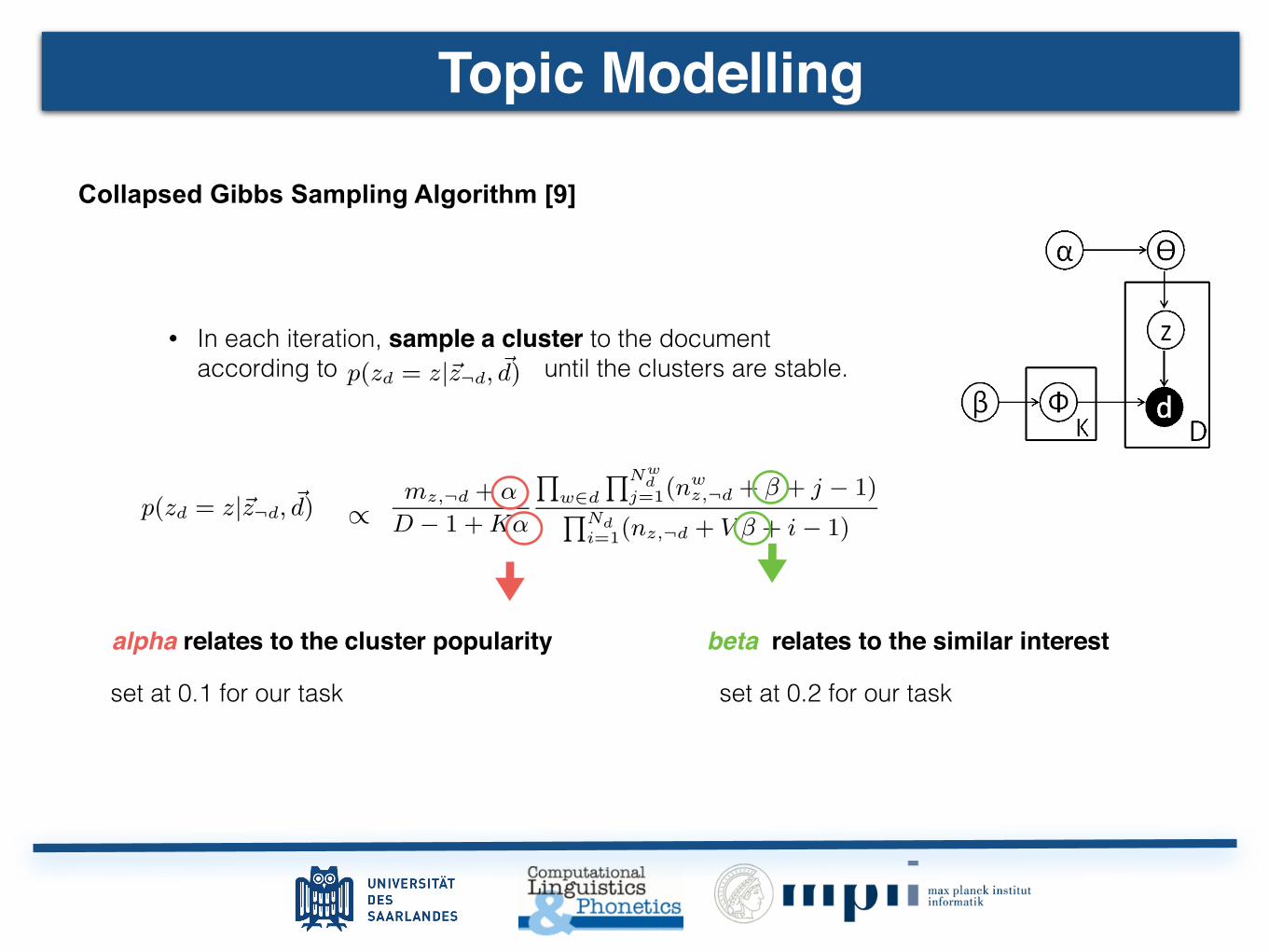
Topic Modeling
Collapsed Gibbs Sampling Algorithm [9]
Figure 1: Graphical model of DMM.
V number of words in the vocabularyD number of documents in the corpusL average length of documentsd documents in the corpusz cluster labels of each documentI number of iterationsmz number of documents in cluster z
nz number of words in cluster z
nwz number of occurrences of word w in cluster z
Nd number of words in document d
Nwd number of occurrences of word w in document d
Table 1: Notations
probability over all mixture components:
p(d) =K!
k=1
p(d|z = k)p(z = k) (1)
Here, K is the number of mixture components (clusters).Now, the problem becomes how to define p(d|z = k) andp(z = k). DMM makes the Naive Bayes assumption: thatthe words in a document are generated independently whenthe document’s cluster label k is known, and the probabilityof a word is independent of its position within the document.Then the probability of document d generated by cluster kcan be derived as follows:
p(d|z = k) ="
w∈d
p(w|z = k) (2)
Nigam et al. [20] assumes that each mixture component(cluster) is a multinomial distribution over words, such thatp(w|z = k) = p(w|z = k,Φ) = φk,w, where w = 1, ..., Vand
#w φk,w = 1. They assume a Dirichlet distribution as
the prior for each mixture component (cluster), such that
p(Φ|β) = Dir(φk|β). They also assume that the weight ofeach mixture component (cluster) is sampled from a multi-nomial distribution, such that p(z = k) = p(z = k|Θ) = θk,where k = 1, ..., K and
#k θk = 1. In addition, they assume
a Dirichlet prior for this multinomial distribution, such thatp(Θ|α) = Dir(θ|α).
The graphical model of DMM is shown in Figure 1. Inour short text clustering problem, we need to estimate themixture component (cluster) z for each document d. Wewill introduce our GSDMM algorithm with the help of theMovie Group Process (MGP) in the next section.
2.3 Gibbs Sampling for DMMIn this section, we introduce the collapsed Gibbs Sampling
algorithm for the Dirichlet Multinomial Mixture model (ab-br. to GSDMM), which is equivalent to the Movie GroupProcess (MGP) introduced in Section 2.1.
The detail of our GSDMM algorithm is shown in Algo-rithm 1, and the meaning of its variables is shown in Table1. In the initialization step, we randomly assign the docu-
ments to K clusters, and record the following information:z (cluster labels of each document), mz (number of docu-ments in cluster z), nz (number of words in cluster z), andnwz (number of occurrences of word w in cluster z). Then
we traverse the documents for I iterations. (In Section 4.4,we found that GSDMM can achieve good and stable perfor-mance when I equals five.) In each iteration, we re-assigna cluster for each document d in turn according to the con-ditional distribution: p(zd = z|z¬d, d), where ¬d means thecluster label of document d is removed from z. Each timewe re-assign a cluster z to document d, the correspondinginformation in z, mz, nz, and nw
z are updated accordingly.Finally, only a part of the initial K clusters will remain non-empty, in other words, GSDMM can cluster the documentsinto several groups. Through experimental study in Section4.5, we found that the number of non-empty clusters foundby GSDMM can be near the true number of groups as longas K is larger than the true number. GSDMM is also a softclustering model like Gaussian Mixture Model (GMM) [5],since we can get the probability of each document belongingto each cluster from p(zd = z|z¬d, d).
Algorithm 1: GSDMM
Data: Documents in the input, d.Result: Cluster labels of each document, z.begin
initialize mz, nz, and nwz as zero for each cluster z
for each document d ∈ [1, D] dosample a cluster for d:zd ← z ∼Multinomial(1/K)mz ← mz + 1 and nz ← nz +Nd
for each word w ∈ d donwz ← nw
z +Nwd
for i ∈ [1, I ] dofor each document d ∈ [1, D] do
record the current cluster of d: z = zdmz ← mz − 1 and nz ← nz −Nd
for each word w ∈ d donwz ← nw
z −Nwd
sample a cluster for d:zd ← z ∼ p(zd = z|z¬d, d) (Equation 4)mz ← mz + 1 and nz ← nz +Nd
for each word w ∈ d donwz ← nw
z +Nwd
We can derive p(zd = z|z¬d, d) from the Dirichlet Multi-nomial Mixture (DMM) model, and find that it conformsto the two rules of MGP introduced in Section 2.1. Wejust introduce the results directly here, and will explain thederivation details in the next section.
If we assume each word can at most appear once in eachdocument (In the movie group example, the assumption isthat a movie can at most appear once in each student’slist). We can derive a quite elegant form of the conditionaldistribution as follows:
p(zd = z|z¬d, d) ∝
mz,¬d + αD − 1 +Kα
$w∈d(n
wz,¬d + β)
$Ndi=1(nz,¬d + V β + i− 1)
(3)
235
• In each iteration, sample a cluster to the document according to until the clusters are stable.
where Nd is the number of words in document d. In shorttext setting, Nd is often less than 100.
The first part of Equation 3 relates to Rule 1 of MG-P (Choose a table with more students). Here mz,¬d is thenumber of students (documents) in table z without consider-ing student d, and D is the total number of students. Whentable z has more students, the first part tends to be larger,and a student will tend to choose a table with more students.As a result, the first part of Equation 3 tends to result inlarge completeness, because it leads large tables (clusters)to be larger and students in the same ground true group aremore likely to be in the same table (cluster). The secondpart of Equation 3 relates to Rule 2 of MGP (Choose a ta-ble whose students share similar interests with him). Herenwz,¬d and nz,¬d are the number of occurrences of movie w
in table z and the total number of movies in table z with-out considering student d, respectively. When table z hasmore students sharing similar interests with student d (i.e.,watched more movies of the same), movies of student d willappear more often in table z (with larger nw
z,¬d), and theprobability of student d choosing table z will be larger. Asa result, the second part of Equation 3 tends to result inlarge homogeneity, because it can leads the students in thesame table to be more similar (more likely to be in the sameground true group).
If we allow a word to appear multi-times in a document(A movie can appear multi-times in a student’s list). Wecan derive the conditional probability as follows:
p(zd = z|z¬d, d) ∝
mz,¬d + αD − 1 +Kα
!w∈d
!Nwd
j=1(nwz,¬d + β + j − 1)
!Ndi=1(nz,¬d + V β + i− 1)
(4)
where Nwd is the number of occurrences of word w in doc-
ument d. We should note that the two parts of Equation 4have similar relationship with MGP like that of Equation 3,and the complexity of Equation 4 is the same as Equation 3.The only difference between them is the numerator of theirsecond part. We will try to derive Equation 3 and Equation4 from the Dirichlet Multinomial Mixture (DMM) model inthe next section.
2.4 Derivation of GSDMMIn this section, we try to formally derive the conditional
distribution p(zd = z|z¬d, d) used in our GSDMM algorithmas follows.
p(zd = z|z¬d, d) =p(d, z|α, β)
p(d, z¬d|α, β)∝
p(d, z|α, β)
p(d¬d, z¬d|α, β)(5)
where ¬d means document d is excluded from z and d. Nowwe need to derive the full distribution p(d, z|α, β). From the
graphical model of DMM in Figure 1, we can see p(d, z|α, β) =
p(d|z, β)p(z|α). Then we need to derive p(d|z, β) and p(z|α).Let us first investigate how to obtain p(z|α). We can see
that p(z|α) can be obtained by integrating with respect toΘ as p(z|α) =
"p(z|Θ)p(Θ|α)dΘ. As mentioned in Sec-
tion 2.2, p(Θ|α) is a Dirichlet distribution and p(z|Θ) isa multinomial distribution. With similar techniques of [9],
we can get p(z|α) = ∆(m+α)∆(α) , where m = {mk}
Kk=1, and
mk is the number of documents (students) in the kth clus-ter (table). Here we adopt the ∆ function in [9], and we
have ∆(α) =!K
k=1Γ(α)
Γ("
Kk=1
α)and ∆(m + α) =
!Kk=1
Γ(mk+α)
Γ("
Kk=1
(mk+α))=
!Kk=1
Γ(mk+α)Γ(D+Kα) , where D is the number of documents in the
dataset, D =#K
k=1 mk.
Similarly, p(d|z, β) can be obtained by integrating with re-
spect to Φ as p(d|z, β) ="p(d|z,Φ)p(Φ|β)dΦ =
!Kk=1
∆(nk+β)
∆(β),
where nk = {nwk }
Vw=1, and nw
k is the number of occurrences
of word w in the kth cluster (table). Similarly, ∆(β) =!V
w=1Γ(β)
Γ("
Vw=1
β)and∆(nk+β) =
!Vw=1
Γ(nwk +β)
Γ("
Vw=1
(nwk+β))
=!V
w=1Γ(nw
k +β)Γ(nk+V β) ,
where nk is number of words (movies) in document (table)k, that is, nk =
#Vw=1 n
wk .
Now the joint distribution becomes:
p(d, z|α, β) =∆(m+ α)
∆(α)
K$
k=1
∆(nk + β)
∆(β)
Then the conditional distribution in Equation 5 can be de-rived as follows:
p(zd = z|z¬d, d) ∝p(d, z|α, β)
p(d¬d, z¬d|α, β)
∝∆(m+ α)
∆(m¬d + α)∆(nz + β)
∆(nz,¬d + β)
∝Γ(mz + α)
Γ(mz,¬d + α)Γ(D − 1 +Kα)Γ(D +Kα)!
w∈d Γ(nwz + β)!
w∈d Γ(nwz,¬d + β)
Γ(nz,¬d + V β)Γ(nz + V β)
(6)
where mz = mz,¬d + 1 and nz = nz,¬d + Nd. Because Γ
function has the following property: Γ(x+m)Γ(x) =
!mi=1(x+ i−
1). We can rewrite Equation 6 into the following form:
p(zd = z|z¬d, d)
∝mz,¬d + αD − 1 +Kα
!w∈d Γ(nw
z +β)!
w∈d Γ(nwz,¬d
+β)!Nd
i=1(nz,¬d + V β + i− 1)(7)
When we assume each word can at most appear once ineach document (In the movie group example, the assumptionis a movie can at most appear once in each student’s list).
We can get!
w∈d Γ(nwz +β)
!w∈d Γ(nw
z,¬d+β) =
!w∈d(n
wz,¬d + β) since nw
z =
nwz,¬d +1 holds, and Equation 7 turns out to be Equation 3.When we allow a word to appear multi-times in each doc-
ument (A movie can appear multi-times in each student’s
list).We can get!
w∈d Γ(nwz +β)
!w∈d Γ(nw
z,¬d+β) =
!w∈d
!Nwd
j=1(nwz,¬d + β +
j − 1) since nwz = nw
z,¬d +Nwd holds, and Equation 7 turns
out to be Equation 4.
3. DISCUSSION
3.1 Meaning of Alpha and BetaIn this part, we try to explore the meaning of α and β with
the help of the Movie Group Process (MGP) as introducedin Section 2.1. From Equation 4, we can see that α relatesto the prior probability of a student (document) choosing atable (cluster). If we set α = 0, a table will never be chosenby the students once it gets empty, because the first part ofEquation 4 is now zero. When α gets larger, the probabilityof a student choosing an empty table will also gets larger.
236
alpha relates to the cluster popularity beta relates to the similar interest
Topic Modelling
where Nd is the number of words in document d. In shorttext setting, Nd is often less than 100.
The first part of Equation 3 relates to Rule 1 of MG-P (Choose a table with more students). Here mz,¬d is thenumber of students (documents) in table z without consider-ing student d, and D is the total number of students. Whentable z has more students, the first part tends to be larger,and a student will tend to choose a table with more students.As a result, the first part of Equation 3 tends to result inlarge completeness, because it leads large tables (clusters)to be larger and students in the same ground true group aremore likely to be in the same table (cluster). The secondpart of Equation 3 relates to Rule 2 of MGP (Choose a ta-ble whose students share similar interests with him). Herenwz,¬d and nz,¬d are the number of occurrences of movie w
in table z and the total number of movies in table z with-out considering student d, respectively. When table z hasmore students sharing similar interests with student d (i.e.,watched more movies of the same), movies of student d willappear more often in table z (with larger nw
z,¬d), and theprobability of student d choosing table z will be larger. Asa result, the second part of Equation 3 tends to result inlarge homogeneity, because it can leads the students in thesame table to be more similar (more likely to be in the sameground true group).
If we allow a word to appear multi-times in a document(A movie can appear multi-times in a student’s list). Wecan derive the conditional probability as follows:
p(zd = z|z¬d, d) ∝
mz,¬d + αD − 1 +Kα
!w∈d
!Nwd
j=1(nwz,¬d + β + j − 1)
!Ndi=1(nz,¬d + V β + i− 1)
(4)
where Nwd is the number of occurrences of word w in doc-
ument d. We should note that the two parts of Equation 4have similar relationship with MGP like that of Equation 3,and the complexity of Equation 4 is the same as Equation 3.The only difference between them is the numerator of theirsecond part. We will try to derive Equation 3 and Equation4 from the Dirichlet Multinomial Mixture (DMM) model inthe next section.
2.4 Derivation of GSDMMIn this section, we try to formally derive the conditional
distribution p(zd = z|z¬d, d) used in our GSDMM algorithmas follows.
p(zd = z|z¬d, d) =p(d, z|α, β)
p(d, z¬d|α, β)∝
p(d, z|α, β)
p(d¬d, z¬d|α, β)(5)
where ¬d means document d is excluded from z and d. Nowwe need to derive the full distribution p(d, z|α, β). From the
graphical model of DMM in Figure 1, we can see p(d, z|α, β) =
p(d|z, β)p(z|α). Then we need to derive p(d|z, β) and p(z|α).Let us first investigate how to obtain p(z|α). We can see
that p(z|α) can be obtained by integrating with respect toΘ as p(z|α) =
"p(z|Θ)p(Θ|α)dΘ. As mentioned in Sec-
tion 2.2, p(Θ|α) is a Dirichlet distribution and p(z|Θ) isa multinomial distribution. With similar techniques of [9],
we can get p(z|α) = ∆(m+α)∆(α) , where m = {mk}
Kk=1, and
mk is the number of documents (students) in the kth clus-ter (table). Here we adopt the ∆ function in [9], and we
have ∆(α) =!K
k=1Γ(α)
Γ("
Kk=1
α)and ∆(m + α) =
!Kk=1
Γ(mk+α)
Γ("
Kk=1
(mk+α))=
!Kk=1
Γ(mk+α)Γ(D+Kα) , where D is the number of documents in the
dataset, D =#K
k=1 mk.
Similarly, p(d|z, β) can be obtained by integrating with re-
spect to Φ as p(d|z, β) ="p(d|z,Φ)p(Φ|β)dΦ =
!Kk=1
∆(nk+β)
∆(β),
where nk = {nwk }
Vw=1, and nw
k is the number of occurrences
of word w in the kth cluster (table). Similarly, ∆(β) =!V
w=1Γ(β)
Γ("
Vw=1
β)and∆(nk+β) =
!Vw=1
Γ(nwk +β)
Γ("
Vw=1
(nwk+β))
=!V
w=1Γ(nw
k +β)Γ(nk+V β) ,
where nk is number of words (movies) in document (table)k, that is, nk =
#Vw=1 n
wk .
Now the joint distribution becomes:
p(d, z|α, β) =∆(m+ α)
∆(α)
K$
k=1
∆(nk + β)
∆(β)
Then the conditional distribution in Equation 5 can be de-rived as follows:
p(zd = z|z¬d, d) ∝p(d, z|α, β)
p(d¬d, z¬d|α, β)
∝∆(m+ α)
∆(m¬d + α)∆(nz + β)
∆(nz,¬d + β)
∝Γ(mz + α)
Γ(mz,¬d + α)Γ(D − 1 +Kα)Γ(D +Kα)!
w∈d Γ(nwz + β)!
w∈d Γ(nwz,¬d + β)
Γ(nz,¬d + V β)Γ(nz + V β)
(6)
where mz = mz,¬d + 1 and nz = nz,¬d + Nd. Because Γ
function has the following property: Γ(x+m)Γ(x) =
!mi=1(x+ i−
1). We can rewrite Equation 6 into the following form:
p(zd = z|z¬d, d)
∝mz,¬d + αD − 1 +Kα
!w∈d Γ(nw
z +β)!
w∈d Γ(nwz,¬d
+β)!Nd
i=1(nz,¬d + V β + i− 1)(7)
When we assume each word can at most appear once ineach document (In the movie group example, the assumptionis a movie can at most appear once in each student’s list).
We can get!
w∈d Γ(nwz +β)
!w∈d Γ(nw
z,¬d+β) =
!w∈d(n
wz,¬d + β) since nw
z =
nwz,¬d +1 holds, and Equation 7 turns out to be Equation 3.When we allow a word to appear multi-times in each doc-
ument (A movie can appear multi-times in each student’s
list).We can get!
w∈d Γ(nwz +β)
!w∈d Γ(nw
z,¬d+β) =
!w∈d
!Nwd
j=1(nwz,¬d + β +
j − 1) since nwz = nw
z,¬d +Nwd holds, and Equation 7 turns
out to be Equation 4.
3. DISCUSSION
3.1 Meaning of Alpha and BetaIn this part, we try to explore the meaning of α and β with
the help of the Movie Group Process (MGP) as introducedin Section 2.1. From Equation 4, we can see that α relatesto the prior probability of a student (document) choosing atable (cluster). If we set α = 0, a table will never be chosenby the students once it gets empty, because the first part ofEquation 4 is now zero. When α gets larger, the probabilityof a student choosing an empty table will also gets larger.
236
set at 0.1 for our task set at 0.2 for our task

Topic Modeling Dirichlet Multinomial Mixture Model (DMM) and collapsed Gibbs Sampling algorithm
• The number of clusters is inferred automatically • Balance the completeness and homogeneity of the clusters • Converge fast • Cope with the sparse and high- dimensional problem of short texts • Representative words of each cluster (similar to PLSA and LDA ) are the most frequent words in each cluster.
We get excellent results, majority of the topic clusters can be easily interpreted using the representative words.
For the thread Germany won the world cup in Brazil, some comments are in Portuguese and German. Our topic modelling approach can cluster the comments according to the language, so we get a cluster of comments in German and a cluster in Portuguese.
Topic Modelling

Topic Modeling
Rank:
Rank:
Rank: K
Thread
Thread
ThreadRank:
Thread Extract 27 topical Clusters
Topic 1
Topic 2
Topic 3
Topic k
Query: December 17 2014 – U.S. President Barack Obama announces the resumption of normal relations between the U.S. and Cuba.
2691 comments from the top 10 threads
Topic Modelling Example:

Topic Modeling
• Obama announces historic overhaul of relations; Cuba releases American• Cuba Wants Off U.S. Terrorism List Before Restoring Normal Ties• Most Americans Support Renewed U.S.-Cuba Relations• Raul Castro: US Must Return Guantanamo for Normal Relations• Russian foreign minister praises new U.S.-Cuba relations• U.S. Approves Ferry Service Between Florida and Cuba• US, Cuba restore full diplomatic relations after 54 years• President Barack Obama announced Wednesday that the U.S. and Cuba
will reopen their embassies in Havana and Washington, heralding a "new chapter" in relations after a half-century of hostility.
• Raul Castro: U.S. must return Guantanamo for normal relations• U.S. Takes Cuba off Terror List, Paving the Way for Normal Ties
Although the Top 10 threads are all about Cuba and the US
Topic Modelling

Clustering 27 topical clusters extracted from 2691 comments for the query:
Number of Comments Topic Words ( Top 10 most frequent words)
8 18 war libya utf partagas haiti 69i god somalia isil pakistan12 7 cuban statistic government cuba un mean have independent number ha11 21 mexico cuba gulf gitmo america gtmo navy panamacanal small control10 22 ftfy nixon cheney nato un germany lincoln still facebook republican13 57 tropico isi terrorist just know order have people cia drone38 218 cuba america cia germany turkey have soviet japan castro war15 101 russia ukraine america cuba russian crimea have american eu state14 240 cuban cigar cuba have tobacco people nicaragua so just dominican17 10 southafrica angola cuba south africa mozambique death get un leonardcohen18 155 cuba america canada country american mexico list china ha saudi30 6 nonmobile pollo jadehelm15 feedback mobile please counter bot non link37 530 have just re people think american thing up that so32 416 cuba cuban guantanamo american government have us castro lease country
Topic Index
More relevant topics in their linked comments are discovered.
Topic Modelling
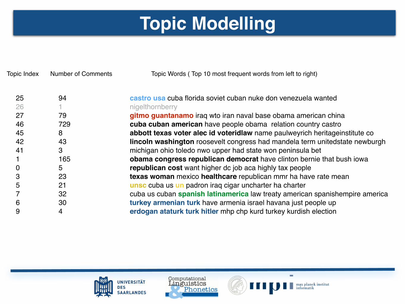
Clustering
Number of Comments Topic Words ( Top 10 most frequent words from left to right)
25 94 castro usa cuba florida soviet cuban nuke don venezuela wanted26 1 nigelthornberry 27 79 gitmo guantanamo iraq wto iran naval base obama american china46 729 cuba cuban american have people obama relation country castro45 8 abbott texas voter alec id voteridlaw name paulweyrich heritageinstitute co42 43 lincoln washington roosevelt congress had mandela term unitedstate newburgh41 3 michigan ohio toledo nwo upper had state won peninsula bet1 165 obama congress republican democrat have clinton bernie that bush iowa0 5 republican cost want higher dc job aca highly tax people3 23 texas woman mexico healthcare republican mmr ha have rate mean5 21 unsc cuba us un padron iraq cigar uncharter ha charter7 32 cuba us cuban spanish latinamerica law treaty american spanishempire america6 30 turkey armenian turk have armenia israel havana just people up9 4 erdogan ataturk turk hitler mhp chp kurd turkey kurdish election
Topic Index
Topic Modelling

Solution Overview
elastic search system
text processing topic modelling diversification
• Top k threads • Topic Tagging
• Topic Extraction
• Text Normalisation
• Named Entity Tagging
• Text Representation
• Sentiment Tagging
• Sainte Laguë Method
• Comments Tree
Decomposition

ThreadRank ThreadRank
label the comments from each thread then each thread has n topic clusters of comments Diversification -Sainte Laguë Method
topic 1
topic 2
topic 3
po

ThreadRank ThreadRank
label every comment a sentiment label or an emotional label (if emotion modelling works)
Positive
Neutral
Negative
Diversification -Sainte Laguë Method

Diversification -Sainte Laguë MethodThreadRank
po
ThreadRank
topic 1
topic 2
topic 3

po
Thread
Diversification -Sainte Laguë Method

Diversification -Sainte Laguë MethodSainte Laguë Method
7 Diversification Methods
7.0.1 Sainte-Lague Method
In situations where the comments do not follow conversational style, they can be treated
as independent entities. Zhao’s study [69] shows that one characteristic of social media
content compared with traditional news media is the amount and coverage of user opinions
expressed. Therefore, in addition to the topic aspect of the comment, we also create a sen-
timent dimension for each comment. That way, a comment ci,j
(ci,j
2 C
i
) is labeled with a
topic tag topic
ci,j and a sentiment tag senti
ci,j . The reason why we add the sentiment di-
mension when comments are treated as independent entities is that a single comment has
only one sentiment; However, when the conversation style is considered, the discussions of
tree-structured comments are treated as entities so that generally discussions present all
the three sentiments namely positive, negative and neutral. We choose VADER [32] for
the sentiment analysis task. VADER uses a combination of qualitative and quantitative
methods to produce empirically validate, valence-based, gold-standard sentiment lexicon
which is especially attuned to social media texts. Each comment ci,j
has a score sci,j given
by users and a pseudo relevance score spr,i
that Ci
inherits from t
i
. For each of the threads
t
i
(ti
2 T, |T | = m), we cluster the linked comments Ci
(Ci
2 C) according to both of the
tags (topicci,j , sentici,j); Then we first rank the all the topic-sentiment clusters according
to the pseudo relevance score s
pr,i
so for each rank r
j
(rj
2 R, |R| = |T | = m), there are
a number of Ncl,rj topic-sentiment clusters cl
i,rj (cli,rj 2 Lr
j
, |Lrj
| = N
cl,rj); Second we
rank the comments in each of the topic-sentiment clusters cli,rj according to the score s
ci,j
given by users.
Here we propose the Sainte-Lague (SL) method to diversify the search result by re-
trieving the representative comments proportionally from Lr
j
. SL method [38] is a high-
est quotient method for allocating seats in party-list proportional representation used in
many voting systems. After all the comments have been tallied, successive quotients are
computed using equation 11 for each cluster. where, V is the total number of comments
in each cluster; S is the number of ’seats’ that cluster has been allocated so far, initially
0 for all clusters.
quotient =V
2S + 1(11)
Whichever cluster has the highest quotient gets the next ’seat’ allocated, and their quo-
tient is recalculated given their new ’seat’ total. The process is repeated until all ’seats’
have been allocated. The number of the ’seats’ is a hyper-parameter, it can be set accord-
ing to users’ interests. We use table 2 as an example illustrates how the process works:
There are three clusters. five comments are expected to be retrieved (number of ’seats’
is five). The denominators in the first row are calculated as 2S + 1 where S = 0, 1, 2...
respectively and the quotients in the column 2 to column 4 are the quotients calculated
32
The Sainte Laguë Method is a highest quotient method for allocating seats in party-list proportional representation used in many voting systems.
After all the comments have been tallied, successive quotients are computed for each cluster. where, • V is the total number of comments in each cluster; • S is the number of ’seats’ that cluster has been allocated so far, initially 0
for all clusters

poThread
Diversification -Sainte Laguë Method
Denominator /1 /3 /5 Seats(*)
topic A positive 50* 16.67* 10 2
topic A neutral 40* 13.33* 8 2
topic A negative 30* 10 6 1
Table 2. Sainte-Lague method example
• Lastly we retrieve n comments proportionally from the diverse clusters to form the
final result which is concise and diverse as Figure 10.
Figure 10. Final Retrieval Result
We apply SL method to clusters Lrj of all ranks. Comments c
g
with higher user score
s
ci,j are selected first. Nrj is the number of retrieved comments (’seats’) at rank r
j
(rj
2 R)
and
N
rj = min(� ·Ncl,rj , |C
i,rj |)
where, � is a positive constant controlling the retrieval scale. |Ci,rj | is number of comments
C
i
at rank j. Then the representative comments are retrieved from each topic-sentiment
cluster of all ranks proportionally.
36
Example:
5 comments are expected to be retrieved (number of ‘seats’ is 5). The denominators in the first row are calculated as 2S + 1 where S = 0, 1, 2... respectively and the quotients in the column 2 to column 4 are the quotients calculated. The quotients marked with “*” represent the allocated ‘seats’.
So for this example,
2 comments are from cluster topic A positive
2 comments from cluster topic A neutral 1 comment from cluster topic A negative
are retrieved
7 Diversification Methods
7.0.1 Sainte-Lague Method
In situations where the comments do not follow conversational style, they can be treated
as independent entities. Zhao’s study [69] shows that one characteristic of social media
content compared with traditional news media is the amount and coverage of user opinions
expressed. Therefore, in addition to the topic aspect of the comment, we also create a sen-
timent dimension for each comment. That way, a comment ci,j
(ci,j
2 C
i
) is labeled with a
topic tag topic
ci,j and a sentiment tag senti
ci,j . The reason why we add the sentiment di-
mension when comments are treated as independent entities is that a single comment has
only one sentiment; However, when the conversation style is considered, the discussions of
tree-structured comments are treated as entities so that generally discussions present all
the three sentiments namely positive, negative and neutral. We choose VADER [32] for
the sentiment analysis task. VADER uses a combination of qualitative and quantitative
methods to produce empirically validate, valence-based, gold-standard sentiment lexicon
which is especially attuned to social media texts. Each comment ci,j
has a score sci,j given
by users and a pseudo relevance score spr,i
that Ci
inherits from t
i
. For each of the threads
t
i
(ti
2 T, |T | = m), we cluster the linked comments Ci
(Ci
2 C) according to both of the
tags (topicci,j , sentici,j); Then we first rank the all the topic-sentiment clusters according
to the pseudo relevance score s
pr,i
so for each rank r
j
(rj
2 R, |R| = |T | = m), there are
a number of Ncl,rj topic-sentiment clusters cl
i,rj (cli,rj 2 Lr
j
, |Lrj
| = N
cl,rj); Second we
rank the comments in each of the topic-sentiment clusters cli,rj according to the score s
ci,j
given by users.
Here we propose the Sainte-Lague (SL) method to diversify the search result by re-
trieving the representative comments proportionally from Lr
j
. SL method [38] is a high-
est quotient method for allocating seats in party-list proportional representation used in
many voting systems. After all the comments have been tallied, successive quotients are
computed using equation 11 for each cluster. where, V is the total number of comments
in each cluster; S is the number of ’seats’ that cluster has been allocated so far, initially
0 for all clusters.
quotient =V
2S + 1(11)
Whichever cluster has the highest quotient gets the next ’seat’ allocated, and their quo-
tient is recalculated given their new ’seat’ total. The process is repeated until all ’seats’
have been allocated. The number of the ’seats’ is a hyper-parameter, it can be set accord-
ing to users’ interests. We use table 2 as an example illustrates how the process works:
There are three clusters. five comments are expected to be retrieved (number of ’seats’
is five). The denominators in the first row are calculated as 2S + 1 where S = 0, 1, 2...
respectively and the quotients in the column 2 to column 4 are the quotients calculated
32

Diversification -Sainte Laguë Method
We apply SL method to clusters of all ranks. Comments with higher user score are selected first.
retrieval number = min ( γ · Ncl,rj , |Ci,rj | )
• Nrj is the number of retrieved comments at rank rj (rj ∈ R)
• γ is a positive constant controlling the retrieval scale.
• |Ci,rj | is number of comments Ci at rank j.
• Then the representative comments are retrieved from each topic-sentiment cluster of all ranks proportionally.
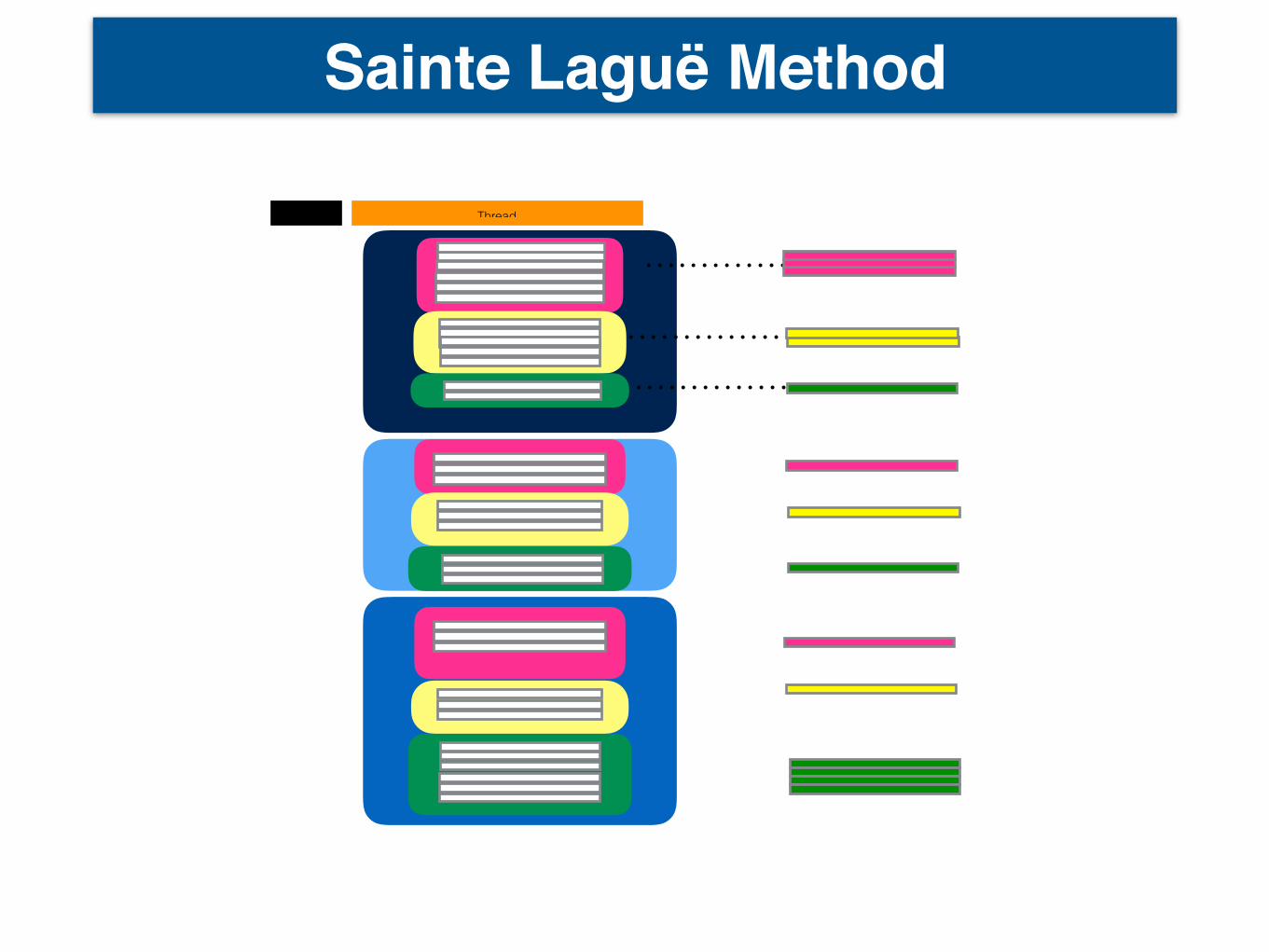
Sainte Laguë Method
po
Thread

po
po
po
rank 1
rank 2
rank 3
Diversified Search Result
Pseudo Search Result

Comments Tree Decomposition
THREADRank
Comments Tree
• Levels (with different colors) represents the coherence: • comment at lower level is the reply to the one at higher level • comments at the same level are independent.

Comments Tree Decomposition
THREADRank
Comments Tree
Set the Decomposition level at 1,

Comments Tree Decomposition
comment level 0
comment level 1 comment level 1
comment level 2comment level 2 comment level 2
comment level 3
comment level 4 comment level 4
comment level 3
enumerate the path from level 0 to level m

Comments Tree Decomposition
comment level 0
comment level 1 comment level 1
comment level 2comment level 2 comment level 2
comment level 3
comment level 4 comment level 4
comment level 3sub-tree 1

Comments Tree Decomposition
comment level 0
comment level 1 comment level 1
comment level 2comment level 2 comment level 2
comment level 3
comment level 4 comment level 4
comment level 3
sub-tree 2
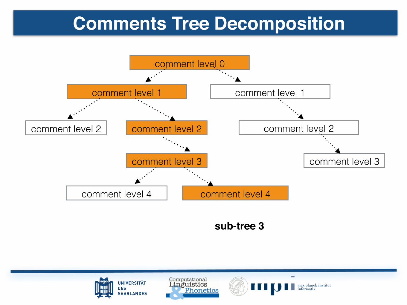
Comments Tree Decomposition
comment level 0
comment level 1 comment level 1
comment level 2comment level 2 comment level 2
comment level 3
comment level 4 comment level 4
comment level 3
sub-tree 3

Comments Tree Decomposition
comment level 0
comment level 1 comment level 1
comment level 2comment level 2 comment level 2
comment level 3
comment level 4 comment level 4
comment level 3
sub-tree 4

Example : Query: December 17 2014 – U.S. President Barack Obama announces the resumption of normal relations between the U.S. and Cuba.
• When decomposition level is set at 5, the number of the sub-trees for each retrieved thread is as follows:
thread1 thread2 thread3 thread4 thread5 thread6 thread7 thread8 thread9 thread10
number of trees (per thread) 1 8 8 3 15 49 90 2 127 11
number of decomposed sub-trees trees (per thread) 1 19 17 3 35 165 342 2 625 11
Comments Tree Decomposition

Sub-Tree 1
Sub-Tree 2
Select one sub-tree according to the sub-tree score
Comments Tree Decomposition

Comments Tree Decomposition
• Comment Score: each comment has a score given by users. Sub-tree score is the sum of the user score of the comments in the subtree.
• Linguistic Features: score the subtree using the diversity of the linguistic feature of each comment in the subtree. The different linguistic features we propose are NP words (words that can potentially form noun phrases), named entities and bigrams.
• Number of Topics: diversity of the topic tag of comment in the sub-tree.

Experiment Setup
Data: 26,669,242 Reddit comments 845,004 threads from year 2008-2015
Sub-reddit: worldnews / politics
Queries: 50 news summaries from Wikinews 2011-2014
Ranking: Elasticsearch and Okapi BM-25 score ranking and choose the top 10 threads and their linked comments; on average there are 4330.7 comments retrieved for each query.

Experiment Evaluation
• We use Cumulative Gain (CG) to measure the diversity, CG can also penalise redundancy.
• Charles L.A claims [7] that CG at rank k can be used directly as diversity evaluation measure.
• Al-maskari [8] provides evidence that CG correlates better with user satisfaction than Normalised Discounted Cumulative Gain (nDCG).

Experiment Evaluation
8 Experimental Evaluation
We conducted our experiment using the Reddit data from year 2008 to 2015 which consists
of 845, 004 threads and their 26, 669, 242 linked comments; 50 queries are news summaries
from Wikinews from year 2011 to 2014.
We use elastic search [26] with Okapi BM 25 [39] retrieve and rank the threads and
choose the top 10 threads as well as their linked comments as pseudo search result (R)
for each query. There are 4436.43 comments on average for each query. Then we carried
out the following tasks for the pseudo search result (R) of each query:
• text pre-processing: normalize the comments for each query following the steps
in section 4.1.
• topic modeling : extract the topics from each pseudo returned result R using
the technique as described in section 4.2. We set ↵ = 0.1 and � = 0.2 in order to
extract more interpretable topics after examining manually the all topic words; We
also notice comments of di↵erent languages are clustered according to the language,
which shows the robustness of our topic modeling technique. Then each comment
is labeled with a topic tag.
• sentiment analysis use VADER as discussed in section 4.4 to give a score for each
comment for the Sainte-Lague method. We label the comment using compound
score and label a positive tag when the score is between 1 and 0.1, a negative tag
when it is between �0.1 and �1 or a neutral tag when it falls in between 0.2 and
�0.2.
We use Cumulative Gain (CG) to measure the diversity and CG also penalizes redun-
dancy:
CG[k] =kX
j=1
G[j] (12)
G[k] =mX
i=1
J(dk
, i)(1� ↵)ri,k�1 (13)
where, ri,k�1 is the number of comments (d
j
) ranked up to position k � 1 that contain
nugget ni
and
r
i,k�1 =k�1X
j=1
J(dj
, i)
39
where,
Document Title 85.1 85.2 85.3 85.4 85.5 85.6 Totala. Carnival Re-Enters Norway Bidding X X 2b. NORWEGIAN CRUISE LINE SAYS OUTLOOK IS GOOD X 1c. Carnival, Star Increase NCL Stake X 1d. Carnival, Star Solidify Control 0e. HOUSTON CRUISE INDUSTRY GETS BOOST WITH... X X 2f. TRAVELERS WIN IN CRUISE TUG-OF-WAR X 1g. ARMCHAIR QUARTERBACKS NEED... THIS CRUISE X 1h. EUROPE, CHRISTMAS ON SALE X 1i. TRAVEL DEALS AND DISCOUNTS 0j. HAVE IT YOUR WAY ON THIS SHIP 0
Table 2: Top ten documents returned for the query“Norwegian Cruise Lines (NCL)”. The questions answeredby each document are indicated.
also of ni ∈ d and nj =i ∈ d. Under this assumption, Equa-tion 1 may be rewritten
P (R = 1|u, d) = 1 −m
Y
i=1
(1 − P (ni ∈ u) · P (ni ∈ d)). (2)
Next, we turn our attention to the problem of estimat-ing P (ni ∈ u) and P (ni ∈ d). With respect to the user,we are making the strong assumption that a user’s interestin one nugget is independent of other nuggets. We discussthe ramifications of this assumption further in Section 4.2.We then consider ranked lists, where the relevance of eachsubsequent element is conditioned on the preceding ones.
4.1 Relevance JudgmentsTo estimate P (ni ∈ d) we adopt a simple model inspired
by the manual judgments typical of TREC tasks. We as-sume that a human assessor reads d and reaches a binarydecision regarding each nugget: Is the nugget contained inthe document or not?
Let J(d, i) = 1 if the assessor has judged that d containsnugget ni, and J(d, i) = 0 if not. A possible estimate forP (ni ∈ d) is then:
P (ni ∈ d) =
ȷ
α if J(d, i) = 1,0 otherwise.
(3)
The value α is a constant with 0 < α ≤ 1, which reflectsthe possibility of assessor error. This definition assumesthat positive judgments may be erroneous, but that nega-tive judgments are always correct. This definition is a crudeapproximation of reality, but is still a step beyond the tra-ditional assumption of perfect accuracy. More sophisticatedestimates are possible, but are left for future work. If weassume Equation 3, then Equation 2 becomes:
P (R = 1|u, d) = 1 −m
Y
i=1
(1 − P (ni ∈ u)αJ(d, i)) . (4)
4.2 Ambiguity and DiversityIn arguing for evaluation methodologies that address query
ambiguity, Sparck Jones et al. [25] emphasize that queries“are linguistically ambiguous, not just in the classic sense ofwords with multiple senses present in a dictionary, but alsoambiguous across place names, person names, acronyms,etc.” A number of researchers have investigated the rela-tionship between query ambiguity and query difficulty [4,14, 19]. Cronen-Townsend et al. [14] view ambiguity as a
property that is inherent to a query “with respect to the col-lection being searched”. They develop and validate a clarityscore, based on the K-L divergence between a query languagemodel and the collection language model. Their query lan-guage model is constructed from the top-ranked documentsreturned by the query. The clarity score is intended to re-flect the coherence of these documents: Are they about asingle topic or a mixture of topics?
In part, ambiguity may be associated with dependenciesbetween the nuggets, which are ignored by Equation 2. Whilea user interested in the Norwegian Cruise Lines may find anyfact regarding the company useful, the same cannot be saidfor our Web search example. A user interested in the parcelservice will be less interested in nuggets related to powersupplies.
An evaluation measure intending to reward diversity musttake these dependencies into account when estimating P (ni ∈u). In the case of our Web search example, we identifiedthree possible interpretations of the query. Assuming ourintuition regarding the user population is correct, nuggetsrelated to the parcel service must be assigned substantiallyhigher probabilities than nuggets related to the university.Problems can occur if, for example, the number of nuggetsrepresenting a more obscure interpretation is substantiallylarger than the number of nuggets representing a more pop-ular interpretation. Under these circumstances, a documentcontaining many nuggets related to the more obscure inter-pretation may receive an inappropriately high probability ofrelevance. We leave for future work the question of whetherthese dependencies represent a problem in practice
Beyond these dependencies, our notion of ambiguity in-cludes other forms of underspecified queries. A user typing“UPS” may be tracking a package more often than locatingthe UPS Store in Redmond, Washington. Navigational in-terpretations of a query, for www.ups.com and www.ups.edu,may be accommodated by assigning high probabilities tonuggets associated with these home pages.
Assigning meaningful probabilities requires knowledge ofuser preferences, which might be determined explicitly orimplicitly from user behavior and feedback. In the absenceof this knowledge, we might assume that nuggets are inde-pendent and equally likely to be relevant. Assuming P (ni ∈u) = γ for all i, where γ is a constant, and substituting intoEquation 4, gives
P (R = 1|u, d) = 1 −m
Y
i=1
(1 − γαJ(d, i)) . (5)
and
Figure 2: comment tree
to the thread US, Cuba restore full diplomatic relations after54 years. The arrows point from higher levels to lower lev-els. We enumerate the paths from head at level 0 to all of itsleaves at level 5. Therefore, the comment-tree u discussionin Figure 2 is decomposed into 4 sub-tree u
0i
discussions asfollowing: subtree u
01 is c(1) ! c(2) ! c(3) ! c(4); subtree
u
02 is c(1) ! c(5) ! c(6) ! c(7) ! c(8) ! c(9); subtree
u
03 is c(1) ! c(5) ! c(6) ! c(7) ! c(8) ! c(10); subtree
u
04 is c(1) ! c(5) ! c(6) ! c(7) ! c(11) ! c(12). The
next step is to choose one of sub-trees u
0i
to represent theoriginal tree. All the sub-trees of smaller scale potentiallyhave less redundancy compared with the original tree. wegive a tree score score(u0
i
) to each of the sub-trees and selectthe sub-tree with the highest tree score. We propose severalways of computing the tree score score(u0
i
) for the sub-treeu
0i
:(1) comment score: each comment c
i,j
, c
i,j
2 u
0i
hasa score s
ci,j given by users as the number marked with *in Figure 2. tree score is the sum of the user score of the
comments in the subtree: score(u0i
) =P|u0
i|j=1 sci,j .
(2) linguistic features: score the sub tree using the di-versity of the linguistic features (f) of comments (c
i,j
) inthe subtree: score(u0
i
) = |{fci,j |ci,j 2 u
0i
}|. The di↵erentlinguistic features we propose are NP words (words that canpotentially form noun phrases), named entities and bigrams.
(3) number of topics: score(u0i
) = |{topicci,j |ci,j 2 u
0i
}|where topic
ci,j is the topic tag of comment ci
.
5. EXPERIMENTAL EVALUATIONWe conducted our experiment using the Reddit data from
year 2008 to 2015 which consists of 845, 004 threads andtheir 26, 669, 242 linked comments; 50 queries are news sum-maries from Wikinews from year 2011 to 2014.
We use elastic search [9] with Okapi BM 25 [13] re-trieve and rank the threads and choose the top 10 threadsas well as their linked comments as pseudo returned resultfor each query. There are 4436.43 comments on average for
retrieval result CG retrieve percentdiversified result with SL 71.80± 44.31 16.60%pseudo search result 50.37± 27.29 100%
Table 2: Sainte Lague method experiment result
each query. Then we carried out the following tasks for thereturned result of each query:
(1) text pre-processing: normalize the comments foreach query following the steps in section 4.1.
(2) topic modeling : extract the topics from each pseudoreturned result R using the technique as described in section4.2. We set ↵ = 0.1 and � = 0.2 in order to extract moreinterpretable topics after examining manually the all topicwords. Then label each comment with a topic tag.
(3) sentiment analysis use VADER as discussed in sec-tion 4.4 to give a score for each comment for the Sainte-Lague method. We label the comment using compoundscore and label a positive tag when the score is between1and0.1, a negative tag when it is between -0.1 and -1 or a neu-tral tag when it falls in between 0.2 and -0.2.
We use Cumulative Gain (CG) to measure the diver-sity: CG[k] =
Pk
j=1 G[j] and G[k] =P
m
i=1 J(dk, i)(1 �↵)ri,k�1 where, r
i,k�1 is the number of comments (dj
) rankedup to position k � 1 that contain nugget n
i
and r
i,k�1 =Pk�1j=1 J(d
j
, i); J(d, i) = 1 if comment (d) contains nuggetn
i
, otherwise J(d, i) = 0; k is set to be 10 in our experimentbecause we choose top 10 threads and their linked comments;The possibility of assessor error ↵ is set to be 0.5. CharlesL.A claims [5] that CG at rank k can be used directly asdiversity evaluation measure and Al-maskari [2] provides ev-idence that CG correlates better with user satisfaction thanNormalized Discounted Cumulative Gain (nDCG).Experiment for the Sainte-Lague (SL) Method: We set
� = 2.5 to compute the number of the retrieved commentsfor each of top 10 threads. We use topic-sentimental tagas the nugget, which is the combination of both topic andsentiment tags to compute CG for the pseudo search resultand diversified search result with SL method for each query,the average CG over 50 queries is presented in the table 2.We used the CG of the pseudo search result as the baseline.We used the single topic tag as the nugget for Comment
Tree Decomposition (CTD) Method to compute CG for thepseudo search result for each query. We also did paralleledexperiments for the di↵erent ways to compute the tree scorefor the decomposed sub-trees and compare their diversifiedresults. In our experiment, we set the decomposition levell at 5 and retrieve the all the selected sub-trees under eachthread. CG is calculated for CTD method using di↵erentways to score the sub-trees. The average CG over the di-versified results and pseudo search results of the 50 queriesis reported as the table 3 and we use the CG of the pseudosearch result as a baseline to compare with.
5.1 DiscussionThe experiment result for SL method shows that diversi-
fied search results have tremendous diversity improvementwith only 16.60% of comments from the pseudo search re-
8 Experimental Evaluation
We conducted our experiment using the Reddit data from year 2008 to 2015 which consists
of 845, 004 threads and their 26, 669, 242 linked comments; 50 queries are news summaries
from Wikinews from year 2011 to 2014.
We use elastic search [26] with Okapi BM 25 [39] retrieve and rank the threads and
choose the top 10 threads as well as their linked comments as pseudo search result (R)
for each query. There are 4436.43 comments on average for each query. Then we carried
out the following tasks for the pseudo search result (R) of each query:
• text pre-processing: normalize the comments for each query following the steps
in section 4.1.
• topic modeling : extract the topics from each pseudo returned result R using
the technique as described in section 4.2. We set ↵ = 0.1 and � = 0.2 in order to
extract more interpretable topics after examining manually the all topic words; We
also notice comments of di↵erent languages are clustered according to the language,
which shows the robustness of our topic modeling technique. Then each comment
is labeled with a topic tag.
• sentiment analysis use VADER as discussed in section 4.4 to give a score for each
comment for the Sainte-Lague method. We label the comment using compound
score and label a positive tag when the score is between 1 and 0.1, a negative tag
when it is between �0.1 and �1 or a neutral tag when it falls in between 0.2 and
�0.2.
We use Cumulative Gain (CG) to measure the diversity and CG also penalizes redun-
dancy:
CG[k] =kX
j=1
G[j] (12)
G[k] =mX
i=1
J(dk
, i)(1� ↵)ri,k�1 (13)
where, ri,k�1 is the number of comments (d
j
) ranked up to position k � 1 that contain
nugget ni
and
r
i,k�1 =k�1X
j=1
J(dj
, i)
39
• r i, k-1 is number of comments dj ranked up to position k-1 that contains nugget ni .
• alpha is a constant between 0 and 1 that reflects the assessor error. We set alpha at 0.5 for our experiment.

Experiment Evaluation
retrieval result CG retrieve percent
diversified result with SL 71.80± 44.31 16.60%
pseudo search result 50.37± 27.29 100%
Table 3. Sainte Lague method experiment result
CG retrieval percent
CTD comment score 27.11± 11.19 70.51%
CTD NP words 27.31± 10.81 70.67%
CTD named entities 27.54± 11.39 59.17%
CTD bigrams 26.60± 10.63 70.77%
CTD number of topics 28.45± 11.72 73.26%
pseudo search result 26.38± 9.8 100%
Table 4. experiment with CTD method
where, J(d, i) = 1 if comment (d) contains nugget ni
, otherwise J(d, i) = 0; k is set to be
10 in our experiment because we choose top 10 threads and their linked comments; The
possibility of assessor error ↵ is set to be 0.5. Charles L.A claims [15] that CG at rank k
can be used directly as diversity evaluation measure and Al-maskari [3] provides evidence
that CG correlates better with user satisfaction than Normalized Discounted Cumulative
Gain (nDCG).
Experiment for the Sainte-Lague (SL) Method: We set � = 2.5 to compute the number
of the retrieved comments for each of top 10 threads. We use topic-sentimental tag as the
nugget, which is the combination of both topic and sentiment tags to compute CG for
the pseudo search result and diversified search result with SL method for each query, the
average CG over 50 queries is presented in the table 3. We used the CG of the pseudo
search result as the baseline.
We used the single topic tag as the nugget for Comment Tree Decomposition (CTD)
Method to compute CG for the pseudo search result for each query. We also did parallel
experiment for the di↵erent ways to compute the tree score for the decomposed subtrees
and compare their diversified results. We set the decomposition level l at 5 and retrieve
the all the selected subtrees linked to each thread. CG is computed for di↵erent ways to
score the subtrees. The average CG over the diversified results and pseudo search results
of the 50 queries is reported as the table 4 and we use the CG of the pseudo search result
as a baseline to compare with.
40
Sainte Laguë Method
• SL method shows that diversified search results have tremendous diversity improvement with only 16.60% of comments from the pseudo search result on average.
• The increase in diversity is foreseeable because comments are retrieved directly from the topic sentimental clusters with proportionality. SL method proves to be effective with the expense of the coherence in the discussion.

Experiment Evaluation
• CTD also demonstrates the effectiveness to reduce the redundancy and improve the diversity of pseudo search results using less comments;
• Small-scale comment trees also maintain the coherence and conversation style of the discussion.
retrieval result CG retrieve percent
diversified result with SL 71.80± 44.31 16.60%
pseudo search result 50.37± 27.29 100%
Table 3. Sainte Lague method experiment result
CG retrieval percent
CTD comment score 27.11± 11.19 70.51%
CTD NP words 27.31± 10.81 70.67%
CTD named entities 27.54± 11.39 59.17%
CTD bigrams 26.60± 10.63 70.77%
CTD number of topics 28.45± 11.72 73.26%
pseudo search result 26.38± 9.8 100%
Table 4. experiment with CTD method
where, J(d, i) = 1 if comment (d) contains nugget ni
, otherwise J(d, i) = 0; k is set to be
10 in our experiment because we choose top 10 threads and their linked comments; The
possibility of assessor error ↵ is set to be 0.5. Charles L.A claims [15] that CG at rank k
can be used directly as diversity evaluation measure and Al-maskari [3] provides evidence
that CG correlates better with user satisfaction than Normalized Discounted Cumulative
Gain (nDCG).
Experiment for the Sainte-Lague (SL) Method: We set � = 2.5 to compute the number
of the retrieved comments for each of top 10 threads. We use topic-sentimental tag as the
nugget, which is the combination of both topic and sentiment tags to compute CG for
the pseudo search result and diversified search result with SL method for each query, the
average CG over 50 queries is presented in the table 3. We used the CG of the pseudo
search result as the baseline.
We used the single topic tag as the nugget for Comment Tree Decomposition (CTD)
Method to compute CG for the pseudo search result for each query. We also did parallel
experiment for the di↵erent ways to compute the tree score for the decomposed subtrees
and compare their diversified results. We set the decomposition level l at 5 and retrieve
the all the selected subtrees linked to each thread. CG is computed for di↵erent ways to
score the subtrees. The average CG over the diversified results and pseudo search results
of the 50 queries is reported as the table 4 and we use the CG of the pseudo search result
as a baseline to compare with.
40
Comment Tree Decomposition

Conclusion
• We proposed novel methods to distill the diverse interpretable topics from pseudo search result using topic model with effective text processing.
• We studied the characteristics of Reddit comments.
• We introduced two diversification methods namely Sainte-Laguë (SL) Method and Comment Tree Decomposition (CTD) Method to reduce the redundancy and diversify the returned results.
• According to the experiment results of the two methods, both methods prove to be effective diversification techniques. SL method treats comments as entities while CTD preserves the conversational style of the discussions.

References
[1] Diversifying Search Results, R. Agrawal, S. Gollapudi, A. Halverson, S. Ieong WSDM 2009
[[2]Exploiting Query Reformulations for Web Search Result Diversification,R. L. T. Santos, C. Macdonald, I. Ounis WWW 2010
[3]Diversity by Proportionality: An Election-based Approach to Search Result Diversification, Van Dang and W. Bruce Croft SIGIR 2012
[4]The use of MMR, diversity-based reranking for reordering documents and producing summaries. J. Carbonell and J. Goldstein. In Proceedings SIGIR
[5]Term Level Search Result Diversification,Van Dang and W. Bruce Croft SIGIR 2013
[6]Beyond Independent Relevance: Methods and Evaluation Metrics C. Zhai, W. W. Cohen, J. Lafferty: for Subtopic Retrieval, SIGIR 2003

Thank you !Dankeschön!谢谢你们!