divided we stand: why inequality keeps rising · \divided we stand: why inequality keeps...
TRANSCRIPT

Extract from
“Divided We Stand:
Why Inequality Keeps Rising”
OECD (2011)
James J. HeckmanUniversity of Chicago
AEA Continuing Education ProgramASSA Course: Microeconomics of Life Course Inequality
San Francisco, CA, January 5-7, 2016
OECD Divided We Stand Extract

Table 1. Household incomes increased faster at the top
AN OVERVIEW OF GROWING INCOME INEQUALITIES IN OECD COUNTRIES: MAIN FINDINGS
DIVIDED WE STAND: WHY INEQUALITY KEEPS RISING © OECD 2011 23
The 2008 OECD report Growing Unequal? highlighted that inequality in the distribution
of market incomes – gross wages, income from self-employment, capital income, and
returns from savings taken together – increased in almost all OECD countries between the
mid-1980s and mid-2000s. Changes in the structure of households due to factors such as
population ageing or the trend towards smaller household sizes played an important role
in several countries. Finally, income taxes and cash transfers became less effective in
reducing high levels of market income inequality in half of OECD countries, particularly
during the late 1990s and early 2000s.
While these different direct drivers have been described and analysed in depth and are
now better understood, they have typically been studied in isolation. Moreover, while
growing dispersion of market income inequality – particularly changes in earnings
inequality – has been identified as one of the key drivers, the question remains open as to
Table 1. Household incomes increased faster at the topTrends in real household income by income group, mid-1980s to late 2000s
Average annual change, in percentages
Total population Bottom decile Top decile
Australia 3.6 3.0 4.5Austria 1.3 0.6 1.1Belgium 1.1 1.7 1.2Canada 1.1 0.9 1.6Chile 1.7 2.4 1.2Czech Republic 2.7 1.8 3.0Denmark 1.0 0.7 1.5Finland 1.7 1.2 2.5France 1.2 1.6 1.3Germany 0.9 0.1 1.6Greece 2.1 3.4 1.8Hungary 0.6 0.4 0.6Ireland 3.6 3.9 2.5Israel1 1.7 –1.1 2.4Italy 0.8 0.2 1.1Japan 0.3 –0.5 0.3Luxembourg 2.2 1.5 2.9Mexico 1.4 0.8 1.7Netherlands 1.4 0.5 1.6New Zealand 1.5 1.1 2.5Norway 2.3 1.4 2.7Portugal 2.0 3.6 1.1Spain 3.1 3.9 2.5Sweden 1.8 0.4 2.4Turkey 0.5 0.8 0.1United Kingdom 2.1 0.9 2.5United States 1.3 0.5 1.9
OECD27 1.7 1.3 1.9
Note: Income refers to disposable household income, corrected for household size and deflated by the consumerprice index (CPI). Average annual changes are calculated over the period from 1985 to 2008, with a number ofexceptions: 1983 was the earliest year for Austria, Belgium, and Sweden; 1984 for France, Italy, Mexico, and theUnited States; 1986 for Finland, Luxembourg, and Norway; 1987 for Ireland; 1988 for Greece; 1991 for Hungary;1992 for the Czech Republic; and 1995 for Australia and Portugal. The latest year for Chile was 2009; for Denmark,Hungary, and Turkey it was 2007; and for Japan 2006. Changes exclude the years 2000 to 2004 for Austria, Belgium,Ireland, Portugal and Spain for which surveys were not comparable.1. Information on data for Israel: http://dx.doi.org/10.1787/888932315602.Source: OECD Database on Household Income Distribution and Poverty.
1 2 http://dx.doi.org/10.1787/888932537370
Note: Income refers to disposable household income, corrected for household size and deflated by the consumer price index(CPI). Average annual changes are calculated over the period from 1985 to 2008, with a number of exceptions: 1983 was theearliest year for Austria, Belgium, and Sweden; 1984 for France, Italy, Mexico, and the United States; 1986 for Finland,Luxembourg, and Norway; 1987 for Ireland; 1988 for Greece; 1991 for Hungary; 1992 for the Czech Republic; and 1995 forAustralia and Portugal. The latest year for Chile was 2009; for Denmark, Hungary, and Turkey it was 2007; and for Japan2006. Changes exclude the years 2000 to 2004 for Austria, Belgium, Ireland, Portugal and Spain for which surveys were notcomparable.1. Information on data for Israel: http://dx.doi.org/10.1787/888932315602.Source: OECD Database on Household Income Distribution and Poverty.
OECD Divided We Stand Extract

Figure 1. Income inequality increased in most, but not all OECD countriesAN OVERVIEW OF GROWING INCOME INEQUALITIES IN OECD COUNTRIES: MAIN FINDINGS
DIVIDED WE STAND: WHY INEQUALITY KEEPS RISING © OECD 201124
the major underlying, indirect causes of changes in inequality. Is globalisation the mainculprit? To what degree were changes in labour and product market policies andregulations responsible? Do changes in household structure matter? Finally, what cangovernments do to address rising inequality? These and other questions are addressed indetail in the present report which identifies key drivers and possible policy measures fortackling inequality trends among the working-age population.
Globalisation has been much debated as the main cause of widening inequality. Froma political point of view, protectionist sentiments have been fuelled by the observation thatthe benefits of productivity gains in the past two decades accrued mainly – in some cases,exclusively – to highly skilled, highly educated workers in OECD countries, leaving peoplewith lower skills straggling. From a conceptual point of view, the standard reading oftraditional international trade theory3 is that increased trade integration is associated withhigher relative wages of skilled workers in richer countries, thus contributing to greaterinequality in those countries (e.g. Kremer and Masking, 2006).
However, evidence as to the role of globalisation in growing inequality is mixed. Anumber of international cross-country studies find trade integration to have increasedinequality in both high-wage and low-wage countries, which is at odds with traditionaltrade theory (for a review, see Milanovic and Squire, 2005). Other studies, by contrast,suggest that rising imports from developing countries are actually associated withdeclining income inequality in advanced countries (Jaumotte et al., 2008). Recently, someleading trade economists, such as Krugman (2007) or Slaughter (Scheve and Slaughter,2007) have changed tack from their earlier views that the effect of trade on inequality wasmodest at best: they now consider that globalisation may have had a more significant
Figure 1. Income inequality increased in most, but not all OECD countriesGini coefficients of income inequality, mid-1980s and late 2000s
Note: For data years see Table 1. “Little change” in inequality refers to changes of less than 2 percentage points.1. Information on data for Israel: http://dx.doi.org/10.1787/888932315602.
Source: OECD Database on Household Income Distribution and Poverty.1 2 http://dx.doi.org/10.1787/888932535185
0.50
0.45
0.40
0.35
0.30
0.25
0.20
0.15
2008 ( )1985
Mexico
United
States
Israe
l1
United
Kingdo
mIta
ly
Aus
tralia
New
Zeala
nd
Japa
n
Can
ada
German
y
Neth
erlan
ds
Luxem
bourg
Finla
nd
Swed
en
Czec
h Rep
ublic
Norway
Den
markFra
nce
Hun
gary
Belg
iumTu
rkey
Greece
Increasing inequalityLittle changein inequality
Decreasinginequality
Note: Income refers to disposable household income. For data years see Table 1. Little change in inequality refers to changesof less than 2 percentage points.1. Information on data for Israel: http://dx.doi.org/10.1787/888932315602.Source: OECD Database on Household Income Distribution and Poverty.
OECD Divided We Stand Extract

Figure 4. Product and labour market regulations and institutions became weaker
AN OVERVIEW OF GROWING INCOME INEQUALITIES IN OECD COUNTRIES: MAIN FINDINGS
DIVIDED WE STAND: WHY INEQUALITY KEEPS RISING © OECD 201130
The impact of regulatory reforms
In the two decades from 1980 to 2008, most OECD countries carried out regulatoryreforms to strengthen competition in the markets for goods and services and to makelabour markets more adaptable. All countries, for example, significantly relaxed anti-competitive product-market regulations and many also loosened employment protectionlegislation (EPL) for workers with temporary contracts. Minimum wages also declinedrelatively to median wages in a number of countries between the 1980s and 2008. Wage-setting mechanisms also changed: the share of union members among workers fell acrossmost countries, although the coverage of collective bargaining generally remained ratherstable over time. A number of countries cut unemployment benefit replacement rates and,in an attempt to promote employment among low-skilled workers, some also reducedtaxes on labour for low-income workers (Figure 4).
These changes in policies and institutions affected the ways in which globalisationand technological changes translated into distributional changes. On the one hand, pastempirical evidence points to the significant positive impact of reforms on employment levels(e.g. OECD, 2006). Greater product market competition in particular has been found toincrease aggregate employment by reducing market rents and expanding activity, which inturn leads to stronger labour demand (Blanchard and Giavazzi, 2003; Spector, 2004;Messina, 2003; Fiori et al., 2007; Bassanini and Duval, 2006). There is also some evidencethat lower unemployment benefit replacement rates and lower tax wedges are associatedwith higher employment. The analyses in Chapter 3 confirm these findings. With theexception of EPL, all aspects of regulatory and institutional changes analysed exerted asignificant positive impact on the employment rate.
On the other hand, most policy and institutional reforms also contributed to wideningwage disparities, as more low-paid people entered employment and the highly skilled
Figure 4. Product and labour market regulations and institutions became weakerDevelopments in product market regulation, employment protection legislation, tax wedges and union
density, OECD average, 1980-2008 (1980 = 100)
Note: “PMR” is a summary indicator for product market regulation. “EPL” is a summary indicator of the strictness ofoverall employment protection legislation (only available from 1985 onwards). “Tax wedge” refers to an averageworker and is the sum of income tax and employees and employers payroll taxes as a percentage of labour costs.“Union density” is the number of union members as a proportion of all employees eligible to be members.
Source: See Chapter 1, Figure 1.18. 1 2 http://dx.doi.org/10.1787/888932535242
150
125
100
75
50
25
01980 1982 1984 1986 1988 1990 1992 1994 1996 1998 20022000 2004
1980 = 100 1985 = 100
2006 2008
PMR EPL Tax wedge Union density
Note: “PMR” is a summary indicator for product market regulation. “EPL” is a summary indicator of the strictness of overallemployment protection legislation (only available from 1985 onwards). “Tax wedge” refers to an average worker and is thesum of income tax and employees and employers payroll taxes as a percentage of labour costs. “Union density” is the numberof union members as a proportion of all employees eligible to be members.Source: See Chapter 1, Figure 1.18.
OECD Divided We Stand Extract

Figure 5. Levels of earnings inequality are much higher when part-timers and self-employed are
accounted for
0.20
0.25
0.30
0.35
0.40
0.45
0.50
0.20
0.25
0.30
0.35
0.40
0.45
0.50
n.a.
n.a.
Earnings inequality (Gini coe�cients) among full-timers, part-timers and all workers including the self-employed, mid-2000s
Countries reporting gross earnings Countries reporting net earnings
Full-time wage workers Full-time and part-time wage workers All workers including self-employment ( )
Average
Denmark
Cze
ch
Republic
Sweden
Finland
Austr
aliaNorw
ay
Netherla
nds
Germany
Unite
d KingdomIsr
ael1
Canada
United States
Average
BelgiumHungary
Italy
Spain
Austria
GreeceFrance
Ire
land
Luxembourg
Poland
Mexico
Note: Data presented on the individual level. Working-age individuals living in a working household. Countries are presentedin increasing order of earnings inequality among all workers. Data refer to a year between 2003 and 2005, except for Belgiumand France (2000).1. Information on data for Israel: http://dx.doi.org/10.1787/888932315602.Source: Chapter 4, Figure 4.1.
OECD Divided We Stand Extract

Figure 6. Hours worked declined more among lower-wage workers
AN OVERVIEW OF GROWING INCOME INEQUALITIES IN OECD COUNTRIES: MAIN FINDINGS
DIVIDED WE STAND: WHY INEQUALITY KEEPS RISING © OECD 201134
These trends contributed to higher household earnings inequality in the period understudy. Some observers even consider changes in family formation to be the main reason forrising inequality. Daly and Valletta (2006), for instance, suggest that the increase in single-headed families is responsible for much of the growth in inequality in the United States, whileseveral studies also suggest that the growing correlation of spouses’ earnings across couplehouseholds contributes significantly to widening inequality (Cancian and Reed, 1999; Hyslop,2001; Schwartz, 2010). For an overall assessment, it is important to consider the effect of suchdemographic changes along with the impact of changes related more to the labour market.
This report suggests that household structure changes played a much more modest partin rising inequality than changes related exclusively to the labour market. The analysis inChapter 5 suggests that the increase in men’s earnings disparities was the main factor drivinghousehold earnings inequality. Depending on the country, it accounted for between one-thirdand one-half of the overall increase. Increased employment opportunities for women,however, worked in the opposite direction in all countries, contributing to a more equaldistribution of household earnings. Finally, changes in household structures (assortativemating and increases in single-headed households) increased household earnings inequality,albeit to a lesser extent than often suggested (Figure 7). These patterns hold true for allcountries.
Beyond earnings: the impact of capital and self-employment income
Changes in the earnings distribution account for much but not all of the trends inhousehold income inequality in OECD countries. A much debated driver of income inequality inOECD countries is the distribution of incomes from capital, property, investment and savings,and private transfers. Such distribution has grown more unequal over the past two decades.Capital income, in particular, saw a greater average increase in inequality than earnings in two-thirds of OECD countries between the mid-1980s and the late 2000s.
But how important is the share of capital income in household income? Even thoughits share increased in most countries, it remained at a moderate average level of around 7%of total income. Not surprisingly, rises in the share of capital income were due predominantlyto movements in the upper part of the distribution (Figure 8). Capital income shares grew
Figure 6. Hours worked declined more among lower-wage workersTrends in annual hours worked by the bottom and top 20% of earners, OECD average, mid-1980s to mid-2000s
Note: Paid workers of working age.
Source: Chapter 4, Figure 4.5.1 2 http://dx.doi.org/10.1787/888932535280
-8 86420-2-4-6Percentage change in hours worked
Top quintile Bottom quintile Total
Note: Data presented on the individual level. Paid workers of working age.Source: Chapter 4, Figure 4.5.
OECD Divided We Stand Extract

Figure 7. Demographic changes were less important than labour market trends in explaining
changes in household earnings distribution
-40 -20 0 20 40 60 80 100 120 140
-19% 42% 17% 11% 11% 39%
Percentage contribution
Percentage contributions to changes in household earnings inequality, OECD average,mid-1980s to mid-2000s
Men’s earnings disparity
Women’s employment Men’s employment
Assortative mating
Household structure
Residual
Note: Working-age population living in a household with a working-age head. Household earnings are calculated as the sumof earnings from all household members, corrected for differences in household size with an equivalence scale (square root ofhousehold size). Percentage contributions of estimated factors were calculated with a decomposition method which relies onthe imposition of specific counterfactuals such as: “What would the distribution of earnings have been in recent year ifworkers’ attributes had remained at their early year level?” The residual indicates the importance of unmeasured factors.These include other changes in household characteristics, such as trends in ageing or migration.Source: Chapter 5, Figure 5.9.
OECD Divided We Stand Extract

Figure 9. Market incomes are distributed much more unequally than net incomes
0.55
0.50
0.45
0.40
0.35
0.30
0.25
0.20
0.15
0.10
0.05
0
Gini coe�cient of market income Gini coe�cient of disposable income ( )
Slovenia
Denm
ark
Czech Republic
Slovak Republic
Norway
Belgium
Finland
Sweden
Austria
Hungary
Irelan
d
Switzerla
nd
Luxembourg
France
Netherla
nds
German
yKore
a
Iceland
Estonia
Greece
PolandSpain
New ZealandJa
pan
Australia
Canada
Italy
United Kingdom
Portugal
Israel1
United Sta
tes
Turkey
MexicoChile
OECD29
Inequality (Gini coe�cient) of market income and disposable (net) income in the OECD area, working-age persons, late 2000s
Note: Income refers to household income. Late 2000s refers to a year between 2006 and 2009. The OECD average excludesGreece, Hungary, Ireland, Mexico and Turkey (no information on market income available). Working age is defined as 18-65years old. Countries are ranked in increasing order of disposable income inequality.1. Information on data for Israel: http://dx.doi.org/10.1787/888932315602.Source: Chapter 6, Figure 6.1
OECD Divided We Stand Extract

Figure 10. While market income inequality rose, redistribution through tax/transfers became less
effective in many countries
0
2
4
10
8
6
12
14
0
2
4
10
8
6
12
14
AUS 85/95/0
3
CAN 87/94/0
4
CZE 92/96/0
4
DNK 87/95/0
4
FIN 87/9
5/04
DEU 94-04
DEU-W 84/9
4/04
ISR1 86/9
7/05
NLD 83/94/9
9
NOR 86/95/0
4
POL 99-04
SWE 87/9
5/05
CHE 82/92/0
4
GBR 86/94/9
5/04
USA 86/94/0
4
FIN 87/9
5/04
SWE 87/9
5/05
DEU 94-04
DEU-W 84/9
4/04
ISR1 86/9
7/05
NLD 83/94/9
9
NOR 86/95/0
4
CZE 92/96/0
4
CAN 87/94/0
4
CHE 82/92/0
4
AUS 85/95/0
3
POL 99-04
DNK 87/95/0
4
GBR 86/94/9
5/04
USA 86/94/0
4
Beginning of period Middle of period End of period
xat emocni lanosreP .Bsrefsnart laicoS .A
Changes in cash redistribution of social transfers, personal income taxes and social security contributions, mid-1980s to mid-2000s
Note: Income refers to individual income. Redistribution is the difference between the Gini coefficients before and after therespective tax or benefit. Households headed by a working-age individual.1. Information on data for Israel: http://dx.doi.org/10.1787/888932315602.Source: Chapter 7, Figure 7.3.
OECD Divided We Stand Extract

Figure 12. The share of top incomes increased, especially in English-speaking countries
AN OVERVIEW OF GROWING INCOME INEQUALITIES IN OECD COUNTRIES: MAIN FINDINGS
DIVIDED WE STAND: WHY INEQUALITY KEEPS RISING © OECD 2011 39
Figure 11. In-kind benefits from public services are redistributivein all OECD countries
Household income inequality (Gini coefficients) before and after accounting for services from education, health, social housing and care services, 2007
Note: Countries are ranked in increasing order of inequality of extended income, i.e. disposable income adjusted forthe money value of services in education, health care, social housing, and the care of children and the elderly.
Source: Chapter 8, Table 8.2.1 2 http://dx.doi.org/10.1787/888932535375
Figure 12. The share of top incomes increased, especially in English-speaking countries
Shares of top 1% incomes in total pre-tax incomes, 1990-2007 (or closest year)
Note: 2007 values refer to 2006 for Belgium, France and Switzerland; 2005 for Japan, Netherlands, New Zealand,Portugal, Spain and the United Kingdom; 2004 for Finland; and 2000 for Germany and Ireland. Countries are rankedby decreasing shares in the latest year.
Source: Chapter 9, Figure 9.A2.2.1 2 http://dx.doi.org/10.1787/888932535394
0.50
0.35
0.45
0.30
0.40
0.20
0.25
0.10
0.15
0
0.05
Sweden
Norway
Denmark
Sloven
ia
Hunga
ry
Slov
ak Rep
ublic
Czec
h Rep
ublic
Belgium
Franc
e
Finlan
d
Austria
Luxem
bourg
Netherl
ands
Icelan
d
Irelan
dSpa
in
German
y
United
Kingdo
mCan
ada
Poland
Austra
lia Italy
Eston
ia
Greece
Portug
al
United
States
Mexico
OECD27
Cash disposable income Extended income (including all services) ( )
20
18
16
14
12
10
8
6
2
0
4
2007 1990
United
States
Unit
ed King
dom
Can
ada
German
y
Switz
erlan
d
Irela
nd
Port
ugal
Italy
Japa
n
New Ze
aland
Aus
tralia
Fran
ce S
pain
Finla
nd
Belg
ium
Den
mark
Norw
ay
Swed
en
Neth
erlan
ds
% of total pre-tax income
Note: 2007 values refer to 2006 for Belgium, France and Switzerland; 2005 for Japan, Netherlands, New Zealand, Portugal,Spain and the United Kingdom; 2004 for Finland; and 2000 for Germany and Ireland. Countries are ranked by decreasingshares in the latest year.Source: Chapter 9, Figure 9.A2.2.
OECD Divided We Stand Extract

Figure 3.2. Estimated contributions of wage dispersion and employment effects to overall
earnings inequality among the working-age population
I.3. INEQUALITY BETWEEN THE EMPLOYED AND THE NON-EMPLOYED
DIVIDED WE STAND: WHY INEQUALITY KEEPS RISING © OECD 2011148
1-percentage point increase in the Gini coefficient of annual earnings among the employed
would raise the Gini coefficient of the working-age population by about 0.6 percentage
points in the OECD area, holding the employment rate constant. Likewise, a 1-point
increase in the employment share would reduce the overall Gini coefficient of the working-
age population by 0.65 percentage points, other things being equal. These estimates are
statistically significant at the 1% level.
Using estimated coefficients, we compute a crude decomposition to quantify how
much of the annual change in inequality among the entire working-age population can be
attributed to the wage and the employment effects, respectively (Figure 3.2). Overall, it
indicates that the Gini coefficient of earnings among the whole working-age population on
average decreased by 0.04 percentage points annually over the mid-1980s to mid-2000s.
This is the net outcome of the two opposing forces: increasing wage dispersion among the
employed has exerted a disequalising impact, contributing 0.11 percentage point a year to
Table 3.1. Wage inequality and employment effects on overall inequality among the working-age population
Dependent variable: Gini coefficient of annual earnings among the working-age population
Gini of annual earnings among the employed 0.614***
(18.7)
Percent of workers with positive annual earnings –0.646***
(–33.2)
Country-fixed effects Yes
Year-fixed effects Yes
Number of observations 123
Number of countries 24
Adjusted R-squared (within) 0.97
*** Statistically significant at the 1% level.Source: OECD Secretariat calculations from the Luxembourg Income Study (LIS).
1 2 http://dx.doi.org/10.1787/888932537636
Figure 3.2. Estimated contributions of wage dispersion and employment effects to overall earnings inequality among the working-age population
Note: The contribution of each variable is computed as the average annual change in the variable multiplied by theregression coefficient (Table 3.1) on that variable.
Source: OECD Secretariat calculations from the Luxembourg Income Study (LIS).1 2 http://dx.doi.org/10.1787/888932536154
0.030
-0.180
0.106
-0.044
-0.3 -0.15 0 0.15 0.3
Residuals
Contribution of employment effect
Contribution of wage effect
Average annual percentage-pointchange in overall Gini
Note: Data presented on the individual level. The contribution of each variable is computed as the average annual change inthe variable multiplied by the regression coefficient (Table 3.1) on that variable.Source: OECD Secretariat calculations from the Luxembourg Income Study (LIS).
OECD Divided We Stand Extract

Table 3.A2.1. Simulation of the wage and employment e�ects by country, entire working-age population
Actual Gini coe�cient of earnings Decomposition of change in Gini coe�cient
First year Last yearChange(2)-(1)
Wage inequality e�ect
Employmente�ect
Residuals
(1) (2) (3) (4) (5) (6)
Australia (85-03) 0.531 0.533 0.002 0.001 0 0.001
Austria (94-04) 0.542 0.503 –0.039 0 –0.041 0.002
Belgium (85-00) 0.546 0.546 0 0.032 –0.031 –0.001
Canada (87-04) 0.516 0.539 0.023 0.029 –0.013 0.007
Czech Republic (92-04) 0.446 0.488 0.042 0.029 0.005 0.008
Denmark (87-04) 0.428 0.446 0.018 0.01 –0.001 0.009
Finland (87-04) 0.412 0.449 0.037 0.005 0.024 0.008
France (81-00) 0.482 0.517 0.035 0.036 –0.013 0.012
Germany (84-04) 0.537 0.517 –0.02 0.036 –0.065 0.009
Greece (95-04) 0.614 0.564 –0.05 0.009 –0.061 0.002
Hungary (91-05) 0.578 0.562 –0.016 –0.036 0.019 0.001
Ireland (94-04)1 0.609 0.543 –0.066 –0.02 –0.05 0.004
Israel (79-05) 0.591 0.598 0.007 0.025 –0.022 0.004
Italy (87-04) 0.579 0.553 –0.026 0.019 –0.048 0.003
Luxemboug (85-04) 0.541 0.538 –0.003 0.06 –0.074 0.011
Mexico (84-04) 0.69 0.657 –0.033 –0.006 –0.041 0.014
Netherlands (83-04) 0.645 0.515 –0.13 0.039 –0.17 0.001
Norway (79-04) 0.405 0.441 0.036 0.024 0.004 0.008
Poland (92-04) 0.61 0.653 0.043 0.055 –0.013 0.001
Spain (95-04) 0.635 0.528 –0.107 –0.031 –0.079 0.003
Sweden (81-05) 0.395 0.431 0.036 0.009 0.024 0.003
Switzerland (00-04) 0.446 0.43 –0.016 –0.013 –0.004 0.001
United Kingdom (86-04) 0.59 0.558 –0.032 0.026 –0.067 0.009
United States (79-04) 0.519 0.56 0.041 0.036 –0.011 0.016
1. Information on data for Israel: http://dx.doi.org/10.1787/888932315602 .Source: OECD Secretariat calculations from the Luxembourg Income Study (LIS).
OECD Divided We Stand Extract

Figure 4.1. Earnings inequality (Gini coefficient) among full-time workers, full-time and part-time
workers and all workers, mid-2000s
0.20
0.25
0.30
0.35
0.40
0.45
0.50
0.20
0.25
0.30
0.35
0.40
0.45
0.50
DNK (2004)
CZE (2004)
SWE (2
005)
FIN (2
004)
AUS (2003)
NOR (2004)
NLD (2004)
DEU (2004)
GBR (2004)
ISR (2
005)1
CAN (2004)
USA (2004)
BEL (2000)
HUN (2005)
ITA (2004)
ESP (2004)
AUT (2004)
GRC (2004)
FRA (2000)
IRL (2004)
LUX (2004)
POL (2004)
MEX (2004)
Full-time workers Full-time and part-time workers All workers including self-employment (↗)
sgninrae ten gnitroper seirtnuoCsgninrae ssorg gnitroper seirtnuoC
Average
Average
n.a.
n.a.
Note: Data presented on the individual level. Samples are restricted to the civilian working-age population (25-64 years).n.a.: Not available.1. Information on data for Israel: http://dx.doi.org/10.1787/888932315602.Source: OECD Secretariat calculations from the Luxembourg Income Study (LIS).
OECD Divided We Stand Extract

Figure 4.4. Inequality of hourly wages versus inequality of annual earnings, all paid workers
II.4. HOURS WORKED, SELF-EMPLOYMENT AND JOBLESSNESS AS INGREDIENTS OF EARNINGS INEQUALITY
DIVIDED WE STAND: WHY INEQUALITY KEEPS RISING © OECD 2011 175
wage rates and all countries would lie along the 45° line.16 Inequality in annual earnings
tends to be higher than hourly wage inequality if more people work part-time or part-year
and/or if high-paid workers tend to work more hours than the low-paid. Higher inequality
levels in annual earnings are, in fact, observed in most of the countries under study. In the
Netherlands, the Gini coefficient climbs from a low of 0.28 for hourly wages to 0.35 for
annual earnings. This is related to the share of part-timers in the country – the highest of
any OECD country.
On the other hand, annual earnings may be more equally distributed than hourly
wages if low-paid workers have greater access to work (i.e. more hours) and/or high-paid
workers tend to work less hours. Austria, Greece and Mexico are examples of such a
pattern. In Austria, for instance, the hourly wage Gini coefficient was estimated to be 0.36,
while the figure fell to 0.30 for annual wages.
A decomposition analysis (see Box 4.1) makes it possible to estimate which of the
two elements – wage rates or hours – accounts for the largest portion of the variance in
annual earnings. The figures in brackets in Columns 2 and 3 of Table 4.1 set out the relative
fractions. These suggest that, in general, hourly wages account for the lion’s share of
earnings inequality in most countries: wage rate variation explains 55% of earnings
variation on average across the countries in Panel A and 63% in Panel B. In Panel A the
Czech Republic records the highest values and in Panel B, it is Mexico. There are, however,
a few countries – Australia, France and Ireland – where the variation in working hours
accounts for a larger share of earnings inequality than variation in hourly wages. Cross-
country variation in annual hours may well reflect different statutory laws in working
weeks. In France, for instance, lower statutory weekly hours (the 35-hour rule introduced
Figure 4.4. Inequality of hourly wages versus inequality of annual earnings, all paid workers
Note: Samples are restricted to all paid workers (aged 25-64) with positive wages/positivehours worked during the reference year. Data refer to the year 2004, except for Australia(2003), Belgium and France (2000). For Finland, hourly wage is calculated based on imputedhours worked per week.1. Hourly wage is calculated based on imputed weeks worked.2. Hourly wage is calculated based on working 52 weeks. Information on data for Israel:
http://dx.doi.org/10.1787/888932315602.
Source: OECD Secretariat calculations from the Luxembourg Income Study (LIS).1 2 http://dx.doi.org/10.1787/888932536287
0.20
0.25
0.30
0.35
0.40
0.45
0.50
0.20 0.25 0.30 0.35 0.40 0.45 0.50
AUS1
AUTBEL
CAN
CZE1
FIN FRA
DEU
GRCHUN
IRL
ISR2
ITA
LUX
MEX2
NLD
ESP
GBR1
USA
Gini coefficient of annual earnings
Gini coefficient of hourly wages
Note: Data presented on the individual level. Samples are restricted to all paid workers (aged 25-64) with positivewages/positive hours worked during the reference year. Data refer to the year 2004, except for Australia (2003), Belgium andFrance (2000). For Finland, hourly wage is calculated based on imputed hours worked per week.1. Hourly wage is calculated based on imputed weeks worked.2. Hourly wage is calculated based on working 52 weeks. Information on data for Israel:http://dx.doi.org/10.1787/888932315602.Source: OECD Secretariat calculations from the Luxembourg Income Study (LIS).
OECD Divided We Stand Extract
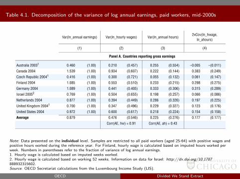
Table 4.1. Decomposition of the variance of log annual earnings, paid workers, mid-2000s
II.4. HOURS WORKED, SELF-EMPLOYMENT AND JOBLESSNESS AS INGREDIENTS OF EARNINGS INEQUALITY
DIVIDED WE STAND: WHY INEQUALITY KEEPS RISING © OECD 2011 177
workers into lower-paid jobs: both developments lead to lower earnings and to higher
earnings inequality. If annual hours worked increase more (or decrease less) among high
wage earners, i.e. wages and hours are correlated positively, changes in hours will also
exacerbate earnings inequality. But if, on the other hand, the annual hours of low-paid
workers rise more, changes in hours will have an equalising effect.18
The following analysis considers changes in both the hourly wage distribution and the
patterns of hours worked across quintiles for the period between the mid-1980s and mid-
2000s. Table 4.A1.2 in Annex 4.A1 shows the components of annual earnings for two
different years in the bottom and top quintiles of the earnings distribution among paid
workers. Columns 1 to 4 report mean weekly hours and mean weeks per year; Columns 5
and 6 display mean annual hours calculated as the product of the first two components;
and Columns 7 and 8 show mean hourly wage rates calculated as total annual wages/
salaries divided by annual hours worked. The main results are summarised in Figure 4.5
Table 4.1. Decomposition of the variance of log annual earnings, paid workers, mid-2000s
Var(ln_annual earnings) Var(ln_hourly wages) Var(ln_annual hours)2xCov(ln_hwage,
ln_ahours)
(1) (2) (3) (4)
Panel A. Countries reporting gross earnings
Australia 20031 0.460 (1.00) 0.210 (0.457) 0.255 (0.554) –0.005 –(0.011)
Canada 2004 1.539 (1.00) 0.934 (0.607) 0.222 (0.144) 0.383 (0.249)
Czech Republic 20041 0.416 (1.00) 0.300 (0.721) 0.055 (0.132) 0.061 (0.147)
Finland 2004 1.085 (1.00) 0.553 (0.510) 0.233 (0.215) 0.298 (0.275)
Germany 2004 1.089 (1.00) 0.441 (0.405) 0.333 (0.306) 0.315 (0.289)
Israel 20052 0.769 (1.00) 0.504 (0.655) 0.198 (0.257) 0.066 (0.086)
Netherlands 2004 0.877 (1.00) 0.394 (0.449) 0.286 (0.326) 0.197 (0.225)
United Kingdom 20041 0.700 (1.00) 0.347 (0.496) 0.229 (0.327) 0.123 (0.176)
United States 2004 0.972 (1.00) 0.600 (0.617) 0.218 (0.224) 0.154 (0.158)
Average 0.879 0.476 (0.546) 0.225 (0.276) 0.177 (0.177)
Corr(AE, hw) = 0.91 Corr(AE, ah) = 0.43
Panel B. Countries reporting net earnings
Austria 2004 0.532 (1.00) 0.386 (0.726) 0.267 (0.502) –0.121 –(0.227)
Belgium 2000 0.358 (1.00) 0.209 (0.584) 0.139 (0.388) 0.010 (0.028)
France 2000 0.654 (1.00) 0.273 (0.417) 0.308 (0.471) 0.073 (0.112)
Greece 2004 0.440 (1.00) 0.318 (0.723) 0.191 (0.434) –0.069 –(0.157)
Hungary 2005 0.498 (1.00) 0.299 (0.600) 0.156 (0.313) 0.043 (0.086)
Ireland 2004 0.604 (1.00) 0.264 (0.437) 0.340 (0.563) 0.000 (0.000)
Italy 2004 0.326 (1.00) 0.238 (0.730) 0.137 (0.420) –0.049 –(0.150)
Luxembourg 2004 0.582 (1.00) 0.330 (0.567) 0.200 (0.344) 0.052 (0.089)
Mexico 20042 0.846 (1.00) 0.813 (0.961) 0.142 (0.168) –0.108 –(0.128)
Spain 2004 0.529 (1.00) 0.280 (0.529) 0.208 (0.393) 0.041 (0.078)
Average 0.537 0.341 (0.627) 0.209 (0.400) –0.013 –(0.027)
Corr(AE, hw) = 0.78 Corr(AE, ah) = 0.31
Note: Samples are restricted to all paid workers (aged 25-64) with positive wages and positive hours worked duringthe reference year. For Finland, hourly wage is calculated based on imputed hours worked per week. Numbers inparentheses refer to the fraction of variance of log annual earnings.1. Hourly wage is calculated based on imputed weeks worked.2. Hourly wage is calculated based on working 52 weeks. Information on data for Israel: http://dx.doi.org/10.1787/
888932315602.Source: OECD Secretariat calculations from the Luxembourg Income Study (LIS).
1 2 http://dx.doi.org/10.1787/888932537731
Note: Data presented on the individual level. Samples are restricted to all paid workers (aged 25-64) with positive wages andpositive hours worked during the reference year. For Finland, hourly wage is calculated based on imputed hours worked perweek. Numbers in parentheses refer to the fraction of variance of log annual earnings.1. Hourly wage is calculated based on imputed weeks worked.2. Hourly wage is calculated based on working 52 weeks. Information on data for Israel: http://dx.doi.org/10.1787888932315602.Source: OECD Secretariat calculations from the Luxembourg Income Study (LIS).
OECD Divided We Stand Extract

Figure 4.5. Changes in annual hours worked and in hourly real wages by earnings quintile,
mid-1980s to mid-2000s
II.4. HOURS WORKED, SELF-EMPLOYMENT AND JOBLESSNESS AS INGREDIENTS OF EARNINGS INEQUALITY
DIVIDED WE STAND: WHY INEQUALITY KEEPS RISING © OECD 2011178
which compares the percentage change in annual hours (left panel) and the change in
hourly real wages (right panel) among workers in the bottom and top quintiles. At first
glance, Figure 4.5 suggests that a decline in low-paid workers’ hours is an important factor
in the rise of inequality in most countries.
Among the countries reporting gross earnings, both changes in hours and hourly wage
rates between higher- and lower-wage earners drove inequality trends. In the Netherlands,
Germany, the Czech Republic, and Canada, the rise in annual earnings inequality among
paid workers was associated with a significant decline in annual hours for the bottom
quintiles, together with an increased dispersion of hourly wages. In Israel and the
Figure 4.5. Changes in annual hours worked and in hourly real wages by earnings quintile, mid-1980s to mid-2000s
Note: Samples are restricted to all paid workers (aged 25-64) with positive wages and positive hours worked during the reference yearwith information on annual hours worked. Mean wages in national currencies at constant 2005 values. Countries ranked in descendingorder of changes in earnings inequality (see Table 4.A1.2).1. Information on data for Israel: http://dx.doi.org/10.1787/888932315602.
Source: OECD Secretariat calculations from the Luxembourg Income Study (LIS).1 2 http://dx.doi.org/10.1787/888932536306
AUS 85-03
FIN 87-04
USA 86-04
CAN 87-04
GBR 86-04
CZE 92-04
ISR 86-051
DEU 84-04
NLD 87-04
HUN 94-05
ESP 95-04
IRL 94-04
FRA 94-00
AUT 94-04
GRC 95-04
BEL 85-00
MEX 84-04
ITA 87-04
LUX 85-04
-30 -20 -10 0 10 20 30%
-40 -20 0 20 40 60 80
-20 0 20 40 60 80
100
-30 -20 -10 0 10 20 30%
-40 100
Panel A. Countries reporting gross earningsChanges in annual hours Changes in hourly wages
Panel B. Countries reporting net earningsChanges in annual hours Changes in hourly wages
Bottom quintile Top quintile
Average
Average
Note: Data presented on the individual level. Samples are restricted to all paid workers (aged 25-64) with positive wages andpositive hours worked during the reference year with information on annual hours worked. Mean wages in national currenciesat constant 2005 values. Countries ranked in descending order of changes in earnings inequality (see Table 4.A1.2).1. Information on data for Israel: http://dx.doi.org/10.1787/888932315602.Source: OECD Secretariat calculations from the Luxembourg Income Study (LIS).
OECD Divided We Stand Extract

Figure 5.1. Inequality (Gini coefficient) of annual earnings among individuals and households, all
working-age households (including individuals and households with no earnings)II.5. TRENDS IN HOUSEHOLD EARNINGS INEQUALITY: THE ROLE OF CHANGING FAMILY FORMATION PRACTICES
DIVIDED WE STAND: WHY INEQUALITY KEEPS RISING © OECD 2011196
Figure 5.1. Inequality (Gini coefficient) of annual earnings among individuals and households, all working-age households (including individuals and households with no earnings)
Note: Samples are restricted to the working-age population (25-64 years) living in a household with a working-age head. Estimatesinclude individuals and households with no earnings. Equivalent household earnings are calculated as the sum of earnings from allhousehold members, corrected for differences in household size with an equivalence scale (square root of household size).1. Information on data for Israel: http://dx.doi.org/10.1787/888932315602.
Source: OECD Secretariat calculations from the Luxembourg Income Study (LIS).1 2 http://dx.doi.org/10.1787/888932536401
Figure 5.2. Inequality (Gini coefficient) of annual earnings among individuals and households, workers and working households
Note: Samples are restricted to the working-age population (25-64 years) living in a household with a working-age head and positiveearnings. Equivalent household earnings are calculated as the sum of earnings from all household members, corrected for differences inhousehold size with an equivalence scale (square root of household size).1. Information on data for Israel: http://dx.doi.org/10.1787/888932315602.
Source: OECD Secretariat calculations from the Luxembourg Income Study (LIS).1 2 http://dx.doi.org/10.1787/888932536420
0.2
0.3
0.4
0.5
0.6
0.7
0.2
0.3
0.4
0.5
0.6
0.7
DNK (2004)
CZE (20
04)
SWE (20
05)
FIN (2
004)
AUS (2003)
NOR (2004)
NLD (2
004)
DEU (2
004)
GBR (2004)
ISR (2005)
1
CAN (2004)
USA (2004)
BEL (2
000)
HUN (2005)
ITA (2
004)
ESP (2
004)
AUT (20
04)
GRC (2004)
FRA (2
000)
IRL (
2004)
LUX (2
004)
POL (20
04)
MEX (2004)
Individual earnings (↗) Household earnings per earner Equivalent household earnings
Countries reporting gross earnings Countries reporting net earnings
Avera
ge
Avera
ge
0.20
0.25
0.30
0.40
0.35
0.45
0.50
0.20
0.25
0.30
0.40
0.35
0.45
0.50
DNK (2004)
CZE (20
04)
SWE (20
05)
FIN (2
004)
AUS (2003)
NOR (2004)
NLD (2
004)
DEU (2
004)
GBR (2004)
ISR (2005)
1
CAN (2004)
USA (2004)
BEL (2
000)
HUN (2005)
ITA (2
004)
ESP (2
004)
AUT (20
04)
GRC (2004)
FRA (2
000)
IRL (
2004)
LUX (2
004)
POL (20
04)
MEX (2004)
Individual earnings (↗) Household earnings per earner Equivalent household earnings
Countries reporting gross earnings Countries reporting net earnings
Avera
ge
Avera
ge
Note: Samples are restricted to the working-age population (25-64 years) living in a household with a working-age head.Estimates include individuals and households with no earnings. Equivalent household earnings are calculated as the sum ofearnings from all household members, corrected for differences in household size with an equivalence scale (square root ofhousehold size).1. Information on data for Israel: http://dx.doi.org/10.1787/888932315602.Source: OECD Secretariat calculations from the Luxembourg Income Study (LIS).
OECD Divided We Stand Extract

Figure 5.2. Inequality (Gini coefficient) of annual earnings among individuals and households,
workers and working households
0.20
0.25
0.30
0.40
0.35
0.45
0.50
0.20
0.25
0.30
0.40
0.35
0.45
0.50
DNK (2004)
CZE (2004)
SWE (2
005)
FIN (2
004)
AUS (2003)
NOR (2004)
NLD (2004)
DEU (2004)
GBR (2004)
ISR (2
005)1
CAN (2004)
USA (2004)
BEL (2000)
HUN (2005)
ITA (2004)
ESP (2004)
AUT (2004)
GRC (2004)
FRA (2000)
IRL (2004)
LUX (2004)
POL (2004)
MEX (2004)
Individual earnings (↗) Household earnings per earner Equivalent household earnings
sgninrae ten gnitroper seirtnuoCsgninrae ssorg gnitroper seirtnuoC
Average
Average
Note: Samples are restricted to the working-age population (25-64 years) living in a household with a working-age head andpositive earnings. Equivalent household earnings are calculated as the sum of earnings from all household members, correctedfor differences in household size with an equivalence scale (square root of household size).1. Information on data for Israel: http://dx.doi.org/10.1787/888932315602.Source: OECD Secretariat calculations from the Luxembourg Income Study (LIS).
OECD Divided We Stand Extract

Figure 5.7. Degree of assortative mating, stricter and broader definitions
II.5. TRENDS IN HOUSEHOLD EARNINGS INEQUALITY: THE ROLE OF CHANGING FAMILY FORMATION PRACTICES
DIVIDED WE STAND: WHY INEQUALITY KEEPS RISING © OECD 2011 203
The OECD average degree of assortative mating, under this broader measure, increases
from 34% to almost 40%.15
Trends in household composition
Another major change that has been happening at the household level and which may
affect inequality is the increase of single-headed (i.e. single-parent, single unattached or
single with unrelated persons) households. Single-headed households are more common
in the Nordic countries and in Canada and the United States where they make up about 25%
Figure 5.7. Degree of assortative mating, stricter and broader definitions
Note: Refers to couple households with both partners working. Earnings refer to net earnings for countries inbrackets and to gross earnings for other countries. 1. Information on data for Israel: http://dx.doi.org/10.1787/888932315602.
Source: OECD Secretariat calculations from the Luxembourg Income Study (LIS).1 2 http://dx.doi.org/10.1787/888932536515
0
2
4
10
6
8
12
14
0
10
20
30
40
60
50
DNK (87-0
4)
SWE (81
-05)
NOR (86-0
4)
FIN (8
7-04)
CZE (92-0
4)
GBR (86-0
4)
CAN (87-0
4)
[AUT (
94-04)]
[HUN (9
4-05)]
[FRA (8
4-00)]
USA (86-0
4)
NLD (8
3-04)
ITA (8
7-04)
[LUX (8
5-04)]
ISR (86-0
5)1
[ESP (9
0-04)]
[GRC (9
5-04)]
[MEX (8
4-04)]
[POL (
92-04)]
AUS (85-0
3)
DEU (8
4-04)
[IRL (
94-04)]
[BEL
(85-0
0)]
DNK (87-0
4)
SWE (81
-05)
NOR (86-0
4)
FIN (8
7-04)
CZE (92-0
4)
GBR (86-0
4)
CAN (87-0
4)
[AUT (
94-04)]
[HUN (9
4-05)]
[FRA (8
4-00)]
USA (86-0
4)
NLD (8
3-04)
[ITA (8
7-04)]
[LUX (8
5-04)]
ISR (86-0
5)1
[ESP (9
0-04)]
[GRC (9
5-04)]
[MEX (8
4-04)]
[POL (
92-04)]
AUS (85-0
3)
DEU (8
4-04)
IRL (
94-04)
[BEL
(85-0
0)]
Panel A. Percentage of workers in earnings decile i with a spouse in the same earnings decile,working couple-households, mid-1980s and mid-2000s
Panel B. Percentage of workers in earnings quintile i with a spouse in the same earnings quintile, working couple households
% of working couples
% of working couples
Early year Recent year (↘)
OECD23
OECD23
Note: Refers to couple households with both partners working. Earnings refer to net earnings for countries in brackets and togross earnings for other countries.1. Information on data for Israel: http://dx.doi.org/10.1787/888932315602.Source: OECD Secretariat calculations from the Luxembourg Income Study (LIS).
OECD Divided We Stand Extract

Figure 9.1. Top 1% income share, 1910-2008
III.9. TRENDS IN TOP INCOMES AND THEIR TAX POLICY IMPLICATIONS
DIVIDED WE STAND: WHY INEQUALITY KEEPS RISING © OECD 2011 347
These data come from the data appendix to Atkinson, Piketty and Saez (2009),1 with
additional information from OECD country delegates in some cases. The information all
comes from tax records, apart from the data for Finland.
Figure 9.1 shows the shares of the top percentile group in pre-tax income for the
English speaking countries from 1910 to 2008 (or the latest available year). The data show
considerable year to year variability, but also shows a clear downward trend in the share for
all six countries, followed by a substantial increase starting in the late1970s or 1980s. In the
case of the United States, the share of the top 1% in 2007 had almost reached the same
levels as before the First World War.
Figure 9.2 shows the top percentile group’s share for France, Germany, Japan, the
Netherlands and Switzerland (Panel A). These countries also show a marked reduction in
the first half of the twentieth century, but there is not the clear increase from the late 1970s
onwards shown by the countries in Figure 9.1. Japan and France both show a slight increase
while the Netherlands and Switzerland show a slight continuing decline and Germany
shows no trend at all.
Figure 9.2, Panel B, shows the top percentile group’s share for Finland, Italy, Norway,
Portugal, Spain and Sweden. Again, there are declines in the first half of the twentieth
century, followed by an increase, with the size of the increase lying somewhere between
the countries in Figure 9.1 and those in Figure 9.2, Panel A. Spain only has data from 1981
and shows a small increase in the top 1% share since then. Denmark is not shown but its
data started in 1990 and show a similar modest increase.
Thus the share of top income recipients in total income in OECD countries was
generally very high before the First World War. There was then a large secular decline in
their share which was particularly sharp during the World War II period. The drop
particularly reflected a decline in capital (rather than labour) incomes. Capital incomes
tended to decline in the inter-war period and then fell sharply during the Second World
War.
Figure 9.1. Top 1% income share, 1910-2008
Source: Alvaredo et al. (2011). Country delegate information: Australia (2000-2008) and Canada (1970-2007).1 2 http://dx.doi.org/10.1787/888932537199
%30
25
20
15
10
5
01910 15 20 25 30 35 40 45 50 55 60 65 70 75 80 85 90 95 2000 05 10
United KingdomNew Zealand United States
CanadaAustralia Ireland
Source: Income refers to individual income. Alvaredo et al. (2011). Country delegate information: Australia (2000-2008) and
Canada (1970-2007).
OECD Divided We Stand Extract

Table 9.1. Share of top 1% in selected years
III.9. TRENDS IN TOP INCOMES AND THEIR TAX POLICY IMPLICATIONS
DIVIDED WE STAND: WHY INEQUALITY KEEPS RISING © OECD 2011 349
The top percentile group experienced a bigger proportionate increase in its share than
the top decile group in the period since 1990 in all countries but Japan – see Figure 9.A2.4 in
Annex 9.A2. This phenomenon was particularly strong in Australia, Canada, the United
Kingdom and the United States, but relatively modest in Belgium, France, the Netherlands,
New Zealand and Switzerland. Within the top percentile group, the top 0.1% has tended to
see the largest (proportionate) increase in their share of total pre-tax incomes. This has
particularly been the case in the United States and, to a lesser degree, Canada and the
United Kingdom as the charts in Annex 9.A2 illustrate – see Figure 9.A2.3 in particular.
In the countries for which data are available, top income shares continued to rise
during the economic expansion to 2007, but then fell back in 2008 with the start of the
financial crisis and drop in stock markets. These developments point up a difficulty in
interpreting data for the 2000s: what movements should be regarded as cyclical and
perhaps therefore temporary? Interpretation of trends can also be clouded by other
temporary factors such as the announcement of a tax reform that affects when income is
declared for tax purposes – see, for instance, the spike for Norway 2004-06.
Further information on changes in income shares of different fractile groups is set out
in the charts in Annex 9.A2. While all the caveats about international comparisons made
above have to be borne in mind, they perhaps apply less strongly to changes in shares. Even
so, changes in tax regimes may affect the measurement of income (as with the “income
shifting” in the United States after the 1986 reforms) differently in different countries. That
said, the scale of the rise in the share of the top 0.1% in the United States stands out as
being substantially larger than the rise in the corresponding share in other countries.
Table 9.1. Share of top 1% in selected years
1970 1980 1990 2000 2001 2002 2003 2004 2005 2006 2007 2008
Australia 5.9 4.8 6.3 7.2 7.6 7.6 7.5 7.7 8.0 8.3 8.9 8.8
Belgium . . 7.0 6.3 7.0 6.7 7.3 7.2 7.6 7.5 7.7 . . . .
Canada 9.0 8.1 9.2 12.4 12.3 12.0 11.9 12.3 12.7 13.3 13.3
Denmark . . 5.2 5.1 6.6 6.3 5.8 6.3 6.6 6.3 7.1 7.4 6.5
Finland 9.9 4.3 4.6 8.8 8.0 7.9 7.9 8.6 . . . . . . . .
France 8.3 7.6 8.2 8.3 8.4 8.5 8.6 8.7 8.7 8.9 . . . .
Germany 11.3 10.8 10.9 11.1 . . . . . . . . . . . . . . . .
Ireland . . 6.7 6.6 10.3 . . . . . . . . . . . . . . . .
Italy . . 6.9 7.8 9.1 9.3 9.3 9.4 9.0 9.1 9.4 9.5 9.4
Japan 8.2 7.2 8.1 8.2 8.5 8.7 8.8 9.0 9.2 . . . . . .
Netherlands 8.6 5.9 5.6 . . . . . . 5.2 5.5 5.6 . . . . . .
New Zealand 6.6 5.7 8.2 8.3 8.8 8.8 9.5 10.0 9.0 . . . . . .
Norway 6.0 4.7 4.4 8.3 7.0 9.4 9.7 10.3 13.8 6.5 7.1 7.5
Portugal . . 4.3 7.2 9.1 9.7 9.0 9.1 9.6 9.8 . . . . . .
Spain . . 7.5 8.4 8.8 8.8 8.5 8.6 8.6 8.8 . . . . . .
Sweden 6.2 4.1 4.4 6.0 6.0 5.7 5.5 5.7 6.3 6.6 6.9 7.1
Switzerland 11.6 8.8 9.7 . . . . . . 9.6 9.9 10.1 10.5 . . . .
United Kingdom 7.1 . . 9.8 12.7 12.7 12.3 12.1 12.9 14.3 . . . . . .
United States 7.8 8.2 13.0 16.5 15.4 14.6 14.9 16.1 17.4 18.0 18.3 17.7
Note: The data in the first four columns relate to the nearest available year.Source: Alvaredo et al. (2011). Country delegate information: Australia (2000-2008), Canada (1970-2007), Italy(2005-2008), Netherlands (2003-2005), Norway (1991-2008) and Switzerland (1970-2006); Roine and Waldenström(2008): Sweden (2007-2008).
1 2 http://dx.doi.org/10.1787/888932538320
Note: The data in the first four columns relate to the nearest available year.Source: Alvaredo et al. (2011). Country delegate information: Australia (2000-2008), Canada (1970-2007), Italy(2005-2008), Netherlands (2003-2005), Norway (1991-2008) and Switzerland (1970-2006); Roine and Waldenstrom (2008):Sweden (2007-2008).
OECD Divided We Stand Extract