Division of Pharmacoepidemiology And Pharmacoeconomics

Technical Report Series

Year: 2013 #007

Metrics for covariate balance in cohort studies of causal effects

Jessica M. Franklina, Jeremy A. Rassena, Diane C. Ackermannb, Dorothee B. Bartelsb,c, Sebastian Schneeweissa

a.) Division of Pharmacoepidemiology and Pharmacoeconomics, Department of Medicine, Brigham and Women’s Hospital and Harvard Medical School, Boston, MA b.) Department of Global Epidemiology, Boerhringer Ingelheim GmbH, Ingelheim, Germany c.) Department of Epidemiology, Hannover Medical School, Hannover, Germany

Series Editors: Sebastian Schneeweiss, MD, ScD Jerry Avorn, MD Robert J. Glynn, ScD, PhD Niteesh K. Choudhry, MD, PhD Jeremy A. Rassen, ScD Josh Gagne, PharmD, ScD Contact Information: Division of Pharmacoepidemiology and Pharmacoeconomics Department of Medicine Brigham and Women’s Hospital and Harvard Medical School 1620 Tremont St., Suite 3030 Boston, MA 02120 Tel: 616-278-0930 Fax: 617-232-8602

1

Metrics for covariate balance in cohort studies of causal effects

Jessica A Myers*1, Jeremy A Rassen1, Diana Ackermann2, Dorothee B Bartels2,3, and Sebastian Schneeweiss1

1 Division of Pharmacoepidemiology and Pharmacoeconomics, Department of Medicine

Brigham and Women’s Hospital and Harvard Medical School, Boston, MA 2 Department of Global Epidemiology, Boehringer Ingelheim GmbH, Ingelheim, Germany

3 Department of Epidemiology, Hannover Medical School, Hannover, Germany

May 21, 2013

Abstract

Inferring causation from non-randomized studies of exposure requires that exposure groups can be

balanced with respect to prognostic factors for the outcome. Although there is broad agreement in

the literature that balance should be checked, there is confusion regarding the appropriate metric.

We present a simulation study that compares several balance metrics with respect to the strength

of their association with bias in estimation of the effect of a binary exposure on a binary, count, or

continuous outcome. The simulations utilize matching on the propensity score with successively

decreasing calipers to produce datasets with varying covariate balance. We propose the novel use

of the C-statistic from the propensity score model estimated in the matched cohort as a balance

metric and found that it had consistently strong associations with estimation bias, even when the

propensity score model was misspecified, as long as the propensity score was estimated with

sufficient study size. This metric, along with the average standardized difference and the general

weighted difference, also introduced in this paper, outperformed all other metrics considered,

including the unstandardized absolute difference, Kolmogorov-Smirnov and Levy distances,

overlapping coefficient, Mahalanobis balance, and L1 metrics. The C-statistic and general weighted

difference also have the advantage that they can evaluate balance on all covariates simultaneously.

Therefore, when combined with the usual practice of comparing covariate means and standard

* Address correspondence to: Dr. Jessica Franklin, 1620 Tremont St., Suite 3030, Boston, MA 02120; email: jmfranklin@partners.org; ph: 617-278-0675.

2

deviations across exposure groups, these metrics may provide useful summaries of the observed

covariate imbalance.

Keywords: bias; confounding factors; covariate balance; matching; propensity score

Financial disclosure: This research was funded by a contract from Boehringer Ingelheim

GmbH to the Brigham and Women’s Hospital.

3

Introduction

Inferring causation from studies of exposure requires that exposure groups can be

balanced with respect to prognostic factors for the outcome. In randomized experiments,

balance is achieved on average for all factors. In nonrandomized studies, prognostic

variables must be measured and balanced via covariate adjustments, such as matching,

stratification, regression, or weighting [1, 2]. Adjustments via a balancing score, such as

the propensity score (PS), can also produce exposure groups that are balanced on

measured predictors of outcome [3, 4]. Although each of these methods are guaranteed to

produce unbiased estimates on average across studies under correctly-specified modeling

assumptions, the bias in any particular study will depend on the balance achieved in that

study, not on expected balance [5].

With cohort study designs, covariate balance can be empirically verified prior to

analyzing outcomes [6]. If exposure groups remain unbalanced after covariate adjustment,

then modifications to the adjustment procedure may produce better balance and improved

estimates of treatment effect. If balance cannot be achieved via any adjustment methods,

then the two populations may not share sufficient overlap to be compared. Poor overlap of

covariates may be likely in the context of newly marketed medications, where patients and

prescribers are often hesitant to initiate the new treatment except as second-line therapy

or for narrowly defined subindications [7]. Investigators may consider postponing safety or

effectiveness comparisons between new and standard treatments until the patient

populations become more similar.

Although there is broad agreement in the literature that balance should be checked

[8, 9], there is confusion in the medical literature regarding an appropriate metric. Initial

4

attempts to characterize covariate imbalance proposed in the context of PS stratification

relied on significance tests for a difference between exposure groups in each covariate [4].

These tests measure the evidence for imbalance in the populations from which study

samples were drawn and are strongly dependent on sample size. More recently, many

investigators rely on examining a simple difference in means with or without

standardization by the covariate standard deviation (SD) [10, 11]. Alternatively, metrics

that characterize balance on the full distribution of individual covariates have been

proposed, including the Kolmogorov-Smirnov distance [12, 13], the Lévy distance [13-15],

and the nonparametric overlapping coefficient [16, 17], also known as the proportion of

similar responses [18]. All of the above metrics measure imbalance on one covariate at a

time. Belitser et al. [19] compared their performance in a simulation study of independent,

normally distributed covariates and concluded that mean differences were superior for

predicting the bias of exposure effect estimates.

A variety of other measures quantify balance on several covariates simultaneously.

The Mahalanobis distance has been extensively discussed in the context of choosing

matches [20-23]. Gu and Rosenbaum [24] proposed a variation on this distance, which

they refer to as Mahalanobis balance, to measure the multivariate distance between

exposure groups, rather than between individuals. Applied studies that utilize PS

adjustment often report the C-statistic of the PS model, which measures the collective

ability of model covariates to discriminate between exposed and unexposed subjects [25].

Austin [26] considered the C-statistic of the PS model as a potential balance diagnostic and

found via simulation that it could not be used to diagnose an incorrect model specification.

However, refitting the PS model after covariate adjustment (for example, after matching)

5

could yield a C-statistic that summarizes the residual imbalance. Finally, Iacus et al. [27]

introduced the L1 balance metric, which measures the proportion of overlap in the exposed

and unexposed multi-dimensional histograms. While L1 has several desirable properties

not available in other balance metrics such as the automatic evaluation of balance in non-

linear and high-order interaction terms, its utility in predicting estimation bias has not

been demonstrated.

The objective of this paper is to compare balance metrics to determine which

metrics are most strongly associated with estimation bias. We present a Monte Carlo

simulation study that evaluates the balance metrics discussed above. We also propose and

evaluate a novel use of the C-statistic to measure covariate balance within a matched

sample as well as a new balance metric, the general weighted difference (GWD). Because

the associations between covariates and outcome determine the amount of bias caused by

a given imbalance, we consider a variety of covariate associations with outcome. We also

expand on past studies [19] by considering a wide spectrum of covariate distributions,

including binomial, multinomial, and skewed, as well as correlated covariates.

Methods

Bias and Balance

Let Xi be the covariate vector for subject i. We assume that this vector includes the

confounders, factors that influence the exposure, Ti, as well as the outcome, Yi. Under a

constant linear exposure effect, a model for the outcome is given by

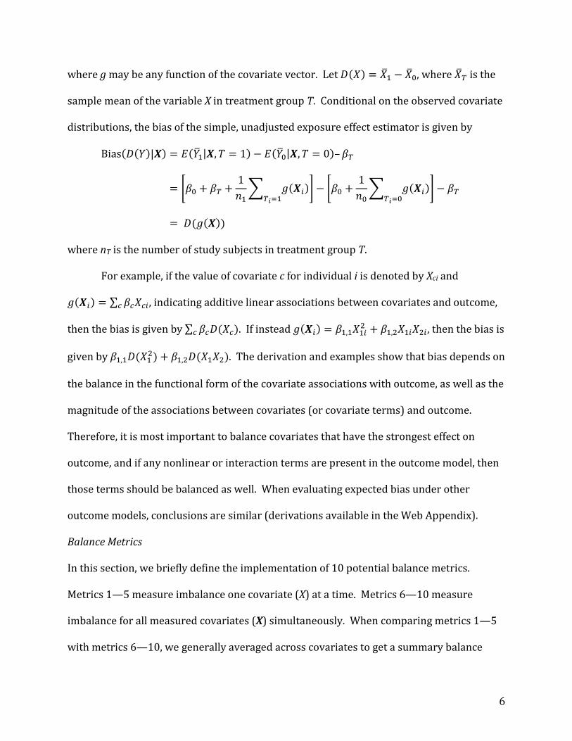
𝐸(𝑌𝑖|𝑿𝒊,𝑇𝑖) = 𝛽0 + 𝛽𝑇𝑇𝑖 + 𝑔(𝑿𝑖)

6

where g may be any function of the covariate vector. Let 𝐷(𝑋) = 𝑋�1 − 𝑋�0, where 𝑋�𝑇 is the

sample mean of the variable X in treatment group T. Conditional on the observed covariate

distributions, the bias of the simple, unadjusted exposure effect estimator is given by

Bias(𝐷(𝑌)|𝑿) = 𝐸(𝑌�1|𝑿,𝑇 = 1) − 𝐸(𝑌�0|𝑿,𝑇 = 0)–𝛽𝑇

= �𝛽0 + 𝛽𝑇 +1𝑛1� 𝑔(𝑿𝑖)

𝑇𝑖=1� − �𝛽0 +

1𝑛0� 𝑔(𝑿𝑖)

𝑇𝑖=0� − 𝛽𝑇

= 𝐷(𝑔(𝑿))

where nT is the number of study subjects in treatment group T.

For example, if the value of covariate c for individual i is denoted by Xci and

𝑔(𝑿𝑖) = ∑ 𝛽𝑐𝑋𝑐𝑖𝑐 , indicating additive linear associations between covariates and outcome,

then the bias is given by ∑ 𝛽𝑐𝐷(𝑋𝑐)𝑐 . If instead 𝑔(𝑿𝑖) = 𝛽1,1𝑋1𝑖2 + 𝛽1,2𝑋1𝑖𝑋2𝑖, then the bias is

given by 𝛽1,1𝐷(𝑋12) + 𝛽1,2𝐷(𝑋1𝑋2). The derivation and examples show that bias depends on

the balance in the functional form of the covariate associations with outcome, as well as the

magnitude of the associations between covariates (or covariate terms) and outcome.

Therefore, it is most important to balance covariates that have the strongest effect on

outcome, and if any nonlinear or interaction terms are present in the outcome model, then

those terms should be balanced as well. When evaluating expected bias under other

outcome models, conclusions are similar (derivations available in the Web Appendix).

Balance Metrics

In this section, we briefly define the implementation of 10 potential balance metrics.

Metrics 1—5 measure imbalance one covariate (X) at a time. Metrics 6—10 measure

imbalance for all measured covariates (X) simultaneously. When comparing metrics 1—5

with metrics 6—10, we generally averaged across covariates to get a summary balance

7

measure; weighted averages, as suggested by Belitser et al. [19], are also possible if

outcome information is available.

Note that each of the balance metrics described below should be estimated in the

sample in which they are meant to describe. For example, to summarize the residual

imbalance that remains after matching, metrics should be calculated in the matched cohort;

in the context of stratification, metrics would be calculated within each stratum; and in the

context of weighting to achieve balance, metrics would be calculated using subject weights

(i.e., the absolute difference would be calculated using the weighted mean in each exposure

group to measure balance in the ‘pseudo-population’). R code for implementation of all

balance metrics is available in Web Appendix 1.

1. The absolute difference is the absolute value of the difference in covariate means

between treatment groups: |𝐷(𝑋)|.

2. The standardized difference is the absolute difference, divided by the pooled within-

group covariate SD: |𝐷(𝑋)|/�(𝑠12 + 𝑠02)/2, where 𝑠𝑇2 is the sample variance of X in

exposure group T.

3. The overlapping coefficient (OVL) is the proportion of overlap in two density

functions, calculated by finding the area under the minimum of both curves:

∫min𝑥�𝑓1(𝑥),𝑓0(𝑥)� 𝑑𝑥, where 𝑓𝑇(𝑥) is the density function in exposure group T

estimated with a normal kernel density estimator and the bandwidth suggested by

Scott [28]. The OVL ranges from 0 to 1 with higher values indicating lower imbalance.

To make it comparable with the other metrics, we generally considered 1-OVL.

8

4. The Kolmogorov-Smirnov (K-S) distance is the maximum vertical distance between

two cumulative distribution functions: max𝑥 |𝐹1� (𝑥) − 𝐹�0(𝑥)|, where 𝐹�𝑇(𝑥) is the

empirical cumulative distribution function in exposure group T.

5. The Lévy distance is the side length of the largest square that can be inscribed between

two cumulative distribution functions:

min𝜖

{𝜖 > 0:𝐹�0(𝑥 − 𝜖) − 𝜖 ≤ 𝐹�1(𝑥) ≤ 𝐹�0(𝑥 + 𝜖) + 𝜖 for all 𝑥}

Both the K-S distance and the Lévy distance range from 0 to 1 with lower values

indicating better balance. See [19] for details on metrics 3—5.

6. The Mahalanobis balance is defined as: (𝑿�1 − 𝑿�0)′Σ−1(𝑿�1 − 𝑿�0), where 𝑿�𝑇 is the

vector of covariate means in exposure group T and Σ is the sample variance-covariance

matrix of covariates. Lower values indicate better balance.

7. The L1 measure requires specification of a stratification for each continuous covariate

(for categorical covariates, the strata are given by the categories). The cross-tabulation

of the covariate-specific strata results in a set of multi-dimensional covariate bins ℋ,

and the L1 measure is calculated as the sum of the imbalances within each bin:

0.5∑ |𝑓1(𝐻)−𝐻∈ℋ 𝑓0(𝐻)|, where 𝑓𝑇(𝐻) is the proportion of subjects in exposure group

T that fall in bin H. This measure varies from 0 to 1 with 0 indicating perfect balance.

When applying the L1 measure, we used the default choice of stratifications as

implemented in the cem package in R [29].

8. The L1 median is a variation on the L1 measure that attempts to weaken its dependence

on a specific stratification. The L1 median is found by first drawing a random sample of

101 multi-dimensional covariate stratifications from the set of all potential

stratifications. The L1 measure is calculated using each of these stratifications in the

9

original (pre-adjustment) cohort, resulting in 101 L1 values. The stratification that

yields the median L1 value (51st out of 101) is used for calculating the L1 median in the

original dataset and all subsequent adjusted datasets (see [27, 29] for details).

9. The C-statistic is the area under the receiver-operating characteristic (ROC) curve from

the PS model. To utilize this statistic as a balance metric, we propose that it be

calculated in the sample that it is meant to describe, as with all other balance metrics.

Therefore, to describe the residual imbalance after PS matching, the C-statistic should

be re-estimated in the matched cohort. The C-statistic ranges from 0.5 to 1.0 with the

minimum indicating that the PS model has no ability to discriminate between treated

and untreated patients, i.e., perfect balance. To compare with other metrics, we

generally considered 𝑐 − 0.5.

10. We also propose the general weighted difference (GWD), given by:

∑ 𝑤𝑎𝑏|𝐷(𝑋𝑎𝑋𝑏)|0≤𝑎≤𝑏≤𝐶 , where C is the number of measured covariates, 𝑋0 is the unit

vector, and 𝑤𝑎𝑏 is a weight assigned to the covariate pair 𝑋𝑎𝑋𝑏. This sum includes the

absolute difference in all individual covariates, all covariate squares, and all pairwise

interactions. Ideally, weights would be based on the strength of association between

covariates (or covariate terms) and outcome, and the empirically derived weights

suggested by Belitser et al. [19] could be extended to develop weights for this purpose.

In the simulations, we assumed that there was no prior knowledge of associations and

that outcome data remained hidden until after matching, as recommended by Rubin

[30]. Thus, as a general-purpose weight, we used 𝑤𝑎𝑏 = 1/𝑠𝑎𝑏 when 𝑎 = 0 and

𝑤𝑎𝑏 = 0.5/𝑠𝑎𝑏 otherwise, giving full weight to differences in individual covariates and

10

half weight to interaction and square terms, standardized by 𝑠𝑎𝑏, the pooled within-

group SD of 𝑋𝑎𝑋𝑏.

Example study

Design and analysis

We implemented the methods described in the previous section in a retrospective cohort

study of the short-term effects of nonsteroidal anti-inflammatory drug (NSAID) use on

gastrointestinal (GI) toxicity and myocardial infarctions (MI) [31-33]. Briefly, our study

population included patients enrolled in Medicare and a state drug insurance program for

the elderly provided by either Pennsylvania or New Jersey. We included all patients 65

years and older that initiated use of a nonselective NSAID (ns-NSAID) or the selective Cox 2

inhibitor, celecoxib, at any point in 1999, the first year that celecoxib was available.

Exposure was classified as ns-NSAID or celecoxib, based on the first prescription.

Covariates were created to capture known risk factors of NSAID-associated gastrotoxicity

and acute MI and were assessed based on healthcare and prescription claims in the 365

days prior to the first NSAID prescription. Beginning on the day after the first NSAID fill,

patients were followed for outcomes until the first of death, loss of Medicare or drug

benefit eligibility, or December 31, 2005.

We evaluated balance before matching by calculating the mean of all covariates in

each treatment group and by calculating the balance summary using each of the 10 metrics

under study. We estimated crude treatment effects for celecoxib versus ns-NSAIDs on GI

and MI events using bivariate Cox proportional hazards models. We then estimated the PS

with a logistic regression including linear terms for all covariates and squared terms for all

11

continuous covariates and performed 1:1 nearest neighbor matching using a caliper of

0.028 (0.2 SDs of the PS), in line with recommendations [34]. We repeated the estimation

of balance and treatment effects within the matched cohort.

Results

Table 1 presents results from the example study. Before matching, strong differences exist

between patients that initiated celecoxib and patients that initiated a ns-NSAID. By far the

largest difference occurs in the proportion of patients with a history of osteoarthritis (51%

of celecoxib users and 33% of ns-NSAID users). Although this difference is large in

magnitude, it is unlikely to be a major source of bias in the analysis since osteoarthritis is

not expected to have a strong association with either outcome. In contrast, the many small

differences that exist in the strongest markers of elevated GI risk (prior GI hemorrhage,

peptic ulcer disease, prior and current use of gastroprotective drugs, and prior use of oral

steroids) and elevated MI risk (coronary artery disease, peripheral vascular disease,

hypertension, congestive heart failure, and prior use of ARBs, beta-blockers, clopidogrel,

and warfarin) may be more concerning, particularly, as all differences are in the same

direction, indicating that celecoxib users are at systematically higher risk of both outcomes.

Many of these differences remain, although reduced, after matching. A small difference in

age (celecoxib users are on average one half year older than ns-NSAID users in the matched

cohort) also remains, further indicating elevated outcome risk in patients using celecoxib.

In evaluating the balance metrics (Table 1), all metrics demonstrate improvement in

balance after matching. While the absolute difference, standardized difference, K-S

distance, and Levy distance differed in absolute value (and are on different scales), they all

indicated approximately a 70% decrease in imbalance through matching. The Mahalanobis

12

metric decreased by 89%, the C-statistic decreased from 0.668 to 0.555 (a 67% reduction

in terms of distance from 0.5), and the GWD decreased by 65%. In contrast, 1-OVL, the L1

measure, and the L1 median decreased by 24%, 0.01%, and 2.4%, respectively.

Many of these metrics align well with the decrease in bias seen in the estimated

effects. The effect on GI events, known from randomized trials to be < 1.0 when comparing

celecoxib to ns-NSAIDs, was reduced from 1.20 to 1.14 after matching, although both

estimates likely suffer from unmeasured confounding [32]. Randomized trials evaluating

the comparative effect on cardiovascular events are ongoing [35], but a review of prior

studies found a rate ratio of 1.06 [36]. In the example study, estimated hazard ratios (HRs)

were reduced from 1.12 to 1.05 through matching.

Simulation Study

Data generation and analysis

We conducted a simulation study to evaluate the association between bias and covariate

imbalance as measured by the ten metrics outlined above. In order to produce datasets

with varying balance and bias, in each simulation scenario we simulated 1000 datasets

with strong imbalance on covariates and then matched each dataset multiple times via 1:1

nearest neighbor matching of exposure groups with successively decreasing calipers of 0.8,

0.4, 0.2, 0.1, and 0.05 SDs of the PS, resulting in a total of 6000 datasets with varying

covariate imbalance.

Datasets were simulated with 6 covariates intended to replicate a wide variety of

realistic measured covariates, shown in Table 1. The first three covariates were

continuous: X1 and X3 were normally distributed, and X2 was a right-skewed lognormal

13

variable. X1 and X2 were on similar scales (X1 had a SD of 1, and X2 was created with a SD of

0.5 on the normal scale, which resulted in a SD of approximately 1 on the lognormal scale),

while X3 was on a much larger scale (SD of 10). Covariates X4 and X5 were binary with

prevalences of 50% and 20%, respectively, and X4 was simulated via a logistic model

conditional on X1 with a log-odds ratio of 2.0 so that X4 was highly correlated with X1 in all

scenarios. Finally, X6 was simulated as an ordered categorical variable with prevalences of

50%, 30%, 10%, 5%, and 5% in categories 1—5, respectively. From these 6 measured

covariates, we created the nonlinear terms, X7= sin(X1) and X8= X22, and the interaction

terms, X9= X3 X4 and X10= X4 X5. The nonlinear terms were intended to provide generic

nonlinear associations with outcome that might be expected when using covariates like

body mass index or seasonality.

Exposure, T, was simulated as a binary variable via the logistic model

logit{Pr(𝑇𝑖 = 1)} = 𝛼𝟎 + 𝜶𝑿𝑖, where Xi is the covariate vector (including squares and

interactions) for subject i and α = (α1, …, α10). The parameters in α define the log odds

ratios between covariates and exposure in the pre-matched dataset, and higher absolute

values generally indicate more imbalance. In the primary simulation scenarios, the

outcome, Y, was simulated as a binary variable via the logistic model logit{Pr(𝑌𝑖 = 1)} =

𝛽𝟎 + 𝜷𝑿𝒊 + 𝛽𝑇𝑇𝑖, where β = (β1, …, β10). Additional simulation scenarios considered

continuous outcomes generated via a linear model and Poisson event counts generated via

a log-linear model (described in detail in the Web Appendix). The β parameters define the

association between covariates and outcome as log-odds ratios, and 𝑒𝛽𝑇 is the true causal

effect of exposure on outcome, expressed as an odds ratio.

14

In each dataset, we estimated two PS models via logistic regression. In the first

model (PS1), we include terms X1—X6 only (no nonlinear or interaction terms). We may

think of this as the “usual practice” setting, where investigators include only main effects of

covariates in the PS model. In the second model (PS2), we include all covariate terms X1—

X10. We may think of this as the “special knowledge” setting, where investigators have

some additional knowledge that these particular nonlinear terms and interactions are

important to balance. Matching was carried out using each of the two estimated PSs.

We measured covariate balance using each potential metric before and after each

round of matching. For metrics that measure balance only one covariate at a time, we

applied the metric to each measured covariate X1—X6, and then took the average across

covariates. For calculating the C-statistic, the PS that was used for matching was re-

estimated in the matched data in order to measure the ability of covariates to discriminate

between treated and untreated patients after matching (i.e., to measure balance in the

matched sample). Bias was also calculated before and after each round of matching as the

difference between the estimated crude odds ratio and the true exposure odds ratio, 𝑒𝛽𝑇 .

To measure the association between each balance metric and bias, we estimated a

separate linear model for each balance metric that included bias as the dependent variable

and linear and squared terms for balance as independent variables. From these models, we

extracted the proportion of variation explained (R2) to measure the strength of the

association. We also extracted the estimated intercept from each model as a measure of

the absolute magnitude of bias relative to measured imbalance; an intercept of 0 is

preferred, indicating that bias and imbalance approach 0 simultaneously. We do not

present the linear correlations between bias and balance, as done in other simulation

15

studies [19], as we have found that the relative linearity of the association between bias

and balance tends to depend on the region of bias that is explored. Furthermore, we

generally focus on the relative R2 across metrics within the simulation scenario, since the

magnitude of the R2 in a given scenario depends strongly on the proportion of variation

explained in the outcome-generating model. When the cumulative strength of association

between covariates and outcome is weaker, the R2 measuring the association between bias

and balance will also be weaker across all metrics.

Simulation scenarios

We simulated data under 7 sets of values for the sample size, N, and the α and β

parameters, as shown in Table 1. In order to avoid issues of ‘non-collapsibility’ of the odds

ratio [37], we used 𝛽𝑇 = 0, indicating no effect in all simulation scenarios. In all but one

scenario, we used a sample size of N=5000 and chose values for 𝛼𝟎 and 𝛽𝟎 so that the

overall prevalence of exposure is approximately 50% and the overall outcome rate is

approximately 5%. The other parameter values were chosen to create initial datasets with

high imbalance on covariates and relatively strong confounding.

In the base case, neither of the outcome or exposure-generating models contained

any nonlinear or interaction covariate terms, X7—X10. The “base case” was repeated using a

lower exposure prevalence of approximately 20% (the “low exposure prevalence” case)

and using a smaller sample size of N=500 (the “small sample” case). In the “nonlinear

outcome” scenario, nonlinear and interaction terms were present in the outcome-

generating model, and in the “nonlinear outcome and exposure” case, these terms were

present in both outcome and exposure-generating models. In the “redundant covariates”

case, the covariates X1 and X4 were redundant in the sense that they were highly correlated

16

(as in all simulation scenarios), but only X1 had a direct effect on exposure or outcome. This

scenario was designed to understand the benefits of the Mahalanobis balance, which

utilizes the covariance among variables to avoid over-penalizing imbalance on multiple

covariates that are highly correlated.

The “instrumental variables” case evaluated the performance of balance metrics

when there are instrumental variables (IVs) present in the set of covariates to be balanced.

An IV (also known as an instrument) is a variable that influences exposure but has no

impact on outcome except through its association with exposure. We specified X2 to be an

instrument by setting the coefficients to zero on all terms in the outcome-generating model

involving X2. Past work has shown that balancing instruments can increase bias from

residual confounding [38, 39]. Since all of the balance metrics considered do not

incorporate information on covariate associations with outcome, we expected that all

metrics would perform poorly in this case.

Results

Figure 1 presents the PS distributions for one example dataset from the base case scenario.

As expected, in this case PS1 and PS2 provided almost identical distributions. On both PSs,

the unmatched data were highly imbalanced in the PS. As matching was performed with

increasingly tight calipers, balance on the PS improved incrementally, and it was nearly

perfect when using the smallest caliper. Results for all other simulation scenarios were

very similar to those presented for the base case.

Also for the base case, Figure 2 presents the mean bias on the x-axis versus the

mean imbalance as measured by each of the ten metrics on the y-axis. Means are taken

across the 1000 datasets in each round of matching, so that the right-most point in each

17

plot shows the average bias and balance in the generated datasets before matching, and the

point nearest to the origin (0,0) shows the average bias and balance for the 1000 datasets

created by matching with the tightest caliper. Bias and imbalance are both shown with

95% quantile bars to show the variation across datasets in each round of matching.

Nearly all of the ten imbalance measures were strongly associated with bias. In

particular, when matching on the correctly specified PS (PS1) both the GWD and the

standardized difference explained 89.2% of the variation in bias. The similarity between

these two measures was expected in this case, since there was no structural imbalance on

nonlinear and interaction terms. The C-statistic, the K-S distance, and the Lévy distance

were also associated with estimation bias, explaining 89.1% of the variation, but the

intercept for the C-statistic was much smaller than for the latter metrics, indicating better

correspondence between the C-statistic and bias. By contrast, both the L1 measure and the

L1 median were poor predictors of bias. In datasets matched with a caliper of 0.05 SDs of

PS1, bias was approximately zero, but the L1 measure with the default bin choice was on

average 0.9, indicating almost perfect separation. In addition, the Mahalanobis balance

indicated nearly perfect balance after matching with a caliper of 0.2 SDs of PS, even though

the average bias was relatively strong in that case. These issues are reflected in the

estimated intercepts far from 0.

Figure 2 also shows that the variation in effect estimates decreased as we matched

with successively smaller calipers, even though the sample size also decreased. This

phenomenon is due to the fact that increasing balance on prognostic covariates reduced the

variation in outcomes, which resulted in improved efficiency of effect estimates.

18

Figures showing the results of all simulation scenarios, as in Figure 2, are available

in the Web Appendix. Figure 3 summarizes these results. The top panel in Figure 3

presents the estimated intercept for each balance metric and the 5 main simulation

scenarios. The bottom panel presents the variation explained (R2) for each metric as

compared to that of the GWD. This figure shows that many of the balance metrics perform

similarly, but some perform better across simulation scenarios. Specifically, the

standardized difference, the C-statistic, and the GWD nearly always have the highest R2,

indicating strong associations with bias. In addition, these metrics have estimated

intercepts near 0, indicating that they accurately identify the zero-bias scenario. The K-S

distance and the Lévy distance generally have high R2 values, but tend to over-estimate

imbalance when there is 0 bias. The absolute difference was also often strongly associated

with bias, but this association was inconsistent across simulation scenarios and PS models.

The absolute difference, the OVL, and the Mahalanobis balance had consistently weaker

associations with bias than most other metrics, even in the “redundant covariates”

scenario, which was specifically designed to expose the strengths of the Mahalanobis

balance. The L1 measure and L1 median had the weakest associations with bias across all

simulation scenarios, and the results for the L1 measure are not shown, as its values were

outside the plotting range in all plots.

The scenarios not shown in Figure 3, which repeated the base case with a smaller

study size or lower exposure prevalence, had similar results to the scenarios shown, with a

few exceptions. Specifically, both of these scenarios resulted in lower performance for the

C-statistic, due to the small number of exposed patients and imprecise estimation of the PS,

and, thus, the C-statistic. However, performance was still comparable to other measures;

19

for example, in the low study size scenario, the C-statistic explained 72.1% of the variation

in bias, versus 72.2% explained by the best metrics in this scenario (the GWD, Mahalanobis

balance, and standardized difference). Complete results for these scenarios are also

available in the Web Appendix. Finally, results for simulations using other outcome types

(Poisson and continuous) were very similar to the results presented here and are available

in the Web Appendix.

Discussion

In this paper, we evaluated ten potential measures of imbalance with respect to their

correlation with estimation bias, including a new GWD measure and a novel use of the C-

statistic for measuring balance. We found that several measures were consistently good

predictors of bias, but the standardized difference, the C-statistic, and the GWD provided

the best performance. Based on these results, we recommend these measures for use in

measuring covariate imbalance in cohort studies. The GWD may be preferred when an

investigator has some additional knowledge of which covariates are the strongest

predictors of outcome, and thus, most important to balance, because this knowledge can be

incorporated into the specification of weights. The average standardized difference could

similarly be weighted across covariates, using the suggestions of Belitser et al., but these

weightings were not evaluated in this study. When information on outcome associations is

not available, the C-statistic may be preferred. Although the C-statistic depends on the

specification of the PS model, this metric performed well in the simulation studies even

when based on an under-specified PS (that was missing nonlinear and interaction terms)

20

or an over-specified PS (such as PS2 in the “instrumental variables” scenario). In addition,

the C-statistic has a finite scale that is already familiar to most investigators.

The simulation study also showed that the Mahalanobis balance was generally

highly correlated with bias, but it was nonetheless consistently outperformed by other

measures, even in the scenario specifically designed to demonstrate its strengths.

Furthermore, the L1 measures had consistently weaker associations with estimation bias

than all other metrics, indicating that the default stratification choices as implemented by

these measures do not necessarily perform well.

Although the relative performance of the various metrics was generally consistent

across the simulation scenarios considered, the specific results observed are dependent on

the data-generating process and parameter values chosen. Specifically, the good

performance of the standardized difference across scenarios is likely due, in part, to the

relatively weak effects on outcome for the nonlinear and interaction terms that were

simulated. While we attempted to choose effect sizes that would produce reasonable

outcome models, data generated with stronger effects of nonlinear or interaction terms

would probably reduce the association between the standardized difference and bias, since

this measure does not account for imbalance in these factors. Similarly, although the C-

statistic performed well in the case of a misspecified PS model, this metric is certain to

perform better when the PS is correctly specified with all covariates and covariate terms

affecting outcome; it is similarly certain to perform worse in the case of severe

misspecification. The success of the default weighting scheme in the GWD metric is also

likely somewhat subject to the simulation scenarios chosen, as many highly correlated

covariates may induce very large values of GWD that do not appropriately reflect likely

21

bias. However, across dozens of simulation scenarios examined (including scenarios not

presented in this paper), the performance of the default GWD weighting was surprisingly

robust.

Most importantly, we have assumed throughout that investigators have identified a

set of covariates that are related to outcome and need to be balanced. Prior work has

shown that balancing some covariates, including mediators (variables on the causal

pathway from exposure to outcome) and IVs of the exposure-outcome relationship, can

increase, rather than decrease, bias from unobserved confounders [38-43]. The

performance of all metrics may be worse if these variables are included in the list of

covariates to be balanced or if important confounders are omitted.

Finally, in this paper we focused on a single overall measure of the imbalance across

covariates. A single metric may be simpler to evaluate and may be particularly useful in

genetic matching, where matching is based on minimizing a loss function for covariate

imbalance [44]. However, the results of this study should not discourage investigators

from the common practice of evaluating balance one covariate at a time. Evaluating the

difference between exposure groups in the mean and SD of an individual covariate can

provide an assessment of balance on the scale of the covariate that can then be directly

interpreted by investigators as to its potential for confounding. In addition, examining

these differences across covariates, as in a forest plot [26], can identify whether the

imbalances are random or if they are clustered in a set of related covariates and represent

real uncontrolled confounding.

22

References

1. Billewicz W. The efficiency of matched samples: An empirical investigation. Biometrics 1965; 21: 623-644. 2. Cochran WG. The effectiveness of adjustment by subclassification in removing bias in observational studies. Biometrics 1968; 24: 295-313. 3. Rosenbaum PR, Rubin DB. The central role of the propensity score in observational studies for causal effects. Biometrika 1983; 70: 41-55. 4. Rosenbaum PR, Rubin DB. Reducing bias in observational studies using subclassification on the propensity score. Journal of the American Statistical Association 1984; 79: 516-524. 5. Hirano K, Imbens GW, Ridder G. Efficient estimation of average treatment effects using the estimated propensity score. Econometrica 2003; 71: 1161-1189. 6. Schneeweiss S, Avorn J. A review of uses of health care utilization databases for epidemiologic research on therapeutics. Journal of clinical epidemiology 2005; 58: 323-337. 7. Seeger JD, Williams PL, Walker AM. An application of propensity score matching using claims data. Pharmacoepidemiology and drug safety 2005; 14: 465-476. 8. Rubin DB. On principles for modeling propensity scores in medical research. Pharmacoepidemiology and drug safety 2004; 13: 855-857. 9. Ho DE, Imai K, King G, Stuart EA. Matching as nonparametric preprocessing for reducing model dependence in parametric causal inference. Political Analysis 2007; 15: 199-236. 10. Austin PC. Assessing balance in measured baseline covariates when using many-to-one matching on the propensity-score. Pharmacoepidemiology and drug safety 2008; 17: 1218-1225. 11. Austin PC. Goodness-of-fit diagnostics for the propensity score model when estimating treatment effects using covariate adjustment with the propensity score. Pharmacoepidemiology and drug safety 2008; 17: 1202-1217. 12. Stephens MA. Use of the Kolmogorov-Smirnov, Cramer-Von Mises and related statistics without extensive tables. Journal of the Royal Statistical Society, Series B 1970; 32: 115-122. 13. Pestman WR. Mathematical statistics: An introduction. Walter De Gruyter Inc: Berlin, 1998. 14. Lévy P. Théorie de l'addition des variables aléatoires. Gauthier-Villars, 1937. 15. Zolotarev VM. Estimates of the difference between distributions in the Lévy metric. Trudy Matematicheskogo Instituta im. VA Steklova 1971; 112: 224-231. 16. Bradley E. Overlapping coefficient. Encyclopedia of Statistical Sciences 1985; 6: 546-547. 17. Inman HF, Bradley EL. The overlapping coefficient as a measure of agreement between probability distributions and point estimation of the overlap of two normal densities. Communications in Statistics-Theory and Methods 1989; 18: 3851-3874. 18. Rom DM, Hwang E. Testing for individual and population equivalence based on the proportion of similar responses. Statistics in medicine 1996; 15: 1489-1505.

23

19. Belitser SV, Martens EP, Pestman WR, Groenwold RHH, Boer A, Klungel OH. Measuring balance and model selection in propensity score methods. Pharmacoepidemiology and drug safety 2011. 20. Cochran WG, Rubin DB. Controlling bias in observational studies: A review. Sankhyā: The Indian Journal of Statistics, Series A 1973; 35: 417-446. 21. Rubin DB. Bias reduction using Mahalanobis-metric matching. Biometrics 1980; 36: 293-298. 22. Rubin DB. Multivariate matching methods that are equal percent bias reducing, I: Some examples. Biometrics 1976; 32: 109-120. 23. Rubin DB. Using multivariate matched sampling and regression adjustment to control bias in observational studies. Journal of the American Statistical Association 1979; 74: 318-328. 24. Gu XS, Rosenbaum PR. Comparison of multivariate matching methods: Structures, distances, and algorithms. Journal of Computational and Graphical Statistics 1993; 2: 405-420. 25. Stürmer T, Joshi M, Glynn RJ, Avorn J, Rothman KJ, Schneeweiss S. A review of the application of propensity score methods yielded increasing use, advantages in specific settings, but not substantially different estimates compared with conventional multivariable methods. Journal of clinical epidemiology 2006; 59: 437. e431-437. e424. 26. Austin PC. Balance diagnostics for comparing the distribution of baseline covariates between treatment groups in propensity-score matched samples. Statistics in medicine 2009; 28: 3083-3107. 27. Iacus SM, King G, Porro G. Multivariate matching methods that are monotonic imbalance bounding. Journal of the American Statistical Association 2011; 106: 345-361. 28. Scott DW. Multivariate density estimation. Wiley Online Library, 1992. 29. Iacus SM, King G, Porro G. CEM: Coarsened exact matching software. Journal of statistical Software 2009; 30: 1-27. 30. Rubin DB. The design versus the analysis of observational studies for causal effects: parallels with the design of randomized trials. Statistics in medicine 2007; 26: 20-36. 31. Brookhart MA, Wang P, Solomon DH, Schneeweiss S. Evaluating short-term drug effects using a physician-specific prescribing preference as an instrumental variable. Epidemiology 2006; 17: 268-275. 32. Schneeweiss S, Glynn RJ, Tsai EH, Avorn J, Solomon DH. Adjusting for unmeasured confounders in pharmacoepidemiologic claims data using external information: the example of COX2 inhibitors and myocardial infarction. Epidemiology 2005; 16: 17-24. 33. Schneeweiss S, Solomon DH, Wang PS, Rassen J, Brookhart MA. Simultaneous assessment of short-term gastrointestinal benefits and cardiovascular risks of selective cyclooxygenase 2 inhibitors and nonselective nonsteroidal antiinflammatory drugs: an instrumental variable analysis. Arthritis & Rheumatism 2006; 54: 3390-3398. 34. Austin PC. Optimal caliper widths for propensity-score matching when estimating differences in means and differences in proportions in observational studies. Pharmaceutical Statistics 2011; 10: 150-161. 35. MacDonald TM, Mackenzie IS, Wei L, Hawkey CJ, Ford I, Hallas J, Webster J, Reid D, Ralston S, Walters M. Methodology of a large prospective, randomised, open, blinded endpoint streamlined safety study of celecoxib versus traditional non-steroidal anti-

24

inflammatory drugs in patients with osteoarthritis or rheumatoid arthritis: protocol of the standard care versus celecoxib outcome trial (SCOT). BMJ open 2013; 3. 36. White WB, Faich G, Borer JS, Makuch RW. Cardiovascular thrombotic events in arthritis trials of the cyclooxygenase-2 inhibitor celecoxib. The American journal of cardiology 2003; 92: 411. 37. Miettinen OS, Cook EF. Confounding: Essence and detection. American journal of epidemiology 1981; 114: 593-603. 38. Myers JA, Rassen JA, Gagne JJ, Huybrechts KF, Schneeweiss S, Rothman KJ, Joffe MM, Glynn RJ. Effects of adjusting for instrumental variables on bias and precision of effect estimates. American journal of epidemiology 2011; 174: 1213-1222. 39. Pearl J. On a class of bias-amplifying variables that endanger effect estimates. In On a class of bias-amplifying variables that endanger effect estimates, Editor (ed)^(eds). AUAI: City, 2010. 40. Greenland S. Quantifying biases in causal models: classical confounding vs collider-stratification bias. Epidemiology 2003; 14: 300--306. 41. Pearl J. Causality: models, reasoning, and inference. Cambridge Univ Press, 2000. 42. Schisterman EF, Cole SR, Platt RW. Overadjustment bias and unnecessary adjustment in epidemiologic studies. Epidemiology 2009; 20: 488--495. 43. Brookhart MA, Schneeweiss S, Rothman KJ, Glynn RJ, Avorn J, Stürmer T. Variable selection for propensity score models. American journal of epidemiology 2006; 163: 1149-1156. 44. Diamond A, Sekhon JS. Genetic Matching for Estimating Causal Effects: A General Multivariate Matching Method for Achieving Balance in Observational Studies. In Genetic Matching for Estimating Causal Effects: A General Multivariate Matching Method for Achieving Balance in Observational Studies, Editor (ed)^(eds). City, 2010.

25

Table 1. Covariate balance and treatment effect estimates in the example study. Matching was performed with a caliper of 0.028 (0.2 SDs of the PS).

Before matching After matching Celecoxib ns-NSAID Celecoxib ns-NSAID N 8,354 6,430 5,911 5,911 Demographics: mean (sd) / proportion Age 79.9 (6.9) 78.2 (7.0) 79.1 (6.8) 78.6 (6.9) Female 0.85 0.78 0.82 0.81 Black race 0.09 0.13 0.10 0.11 Other race 0.03 0.04 0.03 0.03 Comorbidities: proportion Coronary artery disease 0.48 0.43 0.45 0.43 Prior GI hemorrhage 0.07 0.05 0.06 0.05 Peptic ulcer disease 0.23 0.16 0.19 0.17 Peripheral vascular disease 0.21 0.17 0.19 0.18 Osteoarthritis 0.51 0.33 0.41 0.35 Rheumatoid arthritis 0.08 0.04 0.05 0.04 Diabetes mellitus 0.31 0.31 0.31 0.31 Hyperlipidemia 0.53 0.50 0.51 0.51 Transient ischemic attack 0.07 0.06 0.06 0.06 Stroke 0.10 0.09 0.09 0.09 Angina 0.09 0.09 0.09 0.09 New MI 0.04 0.04 0.04 0.04 Old MI 0.05 0.05 0.05 0.05 Hypertension 0.80 0.78 0.79 0.78 Congestive heart failure 0.26 0.21 0.23 0.22 COPD 0.24 0.22 0.23 0.22 Chronic kidney disease 0.06 0.05 0.06 0.05 Medications: proportion ACE inhibitors 0.27 0.27 0.27 0.27 ARBs 0.09 0.07 0.08 0.07 Beta blockers 0.34 0.32 0.33 0.33 Clopidogrel 0.06 0.04 0.06 0.05 Oral steroids 0.14 0.11 0.13 0.11 Diabetes drugs 0.17 0.19 0.18 0.19 Gastroprotective drugs 0.41 0.30 0.35 0.32 Other lipid lowering drugs 0.02 0.02 0.02 0.02 Statins 0.25 0.25 0.25 0.25 Warfarin 0.12 0.06 0.08 0.07 Concurrent gastroprotective drugs 0.25 0.17 0.20 0.18 Health services intensity: mean (sd) Number of prior hospitalizations 0.54 (1.1) 0.48 (1.0) 0.50 (1.1) 0.48 (1.0) Number of days hospitalized 4.4 (11.1) 3.9 (10.3) 4.0 (10.7) 3.8 (10.0) Number of distinct generics 11.6 (6.1) 10.5 (5.6) 11.0 (5.8) 10.7 (5.7) Number of days in a nursing home 1.77 (8.7) 1.43 (8.4) 1.56 (8.4) 1.44 (8.2) Combined comorbidity score 1.76 (2.4) 1.52 (2.4) 1.60 (2.4) 1.54 (2.4) Number of doctor visits 11.2 (7.6) 10.1 (7.9) 10.7 (7.4) 10.3 (7.9) Balance metrics Absolute difference 0.160 0.049

26

Standardized difference 0.095 0.028 1 – OVL 0.065 0.049 Kolomogrov-Smirnov distance 0.038 0.012 Levy distance 0.036 0.010 Mahalanobis balance 0.339 0.038 C-statistic – 0.5 0.168 0.055 L1 measure 1.000 0.999 L1 median 0.851 0.830 Generalized weighted difference 0.036 0.012 Estimated treatment effects: HR (95% CI) GI events 1.20 (1.01—1.41) 1.14 (0.95—1.37) MI events 1.12 (1.00—1.25) 1.05 (0.93—1.18) Table 2. Covariate terms and parameters for simulation studies. The variable column gives the mean and SD (on the normal distribution scale) for the continuous covariates and the prevalence for the binary covariates. The α values determine the association between covariates and exposure as log odds ratios. The β values determine the association between covariates and outcome as log odds ratios.

Variable Base case Nonlinear

outcome

Nonlinear outcome and

exposure

Redundant covariates

Instrumental variables

Low exposure

prevalence

Small study size

N=5000 N=5000 N=5000 N=5000 N=5000 N=5000 N=500 α β α β α β α β α β α β α β

Intercept -3.5 -5 -3.5 -3.5 -1 -3.5 -1.3 -3.7 -1.3 -3.7 -5 -3.3 -3.5 -3.3 X1 Normal (0,1) 1.0 0.5 1.0 0.4 0.8 0.4 0.8 0.4 0.8 0.4 1.0 0.5 1.0 0.5 X2 Lognormal (0,0.5) 1.0 0.5 1.0 0.03 0.06 0.03 0.06 0.03 0.06 0 1.0 0.5 1.0 0.5 X3 Normal (0,10) 0.1 0.05 0.1 0.03 0.06 0.03 0.1 0.05 0.06 0.03 0.1 0.05 0.1 0.05 X4 Binary (p=0.5) 2.0 1.0 2.0 0.75 1.5 0.75 0 0 1.5 0.75 2.0 1.0 2.0 1.0 X5 Binary (p=0.2) 2.0 1.0 2.0 0.75 1.5 0.75 2.0 1.0 1.5 0.75 2.0 1.0 2.0 1.0 X6 Ordinal categorical 0.4 0.2 0.4 0.2 0.4 0.2 0.4 0.3 0.4 0.2 0.4 0.2 0.4 0.2 X7 sin(X1) 0 0 0 0.4 0.8 0.4 0.8 0.4 0.8 0.4 0 0 0 0 X8 X22 0 0 0 0.02 0.04 0.02 0.04 0.02 0.04 0 0 0 0 0 X9 X3 X4 0 0 0 0.04 0.08 0.04 0 0 0.08 0.04 0 0 0 0 X10 X4 X5 0 0 0 0.5 1.0 0.5 0 0 1.0 0.5 0 0 0 0

27

Figure 1: One example dataset from the base case simulation scenario before and after matching on PS1 (left) or PS2† (right). The PS distribution in exposed patients (dashed curve) and unexposed patients (solid curve) in the unmatched data is in the top panel and lower panels are after matching with calipers of 0.8, 0.4, 0.2, 0.1, and 0.05 SDs of the PS (in order from top to bottom). The average number of treated patients across simulations in each sample is shown in the upper left corner.

† PS1 is the estimated PS that includes covariate terms X1—X6 only. PS2 is the estimated PS that includes covariate terms X1—X10.

28

Figure 2: Base Case. Mean and 95% quantile bars for bias (x-axis) and covariate imbalance (y-axis). Means are taken across 1000 simulated datasets in unmatched data (right-most point) and each matched dataset (moving left as the caliper decreases). Datasets were matched on PS1 (left) and on PS2 (right), and the intercept (�̂�0) and variation explained (R2) are in the lower right corner.

29

Figure 3: Results from 5 main simulations scenarios. The intercept from each metric is plotted in the top panel, and the ratio comparing the variation in bias explained by each balance metric versus the variation explained by the GWD is plotted in the bottom panel. The left and right panels show results when matching on PS1 and PS2, respectively. The x-axis in each plot is the simulation scenario. Results for the L1 measure are not shown because they are outside of the plotting region for all scenarios.