dmrb air quality model verification - highways...
TRANSCRIPT

Highways Agency
DMRB Air Quality Model Verification
Good Practice Guide
210664.26
Issue | March 2011
This report takes into account the particular
instructions and requirements of our client.
It is not intended for and should not be relied
upon by any third party and no responsibility is
undertaken to any third party.
Job number 210664.26
Ove Arup & Partners Ltd
13 Fitzroy Street
London
W1T 4BQ
United Kingdom
www.arup.com

210664.26 | Issue | 17 March 2011
J:\210000\210664-26 HA MODEL VERIFICATION STUDY\4 INTERNAL PROJECT DATA\4-05 ARUP REPORTS\0007REPORT ISSUE.DOCX
Document Verification
Job title DMRB Air Quality Model Verification Job number
210664.26
Document title Good Practice Guide File reference
Document ref 210664.26
Revision Date Filename 0001Report Draft 1.docx
Draft 1 22/11/10 Description First draft
Prepared by Checked by Approved by
Name Michael Bull Carl Hawkings Michael Bull
Signature
Draft 2 01/03/11 Filename 0004Report Draft to Client.docx Description Amended with Client Comments
Prepared by Checked by Approved by
Name Michael Bull Carl Hawkings Michael Bull
Signature
Issue 17/03/11 Filename 0007Report Issue.docx Description
Prepared by Checked by Approved by
Name Michael Bull Carl Hawkings Michael Bull
Signature
Filename Description
Prepared by Checked by Approved by
Name
Signature
Issue Document Verification with Document

Highways Agency DMRB Air Quality Model Verification Good Practice Guide
210664.26 | Issue | 17 March 2011
J:\210000\210664-26 HA MODEL VERIFICATION STUDY\4 INTERNAL PROJECT DATA\4-05 ARUP REPORTS\0007REPORT ISSUE.DOCX
Contents
Page
1 Introduction 1
2 Why Verify Dispersion Models 2
3 Factors Affecting Air Quality Assessments 4
3.1 Traffic Data and Vehicle Emission Factors 4
3.2 NOx:NO2 Conversion 7
3.3 Types of Monitoring 8
3.4 Local Site Characteristics 9
3.5 Projecting Forward 10
3.6 Matching Verification Period with Traffic Modelling Data/Time of Day 10
3.7 Background Concentrations 13
3.8 Drop Off Rates from the Road 14
3.9 Identifying Verification Zones 16
4 Identifying Approaches to Model Verification 17
4.1 Review of Current Approaches 17
4.2 Potential Issues with TG09 Approach of HA Studies 18
4.3 Review of Published Model Validation Studies 22
4.4 Performance of Models in the UK 28
4.5 Pollutants to be Used in Verification 30
5 Recommendations for Verification Approach 32
5.1 Overall Approach for Verification 32
5.2 Model Verification Approach with Annual Mean Data 32
5.3 Model Verification Approach where Continuous Monitoring Data are Available 34
5.4 Acceptable Limits for Model Adjustment 37
Appendices
Appendix A
Model Verification Check List

Highways Agency DMRB Air Quality Model Verification Good Practice Guide
210664.26 | Issue | 17 March 2011
J:\210000\210664-26 HA MODEL VERIFICATION STUDY\4 INTERNAL PROJECT DATA\4-05 ARUP REPORTS\0007REPORT ISSUE.DOCX Page 1
1 Introduction
Ove Arup and Partners Ltd (Arup) of the Seligere consortium, has been commissioned by the Highways Agency (HA) to prepare a good practice guide on air quality model verification for large scale transport schemes. The scope of the study is to:
Develop a preferred approach to model verification for HA schemes;
Obtain comments and views from the air quality community on model verification and seek peer review on the recommended approach; and
To produce a Good Practice Guide on air quality model verification for HA schemes.
This report presents the results of this study and provides a draft Good Practice Guide.
Throughout this report the following terms are used in the same manner as defined in Annex 3 of the DEFRA Technical Guidance Document LAQM.TG09
1:
Model Validation: refers to the general comparison of modelled results against modelled data carried out by model developers.
Model Verification: is the process by which modelling and input data uncertainties are investigated and where possible minimised.
Model Adjustment: Is the adjustment of model results to ensure final concentrations are representative of the monitoring information from an area.
1 Local Air Quality Management, Technical Guidance LAQM.TG(09), DEFRA, February 2009
Highways Agency DMRB Air Quality Model Verification Good Practice Guide
210664.26 | Issue | 17 March 2011
J:\210000\210664-26 HA MODEL VERIFICATION STUDY\4 INTERNAL PROJECT DATA\4-05 ARUP REPORTS\0007REPORT ISSUE.DOCX Page 2
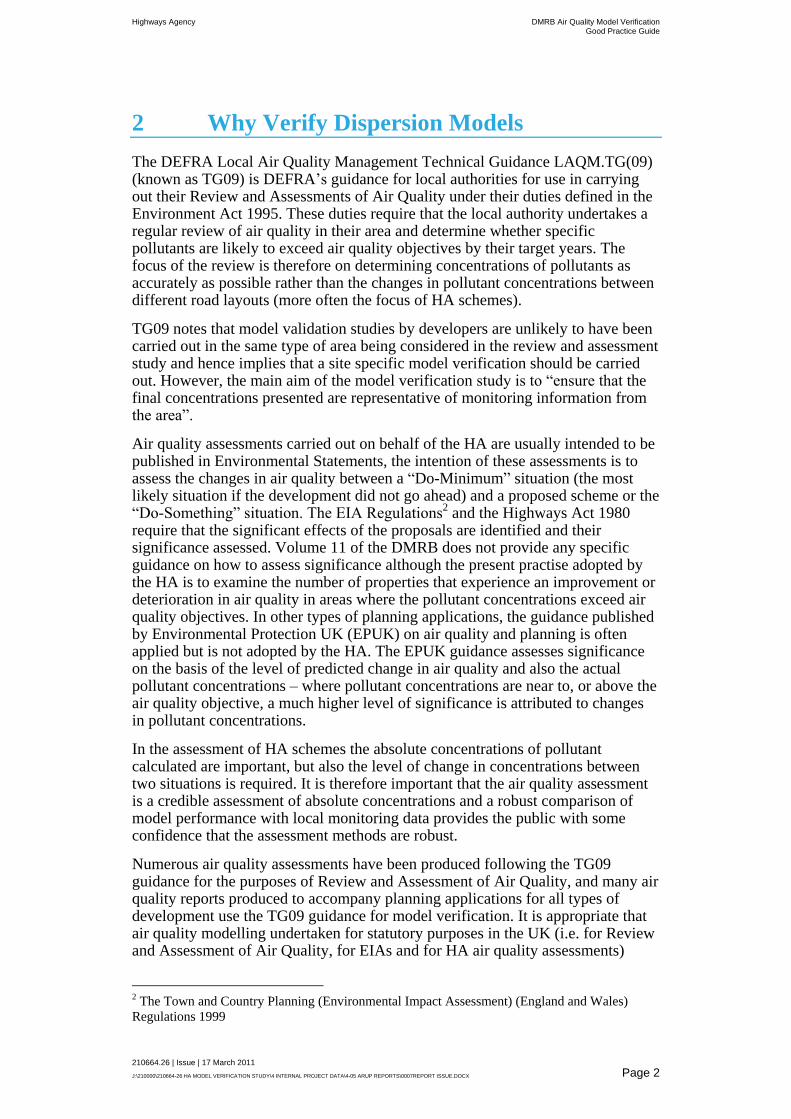
2 Why Verify Dispersion Models
The DEFRA Local Air Quality Management Technical Guidance LAQM.TG(09) (known as TG09) is DEFRA’s guidance for local authorities for use in carrying out their Review and Assessments of Air Quality under their duties defined in the Environment Act 1995. These duties require that the local authority undertakes a regular review of air quality in their area and determine whether specific pollutants are likely to exceed air quality objectives by their target years. The focus of the review is therefore on determining concentrations of pollutants as accurately as possible rather than the changes in pollutant concentrations between different road layouts (more often the focus of HA schemes).
TG09 notes that model validation studies by developers are unlikely to have been carried out in the same type of area being considered in the review and assessment study and hence implies that a site specific model verification should be carried out. However, the main aim of the model verification study is to “ensure that the final concentrations presented are representative of monitoring information from the area”.
Air quality assessments carried out on behalf of the HA are usually intended to be published in Environmental Statements, the intention of these assessments is to assess the changes in air quality between a “Do-Minimum” situation (the most likely situation if the development did not go ahead) and a proposed scheme or the “Do-Something” situation. The EIA Regulations
2 and the Highways Act 1980
require that the significant effects of the proposals are identified and their significance assessed. Volume 11 of the DMRB does not provide any specific guidance on how to assess significance although the present practise adopted by the HA is to examine the number of properties that experience an improvement or deterioration in air quality in areas where the pollutant concentrations exceed air quality objectives. In other types of planning applications, the guidance published by Environmental Protection UK (EPUK) on air quality and planning is often applied but is not adopted by the HA. The EPUK guidance assesses significance on the basis of the level of predicted change in air quality and also the actual pollutant concentrations – where pollutant concentrations are near to, or above the air quality objective, a much higher level of significance is attributed to changes in pollutant concentrations.
In the assessment of HA schemes the absolute concentrations of pollutant calculated are important, but also the level of change in concentrations between two situations is required. It is therefore important that the air quality assessment is a credible assessment of absolute concentrations and a robust comparison of model performance with local monitoring data provides the public with some confidence that the assessment methods are robust.
Numerous air quality assessments have been produced following the TG09 guidance for the purposes of Review and Assessment of Air Quality, and many air quality reports produced to accompany planning applications for all types of development use the TG09 guidance for model verification. It is appropriate that air quality modelling undertaken for statutory purposes in the UK (i.e. for Review and Assessment of Air Quality, for EIAs and for HA air quality assessments)
2 The Town and Country Planning (Environmental Impact Assessment) (England and Wales)
Regulations 1999

Highways Agency DMRB Air Quality Model Verification Good Practice Guide
210664.26 | Issue | 17 March 2011
J:\210000\210664-26 HA MODEL VERIFICATION STUDY\4 INTERNAL PROJECT DATA\4-05 ARUP REPORTS\0007REPORT ISSUE.DOCX Page 3
follow similar procedures to avoid large discrepancies between assessments produced for different purposes.
However, whilst TG09 does provide an approach for model verification, in HA schemes there are often differences in information availability; in particular a much greater level of detail regarding traffic data is available compared with local authority review and assessment studies. HA assessments are also frequently supported with specific local air quality monitoring studies designed to obtain further information regarding the existing background concentrations or specifically installed to be used for model verification purposes. Finally the overall assessment is usually much more detailed than a local authority review and assessment as it has to follow the minimum requirements within the DMRB. The existence of the additional data and the requirement to assess the changes in air quality robustly therefore lead to a need to consider whether additional or adapted model verification procedures would be appropriate for HA air quality studies to build on those detailed in TG09.
Finally, by the use of appropriate model verification procedures, those undertaking air quality modelling studies (including the DMRB air quality spreadsheet and detailed dispersion models) will be able to have much greater confidence in their results and the ability of their models to give a reasonable representation of the air quality conditions in an area.
Highways Agency DMRB Air Quality Model Verification Good Practice Guide
210664.26 | Issue | 17 March 2011
J:\210000\210664-26 HA MODEL VERIFICATION STUDY\4 INTERNAL PROJECT DATA\4-05 ARUP REPORTS\0007REPORT ISSUE.DOCX Page 4
3 Factors Affecting Air Quality Assessments
This section briefly reviews the various inputs into dispersion models and considers their influence on the final modelled result, the uncertainty in the actual input data and how these uncertainties could be reduced.
The final resulting pollutant concentration is made up of a contribution from background sources and from the local road network. The relative contributions from these sources depend on the nature of the area, the distance of the receptor from the main road network and the volume of traffic on the road. In most cases (except very close to the road) the contribution from the background is the most significant contributor and consequently it is important that this is well defined. It is also important to note that, because of this, the contribution from the road network can be relatively small and hence quite large errors in the input data relating to the local roads can have a relatively small impact. For instance, in some cases (particularly in large urban areas), the contribution from the local road network may represent less than 20% of the total observed NOx concentrations (and a much lower proportion for PM10). If the local road contribution was incorrectly estimated by say 50%, the resulting error in the total calculated concentration would only be 10%.
3.1 Traffic Data and Vehicle Emission Factors
The fundamental data required for assessment of the air quality impacts of a road proposal is traffic information, specifically traffic volumes, composition (typically the number of Light Duty vehicles (LDVs) and Heavy Duty Vehicles (HDVs) and speeds). The traffic composition and speed are the key factors in the calculation of vehicle emission rates.
Traffic data are obtained from two sources, firstly, traffic counts carried by various means (e.g. automatic counts, video counts, and manual counting), and secondly, traffic modelling results. Traffic models are mainly designed to predict traffic flows, whilst some information regarding speeds is produced by some models this is considered to be relatively inaccurate by traffic modellers except where newer simulation models are used.
Traffic modelling for HA schemes is always based around a model for peak hours, and while the inter-peak model can be produced, the off peak period is rarely modelled. Air quality assessments are, however, based around the use of Annual Average Daily Traffic (AADT) traffic figures, with the current version of the DMRB Screening Spreadsheet using AADT traffic flows. As the AADT figures are then often scaled for each hour of the day for use in the air quality model, this leads to the situation where traffic data is produced for a specific time period, but then processed to produce an average, but then converted back to a specific time period by the air quality modeller with a subsequent loss of accuracy.
Traffic models are verified by assessing their performance through specific points on the traffic network rather than detailed assessment on a link by link basis. The intention of the modelling process is to be able to predict the overall flows through the network rather than necessarily have an accurate view of flows on a link by link basis. Errors in the assessment of traffic volumes will result in a directly proportional error in the calculation of emissions from the network, i.e. if the flows are underestimated by 10%, so will the emissions.
Highways Agency DMRB Air Quality Model Verification Good Practice Guide
210664.26 | Issue | 17 March 2011
J:\210000\210664-26 HA MODEL VERIFICATION STUDY\4 INTERNAL PROJECT DATA\4-05 ARUP REPORTS\0007REPORT ISSUE.DOCX Page 5
There are significant uncertainties in the assessment of traffic volumes, even where traffic data are obtained from counts where the expectation is of a 20% accuracy, automated methods are less accurate and these also are less able to assess the composition of the traffic.
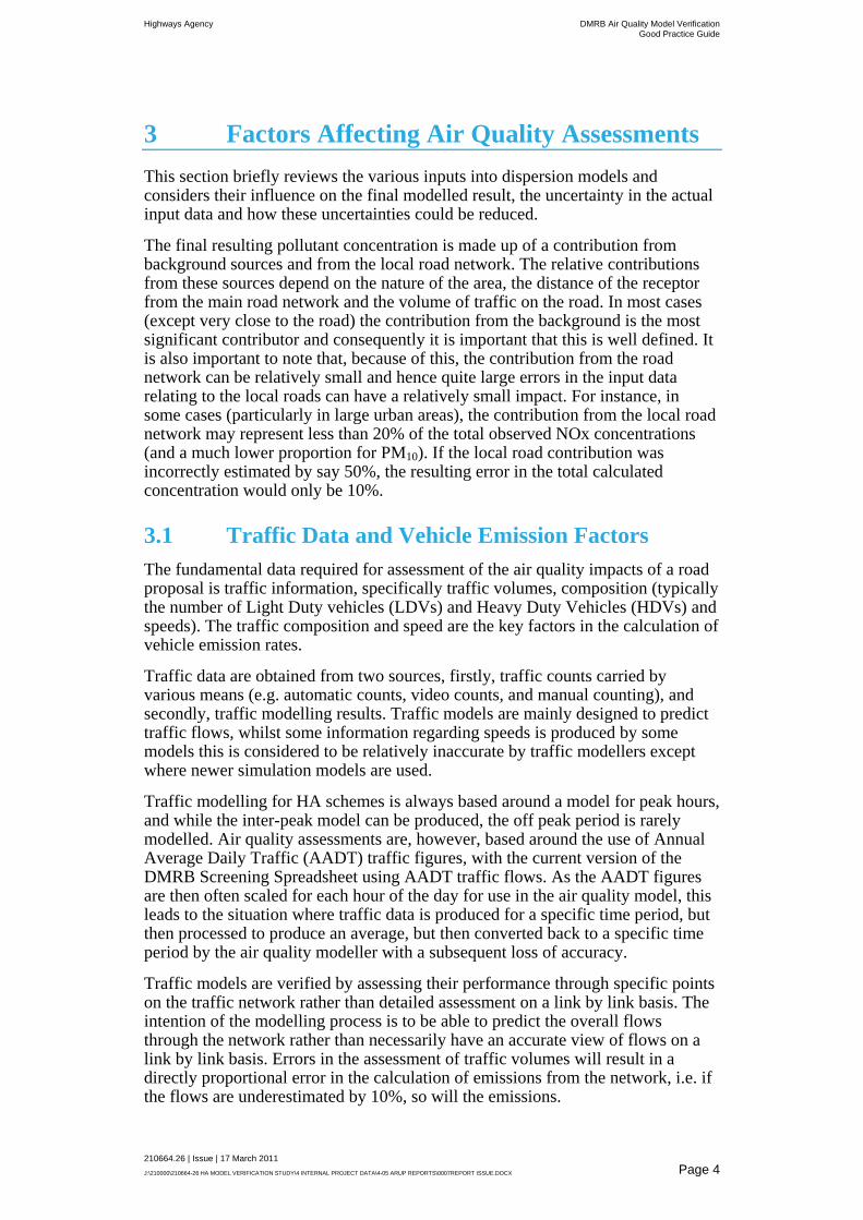
Despite the uncertainties in the assessment of traffic volume, these are much smaller than those that can arise from the combined errors in speed and composition data. Typically HGVs emit around 15 times the pollutant emissions compared with a car. Thus relatively small uncertainties in the composition of the traffic can lead to substantial errors in the emission factors. This can be illustrated using the current Department for Transport (DfT) and Defra Emission Factor Toolkit and examining the changes in the emission rate for nitrogen oxides (NOx) by speed and %HDV.
Figure 1 Change in NOx emission rate as a function of %HDV and speed
0
0.05
0.1
0.15
0.2
0.25
0.3
0.35
0.4
0 5 10 15 20
NO
x Em
issi
on
Rat
e g
/km
/ve
h
%HDV
80 kph
110 kph
140 kph
Highways Agency DMRB Air Quality Model Verification Good Practice Guide
210664.26 | Issue | 17 March 2011
J:\210000\210664-26 HA MODEL VERIFICATION STUDY\4 INTERNAL PROJECT DATA\4-05 ARUP REPORTS\0007REPORT ISSUE.DOCX Page 6
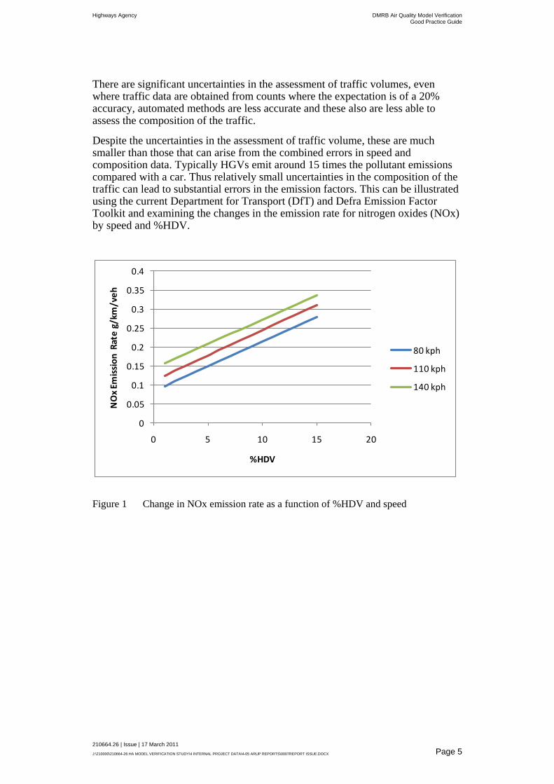
Figure 2 Changes in NOx emission rate as a function of speed and %HDV
Figure 1 and Figure 2 indicate that the %HDV is highly significant in determining the emission rates and is considerably more important than the vehicle speed in terms of the possible errors in estimation of emission rates. Examination of
Figure 2 shows that errors of some 30-60% in NOx emissions are quite conceivable should the estimates of %HGV be estimated incorrectly – for instance, the difference in emission rate at 80kph for an HDV content of 10% and 15% is over 30%.
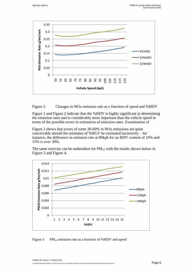
The same exercise can be undertaken for PM10 with the results shown below in Figure 3 and Figure 4.
Figure 3 PM10 emission rate as a function of %HDV and speed
0
0.002
0.004
0.006
0.008
0.01
0.012
0.014
1 2 3 4 5 6 7 8 9 10 11 12 13 14 15
PM
10
Em
issi
on
Rat
e g
/km
/ve
h
%HDV
80kph
110kph
140kph
0
0.05
0.1
0.15
0.2
0.25
0.3
0.35
50
55
60
65
70
75
80
85
90
95
10
0
10
5
11
0
11
5
12
0
NO
x Em
issi
on
Rat
e g
/km
/ve
h
Vehicle Speed (kph)
5% HDV
10%HDV
15%HDV

Highways Agency DMRB Air Quality Model Verification Good Practice Guide
210664.26 | Issue | 17 March 2011
J:\210000\210664-26 HA MODEL VERIFICATION STUDY\4 INTERNAL PROJECT DATA\4-05 ARUP REPORTS\0007REPORT ISSUE.DOCX Page 7
Figure 4 PM10 emission rate as a function of speed and %HDV
The variation in emission rate for PM10 as a function of speed and distance is slightly lower than for NOx but there remains significant potential for errors to be introduced.
It is not likely that the uncertainties in traffic composition and vehicle speed would be consistent across the modelling domain. As noted earlier, there are significant uncertainties in the prediction of vehicle speeds and fleet composition with traffic models. These uncertainties would vary throughout the model,, e.g. speeds may be under or estimated on different links, therefore, a single correction factor applied to the entire model domain is unlikely to be applicable.
3.2 NOx:NO2 Conversion
The final concentration of nitrogen dioxide in the atmosphere depends largely on the conversion of NOx to NO2 in the atmosphere but also on the primary NO2 emissions from the vehicles on the local road network. The reactions involved in the production of NO2 are well documented and although complex, are largely dominated by the oxidation of nitric oxide by ozone. As nitric oxide concentrations near to busy roads are almost always in excess (i.e. there is more nitric oxide (NO) than can be oxidised by the available ozone) the conversion to nitrogen dioxide is highly dependent on local ozone concentrations.
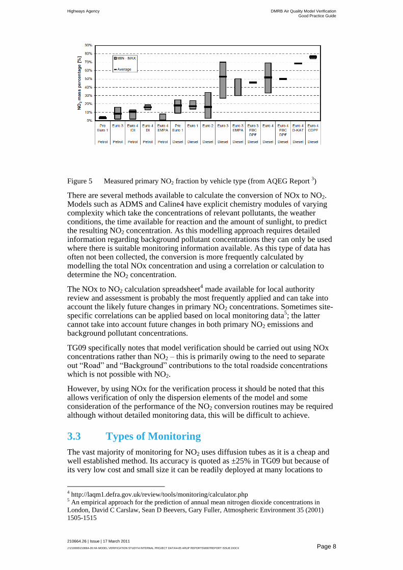
The AQEG3 report on primary NO2 concluded that information was “limited and
uncertain”. However, they also concluded that previous estimates of the primary NO2 fraction of 5% were likely to be underestimates and that some vehicle types had much greater emissions. Figure 5 below shows the measured primary NO2 fraction for various vehicle types.
3 AQEG Report on Primary NO2, 2007
0
0.002
0.004
0.006
0.008
0.01
0.012
0.014
50
55
60
65
70
75
80
85
90
95
10
0
10
5
11
0
11
5
12
0
PM
10
Em
issi
on
rat
e g
/km
/ve
h
Vehicle Speed (kph)
5% HDV
10% HDV
15% HDV
Highways Agency DMRB Air Quality Model Verification Good Practice Guide
210664.26 | Issue | 17 March 2011
J:\210000\210664-26 HA MODEL VERIFICATION STUDY\4 INTERNAL PROJECT DATA\4-05 ARUP REPORTS\0007REPORT ISSUE.DOCX Page 8
Figure 5 Measured primary NO2 fraction by vehicle type (from AQEG Report 3)
There are several methods available to calculate the conversion of NOx to NO2. Models such as ADMS and Caline4 have explicit chemistry modules of varying complexity which take the concentrations of relevant pollutants, the weather conditions, the time available for reaction and the amount of sunlight, to predict the resulting NO2 concentration. As this modelling approach requires detailed information regarding background pollutant concentrations they can only be used where there is suitable monitoring information available. As this type of data has often not been collected, the conversion is more frequently calculated by modelling the total NOx concentration and using a correlation or calculation to determine the NO2 concentration.
The NOx to NO2 calculation spreadsheet4 made available for local authority
review and assessment is probably the most frequently applied and can take into account the likely future changes in primary NO2 concentrations. Sometimes site-specific correlations can be applied based on local monitoring data
5; the latter
cannot take into account future changes in both primary NO2 emissions and background pollutant concentrations.
TG09 specifically notes that model verification should be carried out using NOx concentrations rather than NO2 – this is primarily owing to the need to separate out “Road” and “Background” contributions to the total roadside concentrations which is not possible with NO2.
However, by using NOx for the verification process it should be noted that this allows verification of only the dispersion elements of the model and some consideration of the performance of the NO2 conversion routines may be required although without detailed monitoring data, this will be difficult to achieve.
3.3 Types of Monitoring
The vast majority of monitoring for NO2 uses diffusion tubes as it is a cheap and well established method. Its accuracy is quoted as ±25% in TG09 but because of its very low cost and small size it can be readily deployed at many locations to
4 http://laqm1.defra.gov.uk/review/tools/monitoring/calculator.php 5 An empirical approach for the prediction of annual mean nitrogen dioxide concentrations in
London, David C Carslaw, Sean D Beevers, Gary Fuller, Atmospheric Environment 35 (2001)
1505-1515

Highways Agency DMRB Air Quality Model Verification Good Practice Guide
210664.26 | Issue | 17 March 2011
J:\210000\210664-26 HA MODEL VERIFICATION STUDY\4 INTERNAL PROJECT DATA\4-05 ARUP REPORTS\0007REPORT ISSUE.DOCX Page 9
give good spatial coverage of an area. However, it only measures long term averages (normally monthly) and hence is used in air quality assessment to estimate annual mean concentrations. The results from diffusion tubes need to be corrected to account for laboratory and local bias. The bias adjustment factors can be obtained from national estimates or from local monitoring results. Ideally these devices are used in combination with some continuous monitoring as it allows their performance to be assessed and local bias adjustment factors to be derived.
Continuous monitoring using chemiluminescent devices provides a much more accurate measurement value (±10-15%) and can measure short term hourly average (and less if required). The data obtained are therefore much more extensive and useful for model verification especially in combination with local weather data. In addition, this type of monitor measures both NO and NO2 providing the user with information on total NOx concentrations which are very useful if only the dispersion element of the model requires testing.
The clear disadvantage of diffusion tubes for model verification purposes is that they only measure NO2 and this needs to be converted to NOx using an appropriate method. There are several methods available to this and a calculator is provided as part of the TG09 guidance. Local conversion factors factors can be derived from monitoring data where there are continuous measurements of NOx and nitrogen dioxide, however, there is clearly an additional uncertainty added as part of this process
3.4 Local Site Characteristics
There are clearly some site specific features which affect the final predicted concentration and in some cases will use different modelling procedures. For instance, the presence of road cuttings, street canyons and flyovers can all be accounted for in dispersion models by use of specific model options. However, this will mean that some elements of the model are different and may require different adjustment factors.
Other considerations are where there is complex terrain within the modelling domain which will affect the wind pattern in the area (and consequently dispersion). Some models take account of complex terrain explicitly and models such as ADMS have wind field models that use different modelling approaches. Where there are significant changes in the approach used by the model to account for specific local conditions (e.g. a hill) this can result in differences in model performance that may need to be accounted for separately in the model verification process. This can be achieved by separating the model domain into areas affected significantly by local terrain, and receptors in flatter terrain.
Changes in area type are also important, for example, dispersion is affected by the surface roughness in an area and the models used can take this into account by adjusting how dispersion is calculated (effectively making the atmosphere more turbulent in urban areas). Thus, as the modelling approach is changed, there may be significant differences in model performance between urban and rural areas because the model will address surface turbulence in a different manner.
Highways Agency DMRB Air Quality Model Verification Good Practice Guide
210664.26 | Issue | 17 March 2011
J:\210000\210664-26 HA MODEL VERIFICATION STUDY\4 INTERNAL PROJECT DATA\4-05 ARUP REPORTS\0007REPORT ISSUE.DOCX Page 10
3.5 Projecting Forward
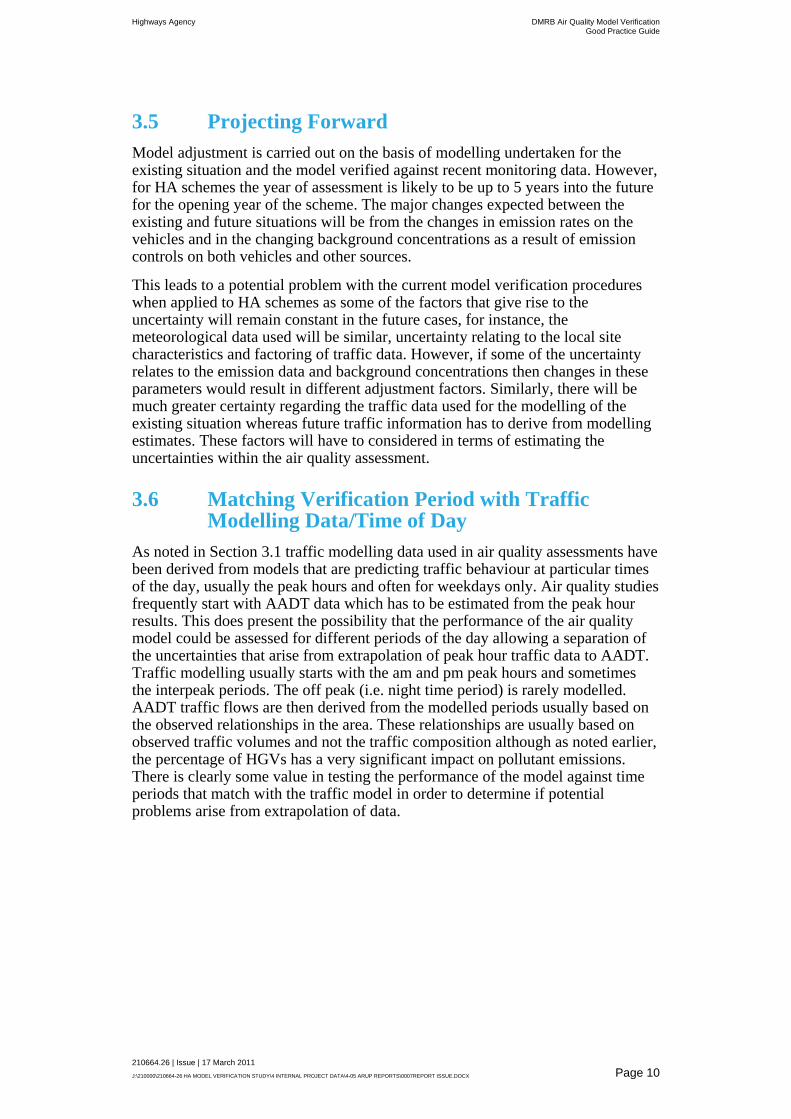
Model adjustment is carried out on the basis of modelling undertaken for the existing situation and the model verified against recent monitoring data. However, for HA schemes the year of assessment is likely to be up to 5 years into the future for the opening year of the scheme. The major changes expected between the existing and future situations will be from the changes in emission rates on the vehicles and in the changing background concentrations as a result of emission controls on both vehicles and other sources.
This leads to a potential problem with the current model verification procedures when applied to HA schemes as some of the factors that give rise to the uncertainty will remain constant in the future cases, for instance, the meteorological data used will be similar, uncertainty relating to the local site characteristics and factoring of traffic data. However, if some of the uncertainty relates to the emission data and background concentrations then changes in these parameters would result in different adjustment factors. Similarly, there will be much greater certainty regarding the traffic data used for the modelling of the existing situation whereas future traffic information has to derive from modelling estimates. These factors will have to considered in terms of estimating the uncertainties within the air quality assessment.
3.6 Matching Verification Period with Traffic Modelling Data/Time of Day
As noted in Section 3.1 traffic modelling data used in air quality assessments have been derived from models that are predicting traffic behaviour at particular times of the day, usually the peak hours and often for weekdays only. Air quality studies frequently start with AADT data which has to be estimated from the peak hour results. This does present the possibility that the performance of the air quality model could be assessed for different periods of the day allowing a separation of the uncertainties that arise from extrapolation of peak hour traffic data to AADT. Traffic modelling usually starts with the am and pm peak hours and sometimes the interpeak periods. The off peak (i.e. night time period) is rarely modelled. AADT traffic flows are then derived from the modelled periods usually based on the observed relationships in the area. These relationships are usually based on observed traffic volumes and not the traffic composition although as noted earlier, the percentage of HGVs has a very significant impact on pollutant emissions. There is clearly some value in testing the performance of the model against time periods that match with the traffic model in order to determine if potential problems arise from extrapolation of data.
Highways Agency DMRB Air Quality Model Verification Good Practice Guide
210664.26 | Issue | 17 March 2011
J:\210000\210664-26 HA MODEL VERIFICATION STUDY\4 INTERNAL PROJECT DATA\4-05 ARUP REPORTS\0007REPORT ISSUE.DOCX Page 11
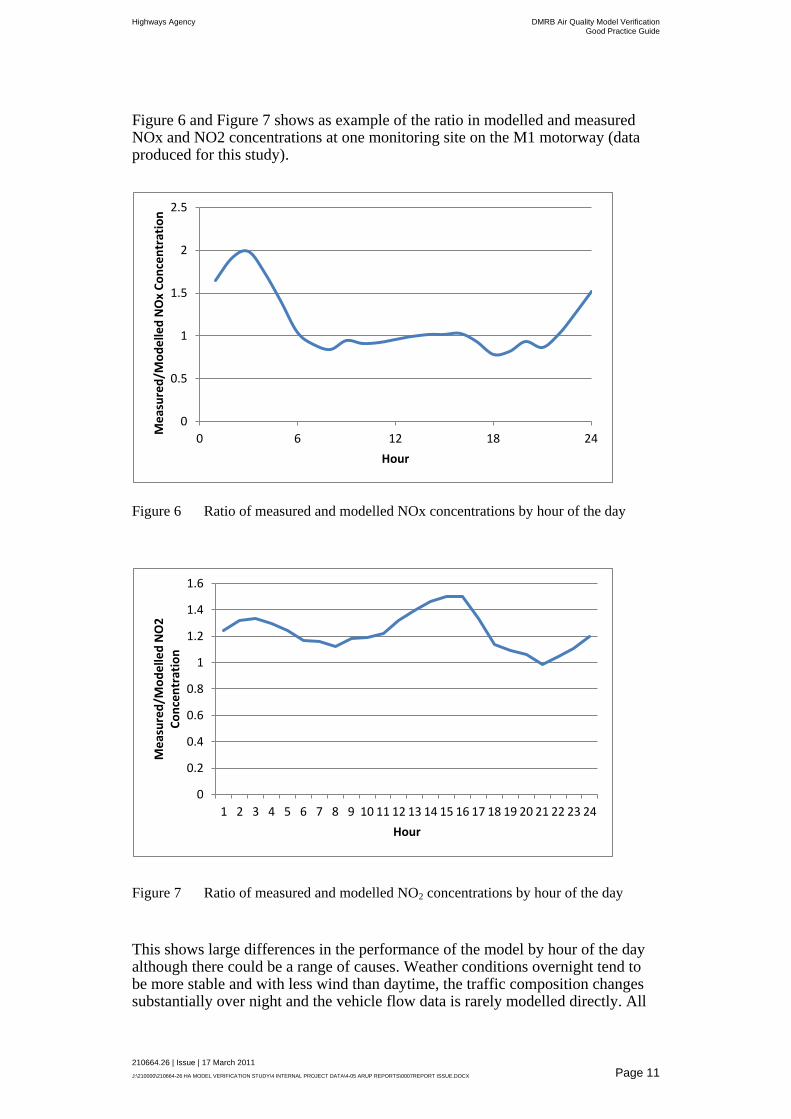
Figure 6 and Figure 7 shows as example of the ratio in modelled and measured NOx and NO2 concentrations at one monitoring site on the M1 motorway (data produced for this study).
Figure 6 Ratio of measured and modelled NOx concentrations by hour of the day
Figure 7 Ratio of measured and modelled NO2 concentrations by hour of the day
This shows large differences in the performance of the model by hour of the day although there could be a range of causes. Weather conditions overnight tend to be more stable and with less wind than daytime, the traffic composition changes substantially over night and the vehicle flow data is rarely modelled directly. All
0
0.5
1
1.5
2
2.5
0 6 12 18 24
Me
asu
red
/Mo
de
lled
NO
x C
on
cen
trat
ion
Hour
0
0.2
0.4
0.6
0.8
1
1.2
1.4
1.6
1 2 3 4 5 6 7 8 9 10 11 12 13 14 15 16 17 18 19 20 21 22 23 24
Me
asu
red
/Mo
de
lled
NO
2
Co
nce
ntr
atio
n
Hour
Highways Agency DMRB Air Quality Model Verification Good Practice Guide
210664.26 | Issue | 17 March 2011
J:\210000\210664-26 HA MODEL VERIFICATION STUDY\4 INTERNAL PROJECT DATA\4-05 ARUP REPORTS\0007REPORT ISSUE.DOCX Page 12
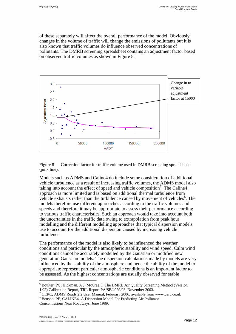
of these separately will affect the overall performance of the model. Obviously changes in the volume of traffic will change the emissions of pollutants but it is also known that traffic volumes do influence observed concentrations of pollutants. The DMRB screening spreadsheet contains an adjustment factor based on observed traffic volumes as shown in Figure 8.
Figure 8 Correction factor for traffic volume used in DMRB screening spreadsheet6 (pink line).
Models such as ADMS and Caline4 do include some consideration of additional vehicle turbulence as a result of increasing traffic volumes, the ADMS model also taking into account the effect of speed and vehicle composition
7. The Caline4
approach is more limited and is based on additional thermal turbulence from vehicle exhausts rather than the turbulence caused by movement of vehicles
8. The
models therefore use different approaches according to the traffic volumes and speeds and therefore it may be appropriate to assess their performance according to various traffic characteristics. Such an approach would take into account both the uncertainties in the traffic data owing to extrapolation from peak hour modelling and the different modelling approaches that typical dispersion models use to account for the additional dispersion caused by increasing vehicle turbulence.
The performance of the model is also likely to be influenced the weather conditions and particular by the atmospheric stability and wind speed. Calm wind conditions cannot be accurately modelled by the Gaussian or modified new generation Gaussian models. The dispersion calculations made by models are very influenced by the stability of the atmosphere and hence the ability of the model to appropriate represent particular atmospheric conditions is an important factor to be assessed. As the highest concentrations are usually observed for stable
6 Boulter, PG, Hickman, A J, McCrae, I. The DMRB Air Quality Screening Method (Version
1.02) Calibration Report, TRL Report PA/SE/4029/03, November 2003. 7 CERC, ADMS Roads 2.2 User Manual, February 2006, available from www.cerc.co.uk 8 Benson, PE, CALINE4- A Dispersion Model For Predicting Air Pollutant
Concentrations Near Roadways, June 1989.
Change in to
variable
adjustment
factor at 15000
AADT
Highways Agency DMRB Air Quality Model Verification Good Practice Guide
210664.26 | Issue | 17 March 2011
J:\210000\210664-26 HA MODEL VERIFICATION STUDY\4 INTERNAL PROJECT DATA\4-05 ARUP REPORTS\0007REPORT ISSUE.DOCX Page 13
atmospheric conditions in combination with higher traffic flows in morning and evening peak hour, this is a particularly important aspect of model performance to investigate particularly as the highest 20% of the hourly NOx contributions often contribute more than 50% of the total annual average (based on observed data next to the M1). Therefore, examination of the model performance for the conditions that give rise to the highest concentrations is particularly important to improve model performance.
3.7 Background Concentrations
As noted earlier, estimates of background concentrations for use in modelling are taken either from a suitable background monitoring site, or more frequently, from the background maps published by DEFRA. Unless installed especially for the project it is rare that a suitable background site will be located in the study area. The background maps are prepared as national estimates based on the National Atmospheric Emissions Inventory and calibrated against observed values. As a national model it clearly cannot be expected that the maps represent an accurate assessment of local conditions, nor can local emission sources necessarily be well represented in a national scale model. This is because the resolution of the sources in a national scale is unlikely to be sufficiently detailed at the local level.
Some estimates of the scale of potential uncertainty in the maps can be found in the AEA report describing the preparation of the maps and the modelling techniques
9. In this report the predictions of background concentrations by the
model is compared with measured values as part of the model calibration exercise, the results are reproduced in Figure 9 .
9 AEA Technology, UK air quality modelling for annual reporting 2007 on ambient air quality
assessment under Council Directives 96/62/EC, 1999/30/EC and 2000/69/EC, January 2009.
Highways Agency DMRB Air Quality Model Verification Good Practice Guide
210664.26 | Issue | 17 March 2011
J:\210000\210664-26 HA MODEL VERIFICATION STUDY\4 INTERNAL PROJECT DATA\4-05 ARUP REPORTS\0007REPORT ISSUE.DOCX Page 14
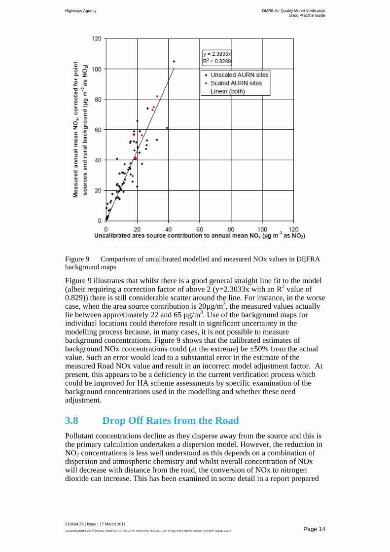
Figure 9 Comparison of uncalibrated modelled and measured NOx values in DEFRA background maps
Figure 9 illustrates that whilst there is a good general straight line fit to the model (albeit requiring a correction factor of above 2 (y=2.3033x with an R
2 value of
0.829)) there is still considerable scatter around the line. For instance, in the worse case, when the area source contribution is 20µg/m
3, the measured values actually
lie between approximately 22 and 65 µg/m3. Use of the background maps for
individual locations could therefore result in significant uncertainty in the modelling process because, in many cases, it is not possible to measure background concentrations. Figure 9 shows that the calibrated estimates of background NOx concentrations could (at the extreme) be ±50% from the actual value. Such an error would lead to a substantial error in the estimate of the measured Road NOx value and result in an incorrect model adjustment factor. At present, this appears to be a deficiency in the current verification process which could be improved for HA scheme assessments by specific examination of the background concentrations used in the modelling and whether these need adjustment.
3.8 Drop Off Rates from the Road
Pollutant concentrations decline as they disperse away from the source and this is the primary calculation undertaken a dispersion model. However, the reduction in NO2 concentrations is less well understood as this depends on a combination of dispersion and atmospheric chemistry and whilst overall concentration of NOx will decrease with distance from the road, the conversion of NOx to nitrogen dioxide can increase. This has been examined in some detail in a report prepared
Highways Agency DMRB Air Quality Model Verification Good Practice Guide
210664.26 | Issue | 17 March 2011
J:\210000\210664-26 HA MODEL VERIFICATION STUDY\4 INTERNAL PROJECT DATA\4-05 ARUP REPORTS\0007REPORT ISSUE.DOCX Page 15
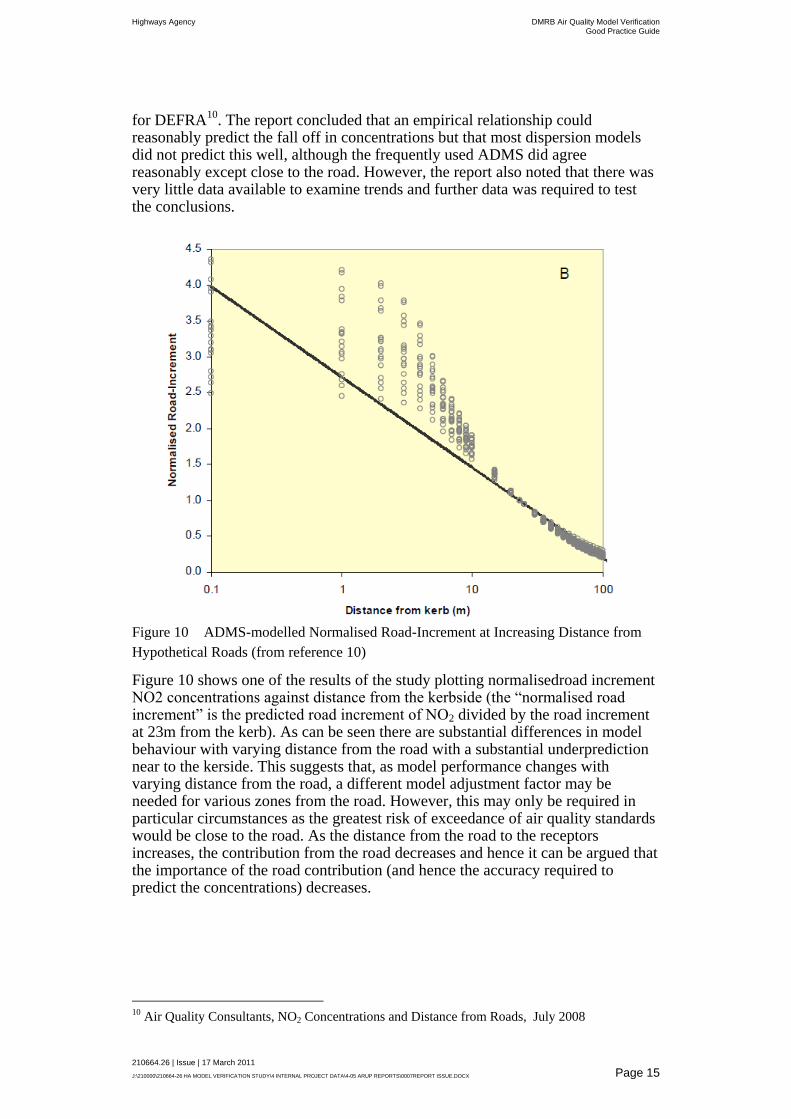
for DEFRA10
. The report concluded that an empirical relationship could reasonably predict the fall off in concentrations but that most dispersion models did not predict this well, although the frequently used ADMS did agree reasonably except close to the road. However, the report also noted that there was very little data available to examine trends and further data was required to test the conclusions.
Figure 10 ADMS-modelled Normalised Road-Increment at Increasing Distance from
Hypothetical Roads (from reference 10)
Figure 10 shows one of the results of the study plotting normalisedroad increment NO2 concentrations against distance from the kerbside (the “normalised road increment” is the predicted road increment of NO2 divided by the road increment at 23m from the kerb). As can be seen there are substantial differences in model behaviour with varying distance from the road with a substantial underprediction near to the kerside. This suggests that, as model performance changes with varying distance from the road, a different model adjustment factor may be needed for various zones from the road. However, this may only be required in particular circumstances as the greatest risk of exceedance of air quality standards would be close to the road. As the distance from the road to the receptors increases, the contribution from the road decreases and hence it can be argued that the importance of the road contribution (and hence the accuracy required to predict the concentrations) decreases.
10 Air Quality Consultants, NO2 Concentrations and Distance from Roads, July 2008
Highways Agency DMRB Air Quality Model Verification Good Practice Guide
210664.26 | Issue | 17 March 2011
J:\210000\210664-26 HA MODEL VERIFICATION STUDY\4 INTERNAL PROJECT DATA\4-05 ARUP REPORTS\0007REPORT ISSUE.DOCX Page 16
3.9 Identifying Verification Zones
Several air quality studies have broken the study area down into different zones and indeed the TG09 approach suggest that different verification areas can be appropriate. Some studies have used GIS to plot out verification patterns and identify trends. Care must be taken with such an approach to account for changes that would be better accounted for in the input data used for the assessment (e.g. meteorological or background data). The rationale for different verification zones can be justified where the dispersion model would use different options for calculations, for instance, street canyons, cuttings, noise barriers and elevated sections of road. In addition, as noted in Section 3.8 there is some evidence that model performance for prediction of drop off rates from the road may depend on distance suggesting that different verification zones may be appropriate.
However, this approach must be used with care to ensure that the changes in adjustment factors are taken into account appropriately. This would seem to be most appropriately applied where the modelling domain can be logically broken down into areas where input data would be different between areas and consequently the uncertainties different. Such a division of the modelling domain should be supported by a statement explaining and justifying the selection of each different area for verification.

Highways Agency DMRB Air Quality Model Verification Good Practice Guide
210664.26 | Issue | 17 March 2011
J:\210000\210664-26 HA MODEL VERIFICATION STUDY\4 INTERNAL PROJECT DATA\4-05 ARUP REPORTS\0007REPORT ISSUE.DOCX Page 17
4 Identifying Approaches to Model Verification
4.1 Review of Current Approaches
There is only one main method used for verification of dispersion models in the UK although there have been some minor variations of the methodology, the method is described in the DEFRA Technical Guidance LAQM.TG(09). Before any model adjustment is considered, the guidance notes that the model set-up and input data should be reviewed carefully to reduce the uncertainties. It notes that common improvements that can be made to a model are:
Checks on traffic data;
Checks on road widths;
Check of distance between sources and monitoring as represented in the model;
Consideration of speed estimates on roads, in particular at junctions where speed limits are unlikely to be appropriate;
Consideration of source type, such as roads and street canyons;
Checks on estimates of background concentrations; and
Checks on the monitoring data.
Only once reasonable efforts have been made to reduce the uncertainties in the modelling process should model adjustment be carried out. Most of these checks are readily achievable, some require checking of the basic geometry in the model, but others, such as the examination of speeds and elements of the traffic data may not be straightforward and will require detailed discussions with the transport assessment team.
Although the method described can be applied using PM10 concentrations, this is rarely undertaken, indeed, in our reviews of Local Authority Review and Assessment reports, this has not been seen described in any report. All model adjustment reported has been for NOx, the Technical Guidance specifically notes not to use NO2 for model adjustment.
For model adjustment, the method is based around the concept of comparing measured and modelled “Road NOx” – i.e. the contribution to the total NOx concentration from the local road network. Modelled Road NOx is readily calculated from a dispersion model by only using the emissions from the road network into the model and ignoring other sources and background concentrations. Measured Road NOx is calculated by subtracting the measured or estimated background concentration from the total measured roadside NOx concentration.
The rationale for using Road NOx rather than the total NOx concentrations is that any model adjustment is only applied to modelled element and not the background concentration. TG09 notes that any adjustment of the background concentration could result in unrealistic estimates of various source contributions. In addition, by taking the road and background contributions separately, projections of
Highways Agency DMRB Air Quality Model Verification Good Practice Guide
210664.26 | Issue | 17 March 2011
J:\210000\210664-26 HA MODEL VERIFICATION STUDY\4 INTERNAL PROJECT DATA\4-05 ARUP REPORTS\0007REPORT ISSUE.DOCX Page 18
concentrations in future years can be more appropriate represented by specifically address the change in emissions from vehicles and in the background concentrations.
A graph of modelled versus measured Road NOx is then prepared and the linear regression trend line determined with the intercept set to 0.The slope of the line is then used as the factor to adjust the modelled road NOx values before adding the background NOx and converting the resulting total NOx concentrations to NO2.
As part of the procedure, the results of the modelling before adjustment should be reviewed to identify whether any consistent trends can be found, in particular, whether different types of areas result in distinctly different adjustment factors. If this is the case, then the guidance suggests calculating a specific adjustment factor for each different type of area.
Adjustment of the background concentration can be undertaken separately when the dispersion model is set up with an emissions inventory and sources to specifically represent the background values.
This method is widely applied in UK air quality studies and has been used on some HA schemes. Given HA schemes can extend over a wider geographic area, the use of different adjustment factors for different geographic areas of the scheme can be applied.
4.2 Potential Issues with TG09 Approach of HA Studies
4.2.1 Use of a single parameter for assessment of model
performance
The TG09 approach is based around the use of a single parameter to assess model performance, i.e. the annual average concentrations. Whilst this is an important outcome of the model it does not examine the actual model performance and it is possible that apparently good model performance (in terms of its apparent ability to model annual average concentrations) has resulted by chance. What this approach does not test is whether the dispersion model is predicting the correct concentrations for the right reasons. This is an issue that has been acknowledged elsewhere
11 and where suitable data exist (essentially data from continuous
monitoring sites) then there is a further opportunity to assess model performance.
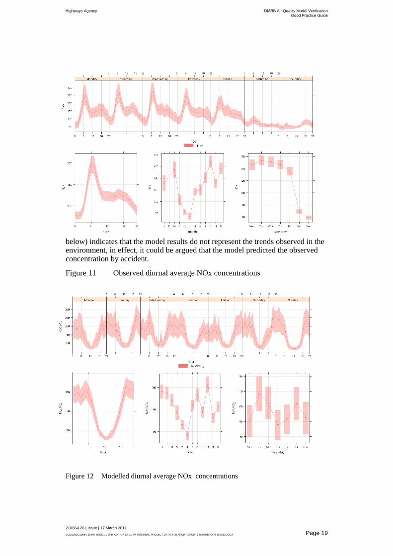
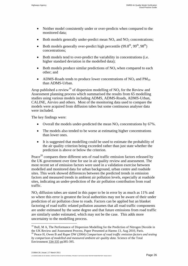
As an example, during recent work undertaken for the HA on the M1 project some initial modelling work was carried out and compared with the results from a roadside monitoring site. AADT traffic flows were entered into the model and the annual mean NO2 concentration calculated. The modelled result was within 2% of the observed annual mean concentration and following the TG09 procedures, no further analysis would be required and no model adjustment would be needed as this passes the initial TG09 test that modelled concentrations of NO2 should be within 25% of monitored values. However, examining the NOx concentrations predicted shows that the model actually over-predicted by 30% and examining the model’s ability to predict the basic temporal trends (see Figure 11 and Figure 12
11 Roger Timmis, Drivers users & approaches for Smarter Air-Quality analysis, Conference
Towards Smarter Air Quality Analysis, Institute of Physics, 1st October 2009
Highways Agency DMRB Air Quality Model Verification Good Practice Guide
210664.26 | Issue | 17 March 2011
J:\210000\210664-26 HA MODEL VERIFICATION STUDY\4 INTERNAL PROJECT DATA\4-05 ARUP REPORTS\0007REPORT ISSUE.DOCX Page 19
below) indicates that the model results do not represent the trends observed in the environment, in effect, it could be argued that the model predicted the observed concentration by accident.
Figure 11 Observed diurnal average NOx concentrations
Figure 12 Modelled diurnal average NOx concentrations

Highways Agency DMRB Air Quality Model Verification Good Practice Guide
210664.26 | Issue | 17 March 2011
J:\210000\210664-26 HA MODEL VERIFICATION STUDY\4 INTERNAL PROJECT DATA\4-05 ARUP REPORTS\0007REPORT ISSUE.DOCX Page 20
This example does illustrate the potential weakness in the examination of one single factor and there are clear advantages in being able to examine further aspects of the model performance. In the example illustrated in Figure 11 and Figure 12 it can be seen that the modelled values:
Do not show the same basic trends in diurnal averages – in the modelled results average concentrations reduce during the daytime and increase at night, reflecting the increase in wind speed and less stable atmosphere during the day;
The peak in concentrations in the morning peak hours (and to a lesser extent the evening peak) are not represented;
The observed trend in average concentrations by day of the week are not represented by the model, the lower concentrations observed at the weekend are not seen in the modelled results;
The changes in diurnal concentration profiles at the weekend are not seen in the modelled results.
This example simply examines model performance in terms of its ability to represent temporal trends, other analyses would also be relevant, particularly the model’s ability to represent the observed trends in relation to meteorological factors such as wind speed, direction and atmospheric stability. This is further discussed in Section 5.3.3.
4.2.2 Assessment of Road NOx
The direct measurement of Road NOx is not usually possible and relies on the existence of suitable monitoring stations or appropriate estimates. In practise it is rare that suitable stations exist and there is a reliance on the use of the background pollutant mapping available on the DEFRA website. Where a remote site is used, then it would be appropriate to include in the air dispersion model the emission sources between the background site and the modelled receptors. In practise, this is rarely undertaken and consequently an underestimate of the background road NOx component will occur.
Similarly, it is possible for the assessment of modelled Road NOx to be significantly in error because some sources maybe ignored in the modelling. Often the roadside concentrations are modelled by taking a remote measurement or estimate of background pollutant concentrations and then only explicitly modelling the local road contributions. This approach ignores any significant sources between the monitoring location and the roadside and hence may well result in concentrations that are too low because sources have not been placed into the model.
These issues act together to result in an apparent under-prediction by the dispersion model and this is a possible explanation of the consistent reported observation in UK Review and Assessments that factors greater than one for model adjustments are required.

Highways Agency DMRB Air Quality Model Verification Good Practice Guide
210664.26 | Issue | 17 March 2011
J:\210000\210664-26 HA MODEL VERIFICATION STUDY\4 INTERNAL PROJECT DATA\4-05 ARUP REPORTS\0007REPORT ISSUE.DOCX Page 21
4.2.3 Linear relationship on regression line
The TG09 approach assumes that any adjustment required is based on a linear relationship – i.e. that the adjustment required is the same for all concentrations modelled. The TG09 approach also forces the regression line through the origin. Whilst the methodology does provide an approach for assessing how robust the background concentrations have been predicted this is only applied where a wide area emissions inventory is used in the modelling. In practise, it is possible that the background concentrations used may not be appropriate or indeed may only be appropriate over one particular area of the modelling domain. There is the possibility that background concentrations may be underestimated in the approach relatively consistently where modellers are using a background site or background estimates that have discounted some local sources. In practise, there are reported results from using this method where forcing the regression line through the origin is clearly inappropriate. Examination of the factors that could rise to model uncertainty shows that some could rise to consistent errors (e.g. meteorological data) whilst other would result in different correction factors across the model domain (e.g. error in vehicle composition or speed data). Table 1 provides a summary of these factors although it should be noted that some of the factors could equally be placed in either category.
Possible consistent factors Variable across the model domain
Vehicle emission data
Meteorological data
NOx:NO2 conversion
Background concentrations
Conversion factors to obtain traffic data (i.e. conversion from peak to AADT)
Meteorological data (local variations)
Traffic data
Vehicle speed assumptions
Terrain type
Special features (e.g. street canyons)
Some meteorological factors influenced by local conditions, e.g. influence of local tall buildings, varying terrain features
Table 1 Factors influencing modelling uncertainty
However, whilst there is no specific justification for a linear relationship, there is similarly no stronger justification for the use of other types of curve fitting and it can be argued that the use of the linear regression represents a pragmatic response to the issue. However, where a verification exercise is carried out, the available data should be examined to determine whether a straight line relationship is necessarily appropriate. Such an examination could consist of plotting the measured and modelled concentrations and testing various relationships for line/curve fitting available within spreadsheet packages or simply by visual examination.
4.2.4 Treatment of background concentrations
Unless modelled explicitly within the study, the TG09 approach makes the assumption that the background concentration used in the modelling is correct by

Highways Agency DMRB Air Quality Model Verification Good Practice Guide
210664.26 | Issue | 17 March 2011
J:\210000\210664-26 HA MODEL VERIFICATION STUDY\4 INTERNAL PROJECT DATA\4-05 ARUP REPORTS\0007REPORT ISSUE.DOCX Page 22
forcing the regression line through the origin. This assumption is not easy to justify, as noted earlier, the use of background mapped data as associated uncertainties and even the use of locally measured background data does not give a complete assessment of concentrations. In a current monitoring study being carried out on one HA scheme NOx concentrations measured at the roadside site are lower than those at a nearby background site for around 15% of the year, in this case, this can be attributed to the two stations being on the eastern and western sides of the motorway involved and even though the background site is more than 1km from the road, the concentrations recorded at the background site must therefore be affected by other pollutant sources that do not significant impact on concentration near the motorway.
This has certainly resulted in some instances reported in Review and Assessments where the line of best fit would clearly not pass through the origin (see Figure 13 below). It is clearly credible that errors in the overall modelled concentrations could derive from the treatment of background concentrations in the modelling and it is considered that this approach could be reviewed for use in HA studies.
Figure 13 Example model verification regression line for NO2 (with regression lines forced through 0,0, and standard regression)
4.3 Review of Published Model Validation Studies
Models commonly used in the UK for traffic assessments include ADMS-Roads, ADMS-Urban, the DMRB spreadsheet, Caline4 and Breeze-Roads. Each has its merits and complexities and each can be the right choice for a particular modelling study. Where air quality standards are unlikely to be exceeded and the expected changes in the traffic are small, then a screening approach such as the DMRB spreadsheet is appropriate. For more complex situations where specific local features need assessment, then a model that can take these into account
y = 0.8252x
y = 0.25x + 9.08
0
5
10
15
20
25
0 5 10 15 20 25 30
Me
asu
red
NO
2 C
on
cen
trat
ion
s (p
pb
)
Monitored NO2 concentrations ppb

Highways Agency DMRB Air Quality Model Verification Good Practice Guide
210664.26 | Issue | 17 March 2011
J:\210000\210664-26 HA MODEL VERIFICATION STUDY\4 INTERNAL PROJECT DATA\4-05 ARUP REPORTS\0007REPORT ISSUE.DOCX Page 23
should be sued, for examples, where there is a street canyon, a model such as ADMs-Roads can take these into account.
The developers of models (e.g. CERC, USEPA) have published validation and intercomparison studies to demonstrate the accuracy and precision of their models. In addition third party comparisons of modelled and monitored data published in the scientific literature can also be taken as validation studies. It is not surprising that validation studies show models to be performing well or at least not badly; approaches to modelling any one situation can vary and with reasonable assumption models can still produce a wide variety of predictions. Model developers are unlikely to publish studies that show their models are not performing well. Many of the equations used within models are also derived or modified by using datasets against which they are validated
12. Hence, validation
by comparison of the model output with these same datasets is somewhat tautological. Overall, model developers report results that do not suggest any consistent significant under or over prediction with their models. For instance, the Caline4 manual
13 reports the results of their model performance and publishes a
series of model performance assessment graphs, an example is illustrated in Figure 14 which shows that when comparing measured and modelling values, the results are scattered around the 1:1 line.
12
Venkatram A, Karamchandani P, Pai P and Goldstein R (1994) The development and
applications of a simplified ozone modelling system Atmospheric Environment 22, pp3665-3678. 13 Benson, P E, CALINE4- A Dispersion Model For Predicting Air Pollutant
Concentrations Near Roadways, Caltrans, November 1984.

Highways Agency DMRB Air Quality Model Verification Good Practice Guide
210664.26 | Issue | 17 March 2011
J:\210000\210664-26 HA MODEL VERIFICATION STUDY\4 INTERNAL PROJECT DATA\4-05 ARUP REPORTS\0007REPORT ISSUE.DOCX Page 24
Figure 14 Model performance assessment for Caline4

Highways Agency DMRB Air Quality Model Verification Good Practice Guide
210664.26 | Issue | 17 March 2011
J:\210000\210664-26 HA MODEL VERIFICATION STUDY\4 INTERNAL PROJECT DATA\4-05 ARUP REPORTS\0007REPORT ISSUE.DOCX Page 25
Similar studies14
have been carried out for the ADMS-Roads model with results that show a scatter around the 1:1 line when comparing measured and modelled concentrations of a tracer gas, an example is shown in Figure 15.
Figure 15 Model performance evaluation for ADMS-Roads
CERC published a validation study15
of ADMS-Urban and ADMS-Roads using monitoring data from the M4 and M25 motorways. Monitoring of NO2, NOx and PM10 data from 1997 and 1996 were compared to predictions using background data for NOx and O3 from monitoring sites and the NETCEN gridded emissions database. Some manipulation of the background data was done to try and make it more representative of the M4/M25 locations. Comparison statistics including means, correlation, and bias were generated using a software package (BOOT
16)
excluding any hours when all three required datasets17
were available. The paper revealed
18 the following:
Both models show reasonably good agreement with measured data;
14 Validation of ADMS-Roads using the CALTRANS Highway 99 dataset, available on
http://www.cerc.co.uk/environmental-software/model-documentation.html 15 CERC (1991) ADMS-Urban and ADMS-Roads Validation, Validation Against M4 and M25
Motorway Data www.cerc.co.uk/PROMOTE/Urban_M25_Validation.pdf 16 Hanna SR, Strimaitis DG and Chang JC (1991) Hazard Response modelling Uncertainty (A
Quantitative Method) Sigma Research Corporation Report. 17 Background monitoring data, roadside monitoring data and meteorological data. 18 The publication produces tables of comparison data and does not summarise or conclude, hence
the conclusions are those drawn by ARUP from the data tables.
Highways Agency DMRB Air Quality Model Verification Good Practice Guide
210664.26 | Issue | 17 March 2011
J:\210000\210664-26 HA MODEL VERIFICATION STUDY\4 INTERNAL PROJECT DATA\4-05 ARUP REPORTS\0007REPORT ISSUE.DOCX Page 26
Neither model consistently under or over-predicts when compared to the monitored data;
Both models generally under-predict mean NOx and NO2 concentrations;
Both models generally over-predict high percentile (99.8th
, 99th
, 98
th)
concentrations;
Both models tend to over-predict the variability in concentrations (i.e. higher standard deviation in the modelled data);
Both models produce similar predictions of NOx when compared to each other; and
ADMS-Roads tends to produce lower concentrations of NO2 and PM10 than ADMS-Urban.
Arup published a review19
of dispersion modelling of NO2 for the Review and Assessment planning process which summarised the results from 65 modelling studies using various models including ADMS, ADMS-Roads, ADMS-Urban, CALINE, Airviro and others. Most of the monitoring data used to compare the models were acquired from diffusion tubes but some continuous analyser data were included.
The key findings were:
Overall the models under-predicted the mean NO2 concentrations by 67%.
The models also tended to be worse at estimating higher concentrations than lower ones.
It is suggested that modelling could be used to estimate the probability of the air quality criterion being exceeded rather than just state whether the prediction is above or below the criterion.
Peace20
compares three different sets of road traffic emission factors released by the UK government over time for use in air quality review and assessment. The most recent set of emission factors were used in a validation exercise between modelled and monitored data for urban background, urban centre and roadside sites. This work showed differences between the predicted trends in emission factors and measured trends in ambient air pollution levels, especially at roadside sites, indicating an under-prediction of the air pollution contribution from road traffic.
NO2 diffusion tubes are stated in this paper to be in error by as much as 11% and
so where this error is greatest the local authorities may not be aware of their under
prediction of air pollution close to roads. Factors can be applied but an blanket
factoring of road traffic related pollution assumes that all road traffic components
are under estimated by the same degree and that future emissions from road traffic
are similarly under estimated, which may not be the case. This adds more
uncertainty to the modelling process.
19 Bull, M A, The Performance of Dispersion Modelling for the Prediction of Nitrogen Dioxide in
the UK Review and Assessment Process, Paper Presented at Harmo 13, Aug 2010, Paris. 20 Peace H, Owen B and Raper DW (2004) Comparison of road traffic emission factors and testing
by comparison of modelled and measured ambient air quality data. Science of the Total
Environment 334-335 pp385-395.

Highways Agency DMRB Air Quality Model Verification Good Practice Guide
210664.26 | Issue | 17 March 2011
J:\210000\210664-26 HA MODEL VERIFICATION STUDY\4 INTERNAL PROJECT DATA\4-05 ARUP REPORTS\0007REPORT ISSUE.DOCX Page 27
Owen et al21
describes the use of urban emission inventory data and the
ADMS-Urban model to calculate concentrations of NOx and NO2 in London.
Summer and winter predictions were compared to observed data at four locations,
two locations in Central London and two in East London. The performance of the
model in terms of estimating the atmospheric chemistry is evaluated. Comparison
of modelled and monitored data was reasonable but the model tended to
underestimate concentrations of NOx during the winter months. Hour by hour
time series comparisons of NOx showed some agreement but the study concluded
that the model may show a tendency to under-predict concentrations of NOx
during cold, stable atmospheric conditions. The high percentile values (95th
to
100th
of hourly data) of NO2 predicted by the chemistry model did not show such
good agreement.
Righi22
examines how well ADMS-Urban performs in a medium-sized town in
Italy where vehicle traffic accounts for most of the carbon monoxide (CO)
emissions. ADMS-Urban is found to perform satisfactorily, the study shows that
the model tends to underestimate values by 10-25% compared to measured values.
Performance is found to depend on some meteorological parameters with the
model doing significantly worse at higher (>4m/s) wind speeds. The orientation of
the local streets to the monitoring stations also had an effect on model agreement,
especially at low (<4m/s) wind speeds. The best agreement between modelled
and monitored occurred during highly unstable conditions when pollutants
disperse rapidly which is well represented in the model. Some of the differences
were attributed to the model not allowing pollution to build up over several hours
(a fault of all such steady state Gaussian-type models not just ADMS).
Comparison of modelled running means (which will smooth out the peaks)
showed better agreement with the monitored data.
Holmes et al23
reviewed the performance of 29 separate and widely different models to estimate particle dispersion. The models ranged from simple box type models (e.g. AURORA), Gaussian models (including Caline4, Calpuff, AERMOD, UK-ADMS and Screen3), to Lagrangian, Eulerian and complex fluid dynamics (CFD) models. The study did not rank the models as whilst one model might perform better than in another one study the results may be reversed in a different scenario. The study indentified that the complexity of the environment, the dimensions of the model, the nature of the particle source, the computing power and time that is required and the accuracy and time scale of the calculated concentrations desired can all be critical factors in model choice. The study found that gas phase dispersion models seem reasonably accurate with respect to calculating average daily and annual particle mass concentrations in simple and regional domains but less good when atmospheric chemistry was important in
21 Owen B, Edmunds HA, Carruthers DJ, and Singles RJ (2000) Prediction of total oxides of
nitrogen and nitrogen dioxide concentrations in a large urban area using a new generation urban
scale dispersion model with integral chemistry model Atmospheric Environment 34 pp397-406. 22 Righi S, Lucialli P and Pollini E (2009) Statistical and diagnostic evaluation of the ADMS-
Urban model compared with an urban air quality monitoring network Atmospheric Environment
43 pp3850–3857. 23 Holmes NS and Morawska L (2006) A review of dispersion modelling and its application to the
dispersion of particles: An overview of different dispersion models available Atmospheric
Environment 40 pp5902–5928.
Highways Agency DMRB Air Quality Model Verification Good Practice Guide
210664.26 | Issue | 17 March 2011
J:\210000\210664-26 HA MODEL VERIFICATION STUDY\4 INTERNAL PROJECT DATA\4-05 ARUP REPORTS\0007REPORT ISSUE.DOCX Page 28
particle formation or when other statistics were required. Comparisons of two or three models to validation data sets has been done but not for all models reviewed. Many of the models reviewed in the paper are not commercially available and so have restricted applications. The paper did not recommend any specific models but suggested that the user would need to review the type of modelling required and data availability and select an appropriate model from those available.
4.4 Performance of Models in the UK
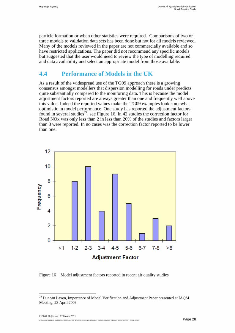
As a result of the widespread use of the TG09 approach there is a growing consensus amongst modellers that dispersion modelling for roads under predicts quite substantially compared to the monitoring data. This is because the model adjustment factors reported are always greater than one and frequently well above this value. Indeed the reported values make the TG09 examples look somewhat optimistic in model performance. One study has reported the adjustment factors found in several studies
24, see Figure 16. In 42 studies the correction factor for
Road NOx was only less than 2 in less than 20% of the studies and factors larger than 8 were reported. In no cases was the correction factor reported to be lower than one.
Figure 16 Model adjustment factors reported in recent air quality studies
24 Duncan Laxen, Importance of Model Verification and Adjustment Paper presented at IAQM
Meeting, 23 April 2009.

Highways Agency DMRB Air Quality Model Verification Good Practice Guide
210664.26 | Issue | 17 March 2011
J:\210000\210664-26 HA MODEL VERIFICATION STUDY\4 INTERNAL PROJECT DATA\4-05 ARUP REPORTS\0007REPORT ISSUE.DOCX Page 29
In other Review and Assessment reports, adjustment factors up to 24 have been reported
25. This level of adjustment suggests a much higher degree of uncertainty
in the modelling that can be explained by the possible errors in the input data and does not compare well with the results reported in model validation studies. These high values may partly be explained by the fact that fairly substantial errors cold be introduced in the calculation of Road-NOx because it is generally a relatively small number calculated by subtracting two larger numbers (i.e. total Road-NOx – Total Background NOx). A smaller correction factor would be required if total NOx concentrations were being examined.
In a study compiling the unadjusted results for NO2 modelling in UK Review and Assessments
19, the same level of under prediction was not found, indeed the
results did appear to be reasonably well scattered around a 1:1 straight line (although this study was carried out comparing NO2 concentrations). A summary of the results is shown in Figure 17 which compares predicted and measured total NO2 concentrations (i.e. not the Road component).
Figure 17 Comparison of predicted and measured NO2 concentrations from UK Reviews and Assessments
The level of adjustment factors found using the TG09 approach is not consistent with either the model developers’ model verification studies, or the overall performance reported elsewhere for dispersion models. This may suggest a problem with the estimation of the Road NOx component and particularly that Background NOx could be underestimated (i.e. leading to an overestimate of the Road NOx). A particular issue with interpreting these results is the very limited information available for NOx concentrations near to roads with the vast majority of information derived from diffusion tube measurements of NO2 only. This leads
25 Preston City Council, Air Quality Detailed Assessment, November 2004.
0
10
20
30
40
50
60
70
80
90
100
0 10 20 30 40 50 60 70 80 90 100
Measure
d N
O2 c
oncentr
atio
ns µ
g/m
3
|Predicted NO2 Concentrations µg/m3

Highways Agency DMRB Air Quality Model Verification Good Practice Guide
210664.26 | Issue | 17 March 2011
J:\210000\210664-26 HA MODEL VERIFICATION STUDY\4 INTERNAL PROJECT DATA\4-05 ARUP REPORTS\0007REPORT ISSUE.DOCX Page 30
to an additional possible error from the conversion of the NO2 diffusion tube results to NOx concentrations.
4.5 Pollutants to be Used in Verification
The vast majority of air quality issues that occur in the UK relate to NO2, PM10 is a lesser problem and there are only a few areas in the country that are now considered to be unlikely to meet the EU limit value for this pollutant. Model verification procedures should therefore concentrate on the requirements for assessing concentrations of nitrogen dioxide. The choices are therefore either the use of nitrogen dioxide or nitrogen oxides. The use of another pollutant as a proxy is not suitable as there is little monitoring information for any other pollutants, indeed, NO2 is the most widely monitored pollutant in the UK owing to the widespread use of diffusion tubes.
In many respects the use of NO2 for verification has many advantages, particularly as most monitoring is for NO2 and not for nitrogen oxides as the latter requires the use of continuous monitors that are expensive and require sites with power and security. NO2 can be measured with diffusion tubes which is a technique widely applied in the UK and where the limitations of the method are well known. Although diffusion tubes exist for nitrogen oxides, they are not widely applied and experience on a recent HA air quality monitoring project on the M1 conducted by Arup suggests the results from this method are very variable and did not compare well with the results from continuous monitoring. The use of NO2 diffusions tube result to calculate NOx concentrations (which is widely applied) clearly can introduce further uncertainty into the verification process.
The advantage of using NO2 for verification is that many models are able to directly calculate this pollutant using internal chemistry modules that calculate the conversion of NOx to NO2. The results can then be compared with monitoring that directly measures the pollutant. Most monitoring is carried out using nitrogen dioxide diffusion tubes and consequently, if NOx is used as the pollutant to verify the modelling process, the results from monitoring need to be converted from NO2 to NOx resulting in the introduction of further uncertainty.
However, it can be argued that the same issue of uncertainty arises with the use of NO2 as the pollutant as modelling of NO2 is essentially a two stage process; firstly a calculation of the dispersion of the exhaust gases and then secondly the assessment of the conversion of NOx to NO2. The latter introducing the same uncertainty as the conversion of a NO2 diffusion tube result to nitrogen oxides. By using NOx as the pollutant for verification purposes, the performance of the dispersion elements of the modelling can be separated from the atmospheric chemistry aspects. This is important as the main functions of the model are to calculate dispersion in the atmosphere whilst the chemistry elements of the model usually take place after the dispersion has been calculated. By separating examining the dispersion and chemistry element the user may be able to specifically identify areas where the model is not performing well.
Furthermore, the emission data used in dispersion modelling is based on NOx emissions and it is important that future changes in these emissions are properly represented in the verification process. By applying a verification factor to the NOx values in the modelling, the future changes in emissions are likely to be better represented.

Highways Agency DMRB Air Quality Model Verification Good Practice Guide
210664.26 | Issue | 17 March 2011
J:\210000\210664-26 HA MODEL VERIFICATION STUDY\4 INTERNAL PROJECT DATA\4-05 ARUP REPORTS\0007REPORT ISSUE.DOCX Page 31
Finally it is very difficult to separate out the NO2 emitted from vehicles on the road and the background sources because of atmospheric chemistry. Although it is straightforward to subtract background from roadside NO2 measurements this process would be very likely to underestimate the contribution from the road as conversion of NOx to NO2 is frequently ozone limited and therefore there will be NOx emitted from the local road network that would be unaccounted for in the verification process.
These difficulties do not necessarily rule out the use of NO2 as the pollutant used for verification but that any approach based around this pollutant would not be able to distinguish between the contribution of the road and background sources. Whilst this would create some difficulties in predicting future concentrations it could be argued that there are already considerable problems in successfully predicting the future levels and this would only add a further small uncertainty.
Highways Agency DMRB Air Quality Model Verification Good Practice Guide
210664.26 | Issue | 17 March 2011
J:\210000\210664-26 HA MODEL VERIFICATION STUDY\4 INTERNAL PROJECT DATA\4-05 ARUP REPORTS\0007REPORT ISSUE.DOCX Page 32
5 Recommendations for Verification Approach
5.1 Overall Approach for Verification
The approach to be used for model verification will depend on the type of monitoring information available. If only diffusion tube measurements are available then the only approach that can be used would be to use the annual average NO2 concentration, possibly converted to NOx. The approach for model verification also depends on the traffic data available, for instance where specific traffic models have been developed for peak (am and pm) and off peak periods this would allow assessment of model performance specifically for these periods.
It is not recommended that a single process be used for model verification in all HA air quality assessments but that a section of the air quality assessment report should be devoted to reporting a Model Performance Evaluation and justifying the approach taken in the assessment. The aim of this Evaluation should be to provide confidence that the modelling study can predict pollutant concentrations with the required accuracy and that the model predicts the correct concentrations for the right reasons – i.e. that the model represents the trends observed in the environment.
The subsequent elements of this section provide suggested approaches that can be used to demonstrate confidence in the modelling results. The actual approach used will depend on the data availability and the significance of the final modelled values. The latter requires some assessment of the risk of exceeding an air quality objective or limit value with the proposed scheme in place. If the risk is considered to be low, then detailed model verification is less likely to be required. Note that the suggested approaches are not specific to a particular pollutant and can be readily applied to any pollutant.
5.2 Model Verification Approach with Annual Mean Data
Many assessments may not have access to monitoring data from a suitable continuous monitoring site for model verification purposes and hence model verification would have to be based on annual mean NO2 concentrations obtained from diffusion tube monitoring. When the data available for assessment of model performance are limited the aim of the verification exercise should still be to demonstrate confidence in the model performance.
TG09 gives an approach that would allow consistency with most air quality studies carried out in the UK. However, if this approach is used, then the Model Performance Evaluation of the air quality assessment should specifically address the uncertainties in input data and model, examining the factors suggested in TG09 explicitly to justify the input into the model and the model options used and discuss the range of options considered within the study. These factors are:
checks on traffic data;
checks on road widths;
Highways Agency DMRB Air Quality Model Verification Good Practice Guide
210664.26 | Issue | 17 March 2011
J:\210000\210664-26 HA MODEL VERIFICATION STUDY\4 INTERNAL PROJECT DATA\4-05 ARUP REPORTS\0007REPORT ISSUE.DOCX Page 33
checks on distance between sources and monitoring as represented in the model;
consideration of speed estimates on roads in particular at junctions where speed limits are unlikely to be appropriate;
consideration of source type, such as roads and street canyons;
checks on estimates of background concentrations; and
checks on the monitoring data.
When moving on to consider comparison of measured and modelled data it is proposed that consideration is given to the identification of specific areas of the modelling domain where the model performance may be substantially different and model performance should be assessed separately. Whilst this is a similar approach to that suggested in TG09, the main difference is a consideration at the start of the Model Performance Evaluation of where these different verification zones should exist and assess these separately. The following are possible factors for examination in the model verification, it is not suggested that all of these necessarily be examined in the model evaluation but only those that are relevant to the particular study and where the results will be significant (i.e. areas where air quality is of particular concern):
distance from road;
volume of traffic;
composition of traffic – particularly where large changes in %HGV are expected;
orientation of monitoring site in relation to the major road and meteorological conditions;
areas where monitored meteorological conditions may not reflect local conditions (e.g. complex terrain, distance from meteorological monitoring station used in the assessment;
where there are significant difference in site characteristics (e.g. urban/ rural areas, areas close to coast or water bodies);
where the scheme features particular features such as cuttings, flyovers, street canyons.
Within the Model Performance Evaluation, the influence of the relevant factors above should be considered and separately assessed if considered to be significant.
One useful analysis within the Model Performance Evaluation would be the plotting and collation of the various adjustment factors that have calculated at each model verification point. Some users have found it a useful exercise to plot these on maps to identify trends in verification factors. In addition, a frequency plot of the various adjustment factors derived would provide a useful a useful indication of the consistency of the model results.
Highways Agency DMRB Air Quality Model Verification Good Practice Guide
210664.26 | Issue | 17 March 2011
J:\210000\210664-26 HA MODEL VERIFICATION STUDY\4 INTERNAL PROJECT DATA\4-05 ARUP REPORTS\0007REPORT ISSUE.DOCX Page 34
It is considered that particular attention should be paid to the calculation of monitored and modelled Road-NOx. As noted in Section 4.2.2, there does appear to be considerable potential for errors to be made with this parameter.
It is also recommended that the performance of the model should include a specific assessment of the background concentrations and when following the TG09 approach plotting measured and modelled Road-NOx the applicability of forcing the regression line through the origin should be considered.
5.3 Model Verification Approach where Continuous Monitoring Data are Available
Where continuous monitoring data are available this allows the Model Performance Evaluation to look beyond comparison with a single monitored value. The model performance can be assessed in terms of its ability to represent the trends in concentrations observed in the environment. It also allows the selection of data to determine model performance at particular periods of the day, for particular meteorological conditions and the rejection of periods when the concentrations are not influenced by emissions from the nearby roads (i.e. when the wind is blowing from the receptor towards the main road). The latter is important as this can be used to select the time periods where the model has some influence on the final result and reject those periods where the modelled concentration has no influence (i.e. when effectively the background concentration input into the model is the final result).
The ability to assess model performance in more detail can be considered to be an extension of the first step suggested in TG09 where it suggests that model set up and the input data be examined in more detail. Following these stage, it is possible that the TG09 approach for final model adjustment could be used.
The following stages in the process are proposed assuming that at least one year of monitored NOx and NO2 data are available and a dispersion model has been run to predict hourly concentrations for the same year using appropriate meteorological data.
It is proposed that the following factors are checked in the model performance evaluation.
5.3.1 Basic Statistical Performance Evaluation
A basic assessment of model performance should be carried out by plotting measured against modelled concentrations on an XY plot, together with comparison of basic statistics (mean, median, standard deviation). Consideration should be given to examining only the relevant data for model performance, in some instances, (for instance where there is a single road being examined), the road emissions will only affect predicted concentrations when the wind direction is blowing from the road to the monitoring point. When the wind is in other directions, then the predicted concentrations will only be the input background concentrations and are not affected by the dispersion model unless receptors are located very close to the road where pollutant concentrations are affected by the model’s treatment of mechanical turbulence caused by vehicle movements.
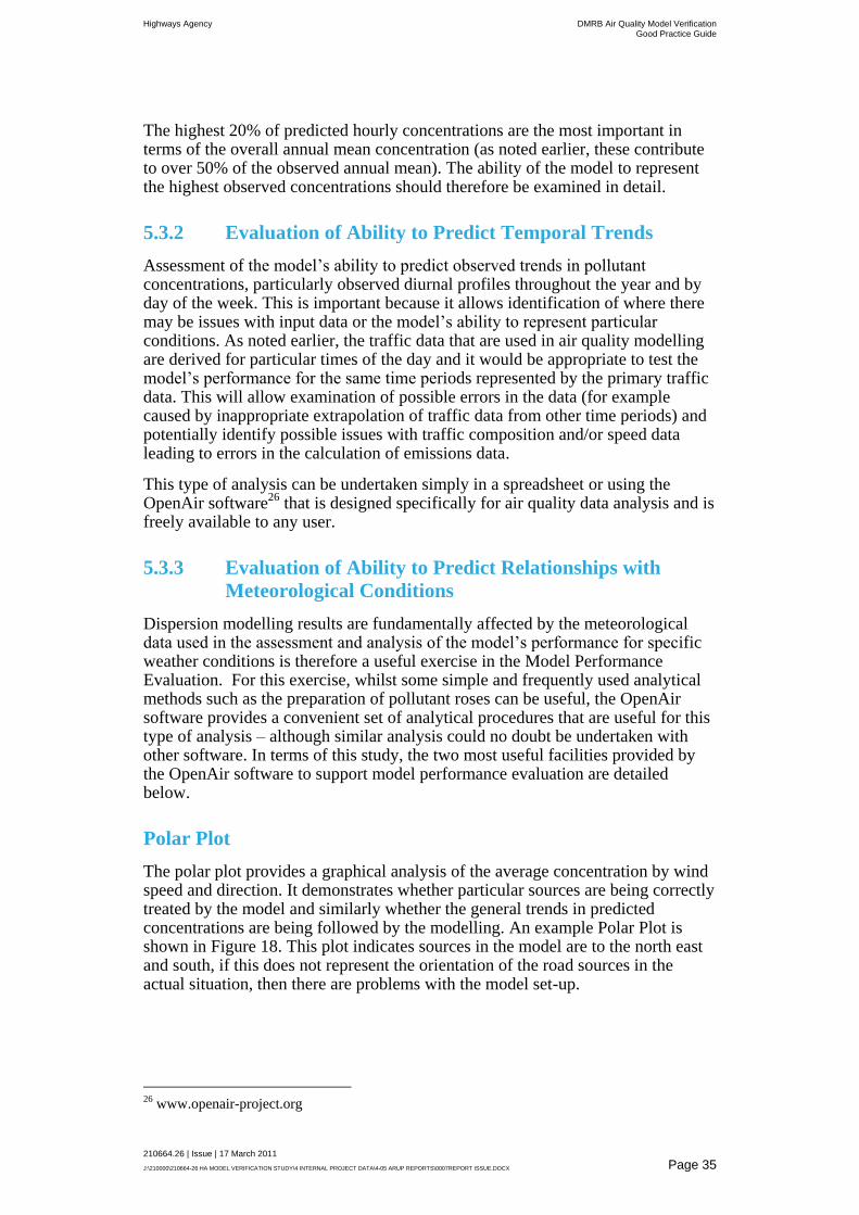
Highways Agency DMRB Air Quality Model Verification Good Practice Guide
210664.26 | Issue | 17 March 2011
J:\210000\210664-26 HA MODEL VERIFICATION STUDY\4 INTERNAL PROJECT DATA\4-05 ARUP REPORTS\0007REPORT ISSUE.DOCX Page 35
The highest 20% of predicted hourly concentrations are the most important in terms of the overall annual mean concentration (as noted earlier, these contribute to over 50% of the observed annual mean). The ability of the model to represent the highest observed concentrations should therefore be examined in detail.
5.3.2 Evaluation of Ability to Predict Temporal Trends
Assessment of the model’s ability to predict observed trends in pollutant concentrations, particularly observed diurnal profiles throughout the year and by day of the week. This is important because it allows identification of where there may be issues with input data or the model’s ability to represent particular conditions. As noted earlier, the traffic data that are used in air quality modelling are derived for particular times of the day and it would be appropriate to test the model’s performance for the same time periods represented by the primary traffic data. This will allow examination of possible errors in the data (for example caused by inappropriate extrapolation of traffic data from other time periods) and potentially identify possible issues with traffic composition and/or speed data leading to errors in the calculation of emissions data.
This type of analysis can be undertaken simply in a spreadsheet or using the OpenAir software
26 that is designed specifically for air quality data analysis and is
freely available to any user.
5.3.3 Evaluation of Ability to Predict Relationships with
Meteorological Conditions
Dispersion modelling results are fundamentally affected by the meteorological data used in the assessment and analysis of the model’s performance for specific weather conditions is therefore a useful exercise in the Model Performance Evaluation. For this exercise, whilst some simple and frequently used analytical methods such as the preparation of pollutant roses can be useful, the OpenAir software provides a convenient set of analytical procedures that are useful for this type of analysis – although similar analysis could no doubt be undertaken with other software. In terms of this study, the two most useful facilities provided by the OpenAir software to support model performance evaluation are detailed below.
Polar Plot
The polar plot provides a graphical analysis of the average concentration by wind speed and direction. It demonstrates whether particular sources are being correctly treated by the model and similarly whether the general trends in predicted concentrations are being followed by the modelling. An example Polar Plot is shown in Figure 18. This plot indicates sources in the model are to the north east and south, if this does not represent the orientation of the road sources in the actual situation, then there are problems with the model set-up.
26 www.openair-project.org

Highways Agency DMRB Air Quality Model Verification Good Practice Guide
210664.26 | Issue | 17 March 2011
J:\210000\210664-26 HA MODEL VERIFICATION STUDY\4 INTERNAL PROJECT DATA\4-05 ARUP REPORTS\0007REPORT ISSUE.DOCX Page 36
Figure 18 Example Polar Plot from OpenAir
Polar Annulus
The polar annulus plot provides an analysis of average concentrations as a function of wind direction and time of the day – it can be further broken down into days of the week or other variables such as analysis of particular concentration bands although these are unlikely to be required. An example is shown in Figure 19. These plots can readily identify where there are particular strengths and weaknesses within the modelling process.

Highways Agency DMRB Air Quality Model Verification Good Practice Guide
210664.26 | Issue | 17 March 2011
J:\210000\210664-26 HA MODEL VERIFICATION STUDY\4 INTERNAL PROJECT DATA\4-05 ARUP REPORTS\0007REPORT ISSUE.DOCX Page 37
Figure 19 Example Polar Annulus Plot
5.4 Acceptable Limits for Model Adjustment
Using the TG09 approach has resulted in adjustment factors greater of nearly 20 in some Review and Assessment studies carried out for Local Authorities. This level of correction suggests that there is little ability of the model to accurately model the observed pollutant concentrations and in this situation it should be questioned whether dispersion modelling is capable of a robust assessment of a particular situation. Within the Model Performance Evaluation, the adjustment factors finally used should be detailed and a justification made for their use that demonstrates that all reasonable steps have been taken to reduce errors within the modelling process. Where the adjustment factors are greater than 5, this is an indication that the model correction required is substantial the Model Performance Evaluation should specifically justify whether this level of correction leads to a robust air quality assessment or whether alternative assessment methods (e.g. a different model, use of monitoring data to extrapolate forward) may be more appropriate to give confidence in the results.


Appendix A
Model Verification Check List


Highways Agency DMRB Air Quality Model Verification Good Practice Guide
210664.26 | Issue | 17 March 2011
J:\210000\210664-26 HA MODEL VERIFICATION STUDY\4 INTERNAL PROJECT DATA\4-05 ARUP REPORTS\0007REPORT ISSUE.DOCX Page A1
A1 Model Performance Evaluation Check List
A1.1 Annual Mean Concentration Data
Where the performance of the model is being assessed against annual mean monitoring data then the following checks should be carried out on the model input data (Section A1.1.1) and whether different model verification zones may be appropriate (Section A1.1.2).
A1.1.1 Model Input Data
Factor Comments Response
Traffic data Examination of assumptions in data, particularly %HDV which can influence emission data significantly. What are the results of sensitivity testing?
Road Widths Some models model concentrations near to roads in a different manner to the rest of the modelling domain, small changes in receptor position may result in significant changes in predicted concentrations and this should be examined.
Speed estimates Areas where queuing or moving under heavy engine load (e.g.inclines) can result in higher emissions, have these areas been given specific attention in the modelling process?
Special features Physical features such as street canyons, complex terrain, slopes, tall buildings, cuttings can all result in higher than expected pollutant measurements. Have these been properly accounted for in the dispersion model?

Highways Agency DMRB Air Quality Model Verification Good Practice Guide
210664.26 | Issue | 17 March 2011
J:\210000\210664-26 HA MODEL VERIFICATION STUDY\4 INTERNAL PROJECT DATA\4-05 ARUP REPORTS\0007REPORT ISSUE.DOCX Page A2
Background Concentrations
The background concentrations used in the modelling should be examined closely – have appropriate values been used in the calculation of the road contribution?
Have all the sources between the background measurement point and the road been accounted for?
Does the model verification analysis suggest that the background concentrations used require adjustment?
Monitoring data If diffusion tubes have been used, consider the potential error in the values and particularly whether the conversion to NOx may account for high adjustment factors. Undertake sensitivity checks on the conversion method and where alternative methods are available use these in the sensitivity testing.
A1.1.2 Analysis of Modelling Domain/Adjustment Factors
The following should be considered and whether different model verification zones are appropriate, the following have been suggested as factors that should be considered in identifying these different zones.
distance from road;
volume of traffic;
composition of traffic – particularly where large changes in %HDV are expected;
orientation of monitoring site in relation to the major road and meteorological conditions;
areas where monitored meteorological conditions may not reflect local conditions (e.g. complex terrain, distance from meteorological monitoring station used in the assessment;
where there are significant difference in site characteristics (e.g. urban/ rural areas, areas close to coast or large water bodies);
where the scheme features particular features such as cuttings, flyovers, street canyons
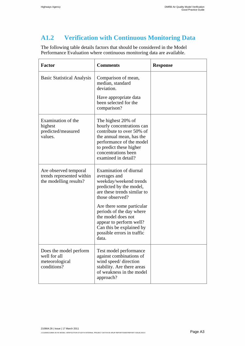
Highways Agency DMRB Air Quality Model Verification Good Practice Guide
210664.26 | Issue | 17 March 2011
J:\210000\210664-26 HA MODEL VERIFICATION STUDY\4 INTERNAL PROJECT DATA\4-05 ARUP REPORTS\0007REPORT ISSUE.DOCX Page A3
A1.2 Verification with Continuous Monitoring Data
The following table details factors that should be considered in the Model Performance Evaluation where continuous monitoring data are available.
Factor Comments Response
Basic Statistical Analysis Comparison of mean, median, standard deviation.
Have appropriate data been selected for the comparison?
Examination of the highest predicted/measured values.
The highest 20% of hourly concentrations can contribute to over 50% of the annual mean, has the performance of the model to predict these higher concentrations been examined in detail?
Are observed temporal trends represented within the modelling results?
Examination of diurnal averages and weekday/weekend trends predicted by the model, are these trends similar to those observed?
Are there some particular periods of the day where the model does not appear to perform well? Can this be explained by possible errors in traffic data.
Does the model perform well for all meteorological conditions?
Test model performance against combinations of wind speed/ direction stability. Are there areas of weakness in the model approach?

Highways Agency DMRB Air Quality Model Verification Good Practice Guide
210664.26 | Issue | 17 March 2011
J:\210000\210664-26 HA MODEL VERIFICATION STUDY\4 INTERNAL PROJECT DATA\4-05 ARUP REPORTS\0007REPORT ISSUE.DOCX Page A4
Testing of model performance against the same periods as the traffic modelling
Are there weaknesses in the model performance for different traffic modelling data (e.g. am and pm peaks). Are there any weaknesses owing to extrapolation of traffic data to different time periods?
5.4.1 Acceptability of Model Adjustment Factors
Examine model adjustment factors found in the Model Performance Evaluation, do these demonstrate that there us reasonable confidence in the modelling undertaken? Where adjustment factors are greater than five, consider whether alternative assessment methods are required to provide more confidence in the results.