i

DNA fingerprinting and genetic relationships among willow

(Salix spp.)

A Thesis Submitted to the College of

Graduate Studies and Research

In Partial Fulfillment of the Requirements

For the Degree of Master of Science

In the Department of Plant Sciences

University of Saskatchewan

Saskatoon

By

ALAIN CLAUDE NGANTCHA

© Copyright Alain Claude Ngantcha, March 2010. All rights reserved

i

PERMISSION TO USE

In presenting this thesis in partial fulfillment of the requirements for a Master of Science

degree from the University of Saskatchewan, I agree that the Libraries of this University may

make it freely available for inspection. I further agree that permission for copying of this thesis

in any manner, in whole or in part, for scholarly purposes may be granted by the professor or

professors who supervised my thesis work or, in their absence, by the Head of the Department or

the Dean of the College in which my thesis work was done. It is understood that any copying or

publication or use of this thesis or parts thereof for financial gain shall not be allowed without

my written permission. It is also understood that due recognition shall be given to me and to the

University of Saskatchewan in any scholarly use which may be made of any material in my

thesis.

Requests for permission to copy or to make other use of material in this thesis in whole or

part should be addressed to:

Head of the Department of Plant Sciences

College of Agriculture and Bioresources

University of Saskatchewan

Saskatoon, Saskatchewan S7N 5A8

ii

ABSTRACT

Given that morphological identification of willow is difficult, willow lines being

investigated for their suitability for use as short rotation crops for biomass production in

Saskatchewan were investigated with various molecular techniques as possible tools for DNA

fingerprinting. Flow cytometry was used to assess variation in nuclear DNA content and thus

ploidy level of the lines of the five species (Salix purpurea, Salix eriocephala, Salix

sachalinensis, and Salix dasyclados) and three hybrids (S. purpurea x S. miyabeana, S.

sachalinensis x S. miyabeana, S. viminalis x S. miyabeana). The DNA content varied between

1.14 and 3.00pg. Ploidy levels of the species varied from triploid to hexaploid while all hybrids

were tetraploid. RAPD and ISSR marker systems were used to assess genetic and taxonomic

relationships among all willow lines. Of 90 RAPD primers tested, 60 were selected and 99

polymorphic bands scored. Of 35 ISSR primers tested, 19 were selected and 35 polymorphic

bands scored. Both RAPD and ISSR dendrograms clustered together lines belonging to the same

species and same hybrid combination. A combination of strong and reproducible RAPD and

ISSR bands was used to develop identification keys for lines belonging to the same species.

The ribosomal RNA gene region, including the entire 5.8S RNA gene and the internal

transcribed spacers (ITS1 and ITS2) was amplified and sequenced to assess sequence homology

between the five species. The total length of the amplified region was 601bp, with the ITS1, 5.8

S and ITS2 being 223, 163, and 215bp respectively. Intra- and inter-species SNPs were observed,

6 within ITS1, and 3 within ITS2. No polymorphisms were found in the 5.8S gene. The low rate

of variation within the sequenced ITS fragment between species supports the monophyly of the

five species involved in this study, and confirms their belonging to the subgenus Caprisalix.

SCAR primers were designed from species-specific polymorphic nucleotides and applied to the

willow collection to test their use for species identification. A species identification key based on

SNPs is proposed.

iii

ACKNOWLEDGEMENTS

I am heartily thankful to my supervisor, Dr Graham Scoles, whose guidance,

encouragement, and support from the initial to the final level enabled me to develop an

understanding of this subject. I have fully benefited from his unfailing financial assistance

throughout my two years program.

I would like to extend my thanks to my committee, Dr Fu Yong-Bi, Dr Chen Gang, Dr

Tom Warkentin, Dr Bruce Coulman and Dr Kirstin Bett for their assistance, and advices.

I owe my deepest gratitude to Peter Eckstein, Aaron Beattie and Donna Hay of the crop

molecular genetics laboratory. This work couldn’t have been possible without their technical

support, advises and above all their heart-warming friendship.

I gratefully acknowledge Dr Ken Van Rees and his grad students Ryan Hangs, Sheala

Konecsni and Christine Stadnyk for the collaboration and team work. It was a great honour for

me to contribute in the willow project.

Thank you to my family, my mother, my brothers, my sisters, my uncles and my aunts for

the moral support and constant encouragements through tough times.

I am indebted to my Canadian family (Laurette, Eric Lefol and children) for the love care

and affection towards me since my arrival in Saskatoon.

Finally thank you to everybody who has contributed directly or indirectly to the

completion of this work.

iv

A tonton Lucien,

trouve en ce travail un motif de fierté, merci d’avoir

toujours cru en moi.

In memoriam.

A mon père,

reçois papa, mes remerciements pour m’avoir montré de

ton vivant les vertus du travail.

A Guillaume-Bertin mon frère, mon modèle, à Line et

Carine mes sœurs, je vous aime et je ne vous oublierais

jamais.

Ce travail vous est dédié, reposez en paix.

v

TABLE OF CONTENTS

PERMISSION TO USE i

ABSTRACT ii

ACKNOWLEDGEMENTS iii

ACKNOWLEDGEMENTS iv

TABLE OF CONTENTS v

LIST OF FIGURES viii

LIST OF TABLES xi

LIST OF APPENDICES xii

LIST OF ABREVIATIONS xiii

1-INTRODUCTION 1

2-LITERATURE REVIEW 2

2-1 Climate change 2

2-2 Biomass, a valuable source of renewable energy 3

2-2-1 Energy production from biomass 4

2-2-2 Willow, a dedicated crop for biomass and renewable

energy production 5

2-2-3 Other uses of willow 7

2-3 The genus Salix 8

2-3-1 Origin and distribution 8

2-3-2 Description and current classification 8

2-3-3 Ploidy variation in Salix species 11

2-3-4 Molecular genetics of the genus Salix 11

2-4 Genetic markers and fingerprinting 12

2-4-1 DNA markers and fingerprinting 13

2-4-2 Ribosomal RNA genes for phylogenetic analysis and fingerprinting 16

vi

2-4-2-1 Structural organization of ribosomal RNA genes 17

2-5 Measuring ploidy level 18

2-6 Methods of construction of dendrograms 18

3-THE USE OF FLOW CYTOMETRY, RAPD AND ISSR MARKERS FOR

FINGERPRINTING AND GENETIC DIVERSITY ANALYSIS OF Salix SPECIES 20

3-1 Abstract 20

3-2 Introduction 21

3-3 Materials and methods 23

3-3-1 Plant material 23

3-3-2 Flow cytometry 24

3-3-3 DNA extractions 24

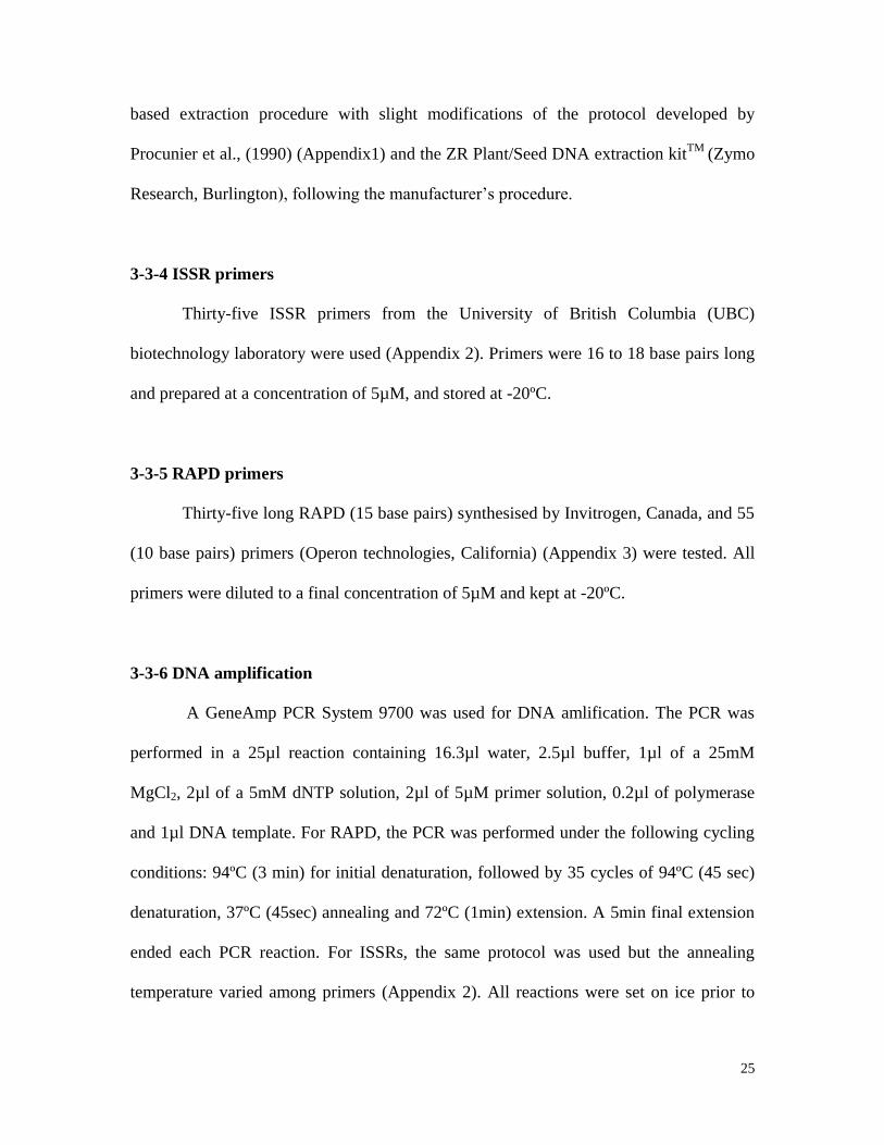
3-3-4 ISSR primers 25

3-3-5 RAPD primers 25

3-3-6 DNA amplification 25

3-3-7 Separation of amplified fragments 26

3-3-8 Scoring and data analysis 26

3-4 Results 27

3-4-1 DNA extraction 27

3-4-2 Flow cytometry 27

3-4-3 ISSR analysis 28

3-4-4 RAPD analysis 31

3-5 Discussion and conclusion 34

3-5-1 Markers for specific lines 37

4-THE USE OF 18-5.8-28S ITS OF rRNA GENES FOR FINGERPRINTING AND

PHYLOGENETIC ANALYSIS OF Salix SPECIES 41

4-1 Abstract 41

4-2 Introduction 42

4-3 Materials and methods 43

4-3-1 Plant material 43

vii

4-3-2 Primer design 43

4-3-3 DNA extraction 44

4-3-4 DNA amplification and gel electrophoresis 44

4-3-5 Cloning and sequencing 45

4-3-6 Species-specific SCAR markers 46

4-4 Results 47

4-4-1 Sequence alignment and nucleotide polymorphisms 48

4-4-1-1 Intra-clonal SNPs 48

4-4-1-2 Inter-specific SNPs 54

4-4-2 Species specific SCAR markers 55

4-5 Discussion and conclusions 65

5- GENERAL DISCUSSION AND CONCLUSION 68

6- NEXT STEPS 72

7- REFERENCES 73

8- APPENDICES 82

viii

LIST OF FIGURES

Figure 2.1 Cycle of biomass energy (Miyamoto, 2009) 4

Figure 2.2 Structure of the 18S-5.8S- 28S rRNA gene repeats 17

Figure 2.3 Structure of the 5S rRNA gene repeats 17

Figure 3.1 Banding patterns produced by PCR amplification of willow

lines with primer ISSR 825. Line Onondata (20) did not

produce any bands. 28

Figure 3.2 Banding pattern produced by PCR amplification of willow

lines with primer ISSR 834. 29

Figure 3.3 Banding pattern produced by PCR amplification of willow

lines with primer ISSR 843. Lines 9837-77 (23) and SVI (30)

did not produce any bands. 29

Figure 3.4 Dendrogram illustrating genetic similarities among

investigated willow species and hybrid lines generated

by UPGMA cluster analysis estimated from 35 ISSR

polymorphic bands produced by 19 ISSR primers.The lines

Hotel, 00X-026-082 and S. viminalis were not

included in this experiment 30

Figure 3.5 Banding patterns produced by PCR amplification of willow

lines with RAPD primer CMG. (Lines SX61 (31) and

Charly (34) did not produce bands 32

Figure 3.6 Dendrogram illustrating genetic similarities between

willow species and hybrids generated by UPGMA

cluster analysis (NTSYS PC v2.2) calculated from

99 RAPD markers produced by 60 RAPD primers 33

Figure 3.7 Band 500bp identifies hybrid lines S. viminalis x S. miyaneana

from other hybrid lines used in the program 37

Figure 4.1 Approximate location of primers for the amplification of

ITS regions 43

ix

Figure 4.2 PCR amplification of the ITS1-5.8S-ITS2 DNA

region produced monomorphic bands. 47

Figure 4.3 16 clones of segment of ITS fragment showing

intra-clonal SNPs in S. dasyclados 49

Figure 4.4 15 clones of segment of ITS fragment showing

intra-clonal SNPs in S. sachalinensis 49

Figure 4.5 ITS1 sequence alignments of consensus fragments of

S. eriocephala, S. purpurea, S. miyabeana and the

2 consensuses for S. dasyclados and S. sachalinensis

in the 1 to 223 base sequence 51

Figure 4.6 5.8S sequence alignments of consensus fragments of

S. eriocephala, S. purpurea, S. miyabeana and the

2 consensuses for S. dasyclados and S. Sachalinensis

in the 224 to 386 base sequence 52

Figure 4.7 ITS2 sequence alignments of consensus fragments of

S. eriocephala, S. purpurea, S. miyabeana and the

2 consensuses for S. dasyclados and S. sachalinensis

in the 387 to 601 base sequence 53

Figure 4.8 PCR amplification with forward primer

AAGGATCATTGTCGAAG produced a SCAR marker for

S. purpurea at 64ºC annealing temperature 55

Figure 4.9 PCR amplification with forward primer

GCATGACAAGCTGGGCC produced a SCAR marker for

S. eriocephala at 70ºC annealing temperature 56

Figure 4.10 PCR amplification with forward primer

GGAGCACGCCCTCTA produced a SCAR marker for

S. sachalinensis at 68ºC annealing temperature 57

Figure 4.11 PCR amplification with forward primer

ATTGAGTACTAGGAGCC did not produce the expected

430bp SCAR marker for S. dasyclados 58

Figure 4.12 Optimal SCAR marker for S.purpurea lines, hybrids lines of

S. purpurea x S. miyabeana and the line Hotel (64ºC annealing) 59

Figure 4.13 SCAR marker for S. sachalinensis, hybrids S. sachalinensis x S.

miyabeana and line SVI (68ºC annealing) 60

x

Figure 4.14 SCAR marker for S. eriocephala, Juliet and

Oneonta (70ºC annealing) 61

Figure 4.15 S. purpurea SCAR marker at 62ºC 62

Figure 4.16 S. purpurea SCAR marker at 63ºC 62

Figure 4.17 S. purpurea SCAR marker at 64ºC 62

Figure 4.18 S. sachalinensis SCAR marker (67ºC annealing) 63

Figure 4.19 S. sachalinensis SCAR marker (68ºC annealing) 63

Figure 4.20 S. eriocephala SCAR marker (67ºC annealing) 64

Figure 4.21 S. eriocephala SCAR marker (70ºC annealing) 64

Figure 4.22 Species identification key based on combination of ITS1

and ITS2 polymorphic nucleotides 67

Figure 5.1 Illustration of annealing sites of the reverse

primer CCGCCTGACCTGGGGT which led to the production

of two band sizes of 624bp and 432bp respectively, specific to

S. purpurea and hybrid lines S. purpurea x S. miyabeana. 69

xi

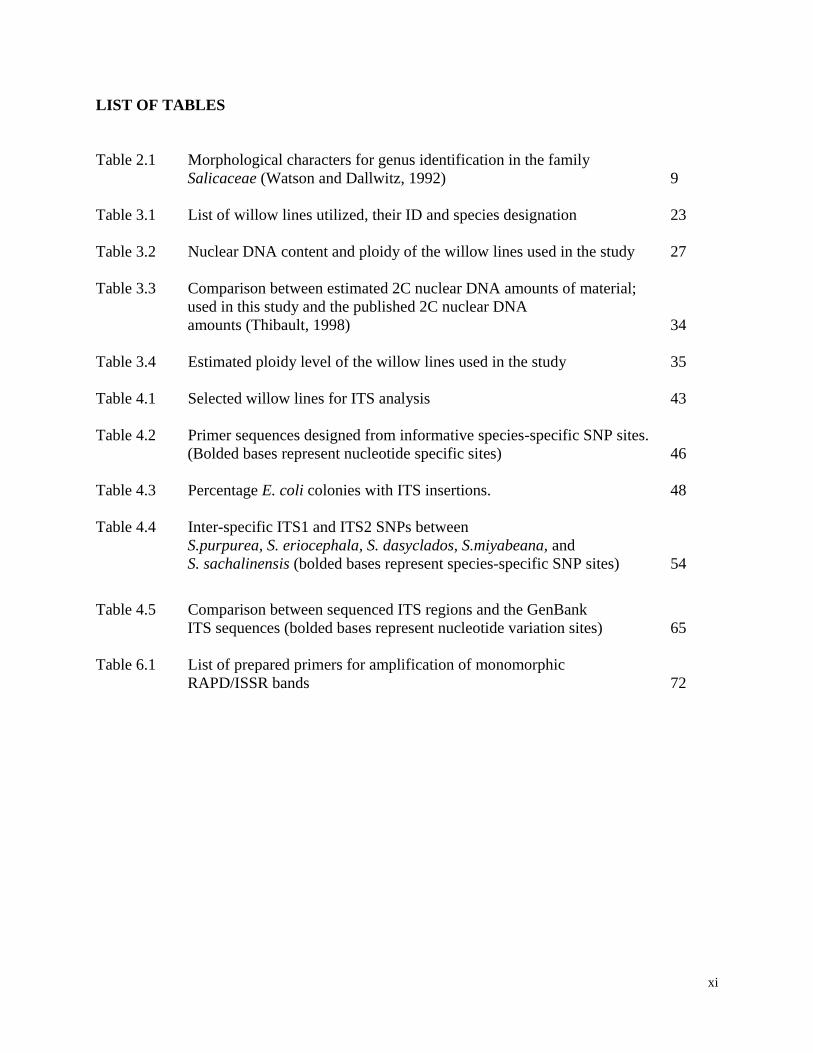
LIST OF TABLES

Table 2.1 Morphological characters for genus identification in the family

Salicaceae (Watson and Dallwitz, 1992) 9

Table 3.1 List of willow lines utilized, their ID and species designation 23

Table 3.2 Nuclear DNA content and ploidy of the willow lines used in the study 27

Table 3.3 Comparison between estimated 2C nuclear DNA amounts of material;

used in this study and the published 2C nuclear DNA

amounts (Thibault, 1998) 34

Table 3.4 Estimated ploidy level of the willow lines used in the study 35

Table 4.1 Selected willow lines for ITS analysis 43

Table 4.2 Primer sequences designed from informative species-specific SNP sites.

(Bolded bases represent nucleotide specific sites) 46

Table 4.3 Percentage E. coli colonies with ITS insertions. 48

Table 4.4 Inter-specific ITS1 and ITS2 SNPs between

S.purpurea, S. eriocephala, S. dasyclados, S.miyabeana, and

S. sachalinensis (bolded bases represent species-specific SNP sites) 54

Table 4.5 Comparison between sequenced ITS regions and the GenBank

ITS sequences (bolded bases represent nucleotide variation sites) 65

Table 6.1 List of prepared primers for amplification of monomorphic

RAPD/ISSR bands 72

xii

LIST OF APPENDICES

Appendix1 CTAB DNA extraction protocol 82

Appendix2 List of ISSR primer sequences and annealing temperatures 84

Appendix3 List of RAPD primer sequences 85

xiii

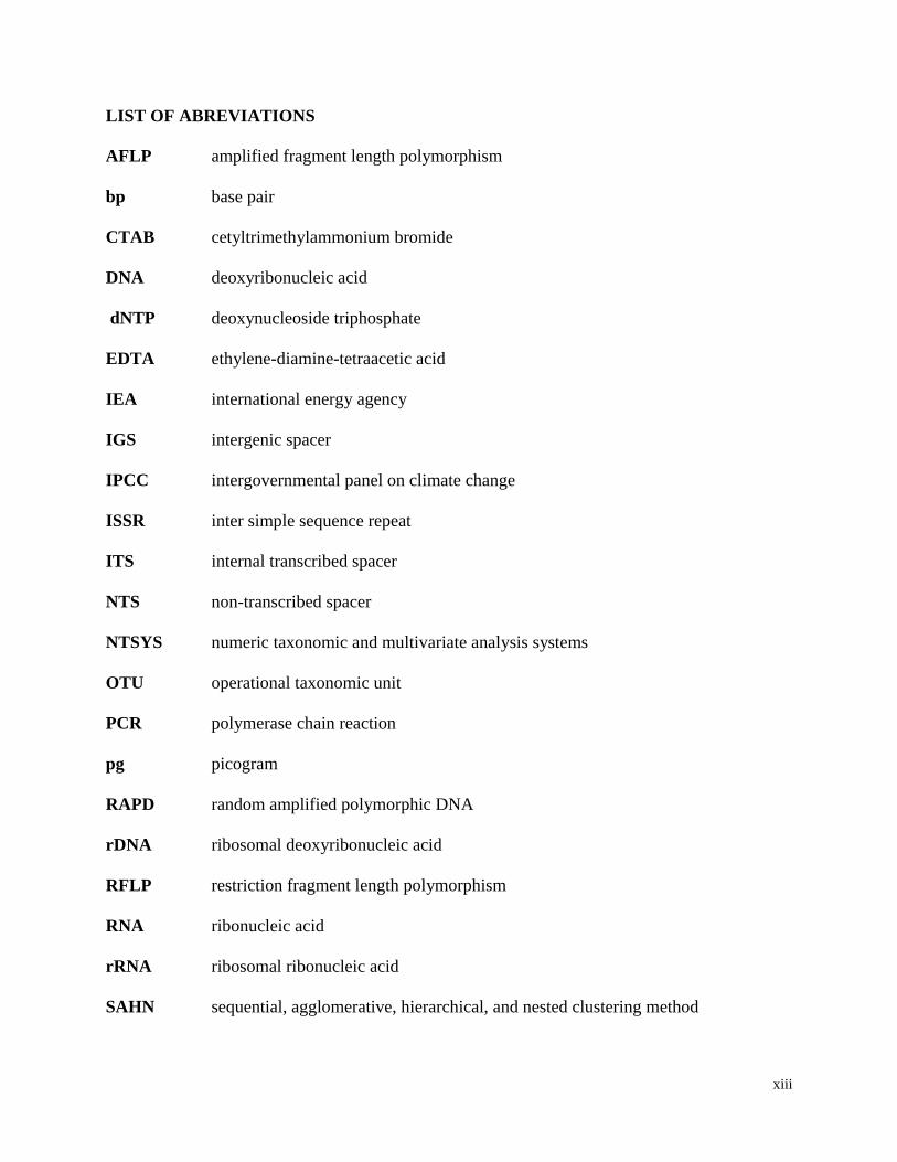
LIST OF ABREVIATIONS

AFLP amplified fragment length polymorphism

bp base pair

CTAB cetyltrimethylammonium bromide

DNA deoxyribonucleic acid

dNTP deoxynucleoside triphosphate

EDTA ethylene-diamine-tetraacetic acid

IEA international energy agency

IGS intergenic spacer

IPCC intergovernmental panel on climate change

ISSR inter simple sequence repeat

ITS internal transcribed spacer

NTS non-transcribed spacer

NTSYS numeric taxonomic and multivariate analysis systems

OTU operational taxonomic unit

PCR polymerase chain reaction

pg picogram

RAPD random amplified polymorphic DNA

rDNA ribosomal deoxyribonucleic acid

RFLP restriction fragment length polymorphism

RNA ribonucleic acid

rRNA ribosomal ribonucleic acid

SAHN sequential, agglomerative, hierarchical, and nested clustering method

xiv

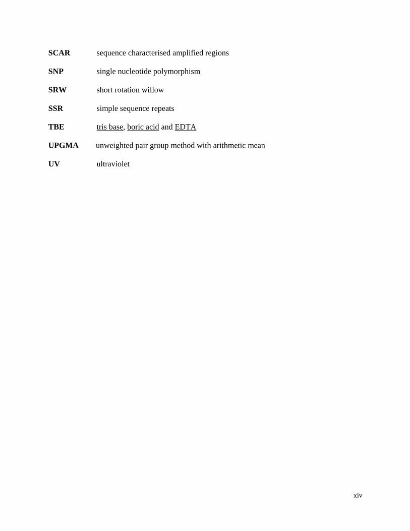
SCAR sequence characterised amplified regions

SNP single nucleotide polymorphism

SRW short rotation willow

SSR simple sequence repeats

TBE tris base, boric acid and EDTA

UPGMA unweighted pair group method with arithmetic mean

UV ultraviolet

1

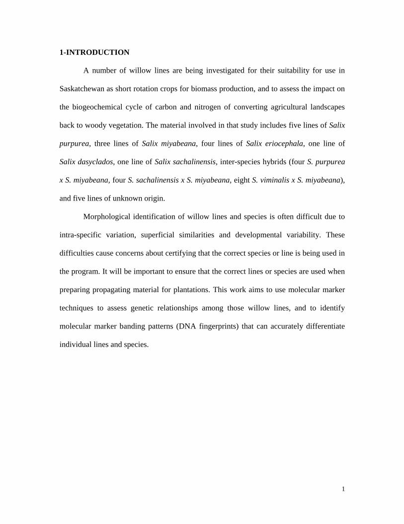
1-INTRODUCTION

A number of willow lines are being investigated for their suitability for use in

Saskatchewan as short rotation crops for biomass production, and to assess the impact on

the biogeochemical cycle of carbon and nitrogen of converting agricultural landscapes

back to woody vegetation. The material involved in that study includes five lines of Salix

purpurea, three lines of Salix miyabeana, four lines of Salix eriocephala, one line of

Salix dasyclados, one line of Salix sachalinensis, inter-species hybrids (four S. purpurea

x S. miyabeana, four S. sachalinensis x S. miyabeana, eight S. viminalis x S. miyabeana),

and five lines of unknown origin.

Morphological identification of willow lines and species is often difficult due to

intra-specific variation, superficial similarities and developmental variability. These

difficulties cause concerns about certifying that the correct species or line is being used in

the program. It will be important to ensure that the correct lines or species are used when

preparing propagating material for plantations. This work aims to use molecular marker

techniques to assess genetic relationships among those willow lines, and to identify

molecular marker banding patterns (DNA fingerprints) that can accurately differentiate

individual lines and species.

2

2-LITERATURE REVIEW

2-1 Climate change

For more than one century, modern societies have been deeply dependent on

fossil carbon for fuel production and for chemicals ranging from plastic polymers to

drugs and food additives (Benning and Pichersky, 2008). Oil production has increased

from less than 1 million tonnes a year in 1870, to more than 3 billion tonnes a year

(Bennewitz, 2009). These industrial activities have caused important releases of harmful

organic and inorganic compounds to the environment, including greenhouse-effect gases,

heavy metals, and petroleum hydrocarbons (Wilcke and Amelung, 2000; Huang et al.,

2005; Rodríguez et al., 2008;). Since the Industrial Revolution, atmospheric carbon

dioxide concentration has risen from 280 to 365 ppm, and predictions are that it could

reach 700 ppm by the second half of the 21st century (Houghton et al., 1996; Lamlom

and Savidge, 2003). The CO2 layer helps to retain heat that would otherwise be lost to

space. An increase of atmospheric carbon dioxide concentration consequently leads to

global warming (Bennewitz, 2009).

In addition, forest ecosystems are continuously destroyed releasing CO2. Between

1990 and 1997, 5.8 ± 1.4 million hectares of the world’s humid tropical forest were lost

each year, with a further 2.3 ± 0.7 million hectares of forest visibly degraded (Achard et

al., 2002). In Canada, the main causes of deforestation are the conversion of forest to

agricultural and urban lands. The deforestation rate in Canada is estimated at 546-805

km2 per year linked with a yearly release of 9.5-14.0 Mt carbon dioxide (Robinson et al.,

1999). The combined effect of forest loss and intensive use of fossil fuel leads to an

3

increase of atmospheric carbon dioxide concentration and global warming (Benning and

Pichersky, 2008; IEA, 2002), which is the main threat to human development and the

future of the planet (Houghton et al., 1996). The Intergovernmental Panel on Climate

Change (IPCC) predicts an anthropogenic warming increase between 1.4 and 5.8°C over

the 21st

century (IPCC, 2001). In Canada, the annual mean temperature increased by

1.2°C between 1955 and 2005 (Vincent et al., 2007).

Many countries including Canada have ratified international agreements such as

the Kyoto protocol to reduce greenhouse gas emissions and mitigate human impact on

global warming. Those agreements rely on the identification of renewable sources of

energy that can substitute for the use of fossil fuel energy (reducing fossil fuel carbon

dioxide emissions to the atmosphere), as well as the adoption of sustainable

environmental management practices (Smart et al., 2005; IEA, 2002).

2-2 Biomass, a valuable source of renewable energy

Concerns about global warming, air and water pollution associated with the use of

fossil fuels, have brought growing interests in the development of bio-energy and bio-

products in western countries (Keoleian and Volk, 2005). Global energy-use projections

predict that biomass has the potential to become one of the major primary energy sources

in the coming decades and modernized bio-energy systems are suggested to be important

contributors to future sustainable energy systems in both industrialized and developing

countries (IEA, 2002; Berndes et al., 2003).

Biomass energy is unique among renewable energy sources (wind, water and

solar energy) in that it can be both a source of electricity, and a source of liquid and

4

gaseous fuels (Graham et al., 1992). Renewable biomass feedstock can come from

various sources including forest, agricultural crops and short rotation woody crops

(Abrahamson et al., 1998; Volk et al., 2004). Short rotation woody crops show multiple

environmental and rural development benefits, and are promoted as a potential source of

significant amounts of renewable biomass that could offer landowners an attractive

alternative use for marginal croplands (Berndes et al., 2003).

2-2-1 Energy production from biomass

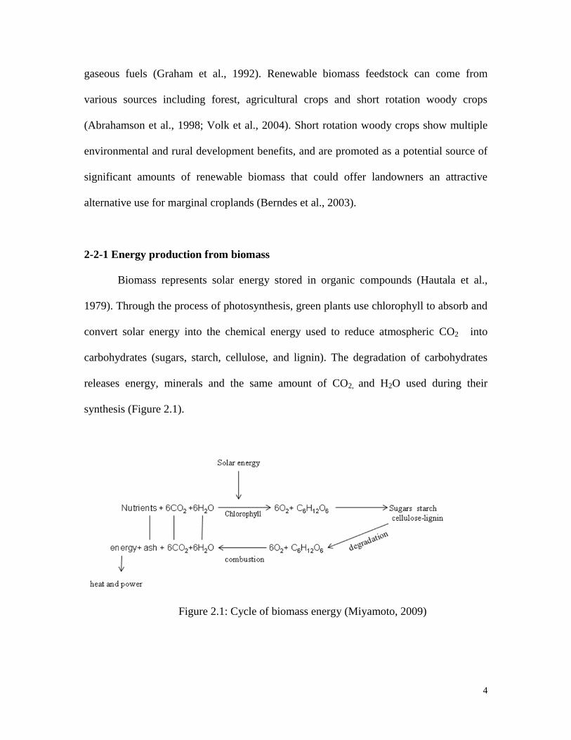
Biomass represents solar energy stored in organic compounds (Hautala et al.,

1979). Through the process of photosynthesis, green plants use chlorophyll to absorb and

convert solar energy into the chemical energy used to reduce atmospheric CO2 into

carbohydrates (sugars, starch, cellulose, and lignin). The degradation of carbohydrates

releases energy, minerals and the same amount of CO2, and H2O used during their

synthesis (Figure 2.1).

Figure 2.1: Cycle of biomass energy (Miyamoto, 2009)

5

Many technologies can be used to generate energy and power from woody

biomass. Direct combustion technologies can be used to convert biomass fuels into

various forms of energy (mechanical energy, heat or electricity), using processes similar

to that employed for fossil fuels (Dumbleton, 1997). The process involves the burning of

biomass in a furnace or a boiler to generate heat and steam. Steam can then run through a

turbine to produce mechanical energy. If the turbine is connected to an electrical

generator it produces electricity.

Gasification technology uses high temperature and high pressure for partial

oxidation of biomass into combustible gas (Nordin and Kjellström, 1996). The gas fuel

resulting from this process consists mainly of carbon monoxide and hydrogen with small

amounts of methane, ethane and ethylene (Dumbleton, 1997).

Pyrolysis is the process where biomass is combusted at high temperatures and

decomposed in the absence of oxygen. It results in the production of solid, liquid and

gaseous products. Pyrolysis oil can be combusted in engines to produce heat and power

(Bidini et al., 2003).

Research is also underway to develop bacterial and yeast strains that can be used

for bio-ethanol production from lignocellulosic sugars (Zaldivar et al., 2001).

2-2-2 Willow, a dedicated crop for biomass and renewable energy production

Woody biomass crop development in northern temperate areas has focused on

willow shrubs and poplar (Abrahamson et al., 1998; Perttu, 1999; Keoleian and Volk,

2005). Willow, however, exhibits more diversity (number of species) and grows in a

wider range of environments compared to poplar (Verwijst, 2001).

6

Most willows are characterised by particular physiological assets that make them

suitable for biomass and energy production (Kuzovkina and Quigley, 2005). Willows

exhibit high growth rates and biomass productivity (Keoleian and Volk, 2005). The

growth rate of willow is superior to most cool temperate tree species, with an annual

growth of 1 to 4 m during the first five years after planting, depending on soil fertility and

moisture regimes (Wilkinson, 1999). Willow is considered among the most promising

biomass fuels in many temperate regions. In Quebec, Labrecque and Teodorescu, (2003)

reported 71.3 tonnes of dry matter yield per hectare three years after planting. Willow

plantations are clonally propagated and can be harvested every three to five years, after

which the cut stools regenerate 5-14 new stems to provide another harvest, and may

continue to do so up to eight times, giving a productive lifespan of 20-32 years (Volk et

al., 2004). This provides farmers with a new crop that produces a regular income and

faster returns than those associated with conventional forestry (Volk et al., 2004).

Energy produced from short rotation willow (SRW) biomass is renewable,

because the growth of new plants and trees replenishes the supply. Carbon dioxide

emission from burning of SRW biomass is neutral, because it is recycled via

photosynthesis in stands growing to replace those harvested (IEA, 2002). Carbon

sequestration in the soil increases in SRW plantations, and net emissions of carbon

dioxide may even be negative (Grogan and Matthew, 2002).

7

2-2-3 Other uses of willow

Willow plantations can be used as a biological filter for wastewater treatment via

a system based on soil filtration of effluents, the degradation of organic particles by

micro-organisms, and the uptake of nutrients and heavy metals by willow trees (Pulford

and Watson, 2003). The bio-filtration system offers many advantages including recycling

of nutrients, a less expensive purification system for water companies, and higher

profitability for willow growers due to a lower cost for fertilisers and a higher yield. The

use of such willow as wood fuel would allow heavy metal recovery through the scrubbing

of smoke gases and proper handling of ashes (Pulford and Watson, 2003).

Willows possess the major requirements for plant survival in degraded

ecosystems including the ease of vegetative propagation, the ability to re-establish from

cut stumps and produce a dense coppice (Volk et al., 2004), and the ability to accumulate

high levels of toxic metals (Perttu, 1999; Mirck et al., 2005). Willows are recommended

for remediation of oil-mining areas because of their potential to rapidly sequester

pollutants and re-establish green cover (Kuzovkina and Quigley, 2005). The colonization

of environmentally disturbed sites by willow species supports the establishment of

pioneer species, fasters the recovery of damaged ecosystems and the re-establishment of

natural ecological complexity (Kuzovkina and Quigley, 2005). Many invertebrates, birds

and animals feed on willow and support a large food chain for higher trophic level

organisms (Kennedy and Southwood, 1984). Willow energy plantations can create new

habitat opportunities for wildlife in degraded ecosystems (Kuzovkina and Quigley, 2005).

8

2-3 The genus Salix

2-3-1 Origin and distribution

Plants belonging to the genus Salix are among the earliest recorded pre-ice age

flowering plants (Newsholme, 2002). The genus Salix originally arose in the subtropics,

and then advanced slightly into the tropics, expanded into the temperate regions, and later

into the Artic. Salix species are now mostly distributed in the northern temperate zones

(Europe, Asia, North America). Species diversity is richest in China (270 species) and

Russia (120 species). There are about 65 species in Europe and 160 species in North

America (Kuzovkina and Quigley, 2005). Only 3 species are native to central and South

America (Argus, 1986). In tropical Africa, there are about 12 species most of which are

endemic only to Africa and are extremely local (Newsholme, 2002).

2-3-2 Description and current classification

The genus Salix belongs to the family Salicaceae. Members of this family are

trees and shrubs (Watson and Dallwitz, 1992). Flowers are aggregated in inflorescences

called catkins which are usually pendulous or erect (Dorn, 1976). Originally, Linnaeus

(1763) described and divided this family into two genera, the genus Populus and the

genus Salix. Nakai (1920) described a new genus Chosenia, which bears intermediate

characters between these genera (Table 2.1).

9

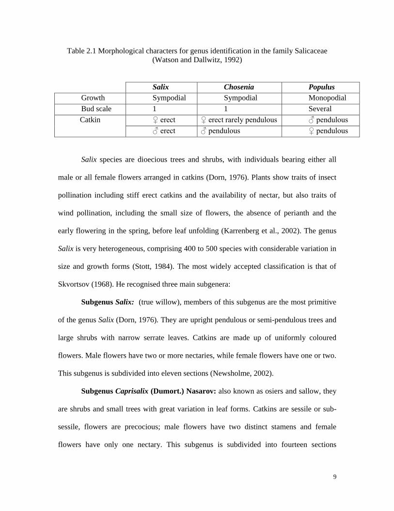
Table 2.1 Morphological characters for genus identification in the family Salicaceae

(Watson and Dallwitz, 1992)

Salix Chosenia Populus

Growth Sympodial Sympodial Monopodial

Bud scale 1 1 Several

Catkin ♀ erect ♀ erect rarely pendulous ♂ pendulous

♂ erect ♂ pendulous ♀ pendulous

Salix species are dioecious trees and shrubs, with individuals bearing either all

male or all female flowers arranged in catkins (Dorn, 1976). Plants show traits of insect

pollination including stiff erect catkins and the availability of nectar, but also traits of

wind pollination, including the small size of flowers, the absence of perianth and the

early flowering in the spring, before leaf unfolding (Karrenberg et al., 2002). The genus

Salix is very heterogeneous, comprising 400 to 500 species with considerable variation in

size and growth forms (Stott, 1984). The most widely accepted classification is that of

Skvortsov (1968). He recognised three main subgenera:

Subgenus Salix: (true willow), members of this subgenus are the most primitive

of the genus Salix (Dorn, 1976). They are upright pendulous or semi-pendulous trees and

large shrubs with narrow serrate leaves. Catkins are made up of uniformly coloured

flowers. Male flowers have two or more nectaries, while female flowers have one or two.

This subgenus is subdivided into eleven sections (Newsholme, 2002).

Subgenus Caprisalix (Dumort.) Nasarov: also known as osiers and sallow, they

are shrubs and small trees with great variation in leaf forms. Catkins are sessile or sub-

sessile, flowers are precocious; male flowers have two distinct stamens and female

flowers have only one nectary. This subgenus is subdivided into fourteen sections

10

(Newsholme, 2002). Most willows used in crop systems belong to this subgenus. More

than 125 species are known worldwide (Volk et al., 2004).

Chamaetia (Dumort.) Nasarov: Plants are dwarf or procumbent shrubs of less

than 1m high, leaves are less than 10 cm long, Catkins are borne by leafy branchlets, and

male flowers have two stamens, occasionally one. This subgenus is subdivided into seven

sections (Newsholme, 2002).

The taxonomy of the genus Salix has been continuously under revision

(Skvortsov, 1968; Meikle, 1984). Many factors contribute to difficulties in the

identification of Salix species, including high morphological variability, widespread

hybridization and introgression, and variation in ploidy levels (Argus, 1997). Within the

genus Salix, quantitative characters like length of catkins, absence or presence of

flowering branchlets, and ovary length vary with developmental stage. Some structures

like stipules or floral bracts may be lost with maturity (Argus, 1986). In addition, the use

of floral characteristics for identification is limited because of the extremely reduced size

of the flowers (Argus, 1997).

Hybridisation is an important source of variability within the genus Salix (Dorn,

1976). Inter-specific crosses frequently occur in the wild and in cultivation. Hybrids may

be imperfectly intermediate or highly variable, resulting in an interpretation that

unrecognized hybrid plants are part of the morphological variation. Most hybrids are

fertile and can cross with other species and hybrids, bringing more problems associated

with classification and identification (Stott, 1984).

11

2-3-3 Ploidy variation in Salix species

Salix species are dioecious. Pollination is either entomophilous or anemophilous.

The basic chromosome number is 19. The ploidy level varies both between and within

members of the same species (Håkansson, 1955; Darlington and Wylie, 1961). The

chromosome number ranges from (2n=38) for diploids; (2n=57) for tripoids; (2n=76) for

tetraploids; (2n=95) for pentaploids; (2n=114) for hexaploids; to (2n=152) for octoploids

(Suda and Argus, 1968). Over 40% of Salix species are polyploids. Polyploidization may

have occurred independently several times in Salix (Dorn, 1976). The evaluation of

chromosome number and ploidy level can help to recognise the parentage of hybrids

involving species with different ploidy levels, and to delimit taxa unrecognised

morphologically (Suda and Argus, 1968; Chmelar, 1979).

2-3-4 Molecular genetics of the genus Salix

Research on the molecular genetics of Salix species is recent. Barker et al., (1999)

used random amplified polymorphic DNA (RAPD) and amplified fragment length

polymorphism (AFLP) analysis to characterise the genetic diversity in potential biomass

of willows. They reported that RAPD analysis can be performed with relatively crude

DNA, but differences in DNA purity between samples can be a cause of un-reproducible

profiles. Twenty RAPD primers were able to distinguish up to 10 of the 20 lines involved

in that study. The AFLP technique revealed more genetic diversity and was better able to

discriminate closely related lines. High quality DNA was essential for complete digestion

with the restriction enzymes required for AFLP. Hanley et al., (2002) used 291 AFLP and

39 microsatellite markers to develop the genetic linkage map of Salix viminalis. Barker et

12

al., (2003) developed microsatellites from an enriched library of Salix burjatica, most of

which cross-amplified diverse Salix species. Sulima et al., (2009) used RAPD to reveal

the genetic diversity and fingerprint lines of Salix purpurea. Nucleotide sequences of

ribosomal RNA gene regions (ITS1, 5.8S and ITS2) were used by Leskinen and Alstrom,

(1999) to study the molecular phylogeny of Salicaceae and closely related

Flacourtiaceae. They reported a low inter-specific variation in ITS sequence among

members of the family Salicaceae.

2-4 Genetic markers and fingerprinting

A genetic marker can be defined as a measurable character that can detect

variation in either the phenotype or the genotype (King and Stansfield, 1990). Genetic

markers can be based on visually assessable traits (morphological markers), on gene

products (biochemical markers), or rely on a DNA assay (DNA markers).

Morphological markers were very useful to early geneticists for the study of

classical heredity. However, their number is limited, and their expression can vary over a

range of environments or be influenced by pleiotropic interactions and developmental

stage (Staub et al., 1996).

Molecular markers are DNA sequences that reveal sites of variation in DNA.

DNA sequence variation generally arises from point mutations (substitutions)

rearrangements, insertions, deletions, and errors in replication (Paterson, 1996). They

provide a new supply of character differences that can be detected in laboratory assays.

There are two categories of molecular markers: Biochemical markers based on the

detection of differences in proteins through gel electrophoresis, and DNA markers based

13

on detection of variation in DNA (Winter and Kahl, 1995). Compared to morphological

and biochemical markers, DNA markers are more abundant, more polymorphic,

reproducible, discriminating and not subject to environmental changes; they can be

detected in any tissue of the organism at any developmental stage (Winter and Kahl,

1995).

2-4-1 DNA markers and fingerprinting

Many different DNA marker systems are now widely used. They are either

hybridization or polymerase chain reaction (PCR) based (Collard et al., 2005). The most

commonly known hybridization based DNA marker system is restriction fragment length

polymorphism (RFLP). This system is based on digestion of genomic DNA with

restriction enzymes. The resulting fragments are separated by gel electrophoresis, blotted

onto a filter, and probed with a small fragment of radio-labelled cloned genomic or

complementary DNA. Through autoradiography, probes can be visualized on the filter

and banding patterns used for genetic analysis (Beckmann and Soller, 1986). Genetic

variations come from gain or loss of restriction sites between genomes as a result of

mutations, insertions, inversions, or deletions (Doebley and Wendel, 1989). However,

RFLP marker systems have some limitations. The process is laborious, time consuming

and requires a relatively large amount of good quality DNA (Beckmann and Soller,

1986).

The invention of PCR in 1984 by Mulli, (1990) brought the development of new

marker technologies that were able to surmount some of the limitations of RFLP (Tautz

and Renz, 1984; Williams et al., 1990). The random amplified polymorphic DNA

14

technique (RAPD) is a PCR-based technique in which a single short oligonucleotide (10

bp) of arbitrary sequence anneals to the genomic DNA at different sites on

complementary strands of the DNA template. If the priming sites are within an

amplifiable range of each other, a discrete DNA product is formed through thermo-cyclic

amplification (Williams et al., 1990). Amplified fragments (within the 0.5-5 kb range)

can be separated by gel electrophoresis and visualised by UV light after staining with

ethidium bromide. The polymorphisms are identified as the presence or absence of a

given amplification product in the gel, and result from variation in the sequence of the

primer binding sites, or from chromosomal rearrangements within the amplified

sequence, altering the size or the successful amplification of the target site (Williams et

al., 1990). No prior sequence information is required for the design of RAPD primers and

they can easily be applied to any organism (Hadrys et al., 1992). The RAPD technique

has a wide range of applications, including genetic similarity analysis (Sulima et al.,

2009), fingerprinting (Castiglione et al., 1993), and genetic mapping (Hadrys et al.,

1992).

Microsatellites or simple sequence repeats (SSRs) are loci where di- tri- or tetra-

nucleotide sequences of DNA are repeated in tandem arrays (Powell et al., 1996). SSRs

are scattered throughout genomes and exhibit a higher mutation rate compared to other

regions of DNA, due to slipped strand mispairing (slippage) during DNA replication on a

single DNA strand (Jeffreys et al., 1985). The number of times the sequence is repeated

at a particular locus often varies between individuals, populations, and between species

(Jeffreys et al., 1985). The development of microsatellite markers involves several steps

including the development of a genomic DNA library, the identification of microsatellite

15

loci and the design of suitable forward and reverse primers for amplification (Semagn et

al., 2006).

Inter simple sequence repeats (ISSRs) are arbitrary multilocus markers produced

by PCR amplification of genomic DNA with single microsatellite based primers (Tautz

and Renz, 1984). The ISSR technique is a RAPD-like approach that accesses variation in

the numerous microsatellite regions dispersed throughout genomes (Joshi et al., 2000).

The primer locates two microsatellite regions within an amplifiable distance on the DNA

template strands, and the PCR reaction generates a band of a particular size representing

the stretch of DNA between the microsatellites (Semagn et al., 2006). ISSRs are highly

polymorphic, do not require prior genomic information for primer design, and show a

higher reproducibility than RAPD and RFLP approaches (Tsumura et al., 1996). ISSR

markers have been used to assess genetic diversity and to fingerprint many crops (maize,

beans, barley) (Kantety et al., 1995; Metals et al., 2000).

Amplified Fragment Length Polymorphism (AFLP) involves the digestion of

genomic DNA followed by ligation of adaptors to the ends of digested fragments, and the

selective PCR amplification of a set of fragments (Hanley et al., 2002). Amplified

fragments are separated on acrylamide gels and visualized by autoradiography, silver

staining or fluorescent sequencing equipment (Vos et al., 1995). AFLP is a multilocus

DNA profiling technique in which it is possible to obtain information for many different

loci in a single assay. AFLP produces a large amount of data from a single experiment,

and is a useful method for distinguishing between closely related individuals (Vos and

Kuiper, 1997). However, AFLP requires high quality DNA for complete digestion.

16

Single nucleotide polymorphisms (SNPs) are DNA sequence variations occurring

when a single nucleotide in the genome differs between members of a species. They can

occur in both coding and non-coding regions, and represent the largest set of sequence

variants in most organisms (Kwok et al., 1996). Specific oligonucleotide primers can be

designed from SNPs to develop sequence characterized amplified region (SCAR)

markers through PCR amplification of specific DNA fragments (McDermott et al., 1994).

The SNP marker approach requires prior sequence information and is increasingly used

as DNA sequences become accessible in databases (Kurt et al., 2005).

2-4-2 Ribosomal RNA genes in phylogenetic analysis and fingerprinting

Ribosomal RNA genes (rDNA) are DNA sequences responsible for the synthesis

of ribosomal RNA (rRNA) (Shiue et al., 2009). These genes are tandemly repeated along

chromosomes and exist in thousands of copies. Coding regions (18S, 5.8S, 5S, and 28S)

are highly conserved between families, genera and species. Non-coding regions, (the non

transcribed spacer (NTS), the intergenic spacer (IGS), and the internal transcribed spacer

(ITS)) are much more variable, but undergo rapid concerted evolution known as

molecular drive, that promotes intra-genomic uniformity (Leskinen and Alstrom, 1999).

The characterisation of spacers can be used for inter-species comparison, genetic

variations and phylogenetic relationships among taxa (Scoles et al., 1987; Shiue et al.,

2009).

17

2-4-2-1 Structural organization of ribosomal RNA genes

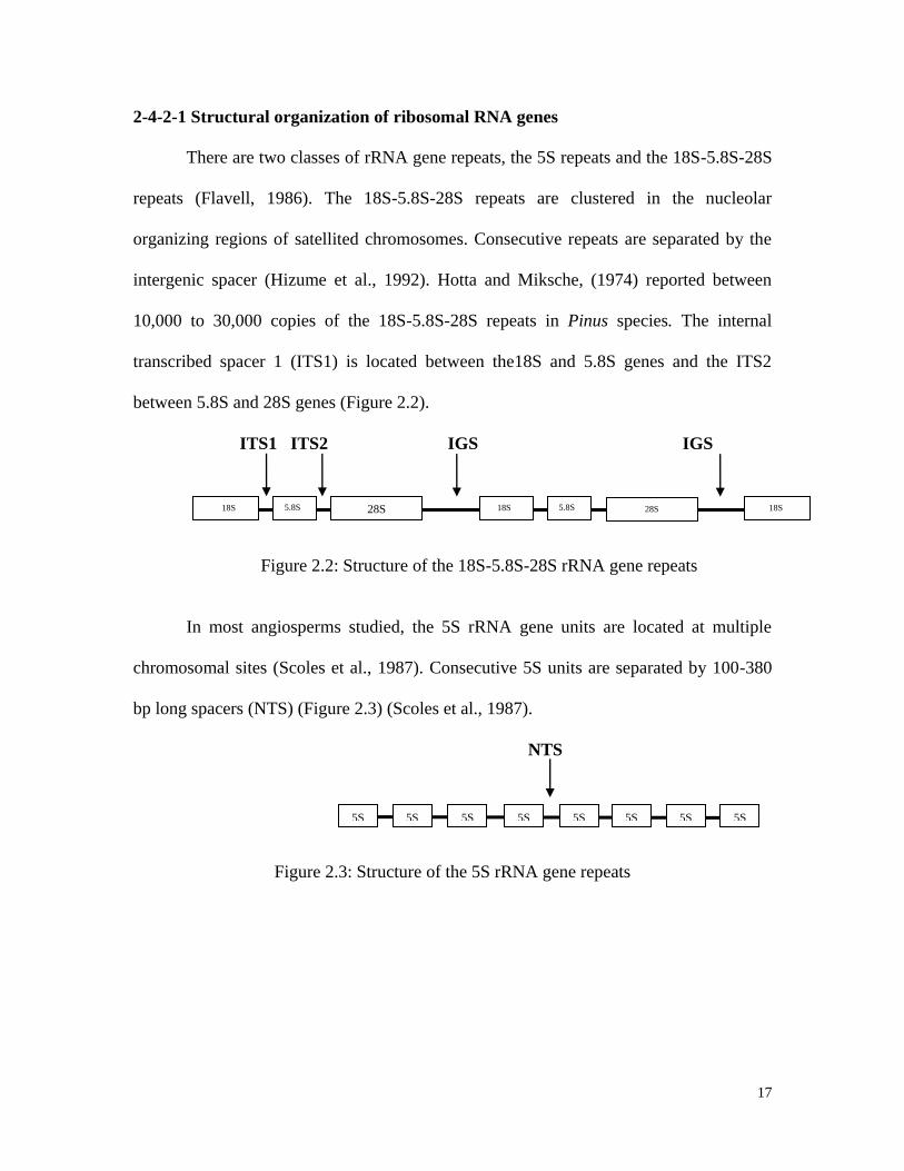
There are two classes of rRNA gene repeats, the 5S repeats and the 18S-5.8S-28S

repeats (Flavell, 1986). The 18S-5.8S-28S repeats are clustered in the nucleolar

organizing regions of satellited chromosomes. Consecutive repeats are separated by the

intergenic spacer (Hizume et al., 1992). Hotta and Miksche, (1974) reported between

10,000 to 30,000 copies of the 18S-5.8S-28S repeats in Pinus species. The internal

transcribed spacer 1 (ITS1) is located between the18S and 5.8S genes and the ITS2

between 5.8S and 28S genes (Figure 2.2).

ITS1 ITS2 IGS IGS

Figure 2.2: Structure of the 18S-5.8S-28S rRNA gene repeats

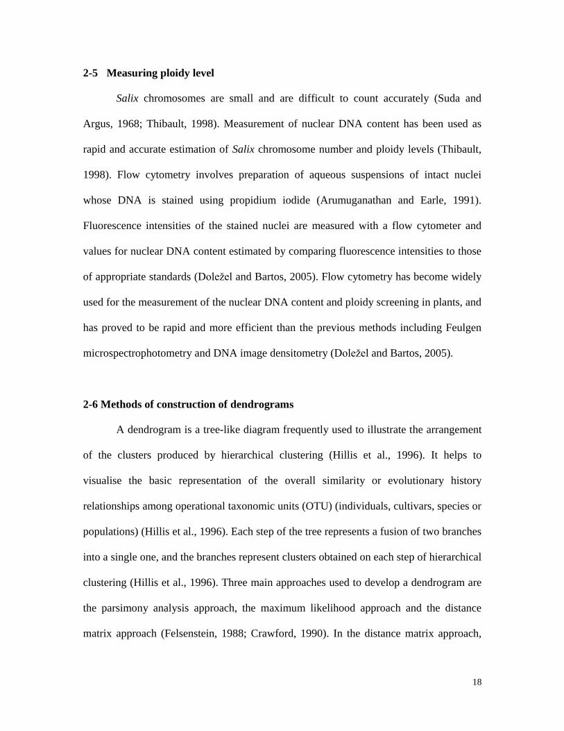
In most angiosperms studied, the 5S rRNA gene units are located at multiple

chromosomal sites (Scoles et al., 1987). Consecutive 5S units are separated by 100-380

bp long spacers (NTS) (Figure 2.3) (Scoles et al., 1987).

NTS

Figure 2.3: Structure of the 5S rRNA gene repeats

5S

5S

5S

5S

5S

5S

5S

5S

18S 5.8SS

28S 18S 5.8SSS

28S 18S

18

2-5 Measuring ploidy level

Salix chromosomes are small and are difficult to count accurately (Suda and

Argus, 1968; Thibault, 1998). Measurement of nuclear DNA content has been used as

rapid and accurate estimation of Salix chromosome number and ploidy levels (Thibault,

1998). Flow cytometry involves preparation of aqueous suspensions of intact nuclei

whose DNA is stained using propidium iodide (Arumuganathan and Earle, 1991).

Fluorescence intensities of the stained nuclei are measured with a flow cytometer and

values for nuclear DNA content estimated by comparing fluorescence intensities to those

of appropriate standards (Doležel and Bartos, 2005). Flow cytometry has become widely

used for the measurement of the nuclear DNA content and ploidy screening in plants, and

has proved to be rapid and more efficient than the previous methods including Feulgen

microspectrophotometry and DNA image densitometry (Doležel and Bartos, 2005).

2-6 Methods of construction of dendrograms

A dendrogram is a tree-like diagram frequently used to illustrate the arrangement

of the clusters produced by hierarchical clustering (Hillis et al., 1996). It helps to

visualise the basic representation of the overall similarity or evolutionary history

relationships among operational taxonomic units (OTU) (individuals, cultivars, species or

populations) (Hillis et al., 1996). Each step of the tree represents a fusion of two branches

into a single one, and the branches represent clusters obtained on each step of hierarchical

clustering (Hillis et al., 1996). Three main approaches used to develop a dendrogram are

the parsimony analysis approach, the maximum likelihood approach and the distance

matrix approach (Felsenstein, 1988; Crawford, 1990). In the distance matrix approach,

19

the tree is generated with an algorithm based on functional relationships among distance

values. Several methods are based on this approach, including the Wagner distance

method, the least square method, the neighbour joining method and the Unweighted Pair

Group Method with Arithmetic Mean (UPGMA). The UPGMA is known as the simplest

and the most frequently used method, especially for allelic frequency data (Crawford,

1990). It is based on a sequential algorithm that generates the tree in 2 steps. First, two

most similar OTU are identified and clustered in a single composite OTU, which will

then be grouped with the next most similar one.

20

3-THE USE OF FLOW CYTOMETRY, RAPD AND ISSR MARKERS FOR

FINGERPRINTING AND GENETIC DIVERSITY ANALYSIS OF Salix SPECIES

3-1 Abstract

Flow cytometry was used to assess variation in nuclear DNA content and ploidy

level of 35 willow lines. The DNA content varied between 1.14 and 3.00pg. There was

slight variation among lines of the same species. Ploidy levels of the species varied from

triploid to hexaploid. All hybrid lines came from crosses between tetraploid parents.

RAPD and ISSR marker systems were used to assess genetic and taxonomic

relationships among the willow lines. Of 90 RAPD primers tested, 60 were selected and

99 polymorphic bands were used for genetic relationships analysis. Thirty five ISSR

primers were tested, 19 produced polymorphic bands and a total of 35 polymorphic bands

were used for genetic relationships analysis. Both RAPD and ISSR dendrograms

clustered together lines belonging to the same species. Hybrid lines were grouped

together. Both dendrograms clustered the line Juliet with lines of S. eriocephala, Hotel

with lines of S. purpurea and India with lines of S. dasyclados. The 2C nuclear DNA

values of Juliet and Hotel also fell within the range of 2C nuclear DNA values of S.

eriocephala and S. purpurea lines respectively. A combination of strong and reproducible

RAPD and ISSR bands were used to develop identification keys for lines belonging to the

same species. These results show that RAPD, ISSR marker techniques and flow

cytometry can be efficiently used to discriminate among closely related willow lines.

21

3-2 Introduction

Biomass willow lines are being investigated for their suitability as short rotation

biomass energy crops in Saskatchewan. Willow lines being used in that investigation can

be grouped into five species (Salix purpurea, Salix miyabeana, Salix eriocephala, Salix

dasyclados, Salix sachalinensis) and inter-species hybrids (S. purpurea x S. miyabeana,

S. sachalinensis x S. miyabeana, S. viminalis x S. miyabeana) (Table 3.1), all belonging

to the subgenus Caprisalix. Observation of this material in the field showed that different

lines of the same species tend to be very similar morphologically. Inter-specific hybrids

bear intermediate characters between parents, but exhibit morphological variability.

Some hybrids can easily be misidentified as parents. Because of their unknown origin,

five lines included in this investigation could not be accurately classified.

The genus Salix is known to be one of the few woody genera with a large number

of polyploid taxa (Suda and Argus, 1968; Chmelar, 1979). The evaluation of ploidy level

can therefore be useful to delimit taxa and to recognise the parentage of hybrid crosses

involving species with different ploidy levels (Chmelar, 1979). Ploidy levels can be

deduced from nuclear DNA values measured with flow cytometry (Morgan et al., 1995;

Thibault, 1998).

DNA markers reveal sites of variation at the DNA level, and can be useful in

discriminating closely related species and breeding lines (Raina et al., 2001; Patzak,

2001; Eckstein et al., 2002). Compared to morphological markers, DNA markers are

more abundant, more polymorphic, reproducible, and not subject to environmental

changes (Winter and Kahl, 1995). The advent of PCR favoured the development of

molecular techniques such as RAPD (William et al., 1990), and ISSR (Tautz and Renz,

22

1984). Both techniques require small amounts of DNA, and a single primer to amplify

numerous discrete loci in the genome (Tingey et al., 1993; Tautz and Renz, 1984). RAPD

and ISSR protocols are less time and labour consuming than RFLP and AFLP. No

sequence information on amplified regions is required. RAPD and ISSR primers drive the

amplification of numerous loci in the genome and represent efficient tools to screen for

genetic polymorphisms (Heun et al., 1994; Tautz and Renz, 1984).

The objective of this study was: i) to estimate DNA content and ploidy level of individual

lines using flow cytometry, ii) to utilize RAPD and ISSR marker techniques to generate

polymorphic banding patterns for genetic relationsip analysis among the lines and to

utilize this information to develop DNA markers for the lines.

23

3-3 Material and methods

3-3-1 Plant material

Thirty-five willow lines from the biomass willow collection grown by the Center for

Northern Agroforestery and Afforestation at the University of Saskatchewan were used in

this investigation (Table 3.1).

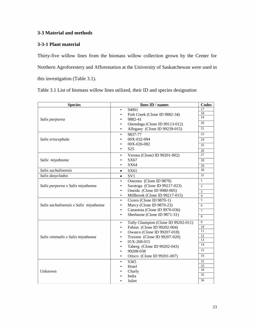
Table 3.1 List of biomass willow lines utilized, their ID and species designation

Species lines ID / names Codes

Salix purpurea

• 94001

• Fish Creek (Clone ID 9882-34)

• 9882-41

• Onondaga (Clone ID 99113-012)

• Allegany (Clone ID 99239-015)

17

18

19

20

21

Salix eriocephala

• 9837-77

• 00X-032-094

• 00X-026-082

• S25

23

24

25

26

Salix miyabeana

• Verona (Clone) ID 99201-002)

• SX67

• SX64

27

28

29

Salix sachalinensis SX61 30

Salix dasyclados SV1 31

Salix purpurea x Salix miyabeana

• Oneonta (Clone ID 9879)

• Saratoga (Clone ID 99217-023)

• Oneida (Clone ID 9980-005)

• Millbrook (Clone ID 99217-015)

1

2

3

4

Salix sachalinensis x Salix miyabeana

• Cicero (Clone ID 9870-1)

• Marcy (Clone ID 9870-23)

• Canastota (Clone ID 9970-036)

• Sherburne (Clone ID 9871-31)

5

6

7

8

Salix viminalis x Salix miyabeana

• Tully Champion (Clone ID 99202-011)

• Fabius (Clone ID 99202-004)

• Owasco (Clone ID 99207-018)

• Truxton (Clone ID 99207-020)

• 01X-268-015

• Taberg (Clone ID 99202-043)

• 99208-038

• Otisco (Clone ID 99201-007)

9

10

11

12

13

14

15

16

Unknown

• S365

• Hotel

• Charly

• India

• Juliet

32

33

34

35

36

24

The willow lines were provided as clonal material by the willow group at the

State University of New York (SUNY) and some from willow programs in Sweden. The

plantation was established on the U of S Research Farm on campus in Saskatoon in 2007

as double-row plantings (0.75 m between rows and 1.5 m between lines and 0.6 m

between trees within the row). Each row had 13 uniform plants. Leaves for DNA

extractions and flow cytometry were collected from the first plant of the first row for

each line.

Material from line SX67 could not be obtained for flow cytometry analysis. The

lines Hotel and 00X-026-082 were not considered in the ISSR analysis because of poor

DNA. Material of Salix viminalis was obtained from the Canadian Wood Fibre Centre,

Edmonton, and used in the RAPD analysis.

3-3-2 Flow cytometry

Two young leaves of each line were collected, put in between moist

paper towels and kept in separated and labelled zip-lock bags. The package was sent to

the flow cytometry laboratory at the Benaroya Research Institute,Virginia Mason,

(Washington), where the nuclear DNA content was measured using propidium stained

nuclei with a BD FACScan flow cytometer. Chicken red blood cell nuclei (2.50Pg/2C)

were used as a standard for comparison.

3-3-3 DNA extraction

Young leaves of each willow line were collected and DNA was extracted. Two

DNA extraction procedures were tested. The CTAB (cetyltrimetylammonium bromide)

25

based extraction procedure with slight modifications of the protocol developed by

Procunier et al., (1990) (Appendix1) and the ZR Plant/Seed DNA extraction kitTM

(Zymo

Research, Burlington), following the manufacturer’s procedure.

3-3-4 ISSR primers

Thirty-five ISSR primers from the University of British Columbia (UBC)

biotechnology laboratory were used (Appendix 2). Primers were 16 to 18 base pairs long

and prepared at a concentration of 5µM, and stored at -20ºC.

3-3-5 RAPD primers

Thirty-five long RAPD (15 base pairs) synthesised by Invitrogen, Canada, and 55

(10 base pairs) primers (Operon technologies, California) (Appendix 3) were tested. All

primers were diluted to a final concentration of 5µM and kept at -20ºC.

3-3-6 DNA amplification

A GeneAmp PCR System 9700 was used for DNA amlification. The PCR was

performed in a 25µl reaction containing 16.3µl water, 2.5µl buffer, 1µl of a 25mM

MgCl2, 2µl of a 5mM dNTP solution, 2µl of 5µM primer solution, 0.2µl of polymerase

and 1µl DNA template. For RAPD, the PCR was performed under the following cycling

conditions: 94ºC (3 min) for initial denaturation, followed by 35 cycles of 94ºC (45 sec)

denaturation, 37ºC (45sec) annealing and 72ºC (1min) extension. A 5min final extension

ended each PCR reaction. For ISSRs, the same protocol was used but the annealing

temperature varied among primers (Appendix 2). All reactions were set on ice prior to

26

amplification and were prepared in two steps: first, all ingredients except for the DNA

template were pipetted into a 1.5ml micro-tube, then 24µl of this mixture was pipetted

into 0.6ml micro-tube, and 1µl of DNA template added. The buffer, the MgCl2 and Taq

were used as supplied by Invitrogen, Canada.

3-3-7 Separation of amplified fragments

The amplified bands were separated by electrophoresis on a 1.25% agarose gel

(Ultrapure DNA grade agarose, BioRad) in a tris-borate- EDTA (Ethylene-Diamine-

Tetraacetic Acid) (0.5X TBE (tris base, boric acid and EDTA) buffer. The gels were pre-

stained at 0.00001% with a 0.5µg/ml ethidium bromide solution. Five micro-litres of

DNA gel loading buffer were added to the 25µl PCR reaction mixture. Gels were

photographed on a Ultraviolet (UV) transluminator with Polaroid TM

film. A 1 kb

molecular weight marker (Invitrogen, Canada) was run alongside the samples for size

assessment.

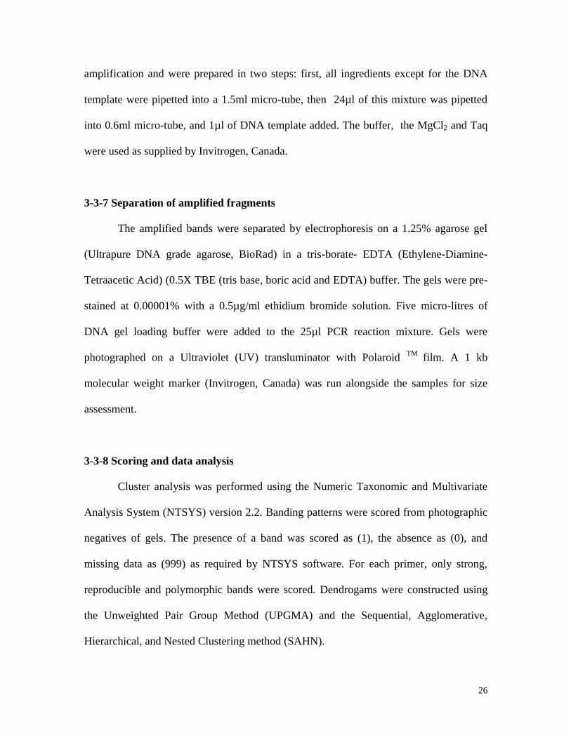
3-3-8 Scoring and data analysis

Cluster analysis was performed using the Numeric Taxonomic and Multivariate

Analysis System (NTSYS) version 2.2. Banding patterns were scored from photographic

negatives of gels. The presence of a band was scored as (1), the absence as (0), and

missing data as (999) as required by NTSYS software. For each primer, only strong,

reproducible and polymorphic bands were scored. Dendrogams were constructed using

the Unweighted Pair Group Method (UPGMA) and the Sequential, Agglomerative,

Hierarchical, and Nested Clustering method (SAHN).

27

3-4 Results

3-4-1 DNA extraction

CTAB DNA extraction from willow leaves was successful, but relatively large

amounts of foliar pigments were also extracted, which could not be removed, especially

for lines of S. eriocephala, S. dasyclados, Indiana and S365.

The ZR Plant/Seed DNA kit yielded small volumes of DNA in solution (50µl),

but the DNA was of better quality. No pigment coloration was noticed. The extraction

procedure was simple and faster (15min) and yielded 8 to 10µg of DNA from 0.15 g of

initial leaf material. DNA used in this project was extracted using the ZR Plant/Seed

DNA kit.

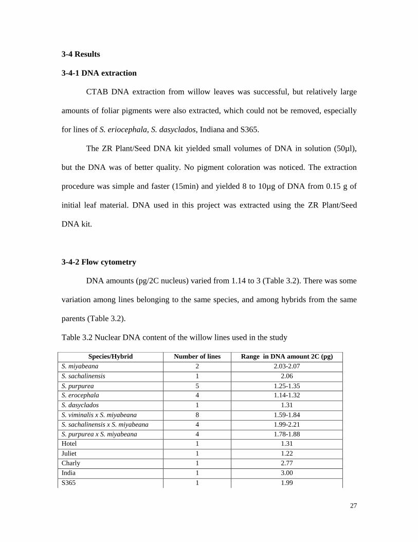
3-4-2 Flow cytometry

DNA amounts (pg/2C nucleus) varied from 1.14 to 3 (Table 3.2). There was some

variation among lines belonging to the same species, and among hybrids from the same

parents (Table 3.2).

Table 3.2 Nuclear DNA content of the willow lines used in the study

Species/Hybrid Number of lines Range in DNA amount 2C (pg)

S. miyabeana 2 2.03-2.07

S. sachalinensis 1 2.06

S. purpurea 5 1.25-1.35

S. erocephala 4 1.14-1.32

S. dasyclados 1 1.31

S. viminalis x S. miyabeana 8 1.59-1.84

S. sachalinensis x S. miyabeana 4 1.99-2.21

S. purpurea x S. miyabeana 4 1.78-1.88

Hotel 1 1.31

Juliet 1 1.22

Charly 1 2.77

India 1 3.00

S365 1 1.99

28

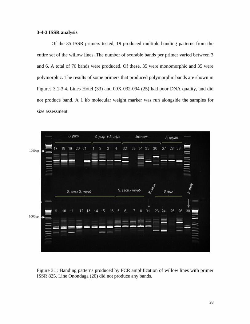
3-4-3 ISSR analysis

Of the 35 ISSR primers tested, 19 produced multiple banding patterns from the

entire set of the willow lines. The number of scorable bands per primer varied between 3

and 6. A total of 70 bands were produced. Of these, 35 were monomorphic and 35 were

polymorphic. The results of some primers that produced polymorphic bands are shown in

Figures 3.1-3.4. Lines Hotel (33) and 00X-032-094 (25) had poor DNA quality, and did

not produce band. A 1 kb molecular weight marker was run alongside the samples for

size assessment.

Figure 3.1: Banding patterns produced by PCR amplification of willow lines with primer

ISSR 825. Line Onondaga (20) did not produce any bands.

1000bp

1000bp

29

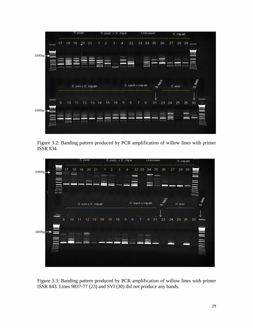
Figure 3.2: Banding pattern produced by PCR amplification of willow lines with primer

ISSR 834.

Figure 3.3: Banding pattern produced by PCR amplification of willow lines with primer

ISSR 843. Lines 9837-77 (23) and SVI (30) did not produce any bands.

1000bp

1000bp

1000bp

1000bp

30

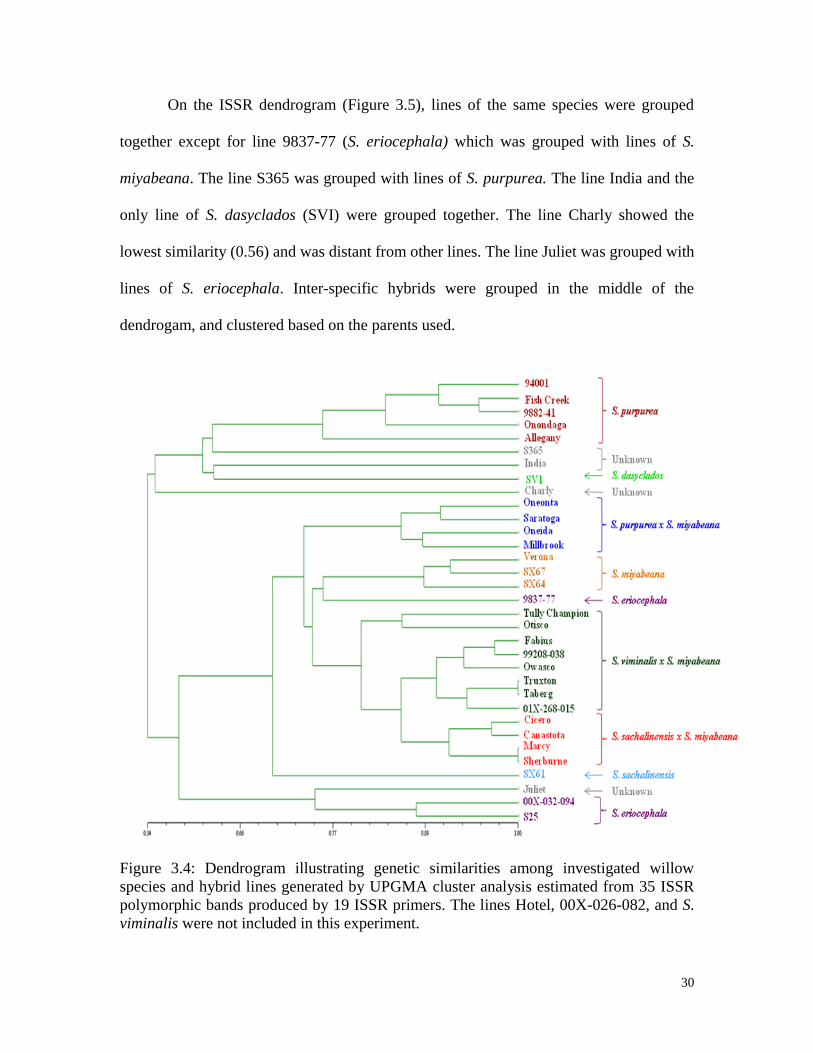
On the ISSR dendrogram (Figure 3.5), lines of the same species were grouped

together except for line 9837-77 (S. eriocephala) which was grouped with lines of S.

miyabeana. The line S365 was grouped with lines of S. purpurea. The line India and the

only line of S. dasyclados (SVI) were grouped together. The line Charly showed the

lowest similarity (0.56) and was distant from other lines. The line Juliet was grouped with

lines of S. eriocephala. Inter-specific hybrids were grouped in the middle of the

dendrogam, and clustered based on the parents used.

Figure 3.4: Dendrogram illustrating genetic similarities among investigated willow

species and hybrid lines generated by UPGMA cluster analysis estimated from 35 ISSR

polymorphic bands produced by 19 ISSR primers. The lines Hotel, 00X-026-082, and S.

viminalis were not included in this experiment.

31

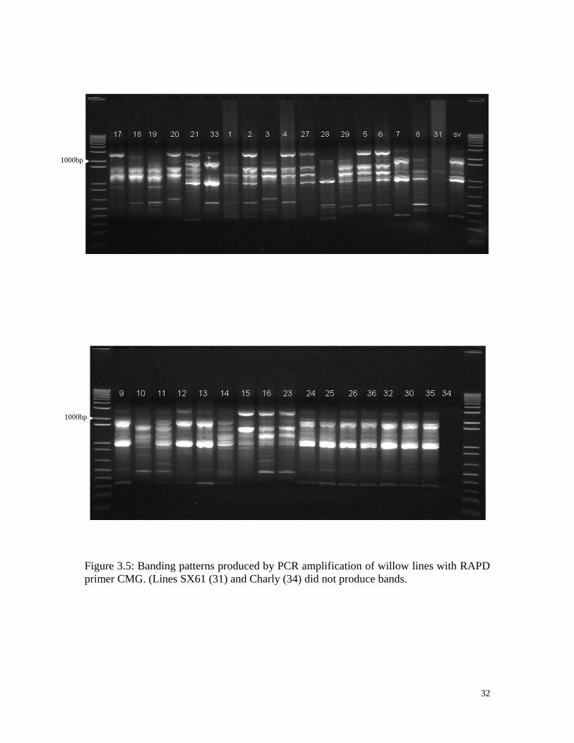
3-4-4 RAPD analysis

Each of the RAPD primers was pre-screened with a single line of each species.

Over 90 primers were tested, sixty primers were chosen to be applied to the entire set of

lines; Only Primers showing three or more bands were used to amplify the rest of the

lines. The number of scorable bands per primer varied between 3 and 10. A total of 197

scorable bands were produced. Of these, 98 were monomorphic and the remaining 99

were polymorphic and scored for cluster analysis. The lines Hotel, 00X-026-082 and S.

viminalis were included in this experiment, although not used in the ISSR analysis. An

example of RAPD banding patterns is shown (Figure 3.6).

32

Figure 3.5: Banding patterns produced by PCR amplification of willow lines with RAPD

primer CMG. (Lines SX61 (31) and Charly (34) did not produce bands.

1000bp

1000bp

33

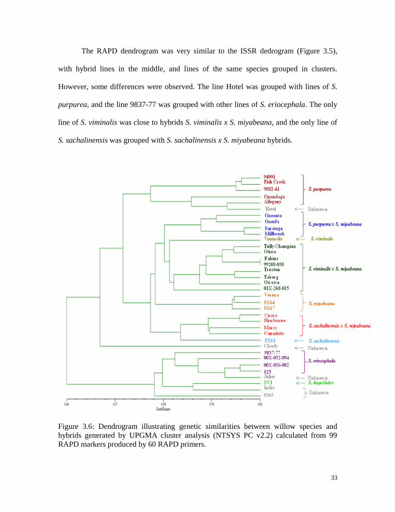
The RAPD dendrogram was very similar to the ISSR dedrogram (Figure 3.5),

with hybrid lines in the middle, and lines of the same species grouped in clusters.

However, some differences were observed. The line Hotel was grouped with lines of S.

purpurea, and the line 9837-77 was grouped with other lines of S. eriocephala. The only

line of S. viminalis was close to hybrids S. viminalis x S. miyabeana, and the only line of

S. sachalinensis was grouped with S. sachalinensis x S. miyabeana hybrids.

Figure 3.6: Dendrogram illustrating genetic similarities between willow species and

hybrids generated by UPGMA cluster analysis (NTSYS PC v2.2) calculated from 99

RAPD markers produced by 60 RAPD primers.

34

3-5 Discussion and conclusions

The objective of this series of experiments was to evaluate the nuclear DNA

content and the use of ISSR and RAPD marker techniques to assess genetic relationships

among the set of biomass willow lines being investigated by the Center for Northern

Agroforestery and Aforestation in Saskatchewan.

Flow cytometry has become widely used for the measurement of the nuclear DNA

content and ploidy screening in plants, and has proved to be rapid and more efficient than

the previous methods including Feulgen microspectrophotometry and DNA image

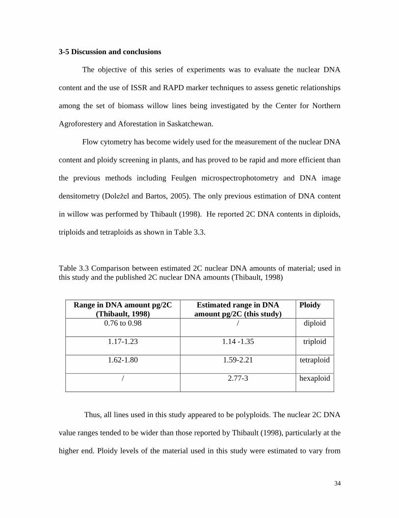
densitometry (Doležel and Bartos, 2005). The only previous estimation of DNA content

in willow was performed by Thibault (1998). He reported 2C DNA contents in diploids,

triploids and tetraploids as shown in Table 3.3.

Table 3.3 Comparison between estimated 2C nuclear DNA amounts of material; used in

this study and the published 2C nuclear DNA amounts (Thibault, 1998)

Range in DNA amount pg/2C

(Thibault, 1998)

Estimated range in DNA

amount pg/2C (this study)

Ploidy

0.76 to 0.98 / diploid

1.17-1.23 1.14 -1.35 triploid

1.62-1.80 1.59-2.21 tetraploid

/ 2.77-3 hexaploid

Thus, all lines used in this study appeared to be polyploids. The nuclear 2C DNA

value ranges tended to be wider than those reported by Thibault (1998), particularly at the

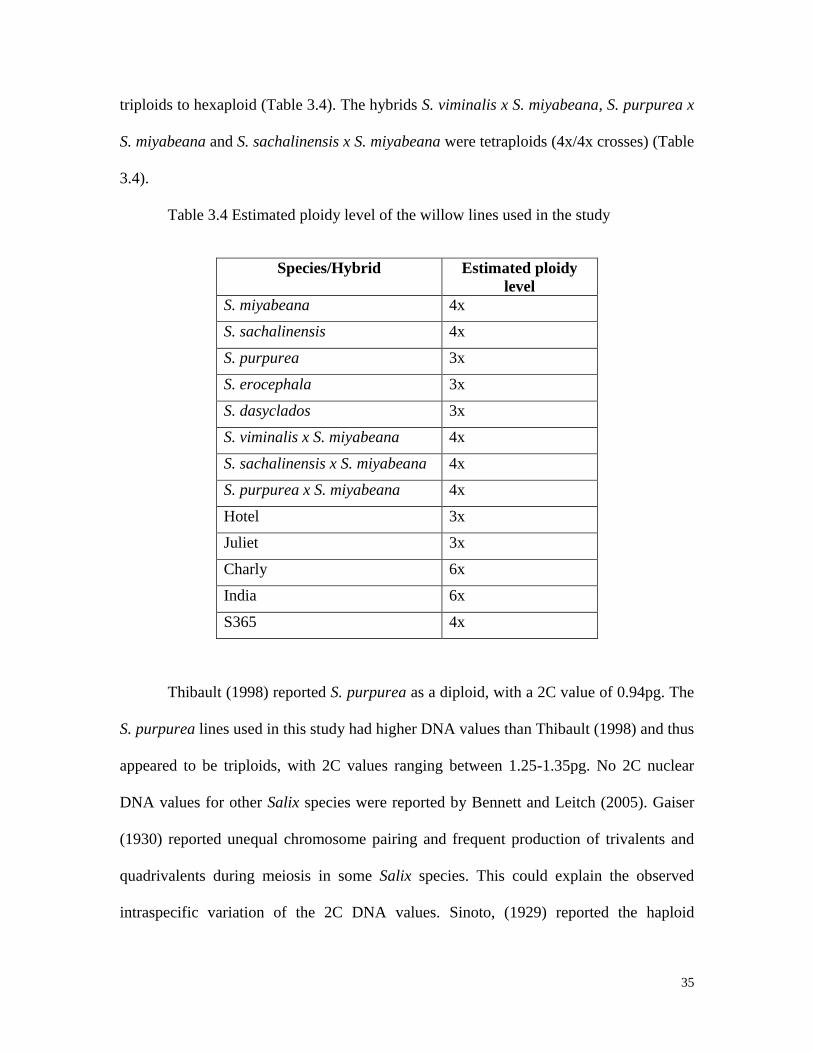
higher end. Ploidy levels of the material used in this study were estimated to vary from

35

triploids to hexaploid (Table 3.4). The hybrids S. viminalis x S. miyabeana, S. purpurea x

S. miyabeana and S. sachalinensis x S. miyabeana were tetraploids (4x/4x crosses) (Table

3.4).

Table 3.4 Estimated ploidy level of the willow lines used in the study

Thibault (1998) reported S. purpurea as a diploid, with a 2C value of 0.94pg. The

S. purpurea lines used in this study had higher DNA values than Thibault (1998) and thus

appeared to be triploids, with 2C values ranging between 1.25-1.35pg. No 2C nuclear

DNA values for other Salix species were reported by Bennett and Leitch (2005). Gaiser

(1930) reported unequal chromosome pairing and frequent production of trivalents and

quadrivalents during meiosis in some Salix species. This could explain the observed

intraspecific variation of the 2C DNA values. Sinoto, (1929) reported the haploid

Species/Hybrid Estimated ploidy

level

S. miyabeana 4x

S. sachalinensis 4x

S. purpurea 3x

S. erocephala 3x

S. dasyclados 3x

S. viminalis x S. miyabeana 4x

S. sachalinensis x S. miyabeana 4x

S. purpurea x S. miyabeana 4x

Hotel 3x

Juliet 3x

Charly 6x

India 6x

S365 4x

36

chromosome number of S. sachalinensis to be n=19, but mentioned the existence of n=24

haploid cells in a form of S. sachalinensis from Hokkaido. No information on

chromosome number of S. miyabeana, and S. eriocephala was found in the literature.

Intra-specific variation in genome size has been reported in many plant species (Bennett,

1985). The results of this experiment confirmed the variability of 2C nuclear DNA values

and ploidy levels both within and between Salix species (Hakansson, 1955; Suda and

Argus, 1968; Thibault, 1998). All hybrid lines were tetraploids from crosses between

tetraploid parents.

Both RAPD and ISSR dendrograms showed the same clusters with some minor

differences. The ISSR dendrogram grouped line 9377-77 with lines of S. miyabeana,

whereas the RAPD dendrogram, grouped the same line along with other lines of S.

eriocephala. This difference could be due to scoring errors or to the reduced number of

scoring data (35) used to construct the ISSR dendrogram. The RAPD dendrogram

produced a slightly better separation of clusters with a higher number of scoring data

(99).

The line Hotel was clustered with other lines of S. purpurea, line Juliet was

clustered with lines of S. eriocephala, and lines S365 and India were in both RAPD and

ISSR studies grouped with the only line of S. dasyclados (SVI).

ISSR primers produced fewer bands (3 to 6), which appeared stronger and

reproducible. RAPD primers produced more bands (5-9), but most of them appeared

weak and less reproducible compared to ISSRs.

37

3-5-1 Markers for specific lines

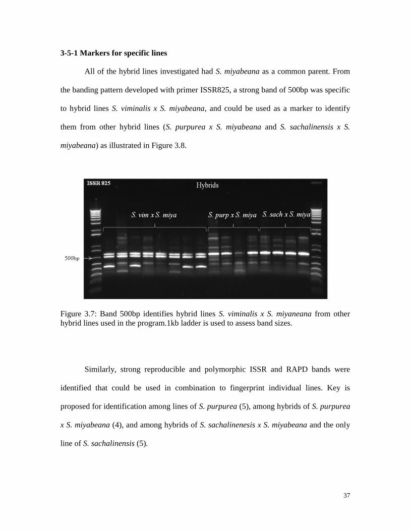
All of the hybrid lines investigated had S. miyabeana as a common parent. From

the banding pattern developed with primer ISSR825, a strong band of 500bp was specific

to hybrid lines S. viminalis x S. miyabeana, and could be used as a marker to identify

them from other hybrid lines (S. purpurea x S. miyabeana and S. sachalinensis x S.

miyabeana) as illustrated in Figure 3.8.

Figure 3.7: Band 500bp identifies hybrid lines S. viminalis x S. miyaneana from other

hybrid lines used in the program.1kb ladder is used to assess band sizes.

Similarly, strong reproducible and polymorphic ISSR and RAPD bands were

identified that could be used in combination to fingerprint individual lines. Key is

proposed for identification among lines of S. purpurea (5), among hybrids of S. purpurea

x S. miyabeana (4), and among hybrids of S. sachalinenesis x S. miyabeana and the only

line of S. sachalinensis (5).

38

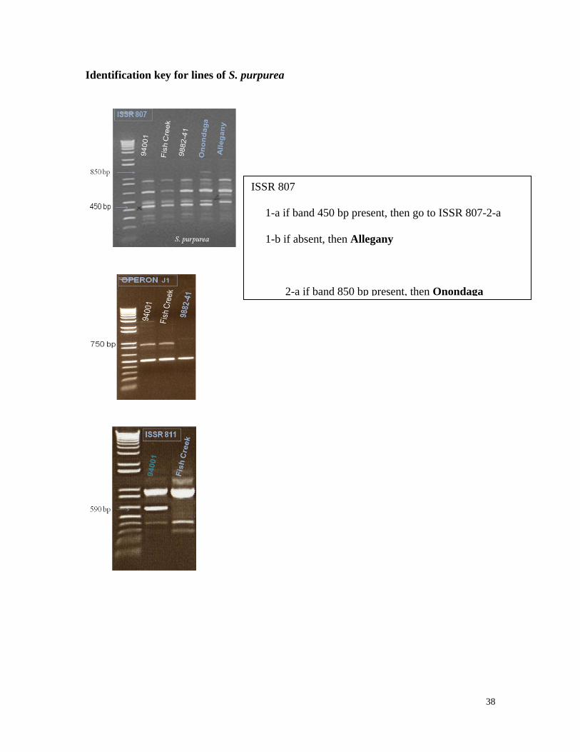
Identification key for lines of S. purpurea

ISSR 807

1-a if band 450 bp present, then go to ISSR 807-2-a

1-b if absent, then Allegany

2-a if band 850 bp present, then Onondaga

2-b if absent, then go to operon J1

Operon J1

1-a if band 750 present, then go to ISSR 811

1-b if absent, then 9882-41

ISSR 811

1-a if band 590 present, then 94001

1-b if absent, then Fish Creek

39

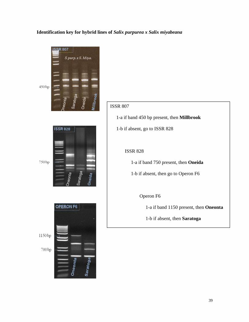
Identification key for hybrid lines of Salix purpurea x Salix miyabeana

ISSR 807

1-a if band 450 bp present, then Millbrook

1-b if absent, go to ISSR 828

ISSR 828

1-a if band 750 present, then Oneida

1-b if absent, then go to Operon F6

Operon F6

1-a if band 1150 present, then Oneonta

1-b if absent, then Saratoga

40

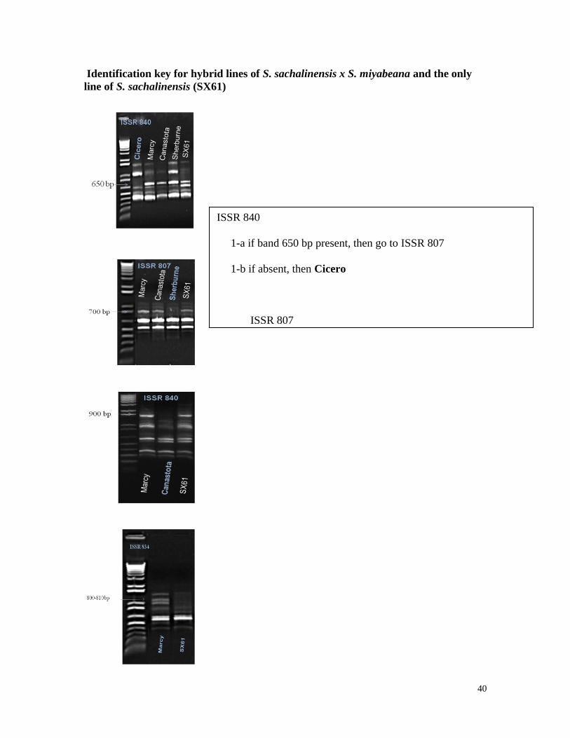
Identification key for hybrid lines of S. sachalinensis x S. miyabeana and the only

line of S. sachalinensis (SX61)

ISSR 840

1-a if band 650 bp present, then go to ISSR 807

1-b if absent, then Cicero

ISSR 807

1-a if band 700 bp present, then go to ISSR 840

1-b if absent, then Sherburne

ISSR 840

1-a if band 900 bp present, then go to ISSR 829

1-b if absent, then Canastota

ISSR 834

1-a if band 800/810 bp present, then Marcy

1-b if absent, then SX61

41

4-THE USE OF 18S-5.8S-28S INTERNAL TRANSCRIBED SPACER (ITS) FOR

SPECIES IDENTIFICATION IN THE GENUS Salix

4-1 Abstract

Given that morphological identification of willow species used in the project is

difficult, the DNA region coding for ribosomal RNA including the entire 5.8S RNA

region and the internal transcribed spacers (ITS1 and ITS2) was amplified and sequenced

to assess sequence homology between five Salix species (Salix purpurea, Salix

eriocephala, Salix sachalinensis, and Salix dasyclados). The total length of the amplified

region was 601bp, with the ITS1, 5.8 S and ITS2 being 223, 163, and 215bp respectively.

Intra- and inter-species SNPs were observed, 6 within ITS1, and 3 within ITS2. No

polymorphisms were found in the 5.8S gene. The low rate of variation within the

sequenced ITS fragment between species supports the monophyly of the five species

involved in this study, and confirms their belonging to the subgenus Caprisalix. SCAR

primers were designed from species specific polymorphic nucleotides and applied to the

willow collection to test their use for species identification. A species identification key

based on SNPs is proposed.

42

4-2 Introduction

Nuclear rRNA genes provide markers for phylogeny at a variety of taxonomic

levels (Soltis and Kuzoff, 1993). The 18S-5.8S-28S tandem repeats are located in the

nucleolar organizing region of satellited chromosomes. Each repeat unit consists of a

single transcribed region for the 18S, 5.8S and 28S ribosomal RNAs, two small internal

transcribed spacers (ITS1 and ITS2) and a large external non transcribed inter-genic

spacer (IGS) (Flavell, 1986). ITS sequences are easy to amplify, even with small

quantities of DNA, and show a high level of variation even between closely related

species (Chen et al., 2001; Baldwin, 1992). DNA coding for the 18S, 5.8S, and 28S

rRNAs are highly conserved. The spacers undergo concerted evolution where they evolve

relatively together by accumulating mutations, and provide a source of polymorphisms

between species and genera (Downie and Downie, 1996).

In this experiment, the internal transcribed spacers (ITS1 and ITS2) were investigated for

length and DNA sequence variation among the willow species (Salix purpurea, Salix

miyabeana, Salix eriocephala, Salix dasyclados, Salix sachalinensis) used in this project.

SCAR markers were developed from species-specific polymorphisms.

43

4-3 Materials and methods

4-3-1 Plant material

Five willow lines were randomly chosen from among the biomass willow

collection grown by the Center for Northern Agroforrestery and Afforestation of the

University of Saskatchewan for this experiment (Table 4.1), each representing one

species used in the project.

Table 4.1 Selected willow lines for ITS analysis

Species S. purpurea S. eriocephala S. miyabeana S. sachalinensis S. dasyclados

Clone ID 94001 9837-77 SX64 SX61 SVI

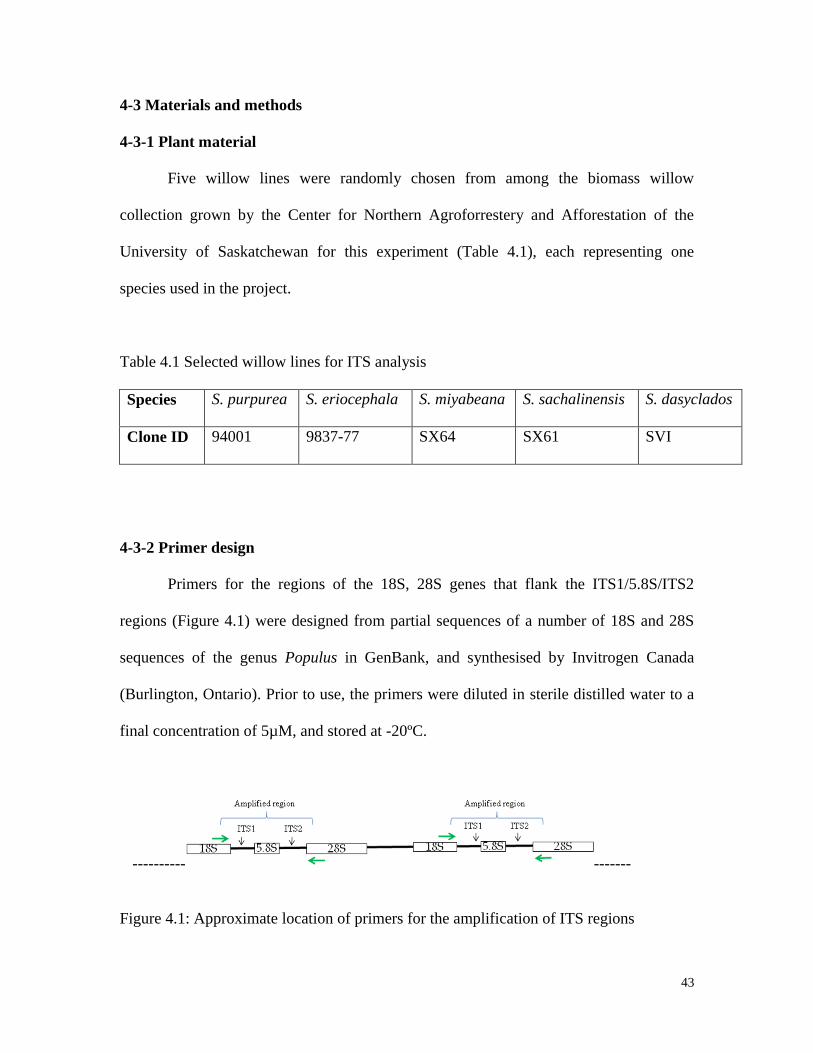
4-3-2 Primer design

Primers for the regions of the 18S, 28S genes that flank the ITS1/5.8S/ITS2

regions (Figure 4.1) were designed from partial sequences of a number of 18S and 28S

sequences of the genus Populus in GenBank, and synthesised by Invitrogen Canada

(Burlington, Ontario). Prior to use, the primers were diluted in sterile distilled water to a

final concentration of 5µM, and stored at -20ºC.

---------- -------

Figure 4.1: Approximate location of primers for the amplification of ITS regions

44

4-3-3 DNA extraction

Young leaves of the selected lines were collected. One hundred and fifty

milligram of leaf material was used for DNA extraction, following the ZR Plant/Seed

DNA extraction kitTM

(Zymo Research, Burlington).

4-3-4 DNA amplification and gel electrophoresis

DNA amplification was performed using a GeneAmp PCR System 9700. Each

PCR was performed in a 25µl reaction containing 16.3µl of water, 2.5µl buffer, 1µl

MgCl2, 1µl of the 5µM 18S primer solution, 1µl of the 5µM 28S primer solution, 2µl of a

5mM dNTP solution, 0.2 µl of Taq polymerase (Invitrogen Canada) and 1µl of the DNA

template. The buffer, the MgCl2 and Taq were used as supplied by Invitrogen, Canada.

The thermo-cycler was set for the following cycling conditions: 94º C (3min) for initial

denaturation, followed by 35 cycles of 94ºC (45sec) denaturation, 65º C (45sec)

annealing and 72º C (1min) extension. Each PCR reaction ended with a 5min final

extension period. The amplification reaction was repeated to check for reproducibility.

From the 25µl of each PCR reaction, 19µl were used for electrophoresis and 6µl were

retained for cloning and sequencing.

Amplified fragments were separated by gel electrophoresis on a 1% agarose gel in

tris borate EDTA (0.5X TBE) buffer, and visualised by pre-staining with ethidium

bromide (0.1µg /ml). Five micro-litres of DNA gel loading buffer were added to each

reaction before loading the gel. A 1kb molecular weight marker was run along the side of

the samples for size assessment. Stained ITS fragments were viewed under UV light.

45

4-3-5 Cloning and sequencing

Two micro-litres of the ITS fragment PCR reaction were used for cloning. The

ITS fragments were ligated into pCR®4-TOPO® vector plasmid (Invitrogen, Canada).

The recombinant plasmid vectors were transformed into One Shot ® TOPO10 competent

E.coli cells and grown overnight on LB plates containing 100µl/ml of a 50 mg/ml

ampicillin solution. Ten isolated colonies were aseptically picked and grown separately

on 5ml LB broth (Gibco) medium containing 5µl of a 50mg/ml ampicillin solution.

To confirm the presence of the appropriate insert, PCR reactions were carried out

using 1µl of each colony as template. The GeneAmp PCR System 9700 was used. Each

PCR was performed in a 25µl reaction containing 16.3µl of water, 2.5µl buffer, 1µl

MgCl2, 1µl each of the primers used to initially create the fragment, 2µl of dNTP, 0.2µl

of Taq polymerase (Invitrogen, Canada), and 1µl of the bacterial culture. The

amplification program used for PCR was the same as that initially used to produce the

fragments of interest.

All reactions were analysed on a 1% agarose gel in tris borate EDTA (0.5X TBE)

buffer, and visualised by pre-staining with ethidium bromide (0.1µg /ml). Five micro-

litres of DNA gel loading buffer were added to each reaction before loading the gel. A

1kb molecular weight marker was run along side of the samples for size assessment, and

the bands were viewed under UV light.

Colonies with the expected insert size were purified following the QIAprep ®

Miniprep kit. Extracted recombinant vectors were sent for sequencing at the Plant

Biotechnology Institute (PBI) in Saskatoon (Canada). The whole experiment was

46

repeated once for each line to produce up to 20 sequences per line. DNAMAN software

(Lynnon Biosoff, 1994-1997) was used for sequence alignment.

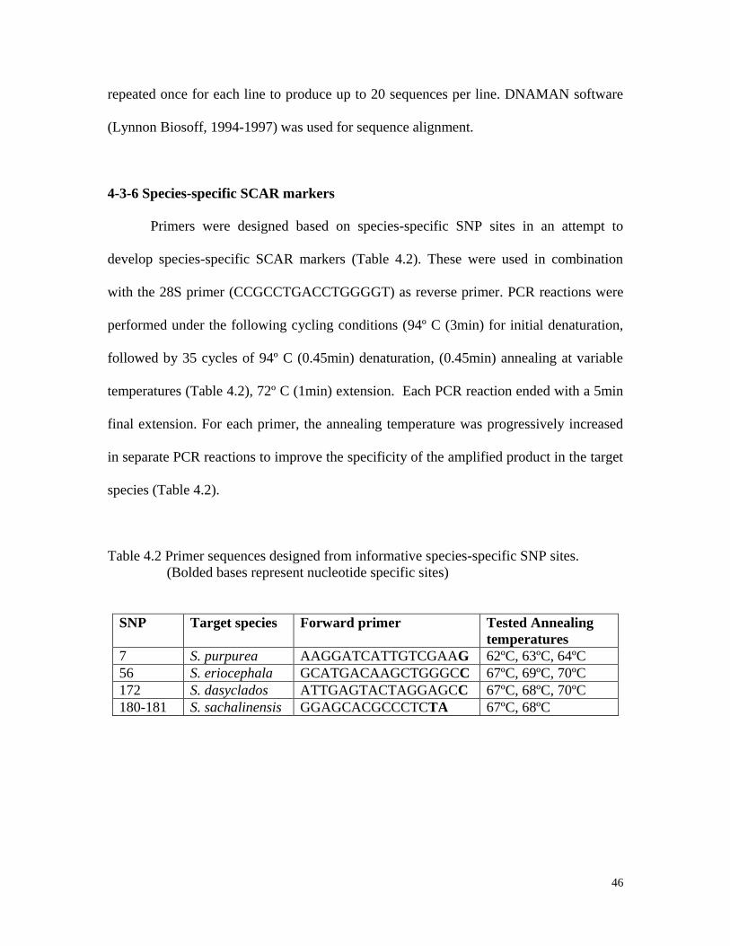
4-3-6 Species-specific SCAR markers

Primers were designed based on species-specific SNP sites in an attempt to

develop species-specific SCAR markers (Table 4.2). These were used in combination

with the 28S primer (CCGCCTGACCTGGGGT) as reverse primer. PCR reactions were

performed under the following cycling conditions (94º C (3min) for initial denaturation,

followed by 35 cycles of 94º C (0.45min) denaturation, (0.45min) annealing at variable

temperatures (Table 4.2), 72º C (1min) extension. Each PCR reaction ended with a 5min

final extension. For each primer, the annealing temperature was progressively increased

in separate PCR reactions to improve the specificity of the amplified product in the target

species (Table 4.2).

Table 4.2 Primer sequences designed from informative species-specific SNP sites.

(Bolded bases represent nucleotide specific sites)

SNP Target species Forward primer Tested Annealing

temperatures

7 S. purpurea AAGGATCATTGTCGAAG 62ºC, 63ºC, 64ºC

56 S. eriocephala GCATGACAAGCTGGGCC 67ºC, 69ºC, 70ºC

172 S. dasyclados ATTGAGTACTAGGAGCC 67ºC, 68ºC, 70ºC

180-181 S. sachalinensis GGAGCACGCCCTCTA 67ºC, 68ºC

47

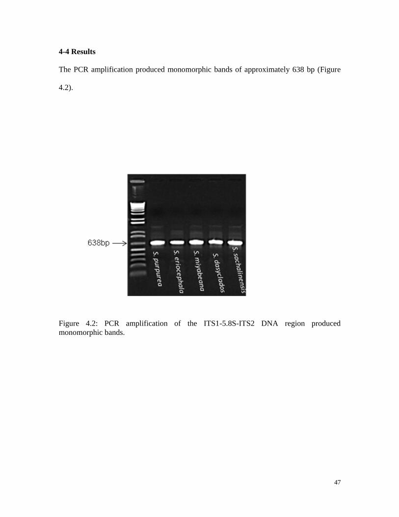
4-4 Results

The PCR amplification produced monomorphic bands of approximately 638 bp (Figure

4.2).

Figure 4.2: PCR amplification of the ITS1-5.8S-ITS2 DNA region produced

monomorphic bands.

48

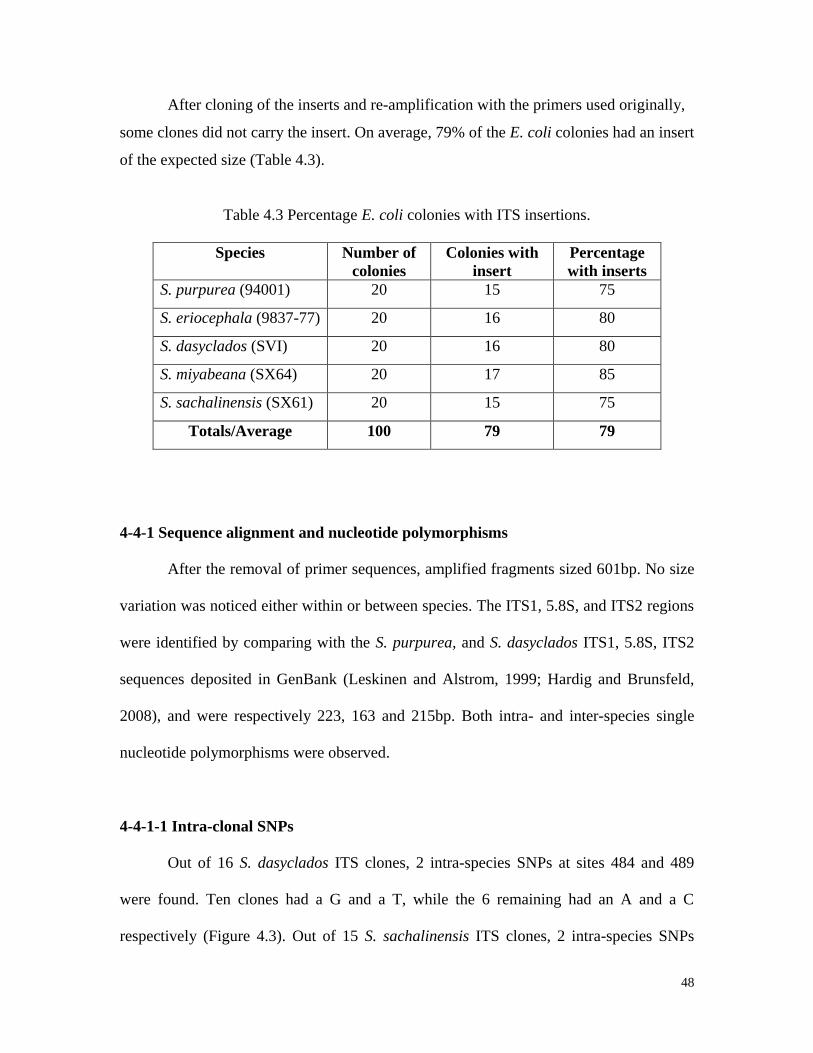
After cloning of the inserts and re-amplification with the primers used originally,

some clones did not carry the insert. On average, 79% of the E. coli colonies had an insert

of the expected size (Table 4.3).

Table 4.3 Percentage E. coli colonies with ITS insertions.

Species Number of

colonies

Colonies with

insert

Percentage

with inserts

S. purpurea (94001) 20 15 75

S. eriocephala (9837-77) 20 16 80

S. dasyclados (SVI) 20 16 80

S. miyabeana (SX64) 20 17 85

S. sachalinensis (SX61) 20 15 75

Totals/Average 100 79 79

4-4-1 Sequence alignment and nucleotide polymorphisms

After the removal of primer sequences, amplified fragments sized 601bp. No size

variation was noticed either within or between species. The ITS1, 5.8S, and ITS2 regions

were identified by comparing with the S. purpurea, and S. dasyclados ITS1, 5.8S, ITS2

sequences deposited in GenBank (Leskinen and Alstrom, 1999; Hardig and Brunsfeld,

2008), and were respectively 223, 163 and 215bp. Both intra- and inter-species single

nucleotide polymorphisms were observed.

4-4-1-1 Intra-clonal SNPs

Out of 16 S. dasyclados ITS clones, 2 intra-species SNPs at sites 484 and 489

were found. Ten clones had a G and a T, while the 6 remaining had an A and a C

respectively (Figure 4.3). Out of 15 S. sachalinensis ITS clones, 2 intra-species SNPs

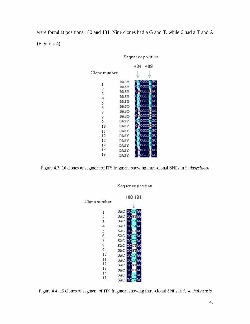
49

were found at positions 180 and 181. Nine clones had a G and T, while 6 had a T and A

(Figure 4.4).

Figure 4.3: 16 clones of segment of ITS fragment showing intra-clonal SNPs in S. dasyclados

Figure 4.4: 15 clones of segment of ITS fragment showing intra-clonal SNPs in S. sachalinensis

50

These intra-species SNPs led to the identification of two consensuses ITS

sequences for S. dasyclados (S. dasy1 and S. dasy2) and two for S. sachalinensis (S.

sacha1 and S. sacha2) (Figures 4.5- 4.7). No intra-species SNP were recorded among ITS

clones of S. purpurea, S. miyabeana and S. eriocephala and one consensus ITS sequence

was consequently identified for each of those species (Figures 4.5-4.7).

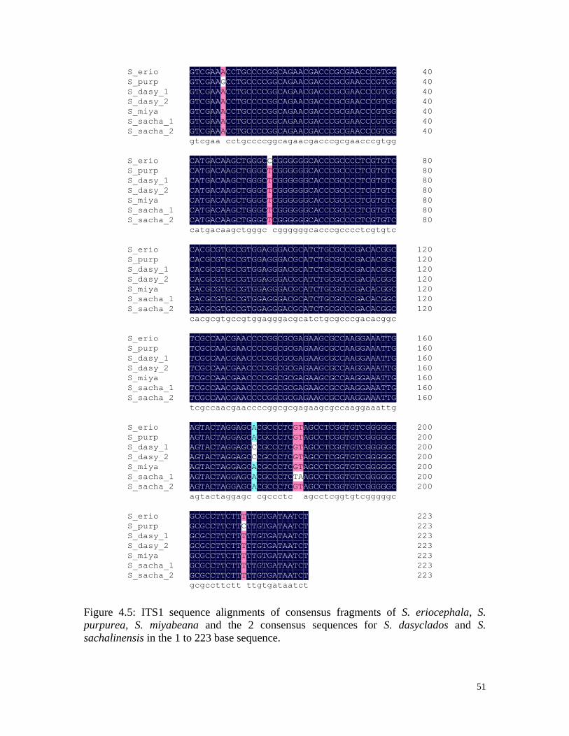
51

40S_erio

40S_purp

40S_dasy_1

40S_dasy_2

40S_miya

40S_sacha_1

40S_sacha_2

GTCGAAACCTGCCCCGGCAGAACGACCCGCGAACCCGTGG

GTCGAAGCCTGCCCCGGCAGAACGACCCGCGAACCCGTGG

GTCGAAACCTGCCCCGGCAGAACGACCCGCGAACCCGTGG

GTCGAAACCTGCCCCGGCAGAACGACCCGCGAACCCGTGG

GTCGAAACCTGCCCCGGCAGAACGACCCGCGAACCCGTGG

GTCGAAACCTGCCCCGGCAGAACGACCCGCGAACCCGTGG

GTCGAAACCTGCCCCGGCAGAACGACCCGCGAACCCGTGG

g

G

G

G

G

G

G

G

t

T

T

T

T

T

T

T

c

C

C

C

C

C

C

C

g

G

G

G

G

G

G

G

a

A

A

A

A

A

A

A

a

A

A

A

A

A

A

A

A

A

A

A

A

A

c

C

C

C

C

C

C

C

c

C

C

C

C

C

C

C

t

T

T

T

T

T

T

T

g

G

G

G

G

G

G

G

c

C

C

C

C

C

C

C

c

C

C

C

C

C

C

C

c

C

C

C

C

C

C

C

c

C

C

C

C

C

C

C

g

G

G

G

G

G

G

G

g

G

G

G

G

G

G

G

c

C

C

C

C

C

C

C

a

A

A

A

A

A

A

A

g

G

G

G

G

G

G

G

a

A

A

A

A

A

A

A

a

A

A

A

A

A

A

A

c

C

C

C

C

C

C

C

g

G

G

G

G

G

G

G

a

A

A

A

A

A

A

A

c

C

C

C

C

C

C

C

c

C

C

C

C

C

C

C

c

C

C

C

C

C

C

C

g

G

G

G

G

G

G

G

c

C

C

C

C

C

C

C

g

G

G

G

G

G

G

G

a

A

A

A

A

A

A

A

a

A

A

A

A

A

A

A

c

C

C

C

C

C

C

C

c

C

C

C

C

C

C

C

c

C

C

C

C

C

C

C

g

G

G

G

G

G

G

G

t

T

T

T

T

T

T

T

g

G

G

G

G

G

G

G

g

G

G

G

G

G

G

G

80S_erio

80S_purp

80S_dasy_1

80S_dasy_2

80S_miya

80S_sacha_1

80S_sacha_2

CATGACAAGCTGGGCCCGGGGGGCACCCGCCCCTCGTGTC

CATGACAAGCTGGGCTCGGGGGGCACCCGCCCCTCGTGTC

CATGACAAGCTGGGCTCGGGGGGCACCCGCCCCTCGTGTC

CATGACAAGCTGGGCTCGGGGGGCACCCGCCCCTCGTGTC

CATGACAAGCTGGGCTCGGGGGGCACCCGCCCCTCGTGTC

CATGACAAGCTGGGCTCGGGGGGCACCCGCCCCTCGTGTC

CATGACAAGCTGGGCTCGGGGGGCACCCGCCCCTCGTGTC

c

C

C

C

C

C

C

C

a

A

A

A

A

A

A

A

t

T

T

T

T

T

T

T

g

G

G

G

G

G

G

G

a

A

A

A

A

A

A

A

c

C

C

C

C

C

C

C

a

A

A

A

A

A

A

A

a

A

A

A

A

A

A

A

g

G

G

G

G

G

G

G

c

C

C

C

C

C

C

C

t

T

T

T

T

T

T

T

g

G

G

G

G

G

G

G

g

G

G

G

G

G

G

G

g

G

G

G

G

G

G

G

c

C

C

C

C

C

C

C

T

T

T

T

T

T

c

C

C

C

C

C

C

C

g

G

G

G

G

G

G

G

g

G

G

G

G

G

G

G

g

G

G

G

G

G

G

G

g

G

G

G

G

G

G

G

g

G

G

G

G

G

G

G

g

G

G

G

G

G

G

G

c

C

C

C

C

C

C

C

a

A

A

A

A

A

A

A

c

C

C

C

C

C

C

C

c

C

C

C

C

C

C

C

c

C

C

C

C

C

C

C

g

G

G

G

G

G

G

G

c

C

C

C

C

C

C

C

c

C

C

C

C

C

C

C

c

C

C

C

C

C

C

C

c

C

C

C

C

C

C

C

t

T

T

T

T

T

T

T

c

C

C

C

C

C

C

C

g

G

G

G

G

G

G

G

t

T

T

T

T

T

T

T

g

G

G

G

G

G

G

G

t

T

T

T

T

T

T

T

c

C

C

C

C

C

C

C

120S_erio

120S_purp

120S_dasy_1

120S_dasy_2

120S_miya

120S_sacha_1

120S_sacha_2

CACGCGTGCCGTGGAGGGACGCATCTGCGCCCGACACGGC

CACGCGTGCCGTGGAGGGACGCATCTGCGCCCGACACGGC

CACGCGTGCCGTGGAGGGACGCATCTGCGCCCGACACGGC

CACGCGTGCCGTGGAGGGACGCATCTGCGCCCGACACGGC

CACGCGTGCCGTGGAGGGACGCATCTGCGCCCGACACGGC

CACGCGTGCCGTGGAGGGACGCATCTGCGCCCGACACGGC

CACGCGTGCCGTGGAGGGACGCATCTGCGCCCGACACGGC

c

C

C

C

C

C

C

C

a

A

A

A

A

A

A

A

c

C

C

C

C

C

C

C

g

G

G

G

G

G

G

G

c

C

C

C

C

C

C

C

g

G

G

G

G

G

G

G

t

T

T

T

T

T

T

T

g

G

G

G

G

G

G

G

c

C

C

C

C

C

C

C

c

C

C

C

C

C

C

C

g

G

G

G

G

G

G

G

t

T

T

T

T

T

T

T

g

G

G

G

G

G

G

G

g

G

G

G

G

G

G

G

a

A

A

A

A

A

A

A

g

G

G

G

G

G

G

G

g

G

G

G

G

G

G

G

g

G

G

G

G

G

G

G

a

A

A

A

A

A

A

A

c

C

C

C

C

C

C

C

g

G

G

G

G

G

G

G

c

C

C

C

C

C

C

C

a

A

A

A

A

A

A

A

t

T

T

T

T

T

T

T

c

C

C

C

C

C

C

C

t

T

T

T

T

T

T

T

g

G

G

G

G

G

G

G

c

C

C

C

C

C

C

C

g

G

G

G

G

G

G

G

c

C

C

C

C

C

C

C

c

C

C

C

C

C

C

C

c

C

C

C

C

C

C

C

g

G

G

G

G

G

G

G

a

A

A

A

A

A

A

A

c

C

C

C

C

C

C

C

a

A

A

A

A

A

A

A

c

C

C

C

C

C

C

C

g

G

G

G

G

G

G

G

g

G

G

G

G

G

G

G

c

C

C

C

C

C

C

C

160S_erio

160S_purp

160S_dasy_1

160S_dasy_2

160S_miya

160S_sacha_1

160S_sacha_2

TCGCCAACGAACCCCGGCGCGAGAAGCGCCAAGGAAATTG

TCGCCAACGAACCCCGGCGCGAGAAGCGCCAAGGAAATTG

TCGCCAACGAACCCCGGCGCGAGAAGCGCCAAGGAAATTG

TCGCCAACGAACCCCGGCGCGAGAAGCGCCAAGGAAATTG

TCGCCAACGAACCCCGGCGCGAGAAGCGCCAAGGAAATTG

TCGCCAACGAACCCCGGCGCGAGAAGCGCCAAGGAAATTG

TCGCCAACGAACCCCGGCGCGAGAAGCGCCAAGGAAATTG

t

T

T

T

T

T

T

T

c

C

C

C

C

C

C

C

g

G

G

G

G

G

G

G

c

C

C

C

C

C

C

C

c

C

C

C

C

C

C

C

a

A

A

A

A

A

A

A

a

A

A

A

A

A

A

A

c

C

C

C

C

C

C

C

g

G

G

G

G

G

G

G

a

A

A

A

A

A

A

A

a

A

A

A

A

A

A

A

c

C

C

C

C

C

C

C

c

C

C

C

C

C

C

C

c

C

C

C

C

C

C

C

c

C

C

C

C

C

C

C

g

G

G

G

G

G

G

G

g

G

G

G

G

G

G

G

c

C

C

C

C

C

C

C

g

G

G

G

G

G

G

G

c

C

C

C

C

C

C

C

g

G

G

G

G

G

G

G

a

A

A

A

A

A

A

A

g

G

G

G

G

G

G

G

a

A

A

A

A

A

A

A

a

A

A

A

A

A

A

A

g

G

G

G

G

G

G

G

c

C

C

C

C

C

C

C

g

G

G

G

G

G

G

G

c

C

C

C

C

C

C

C

c

C

C

C

C

C

C

C

a

A

A

A

A

A

A

A

a

A

A

A

A

A

A

A

g

G

G

G

G

G

G

G

g

G

G

G

G

G

G

G

a

A

A

A

A

A

A

A

a

A

A

A

A

A

A

A

a

A

A

A

A

A

A

A

t

T

T

T

T

T

T

T

t

T

T

T

T

T

T

T

g

G

G

G

G

G

G

G

200S_erio

200S_purp

200S_dasy_1

200S_dasy_2

200S_miya

200S_sacha_1

200S_sacha_2

AGTACTAGGAGCACGCCCTCGTAGCCTCGGTGTCGGGGGC

AGTACTAGGAGCACGCCCTCGTAGCCTCGGTGTCGGGGGC

AGTACTAGGAGCCCGCCCTCGTAGCCTCGGTGTCGGGGGC

AGTACTAGGAGCCCGCCCTCGTAGCCTCGGTGTCGGGGGC

AGTACTAGGAGCACGCCCTCGTAGCCTCGGTGTCGGGGGC

AGTACTAGGAGCACGCCCTCTAAGCCTCGGTGTCGGGGGC

AGTACTAGGAGCACGCCCTCGTAGCCTCGGTGTCGGGGGC

a

A

A

A

A

A

A

A

g

G

G

G

G

G

G

G

t

T

T

T

T

T

T

T

a

A

A

A

A

A

A

A

c

C

C

C

C

C

C

C

t

T

T

T

T

T

T

T

a

A

A

A

A

A

A

A

g

G

G

G

G

G

G

G

g

G

G

G

G

G

G

G

a

A

A

A

A

A

A

A

g

G

G

G

G

G

G

G

c

C

C

C

C

C

C

C

A

A

A

A

A

c

C

C

C

C

C

C

C

g

G

G

G

G

G

G

G

c

C

C

C

C

C

C

C

c

C

C

C

C

C

C

C

c

C

C

C

C

C

C

C

t

T

T

T

T

T

T

T

c

C

C

C

C

C

C

C

G

G

G

G

G

G

T

T

T

T

T

T

a

A

A

A

A

A

A

A

g

G

G

G

G

G

G

G

c

C

C

C

C

C

C

C

c

C

C

C

C

C

C

C

t

T

T

T

T

T

T

T

c

C

C

C

C

C

C

C

g

G

G

G

G

G

G

G

g

G

G

G

G

G

G

G

t

T

T

T

T

T

T

T

g

G

G

G

G

G

G

G

t

T

T

T

T

T

T

T

c

C

C

C

C

C

C

C

g

G

G

G

G

G

G

G

g

G

G

G

G

G

G

G

g

G

G

G

G

G

G

G

g

G

G

G

G

G

G

G

g

G

G

G

G

G

G

G

c

C

C

C

C

C

C

C

223S_erio

223S_purp

223S_dasy_1

223S_dasy_2

223S_miya

223S_sacha_1

223S_sacha_2

GCGCCTTCTTTTTGTGATAATCT

GCGCCTTCTTCTTGTGATAATCT

GCGCCTTCTTTTTGTGATAATCT

GCGCCTTCTTTTTGTGATAATCT

GCGCCTTCTTTTTGTGATAATCT

GCGCCTTCTTTTTGTGATAATCT

GCGCCTTCTTTTTGTGATAATCT

g

G

G

G

G

G

G

G

c

C

C

C

C

C

C

C

g

G

G

G

G

G

G

G

c

C

C

C

C

C

C

C

c

C

C

C

C

C

C

C

t

T

T

T

T

T

T

T

t

T

T

T

T

T

T

T

c

C

C

C

C

C

C

C

t

T

T

T

T

T

T

T

t

T

T

T

T

T

T

T

T

T

T

T

T

T

t

T

T

T

T

T

T

T

t

T

T

T

T

T

T

T

g

G

G

G

G

G

G

G

t

T

T

T

T

T

T

T

g

G

G

G

G

G

G

G

a

A

A

A

A

A

A

A

t

T

T

T

T

T

T

T

a

A

A

A

A

A

A

A

a

A

A

A

A

A

A

A

t

T

T

T

T

T

T

T

c

C

C

C

C

C

C

C

t

T

T

T

T

T

T

T

Figure 4.5: ITS1 sequence alignments of consensus fragments of S. eriocephala, S.

purpurea, S. miyabeana and the 2 consensus sequences for S. dasyclados and S.

sachalinensis in the 1 to 223 base sequence.

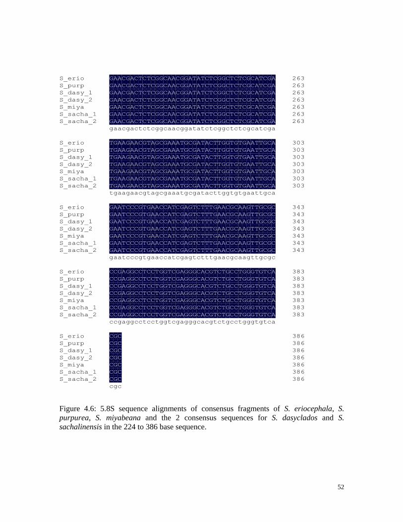
52

263S_erio

263S_purp

263S_dasy_1

263S_dasy_2

263S_miya

263S_sacha_1

263S_sacha_2

GAACGACTCTCGGCAACGGATATCTCGGCTCTCGCATCGA

GAACGACTCTCGGCAACGGATATCTCGGCTCTCGCATCGA

GAACGACTCTCGGCAACGGATATCTCGGCTCTCGCATCGA

GAACGACTCTCGGCAACGGATATCTCGGCTCTCGCATCGA

GAACGACTCTCGGCAACGGATATCTCGGCTCTCGCATCGA

GAACGACTCTCGGCAACGGATATCTCGGCTCTCGCATCGA

GAACGACTCTCGGCAACGGATATCTCGGCTCTCGCATCGA

g

G

G

G

G

G

G

G

a

A

A

A

A

A

A

A

a

A

A

A

A

A

A

A

c

C

C

C

C

C

C

C

g

G

G

G

G

G

G

G

a

A

A

A

A

A

A

A

c

C

C

C

C

C

C

C

t

T

T

T

T

T

T

T

c

C

C

C

C

C

C

C

t

T

T

T

T

T

T

T

c

C

C

C

C

C

C

C

g

G

G

G

G

G

G

G

g

G

G

G

G

G

G

G

c

C

C

C

C

C

C

C

a

A

A

A

A

A

A

A

a

A

A

A

A

A

A

A

c

C

C

C

C

C

C

C

g

G

G

G

G

G

G

G

g

G

G

G

G

G

G

G

a

A

A

A

A

A

A

A

t

T

T

T

T

T

T

T

a

A

A

A

A

A

A

A

t

T

T

T

T

T

T

T

c

C

C

C

C

C

C

C

t

T

T

T

T

T

T

T

c

C

C

C

C

C

C

C

g

G

G

G

G

G

G

G

g

G

G

G

G

G

G

G

c

C

C

C

C

C

C

C

t

T

T

T

T

T

T

T

c

C

C

C

C

C

C

C

t

T

T

T

T

T

T

T

c

C

C

C

C

C

C

C

g

G

G

G

G

G

G

G

c

C

C

C

C

C

C

C

a

A

A

A

A

A

A

A

t

T

T

T

T

T

T

T

c

C

C

C

C

C

C

C

g

G

G

G

G

G

G

G

a

A

A

A

A

A

A

A

303S_erio

303S_purp

303S_dasy_1

303S_dasy_2

303S_miya

303S_sacha_1

303S_sacha_2

TGAAGAACGTAGCGAAATGCGATACTTGGTGTGAATTGCA

TGAAGAACGTAGCGAAATGCGATACTTGGTGTGAATTGCA

TGAAGAACGTAGCGAAATGCGATACTTGGTGTGAATTGCA

TGAAGAACGTAGCGAAATGCGATACTTGGTGTGAATTGCA

TGAAGAACGTAGCGAAATGCGATACTTGGTGTGAATTGCA

TGAAGAACGTAGCGAAATGCGATACTTGGTGTGAATTGCA

TGAAGAACGTAGCGAAATGCGATACTTGGTGTGAATTGCA

t

T

T

T

T

T

T

T

g

G

G

G

G

G

G

G

a

A

A

A

A

A

A

A

a

A

A

A

A

A

A

A

g

G

G

G

G

G

G

G

a

A

A

A

A

A

A

A

a

A

A

A

A

A

A

A

c

C

C

C

C

C

C

C

g

G

G

G

G

G

G

G

t

T

T

T

T

T

T

T

a

A

A

A

A

A

A

A

g

G

G

G

G

G

G

G

c

C

C

C

C

C

C

C

g

G

G

G

G

G

G

G

a

A

A

A

A

A

A

A

a

A

A

A

A

A

A

A

a

A

A

A

A

A

A

A

t

T

T

T

T

T

T

T

g

G

G

G

G

G

G

G

c

C

C

C

C

C

C

C

g

G

G

G

G

G

G

G

a

A

A

A

A

A

A

A

t

T

T

T

T

T

T

T

a

A

A

A

A

A

A

A

c

C

C

C

C

C

C

C

t

T

T

T

T

T

T

T

t

T

T

T

T

T

T

T

g

G

G

G

G

G

G

G

g

G

G

G

G

G

G

G

t

T

T

T

T

T

T

T

g

G

G

G

G

G

G

G

t

T

T

T

T

T

T

T

g

G

G

G

G

G

G

G

a

A

A

A

A

A

A

A

a

A

A

A

A

A

A

A

t

T

T

T

T

T

T

T

t

T

T

T

T

T

T

T

g

G

G

G

G

G

G

G

c

C

C

C

C

C

C

C

a

A

A

A

A

A

A

A

343S_erio

343S_purp

343S_dasy_1

343S_dasy_2

343S_miya

343S_sacha_1

343S_sacha_2

GAATCCCGTGAACCATCGAGTCTTTGAACGCAAGTTGCGC

GAATCCCGTGAACCATCGAGTCTTTGAACGCAAGTTGCGC

GAATCCCGTGAACCATCGAGTCTTTGAACGCAAGTTGCGC

GAATCCCGTGAACCATCGAGTCTTTGAACGCAAGTTGCGC

GAATCCCGTGAACCATCGAGTCTTTGAACGCAAGTTGCGC

GAATCCCGTGAACCATCGAGTCTTTGAACGCAAGTTGCGC

GAATCCCGTGAACCATCGAGTCTTTGAACGCAAGTTGCGC

g

G

G

G

G

G

G

G

a

A

A

A

A

A

A

A

a

A

A

A

A

A

A

A

t

T

T

T

T

T

T

T

c

C

C

C

C

C

C

C

c

C

C

C

C

C

C

C

c

C

C

C

C

C

C

C

g

G

G

G

G

G

G

G

t

T

T

T

T

T

T

T

g

G

G

G

G

G

G

G

a

A

A

A

A

A

A

A

a

A

A

A

A

A

A

A

c

C

C

C

C

C

C

C

c

C

C

C

C

C

C

C

a

A

A

A

A

A

A

A

t

T

T

T

T

T

T

T

c

C

C

C

C

C

C

C

g

G

G

G

G

G

G

G

a

A

A

A

A

A

A

A

g

G

G

G

G

G

G

G

t

T

T

T

T

T

T

T

c

C

C

C

C

C

C

C

t

T

T

T

T

T

T

T

t

T

T

T

T

T

T

T

t

T

T

T

T

T

T

T

g

G

G

G

G

G

G

G

a

A

A

A

A

A

A

A

a

A

A

A

A

A

A

A

c

C

C

C

C

C

C

C

g

G

G

G

G

G

G

G

c

C

C

C

C

C

C

C

a

A

A

A

A

A

A

A

a

A

A

A

A

A

A

A

g

G

G

G

G

G

G

G

t

T

T

T

T

T

T

T

t

T

T

T

T

T

T

T

g

G

G

G

G

G

G

G

c

C

C

C

C

C

C

C

g

G

G

G

G

G

G

G

c

C

C

C

C

C

C

C

383S_erio

383S_purp

383S_dasy_1

383S_dasy_2

383S_miya

383S_sacha_1

383S_sacha_2

CCGAGGCCTCCTGGTCGAGGGCACGTCTGCCTGGGTGTCA

CCGAGGCCTCCTGGTCGAGGGCACGTCTGCCTGGGTGTCA

CCGAGGCCTCCTGGTCGAGGGCACGTCTGCCTGGGTGTCA

CCGAGGCCTCCTGGTCGAGGGCACGTCTGCCTGGGTGTCA

CCGAGGCCTCCTGGTCGAGGGCACGTCTGCCTGGGTGTCA

CCGAGGCCTCCTGGTCGAGGGCACGTCTGCCTGGGTGTCA

CCGAGGCCTCCTGGTCGAGGGCACGTCTGCCTGGGTGTCA

c

C

C

C

C

C

C

C

c

C

C

C

C

C

C

C

g

G

G

G

G

G

G

G

a

A

A

A

A

A

A

A

g

G

G

G

G

G

G

G

g

G

G

G

G

G

G

G

c

C

C

C

C

C

C

C

c

C

C

C

C

C

C

C

t

T

T

T

T

T

T

T

c

C

C

C

C

C

C

C

c

C

C

C

C

C

C

C

t

T

T

T

T

T

T

T

g

G

G

G

G

G

G

G

g

G

G

G

G

G

G

G

t

T

T

T

T

T

T

T

c

C

C

C

C

C

C

C

g

G

G

G

G

G

G

G

a

A

A

A

A

A

A

A

g

G

G

G

G

G

G

G

g

G

G

G

G

G

G

G

g

G

G

G

G

G

G

G

c

C

C

C

C

C

C

C

a

A

A

A

A

A

A

A

c

C

C

C

C

C

C

C

g

G

G

G

G

G

G

G

t

T

T

T

T

T

T

T

c

C

C

C

C

C

C

C

t

T

T

T

T

T

T

T

g

G

G

G

G

G

G

G

c

C

C

C

C

C

C

C

c

C

C

C

C

C

C

C

t

T

T

T

T

T

T

T

g

G

G

G

G

G

G

G

g

G

G

G

G

G

G

G

g

G

G

G

G

G

G

G

t

T

T

T

T

T

T

T

g

G

G

G

G

G

G

G

t

T

T

T

T

T

T

T

c

C

C

C

C

C

C

C

a

A

A

A

A

A

A

A

386S_erio

386S_purp

386S_dasy_1

386S_dasy_2

386S_miya

386S_sacha_1

386S_sacha_2

CGC

CGC

CGC

CGC

CGC

CGC

CGC

c

C

C

C

C

C

C

C

g

G

G

G

G

G

G

G

c

C

C

C

C

C

C

C

Figure 4.6: 5.8S sequence alignments of consensus fragments of S. eriocephala, S.

purpurea, S. miyabeana and the 2 consensus sequences for S. dasyclados and S.

sachalinensis in the 224 to 386 base sequence.

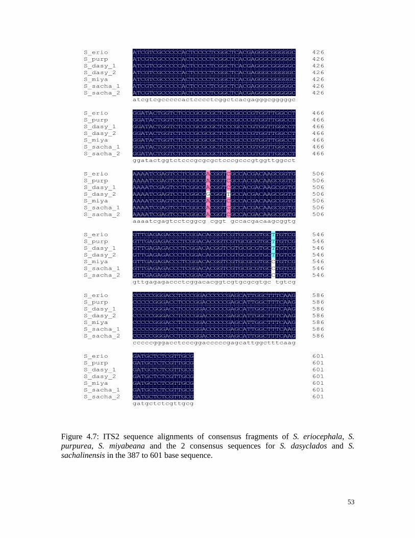
53

426S_erio

426S_purp

426S_dasy_1

426S_dasy_2

426S_miya

426S_sacha_1

426S_sacha_2

ATCGTCGCCCCCACTCCCCTCGGCTCACGAGGGCGGGGGC

ATCGTCGCCCCCACTCCCCTCGGCTCACGAGGGCGGGGGC

ATCGTCGCCCCCACTCCCCTCGGCTCACGAGGGCGGGGGC

ATCGTCGCCCCCACTCCCCTCGGCTCACGAGGGCGGGGGC

ATCGTCGCCCCCACTCCCCTCGGCTCACGAGGGCGGGGGC

ATCGTCGCCCCCACTCCCCTCGGCTCACGAGGGCGGGGGC

ATCGTCGCCCCCACTCCCCTCGGCTCACGAGGGCGGGGGC

a

A

A

A

A

A

A

A

t

T

T

T

T

T

T

T

c

C

C

C

C

C

C

C

g

G

G

G

G

G

G

G

t

T

T

T

T

T

T

T

c

C

C

C

C

C

C

C

g

G

G

G

G

G

G

G

c

C

C

C

C

C

C

C

c

C

C

C

C

C

C

C

c

C

C

C

C

C

C

C

c

C

C

C

C

C

C

C

c

C

C

C

C

C

C

C

a

A

A

A

A

A

A

A

c

C

C

C

C

C

C

C

t

T

T

T

T

T

T

T

c

C

C

C

C

C

C

C

c

C

C

C

C

C

C

C

c

C

C

C

C

C

C

C

c

C

C

C

C

C

C

C

t

T

T

T

T

T

T

T

c

C

C

C

C

C

C

C

g

G

G

G

G

G

G

G

g

G

G

G

G

G

G

G

c

C

C

C

C

C

C

C

t

T

T

T

T

T

T

T

c

C

C

C

C

C

C

C

a

A

A

A

A

A

A

A

c

C

C

C

C

C

C

C

g

G

G

G

G

G

G

G

a

A

A

A

A

A

A

A

g

G

G

G

G

G

G

G

g

G

G

G

G

G

G

G

g

G

G

G

G

G

G

G

c

C

C

C

C

C

C

C

g

G

G

G

G

G

G

G

g

G

G

G

G

G

G

G

g

G

G

G

G

G

G

G

g

G

G

G

G

G

G

G

g

G

G

G

G

G

G

G

c

C

C

C

C

C

C

C

466S_erio

466S_purp

466S_dasy_1

466S_dasy_2

466S_miya

466S_sacha_1

466S_sacha_2

GGATACTGGTCTCCCGCGCGCTCCCGCCCGTGGTTGGCCT

GGATACTGGTCTCCCGCGCGCTCCCGCCCGTGGTTGGCCT

GGATACTGGTCTCCCGCGCGCTCCCGCCCGTGGTTGGCCT

GGATACTGGTCTCCCGCGCGCTCCCGCCCGTGGTTGGCCT

GGATACTGGTCTCCCGCGCGCTCCCGCCCGTGGTTGGCCT

GGATACTGGTCTCCCGCGCGCTCCCGCCCGTGGTTGGCCT

GGATACTGGTCTCCCGCGCGCTCCCGCCCGTGGTTGGCCT

g

G

G

G

G

G

G

G

g

G

G

G

G

G

G

G

a

A

A

A

A

A

A

A

t

T

T

T

T

T

T

T

a

A

A

A

A

A

A

A

c

C

C

C

C

C

C

C

t

T

T

T

T

T

T

T

g

G

G

G

G

G

G

G

g

G

G

G

G

G

G

G

t

T

T

T

T

T

T

T

c

C

C

C

C

C

C

C

t

T

T

T

T

T

T

T

c

C

C

C

C

C

C

C

c

C

C

C

C

C

C

C

c

C

C

C

C

C

C

C

g

G

G

G

G

G

G

G

c

C

C

C

C

C

C

C

g

G

G

G

G

G

G

G

c

C

C

C

C

C

C

C

g

G

G

G

G

G

G

G

c

C

C

C

C

C

C

C

t

T

T

T

T

T

T

T

c

C

C

C

C

C

C

C

c

C

C

C

C

C

C

C

c

C

C

C

C

C

C

C

g

G

G

G

G

G

G

G

c

C

C

C

C

C

C

C

c

C

C

C

C

C

C

C

c

C

C

C

C

C

C

C

g

G

G

G

G

G

G

G

t

T

T

T

T

T

T

T

g

G

G

G

G

G

G

G

g

G

G

G

G

G

G

G

t

T

T

T

T

T

T

T

t

T

T

T

T

T

T

T

g

G

G

G

G

G

G

G

g

G

G

G

G

G

G

G

c

C

C

C

C

C

C

C

c

C

C

C

C

C

C

C

t

T

T

T

T

T

T

T

506S_erio

506S_purp

506S_dasy_1

506S_dasy_2

506S_miya

506S_sacha_1

506S_sacha_2

AAAATCGAGTCCTCGGCGACGGTCGCCACGACAAGCGGTG

AAAATCGAGTCCTCGGCGACGGTCGCCACGACAAGCGGTG

AAAATCGAGTCCTCGGCGACGGTCGCCACGACAAGCGGTG

AAAATCGAGTCCTCGGCGGCGGTTGCCACGACAAGCGGTG

AAAATCGAGTCCTCGGCGACGGTCGCCACGACAAGCGGTG

AAAATCGAGTCCTCGGCGACGGTCGCCACGACAAGCGGTG

AAAATCGAGTCCTCGGCGACGGTCGCCACGACAAGCGGTG

a

A

A

A

A

A

A

A

a

A

A

A

A

A

A

A

a

A

A

A

A

A

A

A

a

A

A

A

A

A

A

A

t

T

T

T

T

T

T

T

c

C

C

C

C

C

C

C

g

G

G

G

G

G

G

G

a

A

A

A

A

A

A

A

g

G

G

G

G

G

G

G

t

T

T

T

T

T

T

T

c

C

C

C

C

C

C

C

c

C

C

C

C

C

C

C

t

T

T

T

T

T

T

T

c

C

C

C

C

C

C

C

g

G

G

G

G

G

G

G

g

G

G

G

G

G

G

G

c

C

C

C

C

C

C

C

g

G

G

G

G

G

G

G

A

A

A

A

A

A

c

C

C

C

C

C

C

C

g

G

G

G

G

G

G

G

g

G

G

G

G

G

G

G

t

T

T

T

T

T

T

T

C

C

C

C

C

C

g

G

G

G

G

G

G

G

c

C

C

C

C

C

C

C

c

C

C

C

C

C

C

C

a

A

A

A

A

A

A

A

c

C

C

C

C

C

C

C

g

G

G

G

G

G

G

G

a

A

A

A

A

A

A

A

c

C

C

C

C

C

C

C

a

A

A

A

A

A

A

A

a

A

A

A

A

A

A

A

g

G

G

G

G

G

G

G

c

C

C

C

C

C

C

C

g

G

G

G

G

G

G

G

g

G

G

G

G

G

G

G

t

T

T

T

T

T

T

T

g

G

G

G

G

G

G

G

546S_erio

546S_purp

546S_dasy_1

546S_dasy_2

546S_miya

546S_sacha_1

546S_sacha_2

GTTGAGAGACCCTCGGACACGGTCGTGCGCGTGCTTGTCG

GTTGAGAGACCCTCGGACACGGTCGTGCGCGTGCTTGTCG

GTTGAGAGACCCTCGGACACGGTCGTGCGCGTGCTTGTCG

GTTGAGAGACCCTCGGACACGGTCGTGCGCGTGCTTGTCG

GTTGAGAGACCCTCGGACACGGTCGTGCGCGTGCCTGTCG

GTTGAGAGACCCTCGGACACGGTCGTGCGCGTGCCTGTCG

GTTGAGAGACCCTCGGACACGGTCGTGCGCGTGCCTGTCG

g

G

G

G

G

G

G

G

t

T

T

T

T

T

T

T

t

T

T

T

T

T

T

T

g

G

G

G

G

G

G

G

a

A

A

A

A

A

A

A

g

G

G

G

G

G

G

G

a

A

A

A

A

A

A

A

g

G

G

G

G

G

G

G

a

A

A

A

A

A

A

A

c

C

C

C

C

C

C

C

c

C

C

C

C

C

C

C

c

C

C

C

C

C

C

C

t

T

T

T

T

T

T

T

c

C

C

C

C

C

C

C

g

G

G

G

G

G

G

G

g

G

G

G

G

G

G

G

a

A

A

A

A

A

A

A

c

C

C

C

C

C

C

C

a

A

A

A

A

A

A

A

c

C

C

C

C

C

C

C

g

G

G

G

G

G

G

G

g

G

G

G

G

G

G

G

t

T

T

T

T

T

T

T

c

C

C

C

C

C

C

C

g

G

G

G

G

G

G

G

t

T

T

T

T

T

T

T

g

G

G

G

G

G

G

G

c

C

C

C

C

C

C

C

g

G

G

G

G

G

G

G

c

C

C

C

C

C

C

C

g

G

G

G

G

G

G

G

t

T

T

T

T

T

T

T

g

G

G

G

G

G

G

G

c

C

C

C

C

C

C

C

T

T

T

T

t

T

T

T

T

T

T

T

g

G

G

G

G

G

G

G

t

T

T

T

T

T

T

T

c

C

C

C

C

C

C

C

g

G

G

G

G

G

G

G

586S_erio

586S_purp

586S_dasy_1

586S_dasy_2

586S_miya

586S_sacha_1

586S_sacha_2

CCCCCGGGACCTCCCGGACCCCCGAGCATTGGCTTTCAAG

CCCCCGGGACCTCCCGGACCCCCGAGCATTGGCTTTCAAG

CCCCCGGGACCTCCCGGACCCCCGAGCATTGGCTTTCAAG

CCCCCGGGACCTCCCGGACCCCCGAGCATTGGCTTTCAAG

CCCCCGGGACCTCCCGGACCCCCGAGCATTGGCTTTCAAG

CCCCCGGGACCTCCCGGACCCCCGAGCATTGGCTTTCAAG

CCCCCGGGACCTCCCGGACCCCCGAGCATTGGCTTTCAAG

c

C

C

C

C

C

C

C

c

C

C

C

C

C

C

C

c

C

C

C

C

C

C

C

c

C

C

C

C

C

C

C

c

C

C

C

C

C

C

C

g

G

G

G

G

G

G

G

g

G

G

G

G

G

G

G

g

G

G

G

G

G

G

G

a

A

A

A

A

A

A

A

c

C

C

C

C

C

C

C

c

C

C

C

C

C

C

C

t

T

T

T

T

T

T

T

c

C

C

C

C

C

C

C

c

C

C

C

C

C

C

C

c

C

C

C

C

C

C

C

g

G

G

G

G

G

G

G

g

G

G

G

G

G

G

G

a

A

A

A

A

A

A

A

c

C

C

C

C

C

C

C

c

C

C

C

C

C

C

C

c

C

C

C

C

C

C

C

c

C

C

C

C

C

C

C

c

C

C

C

C

C

C

C

g

G

G

G

G

G

G

G

a

A

A

A

A

A

A

A

g

G

G

G

G

G

G

G

c

C

C

C

C

C

C

C

a

A

A

A

A

A

A

A

t

T

T

T

T

T

T

T

t

T

T

T

T

T

T

T

g

G

G

G

G

G

G

G

g

G

G

G

G

G

G

G

c

C

C

C

C

C

C

C

t

T

T

T

T

T

T

T

t

T

T

T

T

T

T

T

t

T

T

T

T

T

T

T

c

C

C

C

C

C

C

C

a

A

A

A

A

A

A

A

a

A

A

A

A

A

A

A

g

G

G

G

G

G

G

G

601S_erio

601S_purp

601S_dasy_1

601S_dasy_2

601S_miya

601S_sacha_1

601S_sacha_2

GATGCTCTCGTTGCG

GATGCTCTCGTTGCG

GATGCTCTCGTTGCG

GATGCTCTCGTTGCG

GATGCTCTCGTTGCG

GATGCTCTCGTTGCG

GATGCTCTCGTTGCG

g

G

G

G

G

G

G

G

a

A

A

A

A

A

A

A

t

T

T

T

T

T

T

T

g

G

G

G

G

G

G

G

c

C

C

C

C

C

C

C

t

T

T

T

T

T

T

T

c

C

C

C

C

C

C

C

t

T

T

T

T

T

T

T

c

C

C

C

C

C

C

C

g

G

G

G

G

G

G

G

t

T

T

T

T

T

T

T

t

T

T

T

T

T

T

T

g

G

G

G

G

G

G

G

c

C

C

C

C

C

C

C

g

G

G

G

G

G

G

G

Figure 4.7: ITS2 sequence alignments of consensus fragments of S. eriocephala, S.

purpurea, S. miyabeana and the 2 consensus sequences for S. dasyclados and S.

sachalinensis in the 387 to 601 base sequence.

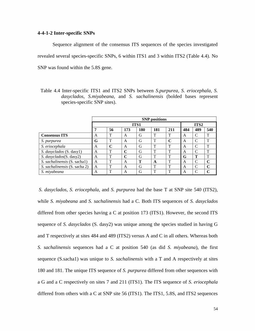
54

4-4-1-2 Inter-specific SNPs

Sequence alignment of the consensus ITS sequences of the species investigated

revealed several species-specific SNPs, 6 within ITS1 and 3 within ITS2 (Table 4.4). No

SNP was found within the 5.8S gene.

Table 4.4 Inter-specific ITS1 and ITS2 SNPs between S.purpurea, S. eriocephala, S.

dasyclados, S.miyabeana, and S. sachalinensis (bolded bases represent

species-specific SNP sites).

SNP positions

ITS1 ITS2

7 56 173 180 181 211 484 489 540

Consensus ITS A T A G T T A C T

S. purpurea G T A G T C A C T

S. eriocephala A C A G T T A C T

S. dasyclados (S. dasy1) A T C G T T A C T

S. dasyclados(S. dasy2) A T C G T T G T T

S. sachalinensis (S. sacha1) A T A T A T A C C

S. sachalinensis (S. sacha 2) A T A G T T A C C

S. miyabeana A T A G T T A C C

S. dasyclados, S. eriocephala, and S. purpurea had the base T at SNP site 540 (ITS2),

while S. miyabeana and S. sachalinensis had a C. Both ITS sequences of S. dasyclados

differed from other species having a C at position 173 (ITS1). However, the second ITS

sequence of S. dasyclados (S. dasy2) was unique among the species studied in having G

and T respectively at sites 484 and 489 (ITS2) versus A and C in all others. Whereas both

S. sachalinensis sequences had a C at position 540 (as did S. miyabeana), the first

sequence (S.sacha1) was unique to S. sachalinensis with a T and A respectively at sites

180 and 181. The unique ITS sequence of S. purpurea differed from other sequences with

a G and a C respectively on sites 7 and 211 (ITS1). The ITS sequence of S. eriocephala

differed from others with a C at SNP site 56 (ITS1). The ITS1, 5.8S, and ITS2 sequences

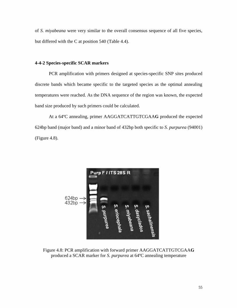
55

of S. miyabeana were very similar to the overall consensus sequence of all five species,

but differed with the C at position 540 (Table 4.4).

4-4-2 Species-specific SCAR markers

PCR amplification with primers designed at species-specific SNP sites produced

discrete bands which became specific to the targeted species as the optimal annealing

temperatures were reached. As the DNA sequence of the region was known, the expected

band size produced by such primers could be calculated.

At a 64ºC annealing, primer AAGGATCATTGTCGAAG produced the expected

624bp band (major band) and a minor band of 432bp both specific to S. purpurea (94001)

(Figure 4.8).

Figure 4.8: PCR amplification with forward primer AAGGATCATTGTCGAAG

produced a SCAR marker for S. purpurea at 64ºC annealing temperature

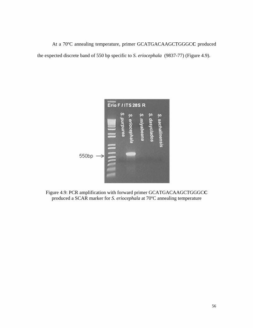
56

At a 70ºC annealing temperature, primer GCATGACAAGCTGGGCC produced

the expected discrete band of 550 bp specific to S. eriocephala (9837-77) (Figure 4.9).

Figure 4.9: PCR amplification with forward primer GCATGACAAGCTGGGCC

produced a SCAR marker for S. eriocephala at 70ºC annealing temperature

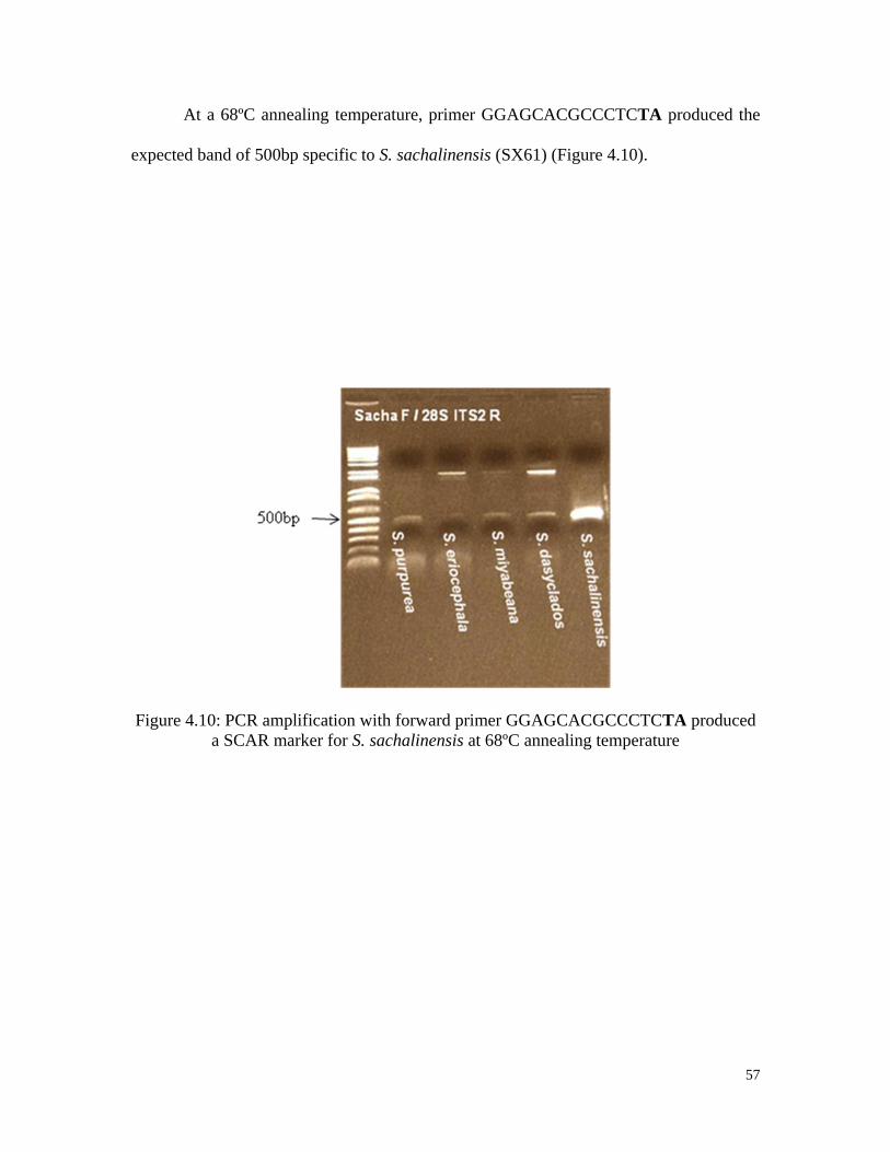
57

At a 68ºC annealing temperature, primer GGAGCACGCCCTCTA produced the

expected band of 500bp specific to S. sachalinensis (SX61) (Figure 4.10).

Figure 4.10: PCR amplification with forward primer GGAGCACGCCCTCTA produced

a SCAR marker for S. sachalinensis at 68ºC annealing temperature

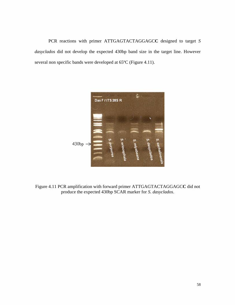
58

PCR reactions with primer ATTGAGTACTAGGAGCC designed to target S

dasyclados did not develop the expected 430bp band size in the target line. However

several non specific bands were developed at 65ºC (Figure 4.11).

Figure 4.11 PCR amplification with forward primer ATTGAGTACTAGGAGCC did not

produce the expected 430bp SCAR marker for S. dasyclados.

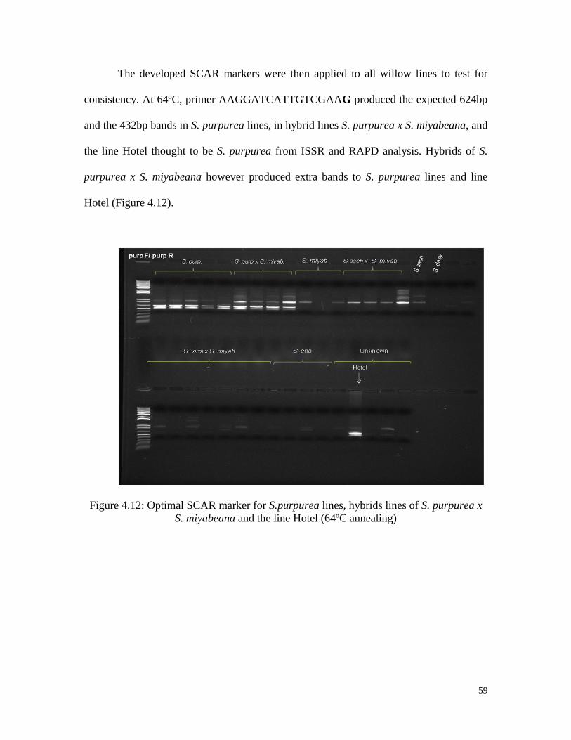
59

The developed SCAR markers were then applied to all willow lines to test for

consistency. At 64ºC, primer AAGGATCATTGTCGAAG produced the expected 624bp

and the 432bp bands in S. purpurea lines, in hybrid lines S. purpurea x S. miyabeana, and

the line Hotel thought to be S. purpurea from ISSR and RAPD analysis. Hybrids of S.

purpurea x S. miyabeana however produced extra bands to S. purpurea lines and line

Hotel (Figure 4.12).

Figure 4.12: Optimal SCAR marker for S.purpurea lines, hybrids lines of S. purpurea x

S. miyabeana and the line Hotel (64ºC annealing)

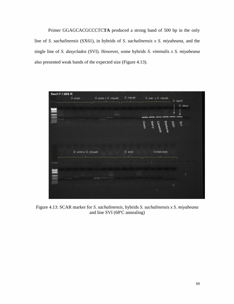
60

Primer GGAGCACGCCCTCTA produced a strong band of 500 bp in the only

line of S. sachalinensis (SX61), in hybrids of S. sachalinensis x S. miyabeana, and the

single line of S. dasyclados (SVI). However, some hybrids S. viminalis x S. miyabeana

also presented weak bands of the expected size (Figure 4.13).

Figure 4.13: SCAR marker for S. sachalinensis, hybrids S. sachalinensis x S. miyabeana

and line SVI (68ºC annealing)

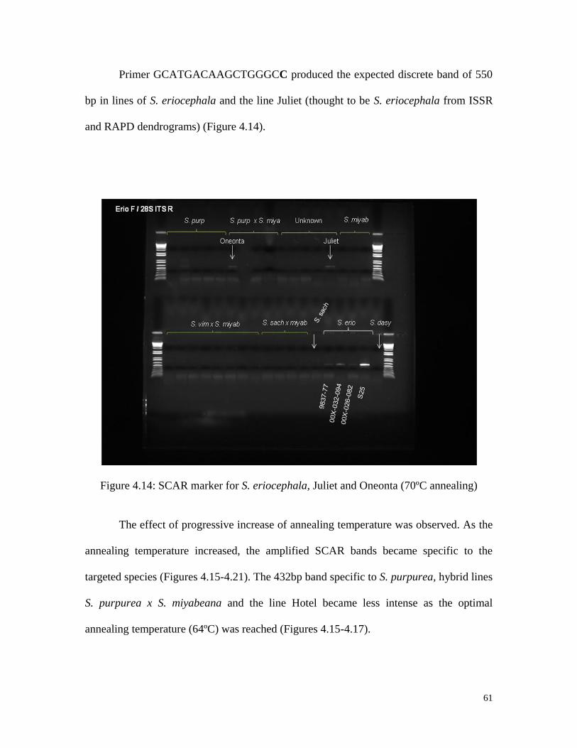
61

Primer GCATGACAAGCTGGGCC produced the expected discrete band of 550

bp in lines of S. eriocephala and the line Juliet (thought to be S. eriocephala from ISSR

and RAPD dendrograms) (Figure 4.14).

Figure 4.14: SCAR marker for S. eriocephala, Juliet and Oneonta (70ºC annealing)

The effect of progressive increase of annealing temperature was observed. As the

annealing temperature increased, the amplified SCAR bands became specific to the

targeted species (Figures 4.15-4.21). The 432bp band specific to S. purpurea, hybrid lines

S. purpurea x S. miyabeana and the line Hotel became less intense as the optimal

annealing temperature (64ºC) was reached (Figures 4.15-4.17).

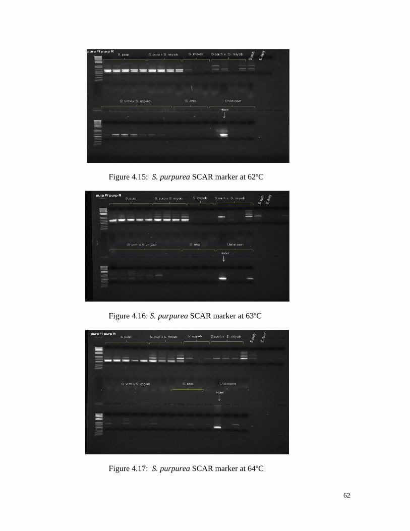
62

Figure 4.15: S. purpurea SCAR marker at 62ºC

Figure 4.16: S. purpurea SCAR marker at 63ºC

Figure 4.17: S. purpurea SCAR marker at 64ºC

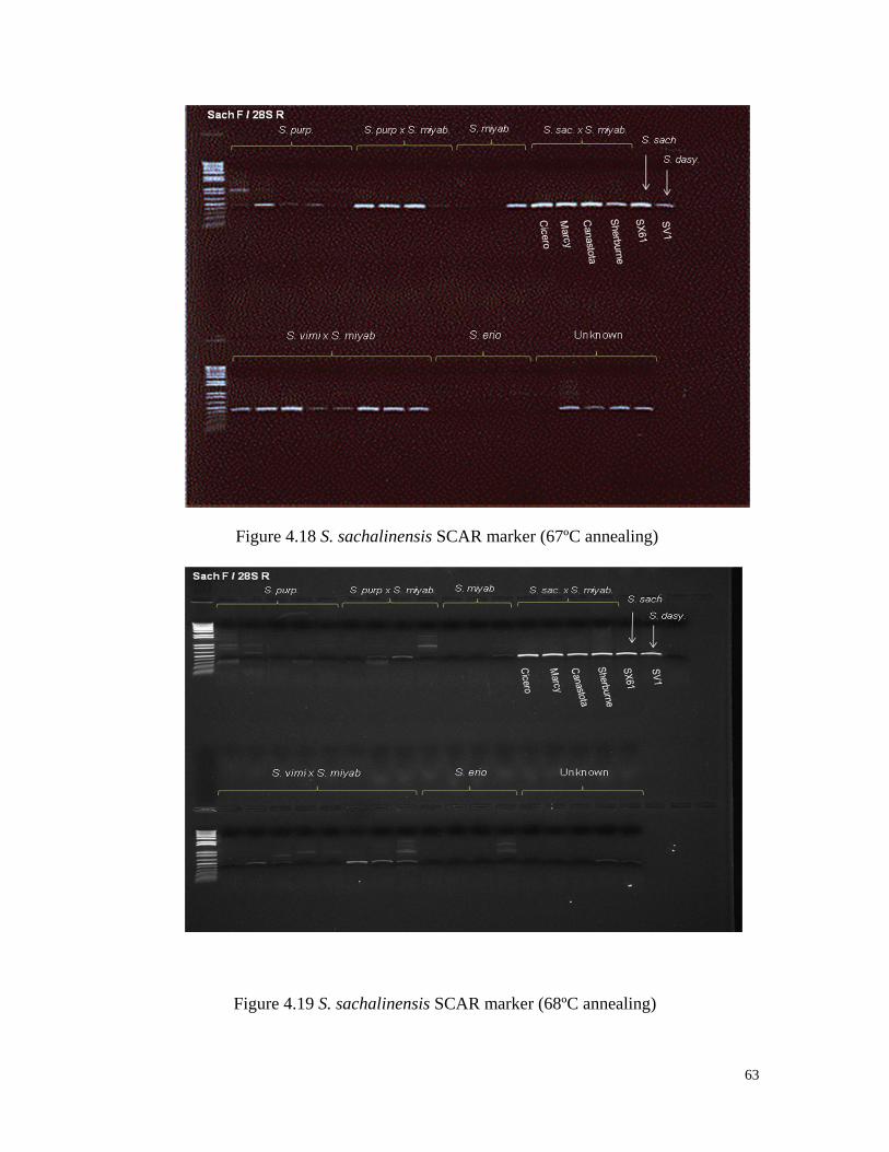
63

Figure 4.18 S. sachalinensis SCAR marker (67ºC annealing)

Figure 4.19 S. sachalinensis SCAR marker (68ºC annealing)

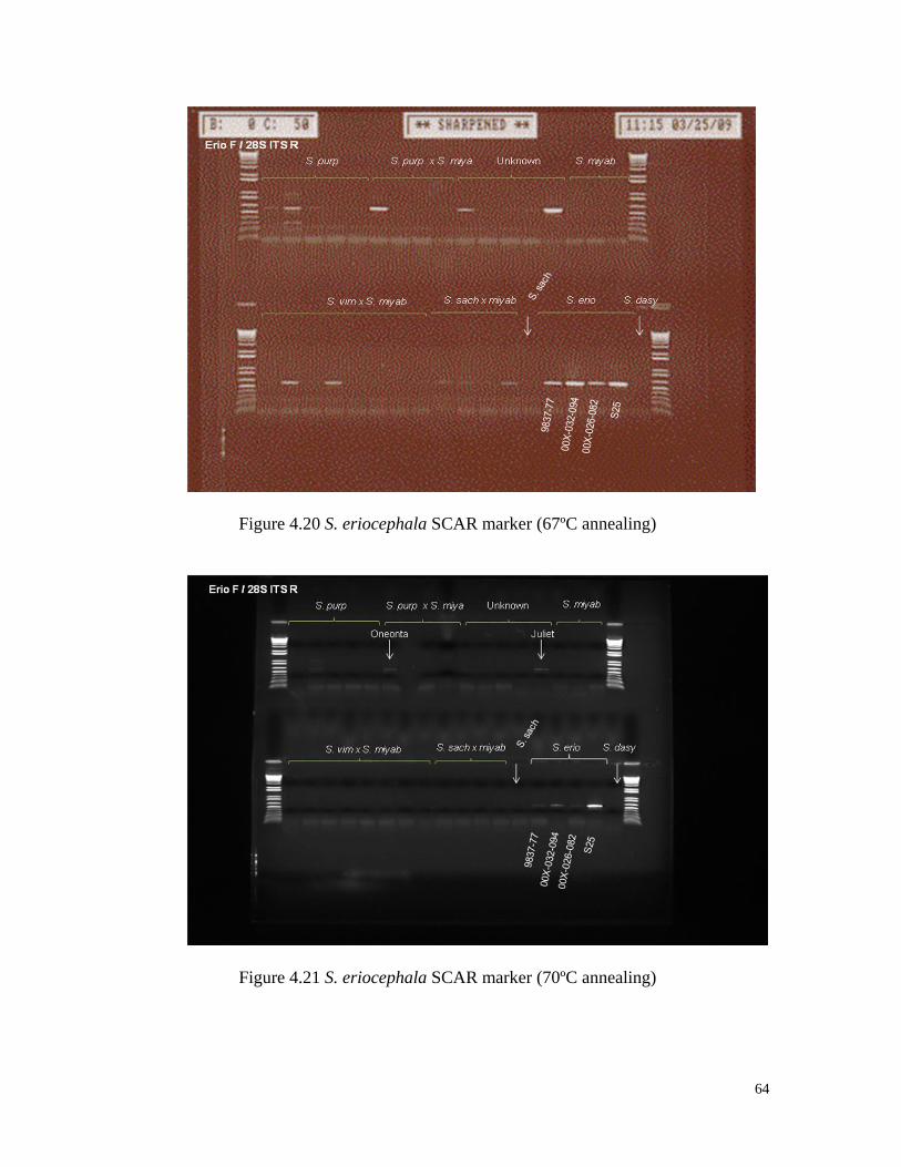
64

Figure 4.20 S. eriocephala SCAR marker (67ºC annealing)

Figure 4.21 S. eriocephala SCAR marker (70ºC annealing)

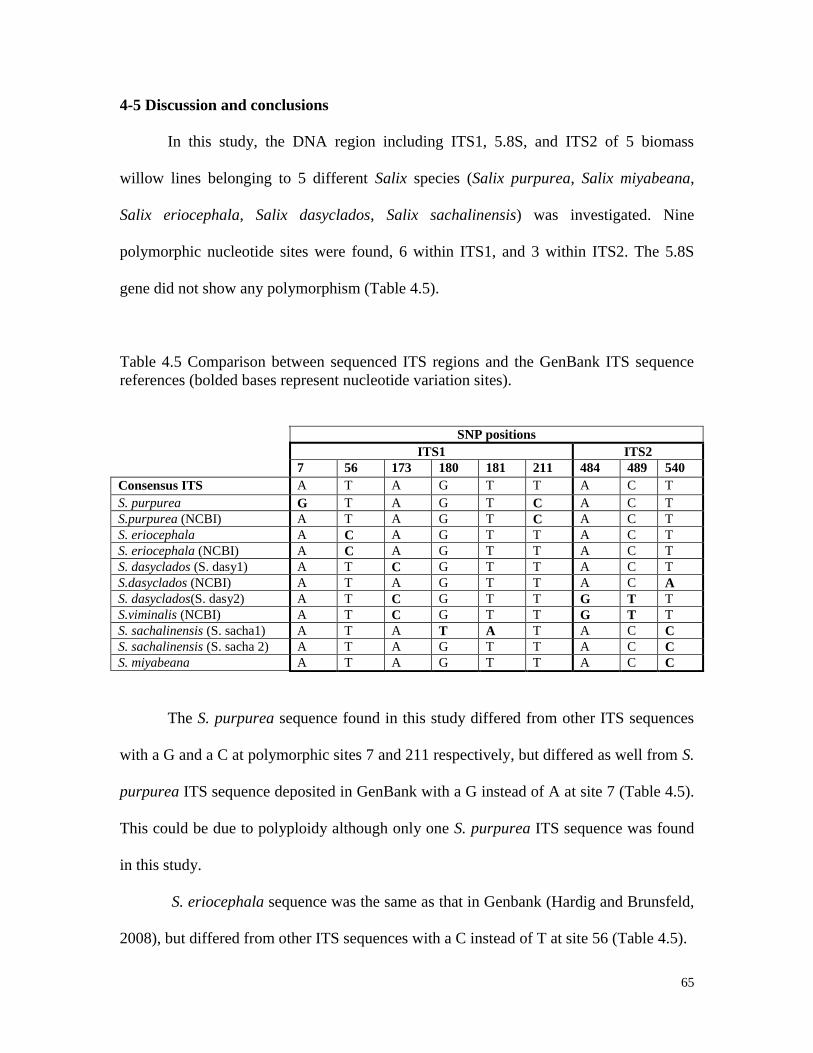
65

4-5 Discussion and conclusions

In this study, the DNA region including ITS1, 5.8S, and ITS2 of 5 biomass

willow lines belonging to 5 different Salix species (Salix purpurea, Salix miyabeana,

Salix eriocephala, Salix dasyclados, Salix sachalinensis) was investigated. Nine

polymorphic nucleotide sites were found, 6 within ITS1, and 3 within ITS2. The 5.8S

gene did not show any polymorphism (Table 4.5).

Table 4.5 Comparison between sequenced ITS regions and the GenBank ITS sequence

references (bolded bases represent nucleotide variation sites).

SNP positions

ITS1 ITS2

7 56 173 180 181 211 484 489 540

Consensus ITS A T A G T T A C T

S. purpurea G T A G T C A C T

S.purpurea (NCBI) A T A G T C A C T

S. eriocephala A C A G T T A C T

S. eriocephala (NCBI) A C A G T T A C T

S. dasyclados (S. dasy1) A T C G T T A C T

S.dasyclados (NCBI) A T A G T T A C A

S. dasyclados(S. dasy2) A T C G T T G T T

S.viminalis (NCBI) A T C G T T G T T

S. sachalinensis (S. sacha1) A T A T A T A C C

S. sachalinensis (S. sacha 2) A T A G T T A C C

S. miyabeana A T A G T T A C C

The S. purpurea sequence found in this study differed from other ITS sequences

with a G and a C at polymorphic sites 7 and 211 respectively, but differed as well from S.

purpurea ITS sequence deposited in GenBank with a G instead of A at site 7 (Table 4.5).

This could be due to polyploidy although only one S. purpurea ITS sequence was found

in this study.

S. eriocephala sequence was the same as that in Genbank (Hardig and Brunsfeld,

2008), but differed from other ITS sequences with a C instead of T at site 56 (Table 4.5).

66

Three polymorphic nucleotide sites were found within ITS clones of S.

dasyclados, leading to the identification of 2 ITS fragments. The first fragment (S. dasy1)

had a C, a A and a C respectively on sites 173, 484 and 489, whereas the second (S.

dasy2) had a C, a G and a T respectively. The second S. dasyclados fragment was the

same as S. viminalis ITS sequence in Genbank (Leskinen and Alstron, 1999) (Table 4.5).

This was an indication that either S. dasyclados or S. viminalis could be closely related,

or a sign of a possible introgression of S. viminalis into the S. dasyclados genome. The

first S. dasyclados ITS fragment (S. dasy1) was closer to the GenBank S. dasyclados ITS

sequence (Leskinen and Alstron, 1999) (Table 4.5), but differed at site 173 and 540

where a C was found instead of an A, and a T instead of an A respectively (Table 4.5).

Two polymorphic nucleotide sites were found within ITS clones of S.

sachalinensis, leading to the identification of two ITS fragments differing at sites 180 and

181. The first fragment had T and A, and the second fragment had G and T respectively

(Table 4.5). Fragment 1 (S. sacha1) was unique to S. sachalinensis and was not found in

any other published ITS sequence of Salix and Populus species (Leskinen and Alstron,

1999). The second fragment (S. sacha2) was much closer to the ITS sequences of S.

miyabeana (Table 4.5). The presence of two rRNA loci could be an indication of the

polyploidy of the investigated S. sachalinensis line. No S. sachalinensis ITS sequence has

been published in GenBank.

The ITS sequence of S. miyabeana was identical to the overall consensus ITS

sequence of the investigated Salix species (Table 4.5). No ITS sequence of S. miyabeana

has been published.

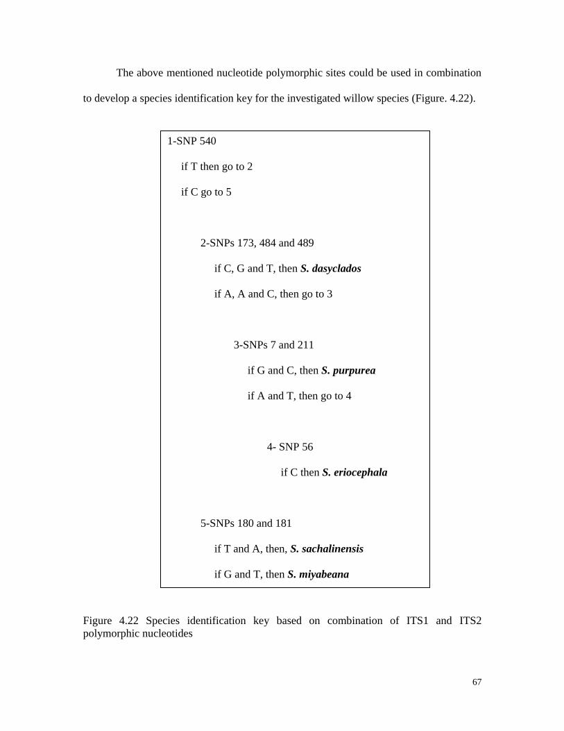
67

The above mentioned nucleotide polymorphic sites could be used in combination

to develop a species identification key for the investigated willow species (Figure. 4.22).

Figure 4.22 Species identification key based on combination of ITS1 and ITS2

polymorphic nucleotides

1-SNP 540

if T then go to 2

if C go to 5

2-SNPs 173, 484 and 489

if C, G and T, then S. dasyclados

if A, A and C, then go to 3

3-SNPs 7 and 211

if G and C, then S. purpurea

if A and T, then go to 4

4- SNP 56

if C then S. eriocephala

5-SNPs 180 and 181

if T and A, then, S. sachalinensis

if G and T, then S. miyabeana

68

5- GENERAL DISCUSSION AND CONCLUSION

The dendrograms developed from RAPD and ISSR markers grouped different

species and hybrids in clusters. The differences of banding patterns were used for the

identification of willow lines. This confirms the efficiency of ISSR and RAPD marker

techniques for genetic diversity analysis and for identification within Salicaceae reported

by many authors (Rajora and Rahman, 2003; Gao et al., 2006; Sulima et al., 2009).

The determination of the total nuclear DNA content of different lines helped to

confirm the groupings of species and hybrids observed on the dendrograms, and

confirmed as well the correlations between nuclear DNA contents of hybrid and parental

lines. The observed variability in ploidy levels within and between species have been

reported in previous investigations on ploidy levels within the genus Salix (Suda and

Argus, 1968; Thibault, 1998).

The analysis of rRNA gene regions including ITS1, 5.8S gene and ITS2 were

useful for the identification of intra- and inter-specific nucleotide polymorphisms. Inter-

and intra-species heterogeneity has been reported in many plants species (Saini et al.,

2008; Hillis, 1988). The amplified ITS sequences were very similar to Salix ITS

sequences published in GenBank (Leskinen and Alstron, 1999; Hardig and Brunsfeld,

2008).

The developed SCAR markers contributed to confirming the observed species-

specific SNPs, as well as the species names of some lines of unknown origins. They

appeared to be quicker to perform, easier to use and less expensive compared to SNP

markers which necessitated PCR amplification, sequencing and sequence alignments.

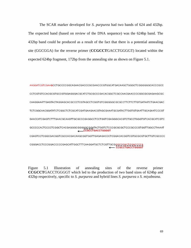
69

The SCAR marker developed for S. purpurea had two bands of 624 and 432bp.

The expected band (based on review of the DNA sequence) was the 624bp band. The

432bp band could be produced as a result of the fact that there is a potential annealing

site (GGCGGA) for the reverse primer (CCGCCTGACCTGGGGT) located within the

expected 624bp fragment, 172bp from the annealing site as shown on Figure 5.1.

Figure 5.1 Illustration of annealing sites of the reverse primer

CCGCCTGACCTGGGGT which led to the production of two band sizes of 624bp and

432bp respectively, specific to S. purpurea and hybrid lines S. purpurea x S. miyabeana.

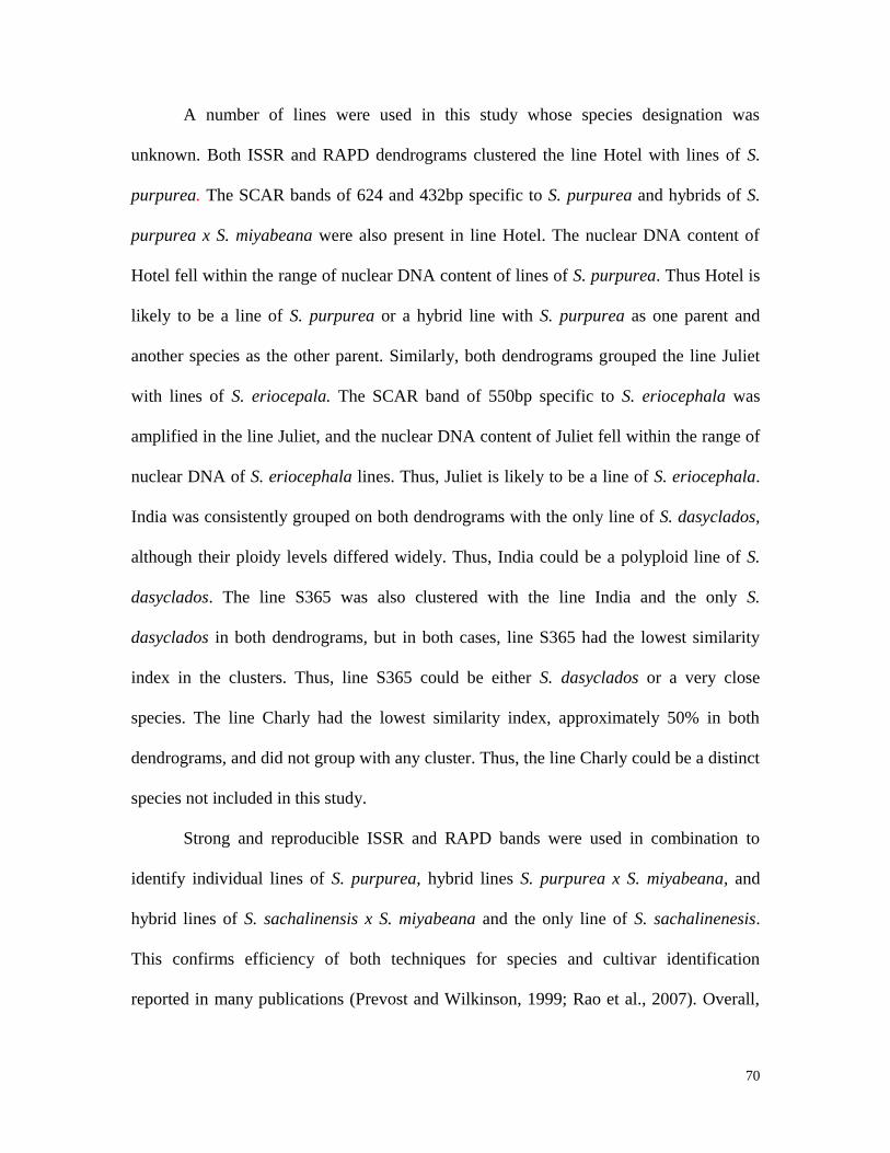
70

A number of lines were used in this study whose species designation was

unknown. Both ISSR and RAPD dendrograms clustered the line Hotel with lines of S.

purpurea. The SCAR bands of 624 and 432bp specific to S. purpurea and hybrids of S.

purpurea x S. miyabeana were also present in line Hotel. The nuclear DNA content of

Hotel fell within the range of nuclear DNA content of lines of S. purpurea. Thus Hotel is

likely to be a line of S. purpurea or a hybrid line with S. purpurea as one parent and

another species as the other parent. Similarly, both dendrograms grouped the line Juliet

with lines of S. eriocepala. The SCAR band of 550bp specific to S. eriocephala was

amplified in the line Juliet, and the nuclear DNA content of Juliet fell within the range of

nuclear DNA of S. eriocephala lines. Thus, Juliet is likely to be a line of S. eriocephala.

India was consistently grouped on both dendrograms with the only line of S. dasyclados,

although their ploidy levels differed widely. Thus, India could be a polyploid line of S.

dasyclados. The line S365 was also clustered with the line India and the only S.

dasyclados in both dendrograms, but in both cases, line S365 had the lowest similarity

index in the clusters. Thus, line S365 could be either S. dasyclados or a very close

species. The line Charly had the lowest similarity index, approximately 50% in both

dendrograms, and did not group with any cluster. Thus, the line Charly could be a distinct

species not included in this study.

Strong and reproducible ISSR and RAPD bands were used in combination to

identify individual lines of S. purpurea, hybrid lines S. purpurea x S. miyabeana, and

hybrid lines of S. sachalinensis x S. miyabeana and the only line of S. sachalinenesis.

This confirms efficiency of both techniques for species and cultivar identification

reported in many publications (Prevost and Wilkinson, 1999; Rao et al., 2007). Overall,

71

the evaluation of 2C nuclear DNA through flow cytometry, ITS analysis, ISSR / RAPD

markers were effective in revealing genetic diversity and to fingerprint willow species

and lines used in the program.

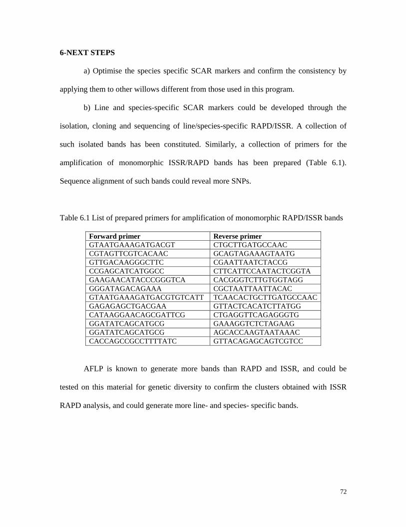
72

6-NEXT STEPS

a) Optimise the species specific SCAR markers and confirm the consistency by

applying them to other willows different from those used in this program.

b) Line and species-specific SCAR markers could be developed through the

isolation, cloning and sequencing of line/species-specific RAPD/ISSR. A collection of

such isolated bands has been constituted. Similarly, a collection of primers for the

amplification of monomorphic ISSR/RAPD bands has been prepared (Table 6.1).

Sequence alignment of such bands could reveal more SNPs.

Table 6.1 List of prepared primers for amplification of monomorphic RAPD/ISSR bands

Forward primer Reverse primer

GTAATGAAAGATGACGT CTGCTTGATGCCAAC

CGTAGTTCGTCACAAC GCAGTAGAAAGTAATG

GTTGACAAGGGCTTC CGAATTAATCTACCG

CCGAGCATCATGGCC CTTCATTCCAATACTCGGTA

GAAGAACATACCCGGGTCA CACGGGTCTTGTGGTAGG

GGGATAGACAGAAA CGCTAATTAATTACAC

GTAATGAAAGATGACGTGTCATT TCAACACTGCTTGATGCCAAC

GAGAGAGCTGACGAA GTTACTCACATCTTATGG

CATAAGGAACAGCGATTCG CTGAGGTTCAGAGGGTG

GGATATCAGCATGCG GAAAGGTCTCTAGAAG

GGATATCAGCATGCG AGCACCAAGTAATAAAC

CACCAGCCGCCTTTTATC GTTACAGAGCAGTCGTCC

AFLP is known to generate more bands than RAPD and ISSR, and could be

tested on this material for genetic diversity to confirm the clusters obtained with ISSR

RAPD analysis, and could generate more line- and species- specific bands.

73

7- REFERENCES

Abrahamson, L.P., Robison, D.J., Volk, T.A., White, E.H., Neuhauser, E.F.,

Benjamin, W.H. and Peterson, J.M. (1998). Sustainability and environmental issues

associated with willow bioenergy development in New York (USA). Biomass Bioenergy,

15(1):17-22.

Achard, F., Eva, H.D., Stibig, H.-J., Mayaux, P., Gallego, J., Richards, T. and

Malingreau, J.-P. (2002). Determination of deforestation rates of the world’s humid

tropical forests. Science, 297:999-1002.

Argus, G.W. (1986). The genus Salix (Salicaceae) in the southeastern United

States. Syst. Bot. Monogr., 9:1-170.

Argus, G.W. (1997). Intra-generic classification of Salix in the New World. Syst.

Bot. Monogr., 52:1-121.

Arumuganathan, K. and Earle, E.D. (1991). Estimation of nuclear DNA content

of plants by flow cytometry. Plant Molecular Biology Reporter, 9: 229-241.

Baldwin, B.G. (1992). Phylogenetic utility of the internal transcribed spacers of

nuclear ribosomal DNA in plants: an example from the Compositeae. Mol. Phylogenet.

Evol., 1:3-16.

Barker, J.H.A., Pahlich, A., Trybush, S., Edwards, K.J. and Karp, A. (2003).

Microsatellite markers for diverse Salix species Mol. Ecol. Notes, 3: 4-6.

Barker, J.H.A., Matthes, M., Arnold, M.G., Edwards, K.J., Åhman, I., Larsson,S.

and Karp, A. (1999). Characterisation of genetic diversity in potential biomass willows

(Salix spp.) by RAPD and AFLP analysis. Genome, 42:173-183.

Beckmann, J. and Soller, M. (1986). Restriction fragment length polymorphisms

in plant genetic improvement. Oxford. Surv. Plant Mol. Cell Biol. 3:197-250.

Bennett, M.D. (1985). Intraspecific variation in DNA amount and the nucleotypic

dimension in plant genetics. in Plant Genetics. UCLA Symposia on Molecular and

Cellular Biology. Alan R. Liss, Inc., New York. pp. 283.302.

Bennett, M.D. and Leitch, I.J. (2005). Plant DNA C-values database

http://www.kew.org/cvalues/ (2.01.2010)

Bennewitz, J. (2009). Climate, entropy and environment. Environ. Dev. Sustain.,

11:127-136.

Benning, C. and Pichersky, E. (2008). Harnessing plant biomass for biofuels and

biomaterials. Plant J., 54:533-535.

74

Berndes, G., Hoogwijk, M. and Van den Broek, R. (2003). The contribution of

biomass in the future global energy system: A review of 17 studies. Biomass Bioenergy,

25:1-28.

Bidini, G., Desideri, U. and Fantozzi, F. (2003). Distributed generation of

electricity from biomass using pyrolysis technology. Woody Energy 1:35-37.

Castiglione, S., Wang, G., Damiani, G., Bandi, C., Bisoffi, S. and Sala, F. (1993).

RAPD fingerprints for identification and for taxonomic studies of elite poplar (Populus

spp.) clones. Theor. Appl. Genet., 87:54-59.

Chen,Y-C., Eisner, J. D., Kattar, M. M., Rassoulian-Barrett, S. L., Lafe, K.,

Limaye, A. P. and Cookson, B. P. (2001). Polymorphic internal transcribed spacer region

1 DNA sequences identify medically important yeasts. J. Clin. Microbiol., 39:4042-4051.

Chmelar, J. (1979). The taxonomic importance of chromosome numbers in the

genus Salix L. [In Czech.]. Lesnictví., 25:411-415.

Collard, B.C.Y., Jahufer M.Z.Z., Brouwer J.B. and Pang, E.C.K. (2005). An

introduction to markers, quantitative trait loci (QTL) mapping and marker-assisted

selection for crop improvement: The basic concepts. Euphytica, 142:169-196

Crawford, D. J. (1990). Plant molecular systematic. John Wiley and Sons (eds.),

New York. 388pp.

Darlington, C.D. and Wylie, A.P. (1961) Chromosome atlas of flowering plants.

Hafner, New York, NY, USA. pp. 178-179.

Doebley, J. and Wendel, J.F. (1989). Application of RFLPs to plant systematics.

In: Helentjaris, T. and Burr, B. (eds.) current communications in molecular biology -

development and application of molecular markers to problems in plant genetics. Cold

Spring Harbor Laboratory Press, New York, pp 57-68.

Doležel, J. and Bartos, J. (2005). Plant DNA flow cytometry and estimation of

nuclear genome size. Ann. Bot., 95:99-110.

Dorn, R. D. (1976). A synopsis of American Salix. Can. J. Bot., 54:2769-2789.

Downie, R. and Downie, K.D.S. (1996). A molecular phylogeny of Apiaceae

subfamily Apioideae: Evidence from nuclear ribosomal DNA internal transcribed spacer

sequences. Am. J. Bot., 2:234-251.

Dumbleton, F. (1997). Biomass conversion technologies. An overview. Asp.

Appl. Biol, 49:341-347.

75

Eckstein, P. E., Krasichynska, N., Voth, D., Duncan, S., Rossnagel, B. G. and

Scoles, G. J. (2002). Development of PCR-based markers for a gene (Un8) conferring

true loose smut resistance in barley. Can. J. Plant Pathol., 24:46-53.

Flavell, R.B. (1986). Structure and control of expression of ribosomal RNA

genes. Oxf. Surv. Plant Mol. Cell. Biol., 3:252-274.

Felsenstein, J. (1988). Phylogenies from molecular sequences: inference and

reliability. Ann. Rev. Genet., 22:521-565

Gaiser, L.O. (1930). Chromosome numbers in angiosperms III. Genetica, 12:161-

261.

Gao, J., Zhang, S., Zhang, Y., Wang, C., Song, W. and Han, S. (2006).

Application of ISSR markers to fingerprinting of elite cultivars (varieties/clones) from

different sections of the genus Populus L. Silvae Genet., 55:1-6.

Graham, R. L., Wright, L. L. and Turhollow, A. F. (1992). The potential for short-

rotation woody crops to reduce U.S. CO 2 emissions. Climatic Change, 22: 223-238.

Grogan, P. and Matthews, R. B. (2002). A modelling analysis of the potential for

soil carbon sequestration under short rotation coppice willow bioenergy plantations. Soil

Use and Management, 18:175-183.

Hadrys, H., Balick, M. and Schierwater, B. (1992). Applications of random

amplified polymorphic DNA (RAPD) in molecular ecology. Mol. Ecol., 1:55-63.

Håkansson, A. (1955). Chromosome numbers and meiosis in certain salices.

Hereditas, 41:454-482.

Hanley, S., Barker, J.H.A., Van Ooijen, J.W., Aldam, C., Harris, S.L., Ahman, I.,

Larsson, S. and Karp, A. (2002). A genetic linkage map of willow (Salix viminalis) based

on AFLP and microsatellite markers. Theor. Appl. Genet., 105:1087-1096.

Hardig, T.M. and Brunsfeld, S.J. (2008). A phylogenetic analysis of Salix

(Salicaceae) based on matK and ribosomal DNA sequence data. Forest Resources,

unpublished: sourced from NCBI.

http://www.ncbi.nlm.nih.gov/nuccore/EU784077.1?ordinalpos=2&itool=EntrezSystem2.

PEntrez.Sequence.Sequence_ResultsPanel.Sequence_RVDocSum (22.12.2009).

Hautala, R.R., King, R.B. and Kutal, C. (1979). Solar energy: Chemical

conversion and storage. Humana Press., pp. 333-369.

Heun, M., Murphy, J. P. and Phillips, T.D. (1994). A comparison of RAPD and

isozyme analyses for determining the genetic relationships among Arena sterilis L.

accessions. Theor. AppI. Genet., 87:689-696.

76

Hillis, D.M. Mable, B.K. and Moritz, C. (1996). Applications of Molecular

Systematics: The state of the Field and a look to the future. In Molecular Systematics,

2nd ed. Hillis D.M., Moritz, C. and Mable B.K. (eds.). Sinauer Associates, Inc.

Sunderland, Mass. pp. 515-543.

Hillis, D.M. and Scott, K.D. (1988) Ribosomal DNA: Intraspecific

polymorphism, concerted evolution, and phylogeny construction. Syst. Zool., 37 (1):63-

66.

Hizume, M., Ishida, F. and Murata, M. (1992). Multiple locations of the rRNA

genes in chromosomes of pines, Pinus densiflora and P. thunbergii, Jpn. J. Genet., 67:

389-396.

Hotta, Y. and Miksche, J.P. (1974). Ribosomal RNA genes in four coniferous

species. Cell. Diff., 2:299-305.

Houghton, J.T., Filho, L.G.M., Callander, B.A., Harris, N., Kattenberg, A. and

Maskell, K. (1996). Climate Change 1995-Science of climate change: Contribution of

WGI to the second assessment report of the intergovernmental panel on climate change,

Cambridge Univ. Press, New York. 572pp.

Huang, X.D., Alawi, E.Y., Gurska, J., Glick, B.R. and Greenberg, B.M. (2005). A

multi-process phytoremediation system for decontamination of persistent total petroleum

hydrocarbons (TPHs) from soils. Microchem. J., 81:139-147.

IEA. (2002). Sustainable production of woody biomass for energy. International

Energy Agency (IEA), http://www. ieabioenergy. com/ library/ 157 Position Paper-

Sustainable Production of Woody Biomass for Energy, (9.12.2009).

IPCC. (1992). Climate Change 1992: The Supplementary Report to the

Intergovernmental Panel on Climate Change Scientific Assessment. Houghton J.T.,

Callander B.A. and Varney S.K. (eds.). Cambridge Univ. Press, UK. pp.205.

IPCC. (2001). Climate change 2001: the scientific basis, Intergovernmental Panel

on Climate Change. http://www.grida.no/climate/ipcc_tar/wg1/index.htm.

Jeffreys, A.J., Wilson, V. and Thein, S.L. (1985). Hypervariable minisatellite

regions in human DNA. Nature, 314:67-72.

Joshi, S.P., Gupta V.S., Aggarwal, R.K., Ranjekar, P.K., Brar, D.S. (2000).

Genetic diversity and phylogenetic relationship as revealed by intersimple sequence

repeat (ISSR) polymorphism in the genus Oryza. Theor. Appl. Genet., 100:1311-1320.

Kantety, R. V., Zeng, X.P., Bennetzen, J.L. and Zehr, B.E. (1995). Assessment of

genetic diversity in dent and popcorn (Zea mays L.) inbred lines using inter-simple

sequence repeat (ISSR) amplification. Mol. Breed., 1:365-373.

77

Karrenberg, S., Edwards, P.J. and Kollmann, D.J. (2002). The life history of

Salicaceae living in the active zone of floodplains. Freshwater Biol., 47:733-748.

Kennedy, C.E.J. and Southwood, T.R.E. (1984). The number of species of insects

associated with British trees; a reanalysis, J. Anim. Ecol., 53:455-478.

Keoleian, G.A. and Volk, T.A. (2005). Renewable energy from willow biomass

crops: life cycle energy, environmental and economic performance. Crit. Rev. Plant Sci.,

24:385-406.

King, R.C. and Stansfield, W. D. (1990). A Dictionary of genetics. Oxford

University Press, New York.

Kurt, W., Nybom , H., Wolff, K. and Kahl, G. (2005). DNA Fingerprinting in

Plants: Principles, Methods, and Applications. CRC Press Taylor and Francis group.

pp.444.

Kuzovkina, Y.A. and Quigley, M.F. (2005). Willows beyond wetlands: uses of

Salix L. species for environmental projects. Water, Air and Soil Pollut., 162:183-204.

Kwok, P.Y., Deng, Q., Zakeri, H., Taylor, S.L. and Nickerson, D.A. (1996).

Increasing the information content of STS-based genome maps: identifying

polymorphisms in mapped STSs. Genomics, 31:123-126.

Lamlom, S.H. and Savidge, R.A. (2003). A reassessment of carbon content in

wood: variation within and between 41 North American species. Biomass Bioenergy,

25:381-388.

Labrecque, M. and Teodorescu, T. (2003). High biomass yield achieved by Salix

clones in SRIC following two 3-years coppice rotations on abandoned farmland in

southern Quebec, Canada. Biomass Bioenergy, 25:135-146.

Leskinen, E. and Alstrom, R.C. (1999). Molecular phylogeny of Salicaceae and

closely related Flacourtiaceae: evidence from 5.8 S, ITS 1 and ITS 2 of the rDNA. Pl.

Syst. Evol., 215:209-227.

Linnaeus, C. (1763). Species plantarum. 2nd ed. Holmiae. Stockholm, Sweden

McDermott, J.M., Brandle, U., Dutly, F., Haemmerli, U. A., Keller, S., Muller,

K.E. and Wolf, M.S. (1994). Genetic variation in powdery mildew of barley:

Development of RAPD, SCAR and VNTR markers. Phytopathology, 84:1316-1321.

Meikle, R.D. (1984). Willows and polars of Great Britain and Ireland. - London:

Proc. Bot. Soc. Br. Isles., Handbook N 4. pp.210.

78

Metals, I., Aubry, C., Hamon, B. and Jalouzot, R. (2000). Description and

analysis of genetic diversity between commercial bean lines (Phaseolus vulgaris L.).

Theor. Appl. Genet., 101:1207-1214.

Mirck, J., Isebrands, J.G., Verwijst, T. and Ledin, S. (2005). Development of

short-rotation willow coppice systems for environmental purposes in Sweden. Biomass

Bioenergy, 28:219-228.

Miyamoto K. (2009). Renewable biological systems for alternative sustainable

energy production (FAO Agricultural Services Bulletin - 128). Food and Agriculture

Organization of the United Nations.

http://www.fao.org/docrep/w7241e/w7241e05.htm#1.2.1%20photosynthetic%20efficienc

y. (9.12.2009).

Morgan, E.R., Burge, G.K., Seelye, J.F., Grant, J.E. and Hopping, M.E. (1995).

Interspecific hybridisation between Limonium perigrinum Bergius and L. purpuratum L.

Euphytica, 83:215-224.

Mullis, K.B. (1990). The unusual origins of the polymerase chain reaction. Sci.

Am., 262:56-65.

Nakai, T. (1920). Chosenia, a new genus of Salicaceae. Botanical Magazine

(Tokyo) 34:66-69.

Newsholme, C. (2002). Willows: The genus salix. Timber press Portland Organ.

Timber Press, 224p.

Nordin, A. and Kjellström, B. (1996). Biomass for heat and electricity production.

Engineering aspects. In: Energy from Crops. Semundo Limited, Cambridge, UK., pp

253-315.

Paterson, A.H. (1996). Mapping genes responsible for differences in phenotype,

In: A.H. Paterson (Ed.), Genome Mapping in Plants, R. G. Landes Company, San Diego,

California; Academic Press; Austin, Texas, pp. 41-54.

Patzak, J. (2001). Comparison of RAPD, STS, ISSR and AFLP molecular

methods used for assessment of genetic diversity in hop (Humulus lupulus L.).

Euphytica., 121:9-18.

Perttu, K.L. (1999). Environmental and hygienic aspects of willow coppice in

Sweden. Biomass Bioenergy, 16:291-297.

Powell, W., Machray, G.C. and Provan, J. (1996). Polymorphism revealed by

simple sequence repeats. Trends Plant Sci., 1:215-222.

79

Prevost, A. and Wilkinson, M.J. (1999). A new system of comparing PCR

primers applied to ISSR fingerprinting of potato cultivars. Theor. Appl. Genet., 98:107-

112.

Procunier, J.D., Jie, X. and Kasha, K.J. (1990). A rapid and reliable DNA

extraction method fot higher plants. Barley Genet. News Letter. 20:74-75.

Pulford, I.D. and Watson, C. (2003). Phytoremediation of heavy metal-

contaminated land by trees – a review, Environment International, 29:529-540.

Rajora O.P. and Rahman M.H. (2003). Microsatellite DNA and RAPD

fingerprinting, identification and genetic relationships of hybrid poplar (Populus ×

canadensis) cultivars, Theor. Appl. Genet., 106:470-477.

Raina, S.N., Rani, V., Kojima, T., Ogihara, Y., Singh, K.P. and Devarumath,

R.M. (2001). RAPD and ISSR fingerprints as useful genetic markers for analysis of

genetic diversity, varietal identification, and phylogenetic relationships in peanut

(Arachis hypogaea) cultivars and wild species. Genome, 44:763-772.

Rao, L.S., Usha Rani, P., Deshmukh, P.S., Kumar, A. and Panguluri. S.K. (2007).

RAPD and ISSR fingerprinting in cultivated chickpea (Cicer arietinum L.) and its wild

progenitor Cicer reticulatum Ladizinsky. Genet. Resour. Crop. Evol., 54:1235-1244.

Robinson, D.C.E., Kurz, W.A., and Pinkham, C. (1999). Estimating the carbon

losses from deforestation in Canada. Report prepared by ESSA Technologies Ltd.,

Vancouver, BC for National. Climate Change Secretariat, Ottawa, ON, 81p.

Rodríguez, G.M., Shumilin, E. and Sánchez, I. (2008). Heavy metal pollution

monitoring using the brown seaweed Padina durvillaei in the coastal zone of the Santa

Rosalía mining region, Baja California Peninsula, Mexico. J. Appl. Phycol., 21:19-26.

Sambrook, J., Fritsch, E.F. and Maniatis, T. (1989). Molecular Cloning: a

laboratory manual. 2nd

ed. N.Y., Cold Spring Harbor Laboratory, Cold Spring Harbor

Laboratory Press, 1659 p.

Saini, A., Sreenivasulu K.R. and Jawali, N. (2008). Intra-individual and intra-

species heterogeneity in nuclear rDNA ITS region of Vignia species from subgenus

Ceratropis. Genet. Res. Camb., 90:299-316.

Scoles, G.J., Gill, B.S., Xin, Z.Y., Clarke, B.C., McIntyre, C.L., Chapman, C. and

Appels, R. (1987). Frequent duplication and deletion events in the 5S rRNA genes and

the associated spacer regions of Triticeae. Plant Syst. Evol., 160:105-122.

Semagn, K., Bjørnstad, A. and Ndjiondjop, M.N. (2006). An overview of

molecular marker methods for plants. Afr. J. Biotechnol., 5:2540-2568.

80

Shiue, C.N., Berkson, R.G. and Wright, A.H. (2009). c-Myc induces changes in

higher order rDNA structure accompany growth factor stimulation of quiescent cells.

Oncogene, 28:1833-1842.

Sinoto, Y. (1929). Chromosome studies in some dioecious plants, with special

reference to allosomes. Cytologia, 1:109-191.

Skvortsov, A.K. (1968). Willows of the USSR. A taxonomic and geographic

survey. Nauka, Moscow, 262p.

Smart, L.B., Volk, T.A., Lin, J., Kopp, R.F., Phillips, I.S., Cameron, K.D., White

E. H., and Abrahamson, L. P. (2005). Genetic improvement of shrub willow (Salix spp.)

crops for bioenergy and environmental applications in the United States. Unasylva,

221(56):51-55.

Staub, J.E., Serquen, F.C., and Gupta, M. (1996). Genetic markers, map

construction, and their application in plant breeding. Hort. Science, 31:729-741.

Stott, K. (1984). Improving the biomass potential of willow by selection and

breeding. Ecology and management of forest biomass production systems, 15:566-260.

Soltis, P. and Kuzoff, R. (1993). ITS sequence variation within and among

populations of Lomatium grayi and L. laevigatum. Mol. Phylogenet. Evol., 2(2):166-170.

Suda, Y. and Argus, G.W. (1968). Chromosome numbers of some North

American Salix. Brittonia 20:191-197.

Sulima, P., Przyborowski, J.A. and Za uski, D. (2009). RAPD markers reveal

genetic diversity in Salix purpurea L. Crop Sci., 49:857-863.

Tautz, D. and Renz, M. (1984). Simple sequences are ubiquitous repetitive

components of eukaryotic genomes. Nucleic Acids Res., 12:4127-4138.

Thibault, J. (1998). Nuclear DNA amount in pure species and hybrid willows

(Salix): a flow cytometric investigation. Can. J. Bot., 76:157-165.

Tingey, S.V. and Del Tufo, J. P. (1993). Genetic analysis with random amplified

polymorphic DNA markers. Plant Physiol., 101:349-352.

Tsumura, Y., Ohba, K. and Strauss, S.H. (1996). Diversity and inheritance of

inter-simple sequence repeat polymorphisms in Douglas-fir and sugi. Theor. Appl.

Genet., 92:40-45.

Verwijst, T. (2001). Willows: an underestimated resource for environment and

society. Forestry chronicle, 77(2):281-285.

81

Vincent, L.A., Wijngaarden, W.A. and Hopkinson, R. (2007). Surface

temperature and humidity trends in Canada for 1953-2005. J. Clim., 20:5100-5113.

Volk, T.A., Verwijst, T., Tharakan, P.J., Abrahamson L.P., and White, E.H.

(2004). Growing fuel: a sustainability assessment of willow biomass crops. Front. Ecol.

Environ., 2(8):411-418.

Vos, P., Hogers, R., Bleeker, M., Reijans, M., Lee, T.V., Hornes, M., Frijters, A.,

Pot, J., Peleman, J., Kuiper, M. and Zabeau, M. (1995). AFLP: a new technique for DNA

fingerprinting. Nucleic Acids Res., 23:4407-4414.

Vos, P. and Kuiper, M. (1997): AFLP analysis. DNA markers: Protocols,

Applications and Overviews. Editor: Caetano-Anoll6s. G. and Cresshoff, P.F., Wiley-

VCH Verlag, New York: pp.115-131.

Watson, L. and Dallwitz, M.J. (1992). The families of flowering plants:

descriptions, illustrations, identification, and information. http://delta-intkey.com. (9-

12.2009).

Wilcke, W. and Amelung, W. (2000). Persistent organic pollutants in Native

grassland soils along a climosequence in North America. Soil Sci. Soc. Am. J., 64:2140-

2148.

Williams, J. G. K., Kubelik, A. R., Rafalski, J.A. and Tingey, S.V. (1990). DNA

polymorphisms amplified by arbitrary primers are useful as genetic markers. Nucleic

Acids Res., 18(22):6531-6535.

Wilkinson, A.G. (1999). Poplars and willows for soil erosion control in New

Zealand. Biomass Bioenergy, 16:263-274.

Winter, P. and Kahl, G. (1995). Molecular marker technologies for plant

improvement. World J. Microbiol. Biotechnol., 11:438-448.

Zaldivar, J., Nielsen, J. and Olsson, L. (2001). Fuel ethanol production from

lignocellulose: a challenge for metabolic engineering and process integration. Appl.

Microbiol. Biotechnol., 56:17-34.

82

7- APPENDICES

APPENDIX 1

CTAB DNA extraction protocol

1. Harvest 1 to 5 grams of plant tissue (fresh weight). Cut the tissue into small

pieces into a pre-chilled mortar, immediately add liquid N. Grind the frozen

tissue into a fine powder.

2. Transfer the frozen powder into a pre-chilled 50 mL polyallomer centrifuge tube.

Keep the tube on ice.

3. Add 1 volume (15 mL) of warm (65 C) 2 X CTAB extraction solution. Mix well

so that all of the powder is suspended (no lumps).

4. Incubate the extraction in a 65 C waterbath for 10 minutes. Mix the tubes once

or twice during the incubation.

5. Add one volume of 24:1 chloroform/isoamyl alcohol. Mix thoroughly by

inversion until the phases are mixed.

6. Centrifuge the extraction tubes at 2000 – 2500 rpm for 10 minutes.

7. Transfer 10 mL of the supernatant (top aqueous phase) to a clean polyallomer

centrifuge tube. Discard the remaining liquid in the chloroform/IA waste bottle.

8. Add 1/10th

volume of warm (65 C) 10% CTAB solution. Mix well.

9. Repeat steps 4, 5, and 6.

10. Transfer 9 to 10 mL of the supernatant (top aqueous phase) to a 50 mL (Falcon

type with screw cap) tube.

11. Add 2 volumes of cold (-20C) 95% ethanol. Cap the tube. Mix the tube gently

by inversion until the DNA precipitates. NOTE: The DNA will precipitate out

of solution at this step. As the DNA precipitates, it becomes sensitive to shearing.

Therefore, invert the tubes gently and DO NOT VORTEX MIX.

12. Place the tubes on ice (or in the freezer) for 30 minutes or longer. The extractions

may be stored overnight at this point in the procedure.

13. Centrifuge the tubes for 1 to 5 minutes at 2000 rpm. The DNA should pellet at

the bottom of the tube.

83

14. Pour off the ethanol, making sure that the DNA pellet stays in the tube.

15. Add 5 to 10 mL of cold 70% ethanol. Place the tubes on ice (or in the freezer) for

30 minutes or longer. The extractions may be stored overnight at this point in the

procedure.

16. Centrifuge the tubes for 5 to 10 minutes at 2000 rpm. The DNA should firmly

stick to the bottom of the tube.

17. Pour off the ethanol, making sure that the DNA pellet stays in the tube. Invert the

tubes at a 45 angle to allow the remaining ethanol to drain, and the DNA pellet to

dry.

18. Re-hydrate the DNA by adding TE buffer or double distilled water.

SOLUTIONS:

2 X CTAB Solution 10% CTAB Solution

2 % CTAB (w/v) 10 % CTAB (w/v)

100mM Tris-HCl pH 8.0 1.4 mM NaCl

20 mM EDTA pH 8.0 (autoclave for storage)

1% PVP (MW 44,000)

2.8 M NaCl

(autoclave for storage)

24:1 Chloroform:Isoamyl Alcohol

Chloroform (96 mL)

Isoamyl Alcohol (4 mL)

84

Appendix 2

List of ISSR primer sequences and annealing temperatures

Primer sequences Annealing temperatures ºC

AGAGAGAGAGAGAGAGT 55

AGAGAGAGAGAGAGAGC 55

AGAGAGAGAGAGAGAGG 55

GAGAGAGAGAGAGAGAT 55

GAGAGAGAGAGAGAGAC 55

GAGAGAGAGAGAGAGAA 55

CTCTCTCTCTCTCTCTT 50

CTCTCTCTCTCTCTCTA 50

CTCTCTCTCTCTCTCTG 50

CACACACACACACACAT 55

CACACACACACACACAA 55

CACACACACACACACAG 52

GTGTGTGTGTGTGTGTA 55

GTGTGTGTGTGTGTGTC 55

GTGTGTGTGTGTGTGTT 55

TCTCTCTCTCTCTCTCA 55

TCTCTCTCTCTCTCTCC 55

TCTCTCTCTCTCTCTCG 55

ACACACACACACACACT 55

ACACACACACACACACA 55

ACACACACACACACACG 55

TGTGTGTGTGTGTGTGA 55

TGTGTGTGTGTGTGTGC 55

TGTGTGTGTGTGTGTGT 55

AGAGAGAGAGAGAGAGYT 52

AGAGAGAGAGAGAGAGYC 52

AGAGAGAGAGAGAGAGYG 52

GAGAGAGAGAGAGAGAYT 52

GAGAGAGAGAGAGAGAYC 52

GAGAGAGAGAGAGAGAYA 52

CTCTCTCTCTCTCTCTRT 52

CTCTCTCTCTCTCTCTRA 52

CTCTCTCTCTCTCTCTRG 52

ACACACACACACACRT 52

CCACACACACACACACRA 52

CTCTCTCTCTCTCTCTCRC 52

CTCTCTCTCTCTCTCTCRG 52

CACACACACACACACART 52

CACACACACACACACARC 52

CACACACACACACACARG 52

R=(A,G); Y=(C,T)

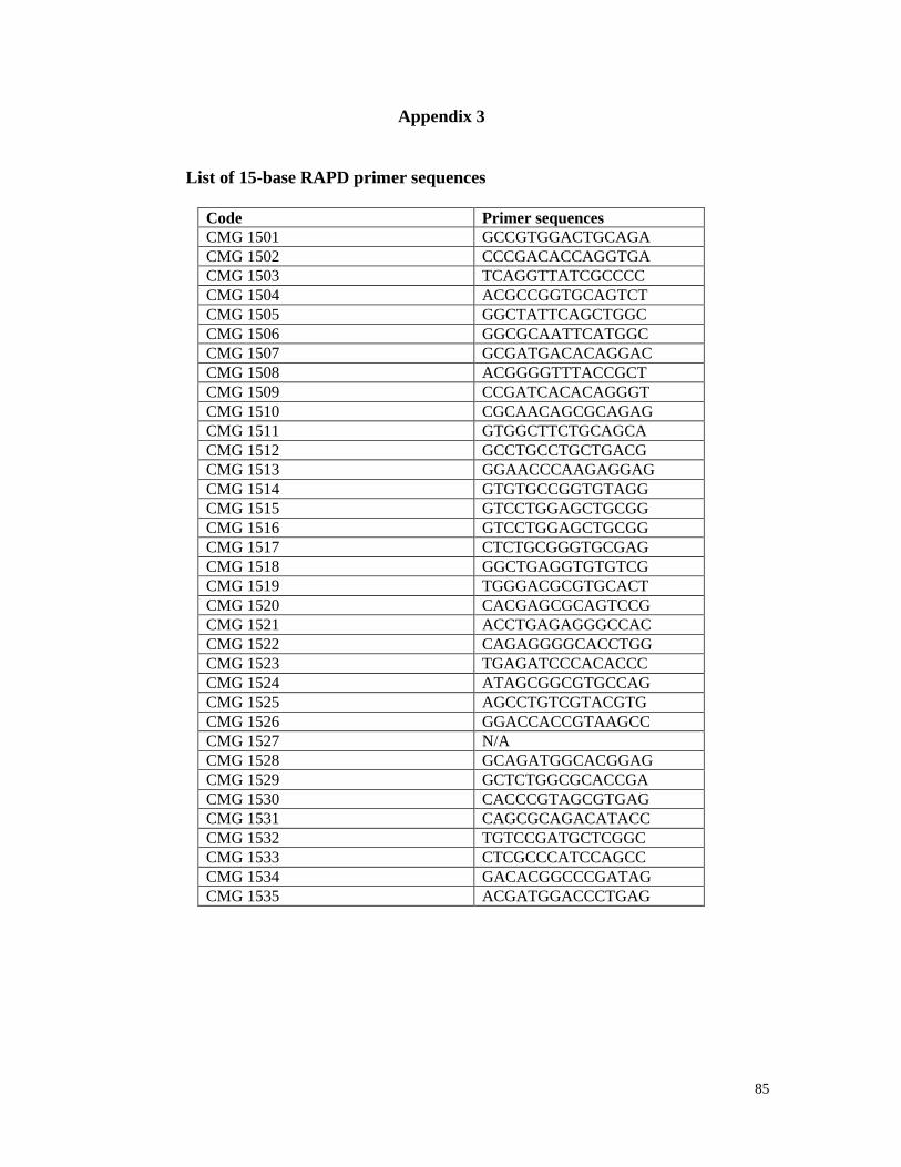
85

Appendix 3

List of 15-base RAPD primer sequences

Code Primer sequences

CMG 1501 GCCGTGGACTGCAGA

CMG 1502 CCCGACACCAGGTGA

CMG 1503 TCAGGTTATCGCCCC

CMG 1504 ACGCCGGTGCAGTCT

CMG 1505 GGCTATTCAGCTGGC

CMG 1506 GGCGCAATTCATGGC

CMG 1507 GCGATGACACAGGAC

CMG 1508 ACGGGGTTTACCGCT

CMG 1509 CCGATCACACAGGGT

CMG 1510 CGCAACAGCGCAGAG

CMG 1511 GTGGCTTCTGCAGCA

CMG 1512 GCCTGCCTGCTGACG

CMG 1513 GGAACCCAAGAGGAG

CMG 1514 GTGTGCCGGTGTAGG

CMG 1515 GTCCTGGAGCTGCGG

CMG 1516 GTCCTGGAGCTGCGG

CMG 1517 CTCTGCGGGTGCGAG

CMG 1518 GGCTGAGGTGTGTCG

CMG 1519 TGGGACGCGTGCACT

CMG 1520 CACGAGCGCAGTCCG

CMG 1521 ACCTGAGAGGGCCAC

CMG 1522 CAGAGGGGCACCTGG

CMG 1523 TGAGATCCCACACCC

CMG 1524 ATAGCGGCGTGCCAG

CMG 1525 AGCCTGTCGTACGTG

CMG 1526 GGACCACCGTAAGCC

CMG 1527 N/A

CMG 1528 GCAGATGGCACGGAG

CMG 1529 GCTCTGGCGCACCGA

CMG 1530 CACCCGTAGCGTGAG

CMG 1531 CAGCGCAGACATACC

CMG 1532 TGTCCGATGCTCGGC

CMG 1533 CTCGCCCATCCAGCC

CMG 1534 GACACGGCCCGATAG

CMG 1535 ACGATGGACCCTGAG

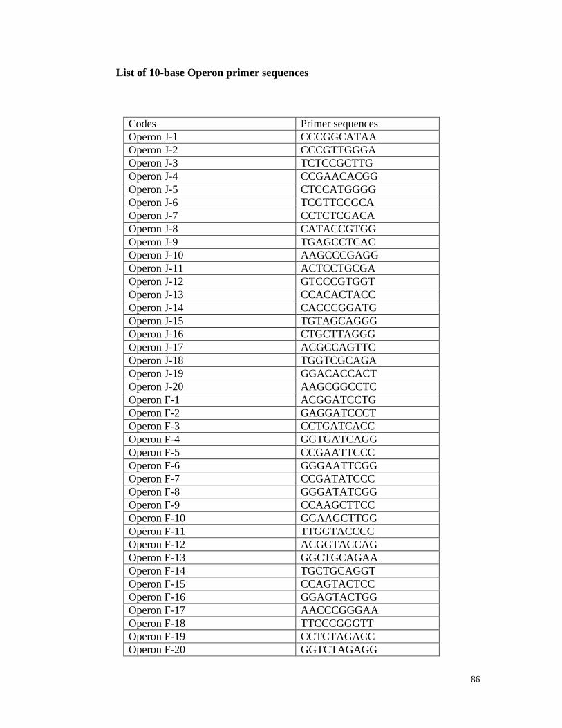
86

List of 10-base Operon primer sequences

Codes Primer sequences

Operon J-1 CCCGGCATAA

Operon J-2 CCCGTTGGGA

Operon J-3 TCTCCGCTTG

Operon J-4 CCGAACACGG

Operon J-5 CTCCATGGGG

Operon J-6 TCGTTCCGCA

Operon J-7 CCTCTCGACA

Operon J-8 CATACCGTGG

Operon J-9 TGAGCCTCAC

Operon J-10 AAGCCCGAGG

Operon J-11 ACTCCTGCGA

Operon J-12 GTCCCGTGGT

Operon J-13 CCACACTACC

Operon J-14 CACCCGGATG

Operon J-15 TGTAGCAGGG

Operon J-16 CTGCTTAGGG

Operon J-17 ACGCCAGTTC

Operon J-18 TGGTCGCAGA

Operon J-19 GGACACCACT

Operon J-20 AAGCGGCCTC

Operon F-1 ACGGATCCTG

Operon F-2 GAGGATCCCT

Operon F-3 CCTGATCACC

Operon F-4 GGTGATCAGG

Operon F-5 CCGAATTCCC

Operon F-6 GGGAATTCGG

Operon F-7 CCGATATCCC

Operon F-8 GGGATATCGG

Operon F-9 CCAAGCTTCC

Operon F-10 GGAAGCTTGG

Operon F-11 TTGGTACCCC

Operon F-12 ACGGTACCAG

Operon F-13 GGCTGCAGAA

Operon F-14 TGCTGCAGGT

Operon F-15 CCAGTACTCC

Operon F-16 GGAGTACTGG

Operon F-17 AACCCGGGAA

Operon F-18 TTCCCGGGTT

Operon F-19 CCTCTAGACC

Operon F-20 GGTCTAGAGG

87

Codes Primer sequences

Operon E-1 CCCAAGGTCC

Operon E-2 GGTGCGGGAA

Operon E-3 CCAGATGCAC

Operon E-4 GTGACATGCC

Operon E-5 TCAGGGAGGT

Operon E-6 AAGACCCCTC

Operon E-7 AGATGCAGCC

Operon E-8 TCACCACGGT

Operon E-9 CTTCACCCGA

Operon E-10 CACCAGGTGA

Operon E-11 GAGTCTCAGG

Operon E-12 TTATCGCCCC

Operon E-13 CCCGATTCGG

Operon E-14 TGCGGCTGAG

Operon E-15 ACGCACAACC