do an insider’s wealth and income matter in the decision ... · do an insider’s wealth and...

Do an Insider’s Wealth and Income Matter in the Decision to

Engage in Insider Trading?

Juha-Pekka KALLUNKI*

University of Oulu, Department of Accounting

P.O. Box 4600, FIN-90014 University of Oulu, Finland

[email protected]

Jenni MIKKONEN

University of Oulu, Department of Accounting


[email protected]

Henrik NILSSON

Stockholm School of Economics, Department of Accounting

P.O. Box 6501, SE-113 83 Stockholm, Sweden

[email protected]

Mikko PUHAKKA

University of Oulu, Department of Economics


[email protected]

May 21, 2017

*Corresponding author

The authors wish to thank Euroclear Sweden, Finansinspektionen, the Swedish Tax Authorities and the

Swedish Research Council for providing the requisite data. This study has been evaluated and approved by

the Regional Ethical Review Board in Umeå, Sweden (DNR 08:074 Ö and DNR I3-0449/2009). The

authors gratefully acknowledge financial support from the NASDAQ OMX Nordic Foundation,

Vetenskapsrådet, the Handelsbanken Research Foundation, the Finnish Savings Banks Group Research

Foundation, the Marcus Wallenberg Research Foundation, the Finnish Cultural Foundation and the

Academy of Finland [Project #243017121].

1

Do an Insider’s Wealth and Income Matter in the Decision to

Engage in Insider Trading?

Abstract

We develop a theoretical model for analyzing the role of an insider’s wealth and income level

in her decision to engage in informed insider trading. In our model, the risk-averse insider

maximizes her expected utility by trading off the financial gain against the costs of informed

insider trading, both of which comprise a fixed component and a variable component related to an

insider’s wealth and income level through the volume of insider trading. We empirically test the

predictions of our model using large archival data of all corporate insiders in listed firms in Sweden

and reported insider trades by these insiders. Consistent with the model, we find that insiders’

willingness to time their selling prior to stock price declines significantly decreases with the level

of their wealth and income. We also find that less wealthy insiders with lower risk aversion,

measured by their criminal behavior, are particularly prone to timing their selling to avoid

declining stock prices. These results remain similar after controlling for various insider- and firm-

specific determinants of insiders’ trading decisions.

JEL Classification: M41, G10, G30, K42

Keywords: Insider trading, Wealth, Income

1. Introduction

A body of literature shows that corporate insiders’ trades predict future abnormal returns,

suggesting that insiders generally exploit their information advantage about firm prospects to make

trading decisions (e.g., Seyhun, 1986; Lakonishok and Lee, 2001; Jeng, Metrick and Zeckhauser,

2003; Huddart et al., 2007; Cohen et al., 2012).1 However, the abnormal returns that insiders have

been reported to earn are, on average, surprisingly small to justify them engaging in informed

trading to begin with, given the potential costs involved. In particular, the general public and

regulatory authorities monitor insiders’ trading and impose costs on insiders when trading is

perceived to be opportunistic and self-serving. These costs comprise both the potential reputational

1 Corporate insiders’ trades refer to their trades on the stocks of their own firms which must be disclosed

to the regulatory authority and to the general public. In Sweden, this regulatory authority is the

Finansinspektionen (the Swedish Financial Supervisory Authority), and in the United States it is the U.S.

Securities and Exchange Commission (SEC). Informed insider trading refers to corporate insiders’ stock

purchases (sales) that they time before abnormal stock price increases (declines).

2

losses imposed by outside investors and the media and the potential legal sanctions taken by the

regulator (e.g., Seyhun, 1992; Gao et al., 2014; Dai et al., 2015). Thus, an important, yet largely

unsolved question is why insiders decide to engage in informed trading, given the small average

abnormal returns and the potential costs of such trading.

In this paper, we address this question by arguing that less wealthy insiders are more likely to

trade on private information, because their returns to such trading are large enough to compensate

for the potential costs involved, compared to wealthier insiders. We moreover argue that even the

less wealthy insiders refrain from informed trading, if the costs associated with being detected are

large enough and do not compensate for the returns that could be earned by trading. We begin by

proposing a model of an insider’s decision to engage in informed insider trading. In the model, the

risk-averse insider maximizes her expected utility by trading off between the financial gain and

costs of informed insider trading, both of which include a fixed component and a variable

component related to the insider’s wealth and income level through the volume of insider trading.2

We show that an increase in the insider’s wealth and income level will decrease her willingness to

trade on private information, as long as the trading is subject to a relatively low risk of legal

enforcement and therefore not likely to incur large fixed costs such as criminal fines or jail time

for the insider. The reason is that a less wealthy insider would be willing to accept a lower

probability that her informed trading will not be detected and punished by outsiders than a wealthy

insider. This effect is greater in magnitude when the variable costs of trading on private

information such as personal reputational damages and other costs related to the volume of insider

trading are larger and the insider has lower risk aversion.

We empirically test the predictions of our model using data from Sweden, where archival data

on individual wealth, income and many other demographic variables are available for all insiders

of listed firms. Our data set covers 3,388 corporate insiders from all Swedish listed firms and

14,672 reported insider trades by these insiders over the period from 2000 to 2008. Corporate

insider trading does not typically fall under the definition of legally material information and is

consequently associated with low risk of legal enforcement actions taken by the regulator,

including criminal fines, disgorgement of profits or even jail sentences (Seyhun, 1992, 1998).

2 Strictly speaking, an economic agent maximizes her expected utility obtained from consumption,

where the level of consumption is determined by her wealth and income levels as in the standard portfolio

theory. We include in our empirical analyses both an insider’s wealth and income.

3

However, insider trades considered to generate excessive personal gains may attract negative

investor and media attention, thereby damaging insiders’ reputational capital and also increasing

the likelihood of scrutiny by the regulator (Gao et al., 2014; Dai et al., 2015).

We find that the level of wealth and income varies substantially across the insiders in our

sample. When we divide insiders into three categories based on the level of their wealth and

income, we find that, on average, insiders in the low wealth and income category (‘less wealthy

insiders’) are considerably less wealthy than insiders in the medium and high (‘wealthy insiders’)

wealth and income categories. In particular, the average insider in the low wealth and income

category has a personal wealth of only $266,747, whereas the wealth owned by the average insider

in the medium (high) wealth and income category is as much as $6,895,621 ($12,374,131), a 26

(46) times difference. Similarly, insiders with a low level of wealth and income earn, on average,

only $72,294 per year, which is 2.5 (7) times less compared to insiders with a medium (high) level

of wealth and income. These differences suggest that the insider trading behavior could indeed

differ between insiders with different levels of wealth and income.

Consistent with our model, the empirical results of analyzing reported insider trades show that

insiders’ willingness to engage in informed insider selling significantly decreases with the level of

their wealth and income. Specifically, we find that less wealthy insiders are more likely to time

their selling prior to abnormal stock price declines than wealthy insiders. The size of less wealthy

insiders’ sales moreover increases with the magnitude of the future stock price decline. The mean

(median) buy-and-hold abnormal (market-adjusted) stock return over a one-month period

following a single insider sale transaction by less wealthy insiders is –1.70 percent (–2.44 percent),

which translates into an economically significant annualized return of –18.6 percent (–25.3

percent). In contrast, the mean and median abnormal returns following the sales by wealthy

insiders are not significantly negative.

We also find that, conditional on being less wealthy, insiders who are more risk-prone as

measured by their criminal convictions are more likely to time their selling to avoid stock price

declines, compared to non-convicted insiders. We do not observe similar selling behavior for

wealthy risk-prone insiders. These results continue to hold after controlling for other likely motives

for insiders to sell their stocks besides exploitation of private information, including insiders’

portfolio diversification objectives, liquidity needs, capital gain taxation considerations, contrarian

trading behavior, information asymmetry and other firm characteristics, and year and firm fixed

4

effects. These findings are consistent with less wealthy insiders valuing the financial gain from

informed insider selling more than the associated reputational and legal costs. The results also

suggest that wealthy insiders’ concerns with these potential costs outweigh their benefit from

selling on private information, and they therefore decide to time their selling more carefully.

Interestingly, we do not find the same contrasting patterns for insiders’ purchases, which they

time prior to stock price increases regardless of the level of their wealth and income or attitude

towards risk. The asymmetry of this finding is consistent with the argument made in prior research

that the reputational and legal risk associated with being detected for trading on private information

is significantly higher for insider sales compared to purchases (e.g., Cheng and Lo, 2006; Piotroski

and Roulstone, 2007; Brochet, 2010; Dai et al., 2015; Alldredge and Cicero, 2015).

We also examine the abnormal post-trade returns earned by insiders with different levels of

wealth and income by calculating the intercept from the CAPM and the Fama and French three-

factor and four-factor calendar-time portfolios. We confirm that, on average, less wealthy insiders

earn superior returns from trading in their firms’ shares after controlling for risk factors, compared

with wealthy insiders. The difference in the returns earned by less and more wealthy insiders is

also economically significant. For instance, the portfolio of less wealthy insiders’ sales (purchases)

yields a monthly return of –1.66 percent (1.68 percent) over the portfolio of wealthy insiders’ sales

(purchases), controlling for market risk, size, book-to-market and stock return momentum

characteristics of the traded stocks.

Our paper contributes to the limited literature on how insiders’ personal characteristics or

traits affect their insider trading behavior by shedding more light to the question of why some

insiders decide to engage in informed trading given the small average abnormal returns

documented in prior studies and the potential costs of trading (e.g., Kallunki et al. 2009; Gao et

al., 2014; Davidson et al., 2016; Hillier et al., 2015; Kallunki et al., 2016). The paper closest to

ours is Kallunki et al. (2009), who find that insiders’ portfolio diversification needs, tax

considerations and behavioral biases affect their trading decisions and that insiders who have

allocated a great proportion of their wealth to insider stock sell more before bad news. We expand

these papers, especially Kallunki et al. (2009), in the following ways. First, to the best of our

knowledge, this is the first paper that presents a theoretical model of how the level of an insider’s

wealth and income affects her trade-off between the financial benefit and costs of informed insider

trading, and consequently, leads to differential trading behavior by less and more wealthy insiders.

5

Second, while Kallunki et al. (2009) consider an insider’s portfolio diversification needs

measured as the proportion of her total wealth allocated to insider stock as an incentive for trading

on private information, they do not explore whether the level of an insider’s wealth and income

affects how she considers the potential financial gain and associated cost from engaging in

informed insider trading. Analyzing an insider’s expected utility from her wealth and income

allows us to address the question of why insiders engage in informed trading, given the small

abnormal insider returns documented in the literature. Consistent with this view, our empirical

results show that the diversification-driven insider selling reported by Kallunki et al. (2009) and

less wealthy insiders’ selling are distinct behavior by insiders. Third, we examine how the insider’s

risk aversion, measured by their criminal behavior, affects her willingness to engage in informed

trading, given the level of her wealth and income.

Finally, this paper contributes to the recent literature that focuses on the role of individuals

and their personal characteristics or traits, as opposed to firm- or industry-level factors, in shaping

corporate behavior and outcomes (e.g., Bertrand and Schoar, 2003; Kaplan, Klebanov, and

Sorensen, 2012; Malmendier and Tate, 2008; Cronqvist, Makhija, and Yonker, 2012). We show

that corporate insiders’ personal characteristics play a role not only in shaping corporate decisions,

but also in their decisions related to stocks of their own firm. The rest of the paper is organized as

follows. In Section 2, we describe our theoretical model for an insider’s decision of whether to

engage in informed insider trading and report numerical simulations of the model. Section 3

describes our data and empirical methodology. Section 4 presents the empirical results. Finally,

we provide concluding remarks in Section 5.

2. Model

In this section, we present a model that forms the basis of the empirical analysis. Our model

follows the tradition of the economics of crime going back to the seminal work by Becker (1968).

Consider an informed insider who contemplates engaging in informed insider trading. The

insider’s utility ultimately depends on the level of her consumption, which in turn depends on the

level of her wealth and income, denoted by W.3 We assume that the utility function u(W) is strictly

increasing and strictly concave:

3 Since we have a one-period model, all of the income and wealth end up in consumption.

6

(1) U = u(W) with u'(W) > 0 and u''(W) < 0.

In addition, we assume the following Inada conditions:

(2)

)('0

limWu

Wand 0)('

lim

Wu

W.

All of the standard utility functions fulfil these conditions, which guarantees that the optimal

solution is not in the corners. Since the utility function is strictly concave, Jensen’s inequality

implies that u(EW) > Eu(W), where E is the expectations operator.

When deciding whether to engage in informed insider trading, the insider maximizes her

expected utility by trading off the financial gain against the costs of such trading. The insider’s

financial gain from her trade is denoted by ηV, where η is the expected percentage change in the

stock price given the insider’s private information, and V is the (dollar) value of the shares traded,

i.e., the number of shares traded times the stock price. An insider has a budget constraint in her

trading decisions, that is, there is an upper limit for how many shares she can buy or sell in an

insider trade, the limit being determined by her wealth and income level.4 There is also a minimum

number of shares Vmin (> 0) that the insider must trade to cover the monetary and non-monetary

transaction costs.5 The value of an insider trade can therefore be defined as V = Vmin + θW, where

θ (0 ≤ θ < 1) is the fraction of the insider’s wealth and income level. The insider’s financial gain

can now be rewritten as η(Vmin + θW) = ηVmin + ηθW, where the term ηVmin represents the fixed

gain component and the term ηθW represents the variable gain component. Note also that, holding

θ fixed, the insider’s financial gain increases with the level of her wealth and income, W.

As for the costs of insider trading, classical theoretical settings with incomplete contracts and

informational asymmetries (e.g., Klein and Leffler, 1981; Kreps and Wilson, 1982; Shapiro, 1983)

suggest that reputation serves as an informal enforcement mechanism against opportunistic

corporate behavior, such as informed insider trading.6 Reputational concerns play an important

4 We assume that an insider does not sell short insider stocks and does not borrow money for insider

purchases. 5 Monetary and non-monetary transaction costs include, for instance, transaction fees, the costs of

reporting the transaction to the regulator, the costs of acquiring possible pre-approval for the transaction

from the company, and other transaction costs that the insider incurs when and if she decides to trade. 6 Empirical evidence supports the role of reputation in deterring and disciplining corporate misconduct

(see Macleod 2007 for a review). For example, Atanasov et al. (2012) show that reputational capital

disciplines and deters opportunistic behavior by venture capitalists. According to Gao et al. (2014),

executives in firms with a socially responsible image are more likely to refrain from informed trading,

especially when their personal reputation is more closely tied to the firms’ reputation or when they have

higher stock ownership. Dai et al. (2015) moreover show that dissemination of SEC insider trading filings

7

role in insiders’ trading decisions because insiders are required to publicly disclose their trading

activities. In particular, opportunistic insider trades are likely to capture negative investor and

media attention, thereby damaging insiders’ reputational capital and potentially increasing the

probability of regulatory scrutiny.7 Moreover, since insider trading is regulated by the legislation,

the insider’s trading on material private information could be subject to legal sanctions imposed

by the regulator including criminal fines, disgorgement of trading gains or even jail time.

Therefore, the costs of insider trading comprise both the potential reputational losses imposed

by outside investors and the media and the potential legal sanctions taken by the regulator (e.g.,

Seyhun, 1992; Gao et al., 2014; Dai et al., 2015).

Similarly to Seyhun (1992) and Acharya and Johnson (2010), we assume that there are both

fixed and variable costs of informed insider trading. These costs are denoted by d + φλW, where d

reflects the fixed costs of informed trading such as criminal fines and jail sentences and the term

φλW (λW = V and 0 < λ ≤ 1) describes the variable costs of informed trading, including

disgorgement of trading gains and other costs that are related to the insider trading volume and

hence to the magnitude of the profits gained or the losses avoided. For example, the degree of

negative publicity resulting from opportunistic trading behavior and thereby the damage to the

insider’s reputational capital and labor market prospects are likely to increase in the private

financial gain that the insider receives from her trading.

Finally, let p (1 – p) denote the probability that the costs of informed trading will not be (will

be) imposed on the insider by outsiders, i.e., outside investors, media members or the regulator.

Consequently, the insider’s expected utility from her informed trade is defined as

(3) EU = pu(W + ηM + ηθW) + (1 – p)u[W – (d + φλW)].

For notational simplicity, we write ηVmin, ηθ, and φλ as a, r, and c respectively. Hence, the

insider’s expected utility can now be rewritten as

(4) EU = pu[(1 + r)W + a] + (1 – p)u[(1– c)W – d].

by the media restricts insider trading profits because insiders are concerned about the adverse impact of

informed trading on their reputational capital and personal wealth. Karpoff (2011) notes that opportunism

against business counterparties such as investors typically leads to reputational losses that are much larger

than any legal penalties. 7 Opportunistic insider trades do not, however, necessarily trigger formal enforcement actions by the

regulator (Cohen et al., 2012; Dai et al., 2015).

8

In order for the maximization problem to be reasonable, we need the restriction that the final

wealth and income level (i.e., consumption) is positive, i.e. )1/( cdW . Note that Jensen’s

inequality entails:

(5) u(p[(1+r)W + a] + (1 – p)[(1– c)W – d]) > pu[(1 + r)W + a] + (1 – p)u[(1– c)W – d].

This implies that the necessary condition for the insider to engage in informed insider trading is

that the expected net gain from that activity must be positive, i.e.,

(6) p(rW + a) – (1 – p)(cW + d) > 0.

Note that Jensen’s inequality implies u(W) > Eu(W), if the expected net gain is zero. The insider

decides to engage in informed trade only if her expected utility following the trade is greater than

her utility if she does not trade:

(7) pu[(1 + r)W + a] + (1 – p)u[(1– c)W – d] > u(W).

Next, we assume that the utility function is of the constant relative risk aversion (CRRA) type,

i.e.,

(8)

1)(

1WWu with σ > 0 and σ ≠ 1,

where σ is the Arrow-Pratt measure of the relative risk aversion. If σ = 1, the utility function is

logarithmic. Our results below hold for all of the CRRA functions, including the logarithmic

function. A CRRA function is general and allows us to perform numerical illustrations.

To understand the conditions under which the insider decides to engage in informed insider

trading, we explore the combinations of the probability that the costs will not be imposed by

outsiders (p) and the level of the insider’s wealth and income (W) such that she is indifferent

between engaging and not engaging in informed trading. An indifferent insider decides not to

engage in informed trading. A lower (higher) probability for indifference means that the insider,

in deciding whether to engage in informed trading, accepts (requires) a lower (higher) probability

that such trading remains undetected and unpunished by outsiders. Hence, a lower (higher)

probability corresponds to the insider being more (less) willing to trade on the basis of private

information. The indifference condition is Eq. (7) written as an equality. Expressing the probability

p from the indifference relation as a function of W gives:

(9i)

11

11

)1()1(

)1(

dWcWra

dWcWp , when σ < 1 and

9

(9ii) 11

11

)1(

1

)1(

1

1

)1(

1

aWrdWc

WdWcp , when σ > 1.

We denote the indifference relations (9i) and (9ii) as ),;,;( dcarWzp , and characterize the

properties of this function in the following Propositions 1 and 2. We also analyze how changing

the magnitude of the fixed and the variable costs of informed insider trading influences the

insider’s decision whether to engage in insider trading, given the level of her wealth and income.

The proofs of the propositions are in Appendix A.

Proposition 1. The function ),;,;( dcarWz is an increasing function of the level of an insider’s

wealth and income, i.e., 0),;,;( dcarWzW , if the fixed costs are small relative to her wealth and

income, i.e., if Wd / is relatively small. Furthermore, the following properties hold:

0),;,;( dcarWzc and 0),;,;( dcarWzd .

Proposition 2. If Wd / is relatively small and σ > 1, the slope of the indifference curve with respect

to the level of an insider’s wealth and income gets steeper (flatter), if the variable costs (c)

increase (decrease). If σ < 1, the same result holds for a sufficiently small a, r, and c.

Proposition 1 says that a decrease in the level of an insider’s wealth and income increases her

willingness to engage in informed insider trading, as long as the fixed costs of such trading are

small relative to the insider’s wealth and income level. The reason is that a less wealthy insider

would be willing to accept a lower probability that her informed trading will not be detected and

punished by outsiders than a wealthy insider. Proposition 2 says that an increase (decrease) in the

variable costs of informed trading increases (reduces) the relation between the level of the insider’s

wealth and income and her willingness to engage in informed trading. Finally, the result in

Proposition 1 that 0),;,;( dcarWzc and 0),;,;( dcarWzd means that an increase in the fixed

or variable costs of informed trading will lead to a decline in the insider’s willingness to engage in

informed trading regardless of the level of her wealth and income. This is because the insider

10

requires a higher probability that her informed trading will not be detected (and punished) by

outsiders.

We illustrate the results in Propositions 1 and 2 numerically in Fig. 1, where we construct

three scenarios for an insider’s decision whether or not to engage in informed trading, given the

magnitude of the fixed and variable costs associated with such trading.8 In the first scenario, an

insider’s informed trading is subject to a low risk of legal enforcement and is thus not likely to

incur any fixed costs for the insider (d = 0), and also reputational damage and other variable costs

related to the magnitude of insider trading are small (c = 0.01). In the second scenario, an insider’s

informed trading still involves a low risk of legal enforcement (d = 0), but includes larger

reputational and other variable costs (c = 0.06) than in the first scenario. In the third scenario, an

insider’s informed trading is subject to a high risk of legal enforcement and thus likely to incur

large fixed costs (d = 1.0) and variable costs (c = 0.09) for the insider. In all these scenarios, we

set a = 0.5 and r = 0.05.

Fig. 1 depicts the probability p that makes the insider indifferent between trading and not

trading for varying levels of her wealth and income (W) in each of the three scenarios. As shown

in Fig. 1, the indifference probability p increases from the first to the third scenario for all levels

of wealth and income. In other words, an increase in the fixed or variable costs of informed trading

leads to a decline in the insider’s willingness to engage in such trading regardless of the level of

her wealth and income (Proposition 1). Fig. 1 also shows that the indifference curve increases with

the level of the insider’s wealth and income in the first and second scenarios, where the insider’s

informed trading is subject to a low legal risk and therefore likely not to involve any fixed costs

such as criminal penalties or jail time (Proposition 1).

The indifference curve is moreover steeper in the second than in the first scenario, indicating

that the insider’s wealth and income level has a greater impact on her willingness to engage in

informed trading when the variable costs are larger and has only a minor impact when the variable

costs are small (Proposition 2). Contrary to the first and second scenarios, the indifference curve

decreases with the increasing level of an insider’s wealth and income in the third scenario, where

8 We allow the level of the insider’s wealth and income, W, to range from 0.25 to 8.0. In Fig. 1, an

insider’s relative risk aversion coefficient, σ, is equal to 5.0, and in Fig. 2, σ is equal to 5.0 or 0.5. Note that

in order for the expected utility maximization problem to be reasonable, the insider’s final wealth and

income level must be positive, i.e. W > d / (1 – c). In addition, a necessary condition defined in Eq. (6)

holds in all numerical analyses.

11

informed trading is subject to a high risk of legal enforcement and thus likely to incur large fixed

and variable costs for the insider. The figure moreover shows that, in the third scenario, the

probability for indifference does not exist for very low levels of wealth and income.9 In other

words, when the legal risk of informed insider trading is high, it is not reasonable for an insider

with a very low level of wealth and income to even consider engaging in such trading.

(Insert Fig. 1 about here)

Finally, we examine numerically how the insider’s risk aversion affects her willingness to

engage in informed trading, given the level of her wealth and income, and the fixed and variable

costs. In particular, Fig. 2 plots the difference in the indifference probability between the insider

with high risk aversion (σ = 5.0) and the insider with low risk aversion (σ = 0.5) for varying levels

of wealth and income for each of the three scenarios described above. The figure illustrates that

the indifference probability is always higher for higher risk aversion, meaning that the insider is

less willing to engage in informed trading when she is more risk averse. This effect becomes

stronger as the costs of such trading increase. However, risk aversion has less impact on the

insider’s willingness to trade on private information when the insider is wealthy than when she is

less wealthy, irrespective of the amount of the costs.


3. Data and empirical methodology

3.1. Data sources

We use comprehensive archival data on Swedish insiders obtained from various nationwide

official databases maintained by Swedish tax, regulatory, and police authorities. All these data sets

are in electronic form, and we use individuals’ unique social security codes to merge different

databases. Our sample period is from 1 January 2000 through to 31 December 2008.10 The final

9 This is because the condition that W > d / (1 – c) must hold in order for the insider’s expected utility

maximization problem to be reasonable to begin with. 10 The Swedish Tax Agency has not collected the data on taxpayers’ personal wealth after 2007, which

limits our sample period. Although comprehensive archival data on insiders’ wealth and income is not

publicly available in many countries, such data could be accessed by regulatory authorities screening insider

12

sample includes 3,388 insiders, 393 firms and 14,672 insider trades, consisting of 5,589 insider

sales and 9,083 insider purchases.

Our data on daily insider transactions is obtained from the Finansinspektionen, which is the

corresponding regulatory authority to the U.S. SEC. This data set includes an insider’s name, a

social security code, the name of the firm traded, the number of shares traded and the day on which

the transaction was made. Following the literature on insider trading, we focus on open market

purchases and sales by corporate insiders and exclude non-open market transactions, such as

option exercises, transactions related to bonuses, pension and other benefit program transactions,

and gifts. In the case of multiple insider transactions on the same day for a given insider and her

insider firm, we net all these transactions.11

The insider trading legislation in Sweden is in accordance with European Union Directives on

the Regulation of Insider Trading (EEC Directive 89/592) and on Insider Dealing and Market

Manipulation (Directive 2003/6/EC). The Swedish insider legislation is of high quality and quite

similar to that of the USA (Beny, 2005). The main differences are as follows. First, while illegal

insider trading is both a criminal and a civil offence in the USA, it is only a criminal offence in

Sweden. Hence, unlike the SEC in the USA, the Finansinspektionen in Sweden lacks a civil

enforcement authority in illegal insider trading. Second, the maximum penalty for trading illegally

on insider information in the USA is 10 years of imprisonment, compared with the maximum of 4

years in Sweden.

In addition to formal insider trading laws, country-level corporate culture and governance may

influence how acceptable trading on inside information is viewed in corporate practice and by the

public and consequently, the likelihood and magnitude of reputational damage resulting from

profitable insider trading as perceived by insiders. As for the level of corporate governance,

Aggarwal et al. (2009) find that Sweden places among the top ten countries, not far from the USA.

Denis and Xu (2013) moreover report that, like US executives, Swedish executives consider

insider trading not to be a common practice in the domestic market. In sum, although there are

trades. Moreover, previous studies on U.S. insiders have used publicly available, although less precise,

proxies for the level of their wealth and income including home values (Ahern, 2017), the value of shares

owned in the firm (Gao et al., 2014) and annual compensation (Roulstone, 2003). Hence, we believe that

our results based on comprehensive archival data point to insiders’ trading behavior that could be traced

even with less precise data on insiders’ wealth and income. 11 We also exclude very small trades (size of trade < SEK 10,000) from our analyses. SEK 1 is equal to

USD 0.12.

13

some differences in insider trading legislation, its enforcement, corporate cultures and the level of

corporate governance between Sweden and the USA, previous research suggests that these

differences are small. Appendix B briefly discusses the details of the insider trading legislation in

Sweden and compares it with that of the USA.

We obtain the data on insiders’ personal wealth, including the values of real estate, mutual

funds, bank holdings, investments in debt securities and taxable labor income from the Swedish

tax authorities (Skatteverket). These data are reported on an annual basis and are public information

in Sweden. We obtain the data on insiders’ insider and outsider stockholdings from the Nordic

Central Securities Depository Group (NCSD). The NCSD maintains an electronic database on the

ownership of all Swedish stocks, in which the data are recorded at six-month intervals. From these

data, we are also able to identify an insider’s year of birth, gender and a position as an insider.

The data on insiders’ criminal convictions are from the Swedish National Council for Crime

Prevention (Brå). This data set is a record of all individuals who have been found guilty by a court

of law or received summary punishment from prosecutors since 1974. The data set does not include

minor offences such as speeding, parking and violations of local bylaws for which the punishment

is an on-the-spot fine. Following previous studies (e.g., Korsell, 2001; Amir et al., 2014), we also

include data on individuals who have been under investigation for serious crimes to reduce the

selection bias from focusing only on individuals who are actually convicted. The data on suspected

criminal actions by corporate insiders are obtained from the Swedish National Police Board and

are a record of all Swedish citizens who have been under investigation for serious crimes since

1991. Finally, we merge our insider transaction data with firm-level data from Thomson

Datastream, including daily stock prices, market capitalizations and annual accounting data.

3.2. Sample construction

We model insiders’ decisions to trade their insider stocks using the matched-pair research

design commonly used in previous studies exploring insiders’ trading behaviour (e.g., Noe, 1999;

Kallunki et al., 2009). We begin by identifying all days when an insider i trades on her insider

stock j from our data on daily insider trades. For each insider i and stock j, we then construct a

time series of all trading days over the sample period from 1 January 2000 through 31 December

2008. These time series include trading days when there is insider trading and days when there is

no insider trading. For each day when there is insider selling (buying) for a given firm, we

14

randomly choose a day without insider selling (buying) from all trading days over the sample

period for that firm. The resulting sample has an equal number of 5,589 (9,083) days with insider

selling (buying) and 5,589 (9,083) days without insider selling (buying).

3.3. Measurement of variables

3.3.1. Dependent variables

We construct the following two variables to measure insiders’ decisions to engage in informed

insider trading. First, we measure insiders’ decisions to sell (buy) their insider stocks by a dummy

variable TRADEijt, which equals one if insider i sells (buys) her insider stocks of firm j on day t,

and zero otherwise. Second, we measure insiders’ decisions regarding the magnitude of their sales

(buys) by SIZEijt, which is the natural logarithm of the market value of the shares sold if insider i

sells (buys) insider stocks of firm j on day t, and zero otherwise. In untabulated analyses, we obtain

similar results using the percentage of the market value of shares sold (bought) of the value of

insider holdings (SIZE_HOLDijt) or the percentage of the market value of shares traded of the value

of total personal wealth (SIZE_WEALTHijt).

3.3.2. Independent variables

3.3.2.1. Level of wealth and income

We construct a measure of the level of an insider’s wealth and income using the following

procedure. First, we assign all observations in our matched-pair sample of the 11,178 (18,166)

observations used for analyzing insider selling (buying) into two equal-sized portfolios based on

the level of an insider’s wealth at the end of the previous fiscal year, i.e., low-wealth and high-

wealth portfolios. Accordingly, we assign all observations in the matched-pair sample into two

equal-sized portfolios based on the level of insiders’ annual income from the previous year, i.e.,

low-income and high-income portfolios. We then assign all observations that belong to the

portfolios of both low-wealth and low-income into the category ‘Low’. In a similar way, we assign

all observations that belong to the portfolios of both high-wealth and high-income into the category

‘High’. Finally, the remaining observations, i.e., those that belong to the portfolios of high-wealth

and low-income or to those of low-wealth and high-income, we assign into the category ‘Medium’.

Based on the categories ‘Low’, ‘Medium’ and ‘High’, we construct dummy variables LOWit,

HIGHit and MEDit to identify insiders with different levels of wealth and income. Specifically,

15

LOWit is a dummy variable equal to one if an observation in our match-paired sample belongs to

the category ‘Low’, and zero otherwise; HIGHit is a dummy variable equal to one if an observation

belongs to the category ‘High’, and zero otherwise; and MEDit is a dummy variable equal to one

if an observation belongs to the category ‘Medium’, and zero otherwise. In Section 4.4.2., we use

an alternative way for grouping insiders based on the level of their wealth and income and find

similar results.

3.3.2.2. Stock return

The variable BHARjt is the buy-and-hold abnormal (market-adjusted) stock return for a one-

month period following day t for firm j. A more negative (more positive) abnormal stock return

following an insider sale (purchase) indicates exploitation of private information by the insider

who made the trade. We choose a one-month return horizon because timing insider trades shortly

before large abnormal changes in the stock price is likely to be subject to greater public and

regulatory scrutiny and therefore involves higher risk of personal reputation damage or even legal

sanctions for the insider. We have also used a three-month and a six-month horizon for future

returns and obtained essentially similar results.12 These results are not tabulated for the sake of

brevity.

3.3.2.3. Criminal convictions

We use an insider’s criminal behavior to measure her attitude towards risk. Specifically, broad

literature shows that criminal behavior is an indicator of an individual’s higher propensity to take

risks (e.g., Ehrlich, 1973; Junger et al., 2001; Garoupa, 2003). Economic theory of crime suggests

that the decision to engage in criminal activity is rational behavior under uncertainty, and that

individuals engage in criminal acts if the expected utility from those acts is greater than the utility

received from non-criminal behavior (Becker, 1968; Ehrlich, 1973). Ehrlich (1973) shows that a

risk-neutral individual spends more time on illegal activities than a risk-averse person, and a risk-

loving person spends more time on such activities than both of these other persons. In addition,

the behavioral research on crime links criminal behavior to individuals’ personal preferences like

12 The only exception is that when we use a six-month horizon for future returns, the estimated parameter

for the three-way interaction variable LOWit×RISK_TAKERi×BHARjt is not significantly negative in Tobit

regression (p=0.229).

16

overconfidence (e.g., Iversen and Rundmo, 2002; Garoupa, 2003). This literature suggests that

many criminals are overconfident risk-takers who have overly optimistic beliefs about the

uncertain outcomes of their actions and seem to ignore or not think about the likelihood of

punishment, which could then reduce its deterrent effect (Garoupa, 2003).

Overall, the literature discussed above suggests that convicted insiders are likely to have lower

risk aversion than their non-convicted peers. In addition, being overly confident may make

convicted insiders underestimate the probability that their informed insider trades will be detected

(and punished) by outsiders (Bénabou and Tirole, 2002; Van den Steen, 2004; Brunnermeier and

Parker, 2005). To measure an insider’s attitude towards risk, we construct a dummy variable

RISK_TAKERi, which equals one if insider i has been found guilty of a crime in a court of law,

received summary punishments by prosecutors or been suspected of a serious crime, and otherwise

zero. We have also re-estimated all our regressions by using the natural logarithm of one plus the

number of times insider i has been found guilty of a crime in a court of law, received summary

punishments by prosecutors or been suspected of a serious crime. These untabulated results are

similar to those based on the dummy variable.

3.3.2.4. Control variables

In our regressions, we include insider- and firm-level control variables that are likely to

influence insiders’ trading decisions. We control for insiders’ gender (GENDERi) because previous

studies report that male and female insiders trade differently (e.g., Barber and Odean, 2001;

Kallunki et al., 2009). Following Jin and Kothari (2008), we also include control variables for

insiders’ age (AGEi) and tenure to account for their entrenchment and career concerns

(TENUREijt). We also control for the number of firms in which she is an insider (NUMINSijt) and

her position as an insider in her insider firm with two dummy variables for those insiders who are

employed either as the CEO (CEOijt) or as another executive (EXECijt).

To control for insider trading due to portfolio re-balancing (Ke et al., 2003; Huddart and Ke,

2007; Kallunki et al., 2009), we include in the regressions the proportion of insiders’ total wealth

allocated to their insider stock (PROP_WEALTHijt).13 In addition, we control for insiders’ tendency

13 We replicated all our analyses by using the difference of the proportion of an insider’s total wealth

allocated to her insider stock and the time-series mean of this proportion calculated for each insider over

the sample period of nine years as in Kallunki et al. (2009), and find similar results.

17

to follow a contrarian trading strategy (Rozeff and Zaman, 1998; Piotroski and Roulstone, 2005)

with the variables MOMENTUMjt and PBjt. We also control for the degree of information

asymmetry with the firm’s idiosyncratic return volatility (IVOLjt). In the insider-selling models,

we control for insider trading for liquidity reasons with the variable measuring their cash and other

liquid assets of the wealth (LIQUIDITYit) and for insiders’ tendency to sell their losing stocks at

the end of the year for capital taxation purposes (DECLOSSjt). We also control for the potential

effect of firm profitability (ROAjt) and firm size (MVjt). We include two dummy variables PREjt

and POSTjt to control for insiders’ differential trading activity before and after earnings

announcements (Huddart et al., 2007; Kallunki et al., 2009). We further control for the short-term

stock returns around the day on which an insider trades (LAG_kjt, RETjt and LEAD_kj).

Finally, we use firm-fixed effects to control for the effects of possible omitted time-invariant,

firm-specific factors of insider trading (FIRM_sj) and also include eight yearly dummy variables

for the years 2000-2007 to control for time-specific effects (YEAR_y).

3.4. Summary statistics

Table 1 provides summary statistics on insiders’ wealth and income (Panel A), insider trading

behavior (Panel B) and criminal behavior (Panel C) of all 3,388 insiders in our sample. The average

(median) insider has a personal wealth of SEK 49,636,500 (SEK 4,666,500) and an annual salary

income of SEK 1,826,900 (SEK 1,063,600).14 Moreover, the level of an insider’s wealth and

income varies considerably across insiders in our sample. Panel B of Table 1 shows that the

average insider made 3.18 (3.53) sale (buy) trades during the sample period of nine years.

Consistent with the previous literature (e.g., Lakonishok and Lee, 2001), insiders’ sales are greater

than their purchases. The average insider sold (bought) 28.42 percent (22.07 percent) of her insider

holdings and 14.70 percent (7.52 percent) of her total wealth. There is also great variation in these

percentage figures across insiders. Panel B of Table 1 also reports the buy-and-hold abnormal

(market-adjusted) returns that insiders earn from their sales and purchases, measured over a one-

month period following an insider trade. Consistent with prior research (e.g., Seyhun, 1986;

Lakonishok and Lee, 2001; Jagolinzer et al., 2011; Alldredge and Cicero, 2014), the mean and

median abnormal returns following insider purchases are larger than those following insider sales.

Panel C of Table 1 shows that 899 (26.5 percent) out of all 3,388 insiders in the sample have been

14 SEK 1 was equal to USD 0.12 during our sample period.

18

convicted or suspected of one or more crimes. While this percentage figure may seem high to

many, it is similar to that of the whole Swedish population (Svensson, 2000).

(Insert Table 1 about here)

Table 2 reports summary statistics for insiders’ selling (Panel A) and buying (Panel B) activity,

by the magnitude of the one-month buy-and-hold abnormal (market-adjusted) return following an

insider trade. As shown in Panel A of Table 2, the number of insider sales monotonically decreases

with the magnitude of the future stock price decline, indicating that insiders tend to refrain from

selling prior to declining stock prices. When insiders do, however, sell before stock price declines,

they realize economically significant gains by avoiding losses. For instance, the average insider

who sells before a stock price decline between 20 and 25 percent (more than 40 percent) avoids a

loss of SEK 165,680 (SEK 204,440) over a one-month period, which represents 2.92 percent (6.90

percent) of her total wealth.15

Interestingly, Panel A of Table 2 also shows that less wealthy insiders (those in the wealth and

income category ‘Low’) clearly sell more frequently before larger stock price declines than

wealthy insiders (those in the wealth and income category ‘High’). In particular, the proportion of

insider sales made by less wealthy insiders increases with the magnitude of the future stock price

decline, whereas that of the sales made by wealthy insiders decreases. To illustrate, roughly 29

percent (38 percent) of all insider sales preceding stock price declines of 5 percent or less are

conducted by insiders in the low (high) wealth and income category, whereas low (high)

wealth/income insiders constitute 64 percent (18 percent) of all the sales made before stock price

declines of more than 40 percent.

Regarding insiders’ purchasing activity, Panel B of Table 2 shows, similarly to insider sales,

that the number of insider purchases decreases with the magnitude of the future stock price

increase, with the exception of future returns more than 40 percent. Insiders also earn economically

significant gains for their purchases that are made before stock price increases. For example, the

mean gain from a purchase made before a stock price increase between 20 and 25 percent (more

15 In each abnormal return category, the mean loss avoided as percent of an insider’s total wealth is of

similar magnitude across the three wealth and income categories ‘Low’, ‘Medium’ and ‘High’ (not

tabulated).

19

than 40 percent) is SEK 152,470 (SEK 190,200), which equals 1.65 percent (4.22 percent) of an

insider’s total wealth. Finally, Panel B of Table 2 shows that the proportion of insider purchases

made by insiders in the low (high) wealth and income category generally increases (decreases)

with the future stock price increase. However, this phenomenon is not as strong as it was for insider

selling in Panel A.


Finally, Table 3 provides descriptive statistics for the selected independent variables based on

our matched-pair sample of 11,178 and 18,166 days with and without insider selling (Panel A) and

buying (Panel B).


4. Empirical results

4.1. Univariate analysis

Table 4 reports the results of the univariate analysis to explore whether the level of an insider’s

wealth and income affects her decision to engage in informed insider trading, that is, to time her

selling (buying) before abnormal stock price declines (increases). Specifically, we test whether the

mean and median future one-month abnormal returns (BHARjt) are significantly different between

the days with and without insider trading in our matched-pair sample. We conduct this analysis for

all insiders as well as for insiders in our three wealth and income categories (‘Low’, ‘Medium’ and

‘High’). Fig. 3 moreover plots the mean abnormal return over a one-month period following days

with insider selling and buying in the three wealth and income categories. The abnormal returns

following insider purchases are multiplied by –1 to make the figure comparable to Fig. 1. Thus,

higher abnormal returns indicate that insiders are more cautious in making their trading decisions.

Table 4 shows that there is substantial variation in the level of insiders’ wealth and income

across the three categories, with insiders in the low wealth and income category (the category

‘Low’) being considerably less wealthy than those in the other two categories (‘Medium’ and

20

‘High’).16 In particular, the average insider in the low wealth and income category has a personal

wealth of only $266,747, which is 26 and 46 times less than the personal wealth of the average

insider in the medium and high wealth and income categories, respectively. Similarly, the average

insider in the category ‘Low’ earns only $72,294 per year, which is 2.5 and 7 times less than that

earned by the average insider in the categories ‘Medium’ and ‘High’, respectively.

The univariate results for insider selling presented in Panel A of Table 4 show that the mean

(median) future abnormal return is significantly lower on days when insiders sell than on days

when they do not sell, suggesting that the average insider times her selling successfully. However,

only the insiders in the low wealth and income category (‘Low’) time their stock sales before price

declines, whereas the insiders in the other two wealth and income categories (‘Medium’ and

‘High’) do not. The mean (median) abnormal return following insider sales by insiders in the low

wealth and income category is –1.70 percent (–2.44 percent), which is both statistically and

economically significant. These returns translate into annualized returns of –18.6 percent (mean)

and –25.3 percent (median). These are economically significant numbers given that they result

from one single transaction. In contrast, the mean (median) abnormal return following sales by

insiders either in the medium or high wealth and income category is not significantly negative.

This can also be seen in Fig. 3.

The above analysis provides evidence consistent with less wealthy insiders, on average,

considering the expected utility gain of avoiding financial losses due to a decline in stock price to

outweigh the disutility due to costs of informed selling. The results also indicate that wealthy

insiders, on average, forgo the potential financial gain of informed insider selling to avoid the costs

associated with the more profitable insider trading. Our finding that less wealthy insiders are more

willing to gain from insider selling than wealthy insiders is consistent with our model’s prediction

that insiders’ willingness to trade on private information decreases with the level of their wealth

and income, as long as such trading is likely subject to a low risk of legal enforcement and hence

likely not to incur fixed costs (criminal fines, jail time) for the insider (Proposition 1). It is also

consistent with previous research suggesting that the vast majority of corporate insiders’ trades do

16 The mean and median values of insiders’ personal wealth and annual income in Table 4 are based on

the 2,338, 2,542 and 1,702 insider-years in the wealth and income categories ‘Low’, ‘Medium’ and ‘High’,

respectively.

21

not fall under the definition of legally material information and therefore are not likely to be subject

to any legal scrutiny (e.g., Seyhun, 1992).

Panel B of Table 4 reports the univariate results for insider buying. Fig. 3 depicts insider

returns following insider purchases in the three wealth and income categories. These results show

that although insiders in the category of low wealth and income earn, on average, greater returns

from their purchases (2.43 percent) than those in the category of high wealth and income (1.88

percent), insiders in all three wealth and income categories are willing to time their buying before

price increases. These findings are consistent with the prediction in Proposition 2 that insiders’

wealth and income level has less impact on their decisions to trade on private information when

both the fixed and variable costs associated with the trade are small. It is also consistent with the

argument made in prior research that insiders consider the potential costs of exploiting private

information to be significantly lower for purchasing stock versus selling it and hence tend to be

more prone to gaining from their purchases than from their sales (e.g., Cheng and Lo, 2006;

Piotroski and Roulstone, 2007; Dai et al., 2015; Alldredge and Cicero, 2014).



Next, we investigate how insiders’ attitude towards risk as measured by their criminal

behavior affects their willingness to time their buying (selling) before price increases (declines)

given the level of their wealth and income. This analysis is motivated by Fig. 2, which shows that

while an insider’s willingness to engage in informed insider trading increases as she becomes more

risk tolerant, this effect is stronger when the insider is less wealthy and the costs associated with

the trade are larger. In addition, when the costs are small, risk aversion has little influence on the

insider’s trading behavior regardless of the level of her wealth and income. Relying on previous

literature, we use an individual’s proven or suspected criminal behavior as a measure of her lower

risk aversion.

Our untabulated results of the univariate analyses, similar to those reported in Table 4 for

separate subsamples of convicted and non-convicted insiders, show that convicted insiders in the

category of low wealth and income time their selling to avoid significantly more negative mean

(median) future abnormal returns than non-convicted insiders in the same wealth and income

22

category. Specifically, the mean (median) future abnormal return following a sale trade in the

category of low wealth and income equals –3.65 percent (–3.94 percent) for convicted insiders and

–0.91 percent (–1.84 percent) for non-convicted insiders. These results also show that convicted

or non-convicted insiders in the categories of medium or high wealth and income do not time their

selling before stock price declines. As for insider purchases, we do not find any statistically

significant differences in the future abnormal returns earned by convicted and non-convicted

insiders. We conclude that our findings are consistent with Fig. 2, implying that risk aversion has

a stronger impact on the insider’s trading decisions when the insider is less wealthy and the

potential costs of gaining from insider trading are larger.

4.2. Multivariate analysis

Table 5 reports the results of estimating logit (Model 1) and Tobit (Models 2) regression

models to explore whether the level of insiders’ wealth and income affects their decisions to time

their selling (buying), and to sell (buy) in larger magnitudes, before price decreases (increases),

controlling for other likely determinants of their trading decisions. Specifically, we estimate the

following Models (1) and (2) from our matched-pair sample of an equal number of days with and

without insider trading separately for insider selling and buying:

Pr(TRADEijt = 1) = logit(β0 + β

1LOWit + β

2BHARjt + β

3LOWit×BHARjt + β

4MEDit

+ β5MEDit×BHARjt + β

6RISK_TAKER

i + β

7RISK_TAKER

i×BHARjt

+ Controlsijt) (1)

Pr(SIZEijt > 0) = Tobit(β0 + β

1LOWit + β

2BHARjt + β

3LOWit×BHARjt + β

4MEDit


6RISK_TAKER

i + β

7RISK_TAKER

i×BHARjt

+ Controlsijt+ εijt), (2)

where i denotes insider, j denotes firm and t denotes day. The dependent variable in Model (1) is

a dummy variable that equals one if an insider sells (buys) her insider stock, and zero otherwise

(TRADEijt). The dependent variable in Model (2) is the natural logarithm of the market value of

23

shares sold (bought) if an insider sells (buys) her insider stock, and zero otherwise (SIZEijt).17 The

independent variables in the models include dummy variables for insiders who belong to the low

(LOWit) and medium (MEDit) wealth and income categories, the high (HIGHit) wealth and income

category being the control group.18 The variable BHARjt is the buy-and-hold abnormal (market-

adjusted) stock return for a one-month period following an insider trade. We also include various

control variables and firm- and time-fixed effects in the models. All variables are as defined in

Section 3.3.2. and Appendix C.

Panel A of Table 5 reports the results of modelling the likelihood of an insider trade in logit

regressions (Model 1), whereas Panel B of Table 5 reports the results of modelling the magnitude

of an insider trade in Tobit regressions (Model 2). Regarding insider selling, the estimated

parameter for the interaction variable LOWit×BHARjt is significantly negative in both the logit and

Tobit regressions in Table 5. In other words, insiders in the low wealth and income category are

more prone to timing their selling prior to stock price declines than insiders in the high wealth and

income category (the control group). The size of their sales moreover increases with the magnitude

of the future stock price decline. The results also show that insiders in the medium wealth and

income category (MEDit×BHARjt) do not time their selling better than insiders in the high wealth

and income category. Moreover, convicted insiders, on average, do not time their selling better

than non-convicted insiders to avoid insider losses (RISK_TAKERi×BHARjt), suggesting that they

consider the potential costs of exploiting their insider information in insider selling to exceed the

potential financial gain. This result is inconsistent with Davidson et al. (2016) who find that

executives with legal records earn greater abnormal returns from their insider sales.19 The

estimated parameters for the control variables have the expected signs.

17 The untabulated results using the percentage of insider holdings sold (bought) or the percentage of total

wealth sold (bought) as the dependent variable in Model (2) are similar to those reported for the natural

logarithm of the value of shares sold (bought) in Table 5. 18 In untabulated analysis, we have replicated the multivariate analyses of Tables 5 and 6, including a

dummy variable for insiders who belong to the low (LOWit) wealth and income category, the medium

(MEDit) and high (HIGHit) wealth and income categories being the control group, or alternatively, including

dummy variables for insiders in the low (LOWit) and high (HIGHit) wealth and income categories, the

medium (MEDit) wealth and income categories being the control group. These results are essentially similar

to those presented in Tables 5 and 6, that is, we find that the estimated parameter for the interaction variable

LOWit×BHARjt (LOWit×RISK_TAKERi×BHARjt) is significantly negative in both the logit and Tobit

regressions. 19 Davidson et al. (2016) analyze a manually collected data set in which a great portion of the firms have

engaged in fraud, financial reporting errors, and bankruptcy, whereas our results are based on the archival

data of all insiders.

24

As for insider buying, we find no evidence that insiders in the low wealth and income category

(LOWit×BHARjt) or those in the medium wealth and income category (MEDit×BHARjt) are more

prone to timing their buying or to buy in larger amounts to before stock price increases than

insiders in the high wealth and income category (the control group). Moreover, convicted insiders

do not time their purchases better than non-convicted insiders (RISK_TAKERi×BHARjt). In sum,

the multivariate results reported in Table 5 confirm the results from the univariate analyses

reported in Table 4 and are consistent with our theoretical model.


Next, we examine how convicted insiders with different levels of wealth and income time

their insider trading, compared with non-convicted insiders, when controlling for other

determinants of their trading decisions. Specifically, we re-estimate Models (1) and (2) for insider

selling and buying by including in the models the three-way interaction variables

LOWit×RISK_TAKERi×BHARjt and MEDit×RISK_TAKERi×BHARjt. Table 6 reports the results of

these estimations.20

As for insider selling, the results reported in Table 6 show that the interaction variable

LOWit×RISK_TAKERi×BHARjt is significantly negative in both logit (Panel A) and Tobit (Panel

B) regressions. This result suggests that in the low wealth and income category, convicted insiders

are more prone to timing their selling to avoid losses, as opposed to non-convicted insiders.

Moreover, we find no evidence that in the medium wealth and income category, convicted insiders

are more likely to time their selling before stock price declines than non-convicted insiders

(MEDit×RISK_TAKERi×BHARjt). Regarding insider purchases, the results reported in Table 6

show that the interaction variable LOWit×RISK_TAKERi×BHARjt is statistically insignificant,

whereas the interaction variable MEDit×RISK_TAKERi×BHARjt is significantly positive. These

results indicate that convicted insiders in the low wealth and income category tend not to time their

buying better than non-convicted insiders, but those in the medium wealth and income category

do. We conclude that the results reported in Table 6 are consistent with the results from the

untabulated univariate analyses and the implications from Fig. 2.

20 For brevity, we do not report the estimated parameters for the control variables. Their signs and

significance levels are similar to those reported in Table 6.

25


4.3. Calendar-time portfolio analysis

We next calculate calendar-time portfolio returns for the three portfolios constructed based on

the level of insiders’ wealth and income separately for insider sales and purchases. Specifically,

we construct the portfolio LOWpt, for stocks that were sold (bought) by insiders in the category of

low wealth and income in each month during the period from 2000 to 2008, MEDpt, for stocks that

were sold (bought) by insiders in the category of medium wealth and income, and HIGHpt, for

stocks that were sold (bought) by insiders in the category of high wealth and income.

We calculate the returns for each of the portfolios as follows. For each month in our sample

period (January 2000 through December 2008, a total of 108 months), we calculate the raw return

over a one-month period following each insider trade in each stock. We then calculate the averages

of these monthly raw returns separately for insider sales and purchases in each of the three

categories of insiders’ wealth and income. This procedure gives us a time-series of equally

weighted portfolio monthly returns earned when mimicking the insider trading behavior of insiders

with different levels of wealth and income.

To examine the extent to which less wealthy insiders gain more from their insider trades than

wealthy insiders, we employ an intercept test using the Capital Asset Pricing Model (CAPM), the

three-factor model of Fama and French (1993) and the four-factor Carhart (1997) model including

stock price momentum. The dependent variable is the calendar-time return of portfolio LOWpt,

MEDpt or HIGHpt, or the difference between the returns of portfolios LOWpt and HIGHpt (hedge

portfolio LOWpt – HIGHpt). The independent variables are the market return, size, book-to-market

and stock price momentum. In particular, we estimate the following CAPM, three-factor and four-

factor monthly time-series regressions separately for portfolios of insider sales and purchases as:

Rpt – Rft = αp + βp(Rmt – Rft) + εpt, (3)

Rpt – Rft = αp + βp(Rmt – Rft) + γpSMBt + ςpHMLt + εpt, (4)

Rpt – Rft = αp + βp(Rmt – Rft) + γpSMBt + ςpHMLt + ρpPMOMt + εpt, (5)

where Rpt is the month t raw return for portfolio LOWpt, MEDpt or HIGHpt or hedge portfolio LOWpt

– HIGHpt, Rft is the month t risk-free rate, Rmt – Rft is the month t market excess return, SMBt is the

difference between the month t returns on diversified portfolios of small stocks and big stocks,

26

HMLt is the month t difference between the returns on diversified portfolios of high book-to-

market (value) stocks and low book-to-market (growth) stocks, and PMOMt is the difference

between the month t returns on diversified portfolios of the winners and losers of the past year.21

Table 7 reports the calendar-time raw and risk-adjusted returns for the three portfolios

mimicking the trading behavior of insiders with different levels of wealth and income (LOWpt,

MEDpt and HIGHpt) and for the hedge portfolio of taking a long (short) position in the two extreme

portfolios (LOWpt – HIGHpt). Panel A of Table 7 reports the return results for portfolios of insider

sales.22 These results show that the mean raw and market-adjusted returns on the portfolio

constructed based on the less wealthy insiders’ sales (LOWpt) are significantly more negative than

those on the portfolio constructed based on the wealthy insiders’ sales (HIGHpt). Portfolio LOWpt’s

mean monthly market-adjusted return of –1.59 percent translates into an annualized return of –

20.84 percent, whereas portfolio HIGHpt’s mean monthly market-adjusted return of –0.03 percent

is equivalent to an annualized return of only –0.36 percent, a 20.48 percentage point spread. These

results hold after controlling for risk by using the CAPM, the Fama-French three-factor model and

the Carhart four-factor model. Specifically, the estimated intercepts from the CAPM, the three-

factor and the four-factor models are significantly negative for the portfolio LOWpt and for the

hedge portfolio (LOWpt – HIGHpt). The risk-adjusted monthly return on the portfolio LOWpt (hedge

portfolio LOWpt – HIGHpt) is –2.59 percent (–1.47 percent) using the CAPM, –1.95 percent (–1.49

percent) using the three-factor model, and –2.32 percent (–1.49 percent) under the four-factor

model.

In Panel B of Table 7, we report the calendar-time returns for insider buying. The returns on

all of the three portfolios constructed based on the purchases by insiders with different levels of

wealth and income (LOWpt, MEDpt and HIGHpt) are significantly positive. Moreover, there is a

monotonic decrease in both raw and market-adjusted returns as we move from the portfolio of less

wealthy insiders’ purchases to the portfolio of wealthy insiders’ purchases. The mean monthly

market-adjusted return on the portfolio LOWpt (HIGHpt) is 2.99 percent (2.12 percent), which

21 The construction of these variables is discussed in detail in Fama and French (1993) and Carhart

(1997). We use the data on European three-factor and price momentum factors in Fama and French (2012)

for the independent variables in equations (3), (4) and (5). We acknowledge Kenneth French for providing

us this data in his webpage. 22 For insider selling, we lose 3 out of a total 108 sample months because we require that, for each

calendar month, there are insider sales (purchases) in all the three wealth and income categories.

27

translates into an annualized return of 42.41 percent (28.63 percent). The mean raw and market-

adjusted returns and the risk-adjusted return using the CAPM on the hedge portfolio (LOWpt –

HIGHpt) are positive but not significant. In contrast, the estimated intercepts from the three- and

four-factor models are significantly positive, suggesting that less wealthy insiders earn higher

returns on their purchases than wealthy insiders, controlling for various risk factors. In particular,

the risk-adjusted monthly return on the hedge portfolio (LOWpt – HIGHpt) is 1.52 percent using

the three-factor model, and 1.68 percent under the four-factor model.

Taken together, the calendar-time returns reported in Table 7 indicate that less wealthy

insiders gain from trade in their firms’ shares significantly more than wealthy insiders. The

difference in insider returns earned by less and more wealthy insiders is also economically

significant. For instance, the portfolio of less wealthy insiders’ sales (purchases) yields a monthly

return of –1.66 percent (1.68 percent) over the portfolio of wealthy insiders’ sales (purchases),

accounting for market risk, size, book-to-market and price momentum characteristics of the traded

stocks.


4.4. Additional analyses

4.4.1. Portfolio diversification-driven selling

In a related paper, Kallunki et al. (2009) show that insiders who have allocated a large

proportion of their wealth to a given insider stock time their selling better than other insiders. This

raises the question of whether our finding that less wealthy insiders time their selling before stock

price declines is actually due to their greater needs to diversify the risk related to their wealth.23

We investigate this issue by categorizing our sample of insider sales into quartiles based upon the

proportion of wealth that insiders have allocated to their insider stocks, where Quartile 1 (Quartile

4) includes insider sales made by insiders with less (more) of their wealth allocated to insider

stock. For each quartile of the proportion of wealth allocated to insider stock, we calculate the

mean and median buy-and-hold abnormal stock return measured over a one-month period after an

insider sale (BHARjt) separately for insiders in the three wealth and income categories (‘Low’,

‘Medium’ and ‘High).

23 We thank the referee for raising this issue.

28

If less wealthy insiders time their sales prior to stock price declines because they have greater

portfolio diversification/re-balancing needs, then we would expect insider sales made by insiders

in the low wealth/income category to be followed by negative abnormal returns only in Quartile 4

(with more wealth allocated to insider stock) and not in the Quartiles 1, 2 and 3 (with less wealth

allocated to insider stock). Alternatively, if our result that less wealthy insiders time their selling

better than wealthy insiders is not related to portfolio diversification-driven selling, we would

expect that, in each of these quartiles, the sales by insiders in the low wealth/income category are

followed by significantly negative abnormal returns and that these abnormal returns are

significantly more negative than those earned by insiders in the high wealth/income category.

As shown in Table 8, the mean and median abnormal stock returns following the sales made

by insiders in the low wealth/income category are significantly negative in all quartiles of the

proportion of wealth allocated to insider stocks. For these insiders, we moreover find no significant

differences in the abnormal returns between the quartiles of more and less wealth allocated to

insider stock (Quartiles 4 and 1). Table 8 also shows that the sales by insiders in the high

wealth/income category are not followed by significantly negative abnormal returns, with the

exception of the Quartile 4 median. Importantly, Table 8 shows that, for all wealth allocated to

insider stock quartiles, insiders in the low wealth/income category sell prior to significantly greater

price declines than insiders in the high wealth/income category. Taken together, these results

suggest that our finding of less wealthy insiders selling before stock price declines and the

portfolio diversification-driven selling reported by Kallunki et al. (2009) are distinct behavior by

insiders.


We also repeat the multivariate analysis presented in Table 5, including an interaction variable

between the proportion of wealth that an insider has allocated to her insider stock and the future

abnormal stock return (PROP_WEALTH×BHARjt) as an independent variable. The untabulated

results show that the interaction variable LOWit×BHARjt remains significantly negative in both

logit and Tobit regressions indicating that portfolio diversification-driven selling is not driving our

findings, consistent with the univariate results presented in Table 8. We also replicate the analysis

of Table 6, including the interaction variable PROP_WEALTH×BHARjt as an independent

29

variable. The untabulated results of these analyses show that the interaction variable

LOWit×RISK_TAKERi×BHARjt remains significantly negative (p<0.01) in logistic and Tobit

regressions. In other words, after controlling for the portfolio diversification-driven selling, we

continue to find that less wealthy insiders, especially those with lower risk aversion, are

significantly more likely to time their insider selling and to sell in greater magnitudes prior to

stock price declines relative to wealthy insiders. We also repeat, but do not tabulate, the

multivariate analyses presented in Tables 5 and 6 for insider selling, including an interaction

variable between a dummy variable for the highest quartile of the proportion of wealth allocated

to insider stock (Quartile 4) from Table 8 and the future abnormal stock return, and find similar

results.

4.4.2. Alternative wealth and income grouping of insiders

Our analyses thus far are based on categorizing insiders into three groups based on the level

of their wealth and income. In this subsection, we use an alternative approach to grouping insiders

based on the level of their wealth and income. Specifically, we construct a continuous variable of

the level of insiders’ wealth and income using the following procedure. We first rank all the 11,178

(18,166) observations in our matched-pair sample used for analyzing insider selling (buying) on

insiders’ wealth at the end of the previous fiscal year. Independent of the wealth rankings, we rank

all the observations in the matched-pair sample on an insider’s annual income from the previous

fiscal year. Finally, we add each insider’s wealth ranking to her income ranking, and use the (base

10) logarithm of this variable in the regressions instead of the three groups. A higher value of this

wealth and income ranking corresponds to a higher wealth and income level of the insider.

Untabulated results of these show that we continue to find that insiders are more likely to time

their selling, and to sell in greater magnitudes, prior to a decline in the stock price as the level of

their wealth and income decreases.

4.4.3. Information asymmetry and firm size

To further examine how the trade-off between the potential gains and costs of insider trading

impacts the trading decisions of insiders with different levels of wealth and income, we investigate

the influence of information asymmetry and firm size on the abnormal returns earned by insiders

in the three wealth and income categories on their sales and purchases. Following previous studies

30

(e.g., Moeller et al., 2007; Boone et al., 2016), we measure information asymmetry between

insiders and other market participants by a firm’s idiosyncratic stock return volatility, calculated

as the standard deviation of the residuals from a market model regression estimated from 124

trading days before an insider trade to one trading day before an insider trade. We expect

information asymmetry, and thus the amount of information available for insiders to trade on, to

increase in the idiosyncratic return volatility.

We use firm size (market capitalization) to capture the expected costs that insiders face when

they trade their stocks. Large firms face broader media coverage and more investor attention than

small firms, meaning that insider trading in large firms is likely to attain more media and investor

scrutiny than that in small firms. Consequently, insiders in large firms should face greater expected

costs in their trading, compared to insiders in small firms. To examine how the abnormal return

following insider selling (buying) varies with information asymmetry and firm size, we construct

a 3×2 table by dividing our sample of insider selling (buying) into three groups based on the

idiosyncratic return volatility (‘Low ivol.’, ‘Medium ivol.’ and ‘High ivol.’) and into two groups

based on firm size (‘Small’ and ‘Large’). For each cell of the 3×2 table, we calculate the mean and

median buy-and-hold abnormal stock return measured over a one-month period after an insider

trade (BHARjt) separately for insiders in the three wealth and income categories (‘Low’, ‘Medium’

and ‘High’).

We conjecture that, if less wealthy insiders are willing to sell on private information, the

abnormal return following the sales by insiders in the low wealth and income category should be

decreasing with increasing idiosyncratic return volatility. Moreover, this relation could vary based

on firm size because the costs that insiders expect to face from exploiting private information are

likely to be smaller in small firms than in large firms. In contrast, if wealthier insiders tend to

refrain from selling on private information because the potential costs exceed the potential gains,

then we would not expect insiders in the medium or high wealth/income category to sell before

significantly negative abnormal stock returns across the idiosyncratic volatility groups.

Consistent with expectations, the untabulated results show that the mean (median) abnormal

return following the sales by insiders in the low wealth/income category is significantly more

negative in the high idiosyncratic volatility group (‘High ivol.’) than in the low idiosyncratic

volatility group (‘Low ivol.’). We moreover find that in the high idiosyncratic volatility group,

low wealth/income insiders sell before significantly negative abnormal returns in both small and

31

large firms, whereas in the medium idiosyncratic volatility group (‘Medium ivol.’), low

wealth/income insiders sell before significantly negative abnormal returns only in small firms, but

not in large firms. The sales by insiders in the medium and high wealth and income categories are

not followed by significantly negative abnormal returns, with the exception of the medium

wealth/income category median for the high idiosyncratic volatility group. Regarding insider

purchases, we do not find any statistically significant differences in the future abnormal returns

earned by insiders in the three wealth and income categories across the idiosyncratic return

volatility and firm size groups (not tabulated).

4.4.4. Costs associated with insider selling versus buying

Our results show that less wealthy insiders are more likely to time their stock sales prior to

abnormal stock price declines than wealthy insiders. In contrast, we do not find the same relation

for insiders’ purchases, which are profitable regardless of the level of insiders’ wealth and income.

The asymmetry of this finding is consistent with the argument made in prior research that the

reputational and/or legal costs associated with selling insider stocks are greater than those

associated with buying (e.g., Cheng and Lo, 2006; Piotroski and Roulstone, 2007; Dai et al., 2015;

Alldredge and Cicero, 2015). To gain further support for this argument, we obtained anecdotal

evidence on whether the reputational and/or legal costs of exploiting private information are

greater when insiders sell stock versus when they purchase it. In particular, we interviewed 10

market participants including financial analysts, asset managers and market surveillance and

compliance officers to ask how they assess the reputational and legal costs of engaging in informed

insider selling versus buying.

The respondents concluded that there is significantly more reputational risk associated with

selling insider stocks before price declines than with buying before price increases, especially if

insiders sell significant amounts of stocks in their own company. Many of them pointed out that

while buying insider stocks creates incentives for insiders to maximize shareholder value, insider

selling before price declines does not create incentives. Moreover, the returns on insiders’

purchases are ‘paper gains’ in the sense that the end return for a given purchase is not known until

insiders eventually sell these stocks. In contrast, selling before stock price declines means that the

insider is saving real money by avoiding losses and therefore it is obvious that the insider is

profiting at the expense of other shareholders. According to the respondents, the market does not

32

like to see managers who put their own interest before the company and its shareholders. With

few exceptions, the respondents concluded that both insider selling and buying should bear the

same legal risk.

In sum, based on these interviews, we conclude that there is significantly more reputational

risk involved in insider selling before price declines than in buying before price increases, but that

there should be no difference between insider selling and buying in terms of legal risk.

4.4.5. Employee stock option exercises

We have also examined the buy-and-hold abnormal (market-adjusted) returns following

employee stock option (ESO) exercises by insiders with different levels of wealth and income. We

calculate the future abnormal returns over one-month, three-month and six-month horizons. In our

sample, there are 214 employee stock option exercises, of which 63, 98 and 53 are made by insiders

in the low, medium and high wealth and income categories, respectively. The untabulated results

show that insiders in the low wealth and income category exercise their ESOs prior to stock price

declines in three-month and six-month horizons, but not in a one-month horizon. The mean and

median abnormal returns over a three-month (six-month) period following ESO exercises by

insiders in the low wealth and income category are –4.81 percent and –7.60 percent (–11.34 percent

and –14.21 percent). In contrast, insiders in the medium or high wealth and income categories do

not exercise their ESOs before stock price declines. The difference in the mean and median three-

month (six-month) abnormal returns following ESO exercises by insiders in the low and high

wealth/income categories is moreover statistically significant at the 5 percent (1 percent) level.

Hence, these results suggest that less wealthy insiders are more willing to exercise their ESOs prior

to price declines, compared to wealthy insiders. This result is consistent with our results for

insiders’ stock trading.

5. Conclusions

We present a model of an insider’s decision to engage in informed insider trading. The risk-

averse insider in our model maximizes her expected utility by trading off between the potential

financial gain and costs of informed insider trading, including the potential damage to an insider’s

personal reputational capital and the potential legal sanctions. These costs occur because informed

insider trading can be regarded as self-serving or even illegal use of insider information by outside

33

investors, media members or the regulatory authority. Our model allows both the financial gain

and the costs of informed insider trading to comprise a fixed component as well as a variable

component that is related to the volume of insider trading and, as such, to the level of an insider’s

wealth and income.

We show that an increase in the level of an insider’s wealth and income level reduces her

willingness to trade on private information, as long as the trading is subject to a relatively low risk

of legal enforcement and therefore not likely to incur large fixed costs such as criminal fines or

jail time for the insider. Hence, less wealthy insiders should be more prone to engaging in informed

insider trading than wealthy insiders when trading is not expected to lead to large fixed costs and

only involves variable costs that are related to the insider trading volume such as personal

reputational damages. The reason is that a less wealthy insider would be willing to accept a lower

probability that her informed trading will not be detected and punished by outsiders than a wealthy

insider. This effect is greater (smaller) in magnitude when the variable costs of insider trading are

larger (smaller). Our analysis also shows that risk aversion has a stronger impact on the insider’s

willingness to engage in informed trading as the costs of such trading increase and the insider is

less wealthy.

We empirically test the implications of our model by investigating the effects of corporate

insiders’ wealth, income and attitude towards risk on their decisions to time their selling (buying)

prior to abnormal stock price declines (increases). We analyze Swedish data because archival data

on wealth, income and many other demographic variables are available for all insiders of all listed

firms in Sweden. Our results based on reported insider trades show that less wealthy insiders are

more likely to time their selling prior to abnormal stock price declines than wealthy insiders. We

also find that those insiders who are both less wealthy and have higher risk tolerance as measured

by their criminal behavior are particularly prone to timing their selling to avoid price declines. In

contrast, we do not observe similar selling behavior for risk-prone insiders who are wealthy.

Consistent with the notion that insider buying before price increases involves significantly lower

potential costs than insider selling before price declines, we find that insiders time their purchases

prior to stock price increases regardless of the level of their wealth and income or risk tolerance.

After controlling for market risk, size, book-to-market, and price momentum characteristics of the

traded stocks, we find that a portfolio comprised of less wealthy insiders’ sales (purchases)

34

significantly outperforms that of wealthy insiders’ sales (purchases), with an intercept on the

difference –1.66 percent (1.68 percent) per month.

35

Appendix A. Proof of Propositions 1 and 2

The following is the proof for Proposition 1. We provide the proof in detail for the case σ < 1

(the proof for σ > 1 proceeds analogously). To facilitate the proof, we rewrite the indifference

relations first as

(A1)

11

1

11

11

W

dc

W

ar

W

dc

p , when σ < 1 and

(A2)

11

1

11

11

W

ar

W

dc

W

dc

p , when σ > 1.

We now proceed with the first case, i.e., σ < 1, and use the following notation

(A3) ),;(),;(

),;(1

dcwgarwf

dcwgp

,

where

1

1)(W

dcwg and

1

1)(W

arwf . Clearly 1)( wf , 1)( wg and

0)()( wgwf . Furthermore, we have 01)1(2

W

d

W

dcgW

,

01)1(2

W

a

W

arfW

, 0)1(1)1(

W

dcgc and

01

1)1(

WW

dcgd

. Differentiation of A3 yields

(A4) 2

)())(1(

gf

gfggfg

W

p WWW

.

If Wg is small, 0/ Wp . This happens, when Wd / is relatively small. Next, we prove the

signs of the partials with respect to the parameters, c and d. A straightforward differentiation

yields

36

(A5) 0)(

)1(

)(

)1(

22

gf

fg

gf

gg

gf

g

c

p ccc .

The sign follows from the facts that 1f and 0cg . Proceeding analogously, we get

(A6) 0)(

)1(

)(

)1(

22

gf

fg

gf

gg

gf

g

d

p ddd .

The sign follows from the facts that 1f and 0dg . The proof for the second case, i.e., σ > 1,

is analogous. Q.E.D.

The following is the proof for Proposition 2. We provide the proof in detail for both cases σ <

1 and σ > 1. We first prove the case 1 . To make the proof complete, we need the following

partial derivative 01)1(2

1

W

d

W

dcgWc

. We differentiate (A4) with respect to

the marginal cost c,

(A7) 2gf

ggggfggggggfg

W

p

c

cWWcWcWcWcWcWc

3)())(1(

2gf

ggfggfg cWWW

.

Cancelling out terms we get

(A8)

32

)())(1(2

gf

ggfggfg

gf

fggfg

W

p

c

cWWWWcWcWc

Next, we let the ratio Wd / approach zero. This means that the partial derivatives Wcg and

Wg also approach zero. Thus we can express (A8) as

(A9)

3)1(2

0/

lim

gf

ggffg

W

p

cWd

Wc

.

Using the functional forms, we see that this limit is positive, when

(A10)

1

1

)1(21 cW

ar .

Both sides are greater than unity. We see from (A10) that with a sufficiently small value for the

parameter c, the left-hand side is smaller than the right-hand side. To explore further, we define

the following function

37

(A11) 1)1(2)( cch .

By inspection we get: 1)0( h and 2)1( h , and by differentiating

(A12) 0)1)(1()(' cch and 0)1)(1()('' 1 cch .

Thus, the function is increasing and strictly convex. We illustrate both sides of (A10) in Fig. A1.

Clearly there is a value *c such that for all *cc

11 1)1(2

W

arc . Thus, if *cc

0

W

p

c.

We now prove the case with σ > 1. We start by rewriting (A2) as

(A13) ),;(),;(

1),;(

raWfdcWg

dcWgp

.

Routine differentiation with respect to W yields

(A14) 22

))(1()(

fg

fgggffg

fg

fggfgg

W

p WWWWWWWW

.

Fig. A1. Both sides of inequality A10.

) ( c h

c

1

c*

1

1 W

a r

2

) ( c h

1

38

We compute the cross partial as

(A15)

32

))(1()(2

fg

gfggfgg

fg

fggfgfg

W

p

c

cWWWWWcWcWcWc

.

As with the previous case, we let the ratio Wd / approach zero. This means that the partial

derivatives Wcg and Wg also approach zero. Thus, we can express (A15) as

(A16)

33

)1(2))1(2)(

0/

lim

fg

gfgfg

fg

gfgfgfg

W

p

cWd

WccWWc

.

Given the signs of the partial derivatives, we conclude that 00/

lim

W

p

cWd. Q.E.D.

39

Appendix B. Swedish insider-trading legislation

In this appendix, we briefly discuss Swedish insider-trading legislation and compare it with that

of the United States. In Sweden, insider trading has been regulated since 1985, when the first law

prohibiting trading in securities while in possession of non-public, firm-specific information was

passed. This law was initially enforced in 1989, when Sweden got its first conviction for illegal insider

trading, and regulations were further tightened in 1991 as the European Union Directive on the

Regulation of Insider Trading (EEC Directive 89/592) was incorporated into Swedish law. The current

insider-trading legislation in Sweden is in accordance with European Union Directives on the

Regulation of Insider Trading (EEC Directive 89/592) and on Insider Dealing and Market

Manipulation (Directive 2003/6/EC). The regulatory authority that holds the responsibility for

enforcing insider-trading legislation in Sweden is the Finansinspektionen, which is the corresponding

authority to the SEC in the USA.

Swedish insider trading legislation is of high quality and similar to that of the USA (Beny, 2005).

This is because the U.S. insider-trading legislation formed the basis of the Swedish legislation. Despite

this, some differences remain. First, illegal insider trading is only a criminal offence in Sweden,

whereas it is both a criminal and a civil offence in the USA. Thus, unlike the SEC, the

Finansinspektionen lacks a civil enforcement authority in illegal insider trading. Second, as of June

2005, Swedish insiders are prohibited from trading in the firm’s shares 30 days prior to the publication

of earnings announcements. This trading ban replaced the so-called ‘short-term trading rule’ (which

had been in effect since 1997), under which insiders were not allowed to engage in a round-trip

transaction (i.e., a buy followed by a sale) during a three-month trading window. In comparison,

insiders in the USA are penalized for trading profits earned less than six months after previous trades

(‘the short-swing rule’ of Section 16(b) of the Securities and Exchange Act of 1934), but there is no

legal rule that prohibits insiders from trading prior to an earnings announcement.

Similarly to U.S. insiders who have to file their insider trades with the SEC, Swedish insiders are

legally required to report their insider holdings and insider stock trades to the Finansinspektionen (The

Act Concerning Reporting Obligations for Certain Holdings of Financial Instruments, 2000:1087). The

reporting obligation period for insider trades in Sweden is five business days from the day of the trade,

as of January 2001, while in the U.S.A. it is two business days, as of August 2002 (Brochet, 2010).

The Finansinspektionen disseminates the information about insiders’ stock trades to the general public,

as it publishes insiders’ stock trades on a daily basis on its website.

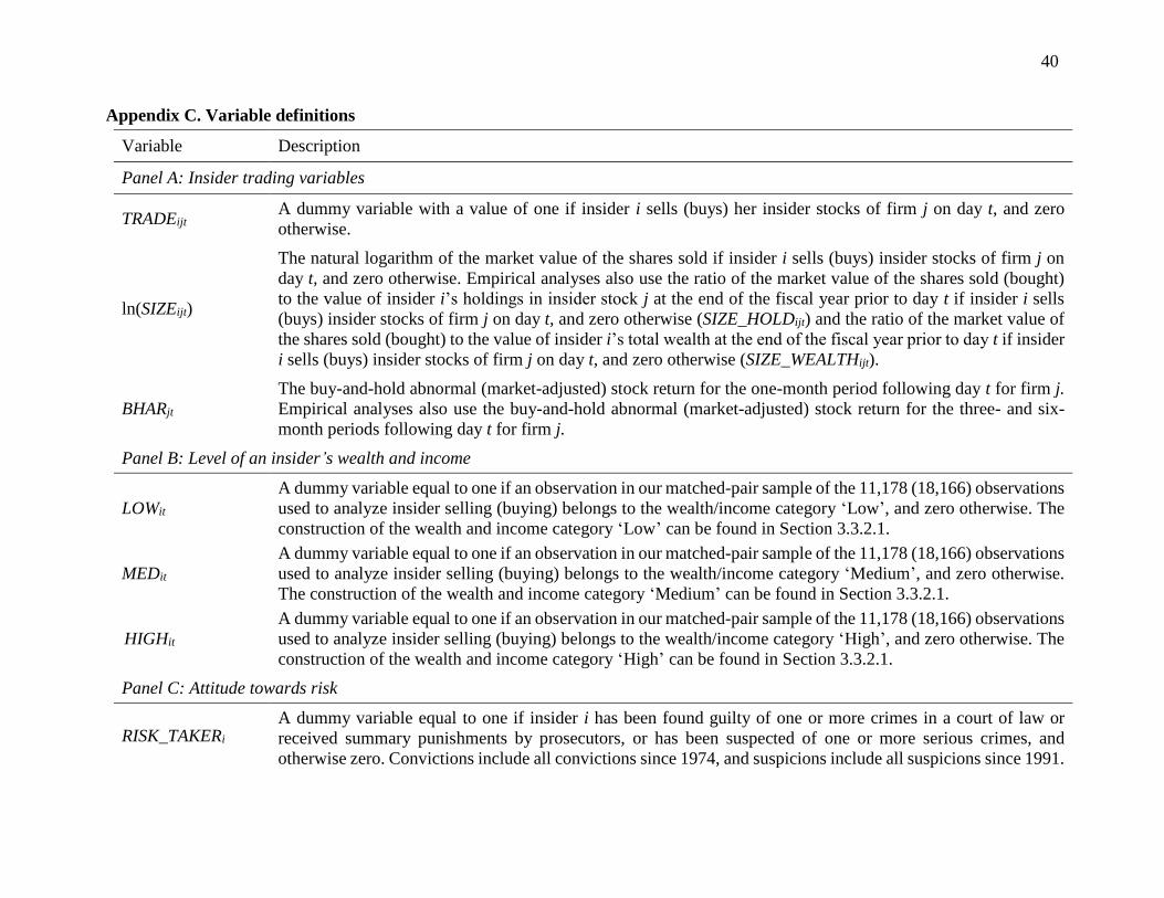
40

Appendix C. Variable definitions

Variable Description

Panel A: Insider trading variables

TRADEijt A dummy variable with a value of one if insider i sells (buys) her insider stocks of firm j on day t, and zero

otherwise.

ln(SIZEijt)

The natural logarithm of the market value of the shares sold if insider i sells (buys) insider stocks of firm j on

day t, and zero otherwise. Empirical analyses also use the ratio of the market value of the shares sold (bought)

to the value of insider i’s holdings in insider stock j at the end of the fiscal year prior to day t if insider i sells

(buys) insider stocks of firm j on day t, and zero otherwise (SIZE_HOLDijt) and the ratio of the market value of

the shares sold (bought) to the value of insider i’s total wealth at the end of the fiscal year prior to day t if insider

i sells (buys) insider stocks of firm j on day t, and zero otherwise (SIZE_WEALTHijt).

BHARjt

The buy-and-hold abnormal (market-adjusted) stock return for the one-month period following day t for firm j.

Empirical analyses also use the buy-and-hold abnormal (market-adjusted) stock return for the three- and six-

month periods following day t for firm j.

Panel B: Level of an insider’s wealth and income

LOWit

A dummy variable equal to one if an observation in our matched-pair sample of the 11,178 (18,166) observations

used to analyze insider selling (buying) belongs to the wealth/income category ‘Low’, and zero otherwise. The

construction of the wealth and income category ‘Low’ can be found in Section 3.3.2.1.

MEDit


used to analyze insider selling (buying) belongs to the wealth/income category ‘Medium’, and zero otherwise.

The construction of the wealth and income category ‘Medium’ can be found in Section 3.3.2.1.

HIGHit


used to analyze insider selling (buying) belongs to the wealth/income category ‘High’, and zero otherwise. The

construction of the wealth and income category ‘High’ can be found in Section 3.3.2.1.

Panel C: Attitude towards risk

RISK_TAKERi A dummy variable equal to one if insider i has been found guilty of one or more crimes in a court of law or

received summary punishments by prosecutors, or has been suspected of one or more serious crimes, and

otherwise zero. Convictions include all convictions since 1974, and suspicions include all suspicions since 1991.

41

Empirical analyses also use the natural logarithm of one plus the number of times insider i has been found guilty

of a crime in a court of law, received summary punishments by prosecutors or been suspected of a serious crime.

Panel D: Control variables

GENDERi A dummy variable equal to one if insider i is male, and zero otherwise.

ln(AGEi) The natural logarithm of the last two numbers of insider i’s birth year.

ln(1+TENUREijt) The natural logarithm of one plus the number of days since the beginning of insider i’s insider position in firm j

on day t.

CEOijt A dummy variable equal to one if insider i has an insider position as a CEO of firm j on day t, and zero otherwise.

EXECijt A dummy variable equal to one if insider i has an insider position as an executive other than CEO of firm j on

day t, and zero otherwise.

PROP_WEALTHijt The ratio of the value of insider i’s holdings in insider stock j at the end of the fiscal year prior to day t to the

value of insider i’s total wealth at the end of the fiscal year prior to day t.

ln(1+LIQUIDITYit)

The natural logarithm of one plus the value of insider i’s cash holdings at the end of a fiscal year prior to day t,

minus its time-series mean calculated for insider i over the sample period. As the variable LIQUIDITYit takes

both positive and negative values, we take the natural logarithm of one plus the absolute value of LIQUIDITYit

and then add back the original sign of LIQUIDITYit after taking the natural logarithm.

ln(1+NUMINSit) The natural logarithm of one plus the number of insider stocks owned by an insider i at the end of the fiscal year

prior to day t.

MOMENTUMit The buy-and-hold market-adjusted stock return for firm j for the six-month period prior to day t.

DECLOSSjt A dummy variable equal to one if the buy-and-hold market-adjusted stock return for the six-month period prior

to day t for firm j is negative and day t is in December, and zero otherwise.

ln(MVjt) The natural logarithm of the market value of shares for firm j multiplied by the number of shares outstanding

from the fiscal year prior to day t.

IVOLjt The standard deviation of the residuals from a market model regression estimated for firm j from 124 trading

days prior to day t to one trading day prior to day t.

PBjt The ratio of the market value of shares for firm j to the book value of equity from the fiscal year prior to day t.

RETjt The market-adjusted daily stock return for firm j on day t.

42

LEAD_kjt The market-adjusted daily stock return for firm j for each trading day during a five-trading-day period following

day t, k ϵ (1, 2, 3, 4, 5).

LAG_kjt The market-adjusted daily stock return for firm j for each trading day during a five-trading-day period prior to

day t, k ϵ (1, 2, 3, 4, 5).

ROAjt The ratio of annual earnings for firm j to total assets from the fiscal year prior to day t.

PREjt A dummy variable equal to one if day t is within a twenty-trading-day window prior to the quarterly earnings

announcement day for firm j, and zero otherwise.

POSTjt A dummy variable equal to one if day t is within a twenty-trading-day window following the quarterly earnings

announcement day for firm j, and zero otherwise.

YEAR_y The eight yearly dummy variables for the years 2000 to 2007.

FIRM_sj Dummy variables for each firm.

Notes:

All continuous variables are winsorized at the 1st and 99th percentiles of their distributions.

43

References

Acharya, V.V., Johnson, T.C., 2010. More insiders, more insider trading: Evidence from private-

equity buyouts. Journal of Financial Economics 98(3), 500-523.

Aggarwal, R., Erel, I., Stulz, R., Williamson, R., 2010. Differences in governance practices

between US and foreign firms: Measurement, causes, and consequences. Review of Financial

Studies 23(3), 3131-3169.

Ahern, K.R., 2017. Information networks: Evidence from illegal insider trading tips. Journal of

Financial Economics, forthcoming.

Alldredge, D.M., Cicero, D.C., 2015. Attentive insider trading. Journal of Financial Economics,

115(1), 84-101.

Amir, E., Kallunki, J.P., Nilsson, H., 2014. The association between individual audit partners’ risk

preferences and the composition of their client portfolios. Review of Accounting Studies 19(1),

103-133.

Atanasov, V., Ivanov, V., Litvak, K., 2012. Does reputation limit opportunistic behavior in the VC

industry? Evidence from litigation against VCs. Journal of Finance 67(6), 2215-2246.

Barber, B.M., Odean, T., 2001. Boys will be boys: Gender, overconfidence, and common stock

investment. The Quarterly Journal of Economics 116(1), 261-292.

Becker, G.S., 1968. Crime and punishment: An economic approach. Journal of Political Economy

78(2), 169-217.

Bénabou, R., Tirole, J., 2002. Self-confidence and personal motivation. The Quarterly Journal of

Economics, 871-915.

Beny, L.N., 2005. Do insider trading laws matter? Some preliminary comparative evidence.

American Law and Economics Review 7(1), 144-183.

44

Bertrand, M., Schoar, A., 2003. Managing with style: The effect of managers on firm policies. The

Quarterly Journal of Economics 118(4), 1169-1208.

Bhattacharya, U., Marshall, C.D., 2012. Do they do it for the money? Journal of Corporate

Finance 18(1), 92-104.

Boone, A.L., Floros, I.V., Johnson, S.A., 2016. Redacting proprietary information at the initial

public offering. Journal of Financial Economics 120(1), 102-123.

Brochet, F., 2010. Information content of insider trades before and after the Sarbanes-Oxley Act.

The Accounting Review 85(2), 419-446.

Brunnermeier, M.K., Parker, J.A., 2005. Optimal expectations. American Economic Review 95,

1092-1118.

Carhart, M.M., 1997. On persistence in mutual fund performance. The Journal of Finance 52(1),

57-82.

Cheng, Q., Lo, K., 2006. Insider trading and voluntary disclosures. Journal of Accounting

Research 44(5), 815-848.

Cohen, L., Malloy, C., Pomorski, L., 2012. Decoding inside information. Journal of Finance 67(3),

1009-1043.

Cronqvist, H., Makhija, A.K., Yonker, S.E., 2012. Behavioral consistency in corporate finance:

CEO personal and corporate leverage. Journal of financial economics 103(1), 20-40.

Dai, L., Parwada, J.T., Zhang, B., 2015. The governance effect of the media's news dissemination

role: Evidence from insider trading. Journal of Accounting Research 53(2), 331-366.

Davidson, R., Dey, A., Smith, A.J., 2016. Executives’ legal records and insider trading activities.

University of Chicago Working Paper.

Denis, D.J., Xu, J., 2013. Insider trading restrictions and top executive compensation. Journal of

Accounting and Economics 56(1), 91-112.

45

Ehrlich, I., 1973. Participation in illegitimate activities: A theoretical and empirical investigation.

Journal of Political Economy 81(3), 521-565.

Fama, E.F., French, K.R., 1993. Common risk factors in the returns on stocks and bonds. Journal

of Financial Economics 33(1), 3-56.

Fama, E.F., French, K.R., 2012. Size, value, and momentum in international stock returns. Journal

of Financial Economics 105(3), 457-472.

Garoupa, N., 2003. Behavioral economic analysis of crime: A critical review. European Journal

of Law and Economics 15, 5-15.

Gao, F., Lisic, L.L., Zhang, I.X., 2014. Commitment to social good and insider trading. Journal of

Accounting and Economics 57(2-3), 149-175.

Hillier, D., Korczak, A., Korczak, P., 2015. The impact of personal attributes on corporate insider

trading. Journal of Corporate Finance 30, 150-167.

Huddart, S., Ke, B., 2007. Information asymmetry and cross-sectional variation in insider trading.

Contemporary Accounting Research 24(1), 195-232.

Huddart, S., Ke, B., Shi, C., 2007. Jeopardy, non-public information, and insider trading around

SEC 10-K and 10-Q filings. Journal of Accounting and Economics 43(1), 3-36.

Iversen, H., Rundmo, T., 2002. Personality, risky driving and accident involvement among

Norwegian drivers. Personality and Individual Differences 33, 1251-1263.

Jagolinzer, A.D., Larcker, D.F., Taylor, D.J., 2011. Corporate governance and the information

content of insider trades. Journal of Accounting Research 49(5), 1249-1274.

Jeng, L.A., Metrick, A., Zeckhauser, R., 2003. Estimating the returns to insider trading: A

performance-evaluation perspective. Review of Economics and Statistics 85(2), 453-471.

Jin, L., Kothari, S.P., 2008. Effect of personal taxes on managers’ decision to sell their stock.

Journal of Accounting and Economics 46(1), 23-46.

46

Junger, M., West, R., Timman, R., 2001. Crime and Risky Behavior in Traffic: An Example of

Cross-Situational Consistency. Journal of Research in Crime and Delinquency 38, 439-459.

Kallunki, J-P., Nilsson, H., Hellström, J., 2009. Why do insiders trade? Evidence based on unique

data on Swedish insiders. Journal of Accounting and Economics 48(1), 37-53.

Kallunki, J.P., Mikkonen, J., Nilsson, H., Setterberg, H., 2016. Tax noncompliance and insider

trading. Journal of Corporate Finance 36, 157-173.

Kaplan, S.N., Klebanov, M.M., Sorensen, M., 2012. Which CEO characteristics and abilities

matter?. The Journal of Finance 67(3), 973-1007.

Karpoff, J., 2011. Does Reputation Work to Discipline Corporate Misconduct? In The Oxford

University Handbook of Corporate Reputation. Oxford University Press, Oxford, UK.

Ke, B., Huddart, S., Petroni, K., 2003. What insiders know about future earnings and how they use

it: Evidence from insider trades. Journal of Accounting and Economics 35(3), 315-346.

Klein, B., Leffler, K.B., 1981. The role of market forces in assuring contractual performance.

Journal of Political Economy, 615-641.

Korsell, L., 2001. Three decades of researching and combating economic crime: The Swedish case.

In S.A. Lindgren (Ed.), White-collar crime research. Old views and future potentials, pp. 91-

106. Stockholm: The National Council for Crime Prevention.

Kreps, D.M., Wilson, R., 1982. Reputation and imperfect information. Journal of Economic

Theory 27(2), 253-279.

Lakonishok, J., Lee, I., 2001. Are insider trades informative? Review of Financial Studies 14(1),

79-11.

MacLeod, W.B., 2007. Reputations, relationships, and contract enforcement. Journal of Economic

Literature 45, 595-628.

47

Malmendier, U., Tate, G., 2008. Who makes acquisitions? CEO overconfidence and the market's

reaction. Journal of financial Economics 89(1), 20-43.

Meulbroek, L.K., 1992. An empirical analysis of illegal insider trading. The Journal of Finance

47(5), 1661-1699.

Moeller, S.B., Schlingemann, F.P., Stulz, R.M., 2007. How do diversity of opinion and

information asymmetry affect acquirer returns?. Review of Financial Studies 20(6), 2047-2078.

Noe, C.F., 1999. Voluntary disclosures and insider transactions. Journal of Accounting and

Economics 27(3), 305-326.

Piotroski, J.D., Roulstone, D.T., 2005. Do insider trades reflect both contrarian beliefs and

superior knowledge about future cash flow realizations? Journal of Accounting and Economics

39(1), 55-81.

Piotroski, J.D., Roulstone, D.T., 2007. Evidence on the non-linear relation between insider trading

decisions and future earnings information. Journal of Law, Economics & Policy 4, 409.

Roulstone, D.T., 2003. The relation between insider‐trading restrictions and executive

compensation. Journal of Accounting Research 41(3), 525-551.

Rozeff, M.S., Zaman, M.A., 1998. Overreaction and insider trading: Evidence from growth and

value portfolios. Journal of Finance 53(2), 701-716.

Seyhun, H.N., 1986. Insiders’ profits, costs of trading, and market efficiency. Journal of financial

Economics 16(2), 189-212.

Seyhun, H.N., 1992. Effectiveness of the Insider-Trading Sanctions. Journal of Law & Economics

35, 149.

Seyhun, H.N., 1998. Investment intelligence from insider trading. MIT Press, Cambridge, MA.

Shapiro, C., 1983. Premiums for high quality products as returns to reputations. The Quarterly

Journal of Economics, 659-679.

48

Svensson, R., 2000. Strategic crimes – What type of crimes predict a future criminal career. Brå-

report. The Swedish National Council for Crime Prevention 3, 1-53.

Van den Steen, E., 2004. Rational overoptimism (and other biases). American Economic Review,

1141-1151.

49

Fig. 1.

This figure plots the probability for indifference between engaging (above the curve) and not engaging

(below the curve) in informed trading for varying levels of wealth and income (W) in three different

scenarios. In Scenario 1, an insider’s informed trading is subject to a low risk of legal enforcement and is

thus not likely to incur any fixed costs for the insider (d = 0), and also reputational damage and other

variable costs related to the magnitude of insider trading are small (c = 0.01). In Scenario 2, an insider’s

informed trading still involves a low risk of legal enforcement (d = 0), but includes larger reputational and

other variable costs (c = 0.06) than in Scenario 1. In Scenario 3, an insider’s informed trading is subject to

a high risk of legal enforcement and thus likely to incur large fixed costs (d = 1.0) and variable costs (c =

0.09) for the insider. In each of the three scenarios, we further set a = 0.5, r = 0.05 and σ = 5.0.

0%

10%

20%

30%

40%

50%

60%

70%

80%

0.2

50.5

0.7

51.0

1.2

51.5

1.7

52.0

2.2

52.5

2.7

53.0

3.2

53.5

3.7

54.0

4.2

54.5

4.7

55.0

5.2

55.5

5.7

56.0

6.2

56.5

6.7

57.0

7.2

57.5

7.7

58.0

Pro

bab

ilit

y f

or

ind

iffe

rence

, p

Insider's wealth and income level, W

Scenario 1

Scenario 2

Scenario 3

50

Fig. 2.

This figure plots the difference in the probability for indifference between engaging and not engaging in

informed trading between an insider with higher risk aversion (σ = 5.0) and an insider with lower risk

aversion (σ = 0.5) for varying levels of wealth and income (W) in three different scenarios. In Scenario 1,

we set d = 0 and c = 0.01. In Scenario 2, we set d = 0 and c = 0.06. In Scenario 3, we set d = 1.0 and c =

0.09. In all three scenarios, we further set a = 0.5 and r = 0.05.

0%

2%

4%

6%

8%

10%

12%

14%

0.2

50.5

0.7

51.0

1.2

51.5

1.7

52.0

2.2

52.5

2.7

53.0

3.2

53.5

3.7

54.0

4.2

54.5

4.7

55.0

5.2

55.5

5.7

56.0

6.2

56.5

6.7

57.0

7.2

57.5

7.7

58.0

Dif

fere

nce

in

th

e p

rob

abil

ity f

or

ind

iffe

ren

ce, p

Insider's wealth and income level, W

Scenario 1

Scenario 2

Scenario 3

51

Fig. 3.

This figure plots the mean buy-and-hold abnormal (market-adjusted) return over the one-month period

following the 5,589 and 9,083 insiders’ sales and purchases in the sample, respectively, in three categories

of the level of an insider’s wealth and income (‘Low’, ‘Medium’ and ‘High’). The abnormal returns

following purchases are multiplied by -1 to make the figure comparable to Fig. 1, i.e. higher insider returns

indicate that insiders are more cautious in their trading decisions. Refer to Section 3.3.2.1. and Appendix C

for the construction of the wealth and income categories. The sample includes all 3,388 insiders in all 393

listed firms in Sweden with at least one insider trade during the period 2000-2008.

-2,5%

-2,0%

-1,5%

-1,0%

-0,5%

0,0%

0,5%

1,0%

Low Medium High

Ab

no

rmal

Ret

urn

Insider's wealth and income level

Sell

Buy

52

Table 1 Summary statistics of insiders’ wealth and income, insider trading behavior and criminal behavior.

Percentiles

Mean S.D. Min 25th 50th 75th Max

Panel A: Wealth and income

Total wealth (thousands of SEK) 49,636.5 1,140,524.1 0.0 2,081.0 4,666.5 12,995.5 73,799,093.9

Annual income (thousands of SEK) 1,826.9 2,414.1 0.0 606.9 1,063.6 2,149.1 32,484.8

Panel B: Insider trading behavior

Insider sales (N=5,589)

Number of sales per insider 3.2 7.3 1.0 1.0 2.0 3.0 211.0

Trade size (thousands of SEK) 2,798.1 8,107.6 10.0 94.0 314.8 1,298.6 1,605,000.0

Trade size/insider holdings (%) 28.4 37.2 0.0 0.3 7.6 48.0 100.0

Trade size/total wealth (%) 14.7 25.0 0.0 1.3 4.2 14.1 100.0

Abnormal return (%) –0.4 12.9 –59.0 –7.4 –1.0 5.4 223.2

Insider purchases (N=9,083)

Number of purchases per insider 3.5 10.7 1.0 1.0 2.0 3.0 310.0

Trade size (thousands of SEK) 1,932.7 7,619.9 10.0 48.0 151.5 595.4 945,029.0

Trade size/insider holdings (%) 22.1 34.9 0.0 0.0 1.2 30.0 100.0

Trade size/total wealth (%) 7.5 18.2 0.0 0.5 1.6 5.1 100.0

Abnormal return (%) 2.1 12.3 –60.7 –4.5 1.0 7.3 227.9

Panel C: Criminal behavior

Number Percent

Convicted insiders 899 26.5

Non-convicted insiders 2,489 73.5

Total 3,388 100.0

Notes:

1. This table presents summary statistics of insiders’ wealth and income (Panel A), insider trading behavior (Panel B) and criminal behavior (Panel

C). The sample includes all 3,388 insiders in all 393 listed firms in Sweden with at least one insider trade over the sample period 2000-2008.

53

Panel A reports summary statistics on insiders’ total wealth and annual income based on the 6,582 insider-year observations in the sample.

Panel B reports summary statistics on insiders’ trading behavior in their insider stocks based on the 5,589 insider sale and the 9,083 insider

purchases in the sample. Panel C reports the frequency and percentage of insiders who have been convicted or suspected of a crime (convicted

insiders) and those who have not been convicted or suspected of a crime (non-convicted insiders).

2. Trade size is the market value of the shares traded. Abnormal return is the buy-and-hold abnormal (market-adjusted) stock return over a one-

month period following the trade. The means of the variables trade size and abnormal return are winsorized to the 1st and 99th percentiles of

their distributions. 1 SEK is equal to 0.12 USD during our sample period.

54

Table 2

Summary statistics of insider trading by the magnitude of the future abnormal return.

Abnormal return Mean profit/loss avoided Number of

insider trades

Proportion of trades made by insiders with different

levels of wealth and income (as percent of trades)

in thousands of

SEK

as percentage of total

wealth Low Medium High

Panel A: Insider sales (N=5,589)

≥ 0% 160.40 1.24 2,567 27.4 36.5 36.1

–0–5% –74.93 –0.33 1,215 28.7 33.3 38.0

–5–10% –128.46 –1.00 804 34.0 34.2 31.8

–10–15% –194.09 –1.78 482 35.9 32.6 31.5

–15–20% –171.78 –1.95 238 37.4 34.9 27.7

–20–25% –165.68 –2.92 121 48.8 32.2 19.0

–25–30% –262.99 –2.78 73 37.0 39.7 23.3

–30–35% –151.69 –4.03 42 45.2 38.1 16.7

–35–40% –243.78 –4.99 25 60.0 24.0 16.0

< –40% –204.44 –6.90 22 63.6 18.2 18.2

Panel B: Insider purchases (N=9,083)

≤ 0% –71.73 –0.55 4,185 27.1 36.5 36.4

0–5% 54.58 0.15 1,939 22.4 37.2 40.4

5–10% 136.61 0.59 1,272 25.7 34.9 39.4

10–15% 138.37 0.82 694 28.8 34.7 36.5

15–20% 158.21 1.52 361 30.7 32.7 36.6

20–25% 152.47 1.65 231 31.2 42.4 26.4

25–30% 185.78 1.43 119 34.5 39.5 26.0

30–35% 179.59 1.58 72 36.1 31.9 31.9

35–40% 190.46 2.84 45 26.7 48.9 24.4

> 40% 190.20 4.22 165 39.4 39.4 21.2

Notes:

55

1. Panel A (Panel B) presents summary statistics for the 5,589 insider sales (the 9,083 insider purchases) in the sample, summarized by the buy-

and-hold abnormal (market-adjusted) stock return over a one-month period following an insider trade. Profit/loss avoided is the market value

of the shares traded multiplied by the buy-and-hold abnormal stock return over a one-month period following the trade, expressed either in

thousands of SEK or as percentage of an insider’s total wealth. Insider trades are grouped into three categories based on the level of an insider’s

wealth and income (‘Low’, ‘Medium’ and ‘High’).

2. Refer to Section 3.3.2.1. and Appendix C for the construction of the wealth and income categories. The sample includes all 3,388 insiders in all

393 listed firms in Sweden with at least one insider trade over the period 2000-2008. Profit/loss avoided (in thousands of SEK) is winsorized to

the 1st and 99th percentiles of its distribution. 1 SEK is equal to 0.12 USD during our sample period.

56

Table 3 Descriptive statistics of the selected independent variables.

Variable Mean Median S.D. Min Max

Panel A: Insider selling (N=11,178)

LOWit 0.324 0.000 0.468 0.000 1.000

MEDit 0.351 0.000 0.477 0.000 1.000

HIGHit 0.324 0.000 0.468 0.000 1.000

RISKTAKERi 0.311 0.000 0.463 0.000 1.000

GENDERi 0.883 1.000 0.321 0.000 1.000

ln(AGEi) 3.977 3.989 0.179 2.996 4.454

ln(1+TENUREijt) 7.092 7.220 0.974 0.000 9.007

MOMENTUMjt 0.125 0.060 0.433 –0.665 2.112

PROP_WEALTHijt 0.256 0.062 0.338 0.000 1.000

DECLOSSjt 0.039 0.000 0.193 0.000 1.000

ln(1+LIQUIDITYit) –4.554 –11.031 11.636 –17.193 17.222

ln(1+NUMINSit) 0.719 0.693 0.463 0.000 2.197

CEOijt 0.094 0.000 0.291 0.000 1.000

EXECijt 0.459 0.000 0.498 0.000 1.000

PREjt 0.182 0.000 0.386 0.000 1.000

POSTjt 0.305 0.000 0.460 0.000 1.000

ln(MVjt) 0.132 0.000 2.131 –6.215 6.976

PBjt 3.529 2.311 3.609 0.364 20.527

ROAjt –0.019 0.042 0.279 –1.567 0.526

IVOLjt 0.032 0.026 0.019 0.001 0.106

Panel B: Insider buying (N=18,166)

LOWit 0.319 0.000 0.466 0.000 1.000

MEDit 0.361 0.000 0.480 0.000 1.000

HIGHit 0.319 0.000 0.466 0.000 1.000

RISKTAKERi 0.319 0.000 0.466 0.000 1.000

GENDERi 0.880 1.000 0.325 0.000 1.000

ln(AGEi) 3.967 3.970 0.188 2.996 4.407

ln(1+TENUREijt) 6.828 7.055 1.245 0.000 9.066

MOMENTUMjt 0.040 0.016 0.310 –0.674 1.208

PROP_WEALTHijt 0.148 0.020 0.257 0.000 1.000

ln(1+NUMINSit) 0.634 0.693 0.507 0.000 2.197

CEOijt 0.109 0.000 0.312 0.000 1.000

EXECijt 0.393 0.000 0.489 0.000 1.000

PREjt 0.172 0.000 0.377 0.000 1.000

POSTjt 0.339 0.000 0.473 0.000 1.000

ln(MVjt) 0.540 0.223 2.274 –6.215 6.976

PBjt 2.935 1.999 2.970 0.393 18.269

ROAjt –0.004 0.042 0.221 –1.159 0.508

IVOLjt 0.029 0.024 0.017 0.000 0.098

Notes:

57

1. The table reports descriptive statistics of the selected independent variables used in the analyses based

on our matched-pair sample of 5,589 (9,083) days with insider selling (buying) and 5,589 (9,083) days

without insider selling (buying). Panel A (Panel B) reports descriptive statistics for insider selling

(buying). The sample includes all 3,388 insiders in all 393 listed firms in Sweden with at least one

insider trade over the period 2000-2008. Refer to Appendix C for variable definitions. All continuous

variables are winsorized to the 1st and 99th percentiles of their distributions.

58

Table 4 Univariate analysis of how insiders with different levels of wealth and income time their insider trading.

All insiders Insiders with different levels of wealth and income

Low Medium High

Mean

(Median)

Mean

(Median)

Mean

(Median)

Mean

(Median)

Difference:

Low – High

Total wealth (thousands of SEK) 49,636.5

(4,666.5)

2,222.9

(1,930.1)

57,436.5

(4,993.7)

103,117.8

(16,214.2) –100,894.9

(–14,284.1)

Annual income (thousands of SEK) 1,826.9

(1,063.6)

602.5

(607.6)

1,535.8

(1,245.5)

3,944.0

(2,744.1)

–3,341.6

(–2,136.5)

Panel A: Insider selling

Days without insider selling 0.40%**

(–0.04%)

0.58%*

(–0.14%)

–0.03%

(–0.35%)

0.71%**

(0.26%**)

–0.13%

(–0.4%)

N=5,589 N=1,904 N=1,976 N=1,709

Days with insider selling –0.37%***

(–0.96%***)

–1.70%***

(–2.44%***)

–0.06%

(–0.39%)

0.50%***

(–0.50%)

–2.20%***

(–1.94%***)

N=5,589 N=1,721 N=1,952 N=1,916

Difference: Days without insider selling – Days with insider selling

Mean

(Median)

0.77%***

(0.92%***)

2.28%***

(2.30%***)

0.03%

(0.04%)

0.21%

(0.76%*)

Panel B: Insider buying

Days without insider buying 0.94%***

(0.36%***)

1.10%***

(0.23%**)

0.85%***

(0.45%***)

0.84%***

(0.44%***)

0.26

(–0.21%)

N=9,083 N=3,373 N=3,259 N=2,451

Days with insider buying 2.08%***

(0.97%***)

2.43%***

(0.98%***)

2.04%***

(0.90%***)

1.88%***

(1.02%***)

0.55%*

(–0.04%)

N=9,083 N=2,425 N=3,307 N=3,351

Difference: Days without insider buying – Days with insider buying

Mean

(Median)

–1.14%***

(–0.61%***)

–1.33%***

(–0.75%***)

–1.19%***

(–0.45%***)

–1.04%***

(–0.58%***)

59

Notes:

1. This table presents the results of univariate analysis to explore how insiders with different levels of wealth and income time their insider selling

(Panel A) and buying (Panel B). We first report the mean (median) values of insiders’ total wealth and annual income for insiders in the three

categories of the level of insiders’ wealth and income (‘Low’, ‘Medium’ and ‘High’). We then test whether the mean (median) future one-

month buy-and-hold abnormal (market-adjusted) returns are significantly different between the days with and without insider selling and

buying, respectively, in our matched-pair sample by using a two-tailed t-test (Wilcoxon rank-sum test). We conduct this analysis for insiders in

the three wealth and income categories. In addition, we test for difference in the mean (median) values of the future one-month abnormal returns

between the wealth and income categories ‘Low’ and ‘High’ by using a two-tailed t-test (Wilcoxon rank-sum test).

2. Refer to Section 3.3.2.1. and Appendix C for the construction of the wealth and income categories. The mean and median values of insiders’

total wealth and annual income are based on the 2,338, 2,542 and 1,702 insider-year observations in the categories ‘Low’, ‘Medium’ and ‘High’,

respectively. The sample includes all 3,388 insiders in all 393 listed firms in Sweden with at least one insider trade over the period 2000-2008.

3. 1 SEK is equal to 0.12 USD during our sample period. Significance at the 1%, 5%, and 10% (two-tailed) levels is indicated by ***, **, and *.

60

Table 5 Multivariate analysis of how insiders with different levels of wealth and income time their insider trading.

Panel A: Likelihood of

insider trading

Panel B: Magnitude of

insider trading

Selling Buying Selling Buying

Independent variables (1) (2) (3) (4)

LOWit×BHARjt –1.046**

(0.014)

–0.430

(0.230)

–5.017**

(0.027)

–1.574

(0.392)

MEDit×BHARjt 0.237

(0.589)

–0.433

(0.224)

1.660

(0.478)

–2.104

(0.232)

LOWit –0.058

(0.421)

–0.531***

(0.000)

–0.946**

(0.017)

–3.296***

(0.000)

MEDit –0.146**

(0.016)

–0.279***

(0.000)

–0.977***

(0.004)

–1.669***

(0.000)

RISK_TAKERi×BHARjt 0.569

(0.120)

0.298

(0.310)

3.135

(0.102)

1.494

(0.318)

BHARjt 0.064

(0.860)

0.849***

(0.006)

0.256

(0.896)

4.000***

(0.009)

RISK_TAKERi 0.205***

(0.000)

0.087**

(0.028)

1.286***

(0.000)

0.634***

(0.003)

GENDERi 0.554***

(0.000)

0.433***

(0.000)

3.506***

(0.000)

2.651***

(0.000)

ln(AGEi) 0.086

(0.574)*

–0.166

(0.151)

0.400

(0.637)

–0.437

(0.479)

ln(1+TENUREijt) 0.050*

(0.065)

–0.342***

(0.000)

0.348**

(0.029)

–1.602***

(0.000)

MOMENTUMjt 0.859***

(0.000)

–0.205***

(0.001)

4.432***

(0.000)

–0.776**

(0.018)

PROP_WEALTHijt 1.532***

(0.000)

–0.267***

(0.001)

8.234***

(0.000)

–1.287***

(0.003)

DECLOSSjt 0.553***

(0.000)

2.838***

(0.000)

ln(1+LIQUIDITYit) 0.001

(0.590)

0.009

(0.435)

ln(1+NUMINSit) 0.345

(0.000)

–0.005

(0.912)

2.015***

(0.000)

0.144

(0.500)

CEOijt –0.419

(0.000)

0.090

(0.144)

–2.164***

(0.000)

0.368

(0.243)

EXECijt 0.162

(0.007)

–0.452***

(0.000)

0.463

(0.167)

–2.946***

(0.000)

PREjt –1.003

(0.000)

–1.286***

(0.000)

–6.189***

(0.000)

–7.777***

(0.000)

POSTjt 0.433

(0.000)

0.519***

(0.000)

2.219***

(0.000)

2.637***

(0.000)

ln(MVjt) 0.248 –0.015 1.522*** 0.046

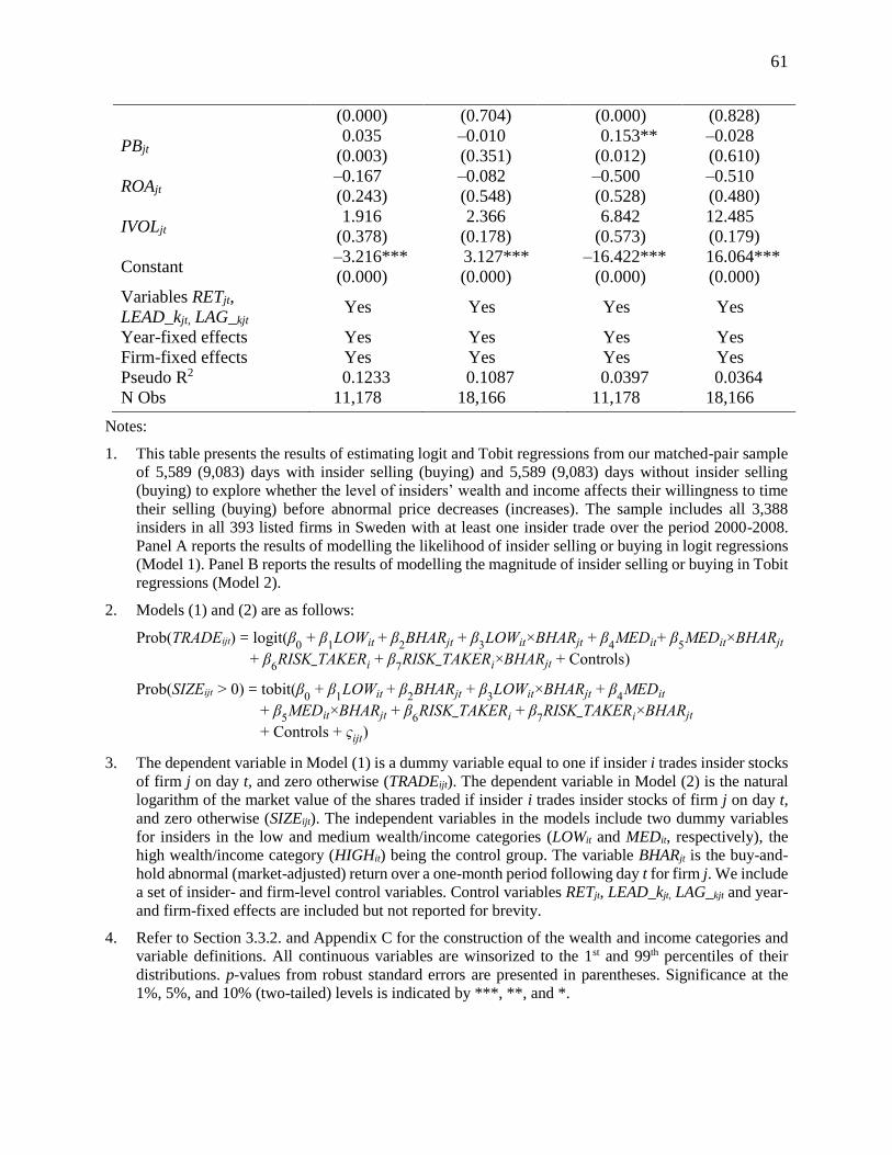
61

(0.000) (0.704) (0.000) (0.828)

PBjt 0.035

(0.003)

–0.010

(0.351)

0.153**

(0.012)

–0.028

(0.610)

ROAjt –0.167

(0.243)

–0.082

(0.548)

–0.500

(0.528)

–0.510

(0.480)

IVOLjt 1.916

(0.378)

2.366

(0.178)

6.842

(0.573)

12.485

(0.179)

Constant –3.216***

(0.000)

3.127***

(0.000)

–16.422***

(0.000)

16.064***

(0.000)

Variables RETjt,

LEAD_kjt, LAG_kjt Yes Yes

Yes Yes

Year-fixed effects Yes Yes Yes Yes

Firm-fixed effects Yes Yes Yes Yes

Pseudo R2 0.1233 0.1087 0.0397 0.0364

N Obs 11,178 18,166 11,178 18,166

Notes:

1. This table presents the results of estimating logit and Tobit regressions from our matched-pair sample

of 5,589 (9,083) days with insider selling (buying) and 5,589 (9,083) days without insider selling

(buying) to explore whether the level of insiders’ wealth and income affects their willingness to time

their selling (buying) before abnormal price decreases (increases). The sample includes all 3,388

insiders in all 393 listed firms in Sweden with at least one insider trade over the period 2000-2008.

Panel A reports the results of modelling the likelihood of insider selling or buying in logit regressions

(Model 1). Panel B reports the results of modelling the magnitude of insider selling or buying in Tobit

regressions (Model 2).

2. Models (1) and (2) are as follows:

Prob(TRADEijt) = logit(β0 + β

1LOWit + β

2BHARjt + β

3LOWit×BHARjt + β

4MEDit+ β

5MEDit×BHARjt

+ β6RISK_TAKERi + β

7RISK_TAKERi×BHARjt + Controls)

Prob(SIZEijt > 0) = tobit(β0 + β

1LOWit + β

2BHARjt + β

3LOWit×BHARjt + β

4MEDit


6RISK_TAKERi + β

7RISK_TAKERi×BHARjt

+ Controls + ςijt)

3. The dependent variable in Model (1) is a dummy variable equal to one if insider i trades insider stocks

of firm j on day t, and zero otherwise (TRADEijt). The dependent variable in Model (2) is the natural

logarithm of the market value of the shares traded if insider i trades insider stocks of firm j on day t,

and zero otherwise (SIZEijt). The independent variables in the models include two dummy variables

for insiders in the low and medium wealth/income categories (LOWit and MEDit, respectively), the

high wealth/income category (HIGHit) being the control group. The variable BHARjt is the buy-and-

hold abnormal (market-adjusted) return over a one-month period following day t for firm j. We include

a set of insider- and firm-level control variables. Control variables RETjt, LEAD_kjt, LAG_kjt and year-

and firm-fixed effects are included but not reported for brevity.

4. Refer to Section 3.3.2. and Appendix C for the construction of the wealth and income categories and

variable definitions. All continuous variables are winsorized to the 1st and 99th percentiles of their

distributions. p-values from robust standard errors are presented in parentheses. Significance at the

1%, 5%, and 10% (two-tailed) levels is indicated by ***, **, and *.

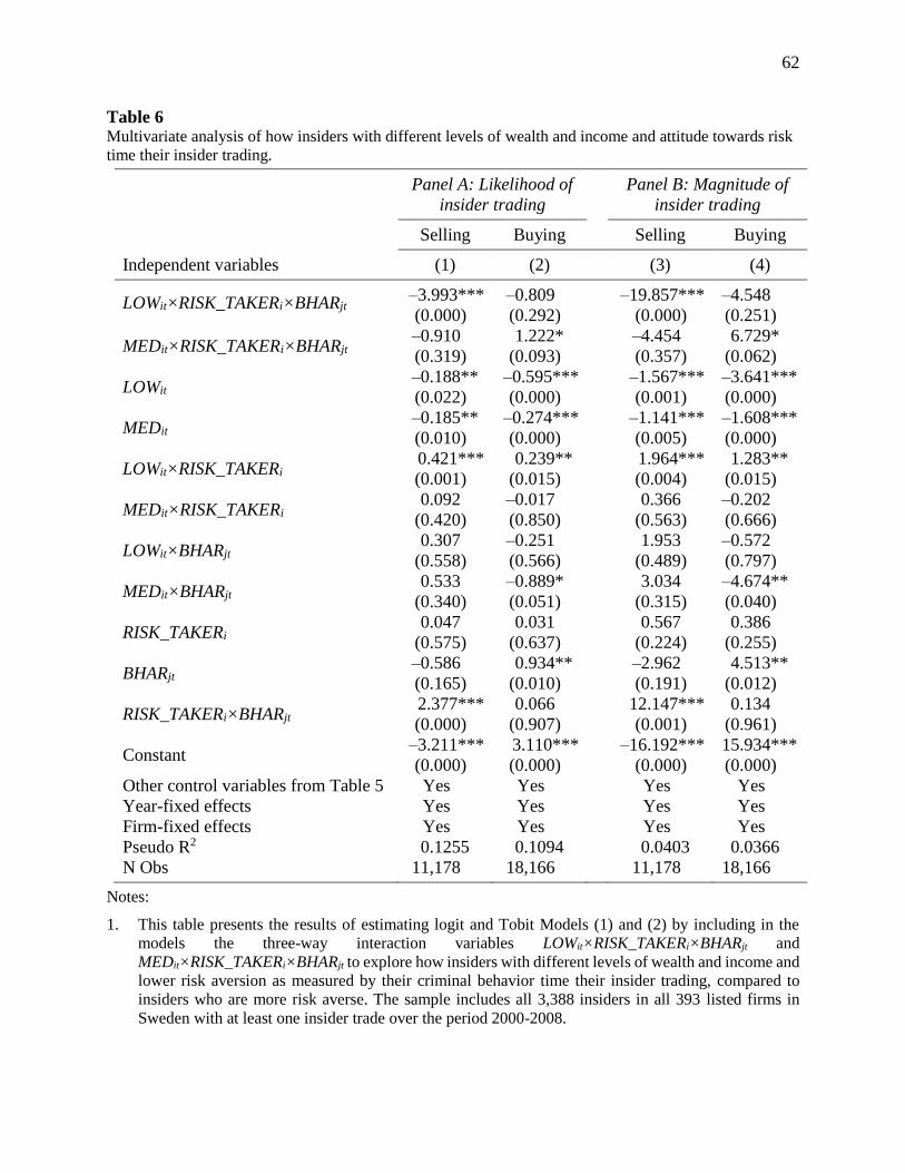
62

Table 6 Multivariate analysis of how insiders with different levels of wealth and income and attitude towards risk

time their insider trading.

Panel A: Likelihood of

insider trading

Panel B: Magnitude of

insider trading

Selling Buying Selling Buying

Independent variables (1) (2) (3) (4)

LOWit×RISK_TAKERi×BHARjt –3.993***

(0.000)

–0.809

(0.292)

–19.857***

(0.000)

–4.548

(0.251)

MEDit×RISK_TAKERi×BHARjt –0.910

(0.319)

1.222*

(0.093)

–4.454

(0.357)

6.729*

(0.062)

LOWit –0.188**

(0.022)

–0.595***

(0.000)

–1.567***

(0.001)

–3.641***

(0.000)

MEDit –0.185**

(0.010)

–0.274***

(0.000)

–1.141***

(0.005)

–1.608***

(0.000)

LOWit×RISK_TAKERi 0.421***

(0.001)

0.239**

(0.015)

1.964***

(0.004)

1.283**

(0.015)

MEDit×RISK_TAKERi 0.092

(0.420)

–0.017

(0.850)

0.366

(0.563)

–0.202

(0.666)

LOWit×BHARjt 0.307

(0.558)

–0.251

(0.566)

1.953

(0.489)

–0.572

(0.797)

MEDit×BHARjt 0.533

(0.340)

–0.889*

(0.051)

3.034

(0.315)

–4.674**

(0.040)

RISK_TAKERi 0.047

(0.575)

0.031

(0.637)

0.567

(0.224)

0.386

(0.255)

BHARjt –0.586

(0.165)

0.934**

(0.010)

–2.962

(0.191)

4.513**

(0.012)

RISK_TAKERi×BHARjt 2.377***

(0.000)

0.066

(0.907)

12.147***

(0.001)

0.134

(0.961)

Constant –3.211***

(0.000)

3.110***

(0.000)

–16.192***

(0.000)

15.934***

(0.000)

Other control variables from Table 5 Yes Yes Yes Yes

Year-fixed effects Yes Yes Yes Yes

Firm-fixed effects Yes Yes Yes Yes

Pseudo R2 0.1255 0.1094 0.0403 0.0366

N Obs 11,178 18,166 11,178 18,166

Notes:

1. This table presents the results of estimating logit and Tobit Models (1) and (2) by including in the

models the three-way interaction variables LOWit×RISK_TAKERi×BHARjt and

MEDit×RISK_TAKERi×BHARjt to explore how insiders with different levels of wealth and income and

lower risk aversion as measured by their criminal behavior time their insider trading, compared to

insiders who are more risk averse. The sample includes all 3,388 insiders in all 393 listed firms in

Sweden with at least one insider trade over the period 2000-2008.

63

2. In Panel A, the dependent variable is a dummy variable that equals one if insider i trades her insider

stocks on day t, and zero otherwise (TRADEijt). In Panel B, the dependent variable is the natural

logarithm of the value of the trade if insider i trades insider stocks of firm j on day t, and zero otherwise

(SIZEijt). The dummy variables LOWit and MEDit equal one for insiders in the low and medium

wealth/income categories, respectively, the high wealth and income category (HIGHit) being the

control group. The dummy variable RISK_TAKERi measures an insider’s lower risk aversion and

equals one for insiders who have been convicted or suspected of crimes, and zero otherwise. The

variable BHARjt is the buy-and hold abnormal (market-adjusted) return over a one-month period

following day t for firm j. Insider- and firm-level control variables from Table 5 and year- and firm-

fixed effects are included in all regressions but are not tabulated for the sake of brevity.

3. Refer to Section 3.3.2. and Appendix C for the construction of the wealth and income categories and

variable definitions. All continuous variables are winsorized to the 1st and 99th percentiles of their

distributions. p-values from robust standard errors are presented in parentheses. Significance at the

1%, 5%, and 10% (two-tailed) levels is indicated by ***, **, and *.

64

Table 7 Percentage monthly returns earned on portfolios formed on the basis of insider trading by insiders with different levels of wealth and income.

Portfolio Monthly

mean

number of

insider trades

Mean

raw

return

Mean

market-

adjusted

return

Intercept from Coefficient estimates for the four-factor

model

CAPM Three-

factor

Four-

factor Rmt – Rft SMBt HMLt PMOMt R2

(1) (2) (3) (4) (5) (6) (7) (8) (9) (10) (11) (12)

Panel A: Insider selling (N=105 months)

LOWpt 16 –2.15 –1.59**

(–2.25)

–2.59***

(–3.14)

–1.95**

(–2.30)

–2.32**

(–2.51)

0.77***

(3.40)

0.19

(0.35)

–0.55*

(–1.77)

0.32

(1.52) 0.213

MEDpt 18 –0.98 –0.18

(–0.27)

–1.47*

(–1.73)

–0.70

(–0.72)

–0.67

(–0.70)

0.85***

(5.19)

0.33

(0.76)

–0.70***

(–2.72)

–0.03

(–0.15) 0.259

HIGHpt 18 –0.67 –0.03

(–0.06)

–1.12

(–1.52)

–0.45

(–0.51)

–0.66

(–0.72)

0.76***

(3.94)

0.33

(0.96)

–0.59*

(–1.68)

0.18

(1.35) 0.306

LOWpt –

HIGHpt 34

–1.49**

(–2.36)

–1.56**

(–2.55)

–1.47**

(–2.08)

–1.49**

(–2.07)

–1.66**

(–2.39)

0.01

(0.04)

–0.14

(–0.41)

0.04

(0.16)

0.14

(0.74) 0.010

Panel B: Insider buying (N=108 months)

LOWpt 22 2.75

2.99***

(4.99)

2.55***

(3.69)

3.33***

(4.49)

3.67***

(5.09)

0.48***

(3.55)

0.27

(0.91)

–0.76***

(–3.09)

–0.30*

(–1.88) 0.263

MEDpt 31 2.33 2.47***

(4.96)

2.13***

(3.35)

2.53***

(3.53)

2.78***

(3.96)

0.53***

(3.32)

0.08

(0.26)

–0.39**

(–1.99)

–0.22

(–1.45) 0.243

HIGHpt 31 1.89

2.12***

(4.43)

1.68***

(2.84)

1.81***

(2.70)

2.00***

(3.02)

0.39***

(2.86)

0.21

(0.90)

–0.16

(–0.89)

–0.16

(–1.28) 0.168

LOWpt –

HIGHpt 53

0.85

(1.40)

0.87

(1.45)

0.87

(1.29)

1.52**

(2.45)

1.68***

(2.66)

0.09

(0.69)

0.06

(0.24)

–0.60***

(–3.08)

–0.14

(–0.89) 0.088

Notes:

1. This table presents percentage monthly returns earned on portfolios formed according to insider selling (Panel A) and insider buying (Panel B)

by insiders with different levels of wealth and income. We calculate the returns for each of the three portfolios as follows. For each calendar

month between January 2000 through December 2008, we calculate, for each wealth and income category (‘Low’, ‘Medium’ and ‘High’), the

mean raw return over the one-month period following each insider trade date over all insider trades during the month. Raw returns are the mean

percentage monthly returns earned by each portfolio. Market-adjusted returns are the mean raw return less the return on an equally weighted

market index. The CAPM intercept is the estimated intercept from a time-series regression of the portfolio return (Rt – Rft) on the market excess

65

return (Rmt – Rft). The intercept for the Fama-French three-factor model is the estimated intercept from a time-series regression of the portfolio

return on the market excess return (Rmt – Rft), a zero investment size portfolio (SMBt), and a zero-investment book-to-market portfolio (HMLt).

The four-factor model intercept is estimated by adding a zero-investment price momentum portfolio (PMOMt) as an independent variable. The

final line shows the difference in returns between portfolios LOWpt and HIGHpt. The mean monthly number of insider trades in each portfolio

is also reported. Newey-West (1987) adjusted t-statistics appear in parentheses below the returns and the coefficient estimates. Each t-statistic

pertains to the null hypothesis that the associated return or coefficient is zero, expect for the t-statistic on the coefficient estimate of (Rmt – Rft)

for portfolios LOWpt, MEDpt and HIGHpt, for which the null hypothesis is that the coefficient is one.

2. Refer to Section 3.3.2.1. and Appendix C for the construction of the wealth and income categories ‘Low’, ‘Medium and ‘High’. The sample

includes insider trades by 3,388 insiders in 393 listed firms in Sweden over the period 2000-2008. For insider selling, we lose 3 out of a total

108 sample months because we require that, for each calendar month, there are insider sales (purchases) in all the three wealth and income

categories. Significance at the 1%, 5%, and 10% (two-tailed) levels is indicated by ***, **, and *.

66

Table 8 Abnormal returns following insider selling by the proportion of an insider’s wealth allocated to insider stock.

Notes:

1. This table reports the mean (median) one-month buy-and-hold abnormal (market-adjusted) returns

following the 5,589 insider sales in the sample made by insiders with different levels of wealth and income

(‘Low’, ‘Medium’ and ‘High’), broken into quartiles based upon the proportion of an insider’s total wealth

allocated to her insider stock (Q1 – Q4). Quartile 1 (4) includes insider sales by insiders who have

allocated less (more) of their wealth to their insider stock prior to selling them. In each quartile group (Q1

– Q4), we test for difference in the mean (median) future one-month abnormal returns between the wealth

and income categories ‘Low’ and ‘High’ by using a two-tailed t-test (Wilcoxon rank-sum test). In

addition, in each wealth and income category, we test for difference in the mean (median) future one-

month abnormal returns between the quartile groups 1 and 4 by using a two-tailed t-test (Wilcoxon rank-

sum test).

2. Refer to Section 3.3.2.1. and Appendix C for the construction of the wealth and income categories. The

sample includes all 3,388 insiders in all 393 listed firms in Sweden with at least one insider trade over the

period 2000-2008. Significance at the 1%, 5%, and 10% (two-tailed) levels is indicated by ***, **, and

*.

Quartile of the proportion

of an insider’s wealth

allocated to insider stock

All insiders Insiders with different levels of wealth and

income

Low Medium High

Mean

(Median)

Mean

(Median)

Mean

(Median)

Mean

(Median)

Difference:

Low – High

Quartile 1

(less wealth allocated)

0.07%

(–0.83%**)

–1.09%***

(–2.17%***)

0.44%

(–0.49%)

1.09%

(–0.51%)

–2.18%**

(–1.66%***)

N=1,276 N=457 N=462 N=357

Quartile 2 0.12%

(0.12%)

–1.79%***

(–0.10%**)

0.78%

(0.80%)

1.12%**

(0.40%)

–2.91%***

(–0.50%***)

N=990 N=305 N=301 N=384

Quartile 3 –0.47%

(–1.08%***)

–1.78%***

(–2.93%***)

–0.15%

(–0.97%**)

0.29%

(–0.23%)

–2.07%***

(–2.70%***)

N=1,491 N=441 N=497 N=553

Quartile 4

(more wealth allocated)

–0.86%***

(–1.69%***)

–2.10%***

(–3.16%***)

–0.70%

(–0.73%**)

–0.02%

(–1.05%**)

–2.08%**

–2.11%***)

N=1,832 N=518 N=692 N=622

Difference: Q1 – Q4

Mean 0.93%* 1.01% 1.14% 1.11%

(Median) (0.86%*) (0.99%) (0.24%) (0.54%*)

do an insider’s wealth and income matter in the decision ... · do an insider’s wealth and...

Documents