The Importance of Bureaucrats in a Weak State

Evidence from the Philippines∗

Mark Dincecco† Nico Ravanilla‡

May 8, 2017

Abstract

We present new evidence about the quantitative extent to which individual bureaucrats

matter for public sector performance in a developing country context where the state is

weak. We construct revenue district office-matched panel data for the Philippines that

allow us to follow tax officers across different assignments. We demonstrate that bu-

reaucrat fixed effects explain a significant extent of differences in local tax outcomes.

Furthermore, we show evidence consistent with the view that political patronage nega-

tively influences bureaucrat behavior, and that the bureaucratic leader attempts to miti-

gate revenue loss due to such patronage through more effective officer-district matching.

Our results provide new insights into the inner workings of government in the develop-

ing world.

∗We thank Cesi Cruz, Sean Gailmard, Alberto Simpser, and seminar participants at the University of Michigan

and MPSA 2016 for valuable comments. We thank Karl Chua for generously sharing tax officer assignment

data, and Marianne Juco for outstanding research assistance.†University of Michigan; dincecco@umich.edu‡University of California, San Diego; nravanilla@ucsd.edu

1

1 Introduction

A well-organized bureaucracy staffed by qualified and motivated individuals is a classic

hallmark of high state capacity (Weber, 1922). In this idealized world, the bureaucracy

should be able to effectively implement the government’s policy goals. Furthermore, indi-

vidual bureaucrats should not make much of a difference to public sector outcomes, because

bureaucratic performance should be relatively good across the board.

In an actual developing country context in which the state is weak, however, the bureau-

cracy’s ability to carry out the government’s mandated policy may fall far short of this tra-

ditional ideal. This paper evaluates a central question about bureaucracy that may emerge

in the weak state context. To what extent do individual bureaucrats matter for public sector

performance?

To answer, we analyze bureaucratic performance in the Philippines. Our main goal is to

quantify the amount (if any) that individual tax bureaucrats actually contribute to observed

differences in revenue collection – a core state function (Levi, 1988) and a key measure of

public sector performance. Bureaucrat-specific effects may be correlated with other local

features, making it difficult to disentangle the true role of individual bureaucrats. To test for

the potential importance of bureaucrats, we construct new revenue district office-matched

panel data for the Philippines that allow us to track the same tax officers across different

assignments over time. Our data enable us to control for observable and unobservable dif-

ferences across district offices. Thus, we can estimate the extent of unexplained variation in

district-level revenue outcomes that bureaucrat fixed effects can account for after control-

ling for district office fixed effects and time-varying district office features. To the best of our

knowledge, this type of analysis is the first of its kind to evaluate the fiscal role of individual

bureaucrats.

The results of our investigation indicate that individual bureaucrats matter to a signifi-

cant quantitative extent for fiscal performance outcomes in the weak state context. Including

bureaucrat fixed effects significantly increases adjusted R2 values in regression models that

already control for observable and unobservable district office features. The fiscal differ-

2

ences between individual bureaucrats are large. A tax officer in the bottom quartile of the

distribution for the total tax take reduces revenue collection by P1.6 billion (more than $37

million), while one in the top quartile increases it by P1.9 billion (more than $44 million).

We show that our results are robust to district-level differences in revenue potential, serial

correlation, the importance of Metro Manila, the active influence of bureaucrats, and the

persistence of bureaucratic quality across office assignments.

We next explore the factors that influence bureaucratic behavior when the state is weak.

We briefly draw on anecdotal evidence about public perceptions of bureaucratic corruption

in the Philippines. We then evaluate the extent to which tenure length influences revenue

collection, finding that more senior tax officers – who may be politically well-connected –

collect significantly less tax revenues. Overall, this analysis is consistent with the view that

political patronage influences the behavior of individual bureaucrats in ways that hinder

public sector performance. To conclude our investigation, we show evidence that the rel-

evant bureaucratic leader – namely, the Commissioner of the Bureau of Internal Revenue

(BIR) – attempts to mitigate revenue loss due to political patronage through more effective

officer-district matching.

Our paper offers new evidence about the inner workings of government in the develop-

ing world. To improve our knowledge of the policy process, Dixit (2010) argues that schol-

ars must open the “black box” of public administration in the same way that economists

began to study the internal dynamics of firms.1 Rauch and Evans (2000) find a positive re-

lationship between professional bureaucracies and state capacity across 30-plus developing

nations. Cruz and Keefer (2015) show evidence that patronage politics prevents public sec-

tor reforms across more than 400 World Bank loans in 100-plus countries. Still, there are

relatively few works that analyze how government operates at the micro level. This nascent

literature generally tests the selection, incentive structure, or monitoring of bureaucrats (Fi-

nan, Olken and Pande, 2015).2 Our paper contributes to this nascent literature by analyzing

1Our research design builds on Bertrand and Schoar (2003), who show evidence that individual top managerssignificantly influence corporate decision-making.

2For example, Iyer and Mani (2012) find that politicians exert significant influence over the process of bu-reaucratic transfers in India. Rasul and Rogger (Forthcoming) show evidence that managerial autonomy by

3

a more basic – and in this regard, more fundamental – question: to what quantitative ex-

tent (if any) do individual bureaucrats actually matter to fiscal performance outcomes in the

weak state context?

In this respect, our paper also contributes to the recent literature on state capacity and

economic development. Capable states may play productive developmental roles through

the provision of public goods including law and order, property rights protections, trans-

portation infrastructure, and mass education (Besley and Persson, 2011). Scholars find sig-

nificant relationships between institutions that promote state strength and economic growth

across a wide range of contexts.3 However, this literature tends to ignore the role of individ-

ual bureaucrats. A related literature explicitly links bureaucratic quality and development

outcomes. Evans and Rauch (1999) relates bureaucratic effectiveness to economic growth

across the developing world. Cingolani, Thomsson and de Crombrugghe (2015) show cross-

country evidence that bureaucratic autonomy is correlated with better health outcomes. Yet

this literature tends to treat bureaucrats as homogeneous. Our paper contributes to this

body of research by analyzing how (heterogenous) individual bureaucrats may influence

public sector performance in the developing world.4

We structure this paper as follows. Section 2 explains why individual bureaucrats are

particularly likely to matter for public sector outcomes in the weak state context. Section

3 provides an overview of the Philippine tax system. Section 4 describes the data. Section

5 presents the empirical strategy and main results for the importance of bureaucrat fixed

effects. Section 6 performs robustness checks. Sections 7 and 8 investigate how political

patronage may influence bureaucratic behavior. Section 9 concludes.

bureaucrats improves project completion rates in Nigeria. Dal Bo, Finan and Rossi (2013) show experimentalevidence that higher wages improve the quality and quantity of public sector applicants in Mexico. Callenet al. (2015) show experimental evidence that the personality traits of health workers affect public health out-comes in Pakistan. Gulzar and Pasquale (2015) find that local public service delivery in India improves whenbureaucratic and electoral borders are well-aligned.

3Such contexts include Asia (Wade, 1990, Evans, 1995, Dell, Lane and Querubin, 2015), European history(Dincecco and Katz, 2016), Latin America (Centeno, 2002, Acemoglu, Garcia-Jimeno and Robinson, 2015),Sub-Saharan Africa (Herbst, 2000, Gennaioli and Rainer, 2007, Michalopoulos and Papaioannou, 2013), andbetween countries (Besley and Persson, 2011, Dincecco and Prado, 2012).

4In a related manner, Denizer, Kaufmann and Kraay (2013) evaluate the importance of individual project man-agers for World Bank projects, showing evidence that project manager quality is significantly correlated withproject outcomes.

4

2 Why Individual Bureaucrats May Matter

This section develops a simple conceptual framework that will guide our empirical analysis.

First, we describe the public sector’s unique institutional features. Second, we analyze how

such features may interact with low state capacity to influence public sector performance.

2.1 Institutional Features of the Public Sector

A state’s tax policy typically derives from a combination of constitutional, legislative, and

executive choices. However, it is up to individual tax bureaucrats to implement whatever

the state’s mandated policy is.

There are several institutional features particular to the state (versus the private sector)

which may influence the extent to which individual tax bureaucrats are willing and able to

implement this policy.5 First, the state’s tax authority is (relatively) unrivaled.6 The state

typically faces non-existent or muted “competition” over taxation. A lack of outside com-

petition may make it more difficult for the state to exploit basic incentive schemes (e.g.,

service volume) that can motivate individual tax bureaucrats to effectively carry out ser-

vice tasks. Furthermore, this lack of outside competition may make self-monitoring by the

state important. Individual tax bureaucrats, however, may rotate between service tasks and

the monitoring of colleagues, which may corrupt monitoring incentives. Second, the gov-

ernment does not typically provide performance-based monetary incentives, because such

incentives may induce a multitasking problem whereby a bureaucrat emphasizes the part of

the work with monetary incentives rather than the other – potentially important, but difficult

to incentivize – parts. Third, politicians may try to influence bureaucratic behavior through

promotion or punishment schemes or award bureaucratic posts to (unqualified) supporters.

A politician will only indirectly bear the cost of a less effective bureaucracy through a lower

probability of future re-election (i.e., under democracy).7 All three institutional features –

5We base this discussion on Finan, Olken and Pande (2015).6Also, the government’s fiscal time horizon is typically long (it will likely collect revenues far into the future,regardless of any regime change), which may influence its workplace policy.

7For this reason, there are often formal rules that attempt – with varying levels of success – to limit the ability

5

unrivaled competition, the lack of monetary incentives, and political patronage – may neg-

atively affect the performance of individual tax bureaucrats. Finally, individuals that decide

to work in government may have a strong intrinsic belief in public service, which may im-

prove their performance. However, intrinsic motivation may vary among individual tax

bureaucrats.8

2.2 The Role of State Capacity

We now analyze how the public sector’s unique institutional features may interact with low

state capacity to influence the performance of individual bureaucrats. Here we conceptu-

alize “state capacity” as the ability of the bureaucracy to accomplish its intended actions.9

This conceptualization makes sense, because bureaucratic capacity represents a core aspect

of the state’s “infrastructural power” (Mann, 1984).10

According to the traditional ideal (Weber, 1922), the bureaucratic leader should be able

to effectively implement the government’s mandated tax policy. Due to “rational” bureau-

cratic organization, the bureaucratic leader will be relatively well-placed to overcome the

unique institutional features of the public sector (i.e., unrivaled competition, lack of mone-

tary incentives, political patronage) that may negatively affect the performance of individ-

ual bureaucrats. Since bureaucratic performance should be relatively good across the board,

individual tax bureaucrats should not make much of a difference with respect to revenue

collection. Thus, in this idealized world, it is relatively unlikely that bureaucratic transfers

between districts will have significant effects on revenue collection. Furthermore, the scope

for (endemic) corruption should be relatively small.

In an actual developing country context in which the state is weak, however, the bureau-

cracy’s ability to effectively implement the government’s stated policy may fall far short

of politicians to affect bureaucratic employment decisions.8For example, Hanna and Wang (2013) show experimental evidence that dishonest individuals are more likelyto want to enter government.

9We base this conceptualization on Huber and McCarty (2004) and Acemoglu, Garcia-Jimeno and Robinson(2015).

10Weber (1922), Huntington (1968), Skocpol (1979), and Evans (1995) also highlight the importance of the bu-reaucracy for state capacity.

6

of this classic ideal (Huber and McCarty, 2004).11 Such a bureaucracy may not be well-

organized, making it difficult for the bureaucratic leader to control the rank-and-file. Indi-

vidual tax bureaucrats themselves may lack the ability to effectively carry out orders. Fur-

thermore, the tax administration may not have enough resources to effectively execute the

agreed-upon policy. Finally, the lack of effective oversight and/or political patronage may

encourage corrupt behavior by individual tax bureaucrats.

Thus, relative to the Weberian ideal, it may be particularly difficult for the bureaucratic

leader to overcome the public sector’s unique institutional features and effectively imple-

ment the government’s tax policy when the state is weak. In this context, individual dif-

ferences between bureaucrats – for example, in terms of political patronage – may be more

likely to surface. Thus, in contrast to the classic description, individual tax bureaucrats may

now make quite a difference with respect to revenue collection. In turn, officer transfers

between districts may now significantly affect revenue collection. Political patronage by

individual bureaucrats may also now be more likely to be endemic.

Note that the performance of individual tax bureaucrats may be relatively poor in the

weak state context even if the bureaucratic leader is well-qualified and scrupulous (Huber

and McCarty, 2004). For example, this leader may be able to articulate a clear and ratio-

nal revenue collection policy. However, the effective implementation of such a policy may

be difficult due to quality variations and/or incentives for political patronage among the

rank-and-file. Thus, the main problem in the weak state context may not be the lack of

high-level policy know-how, but rather the rank-and-file’s poor ability and/or inclination

to implement the agreed-upon policy. Our empirical analysis will analyze how the bureau-

cratic leader may use more effective officer-district matching to help mitigate the revenue

loss due to underperformance by individual bureaucrats.

11To be clear, the bureaucracy’s actual ability to carry out public policy may fall short of the Weberian idealeven when state capacity is relatively high (e.g., Lipsky, 1980, Carpenter, 2001). Still, we focus our analysison the weak state context, where bureaucratic organization may be particularly problematic.

7

2.3 Predictions

Our simple conceptual framework produces a key prediction about the performance of in-

dividual tax bureaucrats when the state is weak. Namely, individual bureaucrats are likely

to make a significant difference in revenue collection. Our framework also suggests that

political patronage is likely to influence the behavior of individual tax bureaucrats. In what

follows, we will evaluate both predictions for the Philippines.

3 Taxation in the Philippines

3.1 Bureau of Internal Revenue

The Bureau of Internal Revenue (BIR) is the main revenue agency of the Philippines. The for-

mal objective of BIR is to collect internal tax revenues on behalf of the national government.

BIR is responsible for the collection of roughly 75 percent of total annual taxes.12

The Commissioner of Internal Revenue, a presidential appointee, heads BIR. The Com-

missioner, in turn, delegates powers to BIR officials of at least the rank of revenue district

officers (RDO) via the issuance of revenue memorandum orders (RMOs). RDOs exercise the

power to assess and collect taxes at the local level.

Each RDO heads a revenue district office, of which there are 115 spread throughout the

country. Together, RDOs are responsible for the collection of roughly 50 percent of annual

internal tax revenues (which amounts to nearly 5 percent of annual GDP).13 Each revenue

district approximately covers one province or one city. High-revenue areas may have mul-

tiple revenue district offices. Metro Manila offices, of which there are 26, collect roughly

70 percent of all annual RDO-generated revenue. Given Metro Manila’s importance, our

empirical analysis ahead will test it separately for robustness.

12The remaining 25 percent of national-level taxes are collected by the Bureau of Customs, the Land Trans-portation Office, and other national agencies.

13The remaining internal tax revenues are collected from the country’s 1,300 largest corporations by BIR’sLarge Taxpayers Service.

8

3.2 Fiscal Performance

Panel A of Table 1 breaks down BIR’s total tax take by major tax type.14 Total tax revenues

averaged roughly 10 percent of GDP per year over 2002-2007, the period for which district-

level fiscal data (which we will describe in Section 4) are available. This relatively low share

is consistent with what we would expect in the weak state context (Besley and Persson,

2011). Corporate income taxes (CIT) accounted for the largest BIR tax share (roughly 3 per-

cent of GDP). CIT evasion is widespread among small corporate taxpayers (Chua, 2011).

The personal income tax (PIT) accounted for the second-largest BIR tax share (roughly 2

percent of GDP). PIT is derived from compensation earners (CEs) and self-employed pro-

fessionals (SEPs). SEPs typically account for 40 percent of total employment, but the PIT

amount derived from them is very low (roughly 0.3 percent of GDP). PIT evasion by SEPs is

widespread (Chua, 2011). Value-added taxes (VAT) accounted for the third-largest BIR tax

share (under 2 percent of GDP). VAT evasion is common by wholesalers and retailers (Chua,

2011).15

Panel B of Table 1 breaks down BIR’s tax take by collection type. BIR does not have a well-

developed auditing system, relying instead on voluntary tax payments, which accounted

for more than 99 percent of all RDO-generated taxation over 2002-2007. By contrast, average

revenues from final assessments (audits) and delinquent accounts (accounts receivable) only

accounted for 0.03 percent and 0.01 percent, respectively.

3.3 Officer Transfers

In principle, the recruitment, transfer, and promotion of RDOs follow formal procedures as

articulated in a variety of revenue memorandum orders. All RDOs must have a university

degree. To immunize RDOs from the political process, the BIR Commissioner cannot dismiss

RDOs. However, the Commissioner has the final say over all district office appointments

and transfers.

14While it would be useful to analyze how individual bureaucrats affect fiscal performance by tax type, suchdata are not available at the district level.

15Beyond tax evasion, tax under-registration and under-filing reduce the size of the tax base.

9

There are no hard rules over personnel transfers from one revenue district office to an-

other. In theory, transfers are designed to reduce the scope for corruption by limiting famil-

iarity with taxpayers. Section 17 of the National Internal Revenue Code (NIRC) prohibits

RDOs from staying more than three years in a specific assignment. As we will show ahead,

however, this law is unevenly enforced. The lack of transparency regarding transfer de-

cisions has fueled speculation about the importance of patronage (Chua, 2011). Beyond

patronage, transfers may be made to reward high-performing officers or punish those who

fail to meet collection targets.

Table 2 summarizes RDO transfers over 2002-2007 according to revenue collection size.

The highest number of transfers took place within the same-size revenue collection quar-

tile. Still, there were many transfers between lower-revenue and higher-revenue districts.

For example, there were 18 transfers from the lowest to the second-lowest quartile of rev-

enue collection (21 the other way) and 32 transfers from the second-highest to the highest

quartile (28 the other way). Thus, the variation in RDO transfers is not only driven by the

reassignment of tax officers within the same group of low- or high-revenue district offices.16

4 Data

To test whether there are systematic differences in bureaucratic quality, we must separate

bureaucrat fixed effects from revenue district office fixed effects. Otherwise, we may over-

look unobserved features that influence both the performance of individual bureaucrats and

fiscal outcomes, which would bias our results. Thus, we construct revenue district office-

matched panel data that enable us to track the same bureaucrats across different revenue

district offices over time.

To construct such data, we use archived files of revenue travel authority orders (RTAOs).

RTAOs include revenue district officer names and revenue district office locations. Ap-

pendix Figure A.1 provides an example RTAO. We focus on all 190 RDOs that served in

16The highest number of transfers took place within the same region (Appendix Table A.1). While cross-regional transfers typically occurred between geographically contiguous regions, long-distance transferssometimes took place (e.g., from region I to region XII).

10

one of BIR’s 115 revenue district offices between 2002 and 2007.17

Panel A of Appendix Table A.2 presents the observable officer-level characteristics. Tax

officers transferred 1.75 times on average over the sample period. Approximately 44 per-

cent of tax officers spent assignment spells at two different revenue district offices over this

period. The average assignment stay in a single district office was 3 years. However, one-

quarter of tax officers stayed in a single assignment for less than two years, while another

one-quarter stayed for more than 4 years. Average work experience as an RDO was approx-

imately 6 years (since 1989).

Panel B of Appendix Table A.2 presents annual district-level fiscal outcomes for total

annual revenue collection and the three revenue sub-categories: voluntary tax payments, fi-

nal assessments, and delinquent accounts. Over 2002-2007, revenue district offices collected

nearly P2 billion per year on average. Voluntary revenues accounted for approximately 99

percent of average total revenues. There was a great deal of variation in annual revenue

collection across district offices. The amounts ranged from P16.7 million ($8.1 million) for

Tawi-Tawi, a poor rural province, to P58.6 billion ($1.4 billion) for an urban revenue district

in Metro Manila.

5 Heterogeneity in Bureaucratic Performance

5.1 Empirical Strategy

We use OLS to estimate

Revenuei,t = λt + µi + γXi,t + RDOj + εi,t, (1)

where Revenuei,t is the fiscal performance outcome for revenue district office i in year t,

λt are year fixed effects, µi are revenue district office fixed effects, Xi,t is a vector of time-

varying district-level controls, and εi,t is a random error term. The remaining variables,

RDOj, are fixed effects for revenue district officers. All standard errors are robust, clustered

17Though we have data for all RTAOs since 1989, the district-level fiscal data are only available over 2002-2007.

11

at the revenue district office level to account for any within-district serial correlation in the

error term.

The vector Xi,t denotes a set of time-varying district-level controls for observable features

that may influence revenue potential. Such controls are: (1) the total number of annual tax

officer turnovers, to account for cases in which there were multiple tax officers assigned to

the same district in the same year; (2) the total annual internal revenue allotment (IRA) of

cities and municipalities that comprise the revenue district, which is an automatic transfer

from the national government and accounts for the land area and population of local units;

(3) the total annual constituency development funds (CDF), which direct resources from the

national government to local governments for infrastructure projects and priority develop-

ment assistance programs; and (4) the nine subcomponents of total annual expenditures

across all local governments within each revenue district.18

Equation 1 indicates that we cannot estimate bureaucrat fixed effects for revenue district

officers who never transfer over the sample period, because in that case the bureaucrat fixed

effect would be perfectly collinear with the district office fixed effect. For this reason, we

require that revenue performance has to be correlated across (at least) two district offices

when the same tax officer is present. When we limit the sample to such cases, the number

of observations falls from 688 (i.e., 190 officers transferred across 115 district offices) to 382

(i.e., 75 officers transferred across 93 district offices). Still, for completeness, we will repeat

our analysis for the full sample ahead.

Note that in Equation 1 we do not make any claim regarding the random assignment of

tax offices to district revenue offices. Our goal is not to estimate the causal effect of bureau-

crats on fiscal performance. Rather, we want to test whether there is systematic evidence

that the specific identity of individual bureaucrats influences fiscal performance.

18Panel C of Appendix Table A.2 displays the descriptive statistics for the time-varying controls.

12

5.2 Main Results

Table 3 presents the results of F-tests and adjusted R2 values for estimations of Equation 1

for the four fiscal outcome variables. We show two columns for each fiscal variable. The first

column presents the fit for the benchmark specification that only includes year fixed effects,

revenue district office fixed effects, and the time-varying district-level controls. The second

column presents the new adjusted R2 once we include bureaucrat fixed effects. This column

also presents F-statistics from tests of the joint significance of the bureaucrat fixed effects.

The first variable is total revenue collection. The fit of the benchmark model is high; the

adjusted R2 value in column 1 is 83 percent for all district offices, implying that district office

fixed effects explain much of the variation in local fiscal performance. Still, the adjusted

R2 increases by 14 percent for all district offices after we include bureaucrat fixed effects

in column 2. The F-statistics are large, allowing us to reject the null hypothesis that the

bureaucrat fixed effects are zero.

Columns 3 to 8 repeat this analysis for the three revenue sub-categories: voluntary, as-

sessment, and delinquent revenue collection. The adjusted R2 values increase once we in-

clude bureaucrat fixed effects for voluntary and assessment revenues, but this value is ef-

fectively unchanged for delinquent revenues. The adjusted R2 increases by 14 percent for

voluntary revenues and by 17 percent for assessed revenues. The F-statistics are always

large and significant. Thus, the main results suggest that individual bureaucrats contribute

to the total tax take by increasing the tax amounts collected from voluntary and assessment

revenues rather than delinquent revenues. Appendix Table A.3 reports the results for the full

sample (i.e., 688 observations) as described in Subsection 5.1. The results are very similar.

Overall, the Table 3 results indicate that bureaucrat-specific effects are important for lo-

cal fiscal performance. The inclusion of bureaucrat fixed effects significantly increases the

adjusted R2 values of the estimated models. Furthermore, the F-statistics are large and en-

able us to reject the null hypothesis of no significance of the bureaucrat fixed effects. Thus,

individual tax bureaucrats appear to matter to a significant quantitative extent toward the

revenue-generating capacity of the state in the Philippines.

13

6 Robustness

The main results support the argument that bureaucrat identity significantly influences fis-

cal performance in the weak state context. In this section, we perform a variety of tests to

check the robustness of the main results.

6.1 Revenue Potential

Our main analysis controls for unobserved time-invariant features specific to each district

(e.g., the initial size of the tax base) and common shocks over time that may influence local

fiscal outcomes through fixed effects. Furthermore, we account for time-varying district-

level observable features that may influence revenue potential through the controls in Xi,t.

Still, there may be other time-varying features which affect the revenue potential of each

district. To account for this possibility, we now perform two additional tests.

First, we include region-specific linear time trends to control for time-varying unobserv-

able local features. Namely, we include regional trends for each of the 19 main geopolitical

regions in the Philippines. The results closely resemble the main estimates in terms of mag-

nitude and significance (Appendix Table A.4).

Second, we scale revenues by a proxy for the revenue potential of each district over time.

To compute this proxy, we exploit data on annual BIR revenue targets at the regional level

(such data are not available at the RDO level). To calculate annual BIR revenue targets at the

RDO level, we assume that the share of each RDO’s regional target depends on the share

of total regional revenue generated by that RDO over the previous year. Thus, our proxy

for revenue potential not only accounts for BIR revenue targets, but also takes into account

the RDO’s previous fiscal performance. The increases in the adjusted R2 values remain

significant once we scale by this proxy, though they are somewhat smaller than the main

estimates (Appendix Table A.5).

Overall, the results of these two robustness tests provide further evidence that district-

level differences in revenue potential do not drive our results.

14

6.2 Serial Correlation

To account for serial correlation, Equation 1 clusters standard errors at the revenue district

office level. As an alternative method, we collapse the data at the officer-district office level

and then repeat the analysis in Section 5. First, we estimate district revenue office-year

residuals by regressing the fiscal performance variables on year fixed effects and revenue

district office fixed effects. Second, we collapse the yearly residuals by officer-district office.

Finally, we re-estimate the bureaucrat fixed effects for the collapsed data. The key results in

Table 3 are robust to this alternative estimation technique (Appendix Table A.6).

6.3 Metro Manila Only

RDOs in Metro Manila are important revenue generators, accounting for roughly 70 per-

cent of all annual RDO revenues (see Subsection 3.1). Furthermore, Metro Manila is rela-

tively homogenous in comparison to the country as a whole, given that it is wholly urban

and geographically compact. Thus, any potential underlying correlation between tax officer

transfers and systematic differences across RDOs should be less problematic in the Metro

Manila context. For the above two reasons, we restrict the analysis to RDOs in Metro Manila

as another robustness check. Panel B of Table 3 show the results for the Metro Manila only

sample. The increases in the adjusted R2 values are notably larger for this sample relative to

the main estimates.

6.4 Active Influence

It is possible that bureaucrat fixed effects do not identify the active influence of district rev-

enue officers on fiscal performance. An alternative argument runs as follows. It may be that

a district revenue officer – call him or her “officer Z” – has no particular bureaucratic skills,

but that the BIR Commissioner mistakenly thinks that he or she does. By luck, officer Z’s

former assignment may be in a district revenue office that collects a large tax take, which

the Commissioner wrongly interprets as a marker of this officer’s quality. If this occurrence

prompts the Commissioner to routinely assign officer Z to a new district revenue office that

15

would have collected larger revenues nonetheless, then we may still estimate a positive fixed

effect for this officer.

To address this possibility, we perform a placebo test. If the alternative argument is true,

then the relatively high administrative quality of the district office should precede the arrival

of the new officer. If the new district revenue officer does in fact display an active influence

on fiscal performance, however, then administrative improvements should only occur after

this officer arrives. We again estimate district revenue officer-district revenue office residuals

as described in Subsection 6.2, but now say that the district revenue officer takes the second

office assignment in a “placebo” assignment spell just prior to the actual assignment start

date. This placebo assignment finishes at the start date of the actual assignment. We censor

the data for the district revenue office for the second assignment at the actual arrival date

of the new district revenue officer. Next, we regress average pre-assignment (i.e., placebo)

residuals for the second district revenue office on the average true residuals for the first

district revenue office.

Table 4 presents the results of this placebo test for all revenue district offices (column

1) and Metro Manila only (column 2). The coefficient estimates are never significant and

are typically small. Thus, the placebo test provides evidence that district revenue officers

exert an active influence on fiscal performance, because administrative improvements do

not occur prior to the arrival of the new officer, but only after.

6.5 Persistence

It is also possible that bureaucrat fixed effects do not actually identify the persistence of

bureaucratic quality across district revenue office assignments. For example, an officer may

join a district revenue office during a period of administrative improvements that increase

total tax collection. In this case, we may estimate a positive revenue fixed effect for the

new district revenue officer even if this effect does not carry over to the officer’s future

assignment.

To address this possibility, we again estimate district revenue officer-district revenue of-

fice residuals for each district revenue officer-district revenue office as described in Subsec-

16

tion 6.2. Next, we regress a district revenue officer’s average residual in the second office

assignment on the average residual in the first office assignment.

Table 5 presents the results of this exercise. There is a positive and significant relationship

between a district revenue officer’s residual in the first and second assignments for total rev-

enues and voluntary revenues (by far the most important revenue sub-category) across both

samples (i.e., all district offices and Metro Manila only). This exercise reinforces our main re-

sults, because it suggests that bureaucrat fixed effects persist across office assignments. For

the whole sample (column 1), a district revenue officer that is associated with a 1 percent

extra tax take in total revenues in his or her first assignment is associated with a 0.06 percent

extra tax take in his or her second assignment. For Metro Manila only (column 2), this officer

is associated with a 0.35 percent extra tax take in his or her second assignment. To gain a

better idea of the economic significance of our coefficient magnitudes, the next subsection

gauges how large the observed fiscal differences among bureaucrats are.

6.6 Magnitudes

The evidence shown in Subsections 6.1 to 6.5 supports our argument that bureaucrat fixed

effects account for a significant portion of the differences in fiscal performance across district

revenue offices. We now gauge how large the observed differences among bureaucrats are.

To assess such magnitudes, we study the distribution of the fixed effects for each regression

in Table 3 for all revenue district offices (Panel A) and Metro Manila only (Panel B). Table 6

presents the size distribution (median, standard deviation, 25th percentile, 75 percentile) for

these regressions. To account for estimation error, we weight each fixed effect by the inverse

of its standard error.

The results of this exercise indicate that differences in the size of bureaucrat fixed effects

are meaningful. For the whole sample, the difference between a district revenue officer at the

25th percentile of the distribution for total tax collection and an officer at the 75 percentile

is P3.5 billion ($81.3 million), compared with an average total tax take of P2 billion ($46.5

million). A tax officer in the bottom quartile reduces revenue collection by P1.6 billion ($37.2

million), while one in the top quartile increases it by P1.9 billion ($44.2 million). Revenue

17

district offices in Metro Manila are more homogenous than for the sample as a whole. Still,

a Manilan tax officer in the bottom quartile reduces revenue collection by P370 million ($8.5

million) whereas one in the top quartile increases it by P2.7 billion ($62.4 million).

7 Why Bureaucratic Heterogeneity?

The evidence in Sections 5 and 6 indicates that individual bureaucrats matter to a significant

quantitative extent for fiscal performance in the Philippines. In line with our conceptual

framework from Section 2, we now investigate how political patronage may influence bu-

reaucratic behavior. First, we briefly provide anecdotal evidence about public perceptions

of BIR corruption. Next, we evaluate the extent to which tenure length – which may reflect

political connections – influences revenue collection.

7.1 Anecdotal Evidence

The public believes that BIR-related corruption is high. A Social Weather Station (SWS)

survey from 2002 (the start year of our analysis) ranked BIR first on a list of Philippine gov-

ernment agencies with the worst reputation for corruption. 37 percent of respondents were

either somewhat or very dissatisfied with BIR. Furthermore, this survey indicated that more

than 30 percent of firms in Davao, 40 percent in Cebu, and 50 percent in Metro Manila have

had bribe-related interactions with BIR officials. Public perceptions of BIR-related corrup-

tion do not appear to have improved over our sample period. According to a SWS Survey

of Enterprises on Corruption from 2008 (following the end year of our analysis), for exam-

ple, the public ranked BIR’s efforts to fight corruption as among the worst of all Philippine

government agencies.

7.2 Tenure Length

Many individual-level characteristics may influence how tax officers behave, including po-

litical connections, previous work experience, and public service motivation.19 However,

19Recall from Section 3 that all RDOs must have a university degree. Thus, there is no variation in educationalbackground between RDOs.

18

a lack of available data limit the extent of the analysis that we can perform. We focus on

tenure length, an observable trait for which systematic data are available. We now briefly

discuss how this trait may influence revenue collection.

More senior tax officers may negatively or positively affect local fiscal performance. Tax

officers that are more politically connected may last longer (Gailmard and Patty, 2007). Fur-

thermore, more senior tax officers may for various reasons be more corrupt. For exam-

ple, they may have established personal connections with taxpayers that replace regular tax

bills with side payments. If true, then we would expect more senior tax officers to collect

lower tax revenues. On the other hand, this selection effect may go the other way. Long

experience may promote human capital accumulation. There may also be a selection effect

whereby more competent officers are more likely to retain their positions (Weber, 1922). In

such cases, we would expect more senior tax officers to collect greater tax revenues.

To test for the role of tenure length, we use OLS to estimate

Revenuei,j,t = λt + µi + γXi,t + δSeniorj + εi,j,t, (2)

where i indexes revenue district offices, j indexes individual tax officers, and t indexes years.

Xi,t is a vector of revenue district characteristics (as described in Subsection 6.1), Seniorj is

the number of years (since 1989) that an individual tax officer worked at BIR, µi are revenue

district office fixed effects, λt are year fixed effects, and εi,j,t is a random error term. All

standard errors are robust, clustered at the individual tax officer level to account for any

within-officer serial correlation in the error term.

As described, Equation 2 includes revenue district office fixed effects. Thus, average

differences across revenue district offices in the types of tax officers that are assigned to them

do not drive our identification. Rather, we derive our identification from within-revenue

district office variation in work experience between individual tax officers.

Table 7 presents the results of this analysis for all revenue district offices (column 1)

and Metro Manila only (column 2). Column 1 indicates that more senior tax officers collect

significantly smaller tax takes. For the whole sample, a one-year increase in work experience

19

at BIR for an individual tax officer reduces the total tax take of a revenue district office by

P123 million ($2.9 million). For Metro Manila only (column 2), this experience reduces the

district office’s total tax take by P320 million ($7.4 million). Both results are driven by the

significantly smaller amount of voluntary revenues that more senior officers collect.

Overall, the Table 7 results suggest that we can attribute at least some part of the tax

officer fixed effects to observable individual characteristics such as work experience at BIR.

This result appears to contradict Weber (1922), who argued that a long-term bureaucratic

career tended to breed competence. Rather, this result is consistent with the view that –

in the weak state context of the Philippines, at least – political connections may influence

officer seniority in ways that hinder bureaucratic performance.

8 Effective Officer-District Matching

The results in Section 7 suggest that political patronage may partly explain bureaucratic

heterogeneity in the Philippines. To conclude our analysis, we now test for evidence that the

BIR Commissioner attempts to mitigate such political interference through more effective

officer-district matching.

Recall from Subsection 2.2 that the bureaucratic leader may be well-qualified and scrupu-

lous (Huber and McCarty, 2004), even if the performance of individual tax bureaucrats is

relatively poor. We analyze whether tax officers in the top quartile of total tax takes – re-

gardless of seniority – are more likely to receive high-revenue district assignments. If yes,

then this evidence may be consistent with the view that, subject to the “constraint” of po-

litical patronage, the Commissioner still attempts to maximize tax revenues through more

effective matching. By contrast, it may make sense for the Commissioner to assign high-

performing tax officers to low-revenue districts in order to improve fiscal outcomes there.

As we will show, however, the available evidence does not appear to be consistent with this

type of strategy.

To operationalize this analysis, we calculate the average tax take for each revenue district

office over 2002-2007 for each fiscal outcome. We next regress the tax officer fixed effects on

20

the average district office tax take for each such fiscal outcome.

Table 8 presents the results of this analysis for all revenue district offices (column 1) and

Metro Manila only (column 2). There is a positive and significant relationship between the

tax officer fixed effects for total revenues and voluntary revenues (by far the main revenue

sub-category) and the average revenue district office tax takes across both samples. This

analysis suggests that matching may in fact be relatively effective: the Commissioner ap-

pears to assign high-performing tax officers to high-revenue district offices, thereby helping

counteract the negative influence of political patronage on individual fiscal performance.

9 Conclusion

This paper presents new evidence of the quantitative extent to which individual bureaucrats

matter for public sector outcomes in a developing country context in which the state is weak.

We pursue an empirical strategy that documents the significance of bureaucrat quality for

observed yet unexplained differences in fiscal performance across district revenue offices

in the Philippines. Our results indicate that there are important differences across individ-

ual bureaucrats. We demonstrate that local fiscal performance systematically depends on

the particular district revenue officer in charge. Our results are robust to a wide variety of

checks. Furthermore, we find evidence consistent with the view that differences in bureau-

crat quality may partly be due to political patronage, and that the BIR Commissioner may

attempt to mitigate the negative influence of political interference through more effective

officer-district matching. Thus, even in contexts where performance pay may be difficult to

implement (e.g., Khan, Khwaja and Olken, 2016), the bureaucratic leadership may still have

other means (e.g., effective matching) to improve fiscal outcomes.

21

References

Acemoglu, Daron, Camilo Garcia-Jimeno and James Robinson. 2015. “State Capacity and

Economic Development: A Network Approach.” American Economic Review 105(8):2364–

2409.

Bertrand, Marianne and Antoinette Schoar. 2003. “Managing with Style: The Effect of Man-

agers on Firm Policies.” Quarterly Journal of Economics 118(4):1169–1208.

Besley, Timothy and Torsten Persson. 2011. The Pillars of Prosperity. Princeton: Princeton

University Press.

Callen, Michael, Saad Gulzar, Ali Hasanain, Yasir Khan and Arman Rezaee. 2015. “Person-

alities and Public Sector Performance: Evidence from a Health Experiment in Pakistan.”

NBER Working Paper No. 21180 .

Carpenter, Daniel. 2001. The Forging of Bureaucratic Autonomy. Princeton: Princeton Univer-

sity Press.

Centeno, Miguel. 2002. Blood and Debt. College Station: Penn State University Press.

Chua, Karl. 2011. Why are Tax Administration Reforms Difficult to Achieve? Findings from Game

Theoretic Modeling. Ph.D. Thesis, University of the Philippines.

Cingolani, Luciana, Kaj Thomsson and Denis de Crombrugghe. 2015. “Minding Weber More

Than Ever? The Impacts of State Capacity and Bureaucratic Autonomy on Development

Goals.” World Development 72:191–207.

Cruz, Cesi and Philip Keefer. 2015. “Political Parties, Clientelism, and Bureaucratic Reform.”

Comparative Political Studies 48:1942–1973.

Dal Bo, Ernesto, Frederico Finan and Martin Rossi. 2013. “Strengthening State Capabili-

ties: The Role of Financial Incentives in the Call to Public Service.” Quarterly Journal of

Economics 128(3):1169–1218.

22

Dell, Melissa, Nathan Lane and Pablo Querubin. 2015. “State Capacity, Local Governance,

and Economic Development in Vietnam.” Manuscript, Harvard University .

Denizer, Cevdet, Daniel Kaufmann and Aart Kraay. 2013. “Good Countries or Good

Projects? Macro and Micro Correlates of World Bank Project Performance.” Journal of De-

velopment Economics 105(Nov):288–302.

Dincecco, Mark and Gabriel Katz. 2016. “State Capacity and Long-run Economic Perfor-

mance.” Economic Journal 126(590):189–218.

Dincecco, Mark and Mauricio Prado. 2012. “Warfare, Fiscal Capacity, and Performance.”

Journal of Economic Growth 17(3):171–203.

Dixit, Avinash. 2010. “Democracy, Autocracy, and Bureaucracy.” Journal of Globalization and

Development 1(1):1–45.

Evans, Peter. 1995. Embedded Autonomy. Princeton: Princeton University Press.

Evans, Peter and James Rauch. 1999. “Bureaucracy and Growth: A Cross-National Analysis

of the Effects of ’Weberian’ State Structures on Economic Growth.” American Sociological

Review 64(5):748–765.

Finan, Frederico, Benjamin Olken and Rohini Pande. 2015. “The Personnel Economics of the

State.” NBER Working Paper No. 21825 .

Gailmard, Sean and John Patty. 2007. “Slackers and Zealots: Civil Service, Policy Discretion,

and Bureaucratic Expertise.” American Journal of Political Science .

Gennaioli, Nicola and Ilia Rainer. 2007. “The Modern Impact of Pre-Colonial Centralization

in Africa.” Journal of Economic Growth 12(3):185–234.

Gulzar, Saad and Benjamin Pasquale. 2015. “Politicians, Bureaucrats, and Development:

Evidence from India.” Manuscript, New York University .

23

Hanna, Rema and Shing-Yi Wang. 2013. “Dishonesty and Selection into Public Service.”

NBER Working Paper No. 19649 .

Herbst, Jeffrey. 2000. States and Power in Africa. Princeton: Princeton University Press.

Huber, John and Nolan McCarty. 2004. “Bureaucratic Capacity, Delegation, and Political

Reform.” American Political Science Review 98(3):481–494.

Huntington, Samuel. 1968. Political Order in Changing Societies. New Haven: Yale University

Press.

Iyer, Lakshmi and Anandi Mani. 2012. “Traveling Agents: Political Change and Bureaucratic

Structure in India.” Review of Economics and Statistics 94(3):723–739.

Khan, Adnan, Asim Khwaja and Benjamin Olken. 2016. “Tax Farming Redux: Experi-

mental Evidence on Performance Pay for Tax Collectors.” Quarterly Journal of Economics

131(1):219–271.

Levi, Margaret. 1988. Of Rule and Revenue. Berkeley: University of California Press.

Lipsky, Michael. 1980. Street-Level Bureaucracy. Princeton: Princeton University Press.

Mann, Michael. 1984. “The Autonomous Power of the State: Its Origins, Mechanisms, and

Results.” Archives europeennes de sociologie 25(2):185–213.

Michalopoulos, Stelios and Elias Papaioannou. 2013. “Pre-Colonial Ethnic Institutions and

Contemporary African Development.” Econometrica 81(1):113–152.

Rasul, Imran and Daniel Rogger. Forthcoming. “Management of Bureaucrats and Public

Service Delivery: Evidence from the Nigerian Civil Service.” Economic Journal .

Rauch, James and Peter Evans. 2000. “Bureaucratic Structure and Bureaucratic Performance

in Less Developed Countries.” Journal of Public Economics 75(1):49–71.

Skocpol, Theda. 1979. States and Social Revolutions. Cambridge: Cambridge University Press.

24

Wade, Robert. 1990. Governing the Market. Princeton: Princeton University Press.

Weber, Max. 1922. Economy and Society. 1978 ed. Berkeley: University of California Press.

25

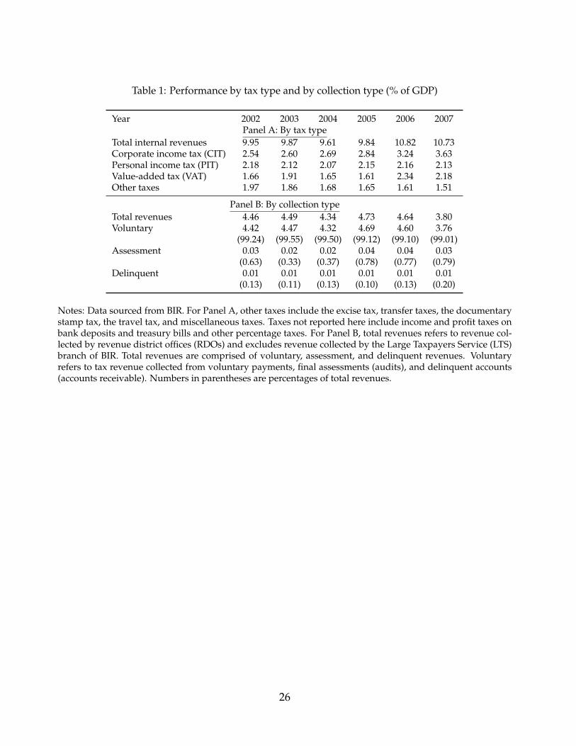
Table 1: Performance by tax type and by collection type (% of GDP)

Year 2002 2003 2004 2005 2006 2007Panel A: By tax type

Total internal revenues 9.95 9.87 9.61 9.84 10.82 10.73Corporate income tax (CIT) 2.54 2.60 2.69 2.84 3.24 3.63Personal income tax (PIT) 2.18 2.12 2.07 2.15 2.16 2.13Value-added tax (VAT) 1.66 1.91 1.65 1.61 2.34 2.18Other taxes 1.97 1.86 1.68 1.65 1.61 1.51

Panel B: By collection typeTotal revenues 4.46 4.49 4.34 4.73 4.64 3.80Voluntary 4.42 4.47 4.32 4.69 4.60 3.76

(99.24) (99.55) (99.50) (99.12) (99.10) (99.01)Assessment 0.03 0.02 0.02 0.04 0.04 0.03

(0.63) (0.33) (0.37) (0.78) (0.77) (0.79)Delinquent 0.01 0.01 0.01 0.01 0.01 0.01

(0.13) (0.11) (0.13) (0.10) (0.13) (0.20)

Notes: Data sourced from BIR. For Panel A, other taxes include the excise tax, transfer taxes, the documentarystamp tax, the travel tax, and miscellaneous taxes. Taxes not reported here include income and profit taxes onbank deposits and treasury bills and other percentage taxes. For Panel B, total revenues refers to revenue col-lected by revenue district offices (RDOs) and excludes revenue collected by the Large Taxpayers Service (LTS)branch of BIR. Total revenues are comprised of voluntary, assessment, and delinquent revenues. Voluntaryrefers to tax revenue collected from voluntary payments, final assessments (audits), and delinquent accounts(accounts receivable). Numbers in parentheses are percentages of total revenues.

26

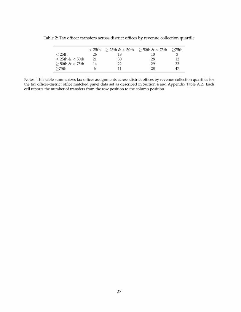
Table 2: Tax officer transfers across district offices by revenue collection quartile

< 25th ≥ 25th & < 50th ≥ 50th & < 75th ≥75th< 25th 26 18 10 3≥ 25th & < 50th 21 30 28 12≥ 50th & < 75th 14 22 29 32≥75th 6 11 28 47

Notes: This table summarizes tax officer assignments across district offices by revenue collection quartiles forthe tax officer-district office matched panel data set as described in Section 4 and Appendix Table A.2. Eachcell reports the number of transfers from the row position to the column position.

27

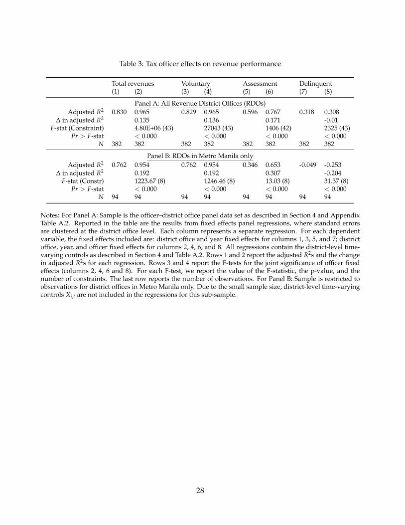
Table 3: Tax officer effects on revenue performance

Total revenues Voluntary Assessment Delinquent(1) (2) (3) (4) (5) (6) (7) (8)

Panel A: All Revenue District Offices (RDOs)Adjusted R2 0.830 0.965 0.829 0.965 0.596 0.767 0.318 0.308

∆ in adjusted R2 0.135 0.136 0.171 -0.01F-stat (Constraint) 4.80E+06 (43) 27043 (43) 1406 (42) 2325 (43)

Pr > F-stat < 0.000 < 0.000 < 0.000 < 0.000N 382 382 382 382 382 382 382 382

Panel B: RDOs in Metro Manila onlyAdjusted R2 0.762 0.954 0.762 0.954 0.346 0.653 -0.049 -0.253

∆ in adjusted R2 0.192 0.192 0.307 -0.204F-stat (Constr) 1223.67 (8) 1246.46 (8) 13.03 (8) 31.37 (8)

Pr > F-stat < 0.000 < 0.000 < 0.000 < 0.000N 94 94 94 94 94 94 94 94

Notes: For Panel A: Sample is the officer–district office panel data set as described in Section 4 and AppendixTable A.2. Reported in the table are the results from fixed effects panel regressions, where standard errorsare clustered at the district office level. Each column represents a separate regression. For each dependentvariable, the fixed effects included are: district office and year fixed effects for columns 1, 3, 5, and 7; districtoffice, year, and officer fixed effects for columns 2, 4, 6, and 8. All regressions contain the district-level time-varying controls as described in Section 4 and Table A.2. Rows 1 and 2 report the adjusted R2s and the changein adjusted R2s for each regression. Rows 3 and 4 report the F-tests for the joint significance of officer fixedeffects (columns 2, 4, 6 and 8). For each F-test, we report the value of the F-statistic, the p-value, and thenumber of constraints. The last row reports the number of observations. For Panel B: Sample is restricted toobservations for district offices in Metro Manila only. Due to the small sample size, district-level time-varyingcontrols Xi,t are not included in the regressions for this sub-sample.

28

Table 4: Placebo test for active influence of tax officers

All RDOs RDOs in Metro Manila(1) (2)

Total revenues 0.004 0.622(0.014) (0.692)[0.000] [0.017]

Voluntary 0.006 0.627(0.015) (0.702)[0.000] [0.017]

Assessment -0.062 0.044(0.161) (0.119)[0.004] [0.003]

Delinquent -0.071 -0.62(0.047) (0.157)[0.005] [0.014]

Notes: Sample is the collapsed officer–district office assignment spell panel data set as described in Subsection6.2. Each entry in this table corresponds to a different regression. In each column, we regress a placebo averageresidual in the second district office in years immediately prior to this officer actually being assigned to thatoffice (when a different officer was actually assigned) on the true average residual in the first assignment. SeeSubsection 6.4 for details. The first number in each cell is the estimated coefficient on the first assignmentresidual, the second number is the estimated standard error (in parentheses), and the third number is theestimated R2 (in square brackets). Column 1 includes all sample observations. Column 2 restricts the sampleto district offices in Metro Manila only.

29

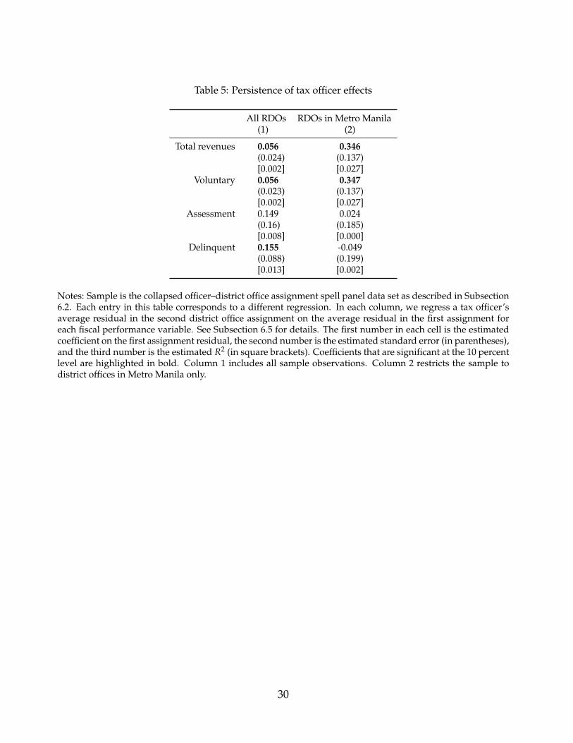
Table 5: Persistence of tax officer effects

All RDOs RDOs in Metro Manila(1) (2)

Total revenues 0.056 0.346(0.024) (0.137)[0.002] [0.027]

Voluntary 0.056 0.347(0.023) (0.137)[0.002] [0.027]

Assessment 0.149 0.024(0.16) (0.185)[0.008] [0.000]

Delinquent 0.155 -0.049(0.088) (0.199)[0.013] [0.002]

Notes: Sample is the collapsed officer–district office assignment spell panel data set as described in Subsection6.2. Each entry in this table corresponds to a different regression. In each column, we regress a tax officer’saverage residual in the second district office assignment on the average residual in the first assignment foreach fiscal performance variable. See Subsection 6.5 for details. The first number in each cell is the estimatedcoefficient on the first assignment residual, the second number is the estimated standard error (in parentheses),and the third number is the estimated R2 (in square brackets). Coefficients that are significant at the 10 percentlevel are highlighted in bold. Column 1 includes all sample observations. Column 2 restricts the sample todistrict offices in Metro Manila only.

30

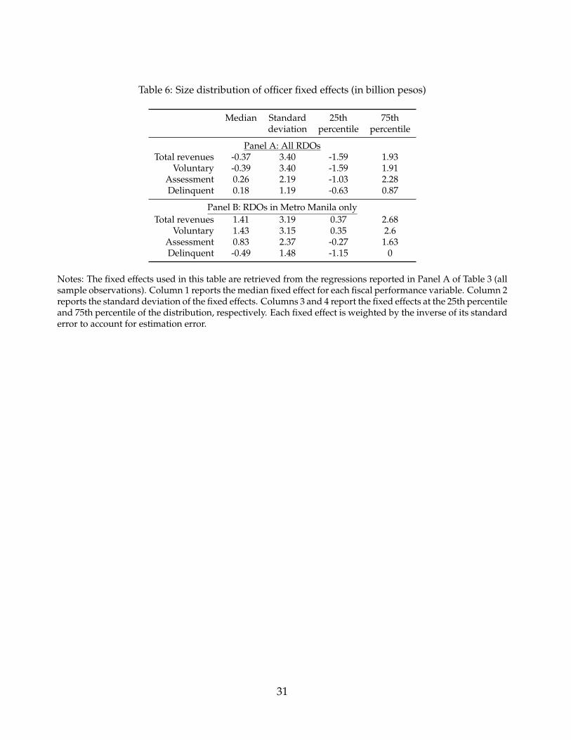
Table 6: Size distribution of officer fixed effects (in billion pesos)

Median Standard 25th 75thdeviation percentile percentile

Panel A: All RDOsTotal revenues -0.37 3.40 -1.59 1.93

Voluntary -0.39 3.40 -1.59 1.91Assessment 0.26 2.19 -1.03 2.28Delinquent 0.18 1.19 -0.63 0.87

Panel B: RDOs in Metro Manila onlyTotal revenues 1.41 3.19 0.37 2.68

Voluntary 1.43 3.15 0.35 2.6Assessment 0.83 2.37 -0.27 1.63Delinquent -0.49 1.48 -1.15 0

Notes: The fixed effects used in this table are retrieved from the regressions reported in Panel A of Table 3 (allsample observations). Column 1 reports the median fixed effect for each fiscal performance variable. Column 2reports the standard deviation of the fixed effects. Columns 3 and 4 report the fixed effects at the 25th percentileand 75th percentile of the distribution, respectively. Each fixed effect is weighted by the inverse of its standarderror to account for estimation error.

31

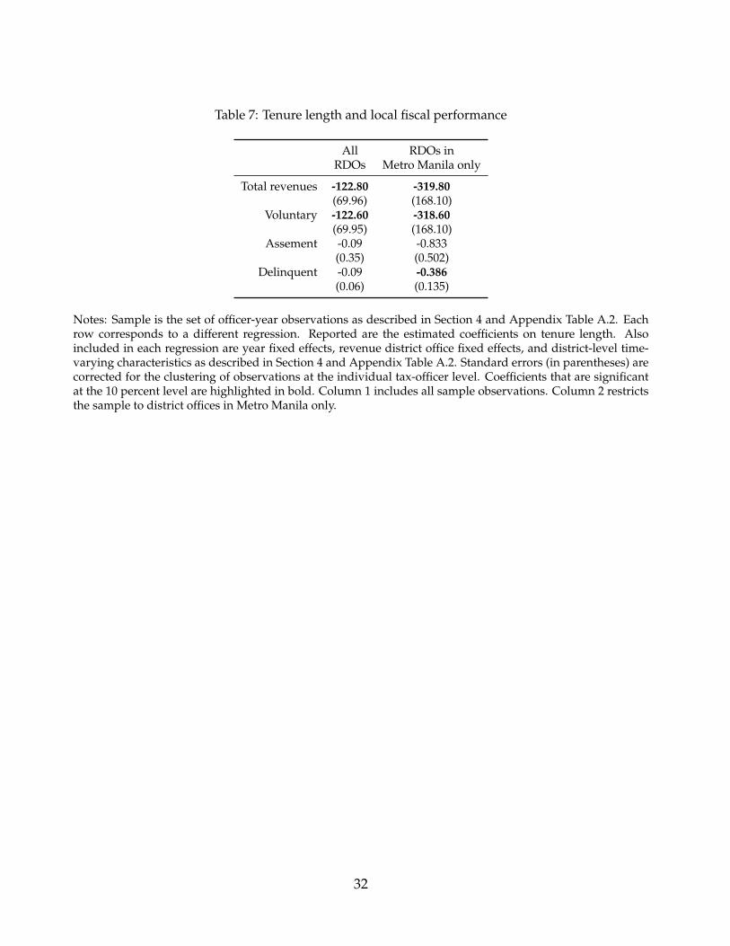
Table 7: Tenure length and local fiscal performance

All RDOs inRDOs Metro Manila only

Total revenues -122.80 -319.80(69.96) (168.10)

Voluntary -122.60 -318.60(69.95) (168.10)

Assement -0.09 -0.833(0.35) (0.502)

Delinquent -0.09 -0.386(0.06) (0.135)

Notes: Sample is the set of officer-year observations as described in Section 4 and Appendix Table A.2. Eachrow corresponds to a different regression. Reported are the estimated coefficients on tenure length. Alsoincluded in each regression are year fixed effects, revenue district office fixed effects, and district-level time-varying characteristics as described in Section 4 and Appendix Table A.2. Standard errors (in parentheses) arecorrected for the clustering of observations at the individual tax-officer level. Coefficients that are significantat the 10 percent level are highlighted in bold. Column 1 includes all sample observations. Column 2 restrictsthe sample to district offices in Metro Manila only.

32

Table 8: Revenue district office tax takes and tax officer fixed effects

All RDOs RDOs in Metro Manila(1) (2)

Total revenues 0.000342 0.000616(0.000194) (0.000299)

Voluntary 0.000344 0.000618(0.000195) (0.000300)

Assessment 0.0847 0.0543(0.0482) (0.0518)

Delinquent 0.0233 -0.376(0.0893) (0.132)

Notes: Each entry in this table corresponds to a different regression. The dependent variable in each regressionis the tax officer fixed effect on the row variable as retrieved from the regressions reported in Table 3. The inde-pendent variable is the average district office tax take for the district office in which we observe the tax officer.Reported are the estimated coefficients. Standard errors are in parentheses. Each observation is weighted bythe inverse of the standard error of the dependent variable. Coefficients that are significant at the 10 percentlevel are highlighted in bold. Column 1 includes all sample observations. Column 2 restricts the sample todistrict offices in Metro Manila only.

33

Online Appendix

Table A.1: Tax officer transfers across district offices by region

I CAR II III NCR IV-A IV-B V VI VII NIR VIII IX X XI XII ARMM XIIII 13 1 1 4 10 2 1 1 1CAR 8 2 2 1 1II 1 9 4 1III 10 12 1 3 1NCR 47 17 2 1 4 3 1 1 1 3 1IV-A 13 2 3 1 1 1IV-B 1 2 2 1V 14 1VI 1 10 4 4VII 11 4 1 1 1 3NIR 2 3VIII 14 1IX 8 3 2 1X 10 1 3 2XI 3XII 6 2ARMM 2 1 5 5XIII 1 1 10

Notes: This table summarizes tax officer assignments across district offices by region for the tax officer-district matched panel data set asdescribed in Section 4 and Appendix Table A.2. Regions are listed by geographical proximity (e.g., region CAR is contiguous to regions Iand II on the main island of Luzon). Each cell reports the number of transfers from the row position to the column position.

A1

Table A.2: Descriptive statistics

Mean Standard Min 25th 75th Maxdeviation percentile percentile

Panel A: Officer-level observable characteristicsNo. of transfers 1.75 0.60 1.00 1.00 2.00 4.00

Avg. length of assignment spell 3.07 1.70 1.00 2.00 4.00 12.00Work experience at BIR since 1989 6.24 3.94 1.00 3.25 9.00 19.00

Panel B: District-level fiscal outcomes (annual)All revenue district offices (RDOs)

Total revenues 1993.84 4545.58 16.69 225.17 1768.76 58620.63Voluntary 1978.54 4541.86 16.55 222.39 1756.57 58620.63

Assessment 12.64 25.10 0.00 0.12 12.62 230.34Delinquent 2.66 7.00 0.00 0.14 2.36 106.89

RDOs in Metro Manila onlyTotal revenues 6977.05 9274.57 1021.67 1751.58 7545.37 58620.63

Voluntary 6952.15 9277.87 1000.85 1743.31 7439.95 58620.63Assessment 20.79 28.13 0.00 0.06 31.45 144.32Delinquent 4.12 8.01 0.00 0.06 5.12 65.15

Panel C: District-level time-varying characteristics (annual)No. of officer turnovers 1.29 0.51 1 1 2 4

Internal revenue allotment (IRA) 847 638 0 430 1100 5470Constituency development funds (CDF) 458 621 0 0 763 3360

Local government expendituresGeneral public services 644 675 0 288 722 4630

Education, culture, sports 131 251 0 8 122 1450Health, nutrition 108 100 0 47 135 601

Labor, employment 1 3 0 0 1 33Housing, community development 3 8 0 0 24 97

Social security services 34 31 0 15 42 292Economic services 201 201 0 70 245 1270

Debt service 52 118 0 0 43 841Other 233 260 0 87 282 2760

No. of district-year observations (N) = 688No. of tax officers = 190

No. of district offices = 115

Notes: Sample includes all observations for years 2002-2007 for district offices which have tax officers that we do not observe in multipledistrict offices per year. The fiscal performance outcomes, IRA, CDF, and local government expenditures are in P millions. Work experienceat BIR and average length of assignment spell are in years.

A2

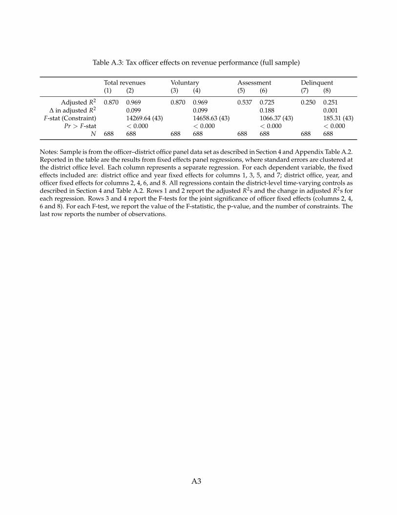
Table A.3: Tax officer effects on revenue performance (full sample)

Total revenues Voluntary Assessment Delinquent(1) (2) (3) (4) (5) (6) (7) (8)

Adjusted R2 0.870 0.969 0.870 0.969 0.537 0.725 0.250 0.251∆ in adjusted R2 0.099 0.099 0.188 0.001

F-stat (Constraint) 14269.64 (43) 14658.63 (43) 1066.37 (43) 185.31 (43)Pr > F-stat < 0.000 < 0.000 < 0.000 < 0.000

N 688 688 688 688 688 688 688 688

Notes: Sample is from the officer–district office panel data set as described in Section 4 and Appendix Table A.2.Reported in the table are the results from fixed effects panel regressions, where standard errors are clustered atthe district office level. Each column represents a separate regression. For each dependent variable, the fixedeffects included are: district office and year fixed effects for columns 1, 3, 5, and 7; district office, year, andofficer fixed effects for columns 2, 4, 6, and 8. All regressions contain the district-level time-varying controls asdescribed in Section 4 and Table A.2. Rows 1 and 2 report the adjusted R2s and the change in adjusted R2s foreach regression. Rows 3 and 4 report the F-tests for the joint significance of officer fixed effects (columns 2, 4,6 and 8). For each F-test, we report the value of the F-statistic, the p-value, and the number of constraints. Thelast row reports the number of observations.

A3

Table A.4: Tax officer effects on revenue performance (controlling for regional time trends)

Total revenues Voluntary Assessment Delinquent(1) (2) (3) (4) (5) (6) (7) (8)

Adjusted R2 0.828 0.962 0.828 0.962 0.584 0.756 0.311 0.308∆ in adjusted R2 0.134 0.134 0.172 -0.003

F-stat (Constraint) 2256.16 (31) 113.36 (31) 175.06 (31) 11.33 (31)Pr > F-stat < 0.000 < 0.000 < 0.000 < 0.000

N 382 382 382 382 382 382 382 382

Notes: Sample is from the officer–district office panel data set as described in Section 4 and Appendix Table A.2.Reported in the table are the results from fixed effects panel regressions, where standard errors are clustered atthe district office level. Each column represents a separate regression. For each dependent variable, the fixedeffects included are: district office and year fixed effects for columns 1, 3, 5, and 7; district office, year, andofficer fixed effects for columns 2, 4, 6, and 8. Rows 1 and 2 report the adjusted R2s and the change in adjustedR2s for each regression. The last row reports the number of observations.

A4

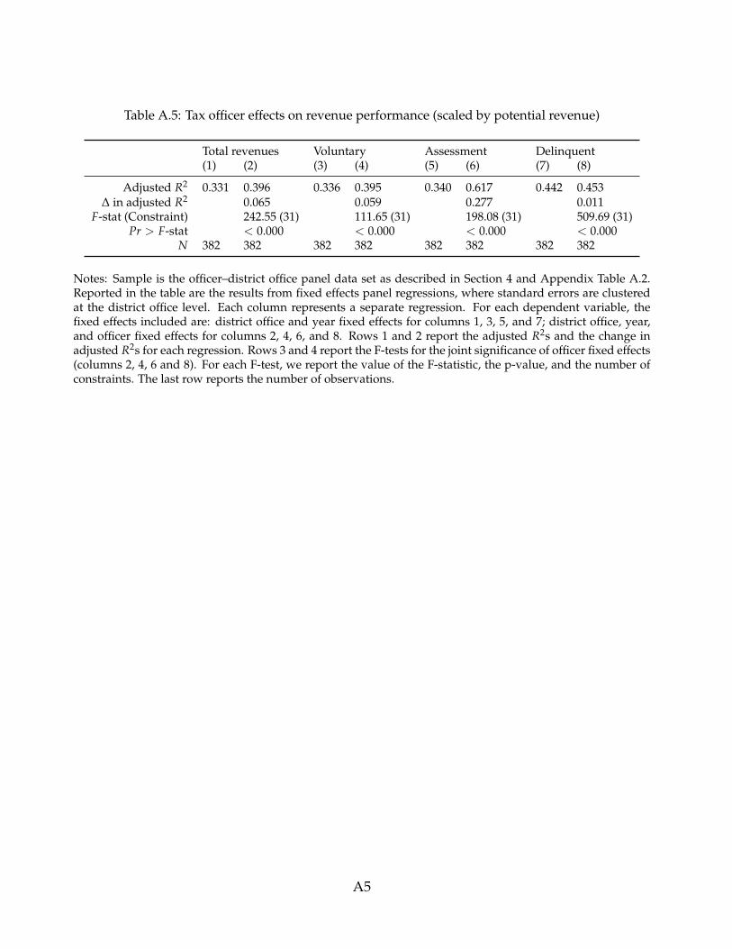
Table A.5: Tax officer effects on revenue performance (scaled by potential revenue)

Total revenues Voluntary Assessment Delinquent(1) (2) (3) (4) (5) (6) (7) (8)

Adjusted R2 0.331 0.396 0.336 0.395 0.340 0.617 0.442 0.453∆ in adjusted R2 0.065 0.059 0.277 0.011

F-stat (Constraint) 242.55 (31) 111.65 (31) 198.08 (31) 509.69 (31)Pr > F-stat < 0.000 < 0.000 < 0.000 < 0.000

N 382 382 382 382 382 382 382 382

Notes: Sample is the officer–district office panel data set as described in Section 4 and Appendix Table A.2.Reported in the table are the results from fixed effects panel regressions, where standard errors are clusteredat the district office level. Each column represents a separate regression. For each dependent variable, thefixed effects included are: district office and year fixed effects for columns 1, 3, 5, and 7; district office, year,and officer fixed effects for columns 2, 4, 6, and 8. Rows 1 and 2 report the adjusted R2s and the change inadjusted R2s for each regression. Rows 3 and 4 report the F-tests for the joint significance of officer fixed effects(columns 2, 4, 6 and 8). For each F-test, we report the value of the F-statistic, the p-value, and the number ofconstraints. The last row reports the number of observations.

A5

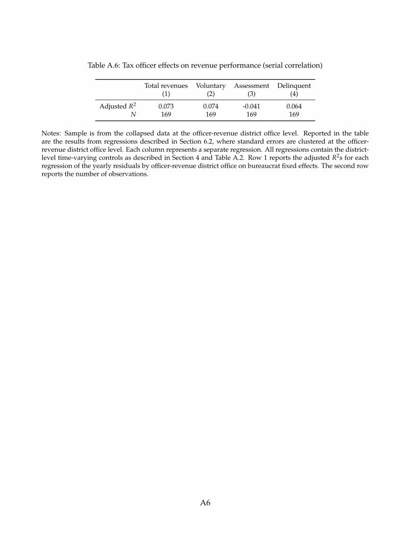
Table A.6: Tax officer effects on revenue performance (serial correlation)

Total revenues Voluntary Assessment Delinquent(1) (2) (3) (4)

Adjusted R2 0.073 0.074 -0.041 0.064N 169 169 169 169

Notes: Sample is from the collapsed data at the officer-revenue district office level. Reported in the tableare the results from regressions described in Section 6.2, where standard errors are clustered at the officer-revenue district office level. Each column represents a separate regression. All regressions contain the district-level time-varying controls as described in Section 4 and Table A.2. Row 1 reports the adjusted R2s for eachregression of the yearly residuals by officer-revenue district office on bureaucrat fixed effects. The second rowreports the number of observations.

A6

Figure A.1: Revenue Travel Assignment Order (RTAO) Example

A7