Do Currency Unions Deliver More Economic

Integration than Fixed Exchange Rates?

Evidence from the CFA and the ECCU

David Fielding* and Kalvinder Shields**

March 2003

Address for correspondence (until August 2003):

UNU/WIDER, Katajanokanlaituri 6B

00160 Helsinki, Finland

E-mail: fielding@wider.unu.edu

Telephone: +358-9-615-99225

Abstract

In this paper we develop a model to identify determinants of macroeconomic integration in the

African CFA Franc Zone and in Dollar-pegging Caribbean countries (including members of the

East Caribbean Currency Union). These two groups of countries each comprise states using several

different local currencies: on the one hand the BCEAO-CFA Franc and the BEAC-CFA Franc (both

pegged to the Euro), on the other the ECCU Dollar and other national Dollar-pegged currencies.

The purpose of the analysis is to distinguish the effect of monetary union on macroeconomic

integration from the effect of pegging to a common OECD currency.

Keywords: Currency Unions, International Integration

JEL Classification: F15, F33

* Department of Economics, University of Leicester and WIDER, United Nations University, Helsinki. ** Department of Economics University of Melbourne.

1

Do Currency Unions Deliver More Economic Integration than Fixed Exchange Rates?

Evidence from the CFA and the ECCU

1. Introduction

Over the last decade, many countries have chosen to adopt “hard” exchange rate pegs, or to become

part of an international monetary union (Ghosh et al., 1995). These changes have renewed academic

interest in the impact of the exchange rate regime and monetary union on international

macroeconomic integration. Papers such as Artis and Zhang (1995), Christodoulakis et al. (1995),

Fatas (1996) and Boone (1997) examine the impact of exchange rate pegs on the magnitude of

business cycle correlations. These studies on the magnitude of the correlation of shocks run parallel

to a literature on the impact of exchange rate regimes on the persistence of asymmetric shocks, and

in particular on the persistence of deviations from PPP (for example, Lothian and Taylor, 1996,

Papell, 1997 and Engel and Rogers, 2001). Evidence on the impact of complete monetary union is

necessarily more limited – given the small number of countries that have adhered to a monetary

union for any length of time – but Rose and Engel (2000) look at their impact on business cycle

correlations and trade.

Overall, there appears to be some evidence to confirm the conjecture (as in for example

Obstfeld and Rogoff, 1996) that sharing a common currency, or alternatively adopting a hard

exchange rate peg with one’s main trading partner, reduces international transactions costs and

exchange rate risk, which promotes greater trade and hence also greater business cycle

synchronicity. It also appears to insulate partner countries from speculative bubbles that lead to

temporary and unnecessary fluctuations in the real exchange rate. However, there is some

disagreement about the robustness of these results, as exemplified by the debate between Rose

(2001) and Persson (2001). One worry is that evidence based on linear regression equations that

incorporate an exchange rate regime dummy might suffer from bias because such equations do not

adequately capture nonlinearities in the process determining the level of integration.

Whatever the strength of the results published so far, none of these papers directly addresses

the question of whether the impact of full monetary union on macroeconomic integration differs

from that of adopting a hard peg. This is of potential policy importance, because for some countries

the administrative or political costs of joining a monetary union may be prohibitively high. If

adopting a hard peg is a close macroeconomic substitute to complete monetary integration, the

benefits of such integration are likely to be available to a wider range of nation states.

Indeed, existing empirical papers provide very ambiguous evidence about the role of hard

pegs versus the role of currency unions. Apart of the Europe-specific papers (none of which

provides direct evidence on the impact of full monetary union, given the short time the EMU has

2

been in existence), a substantial part of the international evidence relies on the inclusion of

observations from the world’s two long-lasting trans-national common currency areas: the CFA

Franc Zone in Africa and the East Caribbean Currency Union (ECCU). In panel and cross-section

studies, these areas provide the bulk of observations for both fixed exchange rate regimes and

monetary unions.1

Using these currency areas as the basis for empirical evidence leaves to one side a

potentially important point. The integration benefits to a small open economy from adhering to a

currency union might arise not so much from the shared currency as from the common peg. So, for

example, the increased integration between Puerto Rico and the Bahamas resulting from their

dollarization, or between St. Lucia and Dominica resulting from their common use of the ECCU

Dollar (which is pegged to the US Dollar), may be no greater than their integration with Barbados

(which maintains a conventional peg against the US Dollar). The existing results from francophone

countries are even more ambiguous. Typically, the CFA has been treated as a single currency union,

when in fact it comprises two quite separate currencies, each issued by a different central bank and

separately pegged to the French Franc (and now to the Euro). So, for example, Togo and Gabon (in

different currency areas within the CFA) have been treated as members of the same currency union,

but Togo and Mayotte (which uses the French Franc) have not. In fact, all three countries use

different currencies, each exchangeable with the others at a fixed rate.

This paper will address these ambiguities by looking at the degree of macroeconomic

integration between countries in two areas of the world. First, we will examine pair-wise measures

of integration between the nations of the CFA, all of which use one currency or another called the

CFA Franc and pegged to the French Franc / Euro. Some of the pairs are made up of economies

within the same monetary union, and others are cross-union pairings. Second, we will look at the

same measures for a group of Caribbean countries, all of which use currencies pegged to the US

Dollar. Some are members of the ECCU, some have dollarized national currencies and others

maintain conventional independent pegs.

The purpose of the comparisons is to see whether adhering to a common currency delivers a

degree of integration over-and-above that resulting from adherence to a common peg. Some of the

theoretical explanations for greater integration are based on currency transactions costs, and suggest

that integration arises from full monetary union, rather than from a common peg. Others are based

on exchange rate volatility and exchange risk, and suggest that (credible) adherence to a common

peg might suffice.2

1 For example, the data set employed by Rose and Engel (2000) includes 256 pairs of countries identified as sharing a currency, of which 120 are CFA or ECCU pairs. A further 116 are US Dollar or French Franc pairs. 2 Even if the marginal effect of a common currency over a common peg is negligible, some countries might be able to adhere credibly to a peg only within a monetary union, because of the political fragility of domestic monetary

3

The next section provides a brief, non-technical survey of the possible reasons why

monetary union might affect the degree of international economic integration. We will focus on

three aspects of integration: trade intensity, the magnitude relative price volatility, or of deviations

from PPP, and the degree of business cycle synchronization. Section 3 introduces the countries that

will appear in our analysis. Section 4 then discusses the econometric framework that will be used in

Section 5 to measure the degree of integration. The aim is to build a modelling framework based on

realistic assumptions about the structure of the small open economies that form our sample, a

structure rather different than that of the typical OECD economy.

2. Monetary Union and Economic Integration

The existing literature suggests at least three aspects of international economic integration that

could in principle be affected by membership of a monetary union as opposed to a fixed exchange

rate.

(i) The use of a common currency will eliminate transactions costs in international trade

(De Grauwe, 2000), so trade volumes ought to increase. For one of the two regions we

will be examining – the ECCU – this aspect of integration is not really relevant. Most of

the Caribbean countries specialize in tourism and (to a lesser extent) cash crop

production: areas in which there is little scope for intra-regional trade. Trade within the

region makes up less than 10% of the total trade volume. For the CFA, however, intra-

regional trade is much more important. Trade between CFA countries and other LDCs

makes up a substantial fraction of the total trade volume (in some cases, more than 50%:

see Table 1).

(ii) Engel and Rogers (2001) identify a number of factors that determine the degree of real

exchange rate volatility between pairs of countries. Nominal exchange rate volatility and

physical distance turn out to be important factors, but there is also a substantial “pure”

border effect. Controlling for all other factors, the ratio of prices in two regions is more

volatile if the regions are located in different countries. Engel and Rogers suggest a

number of explanations for this effect. Some of these, including the currency

transactions costs mentioned above, but also factors such as international heterogeneity

institutions. So monetary union can still be a significant factor in international integration, even if the only economic consequences of monetary union are those arising from the common peg. The political economy of monetary union is, however, beyond the scope of this paper.

4

in marketing and distribution systems, the scope for international price discrimination, or

“informal” trade barriers, might be reduced if the countries shared a common currency.3

(iii) As a consequence of increased trade, the degree of business cycle synchronicity between

two countries in a monetary union might be higher, because aggregate demand shocks in

one country have more of an impact on the other than they would otherwise; or it might

be lower, because increased trade corresponds to increased specialization in types of

production subject to different productivity shocks. But an increased volume of bilateral

trade is not the only way in which a common currency could affect business cycle

synchronicity. For example, if multinational firms have less scope for price

discrimination between members of a monetary union (because price differences are

more transparent and because the elimination of currency transactions costs facilitates

arbitrage in goods), then international productivity shocks are likely to be passed on to

local markets in a more uniform way.

[Table 1 here]

In this paper we will use data from our two regions to assess the extent to which membership of the

same monetary union influences the degree of international macroeconomic integration, over and

above a fixed exchange rate effect. We will measure integration in terms of (i) trade volumes (in the

CFA only), (ii) real exchange rate volatility and (iii) business cycle synchronicity. The precise

measures used will be discussed in Section 4.

3. Monetary Union in Africa and the Caribbean

3.1 The CFA Franc Zone

The CFA evolved from the monetary institutions of the last phase of French colonial Africa. Figure 1

shows a map of the CFA region. It comprises two monetary areas, each with its own currency and

central bank: the West African Economic and Monetary Union (UEMOA), using currency issued by

the Central Bank of West African States (BCEAO); and the Central African Economic Area

(UDEAC), using currency issued by the Bank of Central African States (BEAC). Both currencies are

commonly called the CFA Franc, although they are entirely separate monetary units.

The countries that make up the CFA, and their basic economic structure, are summarised in

Tables 2-3. The boundaries between the different monetary areas have a geographical and historical

basis, and each of the two monetary unions (the BCEAO and BEAC regions) comprises a wide range

of economies. The BCEAO region includes both semi-industrialised economies with a high export-

3 For example, traders’ lives will be made easier if they only have to hold one type of currency with which to bribe customs officials.

5

GDP ratio (such as Cote d’Ivoire and Senegal) and also some of the world’s poorest and

underdeveloped countries (such as Burkina Faso and Mali). The BEAC region includes both countries

that are equally underdeveloped (Chad, Central African Republic and Equatorial Guinea) and

relatively high-income petroleum exporters (Cameroon, Congo Republic and Gabon).

Each of the two currencies is exchangeable for the French Franc at a rate of 100:1 (and now at

the equivalent Euro rate). The French Treasury is obliged to exchange CFA Francs for Euros at this

fixed rate,4 and there are rules limiting CFA government borrowing that are intended to prevent the

African countries from abusing France’s guarantee of convertibility. However, France is not part of

the CFA, and the only legal tender in each CFA country is the currency issued by its central bank.

Foreign currency (including the other CFA currency) is not used as a unit of account or medium of

exchange. Commercial banks do not typically offer customers foreign currency deposit facilities, and

foreign currency deposits are a negligibly small fraction of total deposits. The exchange of one CFA

currency for another (or of CFA Francs for Euros) must be conducted through the central bank and,

and is subject to taxation, so intra-CFA currency transactions costs are not negligible (Vizy, 1989).

[Figure 1 and Tables 2-3 here]

The composition of the two monetary unions is a consequence of the French colonial organisation,

and is therefore exogenous to contemporary economic characteristics. The current grouping into two

currency areas dates from 1955 (seven years before full political independence, at which point the

countries were self-governing French overseas territories), and arises from the distinction between

French West Africa and French Equatorial Africa in the colonial period. As can be seen from the map,

this division is based on the physical geography of the region. The only point of physical contact

between the UEMOA and the UDEAC is the Chad-Niger border, which lies in the Sahara Desert far

from any major centers of population. Further south, the two areas are separated by Nigeria, a former

British colony that has no part in the CFA. The CFA comprises those Sub-Saharan African countries

occupied by France at the end of WW1.5 There have been just two exits from the CFA, neither of

which is likely to have been correlated with the countries’ economic characteristics. In 1958, at the

institution of the Fifth French Republic, all overseas territories participated in a referendum on the

new constitution. Guinea-Conakry, which happened to have a socialist government at the time, was

the only colony to reject this constitution, and severed all political and financial links with France. In

1973, after full independence, Mauritania (the only Arab country in the area) also exited the CFA,

preferring to pursue an identity as a North African Arab state. There have also been just two entries:

Equatorial Guinea and Guinea-Bissau. These countries were, respectively, Spanish and Portugese

4 In effect, France pegs the Euro to the CFA currencies. Monetary policy in the CFA is constrained not by the need to maintain an exchange rate peg, but by (very lax) rules limiting domestic credit creation.

6

colonies; they are completely surrounded by, respectively, UDEAC and UEMOA nations, and joined

the appropriate monetary union in 1985 and 1997. The only other countries surrounded by the CFA

(Gambia, Ghana, Liberia, Nigeria and Sierra Leone) are all English-speaking. All but Liberia were

British colonies, and up until now it has been made clear that they are not welcome to join the

francophone monetary area.

In this paper we will focus on those 12 of the 14 members of the CFA for which adequate

macroeconomic data are available: Benin (designated ben in the tables), Cote d’Ivoire (civ), Mali

(mli), Niger (ner), Senegal (sen) and Togo (tgo) in the BCEAO area and Cameroon (cam), Central

African Republic (car), Chad (tcd), Congo Republic (cgo) and Gabon (gab) in the BEAC region.6 If

sharing a common currency delivers an additional degree of integration over-and-above that arising

from the common currency peg, then we should see a greater degree of integration within each of the

two monetary unions than we do across the BCEAO-BEAC border, conditional on other, exogenous

economic characteristics.

3.2 The ECCU and other Dollar-pegging Caribbean countries

The East Caribbean Currency Union is made up of eight island economies. Adequate data are

available for the analysis of macroeconomic shocks in six of these: Antigua and Barbuda (atg),

Dominica (dma), Grenada (grd), St. Kitts and Nevis (ktn), St. Lucia (lca) and St. Vincent and the

Grenadines (vct).7 As with the CFA, this currency union owes its existence to colonial history: the

member states formed Britain’s colonial possessions in the Eastern Caribbean. Spanish and French-

speaking islands are excluded. Members share a single central bank issuing the ECCU Dollar, pegged

to the US Dollar at a fixed rate. Proximity to the USA and a large amount of tourism mean that US

Dollars also circulate in these countries. However, the use of the ECCU Dollar as a unit of account

and as a medium of exchange by all of the (sizeable) public sectors institutions across the islands

ensures that the domestic private sector must deal largely in the local currency. In December 2000, for

example, private sector foreign currency deposits in the ECCU made up only 15.7% of total private

sector bank deposits. This is not significantly different from the equivalent figure for OECD

countries: the ratio for Great Britain in the same period was 13.3%.8 The ECCU-US$ exchange rate

has remained fixed for many years, but re-pegging is not impossible. Indeed, the currency was

originally pegged to UK Sterling. In this sense, membership of the ECCU does not entail a currency

union with the USA, and the ECCU countries are not dollarized.

5 Excepting Djibouti, which is thousands of miles away in the Horn of Africa. 6 The two countries lacking adequate data are Guinea-Bissau in the BCEAO region and Equatorial Guinea in the BEAC region. 7 The two other ECCU members are Aruba and Montserrat. 8 The figures come from the central bank websites: www.eccb-centralbank.org and bankofengland.co.uk.

7

Many other Caribbean countries have maintained a peg against the US Dollar at one time or

another. However, there are just two sizeable economies that have avoided a flexible exchange rate

regime from independence through to the 21st century: the Bahamas (bhs), and Barbados (brb), plus

two Central American economies: Belize (blz) and Panama (pan). In the case of the Bahamas and

Panama, the fact that the peg has been retained for so long is a result of geo-political factors,9 and the

two countries are completely dollarized, with no separate currency of their own. Barbados and Belize

have maintained conventional fixed pegs against the US Dollar. If sharing a common currency

delivers an additional degree of integration over-and-above that arising from the common currency

peg, then we should see a greater degree of integration within the ECCU than we do between ECCU

countries and the other four countries, conditional on other, exogenous economic characteristics.

Note that we will not be looking at the degree of integration between each of the small open

economies and the large economy issuing the anchor currency. Our econometric methodology is

based on the assumption that foreign prices are exogenous, an assumption valid only for a small open

economy.

4. Testing for the Marginal Effect of Adhering to a Common Currency

Our basic methodology is similar to that of Rose and Engel (2000), but with different dependent

variables and a different data set. The extent of macroeconomic integration between two countries

might depend on a variety of factors other than their currency institutions. So our approach is to

construct a fixed-effects regression for different measures of integration in any two countries i and j,

conditional on both a common currency dummy (ifsij) and a set of exogenous conditioning

variables.

In the empirical section that follows we will employ four different measures of integration.

The first is the total value of bilateral trade between two countries, in millions of dollars (Tij). This

corresponds to integration concept (i) in Section 2. Tij ought to be higher in countries sharing the

same currency. The second, in the spirit of Engel and Rogers (2001), is a measure of unconditional

real exchange rate volatility, that is, the standard deviation of the (log) ratio of annual consumer

price indices in i and j over the period for which data are available (Sij). This corresponds to

integration concept (ii) in Section 2. Sij ought to be lower in countries sharing the same currency.

However, one might question whether this unconditional measure of volatility is the most

appropriate for our purposes. In the short run (i.e., over a period shorter than that in which arbitrage

guarantees PPP), prices could vary in response to a wide variety of macroeconomic factors. For

example, in the CFA the two different central banks can each pursue an active monetary policy.

9 Panama shared a land border with the USA until the latter ceded the Canal Zone in 2000; the Bahamas are only a few miles from the coast of Florida.

8

Interest parity with France does not hold in the short run, and the differential between each central

bank’s base rate and that of the European Central Bank varies over time; so does the differential

between the interest rates in the two parts of the CFA. The Euro-CFA Franc peg is guaranteed by

the French Treasury, so short-run monetary policy in the CFA is not constrained by the need to

maintain the peg. Idiosyncratic innovations in monetary policy could generate price deviations. Two

countries in different currency areas might exhibit a large degree of unconditional real exchange

rate volatility not because using different currencies creates underlying structural asymmetries, but

just because the two monetary authorities are following different policies. Conditioning out the

monetary shocks might give a more informative indicator of the degree of underlying

macroeconomic integration.

So an alternative way of measuring the degree to which prices in two countries are tied

together is to estimate the size of annual price changes conditional on short-run factors like changes

in the money supply, and then to look at the extent of correlation between the price innovations in

two countries. In other words, we need a macro-econometric model incorporating a real exchange

rate equation. In the case of the CFA, such a model is provided by Fielding and Shields (2001), who

construct a structural VAR model that provides estimates of the innovations in domestic prices in CFA

countries, conditional on growth in output, money and foreign prices.10 We use these estimates for our

CFA sample; we also replicate the model with Caribbean country data. For the sake of brevity, we do

not discuss the model in detail here. Its econometric rationale is similar in spirit to that of Blanchard

and Quah (1989), but with a different underlying economic structure, based on assumptions that are

more realistic for a small open economy. We assume that in the long run, inflation rates in the each

country in the CFA will converge on French inflation,11 and inflation rates in each Caribbean

country on US inflation. However, short run movements in real output and in the money supply can

generate fluctuations in prices around the level consistent with PPP with OECD countries. In

addition to these fluctuations, there are also short-run innovations in domestic prices, estimated as

forecast errors in the model. If sharing a common currency ties countries’ prices together more

closely than does a fixed exchange rate (conditional on money and output shocks), then these

innovations should be more closely correlated between members of a monetary union than they are

between countries that just happen to peg to the same OECD currency. The innovation correlation

coefficient, ijp, is our third measure of integration.

The econometric model is also used to construct the fourth measure of integration: the

degree of business cycle synchronicity, corresponding to concept (iii) in Section 2. Here we are

concerned with the measurement of the extent to which aggregate supply and aggregate demand

10 However, this paper does not explore the factors that might explain the cross-country correlations in price innovations.

9

shocks in one country are passed on to another. Again, we wish to condition on monetary policy: in

the long run, money is neutral, but in the short run money shocks can impact on output. So the

output shocks are measured as innovations in the output equation in the model. The correlation

coefficient for this second type of innovation, ijy, is our fourth measure of integration.

5. Empirical Results

This section is divided into three parts. The first presents the results of estimating equation (1) using

the trade intensity measure of integration (measure i in Section 2); the second presents the results of

using unconditional real exchange rate volatility (measure ii); the third presents the results of using the

estimated price and output innovation correlations (measures iii and iv).

We have two samples for use with the four alternative dependent variables. The first is made

up of the 66 country pairs among the 12 CFA countries. The second is made up of the 45 country

pairs among 10 Caribbean and Central American countries. In the CFA sample, ifsij = 1 in 31 cases

(when both countries are in the BCEAO area, or both are in the BEAC area); in the Caribbean

sample, ifsij = 1 in 15 cases (when both countries are ECCU members). The data used to construct

the conditioning variable (i-iv in Section 3) are taken from the World Bank World Development

Indicators.

5.1 The impact of a common currency on trade intensity

In this case, we present results only for the CFA sample, since the volume of trade among the

Caribbean countries is a very small fraction of their total trade. The regression for trade intensity is

based on an equation of the form:

ijijijjiij uXifsDDfT ),,,()1ln( (1)

uij is a residual, and Xij a vector of conditioning variables. Di is a dummy variable for the ith country.

It turns out that country-specific effects have a large part to play in predicting trade intensity, and it

might not necessarily be the case that the economic characteristics contained in the X-vector fully

capture these effects. In other words, we will allow for unobserved country-specific characteristics

to affect Tij. These characteristics might incorporate a range of factors. For example, Rose and van

Wincoop (2001) and Anderson and van Wincoop (2001) suggest that it is important to take account

of the magnitude of each country’s barriers to trade with all its trading partners, a factor difficult to

measure in our sample of countries with very limited fiscal data.

11 Evidence for this is cited in Fielding and Shields (2001).

10

The X-vector comprises a number of economic characteristics. To the extent that integration

is a function of the volume of bilateral trade flows, the explanatory variables in “gravity” models of

international trade will enter into X:

(i) The log-product of the two countries’ total initial GDP (in US Dollars): yi·yj

(ii) The log-product of their initial per capita GDP (in US Dollars): yPi·yP

j

(iii) The log-product of their land surface areas (in km2): ai·aj

(iv) A dummy variable for whether the countries share a land border: ifbij

(v) The logarithm of the Great Circle distance between their capital cities (in radians): distij

(vi) A dummy variable for whether the two countries have a maritime coastline: ifcij

Figures for (i-iii) are taken from the World Bank World Development Indicators. However, these

conditioning variables might also affect the magnitude of macroeconomic integration for other

reasons. For example, larger or more developed countries might be less susceptible to speculative

behavior that induces unanticipated deviations in the real exchange rate; so real exchange rate

volatility might be lower. In this paper, we do not attempt to identify the channels through which

the conditioning variables impact on our macroeconomic integration measures.

The ifsij dummy appears in equation (1) in order to capture the possibility that sharing a

common currency (rather than just having a fixed exchange rate) reduces transactions costs in

international trade, as outlined in section 2 above. In this sense, it has a role similar to the variables

in the equation reflecting the determinants of international transport costs: ifbij, distij and ifcij. A

simple version of equation (1) might treat the four cost variables as linearly separable arguments of

f(). However, in the light of comments by, for example, Persson (2001), the linearity assumption is

questionable. The magnitude of the impact of a common currency on trade between two countries

could depend on the size of transport costs, if only because larger transport costs could increase the

size of the currency transactions involved, ceteris paribus. But also, the magnitude of informal

barriers to trade might depend on the two elements of costs – for transport and for currency

transactions – in a more complex way. For this reason, a more appropriate form of equation (1) will

include terms interacting ifsij with the other cost variables:

ijijijijij

ijijijijjiPj

Pijijjiiij

uifcifsdistifs

ifcdistifbifsaayyyyDDT

][][)1ln(

21

4321321 (1a)

where ijij ifcifs = 1 if either ijifs = 1 or if ijifc = 1 and zero else. ifsij is not interacted with ifbij

because there is only one case of a land border between a UEMOA country and a UDEAC country

11

(Niger and Chad). Of course, we do not know a priori whether we have successfully captured all

the relevant non-linearities in this way. So testing the validity of this functional form will be an

important part of the econometric exercise.

[Tables 4-5 here]

The regression results are presented in Table 4. For each explanatory variable, the estimated

coefficient is reported alongside the corresponding standard error (using White’s correction for

heteroskedasticity), “h.c.s.e.”, the resulting t-ratio and the corresponding partial R2. In these

regressions the Tij figures used are taken from IMF DOTS for 1997. The table includes two

regression equations. The first is the unrestricted equation (1a); the second is a more parsimonious

form in which some conditioning variable coefficients have been set to zero so as to minimize the

Akaike Criterion. (This criterion, AIC, along with the Schwartz and Hannon-Quinn Criteria, SC and

HC, is reported at the bottom of the table.) Those coefficients that are statistically significant in the

unrestricted equation do not change substantially in the restricted one, so we are reasonably

confident that our inferences are robust to the inclusion of nuisance parameters in the model. Table

5 includes a test for the validity of the functional form that we have chosen. This is a Ramsey

RESET test for adding powers of the fitted residuals up to the fourth order to the regression

equation. In neither the unrestricted nor the restricted version of the equation can we reject the null

that the functional form we have chosen is an adequate description of the data.

The table shows that the most important factor explaining trade intensity, aside from country

fixed effects, is whether two countries share a land border. The point estimate in the unrestricted

equation is 1.53. That is, countries sharing a land border have a volume of trade that is over 150%

higher than trade with more distant countries, ceteris paribus. There is also a negative coefficient on

the distance variable (-0.68), and a positive coefficient on the per capita income variable (0.61),

although these become statistically significant only in the restricted equation.

Finally, there is a positive coefficient on the interaction term ijij ifcifs that is significantly

different from zero, but not from unity. In other words, if two countries either both have a coastline

or both share the same currency, their trade volume is about twice as high as otherwise. Neither ifsij

alone nor ifcij alone has a significant impact on trade. One interpretation of this effect is that using a

different currency is a substantial barrier to trade in landlocked countries only. Landlocked

countries rely on their maritime neighbours – neighbours in the same currency area – for the

transportation of imports and exports. The inland countries generally face higher transport costs. It

seems that the combination of currency transaction costs and relatively high transport costs is

enough to inhibit trade, but either of these two effects alone is not in itself large enough to have a

12

significant impact on trade volumes. In other words, the benefit of sharing a single currency, over

and above any benefit of a fixed exchange rate, depends on geographical location.

5.2 The impact of a common currency on unconditional real exchange rate volatility

In this section we discuss the results of the corresponding regression equations for the real exchange

rate volatility measure, Sij. For this measure of integration, we require a different regression equation

with different conditioning variables. The degree of variation in relative prices across two countries is

likely to depend on the degree of heterogeneity in their production structures, and the degree of

correlation in the external price shocks that they face. It might also depend on their geographical

proximity, if variations in local prices depend on variations in local climate, or if the strength of

international commodity arbitrage in the short run depends on transportation costs between markets. So

our regression equation is of the form:

ijijijijij

ijjijijjiiij

uifsifcdistifb

ctotfddfggfDDS

4321

321 )(|)(||)(| (2)

Sij is measured as a standard deviation using the time-series price data described in Section 5.3. gi is the

ratio of agricultural value added to GDP in country i, di is the ratio of industrial value added to GDP,

and the transformation f(x) = log(1+x) – log(1-x) ensures that the explanatory variables are

approximately normally distributed. ctotij is the correlation of the terms of trade in country i with that

in country j. All figures are based on annual data for 1970-1999 from the World Bank World

Development Indicators. In the light of the discussion in section 2 above, it is also conceivable that Sij

will depend on Tij; however, the trade variable was never statistically significant in IV estimates of

equation (2). Again, it will be important to test for the validity of this functional form.

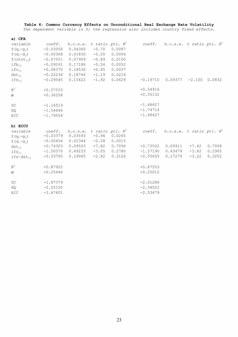
[Table 6 here]

Table 6 reports the regression results using Sij as the dependent variable. The first half of the table

relates to the regression equation for the CFA zone; the second half relates to the regression equation

for the ECCU and its neighbors. The table shows that in the first case (the CFA), the only significant

factors (other than fixed effects) is the monetary union dummy ifsij. The estimated coefficient on the

monetary union dummy is –0.3, so countries sharing the same currency can be expected to have a

standard deviation of relative prices that is about 30% lower, ceteris paribus. The RESET test statistics

in Table 5 indicate that there are no substantial non-linearities biasing these results: the size of the

monetary union effect does not depend on other economic characteristics.

The same cannot be said for the ECCU sample. When a regression taking the form of equation

(2) was fitted to the Caribbean data, the RESET test statistics was greater than the 5% critical value.

13

The reason for this is that in the Caribbean the size of the single currency effect depends on the

distance between the two countries: there is a large and statistically significant coefficient on the

interaction term ifsij·distij. Once such a term is added to the regression equation, there is no other sign

of non-linearity. Table 6 therefore reports the amended version of the equation. The estimated

coefficients imply that a 10% increase in distance increases the standard deviation of relative prices by

a factor of 0.074, if the two countries use different currencies. If, however, the two countries are part of

the ECCU, the increase is only by a factor of 0.02 (which is not significantly different from zero). In

addition, at any given distance, ECCU membership reduces the standard deviation of relative prices by

a factor of 1.50. Differences in economic structure, as captured by |di – dj| and |gi – gj|, appear not to

matter in the Caribbean. When Caribbean countries share a single currency, they avoid the

asymmetries in price movements that are usually associated with greater distance. One explanation for

this effect might be that the monetary union, either through lower currency transactions costs, or

through proactive policy, mitigates the weakening of international arbitrage in goods as distance

increases.

One drawback of the exchange rate volatility measure Sij is that it does not control for the fact

that members of a monetary union may happen to have experienced common shocks to aggregate

demand that increase the correlation of prices, but do not reflect a greater degree of underlying

integration. For this reason, we now turn to the analysis of our second price volatility measure, ijp.

5.3 The impact of a common currency on price and output innovation correlations

In this sub-section we will present estimates of cross-country correlations of the innovations to prices

and output, ijp and ij

y, for both the CFA and the ECCU and its neighbors. The innovations have

been derived from a structural VAR incorporating three dependent variables, p (the growth rate of

the consumer price index), y (the growth rate of real GDP at market prices) and m (the growth rate

of M1), conditional on the exogenous rate of growth of foreign prices. Annual data for these variables

are taken from the World Bank World Development Indicators. The annual data run from 1966 to

1997. Fitting this model to the data facilitates the recovery of structural innovations in p and y,

conditional on shocks to money growth and foreign prices. In other words, we can estimate that part of

shocks to output and prices that is not to do with idiosyncratic monetary policy or exogenous shocks to

international prices. To the extent that adhering to a common currency delivers extra insulation from

real exchange rate fluctuations (over-and-above that provided by a common peg), we ought to find that

pairs of countries using a common currency exhibit a higher ijp than pairs using different currencies,

and greater similarity in the dynamic response to the price innovations. To the extent that adhering to a

common currency delivers extra macroeconomic integration, the same ought to be true of ijy. First of

14

all, we present descriptive statistics on real exchange rate and output shocks in the CFA and the

Caribbean. Then we construct formal tests of the hypotheses above.

5.3.1 Estimation and description of price and output shocks in the CFA

Table 7 shows the cross-country correlation coefficients for the estimated innovations to p and y.12

These are the variables ijp and ij

y to be used in our cross-country regressions. In the correlation

matrix, the p correlations are shown below the main diagonal and the y correlations above. The p

innovations are typically very highly correlated across all of the CFA, even across the BCEAO-BEAC

border. Most are significantly greater than zero at the 1% level. So, for example, the correlation

coefficient for real exchange rate shocks to the Central African Republic (car) and Senegal (sen) is

97%.

We will leave until later the question of whether the correlations within the BCEAO region and

within the BEAC region are greater than those across the two currency areas, conditional on each

country’s economic characteristics. But a cursory glance at Table 7 reveals that some countries have

significantly lower correlation coefficients with all other CFA members, regardless of the currency

they use. As Table 8 indicates, there is a “core” group of 8 CFA members (Cote d’Ivoire, Senegal,

Togo and Mali in the BCEAO region; Cameroon, Congo Republic, Gabon and the Central African

Republic in the BEAC region) whose average value of ijp is 92%. If the group is expanded to

incorporate the other four CFA members (Benin, Burkina Faso and Niger in the BCEAO region and

Chad in the BEAC region), then the average correlation coefficient falls to 76%. In other words, there

are substantial country-specific factors affecting the degree of correlation in addition to any effect of

sharing a common currency.

[Tables 7-8 here]

Table 7 also lists correlation coefficients for the output innovations. These exhibit rather more

heterogeneity than the real exchange rate shocks. As indicated in Table 8, there are two groups of

countries within which correlations are positive and reasonably large. These are (i) the BCEAO

countries Benin, Burkina Faso, Senegal, Togo, and Niger, plus the BEAC countries Cameroon, Gabon,

Central African Republic and Chad; (ii) the BCEAO counties Cote d’Ivoire and Mali, plus the BEAC

country Congo Republic. However, all correlations across these two groups are negative. Again,

country-specific effects play a large role in predicting the size of correlations. It remains to be seen

whether membership of the same monetary union has any marginal impact on these correlation

coefficients. Moreover, country-specific effects for output shocks differ from country-specific effects

for real exchange rate shocks: the membership of the core price groups in Table 8 cuts across the core

12 In the case of the CFA, the figures in Table 7 are taken from Fielding and Shields (2001).

15

output groups. This is not inconsistent with possible explanations for the degree of correlation between

output shocks on the one hand and real exchange rate shocks on the other. For example, the degree of

similarity in real exchange rate shocks might be dominated by the extent of price inertia. (The four real

exchange rate “outsiders” are all among the most underdeveloped countries in the CFA; three are in the

Sahel.) The degree of similarity in output shocks might be dominated by completely different factors,

such as the structure of production. But it does suggest that adherence to a common currency is by no

means the only factor driving the size of ijp and ij

y.

5.3.2 Estimation and description of price and output shocks in the Caribbean

Figures for p and y in the Caribbean countries are taken from the World Bank World Development

Indicators. The number of the annual observations available varies from one country to another, with

the earliest reported figures in 1960 and the latest in 2000. However, there are at least 30 observations

for all 10 countries.

The bottom part of Table 7 shows the sample cross-country correlation coefficients for the

estimated structural innovations to p and y. In the correlation matrix, the p correlations are shown

below the main diagonal and the y correlations above. The Caribbean ijp values are typically rather

smaller than the corresponding CFA ones, even when the sample is restricted to the ECCU countries

alone. Overall, this is a more heterogeneous group than the African one. As shown in the bottom half

of Table 8, there is a core of 5 countries for which the average real exchange rate innovation

correlation is 52%: Antigua, Dominica and Grenada in the ECCU, plus Barbados and Belize outside.

Adding in St. Kitts and Panama reduces the average to 38%; adding in the other three countries reduces

the average even further. In other words, there is a substantial amount of unanticipated real exchange

rate variation across the Caribbean countries, as well as between each country and the USA. Again,

country-specific effects appear to be important. Moreover, the degree of correlation of real exchange

rate shocks for the ECCU as a whole is substantially less than the corresponding degree of correlation

in the CFA area.

These remarks are also true of the estimated output innovation correlations. If one excludes

Panama, then the average correlation coefficient for the remaining 9 countries is greater than zero, but

only 30% of the individual coefficients are statistically significant. Even within the ECCU, there are

many pairs of countries with negative or insignificant correlations. Still, we have yet to see whether

adhering to the ECCU has a marginally positive impact on the degree of correlation, ceteris paribus.

Neither is there an obvious pattern relating the size of the cumulative impulse responses to

membership of the ECCU (bottom half of Table 8). In the first column, for example, there are both

ECCU and non-ECCU countries with relatively small cumulative impulse responses (for example,

Grenada and Belize), and both ECCU and non-ECCU countries with relatively large responses (for

16

example, Antigua and the Bahamas). The middle column, representing the cumulative impact of

shocks to the real exchange rate on output, shows positive responses in some of the ECCU and non-

ECCU countries, and negative responses in others. As in the CFA, country-specific effects appear to

dominate any monetary union effect in inducing similarity in dynamic responses to shocks.

5.3.3 Estimates of the impact of a common currency on innovation correlations

For each sample we estimate two regressions of the form given in equation (2), one for ijp and one

for ijy. The regression results are reported in Tables 9-10. We use logistic transformations of the

correlation coefficients, so that the distributions of the dependent variables are unbounded.

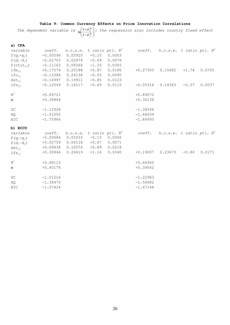
The first parts of the two tables report the CFA regressions. For ijp the regression results

are rather different from those for Sij. There are two differences between the equations. First, the

border dummy ifbij is significant in the ijp regression. Countries sharing a common border have

higher values of ijp. The point estimate on the dummy is 0.18. In other words, neighboring

countries can be expected to have a conditional price correlation that is about 18% higher than for

more distant country pairs. Secondly, the monetary union dummy ifsij is statistically insignificant in

the ijp regression. In other words, if we condition out that part of price changes due to exogenous

shocks to foreign prices, or to shocks to domestic money supply and output, the correlations in price

changes across countries do not depend on whether two counties are part of the same monetary

union. As we will see below, cross-country correlations in output shocks are independent of ifsij,

and the foreign price shocks are common to all CFA countries. So the reason for the difference

between the two equations lies in the monetary shocks. Price movements in countries within a

monetary union are more highly correlated with each other than they are with price movements in

the countries of the other union; but this appears to be largely because countries within a monetary

union are subject to a single central bank with a single monetary policy. There is no evidence for

“deeper” market integration within a union.

We find a similar phenomenon in the Caribbean sample. The non-linear combination of distij

and ifsij that explained a large part of the variation in Sij across countries is not significant in the

ijp regression. In the linear regression equation reported in Table 9, there is no sign of any non-

linearity, and neither distij nor ifsij is statistically significant. The effects of monetary union

membership are apparent only when we are looking at the correlation of unconditional price

movements.

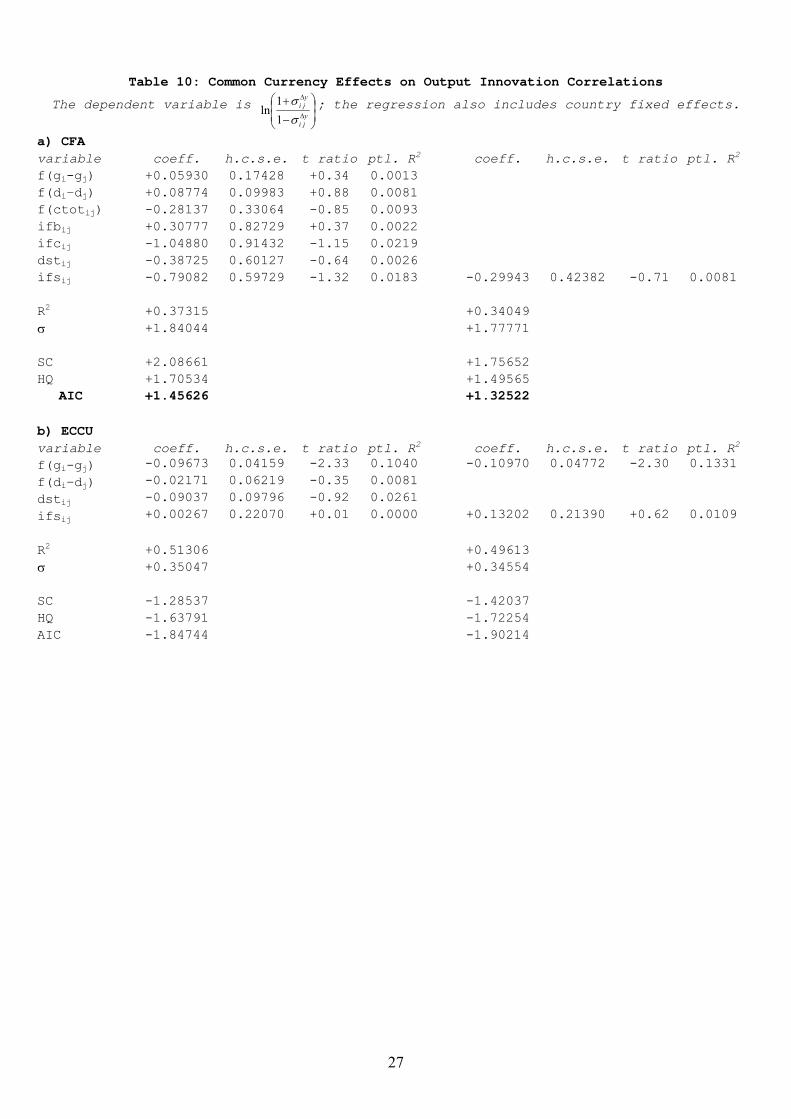
Table 10 shows that there is no evidence that membership of the same monetary union

increases the extent of business cycle correlation, as measured by the correlation of output

innovations in each country, ijy. There is some evidence, at least in the Caribbean, that exogenous

characteristics such as the structure of production do affect this correlation. In the Caribbean sample

17

the coefficient on f(| gi - gj |) is –0.097, which is significantly different from zero. The sample

standard deviation of this variable is 1.154, so the estimated coefficient on this variable implies that

two countries with an atypically high difference in the structure of production (say, two standard

deviations above the mean) can be expected to have an output innovation correlation that is about 22%

lower than average. When one conditions the cross-country correlation of output shocks on these

structural characteristics, the ifsij dummy plays no significant role.

6. Summary and Conclusion

In this paper we have explored the factors that determine the degree of macroeconomic integration

in two areas of the world: the CFA Franc Zone and the Caribbean, including the East Caribbean

Currency Union. All of the countries in our two samples have maintained a pegged exchange rate

over the last 40 years (to the French Franc and US Dollar respectively). Some of them share the

same currency. Our aim has been to see whether sharing a common currency delivers an extra

degree of macroeconomic integration, as compared with sharing a common peg. Four indicators of

integration are considered: trade intensity, unconditional real exchange rate volatility, and the

correlation of innovations in domestic prices and real output.

The evidence on the effect of a single currency is mixed. In the CFA, sharing a common

currency is associated with substantially more bilateral trade, but only among the countries that are

landlocked. This suggests that capacity of a single currency to reduce the barriers to trade is

entwined with the countries’ geographical characteristics, which are important in determining the

size of transportation costs. In both the CFA and the Caribbean, sharing a common currency is

associated with substantially lower bilateral real exchange rate volatility. In the Caribbean the size

of this effect depends on geographical location. For countries further apart, the effect is stronger.

However, the real exchange rate effects of a single currency disappear when one looks at the

cross-country correlation of shocks to prices, that is, domestic price changes conditional on foreign

(i.e., European or American) price changes, and on changes in domestic output and money. So the

greater degree of correlation of prices within a monetary union probably results from a similarity in

the pattern of changes in aggregate demand (and in particular, in monetary changes) rather than

from greater market integration. Furthermore, there is no evidence that the members of a monetary

experience a greater degree of business cycle convergence, when such convergence is measured in

terms of the correlation of innovations in GDP.

Macroeconomic integration can be measured in a variety of different ways. For some – but

not all – measures, sharing a single currency promotes more integration than can be expected in

countries that just share the same currency peg. In order to decide whether the international policy

co-ordination necessary for full monetary union is worth the effort, we need to know which kinds of

18

integration are the most relevant in evaluating social welfare. Even then, the size of the single

currency effect will not be independent of the geographic and economic characteristics of the

countries concerned.

19

References

J. Anderson and van Wincoop, E. (2001) "Gravity with Gravitas: A Solution to the Border Puzzle", NBER Working

Paper 8079

M. Artis and Zhang, W. (1995) "International Business Cycles and the ERM: Is there a European Business Cycle?",

CEPR Discussion Paper 1191

L. Boone (1997) "Symmetry and Asymmetry of Supply and Demand Shocks in the European Union: A Dynamic

Analysis", CEPII Working Paper 97-03

T. Bayoumi and Eichengreen, B. (1996) "Operationalizing the Theory of Optimal Currency Areas", mimeo, CEPR,

London, UK

O. Blanchard and Quah, D. (1989) "Dynamic Effects of Aggregate Demand and Supply Disturbances", American

Economic Review, 79, P655-73

M. Bruno and Easterly, W. (1998) "Inflation Crises and Long Run Growth", Journal of Monetary Economics, 41, 3-

26

N. Christodoulakis, Dimelis, S. and Kollintzas, T. (1995) "Comparisons of Business Cycles in the EC:

Idiosyncracies and Regularities", Economica, 62, 1-27

P. De Grauwe (2000) Economics of Monetary Union: Oxford University Press, Oxford, England.

C. Engel and Rogers, J. (2001) "Deviations from Purchasing Power Parity: Causes and Welfare Costs", Journal of

International Economics, 55, 29-57

A. Fatas (1996) "EMU: Countries or Regions?", paper presented to the European Economic Association Annual

Conference, Istanbul

D. Fielding and Shields, K. (2001) "Modeling Macroeconomic Shocks in the CFA Franc Zone", Journal of

Development Economics, 66, 199-223

S. Fischer (1993) "The Role of Macroeconomic Factors in Growth", Journal of Monetary Economics, 32, 485-512

L. Goreux, A. Ghosh , Gulde, A-M., Ostry, J. and Wolf, H. (1995) "Currency Boards: The Ultimate Fix?", IMF

Working Paper WP/95/121

J. Green and Villanueva, D. (1990) "Private Investment in Developing Countries", IMF Staff Papers, 38, 33-58

J. Lothian and Taylor, M. (1996) "Real Exchange Rate Behavior: The Recent Float from the Perspective of the Past

Two Centuries", Journal of Political Economy, 104, 448-509

M. Obstfeld and Rogoff, K. (1996) Foundations of International Macroeconomics: MIT Press, Cambridge, MA

D. Papell (1997) "Searching for Stationarity: Purchasing Power Parity Under the Current Float", Journal of

International Economics, 43, 313-32

T. Persson (2001) "Currency Unions and Trade : How Large is the Effect?", Economic Policy, 33

A. Rose (2001) "Currency Unions and Trade : the Effect is Large", Economic Policy, 33

A. Rose and Engel, C. (2000) "Currency Unions and International Integration", NBER Working Paper 7282

A. Rose and van Wincoop, E. (2001) "The Real Case for Currency Union", American Economic Review (papers

and proceedings), 91, 386-90

M. Vizy (1989) La Zone Franc: CHEAM, Paris, France

20

Table 1: Trade Statistics for CFA Members

Figures are for the most recent year available in IFS DOTS

CountryExports to LDCs

(% Total Exports)

Imports from LDCs

(% Total Imports)

Benin 06 29

Burkina Faso 58 48

Cameroon 28 33

Centrafrique 18 31

Chad 15 44

Congo Republic 72 31

Côte d’Ivoire 45 54

Gabon 22 12

Mali 45 64

Niger 47 52

Senegal 49 44

Togo 80 69

Table 2: Monetary Groupings in the CFA and the Caribbean

Countries in italics are excluded from the econometric analysis because of inadequate data (i.e., the relevant economic time-series in World Bank World Development Indicators are incomplete).

1. CFA Countries (2 separate currencies)

UEMOA: Benin, Burkina Faso, Cote d’Ivoire, Guinea-Bissau, Mali, Niger, Senegal, Togo

UDEAC: Cameroon, C.A.R., Chad, Congo Republic, Equatorial Guinea, Gabon

2. Caribbean & Central American Countries (4 separate currencies)

ECCU: Antigua & Barbuda, Aruba, Dominica, Grenada, Montserrat, St. Kitts & Nevis, St. Lucia, St. Vincent & the Grenadines

Separate: Barbados, Belize US$ pegs

Dollarized: The Bahamas, Panama

21

Table 3: Summary Statistics

ben bfa civ sen tgo mli ner cam cgo gab car tcd

1987 agriculture value added (% GDP) 33.3 31.5 29.2 21.7 33.5 45.2 36.3 24.8 11.9 11 46.9 33.1 1997 agriculture value added (% GDP) 38.4 31.8 27.3 18.5 42.2 44.0 38.0 42.1 9.5 7.5 54.1 37.4

1987 total external debt (% GDP) 76.4 38.4 134.6 87.6 98.9 94.2 75.1 33.2 145.2 79.8 47.8 27.9 1997 total external debt (% GDP) 75.9 54.5 152.3 81.0 89.2 119.9 88.7 101.9 227 67.5 92.3 54.9

1987 exports (% GDP) 29.3 10.6 33.4 24.1 41.4 16.6 21.5 15.7 41.7 42.7 16.2 15.4 1997 exports (% GDP) 24.9 11.2 46.6 32.8 34.7 25.5 16.2 26.8 77.0 64.0 19.5 18.7

1985 gross investment (% GDP) 12.9 20.9 12.3 12.5 17.6 20.7 12.0 24.7 19.7 26.4 12.5 9.1 1995 gross investment (% GDP) 18.5 27.0 16.0 18.7 14.9 20.6 10.8 16.2 26.0 26.3 9.0 16.3

sample s.d. y (%) 4.5 4.0 6.3 3.8 7.4 5.3 9.0 5.7 6.9 9.0 4.2 11.4 sample s.d. p (%) 8.0 8.1 6.8 7.9 8.0 10.0 9.1 7.2 7.8 9.0 6.5 8.0 sample s.d. m (%) 30.0 9.9 10.5 16.0 34.3 11.1 13.6 13.1 13.7 16.8 13.7 16.8

atg dma grd ktn lca vct bhs brb blz pan

1985 agriculture value added (% GDP) 5.0 28.0 17.1 9.1 15.2 19.6 2.2 6.2 20.4 8.81995 agriculture value added (% GDP) 3.8 20.4 10.1 5.3 10.5 14.1 —— —— 20.7 8.4

1985 exports (% GDP) 88.6 36.5 43.0 55.4 55.9 73.0 64.8 67.8 48.5 68.61995 exports (% GDP) 85.9 46.8 45.4 49.6 67.6 53.1 —— —— 49.8 100.7

1985 gross investment (% GDP) —— 28.5 26.6 30.3 21.0 28.0 19.2 15.4 21.6 15.21995 gross investment (% GDP) 46.7 32.6 32.1 46.0 19.0 33.2 —— —— 20.0 30.3

1985 total external debt (% GDP) —— 55.1 40.7 16.4 10.6 22.0 —— 38.1 56.6 88.11995 total external debt (% GDP) —— 44.6 40.8 24.2 22.6 78.4 —— 34.3 44.0 79.4

sample s.d. y (%) 3.56 6.07 5.57 3.61 7.2 5.22 6.84 3.76 1.0 4.46sample s.d. p (%) 3.42 4.57 4.13 4.46 4.81 3.33 2.17 4.32 0.97 4.09

Source: World Bank World Development Indicators 1999. y: GDP growth rate; p: inflation; m: money supply growth rate

22

Table 4: Common Currency Effects on Trade Intensity in the CFA The dependent variable is ln(1+T); the regression also includes country fixed effects.

variable coeff. h.c.s.e. t ratio ptl. R2 coeff. h.c.s.e. t ratio ptl. R2

yi·yj -0.42693 0.28202 -1.51 0.0423 -0.45123 0.27857 -1.62 0.0900 ypi·ypj +0.60948 0.44724 +1.36 0.0261 +0.74544 0.35529 +2.10 0.0900 ai·aj -0.17426 0.15384 -1.13 0.0259 ifbij +1.52930 0.45887 +3.33 0.2178 +1.45650 0.49910 +2.92 0.3100 ifcij +0.09240 0.58497 +0.16 0.0005 dstij -0.67841 0.78537 -0.86 0.0179 -0.72519 0.41628 -1.74 0.1000 ifsij -0.61079 0.83264 -0.73 0.0104 ifs·dstij -0.23643 0.58419 -0.40 0.0035 ifs ifcij +1.08890 0.46108 +2.36 0.1050 +0.92816 0.33192 +2.80 0.2000 R2 +0.90193 +0.89768

NORM +1.99250 +2.50240 SC +0.56959 +0.35810 HQ +0.14819 +0.01697 AIC -0.12712 -0.20590

Table 5: RESET Tests for Functional Form Specification (All Equations)

CFA Equation Unrestricted Model Restricted Model ln(1+T) F(3,53) = 0.88303 [0.4559] F(3,58) = 0.37202 [0.7735] S F(3,56) = 0.05133 [0.9845] no conditioning variables

p F(3,56) = 0.39742 [0.7554] F(3,61) = 0.02746 [0.9938] y F(3,56) = 0.40897 [0.7472] no conditioning variables

ECCU Equation Unrestricted Model Restricted Model S F(3,37) = 0.32188 [0.8095] F(3,39) = 0.13441 [0.9390]

p F(3,38) = 0.72641 [0.5426] no conditioning variables y F(3,38) = 0.86249 [0.4689] F(3,40) = 0.65188 [0.5865]

23

Table 6: Common Currency Effects on Unconditional Real Exchange Rate Volatility The dependent variable is S; the regression also includes country fixed effects.

a) CFA variable coeff. h.c.s.e. t ratio ptl. R2 coeff. h.c.s.e. t ratio ptl. R2

f(gi-gj) -0.03056 0.04360 -0.70 0.0087 f(di–dj) -0.00368 0.01830 -0.20 0.0004 f(ctotij) -0.07051 0.07909 -0.89 0.0150 ifbij -0.09241 0.17186 -0.54 0.0052 ifcij +0.08370 0.18530 +0.45 0.0037 dstij -0.22236 0.18746 -1.19 0.0216 ifsij -0.29545 0.15422 -1.92 0.0629 -0.19710 0.09377 -2.100 0.0832

R2 +0.57533 +0.54916

+0.36208 +0.35132 SC -1.16519 -1.48627 HQ -1.54646 -1.74714 AIC -1.79554 -1.48627

b) ECCU variable coeff. h.c.s.e. t ratio ptl. R2 coeff. h.c.s.e. t ratio ptl. R2

f(gi-gj) -0.03379 0.03593 -0.94 0.0265 f(di–dj) -0.00654 0.02344 -0.28 0.0015 dstij +0.74303 0.09503 +7.82 0.7094 +0.73502 0.09911 +7.42 0.7008ifsij -1.50370 0.49233 -3.05 0.2780 -1.57190 0.43479 -3.62 0.2965ifs·dstij -0.53765 0.19065 -2.82 0.3126 -0.55655 0.17279 -3.22 0.3252

R2 +0.87922 +0.87553

+0.25446 +0.25012 SC -1.87379 -2.01286 HQ -2.25150 -2.34022 AIC -2.47601 -2.53479

24

Table 7: Structural Innovation Correlations (For y above the diagonal and p below. *** significantly different from zero at 1%; ** at 5%; * at 10%)

ben bfa sen tgo ner cam gab car tcd civ mli cgo Ben 0.47*** 0.13 0.56*** 0.38** 0.52*** 0.48*** 0.31* 0.28 -0.58*** -0.48*** -0.50*** Bfa 0.74*** 0.68*** 0.78*** 0.76*** 0.69*** 0.84*** 0.54*** 0.67*** -0.73*** -0.77*** -0.83*** Sen 0.72*** 0.89*** 0.58*** 0.79*** 0.56*** 0.63*** 0.40*** 0.55*** -0.56*** -0.64*** -0.68*** Tgo 0.82*** 0.84*** 0.91*** 0.85*** 0.81*** 0.90*** 0.67*** 0.77*** -0.87*** -0.93*** -0.93*** Ner 0.41** 0.47*** 0.41** 0.50*** 0.76*** 0.82*** 0.58*** 0.65*** -0.80*** -0.83*** -0.90*** Cam 0.75*** 0.81*** 0.94*** 0.89*** 0.27 0.87*** 0.62*** 0.69*** -0.74*** -0.76*** -0.83*** Gab 0.75*** 0.87*** 0.95*** 0.90*** 0.39** 0.96*** 0.69*** 0.75*** -0.82*** -0.88*** -0.93*** Car 0.77*** 0.84*** 0.97*** 0.93*** 0.39** 0.95*** 0.97*** 0.61*** -0.42*** -0.57*** -0.66*** Tcd 0.67*** 0.56*** 0.56*** 0.59*** 0.25 0.63*** 0.61*** 0.60*** -0.61*** -0.79*** -0.80*** Civ 0.82*** 0.89*** 0.90*** 0.90*** 0.46*** 0.91*** 0.92*** 0.91*** 0.64*** 0.86*** 0.87*** Mli 0.74*** 0.81*** 0.92*** 0.91*** 0.47*** 0.89*** 0.94*** 0.94*** 0.66*** 0.86*** 0.94*** Cgo 0.74*** 0.86*** 0.94*** 0.90*** 0.44*** 0.91*** 0.92*** 0.95*** 0.69*** 0.89*** 0.91***

atg dma grd ktn lca vct bhs brb blz pan

Atg 0.292 0.375** 0.631*** 0.107 0.188 0.086 0.150 0.062 -0.011

Dma 0.681*** 0.006 0.234 0.200 0.309* 0.133 -0.034 0.320* -0.249

Grd 0.248 0.586*** 0.229 -0.156 0.328* 0.316* 0.364* 0.055 0.108

Ktn 0.454** 0.321* 0.256 0.332* -0.036 0.122 0.162 0.248 -0.148

Lca 0.026 0.072 -0.204 0.087 0.220 0.139 0.407** 0.289 -0.291

Vct 0.062 -0.145 0.023 0.235 -0.209 0.132 0.008 0.326** -0.310*

Bhs 0.202 -0.061 -0.233 0.124 -0.107 0.132 0.283* 0.040 0.117

Brb 0.672*** 0.520*** 0.503*** 0.313** -0.265 -0.191 0.142 0.006 -0.025

Blz 0.386** 0.483*** 0.487*** 0.219 -0.190 -0.114 -0.177 0.579*** -0.193

Pan 0.084 0.124 0.239 0.147 -0.176 -0.169 -0.056 0.367* 0.244

25

Table 8: Identification of “Core Groups”

The table shows the mean value of cross-country correlations in either price innovations (1) or

output innovations (2) for different “core groups” of countries. Corresponding standard deviations

(S.D.) are also shown, along with the percentage of correlations significantly greater than zero (% Sig.).

Core Group Mean Corr. S.D. Corr. % Sig. CFAPrices Group #1 ben, bfa, civ, sen, tgo, mli, 0.759 0.194 96

ner, cam, cgo, gab, car, tcd

Prices Group #2 civ, sen, tgo, mli, cam, cgo, 0.921 0.026 100 gab, car

Output Group #1 ben, bfa, sen, tgo, ner, cam, 0.629 0.175 100 gab, car, tcd

Output Group #2 civ, mli, cgo 0.890 0.036 100

CaribbeanPrices Group #1 atg, dma, grd, ktn, brb, blz, 0.377 0.174 57

pan

Prices Group #2 atg, dma, grd, brb, blz 0.515 0.123 90

Output Group #1 atg, dma, grd, ktn, lca, vct, 0.191 0.155 31 bhs, brb, blz

26

Table 9: Common Currency Effects on Price Innovation Correlations

The dependent variable is pji

pji

11

ln ; the regression also includes country fixed effect

a) CFA variable coeff. h.c.s.e. t ratio ptl. R2 coeff. h.c.s.e. t ratio ptl. R2

f(gi-gj) -0.00596 0.05910 -0.10 0.0003 f(di–dj) -0.01703 0.02474 -0.69 0.0076 f(ctotij) -0.11163 0.08364 -1.33 0.0355 ifbij +0.17574 0.20188 +0.87 0.0180 +0.27305 0.15682 +1.74 0.0705ifcij -0.13388 0.24138 -0.55 0.0090 dstij -0.16997 0.19911 -0.85 0.0123 ifsij -0.12549 0.18117 -0.69 0.0115 -0.05316 0.14343 -0.37 0.0037

R2 +0.89721 +0.89072

+0.36864 +0.36136 SC -1.12928 -1.38546 HQ -1.51055 -1.66639 AIC -1.75964 -1.84993

b) ECCU variable coeff. h.c.s.e. t ratio ptl. R2 coeff. h.c.s.e. t ratio ptl. R2

f(gi-gj) -0.00684 0.05433 -0.13 0.0006 f(di–dj) +0.02759 0.04118 +0.67 0.0071 dstij +0.09438 0.10574 +0.89 0.0218 ifsij +0.30846 0.26619 +1.16 0.0340 +0.19007 0.23673 +0.80 0.0171

R2 +0.68113 +0.66940

+0.40176 +0.39062 SC -1.01216 -1.22983 HQ -1.36470 -1.50682 AIC -1.57424 -1.67146

27

Table 10: Common Currency Effects on Output Innovation Correlations

The dependent variable is yji

yji

11

ln ; the regression also includes country fixed effects.

a) CFA variable coeff. h.c.s.e. t ratio ptl. R2 coeff. h.c.s.e. t ratio ptl. R2

f(gi-gj) +0.05930 0.17428 +0.34 0.0013 f(di–dj) +0.08774 0.09983 +0.88 0.0081 f(ctotij) -0.28137 0.33064 -0.85 0.0093 ifbij +0.30777 0.82729 +0.37 0.0022 ifcij -1.04880 0.91432 -1.15 0.0219 dstij -0.38725 0.60127 -0.64 0.0026 ifsij -0.79082 0.59729 -1.32 0.0183 -0.29943 0.42382 -0.71 0.0081

R2 +0.37315 +0.34049

+1.84044 +1.77771 SC +2.08661 +1.75652 HQ +1.70534 +1.49565

AIC +1.45626 +1.32522

b) ECCU variable coeff. h.c.s.e. t ratio ptl. R2 coeff. h.c.s.e. t ratio ptl. R2

f(gi-gj) -0.09673 0.04159 -2.33 0.1040 -0.10970 0.04772 -2.30 0.1331f(di–dj) -0.02171 0.06219 -0.35 0.0081 dstij -0.09037 0.09796 -0.92 0.0261 ifsij +0.00267 0.22070 +0.01 0.0000 +0.13202 0.21390 +0.62 0.0109

R2 +0.51306 +0.49613

+0.35047 +0.34554 SC -1.28537 -1.42037 HQ -1.63791 -1.72254 AIC -1.84744 -1.90214

28

Figure 1: The CFA Franc Zone

The dark shaded area is the UEMOA; the light shaded area is the UDEAC.

1 = Benin; 2 = Burkina Faso; 3 = Côte d’Ivoire; 4 = Guinea-Bissau; 5 = Mali; 6 = Niger; 7 = Senegal; 8 = Togo 9 = Cameroon; 10 = C.A.R.; 11 = Chad; 12 = Congo Republic; 13 = Gabon; 14 = Equatorial Guinea

Ga = Gambia; Gh = Ghana; Gu = Guinea-Conakry; L = Liberia; M = Mauritania; N = Nigeria; S = Sierra Leone