do housing values respond to underground storage tank ... · matthew ranson2, and ... the purpose...

Working Paper Series

U.S. Environmental Protection Agency National Center for Environmental Economics 1200 Pennsylvania Avenue, NW (MC 1809) Washington, DC 20460 http://www.epa.gov/economics

Do Housing Values Respond to Underground

Storage Tank Releases?

Evidence from High-Profile Cases across the United States

Dennis Guignet, Robin R. Jenkins,

Matthew Ranson and Patrick J. Walsh

Working Paper # 16-01

March, 2016

Do Housing Values Respond to

Underground Storage Tank Releases?

Evidence from High-Profile Cases across the United States

Dennis Guignet*1, Robin R. Jenkins1,

Matthew Ranson2, and Patrick J. Walsh1

NCEE Working Paper Series

Working Paper # 16-01

March, 2016

*Corresponding Author

National Center for Environmental Economics

US Environmental Protection Agency

Mail Code 1809 T

1200 Pennsylvania Avenue, N.W.

Washington, DC 20460, USA

Phone: +1-202-566-1573

[email protected]

1 National Center for Environmental Economics, U.S. EPA

2 Abt Associates Inc.

DISCLAIMER

The views expressed in this paper are those of the author(s) and do not necessarily represent those of the

U.S. Environmental Protection Agency. In addition, although the research described in this paper may

have been funded entirely or in part by the U.S. Environmental Protection Agency, it has not been

subjected to the Agency's required peer and policy review. No official Agency endorsement should be

inferred.

1

ABSTRACT

Underground storage tanks (USTs) containing petroleum and hazardous substances are ubiquitous.

Accidental releases of these substances can present risks to local residents and the environment.

The purpose of this paper is to develop monetized estimates of the benefits of preventing and

cleaning up UST releases, as reflected in house values. We focus on 17 of the most high-profile

UST releases in the United States with release discovery and other milestone events occurring at

different points between 1985 and 2013. These data are the broadest analyzed for property value

impacts of UST releases, as previous hedonic studies of USTs focused only on a single county,

city, or subset of counties within a state. We employ a two-step methodology in which (i) site

specific hedonic regressions are estimated using a difference-in-differences approach, and then (ii)

an internal meta-analysis of the resulting estimates is conducted. The spatial and temporal

variation among the 17 sites improves our identification of the treatment effects by reducing local

idiosyncratic biases; thus providing greater confidence to a causal interpretation of the estimated

average price effects. The results suggest significant heterogeneity in the price effects across sites,

but on average reveal a 3% to 6% depreciation upon the discovery of a high profile release, and a

similar appreciation after cleanup. These average effects diminish with distance, extending out to

2 or 3km from the site.

JEL Classification: Q24; Q51; Q53

Keywords: groundwater; hedonic; meta-analysis; property value; underground storage tank; UST;

vapor intrusion

ACKNOWLEDGEMENTS

This research was supported by funding from the U.S. Environmental Protection Agency’s (EPA) Office

of Underground Storage Tanks (OUST). We are grateful to Abt Associates and Angel Kosfiszer for data

support, and to Sarah Marrinan for excellent research assistance. We thank staff in EPA’s OUST, Office

of Research and Development, and Regional Offices as well as state and local environmental agencies for

information on UST releases and the federal UST Program. We thank Heather Klemick, Alex Marten, and

participants at the Northeastern Agricultural and Resource Economics Association’s 2015 Annual

Conference for helpful comments.

1

I. INTRODUCTION

Underground storage tanks (USTs) containing petroleum and hazardous substances are

ubiquitous, usually associated with gas stations and occasionally with industrial facilities. In the

United States, there are over half a million active USTs, and almost two million that are no longer

in use (US Environmental Protection Agency, 2011). More than half a million of these active and

inactive USTs have been associated with leaks that release chemicals into the environment.1 Due

to state and federal regulations requiring release prevention and detection activities, most UST

releases are small in scope and far from being headline news. However, chemicals released from

USTs can cause fires, explosions, neurological damage, blood disorders, cancer, and other adverse

health outcomes (Jenkins et al., 2014). UST release events may involve contaminated

groundwater, vapor emissions and intrusions, and/or contaminated surface water. Thus, UST

releases sometimes garner significant press coverage and elicit public concern regarding potential

risks to human health and the environment.

The purpose of this paper is to develop monetized estimates of the benefits of preventing

and cleaning up UST releases, as capitalized in local residential property values. A few previous

studies have used hedonic methods to measure the impacts of UST releases on nearby housing

values (Guignet, 2013; Isakson & Ecker, 2013; Simons et al., 1997; Zabel & Guignet, 2012).

However, because potential homebuyers typically have little or no information about nearby

releases, identifying the property value impacts of UST leaks is difficult. To address this empirical

challenge, our study focuses on 17 sites in the United States where high-profile UST releases were

widely publicized and involved significant community concern. These sites are drawn from

communities ranging from California to the East Coast, and represent some of the most highly

1 According to the federal EPA Office of Underground Storage Tanks (OUST), since 1984, 520,000 releases have

been reported and 74,000 remain to be cleaned up (US Environmental Protection Agency, 2014).

2

publicized—and at most sites, severe—UST leak events that have occurred in the United States

over the last thirty years. Thus, these incidents provide a compelling empirical context in which to

measure the monetary tradeoffs that homeowners are willing to make to avoid or accept risks from

UST leaks.

Our analysis uses a two-step methodology that involves site-specific hedonic regressions

followed by an internal meta-analysis of the resulting estimates. First, at each site, we use hedonic

regressions to estimate how housing prices changed in the wake of publicized milestone events.

We identify four types of milestones: initial discovery of the release, completion of cleanup, “other

positive” events (such as announcements about future remediation plans), and “other negative”

events (such as discovery of additional contamination).

To control for pre-existing site-specific trends in housing prices, our regressions use a

difference-in-differences (DID) approach that compares the change in prices in neighborhoods

near the leak site against the change in prices in neighborhoods located further from the site. To

allow for the possibility that homeowners’ perceptions of risk vary by distance, we define five

distinct “treatment” neighborhoods for each site, using houses located 0-1 km, 1-2 km, 2-3 km, 3-

4 km, and 4-5 km from the leak site. Houses located 5-10 km from the site serve as the control

group.

After estimating the change in house prices after each milestone event for each treatment

group at each site, we then use an internal meta-analysis to summarize property value impacts

across the 17 sites. This meta-analysis combines the coefficients and statistical uncertainty from

each hedonic regression to estimate an aggregate distribution of the percent changes in housing

values from leaking USTs.

3

Our results suggest that the impact of an UST release on property values varies

considerably across sites and milestone events. However, on average, during the five-year period

following the discovery of a release there is a 3% to 6% decrease in housing values. The effects

diminish with distance from the site, but houses as far as 2 or3 km away still experience a decrease

in value. Additionally, looking at sales within 5 years after a cleanup, on average property prices

rebound by 4% to 9%, an effect that also diminishes with distance. Nonetheless, we do observe

considerable heterogeneity in how property values respond to both discoveries and clean-ups, with

some events appearing to cause very large property value changes, and others appearing to cause

negligible changes, or a counterintuitive effect.

Our paper advances existing research in three ways. First, our study is the broadest study

ever conducted of the property value effects of UST releases. To support our analysis, we have

assembled comprehensive microdata covering 17 high-profile release sites from communities

across the United States. In contrast, past hedonic studies of UST releases have focused only on a

single county, city, or subset of counties within a state (Guignet, 2013; Isakson & Ecker, 2013;

Simons et al., 1997; Zabel & Guignet, 2012). The previous work that is most similar to ours is a

study of Maryland by Zabel and Guignet (2012), which found that UST releases only impacted

house prices when leaks were publicized and the community was informed about potential risks.

Second, by focusing exclusively on high-profile incidents, our study circumvents broader

concerns from the land contamination literature about whether property market participants are

aware of the disamenity of interest, UST releases in this case (Guignet, 2013). Of course, this

focus on high-profile UST sites also results in estimates that represent the upper range of property

value impacts, relative to the population of UST releases. Thus, our estimates are not readily

4

transferable to a typical UST release. Nonetheless, the results do inform policymakers about the

upper reaches of benefits to nearby residents of actions to prevent and clean up UST releases.

Our third contribution is a useful combination of quasi-experimental methods with meta-

analytic techniques within a single study to improve identification of the treatment effect. The

DID model used to estimate site-specific treatment effects relies on the assumption that in the

absence of a UST-related event, the outcome of interest (in our case housing prices) would have

followed similar trends in both the control and treated groups (Gamper-Rabindran and Timmins,

2013). This assumption could be violated if unobserved influences on house prices are correlated

with proximity to the site and the timing of events. Our diagnostic analysis of pre-event price

trends suggests that for some sites in our sample, the estimated treatment effects could be

confounded by local trends in the housing market.

However, our use of multiple sites in a meta-analytic framework allows us to generate

robust estimates of the average property value impacts, reducing the influence of local unobserved

trends at individual sites. Our 17 high-profile releases occurred in different housing markets across

the period from 1985 to 2013. This spatial and temporal variation in the treatment of interest (i.e.,

the release, cleanup, or other milestone events) allows us to use meta-analysis to essentially

“average” out any idiosyncratic biases; thereby lending greater confidence to a causal

interpretation of the estimated average price effects. We present meta-regression estimates from

random effect-size models, which account for unobserved or unmeasured factors that might

influence the estimates from individual sites (Nelson, 2015).

The remainder of this paper is organized as follows. Section II presents a brief review of

the hedonic property value literature on contaminated sites. Section III describes how we selected

our high-profile sites and explains our hedonic property value model and internal meta-analysis.

5

Section IV describes the data used to estimate the empirical models. Finally, Sections V and VI

present our results and concluding remarks.

II. LITERATURE REVIEW

An extensive literature exists on how contaminated sites have affected surrounding

property values. Papers have studied the impact of proximity to (or risk of) a nearby contaminated

site; or property value changes over time, targeting discovery of contamination, completion of

cleanup, or other milestones related to a single site.2 Many hedonic studies have focused on

property values around a small set of sites (e.g., Kohlhase (1991), Kiel (1995), Messer et al.

(2006)), but recently the importance of analyzing national samples of contaminated sites has been

emphasized, with studies examining sites receiving federal Environmental Protection Agency

(EPA) brownfields grants (Haninger et al., 2014 ) and sites on the EPA National Priorities List

(NPL) (Gamper-Rabindran & Timmins, 2013; Greenstone & Gallagher, 2008; Kiel, Katherine A.

& Micheal Williams, 2007).

A. Property Value Impacts when Households are Informed

A sizable portion of the literature on the property value impacts of contamination has

focused on Superfund NPL sites. These sites are subject to a formal sequence of actions, including

proposal to list, final listing, and cleanup completion, among others. The public is likely to be

relatively well informed about nearby NPL sites as public notification is required at many steps

along the timeline of actions. For example, EPA publishes in the Federal Register any proposal to

list a site on the NPL, and notifies the local press (US Environmental Protection Agency, 2015).

2 See Banzhaf and McCormick (2007), Boyle and Kiel (2001), Sigman and Stafford (2011) and US Environmental

Protection Agency (2009) for reviews.

6

Several early papers (e.g., Michaels and Smith (1990), Kohlhase (1991), Kiel (1995)) examined

multiple Superfund sites and generally found that subsequent to discovery or listing, there was a

positive correlation between distance from a site and property values, suggesting households were

willing to pay a premium to be located further from contamination. However, there is mixed

evidence of the price effects of cleanup (Dale et al., 1999; Kiel, Katherine A. & Micheal Williams,

2007; Kohlhase, 1991; McCluskey & Rausser, 2003a), particularly when remedial efforts are

prolonged over long periods of time (Messer et al., 2006).3

With the goal of investigating beyond only high-profile cases, Kiel and Williams (2007)

examined all NPL sites in 13 US counties to learn whether property value impacts were similar

across sites. They examined two assertions that previously had been made in the literature: (i)

proximity to an NPL site lowers property values, and (ii) cleaning up an NPL site restores property

values. Using residential property transaction data from 1970 through 1996, they studied six

timeframes4 but focused on listing. The paper concluded that NPL listing at some sites (18 of 57)

had the expected negative impact on house prices, but at others had no impact (32 of 57) or even

a positive effect (the remaining 7).

B. UST Releases and Residential Property Values

Compared to NPL sites, the typical UST release can often be considered a relatively small

disamenity. Nonetheless, UST releases can still pose risks to human health and the environment.

There are three exposure paths through which UST releases can lead to health and environmental

3 A few hedonic property value studies have gone beyond the conventional identification strategy of examining how

the distance gradient changes after key milestones. For example, Gayer and Viscusi (2002) examined whether news

stories raised alarm bells or quelled concerns about contaminated land. 4 The timeframes were pre-discovery; discovery through NPL proposal; proposal through NPL listing; listing through

beginning of cleanup; cleanup through removal from NPL; and post-removal.

7

risks. First, gasoline and hazardous additives can infiltrate local groundwater aquifers, which in

some cases are key water sources for private wells and public water systems. Such contamination

poses health risks from ingestion, skin contact, and inhalation of fumes, all of which may cause

neurological damage, blood disorders, cancer, and other adverse health outcomes (Jenkins et al.,

2014). A second common contamination pathway occurs when vapors emitted from released

gasoline migrate through soil, septic, or drainage pipes and into structures. This type of

contamination poses acute health risks and a risk of fire or explosion. Finally, contaminated runoff

can migrate into surface water directly, creating environmental problems and threatening local

ecosystems.

There are a few studies that examined the impact of USTs releases on surrounding

residential property values. Focusing on Cuyahoga County, Ohio, Simons et al. (1997) estimated

a hedonic model using a cross-section of house sales in 1992 and found a 17% depreciation among

houses within 300 feet of a registered leaking UST. Focusing on house sales from 1994-1996 in

that same county, Simons et al. (1999) found that “contamination” from nearby gas stations

reduced house values by 14% to 16%.5 In a working paper, Isakson and Ecker (2010) examined

50 USTs in Cedar Falls, Iowa, and found that the prices of houses adjacent to UST releases

classified as “high risk” by regulators were about 11% lower. Due to the small samples and cross-

sectional data, the results of these studies should be interpreted with caution.

Zabel and Guignet (2012) exploited both spatial and temporal variation in house prices in

order to identify the causal impact of UST releases. Focusing on three counties in Maryland they

5 Simons et al. (1999) defined contamination based on a 3-point scale, where 1= well test confirmed contamination at

the house, 2= house was adjacent and down-gradient from a LUST, and 3= house was adjacent to a house scored as

‘1’ or ‘2’, down-gradient, and within 50-100 ft of the contamination plume. Only 11 contaminated houses were sold

which is too few for a typical hedonic study. Instead they compared the actual transaction prices to house-specific

predicted prices from a hedonic regression that did not explicitly account for leaking UST sites.

8

concluded that the typical (i.e., not high-profile) release had no adverse effect on house values.

However, focusing on a subset of the most severe and publicized cases, Zabel and Guignet (2012)

found that when a release was discovered, house values within one kilometer decreased by 5%. In

a follow-up study of the same house transaction data, Guignet (2013) again found no adverse price

impacts associated with the typical release, but did find an 11% depreciation among houses where

the private well was tested for contamination, and thus where the household was well-informed of

the disamenity. Together these studies suggest that residential property values are only impacted

by UST releases when the public is informed, and/or when actual or perceived risks may be higher

than typical.

Existing hedonic property value studies of UST releases are limited to one or a few

localities. There have been several recent nationwide property value analyses of Superfund and

brownfield sites (Gamper-Rabindran & Timmins, 2013; Haninger et al., 2014 ). Given past

findings that the typical UST release does not adversely impact surrounding house values, the

understanding gained by gathering and analyzing a nationwide sample of UST releases would

likely be limited.6 The question remains however as to how consistently highly publicized or

“high-profile” UST releases affect property values. Learning more about these worst case

scenarios helps inform policies to prevent, minimize, and clean up UST contamination.

6 Furthermore, compiling the necessary nationwide dataset of UST releases would be extremely difficult. Data of UST

releases may or may not be maintained by individual states, and not necessarily in a consistent manner. Nationwide

studies of NPL sites (Gamper-Rabindran & Timmins, 2013) and brownfields (Haninger et al., 2014 ), on the other

hand, utilized available nationwide datasets.

9

III. METHODS

A. Selecting High-Profile Release Sites

To identify candidate high-profile release sites we cast a broad net, consulting with EPA’s

Office of Underground Storage Tanks (OUST), all ten EPA Regional Offices, state and local

environmental agencies, and the Association of State and Territorial Solid Waste Management

Officials (ASTSWMO). We also identified several sites through internet searches and by

reviewing ASTSWMO (2012) and relevant academic literature (see Appendix A for details). Our

objective was comprehensive spatial coverage across the contiguous United States.

We initially identified 41 potential high-profile UST sites, located in 23 different states.

Unfortunately, we were not able to study all of these sites. Our focus was on residential properties,

so we eliminated sites in industrial or rural areas where residential development was too sparse for

robust statistical analysis. We eliminated two other sites because the high-profile events were too

recent or too far in the past (with insufficient property transaction data either pre- or post-event).

Finally, after some preliminary research, we eliminated thirteen additional sites due to data and

information constraints; for example, some states (such as Montana) have disclosure laws

preventing the public release of property sales data.

In the end, we obtained sufficient data to examine 17 high-profile UST release sites. Of

these, the majority (nine) represent areas where retail gas stations released gasoline that

contaminated groundwater used in private drinking water wells. At six of the sites vapors migrated

to occupied structures. This was sometimes the sole concern, while other times it added to

groundwater or other risks. For one site, contamination impacted surface water. Three of our sites

had public wells contaminated by UST releases. Finally, methyl tertiary butyl ether (MTBE) (a

10

potentially harmful gasoline additive) was a concern at nine of the 17 sites.7 Appendix A specifies

the original source that identified each high-profile release, offers statistics for the affected

communities, and briefly describes the events surrounding each release site.

Figure 1 presents a map that shows the distribution of these sites across the contiguous

United States. Most sites are located on the East Coast, where the high profile criteria were more

frequently met and data on housing sales were more often available.

B. Hedonic Property Value Model

In the first stage of our analysis, we estimate separate hedonic regressions for each high-

profile site, denoted by s = 1,…, 17. To facilitate a cleaner quasi-experimental comparison and to

ensure comparability of the estimates in the later internal meta-analysis, we adopt restrictions to

improve uniformity across site-level datasets. We use transactions for single-family homes and

townhomes within 10 km of each site. We exclude transactions more than 5 years before or after

each milestone event, since the hedonic equilibrium might shift over time (Kuminoff et al., 2010).

If a site experienced multiple high-profile events that occurred close together in time, then our

hedonic regressions include a separate set of coefficients and variables for each event. However,

if the events were more than five years apart, we split the transaction data into separate datasets,

and estimate individual hedonic regressions for each event.

Since previous literature indicates that the impacts of contamination vary with distance

from the site, we sort houses into discrete one kilometer (km) distance buffers, using functional

7 MTBE is a contaminant and suspected carcinogen that was previously used as a gasoline oxygenate to improve air

emissions. Some states have set limits for MTBE in drinking water and EPA issued a drinking water advisory for it in

1997. MTBE has generally not been used as a gasoline additive since the early 2000s (Jenkins et al., 2014), and so it

is often associated with older, sometimes previously unknown, releases.

11

forms similar to analyses in past literature (Gamper-Rabindran & Timmins, 2013; Zabel &

Guignet, 2012). We allow the potential price impacts associated with proximity to an UST site to

extend out to 5 km.8 The functional form of the hedonic models appears in equation (1).

5

1

ln { }d d d d

ijts ijt s is se tse is t j ijts

d

p x D event D v

M α (1)

The dependent variable, ln pijts, represents the natural logarithm of the price of house i in

neighborhood j at time t near high-profile site s.

The control vector xijt contains all structural, parcel, neighborhood, and other control

variables, including the number of gas stations within 200 and 500 meters of the house. The vector

Mt contains year and quarter fixed effects, vj is a neighborhood fixed effect (at the census tract

level in the presented results), and εijts is a normally distributed, zero-mean error term.

The distance buffers are represented by the dummy variables d

isD , for d = 1,.., 5 km. The

buffers enter the hedonic equation with individual coefficients d

s that account for any differences

in characteristics of houses located at the various distances from the high-profile site. The distance

buffer dummies are also interacted with tseevent , a dummy variable equal to 1 for transactions that

occur after the milestone event e, and 0 otherwise. For notational ease the equation only shows

one event, however in some cases there are multiple events at a particular site. In such cases,

multiple interaction terms are included.

In our quasi-experimental framework, houses outside of 5 km from the high-profile site

represent the “control” group. Transactions of these houses help identify overall housing market

trends, as well as the implicit prices for other characteristics not of primary interest. Houses within

8 The 5 km extent is based off of a local polynomial regression approach, similar to Linden and Rockoff (2008), as

explained later in the results section (V.A).

12

5 km from the site that are sold before high-profile event e are considered the “treated group before

the treatment”, and so d

s captures these baseline effects (which are allowed to vary across the

distance buffers, d = 1,.., 5 km). Houses within 5 km that are sold after event e are considered the

“treated” group, and so d

se captures the price differential after the event. Assuming all else is

constant, d

se is the average treatment effect on the treated, which again is allowed to vary with

distance from the site.

Since the dependent variable is in logs and the event-distance interaction (d

tse isevent D )

variables of interest are binary, we follow Halvorsen and Palmquist (1980) and calculate the

percent change in price as:

% (exp( ) 1)d d

se sep (2)

These estimated impacts are the inputs to the meta-analysis described below.

C. Internal Meta-Analysis

In the second stage of our analysis we use meta-analytic tools to compare and synthesize

results for the 17 different sites. First, we calculate the average impacts for similar milestones

across the different sites. Second, we use meta-regressions to investigate the determinants of price

impacts across sites. This allows us to study the effect of local milestone event characteristics that

may influence values, such as exposure pathway and types of contaminants.

Meta-analysis has become an important tool in environmental economics for synthesizing

work from multiple studies and/or estimates. Notable meta-analyses in environmental economics

include applications in air quality (Smith & Huang, 1995) and water quality (Johnston et al., 2005;

Van Houtven et al., 2007). Several previous meta-analyses have explored land contamination at

13

Superfund sites ( Kiel and Williams (2007) and Messer et al. (2006)). Kiel and Williams’ (2007)

meta-analysis included 55 NPL sites and suggested that larger sites in areas with fewer blue collar

workers and for which there were more observed house sales, were more likely to have the

expected negative impact on property prices. Messer et al. (2006) studied property prices near

prominent NPL sites in three cities where cleanup was prolonged by up to twenty years. Their

internal meta-analysis concluded that significant price declines were associated with site

discovery, initiation of cleanup activities, and the number of site “events” defined to include major

EPA announcements and site actions by the public, responsible parties, and others; while

significant price increases were associated with NPL listing. We include similar milestone event

variables in our own meta-analysis.9

Nelson and Kennedy (2009) discuss several common concerns with meta-analyses that

aggregate estimates across different studies and datasets, including consistency in the effect under

examination and how it was estimated. Here we estimate the hedonic regressions directly, and so

the inputs to our meta-analysis are calculated in a homogenous way—i.e., using the same

methodology and functional form, and controlling for the same housing and neighborhood

attributes in the primary hedonic regressions.

Our first meta-analytic step is to estimate average price effects across sites. The average

impacts are estimated for each 1 km distance buffer, after the release discovery and cleanup

completion events. We focus on these two milestones because of their importance and

commonality across many sites. Following best practices (Nelson & Kennedy, 2009), we calculate

9 We do not, however, examine how price impacts vary due to location specific characteristics of the surrounding area,

as done by Kiel and Williams (2007). The reason is that we only observe housing markets and demographics around

17 sites, and there are other location-specific variables of greater interest. For example, we examine how price impacts

vary based on exposure pathways of concern and the presence of MTBE. Furthermore, we use a fairly extensive set

of controls across sites, which should capture many local effects.

14

a weighted average of the post-event percent changes in price (%Δp), where the weight given to

each observation is based on the inverse variance of the primary estimate from the hedonic

regressions. This scheme gives greater weight to more precisely estimated price impacts.

Furthermore, the chosen weighting scheme follows the random effect-size (RES) model (Nelson,

2015), which presumes that each estimate of %Δp is a random draw from a different underlying

distribution of the true price effect at each site.10 In calculating the RES mean of %Δp we are

calculating the average of the different price impacts across the sites.11

The second step in our meta-analysis is to examine price effect heterogeneity across

different sites, milestone events, and distances using meta-regression techniques. The functional

form of the meta-regression model appears in equation (3).

1 2ˆ% d d

se se se d sep EVENT EVENT DIST u (3)

The dependent variable observations are the estimated results from our hedonic models.12

The vector EVENTse includes a series of dummy variables denoting four different milestone events.

In addition to the release and cleanup milestones already discussed, we include the two categories,

“other positive” and “other negative” events described above that signal that the pollution situation

has improved or worsened. Note that a positive signal event does not necessarily suggest a positive

effect on house values. Even a positive signal may make more people aware of the threat or

heighten negative perceptions.13 The variable DISTd is a continuous distance variable ranging from

10 Due to the differences in housing markets, populations, leak origin and extent, publicity, and many other factors,

there is no reason to believe that the underlying true price effects at each high-profile site are the same. 11 In contrast, the fixed effect-size (FES) model assumes that there is a common, shared mean (or effect-size) among

all sites (Nelson, 2015; Borenstein et al., 2010). Under the FES model, each estimate of %Δp from the different sites

would be viewed as a random draw from the same underlying distribution of a common true price effect. 12 There were 17 sites; 31 events; and 5 distance buffers, yielding a total of 155 meta-observations. 13 For example, several studies of Superfund sites have found that house prices are still negatively affected even after

“records of decision” are ordered and cleanup begins (Dale et al., 1999; Kiel, 1995; Kiel & Zabel, 2001; McCluskey

& Rausser, 2003a;2003b).

15

1 to 5, denoting the distance buffer d from the hedonic equation (1). Equation (3) is estimated

using a meta-analysis RES model (Borenstein et al., 2010; Nelson & Kennedy, 2009).

IV. DATA

We collected extensive property sales and characteristics data for each of the 17 UST leak

sites included in our analysis. The property data include house-level transactions for each location

(most often the county) where the high-profile release occurred. These data were available from

specific states, counties, or municipalities, and included detailed information on house and parcel

attributes including age, number of bathrooms, square feet, and acres, among others. One county,

Suffolk County, NY, was the location of two high profile releases (Northville Industries and

Smithtown Exxon-Mobil). The data go back as early as 1980 for three Florida counties, and as

recent as 2014 for Chittenden, Vermont (location of the Pearl Street Gulf case). We use GIS

techniques to calculate the distance from each house to nearby gas stations, urban centers, major

roads, and most importantly, the corresponding high-profile UST site. To learn more about each

release, we reviewed press articles and relevant association, EPA and state environmental

department reports, and gathered data on the dates of milestone events.

Figure 2 illustrates the years covered by the house price data and the dates of significant

milestone events that occurred within the price data timeframe. For example, we have property

transaction data spanning 2005 through 2013 for Los Angeles County, CA, where the UST release

at Charnock Well Fields in Santa Monica occurred. There was a single milestone event within the

price data timeframe: cleanup completion in February of 2011.

There were sufficient transaction data to examine 31 milestone events across the 17 high-

profile sites. Table 1 shows the number of each milestone event and offers examples of each.

Although some events like the discovery of a release and completion of cleanup are clear-cut,

16

identifying intermediate milestone events is admittedly subjective. We did our best to identify

these events, but the estimated price impacts may also reflect other intermediate events and

changes at the sites over time, at least to the extent such changes affect the perceptions of buyers

and sellers in the housing market. A full description of the timeline of events at each of the 17

high-profile sites is provided in Appendix A. To give a better sense of the data, we describe a

single high-profile release site in detail. The Green Valley Citgo gas station in Monrovia (Frederick

County, Maryland), is the site of a gasoline release discovered by the Maryland Department of

Environment (MDE) in 2004. While no individual high-profile site is completely representative,

we selected the Green Valley Citgo case because it provides an example of the most common

milestone event (the discovery of a release), and because the sequence of events at the site are

within just a few year timeframe, allowing us to clearly illustrate the empirical methodology.

MTBE was detected in the drinking water supply well that serviced a shopping center near the gas

station. This initial detection was identified in our data as the “Release Discovered” event.

Groundwater monitoring wells were drilled, and over the next few years, MTBE and benzene were

detected above the state action levels. In response, a water supply well was closed and filtration

systems were installed at other groundwater wells. Nearby residents relied on private potable wells,

so their drinking water supply was threatened.

In 2007, MDE directed the County Health Department to send letters to residents located

within a half mile of the gas station, notifying them of the contamination issues. Distribution of

the letters was identified in our data as an “other negative” milestone. In 2008, the UST system

and contaminated soil were removed. New UST and treatment systems were installed.14 By April

14 Although such events could be identified as an “other positive” milestone, the magnitude and awareness of this

event was unclear and it is relatively close in time to the more prominent milestone (i.e., notification letters sent to all

residents within a half mile). Nonetheless, the subsequent price impact estimates may partially reflect this and

subsequent events during the study period.

17

2010, over 200 private drinking water wells had been sampled, of which six were contaminated

with MTBE above state action levels. The six residences received filtration systems and

subsequent monitoring. As of 2015, the filtration systems remain in effect at these impacted supply

wells. The release case remains open, with natural attenuation and ongoing groundwater

monitoring in place.

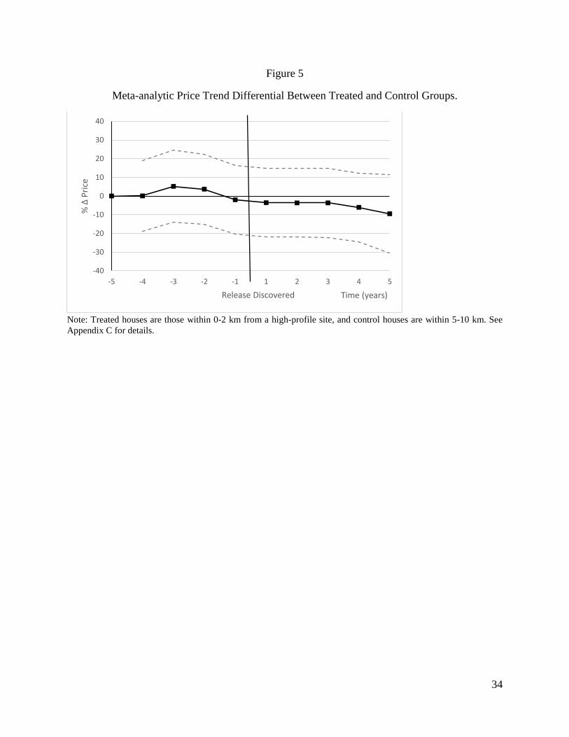
Table 2 includes descriptive statistics of all sales used in the single regression equation for

the Green Valley Citgo case. Note that the statistics only reflect data used in the regression;

specifically, of transactions of houses within 10 km of the release site, and within the five-year

period prior to the first event through the five-year period following the second event. We have

listed all variables that were used in the regressions for any of the 17 high-profile sites, even though

not all of these variables were available for this specific location.

V. RESULTS

A. Determining the Spatial Extent

We establish the appropriate spatial extent of the price effects by following an approach

similar to Linden and Rockoff (2008), and later adapted by Muehlenbachs et al., (2015). We use

local polynomial regressions to non-parametrically examine the housing price gradients around

each high-profile site before and after the most prominent milestone event. As an example,

consider again the Green Valley Citgo case in Frederick County, MD. The most prominent event

was the distribution of letters in April, 2007, notifying residents within a half mile about the

release.

To provide a clean comparison, for this exercise we narrowed the focus to sales that

occurred only two years before or after the event. We maintained the spatial limit of 10 km. To

18

further control for broader market trends over time, we first “de-trend” the prices for each site.15

The data are then separated into two groups – sales before versus after the milestone – and then

plotted against distance to the site. Two curves are fitted using local polynomial regression

techniques to depict the pre- and post-event price gradients. As shown in Figure 3 for the Green

Valley Citgo example, at greater distances the price gradients are relatively similar, suggesting

that the milestone event had little effect. However, at least in this example, we see that the prices

of houses closest to the site were noticeably lower after the event. This price differential diminishes

at around two to four kilometers.

We applied this same price gradient exercise separately to each of the 17 high-profile

releases for each site’s most prominent event, and found considerable variation in what the

appropriate spatial extent of any price effect might be.16 In all cases, however, we did not find

evidence that the price impacts extended beyond 5 km and therefore chose it as the appropriate

distance for the subsequent hedonic analyses. In order to have a representative meta-dataset, it is

important to estimate the price effects out to the same distance for all sites, even if these price

effects turn out to be zero for some sites.

B. Difference-in-Differences Diagnostics

An important diagnostic test for a DID identification strategy is to compare the price time

trends across the treated and control groups. In a valid DID quasi-experiment, such a comparison

15 The de-trended prices are calculated by estimating a simple linear regression of price on a series of year dummy

variables (with the first year omitted), and then adding the residuals back to the constant term. 16 Estimating the price gradients around just a single site and event in this fashion makes the curves potentially more

susceptible to confounding price factors that may be associated with a particular locale and time period (compared to

examining multiple sites at once, as done by Linden and Rockoff (2008) and Muehlenbachs et al. (2015), whose data

were of a single housing market, and therefore more appropriate for pooling). Nonetheless, this exercise is still

informative, and we believe such noise is reduced in the hedonic regression models, and further minimized in the

internal meta-analysis, where we do then analyze across multiple sites.

19

will show that the treatment and control groups followed relatively similar trends up to the

treatment (e.g., the discovery of a release), and then diverge after the treatment (if there is in fact

a noticeable treatment effect).

Figure 4 shows an example of these trends, for the Green Valley Citgo site. The figure

shows how residual log price varies for houses in the treatment group (those within 0-2 km from

the site, in this example) relative to the control group (houses located 5-10 km from the site), as a

function of time. In order to control for observable characteristics of the houses that were sold in

each time period, the figure is based on the residuals from a regression of log sales price on the

same set of housing-level characteristics as used in the main regression models (see section V.C),

omitting the post-milestone event variables. The figure shows the mean difference in residuals for

houses in the treatment group relative to the control group, along with an associated confidence

interval for the difference.

Overall, the figure demonstrates that the treatment and control groups have similar price

trends in the years leading up to initial detection of the release (Event 1). Despite the discovery of

a release, there is no clear difference between the two groups immediately following this milestone

event. After local residents received notification letters in 2007 (Event 2), however, prices in the

treatment group declined substantially relative to the control group.

At several sites we observed trends that are consistent with a valid quasi-experimental

interpretation of the hedonic regressions. At other sites the price trends revealed no difference, or

even a differential with a counterintuitive sign, across the treatment and control groups, suggesting

that local price trends around the site may confound the estimates of interest (see Appendix A).

We also recognize that small sample sizes in some of the distance bins may contribute to the lack

of statistical identification for some milestones (see Appendix D). In such cases, a causal

20

interpretation may not be appropriate, and so in general we caution against drawing firm

conclusions from the results for any single site.

We posit that such concerns are reduced by examining multiple sites in our subsequent

internal meta-analysis. We have no expectation a priori that the biases across sites for a treatment

effect should fall in one direction or another. Indeed, we expect that any biases are primarily

random, and are just as likely to be negative as positive. The 17 high profile sites all exist in

different property markets and the milestone events (i.e., the treatments) are spaced widely over

time. Therefore, idiosyncratic biases are reduced when estimating the average treatment effects in

our subsequent meta-analysis (Nelson and Kennedy, 2009). In addition, pooling sites in the meta-

analysis improves efficiency of our estimates by averaging across primary estimates, some of

which may not be very precisely estimated due to a small number of identifying transactions in the

initial hedonic regressions.

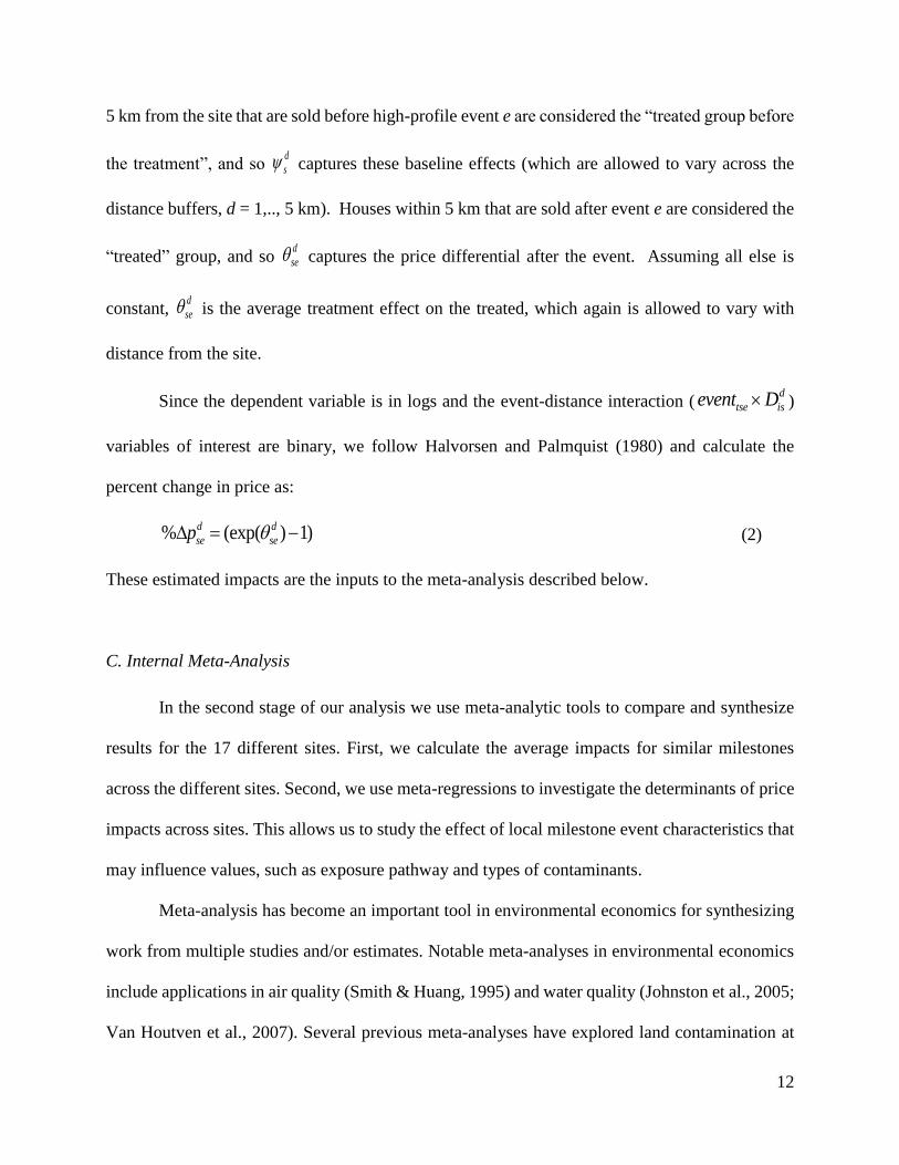
Figure 5 displays the meta-analytic counterpart to what is often referred to as an “event

analysis” (Hanna & Olivia, 2010); as it exploits the panel structure of the metadata with a treatment

(the discovery of a release in this case) occurring at different points in time. Analogous to the

previous figure that showed just one high-profile site, Figure 5 shows the price trend differential

between “treated” houses (within 0 to 2 km from a site) and “control” houses (5 to 10 km from a

site) across all 12 high-profile sites where the discovery of a release was observed.17 The

confidence intervals are fairly wide, mainly due to the small sample sizes when dividing

transactions into one year increments in the underlying hedonic regressions. Nonetheless, the trend

in the point estimates shows that the difference between the control and treated house prices are

generally zero prior to the discovery of a release, bouncing above and below the x-axis. In contrast,

17 See Appendix B for details on the derivation of this graph.

21

after the discovery of the release the points are always below the x-axis, suggesting that on average

across the sites, prices among the treated group are lower after treatment.

In short, the discovery of a release, observed at different locations across the US, and at

different times from 1980 through 2010, is followed by a decline in the price of houses in the

treated group. This is at least consistent with a causal interpretation, thus providing some evidence

that the meta-analysis as a whole is a valid quasi-experiment. We attempt to examine this price

effect more formally in the analyses discussed below.

C. Hedonic Regression Results

We estimate separate hedonic property value regressions for each study area, following

equation (1). The estimated price changes can be interpreted as relatively short-term effects, since

we only include transactions up to 5 years after the event (or less if transaction data are not

available or another high-profile event takes place sooner). The hedonic property value regressions

include census tract fixed effects, annual and quarterly time dummies, and an extensive suite of

attributes describing the housing structure, parcel, and location.18 Control variables included a

fairly consistent set of attributes across different sites. The full hedonic regression results for each

study area are presented in Appendix C.

Following equation (2), Table 3 shows the estimated percent changes in price after each

event (%Δp) for each high profile site and 1 km treatment buffer. There is noticeable heterogeneity

among the 155 estimates of %Δp, in terms of sign, magnitude, and statistical significance. This is

not surprising, given differences in distance intervals and milestone events.

18 The results of interest are robust to the inclusion of smaller census block group fixed effects, but this resulted in

larger standard errors for some sites.

22

Considering our example Green Valley Citgo site in MD, Table 3 shows that the discovery

of the release led to statistically significant declines of 3.1% and 5.5% at houses within 1 to 2 km

and 4 to 5 km, respectively, and negative but insignificant declines for the other three distance

buffers. It is surprising that the decline from the discovery of a release is so small (an insignificant

-0.4%) among houses nearest to the site (0 to 1 km). Perhaps property values at this distance

already capitalized some expectation of a future release. Just over two years later letters were sent

to residents within a half mile (or 0.8 km, roughly corresponding to our 0 to 1 km buffer), explicitly

notifying them of the release and private well contamination concerns. This “other negative”

milestone led to an additional decline in surrounding housing values; most notably a 10.1%

depreciation among houses within 0 to 1 km. The letters provided to nearby households seem to

have alleviated concerns by residents in the farthest 4 to 5 km buffer (who did not get letters), as

suggested by the positive price impact (although only marginally significant) of 4.1%.

Several other sites yield fairly intuitive results, with initial property price declines upon the

discovery of a release (e.g., the LaSalle and Jacksonville Exxon sites), and an increase in prices

after cleanup (e.g., Charnock Well Fields, LaSalle, and Northville Industries). At other sites there

are no significant effects on property values (e.g., Pearl Street Gulf), or mixed and even

counterintuitive results (e.g., Bithlo and Tuckahoe).19

To summarize and better understand the results, we more closely examine the effects of

two important and relatively common milestones. First, consider the 12 sites where we estimate

the change in price after a release is discovered. Figure 6 shows the estimated %Δp for houses in

the 0 to 1 km buffer for each site. The majority of the point estimates are negative or close to zero,

but there is a wide range, from a 27.2% decline to a 23.5% (albeit insignificant) increase. The

19 For some of these sites, such as the Bithlo site, additional caution is warranted in interpreting the results due to a

low number of identifying observations within each of the 1 km bins (see Appendix D).

23

meta-data do reveal significant heterogeneity in the price impacts of release discovery across the

different sites (χ2(11) = 237.43, p ≤ 0.000). We estimate the RES mean of the 0 to 1 km price

effects from the release discovery milestone, across all 12 relevant sites, where the grey boxes in

the figure illustrate the weights assigned to each estimate. The last line of the figure shows that the

overall RES mean is a marginally significant 4.4% depreciation (p=0.078).

Table 4 shows the RES mean effects of release discovery for each 1 km bin; the unweighted

means (where each estimate is given equal weight) are also shown for comparison, and are

generally similar (albeit a bit more sporadic, in magnitude and sometimes sign). We prefer the

RES mean estimates for the reasons discussed in section III.C.20 Similar to the 0 to 1 km buffer,

we also see a significant 4.7% average decline among houses in the 1 to 2 km buffer (p=0.038).

Beyond 2 km the discovery of a high-profile UST release has no significant effect on house values.

We emphasize that this is an average effect, and within each of the 1 km bins the meta-data suggest

statistically significant heterogeneity in the price effects across the high-profile sites (p ≤ 0.000).

At five sites the observed data allowed us to examine the price impacts after cleanup of the

UST contamination. Looking first at the 0 to 1 km buffer in Figure 7, we see that house prices

appreciated at all sites after cleanup, but the increase was only statistically significant at two sites.

Nonetheless, the overall RES mean suggests a 4.2% increase after cleanup (p=0.000). As seen in

Table 4, the unweighted mean suggests a similar average appreciation after cleanup. Interestingly,

the price effects of cleanup at the different sites seems to be relatively homogenous (χ2(4) = 2.73,

p=0.603), suggesting that the true price effect of cleaning up a high-profile release may be similar,

20 Since some of the distance buffers had a small number of observations in some of the sites, we also estimated the

means using sample size weights instead of variance. The results were quite similar to the variance weights (both in

terms of magnitude and statistical significance). For instance, the mean impact of discovery in the 0-1 km buffer was

-4.02%, and for cleanup it was 4.76%.

24

at least among houses within this closest 0 to 1 km buffer. Such homogeneity does not hold for the

more distant buffers.

The RES mean results in Table 4 show that the average increase in prices post-cleanup

extends to houses in the 1 to 2 km buffer, with an 8.7% appreciation (p=0.023). There is weak

evidence of a 4% appreciation possibly extending out to the 2 to 3 km and 3 to 4 km buffers

(p=0.118 and p=0.067, respectively), on average. In the next subsection we use meta-regression

techniques to more thoroughly examine price effect heterogeneity across the different high-profile

sites, events, and distances.

D. Meta-Regression Results

Table 5 contains the results of the main set of meta-regressions, which pool all 155

estimates of %Δp from the hedonic regressions in Table 3. The first meta-regression model

(Column 1) is an RES model following equation (3), where the moderators, or right-hand side

variables, include a separate intercept for each of the event types, following the categorization

scheme in Table 1. We also include a continuous variable denoting the different distance buffers,

for each kilometer buffer from 1 to 5. This is interacted with each of the four event type dummies

to allow the price impact gradients to differ across different types of milestone events.

Following the discovery of a release, the results suggest a marginally significant 6%

average price decrease to houses immediately adjacent to a high-profile site (i.e., distance=0). The

magnitude of this price drop diminishes with distance from the site, as suggested by the positive

(albeit insignificant) coefficient on the interaction term distance × discovered. We also see a

positive price impact from the completion of cleanup, as suggested by the marginally significant

9.3% appreciation corresponding to the dummy variable cleaned. From the negative (but again

25

insignificant) coefficient on distance × cleaned, it seems that this post-cleanup appreciation also

diminishes as distance from the site increases.

Figure 8 and Figure 9 present the full impact and significance evaluated at each distance

buffer. The figures show that, on average, the discovery of a high-profile release and its subsequent

cleanup impact property values in an intuitive fashion– prices decrease upon the discovery of a

release, but then later increase after cleanup efforts are complete. A series of Wald tests suggest

that the average post-cleanup appreciation is of an equal magnitude as the initial decrease,

suggesting that property values rebound, on average. It is important to note, however, that the

analysis is limited to property value impacts within a relatively short five-year period, and may

not capture the full property value effects over the longer-term. Further, at only three of the high-

profile sites did we observe both the discovery of a release and the completion of cleanup.

These figures also illustrate that these price effects diminish farther from the site, becoming

statistically insignificant at a distance of about three kilometers. Although we impose a linear trend

in the meta-regression specification, this is consistent with the weighted averages discussed in

section V.C, where no functional form for the distance gradient was assumed.

In Model 1, the constant and distance interaction terms corresponding to the “other

negative” and “other positive” milestones are statistically insignificant. On average, it seems that

these intermediate events do not lead to any significant impact on residential property prices.21

Our estimated price impacts generally capture the short-term effects within five years after

an event. In some cases, however, the estimates reflect an even shorter post-event time period,

21 Although not reported here, we re-estimated a restricted version of Model 1 where both positive and negative signal

events were pooled together. The resulting coefficients were insignificant and the results corresponding to release

discovery and cleanup were virtually identical to Model 1. Models restricting the price effects to be the same for

release discovery and other negative signal events, and for cleanup and other positive events were also estimated. The

resulting percent change in price estimates were all statistically insignificant when pooling events in this fashion.

26

either because later property transaction data was not yet available or because a subsequent

milestone event occurred less than five years later. The response of the housing market during

these shorter time periods may differ, or be less discernable statistically, than the response after

five full years. To examine this, the previous model is re-estimated using only observations

corresponding to the 18 milestone events (at 9 different sites) where the full 5 years of post-event

transaction data were available for the original hedonic regressions. The meta-regression results

are shown in Model 2 in Table 5. Among this subsample of sites, the discovery of a high-profile

release seems to have a larger effect on house values, suggesting a 14.4% decline for houses

immediately adjacent to the site. The price rebound from cleanup, however, is no longer

significant, but this is likely due to the fact that there was only one site where 5 years of transaction

data were available post-cleanup.

Model 3 is a Random Effect (RE) Panel regression model. This model is a recommended

alternative when more than one estimate is taken from a primary study (Nelson and Kennedy,

2009), or in our case from a high-profile release site. The RE Panel model includes a random

intercept for each high-profile site and allows the error terms to be correlated within each site. The

point estimates corresponding to the discovery of a release are very similar to the corresponding

RES model (Model 1), but are no longer significant, as illustrated in Figure 10. Model 3 also

suggests the price effects of cleanup are similar to the corresponding RES Model, although

accounting for the correlation across primary estimates yields a stronger level of statistical

significance. Model 3 even suggests a small 3.2% price increase extending out to the 3 to 4 km

buffer (see Figure 11).

A final model specification examined price effect heterogeneity across the 17 high-profile

sites. The results are not reported here, but we examined whether the price impacts varied based

27

on the exposure pathways of concern (private groundwater wells or vapor intrusion), and the

presence of MTBE contamination. MTBE is often associated with historical UST releases, and is

a challenge to clean up. Across numerous specifications focusing on the full datasets or individual

distance buffers, we found no robust evidence of price impact heterogeneity associated with the

exposure pathways or the presence of MTBE. These results suggest that benefit transfer from our

results to other high-profile UST releases, no matter the exposure pathway or presence of MTBE,

may be appropriate. This is a useful finding for policy-makers, particularly given the broad

attention previously paid to MTBE contamination.22

VI. CONCLUSION

UST releases of petroleum and hazardous substances can present risks to local residents

and the environment. This study develops monetized estimates of the benefits of cleaning up high

profile UST releases, as capitalized in local housing values. More generally, the estimated property

value effects lend insight into the value of UST release prevention, early detection, and cleanup.

A few previous studies have used hedonic methods to estimate the impacts of UST releases

on surrounding housing values (Guignet, 2013; Isakson & Ecker, 2013; Simons et al., 1997; Zabel

& Guignet, 2012), but with a narrow geographic scope. Given the abundance and broad spatial

distribution of gas stations, it is important to examine the variability in house price effects across

different locations. Identifying property value impacts of UST releases is difficult because

potential homebuyers typically have little information about nearby releases. To address this

22 For example, EPA held a Blue Ribbon Panel on the topic (http://archive.epa.gov/mtbe/web/html/action.html), and

the American Cancer Society has directed considerable resources to the study of MTBE

(http://www.cancer.org/cancer/cancercauses/othercarcinogens/pollution/mtbe).

http://archive.epa.gov/mtbe/web/html/action.html

28

challenge, our study focuses on 17 U.S. sites where high-profile UST releases were widely

publicized, involved significant community concern, and in most cases were severe.

A two-step methodology is employed, where site specific hedonic regressions are

estimated using a difference-in-differences approach for each of the 17 study areas, and then an

internal meta-analysis of the resulting hedonic estimates is conducted. Compared to highly refined

quasi-experimental property value studies (Haninger et al., 2014; Linden & Rockoff, 2008;

Muehlenbachs et al., 2015), this study was constrained by having only one (or in one case, two)

high-profile UST sites in each study area. Although great steps were taken to minimize potential

omitted variable biases, in some cases there are concerns that our single site estimates might be

susceptible to unobserved local and temporally varying influences. However, as the

aforementioned studies minimized omitted variable bias by looking at many sites within a single

housing market, our internal meta-analysis looks at many sites across the United States with release

discovery, and other milestone events occurring at different points between 1985 and 2013. To the

extent that any correlated time-variant effects are idiosyncratic across sites, this spatial and

temporal variation improves our identification of the treatment effect (Nelson, 2015), and lends

greater confidence to a causal interpretation of the estimated average price effects across all high-

profile cases.

The results suggest significant heterogeneity in the price effects across sites, but on average

show a 3% to 6% depreciation upon the discovery of a release, and a 4% to 9% appreciation after

cleanup is completed. These average effects reflect price responses within 5 years of the release or

cleanup, and diminish with distance, extending out to 2 or 3 km from the site. Since the analysis

focuses on the most high-profile UST releases, we emphasize that these results should not be

extrapolated to the broader set of more typical UST releases. Nonetheless, our findings provide

29

useful insights for assessing policies that prevent and cleanup UST releases. First, the results

demonstrate the upper reaches of cleanup benefits to nearby residents. Additionally, to the extent

that policies help prevent high-profile situations, either by preventing UST releases in the first

place or detecting them early to help minimize damages, our results may reflect closer to an

average of the avoided property value losses. Given the high number and broad distribution of

USTs across the country, the latter benefit may be quite substantial.

30

FIGURES AND TABLES

Figure 1

Locations of 17 High-Profile UST Releases

Note: Although it cannot be visually distinguished at this broad scale, the cluster of sites in Maryland actually corresponds to four

sites. Similarly, the cluster of sites in northern New Jersey and Long Island, New York consists of four sites.

31

Figure 2

Years of Transaction Data Available and Milestone Events

by Study Area

Notes: The red lines mark the timing of the high-profile milestone events examined. Case names are followed by

study area (usually county) names and for Chillum, MD a second very nearby county.

2006

2000

1992

2004

2004

2004

1990

1997

2000

2000

1996

2000

1980

1980

1980

1994

2005

2014

2013

2013

2013

2013

2011

2013

2009

2009

2009

2013

2013

2013

2013

2013

1975 1980 1985 1990 1995 2000 2005 2010 2015

Pearl Street Gulf, Chittenden, VT

Tuckahoe, Henrico, VA

Pascoag, Providence, RI

West Hempstead, Nassau, NY

Smithtown Exxon0Mobil, Suffolk, NY

Northville Industries, Suffolk, NY

Montvale, Bergen, NJ

Hendersonville Corner Pantry, Henderson, NC

Green Valley Citgo, Frederick, MD

Jacksonville Exxon, Baltimore, MD

Upper Crossroads, Harford, MD

Chillum, Prince Georges and Montgomery, MD

Palm City Cluster, Martin, FL

DeLeon Springs, Volusia

Bithlo, Orange, FL

LaSalle, Weld, CO

Charnock Well Fields, Los Angeles, CA

Year

2010

32

Figure 3

Local Polynomial Price Gradients:

Before and After “Other Negative” Milestone (Notification Letters Mailed),

Green Valley Citgo, MD

33

Figure 4

Price Trends in Treated and Control Groups at Green Valley Citgo, MD.

Note: The heavy dashed vertical line represents the initial discovery of the leak (Event 1). The lighter dashed vertical

line represents the mailing of letters to nearby residences (Event 2). Treated houses for this illustration are defined as

those within 0-2 km from the high-profile site, and control houses are within 5-10 km. See Appendix A for details.

34

Figure 5

Meta-analytic Price Trend Differential Between Treated and Control Groups.

Note: Treated houses are those within 0-2 km from a high-profile site, and control houses are within 5-10 km. See

Appendix C for details.

-40

-30

-20

-10

0

10

20

30

40

-5 -4 -3 -2 -1 1 2 3 4 5

% Δ

Pri

ce

Time (years)Release Discovered

35

Figure 6

Release Discovery: Percent changes in Price for 0 to 1 km Distance Buffer and

Random Effect Size Mean

Note: The x-axis is the percent change in price, and the estimated percent changes in price and 95% confidence intervals are shown for

each corresponding high-profile release site. The size of the grey boxes depicts the relative weights given to each observation when

calculating the Random Effect Size (RES) mean. The weights are the inverse variances of the estimates (see section III.C). The diamond

at the bottom depicts the RES mean, and the width of the diamond demonstrates the 95% confidence interval.

% Change in Price (95% CI) ID Name

36

Figure 7

Cleanup Complete: Percent Changes in Price for 0 to 1km Distance Buffer and

Random Effect Size Mean

Note: The x-axis is the percent change in price, and the estimated percent changes in price and 95% confidence intervals are shown for

each corresponding high-profile release site. The size of the grey boxes depicts the relative weights given to each observation when

calculating the Random Effect Size (RES) mean. The weights are the inverse variances of the estimates (see section III.C). The diamond

at the bottom depicts the RES mean, and the width of the diamond demonstrates the 95% confidence interval.

% Change in Price (95% CI) ID Name

37

Figure 8

Price Impact Gradient of Release Discovery: Random Effect Size Meta-Regression

(Model 1, Table 5)

Dashed lines depict 95% confidence interval.

Figure 9

Price Impact Gradient of Cleanup: Random Effect Size Meta-Regression

(Model 1, Table 5)


-14

-12

-10

-8

-6

-4

-2

0

2

4

6

0-1 1-2 2-3 3-4 4-5

% Δ

Pri

ce

Distance Buffer (km)

-5.9*-4.8*

-2.6*-1.4

-0.3

-3.7**

-10

-5

0

5

10

15

20

25

0-1 1-2 2-3 3-4 4-5

% Δ

Pri

ce


9.3*7.6**

5.9**4.2*

2.60.9

38

Figure 10

Price Impact Gradient of Release Discovery: Random Effects Panel Meta-Regression

(Model 3, Table 5)


Figure 11

Price Impact Gradient of Cleanup: Random Effects Panel Meta-Regression

(Model 3, Table 5)


-14

-12

-10

-8

-6

-4

-2

0

2

4

6

8

0-1 1-2 2-3 3-4 4-5

% Δ

Pri

ce


-5.2-4.3

-2.4-1.4 -0.4

-3.3

-4

-2

0

2

4

6

8

10

12

14

16

0-1 1-2 2-3 3-4 4-5

% Δ

Pri

ce


8.6**7.2***

5.9***4.5**

3.2**1.9

39

Table 1

Types of Milestone Events at High-Profile UST Release Sites

Event Type # of Events Examples

Release Discovered 12

Release occurred,

Previously unknown release found

Negative Signal Event

9

Previously resolved release investigation re-opened,

Additional contamination found

Positive Signal Event

5

Cleanup plans announced,

Permanent clean water supply provided

Cleanup Complete 5

Cleanup completed,

Release investigation closed and

deemed safe by regulators

TOTAL 31

40

Table 2

High-Profile UST Site Example:

Transaction Dataset Summary Statistics, Green Valley Citgo (Frederick County, MD).

Variable Obs Mean Std. Dev. Min Max

Sale price (2013$) 8,086 402,131.70 143,948.60 104,657.00 809,475.70

Age of house (years) 8,071 16.03 18.86 0 804

Age missing (dummy) 8,086 0.00 0.04 0 1

Age2 8,071 612.78 7391.64 0 646,416

Townhome (dummy) 8,086 0.21 0.41 0 1

Total # of bathrooms 8,084 2.46 0.68 0 7

Baths missing (dummy) 8,086 0.00 0.02 0 1

Interior square footage 8,084 1,921.53 732.15 672 5675

Interior sqft. missing (dummy) 8,086 0.00 0.02 0 1

Parcel acreage 8,086 0.62 1.24 0 34.7

Acres missing (dummy) NA NA NA NA NA

Air conditioning (dummy) 8,086 0.91 0.29 0 1

Air conditioning missing (dummy) NA NA NA NA NA

Basement (dummy) 8,086 0.84 0.37 0 1

Basement missing (dummy) NA NA NA NA NA

Porch (dummy) 7,212 0.91 0.28 0 1

Porch missing (dummy) 8,086 0.11 0.31 0 1

Pool (dummy) 8,086 0.02 0.15 0 1

Pool missing (dummy) NA NA NA NA NA

Distance to nearest urban cluster

(kilometers) 8,086 12.79 3.98 5.59 20.11

Located in public water service area

(dummy) 8,086 0.67 0.47 0 1

Distance to nearest major road (kilometers) 8,086 2.23 1.48 0.03 6.90

Located in 100-year flood zone (dummy) 8,086 0.00 0.05 0 1

Located on waterfront (dummy) NA NA NA NA NA

# of gas stations within 200 meters 8,086 0.00 0.06 0 1

# of gas stations within 200-500 meters 8,086 0.06 0.26 0 2

Distance to High-Profile Site (meters) 8,086 6,884 2437 65 9,999

0 to 1 km of High-Profile Site (dummy) 8,086 0.025 0.158 0 1





NA – Variable not available for Frederick County.

41

Table 3

Estimated % Change in Price After High-Profile Events.

Distance from High-Profile Site (kilometers)

Model 0 to 1 1 to 2 2 to 3 3 to 4 4 to 5 Obs.

Charnock Well Fields, CA

1 Event 1 Cleanup complete and

public well field restored

7.66*** 8.68*** 8.61*** 9.76*** 5.51** 27,598

(2.44) (2.10) (1.66) (2.50) (2.57)

La Salle, CO

2 Event 1 Leak discovered -27.20*** -33.49* -51.05*** -45.99*** -23.18*** 31,118

(4.71) (17.61) (5.99) (4.85) (8.60)

3 Event 2 Cleanup complete 7.85 80.22*** 1.96 -2.63 -11.46*** 16,334

(6.25) (18.54) (7.58) (5.03) (3.17)

Bithlo, FL

4 Event 1 Leak discovered 23.47* -2.27 21.93 27.30** 35.87** 5,383

(13.67) (28.44) (19.82) (10.86) (16.41)

5 Event 2 Widespread well

contamination, declared -2.03 50.44** 42.00** 21.64** 26.30*** 33,290

"imminent threat" (8.45) (24.75) (20.46) (10.81) (4.62)

6 Event 3 Increased notification and 35.58** 56.81** 2.72 13.50*** 2.35 8,739

media attention (14.40) (23.80) (7.63) (4.20) (7.51)

DeLeon Springs, FL

7 Event 1 Leak discovered -13.62*** 6.16 17.90*** 15.95*** 17.64* 5,971

(1.31) (6.14) (1.00) (5.97) (9.17)

8 Event 2 Cleanup approved, 21.02*** 6.48 -19.33*** -11.11* -13.74 6,036

begins year later (1.89) (4.13) (7.30) (5.97) (14.36)

Palm City Cluster, FL

9 Event 1 Leak discovered -9.90*** -78.29*** -29.54 49.80*** -1.13 20,874

(3.43) (10.70) (26.05) (13.82) (4.33)

10 Event 2 Additional contamination 6.18 30.98** -24.27* 7.26 4.87 25,949

discovered (5.33) (12.15) (12.68) (8.44) (7.55)

11 Event 3 Partially removed from -12.13*** 0.20 13.62 13.45 -0.02 21,325

"imminent threat" status (2.78) (3.15) (8.98) (19.53) (10.93)

Chillum, MD

12 Event 1 Contamination plume 0.58 2.28*** 3.75* 4.17*** 5.18*** 65,574

migrated away to DC (1.45) (0.76) (1.95) (1.12) (1.01)

Upper Crossroads, MD

13 Event 1 Leak case re-opened -4.27*** 3.01*** -0.86 4.79 1.44 4,245

(1.05) (0.79) (0.91) (3.70) (2.11)

42



14 Event 2 Public meeting and

increased well testing -1.84 -5.70*** -2.97** -2.36 -4.01 7,176

(1.35) (1.40) (1.36) (1.47) (2.90)

Jacksonville Exxon, MD

15 Event 1 Leak discovered,

emergency cleanup -14.84*** -5.17 -6.76*** -3.86* -3.84* 8,154

(1.20) (3.61) (1.03) (2.31) (2.13)


16 Event 1 Leak discovered -0.35 -3.09*** -0.35 -0.66 -5.50** 8,085

(0.71) (0.53) (3.22) (1.04) (2.19)

16 Event 2 Notification sent to all

residents within 1/2 mile -10.14*** -2.80 -1.66 -6.41*** 4.07*

(1.26) (2.72) (2.11) (1.53) (2.15)

Hendersonville Corner Pantry, NC

17 Event 1 Leak discovered 1.24 -4.38* 0.23 1.78 -4.47* 11,771

(4.01) (2.66) (7.26) (3.06) (2.35)

17 Event 2 Public water line extended -4.75 1.69 -6.03 0.52 4.58

(3.21) (6.05) (6.10) (4.49) (3.14)

Montvale, NJ

18 Event 1 Re-opened (old leak

discovered) 1.27 2.10 -5.06** 2.07 1.28 17,487

(0.89) (2.39) (2.46) (3.18) (2.66)

18 Event 2 State mandated cleanup 0.43 -4.37** -0.74 -0.56 -1.41

(0.97) (2.14) (2.01) (2.38) (2.04)

19 Event 3 Widespread vapor

concerns, RP purchased -0.58 3.55** -0.58 -7.29*** -3.06 16,452

several houses (1.23) (1.73) (2.59) (2.74) (2.92)

Northville Industries, NY

20 Event 1 Cleanup complete 3.92*** 4.36*** -0.84 3.12 0.07 34,139

(0.71) (1.09) (1.33) (2.26) (1.17)

Smithtown Exxon-Mobil, NY

20 Event 1 Leak discovered near 0.67 4.23 3.16 2.93 0.41

previous release (3.19) (3.33) (2.39) (2.95) (1.93)

20 Event 2 Cleanup complete 2.16 14.49*** 10.06*** 7.62*** 1.41

(4.21) (2.22) (2.21) (1.75) (2.11)

West Hempstead, NY

21 Event 1 MTBE detected in public 4.12** 5.38 6.08*** 2.38* 2.31** 51,945

well (2.01) (3.42) (1.61) (1.34) (1.16)

21 Event 2 New water supply well

installed

-5.84*** -2.12 -2.11 -0.30 -2.72**

(2.15) (2.64) (1.53) (1.69) (1.23)

43



Pascoag, RI

22 Event 1 Leak discovered -4.47* -13.33*** -1.04 -1.04 -9.37*** 1,786

(2.39) (2.45) (7.72) (3.44) (2.12)

Tuckahoe, VA

23 Event 1 Leak discovered 4.23** -1.08 0.52 0.02 -0.47 18,708

(1.95) (2.13) (1.67) (1.81) (1.35)

23 Event 2 Cleanup complete 4.04 -3.10** -0.20 -0.48 0.82

(3.14) (1.26) (1.56) (1.81) (1.43)

Pearl Street Gulf, VT

24 Event 1 Leak discovered -0.01 0.13 1.39 1.46 0.99 3,288

(1.74) (1.86) (2.58) (2.56) (1.50)

Note: Alternating color shades denote estimates from the same hedonic regression, as also indicated by the model number in the

first column. Estimates are derived from hedonic coefficients, based on regressions of datasets limited to transactions within 10km

of high-profile release site and sold within 5 years before or after high-profile event.

Table 4

Meta-Analysis Unweighted and RES Means

Release Discovered Cleanup Complete

Unweighted RES Unweighted RES

0 to 1 km -3.05* -4.44* 5.13*** 4.21***

1 to 2 km -10.43*** -4.72** 20.97*** 8.67**

2 to 3 km -3.13 -2.07 3.92** 4.08

3 to 4 km 4.17** 0.03 3.47*** 4.04*

4 to 5 km 0.77 -1.99 -0.74 -0.25 Note: Averages calculated using the ‘metan’ command in Stata 14. RES weights are based on the inverse variance of the estimate

(see section III.C). Unweighted means obtained using same command but equal weight given to each primary estimate.

44

Table 5

Meta-regression Base Results.

(1) (2) (3)

RES RES RE Panel

VARIABLES Model Modela Modelb

Discovered -5.99* -14.40** -5.24

(3.43) (6.76) (3.35)

Negative Event -0.43 0.28 -0.59

(4.02) (6.39) (2.37)

Positive Event 0.12 0.18 -0.79

(5.16) (6.84) (4.89)

Cleaned 9.29* 4.82 8.55**

(5.19) (14.72) (3.35)

Distance

× Discovered 1.14 3.17 0.96

(1.03) (2.04) (0.72)

× Negative Event 0.74 0.81 0.66

(1.20) (1.91) (0.55)

× Positive Event -0.41 -0.45 -0.35

(1.62) (2.13) (1.57)

× Cleaned -1.68 -0.90 -1.34*

(1.54) (4.44) (0.71)

Observations 155 90 155

# of Sites 17 9 17

Standard errors in parentheses. *** p<0.01, ** p<0.05, * p<0.1.

a. Estimated using only the 90 primary estimates corresponding to the 18 milestone

events (at 9 different sites) where 5 years of post-event transaction data were

available for the primary hedonic regressions.

b. Standard errors clustered at the high-profile site level in the Random Effects

Panel Model (Model 3).

45

WORKS CITED

ASTSWMO. (2012). Compendium of Emergency Response Actions At Underground Storage

Tank Sites: Version 1. Washington, D.C. .

Banzhaf, S. H., & McCormick, E. (2007). Moving Beyond Cleanup: Identifying the Crucibles of

Environmental Gentrification. NCEE Working Paper Series. Working Paper. US

Environmental Protection Agency. Washington, DC. Retrieved from

http://yosemite.epa.gov/ee/epa/eed.nsf/54e92d0d1f202a6885256e46007b104c/70f347d21

336d9528525725d007abf19/$FILE/2007-02.pdf

Borenstein, M., Hedges, L. V., Higgins, J. P. T., & Rothstein, H. R. (2010). A Basic Introduction

to Fixed-Effect and Random-Effect Models for Meta-analysis. Research Synthesis

Methods, 1, 97-111.

Boyle, M. A., & Kiel, K. A. (2001). A Survey of House Price Hedonic Studies of the Impact of

Environmental Externalities. Journal of Real Estate Literature, 9(2), 117-144.

Dale, L., Murdoch, J. C., Thayer, M. A., & Waddell, P. A. (1999). Do Property Values Rebound

from Environmental Stigmas? Evidence from Dallas. Land Economics, 75(2), 311-326.

Gamper-Rabindran, S., & Timmins, C. (2013). Does cleanup of hazardous waste sites raise

housing values? Evidence of spatially localized benefits. Journal of Environmental

Economics and Management, 65(3), 345-360. doi:

http://dx.doi.org/10.1016/j.jeem.2012.12.001

Gayer, T., & Kip Viscusi, W. (2002). Housing price responses to newspaper publicity of hazardous

waste sites. Resource and Energy Economics, 24(1–2), 33-51. doi:

http://dx.doi.org/10.1016/S0928-7655(01)00047-1

Greenstone, M., & Gallagher, J. (2008). Does Hazardous Waste Matter? Evidence from the

Housing Market and the Superfund Program. The Quarterly Journal of Economics, 123(3),

951-1003. doi: 10.1162/qjec.2008.123.3.951

Guignet, D. (2013). What do Property Values Really Tell Us? A Hedonic Study of Pollution from

Underground Storage Tanks. Land Economics, 89(2), 211-226.

Halvorsen, R., & Palmquist, R. (1980). The Interpretation of Dummy Variables in

Semilogarithmic Equations. The American Economic Review, 70(3), 474-475. doi:

10.2307/1805237

Haninger, K., Ma, L., & Timmins, C. (2014 ). The Value of Brownfield Remediation. NBER

Working Paper. Working Paper. National Bureau of Economic Research. Retrieved from

http://www.nber.org/papers/w20296

Hanna, R. N., & Olivia, P. (2010). The Impact of Inspections on Plant-Level Air Emissions. The

B.E. Journal of Economic Analysis & Policy, 10(1), 1-29.

Isakson, H., & Ecker, M. D. (2013). Housing Market Segmentation Around Mild Disamenities.

Technical Report. Department of Mathematics. University of Northern Iowa.

Isakson, H. R., & Ecker, M. D. (2010). The Effect of Leaking Underground Storage Tanks on the

Values of Nearby Houses.

Jenkins, R. R., Guignet, D., & Walsh, P. J. (2014). Prevention, Cleanup, and Reuse Benefits from

the Federal UST Program. National Center for Environmental Economics Working Paper.

Working Paper. Environmental Protection Agency.

Johnston, R. J., Besedin, E. Y., Iovanna, R., Miller, C. J., Wardwell, R. F., & Ranson, M. H. (2005).

Systematic Variation in Willingness to Pay for Aquatic Resource Improvements and

Implications for Benefit Transfer: A Meta-Analysis. Canadian Journal of Agricultural

http://yosemite.epa.gov/ee/epa/eed.nsf/54e92d0d1f202a6885256e46007b104c/70f347d21336d9528525725d007abf19/$FILE/2007-02.pdf

http://yosemite.epa.gov/ee/epa/eed.nsf/54e92d0d1f202a6885256e46007b104c/70f347d21336d9528525725d007abf19/$FILE/2007-02.pdf

http://dx.doi.org/10.1016/j.jeem.2012.12.001

http://dx.doi.org/10.1016/S0928-7655(01)00047-1

http://www.nber.org/papers/w20296

46

Economics/Revue canadienne d'agroeconomie, 53(2-3), 221-248. doi: 10.1111/j.1744-

7976.2005.04018.x

Kiel, K. A. (1995). Measuring the Impact of the Discovery and Cleaning of Identified Hazardous

Waste Sites on House Values. Land Economics, 71(4), 428-435.

Kiel, K. A., & Williams, M. (2007). The Impact of Superfund Sites on Local Property Values: Are

all Sites the Same? Journal of Urban Economics, 61, 170-192.

Kiel, K. A., & Williams, M. (2007). The impact of Superfund sites on local property values: Are

all sites the same? Journal of Urban Economics, 61(1), 170-192. doi:

http://dx.doi.org/10.1016/j.jue.2006.07.003

Kiel, K. A., & Zabel, J. (2001). Estimating the Economic Benefits of Cleaning Up Superfund Sites:

The Case of Woburn, Massachussetts. Journal of Real Estate Finance Economics, 22(2),

163-184.

Kohlhase, J. E. (1991). The impact of toxic waste sites on housing values. Journal of Urban

Economics, 30(1), 1-26. doi: http://dx.doi.org/10.1016/0094-1190(91)90042-6

Kuminoff, N. V., Parmeter, C. F., & Pope, J. C. (2010). Which hedonic models can we trust to

recover the marginal willingness to pay for environmental amenities? Journal of

Environmental Economics and Management, 60(3), 145-160. doi: DOI:

10.1016/j.jeem.2010.06.001

Linden, L., & Rockoff, J. E. (2008). Estimates of the Impact of Crime Risk on Property Values

from Megan's Law. American Economic Review, 98(3), 1103-1127.

McCluskey, J. J., & Rausser, G. C. (2003a). Hazardous waste sites and housing appreciation rates.

Journal of Environmental Economics and Management, 45(2), 166-176. doi: Doi:

10.1016/s0095-0696(02)00048-7

McCluskey, J. J., & Rausser, G. C. (2003b). Stigmatized Asset Values: Is It Temporary or Long-

Term? The Review of Economics and Statistics, 85(2), 276-285.

Messer, K., Schulze, W., Hackett, K., Cameron, T., & McClelland, G. (2006). Can Stigma Explain

Large Property Value Losses? The Psychology and Economics of Superfund.

Environmental and Resource Economics, 33(3), 299-324. doi: 10.1007/s10640-005-3609-

x

Michaels, R. G., & Smith, V. K. (1990). Market Segmentation and Valuaing Amenities with

Hedonic Models: The Case of Hazardous Waste Sites. Journal of Urban Economics, 28,

223-242.

Muehlenbachs, L., Spiller, E., & Timmins, C. (2015). The Housing Market Impacts of Shale Gas

Development. American Economic Review, 105(12), 3633-3659. doi: doi:

10.1257/aer.20140079

Nelson, J. (2015). Meta-analysis: Statistical Methods. In R. J. Johnston, J. Rolfe, R. S. Rosenberger

& R. Brouwer (Eds.), Benefit Transfer of Environmental and Resource Values (Vol. 14,

pp. 329-356): Springer Netherlands.

Nelson, J., & Kennedy, P. (2009). The Use (and Abuse) of Meta-Analysis in Environmental and

Natural Resource Economics: An Assessment. Environmental and Resource Economics,

42(3), 345-377. doi: 10.1007/s10640-008-9253-5

Sigman, Hilary, & Stafford, S. (2011). Management of Hazardous Waste and Contaminated Land.

Annual Review of Resource Economics, 3(1), 255-275. doi: doi:10.1146/annurev-resource-

083110-120011

http://dx.doi.org/10.1016/j.jue.2006.07.003

http://dx.doi.org/10.1016/0094-1190(91)90042-6

47

Simons, R. A., Bowen, W., & Sementelli, A. (1999). The Price and Liquidity Effects of UST Leaks

from Gas Stations on Adjacent Contaminated Property. The Appraisal Journal, 67(2), 186-

194.

Simons, R. A., Bowen, W. M., & Sementelli, A. J. (1997). The Effect of Underground Storage

Tanks on Residential Property Values in Cuyahoga County, Ohio. Journal of Real Estate

Research, 14(1/2), 29-42.

Smith, V. K., & Huang, J.-C. (1995). Can Markets Value Air Quality? A Meta-Analysis of

Hedonic Property Value Models. The Journal of Political Economy, 103(1), 209-227.

US Environmental Protection Agency. (2009). Challenges in Applying Property Value Studies to

Assess the Benefits of the Superfund Program. Office of Superfund Remediation and

Technology Innovation. US Environmental Protection Agency. Retrieved from

http://www.epa.gov/superfund/programs/recycle/pdf/PropertyStudy.pdf

US Environmental Protection Agency. (2011). FY 2011 Annual Report On The Underground

Storage Tank Program. Retrieved Dec 2, 2015, from

http://www2.epa.gov/sites/production/files/2014-

02/documents/fy11_annual_ust_report_3-12.pdf

US Environmental Protection Agency. (2014). Semiannual report of UST Performance Measures:

End Fiscal Year 2014. Retrieved April 28, 2015, from http://www.epa.gov/oust/cat/ca-

14-34.pdf

US Environmental Protection Agency. (2015). The Superfund Process. Retrieved June 16, 2015,

from http://www.epa.gov/superfund/community/process.htm

Van Houtven, G., Powers, J., & Pattanayak, S. K. (2007). Valuing Water Quality Improvements

in the United States Using Meta-Analysis: Is the Glass Half-Full of Half-Empty for

National Policy Analysis? Resource and Energy Economics, 29(3), 206-228.

Zabel, J. E., & Guignet, D. (2012). A hedonic analysis of the impact of LUST sites on house prices.

Resource and Energy Economics, 34(4), 549-564. doi:

http://dx.doi.org/10.1016/j.reseneeco.2012.05.006

http://www.epa.gov/superfund/programs/recycle/pdf/PropertyStudy.pdf

http://www2.epa.gov/sites/production/files/2014-02/documents/fy11_annual_ust_report_3-12.pdf

http://www2.epa.gov/sites/production/files/2014-02/documents/fy11_annual_ust_report_3-12.pdf

http://www.epa.gov/oust/cat/ca-14-34.pdf

http://www.epa.gov/oust/cat/ca-14-34.pdf

http://www.epa.gov/superfund/community/process.htm

http://dx.doi.org/10.1016/j.reseneeco.2012.05.006

48

APPENDICES

Appendix A: Descriptions of High-Profile Release Cases

This paper examines changes in property values near UST releases at 17 locations across the

United States (see Figure 1). Each of the 17 cases was selected because it fit the criteria for being

“high profile;” specifically, the release event was characterized by (1) media attention or

significant concern from the nearby community; (2) a major milestone such as discovery, cleanup,

or publicity within the last 15 years; and (3) close proximity to a residential neighborhood. The

objective was comprehensive spatial coverage across the contiguous United States (US). However,

sites fitting the high profile criteria tended to be located along the East Coast, and data on housing

sales were more often available for eastern states than for other US regions.

Table A-1 lists the 17 high profile release locations including community names, states, and

counties. It also identifies the source that originally suggested the case for inclusion in the study.

These sources include the federal Office of Underground Storage Tanks, EPA regional offices,

and state environmental departments, among others. Following Table A-1, we offer a concise

summary of each high profile UST release case, including details and dates surrounding the key

milestone events at the site. We begin each summary with brief statistics describing the community

in which the release occurred.

Each summary is followed by a set of graphs illustrating the price trends over the time periods

before and after the milestone events. The graphs compare houses located within 0-2 km from the

site (which we later find tends to be the extent of the average price impacts from the high-profile

UST releases and cleanups) versus houses located 5-10 km from the site (which serve as the control

groups in the main analysis). These figures show how the average residual log prices vary for

houses across the two groups. In order to control for observable characteristics of the houses that

were sold in each time period, the figures are based on the residuals from a regression of log sales

price on the same set of house and location characteristics as used in the main regression models,

including annual fixed effects (see section V.C and Appendix C); but omit the post-milestone event

variables in order to allow the price trends to vary freely over time. The figures show the mean

difference in residuals for houses in the treatment group relative to the control group, along with

an associated confidence interval for the difference.

49

Table A1: High-Profile UST Release Sites

CASE NAME STATE COMMUNITY COUNTY SITE IDENTIFIED BY

1 Charnock Well Fields CA SANTA MONICA LOS ANGELES

Office of Underground Storage Tanks:

EPA Headquarters

2 LaSalle CO LASALLE WELD EPA Region 8

3 Bithlo

FL

BITHLO ORANGE Florida Department of Environmental

Protection

4 DeLeon Springs DeLEON SPRINGS VOLUSIA

Florida Department of Environmental

Protection

5 Palm City Cluster PALM CITY MARTIN

Florida Department of Environmental

Protection

6 Chillum

MD

CHILLUM PRINCE GEORGES,

MONTGOMERY


EPA Headquarters

7 Upper Crossroads FALLSTON HARFORD


EPA Headquarters

8

Jacksonville Exxon JACKSONVILLE BALTIMORE


EPA Headquarters;

Zabel and Guignet (2012)

9 Green Valley Citgo MONROVIA FREDERICK Zabel and Guignet (2012)

10 Hendersonville Corner

Pantry NC HENDERSONVILLE HENDERSON

North Carolina Department of Environment

and Natural Resources

11 Montvale NJ MONTVALE BERGEN Web search

12 Northville Industries

NY

EAST SETAUKET SUFFOLK

New York State Department of

Environmental Conservation

13 Smithtown Exxon-Mobil SMITHTOWN

New York State Department of

Environmental Conservation

14 West Hempstead WEST HEMPSTEAD NASSAU Web search

15 Pascoag RI PASCOAG PROVIDENCE


EPA Headquarters

16 Tuckahoe VA TUCKAHOE HENRICO

Association of State and Territorial Solid Waste

Management Office (2012)

17 Pearl Street Gulf VT ESSEX JUNCTION CHITTENDEN

Association of State and Territorial Solid Waste

Management Office (2012a)

50

1. Charnock Well Fields, Santa Monica, CA

In Fall 1995, a routine water quality test by the City of Santa Monica identified the presence of

MTBE in its Charnock well fields, a groundwater source that served approximately half of the

city’s residents. By 1996, levels of MTBE between 3.1 ppb and 610 ppb were detected in 7 of the

city’s 11 wells. In response, the City shut down the contaminated wells and rerouted clean drinking

water from a neighboring supply (Lindner 2006, US DoJ 2005).

An effort to identify responsible parties for the Charnock well field contamination led to an

investigation of 30 UST sites, mostly gas stations within a mile and a half of the well fields. All

but two were associated with UST releases containing MTBE. Cleanup costs for the well field

were estimated according to one source at $200 million (US DoJ 2005, Adams 2000, Linder 2006).

Settlements were paid by up to twelve oil companies to federal EPA and to the city of Santa Monica

to compensate for past cleanup expenses. Settlement with the city was made in 2003 and was large:

$120 million. Shell, Chevron, and Exxon also signed agreements to clean the well field by building

treatment systems to remove the MTBE (Crofton 2004, US DoJ 2005). Responsible parties were

also compelled to remediate the sources of pollution (e.g., tank releases) (Linder 2006).

Santa Monica celebrated full restoration of local groundwater at Charnock and renovation of the

city water treatment plant in February 2011 (Event 1). The Charnock wells were shut due to MTBE

contamination for fifteen years (Santa Monica News Release 2011).

Santa Monica is a beachfront city located in western Los Angeles

County and abutting Los Angeles.

Population (2010): 89,736

Population density (2010): 10,664/sq mi

Median Household income (2008-2012): $72,271

Race identified as White alone (2010): 77.6%

Persons in poverty (2008-2012): 11.3%

51

Figure A1

(A) Price Trends in Treated and Control Groups at Charnock Well Fields, CA (Event 1).

(B) Difference in Price in Treated and Control Groups

Note: The gray dashed vertical line represents full restoration of local groundwater (Event 1). The figure presents

residuals from a regression of log price on a variety of control variables.

52

2. Lasalle, CO

On March 22, 2002 near the center of the town of Lasalle, Colorado employees at a bank located

just north of a combined convenience store/gas station noticed a petroleum odor and evacuated the

bank building (Event 1). Testing of the petroleum system at the adjacent store was ordered by the

state and determined that one UST was leaking unleaded gasoline at a rate of approximately 30

gallons per hour. The UST system was emptied of product. Later tests indicated the leak probably

had started in the prior month of February (Colorado Department of Labor and Employment n.d.,

Rocky Mountain News 2002).

Less than a week after March 22nd, petroleum odors were also detected at two nearby schools and

students were evacuated. Air screening tests (both indoor and outdoor) were performed at both

schools, the bank, a nearby church, and three nearby houses. Testing confirmed high levels of

petroleum vapors. Consequently, occupants of the houses and buildings were evacuated.

Remediation involved soil vapor extraction wells and ground water pump and treat systems

(Colorado Department of Labor and Employment). The schools were evacuated for 12 to 18 days

(Cornelius 2002). The Denver Post reported:

“This is a big deal because we have people who can't conduct business, people who can't

live in their homes, people who can't go to school. This is an emergency," said Eric

Gillespie, an environmental protection specialist with the Colorado Division of Oil and

Public Safety” (Cornelius 2002).

By late March 2002, remediation had resulted in the recovery of approximately 38,000 gallons of

ground water and 4,000 gallons of free-phase product. Vapor was monitored in several

houses/buildings from 2002 to 2006. In September 2009 the groundwater results along with the

clean soil confirmation allowed for event closure (Event 2) (Colorado Department of Labor and

Employment).

Lasalle is a small town in Weld County in northeast Colorado,

about an hour from Denver, consisting of less than one square mile.






53

Figure A2

(A) Price Trends in Treated and Control Groups at Lasalle, CO (Event 1).


Note: The heavy dashed vertical line represents the initial discovery of the leak (Event 1). The figure presents residuals

from a regression of log price on a variety of control variables.

54

Figure A3

(A) Price Trends in Treated and Control Groups at Lasalle, CO (Event 2)


Note: The heavy dashed vertical line represents event closure for the leak (Event 2). The figure presents residuals


55

3. Bithlo, FL

All 8,000 plus residents of Bithlo, Florida as recently as 2011 relied on groundwater for drinking

water. The town is host to a notorious persistent gasoline release at a local gas station. Leaking

gasoline was reported as early as November 1988 (Event 1) when a determination was made that

a large number of affected houses warranted further assessment and cleanup (Roe 2012).

Contamination from the same gas station continued as recently as November 2011 when the press

reported that the source had contaminated water for thousands of Bithlo residents. The press also

reported about other sources of groundwater contamination including an old recycling center

(WFTV 2011)

From 1999 to 2000, monitoring wells were installed and have been in place through the present

time (Oculus 2015). In April 2003, Bithlo was deemed in “imminent threat status” (Event 2) due

to widespread contamination of potable wells (Roe 2012 citing Water Supply Analysis 2011).

Following letters being sent to homeowners regarding well water testing in November 2011 (Event

3), press and community meetings were prolific in the 2011 to 2012 period as the community

discussed whether to connect to state water lines. However, Bithlo has a high poverty rate and

residents have reportedly resisted public water due to the expense (WFTV 2011).

In 2012, the groundwater remediation was continuing at the leaking UST site in Bithlo. Also the

responsible party or the state had supplied water filtration units to a total of 24 houses. However,

potable wells at 17 houses or other places in Bithlo had been identified as not having a filter and

exceeding the Maximum Contaminant Level (MCL) for petroleum constituents (Roe 2012).

Bithlo consists of about 10 square miles in Orange County. Bithlo

is located approximately 20 miles east of Orlando and 20 miles

west of the coast.


Population density (2010): 770.3/sq mi




56

Figure A4

(A) Price Trends in Treated and Control Groups at Bithlo, FL (Event 1).


Note: The heavy dashed vertical line represents the discovery of the leak (Event 1). The figure presents residuals from

a regression of log price on a variety of control variables.

57

Figure A5



Note: The dashed vertical line represents the imminent threat determination (Event 2). The figure presents residuals


58

FigureA6



Note: The dashed vertical line represents letters sent to homeowners (Event 3). The figure presents residuals from a

regression of log price on a variety of control variables.

59

4. DeLeon Springs, FL

In June of 1985, residential neighbors to a gas station located downtown DeLeon Springs, Florida

reported gasoline in their drinking well (Event 1). About a year later, free product was detected by

a monitoring well at the gas station. A remedial action plan was approved on August 29, 1990 and

groundwater cleanup began soon after (Event 2). Cleanup activities have continued off-and-on

since then. Remediation has proven difficult and lengthy, attributed in part to high permeability of

the soil, and in part to the plume spreading beneath an adjacent highway. An initial pump and treat

remedial system was subsequently abandoned as ineffective (Pulver 2014, Universal Solutions,

Inc 2005).

Given that the town grew up around natural springs, it is not surprising that at least some, and

perhaps many, residents of DeLeon Springs relied on groundwater when the gasoline release

occurred. Thus the contamination plume posed risks to human health. An elementary school

discovered gasoline constituents in its seldom-used well. Residents were provided with bottled

water, well filtration systems, and deeper wells (Tonyan 1987, Andrews 2011). The gasoline

release has been blamed by residents as preventing economic development in the town center

(Andrews 2012).

In approximately 2011, the plume was described by the press as moving towards the De Leon

Springs State Park. However, in response to cleanup activity, by 2014 the plume had diminished

in size. In April 2014 a new remediation effort began that included removing the highway surface

and cleaning the soil underneath. The cleanup at DeLeon Springs is one of the 10 most expensive

addressing UST releases in Florida (Pulver 2014).

Natural springs attracted settlers in the 1800s to DeLeon Springs. The

current town is about 2.5 square miles, located 30 miles inland from

Daytona Beach, and hosts DeLeon Springs State Park. It is located in

Volusia County.






60

Figure A7

(A) Price Trends in Treated and Control Groups at DeLeon Springs, FL (Event 1).


Note: The heavy dashed vertical line represents the initial discovery of gasoline in drinking water (Event 1). The

figure presents residuals from a regression of log price on a variety of control variables. For details, refer to Figure 4

in the main text.

61

Figure A8

(A) Price Trends in Treated and Control Groups at DeLeon Springs, FL (Event 2).


Note: The dashed vertical line represents initiation of groundwater cleanup (Event 2). The figure presents residuals


62

5. Palm City Cluster, FL

This event involves UST releases at three gas stations located near one another along a highway

in Palm City, Florida (Tyko 2006, Oculus 2013). The releases were discovered in 1988 (Event 1)

and initial testing of nearby wells identified a handful as contaminated with benzene and/or MTBE

(Sorentrue 2003).

When the county was installing new water and sewer lines in October 1996, two plumes of

petrochemicals were discovered (Event 2) (Andreassi 2001). Fears were expressed that the nearby

St. Lucie River was threatened. Well testing accelerated in 1996 with calls by the local population

for investigations. Indeed, over the entire period between 1991 and 1998, USTs were removed and

contaminated soil was excavated (Sorentrue 2003). In 2001, an extraction system was installed to

remove contamination from groundwater (Andreassi 2001). Nevertheless, the plume traveled over

the years, accelerated in part by draws on the groundwater by drinking wells, and by 2003 at least

58 residential wells had been identified as contaminated (Sorentrue 2003).

Florida Department of Environmental Protect (DEP) paid to connect some, but not all, of these

houses to public water sources. Many of the houses were rental properties, which was highlighted

by the press as one reason for slow progress. By 2003, a total of 24 houses and businesses had

been connected to the public water system. The goal of state and local government was to connect

another 241 (Sorentrue 2003).

The most recent cleanup activity was completed in 2012 although there is one release still subject

to ongoing remediation. Two of the three releases were removed by the Florida DEP from

“imminent threat status” in 2008 (Event 3). The third was removed in 2011 (Oculus 2013).

Palm City is part of the Port St. Lucie metropolitan statistical area on the east

coast of Florida. It consists of about 16.5 total square miles including 2 square

miles of water in Martin County.






63

Figure 12

(A) Price Trends in Treated and Control Groups at Palm City Cluster, FL (Event 1).




64

Figure A10



Note: The dashed vertical line represents the discovery of new plumes (Event 2). The figure presents residuals from


65

Figure A11



Note: The light dashed vertical line represents removal from imminent threat status (Event 3). The figure presents


66

6. Chillum, MD

In 1989, there was a reported release of an unknown amount of gasoline from an underground

storage tank at a service station located in Chillum, Maryland (US EPA Region 3 2008). The

release was initially addressed by the Maryland Department of the Environment (MDE). MDE

required owners of the gas station to install a pump and treat system to remove the gasoline from

the ground water. That system has been in operation since 1990 (Neibauer 2012).

In April 2001, the gasoline plume was reported to have migrated into the District of Columbia

(Event 1), underlying a residential area just south of the Washington D.C. boundary (US EPA

Region 3 2008). Subsequent investigation revealed that perchloroethylene was also present in

groundwater at elevated concentrations. At least one news story suggested this chemical could be

associated with a nearby dry cleaner (Santana 2004).

In October 2001, a DC Councilmember (Fenty) asked EPA to assume responsibility for the

gasoline release investigation (Santana 2004). EPA’s cleanup decision consisted of continued

operation of the groundwater remediation (pump and treat) system operating in Maryland. The

system was expanded by installing additional wells set at angles to recover contaminated water

from the Washington DC neighborhoods. EPA noted that the drinking water for the area was not

at risk as its source was a public drinking water supply and not the local groundwater (US EPA

Region 3 2008). Air contamination was an issue. Individual vapor mitigation systems were

installed in houses located above the gasoline plume where petroleum vapor concentrations

exceeded EPA indoor air standards. Work on the vapor mitigation was completed by early 2009

(US EPA Region 3 2009).

In addition to the precautions above, EPA responded to public comments by strengthening the

remediation plan by, for example, adding an independent remedial system to the Washington DC

area (US EPA Region 3 2008). An Administrative Order of Consent to implement the final remedy

became effective in early 2009 (US EPA Region 3 2015). Cleanup of the plume began soon after

and construction of the final remedy was completed in the summer of 2013 and will run for

approximately a decade (Fan 2013).

Chillum is a densely populated suburb located in Prince Georges County

Maryland and bordering Montgomery County, Maryland and Washington, D.C.

It is predominantly African American and consists of four neighborhoods.






67

Figure A12

(A) Price Trends in Treated and Control Groups at Chillum, MD (Event 1).


Note: The heavy dashed vertical line represents gasoline plume migration into D.C. (Event 1). The figure presents


68

7. Upper Crossroads, Fallston, MD

In 1990, MTBE was discovered in drinking water wells at a Fallston, Maryland gas station and

several other nearby commercial establishments. The most contaminated well was at the gas

station, where the MTBE level was just below the state action level. The discovery was an outcome

of proactive testing of wells located near gas stations by the county health department. As a result

of the discovery, monitoring wells near the UST system were installed and they detected MTBE

at levels below the State action level. In May 1993, the level was non-detectable. As a result, the

MDE closed the investigation (Maryland Department of Environment 2006).

In December 1998, the health department well tests in Fallston turned up MTBE contamination

above state action levels at a nearby restaurant (Event 1), which subsequently closed for unrelated

reasons. Routine testing again turned up elevated MTBE at a commercial facility near the original

gas station in 2000. At that point, MDE required the station’s owners to purchase a filtration system

for the affected facility and to conduct more extensive subsurface testing to determine the location

and extent of the MTBE contamination plume (Maryland Department of Environment 2006,

2010).

The results of the gas station’s subsurface investigation were reported in 2003 and led to further

testing at off-site wells. By spring 2004, many residential wells were found to have trace amounts

of MTBE, and one was discovered with triple state action levels. In June 2004 MDE sent letters

notifying impacted residents, followed by a public meeting on June 21, 2004 (Event 2), and a

subsequent increase in public communication. This led to still more testing and, before the end of

2004, installation of a remediation technology to collect and treat vapors from the soil around the

UST system. At least ten affected houses received a well water filtration system (Maryland

Department of Environment 2006, Wheeler 2004). The community expressed outrage in 2004 that

they were just learning about contamination detected from a source as early as 1991 (Wheeler

2004). By 2005, the case was associated with 225 residential wells with trace amounts of MTBE;

11 wells contaminated above the state action level; and two class action lawsuits (Mitchell 2005).

Fallston is a semi-rural community or an “exurb” located a bit under 30

miles Northeast of Baltimore in Harford County. It is 14 square miles of

farms and suburban development and one shopping/business district.






69

In April 2005, the gas station permanently closed. The company reported the cause as nearby

roadwork and bad publicity due to the contamination (Mitchell 2005). Between April 2006 and

June 2008, a pump- and-treat remediation system was in place that recovered and treated

groundwater and vapors at the closed station. Then the system was turned off to allow groundwater

to return to historic baseline levels. In May 2010, historic groundwater levels had returned and

samples taken from almost 100 shallow, intermediate, and deep monitoring wells confirmed that

MTBE contamination was greatly reduced from 2005 levels and in all but 1 of the 100 wells was

below actionable levels. The MDE approved permanent shut-down of the pump and treat system

and commencement of post-remedial monitoring (Maryland Department of Environment 2010).

70

Figure A13

(A) Price Trends in Treated and Control Groups at Upper Crossroads, Fallston, MD (Event 1).


Note: The heavy dashed vertical line represents the discovery of MTBE (Event 1). The figure presents residuals from


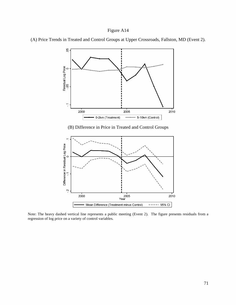
71

Figure A14

(A) Price Trends in Treated and Control Groups at Upper Crossroads, Fallston, MD (Event 2).


Note: The heavy dashed vertical line represents a public meeting (Event 2). The figure presents residuals from a


72

8. Jacksonville Exxon, MD

A major petroleum release from a gas station UST system product line in Jacksonville, Maryland

was reported to the MDE in Jacksonville on February 17, 2006 (Event 1). Gasoline 15 feet deep

was measured at an on-site monitoring well nearest the underground tanks, and gasoline 8 feet

deep was measured at another. The state immediately shared information about the release with

both the county department of environment and the community association. By the next day, all

tanks at the station had been emptied and the station was closed (Maryland Department of

Environment 2008).

Close study of inventory records suggested that over 25,000 gallons of unleaded gasoline had been

released over an approximately one-month period. Recovery wells were installed on site and

monitoring wells were installed at surrounding properties. Vapor was monitored as were nearby

streams. Over the course of the incident, gasoline was never detected in surface water or in storm

water outflows (Maryland Department of Environment 2008).

It did, however, contaminate subsurface soil and groundwater. Over 250 drinking water wells were

tested and were still sampled regularly as of 2014 (Maryland Department of Environment 2014b).

Either as a precaution or because water samples exceeded contamination standards for MTBE,

BTEX, or benzene, filtration systems were installed on wells at 13 houses by September 2008.

Some houses also were monitored for vapor intrusion (Maryland Department of Environment

2008). Two court cases were brought against the gas station owners in Jacksonville and gained

prominence in part because of the extent of damages awarded. In one case involving over 160

households and businesses, damages of approximately $1.5 billion were awarded, though the

largest award of $1 billion in punitive damages was subsequently revoked by an appeals court. In

the second case, 84 households were awarded almost $150 million, also later rejected by an appeals

court (Hirsch 2013).

Jacksonville itself is not a census designated place, however it is part of the

Phoenix, MD zip code area. Phoenix consists of 22 square miles and is

located 20 miles north of Baltimore in Baltimore County. The following

statistics are for Phoenix.






73

By 2008, almost 11,000 gallons of liquid gasoline had been recovered, and additional gasoline was

collected in vapor or dissolved form. Groundwater was being pumped and treated at 78 wells, and

monitored at 262 (Maryland Department of Environment 2008). Indeed as of the present time, soil

vapor extraction and groundwater pump and treat remediation continues (Maryland Department

of Environment 2014).

Figure A15

(A) Price Trends in Treated and Control Groups at Jacksonville Exxon, MD (Event 1).


Note: The heavy dashed vertical line represents the release of petroleum (Event 1). The figure presents residuals from


74

9. Green Valley Citgo, Monrovia, MD

In December 2004, the MDE discovered MTBE contamination in the drinking water supply

well that serviced a shopping center in Monrovia, Maryland (Event 1). Inspection of a nearby gas

station led to drilling of new monitoring wells and in February 2006, MTBE and benzene were

detected above state action levels at one of the monitoring wells. Later that same year, MTBE was

detected at a nearby plaza above state action levels. Subsequent quarterly sampling of the wells at

the plaza and the shopping center identified increasing MTBE levels between 2007 and early 2008.

As a consequence, one supply well was closed and filtration systems were installed at several

others (Maryland Department of Environment 2010b).

The nearby residential population also depended on groundwater for drinking water. In April

2007, the health department under directive from MDE sent letters to nearby residents within a

half mile of the gas station (Event 2) notifying them of MTBE contamination issues (Maryland

Department of Environment 2010b). The UST system and petroleum contaminated soil were

removed in the summer of 2008 and a new system constructed of higher quality materials was

installed. A treatment system was placed at the nearby stormwater discharge (Maryland

Department of Environment 2010b).

By April 2010, 239 private drinking water wells had been sampled. Six were identified with

MTBE at greater than state action levels and each received filtration systems and regular

subsequent monitoring. The wells at an additional 23 residences near the six affected houses

received quarterly groundwater monitoring (Maryland Department of Environment 2010b), as did

the nearby plaza and shopping center as of 2014 (Maryland Department of Environment 2014c).

As of 2015, filtration systems remain in effect at these impacted supply wells. The case remains

open, natural attenuation and ongoing monitoring in place (MDE, 2015).

A large lawsuit for $3.75 billion was filed by 75 plaintiffs near the contamination in early 2010

(Lecke 2010). The case reached a confidential settlement in spring 2014 (Gaines 2014). The gas

station continued to operate as late as 2014 (Maryland Department of Environment 2014c).

Monrovia is a very small community in Frederick County

located almost equidistant (about 45 miles) from Baltimore and

Washington DC.

Population (2010): 416

Population density (2010): 186/sq mi

Median Household income (2012): $80,765



75

Figure A16

(A) Price Trends in Treated and Control Groups at Green Valley Citgo, MD (Event 1).


Note: The heavy dashed vertical line represents discovery (Event 1). The light dashed vertical line represents letters

(Event 2). The figure shows residuals from a regression of log price on controls.

76

10. Corner Pantry, Hendersonville, NC

In April 2003, in anticipation of selling the property, an environmental assessment of a

Hendersonville gas station discovered soil contaminated with gasoline constituents (Event 1).

Months later, while drilling a new well, a nearby homeowner discovered groundwater with a

petroleum odor. The water was tested and MTBE and other gasoline chemicals were detected.

Further testing of wells in the area turned up high levels of MTBE. The source was traced to the

UST system at the gas station (North Carolina Department of Environment and Natural Resources

2004).

By late 2003, approximately 60 private wells had been sampled and community wells that served

dozens of nearby houses had been found tainted with MTBE and benzene (North Carolina

Department of Environment and Natural Resources 2004, Metzger 2005). According to a state

official, among drinking water contamination sites, this one became the state’s top priority. The

reason was the large number of vulnerable drinking water wells, one of which provided water to

an assisted living facility. The cleanup involved vapor collection and treatment and moved forward

despite a large backlog of releases and scarcity of cleanup funds in the state (Metzger 2003, 2005).

To quickly address contaminated drinking water, filtration systems were installed or alternative

sources of water provided, such as hookups to alternative clean wells, or provision of bottled water

(North Carolina Department of Environment and Natural Resources 2004). By July 2005, water

lines were extended by the city to almost 100 houses with contaminated wells or considered at risk

(Event 2) (Metzger 2005).

Hendersonville is located about 20 miles south of Asheville and 100 miles west of

Charlotte in Henderson County. It consists of 7 square miles at the southern edge of

the Blue Ridge Mountains.


Population density (2010): 1,892.9/sq mi

Median Household income (2009-2013): $ 37,060


Persons in poverty (2009-2013): 26%

77

Figure A17

(A) Price Trends in Treated and Control Groups at Hendersonville Corner Pantry, NC (Event 1).


Note: The heavy dashed vertical line represents the initial discovery of the leak (Event 1). The light dashed vertical

line represents extension of city water (Event 2). The figure presents residuals from a regression of log price on a

variety of control variables.

78

11. Montvale, NJ

A slow gasoline release at a gas station in Montvale, New Jersey seeped into groundwater over

approximately 10 years. The New Jersey Department of Environmental Protection (NJDEP) first

learned of potential contamination at the site in 1988 when there was a surface release from a hose

that had been clipped by suspected vandals. At that point, it ordered commencement of monitoring.

However, according to gas station records, soil contamination was first discovered by monitoring

wells installed in 1983. Then in August 1993, while removing old USTs, the station owner

discovered that three of them had been leaking (Event 1). The tanks were replaced with higher

quality USTs and the state was notified of contamination. Soil sampling and installation of

additional monitoring wells were required (Holahan 2003, 2004).

The NJDEP mandated cleanup in February 1996, including vapor extraction (Event 2). In June

2002, a pump and treat system began cleaning polluted groundwater and additional monitoring

wells are installed to better assess the severity and extent of contamination (Event 3). This was

followed by air sampling of nearby houses, which subsequently led the gas station owner to

purchase five impacted houses (Holahan 2003).

In 2004, more than a dozen houses were being monitored for soil and air contamination. The

drinking water was not compromised, perhaps because the nearby houses were not using

groundwater. Homeowners reported to the press and filed a law suit claiming that house values

had dropped precipitously (Holahan 2004).

Remedial activities continued as late as 2012 (NJ DEP 2012).

Montvale was incorporated as a borough in 1894 and is named for its

topography (Montvale, NJ n.d.). It is located along the northern border of

New Jersey in Bergen County abutting New York State.



Median Household income (2009-2013): $ 107,662



79

Figure A18

(A) Price Trends in Treated and Control Groups at Montvale, NJ (Events 1 and 2).



line represents NJDEP mandating cleanup (Event 2). The figure presents residuals from a regression of log price on a


80

Figure A19

(A) Price Trends in Treated and Control Groups at Montvale, NJ (Event 3).


Note: The heavy dashed vertical line represents installation of a pump and treat system (Event 3). The figure presents


81

12. Northville Industries, East Setauket, NY

A gasoline release was discovered at a petroleum storage, distribution and wholesale facility in

East Setauket, New York in November of 1987. A small hole in an underground pipeline was

uncovered while the firm was installing a groundwater monitoring well. Gasoline had spread over

30 acres and reached the water table, 100 feet down. The facility notified the state and estimated

that 1.2 million gallons of gasoline had leaked over the past decade (Schmitt 1990, New York State

Department of Environmental Conservation 2006). A New York Times article in 1990 declared

that since discovery of the release

“…Robin Hood Lane, the quiet residential street that is the gasoline plume's western

boundary, has become the front line of what experts say will be a decade long experiment

in combining various kinds of technology to clean up one of the worst underground spills

in the New York metropolitan region.” (Schmitt 1990)

In 1989, before recovery operations began, soil vapor monitoring identified two houses

contaminated with petroleum-related compounds. These houses were remediated and no soil

vapors were detected in houses at levels that would harm human health subsequent to 1993 (New

York State Department of Environmental Conservation 2006).

Owners of the petroleum storage facility funded connection to the county water supply for all areas

nearby that had not previously received public water. The public well fields were closely

monitored and none were found contaminated (New York State Department of Environmental

Conservation 2006).

The owners investigated the full extent of contamination which involved installation of more than

300 wells within and surrounding the area of contamination. Soil vapor monitoring occurred at

over 100 vapor monitoring wells; groundwater monitoring at over 200. In 1994, the facility

reached agreement with the state on plans to remediate the soil and groundwater contamination. A

vapor extraction system operated until 2004. Other components of the cleanup included an air

sparging system which operated intermittently until 2003, and groundwater extraction and

East Setauket is not itself a census designated place but is part of the Setauket

CDP, a community founded in the mid-17th century. It is located on the northern

shore of Long Island in Suffolk County, about 60 miles from Manhattan.






82

treatment which took place until 2000 (East Setauket 2005; New York State Department of

Environmental Conservation 2006). Initial plans were to build a groundwater filtration plant that

could treat more than 3.5 million gallons of water each day (Schmitt 1990).

Cleanup and remedial work required by the state was successfully completed as of November 2006

(Event 1). Deconstruction and abandonment of monitoring wells, recovery wells and other

buildings and structures associated with the cleanup began and were expected to be completed in

approximately four months (Sobel 2006).

83

Figure A20

(A) Price Trends in Treated and Control Groups at Northville Industries, NY (Event 1).


Note: The light dashed vertical line represents completion of cleanup (Event 1). The figure presents residuals from a


84

13. Exxon-Mobil, Smithtown, NY

A spill of an unknown quantity of gasoline occurred at a Smithtown, New York gas station in

September of 1998 (Vargas 2004). A local resident suspected that her drinking well was

contaminated. The county health services confirmed that the well contained levels of MTBE that

exceeded regulatory standards. Alternative drinking water was provided to the household. The

New York State Department of Environmental Conservation (NYSDEC) began an investigation

seeking to identify other affected residences and supply them with alternative drinking water

(ExxonMobil Oil Corp 2010). A cleanup ensued that removed a tank and 5,000 tons of

contaminated soil near the station before the end of 1999 (Allison 2008, Groundwater &

Environmental Services, Inc. 2012).

In March 2004, NYSDEC reported a gasoline release near the 1998 incident but across the street,

at a second gas station in Smithtown (Event 1). At least some residents stated they were unaware

of any release until this second incident. (Vargas 2004). In July of 2004, individuals from seventy-

two households in the path of the release plume sued the gas station owners for damages (Allison

2008).

A groundwater pump and treat system operated between June 1999 and June 2007 and a soil vapor

extraction system operated from April 2001 to March 2006. Groundwater monitoring was ongoing

as late as November 2010, and an off-site pump and treat system operated between 2004 and 2010

(ExxonMobil Oil Corp 2010, Groundwater & Environmental Services, Inc. 2012). Except for

ongoing monitoring, cleanup activities seem to be complete by January 2010 (Event 2).

Smithtown CDP lies within the boundaries of the town of Smithtown in

Suffolk County. The CDP consists of 12 square miles, while the town consists

of 111 square miles split almost evenly between land and water. Smithtown is

on the northern coast of central Long Island. The town was settled in the mid-

17th century and is about 50 miles from Manhattan.






85

Figure A21

(A) Price Trends in Treated and Control Groups at Smithtown Exxon-Mobil, NY

(Events 1 and 2).



line represents the completion of cleanup (Event 2). The figure presents residuals from a regression of log price on a


86

14. West Hempstead, NY

In June of 2006, MTBE was detected at concentrations exceeding the state standard in the West

Hempstead (New York) Water District distribution system (Event 1). The contamination infiltrated

through a public supply well, one of four relatively shallow wells. A precautionary health advisory

warned approximately 30,000 customers not to ingest or wash with the tap water. All four wells

were closed pending further investigation by the NYSDEC exploring the source, extent, and degree

of the contamination (New York State Department of Environmental Conservation 2007, Smith

2007, Three Village Times 2006, White 2006). Ultimately the four wells were found to be

contaminated (New York State Comptroller 2007).

Beginning in August 2006, a pump and treat system was installed to clean water from the

contaminated well. By early 2007, the contaminant plume had been delineated. Besides MTBE,

tert-amyl-methyl-eter and tert-butyl-alcohol were also detected. Only the shallow aquifer was

affected so public wells drawing from a deeper aquifer were considered safe. Also in early 2007,

a second remedial measure was started consisting of new recovery wells that pumped and treated

water from the contaminated plume. Both remedial measures were expected to operate for two to

three years. A gas station located about one mile north of the public wells was identified as a

source of the contamination, possibly sharing responsibility with other sources. (New York State

Department of Environmental Conservation 2007, Smith 2007).

A new drinking water supply well was installed at an alternative location. The new source was put

into service in June 2007 (Event 2) (New York State Comptroller 2007).

West Hempstead CDP is located on the western portion of Long Island,

about 25 miles from Manhattan. It occupies 2.5 square miles in Nassau

County and is host to a portion of Hempstead Lake State Park.






87

Figure A22

(A) Price Trends in Treated and Control Groups at West Hempstead, NY (Events 1 and 2).



line represents installation of a drinking water supply well (Event 2). The figure presents residuals from a regression

of log price on a variety of control variables.

88

15. Pascoag, RI

High levels of MTBE were discovered in a public-supply drinking water well field that served

Pascoag Village, Rhode Island in August 2001 (Event 1), just a few months after a new well had

been activated. The state health department issued an order to limit exposure to the well water on

September 4, 2001. Over the next 3 months, several health advisories were issued and the levels

of MTBE detected kept rising. More than 4,000 residents received deliveries of bottled water for

several months. The Burrillville School District provided access to water for showering and filling

water jugs at a hockey rink. The public wells were shut down in January 2002. The contamination

was traced to leaking tanks at a very nearby gas station (Schweisberg 2005, Allen and Boving

2006, Fisher 2011, Fitzgerald 2012).

The UST system release occurred only 1700 feet from the public water supply wellhead. Prior to

the release event, the source had been identified as a relatively high risk point source of

contamination within a designated protection zone surrounding the wellhead. The source had been

inspected just months before the contamination was discovered in the water supply (Schweisberg

2005).

During the emergency investigation, at some wells over 6 inches of gasoline was discovered.

Vapors intruded a nearby house for the elderly and caused a temporary evacuation. Contamination

was consistently detected in the nearby Pascoag River (Allen and Boving 2006).

Eventually, public water was provided to Pascoag residents from a neighboring district

(Schweisberg 2005, Fisher 2011). However, new drinking water wells closer to house were being

sought as late as 2012 (Fitzgerald 2010).

1,300 homeowners were involved in a suit against the gas station which settled for $7 million in

2012; $2 million for residents and $5 million to Pascoag’s Public Utility for cleanup costs and

The Pascoag CDP is the principal village (out of seven villages) in

the town of Burrillville, RI. The village consists of 5.5 square miles

and is centered around the Pascoag River and Reservoir (Pascoag,

Rhode Island). It is about 25 miles from Providence.


Population density (2010): 832/sq mi




89

supplying alternative sources of water. The latter were supplied through new wells and pipelines

to connect houses that relied on private wells to public sources. Cleanup activities included soil

removal, installation of filtration units, and pumping groundwater (Fitzgerald 2012).

Figure A23

(A) Price Trends in Treated and Control Groups at Pascoag, RI (Event 1).




90

16. Tuckahoe, VA

In early 2010, new owners of a Tuckahoe gas station hired contractors to install new line leak

detectors for an existing fiberglass tank system. Approximately one week later, on March 4, a

release was reported (Event 1) to the Virginia Department of Environmental Quality (VDEQ).

Inventory reconciliation suggested that about 15,000 gallons of gasoline had been released. The

contractor took responsibility for the release which was attributed to faulty installation

(Association of State and Territorial Solid Waste Management Office 2014, Springston 2010).

The gasoline seeped into a nearby creek, through soil and a concrete culvert. The cleanup effort

included protecting the creek with booms and other devices intended to prevent the spread of

gasoline into water. Vacuum extraction was employed from the tank pit and wells near the creek.

Vacuum operations ended and soon after, explosive levels of vapors were detected in the sewer

lines near the station. In addition, a restaurant almost one mile away reported gasoline vapors in

their floor drains (Association of State and Territorial Solid Waste Management Office 2014).

Public water supplies were not threatened (Jenks 2010).

VDEQ and EPA delineated the boundaries of the vapor movement through sewer lines. The sewer

system led to a nearby residential neighborhood and other businesses, all of which faced risks of

vapor intrusion. Surfactant was fed into the tank pits to suppress the vapors. Blowers were installed

in sewer manholes located between the gas station and the neighborhood. Vacuum truck recovery

of product from the tank pit was reinstated and an extraction unit was eventually installed for 24-

hour operation. Finally, the county initiated a lining project for the nearby sanitary sewer line for

protection from possible future releases. Over 11,000 gallons of gasoline were recovered during

the first two weeks of cleanup (Association of State and Territorial Solid Waste Management

Office 2014). By the end of the two weeks, VDEQ reported that while there were complaints of

gasoline odors during the initial days, there had been no recent complaints (Springston 2010).

Tuckahoe CDP is a close-in north-western suburb of Richmond; in fact,

the mailing address is Richmond. It consists of about 20 square miles in

Henrico County. The Western boundary of Tuckahoe is formed by a

large undeveloped swampy creek of the same name.






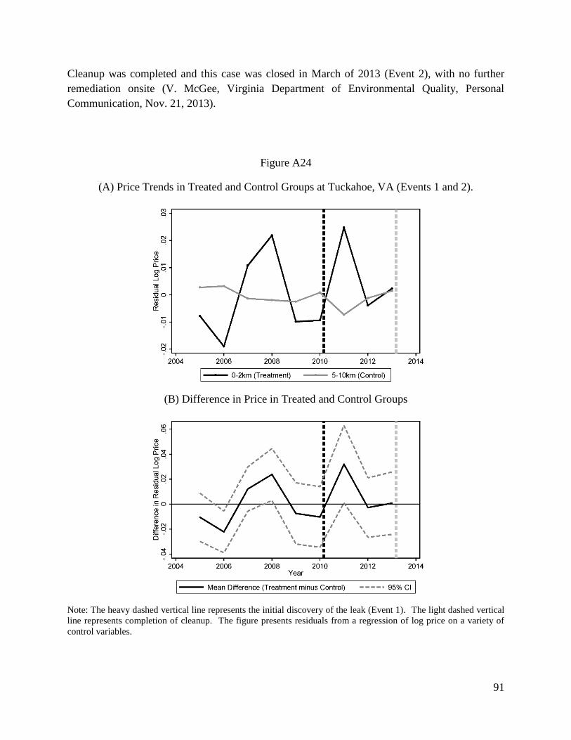
91

Cleanup was completed and this case was closed in March of 2013 (Event 2), with no further

remediation onsite (V. McGee, Virginia Department of Environmental Quality, Personal

Communication, Nov. 21, 2013).

Figure A24

(A) Price Trends in Treated and Control Groups at Tuckahoe, VA (Events 1 and 2).



line represents completion of cleanup. The figure presents residuals from a regression of log price on a variety of

control variables.

92

17. Pearl Street Gulf, Essex Junction, VT

In May of 2011, business owners at a shopping plaza in Essex Junction, Vermont smelled a strong

odor of gasoline coming from the parking lot and ultimately rising from a storm drain system. The

vapors were evaluated and deemed by local and state officials to be at combustible levels (Event

1). The shopping plaza was placed under evacuation orders and more than 15 businesses were

evacuated for a day while the vapors were vented and concentrations reduced (Reading 2011,

Association of State and Territorial Solid Waste Management Office 2014).

Inventory records at an adjacent gas station were reviewed and between 1,600 to 2,600 gallons of

gasoline were unaccounted for (Baird 2011). The release had occurred over a three-month period.

Inspections led to the discovery of a leaking submersible pump. For three weeks following

discovery of the release, the storm drains at the shopping center were vented with fans and treated

with a carbon filtration system. Over that period and despite removal/treatment of gasoline-

contaminated liquids, vapors in the system occasionally increased to explosive levels (Association

of State and Territorial Solid Waste Management Office 2014).

In mid-June, 2011, the gas station was ordered to remove all USTs to allow for an emergency

cleanup operation. In addition, soil removal was initiated and continued for a month. Following

tank and soil removal and site reconstruction, monitoring and recovery wells were installed. As of

April 2012, two monitoring points still contained petroleum volatile organic compounds in excess

of state groundwater enforcement standards (Association of State and Territorial Solid Waste

Management Office 2012a).

The Village of Essex Junction is located in the heart of Chittenden

County, Vermont, near the western border of Vermont and the shore of

Lake Champlain. It is 6 miles east of Burlington.






93

Figure A25

(A) Price Trends in Treated and Control Groups at Pearl Street Gulf, Essex Junct., VT (Event 1).


Note: The heavy dashed vertical line represents the initial discovery of the leak (Event 1). The figure presents


94

Works Cited in Appendix A

Adams, Noah. 2000. “Profile: Santa Monica’s Lawsuit Against Oil Companies for the

Contamination of Its Water Supply with MTBE.” All Things Considered, National Public

Radio. August 11.

Allen, Jim and Thomas Boving. 2006. “MTBE Drinking Water Contamination in Pascoag, RI: A

Tracer Test for Investigating the Fate and Transport of Contaminants in a Fractured Rock

Aquifer.” Final Report Submitted to Rhode Island Water Resources Center. Kingston.

June 05.

Allison, Jocelyn (2008) “ExxonMobil MTBE Gas Leak Suit To Go On” Law360. September 24.

Andreassi, G. (2001) Palm City neighbors praise start of cleanup. Stuart News. March 23.

Retrieved from http://infoweb.newsbank.com/iw-

search/we/InfoWeb?p_product=AWNB&p_theme=aggregated5&p_action=doc&p_docid

=0EB4C96CB30D1E3D&p_docnum=12&p_queryname=5 on 1/8/2015.

Andrews, P. (May 26, 2011). Wells contaminated in DeLeon, too. Gasoline-tainted water moves

towards DeLeon Springs West Volusia. The Beacon. Retrieved from

http://infoweb.newsbank.com/iw-


=1377EBF128755878&p_docnum=1&p_queryname=2 on 1/7/2015.

Andrews, P. (Jan 23, 2012). DeLeon may create EPA Brownfield- Designation could bring

revitalization $$. The Beacon. Retrieved from http://infoweb.newsbank.com/iw-


=13C787E12863D418&p_docnum=4&p_queryname=5 on 1/7/2015.

Association of State and Territorial Solid Waste Management Office (ASTSWMO). 2014.

Virginia Department of Environmental Quality. “Compendium of Emergency Response

Actions at Underground Storage Tank Sites: Version 2.” Final Report July 2014.

ASTSWMO LUST Task Force. Washington, D.C. October. Retrieved Jun 19, 2015 from

http://www.astswmo.org/Files/Policies_and_Publications/Tanks/2014.07_LUST%20ER

%20Compendium_v2.Final.pdf

Baird, Joel Banner. 2011. “Essex Junction gas leak claims contested.” Burlington Free Press.

Jun 22.

http://infoweb.newsbank.com/iw-search/we/InfoWeb?p_product=AWNB&p_theme=aggregated5&p_action=doc&p_docid=0EB4C96CB30D1E3D&p_docnum=12&p_queryname=5



http://infoweb.newsbank.com/iw-search/we/InfoWeb?p_product=AWNB&p_theme=aggregated5&p_action=doc&p_docid=1377EBF128755878&p_docnum=1&p_queryname=2



http://infoweb.newsbank.com/iw-search/we/InfoWeb?p_product=AWNB&p_theme=aggregated5&p_action=doc&p_docid=13C787E12863D418&p_docnum=4&p_queryname=5



95

Bellmore Public Meeting Slideshow. 2003. Received on Nov 19, 2013 by Robin Jenkins via

email from K. Gomez, New York State Department of Environmental Conservation.

September 25.

Colorado Department of Labor and Employment, (no date) Division of Oil and Public Safety

(OPS). Site Summary, Former Circle K Store, #1609; OPS Event ID 8882.

Cornelius, Coleman.2002. “Town’s Gas Leak Rated One of Worst in State.” The Denver Post.

April 9.

Crofton, Gregory. 2004. “Santa Monica fighting legal bills for MTBE lawsuit.” Tahoe Daily

Tribune. June 3. Accessed at

http://www.tahoedailytribune.com/article/20040604/NEWS/106040020

EnviroTrac Annual Update Report. 2011. Hess Station #32314, Bellmore, New York.

EnviroTrac Environmental Services. May 19.

Fan, Andrew. 2013. Telephone communication between Andrew Fan of US EPA Region 3 and

Robin Jenkins on July 24, 2013. (For notes, see final Chillum Fact Sheet on share drive.)

East Setauket. 2005. Final Remediation Status Report for the East Setauket Terminal

Remediation Project, NYSDEC Spill Case No. 87-6573. October 14.

ExxonMobil Oil Corporation. 2010. Quarterly Monitoring and System Report, Former Mobil

Service Station No. 10518. November 11. Attached to letter to Mr. Chris Engelhardt,

New York State Department of Environmental Conservation, Region 1.

Fisher, Dave. 2011. “No Causal Link?: MTBE’s Long Legacy in Pascoag.” ecoRI News.

September 07. Accessed Feb 4, 2015 at http://www.ecori.org/pollution-

contamination/2011/9/7/no-causal-link-mtbes-long-legacy-in-pascoag.html

Fitzgerald, Joseph. 2012. “Exxon Mobil to pay $7M to Pascoag water users.” The Call. June 9.

Accessed online through NewsBank Access World News on Feb 4, 2015.

Florida Springs Task Force. 2000. Florida’s Springs: Strategies for Protection & Restoration.

November. Accessed Jan 7, 2015 at

http://www.dep.state.fl.us/springs/reports/files/SpringsTaskForceReport.pdf

Gaines, Danielle E. 2014. “Settlement reached in Monrovia groundwater contamination lawsuit.”

June 4. Accessed online at

http://www.tahoedailytribune.com/article/20040604/NEWS/106040020

http://www.ecori.org/pollution-contamination/2011/9/7/no-causal-link-mtbes-long-legacy-in-pascoag.html

http://www.ecori.org/pollution-contamination/2011/9/7/no-causal-link-mtbes-long-legacy-in-pascoag.html

http://www.dep.state.fl.us/springs/reports/files/SpringsTaskForceReport.pdf

96

http://www.fredericknewspost.com/news/crime_and_justice/courts/settlement-reached-

in-monrovia-groundwater-contamination-lawsuit/article_16c93354-5358-5aa4-a77f-

adc65cef7f54.html on Jan 15, 2015.

Groundwater & Environmental Services, Inc. 2012. “MTBE Trend Analysis and Spill Closure

Request.” November.

Hess Bellmore Project Update. 2004. “Environmental Fact Sheet” September. Contact names on

this fact sheet include Dawn Coughlin, Amerad Hess Corporation; Karen Gomez, New

York State DEC; Robert Weitzman, Nassau County DOH.

Hirsch, Arthur. 2013. "High court won't reconsider most of ExxonMobil ruling". Baltimore Sun.

June 25. Accessed at http://www.baltimoresun.com/news/maryland/baltimore-

county/north-county/bs-md-co-exxon-decision-20130625-story.html#ixzz2pGxqSMEg

on Jan 13, 2015.

Holahan, Catherine. 2003. “Property purchases aid cleanup of pollution – Shell Oil affiliate

buying homes near gas leak site.” The Record (Hackensack, NJ), April 27.

Holahan, Catherine. 2004. “Shell Oil hid spill, lawsuit alleges – 10 homeowners in Montvale fear

impact on health.” The Record (Hackensack, NJ), January 9.

Jenks, Andy. 2010. “11,000+ gallons of gas spill into ground, stream.” NBC12 On Your Side.

March 22.

Kelly, Sean. 2002. “Gasoline Leak Forces La Salle Evacuations.” The Denver Post. March 27.

Leckie, Kate. 2010. “Damages rise to $3.75b in suit over water contamination.”

FrederickNewsPost.com. April 27.

Linder, Steve (2006). “Investigation and Remediation of Oxygenated Gasoline Releases

Containing Methyl tert-Butyl Ether (MTBE) Affecting Groundwater Supplies in

California, USA including the City of Santa Monica” PowerPoint presentation

(unpublished), received December 4, 2012.

Maryland Department of Environment. 2006. Fact Sheet: Upper Crossroads, Fallston, Maryland.

April 18. Accessed at http://www.weitzlux.com/mtbe/factsheet_403345.html on Jan. 12,

2015.

Maryland Department of Environment. 2008. Cleanup Actions and Environmental Investigation

at the Jacksonville Exxon. September 11. Accessed at

http://www.fredericknewspost.com/news/crime_and_justice/courts/settlement-reached-in-monrovia-groundwater-contamination-lawsuit/article_16c93354-5358-5aa4-a77f-adc65cef7f54.html%20on%20Jan%2015



http://www.baltimoresun.com/news/maryland/baltimore-county/north-county/bs-md-co-exxon-decision-20130625,0,2425441.story#ixzz2pGxqSMEg

http://en.wikipedia.org/wiki/Baltimore_Sun

http://www.baltimoresun.com/news/maryland/baltimore-county/north-county/bs-md-co-exxon-decision-20130625-story.html#ixzz2pGxqSMEg

http://www.baltimoresun.com/news/maryland/baltimore-county/north-county/bs-md-co-exxon-decision-20130625-story.html#ixzz2pGxqSMEg

http://www.weitzlux.com/mtbe/factsheet_403345.html

97

http://www.mde.state.md.us/programs/Land/OilControl/RemediationSites/Documents/w

ww.mde.state.md.us/assets/document/OilControl/BaltoCo-

JacksonExxonMobil_Fact_Sheet_Sept11_08.pdf on Jan. 13, 2015.

Maryland Department of Environment. 2010. Fact Sheet: MDE Case 94-12-51-HA. October 1.

Accessed at

http://www.mde.state.md.us/programs/Land/OilControl/RemediationSites/Documents/Ha

rford%20Former%20Upper%20Crossroads.pdf on Jan 13, 2015.

Maryland Department of Environment. 2010b. Green Valley Citgo Environmental Investigation

and Monitoring Well Impact. Fact Sheet. April 12. Accessed at

http://www.mde.state.md.us/programs/land/oilcontrol/remediationsites/pages/programs/la

ndprograms/oil_control/remediationsites/index.aspx on Jan. 15, 2015.

Maryland Department of Environment. 2014. Groundwater Monitoring and Remedial Status

Report Inactive Exxon Facility #28077. November 14. Accessed at



Maryland Department of Environment. 2014b. Private Supply Well Charts. November 24.

Accessed at



Maryland Department of Environment. 2014c. Third Quarter 2014 Monitoring Report.:

Monrovia BP/Former Green Valley Citgo. November 15. Accessed at



Maryland Department of Environment. 2015. Approval for Monitoring Well Abandonment: Case

no. 2005-0834-FR, Green Valley Citgo. October 27. Accessed at

http://mde.maryland.gov/programs/Land/OilControl/RemediationSites/Documents/FR%2

0Co%20-

%20GV%20Citgo%20Approval%20for%20MW%20Abandonment%2010.27.15%205%

20pgs.pdf on Jan. 29, 2016.

Metzger, Harrison. 2003. “State to discuss wells at meeting: Officials focus tests on area

southwest of crossroads.” October 1. Accessed at

http://www.blueridgenow.com/article/20031001/NEWS/310010333?p=2&tc=pg on Jan

15, 2015.

http://www.mde.state.md.us/programs/Land/OilControl/RemediationSites/Documents/www.mde.state.md.us/assets/document/OilControl/BaltoCo-JacksonExxonMobil_Fact_Sheet_Sept11_08.pdf



http://www.mde.state.md.us/programs/Land/OilControl/RemediationSites/Documents/Harford%20Former%20Upper%20Crossroads.pdf

http://www.mde.state.md.us/programs/Land/OilControl/RemediationSites/Documents/Harford%20Former%20Upper%20Crossroads.pdf

http://www.mde.state.md.us/programs/land/oilcontrol/remediationsites/pages/programs/landprograms/oil_control/remediationsites/index.aspx








http://mde.maryland.gov/programs/Land/OilControl/RemediationSites/Documents/FR%20Co%20-%20GV%20Citgo%20Approval%20for%20MW%20Abandonment%2010.27.15%205%20pgs.pdf




http://www.blueridgenow.com/article/20031001/NEWS/310010333?p=2&tc=pg

98

Metzger, Harrison. 2005. “Tainted water problem is fixed.” BlueRidgeNow.com Times-News.

Dec. 7. Accessed at

http://www.blueridgenow.com/apps/pbcs.dll/article?p=2&tc=pg&AID=/20051207/NEW

S/512070342/1042 on Jan. 15, 2015.

Mitchell, Josh. 2005. “Gas station in Fallston tied to leaks of MTBE and fouled wells is closed,”

Baltimore Sun. April 28. Accessed at http://www.baltimoresun.com/bal-

md.ha.mtbe28apr28-story.html on Jan. 12, 2015.

Montvale, NJ. (n.d.). In Wikipedia. Retrieved Jan 20, 2015, from

http://en.wikipedia.org/wiki/Montvale,_New_Jersey

Neibauer, Michael. 2012. “Chevron to Pay D.C. $500K for Gas Spill,” Washington Business

Journal. January 27.

New Jersey Department of Environmental Protection. 2012. Site Remediation Program Active

Sites With Confirmed Contamination, April. Retrieved Jan 20, 2015 from

http://www.nj.gov/dep/srp/kcsnj/kcsnj_active.pdf.

New York State Comptroller. 2007. News from the Office of the New York State Comptroller,

Thomas P. DiNapoli. August 29.

New York State Department of Environmental Conservation. 2006. Fact Sheet: Northville

Terminal, Terminal Road. November. <Share drive>

New York State Department of Environmental Conservation. 2007. Fact Sheet: MTBE

Contamination, Birch Street Plant. February. <See final fact sheet on share drive.>

North Carolina Department of Environment and Natural Resources. 2004. Annual Report to the

North Carolina General Assembly Environmental Review commission: The Status of

Leaking Petroleum Underground Storage Tanks, the State Cleanup Funds, and the

Groundwater Protection Loan Fund. September 1. <Stored on share drive>

Oculus. 2013. Florida State database; Facility ID #s: 43/8511465; 43/8520079 and 43/8520084.

Oculus. 2015. Florida state database; Facility ID #: 48-8513391 at

http://depedms.dep.state.fl.us/Oculus/servlet/login

http://www.baltimoresun.com/bal-md.ha.mtbe28apr28-story.html

http://www.baltimoresun.com/bal-md.ha.mtbe28apr28-story.html

http://en.wikipedia.org/wiki/Montvale,_New_Jersey

http://www.nj.gov/dep/srp/kcsnj/kcsnj_active.pdf

http://depedms.dep.state.fl.us/Oculus/servlet/login

99

Pascoag, Rhode Island. (n.d.). In Wikipedia. Retrieved Feb 3, 2015 from

http://en.wikipedia.org/wiki/Pascoag,_Rhode_Island

Pulver, Dinah Voyles. 2014. “Cleanup of decades-old DeLeon Springs gasoline leak has started

again,” Daytona Beach News-Journal. April 30. Retrieved Jan 7, 2015 from



=14D83DAB6BCC6318&p_docnum=1&p_queryname=1

Reading, Jennifer. 2011. “Essex Jct Gas Leak may be Larger than Thought.” WCAX News. June

20.

Rocky Mountain News. 2002. News Staff and wire reports. “Cleanup of Gas Spill Begins.” April

10.

Roe, R. (2012). Establishment of an alternative water supply in the Bithlo community of Orange

County, FL 2011-2012. National Environmental Public Health Leadership Institute.

Santa Monica News Release. 2011. “Santa Monica Achieves Landmark Sustainability Milestone

with Opening of Water Treatment Plant.” Targeted News Service (USA). February 24.

Santana, Arthur. 2004. “Waiting for a verdict on an underground threat: Residents seek answers

on gas, cleaning chemicals in soil, water of Riggs Park.” Washington Post. Feb. 8.

Schmitt, Eric. 1990. “Gas Spill Cleanup Turns L.I. Backyards Into Field Labs,” The New York

Times. May 14.

Schweisberg, Kim. 2005. “Beyond Inspection Targeting: Lessons From Pascoag, RI,”

UST/LUST National Conference, Seattle, WA. EPA New England UST/LUST Team.

Smith, Jennifer. 2007. “Troubled gas station linked to MTBE leak.” Newsday. February 5.

Sobel, Elizabeth W. 2006. “Northville gas spill cleanup declared complete,”

Northshoreoflongisland.com. November 17.

Sorentrue, J. 2003. Leaks fuel worries in Old Palm City. The Palm Beach Post. December 14.

Retrieved Jan 8, 2015 from http://infoweb.newsbank.com/iw-


=0FF75ACE2551F239&p_docnum=6&p_queryname=4

http://en.wikipedia.org/wiki/Pascoag,_Rhode_Island

http://infoweb.newsbank.com/iw-search/we/InfoWeb?p_product=AWNB&p_theme=aggregated5&p_action=doc&p_docid=14D83DAB6BCC6318&p_docnum=1&p_queryname=1



http://infoweb.newsbank.com/iw-search/we/InfoWeb?p_product=AWNB&p_theme=aggregated5&p_action=doc&p_docid=0FF75ACE2551F239&p_docnum=6&p_queryname=4



100

Springston, Rex. 2010. “Cleanup of spilled gas continues at Henrico Uppy’s.” Richmond Times

Dispatch. March 18.

Three Village Times. 2006. “WH, FS Residents Advised Not to Use Tap Water.” Jun 30.

Tonyan, R. 1987. Gas tanks seal may be the cause of leak investigators pinpoint possible

problem. The Orlando Sentinel. May 28. Retrieved on Jan 7, 2015 from



=0EB4EB92663F8180&p_docnum=3&p_queryname=4

Tyko, K. 2006. New station coming to Palm City. Stuart News. Dec 27. Retrieved on Jan 8,

2015 from http://infoweb.newsbank.com/iw-


=11651C1B8C5689F0&p_docnum=11&p_queryname=5

Universal Solutions, Inc. 2005. Remedial Action Plan (RAP) Deleon Springs Florida. December.

US Census Bureau. State and County Quickfacts for socioeconomic descriptive statistics for the

case profile boxes. http://quickfacts.census.gov/qfd/index.html.

US City-Data.com (for population, income, and race statistics for Monrovia, MD):

http://www.city-data.com/city/Monrovia-Maryland.html

USA.com. (for socioeconomic descriptive statistics for Lasalle, CO) Uses U.S. Census American

Community Survey data for 2008-2012. World Media Group. Basking Ridge, NJ.

http://www.usa.com/la-salle-co.htm

USA.com (for population density in Monrovia, MD). World Media Group, Basking Ridge, NJ.

http://www.usa.com/monrovia-md-population-and-races.htm

US Department of Justice. 2005. “Oil Companies Pay EPA to Settle Santa Monica MTBE

Cleanup Costs” February 16. Retrieved Oct 20, 2014 from

http://www.justice.gov/opa/pr/2005/February/05_enrd_067.htm

US Environmental Protection Agency Region 3. 2008. News Releases from Region 3: EPA

Issues Final Decision for Chevron Cleanup for a Gasoline Release on the D.C. -

Maryland Border. April 16. Retrieved Jan 9, 2015 from

http://yosemite.epa.gov/opa/admpress.nsf/90829d899627a1d98525735900400c2b/34abea

f210bf7ed48525742d006cc829!OpenDocument

http://infoweb.newsbank.com/iw-search/we/InfoWeb?p_product=AWNB&p_theme=aggregated5&p_action=doc&p_docid=0EB4EB92663F8180&p_docnum=3&p_queryname=4



http://infoweb.newsbank.com/iw-search/we/InfoWeb?p_product=AWNB&p_theme=aggregated5&p_action=doc&p_docid=11651C1B8C5689F0&p_docnum=11&p_queryname=5



http://www.city-data.com/city/Monrovia-Maryland.html

http://www.usa.com/la-salle-co.htm

http://www.usa.com/monrovia-md-population-and-races.htm

http://www.justice.gov/opa/pr/2005/February/05_enrd_067.htm

http://yosemite.epa.gov/opa/admpress.nsf/90829d899627a1d98525735900400c2b/34abeaf210bf7ed48525742d006cc829!OpenDocument

http://yosemite.epa.gov/opa/admpress.nsf/90829d899627a1d98525735900400c2b/34abeaf210bf7ed48525742d006cc829!OpenDocument

101

US Environmental Protection Agency Region 3. 2009. Chillum Site – Gasoline Fact Sheet.

September.

http://www3.epa.gov/reg3wcmd/ca/pdf/Chevron_ChilllumMD_FinalRemedy.pdf

US Environmental Protection Agency Region 3. 2015. Mid Atlantic RCRA Land Cleanup.

Chevron U.S.A. – Chillum MD. Retrieved Jan 9, 2015 from

http://www.epa.gov/reg3wcmd/chev7003.htm

Vargas, Theresa (2004) “Seeking Answers on Gas Leak” Tank and Petroleum Use Mishaps.

April.

Water Supply Analysis-Bithlo Rural Settlement. Summary Report, October 2011.

WFTV.com. (November 22, 2011). Bithlo residents have differing views on contaminated well

lines. Retrieved from http://www.wftv.com/news/news/local/bithlo-residents-have-

differing-views-contaminated/nFkQR/ on 8/20/2013.

Wheeler, Timothy B. 2004. State considers new MTBE rules. Baltimore Sun. July 21. Retrieved

Jan 12, 2015 from http://www.chicagotribune.com/business/bal-md.mtbe21jul21-

story.html

White, Michael. 2006. “Water Tainted by Gas. Warning not to drink in West Hempstead.” New

York Daily News. June 28.

Zabel, Jeffrey E. and Dennis Guignet. 2012. “A Hedonic Analysis of the Impact of LUST Sites

on House Prices,” Resource and Energy Economics, 34(4), 549-564.

http://www.epa.gov/reg3wcmd/chev7003.htm

http://www.wftv.com/news/news/local/bithlo-residents-have-differing-views-contaminated/nFkQR/

http://www.wftv.com/news/news/local/bithlo-residents-have-differing-views-contaminated/nFkQR/

http://www.chicagotribune.com/business/bal-md.mtbe21jul21-story.html

http://www.chicagotribune.com/business/bal-md.mtbe21jul21-story.html

102

Appendix B: Meta-data Quasi-Experimental Diagnostics

Even though a quasi-experimental interpretation may not be valid for the primary hedonic

framework at some high-profile sites, perhaps such an interpretation is reasonable when

considering all sites as a whole. We posit that potentially confounding factors are reduced by

examining multiple sites in our internal meta-analysis. In a valid quasi-experiment, diagnostic

comparisons of the treated and control groups would suggest similar time trends prior to the

treatment event, and then, if there is a measurable treatment effect, demonstrate a divergence in

these trends after treatment. Analogous to the price trend differential graphs presented in Appendix

A and discussed in section V.B, a graph of the corresponding meta-data (i.e., estimates from the

primary hedonic regressions) is developed here.

For each of the 12 high-profile sites where we observed the discovery of a release, the

below hedonic regression is estimated (equation B1). Similar to the hedonic analyses the

corresponding samples are constrained to only sales within 5 years before or after the discovery of

the release. In contrast, here the regression for each of the sites is estimated using only houses

within 0-2 km (the treated group) or within 5-10 km (the control group) of the high-profile site.

The treatment event (or release discovery in this case) occurred at a different date for each

site, ranging from the Deleon Springs release in June, 1985 in Florida, to the Pearl Street Gulf

release in May, 2011 in Vermont. Treatment assignment is fairly well dispersed over space and

time, and so even if primary estimates from one specific location suffered from an omitted variable

bias, one could hypothesize that the probability of the same confounding influences systematically

existing at all treatment locations and times may be relatively low.

For each high-profile site s, time was normalized with respect to the release date, and

transactions were grouped into one year bins relative to the date of the release. Following this

103

normalization, sT is a dummy variable denoting that the transaction took place in year τ relative to

the date the release was discovered at site s. An interaction term between the time dummy

variables and a dummy variable equal to one for homes within 0-2km of the high-profile site

0 2km

isD is also included. The primary hedonic regressions that are estimated for each of the 12

high-profile sites in this exercise is:

0 2ln km

ij s ij s s s is s j ij sp x T T D v (B1)

The vector xijτ contains all structural, parcel, neighborhood, and other control variables that are not

of direct interest, vj is a neighborhood fixed effect (at the census tract level), and εijts is a normally

distributed and assumed mean zero error term. The coefficients to be estimated are β, s , s ,

and jv . The coefficient of interest is s , which reflects the price differential between the time

trends for the treated and control groups. Taking the estimates of s for each of the high-profile

sites s, we estimated the percent difference in prices between the treated and control groups in year

τ as:

% ( 1) 100s

sp e

(B2)

These estimates compose the meta-data used to graph the price trend differential at the meta-

analysis level. Notice that the release discovery or “treatment” date is not specified. These

estimates reflect the general trends over time without imposing any structure with respect to the

treatment date.

Next the meta-data are used to estimate the following random effect size (RES) meta-

regression:

104

0 1ˆ% s s sp T e (B3)

where 0 is a constant term to be estimated, and 1 is a coefficient vector that reflects the average

price differential in each year τ between the treated and control groups. Note that 5 years before

the release is discovered (τ = -5) is the omitted category. The estimated price trend differential is

depicted in the below graph (which corresponds to Figure 5 in the main text). Again, we emphasize

that no structure was imposed relative to the release discovery date. This trend merely reflects the

difference between how the treated group prices changed over time relative to the control group.

Figure B1. Meta-analytic Price Trend Differential Between Treated and Control Groups.

(Same as Figure 5 in main text.)

Note: Treated group houses within 0-2 km from a high-profile site, and control group as houses from 5-10 km.

The confidence intervals are fairly wide given the small number of transactions in the

treated group when divided up into annual bins, but the point estimates reveal an interesting story.

The near zero, and even slightly positive, difference in the left portion of the graph suggests that

there was little difference in price between the treated and control groups before the release was

discovered, on average. In contrast, the negative point estimates in the right portion of the graph

-40

-30

-20

-10

0

10

20

30

40

-5 -4 -3 -2 -1 1 2 3 4 5

% Δ

Pri

ce

Time (years)Release Discovered

105

suggest that prices among homes within 0-2km of the high-profile site (the treated group) are

slightly lower relative to homes located at 5-10km away from the site (the control group) after the

discovery of the release (i.e., post treatment). Again, these differences are not statistically

significant, which is not surprising given the small number of transactions each year in the treated

group (and hence wide confidence intervals in the meta-data), but the story is consistent with the

notion that the meta-analysis provides a valid quasi-experiment as a whole, even when such an

interpretation may not necessarily be appropriate among some study locations in the primary

hedonic analysis.

106

Appendix C: Full Hedonic Regression Results

Table C.1. Full Regression Results for Models 1 through 3: Dep Var. = ln(price).

Model 1 Model 2 Model 3

Charnock Well Fields, CA LaSalle, CO LaSalle, CO

VARIABLESa Period 1 Period 1 Period 2

Age of House -0.001987* -0.000808 -0.004815***

(0.001) (0.002) (0.002)

Age Missing -0.297820*** 0.793372*** 0.002209

(0.101) (0.136) (0.240)

Age^2 0.000023** -0.000002 0.000014

(0.000) (0.000) (0.000)

Townhome -0.247056*** 0.008797 -0.071479

(0.061) (0.046) (0.043)

Total # Bathrooms 0.023993*** 0.010875 0.093184***

(0.006) (0.032) (0.010)

Bathrooms Missing -0.308792 -0.044891 0.737436***

(0.294) (0.094) (0.129)

ln(interior square footage) 0.501674*** 0.168114*** 0.164274***

(0.026) (0.048) (0.041)

Square Footage Missing 4.150611*** 1.021012*** 0.945592***

(0.440) (0.264) (0.279)

ln(lot acreage) 0.062002* 0.009445 0.202088***

(0.036) (0.035) (0.033)

Acreage Missing -0.060676 -0.208763***

(0.075) (0.073)

Air Conditioner -0.058733* 0.014002

(0.030) (0.026)

Air Conditioner Missing 0.122182

(0.306)

Basement 0.119095** 0.143494***

(0.053) (0.025)

Basement Missing - -

Porch -0.105323 0.009577

(0.111) (0.067)

Porch Missing

Pool 0.095846***

(0.012)

Pool Missing

Distance to nearest urban cluster (km) -80.269636 -23.104865***

(58.697) (7.744)

Distance to nearest urban cluster (meters) 0.037913**

(0.016)

Distance to nearest major road (km) 0.043634** -0.013159 -0.054742***

(0.019) (0.064) (0.015)

107

In a 100 yr floodplain -0.004250

(0.030)

Public Water Service Area (PWS)

PWS Area Missing

Waterfront

# of gas stations w/in 200 meters -0.040894*** 0.033800 -0.036220**

(0.008) (0.029) (0.016)

# of gas stations w/in 200-500 meters -0.012290*** -0.016705 -0.016444

(0.004) (0.023) (0.010)

1 km from High-profile (HP) Site 0.057715 -0.176997 0.038950

(0.073) (0.302) (0.080)

1-2 km from HP Site 0.038704 -0.001508 -0.414066

(0.063) (0.310) (0.405)

2-3 km from HP Site 0.031306 0.214849 -0.081789

(0.046) (0.261) (0.120)

3-4 km from HP Site 0.018598 0.145933 -0.039592

(0.040) (0.234) (0.126)

4-5 km from HP Site 0.002229 -0.087074 -0.042041

(0.032) (0.067) (0.067)

Event 1 × 1 km from HP Site 0.073830*** -0.317473***

(0.022) (0.065)

Event 1 × 1-2 km from HP Site 0.085157*** -0.407769

(0.019) (0.265)

Event 1 × 2-3 km from HP Site 0.082835*** -0.714429***

(0.015) (0.122)

Event 1 × 3-4 km from HP Site 0.092824*** -0.616086***

(0.023) (0.090)

Event 1 × 4-5 km from HP Site 0.053280** -0.263739**

(0.024) (0.112)

Event 2 × 1 km from HP Site 0.075590

(0.058)

Event 2 × 1-2 km from HP Site 0.589011***

(0.103)

Event 2 × 2-3 km from HP Site 0.019437

(0.074)

Event 2 × 3-4 km from HP Site -0.026653

(0.052)

Event 2 × 4-5 km from HP Site -0.121682***

(0.036)

Quarterly Dummies Yes Yes Yes

Annual Dummies 2006-2013 1997-2007 2004-2013

Tract FE Yes Yes Yes

# of FE 236 24 23

Observations 27,597 31,118 16,334

Adj. R-squared 0.450 0.188 0.228

*** p<0.01, ** p<0.05, * p<0.1. Robust standard errors in parentheses, clustered by Census Tract.

a. All variables are binary indicators unless otherwise noted.

108



Bithlo, FL Bithlo, FL Bithlo, FL


Age of House 0.016686 0.007559 0.010254*

(0.010) (0.015) (0.005)

Age Missing -1.205105*** -0.705305*** -0.046024

(0.049) (0.071) (0.088)

Age^2 -0.000466* -0.000157 -0.000235*

(0.000) (0.000) (0.000)

Townhome -0.340735*** -0.204546***

(0.054) (0.016)

Total # Bathrooms 0.093201** 0.077614*** 0.048922**

(0.031) (0.016) (0.016)

Bathrooms Missing 2.406279* 0.097313 -0.002705

(0.966) (0.146) (0.115)

ln(interior square footage) 0.309667* 0.532039*** 0.726676***

(0.130) (0.045) (0.047)

Square Footage Missing 4.280033*** 5.125086***

(0.352) (0.364)

ln(lot acreage) 0.239112*** 0.358419*** 0.435787***

(0.047) (0.063) (0.062)

Acreage Missing 0.093049 0.364035*** 0.202612***

(0.124) (0.063) (0.042)

Air Conditioner

Air Conditioner Missing

Basement

Basement Missing

Porch

Porch Missing

Pool

Pool Missing

Distance to nearest urban cluster (km)

Distance to nearest urban cluster (meters) 0.027231 -0.032676 -0.071511**

(0.019) (0.027) (0.028)

Distance to nearest major road (km) -0.001789 -0.068091** -0.056591

109

(0.022) (0.019) (0.031)

In a 100 yr floodplain 0.226134 -0.004641 -0.107942***

(0.184) (0.132) (0.008)


PWS Area Missing

Waterfront

# of gas stations w/in 200 meters -0.271480 -0.192739 -0.181561**

(0.232) (0.134) (0.054)

# of gas stations w/in 200-500 meters 0.095334 -0.061034 0.019245

(0.048) (0.078) (0.037)

1 km from High-profile (HP) Site -0.506267* -0.952495*** -0.971445***

(0.200) (0.116) (0.206)

1-2 km from HP Site -0.187943 -0.711109*** -0.433727***

(0.231) (0.145) (0.109)

2-3 km from HP Site -0.311183 -0.458026** -0.255530**

(0.164) (0.177) (0.074)

3-4 km from HP Site -0.245720* -0.294375** -0.113414***

(0.106) (0.105) (0.022)

4-5 km from HP Site -0.274444*** -0.350408*** 0.032743

(0.067) (0.059) (0.029)


(0.111)


(0.291)


(0.163)

Event 1 × 3-4 km from HP Site 0.241360**

(0.085)

Event 1 × 4-5 km from HP Site 0.306504*

(0.121)

Event 2 × 1 km from HP Site -0.020541

(0.086)


(0.165)


(0.144)


(0.089)

Event 2 × 4-5 km from HP Site 0.233470***

(0.037)

Event 3 × 1 km from HP Site 0.304411**

(0.106)


(0.152)


110

(0.074)


(0.037)


(0.073)


Annual Dummies 1983-1993 1998-2008 2006-2013


# of FE 6 7 7

Observations 5,383 33,290 8,739

Adj. R-squared 0.487 0.419 0.613



111


Model 7 Model 8 Model 9 Model 10 Model 11

DeLeon Springs, FL DeLeon Springs, FL Palm City Cluster, FL Palm City Cluster, FL Palm City Cluster, FL

VARIABLESa Period 1 Period 2 Period 1 Period 2 Period 3

Age of House 0.028430*** 0.026956** 0.011899* -0.005808 -0.013387***

(0.005) (0.009) (0.006) (0.005) (0.004)

Age Missing -1.277399*** -1.151720*** 0.281439 -0.344564 -1.027592***

(0.054) (0.070) (0.191) (0.295) (0.123)

Age^2 -0.000473*** -0.000462** -0.000168 0.000055 0.000146**

(0.000) (0.000) (0.000) (0.000) (0.000)

Townhome 0.122546 0.106399 0.078379 -0.062937 -0.134509

(0.064) (0.073) (0.079) (0.119) (0.129)

Total # Bathrooms 0.087103*** 0.090316*** 0.018281 -0.039236 0.093655***

(0.012) (0.018) (0.037) (0.032) (0.017)

Bathrooms Missing 0.253097 -0.374102 5.569753*** 0.217952

(0.164) (0.442) (0.780) (0.198)

ln(interior square footage) 0.476240*** 0.465210*** 0.382368** 0.838308*** 0.543720***

(0.080) (0.064) (0.147) (0.095) (0.084)

Square Footage Missing 2.786391** 4.396570***

(0.979) (0.640)

ln(lot acreage) 0.245077*** 0.165589*** -0.133528* 0.020753 0.267605***

(0.035) (0.029) (0.071) (0.080) (0.038)

Acreage Missing -0.187407*** -0.146123*** 0.180392 -0.164748 -1.036464***

(0.007) (0.016) (0.207) (0.185) (0.175)

Air Conditioner 0.317082*** 0.150697** 0.105682

(0.089) (0.059) (0.083)


Basement 0.176798 0.269278*** 0.263754***

(0.180) (0.089) (0.086)

Basement Missing

Porch -0.085456 0.102370 -0.086365

(0.127) (0.065) (0.063)

Porch Missing 0.231983* 0.941917*** 0.617553***

(0.118) (0.142) (0.108)

Pool 0.080762* 0.077714* 0.057525***

(0.042) (0.045) (0.019)

Pool Missing 0.158460*** 0.000942 0.056012

(0.052) (0.043) (0.073)

Distance to nearest urban

cluster (km)


cluster (meters) -0.011220 -0.062009* 0.088333** 0.081503** 0.082514***

(0.018) (0.025) (0.033) (0.029) (0.020)

112

Distance to nearest major road

(km) 0.056663** 0.101435*** 0.043717 0.068518* -0.038793

(0.022) (0.019) (0.036) (0.036) (0.050)

In a 100 yr floodplain -0.206211 0.011439

(0.153) (0.034)

Public Water Service Area

(PWS) -0.129561 0.072157 0.054175

(0.101) (0.119) (0.081)

PWS Area Missing

Waterfront 0.437413*** 0.328688*** 0.274326***

(0.146) (0.099) (0.065)

# of gas stations w/in 200

meters -0.069926** 0.107860 -0.441773*** -0.343321*** -0.234909***

(0.026) (0.059) (0.142) (0.088) (0.069)

# of gas stations w/in 200-500

meters -0.043818 -0.043684 -0.239672*** -0.238481*** -0.140905**

(0.033) (0.038) (0.072) (0.071) (0.056)

1 km from High-profile (HP)

Site -0.441199* -0.509615** -0.419117* -0.390382** -0.176771

(0.186) (0.174) (0.212) (0.180) (0.190)

1-2 km from HP Site -0.558737** -0.455084** 1.327383** -0.403363* -0.117578

(0.145) (0.163) (0.512) (0.201) (0.205)

2-3 km from HP Site -0.222622* -0.028712 0.517587** 0.218890 0.031449

(0.109) (0.070) (0.229) (0.171) (0.213)

3-4 km from HP Site -0.306166*** -0.131206* -0.173877 -0.034648 0.224554

(0.072) (0.065) (0.111) (0.178) (0.131)

4-5 km from HP Site -0.283046*** -0.079610 -0.149328* -0.139843 0.297247

(0.041) (0.067) (0.085) (0.148) (0.186)

Event 1 × 1 km from HP Site -0.146363*** -0.104296**

(0.015) (0.038)

Event 1 × 1-2 km from HP Site 0.059795 -1.527393***

(0.058) (0.493)


(0.008) (0.370)

Event 1 × 3-4 km from HP Site 0.148008** 0.404126***

(0.051) (0.092)

Event 1 × 4-5 km from HP Site 0.162425* -0.011401

(0.078) (0.044)

Event 2 × 1 km from HP Site 0.190792*** 0.059935

(0.016) (0.050)

Event 2 × 1-2 km from HP Site 0.062778 0.269882***

(0.039) (0.093)

Event 2 × 2-3 km from HP Site -0.214746* -0.277958

(0.090) (0.167)

Event 2 × 3-4 km from HP Site -0.117717 0.070055

(0.067) (0.079)

Event 2 × 4-5 km from HP Site -0.147853 0.047559

113

(0.166) (0.072)

Event 3 × 1 km from HP Site -0.129330***

(0.032)


(0.031)


(0.079)


(0.172)


(0.109)

Quarterly Dummies Yes Yes Yes Yes Yes

Annual Dummies 1980-1990 1985-1995 1983-1992 1991-2001 2003-2013

Tract FE Yes Yes Yes Yes Yes

# of FE 6 6 20 20 19

Observations 5,971 6,036 20,874 25,949 21,325

Adj. R-squared 0.530 0.493 0.199 0.205 0.444



114


Model 12 Model 13 Model 14 Model 15

Chillum, MD Upper Crossroads, MD Upper Crossroads, MD Jacksonville Exxon, MD

VARIABLESa Period 1 Period 1 Period 2 Period 1

Age of House -0.001413*** -0.005516*** -0.006827*** -0.006060***

(0.000) (0.001) (0.001) (0.001)

Age Missing -0.157002*** -0.330638*** -0.367114*** -0.268161***

(0.023) (0.094) (0.077) (0.085)

Age^2 0.000001*** 0.000024*** 0.000030*** 0.000032***

(0.000) (0.000) (0.000) (0.000)

Townhome -0.123296*** -0.125370*** -0.140335*** -0.099157**

(0.021) (0.014) (0.025) (0.041)

Total # Bathrooms 0.059051*** 0.052397*** 0.042863*** 0.053590***

(0.003) (0.016) (0.007) (0.013)

Bathrooms Missing -0.607287*** -0.312884***

(0.039) (0.048)

ln(interior square footage) 0.379572*** 0.408276*** 0.373079*** 0.459916***

(0.017) (0.014) (0.017) (0.039)

Square Footage Missing 3.110271*** 3.104216*** 2.792784*** 3.574613***

(0.135) (0.240) (0.201) (0.299)

ln(lot acreage) 0.099273*** 0.105700*** 0.105969*** 0.101457***

(0.011) (0.008) (0.007) (0.017)

Acreage Missing -0.153709 -0.597077***

(0.174) (0.025)

Air Conditioner 0.035742*** 0.042485*** 0.054651*** 0.101176***

(0.004) (0.010) (0.012) (0.014)


Basement 0.097404*** -0.017107 -0.001751 0.034029**

(0.006) (0.010) (0.006) (0.014)

Basement Missing

Porch 0.031050*** 0.030122** 0.066944***

(0.003) (0.012) (0.020)

Porch Missing 0.026174*** 0.010098 0.075816**

(0.006) (0.026) (0.031)

Pool 0.002493 0.051274*** 0.025214

(0.022) (0.010) (0.021)

Pool Missing


(km) -0.039932*** 0.007710* 0.005304 0.003391

(0.015) (0.004) (0.004) (0.010)


(meters)


(km) 0.036092*** -0.003278 0.000111 -0.010834

(0.012) (0.005) (0.004) (0.009)

115

In a 100 yr floodplain -0.053749*** -0.073564* -0.073041 0.161653***

(0.018) (0.035) (0.048) (0.056)

Public Water Service Area (PWS) 0.018733 0.016410 0.059376*

(0.030) (0.013) (0.030)

PWS Area Missing

Waterfront

# of gas stations w/in 200 meters -0.011997* -0.038397 -0.032628 -0.012895

(0.007) (0.030) (0.031) (0.021)


meters 0.004534 -0.010821 -0.003153 -0.017433

(0.003) (0.012) (0.005) (0.015)

1 km from High-profile (HP) Site -0.222753** 0.073876*** 0.051146** 0.119741*

(0.088) (0.019) (0.020) (0.067)

1-2 km from HP Site -0.149087*** 0.044091** 0.079999*** 0.033929

(0.054) (0.018) (0.019) (0.056)

2-3 km from HP Site -0.111270** 0.043164 0.052829** 0.039506

(0.049) (0.027) (0.021) (0.062)

3-4 km from HP Site -0.115186*** -0.038610 0.029998 0.093339

(0.029) (0.040) (0.021) (0.061)

4-5 km from HP Site -0.078156*** 0.022469* 0.053742** 0.058787

(0.016) (0.012) (0.018) (0.046)

Event 1 × 1 km from HP Site 0.005825 -0.043663*** -0.160673***

(0.014) (0.011) (0.014)

Event 1 × 1-2 km from HP Site 0.022525*** 0.029675*** -0.053097

(0.007) (0.008) (0.038)

Event 1 × 2-3 km from HP Site 0.036813* -0.008588 -0.070008***

(0.019) (0.009) (0.011)

Event 1 × 3-4 km from HP Site 0.040883*** 0.046789 -0.039360

(0.011) (0.035) (0.024)

Event 1 × 4-5 km from HP Site 0.050490*** 0.014264 -0.039204*

(0.010) (0.021) (0.022)


(0.014)

Event 2 × 1-2 km from HP Site -0.058739***

(0.015)

Event 2 × 2-3 km from HP Site -0.030197*

(0.014)


(0.015)


(0.030)

Quarterly Dummies Yes Yes Yes Yes

Annual Dummies 1996-2006 1996-2003 1999-2009 2001-2009

Tract FE Yes Yes Yes Yes

# of FE 122 10 10 28

Observations 65,574 4,245 7,176 8,154

Adj. R-squared 0.775 0.793 0.856 0.743



116


Model 16 Model 17 Model 18 Model 19


Hendersonville

Corner Pantry

, NC Montvale, NJ Montvale, NJ

VARIABLESa Period 1 Period 1 Period 1 Period 2

Age of House -0.003264*** -0.003527*** -0.005270*** -0.006294***

(0.000) (0.001) (0.001) (0.001)

Age Missing -0.317500** -1.430659*** -0.207967*** -0.260668***

(0.096) (0.101) (0.049) (0.045)

Age^2 0.000004*** 0.000014 0.000024*** 0.000029***

(0.000) (0.000) (0.000) (0.000)

Townhome -0.127665*** 0.045250

(0.020) (0.065)

Total # Bathrooms 0.049857*** 0.018640

(0.008) (0.012)

Bathrooms Missing -0.504805*** 0.129390

(0.023) (0.165)

ln(interior square footage) 0.421113*** 0.690990*** 0.401690*** 0.351367***

(0.019) (0.033) (0.054) (0.052)

Square Footage Missing 2.951842*** 5.349674*** 3.025653*** 2.668830***

(0.375) (0.385) (0.410) (0.395)

ln(lot acreage) 0.102265*** 0.060611*** 0.194859*** 0.153446***

(0.008) (0.006) (0.019) (0.016)

Acreage Missing -0.210011*** -0.193257***

(0.043) (0.031)

Air Conditioner 0.042820** 0.099608***

(0.014) (0.015)


Basement 0.046290** -0.010892

(0.018) (0.014)

Basement Missing

Porch -0.003904 0.073672**

(0.008) (0.031)

Porch Missing -0.007118 -0.009416

(0.010) (0.193)

Pool 0.043128** 0.024193

(0.012) (0.030)

Pool Missing


cluster (km) -0.005118

(0.006)


cluster (meters) -0.006330 0.010987 0.008198

117

(0.007) (0.010) (0.008)


(km) -0.002548 0.004892 -0.037922*** -0.033407***

(0.013) (0.011) (0.013) (0.012)

In a 100 yr floodplain 0.047368 -0.108542*** -0.056442*** -0.055318***

(0.034) (0.023) (0.019) (0.015)


(PWS) 0.073291***

(0.011)

PWS Area Missing

Waterfront

# of gas stations w/in 200

meters -0.012695 0.002562 -0.086329*** -0.056157***

(0.011) (0.039) (0.013) (0.013)


meters -0.006649 0.023947** -0.031893*** -0.019573***

(0.014) (0.010) (0.008) (0.005)


Site -0.001613 -0.055363 -0.317132*** -0.314236***

(0.015) (0.042) (0.063) (0.049)

1-2 km from HP Site 0.012254 0.016581 -0.241164*** -0.281427***

(0.019) (0.043) (0.081) (0.058)

2-3 km from HP Site 0.041393 -0.060402 -0.143467** -0.183779***

(0.021) (0.039) (0.067) (0.056)

3-4 km from HP Site 0.040001* -0.013254 -0.157458*** -0.095273**

(0.017) (0.048) (0.056) (0.041)

4-5 km from HP Site 0.053882 0.086490*** -0.037063 -0.023112

(0.034) (0.030) (0.024) (0.021)

Event 1 × 1 km from HP Site -0.003498 0.012336 0.012626

(0.007) (0.040) (0.009)

Event 1 × 1-2 km from HP

Site -0.031371*** -0.044826 0.020740

(0.006) (0.028) (0.023)


Site -0.003494 0.002256 -0.051914*

(0.032) (0.072) (0.026)


Site -0.006647 0.017629 0.020530

(0.010) (0.030) (0.031)


Site -0.056603* -0.045685* 0.012687

(0.023) (0.025) (0.026)

Event 2 × 1 km from HP Site -0.106952*** -0.048639 0.004291

(0.014) (0.034) (0.010)


Site -0.028422 0.016772 -0.044642*

(0.028) (0.060) (0.022)


Site -0.016747 -0.062221 -0.007392

(0.021) (0.065) (0.020)


Site -0.066263*** 0.005181 -0.005597

(0.016) (0.045) (0.024)

118


Site 0.039892 0.044817 -0.014151

(0.021) (0.030) (0.021)


(0.012)


Site 0.034848**

(0.017)


Site -0.005855

(0.026)


Site -0.075709**

(0.030)


Site -0.031073

(0.030)

Quarterly Dummies Yes Yes Yes Yes

Annual Dummies 2000-2009 1998-2010 1989-2001 1997-2007

Tract FE Yes Yes Yes Yes

# of FE 6 19 37 37

Observations 8,085 11,771 17,487 16,452

Adj. R-squared 0.865 0.601 0.280 0.581



119

Table C.6. Full Regression Results for Models 20 and 21: Dep Var. = ln(price).

Model 20b Model 21c

Northville Industries &

Smithtown Exxon-Mobil, NY West Hempstead, NY

VARIABLESa Period 1 Period 1

Age of House -0.007044*** -0.001990***

(0.001) (0.001)

Age Missing -0.785547*** -0.505961***

(0.139) (0.063)

Age^2 0.000029*** 0.000009**

(0.000) (0.000)

Townhome 0.453541** 0.079530*

(0.217) (0.045)

Total # Bathrooms 0.017131* -0.008619

(0.010) (0.012)

Bathrooms Missing 0.387988*** 0.298629*

(0.142) (0.177)

ln(interior square footage) 0.226510*** 0.334930***

(0.024) (0.030)

Square Footage Missing 2.023215*** 2.916885***

(0.266) (0.226)

ln(lot acreage) 0.167819*** 0.125349***

(0.018) (0.014)

Acreage Missing -0.112524 -0.209939***

(0.095) (0.037)

Air Conditioner 0.054092*** 0.012510

(0.013) (0.013)


Basement -0.001658 -0.015275

(0.019) (0.012)

Basement Missing -0.112247

(0.087)

Porch 0.017116 0.074007***

(0.010) (0.018)

Porch Missing

Pool 0.075221*** 0.117197***

(0.013) (0.034)

Pool Missing


(km)


(meters) -0.034342*** -0.008372

(0.010) (0.014)


(km) 0.001603 0.021183*

120

(0.011) (0.013)

In a 100 yr floodplain 0.101228 -0.010361

(0.092) (0.022)


(PWS) -0.152429** 0.266929

(0.072) (0.184)

PWS Area Missing -0.214466**

(0.092)

Waterfront

# of gas stations w/in 200 meters -0.016396 -0.030646***

(0.012) (0.006)


meters 0.001679 -0.018435***

(0.007) (0.004)

Northville Industries

Smithtown-

Exxon-Mobil West Hempstead Bellemore


Site -0.170083** -0.091986 0.144170* -0.155800***

(0.079) (0.071) (0.073) (0.036)

1-2 km from HP Site -0.104578 -0.065670 0.133960** -0.152974***

(0.080) (0.079) (0.068) (0.034)

2-3 km from HP Site -0.087268 -0.059774 0.117354** -0.072598**

(0.055) (0.053) (0.055) (0.035)

3-4 km from HP Site -0.109800* -0.040409 0.063926**

(0.058) (0.053) (0.031)

4-5 km from HP Site -0.036314 0.008712 0.003255

(0.033) (0.037) (0.014)

Event 1 × 1 km from HP Site 0.038460*** 0.006690 0.040412**

(0.007) (0.032) (0.019)

Event 1 × 1-2 km from HP Site 0.042665*** 0.041443 0.052394

(0.010) (0.032) (0.032)

Event 1 × 2-3 km from HP Site -0.008419 0.031072 0.059068***

(0.013) (0.023) (0.015)

Event 1 × 3-4 km from HP Site 0.030713 0.028883 0.023567*

(0.022) (0.029) (0.013)

Event 1 × 4-5 km from HP Site 0.000666 0.004124 0.022880**

(0.012) (0.019) (0.011)

Event 2 × 1 km from HP Site 0.021323 -0.060173***

(0.041) (0.023)


(0.019) (0.027)


(0.020) (0.016)


(0.016) (0.017)

Event 2 × 4-5 km from HP Site 0.013958 -0.027577**

(0.021) (0.013)

Quarterly Dummies Yes Yes

Annual Dummies 2003-2013 2003-2012

Tract FE Yes Yes

121

# of FE 106 158

Observations 34,139 51,945

Adj. R-squared 0.346 0.247



b. County includes two high-profile release sites, just over 10 km of each other. The milestone events at both are

accounted for in this model.

c. County includes two high-profile release sites, just over 10 km of each other. The milestone events at the

Bellemore site took place prior to the available transaction data, and so proximity to this site is merely controlled for

when examining the price impacts associated with milestone events at the West Hempstead site.

122



Pascoag, RI Tuckahoe, VA Pearl Street Gulf, VT


Age of House -0.000926 -0.007637*** -0.003821***

(0.001) (0.001) (0.001)

Age Missing -0.750716* -0.326941** -0.881555***

(0.234) (0.128) (0.167)

Age^2 -0.000001 0.000063*** 0.000017***

(0.000) (0.000) (0.000)

Townhome 0.013632 0.098070**

(0.029) (0.037)

Total # Bathrooms 0.061781 0.049560*** 0.042373*

(0.025) (0.006) (0.020)

Bathrooms Missing 0.116341*** 3.646822***

(0.025) (0.469)

ln(interior square footage) 0.277507*** 0.570615*** 0.416443***

(0.026) (0.032) (0.048)

Square Footage Missing 4.910234***

(0.306)

ln(lot acreage) 0.020716 0.080602*** 0.074469***

(0.014) (0.012) (0.013)

Acreage Missing

Air Conditioner 0.015391 0.052951***

(0.014) (0.013)

Air Conditioner Missing -0.605714 -0.024514

(0.318) (0.016)

Basement 0.075809** -0.061448*** 0.056151***

(0.012) (0.012) (0.010)

Basement Missing -0.069467 0.658209*

(0.074) (0.312)

Porch -0.049118***

(0.010)

Porch Missing

Pool

Pool Missing

Distance to nearest urban cluster (km)

Distance to nearest urban cluster (meters) 0.001996 0.000768 0.003332

(0.010) (0.007) (0.015)

Distance to nearest major road (km) -0.018650** 0.019424** 0.014790

(0.004) (0.009) (0.032)

In a 100 yr floodplain -0.143015 -0.069554** -0.014148

(0.097) (0.027) (0.106)

123


PWS Area Missing

Waterfront

# of gas stations w/in 200 meters 0.008472 -0.043498** -0.089892***

(0.022) (0.017) (0.024)

# of gas stations w/in 200-500 meters -0.099715*** -0.006993 -0.043972**

(0.002) (0.009) (0.018)

1 km from High-profile (HP) Site 0.032597 -0.126331** 0.130628

(0.050) (0.060) (0.084)

1-2 km from HP Site 0.178454** -0.143419** 0.008818

(0.039) (0.056) (0.079)

2-3 km from HP Site 0.143026 -0.126018** -0.006497

(0.070) (0.051) (0.106)

3-4 km from HP Site 0.074724* -0.122302*** -0.097259

(0.019) (0.034) (0.121)

4-5 km from HP Site 0.092960** -0.095300*** -0.003518

(0.020) (0.030) (0.053)

Event 1 × 1 km from HP Site -0.045688 0.041444** -0.000094

(0.025) (0.019) (0.017)

Event 1 × 1-2 km from HP Site -0.143074** -0.010896 0.001327

(0.028) (0.022) (0.019)

Event 1 × 2-3 km from HP Site -0.010433 0.005154 0.013799

(0.078) (0.017) (0.025)

Event 1 × 3-4 km from HP Site -0.010458 0.000155 0.014457

(0.035) (0.018) (0.025)

Event 1 × 4-5 km from HP Site -0.098394* -0.004705 0.009897

(0.023) (0.014) (0.015)


(0.030)

Event 2 × 1-2 km from HP Site -0.031457**

(0.013)


(0.016)


(0.018)


(0.014)


Annual Dummies 1996-2006 2005-2013 2006-2014


# of FE 3 37 9

Observations 1,786 18,708 3,288

Adj. R-squared 0.504 0.811 0.334



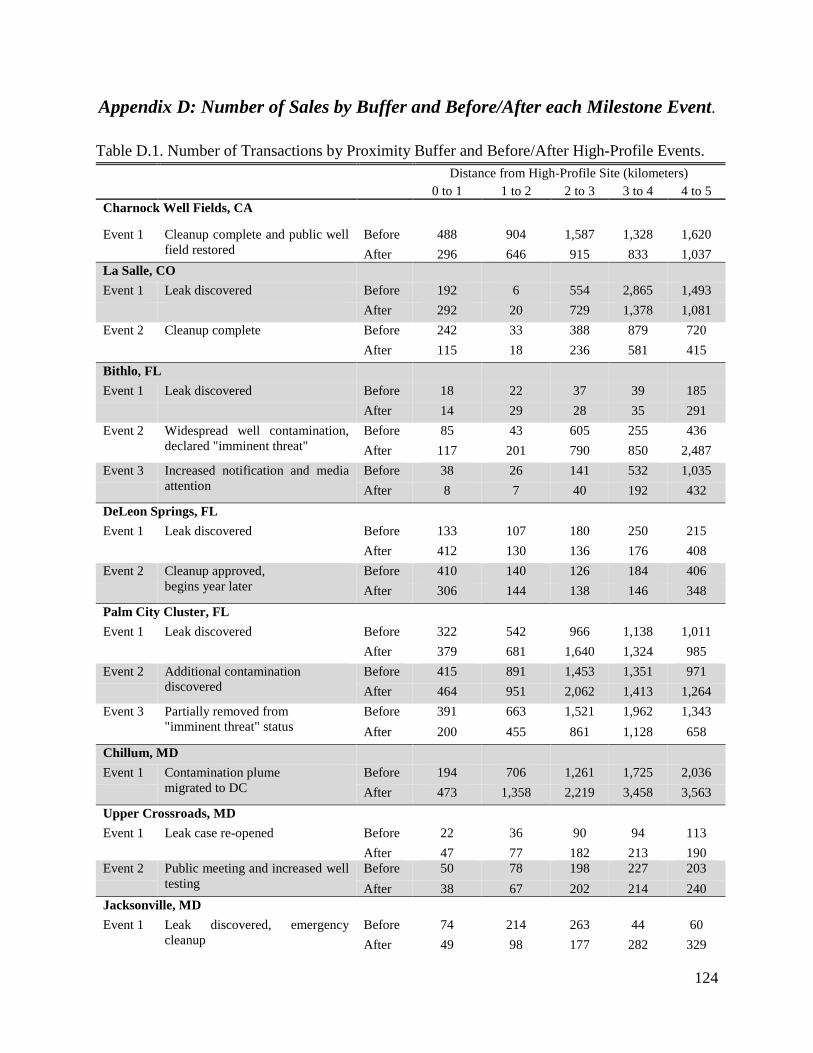
124

Appendix D: Number of Sales by Buffer and Before/After each Milestone Event.

Table D.1. Number of Transactions by Proximity Buffer and Before/After High-Profile Events.


0 to 1 1 to 2 2 to 3 3 to 4 4 to 5

Charnock Well Fields, CA

Event 1 Cleanup complete and public well

field restored

Before 488 904 1,587 1,328 1,620

After 296 646 915 833 1,037

La Salle, CO

Event 1 Leak discovered Before 192 6 554 2,865 1,493

After 292 20 729 1,378 1,081

Event 2 Cleanup complete Before 242 33 388 879 720

After 115 18 236 581 415

Bithlo, FL

Event 1 Leak discovered Before 18 22 37 39 185

After 14 29 28 35 291

Event 2 Widespread well contamination,

declared "imminent threat"

Before 85 43 605 255 436

After 117 201 790 850 2,487

Event 3 Increased notification and media

attention

Before 38 26 141 532 1,035

After 8 7 40 192 432

DeLeon Springs, FL


After 412 130 136 176 408

Event 2 Cleanup approved,

begins year later

Before 410 140 126 184 406

After 306 144 138 146 348

Palm City Cluster, FL


After 379 681 1,640 1,324 985

Event 2 Additional contamination

discovered

Before 415 891 1,453 1,351 971

After 464 951 2,062 1,413 1,264

Event 3 Partially removed from

"imminent threat" status

Before 391 663 1,521 1,962 1,343

After 200 455 861 1,128 658

Chillum, MD

Event 1 Contamination plume

migrated to DC

Before 194 706 1,261 1,725 2,036

After 473 1,358 2,219 3,458 3,563

Upper Crossroads, MD

Event 1 Leak case re-opened Before 22 36 90 94 113

After 47 77 182 213 190

Event 2 Public meeting and increased well

testing

Before 50 78 198 227 203

After 38 67 202 214 240

Jacksonville, MD

Event 1 Leak discovered, emergency

cleanup

Before 74 214 263 44 60

After 49 98 177 282 329

125



After 100 69 113 181 124

Event 2 Notification sent to all residents

within 1/2 mile

Before - - - - -

After 23 30 80 104 109

Hendersonville Corner Pantry, NC


After 29 102 58 151 324

Event 2 Public water line extended Before - - - - -

After 55 176 129 288 563

Montvale, NJ

Event 1 Re-opened (old leak discovered) Before 71 202 276 230 401

After 73 172 191 160 248

Event 2 State mandated cleanup Before - - - - -

After 164 395 409 377 617

Event 3 Widespread vapor concerns,

RP purchased 5 homes

Before 181 396 433 388 569

After 125 300 359 293 489

Suffolk, NY

Northville Industries, NY

Event 1 Cleanup complete Before 74 348 519 1,101 1,370

After 92 364 630 1,182 1,311

Smithtown Exxon-Mobil, NY

Event 1 Leak discovered near

previous release

Before 59 160 199 239 316

After 196 612 726 997 1,159

Event 2 Cleanup complete Before - - - - -

After 83 245 358 417 479

West Hempstead

Event 1 MTBE detected in public water

well

Before 367 785 1,992 2,525 3,636

After 99 199 436 678 957

Event 2 New water supply well installed

Before - - - - -

After 233 477 1,094 1,795 2,358

Pascoag, RI


After 83 190 127 124 115

Tuckahoe, VA


After 136 289 357 491 566

Event 2 Cleanup complete Before - - - - -

After 50 110 143 235 230

Pearl Street Gulf, VT


After 129 106 96 83 257

Note: Color shades denote estimates from the same hedonic regression.