Do Increased Capital Requirements Lead to

Higher Interest Margins? -A Study in the Swedish Banking Sector

Bachelor thesis in Financial Economics (15 credits)

Department of Economics

Lowe Rehnberg & Marcus Wikström Supervisor: Wlodek Bursztyn

June 2014

1

Abstract

This paper examines the impacts of the capital ratios stipulated in Basel III on banks’

interest margins. The Basel III rules were established as a response to the financial

crisis in 2007-2009 when it became obvious that the previously existing rules were

unable to cope with the growing complexity of the financial markets. The four largest

banks in Sweden are analyzed: Nordea, Svenska Handelsbanken, SEB and Swedbank.

The central theoretical backbone is the Modigliani Miller theorem with the presence

of corporate taxes, which states that when a firm’s equity to total assets increases, the

results are higher funding costs. The results of the quantitative study show that

capital ratios calculated using risk-weights do not seem to have a significant effect on

interest margins for the four largest banks in Sweden. However, the Equity Ratio

calculated on total assets, using no risk-weights, has a positive effect on interest

margins in the Swedish banking market. This empirically provides support for the

specialized Modigliani Miller theorem with corporate taxes.

Key Words: Banking, Basel III, Modigliani Miller, Capital Ratio, Capital

Requirements, Interest Margins, Sweden

Table of Contents Introduction 1

Purpose 2 Limitations of the Study 2 Disposition 3

Background 3 Bank Assets and Funding 3 Banking Capital 4 Advantages and Disadvantages with Capital in Comparison to Debt 4 Solvency and Liquidity 6 Basel Accords 7

Basel I and II 7 The Financial Crisis of 2007-2009 8 Basel III 9

Timetable of the Basel III Implementation in Sweden 10 Framework of Basel III 10 Capital Requirements 11 Counter-Cyclicality 11 The Three Pillars of Basel III 12 Liquidity Requirements 13 Major Criticisms Against the Basel Rules 13 Systemic Risk Impact 14

Theory 15 Cost Impact - How Does Basel III Affect Costs for Banks and Society? 15

Factors making debt preferable to capital 15 Factors making capital preferable to debt 18

Methodology 20 Sample 21 Dependent Variable 21

Net Interest Margin 21 Independent Variables 22

Total Capital Ratio 22 Tier 1 Capital Ratio 22 Equity Ratio 22

Control Variables 23 Credit Risk 23 Standard Deviation of the Swedish Interbank Rate Stibor 23 Credit Risk*Stibor 3m SD 23 Liquidity Risk 24 Interbank Ratio 24

1

Year Dummies 24 Regressions 25

Results and Analysis 26 Total Capital Ratio – Regression 1 28 Tier 1 Capital Ratio – Regression 2 28 Equity Ratio – Regression 3 29 Control Variables 30

Conclusion 31

Further Research 32

References 33 Published Sources 33 Internet Sources 35

1

Introduction

The financial crisis that started in the US in 2007-2008 has since then had a massive

effect on the world economy. What led to the crisis was that banks were too fragile

partly due to a strong interconnectedness between the banks while lacking sufficient

capital to absorb the losses. The interconnectedness created a type of domino effect

where one bank’s fall affected several other banks. As a result, a number of banks

became insolvent and the consequences further spread across the banking system

(Acharya et al. 2011). Many banks had been taking excessive risks in different types

of mortgage-backed securities. These were placed in off-balance sheet instruments,

which paved the way for higher leverage and as a consequence, higher risk. When

house prices started to decline and the market lost confidence in these securities, it led

to a breakdown in the financial sector. This spread and affected large parts of the

economy and ultimately state bailouts and guarantees were needed to prevent the

financial sector from collapsing (BIS 2010).

The financial system is still highly interconnected. The interconnectedness causes

systemic risk, which means that there is a risk for the entire banking system. If a bank

is considered systemically important, chances are higher that the bank will be bailed

out in case of liquidity shortage or insolvency. This creates an incentive for banks to

become bigger and gain status as systemically important, thereby making them too

big to fail and removing the threat of bankruptcy. Furthermore, when there is no risk

for bankruptcy, the banks have an incentive to increase their level of risk to become

more profitable through leverage. In times of economic expansion, banks can increase

their profitability through borrowing rather than using its equity (capital). However, in

times of economic contraction, capital is important in order to prevent bankruptcy. If

the bank does not have enough capital in bad times and they experience losses, the

risk is larger that the bank becomes insolvent. The alternatives then are either

bankruptcy or hoping to be bailed out by the government, using taxpayers’ money,

thereby causing a massive cost to society (Admati & Hellwig 2013).

2

The Basel rules aim to make the banking system more stable and reduce the risks,

making the banks have higher capital ratios, adjusting the rules for what is allowed to

be included in the capital of a bank and sharpening the rules for how to calculate risk-

weighted assets (RWA) (Riksbank 2011). The previous Basel-frameworks have

obviously not been sufficient in their role to stabilize the financial markets and as a

response to the financial crisis; the new Basel III rules were implemented starting in

November 2010 and are expected to be fully implemented 2019 (Acharya et al. 2011).

The specialized Modigliani Miller theorem with corporate taxes suggests that the

funding costs decrease for a firm with a higher composition of debt in contrast to

equity (Modigliani & Miller 1958). This implies that higher capital requirements

would lead to higher funding costs. There are several studies suggesting that the

higher funding costs resulting from increased capital ratios, in turn will increase

interest margins (Angbazo 1997) and/or interest rate spreads (Slovik & Cournède

2011). Interest margins are the difference between the banks’ interest income and

interest costs. Interest rate spreads are the difference in lending and borrowing rates.

As a result of Basel III, do increased funding costs for large complex financial

institutions cause the banks to increase their interest margins in order to maintain their

profits?

Purpose The aim of this paper is to empirically test if the capital ratios defined in the Basel III

rules affect a bank’s Net Interest Margins through an increase in funding costs,

focusing on the four main Swedish large complex financial institutions (LCFI).

Limitations of the Study The study will be made in the Swedish banking industry. The four major LCFIs in

Sweden are included in the study over a five-year period reaching from 2009 to the

first quarter of 2014. Only Swedish banks are included in the study, as the ambition is

to be able to generalize the results in the Swedish banking sector. Three different

types of capital ratios will be examined in order to establish if there are differences

between the ratios in the effects on interest margins.

3

Disposition The paper starts with an introduction of the fundamental role of capital in a bank,

after which a brief history of the development of the Basel Committee of Banking

Supervision follows. This leads to the necessity of further development of the rules

after the shortcomings of the previous framework is made clear when investigating

the effects of the financial crisis of 2007-2009. As a result of the crisis, Basel III was

developed. These accords are explained in the following section. The theory concerns

what factors determine a firm’s funding costs and which role the composition of

capital and debt plays in deciding these costs. The methodology presents the statistical

model developed in order to test the theory and in the results and analysis, the

findings are presented. The final part consists of the conclusions and proposals for

further study of the subject.

Background

Bank Assets and Funding In order to fully comprehend the Basel III regulations and its impacts, it is first

beneficial to clarify how banks’ balance sheets i.e. their assets and liabilities (funding)

are constructed and what risks banks are exposed to, potentially causing a bank to fail.

Figure I illustrates a simplified overview of a bank’s assets and funding. The funding

consists partly of shareholders’ equity, which in banking is the primary component of

the bank’s capital, and debt. The debt is divided into deposits, short-term and long-

term debt. The short-term debt is usually the primary debt borrowed in the money

market, which typically implies borrowing from other financial institutions. In other

words, the banking system is closely interlinked. The asset side of the balance sheet

comprises short-term loans, long-term loans, reserves and other investments.

Assets Liabilities

Short-term loans Deposits Long-term loans Short-term debt

Reserves Long-term debt Other investments

Shareholder equity

(Capital) Figure I - A simplified balance sheet of a bank.

4

Banking Capital

What constitutes banking capital is complex. In addition to common stock, other

categories can also be counted as capital e.g. preferred stock and to a limited extent

some types of debt such as subordinated debt with a perpetual or very long-term

maturity (Elliot 2010a). One definition is that capital is the portion of the bank’s

funding which is not legally bounded to be repaid to anyone. Capital is the equity of a

bank’s capital structure and should not be confounded with reserves. An argument

often made by banks is that the costs will increase as the banks are forced to “hold”

more capital in the same way they are forced to hold reserves. This is not a valid

argument since capital and reserves are two different things. The reserve level limits

how much banks can lend by stating a minimum percentage of the aggregate lending

the bank must keep in reserves. If the reserve ratio for example is 5 % this means that

if the bank lends 100 USD to a customer, the bank must keep 5 USD in reserves. In

contrast, capital requirements only states what fraction of the total assets that must

consist of non-borrowed funds instead of debt, which means banks do not need to

hold capital in the same way they need to hold reserves (Admati & Hellwig 2013).

Advantages and Disadvantages with Capital in Comparison to Debt According to the basic Modigliani Miller theorem (MM) (assuming no taxes, no

bankruptcy costs etc.), the value and funding costs of a firm are the same for an

unlevered and a levered firm (Modigliani and Miller 1958). Therefore, leverage

cannot increase the value of the firm. It can however increase its return on equity

(ROE) i.e. the firm’s profitability on the owners’ share of the firm. Imagine buying a

house at a price of 1,000,000 SEK. If you purchase the house using your own capital,

if the house price appreciates 10% and you sell it after one year, you will make 10%

on your down payment. Instead imagine that you are borrowing 850,000 SEK at a 5%

interest rate in order to purchase the same house i.e. you pay 42,500 SEK interest per

year. Your down payment is now 150,000 SEK, thus borrowing 85% of the house

purchase price. The listing below illustrates the return on equity when prices rise or

fall using both leverage (paying 5% interest) and only your own capital to purchase

the house. ROE (given no installment) is defined as the earnings of the price-increase

minus the interest payment divided by the down payment.

5

1. Price rises 10%, no leverage:

2. Price rises 10%, 85% borrowed:

3. Price declines by 10%, no leverage:

4. Price declines by 10%, 85% borrowed:

These equations illustrate the increased sensitivity when a firm is using leverage

rather than capital. Also, the potential losses on total capital are greater than the

potential earnings when exploiting the same level of leverage. In times of economic

expansion, the leverage increases the return on equity but in times of economic

contraction, a larger leverage ratio will increase the losses in relation to equity, which

is made clear in the fourth equation where almost all of the down payment is lost

when the price declines. Please note that this is an example buying a house. Banks

often use higher leverage ratios, thus increasing the sensitivity.

Also note that even if your profitability increases with leverage, the value of the house

is the same in both situations in accordance with MM.

Capital is of great importance when a financial firm falls into distress. The distress

situation can be described as a downward liquidity spiral: When a financial firm with

insufficient capital suffers asset losses, the firm’s funding decreases, forcing the firm

to sell its assets, leading to further funding problems (Brunnermeier & Pedersen

2009). If however, the financial firm would have had a greater level of capital, the

negative spiral could be decelerated. The solvency risk is reduced and the liquidity

risk through risk for runs is also indirectly reduced because depositors and other

creditors tend to be less anxious about their money (Admati & Hellwig 2013). Hence,

illiquidity and insolvency are closely interlinked.

6

Solvency and Liquidity

A financial firm is exposed to mainly two types of risk: Solvency (capital risk) and

liquidity risk. Solvency risk is the risk that the market value of a bank’s assets falls

below its obligations. Liquidity risk, on the other hand, implies that the bank cannot

convert its illiquid assets into cash in order to pay off its obligations (Acharya et al.

2011). Banks and other financial institutions are particularly susceptible to liquidity

risk because of its tendency to hold assets with long-term duration or low liquidity

when, at the same time, their liabilities are highly short-term in nature (Acharya et al.

2011). This is a prerequisite for bank runs i.e. many depositors demand their deposits

back at the same time, while the bank is unable to convert the long-term assets into

cash. One should note that the two types of risk are interlinked in the sense that most

bank runs are triggered by indication of a bank’s insolvency (Admati & Hellwig

2013).

Because of the banking system’s close interconnectedness, when one financial firm

defaults, the losses spread throughout the system leading to aggregate shortfall of

capital. This is partly due to the interconnectedness e.g. that banks borrow from each

other, but also because of herd-behavior i.e. banks tend to hold similar assets

(Acharya et al. 2011). In a broader perspective, this so-called systemic risk may be

viewed as the most important risk since it does not only affect specific banks but

larger parts of the economy. Systemic risk is increased by the phenomenon commonly

known as financial firms being “too big to fail”. This suggests that when a financial

firm becomes sufficiently large and interconnected with other firms, the economy as a

whole could face severe consequences if the firm defaults. As an intervention for

mitigating the risks of the banks being “too big to fail”, governments institute

guarantees protecting financial firms from bankruptcy. These guarantees can serve as

incentives for banks becoming “too big to fail”, meaning that banks strive to become

large in order to receive the guarantees. However, government guarantees can cause

problems in the sense that they create a moral hazard. The guaranteed banks are aware

of their protected financial situation, which can lead to further risk taking even in

financial distress (Turner 2010).

7

Basel Accords When the fairly small German bank Herstatt failed in 1973, the central bank

governors of the G-10 countries observed a need for a new universal banking

supervisory body and established the Basel Committee on Banking Supervision

(BCBS) the following year. Its accords are implemented by the member states (BIS

2010). The first Basel accords were formed by negotiations in the late 1980s leading

to the formulation of Basel I in 1988. The Basel Accords later evolved into Basel II

with more strict requirements and more finely calibrated rules with regards to risks

concerning investments and loans. As a result of the recent financial crisis in 2007-

2009, the shortcomings of Basel II became obvious, leading to the formation of Basel

III. However, some argue that the Basel III rules still are insufficient, in particular in

terms of mitigating the systemic risk (Acharya et al. 2011).

Basel I and II The aim of Basel I was primarily focused on the bank’s capital levels with respect to

its assets in order to mitigate the credit risk. Capital is expressed in different tiers, Tier

1 being the capital consisting mainly of paid-up shares, common stock, preferred

stock and retained earnings. Tier II, on the other hand, consists of less reliable capital

such as subordinated debt. Additionally, the Basel Accords introduced the concept of

risk-weighting the assets. This means that the total assets of the banks are evaluated

and weighted according to their risk. Examples of risk-weights are 0% for cash, 20%

for claims on banks incorporated in the OECD and guaranteed loans and 100% for

claims on the private sector. The concrete measure the Basel Accords mentions is

primarily the Total Capital Ratio (Capital Adequacy Ratio) i.e. Tier I and II capital

divided by the risk-weighted assets (RWA) of the bank. Basel I established

requirements that the Total Capital Ratio should be minimum 8% of the bank’s RWA

of which 4% should be Tier 1 capital (BCBS 1988). Furthermore, Basel II developed

the accords and divided the requirements into three pillars:

1) Bank’s must maintain minimum capital amounts with respect to not only credit risk

but also market and operational risk.

8

2) A framework is provided for managing different types of risks not included in the

first pillar e.g. liquidity risk, legal risk and systemic risk.

3) The third pillar includes requirements for transparency towards shareholders and

clients i.e. the banks are regulated to disclose information. (BIS 2013)

The Financial Crisis of 2007-2009 In the end of 2006, house prices in the US began to decline after a long period of

rising prices, which had made it attractive to buy a house and take on a big mortgage.

Many of these loans were classified as so-called sub-prime loans i.e. loans to people

with lower credit rating (Norberg 2009). Housing prices kept increasing and banks

were willing to provide mortgages without being able to foresee the decline in prices

(Ordeberg 2010). When prices began to decline however, many defaulted on their

loans, which led to problems for the banks that now experienced heavy credit losses

(Acharya et al. 2011). Banks had been selling so-called mortgage backed securities

(MBS) which are securities consisting of several thousands of mortgages which are

put together. The MBSs were thought of low-risk investments as they could absorb

credit losses from a few households due to its diversity. The MBSs were further

converted into Collateralized Debt Obligations (CDO), which are constructed by

purchasing large number of MBSs and repackaging them and selling the new security

(CDOs) (Norberg 2009). In this process, the credit rating of the securities was often

raised making investors believe it was a safer investment than it in reality was. 75 %

of the repackaged CDOs were given the rating AAA although the underlying MBSs

were only rated at a maximum BBB (Grant 2008). As a result, the risks were

implicitly raised within the banking system.

Placing the securities in off-balance sheet vehicles, the banks were able to circumvent

the Basel rules of capital requirements. These off-balance sheet vehicles operate

under different rules and are separated from the bank. If the bank were to buy the

securities, they would have to succumb to the Basel rules and use 8% capital of RWA.

However, with off-balance sheet vehicles, banks only had to use 0,8% capital (Rausa

2004). These structural investment vehicles (SIVs) relied on short-term loans for their

financing. However, in the end of 2007, as the rating institutes began to adjust their

previous ratings downward, investors’ willingness to provide these loans to SIVs

9

declined. The effect was that the banks had to finance these entities themselves,

making them re-appear in the balance sheet. This lead to large costs for the banks and

many went into financial troubles (Norberg 2009). Officially, the 20 largest banks in

the US exhibited capital ratios averaging 11,7 % i.e. well above the Basel

requirements. Of these 20, five failed during the crisis, which indicates that capital

requirements are not the only solution (Acharya et al. 2011).

As the bubble finally burst in the fall of 2008, it was made clear that the

interconnectedness among the financial institutions had created a massive systemic

risk (Acharya et al 2011). The banks had taken massive risks using off-balance sheet

vehicles and because of herd-behavior, most of them had acted similarly and invested

massively in MBS’s and CDO’s, which in the end turned out not to be as safe of an

investment as it was thought to be (Acharya et al 2011).

The effects on the world economy were and still are massive. Many countries went

into recession and the recovery is still continuing. Consequently, it was made clear

that the existing rules for the financial sector were insufficient. As a result of the

crisis, the Basel rules have been reviewed and the new Basel III rules were

implemented starting in 2010. The transition period will then last until 2019 when the

rules are to be fully implemented (Riksbank 2010).

Basel III When the financial crisis of 2007-2009 hit, and the existing Basel II rules were proven

insufficient to provide stability in the banking sector. As a response, the Basel III

accords were implemented, starting in 2010 (Acharya et al. 2011). The objective of

reforming the previously existing Basel II was according to the Basel Committee: “To

improve the banking sector’s ability to absorb shocks arising from financial and

economic stress, whatever the source, thus reducing the risk of spillover from the

financial sector to the real economy” (BIS 2010).

Although the Basel III rules are more ambitious than its predecessors in the pursuit of

achieving stability in the financial sector, some major criticism against the new

accords exist. Some of the most common criticisms are that the required capital ratios

10

are not sufficient and the requirements should have been stricter. Additionally, the

new Basel III rules are most concerned with separate entities and thereby neglecting

the systemic risk for the entire economy (Acharya et al. 2011).

Timetable of the Basel III Implementation in Sweden

Table II - The timetable for implementation of Basel III in Sweden – Illustrates when

the different requirements are to be implemented (Riksbank 2011).

Framework of Basel III Because of the obvious shortcomings of Basel II experienced during the recent

financial crisis, Basel III tries to aim a bit differently. In general, the focus broadens

from mainly emphasizing on capital requirements to focusing on more risk categories

such as liquidity risk and problems with cyclicality. The Basel II did introduce more

risk parameters, the concrete rules however were too basic in design, lacking in

accuracy of how residual risk should be treated (Acharya et al. 2011).

2013 2014 2015 2016 2017 2018 2019 Core Tier 1 Capital

Gradual 3.5%

Gradual 4.0%

Final 4.5%

Tier 1 Capital

Gradual 4.5%

Gradual 5.5%

Final 6.0%

Tier 1+2 Capital

Final 8.0%

Capital Conservation Buffer

Gradual 0.625%

Gradual 1.25%

Gradual 1.875%

Final 2.5%

Liquidity Coverage Ratio

Observation

Observation

Final

Net Stable Funding Ratio

Observation

Observation

Observation

Observation

Observation

Final

11

Capital Requirements The required Total Capital Ratio is increased, ranging from 8% to 10.5% of risk-

weighted assets moving from Basel II to III. Tier 1 capital should constitute 6% of

RWA. Core Tier 1 capital i.e. common equity should constitute 4.5% of RWA.

The forces of the financial crisis also indicated that basing capital requirements on

risk-weighted assets was not flawless since it was fairly easy to manipulate these

weights (Acharya et al. 2011). By introducing an additional type of capital

requirement denoted leverage ratio, which is Tier 1 capital divided by total assets (not

risk weighted), one can put constraints on excess leverage while not taking risk-

weights into account. Additionally, the leverage ratio includes off-balance sheet

exposures.

A capital conservation buffer is established where common equity should constitute

2.5% of RWA, in addition to the other requirements. This means that the Total

Capital Ratio will range from 8 to 10.5% depending on the capital conservation

buffer. In times of stress, this acts as a buffer and is rebuilt in better times.

Counter-Cyclicality Another buffer introduced in Basel III is the countercyclical capital buffer. In addition

to the other capital requirements, a buffer is established ranging from 0% to 2.5% of

core Tier 1 capital. This will mitigate the problems of a negative liquidity spiral since

banks are not obligated to hold as much capital in times of stress (Acharya et al.

2011). Furthermore, in better times, banks need to increase their core capital. This

also serves as a braking effect on credit growth, which in turn results in a deceleration

of the build up of systemic risk (Juks & Melander 2012).

12

The Three Pillars of Basel III

Table III – The three pillars established in Basel II remain when moving into Basel III. The requirements within the pillars are further developed (BIS 2014).

Pillar 1

Pillar 2

Pillar 3

Capital Risk Coverage Containing Leverage

Risk Management and Supervision

Market Discipline

Quality level of capital Greater focus on common equity

Securitizations Requires banks to conduct more thorough credit analyses of externally rated securitization exposures.

Leverage ratio A non-risk based form of capital ratio also including off-balance sheet exposures is added.

Supplemental Pillar 2 requirements: A number of residual risks have been taken into account including risk capturing off-

Revised Pillar 3 disclosures requirements: A focus on disclosures related to off-balance sheet vehicles and securitization.

Capital loss absorption at the point of non-viability Clause that allows relevant authority: write-off or conversion of capital instruments to common shares if the bank is judged to be non-viable. Lets private sector help resolve banking crises in order to reduce moral hazard

Trading book Significantly higher capital for trading and derivatives activities, as well as complex securitizations held in the trading book.

balance sheet items and securitization activities.

Banks must provide disclosure for how regulatory capital ratios are calculated.

Capital conservation buffer Common equity should constitute 2.5% of RWA. In times of stress, this acts as a buffer and is rebuilt in better times.

Counterparty credit risk Significantly strengthening the counterparty credit risk framework i.e. the risk that contract counterparties will not live up to their obligations.

Countercyclical buffer A range of 0-2.5% comprising common equity, higher requirements in better times and lower in times of stress

Bank exposures to central counterparties Trade exposures to a qualifying central counterparty will receive a 2% risk weight.

13

Liquidity Requirements Another important aspect of the Basel III, which is not explicitly explored in this

study, is the concept of liquidity ratios. Two major liquidity ratios have been

introduced in Basel III in order to address problems with liquidity. Their objective is

to make banks more robust in distressed situations and mitigate the risk for bank runs.

1. The liquidity coverage ratio is designed to require the bank’s high-quality liquid

assets, such as cash and government securities, to exceed 100% of its net cash

outflows e.g. outflows in retail deposits over a 30-day time period during a critical

system-wide shock.

2. The net stable funding ratio is more long-term in its approach and addresses

liquidity mismatches. This ratio denotes that the bank’s available amount of stable

funding (e.g. capital and longer-term liabilities) should exceed 100% of its required

amount of stable funding, which is the value of held assets multiplied by a factor

representing the asset’s grade of liquidity (Acharya et al. 2011) (BIS 2013).

Major Criticisms Against the Basel Rules

The Basel III rules were developed as a response to the financial crisis of 2007-2009

when it became clear that the previous Basel II framework was not sufficient to

provide stability in the banking sector. Although the new rules have sharpened the

requirements the banks have to succumb to, major criticisms exist, particularly

concerning the capital requirements and the neglecting of the systemic risk (Admati &

Hellwig 2013). The Basel III accords have received critique regarding the fact that the

rules consider banks separately, thereby failing to address the systemic risk of the

interconnectedness in the banking sector (Acharya et al. 2011).

The new rules also fail to address the problems concerning the shadow-banking sector

that was highly involved in the crisis of 2007-2009 and the possibility for banks to

circumvent the new rules, in a manner described as regulatory arbitrage, still exists.

The focus on the separate firm, rather than the sector as a whole makes it possible for

banks to act as before and put some of its operations off-balance sheet (Acharya et al.

2011).

14

Admati & Hellwig (2013) claim, “the new reforms that are being put in place are far

from satisfactory” regarding the robustness of the banks. The required capital ratio of

10.5% has been deemed insufficient and capital ratios of between 20-30% have been

proposed to prevent future financial crisis and provide stability to the banking sector

(Admati & Hellwig 2013). These much higher capital ratios would help stabilize

banks but proposals of this kind are often met with skepticism from bankers, claiming

that this would lead to increased funding costs (Admati & Hellwig 2013).

The risk weighted assets (RWA) and how these are calculated are problematic since it

is possible for banks to manipulate the risk-weights making it possible to circumvent

the rules. The Basel III rules suffer from the same problems as their predecessors as it

is difficult to follow and regulate the many complex trades in the financial markets,

involving for example insurances such as CDSs. Through different trades, banks are

able to effectively raise their leverage ratio above the stipulated levels without

breaking the actual Basel III rules (Blundell-Wignall & Atkinson 2010).

In summary, the criticism against the new regulation is mainly that the problems that

led to the financial crisis will still not be resolved by the new Basel accords.

Systemic Risk Impact Addressing the systemic risk impact, the changes from the previous Basel II include

that banks should have a certain capital ratio in relation to their systemic importance

(Georg 2011). Large financial institutions that are considered as globally systemically

important financial institutions (G-SIFI) are forced to keep an additional capital buffer

of 1,0-3,5 % of core Tier 1 capital depending on how systematically important the

bank is considered (Schuster et al. 2013)

Some scholars argue that the new accords are not sufficient in targeting systemic risk.

The systemic risk also involves the explicit or implicit guarantees given by

governments to bail banks out in times of stress. As long as these guarantees are

present, banks will have an incentive to gain status as systematically important.

However, the Basel III does not consider government guarantees to a large extent

(Acharya et al. 2011). In order for the requirements to be effective, they must generate

higher costs for the banks than the possible gains from a government bail-out and

thereby effectively removing the incentive to become systemically important and gain

15

status as “too big to fail”. Even if the Basel regulation have taken steps in this

direction with the Basel III accords, the role of government guarantees is largely

neglected and banks still have an incentive to become systemically important (Georg

2011).

Theory Cost Impact - How Does Basel III Affect Costs for Banks and Society? An OECD working paper (Slovik & Cournède 2011) argues that GDP growth levels

will diminish by 0.05 to 0.15 percentage points per annum as an effect of larger loan

interest spreads set by banks. This, in turn, is a direct reaction to increased funding

costs originated from the increased capital requirements. Aside from Slovik and

Cournède (2011), there are several other studies indicating that higher capital ratios

lead to higher interest rate margins (Cosimano and Hakura 2011) (Roger and Vlcek

2011) (Elliot 2009 and 2010b) (Angelini et al. 2011). This conclusion contrasts with

the Basel Committee’s view of the cost effects, instead they argue that changes in a

firms funding should not affect the funding cost (Gual 2011). The theoretical

backbone of this argument is that according to the basic Modigliani Miller theorem

(MM) (Modigliani and Miller 1958), the costs of funding a firm are independent of

the firm’s financing structure. However, it should then be emphasized that this theory

is based on the assumption of frictionless environments, which may not hold in

reality. A common argument is that there are several frictions that will not make the

basic MM model applicable (Jaffee and Walden 2010) (Gual 2011). The following

factors serve to prove that we cannot ascertain that financial structure has no effect on

funding costs.

Factors making debt preferable to capital

1. In levered firms, corporate taxes will affect the bank’s financial status leading to

debt being advantageous in contrast to capital. This situation is explained in the

further developed MM model with corporate taxes. The net income of a company will

determine the corporate tax level of the firm. However, interest rates on loans are tax

deductible. This means a tax-shield will arise when a substantial part of the revenue

16

the taxes are based on is deducted, leading to decreased tax payment compared to that

of an unlevered firm (Hillier et al. 2013 p.419 pp) (Modigliani & Miller 1958).

More formally, the elaborated Modigliani Miller theorem with corporate taxes

(Proposition II) (Modigliani & Miller 1958) shows the factors determining the

funding costs:

where:

= Weighted average funding cost of the firm

=Ratio of equity to total assets

=Cost of equity

=Ratio of debt to total assets

=Cost of debt i.e. interest rates to debt holders

=1-The marginal corporate tax

The equivalent equation for the basic MM without taxes (Proposition II) is the same

as the equation above, except that the term is absent. The difference between

the two equations implies that when corporate taxes are involved, the tax term

decreases the funding cost.

17

Figure IV - Shows the difference of firm value between levered and unlevered firms

when corporate taxes are included. Debt is tax-deductible leading to a larger value of

the levered firm compared to the unlevered after taxes have been paid.

2. Another factor not included in the MM model is the presence of asymmetrical

information. This means that the firm’s shareholders do not have access to the same

information as the managers. This can significantly increase the funding costs. In

contrast to debt, the stock market is highly sensitive to information. One example of

the impacts of asymmetrical information is when raising new equity; this signals that

the firm is in poor condition, even if this is not the case, which can lead to a decrease

of the firm’s market value (Myers and Majluf 1984).

3. Government guarantees will make equity disadvantageous in contrast to debt. This

is because borrowing becomes comparably cheap when the bank to some extent is

secured against the risks of borrowing. Government guarantees protect the firms from

bankruptcy. Since one important downside of debt is the increased risk of bankruptcy,

this risk is therefore diminished because of the guarantees. This also means that the

banks investors demand a lower risk premium, which leads to lower funding costs.

Hence, debt becomes comparably advantageous to capital (Jaffee and Walden 2010).

All-Equity Firm

 Equity    (Capital)    

Taxes  

Levered Firm

Equity  (Capital)  

Debt  

Taxes  

18

Factors making capital preferable to debt

1. Expected bankruptcy costs will decrease as capital levels increase. This is because

of the cushion-effect of greater capital levels i.e. higher capital ratios decrease the

default risk (Gual 2011). However, it should be noted that this factor is at odds with

the previously explained factor. Government guarantees create a moral hazard and

remove the risks of borrowing.

2. When a firm is relatively heavily indebted, new investment opportunities may be

disregarded because of the return of the investment directly going to debt holders

(Jaffee and Walden 2010).

The trade-off theory of capital structure argues that when deciding on an optimal

capital structure, there is a trade-off between the benefits and risks of funding with

debt. Initially, when an all-equity firm starts to borrow, the average funding costs

decrease. However, after a certain point, the present value of bankruptcy costs

supersedes the benefits of the tax shield (Figure V). Formally, this point is where the

marginal costs of financial distress equal the marginal tax shield (Hillier et al. 2013).

One could argue however, that a financial firm that is protected under government

guarantees does not face the same expected level of distress costs. This is because the

firm does not longer face these expected costs by itself. Instead the government

removes the risk from the bank leading to the bank’s funding costs not increasing, see

Figure VI. This could create incentives for the banks to strive for a high debt level.

However, this could be hard to validate empirically. Furthermore, the guarantees

create a moral hazard leading to increased risk-taking by the banks, which causes the

government being exposed to the risk created by the banks.

19

Figure V – Shows the changes in funding costs as debt increases in relation to equity

according to the trade-off theory

Figure VI – It can be argued that when banks are protected under government

guarantees, their expected bankruptcy costs cease to exist, preventing the funding

costs to increase after a certain point.

Some scholars argue that capital is expensive compared to debt because shareholders

require higher returns than debt holders (Admati & Hellwig 2013). In other words,

interest rates on loans are lower than shareholders’ required rate of return. Admati &

Hellwig (2013) criticize this view in two concrete ways: The required rate of return

depends on the level of risk of the investment. The costs of equity cannot be

considered separately without referring to a mix of debt and equity. This statement

means that if a firm has a higher leverage, the stock investment will be higher in terms

of risk. If this is the case, the required rate of return will also be higher. This means

that for a firm with lower leverage, and thus higher capital, the equity investment is

less risky; hence the required rate of return should be lower as well.

-­‐10  

-­‐5  

0  

5  

10  

0   5   10   15   20   25  

Funding    Costs  

Debt  

Trade-­‐Off  Theory  -­‐  Funding  Costs  as  Debt  Increases  

Rwacc  

-­‐10  

-­‐5  

0  

5  

10  

0   2   4   6   8   10   12  Funding  Costs  

Debt  

Possible  Outcome  under  Government  Guarantees  -­‐  Funding  Costs  as  Debt  Increases  

Rwacc  

20

Although the banks’ financial status could benefit from higher debt levels through

tax-shields while circumventing much of the natural risk associated with high debt

levels, the costs of state guarantees are high for taxpayers when banks need to be

bailed out by the government. As an example, the US Trouble Assets Relief Program

(TARP) that was launched in the fall of 2008 cost the government, and hence the

taxpayers, 700 billion USD (Norberg 2009). This is only one of many cases of social

costs following the financial crisis. If the crisis would have been prevented, this

money could have been used to a greater good for society.

Methodology In order to measure the banks’ interest margins, the Net Interest Margin (NIM) is used

as the dependent variable. A fixed effect regression using panel data is advantageous

for analyzing the effect on the Net Interest Margin of the banks. This model is

preferable because it allows us to control for and remove unobserved factors over

time; the regression term is denoted ai. It also makes it possible to study a number of

banks over time and obtain unbiased estimators of the beta-coefficients. To avoid

serial correlation and heteroscedasticity, robust standard errors have been used in the

regressions. The avoidance of serial correlation and heteroscedasticity are one of the

criteria that has to be met to be able to use a fixed effects model, the other is that there

has to be variance in all the independent variables in the regression, as these would

otherwise have been eliminated in accordance with the fundamental function of the

model. Time dummies are included in order to capture omitted time effects on the

dependent variable in the regression; these include several unobserved

macroeconomic effects on interest margins. In order to obtain adequate estimators of

the variables, some of them have been lagged one quarter. A negative aspect of using

lagged variables is the reduced degrees of freedom. However, some of the variables

require lags of one quarter in order for the banks to analyze the changes and respond

by changing the interest margin.

21

Sample The Swedish banking sector is particularly interesting to study because the sector is

comparatively large in relation to the Swedish economy. The banking sector in

Sweden is dominated by four major actors; Nordea, Svenska Handelsbanken, SEB

and Swedbank, which together make up for around 75 % of lending and deposits in

Sweden and are also highly interconnected (Ingves 2011). This is why the research

focuses on these banks. We use quarterly data from 2009 to first quarter of 2014 in

order to be able to observe interesting changes in bank behavior over time in response

to the capital ratios defined in the Basel III rules and banks’ equity ratios not using

risk-weights. However, since the Basel III rules are not fully implemented until 2019

this paper aims to provide an initial analysis. Thus, the final evaluation cannot be

made before we can investigate the effects of the complete implementation. The data

is mostly obtained from Bankscope but also from the Swedish Riksbank.

Furthermore, some of the raw data have then been further elaborated and refined.

These regressions are based on 83 observations. This is because only 4 major actors

heavily dominate the banking market in Sweden. Furthermore, the 5-year time period

was chosen to examine banks’ behavior after the financial crisis and to be able to

observe the adaptation to the Basel III capital requirements and how this affects

interest margins.

Dependent Variable

Net Interest Margin The Net Interest Margin (NIM) is defined as the difference between the bank’s

interest earnings and interest expenses, divided by the amount of interest earning

assets. The NIM should act as an indicator of how much the banks adjust their interest

margin as an effect of costs resulting from capital ratios imposed by the Basel III rules

and/or other factors.

22

Independent Variables

Total Capital Ratio

The Total Capital Ratio measures capital in relation to risk-weighted assets. As

concluded by Slovik and Cournède (2011) as well as the recent Finansinspektion

report (2014), the coefficient is expected to be positive as a result of higher funding

costs, leading banks to increase their interest margins.

Tier 1 Capital Ratio

The Tier 1 Capital Ratio is similar to the Total Capital Ratio with the difference being

that the capital mainly consists of common stocks and retained earnings.

Consequently, the coefficient is expected to be similar to that of the Total Capital

Ratio.

Equity Ratio

The Equity Ratio is used in order to test the capital to total assets without taking risk-

weights into consideration; this is therefore useful in testing the Modigliani Miller

theorem with corporate taxes and to a certain extent the trade-off theory. The Equity

Ratio is similar to the leverage ratio of Basel III in the sense that the capital is

measured in relation to the total assets, not taking risk-weights into account. The

variable coefficient is expected to be positive. This would indicate that an increase of

capital in relation to debt would increase the funding costs, as explained by the MM

proposition II with corporate taxes. Thus the banks are expected to increase their

interest margin. The variable is measured as equity/total assets.

23

Control Variables

Credit Risk

Financial firms with a high share of loans to total assets face an increased risk that

debtors will fail to pay back their loans. Therefore, the variable loans to total assets

ratio is used as a proxy for credit risk, which is the same proxy used by Maudos & de

Guevara (2004). The variable will be lagged because credit risk does not tend to affect

the margins immediately (Valverde & Fernández 2007). Additionally, it is logical to

assume that there is some uncertainty to how much the bank will lend in a certain

period of time. Thus, they do not know how much they have lent until the end of the

period observed. When they do have data at the end of the period they can adjust their

margin decisions accordingly. The assumption behind this variable is that the higher

the risk, the higher the Net Interest Margin, because banks have to be compensated

for the increased risk (Angbazo 1997). Therefore it is expected that the coefficient

will be positive.

Standard Deviation of the Swedish Interbank Rate Stibor

Using the standard deviation of the Stibor rate will generate a good measurement of

the volatility in the interest rates. The standard deviation of the Stibor rate is measured

in three variables with different maturity: 3-months, 1-month and 1-week. The idea of

this is to account for that the banks have different maturities on their assets and

liabilities. The standard deviation is calculated on the mean of the specific quarter on

a daily basis. It is expected that higher volatility in the Stibor rate will lead to an

increased market risk for the banks. This is why the effect is expected to be positive

(Maudos & de Guevara 2004). This variable will have a one quarter lag since the

banks respond to the outcome of the previous risk when they determine their present

Net Interest Margin. It is difficult to observe the market volatility as it happens.

Credit Risk*Stibor 3m SD

The interaction term between credit risk and the standard deviation of the Stibor 3-

month rate is used because it can be expected that the market risk, measured by the

24

standard deviation of Stibor, can have an effect on the credit risk, which in turn will

affect the Net Interest Margin (Maudos & de Guevara 2004). The effect of this

variable is expected to be positive, as a larger risk will cause the bank to increase the

Net Interest Margin. Because of the lag on credit risk and market risk individually,

this is why the interaction term is lagged.

Liquidity Risk

Liquidity risk is measured by dividing the bank’s liquid assets with its deposits and

short term funding. As financial firms can quickly borrow money in the money

market, this variable will not be lagged in the same way as the credit risk.

Furthermore, since banks must have a certain ratio of capital relative to the borrowed

funds, banks that have a large liquidity risk are assumed to increase their Net Interest

Margin in order to increase their capital (Valverde & Fernández 2007). The variable

coefficient is expected to be negative because if the ratio decreases, liquidity risk

emerges, which causes the banks to increase their interest margins.

Interbank Ratio

The Interbank Ratio is measured as the ratio between lending assets and borrowed

assets in the interbank market. If a bank is solid and has a high degree of liquidity, it

is expected that this bank will have a positive ratio as it can lend more than it borrows

from other banks. This will in turn lead the coefficient of the variable to be negative

as a solid bank faces less risk and therefore does not have to increase the Net Interest

Margin in order to increase liquidity.

Year Dummies In order to record unobserved time-varying effects, year dummies are included in the

regression. The year dummies can capture effects such as macro factors that are not

included in the model but still have a significant effect on the Net Interest Margin.

The base year of the year dummies will be 2009 which all unobserved

macroeconomic characteristics will be relative to.

25

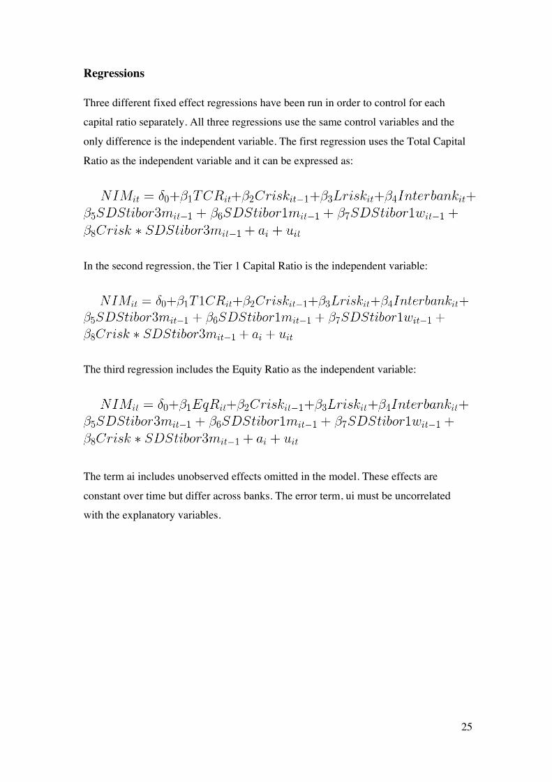
Regressions

Three different fixed effect regressions have been run in order to control for each

capital ratio separately. All three regressions use the same control variables and the

only difference is the independent variable. The first regression uses the Total Capital

Ratio as the independent variable and it can be expressed as:

In the second regression, the Tier 1 Capital Ratio is the independent variable:

The third regression includes the Equity Ratio as the independent variable:

The term ai includes unobserved effects omitted in the model. These effects are

constant over time but differ across banks. The error term, ui must be uncorrelated

with the explanatory variables.

26

Results and Analysis Table VII presents the results of the three regressions using different capital ratios as

dependent variable. Some of the results are interesting and especially worth noticing.

In all three regressions, the control variable Interbank Ratio is significant and has a

negative coefficient, which is the same effect as anticipated. The control variable

Credit-Risk*Stibor3mSD is statistically significant in two of the regressions indicating

that the market risk has an effect on the dependent variable through the credit risk.

The effect is, as anticipated, in both cases positive. Among the independent variables,

only Equity Ratio is proven to have a significant effect on Net Interest Margin. The

R-square value of the three regressions is constant around 0,6, which means each of

the theoretic models has an explaining effect of around 60% of the variance in the Net

Interest Margin.

The results presented account for data from 2009 to the first quarter of 2014. This

means that we cannot draw any conclusive evidence concerning the effects of the

Basel III rules. The complete analysis cannot be made until after the full

implementation in 2019. These results act as an initial analysis of the impacts of

capital requirements imposed by Basel III on interest margins of the four major

Swedish banks.

27

Table VII - Illustrates the three regressions including dependent, independent and

control variables. Standard errors are presented in parentheses. Number of

observations: 83 Significance levels are denoted as: *=10% **=5% ***=1%

Effects of capital ratios on interest margins Dependent variable: Net Interest Margin (1) (2) (3) Total Capital Ratio -0.0213

[0.0205]

Tier 1 Capital Ratio

0.0057

[0.0092]

Equity Ratio

0.0672

[0.0110]**

Credit Risk 0.0085 0.0058 0.0043

[0.0066] [0.0071] [0.0049]

Liquidity Risk -0.0020 -0.0018 -0.0014

[0.0013] [0.0013] [0.0012]

Interbank Ratio -0.0010 -0.0010 -0.0011

[0.0002]** [0.0002]*** [0.0002]**

SD Stibor3m 1.0549 0.9146 0.6299

[0.3974]* [0.5606] [0.6800]

SD Stibor1m -0.3778 -0.1765 -0.4737

[0.7345] [0.7240] [0.4960]

SD Stibor1w 0.4558 0.3467 0.5783

[0.5247] [0.4884] [0.2902]

Credit Risk*SD Stibor3m -0.0173 -0.0159 -0.0100

[0.0040]** [0.0062]* [0.0098]

Year 2010 -0.1188 -0.1165 -0.1211

[0.0369]** [0.0544] [0.0506]

Year 2011 -0.0548 -0.0385 -0.0480

[0.0574] [0.0552] [0.0511]

Year 2012 0.0104 0.0097 -0.0024

[0.0809] [0.0876] [0.0866]

Year 2013 0.0605 0.0753 0.0407

[0.0761] [0.0760] [0.0866]

Year 2014 0.1948 0.0060 0.0217 R-squared (within)

[0.1329] 0.6218

[0.0907] 0.5821

[0.0654] 0.6057

28

Total Capital Ratio – Regression 1 The results of Regression 1, using the total capital ratio as the independent variable,

are presented in Table VII. The coefficient of Total Capital Ratio is insignificant, this

implies that there is no statistical evidence proving a correlation between the capital

ratio based on risk weighted assets and the banks’ interest margins. Regarding the

control variables, the standard deviation of the Swedish interbank rate, capturing the

effect of market risk, shows statistical significance in this regression. Interbank Ratio

and the interaction term between market and credit risk also shows significance. The

results of Regression 1 imply that the examined Swedish banks do not change their

Net Interest Margins when the Total Capital Ratio changes. The reason behind this is

further discussed below. The R-squared of Regression 1 is 0.6218. This implies that

the regression model explains 62.18% of the variation in the dependent variable i.e.

Net Interest Margin.

Tier 1 Capital Ratio – Regression 2 Similar to the regression above, there is no statistical significance in the coefficient of

the Tier 1 Capital Ratio, which is the independent variable of Regression 2 presented

in Table VII. The fact that this variable is not statistically significant indicates that

banks do not change their interest margins following changes in their Tier 1 Capital

Ratio. The reason behind the insignificance in the independent variables of

Regression 1 and Regression 2 respectively might be that banks can change their

capital ratios through adjusting their risk-weighted assets without having to change

their funding i.e. how much debt in relation to capital the bank has (capital structure).

The capital structure is the sole determinant of differences in funding costs according

to the specialized MM model with corporate taxes (Proposition II) and since the

capital structure does not have to change when the ratios based on risk weights do,

this can explain the insignificance in the variable coefficients. The regression model

explains 58.21% of the variation in the Net Interest Margin.

29

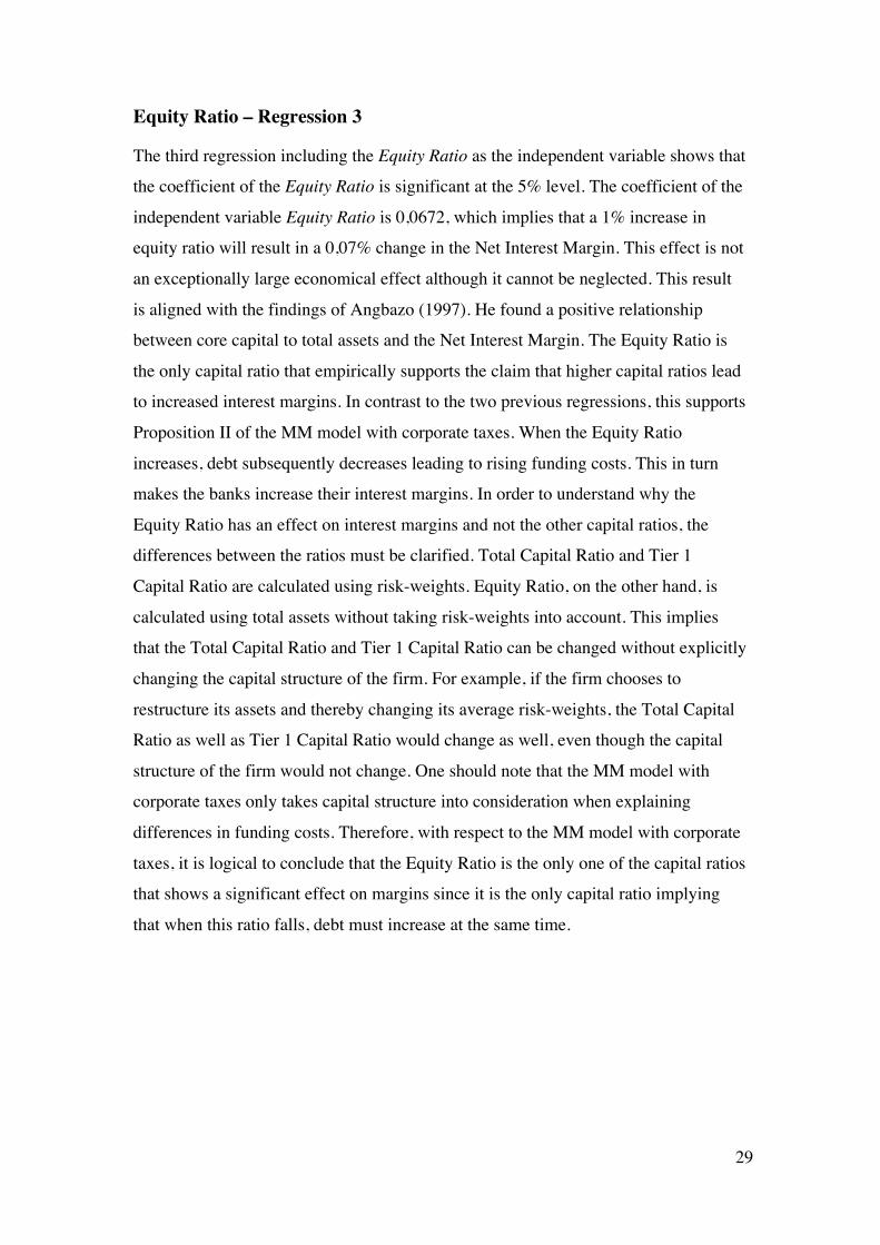
Equity Ratio – Regression 3 The third regression including the Equity Ratio as the independent variable shows that

the coefficient of the Equity Ratio is significant at the 5% level. The coefficient of the

independent variable Equity Ratio is 0,0672, which implies that a 1% increase in

equity ratio will result in a 0,07% change in the Net Interest Margin. This effect is not

an exceptionally large economical effect although it cannot be neglected. This result

is aligned with the findings of Angbazo (1997). He found a positive relationship

between core capital to total assets and the Net Interest Margin. The Equity Ratio is

the only capital ratio that empirically supports the claim that higher capital ratios lead

to increased interest margins. In contrast to the two previous regressions, this supports

Proposition II of the MM model with corporate taxes. When the Equity Ratio

increases, debt subsequently decreases leading to rising funding costs. This in turn

makes the banks increase their interest margins. In order to understand why the

Equity Ratio has an effect on interest margins and not the other capital ratios, the

differences between the ratios must be clarified. Total Capital Ratio and Tier 1

Capital Ratio are calculated using risk-weights. Equity Ratio, on the other hand, is

calculated using total assets without taking risk-weights into account. This implies

that the Total Capital Ratio and Tier 1 Capital Ratio can be changed without explicitly

changing the capital structure of the firm. For example, if the firm chooses to

restructure its assets and thereby changing its average risk-weights, the Total Capital

Ratio as well as Tier 1 Capital Ratio would change as well, even though the capital

structure of the firm would not change. One should note that the MM model with

corporate taxes only takes capital structure into consideration when explaining

differences in funding costs. Therefore, with respect to the MM model with corporate

taxes, it is logical to conclude that the Equity Ratio is the only one of the capital ratios

that shows a significant effect on margins since it is the only capital ratio implying

that when this ratio falls, debt must increase at the same time.

30

Control Variables

The Interbank Ratio is the only one of the control variables that has a statistically

significant effect in all the three regressions. In all models, the effect of the Interbank

Ratio is -0,001 which means that an increase in the Interbank Ratio with one

percentage point will result in a decrease in the banks’ interest margin with -0,001

percentage points. The effects are in line with the expectations. An explanation for

this effect is that if the bank increases borrowing from other banks in relation to

lending, the bank is facing an increased risk. The bank compensates for this risk by

increasing their interest margins. However, although the statistical significance is

especially high in these coefficients, it should be noted that the economical

significance is not very large.

The interaction term between market risk and credit risk implies that there is

significance in two of the regressions. This means that although credit risk is

insignificant by itself, it becomes statistically significant when multiplied by market

risk. This can be interpreted as market risk having an effect on credit risk, which in

turn has a positive effect on interest margins.

The liquidity risk is not significant in any of the regressions. However, one could

argue the Interbank Ratio also is a type of liquidity risk; it only measures another

aspect of the risk. Consequently, this would still support the claim that liquidity risk is

a significant factor in determining interest margins.

Only one of the market risk factors in one of the regressions shows significance in the

effect on interest margins. A reasonable explanation for the lack of significance might

be that the analysis only contains 5 years of observations, which limits the

fluctuations in the variables (Francis & Osbourne 2009).

31

Conclusion Capital ratios calculated using risk-weights do not seem to have a significant effect

on interest margins for the four largest banks in Sweden. However, the Equity Ratio

calculated on total assets, using no risk-weights, has a positive effect on interest

margins in the Swedish banking market. This empirically provides support for the

specialized Modigliani Miller theorem with corporate taxes.

Firstly, it has to be emphasized that the results cannot be interpreted as empirical

evidence of the impacts of Basel III. This is because the implementation of the Basel

III rules is merely in its starting phase. However, the results can give us a guideline as

to what impact fluctuations in capital ratios have on banks’ interest margins of the

largest LCFIs in Sweden.

The results suggest we can find empirical evidence that the MM model with corporate

taxes holds in the Swedish banking sector. It should be stated that the elaborated MM

model suggests that it is the mix of debt and capital (capital structure) that decides the

value of the firm and funding costs, through an emerging tax shield. Accordingly, the

results do imply that changes in the Equity Ratio impact the interest margins of the

banks. These findings are also in line with the study by Angbazo (1997), where a

positive correlation between core capital to total assets and Net Interest Margin is

established. However, the Total Capital Ratio and Tier 1 Capital Ratio defined in

Basel III are based on risk-weights, which means that it is possible for the ratios to

change without actually changing the mix of debt and capital. The results show that

there is no significant correlation between the capital ratios based on risk-weights and

interest margins. In contrast, it can be concluded that capital ratios, where changes in

the capital ratio directly affects debt levels, have a significant effect on interest

margins of the investigated Swedish banks. Furthermore, studies such as Slovik &

Cournéde (2011), Elliot (2009 and 2010) and Angbazo (1997) contribute with an

explanation to the correlation between capital ratios and interest margins being that

the higher funding costs resulting from higher capital ratios, in turn affect the interest

margin.

32

The fact that the regressions merely are based 83 observations in the Swedish banking

market could mean that the results are not generalizable in a broader banking context.

It is suggested that the same study is made internationally after the Basel III rules are

fully implemented in order to achieve a fair conclusion of the impacts of the capital

requirements of Basel III.

Further Research It is of high importance that further studies are made after the implementation process

of Basel III. The results of this study should not be viewed as the impact of the new

Basel rules because the implementation of the Basel III rules to this date only is in its

starting phase. Additionally, macroeconomic analyses can be made in order to

measure the differences in economic growth after the new Basel rules are

implemented. Basel III may contribute to significant changes in the economy.

Therefore, aside from studying the cost effects of more stringent capital requirements,

it is beneficial to explore other effects of Basel III. For instance, studies could be

made on the systemic risk impact of Basel III and further investigate solvency and

liquidity of banks.

This study is focused on the different capital ratios defined in the Basel III rules.

However, another equally important aspect of the rules is the liquidity regulations.

Since this type of regulation differs considerably from capital ratios and that they

form a new type of bank regulation means that it is vital to examine the effects of

these measures as well as the capital ratios,. The effects of the liquidity ratios on

banking behavior and costs for banks and society are suggested as further research.

33

References Published Sources Acharya, Viral V., Cooley, Thomas F., Richardson, Matthew P. & Ingo Walter (2011), ”Regulation Wall Street – The Dodd-Frank Act and the New Architecture of Global Finance”, John Wiley & Sons, 2011 Admati, Anat & Helwig, Martin (2013), ”The Bankers' New Clothes – What´s Wrong with Banking and What to Do about It”, Princeton University Press, 2013 Angbazo, Lazarus (1997), ”Commercial bank Net Interest Margins, default risk, interest-rate risk, and off-balance sheet banking” Journal of Banking & Finance, Vol. 21, (1997) 55-87 Angelini, Paulo, Clerc, Laurent, Cúrdia, Vasco, Gambacorta, Leonardo, Gerali, Andrea, Locarno, Alberto, Motto, Roberto, Röger, Werner, Van den Heuvel, Skander and Vlcek, Jan (2011), ”Basel III: Long-term impact on economic performance and fluctuations”, Bank for International Settlements Working Paper, No. 338, 2011 BCBS (1988), “International Convergence of Capital Measurement and Capital Standards”, Basle Committee on Banking Supervision, July 1988 BIS (2010), ”Basel III: A global regulatory framework for more resilient banks and banking systems”, Bank For International Settlements, December 2010 BIS (2013), ”A brief history of the Basel committee”, Bank for International Settlements, July 2013 Blundell-Wignall, Adrian &Atkinson, Paul (2010), ”Thinking beyond Basel III: Necessary Solutions for Capital and Liquidity”, OECDJournal: Financial Market Trends, Vol. 2010 Issue 1, 2010 Brunnermeier, Markus K. & Pedersen, Lasse Heje (2009), ”Market Liquidity and Funding Liquidity”, The Review of Financial Studies, Vol. 22, No. 6, 2009 Cosimano, Thomas F. & Hakura, Dalia S. (2011), ”Bank Behavior in Response to Basel III: A Cross-Country Analysis”, IMF Working Paper, Vol. 19, No, 119, May 2011 Elliot, Douglas J. (2010a), “A Primer on Bank Capital” The Brookings Institution, January 28, 2010

34

Elliot, Douglas J. (2010b), ”A Further Exploration of Bank Capital Requirements: Effects of Competition from Other Financial Sectors and Effects of Size of Bank or Borrower and of Loan Type”, The Brookings Institution, January 28, 2010 Elliot, Douglas J. (2009), ”Quantifying the Effects on Lending of Increased Capital Requirements” The Brookings Institution, September 21, 2009 Finansinspektionen (2014), ”Capital requirements for Swedish banks” Finansinspektionen Memorandum, May 8, 2014 Francis, William & Osborne, Matthew (2009), ”Band regulation, capital and credit supply: Measuring the impact of Prudential Standards” UK Financial Services Authority, Occational Paper, No 36, September 2009 Georg, Co-Pierre (2011), ”Basel III and Systemic Risk Regulation – What Way Forward?” Working Papers on Global Financial Markets, No. 17, 2011 Grant, James (2008), ”Mr. Market miscalculates: The bubble years and beyond”, Mount Jackson: Axios Press, 2008 Gual, Jordi (2011), ”Capital requirements under Basel III and their impact on the banking industry”, ”la Caixa” Economic Papers, No. 7, Dec 2011 Hillier, David, Ross, Stephen, Westerfield, Randolph, Jaffe, Jeffrey & Bradford, Jordan (2013), “Corporate Finance” McGraw-Hill Education, 2013 Ingves, Stefan (2011), ”Basel III – regulations for safer banking”, Speech given to the Swedish Banker's Association, Stockholm, 10 November 2011 Jaffee, Dwight & Walden, Johan (2010), ”Effekterna av Basel III och Solvens 2 på svenska banker och försäkringsbolag – En jämviktsanalys”, Finansmarknadskommitténs Rapport, No. 3, December 2010 Juks, Reimo & Melander, Ola (2012), ”Countercyclical Capital Buffers as a Macroprudential Instrument” Riksbank Studies, December 2012 Maudos, Joaquín & de Guevara, Juan Fernández (2004), ”Factors explaining the interest margin in the banking sectors of the European Union” Journal of Banking & Finance, Vol. 28, (2004) 2259-2281 Modgliani, Franco & Miller, Merton H. (1958), ”The cost of capital, corporation finance and the theory of investment”, The American Economic Review, Vol. 48, No. 3

35

Myers, Stewart C. & Majluf, Nicholas S. (1984), “Corporate Financing and Investment Descisions – When Firms Have Information That Investors Do Not Have. Journal of Financial Economics 13, (2): 287-221 Norberg, Johan (2009), ”En Perfekt Storm – Hur staten, kapitalet och du och jag sänkte världsekonomin”, Hydra Förlag, 2009 Ordeberg, Thomas (2010), ”Hantering av finanskrisen i EU – rättsliga och institutionella aspekter” In Oxelheim, Lars, Pehrson, Lars & Persson, Thomas (ed.), ”EU och den Globala Krisen” Europaperspektiv 2010, Santérus Förlag, 2010 Rausa, Maurice D. (2004), ”Basel I and the law of unintended consequenses”, Bank Accounting & Finance, Vol. 17 Issue 3, April 2004 Riksbank (2010), “Basel III – skärpta regler för banker” Penningpolitisk rapport, October 2010 Roger, Scott & Vlcek, Jan (2011), ”Macroeconomic Costs of Higher Bank Capital and Liquidity Requirements” IMF Working Paper, Vol. 11, No, 103, May 2011 Schuster, Thomas, Kövener, Felix & Matthes, Jürgen (2013), ”New Bank Equity Capital Rules in the European Union”, IW policy paper, June, 2013 Slovik, Patrick & Cournède, Boris (2011), ”Macroeconomic Impact of Basel III”, OECD Economics Department Working Papers, No. 844, February, 2011 Turner, Adair (2010), “What do banks do? Why do credit booms and busts occur and what can public policy do about it?” The Future of Finance: The LSE Report, London School of Economics, 2010 Valverde & Fernández, Santiago Carbó & Fernández, Fransisco Rodríguez (2007), ”The determinants of bank margins in European banking”, Journal of Banking & Finance 31 (2007) 2043-2063

Internet Sources BIS (2014)” International regulatory framework for banks (Basel III)”, Available (online): http://www.bis.org/bcbs/basel3.htm (26 April 2014) Riksbank (2011) ”Den nya bankregleringen Basel III”, Available (online): http://www.riksbank.se/sv/Finansiell-stabilitet/Finansiella-regelverk/Aktuella-regleringsforandringar/Den-nya-bankregleringen-Basel-III/ (26 April 2014)