do investors overvalue firms with … investors overvalue firms with bloated balance sheets? david...
TRANSCRIPT
DO INVESTORS OVERVALUE FIRMS
WITH BLOATED BALANCE SHEETS?
David Hirshleifer*
Kewei Hou*
Siew Hong Teoh*
Yinglei Zhang*
*Fisher College of Business, Ohio State University. Hirshleifer: [email protected], http://fisher.osu.edu/fin/faculty/hirshleifer/; Hou: [email protected], http://fisher.osu.edu/fin/faculty/hou/; Teoh: [email protected]; Zhang: [email protected]
March 2004 We thank an anonymous referee, David Aboody, Sudipta Basu (JAE 2003 conference discussant), Kent Daniel, Ilia Dichev, S.P. Kothari (editor), Charles Lee, Jing Liu, Stephen Penman, Scott Richardson, Doug Schroeder, Richard Sloan, Jerry Zimmerman, and participants at the Accounting Colloquium at the Ohio State University, and at the Journal of Accounting and Economics 2003 Conference at the Kellogg School, Northwestern University for helpful comments.

DO INVESTORS OVERVALUE FIRMS
WITH BLOATED BALANCE SHEETS?
When cumulative net operating income (accounting value added) outstrips cumulative free cash flow (cash value added), subsequent earnings growth is weak. In this circumstance, we argue that investors with limited attention overvalue the firm, because naïve earnings-based valuation disregards the firm’s relative lack of success in generating cash flows in excess of investment needs. The normalized level of net operating assets is therefore a measure of the extent to which operating/reporting outcomes provoke excessive investor optimism. Consequently, if investor attention is limited, net operating assets will predict negative subsequent stock returns. In our 1964-2002 sample, net operating assets scaled by beginning total assets is a strong negative predictor of long-run stock returns. Predictability is robust with respect to an extensive set of controls and testing methods.
1

1. Introduction
Information is vast, and attention limited. People therefore simplify their judgments
and decisions by using rules of thumb, and by processing only subsets of available
information. Experimental psychologists and accountants have documented that
individuals (including investors and financial professionals) concentrate on a few salient
stimuli (see e.g., the surveys of Fiske and Taylor (1991) and Libby, Bloomfield, Nelson
(2002)). Doing so is a cognitively frugal way of achieving good, though suboptimal
decisions. An investor who values a firm based on its earnings performance rather than
performing a complete analysis of financial variables is following such a strategy.
Several authors have argued that limited investor attention and processing power
causes systematic errors that affect market prices.1 Systematic errors may derive from a
failure to think through the implications of accounting rule changes or earnings
management. However, even if accounting rules and firms’ discretionary accounting
choices are held fixed, some operating/reporting outcomes will highlight positive or
negative aspects of performance more than others.
In this paper, we propose that the level of net operating assets—defined as the
difference on the balance sheet between all operating assets and all operating liabilities—
measures the extent to which operating/reporting outcomes provoke excessive investor
optimism. We will argue that the financial position of a firm with high net operating
assets superficially looks attractive, but is deteriorating, like an overripe fruit ready to
1 See, e.g., Hirshleifer and Teoh (2003), Hirshleifer, Lim and Teoh (2003), Hong, Torous, and Valkanov (2003), Hong and Stein (2003), Pollet (2003), and Pollet and Stellavigna (2003), and the review of Daniel, Hirshleifer and Teoh (2002).
2

drop from the tree. In other words, a high level of net operating assets, scaled to control
for firm size, indicates a lack of sustainability of recent earnings performance.
A basic accounting identity states that a firm’s net operating assets are equal to the
cumulation over time of the difference between net operating income and free cash flow
(see Penman (2002), p.230 for the identity in change form):
∑∑ −=T
0 tT
0 tT Flow Cash FreeIncome OperatingAssets Operating Net (1)
Thus, net operating assets are a cumulative measure of the discrepancy between
accounting value added and cash value added— ‘balance sheet bloat.’
An accumulation of accounting earnings without a commensurate accumulation of
free cash flows raises doubts about future profitability. In fact, we document that high
normalized net operating assets (indicating relative weakness of cumulative free cash
flow relative to cumulative earnings) is a positive indicator of past earnings performance,
but is also an indicator of declining future earnings performance.
If investors have limited attention and fail to discount for this unsustainability, then
firms with high net operating assets will be overvalued relative to those with low net
operating assets. In the long run, such mispricing will on average be corrected. This
implies that firms with high net operating assets will on average earn negative long-run
abnormal returns, and those with low net operating assets will earn positive long-run
abnormal returns.
Net operating assets can also be interpreted as the cumulation over time of the firm’s
operating accruals and investment in operations. To see this, separate free cash flow in
Equation (1) into the difference between cash flow from operations and investment in
operations, and re-arrange the terms. Equation (1) then becomes:
3
,
)
∑∑∑∑
+=
+=T
0 tT
0 t
T
0 t tT
0 tT
InvestmentAccruals Operating
InvestmentFlow Cash -Income (Operating Assets Operating Net (2)
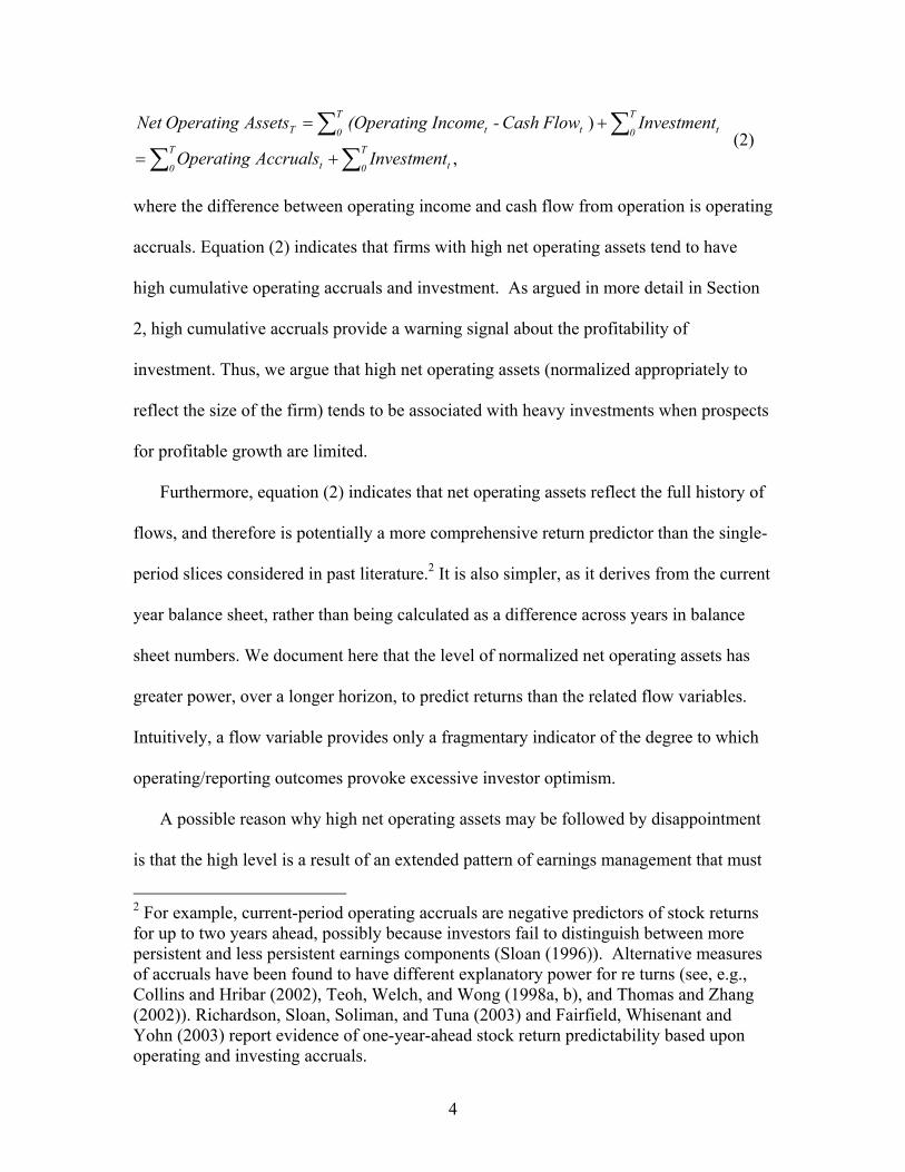
where the difference between operating income and cash flow from operation is operating
accruals. Equation (2) indicates that firms with high net operating assets tend to have
high cumulative operating accruals and investment. As argued in more detail in Section
2, high cumulative accruals provide a warning signal about the profitability of
investment. Thus, we argue that high net operating assets (normalized appropriately to
reflect the size of the firm) tends to be associated with heavy investments when prospects
for profitable growth are limited.
Furthermore, equation (2) indicates that net operating assets reflect the full history of
flows, and therefore is potentially a more comprehensive return predictor than the single-
period slices considered in past literature.2 It is also simpler, as it derives from the current
year balance sheet, rather than being calculated as a difference across years in balance
sheet numbers. We document here that the level of normalized net operating assets has
greater power, over a longer horizon, to predict returns than the related flow variables.
Intuitively, a flow variable provides only a fragmentary indicator of the degree to which
operating/reporting outcomes provoke excessive investor optimism.
A possible reason why high net operating assets may be followed by disappointment
is that the high level is a result of an extended pattern of earnings management that must
2 For example, current-period operating accruals are negative predictors of stock returns for up to two years ahead, possibly because investors fail to distinguish between more persistent and less persistent earnings components (Sloan (1996)). Alternative measures of accruals have been found to have different explanatory power for re turns (see, e.g., Collins and Hribar (2002), Teoh, Welch, and Wong (1998a, b), and Thomas and Zhang (2002)). Richardson, Sloan, Soliman, and Tuna (2003) and Fairfield, Whisenant and Yohn (2003) report evidence of one-year-ahead stock return predictability based upon operating and investing accruals.
4

soon be reversed; see Barton and Simko (2003)3. Alternatively, even if firms do not
deliberately manage investor perceptions, investors with limited attention may fail to
make full use of available accounting information. Thus, the interpretation of net
operating assets that we provide in this paper accommodates, but does not require,
earnings management.4
To test for investor misperceptions of firms with bloated balance sheets, we measure
stock returns subsequent to the reporting of net operating assets. The level of net
operating assets scaled by beginning total assets (hereafter NOA) is a strong and robust
negative predictor of future stock returns for at least three years after balance sheet
information is released. We call this the sustainability effect, because high NOA is an
indicator that past accounting performance has been good but that good performance is
unlikely to be sustained in the future; and that investors with limited attention will
overestimate the sustainability of accounting performance.
A trading strategy based upon buying the lowest NOA decile and selling short the
highest NOA decile is profitable in 35 out of the 38 years in the sample, and averages
equally-weighted monthly abnormal returns of 1.24 %, 0.83% and 0.57%, all highly
3 If investors overvalue a firm that manages earnings upward, the price will tend to correct downward when further earnings management becomes infeasible. Barton and Simko provide evidence from 1993-1999 that the level of net operating assets inversely predicts a firm’s ability to meet analysts’ forecasts. Barton and Simko’s perspective further suggests that low net operating assets constrain firms’ ability to manage earnings downward (in order to take a big bath or create `rainy day’ reserves; see DeFond (2003)). Choy (2003) documents that the Barton and Simko (2003) finding derives from industry variations in net operating assets. 4 A branch of the accruals literature provides evidence that managers take advantage of investor naiveté about accruals to manage perceptions of auditors, analysts, and investors. See, e.g., Teoh, Welch, and Wong (1998a, b), Rangan (1998), Ali, Hwang and Trombley (2000), Bradshaw, Richardson, and Sloan (2000), Xie (2001), and Teoh and Wong (2002).
5
significant, in the first, second and third year, respectively, after the release of the balance
sheet information. In these strategies, each firm’s monthly abnormal returns are obtained
by subtracting its benchmark portfolio returns that has been matched for firm size, book-
to-market, and past 12-month return. Then, either equal- or value-weighted mean returns
are calculated for each NOA decile. The effect remains strong with value weights, and
adjustments for CAPM, and 3- or 4-factor models.
The effect also remains strong after including, in addition to the above controls, the
past one-month returns, three-year returns, and current-period operating accruals using a
Fama-MacBeth methodology. The coefficient on NOA is highly statistically significant,
indicating that the sustainability effect is distinct from the monthly contrarian effect
(Jegadeesh (1990)), the momentum effect (Jegadeesh and Titman 1993), the long-run
winner/loser effect (DeBondt and Thaler (1985), and the accruals anomaly (Sloan
(1996)). Also, since book-to-market and past returns are measures of past and
prospective growth, these controls suggest that the findings are not a risk premium effect
associated with the firm’s growth rate. Furthermore, the ability of NOA to predict returns
is robust to eliminating from the sample firms with equity issuance or M&A activity
exceeding 10% of total assets.
The evidence from the negative relationship between NOA and subsequent returns
suggests that investors do not optimally use the information contained in NOA to assess
the sustainability of performance. A Mishkin test that includes accruals, cash flows, and
NOA as forecasting variables of future earnings and returns is similarly consistent with
investor overoptimism about the earnings prospects of high-NOA firms, although this
nonlinear test requires the trimming of outliers to obtain convergence.
6
Further tests indicate that NOA remains a strong return predictor after additionally
controlling for the sum of the last three years of operating accruals, and the latest change
in NOA. These findings suggest that NOA provides a cumulative measure of investor
misperceptions about the sustainability of financial performance that captures
information beyond that contained in flow variables such as operating accruals or the
latest change in NOA.
Finally, we find that the sustainability effect has continued to be strong during the
most recent 5 years. The sustainability effect was strongest in 1999 coinciding with the
recent boom market, and the predictive power of NOA is robust to the exclusion of this
year. The predictive effect of NOA remained strong even during the market downturn in
2000. Thus, it seems that arbitrageurs were not, in our sample, fully alerted to NOA as a
return predictor.
2. Motivation and Hypotheses
A premise of our hypothesis is that investors have limited attention and cognitive
processing power. Theory predicts that limited attention will affect market prices and
trades in systematic ways. In the model of Hirshleifer and Teoh (2003), information that
is more salient or which requires less cognitive processing is used by more investors, and
as a result is impounded more fully into price. Investors’ valuations of a firm therefore
depend on how its transactions are categorized and presented, holding information
content constant. Reporting, disclosure, and news outcomes that highlight favorable
aspects of the available information set imply overpricing, and therefore negative
subsequent abnormal stock returns. Similarly, outcomes that highlight adverse aspects
imply undervaluation, and positive long-run abnormal stock returns.
7

Several empirical findings address these propositions. There is evidence that stock
prices react to the republication of obscure but publicly available information when
provided in a more salient or easily processed form.5 If different investors allocate limited
attention to different industries, a shock arising in a specific industry will take time to be
impounded in the stocks of firms in other industries. Recent tests have identified industry
lead-lags effects in stock returns lasting for up to two months.6
Hirshleifer and Teoh (2003) predicted that stocks with high disclosed but unreported
employee stock options should on average earn negative long-run abnormal returns, as
should firms with large positive discrepancies between disclosed pro forma versus GAAP
definitions of earnings. Subsequent tests have confirmed these implications (Garvey and
Milbourn (2003), Doyle, Lundholm and Soliman (2003)).
If attention is sufficiently limited, investors will tend to treat an information category
such as earnings uniformly even when, owing to different accounting treatments, its
meaning varies—functional fixation. Several empirical studies examine the effects of
accounting rules or discretionary accounting choices by the firm on market valuations.
Since such treatments affect earnings, they will affect the valuations of investors who use
earnings mechanically, even if the information content provided to observers is held
constant. As discussed in the review of Kothari (2001), the empirical evidence from tests
of such ‘functional fixation’ is mixed.
5 See Ho and Michaely (1988); the empirical tests and debate of the `extended functional fixation hypothesis’ in Hand (1990, 1991) and Ball and Kothari (1991); and Huberman and Regev (2001). 6 See Hong, Torous, and Valkanov (2003) and Pollet (2003)). Pollet and Stellavigna (2003) further find that market prices do not reflect long-term information implicit in demographic data for future industry product demand.
8
The operating accruals anomaly of Sloan (1996) is a natural implication of limited
attention; more processing is required to examine each of the cash flow and operating
accrual pieces of earnings separately than to examine earnings alone. However, this
argument does not explain why investors focus on earnings alone rather than cash flow
alone.
If an investor is going to allocate scarce attention to a single flow measure of value
added, the level of earnings does seem to be the better choice. Past research has shown
that there is information in operating accruals that makes earnings more highly correlated
than cash flow with contemporaneous stock returns (Dechow (1994)). This may explain
why in practice, valuation based on earnings comparables (such as P/E and PEG ratios) is
common. Nevertheless, a pure focus on earnings leads to systematic errors, as it neglects
the incremental information contained in cash flow value-added.
The level of net operating assets can help identify those operating/reporting outcomes
that highlight the more positive versus negative aspects of performance, thereby
provoking investor errors. As discussed in the introduction, it does so by providing a
cumulative measure of the discrepancy over time between accounting value added
(earnings) and cash value added (free cash flow). Cumulative net operating income
measures the success of the firm over time in generating value after covering all
operating expenses, including depreciation. Similarly, cumulative free cash flow
measures the success of the firm over time in generating cash flow in excess of capital
expenditures.
If past free cash flow deserves positive weight, along with past earnings, in a rational
forecast of the firm’s future earnings, then a positive discrepancy between the two
9

indicates that future earnings will decline, and a negative discrepancy indicates that
earnings will increase. An investor who naively forms valuations based upon the
information in past earnings will tend to esteem a firm with high net operating assets for
its strong earnings stream, without discounting adequately for the firm’s relative
weakness in generating free cash flow.
This argument does not require that cumulative free cash flow be a more accurate
measure of value added than cumulative earnings, nor that accounting accruals be largely
noise. What it does require is that cumulative free cash flows contain some incremental
information about the firm’s prospects that is not subsumed by cumulative earnings.
There are at least two reasons why cumulative free cash flow is incrementally
informative to cumulative earnings about future prospects. First, the extent to which
earnings comes from operating accruals rather than cash flow is, empirically, a negative
forecaster of future earnings (e.g. accruals are less persistent than cash flows – Dechow
(1994)). Second, free cash flow additionally reflects the information embodied in
cumulative investment levels, which can affect future firm performance both directly, and
in interaction with operating accruals.
With regard to the first point (the predictive power of the split of earnings between
cash flow and operating accruals), if earnings management is the source of high
cumulative accruals, then these adjustments will add noise to accruals as indicators of the
economic condition of the firm. Even if accruals are informative, this noise reduces the
optimal weight that a rational forecaster would place on past earnings versus cash flows
in predicting future performance.
10

Even if managers do not manage earnings, certain types of problems in the firm’s
operations will tend to increase the cumulative levels of operating accruals, and therefore
will increase higher net operating assets. For example, high levels of lingering, unpaid
receivables will increase the cumulative accruals component of net operating assets.7 To
the extent that high receivables may not be fully realized in cash, they contain adverse
incremental information (beyond that in past earnings) about future earnings. Therefore,
when high cumulative accruals increase net operating assets, an investor who fails to
discount for adverse information about low quality receivables will overvalue the firm.
A mirror image of this reasoning applies to firms with high cumulative deferred
revenues. Customer cash advances not yet recognized as revenues on the income
statement, leads to higher cash flow relative to earnings, and so to lower net operating
assets. So a higher cumulative level of cash advances (owing, for example, to an increase
in demand) contributes to cumulative earnings outstripping cumulative cash flow.
To the extent that high deferred revenues indicate that future earnings will be realized,
they contain favorable incremental information (beyond that in past earnings) about
future earnings. So when high cumulative cash advances increase net operating assets, an
investor who fails to take into account the favorable information contained in the high
deferred revenues will tend to undervalue the firm.
7 Although receivables are short-term, the worst receivables will tend to linger longer, stretching the period during which accruals accumulate. Furthermore, if the lingering of receivables today is indicative of a high failure rate on new receivables in the next year, the problem telescopes forward. Such chaining of bad receivables will tend to elongate the period during which mispricing corrects out.
11

Combining these elements, we see that high cumulative accruals that derive, for
example, from high unpaid receivables or low deferred revenues increase net operating
assets, contain adverse information about future earnings prospects, and contribute to
overvaluation.8 This implies that high net operating assets are associated with low
subsequent stock returns.
We now turn to the second point, that the investment piece of cumulative free cash
flow may provide information about future performance (incremental to the information
contained in earnings), and that this effect can interact with cumulative accruals. By (2),
even a firm that has zero accruals can have high net operating assets. So even without
any interaction between the effects of accruals and investment, a high cumulative level of
investment may indicate low profitability if this level results from empire-building
agency problems and managerial overoptimism. If investors fail to discount fully for
managerial agency problems and biases, they will tend to overvalue firms with high
investment levels. On the other hand, high cumulative investment per se could be a
favorable indicator about investment opportunities. So the effect of investment on
investor misperceptions depends upon a balance of forces.
However, we expect a more systematic conclusion from the interaction between the
effects of cumulative investment and of cumulative accruals. We have argued that a high
level of cumulative accruals is a warning signal for the firm’s future prospects. In such a
8 High net operating assets firms have high past earnings and earnings growth, which on average predicts higher future earnings as well. So we do not argue that future earnings will be lower for high net operating assets firms than for low net operating assets firms, but that the earnings of high net operating assets firms will on average decline, whereas the earnings of low net operating assets firms will increase. Our discussion below concerns the adverse information about firm prospects contained in the investment piece of free cash flow, which is incremental to the favorable information contained in past earnings growth.
12

circumstance, high cumulative investment tends to be a further negative indicator,
because it indicates that the firm is investing heavily at a time when prospects for
profitable growth are limited.
Again, such investment could be a result of managerial agency problems and bias.
More subtly, even positive net present value investment may be associated with future
low profits if this investment is a result of obsolescence of the firm’s fixed assets
(consistent with low unbooked sales). For example, when customer advances decline,
new investment in production facilities may be necessary to maintain product quality and
market share, and hence the preexisting level of the net cash flow stream. In either case,
the combination of high cumulative accruals and high cumulative investment is an
indication that the firm is unlikely to earn increasing profits.
Thus, selecting firms based on high net operating assets exposes the dark side of both
accruals and of investment.9 Rising cumulative accruals can reflect growth and cash to
come, but can also indicate lingering problems in converting accruals into actual cash
flow. High cumulative investment can reflect strong investment opportunities, but can
also reflect overinvestment or a need to replace obsolescent fixed assets. High earnings
and earnings growth per se are indicators of good business conditions and growth
opportunities, and may be associated with high accruals and investment. If strong
earnings are in large part corroborated by strong cash flow, then business conditions are
more likely to be good, high accruals are more likely to be converted into future cash
flow, and investment may add substantial value.
9 Net operating assets can be high even though either cumulative investment or cumulative accruals is low. However, since high net operating assets is the sum of cumulative investment and accruals, it will be statistically associated with high levels of both.
13
However, high net operating assets firms are not selected based on earnings growth
per se, but based on the cumulative sum of investment and accruals. Since the selection
of firms is based on the relative shortfall between cash flow and earnings, the favorable
cumulative earnings performance receives relatively little corroboration from cash flow.
In this situation, the firm’s business environment is likely to be deteriorating. These
weakening business opportunities call forth the dark side of the investment. The high
cumulative investment of these firms is likely to represent either overinvestment, or
replacement of obsolescent fixed assets.
If investors with limited attention fail to recognize the information contained in free
cash flow about future financial performance, they will fail to foresee the financial
deterioration that tends to follow a period of high net operating assets, or the
improvement that tends to follow a period of low net operating assets. They will therefore
overvalue firms with high net operating assets and undervalue firms with low net
operating assets.
Reinforcing intuition is provided by separating depreciation from operating accruals
in Equation (2), NOA can be rewritten as:
∑∑∑ −+=T
0 tT
0 t t
T
0
T
onDepreciatiInvestmentonDepreciati except Accruals Operating
Assets Operating Net
(3)
The last two terms reflect the difference between cumulative investment and cumulative
depreciation. For a firm in a zero-growth steady state, current investment is equal to
current depreciation, so the latest change in net operating assets is equal to the non-
depreciation operating accruals. Thus, a firm with high net operating assets is likely to be
a growing firm, in the sense that cumulative investment has been higher than cumulative
14
depreciation, and to have high non-depreciation accruals. This alternative decomposition
confirms the intuition discussed earlier that scaled net operating assets proxies both for
misinterpretations relating to investment activity and to operating accruals.10
Finally, by Equation (2), firms with high net operating assets will tend to have high
cumulative past investment. These firms may have generated high internal cash flow. If
the investment exceeded internally generated cash, they must have financed some of this
investment through external finance. It is therefore useful to verify whether any relation
between scaled net operating assets and subsequent stock returns is incremental to the
new issues puzzle of Loughran and Ritter (1995). We describe such tests in Subsection
4.2.
3. Sample Selection, Variable Measurement, and Data Description
Starting with all NYSE-AMEX and NASDAQ firms in the intersection of the 2002
COMPUSTAT and CRSP tapes, the sample period spans 462 months from July 1964
through December 2002. To be included in the analysis, all firms are required to have
sufficient financial data to compute accruals, net operating assets, firm size, book-to-
market ratios, and 12-month return momentum. An initial sample of 1,625,570 firm-
month observations is available for the Fama-MacBeth monthly cross-sectional
regressions and the characteristics portfolio-matching analyses. The different test
methods impose varying restrictions depending on the controls such as past returns over
various horizons.
10 In the decomposition of equation (2) the latest change in net operating assets is equal to the sum of current operating accruals and current investment. To the extent that net operating assets is a proxy for growth, any ability of scaled net operating assets to predict returns can reflect risk rather than market inefficiency. It is therefore important in empirical testing to control for growth-related risk measures.
15

3.1 Measurement of NOA, Earnings, Cash Flows, and Accruals
Scaled net operating assets (NOA) are calculated as the difference between
operating assets and operating liabilities, scaled by lagged total assets, as:
NOAt = (Operating Assetst − Operating Liabilitiest) / Total Assetst-1 (4)
Operating assets are calculated as the residual from total assets after subtracting financial
assets, and operating liabilities are the residual amount from total assets after subtracting
financial liabilities and equity, as follows:
Operating Assetst = Total Assetst - Cash and Short-Term Investmentt (5)
Operating Liabilitiest = Total Assetst - Short-Term Debtt - Long-Term Debtt
- Minority Interestt - Preferred Stockt - Common Equityt . (6)
Table 1 provides the associated Compustat item numbers. We also consider an alternative
net operating asset calculation in subsection 4.1.3 because some items are inherently
difficult to classify as either operating or financing.
The accounting firm performance variables, Earnings and Cash Flows, are
defined respectively as income from continuing operations (Compustat#178)/lagged total
assets, and as Earnings – Accruals. The latter variable is operating accruals, and is
calculated using the indirect balance sheet method as the change in non-cash current
assets less the change in current liabilities excluding the change in short-term debt and
the change in taxes payable minus depreciation and amortization expense, deflated by
lagged total assets,
Accrualst = [(∆Current Assetst - ∆Casht) - (∆Current Liabilitiest - ∆Short-term Debtt
- ∆Taxes Payablet) - Depreciation and Amortization Expenset]/Total Assetst-1. (7)
16

As in previous studies using operating accruals prior to SFAS #95 in 1988, we use this
method to ensure consistency of the measure over time, and for comparability of results
with the past studies. We include Accruals and the most recent change in NOA scaled by
beginning total assets as control variables to evaluate whether NOA provides incremental
predictive power for returns.
When calculating net operating assets and operating accruals, if short-term debt,
taxes payable, long-term debt, minority interest, or preferred stock has missing values, we
treat these values as zeroes to avoid unnecessary loss of observations. Because we scale
by lagged assets, the Earnings variable reflects a return on assets invested at the
beginning of the period. The stock return predictability that we document remains
significant when we scale by ending instead of beginning total assets, scale by current or
lagged sales, and impose a number of robustness data screens such as excluding firms in
the bottom size deciles or stock price less than 5 dollars.
3.2 Measurement of Asset Pricing Control Variables
Following the recommendation of Daniel, Grinblatt, Titman and Wermers (1997),
we use the characteristics approach for the asset pricing control variables in predicting
returns. Size is the market value of common equity (in millions of dollars) measured as
the closing price at fiscal year end multiplied by the number of common shares
outstanding. The book-to-market ratio is the book value of common equity divided by
the market value of common equity, both measured at fiscal year end.
In addition to these controls, we also include controls for one month-reversal, 12-
month momentum, and three-year reversal, all measured relative to the test month t of
returns. Ret(-1:-1) is the return on the stock in month t-1. Ret(-12:-2) is the cumulative
17
return between month t-12 and month t-2. Finally, Ret(-36:-13) is the cumulative return
between month t-36 and month t-12. Thus, the return control variables are updated each
month as the Fama-MacBeth cross-sectional regressions roll forward in time. The NOA,
Accruals, Size and Book-to-market variables, however, are only updated every 12
months. In addition to these controls, we also report results after additional adjustments
for the CAPM, the Fama-French 3-factor model, and the Carhart (1997) 4-factor model
which includes a momentum factor.
3.3 Summary Statistics of Data Characteristics
Table 1 describes the mean and median values for selected same-period
characteristics of the sample by NOA deciles. Firms are ranked annually by NOA and
sorted into ten portfolios. Net operating assets vary from about a median of 25% of
lagged total assets in the lowest NOA decile to about 150% in the highest NOA decile.
This suggests that high NOA firms are likely to have experienced recent very rapid
growth, and opens the possibility that investors may have misperceived the sustainability
of this growth.
Table 1 reports that Low NOA firms experienced recent poor earnings
performance while high NOA firms experienced recent good earnings performance;
earnings varies monotonically from a median of −0.5% for NOA Decile 1 to a median of
14.4% for NOA decile 10. This difference in performance is driven by large differences
in Accruals across extreme NOA deciles. Accruals increase monotonically across NOA
deciles from a large negative 8.6% for NOA decile 1 to a large positive 13.8% for NOA
decile 10. Operating Cash Flows do not vary monotonically across deciles. NOA decile
10, however, has significantly lower Cash Flows than all other deciles. NOA decile 1’s
18
Cash Flows are similar to those of NOA decile 8 and 9, and are slightly lower than the
Cash Flows in deciles 2 through 7, which are quite similar to each other.
The high level of Earnings for NOA decile 10 despite its extreme low level of
Cash Flows reflects the extremely high Accruals in NOA decile 10. Similarly, the
extreme negative accruals for NOA decile 1 contribute to the portfolio’s low Earnings
despite its moderate level of Cash Flows.
Our hypothesis concerns investors failing to attend sufficiently to the cumulative
history of accruals and investment. Table 1 reports short-term trends in Earnings in
relation to NOA. These are the current period change in Earnings and the next period
change in Earnings. The low-NOA deciles 1 and 2 experience the worst current decline in
Earnings, and achieve amongst the highest turnaround in Earnings in the next period,
with the highest rebound occurring in NOA decile 1. NOA decile 10, acting like a mirror
reflection, does well previously and subsequently does poorly. Thus, the behavior of
earnings before and after NOA sorting dates is as hypothesized. If, in addition, investors
ignore the fact that NOA provides information about reversals in earnings growth, NOA
will predict future abnormal returns.
Turning to stock market characteristics, Table 1 indicates that extreme (both high
and low) NOA firms have the smallest size measured by either book value of equity or
market value of equity; the lowest book-to-market ratios; and the highest betas. Thus, the
extreme deciles seem to be small, possibly high growth or are overvalued, and risky
firms. It is therefore essential to carefully control for risk in measuring abnormal returns.
Panels C and D provide summary statistics on the components of NOA. All
components contribute substantially to variations in NOA, with an especially strong
19
contribution coming from SAsset in decile 10.
Put Table 1 about here.
Table 2 reports the correlations between NOA, the variable of interest, and the
performance measures and firm characteristics. NOA is persistent; the correlation
between NOA and next period NOA is positive and significant. As expected from the
identity in equation (2), NOA and Accruals are positively correlated.
Also consistent with Table 1 findings, the Spearman correlation indicates that
NOA is positively correlated with Earnings, and current period change in Earnings, and is
negatively associated with Cash Flows and next period change in Earnings. Because of
outliers, the Pearson and Spearman correlations are of the opposite sign for NOA with
Earnings, and with current period change in Earnings. After trimming the extremes at
0.5% the sign of Pearson correlations match the sign of the Spearman correlations. While
Table 1 shows similar characteristics in terms of size, beta, and book-to-market for
extreme levels of NOA relative to the middle deciles, the correlations indicate that NOA
is negatively correlated with beta and positively correlated with firm size. The correlation
with book-to-market is positive for the Spearman and negative for the Pearson tests.
Put Table 2 about here.
3.4 Industry Distribution Across NOA Deciles
Table 3 reports the industry distribution of our sample across NOA deciles pooled
across all sample years. Each decile is widely represented by all the two-digit SIC codes.
Following Fama-French (1992), industry (four digit SIC) codes are grouped into fourteen
industry groups. Panel A reports the percentage of firms in each industry group for each
NOA decile. Comparing across NOA deciles, the extreme NOA deciles (1 and 10) have a
20
relatively lower presence in the Food, Textile, Chemicals, and Durables industry groups.
The extreme NOA deciles also have a higher presence in the Mining and Construction,
Transportation, and Computers industry groups. In addition, NOA decile 1 has a
relatively high presence in the Pharmaceuticals and Financials groups, and a relatively
lower presence in the Extractive, Utilities, Retail, and Services groups. NOA decile 10
has a relatively higher presence in the Extractive and Utilities industry groups.
Panel B reports the percentage of firms in each NOA decile within each industry
group. Looking across NOA deciles, the extreme NOA deciles (1 and 10) have a
relatively larger presence in Mining and Construction, Computers, and Financials
industry groups. Low NOA deciles additionally have a larger presence among
Pharmaceuticals, and Transportation, and high NOA deciles have a larger presence
among Agriculture, Extractive, and Utilities industry groups. Given the industry
variation in NOA noted here, we have verified that our main findings remain strong when
we industry-demean our net operating assets measure (results not reported; see Zhang
(2004) for an industry study on NOA).
Put Table 3 about here.
4. The Sustainability Effect
We have hypothesized that a high level of net operating assets is an indicator of
strong past earnings performance, but also of deteriorating future financial prospects. We
have also hypothesized that investors with limited attention neglect this adverse indicator,
leading to stock return predictability. We first evaluate these hypotheses by presenting
the time profile of accounting and stock return performance in the periods surrounding
21

the sorting year by NOA deciles. We then test the ability of NOA to predict stock returns
controlling for standard asset pricing variables and accounting flow variables.
4.1 Time Trends in Earnings and Returns for Extreme NOA Deciles
Figure 1 describes the time series means of Earnings and annual raw buy-and-
hold stock returns for the extreme NOA deciles 1 and 10. Earnings for high NOA firms
hit a peak—and for low NOA firms a trough—in the conditioning year. High NOA is
associated with upward trending Earnings over the previous several years. This upward
trend sharply reverses after the conditioning year, creating a continuing downward
average trend in Earnings. Low NOA is associated with a mirror-image trend pattern.
From five years prior to the conditioning year, average Earnings uniformly trends down.
From the sorting year onwards, average Earnings uniformly trends upwards.
In general, behavioral accounts of over-extrapolation of earnings or sales growth
trends involve a failure to recognize the regression phenomenon, so that forecasts of
future earnings are sub-optimal conditional on the past time series of earnings.
Conditional on high NOA, earnings growth does not just revert to a normal, slower rate,
it turns sharply negative. An investor who, owing to limited attention, neglects the
information contained in NOA for future earnings is in for a rude surprise. Conditional on
NOA, his forecast errors are severe even if he optimally processes the past time series of
earnings, and has no general propensity to overextrapolate earnings trends.
Average Earnings is uniformly higher for high NOA firms than for low NOA
firms, which reflects the respective glory or disgrace of their past. As a result, even
though high NOA predicts a sharp drop in earnings, cross-sectionally high NOA need not
22
predict lower future Earnings across firms. This depends on the balance between the
time-series and the cross-sectional effect.
Do high NOA firms, as hypothesized, earn low subsequent returns? The annual
raw returns of high NOA versus low NOA firms display a dramatic cross-over pattern
through the event year. High NOA firms earn higher returns than low NOA firms before
the event year, and lower returns after. As the event year approaches, the (non-
cumulative) annual returns of high NOA firms climb to about 35% in year –1, but the
returns are under 5% in year +1. Low NOA firms somewhat less markedly switch from
doing poorly in year –1 to well in year +1. Even as far as 5 years after the event year,
high NOA firms are averaging annual returns lower than those of low NOA firms. This
longer term difference in raw returns in post-event years 3-5 may reflect the difference in
size and beta that was noted in Table 2 between the extreme NOA deciles.
4.1 Are High- NOA Firms Overvalued? Abnormal Returns Tests
4.1.1 Abnormal Returns by NOA Deciles
To test the sustainability hypothesis, it is important to control for risk and other
known determinants of average returns. Table 4 reports the average returns of portfolios
sorted on NOA as defined in Section 2. Every month, stocks are ranked by NOA, placed
into deciles, and the equal-weighted and value-weighted monthly raw and characteristic
adjusted returns are computed. We require at least a four-month gap between the
portfolio formation month and the fiscal year end to ensure that investors have the
financial statement data prior to forming portfolios. The average raw and characteristic-
adjusted returns and t-statistics on these portfolios, as well as the difference in mean
returns between decile portfolio 1 (lowest ranked) and 10 (highest ranked), are reported.
23
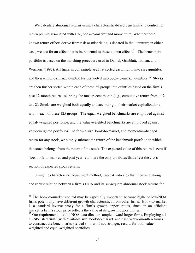
We calculate abnormal returns using a characteristic-based benchmark to control for
return premia associated with size, book-to-market and momentum. Whether these
known return effects derive from risk or mispricing is debated in the literature; in either
case, we test for an effect that is incremental to these known effects.11 The benchmark
portfolio is based on the matching procedure used in Daniel, Grinblatt, Titman, and
Wermers (1997). All firms in our sample are first sorted each month into size quintiles,
and then within each size quintile further sorted into book-to-market quintiles.12 Stocks
are then further sorted within each of these 25 groups into quintiles based on the firm’s
past 12-month returns, skipping the most recent month (e.g., cumulative return from t-12
to t-2). Stocks are weighted both equally and according to their market capitalizations
within each of these 125 groups. The equal-weighted benchmarks are employed against
equal-weighted portfolios, and the value-weighted benchmarks are employed against
value-weighted portfolios. To form a size, book-to-market, and momentum-hedged
return for any stock, we simply subtract the return of the benchmark portfolio to which
that stock belongs from the return of the stock. The expected value of this return is zero if
size, book-to-market, and past year return are the only attributes that affect the cross-
section of expected stock returns.
Using the characteristic adjustment method, Table 4 indicates that there is a strong
and robust relation between a firm’s NOA and its subsequent abnormal stock returns for
11 The book-to-market control may be especially important, because high- or low-NOA firms potentially have different growth characteristics from other firms. Book-to-market is a standard inverse proxy for a firm’s growth opportunities, since, in an efficient market, a firm’s stock price reflects the value of its growth opportunities. 12 Our requirement of valid NOA data tilts our sample toward larger firms. Employing all CRSP-listed firms (with available size, book-to-market, and past twelve-month returns) to construct the benchmarks yielded similar, if not stronger, results for both value-weighted and equal-weighted portfolios.
24
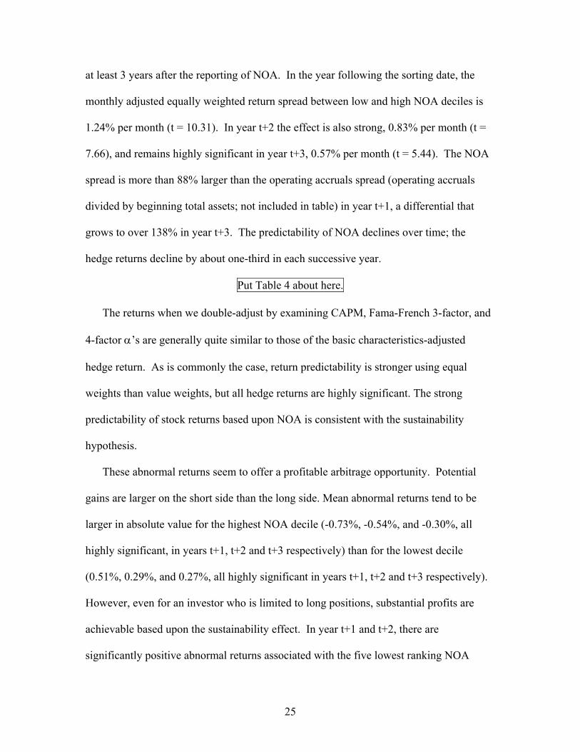
at least 3 years after the reporting of NOA. In the year following the sorting date, the
monthly adjusted equally weighted return spread between low and high NOA deciles is
1.24% per month (t = 10.31). In year t+2 the effect is also strong, 0.83% per month (t =
7.66), and remains highly significant in year t+3, 0.57% per month (t = 5.44). The NOA
spread is more than 88% larger than the operating accruals spread (operating accruals
divided by beginning total assets; not included in table) in year t+1, a differential that
grows to over 138% in year t+3. The predictability of NOA declines over time; the
hedge returns decline by about one-third in each successive year.
Put Table 4 about here.
The returns when we double-adjust by examining CAPM, Fama-French 3-factor, and
4-factor α’s are generally quite similar to those of the basic characteristics-adjusted
hedge return. As is commonly the case, return predictability is stronger using equal
weights than value weights, but all hedge returns are highly significant. The strong
predictability of stock returns based upon NOA is consistent with the sustainability
hypothesis.
These abnormal returns seem to offer a profitable arbitrage opportunity. Potential
gains are larger on the short side than the long side. Mean abnormal returns tend to be
larger in absolute value for the highest NOA decile (-0.73%, -0.54%, and -0.30%, all
highly significant, in years t+1, t+2 and t+3 respectively) than for the lowest decile
(0.51%, 0.29%, and 0.27%, all highly significant in years t+1, t+2 and t+3 respectively).
However, even for an investor who is limited to long positions, substantial profits are
achievable based upon the sustainability effect. In year t+1 and t+2, there are
significantly positive abnormal returns associated with the five lowest ranking NOA
25
portfolios. Significant abnormal returns are achievable using the four lowest ranked NOA
portfolios in year t+3 as well. In contrast (results not reported), in this sample pure long
trading is not profitable based upon the operating accruals anomaly.
Figure 2 Panel A graphs the equally-weighted profits from the trading strategy by
taking a long position in NOA decile 1 and a short position in NOA decile 10 broken
down by year. The strategy is consistently profitable (35 out of 38 years), with the loss
years occurring prior to 1973. The sustainability effect is robust with respect to the
removal of the strongest year, 1999. The general conclusions for value-weighted returns
in Panel B are similar, though not as uniformly consistent. In both panels, the abnormal
profits are substantially larger in recent years.
Put Figure 2 about here.
The NOA profits compare favorably with those from a strategy based on going long
in the lowest operating accruals deciles and taking short positions in the highest operating
accruals deciles. For example (not reported in tables), the equally-weighted profits from
an NOA strategy beat the profits from an operating accruals strategy in 28 out of 38
years. The number of years of higher profits is more evenly split for value-weighted
profits. However, for both equal and value-weighted results, NOA performs much better
than Accruals during the last 5 years; the accruals strategy yielded significant losses in
2000, 2001, and 2002. The greater predictive power of NOA suggests, as proposed in
Section 2, that it is a better proxy for investor misperceptions, because it reflects balance
sheet bloat more fully. In particular, NOA reflects a cumulative effect rather than just the
current-period flow; and, reflects past investment as well as past accruals. It thereby
provides a more complete measure of the discrepancy between past accounting value
26
added and cash value added.
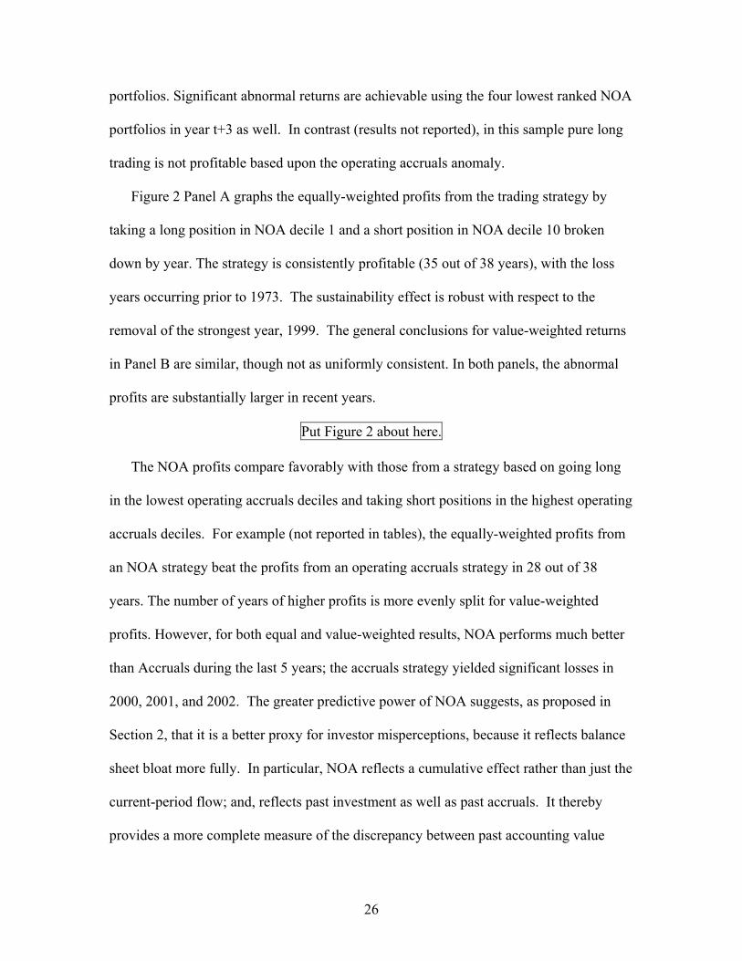
4.1.2 Fama-MacBeth Monthly Cross-Sectional Regression Method
In studies that claim to document how investor psychology affects stock prices,
there is always the question of whether the results derive from some omitted risk factor,
and how independent the findings are from known anomalies. By applying the Fama-
MacBeth method, we evaluate the relation between NOA and subsequent returns with an
expanded set of controls, which consist of momentum, size, and book-to-market; the
short-term one-month contrarian effect, and (by using returns from month –36 to –13) the
long-run winner/loser effect.
Table 5 Panels A, B, and C respectively describe the relation of conditioning
variables and NOA, to returns one year, two year and three years in the future. Model 1
includes standard asset pricing controls, and Model 2 additionally includes the operating
accruals variable. The coefficients confirm the conclusion of past literature that these
variables predict future returns.
Put Table 5 about here.
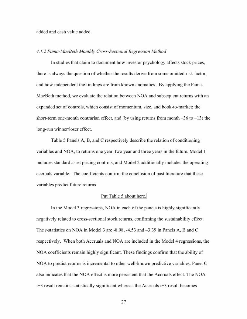
In the Model 3 regressions, NOA in each of the panels is highly significantly
negatively related to cross-sectional stock returns, confirming the sustainability effect.
The t-statistics on NOA in Model 3 are -8.98, -4.53 and –3.39 in Panels A, B and C
respectively. When both Accruals and NOA are included in the Model 4 regressions, the
NOA coefficients remain highly significant. These findings confirm that the ability of
NOA to predict returns is incremental to other well-known predictive variables. Panel C
also indicates that the NOA effect is more persistent that the Accruals effect. The NOA
t+3 result remains statistically significant whereas the Accruals t+3 result becomes
27

insignificant.
4.1.3 Robustness of the Sustainability Effect
NOA in Table 5 is measured using the residual from total assets after subtracting
selected financial assets to obtain operating assets and the residual from total assets after
subtracting equity and financial liability items. This may inadvertently omit operating
items or include financing items. For example, operating cash is often lumped together
with short-term investments and so is omitted from our NOA measure. Some items could
be viewed as either operating or financing. For example, long-term marketable securities
can be sold in the short-term if a cash need arises, and therefore can behave like a
financing rather than an operating item.13 As a robustness check, we consider an
alternative measure, NOA_alt, in which we specifically select for operating asset and
operating liability items. Following Fairfield, Whisenant and Yohn (2003), operating
assets include: accounts receivables, inventory, other current assets, property, plant and
equipment, intangibles, and other long-term assets. Operating liabilities include accounts
payable, other current liabilities, and other long-term liabilities. Table 6 notes contain the
specific Compustat item numbers.
Put Table 6 about here.
Panel A of Table 6 indicates that the two measures of NOA are very similar. The
means, medians, and standard deviations are almost identical, and their correlations with
each other are very high. Thus, not surprisingly, all the results of Tables 4 and 5 are
confirmed using NOA_alt in Table 6 Panels B and C.
13 Goodwill can be viewed as either an operating accrual or an investment. However, NOA includes both operating accruals and investment, so we include goodwill as part of NOA.
28
Panel B reports the hedge profits from the NOA_alt trading strategy calculated
from the characteristics-adjusted portfolio benchmark returns, and alphas from double-
adjusting further using the CAPM, the Fama-French 3-factor, or 4-factor models. For
brevity, only the year +1 monthly profits are reported. All the equally-weighted and
value-weighted hedge returns are statistically significantly positive, confirming the
robustness of Table 4 findings. Similarly, Panel C Fama-Macbeth regression results
confirm that NOA is a robust predictor of abnormal returns, and the NOA effect is
incremental to the operating accruals and other financial anomalies.
4.2 Does NOA Return Predictability Derive from Other Sources?
An alternative to the sustainability hypothesis is that the NOA captures some
known anomaly distinct from the return predictors we have controlled for in previous
tests. For example, the predictive power of NOA might derive from current period
operating accruals (Sloan (1996)) or from the issuance of new equity. To investigate
these and other possibilities, in Table 7 we examine the predictive power of different
components of NOA for one-year-ahead returns. The Fama-Macbeth regressions of Table
5 are now run using alternative decompositions of NOA.
NOA is the cumulative sum of operating accruals and cumulative investment
(equation 2). Thus in addition to current period operating accruals, NOA contains the
current period investment, and all past operating accruals and investment. Table 7, Panel
A indicates that NOA remains highly significant as a return predictor even after
controlling for Accruals in the regression. The sustainability effect is not subsumed by
the accruals anomaly. This implies that investment levels and past operating accruals
matter, not just the most recent operating accruals.
29

To verify whether it is the cumulative NOA that matters, or just its latest change,
Panel B describes a test that includes in addition to Accruals (and the asset pricing
controls) the latest change in NOA. NOA remains highly statistically significant,
indicating that the cumulative total of past investment and operating accruals matters, not
just the latest investment and operating accruals. Thus, the NOA effect is incremental to
both the Sloan operating accruals effect and the change in NOA effect of Fairfield,
Whisenant, and Yohn (2003). Interestingly, the change in NOA is not statistically
significant in the regression including both Accruals and NOA. This suggests that
investor misperception about current period investment is similar to misperceptions about
past operating accruals and past investment.
Since NOA reflects the history of past operating accruals, the preceding tests do
not preclude the possibility that investment doesn’t matter, so that the effect of NOA is a
consequence of a simple additive impact of the history of past operating accruals. The
regression in Panel C includes the sum of past three years operating accruals from NOA.
The major remaining orthogonal component in NOA after controlling for the effects of
cumulative accruals is cumulative past investment. NOA remains highly statistically
significant, which indicates that cumulative investment does play a role in the strong
predictive power of NOA. Comparing Panels A and B, we see that the inclusion of the
sum of past three-year operating accruals instead of just the single year’s lagged
operating accruals barely changes the magnitude of the NOA coefficient, whereas the
statistical significance of NOA increases.
The results in Panels A, B, and C together suggest that current period operating
accruals, current period investment, and past period operating accruals and investment all
30
contribute to the ability of NOA to predict returns. The sustainability effect derives from
investor misperception about the ability of high operating accruals and high investments
in all past periods to generate high future firm performance.
As a sensitivity analysis, we have also examined whether the NOA effect is
related to the well-known new issues financing anomaly (Loughran and Ritter (1995)) by
decomposing NOA into equity, debt, and cash equivalents. We found (see Hirshleifer,
Hou, Teoh, and Zhang (2003) for details) that all three components of NOA predict
returns with high statistical significance. Furthermore, the ability of NOA to predict
returns is robust to eliminating from the sample firms with equity issuance exceeding
10% of total assets. These findings suggest that the predictive power of NOA goes
beyond that of the new issues anomaly. We have also verified that the NOA predictability
for returns is robust to excluding firms with M&A activity exceeding 10% of total assets.
An earlier draft of this paper explored the interaction between NOA and single-
period operating accruals using an interactive variable in a regression model, as well as a
two-way sort of the excess returns by NOA and accruals. The multiplicative variable was
not statistically significant, but the two-way sorts suggested that there might exist a more
subtle non-linear interaction. A thorough investigation of interactive effects is left for
future research.
4.3 Mishkin Test of Rationality of Investor Forecasts
To provide an intuitive description of how investors employ the information in
NOA to forecast future performance, we extend the Mishkin approach to test whether the
market efficiently weights NOA in addition to operating accruals and cash flows in
31
predicting one-year-ahead future earnings (see Abel and Mishkin (1983) and Sloan
(1996)). A Mishkin test attributes the incremental ability of NOA to forecast future
returns to investor misperceptions about the ability of NOA and other variables to
forecast future earnings.
Iterative weighted non-linear least squares regressions are estimated jointly
every year for the following system of equations:
Earningst+1 = γ0 + γ1Accrualst+ γ2NOAt + γ3 Cash Flows t+vt+1 (8)
Abnormal Rett+1=β(Earningst+1 -γ0 -γ1*Accrualst -γ2
*NOAt -γ3*Cash Flowst)+εt+1, (9)
where Abnormal Rett+1 is the raw return on security minus the return on the size, book-
to-market, and momentum matched portfolio benchmark for the year beginning four
months after the end of the fiscal year for which operating accruals and cash flows from
operations are measured. Earnings and Cash Flows are deflated by beginning period total
assets for consistency with Accruals.
The forecasting equation (8) estimates the optimal weights on Accruals, NOA,
and Cash Flows in predicting future earnings. The second equation (9) estimates the
weights that investors place on Accruals, NOA, and Cash Flows in predicting Earnings,
taking into account the predictive power of these independent variables for future returns.
If the market is efficient and the model specification is correct, then the weights assigned
by investors would not be statistically different from the weights assigned by the rational
model for forecasting earnings. In this case, γ1=γ1* , γ2=γ2
* , and γ3=γ3*.
Because we use annual data to estimate the system of equations, we impose a
minimum four-month gap between the fiscal year end and the start of the return
cumulation. The CRSP returns data ends in December 2002, so the sample for the
32

Mishkin test runs from fiscal year 1965 through fiscal year 2000. We have an initial
141,254 firm-year observations with sufficient returns and financial data during this
period. The sample is further reduced by the requirement that observations have one-year
ahead earnings from COMPUSTAT for the forecasting equation in the Mishkin test to
138,483 observations. After deleting the smallest and largest 0.5% of all pooled
observations on the financial and returns variables to avoid extreme outlier effects, the
final sample for the Mishkin test contains 130,468 firm-year observations.14
If we were to pool firm-year observations into a single pair of nonlinear
regressions, the high ratio of firms to the number of time series observations could
introduce residual cross-correlation. We therefore run the nonlinear system for each year
separately, and then apply a Fama-MacBeth method by estimating the times series of the
difference between the estimated coefficients from the forecast and market equations to
test for market efficiency.15
Table 8 reports the time series averages of the annual coefficient estimates along
with the time-series t-statistics. The statistically optimal weight, on NOA in forecasting
future earnings, γ2, is an insignificant -0.004. This reflects a balance of two effects. On
the one hand, as can be seen by comparing the earnings of high- versus low-NOA firms
14 The estimation of the annual nonlinear Mishkin system is sensitive to extreme outliers in three of the 36 years in the sample period we examine. However, trimming extreme values can induce bias in tests of market efficiency (see Kothari, Sabino, and Zach (forthcoming)). We do not trim the data in all of the tests in the previous sections (e.g. portfolio hedge profits and the Fama-MacBeth tests), so our inferences about the predictability of long-run returns do not rely on trimming. The additional insight from the Mishkin test concerns the extent to which return predictability derives from investor errors in forecasting future earnings from accruals or NOA. When we trim the Mishkin test sample at 0.25% level instead of 0.5% level in the Mishkin test in Table 8, the results are similar. 15 Kothari, Sabino and Zach (forthcoming) apply Fama-Macbeth averaging of the estimated coefficients across simulated independent samples in their Mishkin tests.
33
in Figure 1, firms with high NOA contemporaneously tend to be high-earnings firms. On
the other hand, the earnings of high NOA firms decrease subsequent to the conditioning
date. The low coefficient is therefore consistent with the sustainability hypothesis.
Most importantly, γ2* >γ2, implying that investors weight NOA much too
positively in forecasting future earnings. The investors’ weight on NOA, 0.043, is highly
significant and has the opposite sign from the point estimate of the statistically optimal
weight. This overoptimistic perception of NOA is significantly larger than the over-
weighting of Accruals. When NOA is included in the system, the point estimate indicates
that investors still overweight Accruals (γ1* > γ1), as in past research, but the difference
here is marginally insignificant (t=1.82). (The significant underweighting of cash flows
by investors is also consistent with past research.) Thus, the test indicates that investors
view NOA much too positively in forecasting future earnings; the overweighting of NOA
does not derive solely from current operating accruals. The result that investors view
NOA too positively is robust to using Sum_Accruals or change in NOA in place of
Accruals.
Put Table 8 about here.
5. Conclusion
If investors have limited attention, then accounting outcomes that saliently highlight
positive aspects of a firm’s performance will encourage higher market valuations. When
cumulative accounting value added (net operating income) over time outstrips cumulative
cash value added (free cash flow), we argue that it becomes hard for the firm to sustain
further earnings growth. We further argue that investors with limited attention tend to
overvalue firm whose balance sheets are `bloated’ in this fashion. Similarly, investors
tend to undervalue firms when accounting value added falls short of cash value added.
34

The level of net operating assets, which is the difference between cumulative earnings
and cumulative free cash flow over time, is therefore a measure of the extent to which
operating/reporting outcomes provoke excessive investor optimism. As such, net
operating assets should negatively predict subsequent stock returns. This argument allows
for the possibility of earnings management, but does not require it.
In our 1964-2002 sample, net operating assets do contain important information about
the long-term sustainability of the firm’s financial performance. Firms with high net
operating assets normalized by beginning total assets (NOA) have high and growing
earnings prior to the conditioning date, but their earning declines subsequent to the
conditioning date.
Furthermore, NOA is a strong and highly robust negative predictor of abnormal stock
returns for at least three years after the conditioning date. This evidence suggests that
market prices do not fully reflect the information contained in NOA for future financial
performance. We call this pattern the sustainability effect.
The predictive power of NOA remains strong after controlling for a wide range of
known return predictors and asset pricing controls. NOA has stronger and more persistent
predictive power than flow components of NOA such as operating accruals or the latest
change in NOA. This evidence suggests that there is a cumulative effect on investor
misperceptions of discrepancies between accounting and cash value added. Net operating
assets therefore provide a parsimonious balance sheet measure of the degree to which
investors overestimate the sustainability of accounting performance.
A previous literature has documented that balance sheet ratios can be used to predict
35

future stock returns.16 This literature develops weighting schemes that combine various
ratios to maximize predictive power, presumably by sweeping together a mixture of
economic sources of predictability. In the absence of a prior conceptual framework for
determining optimal weights, it is not clear whether the weights will remain stable across
samples and time periods.
A distinctive feature of this paper is that we employ a simple and parsimonious
aggregate balance sheet measure, net operating assets, whose predictive power is
motivated by a very simple psychological hypothesis. This hypothesis is that investors
have limited attention; that they allocate this attention to an important indicator of value
added, historical earnings; and that this comes at the cost of neglecting the incremental
information contained in cash flow measures of value added.
16 See, e.g., Ou and Penman (1989), Holthausen and Larcker (1992), Lev and Thiagarajan (1993), Abarbanell and Bushee (1997), and Piotroski (2000).
36

REFERENCES
Abarbanell, J., and Bushee, B., 1997. Fundamental Analysis, Future Earnings, and Stock Prices. Journal of Accounting Research 35, 1-24.
Abel, A., and Mishkin, F., 1983. An Integrated View of Tests of Rationality, Market
Efficiency and the Short Run Neutrality of Monetary Policy. Journal of Monetary Economics 11, 3-24.
Ali, A., Hwang, L., Trombley, M., 2000. Accruals and Future Stock Returns: Tests of the
Naïve Investor Hypothesis, Journal of Accounting, Auditing and Finance 15, 161-181. Ball, R. and Kothari, S., 1991. Security Returns Around Earnings Announcements, The
Accounting Review, 66, 718-738. Barton, J., and Simko, P, 2002. The Balance Sheet as an Earnings Management
Constraint. The Accounting Review (Supplement) 77, 1-27. Bradshaw, M., Richardson, S., and Sloan, R., 2000. Do Analysts and Auditors Use
Information in Accruals? Journal of Accounting Research 39, 45-74. Carhart, M., 1997, On Persistence in Mutual Fund Performance, Journal of Finance, 52, 1997, 57-82, March, Choy, Helen Hiu Lam, Impact of Earnings Management Flexibility, University of
Rochester, 2003. Collins, D., and Hribar, P., 2002. Errors in Estimating Accruals: Implications for
Empirical Research, Journal of Accounting Research 40, 105-134. Daniel, Kent, Mark Grinblatt, Sheridan Titman, and Russell Wermers, 1997, Measuring
Mutual Fund Performance with Characteristic-based Benchmarks, Journal of Finance 52, 1035-1058.
DeBondt, W., and Thaler, R., 1985, Does the Stock Market Overreact? Journal of
Finance, 40, 793-805. Dechow, P., 1994, Accounting Earnings and Cash flows as Measures of Firm
Performance: The Role of accounting accruals, Journal of Accounting and Economics, 18, 1994, 3-42.
Doyle, J., and Lundholm, R., and Soliman, M., 2003, The Predictive Value of Expenses
Excluded from 'Pro Forma' Earnings, Review of Accounting Studies Vol. 8, 145-174. Fairfield, P., Whisenant J. and Yohn, T., 2003. Accrued Earnings and Growth:
Implications for Future Profitability and Market Mispricing. Accounting Review, 78, 353-371.
37

Fama, E., and French, K., 1992. The Cross-Section of Expected Stock Returns. Journal
of Finance 46, 427-466. Fama, E. and French, K., 1995. Size and Book-to-market Factors in Earnings and
Returns. Journal of Financial Economics 33, 3-56. Fama, E. and MacBeth, J., 1973. Risk, Return and Equilibrium: Empirical Tests. Journal
of Political Economy 81, 607-636. Fiske, S. and Taylor, S., 1991, Social Cognition, McGraw-Hill, New York, 2d edition. Garvey, G. and Milbourn, T., Do Stock Prices Incorporate the Potential Dilution of
Employee Stock Options? Working paper, Washington University, St. Louis, 2003. Hand, J., 1990, A Test of the Extended Functional Fixation Hypothesis. Accounting
Review 65, 740-63. Hirshleifer, D., Hou, K., Teoh, S.H., and Zhang, Y., 2003, Investor Misperceptions of
Balance Sheet Information: Net Operating Assets and the Sustainability of Financial Performance, Working Paper, Ohio State University.
Hirshleifer, D., and Teoh, S.H., 2003, Limited Attention, Information Disclosure, and
Financial Reporting. Journal of Accounting and Economics, 35, 337-386. Holthausen, R. and Larker, D., 1992. The Prediction of Stock Returns Using Financial
Statement Information. Journal of Accounting and Economics, 15, 373-411. Ho, Thomas and Michaely, R. 1988, Information Quality and Market Efficiency, Journal of Financial and Quantitative Analysis, 5, 357-386. Hong, H. and Stein, J., 2003, Simple Forecasts and Paradigm Shifts, Harvard University Working Paper. Hong, H., Torous, W. and Valkanov, R., 2003, Do Industries Lead Stock Markets?, Working Paper, Princeton University and UCLA. Huberman, G. and Regev, T. 2001. Contagious Speculation and a Cure for Cancer, Journal of Finance, 56, 387-396. Jegadeesh, N., Evidence of Predictable Behavior of Security Returns, 1990. Journal of
Finance 45, 881-898. Jegadeesh, N., Titman S., 1993. Returns to Buying Winners and Selling Losers:
Implications for Stock Market Efficiency, Journal of Finance 48, 65-91. Kahneman, D., and Tversky A., 1972. Subjective Probability: A Judgment of
38

Representativeness. Cognitive Psychology, 3430-3454. Kothari, S. Sabino, J. and Zach, T., Implications of Data Restrictions on Performance
Measurement and Tests of Rational Pricing, Journal of Accounting and Economics, forthcoming.
Lev, B., and Thiagarajan, R., 1993. Fundamental Information Analysis. Journal of
Accounting Research 31, 190-215. Libby, R., Bloomfield, R. and Nelson, M., Experimental Research in Financial
Accounting, Accounting, Organizations and Society, 27, 2002, 775-810. Loughran, Tim and Ritter, Jay, The New Issues Puzzle, Journal of Finance, 50, 1995,
23-52. Ou, J., and Penman, S., 1989. Financial Statement Analysis and the Prediction of Stock
Returns. Journal of Accounting and Economics 11, 295-329. Piotroski, J., 2000. Value Investing: The Use of Historical Financial Statement
Information to Separate Winners from Losers, Journal of Accounting Research 38, 1-41.
Penman, S. 2004. Financial Statement Analysis and Security Valuation, Boston, MA:
Irwin/McGraw-Hill. Pollet, Joshua, 2003, Predicting Aset Returns With Expected Oil Price Changes, Harvard University Working Paper. Pollet, Joshua, and DellaVigna, Stephano, 2003, Attention, Demographics, and the Stock Market, Harvard University Working Paper. Rangan, S. 1998. Earnings Management and the Performance of Seasoned Equity
Offerings. Journal of Financial Economics 51,101-122. Richardson, S., Sloan, R., Soliman, M., Tuna, I., 2003. Information in Accruals about the
Quality Of Earnings, University of Michigan, working paper. Sloan, R. G., 1996. Do Stock Prices Fully Reflect Information in Accruals and Cash
Flows about Future Earnings? The Accounting Review 71, 289-315. Teoh, S.H., Welch, I. and Wong, T. J., 1998a. Earnings Management and the Long Run
Market Performance of the Initial Public Offering. Journal of Finance 53, 1935-1974. ------, 1998b. Earnings Management and the Underperformance of Seasoned Equity
Offerings. Journal of Financial Economics 51, 63-99.
39

Teoh, S.H., Wong, T.J. and Rao, G.R. 1998. Are Accruals during Initial Public Offering Opportunistic? Review of Accounting Studies 3, 175-208.
Teoh, S.H., Wong, T.J. 2002. Why New Issue and High-Accrual Firms Underperform:
The Role of Analysts’ Credulity. Review of Financial Studies 15, 869-900. Thomas, J. K. and H. Zhang, 2002. Inventory Changes and Future Returns. Review of
Accounting Studies 7, 163-187. Xie, H., 2001. The Mispricing of Abnormal Accruals. The Accounting Review 76, 357-
373.
40
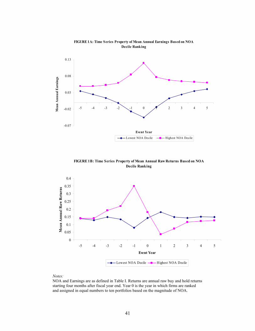
FIGURE 1A: Time Series Property of Mean Annual Earnings Based on NOA Decile Ranking
-0.07
-0.02
0.03
0.08
0.13
-5 -4 -3 -2 -1 0 1 2 3 4 5
Event Year
Mea
n A
nnua
l Ear
ning
s
Lowest NOA Decile Highest NOA Decile
FIGURE 1B: Time Series Property of Mean Annual Raw Returns Based on NOA Decile Ranking
0
0.05
0.1
0.15
0.2
0.25
0.3
0.35
0.4
-5 -4 -3 -2 -1 0 1 2 3 4 5
Event Year
Mea
n A
nnua
l Raw
Ret
urns
Lowest NOA Decile Highest NOA Decile
Notes: NOA and Earnings are as defined in Table I. Returns are annual raw buy and hold returns starting four months after fiscal year end. Year 0 is the year in which firms are ranked and assigned in equal numbers to ten portfolios based on the magnitude of NOA.
41
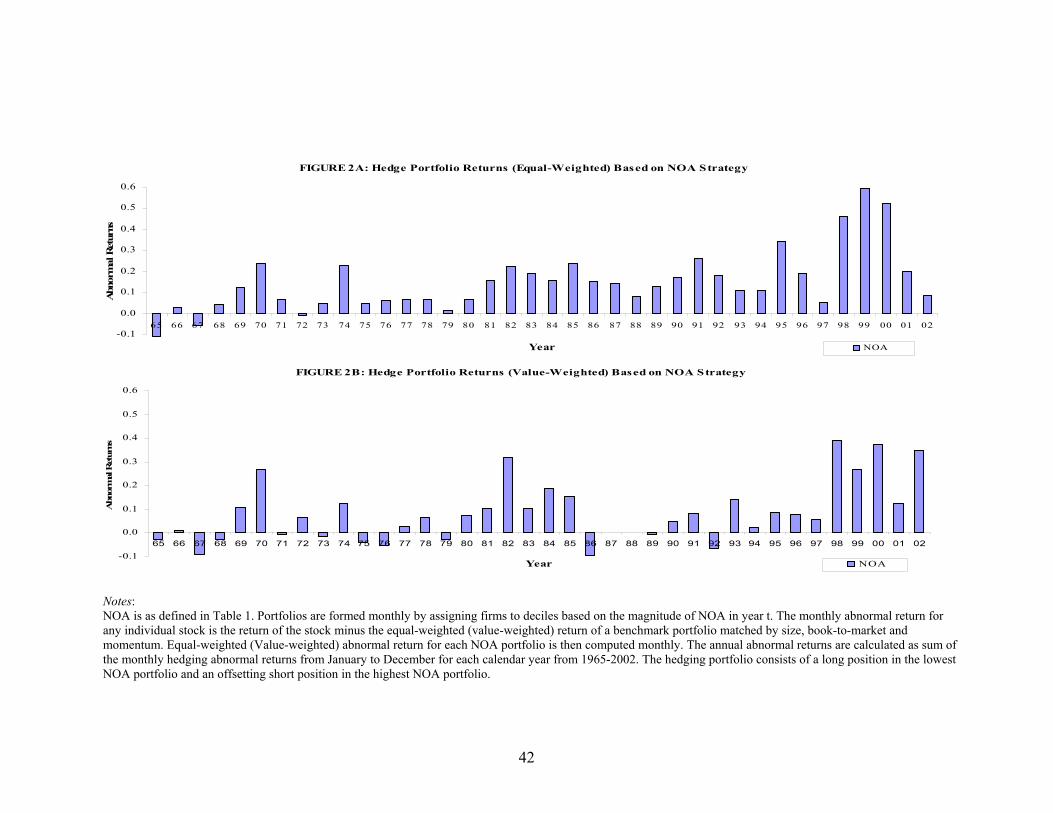
FIGURE 2A: Hedge Portfolio Returns (Equal-Weighted) Based on NOA Strategy
-0.1
0.0
0.1
0.2
0.3
0.4
0.5
0.6
65 66 67 68 69 70 71 72 73 74 75 76 77 78 79 80 81 82 83 84 85 86 87 88 89 90 91 92 93 94 95 96 97 98 99 00 01 02
Year
Abn
orm
al R
etur
ns
NOA FIGURE 2B: Hedge Portfolio Returns (Value-Weighted) Based on NOA Strategy
-0.1
0.0
0.1
0.2
0.3
0.4
0.5
0.6
65 66 67 68 69 70 71 72 73 74 75 76 77 78 79 80 81 82 83 84 85 86 87 88 89 90 91 92 93 94 95 96 97 98 99 00 01 02
Year
Abn
orm
al R
etur
ns
NOA
Notes: NOA is as defined in Table 1. Portfolios are formed monthly by assigning firms to deciles based on the magnitude of NOA in year t. The monthly abnormal return for any individual stock is the return of the stock minus the equal-weighted (value-weighted) return of a benchmark portfolio matched by size, book-to-market and momentum. Equal-weighted (Value-weighted) abnormal return for each NOA portfolio is then computed monthly. The annual abnormal returns are calculated as sum of the monthly hedging abnormal returns from January to December for each calendar year from 1965-2002. The hedging portfolio consists of a long position in the lowest NOA portfolio and an offsetting short position in the highest NOA portfolio.
42
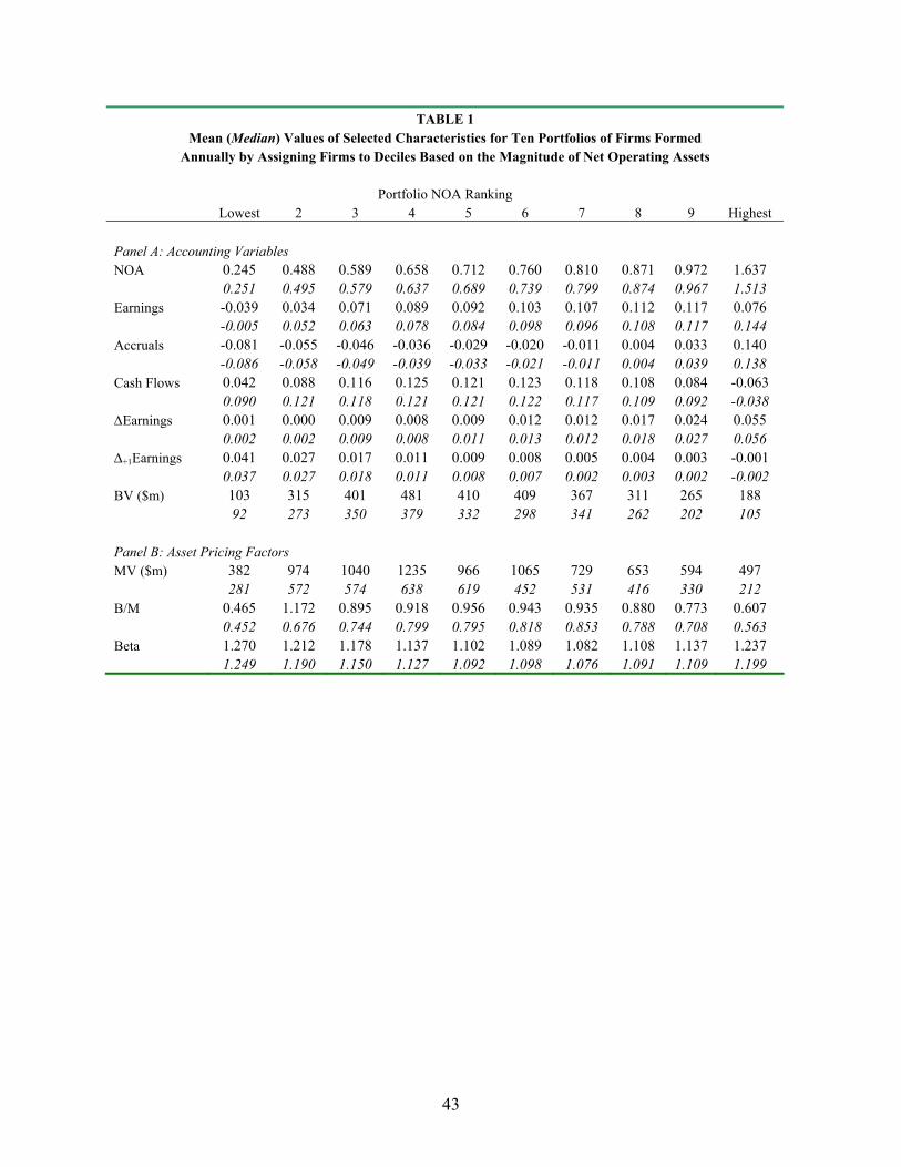
TABLE 1 Mean (Median) Values of Selected Characteristics for Ten Portfolios of Firms Formed
Annually by Assigning Firms to Deciles Based on the Magnitude of Net Operating Assets
Portfolio NOA Ranking Lowest 2 3 4 5 6 7 8 9 Highest Panel A: Accounting Variables NOA 0.245 0.488 0.589 0.658 0.712 0.760 0.810 0.871 0.972 1.637 0.251 0.495 0.579 0.637 0.689 0.739 0.799 0.874 0.967 1.513 Earnings -0.039 0.034 0.071 0.089 0.092 0.103 0.107 0.112 0.117 0.076 -0.005 0.052 0.063 0.078 0.084 0.098 0.096 0.108 0.117 0.144 Accruals -0.081 -0.055 -0.046 -0.036 -0.029 -0.020 -0.011 0.004 0.033 0.140 -0.086 -0.058 -0.049 -0.039 -0.033 -0.021 -0.011 0.004 0.039 0.138 Cash Flows 0.042 0.088 0.116 0.125 0.121 0.123 0.118 0.108 0.084 -0.063 0.090 0.121 0.118 0.121 0.121 0.122 0.117 0.109 0.092 -0.038 ∆Earnings 0.001 0.000 0.009 0.008 0.009 0.012 0.012 0.017 0.024 0.055 0.002 0.002 0.009 0.008 0.011 0.013 0.012 0.018 0.027 0.056 ∆+1Earnings 0.041 0.027 0.017 0.011 0.009 0.008 0.005 0.004 0.003 -0.001 0.037 0.027 0.018 0.011 0.008 0.007 0.002 0.003 0.002 -0.002 BV ($m) 103 315 401 481 410 409 367 311 265 188 92 273 350 379 332 298 341 262 202 105 Panel B: Asset Pricing Factors MV ($m) 382 974 1040 1235 966 1065 729 653 594 497 281 572 574 638 619 452 531 416 330 212 B/M 0.465 1.172 0.895 0.918 0.956 0.943 0.935 0.880 0.773 0.607 0.452 0.676 0.744 0.799 0.795 0.818 0.853 0.788 0.708 0.563 Beta 1.270 1.212 1.178 1.137 1.102 1.089 1.082 1.108 1.137 1.237 1.249 1.190 1.150 1.127 1.092 1.098 1.076 1.091 1.109 1.199
43

Notes: The sample consists of a maximum of approximately 1.63 million firm-month observations covering NYSE, AMEX and Nasdaq firms with available data from July 1964 to December 2002, and a total of 141,254 firm-year observations from fiscal year 1963 to 2000. Monthly returns are analyzed using the characteristic-matched portfolio benchmark and Fama-Macbeth-like cross-sectional regressions; annual returns are used in the Mishkin test for market efficiency. Variable Measurement Raw NOA = Operating Assets (OA)-Operating Liabilities (OL), where (Compustat item numbers in parentheses) OA = Total Assets (Compustat #6) – Cash and Short Term Investment (Compustat #1) OL = Total Assets – STD – LTD – MI – PS - CE
STD = Debt included in current liabilities (Compustat #34) LTD = Long Term Debt (Compustat #9) MI = Minority Interests (Compustat #38) PS = Preferred Stocks (Compustat #130) CE = Common Equity (Compustat #60) NOA, net operating assets = Raw NOA /Lagged Total Assets Earnings = Income From Continuing Operations (Compustat#178)/lagged total assets Raw Accruals = (∆CA-∆Cash)-(∆CL-∆STD-∆TP)-Dep, where ∆ is the annual change, and
CA = Current Assets (Compustat #4) CL = Current Liabilities (Compustat #5) TP = Income Tax Payable (Compustat #71) Dep = Depreciation and Amortization (Compustat #14) Accruals = Raw Accruals / Lagged Total Assets Cash Flows = Earnings - Accruals (as defined above) ∆Earnings = Current Change in Earnings (Earningst-Earningst-1) ∆t+1Earnings = Future Change in Earnings (Earningst+1-Earningst) MV = Fiscal Year End Closing Price*Shares Outstanding (Compustat #199*#25) BV = Book Value of Common Equity (Compustat #60), measured at fiscal year end B/M = BV / MV (as defined above) Beta = Estimated from a regression of monthly raw returns on the CRSP NYSE/AMEX
equal weighted monthly return index. The regression is estimated using the 60-month return period ending four months after each firm’s fiscal year end.
44
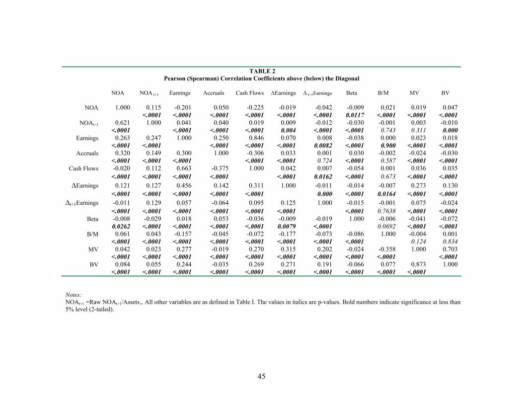
TABLE 2
Pearson (Spearman) Correlation Coefficients above (below) the Diagonal
NOA NOA t+1 Earnings Accruals Cash Flows
∆Earnings
∆ t+1Earnings
Beta B/M MV BV
NOA 1.000 0.115 -0.201 0.050 -0.225 -0.019 -0.042 -0.009 0.021 0.019 0.047 <.0001 <.0001 <.0001 <.0001 <.0001 <.0001 0.0117 <.0001 <.0001 <.0001
NOAt+1 0.621 1.000
0.041 0.040 0.019 0.009 -0.012 -0.030 -0.001 0.003 -0.010 <.0001 <.0001 <.0001 <.0001 0.004 <.0001 <.0001 0.743 0.311 0.000
Earnings 0.263 0.247 1.000 0.250 0.846 0.070 0.008 -0.038 0.000 0.023 0.018 <.0001 <.0001 <.0001 <.0001 <.0001 0.0082 <.0001 0.900 <.0001 <.0001
Accruals 0.320 0.149 0.300 1.000 -0.306 0.033 0.001 0.030 -0.002 -0.024 -0.030 <.0001 <.0001 <.0001 <.0001 <.0001 0.724 <.0001 0.587 <.0001 <.0001
Cash Flows -0.020 0.112 0.663 -0.375 1.000 0.042 0.007 -0.054 0.001 0.036 0.035 <.0001 <.0001 <.0001 <.0001 <.0001 0.0162 <.0001 0.673 <.0001 <.0001
∆Earnings 0.121 0.127 0.456 0.142 0.311 1.000 -0.011 -0.014 -0.007 0.273 0.130 <.0001 <.0001 <.0001 <.0001 <.0001 0.000 <.0001 0.0164 <.0001 <.0001
∆t+1Earnings -0.011 0.129 0.057 -0.064 0.095 0.125 1.000 -0.015 -0.001 0.075 -0.024 <.0001 <.0001 <.0001 <.0001 <.0001 <.0001 <.0001 0.7638 <.0001 <.0001
Beta -0.008 -0.029 0.018 0.053 -0.036 -0.009 -0.019 1.000 -0.006 -0.041 -0.072 0.0262 <.0001 <.0001 <.0001 <.0001 0.0079 <.0001 0.0692 <.0001 <.0001
B/M 0.061 0.043 -0.157 -0.045 -0.072 -0.177 -0.073 -0.086 1.000 -0.004 0.001 <.0001 <.0001 <.0001 <.0001 <.0001 <.0001 <.0001 <.0001 0.124 0.834
MV 0.042 0.023 0.277 -0.019 0.270 0.315 0.202 -0.024 -0.358 1.000 0.703 <.0001 <.0001 <.0001 <.0001 <.0001 <.0001 <.0001 <.0001 <.0001 <.0001
BV 0.084 0.055 0.244 -0.035 0.269 0.271 0.191 -0.066 0.077 0.873 1.000 <.0001 <.0001 <.0001 <.0001 <.0001 <.0001 <.0001 <.0001 <.0001 <.0001
Notes: NOAt+1 =Raw NOAt+1/Assets t. All other variables are as defined in Table I. The values in italics are p-values. Bold numbers indicate significance at less than 5% level (2-tailed).
45
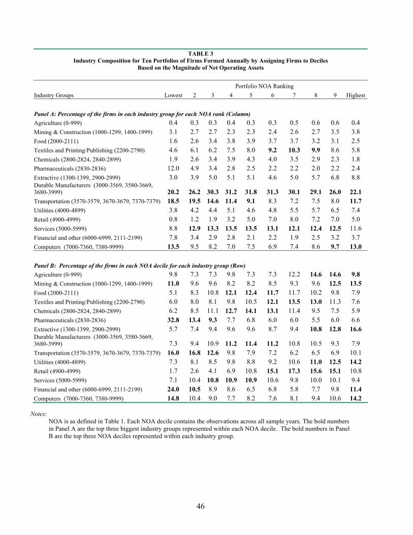
TABLE 3 Industry Composition for Ten Portfolios of Firms Formed Annually by Assigning Firms to Deciles
Based on the Magnitude of Net Operating Assets Portfolio NOA Ranking Industry Groups Lowest 2 3 4 5 6 7 8 9 Highest Panel A: Percentage of the firms in each industry group for each NOA rank (Column) Agriculture (0-999) 0.4 0.3 0.3 0.4 0.3 0.3 0.5 0.6 0.6 0.4 Mining & Construction (1000-1299, 1400-1999) 3.1 2.7 2.7 2.3 2.3 2.4 2.6 2.7 3.5 3.8 Food (2000-2111) 1.6 2.6 3.4 3.8 3.9 3.7 3.7 3.2 3.1 2.5 Textiles and Printing/Publishing (2200-2790) 4.6 6.1 6.2 7.5 8.0 9.2 10.3 9.9 8.6 5.8 Chemicals (2800-2824, 2840-2899) 1.9 2.6 3.4 3.9 4.3 4.0 3.5 2.9 2.3 1.8 Pharmaceuticals (2830-2836) 12.0 4.9 3.4 2.8 2.5 2.2 2.2 2.0 2.2 2.4 Extractive (1300-1399, 2900-2999) 3.0 3.9 5.0 5.1 5.1 4.6 5.0 5.7 6.8 8.8 Durable Manufacturers (3000-3569, 3580-3669, 3680-3999) 20.2 26.2 30.3 31.2 31.8 31.3 30.1 29.1 26.0 22.1 Transportation (3570-3579, 3670-3679, 7370-7379) 18.5 19.5 14.6 11.4 9.1 8.3 7.2 7.5 8.0 11.7 Utilities (4000-4899) 3.8 4.2 4.4 5.1 4.6 4.8 5.5 5.7 6.5 7.4 Retail (4900-4999) 0.8 1.2 1.9 3.2 5.0 7.0 8.0 7.2 7.0 5.0 Services (5000-5999) 8.8 12.9 13.3 13.5 13.5 13.1 12.1 12.4 12.5 11.6 Financial and other (6000-6999, 2111-2199) 7.8 3.4 2.9 2.8 2.1 2.2 1.9 2.5 3.2 3.7 Computers (7000-7360, 7380-9999) 13.5 9.5 8.2 7.0 7.5 6.9 7.4 8.6 9.7 13.0 Panel B: Percentage of the firms in each NOA decile for each industry group (Row) Agriculture (0-999) 9.8 7.3 7.3 9.8 7.3 7.3 12.2 14.6 14.6 9.8 Mining & Construction (1000-1299, 1400-1999) 11.0 9.6 9.6 8.2 8.2 8.5 9.3 9.6 12.5 13.5 Food (2000-2111) 5.1 8.3 10.8 12.1 12.4 11.7 11.7 10.2 9.8 7.9 Textiles and Printing/Publishing (2200-2790) 6.0 8.0 8.1 9.8 10.5 12.1 13.5 13.0 11.3 7.6 Chemicals (2800-2824, 2840-2899) 6.2 8.5 11.1 12.7 14.1 13.1 11.4 9.5 7.5 5.9 Pharmaceuticals (2830-2836) 32.8 13.4 9.3 7.7 6.8 6.0 6.0 5.5 6.0 6.6 Extractive (1300-1399, 2900-2999) 5.7 7.4 9.4 9.6 9.6 8.7 9.4 10.8 12.8 16.6 Durable Manufacturers (3000-3569, 3580-3669, 3680-3999) 7.3 9.4 10.9 11.2 11.4 11.2 10.8 10.5 9.3 7.9 Transportation (3570-3579, 3670-3679, 7370-7379) 16.0 16.8 12.6 9.8 7.9 7.2 6.2 6.5 6.9 10.1 Utilities (4000-4899) 7.3 8.1 8.5 9.8 8.8 9.2 10.6 11.0 12.5 14.2 Retail (4900-4999) 1.7 2.6 4.1 6.9 10.8 15.1 17.3 15.6 15.1 10.8 Services (5000-5999) 7.1 10.4 10.8 10.9 10.9 10.6 9.8 10.0 10.1 9.4 Financial and other (6000-6999, 2111-2199) 24.0 10.5 8.9 8.6 6.5 6.8 5.8 7.7 9.8 11.4 Computers (7000-7360, 7380-9999) 14.8 10.4 9.0 7.7 8.2 7.6 8.1 9.4 10.6 14.2
Notes:
NOA is as defined in Table 1. Each NOA decile contains the observations across all sample years. The bold numbers in Panel A are the top three biggest industry groups represented within each NOA decile. The bold numbers in Panel B are the top three NOA deciles represented within each industry group.
46
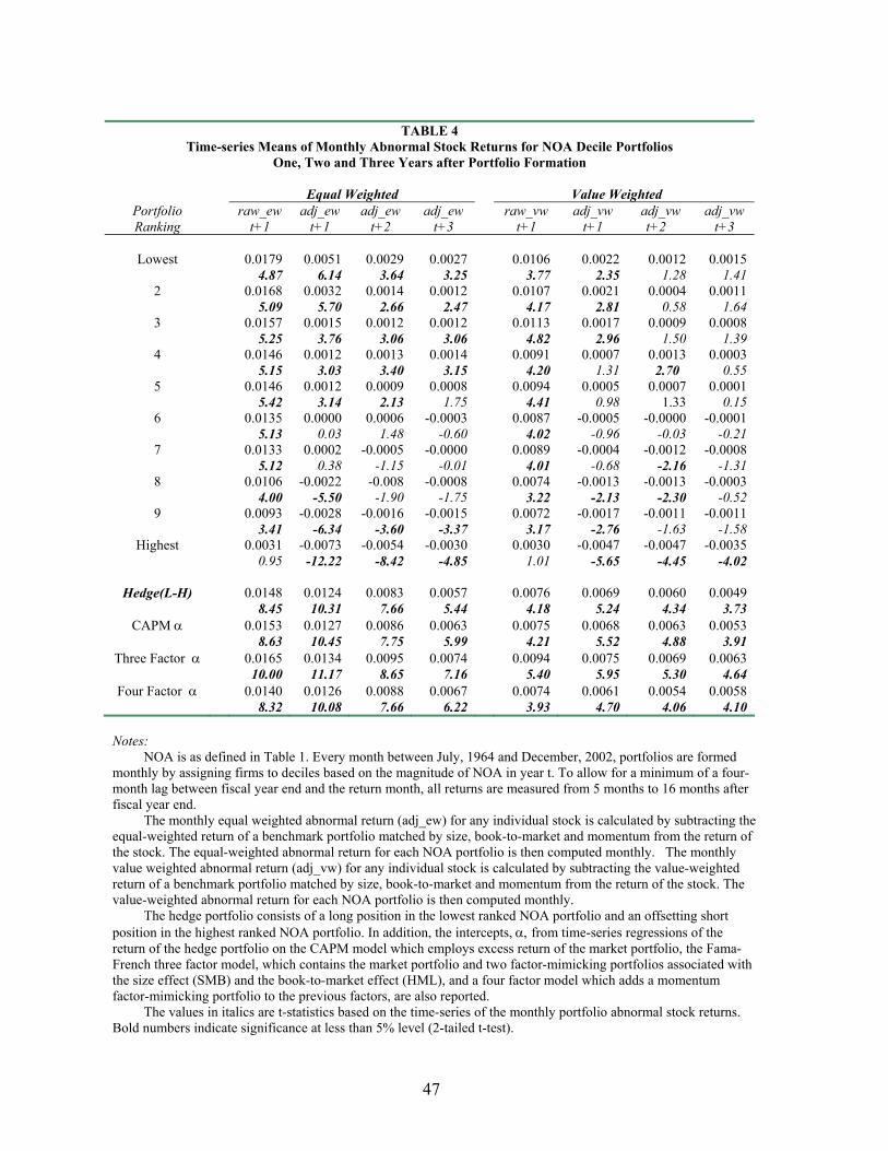
TABLE 4
Time-series Means of Monthly Abnormal Stock Returns for NOA Decile Portfolios One, Two and Three Years after Portfolio Formation
Equal Weighted Value Weighted
Portfolio raw_ew adj_ew adj_ew adj_ew raw_vw adj_vw adj_vw adj_vw Ranking t+1 t+1 t+2 t+3 t+1 t+1 t+2 t+3
Lowest 0.0179 0.0051 0.0029 0.0027 0.0106 0.0022 0.0012 0.0015
4.87 6.14 3.64 3.25 3.77 2.35 1.28 1.41 2 0.0168 0.0032 0.0014 0.0012 0.0107 0.0021 0.0004 0.0011 5.09 5.70 2.66 2.47 4.17 2.81 0.58 1.64 3 0.0157 0.0015 0.0012 0.0012 0.0113 0.0017 0.0009 0.0008 5.25 3.76 3.06 3.06 4.82 2.96 1.50 1.39 4 0.0146 0.0012 0.0013 0.0014 0.0091 0.0007 0.0013 0.0003 5.15 3.03 3.40 3.15 4.20 1.31 2.70 0.55 5 0.0146 0.0012 0.0009 0.0008 0.0094 0.0005 0.0007 0.0001 5.42 3.14 2.13 1.75 4.41 0.98 1.33 0.15 6 0.0135 0.0000 0.0006 -0.0003 0.0087 -0.0005 -0.0000 -0.0001 5.13 0.03 1.48 -0.60 4.02 -0.96 -0.03 -0.21 7 0.0133 0.0002 -0.0005 -0.0000 0.0089 -0.0004 -0.0012 -0.0008 5.12 0.38 -1.15 -0.01 4.01 -0.68 -2.16 -1.31 8 0.0106 -0.0022 -0.008 -0.0008 0.0074 -0.0013 -0.0013 -0.0003 4.00 -5.50 -1.90 -1.75 3.22 -2.13 -2.30 -0.52 9 0.0093 -0.0028 -0.0016 -0.0015 0.0072 -0.0017 -0.0011 -0.0011 3.41 -6.34 -3.60 -3.37 3.17 -2.76 -1.63 -1.58
Highest 0.0031 -0.0073 -0.0054 -0.0030 0.0030 -0.0047 -0.0047 -0.0035 0.95 -12.22 -8.42 -4.85 1.01 -5.65 -4.45 -4.02
Hedge(L-H) 0.0148 0.0124 0.0083 0.0057 0.0076 0.0069 0.0060 0.0049 8.45 10.31 7.66 5.44 4.18 5.24 4.34 3.73
CAPM α 0.0153 0.0127 0.0086 0.0063 0.0075 0.0068 0.0063 0.0053 8.63 10.45 7.75 5.99 4.21 5.52 4.88 3.91
Three Factor α 0.0165 0.0134 0.0095 0.0074 0.0094 0.0075 0.0069 0.0063 10.00 11.17 8.65 7.16 5.40 5.95 5.30 4.64
Four Factor α 0.0140 0.0126 0.0088 0.0067 0.0074 0.0061 0.0054 0.0058 8.32 10.08 7.66 6.22 3.93 4.70 4.06 4.10
Notes: NOA is as defined in Table 1. Every month between July, 1964 and December, 2002, portfolios are formed monthly by assigning firms to deciles based on the magnitude of NOA in year t. To allow for a minimum of a four-month lag between fiscal year end and the return month, all returns are measured from 5 months to 16 months after fiscal year end. The monthly equal weighted abnormal return (adj_ew) for any individual stock is calculated by subtracting the equal-weighted return of a benchmark portfolio matched by size, book-to-market and momentum from the return of the stock. The equal-weighted abnormal return for each NOA portfolio is then computed monthly. The monthly value weighted abnormal return (adj_vw) for any individual stock is calculated by subtracting the value-weighted return of a benchmark portfolio matched by size, book-to-market and momentum from the return of the stock. The value-weighted abnormal return for each NOA portfolio is then computed monthly. The hedge portfolio consists of a long position in the lowest ranked NOA portfolio and an offsetting short position in the highest ranked NOA portfolio. In addition, the intercepts, α, from time-series regressions of the return of the hedge portfolio on the CAPM model which employs excess return of the market portfolio, the Fama-French three factor model, which contains the market portfolio and two factor-mimicking portfolios associated with the size effect (SMB) and the book-to-market effect (HML), and a four factor model which adds a momentum factor-mimicking portfolio to the previous factors, are also reported. The values in italics are t-statistics based on the time-series of the monthly portfolio abnormal stock returns. Bold numbers indicate significance at less than 5% level (2-tailed t-test).
47
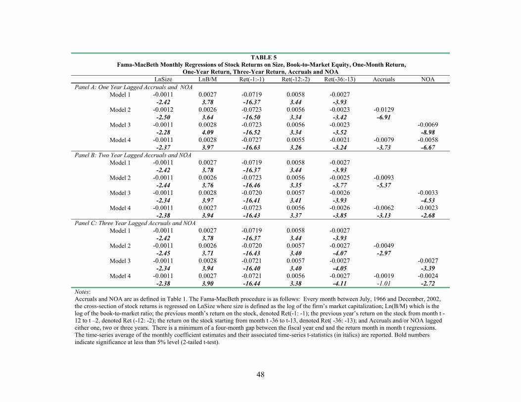
TABLE 5 Fama-MacBeth Monthly Regressions of Stock Returns on Size, Book-to-Market Equity, One-Month Return,
One-Year Return, Three-Year Return, Accruals and NOA LnSize LnB/M Ret(-1:-1) Ret(-12:-2) Ret(-36:-13) Accruals NOA Panel A: One Year Lagged Accruals and NOA Model 1
-0.0011 0.0027
-0.0719 0.0058 -0.0027-2.42 3.78 -16.37 3.44 -3.93
Model 2
-0.0012 0.0026 -0.0723 0.0056 -0.0023 -0.0129-2.50 3.64 -16.50 3.34 -3.42 -6.91
Model 3
-0.0011 0.0028 -0.0723 0.0056 -0.0023 -0.0069-2.28 4.09 -16.52 3.34 -3.52 -8.98
Model 4
-0.0011 0.0028 -0.0727 0.0055 -0.0021 -0.0079 -0.0058-2.37 3.97 -16.63 3.26 -3.24 -3.73 -6.67
Panel B: Two Year Lagged Accruals and NOA Model 1
-0.0011 0.0027
-0.0719 0.0058 -0.0027-2.42 3.78 -16.37 3.44 -3.93
Model 2
-0.0011 0.0026 -0.0723 0.0056 -0.0025 -0.0093-2.44 3.76 -16.46 3.35 -3.77 -5.37
Model 3
-0.0011 0.0028 -0.0720 0.0057 -0.0026 -0.0033-2.34 3.97 -16.41 3.41 -3.93 -4.53
Model 4
-0.0011 0.0027 -0.0723 0.0056 -0.0026 -0.0062 -0.0023-2.38 3.94 -16.43 3.37 -3.85 -3.13 -2.68
Panel C: Three Year Lagged Accruals and NOA Model 1
-0.0011 0.0027
-0.0719 0.0058 -0.0027-2.42 3.78 -16.37 3.44 -3.93
Model 2
-0.0011 0.0026 -0.0720 0.0057 -0.0027 -0.0049-2.45 3.71 -16.43 3.40 -4.07 -2.97
Model 3
-0.0011 0.0028 -0.0721 0.0057 -0.0027 -0.0027-2.34 3.94 -16.40 3.40 -4.05 -3.39
Model 4 -0.0011 0.0027 -0.0721 0.0056 -0.0027 -0.0019 -0.0024 -2.38 3.90 -16.44 3.38 -4.11 -1.01 -2.72 Notes: Accruals and NOA are as defined in Table 1. The Fama-MacBeth procedure is as follows: Every month between July, 1966 and December, 2002, the cross-section of stock returns is regressed on LnSize where size is defined as the log of the firm’s market capitalization; Ln(B/M) which is the log of the book-to-market ratio; the previous month’s return on the stock, denoted Ret(-1: -1); the previous year’s return on the stock from month t -12 to t –2, denoted Ret (-12: -2); the return on the stock starting from month t -36 to t-13, denoted Ret( -36: -13); and Accruals and/or NOA lagged either one, two or three years. There is a minimum of a four-month gap between the fiscal year end and the return month in month t regressions. The time-series average of the monthly coefficient estimates and their associated time-series t-statistics (in italics) are reported. Bold numbers indicate significance at less than 5% level (2-tailed t-test).
48
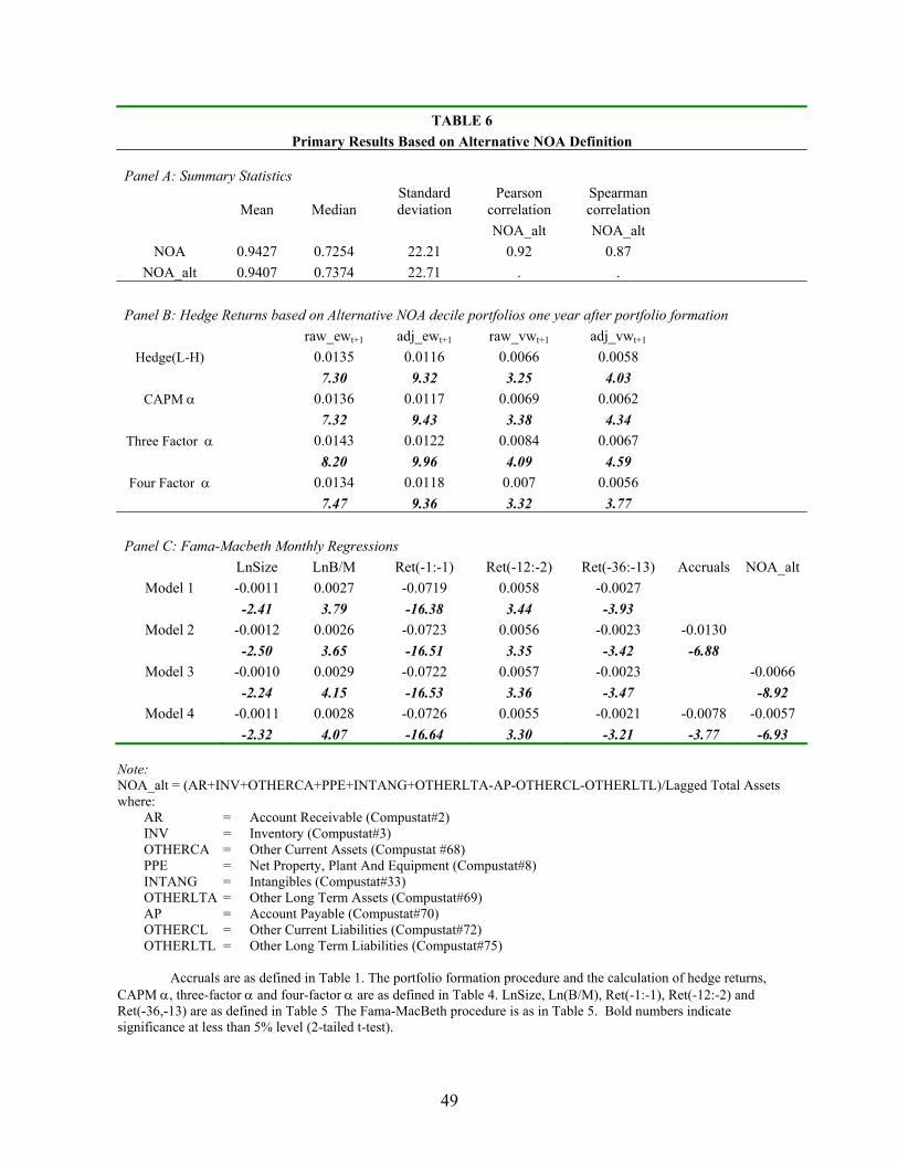
TABLE 6 Primary Results Based on Alternative NOA Definition
Panel A: Summary Statistics
Mean Median Standard deviation
Pearson correlation
Spearman correlation
NOA_alt NOA_alt NOA 0.9427 0.7254 22.21 0.92 0.87
NOA_alt 0.9407 0.7374 22.71 . .
Panel B: Hedge Returns based on Alternative NOA decile portfolios one year after portfolio formation raw_ewt+1 adj_ewt+1 raw_vwt+1 adj_vwt+1
Hedge(L-H) 0.0135 0.0116 0.0066 0.0058 7.30 9.32 3.25 4.03
CAPM α 0.0136 0.0117 0.0069 0.0062 7.32 9.43 3.38 4.34
Three Factor α 0.0143 0.0122 0.0084 0.0067 8.20 9.96 4.09 4.59
Four Factor α 0.0134 0.0118 0.007 0.0056 7.47 9.36 3.32 3.77
Panel C: Fama-Macbeth Monthly Regressions LnSize LnB/M Ret(-1:-1) Ret(-12:-2) Ret(-36:-13) Accruals NOA_alt
Model 1 -0.0011 0.0027 -0.0719 0.0058 -0.0027 -2.41 3.79 -16.38 3.44 -3.93
Model 2 -0.0012 0.0026 -0.0723 0.0056 -0.0023 -0.0130 -2.50 3.65 -16.51 3.35 -3.42 -6.88
Model 3 -0.0010 0.0029 -0.0722 0.0057 -0.0023 -0.0066 -2.24 4.15 -16.53 3.36 -3.47 -8.92
Model 4 -0.0011 0.0028 -0.0726 0.0055 -0.0021 -0.0078 -0.0057 -2.32 4.07 -16.64 3.30 -3.21 -3.77 -6.93
Note: NOA_alt = (AR+INV+OTHERCA+PPE+INTANG+OTHERLTA-AP-OTHERCL-OTHERLTL)/Lagged Total Assets where:
AR = Account Receivable (Compustat#2) INV = Inventory (Compustat#3) OTHERCA = Other Current Assets (Compustat #68) PPE = Net Property, Plant And Equipment (Compustat#8) INTANG = Intangibles (Compustat#33) OTHERLTA = Other Long Term Assets (Compustat#69) AP = Account Payable (Compustat#70) OTHERCL = Other Current Liabilities (Compustat#72) OTHERLTL = Other Long Term Liabilities (Compustat#75)
Accruals are as defined in Table 1. The portfolio formation procedure and the calculation of hedge returns,
CAPM α, three-factor α and four-factor α are as defined in Table 4. LnSize, Ln(B/M), Ret(-1:-1), Ret(-12:-2) and Ret(-36,-13) are as defined in Table 5 The Fama-MacBeth procedure is as in Table 5. Bold numbers indicate significance at less than 5% level (2-tailed t-test).
49
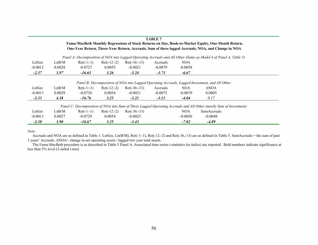
TABLE 7 Fama-MacBeth Monthly Regressions of Stock Returns on Size, Book-to-Market Equity, One-Month Return, One-Year Return, Three-Year Return, Accruals, Sum of three lagged Accruals, NOA, and Change in NOA
Panel A: Decomposition of NOA into Lagged Operating Accruals and All Other (Same as Model 4 of Panel A, Table 5)
LnSize
LnB/M Ret(-1:-1) Ret(-12:-2) Ret(-36:-13) Accruals NOA-0.0011 0.0028 -0.0727 0.0055 -0.0021 -0.0079 -0.0058
-2.37 3.97 -16.63 3.26 -3.24 -3.73 -6.67
Panel B: Decomposition of NOA into Lagged Operating Accruals, Lagged Investment, and All Other LnSize
LnB/M Ret(-1:-1) Ret(-12:-2) Ret(-36:-13)
Accruals NOA ∆NOA -0.0011 0.0029 -0.0728 0.0054 -0.0021 -0.0072 -0.0070 0.0003
-2.33 4.38 -16.76 3.25 -3.21 -3.11 -4.04 0.17
Panel C: Decomposition of NOA into Sum of Three Lagged Operating Accruals and All Other (mostly Sum of Investment) LnSize
LnB/M Ret(-1:-1) Ret(-12:-2) Ret(-36:-13) NOA SumAccruals -0.0011 0.0027 -0.0729 0.0054 -0.0023 -0.0056 -0.0048
-2.38 3.90 -16.67 3.25 -3.43 -7.02 -4.89 Note: Accruals and NOA are as defined in Table 1. LnSize, Ln(B/M), Ret(-1:-1), Ret(-12:-2) and Ret(-36,-13) are as defined in Table 5. SumAccruals = the sum of past 3 years’ Accruals. ∆NOA= change in net operating assets / lagged two year total assets. The Fama-MacBeth procedure is as described in Table 5 Panel A. Associated time-series t-statistics (in italics) are reported. Bold numbers indicate significance at less than 5% level (2-tailed t-test).
50
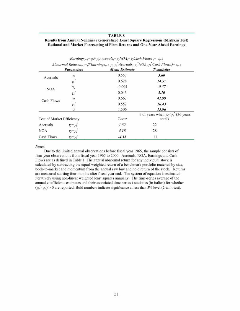
TABLE 8
Results from Annual Nonlinear Generalized Least Square Regressions (Mishkin Test) Rational and Market Forecasting of Firm Returns and One-Year Ahead Earnings
Earningst+1=γ0+γ1Accrualst+γ2NOAt+γ3Cash Flows t+ vt+1 Abnormal Returnst+1=β(Earningst+1-γ0-γ1
*Accrualst-γ2*NOAt-γ3
*Cash Flowst)+εt+1 Parameters Mean Estimate T-statistics
γ1 0.557 3.60 Accruals γ1
∗ 0.628 14.57 γ2 -0.004 -0.57 NOA γ2
∗ 0.043 3.10 γ3 0.663 41.99 Cash Flows γ3
∗ 0.552 16.43 β 1.506 13.96
Test of Market Efficiency: T-test # of years when γn<γn
* (36 years total)
Accruals
γ1=γ1* 1.82 22
NOA γ2=γ2* 4.18 28
Cash Flows γ3=γ3* -4.18 11
Notes: Due to the limited annual observations before fiscal year 1965, the sample consists of firm-year observations from fiscal year 1965 to 2000. Accruals, NOA, Earnings and Cash Flows are as defined in Table 1. The annual abnormal return for any individual stock is calculated by subtracting the equal-weighted return of a benchmark portfolio matched by size, book-to-market and momentum from the annual raw buy and hold return of the stock. Returns are measured starting four months after fiscal year end. The system of equation is estimated iteratively using non-linear weighted least squares annually. The time-series average of the annual coefficients estimates and their associated time-series t-statistics (in italics) for whether (γn
*- γn ) > 0 are reported. Bold numbers indicate significance at less than 5% level (2-tail t-test).
51