do patients choose hospitals - york.ac.uk · pdf filedo patients choose hospitals that improve...
TRANSCRIPT

CHE Research Paper 111
Do Patients Choose Hospitals That Improve Their Health?
Nils Gutacker, Luigi Siciliani, Giuseppe Moscelli, Hugh Gravelle


Do patients choose hospitals that improve their health?
1Nils Gutacker 2Luigi Siciliani 1Giuseppe Moscelli 1Hugh Gravelle
1Centre for Health Economics, University of York, UK 2Department of Economics and Related Studies, University of York, UK May 2015

Background to series
CHE Discussion Papers (DPs) began publication in 1983 as a means of making current research material more widely available to health economists and other potential users. So as to speed up the dissemination process, papers were originally published by CHE and distributed by post to a worldwide readership.
The CHE Research Paper series takes over that function and provides access to current research output via web-based publication, although hard copy will continue to be available (but subject to charge).
Acknowledgements
We are grateful for comments and suggestions from Alistair McGuire, Andrew Street, Karen Bloor, Richard Cookson and those received during presentations at the Universities of Birmingham, Newcastle, York and Melbourne, the King's Fund, and the Leeds meeting of the Health Economic Study Group. This research was funded by the Department of Health in England under the Policy Research Unit in the Economics of Health and Social Care Systems (Ref 103/0001). The views expressed are those of the authors and not necessarily those of the funders. Hospital Episode Statistics are copyright 2015, re-used with the permission of The Health & Social Care Information Centre. All rights reserved.
Disclaimer
Papers published in the CHE Research Paper (RP) series are intended as a contribution to current research. Work and ideas reported in RPs may not always represent the final position and as such may sometimes need to be treated as work in progress. The material and views expressed in RPs are solely those of the authors and should not be interpreted as representing the collective views of CHE research staff or their research funders.
Further copies
Copies of this paper are freely available to download from the CHE website www.york.ac.uk/che/publications/ Access to downloaded material is provided on the understanding that it is intended for personal use. Copies of downloaded papers may be distributed to third-parties subject to the proviso that the CHE publication source is properly acknowledged and that such distribution is not subject to any payment.
Printed copies are available on request at a charge of £5.00 per copy. Please contact the CHE Publications Office, email [email protected], telephone 01904 321405 for further details.
Centre for Health Economics Alcuin College University of York York, UK www.york.ac.uk/che
© Nils Gutacker, Luigi Siciliani, Giuseppe Moscelli, Hugh Gravelle

Do patients choose hospitals that improve their health? i
Abstract
Many health care systems collect and disseminate information on provider quality in order to facilitatepatient choice and induce competitive behaviour amongst providers. The Department of Health inEngland has recently mandated the collection of patient-reported health outcome measures (PROMs)for the purpose of performance assessment and consumer information. This is the first attempt toroutinely measure the gain in health that patients experience as the result of care and thus offer a morecomprehensive picture of hospital quality than existing ‘failure measures’ such as mortality or readmissionrates. In this paper we test whether hospital demand responds to hospital quality measures based onhealth gains in addition to more conventional measures. We estimate hospital choice models for electivehip replacement surgery using rich administrative data for all publicly-funded patients in the English NHSin 2010-2012. Our focus is on two key aspects of hospital choice: 1) the extent to which patients aremore likely to choose hospitals which are expected to achieve larger improvements in patients’ healthand 2) whether patients’ response to quality differs with their morbidity, as measured by pre-operativehealth status, and other characteristics such as age or income deprivation. In order to address potentialendogeneity bias we implement an empirical strategy based on lagged explanatory variables, hospitalfixed effects and a control group design based on demand for emergency hip replacement. Our resultssuggest that hospitals can increase demand by 9% if they increase the average health gains that patientsexperience by one standard deviation. Hospital demand has a higher elasticity with respect to averagehealth gains than emergency readmission or mortality rates. Elective patients are twice as willing asemergency hip replacement patients to travel further for an increase in quality.
Keywords: Patient choice, hospital demand, demand elasticity, quality of care, health outcomes

CHE Research Paper 111 ii

Do patients choose hospitals that improve their health? 1
1. Introduction
Many European healthcare systems have recently extended patients’ right to choose their provider ofelective hospital care (Vrangbaek et al. 2012). Enhanced choice can accommodate patients’ preferencesfor provider characteristics (e.g. proximity, quality or availability of amenities) and create market conditionsthat incentivise providers to compete (Besley and Ghatak 2003). Patients in the English National HealthService (NHS) have to be referred to inpatient services by their general practitioner, who acts as agatekeeper, but are free to choose their preferred provider of care. Prices for hospital care are setnationally and patients do not bear the cost of treatment, so providers are expected to compete forelective patients on the basis of quality. Two prerequisites for such quality competition are that patientsand their agents1 have access to reliable, meaningful and understandable information about the qualityof care offered by alternative providers, and that they act upon such information (Besley and Ghatak2003; Marshall et al. 2004; Faber et al. 2009).
English patients can access comparative information on hospital quality through several channels,including the NHS Choices website, the Health & Social Care Information Centre (HSCIC) websiteand the Dr Foster Hospital Guide. These present information on risk-adjusted 28-day mortality andemergency readmission rates, calculated from routine hospital discharge data. Such indicators havebeen criticised as being incomplete and noisy measures of quality, revealing little about the changes inhealth that the vast majority of patients will experience as the result of treatment (Appleby and Devlin2004; Lilford and Pronovost 2010). This is especially so for mortality rates for common elective operationssuch as hip (0.3%) and knee replacement (0.2%), which are generally very low (Berstock et al. 2014;Belmont et al. 2014).
New hospital quality measures that address these concerns are increasingly available. Since April2009, all providers in the English NHS have been required to collect patient-reported outcome measures(PROMs) for all NHS-funded patients undergoing unilateral hip and knee replacement, varicose veinsurgery or groin hernia repair (Department of Health 2008). PROMs are validated questionnaires usedto elicit patients’ health status and health-related quality of life (HRQoL)2. Each eligible patient is invitedto complete a PROM questionnaire before and three or six months after their surgery. The changes inscores can be interpreted as the improvement in patients’ health and are used for hospital benchmarking(Nuttall et al. 2015; Gutacker, Bojke et al. 2013).
Hospital quality measures derived from PROMs improve over ‘failure’ measures such as mortality oremergency readmission rates in several ways. First, they capture the entire spectrum of health (Applebyand Devlin 2004; Gutacker, Bojke et al. 2013) and thus allow inferences about improvements in health asa consequence of treatment. Second, because post-operative health status is adjusted for pre-operativestatus, it can be argued that they adjust better for case-mix. Finally, PROMs reflect the patients’ viewon their health and health improvement. This, one may argue, makes them especially relevant forprospective patients who are about to choose their provider.
It has been the English Department of Health’s expressed ambition to establish patients’ self-reportedoutcomes as an important component of hospital quality assessment. It was also hoped that such
1 These may include the patient’s general practitioner (GP) as well as family, friends and others. Some patients may not be willing orable to make a choice and their referring GP may choose the most appropriate hospital for them, i.e. the GP acts as an agent tothe patient. It is generally not possible to distinguish between decision makers using administrative data. For simplicity, we willhenceforward denote the decision-maker as the patient.
2 PROMs, such as the EuroQol-5D or the Oxford Hip Score, are widely used in the evaluation of health technologies. The NationalInstitute for Health and Care Excellence (NICE) mandates the use of PROMs for outcome measurement.

CHE Research Paper 111 2
information would be used “by patients and GPs exercising choice” (Department of Health 2008, p.6).Consequently, provider-specific average risk-adjusted changes in health status have been disseminatedonline on a regular basis since the beginning of the national PROM programme (Health & Social CareInformation Centre 2013b). Some patients might access this information directly, whereas others mightrely on their general practitioners, who act as their agent, to retrieve, interpret and communicate thisinformation.
In this paper we test whether hospital demand responds to PROM-based measures of hospital quality inaddition to more conventional measures such as mortality and readmission rates. We estimate a hospitalchoice model for elective hip replacement surgery in the English NHS to identify how hospital choiceresponds to hospital and patient characteristics. Our focus is on two key aspects of hospital choice: 1)whether hospitals with better PROM-derived quality (as measured by the changes in patients’ OxfordHip Score (OHS)) face higher demand and 2) whether patients’ response to quality differs according totheir morbidity, as measured by the pre-operative health status, and other characteristics such as ageor income deprivation. To address potential endogeneity we use lagged quality and waiting times. Wealso undertake robustness checks using hospital fixed effects and by comparing the effects of quality onchoices by elective hip replacement patients with those by emergency hip replacement patients who weexpect to be less sensitive to quality.
This is the first study which explores whether hospital demand responds to quality as measured byaverage patient health gains at provider level, which are derived from patient self-reported outcomemeasures. The existing literature has predominantely focused on failure measures such as mortalityrates, either measured at aggregate hospital level or for specific conditions (e.g Sivey 2008; Beckert et al.2012; Moscone et al. 2012; Gaynor, Propper et al. 2012), readmission rates (Varkevisser et al. 2012;Moscone et al. 2012), as well as hospital reputation and other composite scores (Pope 2009; Varkevisseret al. 2010; Varkevisser et al. 2012; Ruwaard and Douven 2014); see Brekke et al. (2014) for an overview.These studies have typically reported a positive relation between quality and hospital demand. Second,we make novel use of pre-operative individual level PROMs data to explore such questions as whethersicker patients travel farther and choose hospitals with higher quality of care as often assumed in theliterature (Gowrisankaran and Town 1999; Geweke et al. 2003). Previous studies have either relied oninstrumental variable approaches to approximate the role of (unobserved) pre-operative health status ondemand (Gowrisankaran and Town 1999; Geweke et al. 2003) or have used measures of comorbidityburden and past utilisation as proxies for health status. Our data allow us to explore this issue moredirectly. Third, our paper contributes to the small literature on hospital choice in publicly funded healthsystems where demand is rationed by waiting time (Sivey 2012; Beckert et al. 2012; Moscone et al.2012; Gaynor, Propper et al. 2012). Our analysis differs from Beckert et al. (2012), who also studychoice of provider for hip replacement surgery in England, in that we use provider quality measureswhich are procedure-specific and more directly related to the quality of care provided3, explore therole of pre-operative health status, and model the entire relevant market, including private providers ofNHS-funded care.
We find that hospitals with higher PROM scores faces larger demand, and that this effect is unlikely to bedriven entirely by omitted variables. The elasticity of provider demand to average health gains is 1.3 or
3 Beckert et al. (2012) model hospital quality using hospital-wide mortality rates and MRSA infection rates. Aggregate hospitallevel quality indicators, such as the summary hospital mortality indicator (SHMI) used in the English NHS, do not correlate wellwith hip procedure specific outcome measures (Gravelle et al. 2014). In 2010/11, the Pearson correlation coefficients betweenSHMI and the quality measures used in this study were -0.09 (OHS), -0.05 (emergency readmission rate) and 0.10 (mortality rate),respectively.

Do patients choose hospitals that improve their health? 3
about 34 patients for a standard deviation increase in average OHS. A one standard deviation increase inhospital average health gains corresponds to a willingness to travel of just over one additional kilometre.Demand has a higher elasticity with respect to quality measures based on average health gains thanprocedure-specific mortality or readmission rates.
The remainder of the paper is structured as follows: in the next section we describe the data usedin this study in more detail. Section 3 describes our econometric model and sets out our strategy tomitigate potential endogeneity bias. In Section 4 we present the estimated marginal utilities of hospitalcharacteristics and show how these vary with observed patient characteristics. Section 5 presents theestimated effects of changes in providers’ quality on their own demand and that of their competitors.Finally, the last section offers a discussion of the results.
CHE Research Paper 111 4
2. Data
We use patient-level data from Hospital Episode Statistics (HES) for all elective admissions for patientsaged 18 or over who underwent NHS-funded primary (i.e. non-revision) hip replacement surgery4
between April 2010 and March 2013 in NHS or private providers. HES contains rich information onpatients’ demographic and medical characteristics, small area of residence and on the hospital stay.Privately funded patients treated in the private sector are not included in HES and are excluded from ouranalysis5.
We derive four patient variables from HES: patients’ age, gender, the number of emergency admissionsduring the 365 days prior to their hip replacement admission, and the number of Elixhauser comorbidconditions recorded in admissions in the previous year (Elixhauser et al. 1998; Gutacker, Bloor et al.2015). These are available for all patients. We use the 2004 Index of Multiple Deprivation (Noble et al.2006) to attribute to each patient the proportion of residents claiming means-tested benefits in theirLower Super Output Area (LSOA)6, which we interpret as a measure of income deprivation. We measurea patient’s distance from a hospital as the straight-line distance from the centroid of their LSOA7.
The PROM survey invites all NHS-funded hip replacement patients to report their health status andHRQoL before and six months after surgery using a paper-based questionnaire. The pre-operativequestionnaire is administered by the hospital either as part of the admission process or during the lastoutpatient appointment preceding admission. The post-operative questionnaire is administered by acentral agency and posted to the patient. Participation in the PROM survey is compulsory for providersbut optional for patients. Approximately 60% of patients provide complete pre- and postoperative PROMquestionnaires that can be linked to their HES record (Hutchings et al. 2014; Gutacker, Street et al.forthcoming).
Each PROM questionnaire contains three instruments: the Oxford Hip Score (OHS), the EuroQoL-5D(EQ-5D) descriptive system, and the EuroQol Visual Analogue Scale (EQ-VAS). The OHS is a condition-specific instrument that consists of 12 questionnaire items regarding hip-related functioning and pain(Dawson et al. 1996). Each item is scored on a five-point scale, with four indicating no problems andzero indicating severe problems. The overall score is calculated as the sum of all items and rangesfrom zero (worst) to 48 (best). Both EuroQol instruments are generic PROMs, i.e. they can be appliedto different health conditions, and are described in detail elsewhere (Brooks 1996). Previous analysisshowed substantial correlation between the EQ-5D and OHS (Neuburger et al. 2013). Since the OHS is acondition-specific measure and hence plausibly more likely to affect hospital choice for hip replacementswe focus on the OHS throughout this paper.
We use PROMs data in two ways. First, we obtained risk-adjusted hospital-specific PROM changescores for the OHS from the HSCIC website (Health & Social Care Information Centre 2013b). Data are
4 See Department of Health (2008) for procedure codes. We exclude patients that underwent revision surgery to ensure a morehomogeneous sample and because these are believed to be likely to return to the place of initial surgery, independent of observedhospital attributes
5 Approximately 11% of the English population have private (supplementary) insurance and approximately 16% of hip replacementsurgeries are funded privately, either out-of-pocket or through private insurance (Hunt et al. 2013; Commission on the Future ofHealth and Social Care in England 2014)
6 HES records patients’ locations in terms of the LSOA (2001 census boundaries) in which they reside. Each LSOA containsapproximately 1,500 inhabitants and is designed to be homogeneous with respect to tenure and accommodation type.
7 We determine a hospital’s location on the basis of its headquarter’s postcode (for NHS trusts) or the postcode of the individualhospital’s site (for ISTCs). We do not model NHS hospital sites individually as quality information for these providers is onlyrecorded at trust level. This is likely to induce noise to our distance measure.
Do patients choose hospitals that improve their health? 5
reported by financial year, which run from April to March of the next year. The HSCIC excludes from thesereports providers with less than 30 valid pre- and post-operative PROM returns due to concerns aboutstatistical validity and patient anonymity. The case-mix adjustment methodology is reported elsewhere(Department of Health 2012).8 There is some evidence to suggest that the hospital-specific mean scoresare robust to missing data (Gomes et al. forthcoming). Second, in some of our models, we use theinformation in the individual patients’ pre-operative PROMs questionnaires to measure their pre-operativemorbidity and investigate whether choice of provider is affected by pre-operative morbidity. Becausepatients can decline to participate or providers may fail to administer a questionnaire there is scope formissing data and selection bias, and we explore this in the empirical analysis for the subset of modelswhich make use of pre-operative morbidity.
We calculate risk-adjusted hospital-specific 28-day emergency readmission and 28-day mortality ratesafter hip replacement as additional quality measures. These data are presented on patient informationwebsites (such as NHS Choices). To compute them, we link our HES data to Office of National Statisticsdeath records and apply the HSCIC case-mix adjustment as set out in the readmission outcome indicatorspecification (Health & Social Care Information Centre 2013a).9
We group providers into seven categories used by the National Patient Safety Agency: NHS small /medium / large non-teaching trust, NHS teaching trust, NHS specialised orthopaedic provider, NHSmulti-service provider, and NHS Primary Care Trusts (PCTs).10 We also distinguish NHS hospitals fromIndependent Sector Treatment Centres (ISTCs) which are private providers treating NHS patients.
Finally, we derive from HES the median time (in months) that patients in each hospital had to waitbetween the specialist’s decision to add the patient to the waiting list and the admission (the inpatientwait). Patients in the English NHS do not pay for their care directly and waiting times thus serve as arationing mechanism (Iversen and Siciliani 2011). We use the median rather than the mean because itis less affected by a small number of patients with very long wait and thus more representative of theexpected waiting time for a prospective patient. We also conduct sensitivity analysis using the proportionof patients in this hospital that waited longer than 120 days.
8 The adjustment takes into account a range of patient characteristics including age, sex, pre-operative PROM score, socio-economicstatus, comorbidity burden, whether the patient lives alone as well as other indicators of disability.
9 Both readmission and mortality rates are adjusted for age (in 5-yr bands), sex, socio-economic status, comorbidity burden ascaptured by the Charlson index and the number of emergency admissions in the last year.
10 PCTs are responsible for purchasing care for their resident population and, with the exception of the Isle of Wight PCT, do notprovide care themselves.

CHE Research Paper 111 6
3. Methods
3.1. Model specification
We use a random utility choice model (McFadden 1974). Utility of patient i = 1, . . . , N at providerj = 1, . . . , J at time t = 1, . . . , T is Uijt = Vijt + ξjt + εijt, where Vijt depends on observable hospitalcharacteristics and travel distance, ξjt are unobserved hospital characteristics, and εijt is unobservedrandom utility. Patients choose from a set of hospitals Mit ∈ J . Assuming εijt is iid extreme value yieldsthe multinomial logit (MNL) model in which the probability that patient i chooses hospital j is
Pijt = expVijt + ξjt∑
j∈MitVij′ t + ξj′ t
(1)
We assume that all patients who require treatment are treated, i.e. there is no outside option.
In our baseline specification, utility is a linear additive function of the distance from the patient’s residenceto the hospital Dij , distance squared D2
ij , hospital quality metrics Qjt−1, waiting time Wjt−1, and a vectorof time-invariant hospital characteristics Zj , so that
Uijt = D′
ijβd,i +D2′
ijβd2,i +Q′
jt−1βq,i +W′
jt−1βw,i + Z′
jtβz,i + ξjt + εijt (2)
where ξjt and εijt are unobserved. We assume that anticipated utility at a provider is based on itsprevious period’s quality and waiting time because relevant information are available only with a lag(see section 3.2). Varkevisser et al. (2012) make a similar assumption. We also estimate models withcontemporaneous waiting time and quality scores in sensitivity analyses.
We allow preferences to vary across patients according to their observed characteristics. Thus themarginal utility of quality for patient i is
βq,i = βq +X′
iδq (3)
and similar for distance, waiting time, and other hospital characteristics. All continuous covariates in Xi
are mean centred and base categories for categorical characteristics are set to their mode. Thus, thevectors of coefficients βd, βd2 , βq, βw, βz reflect the preferences of an average/modal patient, hereafterreferred to as the ‘reference patient ’.
We also estimate models which allow for unobserved patient heterogeneity in tastes over quality, with
βq,i = βq +X′
iδq + σqαi (4)
where σq is the standard deviation of a normal variable with mean zero and αi is an unobserved patienteffect. The latter may capture, for example, differences in the ability to access and interpret qualityinformation. This random coefficient multinomial logit (RCMNL) or mixed logit model (Hensher andGreene 2003; Train 2003), unlike the MNL model, allows for unrestricted substitution patterns, therebyrelaxing the assumption of independence of irrelevant alternatives (IIA).11 If σq = 0 then the RCMNLmodel reduces to the MNL model in (2).
11 The IIA states that the probability of choosing one hospital over another depends solely on the characteristics of these two hospitalsand not on the characteristics of any other hospital. The standard MNL model imposes the IIA assumption, whereas the RCMNLdoes not.

Do patients choose hospitals that improve their health? 7
While the MNL model has a closed form solution that can be estimated via maximum likelihood, theRCMNL needs to be approximated through simulation. To reduce the computational burden12 of theRCMNL model we assume uncorrelated normally distributed random coefficients for the quality metricsin Qjt−1 and no random coefficients for other covariates. The RCMNL model is estimated with maximumsimulated likelihood using 50 Halton draws.
All models are estimated in Stata 13 with clogit and the user-written command mixlogit (Hole 2007b).Standard errors are clustered at the GP practice level to allow for agent-induced correlation acrosspatients.
3.2. Endogeneity
To interpret βq as an unbiased estimate of the marginal utility of hospital quality (up to a linear trans-formation) requires that the unobserved hospital effect ξjt is uncorrelated with any of the independentvariables, i.e. all observed variables are exogenous. This assumption may not hold for four reasons(Varkevisser et al. 2012; Gaynor, Propper et al. 2012; Brekke et al. 2014).
First, hospitals may learn by doing so that higher volume providers have higher quality (Luft et al. 1987;Gaynor, Seider et al. 2005). Thus changes in demand will also affect quality and induce simultaneitybias. Based on the institutional context of this study we argue that this concern can be dismissed. Whilevolume-outcome effects have been reported for elective joint replacement surgery, these scale effectstend to occur only in very low volume hospitals that treat less than 100 patients per year (Judge et al.2006; Mäkelä et al. 2011). The increasing incidence of hip replacement surgery in England and trends toaggregate services in high-volume hospitals mean that all NHS providers in our sample are comfortablyabove this threshold and has led commentators to suggest that volume effects are of little relevance inthe English NHS (Judge et al. 2006). For private providers we cannot ascertain their true level of activityas treatment of non-NHS patients is not recorded in HES, but we expect those to perform a sufficientnumber of procedures to operate profitably. The average hospital in our sample treats over 300 patientsper year.
Second, because of short run capacity constraints, changes in demand will also affect waiting time in thesame period (Gaynor, Propper et al. 2012).13 While our primary interest is not in the effect of waitingtime on demand, we are concerned that any bias introduced through endogenous variables will filterthrough to our estimate of βq (Wooldridge 2002). However, if, as we assume, demand depends on past,rather than current, quality and waiting time, then demand changes in period t cannot affect waiting timeat t− 1.
Third, sicker patients may choose higher quality hospitals or hospitals may turn away or discouragepatients with characteristics that make them less likely to achieve a large improvement in health status. Ifsuch systematic selection occurs and is not controlled for in the calculation of hospital quality scoresthen those scores would in part be determined by patients’ choices or provider selection. However,provider quality scores are adjusted for a rich set of demographic, socio-economic, and morbidity patientcharacteristics, including, in the case of PROMs, the patients’ self-reported pre-operative health status.
12 Even after imposing those constraints the RCMNL model with our baseline specification still took over 5 days to compute on ahigh-performance computing system.
13 It may also be that supply and demand are determined simultaneously, i.e. hospitals react to demand shocks by adjusting theirsupply, e.g. by performing more surgeries on weekends. We do not consider this in our model explicitly, although the use of laggedwaiting time circumvents this problem as well.

CHE Research Paper 111 8
Hence, we do not believe that unobserved patient selection is likely to bias the quality scores significantly.
Finally, there may be unobserved hospital characteristics that affect demand and are correlated withobserved covariates (Jung et al. 2011). For example, hospitals in areas with better amenities mayattract better staff thereby ensuring higher observed clinical quality but also unobserved interpersonalaspects of quality. Our assumption that patients use information on previous period quality and waitingtimes when choosing hospitals does not remove omitted variable bias operating through unobservednon-transitory hospital characteristics. However, the low correlations between the PROM quality measureand the conventional readmission and mortality measures suggest that omitted variables may not leadto serious bias. We undertake two types of sensitivity analyses to explore the size of the potentialomitted variable bias. Our first approach is to estimate the choice model in (2) with alternative-specifictime-invariant fixed effects (FEs) (Hodgkin 1996; Monstad et al. 2006; Sivey 2012). These hospital FEscapture the utility of non-transitory unobserved hospital characteristics. The coefficients on observedhospital characteristics are now identified solely through variation within providers over time, therebyremoving any endogeneity bias operating through unobserved time-invariant characteristics. However,this approach is quite demanding of the data, and because we only observe providers over three yearswe expect this approach to result in imprecise estimates of the marginal utility of hospital quality. Also,because our market structure changes over time, due to the opening of new independent sector treatmentcentres, the FEs do not correspond to observed market shares in each time period. This may biasestimates if incumbent providers differ systematically from new entries. We therefore also estimate amodel based on NHS trusts only, whose numbers are relatively stable over time.
Our second approach is to follow Pope (2009) (see also Gaynor, Propper et al. (2012)) and gaugethe possible impact of unobserved hospital heterogeneity by using a control group of emergency hipreplacement patients whose choice of provider is less responsive to quality and waiting time. The majorityof emergency hip replacement patients suffer from a fractured neck of the femur as a result of a fall andofficial recommendations are that they should be treated within 48 hours (NICE 2011). Further delaysare linked to worse outcomes (Moja et al. 2012). We therefore expect provider choice by emergency hipreplacement patients to be less affected by publicly reported information on quality and more by distanceto providers and time-invariant unobserved factors, such as long-standing reputation or dimensions ofaccessibility not captured by our distance measure (e.g. parking charges or connection to the publictransport system).
If we assume that emergency patients’ demand is entirely inelastic to observed quality and they do notwait14, but value the same unobserved hospital characteristics as elective patients, then their true utilityis given by
UEmerijt = D
′
ijβEmerd,i +D2′
ijβEmerd2,i + ξjt + εijt (5)
If we estimate the model specified in (2) for emergency patients and find βEmerq 6= 0, we conclude
that cov(Qjt−1, ξjt) 6= 0. Moreover, if we assume that elective and emergency patients have the samepreferences for unobserved hospital characteristics, then the effect of quality on elective demand, purgedof omitted variable bias, is β∆
q = βElecq −βEmer
q . Since coefficients in separate MNL models may be scaleddifferently, we estimate a pooled model for elective and emergency patients by interacting all covariateswith an indicator variable for emergency. This forces the scaling to be the same. The coefficients on the
14 Elective waiting time and associated supply constraints do not apply to emergency patients, i.e. there is always sufficient capacityto treat an emergency patient. Given the urgent nature of the condition, patients will usually be treated within hours of arrival,not weeks or months. Explorations of our data revealed that elective waiting time is only weakly correlated with the volume ofemergency patients, suggesting that supply for these distinct groups is separate.

Do patients choose hospitals that improve their health? 9
interaction terms are estimates of β∆k for k ∈ [d, d2, q, w, z].
If emergency patients are also sensitive to elective quality15, or emergency quality that correlates with it,or if unobserved hospital characteristics have different effects on choices by emergency and electivepatients and are correlated with observed quality, then β∆
q can no longer be interpreted as the unbiasedeffect of quality on elective demand. If unobserved hospital factors are not correlated with quality, thenβ∆k reflects the differences in preferences in two distinct groups of patients: those that require urgent
care and have less time to compare hospitals, and those that have sufficient time to reach an informeddecision. In this case, we expect that β∆
q > 0: elective patients will be more sensitive to quality thanemergency patients.
3.3. Elasticities, changes in demand and willingness to travel
The estimated coefficients on quality are estimates of the marginal utility from quality. Since the utilityfunction is unique only up to a linear transformation, the coefficients only convey information about thesign of marginal utility of hospital characteristics and hence about the sign of the effect of quality ondemand. The ratio of estimated marginal utilities (the negative of the marginal rate of substitution) isunaffected by linear transformations and so provides quantitative and comparable information aboutpatient preferences. We estimate the reference patient’s willingness to travel (WTT) for a one standarddeviation (SD) increase in quality as
WTT =∂Dij
∂Qj|Uij
SD(Q) = −∂Uij
∂Qj/∂Uij
∂DijSD(Q) =
−βqβd + 2βd2D
SD(Q) (6)
where D is the median distance to hospitals in patients’ choice sets. We estimate standard errors by thedelta method (Hole 2007a). WTT is the extra distance in kilometres that the reference patient locatedthe median distance away from a provider would be willing to travel to that provider if its quality wasincreased by SD(Q), where SD(Q) is averaged across hospitals and years.
We are also interested in whether providers could attract more patients by improving their quality.Expected demand at provider j is Yjt =
∑i∈Sjt
Pijt, where Sjt is the set of patients whose choice setincludes provider j, i.e. for whom j ∈Mit. Following Santos et al. (forthcoming) we calculate the averagepartial effect of a one SD increase in quality on provider j’s demand, i.e. demand responsiveness toquality, as
∂Yjt∂Qjt−1
SD(Q) = SD(Q)∑i∈Sjt
∂Pijt
∂Qjt−1= SD(Q)
∑i∈Sjt
βqPijt(1− Pijt) (7)
We report the mean of (7) over all providers and years.
We calculate the elasticity of demand of provider j with respect to own quality as
EQjt−1
jt =∑i∈Sjt
∂Yijt∂Qjt−1
Qjt−1
Yijt=
∑i∈Sjt
βqPijt(1− Pijt)Qjt−1∑i∈Sjt
Pijt(8)
We report the mean of (8), weighted by providers’ predicted demand∑
i∈SjtPijt.
15 As with elective patients, we do not observe who chooses the hospital for emergency hip replacement. This may be the patient, afamily member, GP, or the ambulance crew.

CHE Research Paper 111 10
Finally, we compute the cross-elasticity of demand for provider j with respect to the quality of provider j′
as
EQ
j′
jt =∑
i∈Sjt∩Sj′t
∂Pijt
∂Qj′ t−1
Qj′ t−1∑i∈Sjt
Pijt= −
∑i∈Sjt∩Sj
′t
βqPijtPij′ t
Qj′ t−1∑i∈Sjt
Pijt(9)
with j 6= j′. Note that for some combinations of j and j
′the cross-elasticity is zero because no patients
have both providers in their choice sets.

Do patients choose hospitals that improve their health? 11
4. Results
4.1. Descriptive statistics
Our main sample is 173,773 elective hip replacement patients treated in 230 providers during the periodApril 2010 to March 2013.16 Their average age is 68 years and 40% are male (Table 1). The averagepre-operative OHS is 17.5 and 9% of patients have been admitted to hospital as an emergency at leastonce during the preceding 365 days (average number of admissions = 0.13). Self-reported pre-operativeOHS is only weakly correlated with past emergency utilisation (ρ = -0.10) and the number of comorbidities(ρ = -0.14). This suggests that past emergency utilisation and comorbidity burden are poor proxies forcurrent health status17 as experienced by the patient.
Table 1: Descriptive statistics - elective sample
Variable Obs Mean SD ICC
Patient characteristicsDistance travelled (in km) 173,773 14.7 17.7Distance travelled past closest provider (in km) 173,773 5.4 14.8Number of providers within 10km radius 173,773 1.6 1.7Number of providers within 30km radius 173,773 8.5 7.3Age 173,773 68.0 11.5Male 173,773 0.40 0.49Past utilisation 173,773 0.13 0.49Number of Elixhauser conditions 173,773 0.43 0.94Income deprivation 173,773 0.12 0.09Pre-operative Oxford Hip Scorea 71,614 17.5 8.2
Provider characteristicsObserved volume 571 304.3 209.1 94.7%Waiting time (in months) 571 2.5 1.1 77.4%Change in Oxford Hip Score 571 19.8 1.4 57.0%28-day emergency readmission rate (in %) 571 5.65 2.41 36.8%28-day mortality rate (in %) 571 0.17 0.36 3.4%
Obs = Observations; SD = Standard deviation; ICC = Intraclass correlation coefficient.Notes: Patient characteristics for patients choosing provider between April 2010 and March 2013. Provider waitingtime, change in Oxford Hip Score, readmission rate, mortality rate are for financial years 2009/10 to 2011/12. Providercharacteristics are unweighted.
a Responders to PROM survey that were treated between April 2010 and March 2012.
On average, within 30km patients have a choice of 8 providers, with over 90% of patients having accessto at least two different providers. Even within 10km there are on average 1.6 hospitals and over 20% ofpatients can choose between two or more providers. To reduce computational burden we restrict patientchoice sets to the 50 nearest providers. The 741 patients (or 0.04% of the sample) who chose a provideroutside this set were dropped from the analysis.
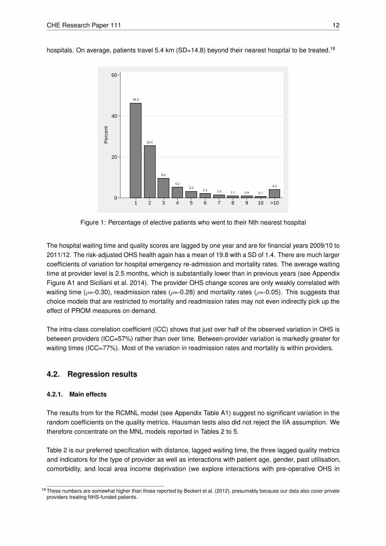
Patients live on average 14.7 kilometres from their chosen hospital. Figure 1 shows that just over half(53.7%) of patients bypassed the local hospital and nearly a fifth (18.3%) bypassed the nearest three
16 The number of providers varied slightly over this period because of mergers, changes in coding and market entry, especially withrespect to private facilities. There were 157 providers in 2010/11, 202 in 2011/12, and 212 in 2012/13, of which 18 (11.5%) in2010/11, 62 (30.7%) in 2011/12, and 78 (36.8%) in 2012/13 are privately operated.
17 We also calculated the correlations between these measures and the EQ-5D utility score, which one may argue is a more holisticmeasure of health-related quality of life. The correlations are similar: ρ = -0.10 for past utilisation, and ρ = -0.14 for comorbidityburden.
CHE Research Paper 111 12
hospitals. On average, patients travel 5.4 km (SD=14.8) beyond their nearest hospital to be treated.18
46.3
25.4
9.5
5.23.2
2.1 1.5 1.1 0.9 0.7
4.0
0
20
40
60
Per
cent
1 2 3 4 5 6 7 8 9 10 >10
Figure 1: Percentage of elective patients who went to their Nth nearest hospital
The hospital waiting time and quality scores are lagged by one year and are for financial years 2009/10 to2011/12. The risk-adjusted OHS health again has a mean of 19.8 with a SD of 1.4. There are much largercoefficients of variation for hospital emergency re-admission and mortality rates. The average waitingtime at provider level is 2.5 months, which is substantially lower than in previous years (see AppendixFigure A1 and Siciliani et al. 2014). The provider OHS change scores are only weakly correlated withwaiting time (ρ=-0.30), readmission rates (ρ=-0.28) and mortality rates (ρ=-0.05). This suggests thatchoice models that are restricted to mortality and readmission rates may not even indirectly pick up theeffect of PROM measures on demand.
The intra-class correlation coefficient (ICC) shows that just over half of the observed variation in OHS isbetween providers (ICC=57%) rather than over time. Between-provider variation is markedly greater forwaiting times (ICC=77%). Most of the variation in readmission rates and mortality is within providers.
4.2. Regression results
4.2.1. Main effects
The results from for the RCMNL model (see Appendix Table A1) suggest no significant variation in therandom coefficients on the quality metrics. Hausman tests also did not reject the IIA assumption. Wetherefore concentrate on the MNL models reported in Tables 2 to 5.
Table 2 is our preferred specification with distance, lagged waiting time, the three lagged quality metricsand indicators for the type of provider as well as interactions with patient age, gender, past utilisation,comorbidity, and local area income deprivation (we explore interactions with pre-operative OHS in
18 These numbers are somewhat higher than those reported by Beckert et al. (2012), presumably because our data also cover privateproviders treating NHS-funded patients.
Do patients choose hospitals that improve their health? 13
section 4.2.2). This specification does not include hospital FEs. The main effects are the estimatedmarginal utilities for the reference patient with mean or modal characteristics. The reference patientprefers shorter distances with the marginal disutility from distance declining with distance. She prefersspecialised providers to non-specialised providers. She is also more likely to choose a public providerover a private provider after accounting for distance, waiting time and quality19.
Reference patient demand is increasing with the OHS change score and falling with emergency admissionrates20. The estimated WTT for a one SD increase in OHS is 1.3 km or 8.7% of the average distancetravelled to the chosen provider. The WTT for a SD decrease in emergency readmission rates is 1.0km.There is no statistically significant effect of procedure-specific mortality rates on demand. Nor does thewaiting time affect choice of provider, which may be a result of the historically short waiting time duringour study period.
Results are robust to the use of contemporaneous rather than lagged waiting time and quality (AppendixTable A2, model 1). Contemporaneous waiting time has a positive but statistically insignificant coefficient.When we use the proportion of patients waiting longer than 120 days as a waiting time measure thecoefficient is negative and statistically significant (Appendix Table A2, model 2). The coefficients on thequality measures are almost unaffected by the use of contemporaneous waiting time and quality.
The HSCIC also produces hospital quality scores based on the case-mix adjusted change in the EQ-5Dutility score. This is highly correlated with the OHS change score (Neuburger et al. 2013) and whenwe estimate the baseline specification with EQ-5D substituted for OHS we find similar WTT (AppendixTable A2, model 3). Results are also robust to exclusion of independent sector treatment centres frompatient choice sets (Appendix Table A2, model 4).
4.2.2. Patient heterogeneity
The coefficients on the interaction terms in the lower parts of Table 2 suggest that preferences varyacross types of patient. We find, like other studies (Propper et al. 2007; Beckert et al. 2012), thatolder patients dislike distance more. They care less about waiting time and get greater marginal utilityfrom improvements in the OHS change score, reductions in emergency readmissions and reductions inmortality rates. There is little difference between the preferences of male and female patients exceptthat male patients have a greater dislike for providers with higher mortality. Preferences vary little bymorbidity as measured by past emergency admissions. In contrast, patients with more comorbiditieshave a greater dislike of distance and waiting time, but care less about readmission rates. Finally, patientsfrom neighbourhoods with greater income deprivation care more about distance and less about quality.
The existence of detailed patient reported pre-operative health status measures in our dataset allows usto explore in more detail whether patients in worse health status are more sensitive to quality and morewilling to travel, as commonly assumed in the literature on hospital quality (Gowrisankaran and Town1999; Geweke et al. 2003). The correlations between patients’ pre-operative OHS and their routinelyavailable morbidity measures are low, suggesting that they measure different aspects of the patient’s
19 During our study period ISTC were funded through block contracts and paid to provide care to a pre-specified number of NHSpatients. However, most ISTCs did not fulfil their quotas although they generally had low waiting times (Naylor and Gregory2009). Our results are consistent with this observation and suggest a positive preference for public providers by NHS-funded hipreplacement patients.
20 We also tested for a non-linear effect of PROM quality on demand by including a squared term for the provider OHS change scores(Ruwaard and Douven 2014). The square term was statistically significant and negative but there was little difference between thelinear and non-linear models over the observed range of values.
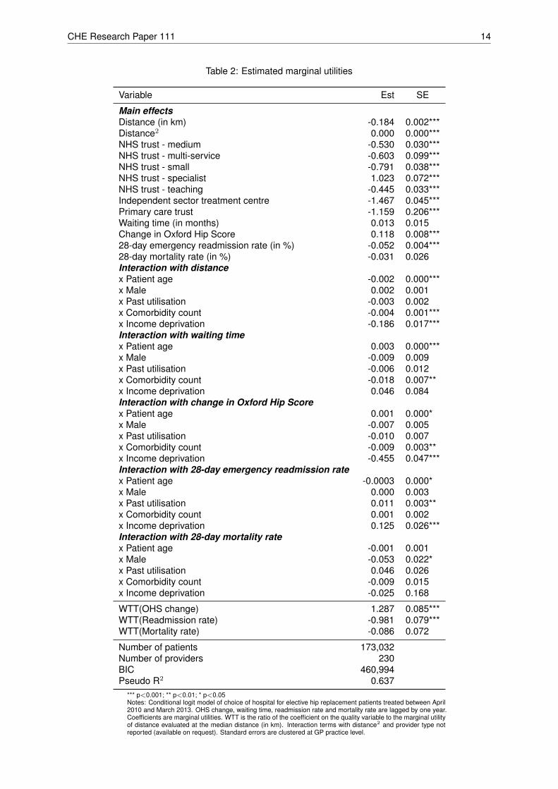
CHE Research Paper 111 14
Table 2: Estimated marginal utilities
Variable Est SE
Main effectsDistance (in km) -0.184 0.002***Distance2 0.000 0.000***NHS trust - medium -0.530 0.030***NHS trust - multi-service -0.603 0.099***NHS trust - small -0.791 0.038***NHS trust - specialist 1.023 0.072***NHS trust - teaching -0.445 0.033***Independent sector treatment centre -1.467 0.045***Primary care trust -1.159 0.206***Waiting time (in months) 0.013 0.015Change in Oxford Hip Score 0.118 0.008***28-day emergency readmission rate (in %) -0.052 0.004***28-day mortality rate (in %) -0.031 0.026Interaction with distancex Patient age -0.002 0.000***x Male 0.002 0.001x Past utilisation -0.003 0.002x Comorbidity count -0.004 0.001***x Income deprivation -0.186 0.017***Interaction with waiting timex Patient age 0.003 0.000***x Male -0.009 0.009x Past utilisation -0.006 0.012x Comorbidity count -0.018 0.007**x Income deprivation 0.046 0.084Interaction with change in Oxford Hip Scorex Patient age 0.001 0.000*x Male -0.007 0.005x Past utilisation -0.010 0.007x Comorbidity count -0.009 0.003**x Income deprivation -0.455 0.047***Interaction with 28-day emergency readmission ratex Patient age -0.0003 0.000*x Male 0.000 0.003x Past utilisation 0.011 0.003**x Comorbidity count 0.001 0.002x Income deprivation 0.125 0.026***Interaction with 28-day mortality ratex Patient age -0.001 0.001x Male -0.053 0.022*x Past utilisation 0.046 0.026x Comorbidity count -0.009 0.015x Income deprivation -0.025 0.168
WTT(OHS change) 1.287 0.085***WTT(Readmission rate) -0.981 0.079***WTT(Mortality rate) -0.086 0.072
Number of patients 173,032Number of providers 230BIC 460,994Pseudo R2 0.637
*** p<0.001; ** p<0.01; * p<0.05Notes: Conditional logit model of choice of hospital for elective hip replacement patients treated between April2010 and March 2013. OHS change, waiting time, readmission rate and mortality rate are lagged by one year.Coefficients are marginal utilities. WTT is the ratio of the coefficient on the quality variable to the marginal utilityof distance evaluated at the median distance (in km). Interaction terms with distance2 and provider type notreported (available on request). Standard errors are clustered at GP practice level.

Do patients choose hospitals that improve their health? 15
condition at the time of admission.
The first model in Table 3 is the same as our preferred specification but with additional patient pre-operative OHS interactions. Interaction terms with other patient characteristics are suppressed for brevity.Due to data limitations, we focus on patients treated during April 2010 and March 2012. We find thathealthier patients are more willing to travel. Although the marginal utility from higher quality is similar forhealthier patients, the reduced distance cost for these patients implies they are more willing to travel forhigher quality. Healthier patients are also more likely to choose a private provider, which is consistentwith observed differences in intake across provider types (Browne et al. 2008).
The fact that pre-operative OHS data are available for only about 60% of patients raises concernsabout response bias if unobserved factors affect propensity to respond and utility from providers21.To investigate if responders to the pre-operative PROM questionnaire have different preferences tonon-responders we re-estimate the preferred specification of Table 2 for our full sample (respondersand non-responders) but interact a dummy variable for responder status with all the main and interactedexplanatory variables; pre-operative health status is not modelled.
The pre-operative PROM questionnaire is administered after the patient has chosen the provider. Hence,it is unclear whether the response indicator variable reflects patient preferences or whether the choicedetermines the response indicator. For example, private providers have higher response rates than NHShospitals (Gomes et al. forthcoming; Gutacker, Street et al. forthcoming) and also tend to have higherobserved quality and shorter waiting times. We address this concern by including the observed providerpre-operative response rate as a provider characteristic when modelling the choices of responders andnon-responders. This variable is informative about the individual’s propensity to fill in a pre-operativePROM questionnaire given the chosen provider22. We find that responders and non-responders havegenerally very similar revealed preferences, with the exception of preferences for waiting times (non-responders prefer shorter waiting times) and PROM quality (responders derive more utility from healthgains and are thus more willing to travel for it). There is no difference with respect to the disutility fromtravel distance, readmission rates or mortality.
4.3. Omitted variable bias
We also explore the possible impact of omitted hospital characteristics on our estimates of marginalutility for quality and other hospital characteristics. We compare preferences of elective and emergencypatients estimated from pooled choice models with a full set of emergency patient dummy variablesinteracted with all explanatory variables. There are 73,629 emergency patients in our sample. Only 20%of emergency patients bypassed the nearest provider (see Appendix Figure A2). Descriptive statistics forthis patient group are reported in Appendix Table A3. Emergency patients’ choice sets are the 50 closestproviders who carried out hip replacement surgery on at least 30 emergency patients in this year. Thisrules out private and specialised providers who only treat elective hip replacement patients. 708 (1.0%)emergency patients were dropped because they attended a provider not in their choice set. All maineffects still pertain to the elective reference patient.
21 We are not concerned about the implications of response rates for the hospital level case-mix adjusted OHS change scores asthese have been shown to be robust to variations in response rate (Gomes et al. forthcoming)
22 As a check, we first re-estimate the responder only model with the addition of provider pre-operative response rates. The resultsare robust to this sensitivity analysis, with the WTT of 1.4km (SE=0.102) for a standard deviation increase in PROM quality beingslightly larger than in our preferred specification (full results available on request).

CH
ER
esea
rch
Pap
er11
116
Table 3: Choice models allowing for patient pre-operative Oxford Hip Score
Patients with pre-opOHS (1)
Patients with pre-opOHS (2)
All patients (3)
Responders (3a) Non-responders (3b) Difference (3c)
Variable Est SE Est SE Est SE Est SE Est SE
Main effectsDistance (in km) -0.185 0.002*** -0.185 0.002*** -0.185 0.002*** -0.188 0.007*** 0.003 0.007Distance2 0.000 0.000*** 0.000 0.000*** 0.000 0.000*** 0.000 0.000** 0.000 0.000NHS trust - medium -0.526 0.037*** -0.646 0.037*** -0.641 0.037*** -0.558 0.039*** -0.083 0.034*NHS trust - multi-service -0.902 0.133*** -0.973 0.131*** -0.965 0.130*** -0.519 0.104*** -0.446 0.123***NHS trust - small -0.820 0.045*** -0.907 0.045*** -0.902 0.044*** -0.857 0.045*** -0.045 0.041NHS trust - specialist 1.052 0.079*** 0.869 0.082*** 0.856 0.082*** 0.973 0.089*** -0.117 0.070NHS trust - teaching -0.445 0.039*** -0.503 0.039*** -0.489 0.039*** -0.608 0.039*** 0.119 0.038**Independent sector treatment centre -1.373 0.065*** -1.499 0.063*** -1.515 0.063*** -1.670 0.067*** 0.155 0.059**Primary care trust -0.978 0.223*** -1.301 0.223*** -1.298 0.224*** -1.272 0.235*** -0.026 0.232Waiting time (in months) -0.011 0.020 0.035 0.020 0.033 0.020 -0.054 0.023* 0.087 0.018***Change in Oxford Hip Score 0.161 0.010*** 0.139 0.010*** 0.137 0.010*** 0.104 0.011*** 0.033 0.010**28-day emergency readmission rate (in %) -0.050 0.006*** -0.046 0.006*** -0.046 0.006*** -0.052 0.006*** 0.006 0.00628-day mortality rate (in %) -0.135 0.035*** -0.068 0.032* -0.067 0.032* -0.014 0.036 -0.053 0.033Response rate 2.044 0.093*** 2.038 0.092*** -2.287 0.080*** 4.325 0.086***Interaction with pre-operative Oxford Hip Scorex Distance (in km) 0.001 0.000*** 0.001 0.000***x Distance2 0.000 0.000*** 0.000 0.000***x NHS trust - medium 0.000 0.002 -0.001 0.002x NHS trust - multi-service -0.004 0.007 -0.006 0.007x NHS trust - small -0.002 0.002 -0.002 0.002x NHS trust - specialist 0.017 0.004*** 0.016 0.004***x NHS trust - teaching -0.005 0.002* -0.008 0.002***x Independent sector treatment centre 0.038 0.003*** 0.035 0.003***x Primary care trust -0.002 0.008 -0.005 0.008x Waiting time (in months) 0.004 0.001*** 0.004 0.001***x Change in Oxford Hip Score 0.001 0.001* 0.000 0.001x 28-day emergency readmission rate (in %) 0.000 0.000 0.000 0.000x 28-day mortality rate (in %) 0.002 0.002 0.003 0.002x Response rate 0.020 0.005***
WTT(OHS change) 1.717 0.111*** 1.475 0.113*** 1.465 0.112*** 1.048 0.136*** 0.417 0.133**WTT(Readmission rate) -0.941 0.107*** -0.867 0.105*** -0.879 0.105*** -0.932 0.132*** 0.054 0.127WTT(Mortality rate) -0.474 0.122*** -0.238 0.112* -0.224 0.107* -0.045 0.113 -0.180 0.107
Number of patients 71,329 71,329 113,751Number of providers 206 206 206BIC 182,407 179,628 283,989Pseudo R2 0.649 0.654 0.657
*** p<0.001; ** p<0.01; * p<0.05Notes: Conditional logit model of choice of hospital for elective hip replacement patients treated between April 2010 and March 2012. OHS change, waiting time, readmission rate and mortality rateare lagged by one year. Coefficients are marginal utilities. WTT is the ratio of the coefficient on the quality variable to the marginal utility of distance evaluated at the median distance (in km). Modelsin (1) and (2) are for patients reporting a pre-operation OHS. Model in (3) is for all patients and interacts a dummy variable for reporting a pre-operation OHS. Interaction effects are reported in (3c).All models also contain a full set of interactions of age, gender, past utilisation, Elixhauser comorbidities, and deprivation with hospital characteristics and distance (not reported). Standard errors areclustered at GP practice level.

Do patients choose hospitals that improve their health? 17
We report results for two different specifications. The first model in Table 4 compares emergency patientswith elective patients who choose NHS or independent providers. However, there are some markeddifferences in observed characteristics between those two groups. For example, emergency patients areon average 12 years older than elective patients and have over twice as many recorded comorbidities.Hence in the second model reported in Table 5 we compare a set of elective and emergency patientsmatched exactly on age, gender, past emergency admissions, number of comorbidities, income depriva-tion and year of treatment. Additionally, we restrict the elective patient sample to those who used anNHS provider that treats at least 30 elective and emergency patients in that year; hence the choice setsare identical for elective and emergency conditional on location.
Table 4: Comparison of marginal utilities for elective and emergency patients
Elective patients Emergency patients Difference
Variable Est SE Est SE Est SE
Distance (in km) -0.184 0.002*** -0.217 0.004*** -0.033 0.003***Distance2 0.000 0.000*** 0.001 0.000*** 0.000 0.000***NHS trust - medium -0.530 0.030*** -0.571 0.045*** -0.041 0.039NHS trust - multi-service -0.603 0.099*** -0.935 0.164*** -0.332 0.145*NHS trust - small -0.791 0.038*** -0.823 0.050*** -0.032 0.044NHS trust - specialist 1.023 0.072*** n/a n/aNHS trust - teaching -0.445 0.033*** -0.609 0.045*** -0.164 0.042***Independent sector treatment centre -1.467 0.045*** n/a n/aPrimary care trust -1.159 0.206*** -1.274 0.258*** -0.115 0.176Waiting time (in months) 0.013 0.015 -0.010 0.022 -0.023 0.021Change in Oxford Hip Score 0.118 0.008*** 0.048 0.013*** -0.070 0.012***28-day emergency readmission rate (in %) -0.052 0.004*** -0.046 0.008*** 0.006 0.00728-day mortality rate (in %) -0.031 0.026 0.056 0.056 0.087 0.057
WTT(OHS change) 1.285 0.085*** 0.523 0.143*** -0.763 0.126***WTT(Readmission rate) -0.978 0.079*** -0.870 0.150*** 0.109 0.134WTT(Mortality rate) -0.085 0.072 0.155 0.155 0.241 0.157
Number of patients 173,032 72,921Number of providers 230 138BIC 570,669Pseudo R2 0.689
*** p<0.001; ** p<0.01; * p<0.05Notes: Conditional logit model of choice of hospital for elective and emergency hip replacement patients treated between April 2010 and March2013. OHS change, waiting time, readmission rate and mortality rate are lagged by one year. Coefficients are marginal utilities for the ‘referencepatient’. Elective and emergency patients are not matched on observed characteristics but the ‘reference patient’ in both patient populations isdefined according to the average characteristics of the elective patient sample. WTT is the ratio of the coefficient on the quality variable to themarginal utility of distance evaluated at the median distance (in km). Model is estimated with a full set of dummy variables interacted with hospitalcharacteristics and other interaction terms. All models also contain a full set of interactions of age, gender, past utilisation, Elixhauser comorbidities,and deprivation with hospital characteristics and distance (not reported). Standard errors are clustered at GP practice level.

CHE Research Paper 111 18
Table 5: Comparison of marginal utilities for elective and emergency patients - matched sample
Elective patients Emergency patients Difference
Variable Est SE Est SE Est SE
Distance (in km) -0.220 0.004*** -0.215 0.004*** 0.005 0.005Distance2 0.001 0.000*** 0.000 0.000*** 0.000 0.000***NHS trust - medium -0.709 0.050*** -0.560 0.046*** 0.149 0.053**NHS trust - multi-service -0.710 0.175*** -0.921 0.182*** -0.211 0.213NHS trust - small -0.880 0.058*** -0.794 0.053*** 0.086 0.062NHS trust - teaching -0.468 0.053*** -0.598 0.048*** -0.130 0.058*Primary care trust -1.133 0.292*** -1.429 0.314*** -0.296 0.282Waiting time (in months) -0.087 0.027** -0.032 0.024 0.055 0.029Change in Oxford Hip Score 0.092 0.015*** 0.034 0.014* -0.058 0.016***28-day emergency readmission rate (in %) -0.061 0.009*** -0.046 0.008*** 0.015 0.01028-day mortality rate (in %) -0.050 0.061 0.070 0.063 0.120 0.079
WTT(OHS change) 0.796 0.128*** 0.354 0.142* -0.441 0.149**WTT(Readmission rate) -0.893 0.129*** -0.814 0.152*** 0.079 0.165WTT(Mortality rate) -0.084 0.102 0.140 0.127 0.224 0.148
Number of patients 32,274 32,274Number of providers 138 138BIC 107,831Pseudo R2 0.771
*** p<0.001; ** p<0.01; * p<0.05Notes: Conditional logit model of choice of hospital for elective and emergency hip replacement patients treated between April 2010 and March 2013.OHS change, waiting time, readmission rate and mortality rate are lagged by one year. Coefficients are marginal utilities for the ‘reference patient’.Elective and emergency patients are matched exactly on observed characteristics (age, gender, past emergency utilisation in last year (none, once,or more), income deprivation of neighbourhood, number of Elixhauser comorbit conditions, year of treatment) and the ‘reference patient’ in bothpatient populations is defined according to the average (prior to matching) characteristics of the elective patient sample. Choice sets include onlyproviders that treat at least 30 elective and 30 emergency hip replacement patient in this period. WTT is the ratio of the coefficient on the qualityvariable to the marginal utility of distance evaluated at the median distance (in km). Model is estimated with a full set of dummy variables interactedwith hospital characteristics and other interaction terms. All models also contain a full set of interactions of age, gender, past utilisation, Elixhausercomorbidities, and deprivation with hospital characteristics and distance (not reported). Standard errors are clustered at GP practice level.
Both models suggest that emergency patients care less about provider OHS changes but have similarpreferences over the more traditional quality measures using readmission and mortality rates. In thesecond specification, with closely matched patients, the estimated marginal utility of OHS changes(βEmer
q =0.034) is just over one third of that for elective patients (βElecq =0.092) and significant at p<0.05.
If we assume that emergency patients’ demand is entirely inelastic to variation in observed electivequality and that the estimated association for emergency patients is a result of omitted variables thataffect emergency and elective patients in the same way, then the difference in the marginal utility of OHSchanges (β∆
q =0.058) can be interpreted as a lower bound estimate of the true effect of OHS changescore on elective patient utility. The WTT for a one SD increase in OHS change scores then is 0.4km(SE=0.149), which is smaller than that reported in Table 2.
Table 6 shows the main effects from our preferred specification estimated with additional hospital FEs.We find that PROM quality still has a statistically significant effect on demand, whereas emergencyreadmission rates no longer do. The WTT to travel for PROM quality is however 87% lower than thatcalculated from the results in Table 2 (0.2km vs 1.3km). This is likely to be due to the fixed effectabsorbing part of the effect of time-invariant quality on choice. Results are broadly similar when patients’choice sets are restricted to NHS hospitals, although we now find a counter-intuitive positive effect ofwaiting time on demand.

Do patients choose hospitals that improve their health? 19
Table 6: Choice model controlling for unobserved time-invariant hospital effects
All providers (1) NHS providers only (2)
Est SE Est SE
Distance (in km) -0.202 0.002*** -0.231 0.003***Distance2 0.000 0.000*** 0.001 0.000***Waiting time (in months) 0.021 0.024 0.053 0.012***Change in Oxford Hip Score 0.017 0.006** 0.016 0.007*28-day emergency readmission rate (in %) 0.005 0.004 0.000 0.00428-day mortality rate (in %) 0.038 0.020 0.021 0.026
WTT(OHS change) 0.168 0.060** 0.124 0.055*WTT(Readmission rate) 0.089 0.066 -0.0001 0.053WTT(Mortality rate) 0.095 0.051 0.031 0.039
Number of patients 173,032 148,629Number of providers 230 144BIC 411,541 260,299Pseudo R2 0.678 0.742
*** p<0.001; ** p<0.01; * p<0.05Notes: Conditional logit model of choice of hospital for elective hip replacement patients treated between April 2010 andMarch 2013. OHS change, waiting time, readmission rate and mortality rate are lagged by one year. Coefficients aremarginal utilities. WTT is the ratio of the coefficient on the quality variable to the marginal utility of distance evaluated atthe median distance (in km). Model in (1) does not impose restrictions on the type of provider in patients’ choice sets.Model in (2) is based on a restricted choice set of NHS providers, thereby excluding patients that selected ISTCs. Allmodels include indicator variables for hospitals (not reported). All models also contain a full set of interactions of age,gender, past utilisation, Elixhauser comorbidities, and deprivation with hospital characteristics and distance (not reported).Standard errors are clustered at GP practice level.
CHE Research Paper 111 20
5. The economic effects of quality on demand
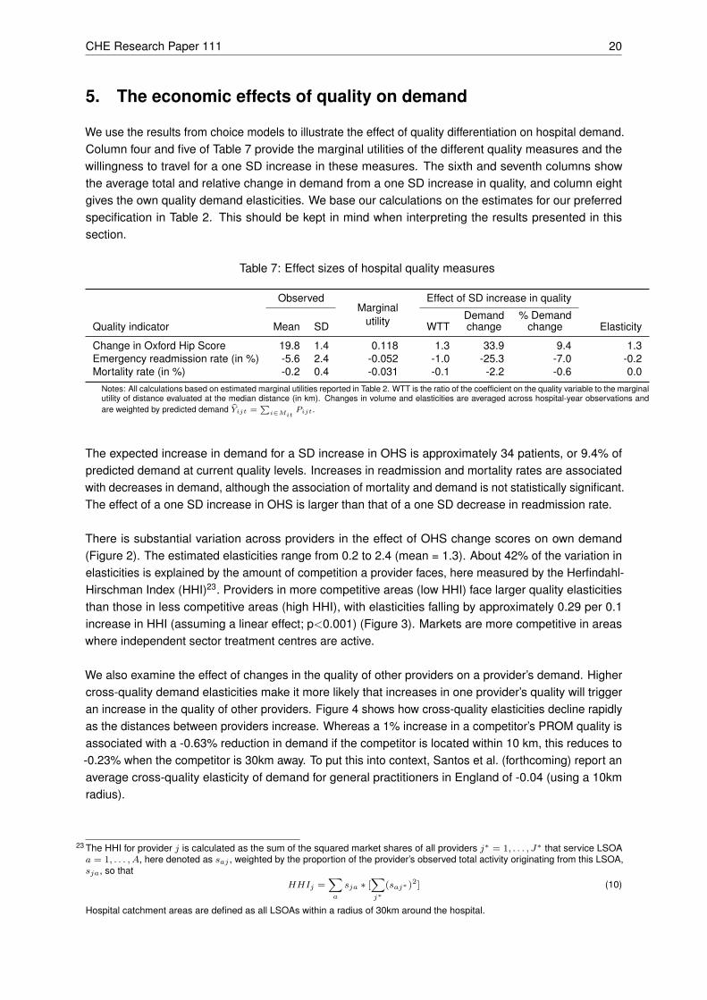
We use the results from choice models to illustrate the effect of quality differentiation on hospital demand.Column four and five of Table 7 provide the marginal utilities of the different quality measures and thewillingness to travel for a one SD increase in these measures. The sixth and seventh columns showthe average total and relative change in demand from a one SD increase in quality, and column eightgives the own quality demand elasticities. We base our calculations on the estimates for our preferredspecification in Table 2. This should be kept in mind when interpreting the results presented in thissection.
Table 7: Effect sizes of hospital quality measures
ObservedMarginal
utility
Effect of SD increase in quality
Quality indicator Mean SD WTTDemandchange
% Demandchange Elasticity
Change in Oxford Hip Score 19.8 1.4 0.118 1.3 33.9 9.4 1.3Emergency readmission rate (in %) -5.6 2.4 -0.052 -1.0 -25.3 -7.0 -0.2Mortality rate (in %) -0.2 0.4 -0.031 -0.1 -2.2 -0.6 0.0
Notes: All calculations based on estimated marginal utilities reported in Table 2. WTT is the ratio of the coefficient on the quality variable to the marginalutility of distance evaluated at the median distance (in km). Changes in volume and elasticities are averaged across hospital-year observations andare weighted by predicted demand Yijt =
∑i∈Mit
Pijt.
The expected increase in demand for a SD increase in OHS is approximately 34 patients, or 9.4% ofpredicted demand at current quality levels. Increases in readmission and mortality rates are associatedwith decreases in demand, although the association of mortality and demand is not statistically significant.The effect of a one SD increase in OHS is larger than that of a one SD decrease in readmission rate.
There is substantial variation across providers in the effect of OHS change scores on own demand(Figure 2). The estimated elasticities range from 0.2 to 2.4 (mean = 1.3). About 42% of the variation inelasticities is explained by the amount of competition a provider faces, here measured by the Herfindahl-Hirschman Index (HHI)23. Providers in more competitive areas (low HHI) face larger quality elasticitiesthan those in less competitive areas (high HHI), with elasticities falling by approximately 0.29 per 0.1increase in HHI (assuming a linear effect; p<0.001) (Figure 3). Markets are more competitive in areaswhere independent sector treatment centres are active.
We also examine the effect of changes in the quality of other providers on a provider’s demand. Highercross-quality demand elasticities make it more likely that increases in one provider’s quality will triggeran increase in the quality of other providers. Figure 4 shows how cross-quality elasticities decline rapidlyas the distances between providers increase. Whereas a 1% increase in a competitor’s PROM quality isassociated with a -0.63% reduction in demand if the competitor is located within 10 km, this reduces to-0.23% when the competitor is 30km away. To put this into context, Santos et al. (forthcoming) report anaverage cross-quality elasticity of demand for general practitioners in England of -0.04 (using a 10kmradius).
23 The HHI for provider j is calculated as the sum of the squared market shares of all providers j∗ = 1, . . . , J∗ that service LSOAa = 1, . . . , A, here denoted as saj , weighted by the proportion of the provider’s observed total activity originating from this LSOA,sja, so that
HHIj =∑a
sja ∗ [∑j∗
(saj∗ )2] (10)
Hospital catchment areas are defined as all LSOAs within a radius of 30km around the hospital.

Do patients choose hospitals that improve their health? 21
05
1015
20P
erce
nt
0 50 100 150Patients
Absolute volume effect
02
46
810
Per
cent
0 5 10 15% increase
Relative volume effect
02
46
8P
erce
nt
0 .5 1 1.5 2 2.5% increase
Elasticity
Figure 2: Distribution of changes in hospital demand as a result of a SD increase in Oxford HipScore change scores and quality elasticity of demand
.51
1.5
22.
5E
last
icity
of o
wn
dem
and
to q
ualit
y
.5 .6 .7 .8 .9 1Weighted provider HHI
ISTC NHS
Figure 3: Differences in quality elasticity of demand between providers in competitive (low HHI) andnon-competitive (high HHI) markets

CHE Research Paper 111 22
-2-1
.5-1
-.5
0C
ross
-ela
stic
ity
0 10 20 30Distance between providers
Figure 4: Percentage change in demand as a result of percentage change in competitor’s quality
Do patients choose hospitals that improve their health? 23
6. Discussion and concluding remarks
The collection of patient-reported outcome measures has been introduced in England with the ambitionthat these new metrics of hospital quality would influence patient choice of hospital (Department of Health2008). This paper is the first to test the relationship between observed hospital PROM quality and demandfor elective hip replacement surgery. It uses data on observed choices for all NHS-funded patients treatedbetween April 2010 and March 2013 in private and public hospitals in England. In order to addresspotential endogeneity bias we implement an empirical strategy based on lagged explanatory variables,hospital fixed effects and a control group design based on demand for emergency hip replacement.
Our results suggest that elective hospital demand is statistically significantly associated with observedquality as measured by PROMs and other metrics. While individual patients are not very sensitive toquality differences - the estimated willingness to travel for a standard deviation increase in PROM qualityis less than 1.3km - the number of potential patients in a hospital’s market implies that hospitals canattract an increase in elective activity of approximately 34 new patients, or 9% of existing activity levels, ifthey find ways to improve PROM quality by one standard deviation. Hospital demand is more responsiveto a one standard deviation of PROM quality than one standard deviation of emergency readmissionrates, and there is no statistically significant association with mortality rates after hip replacement surgery.
Our findings that choice responds to quality suggest that providers could compete on quality. However,the change in activity that would arise after a change in quality may be modest. First, a standard deviationincrease in OHS (equivalent to 1.4 points) would be a substantial improvement in quality for any providerand difficult to achieve. For comparison, the average year-on-year improvement in hospital PROM scoresis 0.196 OHS points, or less than 15% of the observed standard deviation. Second, we show that theeffect of quality changes on the providers’ ability to attract patients away from local competitors diminishesrapidly as distance increases. This may result in local quasi-monopolies where quality improvementshave little effect on demand. Finally, our estimated effect is likely to be an upper bound estimate andour analysis on emergency patients suggests that the coefficient of demand to quality could be up to30% smaller. Taken together, the incentive effect of patients ‘voting with their feet’ and demanding higherquality is likely to be limited.
There are several policy levers which may be used to ensure that PROM quality information is used toinform hospital choice (Marshall et al. 2004; Faber et al. 2009). Many patients may still not know abouthospital PROM scores and more active dissemination to the general public may be required (e.g. byadding the information to the Choose & Book system). Some patients may find it difficult to access thisinformation, for example if they do not have access to the internet. There is a lack of evidence on theextent to which patients and general practitioners are aware of this information and consider it as part oftheir decision-making process. Similarly, the information may not be sufficiently meaningful to them inits current format. A recent study by Hildon et al. (2012) showed that a high proportion of patients anddoctors do not consider the reported PROMs to have an intuitive metric and thus struggle to interpretprovider scores. Finally, some patients may not consider variation between hospitals sufficiently large tobe considered important. Some of these points may resolve over time, whereas others require targetedpolicy intervention to improve the dissemination of quality information.
We also explore whether patient preferences vary according to observed and unobserved patientcharacteristics. We find that the preference for PROM quality increases with age and decreases withincome deprivation, comorbidity burden and past utilisation. Qualitatively similar results are obtainedfor preferences for quality as approximated by emergency readmission rates. Interestingly, we do not

CHE Research Paper 111 24
find evidence that preferences for quality vary with pre-operative health status as reported by the patientherself. But because healthier patients are more willing to travel, they have ceteris paribus a higherwillingness to travel for quality. Hence, the ‘distance bias’ described by Gowrisankaran and Town (1999)is likely to occur not because more morbid patients request higher quality, but because they derivedifferent disutility from travel. This finding may be specific to the condition under study as osteoarthritisand other conditions that require hip replacement reduce patients’ mobility, and more severely morbidpatients thus may be less able or willing to travel.
There remains scope for further research. For example, we cannot disentangle whether the estimatedeffect is driven by patients’ choices versus general practitioners choices acting on their behalf. Weconjecture it is due to both. We also did not test whether the first release of PROM information in 2009/10constituted news to patients and how this impacted on providers’ demand.
In conclusion, the results in this paper provide some first evidence to suggest that hospital demand forhip replacement responds to hospital quality as captured by changes in patient-reported health status.

Do patients choose hospitals that improve their health? 25
References
Appleby, J. and N. Devlin (2004). Measuring success in the NHS: using patient assessed health outcomesto manage the performance of health care providers. The King’s Fund. London.
Beckert, W., M. Christensen and K. Collyer (2012). ‘Choice of NHS-funded hospital services in England’.The Economic Jounal 122, 400–417.
Belmont, P. J., G. P. Goodman, B. R. Waterman, J. O. Bader and A. J. Schoenfeld (2014). ‘Thirty-DayPostoperative Complications and Mortality Following Total Knee Arthroplasty - Incidence and RiskFactors Among a National Sample of 15,321 Patients’. The Journal of Bone & Joint Surgery 96 (1),20–26.
Berstock, J. R., A. D. Beswick, E. Lenguerrand, M. R. Whitehouse and A. W. Blom (2014). ‘Mortality aftertotal hip replacement surgery: A systematic review’. Bone and Joint Research 3 (6), 175–182.
Besley, T. and M. Ghatak (2003). ‘Incentives, Choice, and Accountability in the Provision of PublicServices’. Oxford Review of Economic Policy 19 (2), 235–249.
Brekke, K., H. Gravelle, L. Siciliani and O. Straume (2014). ‘Patient Choice, Mobility and CompetitionAmong Health Care Providers’. In: Health Care Provision and Patient Mobility. Ed. by R. Levaggi andM. Montefiori. Springer.
Brooks, R. (1996). ‘EuroQol: the current state of play’. Health Policy 37, 53–72.Browne, J., L. Jamieson, J. Lewsey, J. van der Meulen, L. Copley and N. Black (2008). ‘Case-mix
& patients’ reports of outcome in Independent Sector Treatment Centres: Comparison with NHSproviders’. BMC Health Services Research 8 (1), 78.
Commission on the Future of Health and Social Care in England (2014). The UK private health market.Appendix to ‘A new settlement for Health and Social Care’. London: The King’s Fund.
Dawson, J., R. Fitzpatrick, A. Carr and D. Murray (1996). ‘Questionnaire on the perceptions of patientsabout total hip replacement’. Journal of Bone & Joint Surgery, British Volume 78-B, 185–190.
Department of Health (2008). Guidance on the routine collection of Patient Reported Outcome Measures(PROMs). The Stationary Office, London.
— (2012). Patient Reported Outcome Measures (PROMs) in England: The case-mix adjustment meth-odology. The Stationary Office, London.
Elixhauser, A., C. Steiner, D. Harris and R. Coffey (1998). ‘Comorbidity measures for use with adminis-trative data’. Medical Care 36 (1), 8–27.
Faber, M., M. Bosch, H. Wollersheim, S. Leatherman and R. Grol (2009). ‘Public reporting in health care:how do consumers use quality-of-care information?: A systematic review’. Medical Care 47 (1), 1–8.
Gaynor, M., H. Seider and W. Vogt (2005). ‘The Volume-Outcome Effect, Scale Economies, and Learningby Doing’. American Economic Review 95 (2), 243–247.
Gaynor, M., C. Propper and S. Seiler (2012). Free to Choose? Reform and Demand Response in theEnglish National Health Service. Working Paper 18574. National Bureau of Economic Research.
Geweke, J., G. Gowrisankaran and R. J. Town (2003). ‘Bayesian Inference for Hospital Quality in aSelection Model’. Econometrica 71 (4), 1215–1238.
Gomes, M., N. Gutacker, C. Bojke and A. Street (forthcoming). ‘Addressing missing data in patient-reported outcome measures (PROMs): implications for comparing provider performance.’ HealthEconomics.
Gowrisankaran, G. and R. J. Town (1999). ‘Estimating the quality of care in hospitals using instrumentalvariables’. Journal of Health Economics 18 (6), 747–767.
Gravelle, H., R. Santos and L. Siciliani (2014). ‘Does a hospital’s quality depend on the quality of otherhospitals? A spatial econometrics approach’. Regional Science and Urban Economics 49, 203–216.
CHE Research Paper 111 26
Gutacker, N., K. Bloor and R. Cookson (2015). ‘Comparing the performance of the Charlson/Deyoand Elixhauser comorbidity measures across five European countries and three conditions’. TheEuropean Journal of Public Health 25 (Suppl 1), 15–20.
Gutacker, N., C. Bojke, S. Daidone, N. Devlin and A. Street (2013). ‘Hospital Variation in Patient-ReportedOutcomes at the Level of EQ-5D Dimensions: Evidence from England’. Medical Decision Making33 (6), 804–818.
Gutacker, N., A. Street, M. Gomes and C. Bojke (forthcoming). ‘Should English healthcare providers bepenalised for failing to collect patient-reported outcome measures (PROMs)?’ Journal of the RoyalSociety of Medicine.
Health & Social Care Information Centre (2013a). Emergency readmissions to hospital within 28 days ofdischarge: primary hip replacement surgery. Compendium of Population Health Indicators. Accessedon 24/11/2014. URL: https://indicators.ic.nhs.uk/download/NCHOD/Specification/Spec_33D_533ISP4CPP1_12_V1.pdf.
— (2013b). Finalised Patient Reported Outcome Measures (PROMs) in England: April 2011 to March2012. Accessed on 26/03/2015. URL: http://www.hscic.gov.uk/catalogue/PUB11359/final-proms-eng-apr11-mar12-fin-report-v2.pdf.
Hensher, D. A. and W. H. Greene (2003). ‘The Mixed Logit model: The state of practice’. Transportation30, 133–176.
Hildon, Z., D. Allwood and N. Black (2012). ‘Making data more meaningful. Patients’ views of the formatand content of quality indicators comparing health care providers’. Patient Education and Counseling88, 298–304.
Hodgkin, D. (1996). ‘Specialized service offerings and patients’ choice of hospital: the case of cardiaccatheterization’. Journal of Health Economics 15 (3), 305–332.
Hole, A. R. (2007a). ‘A comparison of approaches to estimating confidence intervals for willingness topay measures’. Health Economics 16 (8), 827–840.
— (2007b). ‘Fitting mixed logit models by using maximum simulated likelihood’. The Stata Journal 7 (3),388–401.
Hunt, L. P., Y. Ben-Shlomo, E. M. Clark, P. Dieppe, A. Judge, A. J. MacGregor, J. H. Tobias, K. Vernonand A. W. Blom (2013). ‘90-day mortality after 409,096 total hip replacements for osteoarthritis, fromthe National Joint Registry for England and Wales: a retrospective analysis’. The Lancet 382 (9898),1097–1104.
Hutchings, A., J. Neuburger, J. van der Meulen and N. Black (2014). ‘Estimating recruitment rates forroutine use of patient reported outcome measures and the impact on provider comparisons.’ BMCHealth Services Research 14 (1), 66.
Iversen, T. and L. Siciliani (2011). ‘Non-price rationing and waiting times’. In: The Oxford Handbook ofHealth Economics. Ed. by S. Glied and P. C. Smith. Oxford: Oxford University Press.
Judge, A., J. Chard, I. Learmonth and P. Dieppe (2006). ‘The effects of surgical volumes and trainingcentre status on outcomes following total joint replacement: analysis of the Hospital Episode Statisticsfor England’. Journal of Public Health 28 (2), 116–124.
Jung, K., R. Feldman and D. Scanlon (2011). ‘Where would you go for your next hospitalization?’ Journalof Health Economics 30 (4), 832–841.
Lilford, R. and P. Pronovost (2010). ‘Using hospital mortality rates to judge hospital performance: a badidea that just won’t go away’. BMJ 340, 955–957.
Luft, H. S., S. S. Hunt and S. C. Maerki (1987). ‘The Volume-Outcome Relationship: Practice-Makes-Perfect or Selective-Referral Patterns?’ Health Services Research 22 (2), 157–182.
Mäkelä, K. T., U. Häkkinen, M. Peltola, M. Linna, H. Kröger and V. Remes (2011). ‘The effect ofhospital volume on length of stay, re-admissions, and complications of total hip arthroplasty’. ActaOrthopaedica 82 (1), 20–26.
Do patients choose hospitals that improve their health? 27
Marshall, M. N., P. S. Romano and H. T. O. Davies (2004). ‘How do we maximize the impact of the publicreporting of quality of care?’ International Journal for Quality in Health Care 16 (S1), 57–63.
McFadden, D. (1974). ‘Conditional logit analysis of qualitative choice behaviour’. In: Frontiers in econom-ics. Ed. by P. Zarembka. Vol. 4. New York: Academic Press, 105–142.
Moja, L., A. Piatti, V. Pecoraro, C. Ricci, G. Virgili, G. Salanti, L. Germagnoli, A. Liberati and G. Banfi(2012). ‘Timing Matters in Hip Fracture Surgery: Patients Operated within 48 Hours Have BetterOutcomes. A Meta-Analysis and Meta-Regression of over 190,000 Patients’. PLoS ONE 7 (10),e46175.
Monstad, K., L. Engester and B. Espehaug (2006). Patient preferences for choice of hospital. Tech. rep.Health Economics Bergen Working Paper No 05/06.
Moscone, F., E. Tosetti and G. Vittadini (2012). ‘Social interaction in patients’ hospital choice: evidencefrom Italy’. Journal of the Royal Statistical Society: Series A (Statistics in Society) 175 (2), 453–472.
Naylor, C. and S. Gregory (2009). ‘Independent sector treatment centres’. The King’s Fund Briefing.Neuburger, J., A. Hutchings, J. van der Meulen and N. Black (2013). ‘Using patient-reported outcomes
(PROs) to compare the provider of surgery: does the choice of measure matter?’ Medical Care 51 (6),517–523.
NICE (2011). Hip fracture: The manamanage of hip fracture in adults. NICE Guidelines 124. London.Noble, M., G. Wright, G. Smith and C. Dibben (2006). ‘Measuring multiple deprivation at the small-area
level’. Environment and Planning A 38 (1), 169–185.Nuttall, D., D. Parkin and N. Devlin (2015). ‘Inter-provider comparison of patient-reported outcomes:
developing an adjustment to account for differences in patient case mix’. Health Economics 24 (1),41–54.
Pope, D. (2009). ‘Reacting to rankings: Evidence from “America’s best hospitals”’. Journal of HealthEconomics 28 (6), 1154–1165.
Propper, C., M. Damiani, G. Leckie and J. Dixon (2007). ‘Impact of patients’ socioeconomic status on thedistance travelled for hospital admission in the English National Health Service’. Journal of HealthServices Research & Policy 12 (3), 153–159.
Ruwaard, S. and R. Douven (2014). Quality and hospital choice for cataract treatments: the winner takesmost. CPB Netherlands Bureau for Economic Policy Analysis.
Santos, R., H. Gravelle and C. Propper (forthcoming). ‘Does quality affect patients’ choice of doctor?Evidence from England’. The Economic Journal.
Siciliani, L., V. Moran and M. Borowitz (2014). ‘Measuring and comparing health care waiting times inOECD countries’. Health Policy 118 (3), 292–303.
Sivey, P. (2008). ‘The effect of hospital quality on choice of hospital for elective heart operations inEngland’. PhD thesis. University of York.
— (2012). ‘The effect of waiting time and distance on hospital choice for English cataract patients’.Health Economics 21, 444–456.
Train, K. E. (2003). Discrete Choice Methods with Simulation. 1st ed. Cambridge: Cambridge UniversityPress.
Varkevisser, M., S. A. Geest and F. T. Schut (2010). ‘Assessing hospital competition when prices don’tmatter to patients: the use of time-elasticities’. International Journal of Health Care Finance andEconomics 10 (1), 43–60.
— (2012). ‘Do patients choose hospitals with high quality ratings? Empirical evidence from the marketfor angioplasty in the Netherlands’. Journal of Health Economics 31 (2), 371–378.
Vrangbaek, K., R. Robertson, U. Winblad, H. Van de Bovenkamp and A. Dixon (2012). ‘Choice policiesin Northern European health systems’. Health Economics, Policy and Law 7 (S1), 47–71.
Wooldridge, J. M. (2002). Econometric Analysis of Cross Section and Panel Data. Cambridge, Mas-sachusetts: MIT Press.

CHE Research Paper 111 28
Appendix
Table A1: Mixed logit choice model
Mean Standard deviation
Variable Est SE Est SE
Distance (in km) -0.184 0.002***Distance2 0.000 0.000***NHS trust - medium -0.530 0.030***NHS trust - multi-service -0.603 0.099***NHS trust - small -0.791 0.038***NHS trust - specialist 1.023 0.072***NHS trust - teaching -0.445 0.033***Independent sector treatment centre -1.467 0.045***Primary care trust -1.159 0.206***Waiting time (in months) 0.013 0.015Change in Oxford Hip Score 0.118 0.008*** 0.000 0.00128-day emergency readmission rate (in %) -0.052 0.004*** 0.000 0.00128-day mortality rate (in %) -0.031 0.026 -0.002 0.005
WTT(OHS change) 1.287 0.085***WTT(Readmission rate) -0.981 0.079***WTT(Mortality rate) -0.086 0.072
Number of patients 173,032Number of providers 230BIC 461,041
*** p<0.001; ** p<0.01; * p<0.05Notes: Random coefficient (mixed) multinomial logit model of choice of hospital for elective hip replacement patientstreated between April 2010 and March 2013. OHS change, waiting time, readmission rate and mortality rate arelagged by one year. Coefficients are marginal utilities. Random coefficients are specified for OHS change, readmis-sion rate and mortality rate and estimates. WTT is the ratio of the coefficient on the quality variable to the marginalutility of distance evaluated at the median distance (in km). Interaction terms with patient characteristics not reported(available on request). Standard errors are clustered at GP practice level. The mean coefficients do differ from thosereported in Table 2 for the conditional logit model if there is less rounding.

Do patients choose hospitals that improve their health? 29
Table A2: Sensitivity analyses
Model (1) Model (2) Model (3) Model (4)
Variable Est SE Est SE Est SE Est SE
Main effectsDistance (in km) -0.183 0.002*** -0.184 0.002*** -0.184 0.002*** -0.207 0.003***Distance2 0.000 0.000*** 0.000 0.000*** 0.000 0.000*** 0.001 0.000***NHS trust - medium -0.508 0.032*** -0.530 0.030*** -0.540 0.031*** -0.643 0.036***NHS trust - multi-service -0.656 0.090*** -0.615 0.099*** -0.612 0.097*** -0.604 0.098***NHS trust - small -0.740 0.037*** -0.792 0.038*** -0.790 0.038*** -0.909 0.042***NHS trust - specialist 1.019 0.071*** 1.002 0.072*** 1.065 0.073*** 1.047 0.083***NHS trust - teaching -0.502 0.033*** -0.432 0.033*** -0.412 0.032*** -0.513 0.037***Independent sector treatment centre -1.472 0.068*** -1.522 0.037*** -1.398 0.044***Primary care trust -1.071 0.200*** -1.153 0.206*** -1.111 0.206*** -1.195 0.213***Waiting time (in months) 0.033 0.018 -0.193 0.076* 0.007 0.015 -0.029 0.018Change in PROM score 0.104 0.007*** 0.115 0.008*** 4.935 0.284*** 0.121 0.010***28-day emergency readmission rate (in %) -0.054 0.004*** -0.052 0.004*** -0.054 0.004*** -0.054 0.006***28-day mortality rate (in %) -0.044 0.024 -0.032 0.026 -0.026 0.026 0.033 0.035Interaction with distancex Patient age -0.001 0.000*** -0.002 0.000*** -0.002 0.000*** -0.002 0.000***x Male 0.001 0.001 0.002 0.001 0.002 0.001 0.005 0.002**x Past utilisation -0.003 0.002 -0.003 0.002 -0.003 0.002 -0.001 0.002x Comorbidity count -0.005 0.001*** -0.004 0.001*** -0.003 0.001*** -0.001 0.001x Income deprivation -0.179 0.015*** -0.186 0.017*** -0.189 0.018*** -0.241 0.022***Interaction with waiting timex Patient age 0.003 0.000*** 0.008 0.002** 0.003 0.000*** 0.003 0.001***x Male -0.018 0.010 -0.068 0.051 -0.010 0.009 0.001 0.012x Past utilisation -0.005 0.012 0.049 0.059 -0.007 0.012 0.008 0.013x Comorbidity count -0.036 0.007*** -0.057 0.033 -0.018 0.007** -0.016 0.007*x Income deprivation 0.032 0.086 1.180 0.458* 0.083 0.084 0.007 0.107Interaction with change in PROM scorex Patient age 0.001 0.000*** 0.001 0.000* 0.047 0.010*** 0.001 0.000x Male 0.004 0.005 -0.007 0.005 -0.300 0.214 -0.002 0.006x Past utilisation -0.014 0.006* -0.008 0.007 -0.327 0.240 -0.012 0.007x Comorbidity count -0.009 0.003** -0.009 0.003** -0.475 0.128*** -0.004 0.004x Income deprivation -0.389 0.046*** -0.448 0.047*** -18.634 1.698*** -0.568 0.056***Interaction with 28-day emergency readmission ratex Patient age 0.000 0.000* 0.000 0.000* 0.000 0.000 -0.001 0.000**x Male 0.002 0.003 0.000 0.003 0.000 0.003 -0.003 0.004x Past utilisation 0.012 0.004** 0.012 0.003*** 0.012 0.004*** 0.010 0.004**x Comorbidity count 0.003 0.002 0.001 0.002 0.001 0.002 0.003 0.002x Income deprivation 0.082 0.026** 0.124 0.026*** 0.138 0.026*** 0.121 0.034***Interaction with 28-day mortality ratex Patient age -0.002 0.001* -0.001 0.001 -0.001 0.001 -0.001 0.001x Male -0.051 0.021* -0.053 0.022* -0.049 0.022* -0.058 0.031x Past utilisation 0.039 0.030 0.049 0.026 0.047 0.026 0.060 0.032x Comorbidity count -0.001 0.015 -0.010 0.015 -0.009 0.015 -0.004 0.018x Income deprivation -0.059 0.172 -0.023 0.168 -0.049 0.167 -0.230 0.210
WTT(PROM change) 1.174 0.086*** 1.261 0.086*** 1.284 0.076*** 1.078 0.089***WTT(Readmission rate) -1.042 0.081*** -0.983 0.080*** -1.034 0.079*** -0.824 0.089***WTT(Mortality rate) -0.125 0.067 -0.091 0.073 -0.074 0.074 0.055 0.059
Number of patients 176,471 173,032 171,737 148,629Number of providers 233 230 225 144BIC 473,568 460,956 450,787 299,221Pseudo R2 0.645 0.637 0.639 0.701
*** p<0.001; ** p<0.01; * p<0.05Notes: Conditional logit model of choice of hospital for elective hip replacement patients treated between April 2010 and March 2013. PROM change,waiting time, readmission rate and mortality rate are lagged by one year if not otherwise stated. Coefficients are marginal utilities. WTT is the ratio ofthe coefficient on the quality variable to the marginal utility of distance evaluated at the median distance (in km). Interaction terms with distance2 andprovider type not reported (available on request). Standard errors are clustered at GP practice level.Model (1) - PROM change, waiting time, readmission rate and mortality rate are contemporaneous. Based on observed choices for patients treatedbetween April 2009 and March 2012. Since April 2012 PROM scores have been reported separately for primary and revision hip replacement surgeries,so that our measures of PROM quality are no longer comparable.Model (2) - Proportion of patients waiting longer than 120 days substituted for waiting time (both lagged).Model (3) - Lagged EQ-5D change scores substituted for lagged OHS change scores.Model (4) - Patients’ choice sets exclude independent sector treatment centres.
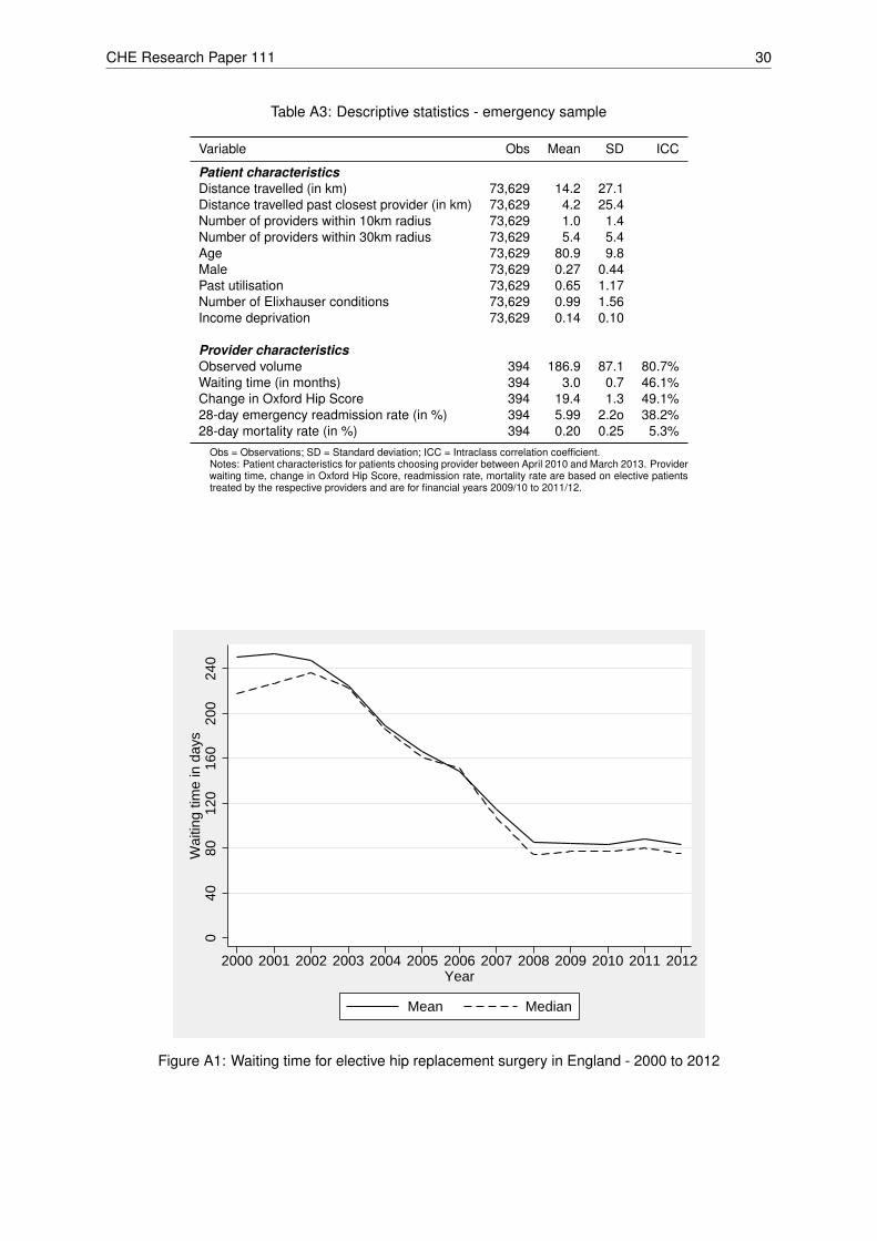
CHE Research Paper 111 30
Table A3: Descriptive statistics - emergency sample
Variable Obs Mean SD ICC
Patient characteristicsDistance travelled (in km) 73,629 14.2 27.1Distance travelled past closest provider (in km) 73,629 4.2 25.4Number of providers within 10km radius 73,629 1.0 1.4Number of providers within 30km radius 73,629 5.4 5.4Age 73,629 80.9 9.8Male 73,629 0.27 0.44Past utilisation 73,629 0.65 1.17Number of Elixhauser conditions 73,629 0.99 1.56Income deprivation 73,629 0.14 0.10
Provider characteristicsObserved volume 394 186.9 87.1 80.7%Waiting time (in months) 394 3.0 0.7 46.1%Change in Oxford Hip Score 394 19.4 1.3 49.1%28-day emergency readmission rate (in %) 394 5.99 2.2o 38.2%28-day mortality rate (in %) 394 0.20 0.25 5.3%
Obs = Observations; SD = Standard deviation; ICC = Intraclass correlation coefficient.Notes: Patient characteristics for patients choosing provider between April 2010 and March 2013. Providerwaiting time, change in Oxford Hip Score, readmission rate, mortality rate are based on elective patientstreated by the respective providers and are for financial years 2009/10 to 2011/12.
040
8012
016
020
024
0W
aitin
g tim
e in
day
s
2000 2001 2002 2003 2004 2005 2006 2007 2008 2009 2010 2011 2012Year
Mean Median
Figure A1: Waiting time for elective hip replacement surgery in England - 2000 to 2012

Do patients choose hospitals that improve their health? 31
80.1
11.0
3.71.3 0.7 0.5 0.4 0.1 0.1 0.1
2.0
0
20
40
60
Per
cent
1 2 3 4 5 6 7 8 9 10 >10
Figure A2: Percentage of emergency patients who went to their Nth nearest hospital