do political incentives matter for tax policies? ideology, opportunism

Do political incentives matter for tax policies?

Ideology, opportunism and the tax structure

by

Konstantinos Angelopoulosa, George Economidesb, Pantelis Kammasc

a Department of Economics, University of Glasgow, Adam Smith Building, Glasgow G12 8RT, United Kingdom. Tel.: +44 (0) 141 330 5273; Fax: +44 (0) 141 330 4940. Email: [email protected]

b Department of International and European Economic Studies, Athens University of Economics and Business, 76 Patission street, Athens 104 34, Greece. Email: [email protected]

c Department of Economics, University of Ioannina, P.O. Box 1186, 45110 Ioannina, Greece. Email: [email protected]

February 12, 2009 Abstract: This paper investigates the importance of political ideology and opportunism in the choice of the tax structure. In particular, we examine the effects of cabinet ideology and elections on the distribution of the tax burden across factors of production and consumption for 21 OECD countries over the period 1970-2001 by employing four alternative cabinet ideology measures and by using the methodology of effective tax rates. There is evidence of both opportunistic and partisan effects on tax policies. More precisely, we find that left-wing governments rely more on capital relative to labor income taxation and that they tend to increase consumption taxes. Moreover, we find that income tax rates (but not consumption taxes) tend to be reduced in pre-electoral periods and that capital effective tax rates (defined broadly to include taxes on self-employed income) are reduced by more than effective labor tax rates. JEL: H1, H2 Keywords: tax structure, political economy, partisan and opportunistic effects

1

1. Introduction

Theoretical and empirical research in political economy has linked policy making to

electoral (opportunistic) and ideological (partisan) incentives (see e.g. Drazen, 2000,

Persson and Tabellini, 2000 and Mueller, 2003) for reviews of this literature).

Opportunistic motives reflect the incumbent party’s desire to win the elections and stay in

office for as long as possible, while the partisan motives arise from assuming that voters

have different preferences (e.g. over public goods), which leads to different policy

platforms adopted by political parties that target the welfare of their constituency.

One strand in this literature has examined the effects of political ideology on the

choice of the tax structure, as defined here by the distribution of the tax burden across

factors of production and consumption (see e.g. the contributions by Persson and

Tabellini, 1992 and 1994, Haufler, 1997 and Lockwood and Markis, 2006 and the survey

paper in Winer and Hettich, 2003). The general conclusion from this body of work is that

left-wing parties would, other things equal, prefer to tax capital income more relative to

labor income, when compared to right-wing parties. Although this is an intuitive

prediction and does conform to anecdotal evidence, we are not aware of an empirical

investigation that examines whether political preferences affect the capital, labor and

consumption tax rates differently.1 We are also not aware of an empirical investigation

that examines whether opportunistic motives affect the capital, labor and consumption tax

rates differently.2 This research is useful both in formally testing the predictions of

theoretical models and in generating stylized facts regarding the political motives behind

the choice of tax rates, with the hope of motivating new theoretical developments.

1 The existing empirical research has mainly examined whether there are partisan effects on the fiscal size of the government (i.e. on fiscal spending as a share of GDP and on the overall tax burden, as the latter is approximated by the share of tax revenue over GDP) and specific fiscal spending and/or tax-revenue categories (see e.g. Alesina, Roubini and Cohen, 1997, Cusack, 1997, Volkerink and de Haan, 2001a, Perotti and Kontopoulos, 2002 and Bräuninger, 2005 for the OECD and Kneebone and McKenzie, 2001 for Canadian provinces). Regarding empirical work on ideology effects on tax rates, we note the study on local property statutory tax rates for Dutch municipalities by Allers et al. (2001) and on the implicit income tax rate in the U.S. states by Reed (2006). Although the work by Reed (2006) is the closest to ours, we note that he does not examine differential effects on labor and capital income and does not consider opportunistic effects. Finally, Tavares (2004) and Mierau et al. (2007) suggest that political variables also matter for fiscal policy adjustment decisions. 2 Note that the standard political business cycle literature (see e.g. the work by Nordhaus, 1975, Linbeck, 1976 and Rogoff, 1990) implies that the incumbent party has the incentive to decrease the tax burden before elections, so as to increase the probability of being re-elected. However, the – theoretical and empirical – literature has not examined the potentially different effects on the different tax rates.

2

Motivated by the above, in this paper we examine the importance of political

ideology and opportunism in the choice of the tax structure. We use the standard

measures of political ideology as in the aforementioned literature. In particular, we use

measures of cabinet orientation developed and used by Castles and Mair (1984), Budge et

al (1993), Cusack (1997), Woldendorp et al. (1998) and Tavares (2004) that are based on

expert surveys and locate parties on an ideological left-right scale. We capture electoral

effects as in the literature, by constructing pre-electoral dummies. In order to approximate

the tax rates on labor income, capital income and consumption we use the ECFIN

effective tax rates reported in Martinez-Mongay (2000). These are based on the Mendoza

et al (1994) approach, which basically consists of defining the tax rate as a ratio between

the tax revenues from a particular tax base and the corresponding tax base. This is

important, because the government is able to affect that tax rates by determining -

through tax legislation – both the statutory tax rate and the tax base differentially for each

source to be taxed. These effective tax rates have not been used so far in the relevant

literature (see however Reed, 2006, who constructs an “implicit” income tax rate for the

U.S. states). Our dataset consists of a panel of 21 OECD countries over the period 1970-

2001. We use the annual data but we also look at 5-year averages, as institutional and

political barriers may make it difficult for policy makers to immediately implement their

policy preferences.

Our main finding is that there exists evidence for effects of both political ideology

and pre-electoral opportunism on the income tax rates for the OECD economies. In

particular, left-wing governments tax capital more relative to labor income. In addition,

governments reduce the income tax rates before elections. These findings are generally

robust to the measures of political ideology used, to the measures of effective tax rates

used and to the use of annual or 5-year averaged data. Importantly, these findings are

consistent with a large body of theoretical research in political economy, as discussed

above. However, these theoretical predictions had not so far received empirical support,

as the data on effective average tax rates that we use here had not been exploited in the

past by the relevant empirical literature.

Equally importantly, using effective tax rates to capture the tax burden on the

factors of production and consumption also reveal some further interesting political

effects. First, it seems that the role of the income of the self employed is important in

examining the effects of ideology on the tax rates. In particular, it is the income of

3

employed labor that the left-wing governments mainly try to reduce relative to income

from capital and self employment. This finding is expected, as long as left-wing parties

view income from self employment as income from entrepreneurial activity and not labor

income. Secondly, we find that the partisan effects are easier to uncover when looking at

the “gross” capital tax rates, although this finding is less robust. Such a result suggests

that left-wing governments increase the tax burden on capital by essentially broadening

the capital tax base, as implied by not being as willing to provide tax exemptions for

depreciated capital. Both findings discussed above underlie the usefulness of using

effective tax rates, as they can capture political effects on both the statutory tax rates and

the tax base and carefully distinguish between different tax bases.

Thirdly, it seems that it is in the capital income (especially when it includes the

income of the self employed) that the reduction in taxation is bigger in pre-electoral

periods. This is not straightforward to explain, based at least on the current theoretical

literature, but it might indicate an increase in lobbying activities in the form of increased

tax avoidance/evasion from the firms in pre-electoral periods, as labor (wage) income

provides fewer opportunities for tax evasion. Fourthly, we find that although income tax

rates are reduced in pre-electoral periods, consumption taxes are not, possibly indicating

that the political cost of the latter is smaller. Finally, we uncover an empirical regularity

that appears puzzling, at least when viewed in the context of the current theoretical

research. In particular, left-wing governments are associated with increases in the

consumption taxes. Explanations to this finding can potentially be obtained by looking at

the relationship between political ideology and the government budget as a whole, which

is an issue we do not examine in this paper.

The rest of the paper is organized as follows. Section 2 presents the data and the

empirical methodology. Section 3 investigates the link between ideological motives and

tax structure. Section 4 investigates the link between electoral motives and tax structure.

Section 5 concludes.

2. Data and empirical methodology

2.1 Tax rates

An important issue in our empirical study of the determinants of the tax structure (and

one that distinguishes this work from related research in the literature) is how to

4

approximate the tax rates. The simple measures of statutory tax rates cannot capture the

complexity of the tax system nor provide a clear indicator of the implied tax policy. Since

the overall tax burden does not depend solely on the statutory tax rates, but also on what

is defined - by the tax legislation - as the tax base, we are in need of some more

complicated tax measures that take into account changes in the tax base (e.g. changes in

allowances or deductions). The approach of calculating average effective tax ratios, based

on the Mendoza et al (1994) approach, basically consists of defining the tax rate as a ratio

between the tax revenues from a particular tax base and the corresponding tax base (for a

critical comparison of alternative effective tax rate methodologies, see Volkerink and de

Haan 2001b). Hence, the main advantage of the average effective tax ratios is exactly that

they carefully define the tax base from which the tax revenue is extracted and hence

provide a more accurate description of the tax burden that falls on each factor input. Tax

revenue as a share of GDP fails to capture the potentially different burdens across factors

of production, or indeed, consumption, as again it is not looking at the correct tax base.

Therefore, effective tax rates are a better proxy for policy changes on the tax structure,

because the government is able to affect that tax rates by determining - through tax

legislation – both the statutory tax rate and the tax base differentially for each source to

be taxed.

Previous empirical studies that examined the effect of partisan ideology and/or

electoral opportunism on tax policies have employed tax revenue as a share of GDP as

dependent variable (see e.g. Alesina et al., 1997, Perotti and Kontopoulos 2002;

Kneebone and McKenzie 2001) or statutory tax rates (e.g. Allers et al., 2001). However,

as discussed above, tax revenue data and statutory tax rates are not adequate proxies of

the tax burden as compared to more sophisticated measures like effective average tax

rates. As far as we know, effective tax rates have not been used so far in empirical

analysis of political effects of tax policy. An exception is Reed (2006) who looks at tax

revenue over personal income in U.S. states, but does not break down this implicit tax

rate in capital, labor income and consumption tax rates. Therefore, previous studies have

not examined the effect of ideology on the distribution of the tax burden across factors of

production and consumption, which we have defined here as the tax structure. Ashworth

and Heyndels (2002) have examined the effect of political incentives on the tax structure,

5

but they approximate the latter by a tax structure turbulence indicator.3 Hence, in this

paper, we make use of the advantages of the effective average tax rates to examine the

effects of political incentives on the tax structure.

In particular, we use the ECFIN effective tax rates reported in Martinez-Mongay

(2000) (see the Appendix for more details on these data), which are available for 21

OECD countries for the 1970-2000 period.4 We use the effective tax rates on labor

(denoted as litr and letr), the effective tax rates on capital (kitn, kitg, ketn and ketg) and

the effective tax rate on consumption (citr and cetr). The difference between the

classification in litr and kitn or kitg compared to letr and ketn or ketg is that in the latter

case, the income of self employed in treated as labor income, whereas in the former case

the labor income includes only the income of employed labor. The difference between

kitn and ketn, compared to kitg and ketg is that in the latter case capital depreciation is

included in the tax base. We shall use the above tax rates to examine whether they are

influenced by political variables, but we shall also consider the ratios of labor to capital

tax rates to try to gauge the potential political effects on the relative income tax burden.

In particular, we construct the variables ratio1, ratio2, ratio3 and ratio4, obtained as

lirt/kitn, lirt/kitg, lert/ketn and lert/ketg respectively.

2.2 Political data

The measurement of differences in policy positions of parties has attracted extensive

attention in the literature (see e.g. Budge, 2001). In the present study we rely on four

alternative party family categorization measures that have been widely employed in order

to analyze the impact of partisan politics on public policy and finance (see e.g. Tavares

2004; Volkerink and de Haan 2001a; Mierau et al 2007). All of these measures are based

on expert surveys that locate parties on an ideological left-right scale (see e.g. Castles and

Mair, 1984; Budge et al. 1993; Woldendorp et al. 1998).

More precisely, we employ: (i) the Budge et al (1993) cabinet ideology index as

updated by Woldendorp et al. (1998) (denoted as ideowold), (ii) the Tavares (2004) 3 The index for tax structure turbulence measures the extent to which country i’s tax structure in a year differs from the tax structure in the pervious year. In order to calculate this tax structure turbulence indicator Ashworth and Heyndels (2002) employ data of tax revenues as a share of GDP which are grouped to six main categories (i.e. taxes on income, profits and capital gains, social security contributions, taxes on payroll and workforce, taxes on goods and services, taxes on property and other taxes). 4 The countries in our sample are: Australia, Austria, Belgium, Canada, Denmark, Finland, France, Germany, Greece, Ireland, Italy, Japan, Luxembourg, Netherlands, Norway, Portugal, Spain, Sweden, Switzerland, UK, USA.

6

cabinet ideology measure (denoted as ideotav), (iii) the Castles and Mair (1984) cabinet

ideology measure (ideocm) and (iv) the cabinet ideology measure developed by Cusack

(1997) (ideocus).5 Both Woldendorp et al. (1998) and Tavares (2004) cabinet ideology

indices locate cabinet ideology on a 1 to 5 political spectrum with higher values denoting

more extreme left-wing governments. On the other hand, Cusack (1997) and Castles and

Mair (1984) measures locate government ideology on a min-max range with higher

values denoting more extreme right-wing government.6

Finally, opportunistic effects are captured by a dummy variable (denoted as

elections) which equals one in years in which a national election was held and zero in

non-elections years. Data for elections are obtained by Cusack (1997).

2.3 Empirical methodology

We wish to estimate the effects of political ideology and opportunism on the tax

structure, in a panel of 21 OECD countries observed over 1970-2000. In order to examine

the effects of ideology on the tax structure, we mainly focus on 5-year periods and

calculate data averages for the six 5-year periods between 1970 and 2000.7 The reason for

preferring 5-year periods to annual data to analyze the effects of ideology on policy

decisions is that institutional and political barriers may make it difficult for policy makers

to immediately implement their policy preferences. In working with 5-year averages we

follow the relevant literature (see e.g. Reed, 2006). However, as a robustness check, we

also use the annual data as such. In order to examine electoral effects on tax-policy

choices, we focus on the annual data, as this is in accordance with the natural timing of

elections and also the usual approach in the related literature (see e.g. Kneebone and

McKenzie, 2001).

5 It is worth noting that these alternative cabinet ideology measures are based on two broad party family classifications. The first one is that developed by Budge et al. (1993) and followed by Woldendorp et al (1998) and Tavares (2004) whereas the second is that of Castles and Mair (1984) also followed by Cusack (1997). Thus, we expect ideowold to be more related to ideotav and ideocm to ideocus. 6 Castles and Mair (1984) generate their ideological scores from a questionnaire survey of more than 115 political scientists in Western Europe and United States. Each expert was asked to place parties holding seats in the national legislature on a left-wing political spectrum ranging from 0 (extreme left-wing) to 10 (extreme right-wing, with 2.5, 5 and 7.5 representing moderate left, the center and moderate right, respectively. Cusack (1997) developed his measure of cabinet ideology based on the Castles and Mair ideological scores. Ideocus is coded on a 1 to 5 scale with higher values denoting more extreme right-wing governments. 7 The averages are calculated for the 5-year periods 1971-1975, 1976-1980, 1981-1985, 1986-1990, 1991-1995 and 1996-2000.

7

We define the tax structure as the distribution of the tax burden across factors of

production and consumption. In order to examine the effect of political factors in the

choice of the tax structure, we look at the effect of political ideology and pre-election

motives at the levels of the labor, capital and consumption tax rates, using the political

and tax data described above. Focusing on the allocation of the tax burden between the

labor and capital production inputs, which has attracted most of the interest in the

theoretical literature, we also examine the effect of the political variables on the ratio of

labor to capital tax rates. The advantage of this approach is that it looks at the relative

burden. For instance, left-wing governments might prefer to increase both tax rates on

capital and labor, relative to right-wing governments, so that by looking at the ideology

effects on levels might not easily reveal a preference for left-wing governments to

increase the tax burden on capital relative to labor. However, looking at the ratio of the

tax rates, we could capture such ideology effects on the tax structure.

The equations we estimate are of the form:

ititititit uXpoltaxtax ++++= − βααα 2110 (1)

where ittax is the measure of tax rate or of the ratio of labor to capital tax rates of country

i at time period t ( t being the 5-year period or the year), itpol is a measure of political

ideology or pre-electoral motives, and itX includes control variables usually included in

regressions for fiscal policy measures (see below). Note that the regression includes the

lagged value of the ittax measure, to account for persistence in tax policies. We also

allow for country and time specific effects, so that the error term is written as:

ittiit vcu ε++= (2)

where itε is assumed to be i.i.d. In what follows, we control for country effects by either

fixed effects estimation or by first differencing. We also control for time effects by

including dummies for each time period in our regressions.

Our interest here lies in estimating 2α , the effect of political variables. We assume

throughout this analysis, following the literature, that measures of political ideology and

8

opportunism are exogenous in estimating models of the form of (1) – (2). However,

dynamic panel data models as the above do not satisfy the strict exogeneity assumption,

because of the presence of the lagged dependent variable as a regressor. In addition,

certain variables in itX may only be predetermined or even endogenous in (1) – (2) (see

e.g. Baltagi, 2001, ch. 8 and Wooldridge, 2002, ch. 11, on panel data models without the

strict exogeneity assumption). Ignoring the above, generally results in biases in the

estimated coefficients.

It can be shown (see e.g. the references above) that the size of the inconsistency

introduced by the fixed effects estimator when strict exogeneity is not satisfied decreases

by the time dimension of the panel. Therefore, as fiscal and political data are in general

available for many years for many countries, the literature (see the papers referred to

above) has used this result to estimate equations like (1) – (2) by fixed effects. Here,

when we use the annual data, the same arguments apply, as we have data for 26-29 time

periods, depending on the political variables and tax measures we use. Therefore, for the

annual dataset we present results from fixed effects estimation (this has the additional

advantage of making our results more easily comparable to those of the relevant

literature). However, for the dataset in 5-year averages, we have data for 4 time periods

only, when we take into account the requirements of lagging the data and taking first

differences. Hence, for this dataset, we explicitly allow for predetermined variables in (1)

– (2) and present results by using the Arellano and Bond (1991) GMM estimator.8

Regarding the variables included in itX we follow the literature on the

determinants of national tax structure (see e.g. Devereux et al. 2007, 2008; Winner,

2005).9 The literature is generally looking at determinants of the overall size of the

government or of proxies for the level of the tax rates. In this study, we run regressions

for the level of the tax rates, but we also look at the tax structure, as measured by the ratio

of labor to capital tax rates. This has not been examined in the literature. Hence, for these

regressions, existing research does not help to create a clear expectation for the effect of

the variables in itX on the dependent variable.

8 We also report that estimating the equations for the 5-year dataset with fixed effects and the equations for the annual dataset with GMM as in Arellano and Bond (1991), does not change the main qualitative results discussed below, regarding the coefficients of the key variables of interest - the political measures. 9 More details on the data used are in the Data Appendix.

9

We first include in itX the GDP per capita (denoted as gdppc). This is obtained

from the World Bank Development Indicators (2004) (hereafter WDI (2004)) and for the

5-year period dataset it is the value of the year before the 5-period (i.e. for the period

1981-1985 it is the value of 1980), while it is the value of the previous year for the annual

dataset. According to Wagner’ law, we would expect gdppc to be positively related with

measures of the overall size of the government, but there is no ex ante theoretical reason

for a positive or negative relationship with measures of the tax structure. As a country

gets richer, it may need to rely more or less on labor versus capital taxation or on direct

versus indirect taxation. An additional economic variable that can be related with the tax

structure is the level of government spending. Government spending is expected to be

positively related with taxation, but again higher government spending may require more

or less labor versus capital taxation or direct versus indirect taxation. To control for the

effects of government spending on the tax structure, we present results using government

expenditure as a share of GDP, available from WDI, denoted as govexp and averaged

over the 5-year periods for the dataset in 5-year averages.10

We also include some standard demographic variables: the proportion of the

economically dependent population (denoted as agedep), the total population

(population) and the urbanization rate (denoted as urban) (i.e. the proportion of

population living in urban areas). Data for these variables are obtained from WDI (2004).

Agedep is expected to be positively related with taxation since higher proportion of

economically dependent population generate fiscal needs which in turn increase tax rates.

However, there is no clear theoretical reason for a positive or negative relation with the

ratios of labor to capital tax rates. On the other hand, population and urban are expected

to be negatively related with taxation. This is because these measures capture potential

economies of scales in the provision of public goods (Alesina and Wacziarg, 1998).

Larger economies of scale induce lower per capita cost of public goods and consequently

lower levels of taxation. Again, there is no ex ante theoretical reason for a positive or

negative relationship with measures of the tax structure. Finally, we employ the capital

market international integration measure constructed by Quinn (1997) (denoted as

10 This is the total expenditure of the central government (see the Data Appendix for more details). We report that the basic results do not change if we use total expenditures of the general government, available from GFS. In fact, the z-statistics and t-statistics for the political variables of interest in Tables 1 and 4 get higher and the z-statistics and t-statistics for the capital tax rates in Tables 2 and 5 get also bigger. We present results using the WDI variable (govexp) because there more observations available for this.

10

capopenness). Capopenness is coded on a 0 to 100 scale with higher values denoting

weaker international capital mobility restrictions and thus more integrated capital market.

According to the tax competition theory (see e.g. Bucovetsky and Wilson, 1991)

capopenness is expected to be positively related with labor tax rates and negatively with

capital tax rates.11 We use the 5-year average of these variables for the dataset in 5-year

averages.

3. Ideology and the tax structure

In this section we examine whether the data suggest a relationship between the ideology

of the party in government and tax policy choices. We first present results using 5-year

averages and then present results using the annual dataset.

3.1 Results using 5-year averages for the tax ratios

We first examine whether the ideological orientation of the government matters for the

tax structure, as approximated by the ratio of labor to capital effective tax rates. We

estimate (1) – (2), with the control variables discussed in section 2.3, by using the

Arellano and Bond (1991) GMM estimator, where the lagged dependent variable is

instrumented by all the available lags. In addition, we allow in these regressions for non-

exogeneity of gdppc and govexp. In particular, gdppc may only be predetermined, as

contemporaneous correlation with the error term can be ruled out (since we use the

lagged value of per capita GDP), but strict exogeneity need not hold, because the error

term can be correlated with future values of gdppc. Regarding govexp, we want to allow

for potential endogeneity, as, for instance, governments may react to exogenous negative

shocks by changing both government spending and the allocation of the tax burden.

Hence, in the GMM regressions, we treat gdppc as predetermined and govexp as

endogenous and use lagged values as instruments (we use a maximum of two lagged

values as instruments).

Results for the ratios of the labor to capital tax rates are presented in Table 1.

When we take into account the requirements of lagging the data and taking first

11 According to the benchmark tax competition model (Zodrow and Mieszkowski, 1986) tax competition among different regions leads to suboptimally low capital tax rates and an inefficiently low level of public goods. Allowing for a second tax instrument (i.e. a labor tax), the local governments find it optimal to rely more on labor taxation to finance the public good (Bucovetsky and Wilson, 1991).

11

differences, the sample period for estimation is the four 5-year periods in 1980-2000.

Time dummies are included for each period in all equations. Two specification tests are

also reported. The 2m statistic, proposed by Arellano and Bond (1991) to test for second

order serial correlation in the residuals of the first-differenced equations and the Sargan

test statistic of over-identifying restrictions, to test for the validity of the instruments.

[Table 1 here]

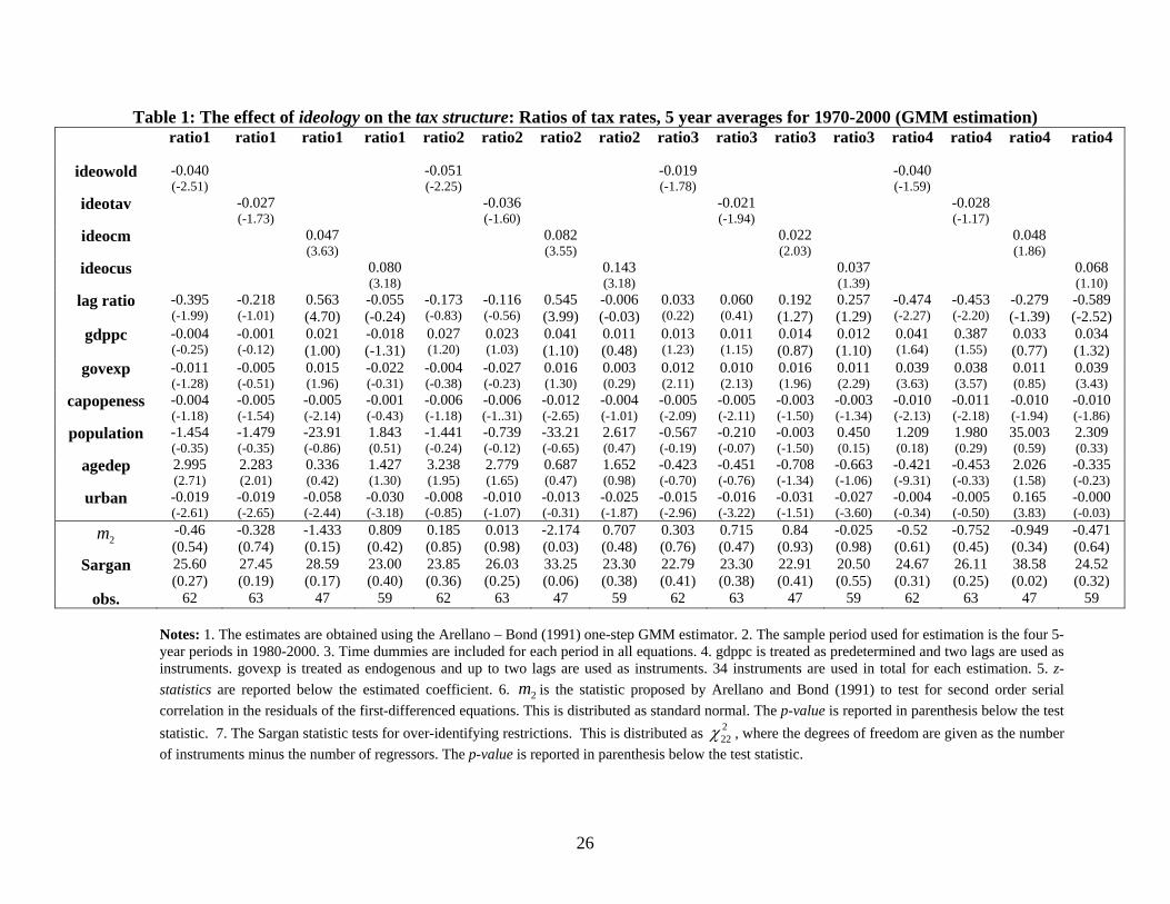
Table 1 presents the results for the effects of the four measures of political

ideology on the four labor-to-capital tax ratios. In all cases, the coefficients of the

political variables indicate similar qualitative results. Namely, left-wing governments

tend to rely more on capital taxation relative to labor taxation. More precisely, the

coefficient of ideowold bears a negative sign and is statistically significant, at least for the

three first ratios (for the fourth ratio it is marginally insignificant at 10% level). Similar

results, regarding the sign, are obtained also for the coefficient of ideotav, which appears

to be statistically significant for the first and the third ratio. The coefficient on ideocm

bears a positive sign and is statistically significant for all four ratios, whereas the

coefficient on ideocus is positive and is statistically significant for the first two ratios.

Note that the implications of ideocm and ideocus are similar to the ones of the previous

measures (ideowold and ideotav), since the positive sign of these coefficients is simply

due to the opposite way that ideocm and ideocus classify left-wing and right wing

cabinets relative to ideowold and ideotav (see Section 2.2 for details).

Our first result is therefore that left-wing governments increase the taxation of

capital, relative to that on labor. It is interesting to note that this result is more robust

when we look at ratio1 and ratio2. In addition, note that the estimated coefficients are

generally bigger for the regressions for ratio1 and ratio2 compared to those for ratio3

and ratio4. Recall that in the first two ratios the numerator is litr. As explained above, the

difference between litr and letr (the numerator in ratio3 and ratio4) is that the income of

the self-employed is not treated as labor income in litr. Hence, the data suggest that left-

wing political ideology is likely to decrease the tax burden on the income of employed

labor relative to income from capital and self employment.

Regarding the explanatory variables, the coefficients of govexp and agedep are

positive when they are statistically significant, whereas capopenness and urban enter

12

with negative and statistically significant coefficients in some cases. Moreover, we

observe that gdppc and population are insignificant in all the estimations. As we have

already pointed out, there are not clear theoretical predictions regarding the estimates for

the control variables in the regressions where the dependent variables are ratios of labor

to capital tax rates.12 In any case, the results seem to suggest that when governments are

faced with budgetary pressures, in the form of increased expenditure or adverse

demographic evolutions, they tend to increase labor taxes more than capital taxes. In

addition, the negative sign obtained for the coefficient of urban could indicate that in

more urbanized societies, workers have more lobbying power on governmental decisions.

However, this interpretation is not robust as we shall see below. Finally, we observe that

the estimated coefficients of the lagged ratios change sign across regressions with

different dependent variables, but also across regressions with different political

determinants, for the same dependent variable. Hence, although there seems to be

persistence in the choice of the tax system, there is no robust pattern across different tax

ratios.

Concerning the specification tests, there are two cases in Table 1, for the

regressions using the ideocm measure for ratio2 and ratio4, where the specification tests

reject the nulls, but the overall picture is good with – generally – high p-values.

3.2 Results using 5-year averages for the level of tax rates

Table 1 shows that left-wing governments prefer a lower ratio of labor to capital taxation

than right wing governments. But is this realized by decreases in the labor tax rate or

increases in the capital tax rate? A lower labor to capital ratio can also be obtained if the

government increases both taxes, but increase capital taxation by more relative to labor;

or, if the government decreases both taxes, but decreases capital taxation by less relative

to labor. We now try to answer this question.

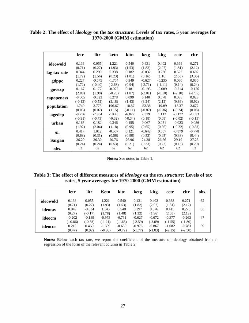
[Tables 2 and 3 here]

12 An exception is capopenness. As we have already noted, according to the tax competition theory this capital market integration measure would be expected to be positively related with the ratio of labor to capital tax rates. However, our empirical findings suggest a negative relationship between capopenness and most of the labor to capital tax ratios. This puzzling result, which is mainly driven by the positive effect of capopenness on the levels of capital tax rates (see Table 2), will be discussed below with the results of Table 2.

13

In Tables 2 and 3 we present results from regressions where the levels of the

effective average tax rates are regressed on the political measures and the control

variables described before, using the Arellano and Bond (1991) GMM estimator, as for

the regressions in Table 1. In Table 2, we present the results for the regressions where

ideowold is the political variable, whereas in Table 3, to save on space, we only report the

estimated coefficients of political variables obtained from similar regressions where these

variables are used as a measure of ideology.

Three basic results emerge. First, there seems to be no effect of ideology on the

labor tax rates, as all four alternative ideology proxies are not significant in the

regressions where litr and letr are the dependent variables. Although this could indeed

indicate that there are no ideology effects on the level of the labor income tax rates, we

need to be careful as partisan motives may work in labor income taxation through the

progressivity of the tax system, which the effective average tax rates fail to capture.

Secondly, more left-wing governments tend to increase the tax burden on capital.

This result is clear in the cases of the “gross” rates (i.e. where kitg and ketg are the

dependent variables) but also holds in some of the estimations where ketn and kitn are the

dependent variables. The finding that partisan effects are easier to uncover when looking

at the “gross” capital tax rates is interesting as it highlights the advantages of looking at

the effects of ideology on both the statutory tax rates and the tax base, as indeed captured

by the effective tax rates. In particular, the above results suggest that left-wing

governments increase the tax burden on capital by essentially broadening the capital tax

base. The latter takes place as left-wing governments are not being as willing to provide

tax exemptions for depreciated capital.

Finally, there is clear evidence that left-wing governments tend to also increase

consumption taxes. In most the regressions where citr and cetr are the dependent

variables, political ideology measures bear statistically significant coefficients. This is an

interesting and somewhat puzzling finding, as one might expect that right-wing

governments would prefer to tax consumption more than left-wing governments, given

that consumption taxation is regressive with respect to income. One potential explanation

for our finding here is that left-wing parties are likelier to prefer a larger government, but

note that government expenditure has a negative sign in these regressions, once ideology

is controlled for. Another potential explanation would be that left-wing governments

might prefer to use the consumption tax income to decrease accumulated debt, whereas

14

right-wing governments might be more willing to live with larger debts (see e.g. Alesina

and Tabellini (1990) and Lockwood et al. (1996) for the role of ideology on public debt

accumulation). A careful examination of political ideology on the dynamics of the

government budget could provide useful empirical findings regarding the robustness and

explanation of this relationship, but this is beyond the scope of this paper.

Regarding the control variables, gdppc is insignificant in most regressions, while

govexp is positive and statistically significant in the regressions where litr and letr are the

dependent variables but is negative in most of the remaining regressions, indicating that

increases in fiscal spending are financed primarily by increases in labor income

taxation.13 Population and agedep are not significant, whereas capopenness enters with

positive sign in most of the regressions where capital tax rates are the dependent variable.

The puzzling positive relationship between capopenness and capital tax rates could be

attributed to the “tax cut cum base broadening” strategy followed by most of the OECD

economies as a response to international market integration.14 In any case, this result is

not robust to using the annual data, as we shall see below.

We also present, in Table 2, the specification tests we presented in Table 1; they

are all supportive of the model specification. We report that similar results are generally

obtained for the regressions in Table 3.15

3.3 Results using the annual dataset

In this sub-section, we examine the robustness of the previous results when we use the

annual data. Therefore, we re-estimate the equations in (1)-(2), using the annual data 13 We note that these results are not robust (see Table 5 and Table7) and thus we do not proceed further with this. The same (non-robustness) applies to the estimated positive effect of urban in the regressions with the labor tax rates. 14 Although in most OECD countries statutory tax rates on capital have fallen sharply over the past few decades, the tax bases have been broadened through reduced allowances and deductions. Tax reforms have followed the so-called “tax cut cum base broadening” strategy, leaving the effective tax rate on capital fairly stable or even increasing. This “tax cut cum base broadening” strategy can be best explained by focusing on the operation of multinational enterprises (MNE), and especially on the practice of profit shifting among the subsidiary and its parent. This practice –followed by MNE-of transferring part of taxable profits in countries with low statutory tax rates has led national governments to compete for (paper) profits by lowering their statutory tax rates. This downward trend of statutory tax rates has been accompanied by a corresponding broadening of the tax base (though reduced allowances and deductions), which left the corporate effective tax rates fairly stable or even increasing. For two excellent surveys on corporate income tax reforms in OECD countries see Devereux et. al. (2002) and Griffith and Klemm (2004). 15 The p-values for the serial correlation and the Sargan tests are in general high for all the regressions in Table 3, with the exception of the Sargan statistic for the ideocus regression for letr, where the p-value is approximately 10%, and the serial correlation statistic for the ideocm regression for letr, where the p-value is at 9%.

15

from 1970 to 2000. In order to account for country-specific and time-specific

unobservable factors we introduce country and time dummies in all equations. Results for

the ratios of the labor to capital tax rates are presented in Table 4, while results for the

levels of the tax rates are in Tables 5 and 6.

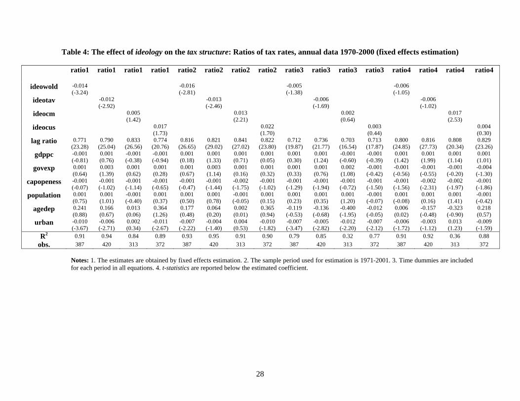
[Table 4 here]

Table 4 presents the results for the effects of the four measures of political

ideology on the four labor to capital tax ratios. As can be seen, our empirical findings

remain qualitative intact although deteriorate in terms of statistical significance, mainly

for ratio3 and ratio4, which is again consistent with our previous speculation that left-

wing governments target primarily the income of employed labor. Note also that the

estimated coefficients are twice as big or bigger for the regressions for ratio1 and ratio2

compared to those for ratio3 and ratio4.

Generally, as before, the coefficients of all four alternative political variables

indicate that left-wing governments tend to rely more on capital relative to labor taxation.

More precisely, the coefficient of ideowold bears a negative and statistically significant

for ratio1 and ratio2 whereas appears to be marginally insignificant for ratio3. Similar

results, regarding the sign, are obtained also for the coefficient of ideotav which appears

to be statistically significant for the first three ratios. Ideocm enters with a positive and

statistically significant coefficient in the cases of ratio2 and ratio4, whereas the

coefficient on ideocus is positive and is statistically significant for the first two ratios.

Concerning the explanatory variables, our results are qualitative similar to those

presented in Table 1 regarding the coefficients of capopenness and urban. In particular,

they remain negative, although capopenness is not significant in most regressions. The

coefficients of govexp and agedep are not significant. It is worth noting that, as expected,

there is much more persistence in the annual tax rates, as is verified by the high

coefficients and t-ratios for the lagged dependent variables in Table 4.

[Tables 5 and 6 here]

In Tables 5 and 6 we present results from regressions where the levels of the effective

average tax rates are regressed on the political measures and the control variables

16

described before, using the two-way error component fixed effect estimator and the

annual dataset, as for the regressions in Table 4. More precisely, in Table 5, we present

the results for the regressions where ideowold is the political variable, whereas in Table

6, to save on space, we report the estimated coefficient of all four political variables

obtained from similar regressions.

Generally, the results are consistent with those presented in the previous section.

In particular, none of the coefficients of the political variables measures appears to be

significant in regressions where litr or letr are the dependent variables. This implies that

there seems to be no effect of ideology on the effective average labor tax rates. On the

other hand, in most of the estimations where capital tax rates are the dependent variables,

the political ideology proxies suggest that left-wing governments tend to increase the tax

burden on capital. Nevertheless, the t-ratios for the political ideology coefficients are

generally lower compared to Table 3, which explains the lower t-ratios for the political

ideology coefficients in Table 4. Finally there is again clear evidence that left-wing

governments tend also to rely on indirect taxation. In all the estimations where citr and

cetr are the dependent variables, the political ideology measures enter with highly

significant coefficients.

Regarding the control variables our results remain qualitative similar. Gdppc, and

govexp are positive in those regressions where they are statistically significant, whereas

capopenness, population and agedep are not insignificant. Urban is now significant in the

regressions for the capital tax rates, which is consistent with its negative sign in Tables 1

and 4. Finally, the lagged level of the tax rates is always highly significant.

4. Electoral cycles and the tax structure

In this section we examine whether the data indicate electoral effects on tax policy

choices. The literature has documented a negative effect of pre-electoral periods on

taxation (see e.g. Kneebone and Mc Kenzie, 2001) which is consistent with the

implications of the theoretical literature of political business cycles, i.e. that incumbent

policy makers try to decrease that tax burden before elections in an effort to increase their

probability for re-election (see e.g. Nordhaus, 1975, Linbeck, 1976 and Rogoff, 1990). It

is important, however, to examine whether labor or capital taxes decrease more in pre-

electoral periods.

17

We present results using the annual dataset and, following the literature, we use a

dummy for pre-election periods to capture electoral motives. We use the same set of

control variables described above. Again, given the long time series dimension of the

panel, we estimate our equations by fixed effects. Results are reported in Table 7. For

each dependent variable in this Table, we run two regressions, one that includes a

political ideology variable (ideowold) in addition to the electoral dummy, and one where

the only political variable is the electoral dummy.

[Table 7 here]

We first look at the levels of the effective tax rates, where the presence of

opportunistic effects on tax policy is strikingly apparent. The coefficient of the election

dummy is negative and highly significant in the regressions where litr and letr are the

dependent variable indicating that governments tend to reduce the tax burden on labor in

pre-electoral periods. Similar effects are verified also in most of the cases where capital

tax rates are employed as dependents. In particular, election enters with a negative and

statistically significant coefficient in the regressions where kitn, kitg and ketg are

dependent variables highlighting the negative effect of electoral uncertainty on the tax

burden on capital. However, the presence of opportunistic effects is not clear in the

regressions where consumption taxes are employed as dependent variables. In particular,

the estimated coefficients for elections are in this case only marginally significant and

very sensitive to the inclusion of the political ideology proxy.

The above results suggest that the governments tend to decrease the income tax

rates before elections, but not necessarily the consumption tax rates. This implies that the

income tax rates (are perceived to) have a bigger impact on voters’ choices compared to

consumption taxes. Although such an explanation seems intuitive, we are not aware of

theoretical research that would support such a prediction.

To further investigate the effects of electoral opportunism on the income tax rates,

we examine whether there is evidence to suggest that governments reduce labor or capital

tax rates by more before elections. As can be seen in Table 7, elections enter with a

positive and statistically significant coefficient in the estimations where ratio1 and ratio2

are the dependent variables once we control for partisan effects. This result suggests that

although in pre-electoral periods both the tax burdens on labor and capital are reduced,

18

the ratio of the tax rates on capital fall by more, at least when we control for ideology

effects on the relative tax rates (this is also confirmed when we look at the coefficients of

elections in the regressions for kitn and kitg versus litr). Recall also that the numerator in

ratio1 and ratio2 is the tax rate on employed labor. This implies that the reduction in the

labor to capital taxes in pre-electoral periods is clearer when we include the income of the

self-employed in the capital taxes. Therefore, it seems that in pre-electoral periods not

only the capital tax rates but (primarily) the tax revenue collected from the self employed

is reduced. Given that capital income and the income from self employment is the most

difficult to tax, our findings here are consistent with increased tax avoidance/evasion in

pre-electoral periods (see also Angelopoulos and Economides, 2008, for a theoretical

model and empirical evidence that rent seeking activities related to the government

budget increase in pre-electoral periods).

5. Conclusions

We examined the effects of political ideology and pre-electoral opportunism on the tax

rates and found that there is evidence of both for the OECD economies. In particular, our

main finding regarding the income tax rates is that left-wing governments tax capital

more relative to labor income and that governments reduce the income tax rates before

elections. Although these findings are consistent with the theoretical research in political

economy, they had not so far received empirical support, as the data on effective average

tax rates that we use here had not been exploited in the past by the relevant empirical

literature.

Equally importantly, using effective tax rates to capture the tax burden on the

factors of production and consumption has also revealed some further interesting political

effects. First, it seems that the role of the income of the self employed is important in

examining the effects of ideology on the tax rates. In particular, it is the income of

employed labor that the left-wing governments mainly try to reduce relative to income

from capital and self employment. This finding is expected, as long as left-wing parties

view income from self employment as income from entrepreneurial activity and not labor

income. Secondly, we found that the partisan effects are easier to uncover when looking

at the “gross” capital tax rates, although this finding is less robust. Such a result suggests

that left-wing governments increase the tax burden on capital by essentially broadening

19

the capital tax base, as implied by not being as willing to provide tax exemptions for

depreciated capital. Both findings discussed above underlie the usefulness of using

effective tax rates, as they can capture political effects on both the statutory tax rates and

the tax base and carefully distinguish between different tax bases.

Thirdly, it seems that it is in the capital income (especially when it includes the

income of the self employed) that the reduction in taxation is bigger in pre-electoral

periods. This is not straightforward to explain, based at least on the current theoretical

literature, but it might indicate an increase in lobbying activities in the form of increased

tax avoidance/evasion from the firms in pre-electoral periods, as labor (wage) income

provides fewer opportunities for tax evasion. Fourthly, we found that although income

tax rates are reduced in pre-electoral periods, consumption taxes are not, possibly

indicating that the political cost of the latter is smaller. Finally, we uncovered an

empirical regularity that appears puzzling, at least when viewed in the context of the

current theoretical research. In particular, left-wing governments are associated with

increases in the consumption taxes. We believe that explanations to this finding can be

obtained by looking at the relationship between political ideology and the government

budget as a whole, which we leave as future research.

A limitation of working with effective average tax rates is that we cannot capture

ideology effects on the progressivity of the tax system. Provided that adequate measures

of tax progressivity can be constructed, it would be interesting to examine whether such

effects exist. In addition, it would be a useful addition to the empirical literature on the

political determinants of fiscal policy to examine the effects of ideology and opportunism

on the composition of government spending and the government budget more generally.

20

References Alesina, A., Cohen, G., Roubini, N., 1992. Macroeconomic policy and elections in OECD democracies. Economics and Politics, 4, 1-30. Alesina, A., Roubini, N., 1992. Political cycles in OECD economies. Review of Economic Studies, 59, 663-688. Alesina A., Roubini N., Cohen G., 1997. Political Cycles and the Macroeconomy, The MIT Press, Cambridge, Mass. Alesina, A., Tabellini, G., 1990. A positive theory of fiscal deficits and government debt. Review of Economic Studies, 57, 403-414. Alesina, A., Wacziarg, R., 1998. Openness, country size and government. Journal of Public Economics, 69, 305-321 Allers, M., de Haan, J., Sterks, C., 2001. Partisan influence on the local tax burden in the Netherlands. Public Choice, 106, 351-363. Angelopoulos, K., Economides, G., 2008. Fiscal policy, rent seeking and growth under electoral uncertainty: theory and evidence from the OECD, Canadian Journal of Economics, 41(4), 1375-1405. Ashworth, J., Heyndels, B., 2002. Tax structure turbulence in OECD countries. Public Choice, 111, 374-376. Bräuninger, T., 2005. A Partisan Model of Government Expenditure. Public Choice, 125, 409-429. Bucovetsky, S., Wilson, J. D., 1991. Tax competition with two tax instruments. Regional Science and Urban Economics, 21, 333–350. Budge, I., Kemam, H., Woldendrop, J., 1993. Political data 1945–90. European Journal of Political Research, Special Issue 24, 1– 120. Castles, F., Mair, P., 1984. Left– right political scales: some expert judgements. European Journal of Political Research, 12, 73– 88. Cusack, T., 1997. Partisan politics and public finance: changes in public spending in the industrialized democracies, 1955-1998. Public Choice, 91, 375-395. Devereux, M., Griffith , R., Klemm, A., 2002. Corporate income tax reform and international tax competition. Economic Policy, 35, 449-488. Devereux, M., Lockwood, B., Redoano, M., 2007. Horizontal and vertical indirect tax competition: Theory and some evidence from the USA. Journal of Public Economics, 91, 451-479.

21

Devereux, M., Lockwood, B., Redoano, M., 2008. Do countries compete over corporate tax rates? Journal of Public Economics, 92, 1210-1235. Drazen, A., 2000. Political Economy in Macroeconomics. Princeton University Press, Princeton, New Jersey.

Griffith, R., Klemm, A., 2004. What has been the tax competition experience of the last 20 years? Tax Notes International, 34, 1299-1316. Haufler, A., 1997. Factor Taxation, Income Distribution and Capital Market Integration. Scandinavian Journal of Economics, 99, 425–446. Kneebone, R., McKenzie, K., 2001. Electoral and partisan cycles in fiscal policy: An examination of Canadian provinces. International Tax and Public Finance, 8, 753-774. Laver, M., Hunt, W.B., 1992. Policy and Party Competition. Routledge, Chapman and Hall, New York. Lindbeck, A., 1976. Stabilization policies in open economies with endogenous politicians. American Economic Review Papers and Proceedings, 66, 1-19. Lockwood, B., Makris, M., 2006. Tax incidence, majority voting and capital market integration, Journal of Public Economics, 90, 1007– 1025. Lockwood, B., Philippopoulos, A., Snell, A., 1996. Fiscal policy, public debt stabilisation and politics: Theory and UK evidence, Economic Journal, 106, 894-911. Martinez-Mongay, C., 2000. ECFIN’s effective tax rates: Properties and comparisons with other tax indicators, Economic Paper no. 146, Brussels: European Commission, Directorate for Economic and Financial Affairs. Mendoza, E., Razin, A., Tesar, L., 1994. Effective tax rates in macroeconomics: cross-country estimates of tax rates on factor income and consumption. Journal of Monetary Economics, 34, 447-461. Mierau, J., Jong-A-Pin, R., de Haan, J., 2007. Do political variables affect fiscal policy adjustment decisions? New empirical evidence. Public Choice, 133, 297-319. Mueller, D., 2003. Public Choice III. Cambridge University Press. Nordhaus, W., 1975. The political business cycle. Review of Economic Studies, 42, 169-190. Perotti, R., Kontopoulos,Y., 2002. Fragmented fiscal policy. Journal of Public Economics, 86, 191-222. Persson, T., Tabellini, G. 1992. The politics of 1992: Fiscal policy and European integration. Review of Economic Studies, 59, 689–701.

22

Persson, T., Tabellini, G., 1994. Representative democracy and capital taxation, Journal of Public Economics, 55, 53-70. Persson, T., Tabellini, G., 2000. Political economics: explaining economic policy. MIT Press. Cambridge Quinn, D., 1997. The correlates of change in international financial regulation. American Political Science Review, 91, 531-551. Reed, R., 2006. Democrats, republicans, and taxes: Evidence that political parties matter. Journal of Public Economics, 90, 725-750. Rogoff, K., 1990. Equilibrium political budget cycles. American Economic Review, 80, 21-36. Tavares, J., 2004. Does right or left matter? Cabinets, credibility and fiscal adjustments. Journal of Public Economics, 88, 2447-2468. Volkerink, B., de Haan, J., 2001a. Fragmented Government Effects on Fiscal Policy: New Evidence. Public Choice, 109, 221-242. Volkerink, B., de Haan, J., 2001b. Tax ratios: a critical survey. OECD Tax Policy Studies, 1-80. Winer, S., L., Hettich, W., 2003. The Political Economy of Taxation: Positive and Normative Analysis when Collective Choice Matters. In C. W. Rowley and F. Schneider (eds.), The Encyclopedia of Public Choice. Dordrecht, Netherlands: Kluwer Academic Publishers. Winner, H., 2005. Has tax competition emerged in OECD countries? Evidence from panel data. International Tax and Public Finance, 12, 667-687. Woldendorp, J., Keman, H., Budge, I., 1998. Party government in 20 democracies: an update (1990–1995). European Journal of Political Research, 33, 125– 164. World Bank. 2004. World Bank Development Indicators, CD-ROM, Washington D.C.: World Bank. Zodrow, G., Mieszkowski, P., 1986. Pigou, Tiebout, property taxation, and the underprovision of local public goods. Journal of Urban Economics, 19, 356–370.

23

Appendices

Appendix A: ECFIN effective tax rates in more detail

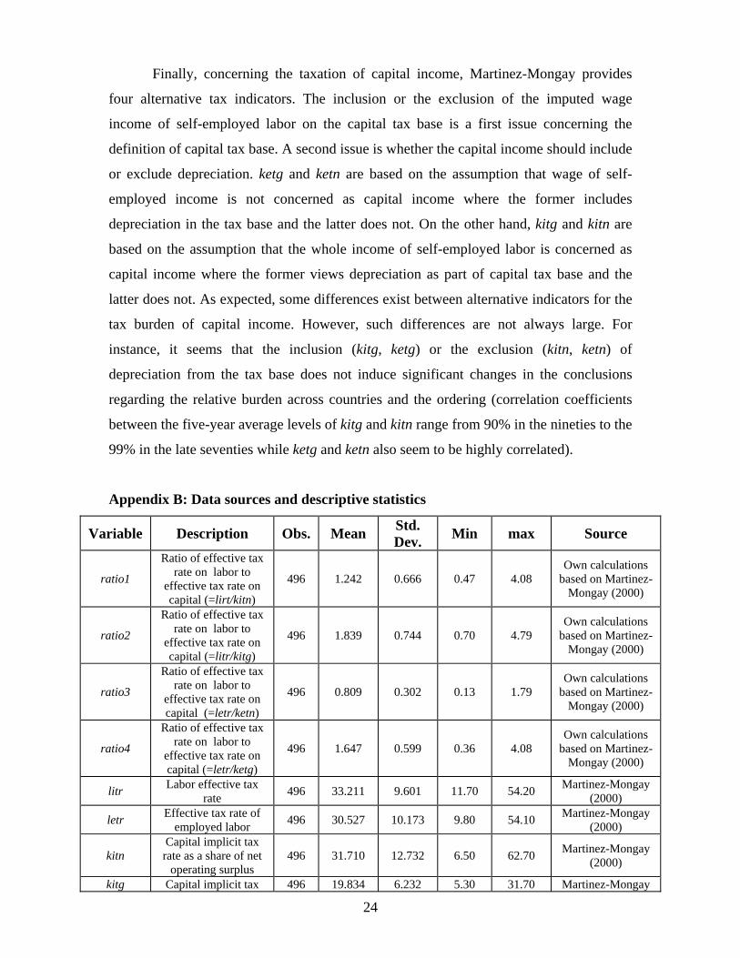
The ECFIN effective tax rates on labor (denoted as litr and letr), on consumption (citr

and cetr) and on capital (kitn, kitg, ketn and ketg) used in this paper are all taken from

Martinez-Mongay (2000). Martinez-Mongay calls litr, citr, kitn and kitg as “implicit” tax

rates and letr, cetr, ketn and ketg as “effective” tax rates.16 All these alternative tax rates

are based on the same principle of “effective taxation”. The methodology of effective tax

rates, following Mendoza et al. (1994), basically consists of defining the tax rate as a

ratio between the tax revenues from particular taxes and the corresponding tax base (for a

critical comparison of different methodologies, see Volkerink and de Haan, 2001b).

Concerning the effective tax rate on labor, Martinez-Mongay provides two

different tax indicators: letr can be viewed as a more general measure of tax on labor

income while litr better proxies the tax burden faced by the employed labor (thus

excludes the taxation of the imputed wage of self-employed labor). Although differences

between the two rates are minor in the case of more advanced economies, there are

countries (e.g. Greece and Portugal) where the two rates differ significantly in terms of

level. This is because in these countries the share of self-employed labor to the total

employment is larger. However, despite divergences in level, the evolution of litr and letr

over time seem to be common (correlation coefficients between the five-year average

levels of litr and letr range from 91% in the nineties to 97% in the late seventies).

Following the general concept of effective tax rates, the effective tax rate on

consumption should be the ratio of tax revenues from consumption taxes to the pre-tax

value of consumption. Thus the effective tax rate on consumption is the difference

between the consumer price (post tax price) and the producer price (pre tax price)

expressed as a percentage of producer price (cetr) or the consumer price (citr). It is clear

form the above that citr and cetr are equivalent in terms of evolution over time or

between countries, although citr is always smaller in terms of level (in the case of the

euro area and EU-15 the difference is of 5 to 6 percentage points). Both correlation

coefficients between the five years average levels of citr and cetr are equal to one (see

Martinez-Mongay, pp.37-38)

16 It is worth noting that the letr, citr, and ketg variables are closer to the standard Mendoza et al. (1994) methodology of effective tax rates.

24

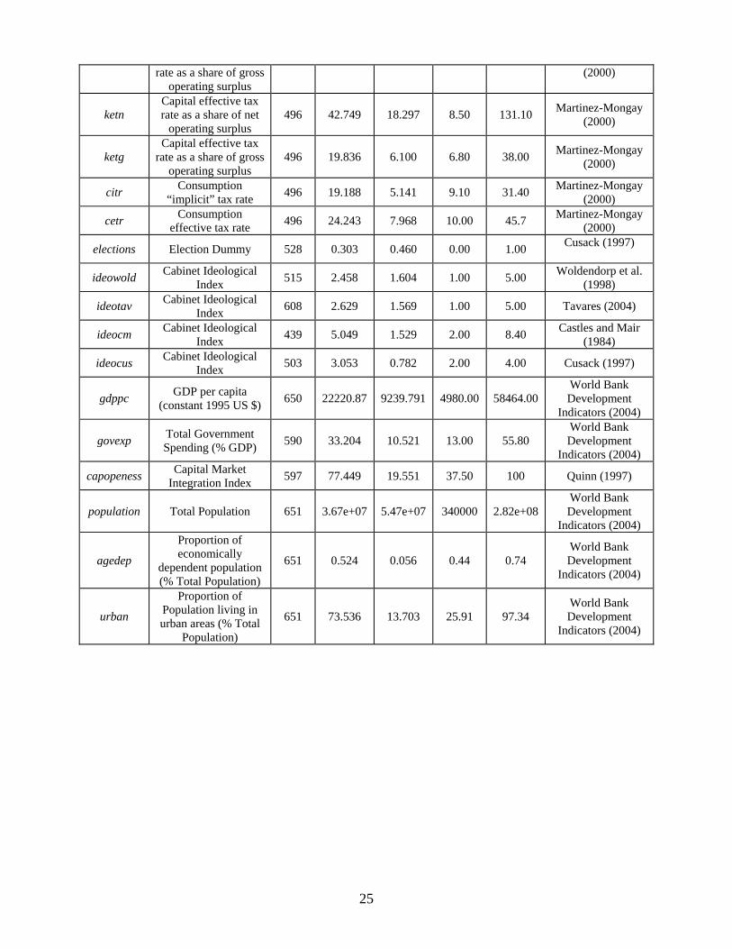
Finally, concerning the taxation of capital income, Martinez-Mongay provides

four alternative tax indicators. The inclusion or the exclusion of the imputed wage

income of self-employed labor on the capital tax base is a first issue concerning the

definition of capital tax base. A second issue is whether the capital income should include

or exclude depreciation. ketg and ketn are based on the assumption that wage of self-

employed income is not concerned as capital income where the former includes

depreciation in the tax base and the latter does not. On the other hand, kitg and kitn are

based on the assumption that the whole income of self-employed labor is concerned as

capital income where the former views depreciation as part of capital tax base and the

latter does not. As expected, some differences exist between alternative indicators for the

tax burden of capital income. However, such differences are not always large. For

instance, it seems that the inclusion (kitg, ketg) or the exclusion (kitn, ketn) of

depreciation from the tax base does not induce significant changes in the conclusions

regarding the relative burden across countries and the ordering (correlation coefficients

between the five-year average levels of kitg and kitn range from 90% in the nineties to the

99% in the late seventies while ketg and ketn also seem to be highly correlated).

Appendix B: Data sources and descriptive statistics

Variable Description Obs. Mean Std. Dev. Min max Source

ratio1

Ratio of effective tax rate on labor to

effective tax rate on capital (=lirt/kitn)

496 1.242 0.666 0.47 4.08 Own calculations

based on Martinez-Mongay (2000)

ratio2


effective tax rate on capital (=litr/kitg)



ratio3


effective tax rate on capital (=letr/ketn)



ratio4


effective tax rate on capital (=letr/ketg)



litr Labor effective tax rate 496 33.211 9.601 11.70 54.20 Martinez-Mongay

(2000)

letr Effective tax rate of employed labor 496 30.527 10.173 9.80 54.10 Martinez-Mongay

(2000)

kitn Capital implicit tax rate as a share of net

operating surplus 496 31.710 12.732 6.50 62.70 Martinez-Mongay

(2000)

kitg Capital implicit tax 496 19.834 6.232 5.30 31.70 Martinez-Mongay

25

rate as a share of gross operating surplus

(2000)

ketn Capital effective tax rate as a share of net

operating surplus 496 42.749 18.297 8.50 131.10 Martinez-Mongay

(2000)

ketg Capital effective tax

rate as a share of gross operating surplus

496 19.836 6.100 6.80 38.00 Martinez-Mongay (2000)

citr Consumption “implicit” tax rate 496 19.188 5.141 9.10 31.40 Martinez-Mongay

(2000)

cetr Consumption effective tax rate 496 24.243 7.968 10.00 45.7 Martinez-Mongay

(2000)

elections Election Dummy 528 0.303 0.460 0.00 1.00 Cusack (1997)

ideowold Cabinet Ideological Index 515 2.458 1.604 1.00 5.00 Woldendorp et al.

(1998)

ideotav Cabinet Ideological Index 608 2.629 1.569 1.00 5.00 Tavares (2004)

ideocm Cabinet Ideological Index 439 5.049 1.529 2.00 8.40 Castles and Mair

(1984)

ideocus Cabinet Ideological Index 503 3.053 0.782 2.00 4.00 Cusack (1997)

gdppc GDP per capita (constant 1995 US $) 650 22220.87 9239.791 4980.00 58464.00

World Bank Development

Indicators (2004)

govexp Total Government Spending (% GDP) 590 33.204 10.521 13.00 55.80

World Bank Development

Indicators (2004)

capopeness Capital Market Integration Index 597 77.449 19.551 37.50 100 Quinn (1997)

population Total Population 651 3.67e+07 5.47e+07 340000 2.82e+08 World Bank Development

Indicators (2004)

agedep

Proportion of economically

dependent population (% Total Population)

651 0.524 0.056 0.44 0.74 World Bank Development

Indicators (2004)

urban

Proportion of Population living in urban areas (% Total

Population)

651 73.536 13.703 25.91 97.34 World Bank Development

Indicators (2004)

26

Table 1: The effect of ideology on the tax structure: Ratios of tax rates, 5 year averages for 1970-2000 (GMM estimation)

ratio1 ratio1 ratio1 ratio1 ratio2 ratio2 ratio2 ratio2 ratio3 ratio3 ratio3 ratio3 ratio4 ratio4 ratio4 ratio4

ideowold -0.040 (-2.51)

-0.051 (-2.25)

-0.019 (-1.78)

-0.040 (-1.59)

ideotav -0.027 (-1.73)

-0.036 (-1.60)

-0.021 (-1.94)

-0.028 (-1.17)

ideocm 0.047 (3.63)

0.082 (3.55)

0.022 (2.03)

0.048 (1.86)

ideocus 0.080 (3.18)

0.143 (3.18)

0.037 (1.39)

0.068 (1.10)

lag ratio -0.395 (-1.99)

-0.218 (-1.01)

0.563 (4.70)

-0.055 (-0.24)

-0.173 (-0.83)

-0.116 (-0.56)

0.545 (3.99)

-0.006 (-0.03)

0.033 (0.22)

0.060 (0.41)

0.192 (1.27)

0.257 (1.29)

-0.474 (-2.27)

-0.453 (-2.20)

-0.279 (-1.39)

-0.589 (-2.52)

gdppc -0.004 (-0.25)

-0.001 (-0.12)

0.021 (1.00)

-0.018 (-1.31)

0.027 (1.20)

0.023 (1.03)

0.041 (1.10)

0.011 (0.48)

0.013 (1.23)

0.011 (1.15)

0.014 (0.87)

0.012 (1.10)

0.041 (1.64)

0.387 (1.55)

0.033 (0.77)

0.034 (1.32)

govexp -0.011 (-1.28)

-0.005 (-0.51)

0.015 (1.96)

-0.022 (-0.31)

-0.004 (-0.38)

-0.027 (-0.23)

0.016 (1.30)

0.003 (0.29)

0.012 (2.11)

0.010 (2.13)

0.016 (1.96)

0.011 (2.29)

0.039 (3.63)

0.038 (3.57)

0.011 (0.85)

0.039 (3.43)

capopeness -0.004 (-1.18)

-0.005 (-1.54)

-0.005 (-2.14)

-0.001 (-0.43)

-0.006 (-1.18)

-0.006 (-1..31)

-0.012 (-2.65)

-0.004 (-1.01)

-0.005 (-2.09)

-0.005 (-2.11)

-0.003 (-1.50)

-0.003 (-1.34)

-0.010 (-2.13)

-0.011 (-2.18)

-0.010 (-1.94)

-0.010 (-1.86)

population -1.454 (-0.35)

-1.479 (-0.35)

-23.91 (-0.86)

1.843 (0.51)

-1.441 (-0.24)

-0.739 (-0.12)

-33.21 (-0.65)

2.617 (0.47)

-0.567 (-0.19)

-0.210 (-0.07)

-0.003 (-1.50)

0.450 (0.15)

1.209 (0.18)

1.980 (0.29)

35.003 (0.59)

2.309 (0.33)

agedep 2.995 (2.71)

2.283 (2.01)

0.336 (0.42)

1.427 (1.30)

3.238 (1.95)

2.779 (1.65)

0.687 (0.47)

1.652 (0.98)

-0.423 (-0.70)

-0.451 (-0.76)

-0.708 (-1.34)

-0.663 (-1.06)

-0.421 (-9.31)

-0.453 (-0.33)

2.026 (1.58)

-0.335 (-0.23)

urban -0.019 (-2.61)

-0.019 (-2.65)

-0.058 (-2.44)

-0.030 (-3.18)

-0.008 (-0.85)

-0.010 (-1.07)

-0.013 (-0.31)

-0.025 (-1.87)

-0.015 (-2.96)

-0.016 (-3.22)

-0.031 (-1.51)

-0.027 (-3.60)

-0.004 (-0.34)

-0.005 (-0.50)

0.165 (3.83)

-0.000 (-0.03)

2m -0.46 (0.54)

-0.328 (0.74)

-1.433 (0.15)

0.809 (0.42)

0.185 (0.85)

0.013 (0.98)

-2.174 (0.03)

0.707 (0.48)

0.303 (0.76)

0.715 (0.47)

0.84 (0.93)

-0.025 (0.98)

-0.52 (0.61)

-0.752 (0.45)

-0.949 (0.34)

-0.471 (0.64)

Sargan 25.60 (0.27)

27.45 (0.19)

28.59 (0.17)

23.00 (0.40)

23.85 (0.36)

26.03 (0.25)

33.25 (0.06)

23.30 (0.38)

22.79 (0.41)

23.30 (0.38)

22.91 (0.41)

20.50 (0.55)

24.67 (0.31)

26.11 (0.25)

38.58 (0.02)

24.52 (0.32)

obs. 62 63 47 59 62 63 47 59 62 63 47 59 62 63 47 59 Notes: 1. The estimates are obtained using the Arellano – Bond (1991) one-step GMM estimator. 2. The sample period used for estimation is the four 5-year periods in 1980-2000. 3. Time dummies are included for each period in all equations. 4. gdppc is treated as predetermined and two lags are used as instruments. govexp is treated as endogenous and up to two lags are used as instruments. 34 instruments are used in total for each estimation. 5. z-statistics are reported below the estimated coefficient. 6. 2m is the statistic proposed by Arellano and Bond (1991) to test for second order serial correlation in the residuals of the first-differenced equations. This is distributed as standard normal. The p-value is reported in parenthesis below the test statistic. 7. The Sargan statistic tests for over-identifying restrictions. This is distributed as 2

22χ , where the degrees of freedom are given as the number of instruments minus the number of regressors. The p-value is reported in parenthesis below the test statistic.

27

Table 2: The effect of ideology on the tax structure: Levels of tax rates, 5 year averages for 1970-2000 (GMM estimation)

letr litr ketn kitn ketg kitg cetr citr

ideowold 0.133 (0.71)

0.055 (0.27)

1.221 (1.93)

0.540 (1.53)

0.431 (1.82)

0.402 (2.07)

0.368 (1.81)

0.271 (2.12)

lag tax rate 0.344 (1.72)

0.299 (1.56)

0.338 (0.23)

0.182 (1.01)

-0.032 (0.16)

0.236 (1.16)

0.523 (2.55)

0.692 (3.35)

gdppc 0.227 (1.72)

-0.075 (-0.40)

-1.704 (-2.63)

0.349 (0.94)

-0.627 (-2.71)

-0.235 (-1.11)

0.030 (0.14)

0.036 (0.24)

govexp 0.167 (2.00)

0.177 (1.98)

-0.075 (-0.28)

0.181 (1.07)

-0.195 (-2.01)

-0.009 (-0.10)

-0.214 (-2.10)

-0.126 (-1.95)


-0.023 (-0.52)

0.278 (2.18)

0.099 (1.43)

0.140 (3.24)

0.078 (2.12)

0.035 (0.86)

0.023 (0.92)

population 1.740 (0.03)

3.775 (0.07)

196.67 (1.15)

-10.87 (-0.11)

-52.38 (-0.87)

-19.09 (-0.36)

-13.37 (-0.24)

2.672 (0.08)

agedep -9.256 (-0.91)

-7.904 (-0.73)

-10.45 (-0.32)

-6.827 (-0.34)

2.329 (0.18)

1.112 (0.08)

-0.172 (-0.02)

-1.033 (-0.15)

urban 0.165 (1.92)

0.182 (2.04)

0.346 (1.18)

0.155 (0.95)

0.067 (0.65)

0.051 (0.56)

-0.023 (-0.22)

-0.056 (-0.83)

2m 0.417 (0.68)

1.012 (0.31)

-0.587 (0.56)

0.121 (0.90)

-0.642 (0.52)

0.067 (0.95)

-0.879 (0.38)

-0.778 (0.44)

Sargan 26.20 (0.24)

26.30 (0.24)

20.76 (0.53)

26.96 (0.21)

24.38 (0.33)

26.66 (0.22)

29.19 (0.13)

27.23 (0.20)

obs. 62 62 62 62 62 62 62 62

Notes: See notes in Table 1.

Table 3: The effect of different measures of ideology on the tax structure: Levels of tax rates, 5 year averages for 1970-2000 (GMM estimation)

letr litr Ketn kitn ketg kitg cetr citr obs.

ideowold 0.133 (0.71)

0.055 (0.27)

1.221 (1.93)

0.540 (1.53)

0.431 (1.82)

0.402 (2.07)

0.368 (1.81)

0.271 (2.12)

62

ideotav 0.049 (0.27)

-0.034 (-0.17)

1.143 (1.78)

0.548 (1.48)

0.297 (1.32)

0.376 (1.96)

0.415 (2.05)

0.270 (2.13)

63

ideocm -0.202 (--0.86)

-0.139 (-0.58)

-0.973 (-1.21)

-0.731 (-1.65)

-0.627 (-2.59)

-0.672 (-3.09)

-0.377 (-1.55)

-0.263 (-1.80)

47

ideocus 0.219 (0.47)

0.460 (0.92)

-1.609 (-0.98)

-0.650 (-0.72)

-0.976 (-1.77)

-0.867 (-1.83)

-1.082 (-2.15)

-0.783 (-2.50)

59

Notes: Below each tax rate, we report the coefficient of the measure of ideology obtained from a regression of the form of the relevant column in Table 2.

28

Table 4: The effect of ideology on the tax structure: Ratios of tax rates, annual data 1970-2000 (fixed effects estimation)

ratio1 ratio1 ratio1 ratio1 ratio2 ratio2 ratio2 ratio2 ratio3 ratio3 ratio3 ratio3 ratio4 ratio4 ratio4 ratio4

ideowold -0.014 (-3.24)

-0.016 (-2.81)

-0.005 (-1.38)

-0.006 (-1.05)

ideotav -0.012 (-2.92)

-0.013 (-2.46)

-0.006 (-1.69)

-0.006 (-1.02)

ideocm 0.005 (1.42)

0.013 (2.21)

0.002 (0.64)

0.017 (2.53)

ideocus 0.017 (1.73)

0.022 (1.70)

0.003 (0.44)

0.004 (0.30)

lag ratio 0.771 (23.28)

0.790 (25.04)

0.833 (26.56)

0.774 (20.76)

0.816 (26.65)

0.821 (29.02)

0.841 (27.02)

0.822 (23.80)

0.712 (19.87)

0.736 (21.77)

0.703 (16.54)

0.713 (17.87)

0.800 (24.85)

0.816 (27.73)

0.808 (20.34)

0.829 (23.26)

gdppc -0.001 (-0.81)

0.001 (0.76)

-0.001 (-0.38)

-0.001 (-0.94)

0.001 (0.18)

0.001 (1.33)

0.001 (0.71)

0.001 (0.05)

0.001 (0.30)

0.001 (1.24)

-0.001 (-0.60)

-0.001 (-0.39)

0.001 (1.42)

0.001 (1.99)

0.001 (1.14)

0.001 (1.01)

govexp 0.001 (0.64)

0.003 (1.39)

0.001 (0.62)

0.001 (0.28)

0.001 (0.67)

0.003 (1.14)

0.001 (0.16)

0.001 (0.32)

0.001 (0.33)

0.001 (0.76)

0.002 (1.08)

-0.001 (-0.42)

-0.001 (-0.56)

-0.001 (-0.55)

-0.001 (-0.20)

-0.004 (-1.30)


-0.001 (-1.02)

-0.001 (-1.14)

-0.001 (-0.65)

-0.001 (-0.47)

-0.001 (-1.44)

-0.002 (-1.75)

-0.001 (-1.02)

-0.001 (-1.29)

-0.001 (-1.94)

-0.001 (-0.72)

-0.001 (-1.50)

-0.001 (-1.56)

-0.002 (-2.31)

-0.002 (-1.97)

-0.001 (-1.86)

population 0.001 (0.75)

0.001 (1.01)

-0.001 (-0.40)

0.001 (0.37)

0.001 (0.50)

0.001 (0.78)

-0.001 (-0.05)

0.001 (0.15)

0.001 (0.23)

0.001 (0.35)

0.001 (1.20)

-0.001 (-0.07)

0.001 (-0.08)

0.001 (0.16)

0.001 (1.41)

-0.001 (-0.42)

agedep 0.241 (0.88)

0.166 (0.67)

0.013 (0.06)

0.364 (1.26)

0.177 (0.48)

0.064 (0.20)

0.002 (0.01)

0.365 (0.94)

-0.119 (-0.53)

-0.136 (-0.68)

-0.400 (-1.95)

-0.012 (-0.05)

0.006 (0.02)

-0.157 (-0.48)

-0.323 (-0.90)

0.218 (0.57)

urban -0.010 (-3.67)

-0.006 (-2.71)

0.002 (0.34)

-0.011 (-2.67)

-0.007 (-2.22)

-0.004 (-1.40)

0.004 (0.53)

-0.010 (-1.82)

-0.007 (-3.47)

-0.005 (-2.82)

-0.012 (-2.20)

-0.007 (-2.12)

-0.006 (-1.72)

-0.003 (-1.12)

0.013 (1.23)

-0.009 (-1.59)

R2 0.91 0.94 0.84 0.89 0.93 0.95 0.91 0.90 0.79 0.85 0.32 0.77 0.91 0.92 0.36 0.88 obs. 387 420 313 372 387 420 313 372 387 420 313 372 387 420 313 372

Notes: 1. The estimates are obtained by fixed effects estimation. 2. The sample period used for estimation is 1971-2001. 3. Time dummies are included for each period in all equations. 4. t-statistics are reported below the estimated coefficient.

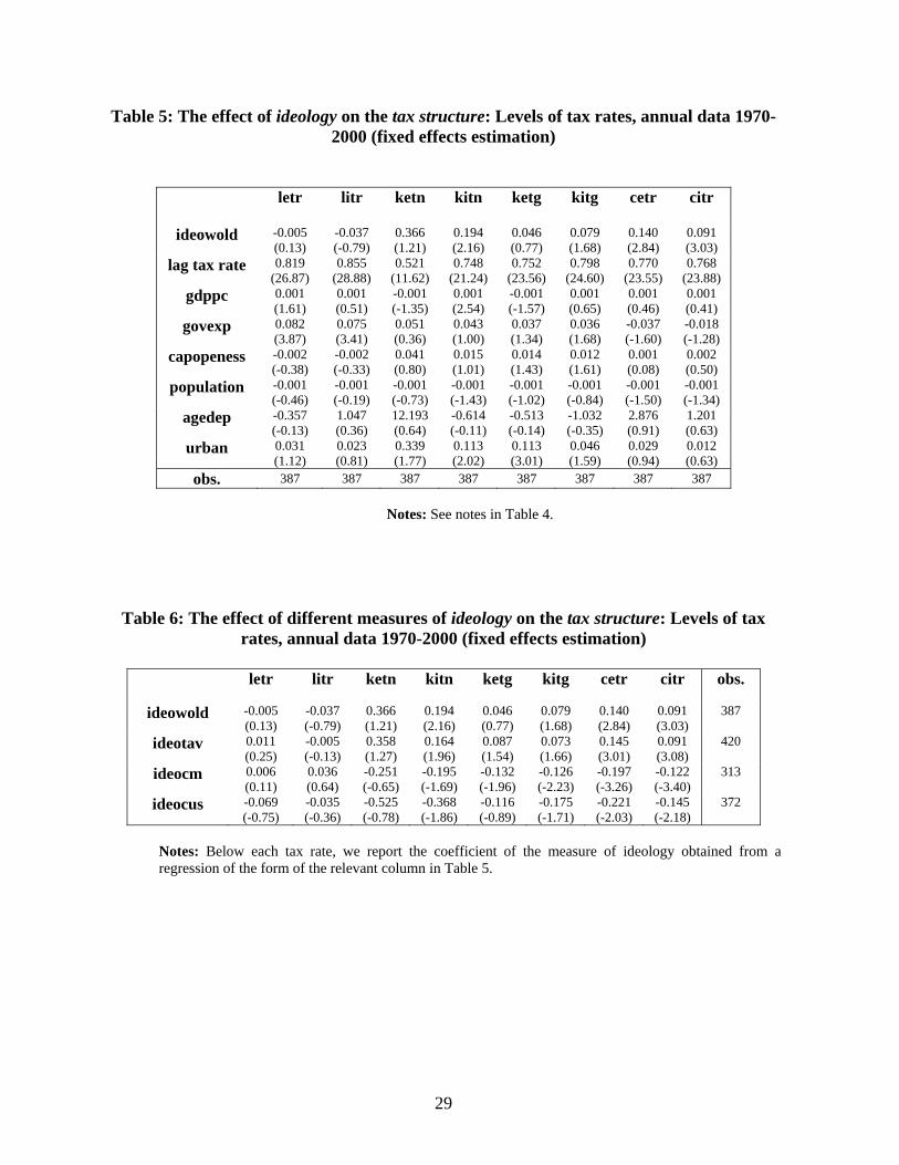
29

Table 5: The effect of ideology on the tax structure: Levels of tax rates, annual data 1970-2000 (fixed effects estimation)

letr litr ketn kitn ketg kitg cetr citr

ideowold -0.005 (0.13)

-0.037 (-0.79)

0.366 (1.21)

0.194 (2.16)

0.046 (0.77)

0.079 (1.68)

0.140 (2.84)

0.091 (3.03)

lag tax rate 0.819 (26.87)

0.855 (28.88)

0.521 (11.62)

0.748 (21.24)

0.752 (23.56)

0.798 (24.60)

0.770 (23.55)

0.768 (23.88)

gdppc 0.001 (1.61)

0.001 (0.51)

-0.001 (-1.35)

0.001 (2.54)

-0.001 (-1.57)

0.001 (0.65)

0.001 (0.46)

0.001 (0.41)

govexp 0.082 (3.87)

0.075 (3.41)

0.051 (0.36)

0.043 (1.00)

0.037 (1.34)

0.036 (1.68)

-0.037 (-1.60)

-0.018 (-1.28)


-0.002 (-0.33)

0.041 (0.80)

0.015 (1.01)

0.014 (1.43)

0.012 (1.61)

0.001 (0.08)

0.002 (0.50)

population -0.001 (-0.46)

-0.001 (-0.19)

-0.001 (-0.73)

-0.001 (-1.43)

-0.001 (-1.02)

-0.001 (-0.84)

-0.001 (-1.50)

-0.001 (-1.34)

agedep -0.357 (-0.13)

1.047 (0.36)

12.193 (0.64)

-0.614 (-0.11)

-0.513 (-0.14)

-1.032 (-0.35)

2.876 (0.91)

1.201 (0.63)

urban 0.031 (1.12)

0.023 (0.81)

0.339 (1.77)

0.113 (2.02)

0.113 (3.01)

0.046 (1.59)

0.029 (0.94)

0.012 (0.63)

obs. 387 387 387 387 387 387 387 387

Notes: See notes in Table 4.

Table 6: The effect of different measures of ideology on the tax structure: Levels of tax rates, annual data 1970-2000 (fixed effects estimation)

letr litr ketn kitn ketg kitg cetr citr obs.

ideowold -0.005 (0.13)

-0.037 (-0.79)

0.366 (1.21)

0.194 (2.16)

0.046 (0.77)

0.079 (1.68)

0.140 (2.84)

0.091 (3.03)

387

ideotav 0.011 (0.25)

-0.005 (-0.13)

0.358 (1.27)

0.164 (1.96)

0.087 (1.54)

0.073 (1.66)

0.145 (3.01)

0.091 (3.08)

420

ideocm 0.006 (0.11)

0.036 (0.64)

-0.251 (-0.65)

-0.195 (-1.69)

-0.132 (-1.96)

-0.126 (-2.23)

-0.197 (-3.26)

-0.122 (-3.40)

313

ideocus -0.069 (-0.75)

-0.035 (-0.36)

-0.525 (-0.78)

-0.368 (-1.86)

-0.116 (-0.89)

-0.175 (-1.71)

-0.221 (-2.03)

-0.145 (-2.18)

372

Notes: Below each tax rate, we report the coefficient of the measure of ideology obtained from a regression of the form of the relevant column in Table 5.

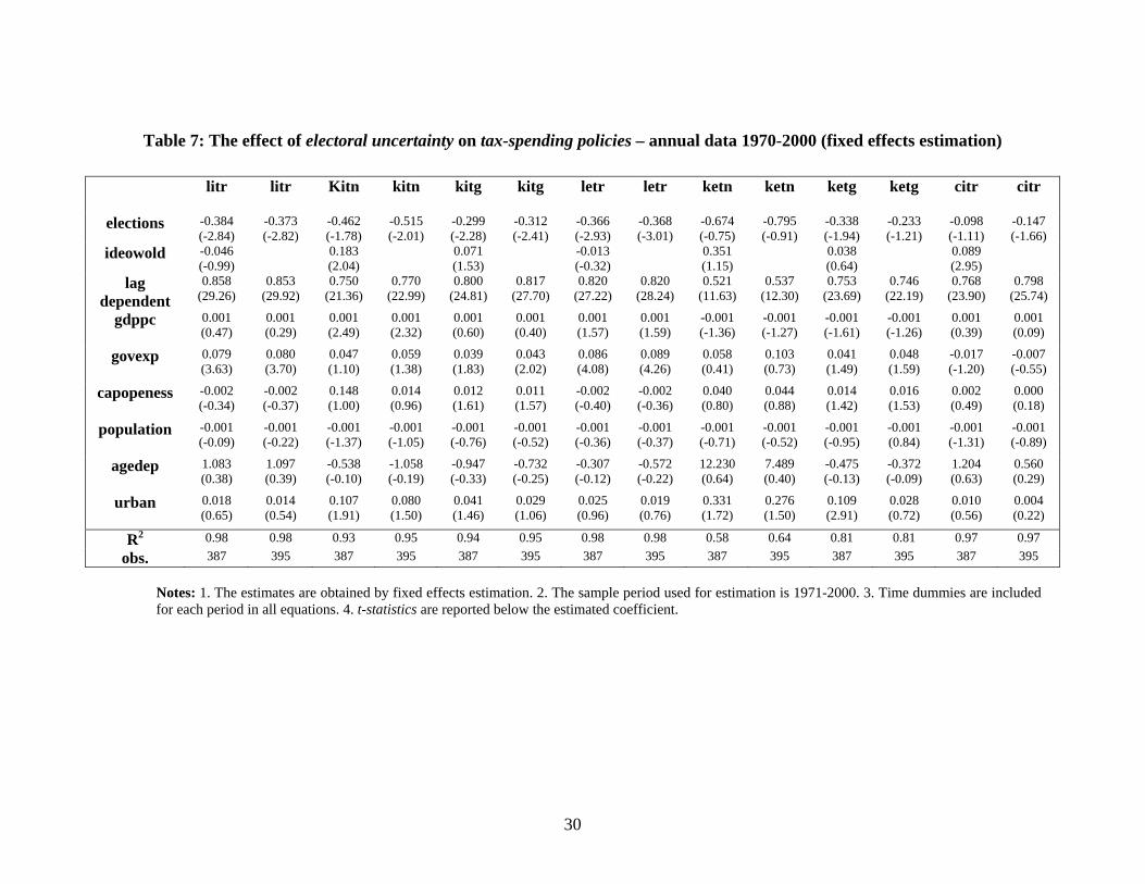
30

Table 7: The effect of electoral uncertainty on tax-spending policies – annual data 1970-2000 (fixed effects estimation)

Notes: 1. The estimates are obtained by fixed effects estimation. 2. The sample period used for estimation is 1971-2000. 3. Time dummies are included for each period in all equations. 4. t-statistics are reported below the estimated coefficient.

litr litr Kitn kitn kitg kitg letr letr ketn ketn ketg ketg citr citr

elections -0.384 (-2.84)

-0.373 (-2.82)

-0.462 (-1.78)

-0.515 (-2.01)

-0.299 (-2.28)

-0.312 (-2.41)

-0.366 (-2.93)

-0.368 (-3.01)

-0.674 (-0.75)

-0.795 (-0.91)

-0.338 (-1.94)

-0.233 (-1.21)

-0.098 (-1.11)

-0.147 (-1.66)

ideowold -0.046 (-0.99)

0.183 (2.04)

0.071 (1.53)

-0.013 (-0.32)

0.351 (1.15)

0.038 (0.64)

0.089 (2.95)

lag dependent

0.858 (29.26)

0.853 (29.92)

0.750 (21.36)

0.770 (22.99)

0.800 (24.81)

0.817 (27.70)

0.820 (27.22)

0.820 (28.24)

0.521 (11.63)

0.537 (12.30)

0.753 (23.69)

0.746 (22.19)

0.768 (23.90)

0.798 (25.74)

gdppc

0.001 (0.47)

0.001 (0.29)

0.001 (2.49)

0.001 (2.32)

0.001 (0.60)

0.001 (0.40)

0.001 (1.57)

0.001 (1.59)

-0.001 (-1.36)

-0.001 (-1.27)

-0.001 (-1.61)

-0.001 (-1.26)

0.001 (0.39)

0.001 (0.09)

govexp

0.079 (3.63)

0.080 (3.70)

0.047 (1.10)

0.059 (1.38)

0.039 (1.83)

0.043 (2.02)

0.086 (4.08)

0.089 (4.26)

0.058 (0.41)

0.103 (0.73)

0.041 (1.49)

0.048 (1.59)

-0.017 (-1.20)

-0.007 (-0.55)

capopeness

-0.002 (-0.34)

-0.002 (-0.37)

0.148 (1.00)

0.014 (0.96)

0.012 (1.61)

0.011 (1.57)

-0.002 (-0.40)

-0.002 (-0.36)

0.040 (0.80)

0.044 (0.88)

0.014 (1.42)

0.016 (1.53)

0.002 (0.49)

0.000 (0.18)

population

-0.001 (-0.09)

-0.001 (-0.22)

-0.001 (-1.37)

-0.001 (-1.05)

-0.001 (-0.76)

-0.001 (-0.52)

-0.001 (-0.36)

-0.001 (-0.37)

-0.001 (-0.71)

-0.001 (-0.52)

-0.001 (-0.95)

-0.001 (0.84)

-0.001 (-1.31)

-0.001 (-0.89)

agedep

1.083 (0.38)

1.097 (0.39)

-0.538 (-0.10)

-1.058 (-0.19)

-0.947 (-0.33)

-0.732 (-0.25)

-0.307 (-0.12)

-0.572 (-0.22)

12.230 (0.64)

7.489 (0.40)

-0.475 (-0.13)

-0.372 (-0.09)

1.204 (0.63)

0.560 (0.29)

urban

0.018 (0.65)

0.014 (0.54)

0.107 (1.91)

0.080 (1.50)

0.041 (1.46)

0.029 (1.06)

0.025 (0.96)

0.019 (0.76)

0.331 (1.72)

0.276 (1.50)

0.109 (2.91)

0.028 (0.72)

0.010 (0.56)

0.004 (0.22)

R2 0.98 0.98 0.93 0.95 0.94 0.95 0.98 0.98 0.58 0.64 0.81 0.81 0.97 0.97 obs. 387 395 387 395 387 395 387 395 387 395 387 395 387 395

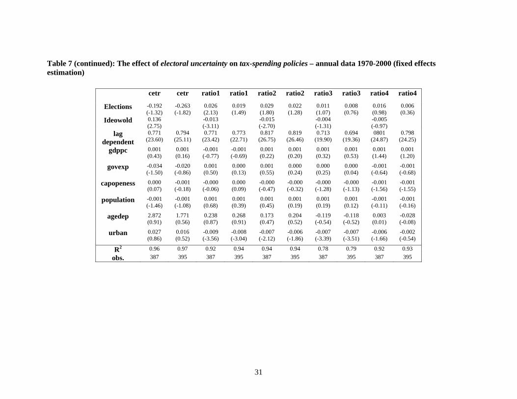
31

Table 7 (continued): The effect of electoral uncertainty on tax-spending policies – annual data 1970-2000 (fixed effects estimation)

cetr cetr ratio1 ratio1 ratio2 ratio2 ratio3 ratio3 ratio4 ratio4

Elections -0.192 (-1.32)

-0.263 (-1.82)

0.026 (2.13)

0.019 (1.49)

0.029 (1.80)

0.022 (1.28)

0.011 (1.07)

0.008 (0.76)

0.016 (0.98)

0.006 (0.36)

Ideowold 0.136 (2.75)

-0.013 (-3.11)

-0.015 (-2.70)

-0.004 (-1.31)

-0.005 (-0.97)

lag dependent

0.771 (23.60)

0.794 (25.11)

0.771 (23.42)

0.773 (22.71)

0.817 (26.75)

0.819 (26.46)

0.713 (19.90)

0.694 (19.36)

0801 (24.87)

0.798 (24.25)

gdppc

0.001 (0.43)

0.001 (0.16)

-0.001 (-0.77)

-0.001 (-0.69)

0.001 (0.22)

0.001 (0.20)

0.001 (0.32)

0.001 (0.53)

0.001 (1.44)

0.001 (1.20)

govexp

-0.034 (-1.50)

-0.020 (-0.86)

0.001 (0.50)

0.000 (0.13)

0.001 (0.55)

0.000 (0.24)

0.000 (0.25)

0.000 (0.04)

-0.001 (-0.64)

-0.001 (-0.68)

capopeness

0.000 (0.07)

-0.001 (-0.18)

-0.000 (-0.06)

0.000 (0.09)

-0.000 (-0.47)

-0.000 (-0.32)

-0.000 (-1.28)

-0.000 (-1.13)

-0.001 (-1.56)

-0.001 (-1.55)

population

-0.001 (-1.46)

-0.001 (-1.08)

0.001 (0.68)

0.001 (0.39)

0.001 (0.45)

0.001 (0.19)

0.001 (0.19)

0.001 (0.12)

-0.001 (-0.11)

-0.001 (-0.16)

agedep

2.872 (0.91)

1.771 (0.56)

0.238 (0.87)

0.268 (0.91)

0.173 (0.47)

0.204 (0.52)

-0.119 (-0.54)

-0.118 (-0.52)

0.003 (0.01)

-0.028 (-0.08)

urban

0.027 (0.86)

0.016 (0.52)

-0.009 (-3.56)

-0.008 (-3.04)

-0.007 (-2.12)

-0.006 (-1.86)

-0.007 (-3.39)

-0.007 (-3.51)

-0.006 (-1.66)

-0.002 (-0.54)

R2 0.96 0.97 0.92 0.94 0.94 0.94 0.78 0.79 0.92 0.93 obs. 387 395 387 395 387 395 387 395 387 395

do political incentives matter for tax policies? ideology, opportunism

Documents